master thesis selection in a heap - aarhus universitet · 1.initialize priority queue pq with all...
TRANSCRIPT

Master Thesis
Selection in a Heap
Kenn Daniel20118457
kenn [email protected]
Casper Færgemand20118354
Advisor: Gerth Stølting Brodal
June 13, 2016
1

Abstract
We test the algorithms presented by Frederickson [5] and investigate if theyfollow the theoretical bounds, with a focus on whether the theoretical lineartime algorithm can be used in practice. We do this by implementing thealgorithms (link in Table 0.1), and then measuring and comparing them onseveral parameters. Additionally we also reproduce the theoretical results to ahigher degree of detail.
In Danish
Vi tester algoritmerne præsenteret af Frederickson [5] og undersøger om de følgerde teoretiske grænser, med fokus pa om algoritmen med teoretisk lineærtidskompleksitet kan bruges i praksis. Dette gjorde vi ved at implementerealgoritmerne (link i Table 0.1), og derefter male og sammenlige dem pa adskilligeparametre. Derudover efterprøver vi de teoretiske resultater med en højeregrad af detalje.
github.com/HeapSelection/Heap-Selection
Table 0.1: Link to implementations
2

Contents
Contents 3
1 Introduction 6
2 Notation 8
3 Naive Algorithm O(k · log k) 10
3.1 Introduction . . . . . . . . . . . . . . . . . . . . . . . . . . . . . 10
3.2 The algorithm . . . . . . . . . . . . . . . . . . . . . . . . . . . . 10
3.3 Termination . . . . . . . . . . . . . . . . . . . . . . . . . . . . . 11
3.4 Correctness . . . . . . . . . . . . . . . . . . . . . . . . . . . . . 11
3.5 Theoretical bound . . . . . . . . . . . . . . . . . . . . . . . . . 11
4 Framework 12
4.1 Introduction . . . . . . . . . . . . . . . . . . . . . . . . . . . . . 12
4.2 Partitioning . . . . . . . . . . . . . . . . . . . . . . . . . . . . . 12
4.3 Clans . . . . . . . . . . . . . . . . . . . . . . . . . . . . . . . . 12
4.4 Recursion . . . . . . . . . . . . . . . . . . . . . . . . . . . . . . 13
4.5 Priority queue preservation . . . . . . . . . . . . . . . . . . . . 14
4.6 Category . . . . . . . . . . . . . . . . . . . . . . . . . . . . . . . 14
5 Select 16
5.1 Introduction . . . . . . . . . . . . . . . . . . . . . . . . . . . . . 16
5.2 The algorithm . . . . . . . . . . . . . . . . . . . . . . . . . . . . 16
5.3 Further reading . . . . . . . . . . . . . . . . . . . . . . . . . . . 18
6 Clans 19
6.1 Clan . . . . . . . . . . . . . . . . . . . . . . . . . . . . . . . . . 19
6.2 Clan-3 . . . . . . . . . . . . . . . . . . . . . . . . . . . . . . . . 20
6.3 Clan-4 . . . . . . . . . . . . . . . . . . . . . . . . . . . . . . . . 20
7 SEL1 O(k · log log k) 21
7.1 Introduction . . . . . . . . . . . . . . . . . . . . . . . . . . . . . 21
7.2 The algorithm . . . . . . . . . . . . . . . . . . . . . . . . . . . . 21
3

4 CONTENTS
7.3 Termination . . . . . . . . . . . . . . . . . . . . . . . . . . . . . 227.4 Correctness . . . . . . . . . . . . . . . . . . . . . . . . . . . . . 227.5 Theoretical bound . . . . . . . . . . . . . . . . . . . . . . . . . 22
8 SEL2 O(k · 3log∗(k)) 248.1 Introduction . . . . . . . . . . . . . . . . . . . . . . . . . . . . . 248.2 The algorithm . . . . . . . . . . . . . . . . . . . . . . . . . . . . 248.3 Termination . . . . . . . . . . . . . . . . . . . . . . . . . . . . . 258.4 Correctness . . . . . . . . . . . . . . . . . . . . . . . . . . . . . 258.5 Theoretical bound . . . . . . . . . . . . . . . . . . . . . . . . . 26
9 Priority queues 309.1 Introduction . . . . . . . . . . . . . . . . . . . . . . . . . . . . . 309.2 The data structure . . . . . . . . . . . . . . . . . . . . . . . . . 309.3 Termination . . . . . . . . . . . . . . . . . . . . . . . . . . . . . 319.4 Correctness . . . . . . . . . . . . . . . . . . . . . . . . . . . . . 319.5 Theoretical bounds . . . . . . . . . . . . . . . . . . . . . . . . . 329.6 Consequences of splitting . . . . . . . . . . . . . . . . . . . . . 33
10 SEL3 O(k · 2log∗(k)) 3410.1 Introduction . . . . . . . . . . . . . . . . . . . . . . . . . . . . . 3410.2 The algorithm . . . . . . . . . . . . . . . . . . . . . . . . . . . . 3410.3 Termination . . . . . . . . . . . . . . . . . . . . . . . . . . . . . 3510.4 Correctness . . . . . . . . . . . . . . . . . . . . . . . . . . . . . 3610.5 Theoretical bound . . . . . . . . . . . . . . . . . . . . . . . . . 36
11 SEL4 O(k) 4111.1 Introduction . . . . . . . . . . . . . . . . . . . . . . . . . . . . . 4111.2 The algorithm . . . . . . . . . . . . . . . . . . . . . . . . . . . . 4111.3 Termination . . . . . . . . . . . . . . . . . . . . . . . . . . . . . 4311.4 Correctness . . . . . . . . . . . . . . . . . . . . . . . . . . . . . 4311.5 Theoretical bound . . . . . . . . . . . . . . . . . . . . . . . . . 45
12 Examples 5212.1 Naive . . . . . . . . . . . . . . . . . . . . . . . . . . . . . . . . 5212.2 SEL1 and SEL2 . . . . . . . . . . . . . . . . . . . . . . . . . . . 5412.3 SEL3 and SEL4 . . . . . . . . . . . . . . . . . . . . . . . . . . . 57
13 SEL4 parameter optimization 6513.1 Introduction . . . . . . . . . . . . . . . . . . . . . . . . . . . . . 6513.2 Choice of Parameters . . . . . . . . . . . . . . . . . . . . . . . . 65
14 Experiment heaps 6814.1 Worst case . . . . . . . . . . . . . . . . . . . . . . . . . . . . . . 6814.2 Random case . . . . . . . . . . . . . . . . . . . . . . . . . . . . 68

CONTENTS 5
14.3 Best case . . . . . . . . . . . . . . . . . . . . . . . . . . . . . . 69
15 Priority Queue Trouble 71
16 Experimental results 7416.1 System specification . . . . . . . . . . . . . . . . . . . . . . . . 7416.2 Runtime . . . . . . . . . . . . . . . . . . . . . . . . . . . . . . . 7416.3 Comparisons . . . . . . . . . . . . . . . . . . . . . . . . . . . . 8116.4 Accesses . . . . . . . . . . . . . . . . . . . . . . . . . . . . . . . 8516.5 Conclusion . . . . . . . . . . . . . . . . . . . . . . . . . . . . . 89
17 Valgrind Results 9117.1 Worst case . . . . . . . . . . . . . . . . . . . . . . . . . . . . . . 9217.2 Random case . . . . . . . . . . . . . . . . . . . . . . . . . . . . 9717.3 Best case . . . . . . . . . . . . . . . . . . . . . . . . . . . . . . 10317.4 Conclusion . . . . . . . . . . . . . . . . . . . . . . . . . . . . . 109
18 Conclusion 111
19 Theorems 112
Bibliography 114

Chapter 1
Introduction
Given a binary min-heap of size n � k, we want to select the k smallestelements. Since n� k we will view this binary min-heap as being infinitelylarge. Here a binary min-heap is a heap ordered binary tree, where every nodecontains a value, and has two children. The children of a node have valueshigher than or equal to that of their parent. The min-heap was introduced byWilliams [6]. An example of our problem is seen in Figure 1.1, where we haveselected the five smallest elements.
Frederickson [5] describes four algorithms with increasingly better upperbounds, with the final algorithm SEL4 having the optimal theoretical bound of
Figure 1.1: An infinitely large heap with the 5 smallest elements colored.
6

7
O(k). In this thesis we have investigated the practicalities of these algorithmsand assessed whether or not, especially the final optimal bound, works inpractice. This we have done by implementing all the algorithms mentioned,and then measure their behaviours on different parameters such as, but notlimited to: comparisons, accesses to the original heap and last level data cachemisses.
Furthermore, because of how advanced some of the algorithms describedby Frederickson in [5] are, another issue can be the understanding of them.Frederickson does provide some intuition by constructing the next algorithmthrough the addition of one or more paradigms to the previous. Thus buildingthe algorithms iteratively. Despite Frederickson’s efforts, understanding ofthe algorithms is not achieved without difficulty. We therefore try to giveadditional explanations, intuition and show how the algorithms work throughexamples.
Throughout this thesis we have also proven several unproven claims pro-posed by Frederickson [5], some claims we have not managed to prove, but forthese we have tried to give some intuition into why they could hold.
Selection in a min-heap has 62 citations at the time of writing. Eppstein[4] uses it in an algorithm that finds the k shortest paths. Brodal [2] uses it inan algorithm that selects the k largest sums of subarrays in an array.

Chapter 2
Notation
Table 2.1: Table of Notation
T Our original infinitely large min-heap.H0 The root of T .k The number of small elements we are selecting.r Natural number, we use for representing subroutine sizes.B Clan size.C A clan.Ci Clan number i.
os(C) The off-spring of clan C.pr(C) The poor-relation of clan C.H A set of nodes from our infinite min-heap.
PQ A priority queue.
8

9
Table 2.2: Table of Function Definitions
na = aa··a︸︷︷︸
n
log∗(r) =
{1 if r ≤ 2
1 + log∗(dlog(r)e) otherwise
f(r) =
⌊(dlog(r)elog∗(r)
)2⌋
h3(r) =
{1 if r ≤ 1
h3(blog(r)c) ·⌈
rh3(blog(r)c)
⌉otherwise
h4(r) =
{1 if r ≤ 1
h4(f(r)) ·⌈
rh4(f(r))
⌉otherwise
A(r) =
2·log∗(r)∏i=1
(1 +4
i2)
B(r) =r
3log∗(r) · (r ·A(r)−
⌈r
blog(r)c
⌉· blog(r)c ·A(blog(r)c))
C(r) =(log∗(r))2((2 log∗(r)− 1)2 + 4)
4dlog∗(r)e2 log∗(r)∏
i=1(1 + 4
i2)

Chapter 3
Naive Algorithm O(k · log k)
3.1 Introduction
The first and simplest algorithm for selecting the k smallest elements in a minheap uses a minimum priority queue holding heap nodes. It takes an integer kand a heap node H0 as arguments and returns the k smallest elements foundin the tree rooted in H0. It is only briefly described in Frederickson’s paper[5], but it is fairly easy to come up with. An example of how it works can beseen in Chapter 12. In algorithm SEL1, which improve the bound O(k · log k)to O(k · log log k) and will be presented later, the Naive algorithm is used andis required to find the k smallest elements from a list of trees, represented bytheir roots. The single tree version simply calls the multiple tree version. Inthe multiple tree version we call the set of trees Hn. It works as follows:
1. Initialize priority queue PQ with all elements from Hn
2. Initialize result list R
3. k times do:
a) Ei := extractMin(PQ)
b) Add Ei to R
c) Insert left and right child of Ei into PQ
4. Return R
3.2 The algorithm
We begin by initializing a priority queue PQ, where smaller elements havehigher priority, and add the elements in Hn to PQ. Hn will only contain oneelement, namely H0 when called as the single tree version, but will maximallyhold O(k) elements when called through SEL1. Then we perform extractMin
10

3.3. TERMINATION 11
operations on PQ k times, and for each of these times we store the elementwe extracted as a part of the result. For every node extracted we then insertits children into the PQ. When k elements have been extracted we are done.
3.3 Termination
In order to argue that the algorithm terminates we first note that we makethe assumption that we pick a priority queue for which the operations allterminate, given that the priority queue has a finite size. With this establishedour algorithm clearly terminates since we specifically call the extract-minoperation k times. Since we only ever extract k elements, and every elementhas at most two children, the size of the priority queue will never exceed O(k)elements, which means the size of the priority queue is indeed finite.
More precisely, if Hn holds s elements, then the maximum size of thepriority queue will be s + k, because we k times extract one element and addtwo, effectively raising the queue size by one. Since s = O(k), we have thatthe maximum priority queue size is O(k).
3.4 Correctness
To achieve correctness the important invariant is that everything that will beinserted into our priority queue in the future has an ancestor in the priorityqueue, and every element extracted is smaller than all the elements we havenot extracted. Since we start with root(s) of trees, it is easy to see that sincewe always insert both children of an extracted element we will not miss anynodes in the trees we are looking for minimum elements in. Additionally sincewe are working on a minimum priority queue it is clear that when we extractan element this element is the smallest in the priority queue at the time ofextraction. Since we are selecting the smallest elements from a minimum heap,and we add the children of any extracted element, every time we extract anelement this element will be the minimum element that was left. Which is whywhen he have extracted k elements we will have extracted the k smallest.
3.5 Theoretical bound
By the argument in Section 3.3 the priority queue will have size O(k). Thismeans the extractMin operation will achieve a bound of O(log(k)) for a suitablechoice of data structure to represent the priority queue (a minimum heap).Since we call extractMin k times we achieve a total bound of O(k · log(k)).

Chapter 4
Framework
4.1 Introduction
The four algorithms for finding the k smallest elements a min heap presentedby Frederickson in [5] gradually improve upon the naive algorithm presented inChapter 3. The paper presents multiple ideas that when used together providethe algorithm SEL4, which has an optimal linear theoretical bound.
These ideas also provide entry points for tweaking a practical implementa-tion of several of the algorithms. In this chapter the ideas will be presented inthe order they appear in [5], and some will be supplemented with a discussionof how the runtime is affected by changing parameters in the implementation.
4.2 Partitioning
Instead of directly finding the elements requested, we search for an element xwith a rank that is greater than or equal to the rank of k’th smallest element.We then traverse the heap, adding all elements less than or equal to x to a list.This can result in more than k elements. To fix this the list can be partitionedusing a standard partition algorithm, so that the k smallest elements are atthe beginning of the list and the rest of the elements in the list are discarded.
See Chapter 5 for details. All four algorithms described by Frederickson in[5] use this technique, see Chapters 7, 8, 10, and 11.
4.3 Clans
An element of appropriate rank can be used to find the k smallest elements,see above section. This gives some freedom as to how elements are handled.
The four algorithms, SEL1, SEL2, SEL4, and SEL4, still use priority queuesinternally to keep track of which elements have been found. To reduce thetime used by the priority queue we group elements into clans, and instead putthe clans into the priority queues. For instance, if we let a clan contain
√k
12

4.4. RECURSION 13
elements, we can reduce the number of extractMin and insert operations by afactor
√k and still obtain k elements.
The value of a clan is called a representative, which is used in the priorityqueue for ordering, and it is the largest member of the clan. Thus if thealgorithm runs extractMin k
clansize times, a total of k elements will have beenextracted through the clans. Since the clans are ordered by representative andthe lowest ranked clans are extracted first, the representative of the last clanmust be larger than or equal to all other elements in extracted clans, and thushave a rank of at least k.
When a clan is extracted from the priority queue, we create new clans.The way this is done is relevant to the time bounds, but not to correctness. Inregard to time bounds, if a clan is to be made with elements from a very largeset of elements it follows that the smallest elements cannot be found fast: Ifwe are to find the k smallest among 2k unordered elements, we cannot hope todo so in O(k) time. Therefore the four algorithms supply ways to split the setsof possible clan members into smaller sets. The method presented by SEL1and SEL2 is considerably more complicated than the one presented by SEL3and SEL4, but they both achieve the exact same thing: Splitting the set intoa smaller size.
See Chapter 6 for details on clans and Chapters 7, 8, 10, and 11 for theiruse.
Tweaking
Clan size is relevant to time bounds, but not to correctness (within reasonablelimits). If the clan size is set to 1, the algorithm essentially degenerates tothe naive algorithm, with some overhead. Conversely, if the clan size is setto k, meaning we only need a single clan to get an element of at least rankk, we simply push the entire problem to whatever subroutine we’re calling.For SEL1, this means simply asking the naive algorithm to solve the entireproblem. For the recursive algorithms, continuously requesting clans of size kobviously breaks the termination proof (see reasonable limits above).
4.4 Recursion
We have changed the problem of finding the k smallest elements in H0 tofinding the r smallest in some subset of H0 multiple times. If the time boundscan be improved by solving subproblems in the main algorithm, and theproblem solved by the subroutine is very similar to the main problem, the nextlogical step is to apply our subroutine recursively: If the top layer is askedfor k elements and it runs the subroutine asking for f(k) elements for somedefinition of f , the next layer can call itself asking for f(f(k)) elements. Werefer to the rank of the element requested at any level as r, with r = k at thetop level, and r = 1 as the base case for the recursion.

14 CHAPTER 4. FRAMEWORK
See SEL2, SEL3, and SEL4 in Chapters 8, 10, and 11 respectively for usageof recursion.
Tweaking
The recursion depth is an obvious place to tweak the algorithms. Essentially, thenaive algorithm, SEL1, and SEL2 behave the same way. The naive algorithmhas a recursion depth of 0, solving all of its work up front. SEL1 has a recursiondepth of 1, cutting its work up once and then letting the naive algorithm solveit. SEL2 recurses until it reaches its base case of r = 1. Changing the basecase to something larger than 1 could be a way to improve SEL2.
Unfortunately, in the case of SEL1 and SEL2, neither perform better thanthe naive algorithm in our runtime tests, so having a recursion depth of 0 isbest. With a lot of extrapolation, SEL1 could possibly beat the naive algorithmif used on more data than we were able to generate. See Chapter 16 for details.
SEL4 has a chapter dedicated to tweaking the base case and will not bediscussed here. See Chapter 13. SEL3 might benefit from some of the sameoptimizations, but since SEL4 is better than SEL3 in all measurements, it hasnot been examined.
4.5 Priority queue preservation
In the introduced recursion, elements are considered multiple times. Forinstance, if we are at layer ` and extract a clan from our priority queue, thatclan was created at layer ` + 1. When we return a clan from our level, wethrow away our priority queue, and thus work done at this and lower levelswill have to be redone if needed at a later time: The same elements that werealready found previously might be found in subsequent calls.
The idea is then to try to reuse information from lower levels of the recursion.We want a guarantee that any element is extracted at most once per level.
This is done by adding the priority queue used at level ` + 1 to the clanreturned to level `. When level ` later calls the subroutine for ` + 1, it passesalong the priority queue. This means work already done is essentially preservedbetween calls to the same level. An important property is that we need tosplit a priority queue in sublinear time to stay within time bounds.
See Chapter 9 for details on priority queue splitting.
4.6 Category
When we extract a clan from a priority queue, we create two new clans (seeChapters 6, and 9). In a rather obscure way of improving the time bounds, thelast algorithm, SEL4, presents the idea of sometimes not splitting. It worksas follows: When a clan C is first inserted into the priority queue, give it a

4.6. CATEGORY 15
category of 1. When C is extracted, if the category is below some threshold(based on r in SEL4), do not split its priority queue, but simply recurse on it.The resulting clan C ′ is given the category cat(C) + 1 and then inserted intoour priority queue. If cat(C) > threshold, we split and recurse on both. Theresulting clans are both given a category of 1. Since the threshold for splittingis proportional to r, deeper in the recursion we split more often.
Tweaking
Splitting threshold is relevant to time bounds, but not to correctness: Settingthe threshold to 1, meaning we always split, we are no different from SEL3.The other extreme of never splitting also loses the time bound, but is also stillcorrect: Never splitting means all layers of recursion will only ever have oneclan in their priority queues, except the the layer where r = 1, where we getO(k) clans, essentially the naive algorithm.
In our tests we found that changing the threshold had some effect, butchanging the base case had a much greater effect, see Chapter 13.

Chapter 5
Select
5.1 Introduction
The four algorithms presented by Frederickson in [5] all use a selection algorithmfor finding the k smallest elements in a list.
Blum presents an algorithm called PICK in [1], which finds the i’th smallestnumber in a list. In Chapter 9.3 in Corman [3], SELECT is described. SELECTbuilds on PICK and additionally partitions the list such that all elementsbefore the k’th are less than or equal, and all later elements are greater thanor equal. Select presented here is a variation of SELECT.
5.2 The algorithm
Select takes arguments k and A, k being the number of elements desired, Abeing the list of elements. It then looks at A in its entirety and calls thesubroutine findMedian on A. It partitions A around the median. If the medianis at a position different to k, repeat on a subset of A. The partitioning isdone in place. It looks as follows:
1. low := 0
2. high := length(A)
3. While (low < high) do:
a) index := low
b) findMedian(A, low, high)
c) swap(A[low], A[high− 1])
d) i := low − 1
e) j := low
f) While (j < high− 1) do:
16

5.2. THE ALGORITHM 17
i. If (value(A[j]) ≤ value(A[high− 1]):
A. i := i + 1
B. swap(A[i], A[j])
ii. j := j + 1
g) swap(A[i + 1), A[high− 1]
h) index := i + 1
i) If (index < k):
i. low := index + 1
j) Else if (k < index):
i. high := index
k) Else:
i. Return
The findMedian subroutine takes A, a list of elements, and low and high, therange in which a median is to be found. It works by finding exact medians offixed sized subsets of A, and combining these medians to create approximatemedians of large parts of A, until eventually it condenses to a single value.This final value is not the exact median, but a good approximation, see [3].
In the following example the fixed size for exact medians is 9. The medianit finds will be swapped to the beginning on the part of A it operates on. Itlooks as follows:
1. remaining := high− low
2. While (remaining > 0) do:
a) index := low
b) extra := remaining%9
c) i := 0
d) While (i < remaining)
i. If (i + 9 < remainder):
A. sort(A[i + low], A[i + low + 9])
B. swap(A[index], A[low + i + 4])
ii. Else:
A. sort(A[i + low], A[low + remaining])
B. swap(A[index], A[low + i + extra−12 ])
iii. i := i + 9
iv. index := index + 1
e) remaining := remaining9

18 CHAPTER 5. SELECT
f) If (extra 6= 0):
i. remaining := remaining + 1
Note that our pseudo code finds the median of 9 elements, which is what theimplementation uses. The algorithm described by Cormen in [3] finds themedian of 5 elements, but is otherwise the same.
5.3 Further reading
The details of Select are not relevant to SEL1, SEL2, SEL3, and SEL4, andwill not be discussed. The particular Select used in the implementation couldbe replaced by any other Select, so long as it runs in linear time. For a detailedoverview of Select, see Chapter 9.3 in Cormen [3].

Chapter 6
Clans
6.1 Clan
For the algorithm in the next chapters we will use something Frederickson [5]calls clans. A clan C contains some amount of nodes from the original heap T ,a representative of the clan rep(C), a set of nodes called the off-spring os(C),and a set of nodes called the poor-relation pr(C).
When we construct a clan C, we construct it from some forest A. Herethe off-spring is then defined as the children of the nodes in C which are notthemselves in C. The poor-relation is defined as the set of nodes in A, whichare not in C. Lastly the representative of the clan C is defined as the largestvalue of any node in C.
The members of C are found from the roots in A, with each algorithmspecifying its own way of doing so.
Off-spring and poor-relation are found in the following way, with thefunction createClan taking C and A:
1. All nodes in C and A start uncolored. Color all nodes in C.
2. For each node in children of nodes in C, if the node is uncolored, add itto os(C).
3. For each node in A, if the node is uncolored, add it to pr(C).
4. Remove color from nodes in C.
This ensures all nodes are uncolored when the algorithm terminates. Becauseall nodes in C are colored first, nodes in C cannot appear in os(C) or pr(C).
The construction of a clan given A and C is linear in the size of A andC, since the four sets are each iterated a constant number of times. This isasymptotically optimal.
19
20 CHAPTER 6. CLANS
6.2 Clan-3
Clan-3, used by SEL3, is a simpler construct than the previously defined clan.Clan-3 contains a representative and a heap as defined in chapter 9. Themembers of the clan are implicit in that they are smaller than or equal to therepresentative, and not included in the heap. The heap is a substitute for thepreviously used off-spring and poor-relation: the heap itself can be split intotwo, removing the need for a distinction between the different kinds of nodesnot included in the clan.
6.3 Clan-4
Clan-4, used by SEL4, is identical to clan-3 defined above, except that itcontains an additional integer value called category, which SEL4 uses.

Chapter 7
SEL1 O(k · log log k)
7.1 Introduction
For our second algorithm we have implemented the first described algorithmby Frederickson [5]. We have illustrated how this algorithm works in Chapter12.
7.2 The algorithm
SEL1 is an algorithm that uses clans of blog(k)c size to find an element withrank between k and 2k. The problem of finding the clans in subtrees fromH0 is solved by the naive algorithm. SEL1 takes two arguments, an integer kand H0, then calls Select (See Chapter 5) on the last representative found. Itworks as follows:
1. clanSize := blog(k)c
2. C0 := createClan(naive(clanSize,H0))
3. Initialize heap PQ with C0
4. highest := − inf
5. limit :=⌈
kclanSize
⌉6. limit times do:
a) Ci := extractMin(PQ)
b) highest := rep(Ci)
c) If size(os(Ci)) > 0:
i. Insert createClan(naive(clanSize, os(Ci))) into PQ
d) If size(pr(Ci)) > 0:
21

22 CHAPTER 7. SEL1 O(k · log log k)
i. Insert createClan(naive(clanSize, pr(Ci))) into PQ
7. Do a breadth first search and Select (See 5) using highest according tochapter 5
7.3 Termination
This algorithm clearly terminates since we have already established that theNaive algorithm terminates, and we only do a fixed number of iterations. Likefor the Naive algorithm the size of the priority queue PQ is finite, becausewe first add one clan made from the element the algorithm is called with.Then we limit times call extract and two clans made from the off-spring andpoor-relation of the extracted clan. This means we limit times at most growthe size of the priority queue by one.
7.4 Correctness
For proof of correctness we first note that every clan is disjoint. Additionally
since we extract⌈
kblog(k)c
⌉clans from our priority queue, we have that the
representative for the last extracted clan is larger than the values for all nodes
in all our previously extracted clans, and since we have extracted⌈
kblog(k)c
⌉clans of size blog(k)c we have that this last representative must be at least aslarge as the kth smallest element, and also it must be no larger than the 2 · kthsmallest element, because for every clan we extract we make at most two new
clans. Since we extract⌈
kblog(k)c
⌉clans we make at most:
2 · (⌈
k
blog(k)c
⌉) ≤ 2 · ( k
blog(k)c+ 1) (7.1)
clans, and since every clan has size blog(k)c, we have at most:
2 · ( k
blog(k)c+ 1) · blog(k)c = 2 · k + 2 · blog(k)c (7.2)
elements in all of these clans in total. Since our last extracted clan has arepresentative larger than or equal to all other elements in previously extractedclans we have that there can be at most 2 · k of these elements less than orequal to our last representative. We remove the 2 · blog(k)c term because theseare the elements created by our last extracted clan.
7.5 Theoretical bound
The bottleneck in our algorithm is the part where we call our Naive algorithm
for every one of our⌈
kblog(k)c
⌉iterations. Since our Naive algorithm runs in

7.5. THEORETICAL BOUND 23
c′ · r · log(r), where r is the number of smallest elements we want to find andc′ is some constant, we get in total. We will assume that k > 1, since for k = 1the problem is easy, we get:
c′ · blog(k)c · log(blog(k)c) ·⌈
k
blog(k)c
⌉≤ c′ · blog(k)c · log(blog(k)c) · ( k
blog(k)c+ 1)
≤ c′ · log(blog(k)c) · k + c′ · log(blog(k)c) · blog(k)c≤ 2c′ · log(blog(k)c) · k≤ 2c′ · log(log(k)) · k= O(k · log(log(k)))
which is our asymptotic bound. Furthermore we need to show that we do notuse too long in our last step of the algorithm where we call a k-select algorithmon lists. Referring to Chapter 5 we can see that this step will only take O(k)time on a list of size maximum 2 · k. We get the asymptotic bound we werelooking for.

Chapter 8
SEL2 O(k · 3log∗(k))
8.1 Introduction
We have implemented the second algorithm described by Frederickson [5] calledSEL2. We have illustrated how this algorithm works in Chapter 12.
8.2 The algorithm
SEL2 is a recursive algorithm that uses clans of blog(k)c size to find an elementwith rank between k and 2k. In SEL1 the problem of finding the members ofeach clan was solved using the naive algorithm, while here we use SEL2 itself.SEL2 takes two arguments, r and H.
Note that Frederickson [5] also mentions RSEL2, but since that and SEL2do virtually the same, RSEL2 was ignored.
We’ve changed the name of k to r, as it also refers to the elements neededto solve sub problems. It works as follows:
1. If r = 1, return the smallest element in H.
2. Partition H into subsets H1,H2, . . . ,Hs with |Hi| ≤ 2blog(r)c.
3. Let Ci := createClan(SEL2(Hi, blog(r)c),Hi).
4. Initialize heap PQ with every Ci.
5. Let limit :=⌈
rblog(r)c
⌉.
6. limit times do:
a) Let Cj := PQ.extractMin().
b) Let Ci := createClan(RSEL2(os(Cj), blog(r)c), Cj).
c) Let Ci+1 := createClan(RSEL2(pr(Cj), blog(r)c), Cj).
24

8.3. TERMINATION 25
d) PQ.insert(Ci).
e) PQ.insert(Ci+1).
7. Let Cj be the last extracted element from step 6.a.
8. Add the elements in H less than or equal to rep(Cj) to list L.
9. Select the r smallest elements in L and return them.
8.3 Termination
The recursive call in 3, 6.b, and 6.c each happen a bounded number of times,and each recursive call has a smaller r with a base case of r = 1, so thealgorithm terminates. Additionally by argumentation very similar to that ofthe Naive algorithm and SEL1, the priority queue is finite in size.
8.4 Correctness
The proof of correctness is an induction proof and we note that every clan isdisjoint.
The base case is r = 1 in which the algorithm returns the smallest node inH. This is trivially correct.
For the induction case we assume that the algorithm works for r′ < r,which means that all the recursive calls are correct. The steps 7, 8, 9 requirethe rank of r ≤ rep(Cj), so the algorithm is correct if this is true.
Each clan extracted from PQ has size blog(r)c and in total⌈
rblog(r)c
⌉clans
are extracted. That means a minimum of
blog(r)c ·⌈
r
blog(r)c
⌉≥ blog(r)c · r
blog(r)c= r
nodes have been extracted, and the representative of the last clan extracted isgreater than or equal to the nodes found in all the extracted clans. Thus thelast representative has a rank of at least r.
The above requires that no clans have nodes in common. To prove that thisis the case, we note that the clans give two sets of nodes from which new clanscan be made, namely off-spring and poor-relation. Off-spring specifically doesnot include nodes also included in the clan it belongs to, and poor-relationis nodes in H not included in the clan. Neither off-spring nor poor-relationcontain nodes that are ancestors of each other. This means that once a clan iscreated, its nodes will never be included in another clan.
26 CHAPTER 8. SEL2 O(k · 3log∗(k))
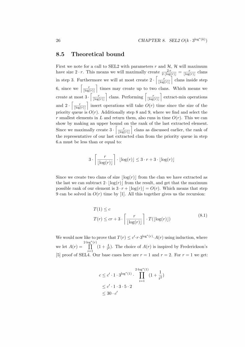
8.5 Theoretical bound
First we note for a call to SEL2 with parameters r and H, H will maximumhave size 2 · r. This means we will maximally create 2·r
2·blog(r)c = rblog(r)c clans
in step 3. Furthermore we will at most create 2 ·⌈
rblog(r)c
⌉clans inside step
6, since we⌈
rblog(r)c
⌉times may create up to two clans. Which means we
create at most 3 ·⌈
rblog(r)c
⌉clans. Performing
⌈r
blog(r)c
⌉extract-min operations
and 2 ·⌈
rblog(r)c
⌉insert operations will take O(r) time since the size of the
priority queue is O(r). Additionally step 8 and 9, where we find and select ther smallest elements in L and return them, also runs in time O(r). This we canshow by making an upper bound on the rank of the last extracted element.
Since we maximally create 3 ·⌈
rblog(r)c
⌉clans as discussed earlier, the rank of
the representative of our last extracted clan from the priority queue in step6.a must be less than or equal to:
3 ·⌈
r
blog(r)c
⌉· blog(r)c ≤ 3 · r + 3 · blog(r)c
Since we create two clans of size blog(r)c from the clan we have extracted asthe last we can subtract 2 · blog(r)c from the result, and get that the maximumpossible rank of our element is 3 · r + blog(r)c = O(r). Which means that step9 can be solved in O(r) time by [1]. All this together gives us the recursion:
T (1) ≤ c
T (r) ≤ cr + 3 ·⌈
r
blog(r)c
⌉· T (blog(r)c)
(8.1)
We would now like to prove that T (r) ≤ c′·r·3log∗(r)·A(r) using induction, where
we let A(r) =2·log∗(r)∏
i=1(1 + 4
i2). The choice of A(r) is inspired by Frederickson’s
[5] proof of SEL4. Our base cases here are r = 1 and r = 2. For r = 1 we get:
c ≤ c′ · 1 · 3log∗(1) ·
2·log∗(1)∏i=1
(1 +1
i2)
≤ c′ · 1 · 3 · 5 · 2≤ 30 · c′

8.5. THEORETICAL BOUND 27
So for the base case r = 1 we should set c′ ≥ 130 · c. Now for r = 2. We start
out by calculating the left side:
T (2) ≤ 2c + 3 ·⌈
2
blog(2)c
⌉· T (blog(2)c)
≤ 2c + 3 ·⌈
2
1
⌉· c
= 8c
Now for the right side:
c′ · 2 · 3log∗(2) ·
2·log∗(2)∏i=1
(1 +4
i2)
= c′ · 2 · 3 · 10
= 60c′
Which means we need 8c ≤ 60c′, which gives us that we should set 860c = 2
15c ≤c′ for the second base case to hold. Now that we have the two base cases wewant to show the case r > 2 using induction. For the inductive case assumethe claim is true for r′ < r. We will here use A(r), rather than substituting itwith what it equals. We show:
T (r) ≤ cr + 3
⌈r
blog(r)c
⌉· T (blog(r)c) (Eq. 8.1)
≤ cr + 3
⌈r
blog(r)c
⌉· c′blog(r)c3log
∗(blog(r)c) ·A(blog(r)c) (Ind. hypo.)
≤ cr +
⌈r
blog(r)c
⌉· c′blog(r)c3log
∗(blog(r)c)+1 ·A(blog(r)c)
≤ cr +
⌈r
blog(r)c
⌉· c′blog(r)c3log
∗(r) ·A(blog(r)c) (Def. log∗)
We then need:
cr +
⌈r
blog(r)c
⌉· c′blog(r)c3log
∗(r) ·A(blog(r)c) ≤ c′ · r · 3log∗(r) ·A(r)
Moving around we get:
cr ≤ c′ · 3log∗(r) · (r ·A(r)−
⌈r
blog(r)c
⌉· blog(r)c ·A(blog(r)c))
Isolating c′ we obtain:
r
3log∗(r) · (r ·A(r)−
⌈r
blog(r)c
⌉· blog(r)c ·A(blog(r)c))
· c ≤ c′

28 CHAPTER 8. SEL2 O(k · 3log∗(k))
Figure 8.1: B(r) over r. With r ∈ [3, 200].
If the expression r
3log∗(r)·(r·A(r)−
⌈r
blog(r)c
⌉·blog(r)c)
converges we can pick c′ such
that our proof by induction holds. Which would mean we have shown thatT (r) is O(r · 3log∗(r) ·A(r)), which for the A(r) we have chosen is O(r · 3log∗(r)),because our choice of A(r) converges, which can be seen using Theorem 19.0.1and Theorem 19.0.2. If we call our long expression for B(r) we get:
B(r) =r
3log∗(r) · (r ·A(r)−
⌈r
blog(r)c
⌉· blog(r)c ·A(blog(r)c))
And what remains is to show that this expression converges. We have tried forlong to show this, but have been unable to. We should note that Fredericksonrefrains from showing this in [5], and just states that the recursion is boundedby O(r ·3log∗(r)) on page 204. Looking at Figure 8.1 and Figure 8.2 there seemsto be an indication that B(r) does converge, and it looks like the value neverexceeds 0.025 = 1
40 . So if it does converge as indicated by the two figures, wecould set 1
40 · c ≤ c′.Lastly as argued earlier the representative of the last extracted clan will be
O(r), which means that given convergence of B(r), we obtain an asymptoticbound of O(r · 3log∗(r)).

8.5. THEORETICAL BOUND 29
Figure 8.2: B(r) over r. With r ∈ [3, 10000000].

Chapter 9
Priority queues
9.1 Introduction
In this chapter we describe the splittable priority queue used in SEL3 and SEL4.We will also prove they work and have a theoretical bound of O(log n) oninsert and extract minimum, and O(1) on split, which are the only operationswe need to support for SEL3 and SEL4.
9.2 The data structure
The splittable priority queue has two priority queues internally, a and b, whichare array based priority queues. The implementation uses std::priority_queueon top of std::vector from the Standard Template Library (STL).
Insert
Insert puts the element in the smallest of a and b. When the queue is initiallyempty, the balance between a and b can only be made at most one worse whenthey are the same size, and better in the case where one is smaller than theother.
Extract minimum
Extract minimum returns the minimum element between a and b. If oneis empty then the minimum element of the other is returned. Since we canpotentially have all the smallest elements a, calling extract minimum repeatedlycan skew the balance between the priority queues.
Split
Split works by simply replacing b with an empty priority queue, and returninga new splittable priority queue containing the old b and an empty priority
30

9.3. TERMINATION 31
queue. After a split, both priority queues will have one empty internal priorityqueue.
9.3 Termination
Insert
Insert compares the size between a and b and inserts into the smallest ofthe two. Both operations are guaranteed to terminate in the implementationprovided by the STL, so insert on the splittable priority queue terminate aswell.
Extract minimum
Extract minimum looks at the smallest element in a and b and extracts thesmallest between the two. Both looking at the smallest and extracting it areguaranteed to terminate in the STL.
Split
Split simply creates a new splittable priority queue and moves b to the newpriority queue. It clearly terminates.
9.4 Correctness
To prove that the splittable priority queue functions correctly as a priorityqueue we’ll look at the state of the priority queue before and after eachoperation. We’ll show that if the priority queue is in a correct state before anoperation, it will always be in a correct state after an operation.
Insert
Insert simply puts the element in one of the internal priority queues. Beforeinsert the sum of the size of a and b is n. After we insert, one of the priorityqueues will be one larger, giving the sum the size of n + 1. a and b, beingpriority queues, will still have their smallest element at the top.
Extract minimum
Since we check which of the priority queues has the smallest element, weguarantee to return the smallest. When we extract the minimum element fromthe priority queue that has the smallest element, that priority queue will beone smaller, and still maintain heap order.

32 CHAPTER 9. PRIORITY QUEUES
Split
The success criteria for split is that we end up with two splittable queueswhich don’t contain the same elements. This is trivial, since we keep a in thesplitting priority queue and give b to the new priority queue. No elementsappear in both priority queues, since insert only ever inserts in one of a or b.There is no guarantee that one of the resulting priority queues won’t containall the elements.
9.5 Theoretical bounds
Before we show the complexity we note that the balance between a and b isirrelevant. For each operation we will also show why.
Insert
The worst case time complexity of insert into the internal priority queues isO(log n) with n being the size of the specific priority queue. The size of thepriority queue can be checked in O(1), so checking which of the two is smallestis also O(1) and inserting into the smallest is O(log n), with n being the sizeof the smallest priority queue. So insert into the splittable priority queue isdominated by O(log n).
Extract minimum
Extract minimum includes looking at the top element of a and b, which is O(1)and extracting the top element from the one containing the smallest, which isO(log n), with n being the size of that particular priority queue.
Note that one priority queue may contain all elements. However, this doesnot change the complexity, since in a splittable priority queue with m elements,if a and b are the same size, they will each contain m
2 elements. On the otherhand, if one contains all elements, it will have m elements. Since the extractminimum takes logarithmic time, we find that the real difference between themis
log(m)− log(m
2) = log(m)− (log(m)− 1) = 1
1 is insignificant and thus extract minimum is dominated by O(logm).
Split
Split is trivially O(1), as we just move the priority queue b from one splittablepriority queue to another.

9.6. CONSEQUENCES OF SPLITTING 33
9.6 Consequences of splitting
Suppose we have a splittable priority queue SPQ with n elements in evenportions in a and b. If we split it, we end up with two SPQ and SPQ′, eachwith one internal priority queue containing n
2 elements. If we split SPQ againand obtain SPQ′′, we’ll get a splittable priority queue with 0 elements.
In the practical use of the splittable priority queue in SEL3 and SEL4, thisis not a problem. In SEL3, when a priority queue with n elements is split,it is given to a subroutine that calls extract minimum n
2 times and insert ntimes. This pushes the size back up to n, and ensures that the internal priorityqueues are balanced and ready to be split again.
In SEL4, when an element is extracted, either one or two elements areinserted. This still pushes back the balance, however. If n
2 elements are in thequeue to begin with, all of them in a, then extracting n
2 and inserting n2 will
give both a and b the size of n4 . When two elements are inserted, it looks the
same way as for SEL3.

Chapter 10
SEL3 O(k · 2log∗(k))
10.1 Introduction
For our fourth algorithm we have implemented the third discussed algorithmin [5]. We have illustrated how this algorithm works in Chapter 12.
10.2 The algorithm
We make use of clan-3 (referred to simply as clan in this chapter) describedin chapter 6.2, as well as the priority queues described in chapter 9.
SEL3 defines the recursive subroutine RSEL3, which takes H and r andreturns C. H is a heap of clans, r is size of C, and C is the clan returned.Initially SEL3 calls RSEL3 with arguments nil and k. When RSEL3 returns aclan C, SEL3 extracts the representative of C and uses a breadth first searchand the partition algorithm described in chapter 5 to find the k smallestelements.
RSEL3 works as follows:
1. If r = 1 :
a) If H = nil :
i. root := min(H0)
ii. Let H be a priority queue containingleftChild(root), rightChild(root)
iii. return createClan(root,H)
b) x := extractMin(H)
c) Add children of x to H
d) return createClan(rep(x),H)
2. if H = nil :
34

10.3. TERMINATION 35
a) C := RSEL3(H, blog(r)c)
b) Let H be a priority queue containing C
3. limit :=⌈
rh3(blog(r)c)
⌉4. limit times do:
a) C := extractMin(H)
b) Split heap(C) into H1 and H2
c) C1 := RSEL3(H1, blog(r)c)
d) C2 := RSEL3(H2, blog(r)c)
e) Add C1 and C2 to H
5. return last C extracted from H
We should note that at step 3, [5] page 206 says we should set:
limit :=h3(r)
h3(blog(r)c)(10.1)
But since we are in the case r > 1 and h3(r) is as it is in Table 2.2 we can usethis to simplify the expression:
h3(r)
h3(blog(r)c)=
h3(blog(r)c) ·⌈
rh3(blog(r)c)
⌉h3(blog(r)c)
=
⌈r
h3(blog(r)c)
⌉
So instead of setting limit to h3(r)h(blog(r)c) as stated in [5] page 206, we set
limit :=
⌈r
h3(blog(r)c)
⌉which is a simpler equivalent in step 3. Additionally this also reassures us thatlimit ∈ N, where N is the set of natural numbers.
10.3 Termination
Having that extractMin and Insert terminates, it holds trivially that SEL3terminates because we always work on smaller sizes in our recursive calls, andwe run the for loop a fixed number of times.

36 CHAPTER 10. SEL3 O(k · 2log∗(k))
10.4 Correctness
In order to argue the correctness of SEL3 it is easy to see that we just needto argue that the final element returned from RSEL3 needs to have a rankhigher than or equal to the k we called it with. This is because the breadthfirst search and Select algorithm mentioned earlier (See Chapter 5) will thenbe able to find the kth smallest element.
First we note that any element extracted from a heap at level ` of ourrecursion is extracted at most once. This means each clan generated at level `contains distinct elements, meaning any pair of clans at level ` are disjoint.
In order to argue correctness we will show that the rank of the returnedelement is h3(k). We do this using an inductive argument. For our base casewe assume r = 1, which clearly holds. We then make the induction hypothesisthat for r′ < r it holds that the returned element has rank h3(r
′). We nowconsider the case where r > 1. Since every clan created and extracted at thislevel of our recursion has size h3(blog(r)c) due to the induction hypothesis,and that additionally these clans are all disjoint per the earlier argument andadding the fact that the rank of our last extracted clan Clast is higher thanthe rank of all the ranks of all the previous extracted clans at this level of ourrecursion we get the result:
rank(Clast) = limit · h3(blog(r)c)
If we here use the definition of limit for RSEL3 from [5], which we see inequation 10.1 we then obtain:
rank(Clast) =h3(r)
h3(blog(r)c)· h3(blog(r)c) = h3(r)
This shows that the rank of the clan we return is h3(r). Then since we havefor r > 1:
h3(r) =
⌈r
h3(blog(r)c)
⌉·h3(blog(r)c) ≥ r
h3(blog(r)c)·h3(blog(r)c) = r (10.2)
We obtain that the rank of our returned element from RSEL3 to SEL3 ish3(k) ≥ k, which is what we wanted.
10.5 Theoretical bound
In order to prove the theoretical bound of O(k · 2log∗(k)) we will write up arecursion and solve it. Additionally we will argue that the rank of the lastreturned element will be that of the desired bound. Should the rank of thelast returned element be O(k · 2log∗(k)) then the last breadth first search andSelect part will take O(k · 2log∗(k)) time.

10.5. THEORETICAL BOUND 37
In order to analyze the asymptotic bound on time of SEL3, we will followFrederickson’s paper [5] losely, and include details which were omitted in thepaper. Now consider a call to SEL3 with parameter r > 1. Here we perform:
limit :=h3(r)
h3(blog(r)c)
extractMin operations and 2 · limit insert operations. Note that for the analysiswe use the papers definition of the limit, and not how we changed it. Assumingthe priority queue we use these operations on has size O(r) (shown later), thiswill in total take O(r) time. This means the operations will take O(log(r)),and since r ≤ h3(r) for r > 1 and by raising the constant slightly, we can saythe operations take O(h3(blog(r)c)) yielding in total:
h3(r)
h3(blog(r)c)· c′ · h3(blog(r)c) = O(h3(r))
This means we spend O(h3(r)) time on one level of our recursion. Additionallysince we make one recursive call for each insert operation, we get the recursionto describe our running time as:
T (1) ≤ c
T (r) ≤ ch3(r) + 2 · h3(r)
h3(blog(r)c)· T (blog(r)c)
(10.3)
for some suitable constant c. Now that we have this we would like to show that
T (r) ≤ c′ · h3(r) · 2log∗(r) ·2·log∗(r)∏
i=1(1 + 4
i2). The reason for multiplying by this
product, is because it is bounded by a constant, and we got the inspirationfor it from Frederickson [5] proving the bound of SEL4. Now we will provethe bound by induction. Here it is trivial to see that the base r = 1 holds,additionally we will show the base case r = 2.
c · h3(2) + 2 · h3(2)
h3(blog(2)c)· T (blog(2)c) = 2c + 2 · 2
1· c = 6c
This needs to be smaller than or equal to:
c′ · h3(2) · 2log∗(2) ·
2·log∗(2)∏i=1
(1 +4
i2) = 2c′ · 2 · (1 + 4) · (1 + 1) = 40c′
Which means this holds if c′ ≥ 640 · c
Now we would like to show the induction step, here we have the inductionhypothesis that for some r′ < r it holds that T (r′) ≤ c′ · h3(r′) · 2log
∗(r′) ·

38 CHAPTER 10. SEL3 O(k · 2log∗(k))
2·log∗(r′)∏i=1
(1 + 4i2
). We show:
T (r) ≤ ch3(r) + 2 · h3(r)
h3(blog(r)c)· T (blog(r)c) (Recursion)
≤ ch3(r) + 2 · h3(r) · c′ · 2log∗(blog(r)c) ·
2·log∗(blog(r)c)∏i=1
(1 +4
i2) (Ind. hypo.)
= ch3(r) + c′ · h3(r) · 21+log∗(blog(r)c) ·2·log∗(blog(r)c)∏
i=1
(1 +4
i2)
≤ ch3(r) + c′ · h3(r) · 21+log∗(dlog(r)e) ·2·log∗(blog(r)c)∏
i=1
(1 +4
i2)
= ch3(r) + c′ · h3(r) · 2log∗(r) ·
2·log∗(blog(r)c)∏i=1
(1 +4
i2) (Def. log∗ )
This expression needs to be smaller than or equal to what we are trying toprove, which means we need to select c′ such that:
ch3(r) + c′ · h3(r) · 2log∗(r) ·
2·log∗(blog(r)c)∏i=1
(1 +4
i2) ≤ c′ · h3(r) · 2log
∗(r) ·2·log∗(r)∏
i=1
(1 +4
i2)
We divide on both sides by h3(r) and obtain:
c + c′ · 2log∗(r) ·
2·log∗(blog(r)c)∏i=1
(1 +4
i2) ≤ c′ · 2log
∗(r) ·2·log∗(r)∏
i=1
(1 +4
i2)
If we move over the part containing c′ on the left side, to the right side weobtain:
c ≤ c′ · 2log∗(r) · (
2·log∗(r)∏i=1
(1 +4
i2)−
2·log∗(blog(r)c)∏i=1
(1 +4
i2))
Isolating c′ we can see how we need to set c′:
1
2log∗(r) · (
2·log∗(r)∏i=1
(1 + 4i2
)−2·log∗(blog(r)c)∏
i=1(1 + 4
i2))
· c ≤ c′ (10.4)
We note here that for r > 2, we have log∗(r) > log∗(blog(r)c) since:
log∗(r) = 1 + log∗(dlog(r)e) (Def. log∗ )
≥ 1 + log∗(blog(r)c)> log∗(blog(r)c)

10.5. THEORETICAL BOUND 39
Which means we will never get a 0 in the denominator of equation 10.4. Theleft side of equation 10.4 takes on its maximum when the denominator takeson its minimum. Since the denominator is a growing function it takes on itsminimum when r is as small as possible, which in this case is when r = 3. Forr = 3 we get equation 10.4 to be:
9
290· c ≤ c′
The claim then follows by induction with c′ chosen to be larger than or equal
to 9290 · c. Lastly we note that
∞∏i=1
(1 + 4i2
) is bounded by a constant by Theorem
19.0.1 and because:∞∑i=1
4
i2= 4 ·
∞∑i=1
1
i2
converges by Theorem 19.0.2, and because for r > 1 we have:
h3(r) = h3(blog(r)c) ·⌈
r
h3(blog(r)c)
⌉≤ h3(blog(r)c) · ( r
h3(blog(r)c)+ 1)
= r + h3(blog(r)c)
we obtain that:
T (r) ≤ c′ · h3(r) · 2log∗(r) ·
2·log∗(r)∏i=1
= O(r · 2log∗(r))
Which is what we wanted to show.Before we show that the rank of our final returned element is O(k · 2log∗(k))
we will argue our assumption about the size of priority queues at our recursivelevels.
We’ll show that the priority queue H will get a size of at most 2 · limitprovided it is at most size limit to begin with. First, let’s look at the case whereH = nil: We add a single element, then proceed to extract limit elements andinsert 2 · limit elements. This nets us a size of limit + 1.
If initially the size of H is limit, we extract limit elements and insert2 · limit elements. This gives us a final size of 2 · limit.
When we return a clan C containing H at the end of the recursive call,subsequent recursive calls starting from C will have H split in two even sizedpriority queues, H1 and H2. These will thus be at most size limit, meaningthe recursive call will never get a priority queue of a larger size.
This means H will be at most size O(r) like we wanted.Now what remains is to show that the rank of the returned element from
RSEL3 to SEL3 is O(k · 2log∗(k)). This follows [5], page 207 exactly. Note thatwhen [5] references the function h we called this h3:

40 CHAPTER 10. SEL3 O(k · 2log∗(k))
To complete the analysis, we show that the rank of the elementreturned by procedure RSEL3 to algorithm SEL3 is O(k · 2log∗(k)).Clearly this is true if k = 1, so consider k > 1. First observe thatany representative of a clan is smaller than the elements in theassociated heap for the clan. Next, observe that any element x inH0 that is not in any clan created by RSEL3 has an ancestor ythat is not in a clan but whose parent z comprises a clan of size1. Element z will be the representative of its clan, and thus be inan associated heap. A recursive application of the first observationestablishes that z is larger than the element returned to algorithmSEL3. But z is smaller than x, which implies that any elementnot in a clan created by RSEL3 is larger than the element returnedto algorithm SEL3. The number of elements placed in clans at alllevels while finding a clan of size h(r) is at most T (r).
From this quote and from our knowledge on the bound of T (r) we can thensee that the element returned to SEL3 has rank O(k · 2log∗(k)). Which is whatwe wanted.
Chapter 11
SEL4 O(k)
11.1 Introduction
For our fifth algorithm we have implemented the fourth discussed algorithmin Frederickson’s paper [5]. We have illustrated how this algorithm works inChapter 12.
11.2 The algorithm
We make use of clan-4 (referred to simply as clan in this chapter) describedin chapter 6.3, as well as the priority queues described in chapter 9. Thealgorithm is almost identical to SEL3, but will be fully described regardless.
SEL4 defines the recursive subroutine RSEL4, which takes H and r andreturns C. H is a priority queue of clans, r is the size of C, and C is theclan returned. RSEL4 also has access to H0. Initially SEL4 calls RSEL4with arguments nil and k. When RSEL4 returns a clan C, SEL4 extracts therepresentative of C and uses a breadth first search and the Select algorithmdescribed in chapter 5 to find the k smallest elements.
RSEL4 works as follows:
1. If r = 1 :
a) If H = nil :
i. root := min(H0)
ii. Let H be a priority queue containingleftChild(root), rightChild(root)
iii. return createClan(root,H, 1)
b) x := extractMin(H)
c) Insert children of x into Hd) Return createClan(rep(x),H, 1)
41

42 CHAPTER 11. SEL4 O(k)
2. If H = nil :
a) C := RSEL4(H, f(r))
b) cat(C) := 1
c) Let H be a priority queue containing C
3. limit :=⌈
rh4(f(r))
⌉4. catLimit := log∗(r)2
5. limit times do:
a) C := extractMin(H)
b) If cat(C) < catLimit:
i. C1 := RSEL4(priorityQueue(C), f(r))
ii. cat(C1) := cat(C) + 1
iii. Insert C1 into Hc) Else:
i. Split priorityQueue(C) into H1 and H2
ii. C1 := RSEL4(H1, f(r))
iii. C2 := RSEL4(H2, f(r))
iv. cat(C1) := cat(C2) := 1
v. Insert C1 and C2 into H
6. Return last C extracted from H
Just like in RSEL3 we can for RSEL4 assign limit in step 3 to somethingsimpler than stated in [5]. Since we, like in RSEL3, are in the case where r > 1,we can apply the definition of our function h4 here. Note that the definition ofh is different for SEL3 and SEL4, though quite similar:
h4(r) =
{1 if r = 1
h4(f(r)) ·⌈
rh4(f(r))
⌉otherwise
We substitute h4(r) in h4(r)h4(f(r))
, which is what limit would be assigned to in
Frederickson’s paper [5], with the right side of the definition for h4(f(r)) and,similarly to RSEL3, we obtain:
limit := h4(f(r)) ·⌈
r
h4(f(r))
⌉· 1
h4(f(r))=
⌈r
h4(f(r))
⌉This is the reason we have set limit :=
⌈r
h4(f(r))
⌉in step 3.

11.3. TERMINATION 43
In comparison to RSEL3, RSEL4 differs in the number of clans retrievedfrom H as well when a clan is split. The former is pretty simple, while thelatter is illustrated with these examples:
If r = 82570 then catLimit = 25 and limit = 7507. That means when thefirst clan is created and put into H, it must be extracted and reinserted 24times before it is split the first time. Since the clans made from the split heapget a category of 1, they again must be extracted 24 times individually beforeone is split. If we always extract the clan with the highest category, we getthe maximum number of splits. We’ll increase H with a size of roughly 312after 7507 + 7507
24 inserts and 7507 extractions. If instead we always extract theclan with the smallest category, we can bank a category of 23 before forcing asplit. This means we’ll get a new clan every 47’th extraction (after creatingtwo clans, extract one 23 time and the other 24 times) and we’ll insert roughly159 clans into the heap after 7507 + 7507
47 inserts and 7507 extractions.
If r = 1024 then catLimit = 16 and limit = 171. Every 15’th extraction ofa single clan forces a split of its heap. With maximum splits we increase thesize of H with roughly 11 after 171 + 171
15 inserts and 171 extractions. Withminimum splits we increase the size with roughly 5 after 171 + 171
29 inserts and171 extractions.
At the base case the heap grows on every extraction, since every elementmust have its two children accounted for.
11.3 Termination
Since our extractMin and Insert operations terminate, we can easily see thatSEL4 terminates because we always work on smaller sizes in our recursive calls,and we run the for loop a fixed number of times. This means by an argumentsimilar to the earlier algorithms that our priority queues will all have a finitesize.
11.4 Correctness
For future references we would like to show that f(r) is positive, that isf(r) ≥ 1, when r > 1. To show this we need to show that dlog(r)e ≥ log∗(r).Since these are both integers, this would mean f(r) ≥ 1. First we show itholds for the case where r = 2:
log∗(2) = 1
dlog(2)e = 1

44 CHAPTER 11. SEL4 O(k)
Which clearly shows that dlog(r)e ≥ log∗(r), when r = 2, now we assumer > 2, note that this means dlog(r)e > 1:
log∗(r) = 1 + log∗(dlog(r)e) (Def. log∗)
≤ 1 + dlog(r)e − 1 (log∗(a) < a)
= dlog(r)e
Which concludes showing that dlog(r)e ≥ log∗(r) for r > 1, and thus we have:
f(r) ≥ 1 (11.1)
Just like for the previous algorithms, in order to argue correctness for SEL4,we just need to show that the element returned from RSEL4 to SEL4 has arank greater than or equal to k.
Like for RSEL3 we first note that any element extracted from a priorityqueue at level ` of our recursion, is extracted at most once, this means eachclan generated at level ` contains distinct elements, meaning any pair of clansat level ` are disjoint.
In order to then argue correctness we would like to show that a call toRSEL4 with argument f(r) returns the h4(f(r)) smallest elements. We arguethis using induction: First consider the case where r = 1, which trivially holds.Then we make the induction hypothesis that for r′ < r it holds that RSEL4with argument f(r′) returns the h4(f(r′)) smallest elements. In order to showthis we use the paper version of the limit:
limit :=h4(r)
h4(f(r))
Since this is the number of clans we extract and every clan contains distinctelements by the earlier argument, we have from our induction hypothesis thatthese clans have size h4(f(r)) giving us that the representative of the lastextracted clan, Clast which will be larger than all previous representatives,since it was extracted last, and thereby the largest element of all the extractedclans. This gives us that the rank of this element will be:
rank(Clast) = limit · h4(f(r)) = h4(r)
Since for r > 1 we have:
h4(r) = h4(f(r)) ·⌈
r
h4(f(r))
⌉≥ h4(f(r)) · r
h4(f(r))= r (11.2)
We see that the rank of the element returned from RSEL4 to SEL4 is h4(k) ≥ k,which is what we needed.
11.5. THEORETICAL BOUND 45
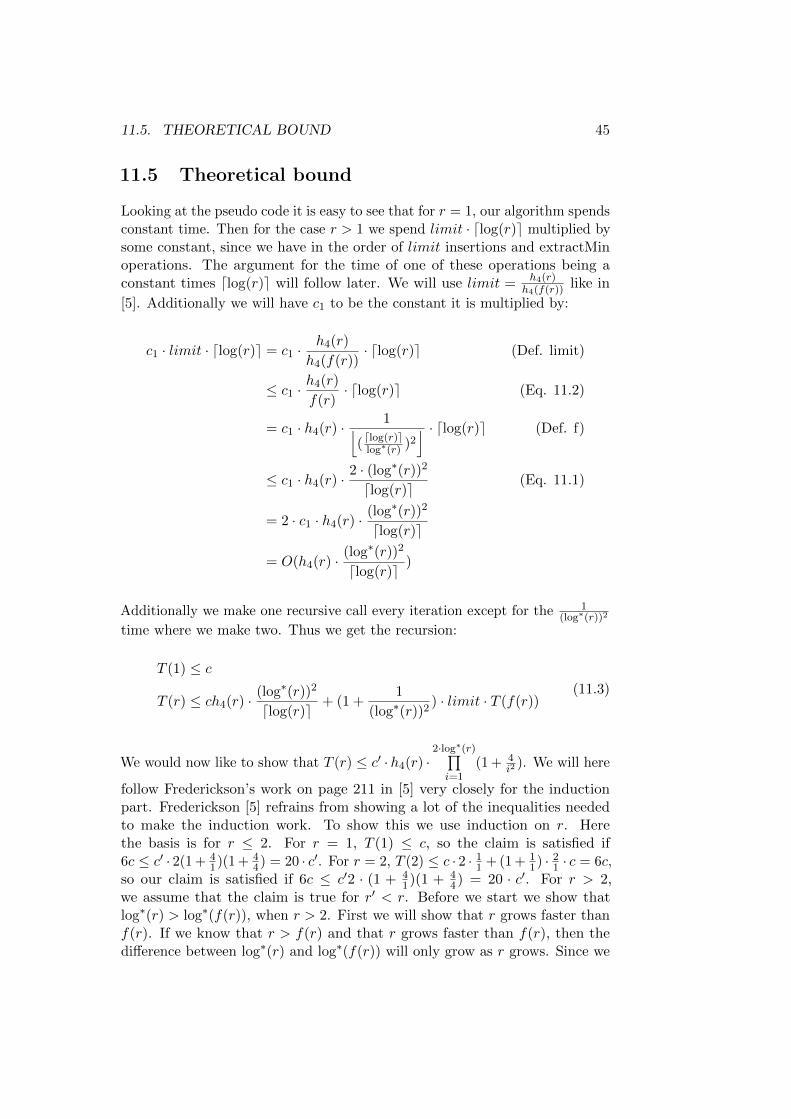
11.5 Theoretical bound
Looking at the pseudo code it is easy to see that for r = 1, our algorithm spendsconstant time. Then for the case r > 1 we spend limit · dlog(r)e multiplied bysome constant, since we have in the order of limit insertions and extractMinoperations. The argument for the time of one of these operations being aconstant times dlog(r)e will follow later. We will use limit = h4(r)
h4(f(r))like in
[5]. Additionally we will have c1 to be the constant it is multiplied by:
c1 · limit · dlog(r)e = c1 ·h4(r)
h4(f(r))· dlog(r)e (Def. limit)
≤ c1 ·h4(r)
f(r)· dlog(r)e (Eq. 11.2)
= c1 · h4(r) · 1⌊( dlog(r)elog∗(r) )2
⌋ · dlog(r)e (Def. f)
≤ c1 · h4(r) · 2 · (log∗(r))2
dlog(r)e(Eq. 11.1)
= 2 · c1 · h4(r) · (log∗(r))2
dlog(r)e
= O(h4(r) · (log∗(r))2
dlog(r)e)
Additionally we make one recursive call every iteration except for the 1(log∗(r))2
time where we make two. Thus we get the recursion:
T (1) ≤ c
T (r) ≤ ch4(r) · (log∗(r))2
dlog(r)e+ (1 +
1
(log∗(r))2) · limit · T (f(r))
(11.3)
We would now like to show that T (r) ≤ c′ · h4(r) ·2·log∗(r)∏
i=1(1 + 4
i2). We will here
follow Frederickson’s work on page 211 in [5] very closely for the inductionpart. Frederickson [5] refrains from showing a lot of the inequalities neededto make the induction work. To show this we use induction on r. Herethe basis is for r ≤ 2. For r = 1, T (1) ≤ c, so the claim is satisfied if6c ≤ c′ · 2(1 + 4
1)(1 + 44) = 20 · c′. For r = 2, T (2) ≤ c · 2 · 11 + (1 + 1
1) · 21 · c = 6c,so our claim is satisfied if 6c ≤ c′2 · (1 + 4
1)(1 + 44) = 20 · c′. For r > 2,
we assume that the claim is true for r′ < r. Before we start we show thatlog∗(r) > log∗(f(r)), when r > 2. First we will show that r grows faster thanf(r). If we know that r > f(r) and that r grows faster than f(r), then thedifference between log∗(r) and log∗(f(r)) will only grow as r grows. Since we

46 CHAPTER 11. SEL4 O(k)
Table 11.1: r vs. f(r)
r 3.0 4.0 5.0 6.0 7.0 8.0 9.0 10.0 11.0
f(r) 1.0 1.0 1.0 1.0 1.0 1.0 1.0 1.0 1.0
have:
f(r) =
⌊dlog(r)e2
(log∗(r))2
⌋
≤ dlog(r)e2
(log∗(r))2
≤ dlog(r)e2
≤ (1 + log(r))2
The growth of f is smaller than or equal to the growth of (1 + log(r))2. To gethow fast (1 + log(r))2 grows, we take the derivative:
d
dr((1 + log(r))2) = 2 · (log(r) + 1) · 1
r · ln(2)
We also take the derivative of r, but this is simple and we get ddr (r) = 1. In
order for it to hold that:
2 · (log(r) + 1) · 1
r · ln(2)≤ 1
We need to have r ≥ 12. That means for r ≥ 12, r grows faster thanf(r). What is missing then to show that r also grows faster than f(r) forr ∈ {3, 4, 5, 6, 7, 8, 9, 10, 11}. We show them all in Table 11.1. We can see fromTable 11.1 that r also grows faster than f(r) below 12. Since we have establishedthat r grows faster than f(r) we only remain to show that for the smallestpossible difference between r and f(r), it holds that log∗(r) > log∗(f(r)). Thissmallest possible value is for r = 3, since we are only dealing with the casewhere r > 2. We obtain:
log∗(3) = 1 + log∗(2) = 2
log∗(f(3)) = log∗(1) = 1
Since 2 > 1, we obtain:
log∗(r) > log∗(f(r)) (11.4)

11.5. THEORETICAL BOUND 47
Note that this result means that log∗(f(r)) ≤ log∗(r)− 1. Now we will do theinduction case of our proof. We have:
T (r) ≤ ch4(r) · (log∗(r))2
dlog(r)e+ (1 +
1
(log∗(r))2) · h4(r)
h4(f(r))(Eq. 11.3)
≤ ch4(r)(log∗(r))2
dlog(r)e
+ (1 +4
(2 log∗(r))2)
h4(r)
h4(f(r))c′h4(f(r))
2 log∗(f(r))∏i=1
(1 +4
i2) (Ind. Hypo.)
≤ ch4(r)(log∗(r))2
dlog(r)e+ (1 +
4
(2 log∗(r))2)c′h4(r)
2 log∗(r)−2∏i=1
(1 +4
i2) (Eq. 11.4)
= ch4(r)(log∗(r))2
dlog(r)e+
c′h4(r)2 log∗(r)∏
i=1(1 + 4
i2)
(1 + 4(2 log∗(r)−1)2 )
Using the last equation, we can see that it will hold if:
ch4(r)(log∗(r))2
dlog(r)e+
c′h4(r)2 log∗(r)∏
i=1(1 + 4
i2)
(1 + 4(2 log∗(r)−1)2 )
≤ c′ · h4(r) ·2 log∗(r)∏
i=1
(1 +4
i2)
Multiplying by (1 + 4(2 log∗(r)−1)2 ) we obtain:
ch4(r)(log∗(r))2
dlog(r)e(1 +
4
(2 log∗(r)− 1)2) + c′h4(r)
2 log∗(r)∏i=1
(1 +4
i2)
≤ (1 +4
(2 log∗(r)− 1)2)c′h4(r)
2 log∗(r)∏i=1
(1 +4
i2)
The plus one on the right side multiplied with the c′h4(r)2 log∗(r)∏
i=1(1 + 4
i2) on
the right side, eats that same expression on the left side, giving us:
ch4(r)(log∗(r))2
dlog(r)e(1 +
4
(2 log∗(r)− 1)2) ≤ (
4
(2 log∗(r)− 1)2)c′h4(r)
2 log∗(r)∏i=1
(1 +4
i2)
Which finally gives us:
(log∗(r))2
dlog(r)e (1 + 4(2 log∗(r)−1)2 )
( 4(2 log∗(r)−1)2 )
2 log∗(r)∏i=1
(1 + 4i2
)
· c ≤ c′

48 CHAPTER 11. SEL4 O(k)
Figure 11.1: C(r) over r.
Which simplifies to:
(log∗(r))2((2 log∗(r)− 1)2 + 4)
4dlog∗(r)e2 log∗(r)∏
i=1(1 + 4
i2)
· c ≤ c′
If we call the expression on the left side C(r), that is:
C(r) =(log∗(r))2((2 log∗(r)− 1)2 + 4)
4dlog∗(r)e2 log∗(r)∏
i=1(1 + 4
i2)
Just like Frederickson says in [5], this function takes on its maximum in therange r = 17 to r = 32, as illustrated in Figure 11.1. We have attempted toprove that this is the case, but have been unable to do so, Frederickson alsodoes not prove this in [5], but on page 212 just states that this is the case.
At the maximum in Figure 11.1 the value is 1.585, which means we get:
1.585 · c ≤ c′

11.5. THEORETICAL BOUND 49
The claim then follows by induction, with c′ chosen to be 1.585 · c. From theclaim it then follows that T (r) = O(r), since for r > 1 we have:
h4(r) = h4(f(r)) ·⌈
r
h4(f(r))
⌉≤ h4(f(r)) · (1 +
1
h4(f(r)))
≤ r + h4(f(r))
≤ r + h4(f(r))
= 2r
and additionally we have from Theorem 19.0.1 and the fact that:
∞∑i=1
4
i2= 4 ·
∞∑i=1
1
i2
converges by Theorem 19.0.2, that∞∏i=1
(1+ 4i2
) converges, and is thereby bounded
by a constant.What now remains to be shown is that the rank of the representative of our
final extracted clan is O(k). We argue this much like the earlier algorithms:Since we argued earlier that a call to RSEL4 with argument k returns theh4(k) smallest elements in a clan, represented by the representative of the clan,and since the representative is the largest element among them and also sincewe extract these from a priority queue, the rank of the representative of thelast extracted clan will be:
h4(k)
h4(f(k))· h4(f(k)) = h4(k)
Since we have, as argued earlier, that h4(k) ≤ 2 · k, our algorithm runs in totalin O(k) time.
Priority queue size
To give some intuition about how large a priority queue PQ can get at anylevel, assume we start off with an empty PQ. We add t elements and thenreturn PQ to the level above. The level above may choose to split or not tosplit PQ. Suppose we can at most choose not to split it b times. This meanswe can add a total of bt elements to PQ before splitting.
After a split PQ will still retain bt2 elements. If we use the now split PQ
another b times, it will have a total of bt2 + bt elements. After another split
and b uses, it will end up withbt2+bt
2 + bt = bt4 + bt
2 + bt elements.The number of elements in PQ before a split is bounded by the sum
∞∑i=0
bt2i
= 2bt.

50 CHAPTER 11. SEL4 O(k)
If we then use the fact that we will at most add h4(f(r))h4(f(f(r)))
· 1log∗(f(r))2
elements at the level beneath level r, and we will at most add additionalelements corresponding to how often we split during our limit = h4(f(r))
h4(f(f(r)))
iterations. Which means we can maximally choose to not split it log∗(r)2 timeswe obtain the sum:
∞∑i=0
(1
2i· h4(f(r))
h4(f(f(r)))· 1
log∗(f(r))2· log∗(r)2)
Since everything except the 12i
does not contain i, we get:
h4(f(r))
h4(f(f(r)))· 1
log∗(f(r))2· log∗(r)2 ·
∞∑i=0
1
2i
= 2 · h4(f(r))
h4(f(f(r)))· 1
log∗(f(r))2· log∗(r)2
≤ 4 · f(r)
h4(f(f(r)))· log∗(r)2 · 1
log∗(f(r))2(h4(r) ≤ 2r)
≤ 4 · f(r)
f(f(r))· log∗(r)2 · 1
log∗(f(r))2(h4(r) ≥ r)
= 4 · f(r)⌊dlog(f(r))e2log∗(f(r))2
⌋ · log∗(r)2 · 1
log∗(f(r))2(Def. f)
≤ 4 · f(r)
( dlog(f(r))e2
log∗(f(r))2 )− 1· log∗(r)2 · 1
log∗(f(r))2
= 4 · log∗(r)2
(( dlog(f(r))e2
log∗(f(r))2 )− 1) · log∗(f(r))2· f(r)
= 4 · log∗(r)2
dlog(f(r))e2)− log∗(f(r))2· f(r)
For this last expression we will look at the expression:
log∗(r)2
dlog(f(r))e2 − log∗(f(r))2
In this expression when r →∞ log(f(r))2 will dominate the other functionssince log∗ is such a slow growing one. This means the fraction will eventuallyconverge. Which means we can replace it with some constant c (possibly large)and for the numbers until dlog(f()r)e2 > log∗(f(r))2 we can just take themaximum value we would obtain from the original expression as a constant.We then get:
4 · c · f(r) = O(f(r))

11.5. THEORETICAL BOUND 51
Which means the size of our priority queue at the level below has size O(f(r))which means it is linear in size. Since we did this for any random level itfollows that our priority queue will never exceed linear size.
Chapter 12
Examples
12.1 Naive
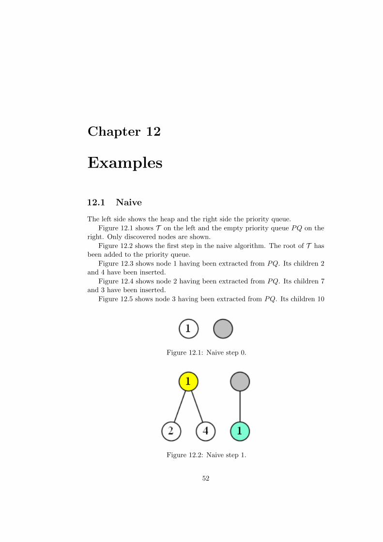
The left side shows the heap and the right side the priority queue.
Figure 12.1 shows T on the left and the empty priority queue PQ on theright. Only discovered nodes are shown.
Figure 12.2 shows the first step in the naive algorithm. The root of T hasbeen added to the priority queue.
Figure 12.3 shows node 1 having been extracted from PQ. Its children 2and 4 have been inserted.
Figure 12.4 shows node 2 having been extracted from PQ. Its children 7and 3 have been inserted.
Figure 12.5 shows node 3 having been extracted from PQ. Its children 10
Figure 12.1: Naive step 0.
Figure 12.2: Naive step 1.
52

12.1. NAIVE 53
Figure 12.3: Naive step 2.
Figure 12.4: Naive step 3.

54 CHAPTER 12. EXAMPLES
Figure 12.5: Naive step 4.
Figure 12.6: SEL1 step 0.
and 12 have been inserted.
The algorithm follows trivially from here, with 4, then 5 being the nextnodes to be extracted.
12.2 SEL1 and SEL2
The left side shows the heap and the right side the priority queue.
Figure 12.6 shows T on the left and the empty priority queue PQ on theright. Only discovered nodes are shown.
Figure 12.7 shows the first clan consisting of the yellow nodes. The clan isfound by a subroutine (naive for SEL1 and SEL2 itself for SEL2), which is not

12.2. SEL1 AND SEL2 55
Figure 12.7: SEL1 step 1.

56 CHAPTER 12. EXAMPLES
Figure 12.8: SEL1 step 2.
shown. The priority queue on the right side contains a single clan with therepresentative 3, members 1, 2, and 3, offspring 7, 10, 11, and 4, and no poorrelation.
Figure 12.8 shows the first clan extracted from PQ, its nodes colored greenin T . From its offspring we’ve created a new clan represented by 6. This clandoes have a poor relation, consisting of 7, 10, and 12.
Note that every node colored white in the heap to the left can be found ineither offspring or poor relation to some clan in the priority queue to the right.
Figure 12.9 shows T after the clan represented by 6 has been extractedfrom PQ. Two new clans have been created, represented by 13 and 10.
Figure 12.10 shows T on the left and the empty priority queue PQ on theright. Only discovered nodes are shown.

12.3. SEL3 AND SEL4 57
Figure 12.9: SEL1 step 3.
12.3 SEL3 and SEL4
The image shows the same two structures for SEL3 and SEL4, but PQ ischanged to reflect its recursive structure. For the example we let k = 8, suchthat for SEL3, log k = 3 and log(log k) = 1. While only SEL3 is depicted, thegeneral idea is the same for SEL4, with the only difference being how large ris at the different levels, how many iterations are made, and when a priorityqueue is split.
The images are colored and may be harder to follow in gray scale. First,to the right we will see three layers of priority queues. We’ll name them afterthe r they’re given, thus from top to bottom, the gray nodes represent PQ8,PQ3 and PQ1. To the left, a white node has been added to a PQ1. A yellow(darker in gray scale) node has been extracted from a PQ1. A green node(darker than the yellow) has been extracted from PQ3. A beige node (brightin gray scale) has been extracted from PQ8.
Figure 12.11 shows T on the left and the empty priority queue PQ on theright.
Figure 12.12 shows a blank PQ8. The recursive call has not returned yet,and there are no clans in it. For PQ3 a clan represented by 1 has been addedto the queue. 1’s children, 2 and 4, are found in the PQ1 belonging to 1. Since1 has been extracted from a PQ1, it has been colored yellow to the left.
Figure 12.13 shows the clan represented by 1 having been extracted fromPQ3. The PQ1 the clan contained has been split into two and recursed on,leaving two new clans in PQ3, represented by 2 and 4. To the left, 1 has been

58 CHAPTER 12. EXAMPLES
Figure 12.10: SEL1 step 4.
Figure 12.11: SEL3 step 0.

12.3. SEL3 AND SEL4 59
Figure 12.12: SEL3 step 1.

60 CHAPTER 12. EXAMPLES
Figure 12.13: SEL3 step 2.

12.3. SEL3 AND SEL4 61
Figure 12.14: SEL3 step 3.
colored green after having been extracted from PQ3 and 2 and 4 have beencolored yellow after extraction from PQ1.
Figure 12.14 shows 2 having been extracted from PQ3 and its PQ1 splitinto 7 and 3 and recursed on. This colors 2 green and 7 and 3 yellow.
Figure 12.15 shows 3 having been extracted from PQ3 and its PQ1 splitinto 10 and 12 and recursed on. This colors 2 green and 7 and 3 yellow. Thisalso concludes the work done in the r = 3 layer, finally adding a clan to PQ8
represented by 3.
Figure 12.16 shows 3 having been extracted from PQ8 and its PQ3 splitinto 7 and 4 on the left and 10 and 12 on the right. We color 3 beige in T , todenote its extraction from PQ8. Node that that level never sees the nodes 1and 2, which are implicitly contained in the clan, thus we leave them green.
To the right, we now have two incomplete clans in PQ8. The exact split ofPQ3 in the implementation might be different. We recurse on the incomplete

62 CHAPTER 12. EXAMPLES
Figure 12.15: SEL3 step 4.
Figure 12.16: SEL3 step 5.

12.3. SEL3 AND SEL4 63
Figure 12.17: SEL3 step 6.
Figure 12.18: SEL3 step 7.
left clan in the next steps.
Figure 12.17 shows recursion on the left incomplete clan in PQ8 (the rightclan has been omitted to save space). This follows the same procedure asabove, extracting 4 from PQ3 and adding 8 and 5. This colors 4 green and 8and 5 yellow.
Figure 12.18 shows 5 having been extracted from PQ3 and 8 and 5 having
64 CHAPTER 12. EXAMPLES
Figure 12.19: SEL3 step 8.
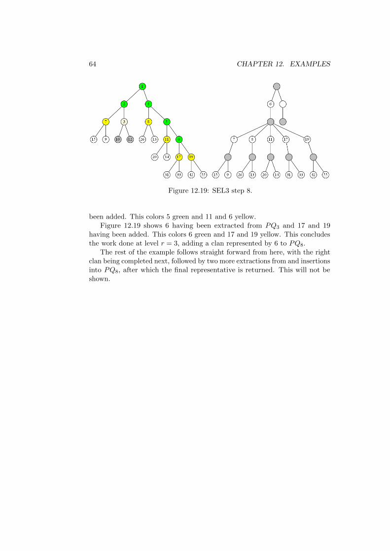
been added. This colors 5 green and 11 and 6 yellow.Figure 12.19 shows 6 having been extracted from PQ3 and 17 and 19
having been added. This colors 6 green and 17 and 19 yellow. This concludesthe work done at level r = 3, adding a clan represented by 6 to PQ8.
The rest of the example follows straight forward from here, with the rightclan being completed next, followed by two more extractions from and insertionsinto PQ8, after which the final representative is returned. This will not beshown.

Chapter 13
SEL4 parameter optimization
13.1 Introduction
In the algorithm SEL4 we have the boundary for when we enter the basecase and the boundary for when we split our priority queues and make tworecursive calls. These two boundaries are 1 and log∗(r)2 respectively fromthe theory. We might improve the running time of our algorithm by slightlychanging these. To do this we have tried out a number of different choices forthe boundary of the base case, we call this value baseCase and the same wehave tried for the other boundary which we call catFactor. Since the choicefor catFactor that optimizes our algorithm might not optimize if we changeour choice of baseCase we have run a cross evaluation with different values forboth our boundaries. We have here chosen to focus on optimality in respect tothe running time of the algorithm. We chose this because we do not know theratio of significance between comparisons and accesses, and the optimal valuesmight differ for these two.
13.2 Choice of Parameters
From Figure 13.1 we can see that around 16 and around 32 our values lookto be minimal. Inspecting the data at these places in Table 13.1 we can seethat our values are in fact minimal with baseCase = 16, catFactor = 0.9 andbaseCase = 32, catFactor = 1.0. Since from Figure 13.1 the region aroundbaseCase = 32 and catFactor = 1.0 looks less rapidly changing than aroundthe other region, we have chosen these as the parameters for SEL4 in ourexperiments.
65

66 CHAPTER 13. SEL4 PARAMETER OPTIMIZATION
Figure 13.1: Graphical representation of the data in Table 13.1. Time is inmicroseconds.
Table 13.1: SEL4 parameter optimization data
0.6 0.7 0.8 0.9 1.0 2.0 3.0 4.0 5.0 6.0
1 1948111 1333077 941053 857049 859050 770044 722041 706040 700040 6980402 980056 921053 887051 857049 855049 837048 840048 847048 752043 7020404 985057 932053 894051 859049 855049 768044 724041 718041 699040 6940398 990057 994057 1051060 1002057 865050 758043 732042 1338076 1392080 81304712 1013057 942054 893051 948055 1004057 898051 736043 713040 700040 69104016 460026 466027 460026 455026 460027 461026 467027 468026 476028 48302720 462027 470027 461026 534031 530030 539031 557032 549031 552032 56103224 533030 534031 534030 535031 520030 461026 468027 469027 473027 48102728 463027 461026 460026 460027 457026 460026 465027 475027 469027 48102732 460027 458026 465026 456026 455026 460027 469027 483027 550032 56403236 535031 535030 535031 530030 531031 549031 543031 547031 551032 56003240 533030 539031 540031 533031 531030 540031 543031 546031 550032 56003250 534030 537031 535030 532031 532030 539031 544031 549032 549031 56203260 533031 536030 533031 531030 529031 538030 553032 548031 548032 559032
The numbers on the top are the numbers we multiplied our theoreticalcategory with, and the numbers on the far left are the numbers that defineour base case. Entries are runtime in microseconds on data size 1000000.

13.2. CHOICE OF PARAMETERS 67
Figure 13.2: Graphical representation of the data in Table. Time is in mi-croseconds. 13.1
Table 13.2: SEL4 parameter optimization data
0.6 0.7 0.8 0.9 1.0 2.0 3.0 4.0 5.0 6.0
1 1001057 993057 989056 995057 990057 991057 1001057 1005057 1011058 10270592 1009058 1009057 999057 1001058 990056 995057 1001058 1001057 1008057 10270594 994057 996057 996057 989057 989056 994057 1015058 1024059 1022058 10360598 999058 997057 989056 997057 988057 991056 1004058 1014058 1010058 102505812 995057 999057 1000058 995057 997057 1006057 1014058 1015058 1016058 102805916 996057 1000057 991057 992057 996057 993057 1002057 1011058 1012058 102605820 995057 999057 1008058 1004057 1014058 997058 1008057 1006058 1016058 102505924 992056 1000058 996056 1001058 988056 996057 1007058 1010058 1020058 103505928 1002058 1009057 1002058 995057 988056 1000057 1006058 1006057 1014058 102805932 997057 998057 998057 999057 996057 999058 1018058 1021058 1021059 103905936 1005058 995056 1001058 1002057 992057 996057 1005057 1014058 1017058 102605940 997057 996057 996057 994057 1004057 1003058 1011058 1025058 1013058 104506050 997057 997057 994057 995057 994057 1004057 1009058 1010058 1015058 102405860 996057 1003058 1006057 1006058 997057 1015058 1007058 1007057 1020059 1027058
The numbers on the top are the numbers we multiplied our theoreticalcategory with, and the numbers on the far left are the numbers that defineour base case. Entries are runtime in microseconds on data size 1000000.

Chapter 14
Experiment heaps
14.1 Worst case
Image 14.1 shows the worst case test heap. The k smallest elements will forma right spine down the tree, and the left child of a node with a value of 1 willhave a high value. The first left child will have a value higher than k (100 inthe example), and its subtree will have the same value. The next left child ofa 1 node will have one lower than the previous. This affects how the naivealgorithm’s internal priority queue shuffles around the nodes.
Looking at the tree, in the naive algorithm the first node we add to thepriority queue PQ is the root. After we extract it, 100 and 1 are added. 1 issmaller than all other elements, so it is forced to traverse PQ all the way fromthe bottom to the top, swapping place with 100 in the internal array.
Next we extract 1, leaving only 100. We add 99, which is smaller than 100,and is thus moved to the front of the array. Then 1 is added, which again hasto be moved all the way to the front.
Once we extract 1 again, we are left with 100 and 99. We first add 98 andthen 1, both of which have to the moved all the way from the back to the front.This continues until k elements have been extracted and 2 ·k elements inserted,each insertion taking the worst case number of operations to complete.
14.2 Random case
The random case tree is an infinite tree where every node has a value equal tothe value of their parent plus a random number in the range [1, 100]. Theserandom numbers were generated using std::uniform int distribution fromthe Standard Template Library.
We expect the Random Case to be a slightly worse case than the BestCase, but not by a lot. The reason we have this expectation is becauseinserting random elements into a priority queue will by expectation not movethe elements around a lot.
68

14.3. BEST CASE 69
Figure 14.1: Worst case heap.
For our testing of the Random Case we should note that we have left outalgorithm SEL2, because we disabled the Selection part of the algorithms, andwithout this SEL2 does not work at all. The reason for this is that since weare using random numbers the Selection part will vary by a lot on how muchtime it spends on this part, and therefore our results would be hard to explain.Additionally our experimental testing of the Selection algorithm indicated thatwe could not necessarily trust that it was linear time.
14.3 Best case
The best case tree is one where all nodes have the same value. Insertion andextraction of nodes never cause any swapping of nodes. In the implementationall nodes have the value 1.

70 CHAPTER 14. EXPERIMENT HEAPS
This makes the naive algorithm linear, as insertions and extractions arenow constant time operations.
It did not work as expected, see Chapter 15.

Chapter 15
Priority Queue Trouble
In our priority queues we have relied on std::priority queue as mentionedearlier. We expected this implementation on insertions to insert the insertedelement into the bottom right most part of the tree, and then bubble the elementup through the tree until it has found its correct position. For extractMin(called pop), we expected it to remove the root, then insert the bottom rightmost element into the root and bubble that element down until it found itscorrect position.
It is with this in mind we created our test cases. That is why when insertingonly elements with the same value we would expect the insert operation tobe constant time, since we will not need to bubble any elements around. Weexpected the same for extraction. Essentially, the bubble up and bubble downprocedures should be constant time.
Looking at Figure 15.1 we see no indication that the insert operation is notconstant as expected. We get two jumps, one at k = 213 and one at k = 220.The machine that ran the test had 32 KB L1 data cache. The elements insertedin the test each take up 4 B, leaving room for:
32 · 1024
4= 213
The machine also had 4 MB L3 data cache, leaving room for:
4 · 1024 · 1024
4= 220
Incidentally, the two most noticeable jumps are at k = 213 and k = 220
in Figure 15.1. Before, between, and after these peaks it looks reasonablyconstant.
If we look at Figure 15.2, the extractMin operation does not look veryconstant. Outside of the k = 220 L3 data cache jump, it looks like a growinglinear function. This could be an indication of a O(n · log n) bound, where nis the number of elements in the priority queue.
71

72 CHAPTER 15. PRIORITY QUEUE TROUBLE
Figure 15.1: Insertions into std::priority queue divided by k over log k.Every element inserted had value 1.
Figure 15.2: Pops from std::priority queue divided by k over log k. Everypopped element had value 1.

73
This seem to indicate that the pop operation does not work as expected. Ad-ditionally we had a look into the GCC (GNU Compiler Collection, gcc.gnu.org)implementation, which is the one we use, and while we do not fully understandhow it works, it definitely does not work according to our original expectation.
This insight came late during the project, and unfortunately we did nothave the time to write our own version, insert it everywhere, and rerun all thetests.

Chapter 16
Experimental results
16.1 System specification
The system used to run the tests was rented on Amazon Web Services(aws.amazon.com) where it was named m4.xlarge. It had the following specs:
• Architecture: x86 64
• Clock speed: 2394 MHz
• CPUs: 8
• RAM: 16 GB
• L1 instruction cache: 32KB
• L1 data cache: 32KB
• L2 data cache: 256KB
• L3 data cache: 30 MB
• Operating system: Ubuntu 14.04 LTS
16.2 Runtime
Runtime was measured in microseconds using std::chrono::high resolution
clock from the Standard Template Library. Runtimes that measured below100,000 microseconds were run again as follows:
1. begin := now()
2. rounds := 1
3. completed := 0
74

16.2. RUNTIME 75
4. time := 0
5. Loop:
a) Run algorithm.
b) completed := completed + rounds
c) rounds := rounds ∗ 2
d) time := now()− begin
e) If time > 100000:
i. time := timecompleted
ii. Break.
Essentially, the benchmark continuously doubled the number of times analgorithm was run until it took at least 100,000 microseconds, then divided thetotal time by the total number of runs. This was done to scale up the fastestbenchmarks and make them measurable.
The number of extra runs grows exponentially, to reduce the overhead ofchecking if enough time had passed.
For the runtime tests, the fastest of five runs was kept. The rationale isthat many things can contribute noise to the runtime result, but almost noneof that noise make the runtime faster. The ticking clock can have a significanteffect, if for instance the start and end measurements happen to be the same,the total time is 0. However, this affects the shorter runtimes the most andwas mitigated with the extra runs described above.
Worst case
Figure 16.1 shows the runtime of all five algorithms in microseconds dividedby k over log k. Just like before, SEL2 and partly SEL3 are the slowest. Ajump is visible in both at 216, where an extra layer of recursion is added.Both are otherwise horizontal, which implies a linear growth, aside from whenlog∗ changes value. This is because a time complexity of O(k · 3log∗ k) ispractically linear. log∗ increases in increments of one at the values 22 = 22 = 4,32 = 24 = 16, and 42 = 216 = 65536. The next increment will be at 52 = 265536,which is way outside of practical reach.
Figure 16.2 shows the runtime of the three fastest algorithms in microsec-onds divided by k over log k. With the noise of the slower algorithms cut out,we can see both SEL1 and SEL4 become horizontal as k grows. SEL1’s timecomplexity is O(k · log log k), which is practically indistinguishable from O(k):For input size below 232, log log k never exceeds 5. If we increase the inputsize to 264, we only increase log log k to 6.
Naive is not horizontal due to log k not being insignificant in the data sizeswe’re able to test. The test design ensures that the internal priority queue

76 CHAPTER 16. EXPERIMENTAL RESULTS
Figure 16.1: Runtime in microseconds divided by k over log k. Worst case tree.
Figure 16.2: Runtime in microseconds divided by k over log k. Worst case tree.

16.2. RUNTIME 77
Figure 16.3: Runtime in microseconds divided by k · log k over log k. Worstcase tree.
used by the naive algorithm always exhibits its worst case time complexity,see chapter 14. At k = 220 SEL4, with its linear complexity, starts beating thenaive algorithm in execution time.
Figure 16.3 shows the naive algorithm with runtime in microseconds dividedby the theoretical bound of O(k · log k). It does not form a horizontal line.Figure 17.10 shows the L3 data cache misses for the naive algorithm, whichstabilizes at around k = 220. The runtime graph also stabilizes at that point,and it is likely that cache misses are to blame for the increase in runtime beforek = 220. This supports that the theoretical bound holds for the implementation.
Random case
As mentioned in 14, SEL2 is not run in any of the tests with the random casegraph.
Figure 16.4 shows the runtime of the four algorithms in microsecondsdivided by k over log k. Like the worst case tree, SEL3 is the slowest, butotherwise appears linear outside of k = 216.
Figure 16.5 shows the runtime of the three fastest algorithms in microsec-onds divided by k over log k. In comparison to the worst case tree in Figure16.2, SEL4 climbs from 216 to 224. Some of this can be explained by more L3data cache misses, which can be seen in Figure 17.21. The test worst case treehas fewer L3 data cache misses, while the random tree has more. The naivealgorithm also performs better on random data compared to a tree that wascreated to get worst case performance on all operations the naive algorithmrelies on.

78 CHAPTER 16. EXPERIMENTAL RESULTS
Figure 16.4: Runtime in microseconds divided by k over log k. Random tree.
Figure 16.5: Runtime in microseconds divided by k over log k. Random tree.

16.2. RUNTIME 79
Figure 16.6: Runtime in microseconds divided by k · log k over log k. Randomtree.
Figure 16.6 shows the naive algorithm with runtime in microseconds dividedby the theoretical bound of O(k · log k). Like the worst case graph, it does notform a horizontal line before k = 221. Figure 17.21 shows the L3 data cachemisses for the naive algorithm, which starts to flatten at k = 222. From thiswe can attribute some of the growth before k = 221 to increasing L1 and L3data cache misses.
Best case
Figure 16.7 shows the runtime of all five algorithms in microseconds dividedby k over log k. Like the worst case tree, SEL2 and SEL3 are the slowest, andappear otherwise linear outside of k = 216.
Figure 16.8 shows the runtime of the three fastest algorithms in microsec-onds divided by k over log k. In comparison to the worst case tree in Figure16.2, SEL4 has some climb from 215 to 217, but remains constant otherwise.
SEL1 climbs from 215 to 219 and again climbs around 222. Outside of thoseregions it remains mostly constant.
The naive algorithm does not appear constant. An array based priorityqueue can be inserted into and extracted from in constant time when allelements are equal. Something affects the runtime, but unfortunately we donot know what.
The naive algorithm is faster than SEL4 for all data points we collected.The missing data points for SEL1 and SEL4 are due to the machine runningout of memory on the best case tree earlier than on the worst case tree.

80 CHAPTER 16. EXPERIMENTAL RESULTS
Figure 16.7: Runtime in microseconds divided by k over log k. Worst case tree.
Figure 16.8: Runtime in microseconds divided by k over log k. Best case tree.

16.3. COMPARISONS 81
Figure 16.9: Runtime in microseconds divided by k · log k over log k. Best casetree.
Figure 16.9 shows the naive algorithm with runtime in microseconds dividedby the theoretical bound of O(k · log k). Like the worst case graph, it does notform a horizontal line. Figure 17.32 shows the L3 data cache misses for thenaive algorithm, but it does not help explain the growth.
16.3 Comparisons
Comparisons were measured only in a single run, since any random numberswere created from a fixed seed and the algorithms are otherwise deterministic.
Worst case
Figure 16.10 shows horizontal lines for SEL2 and SEL3, except for k = 216.
Figure 16.11 shows SEL1 and SEL4 are less horizontal than SEL2 andSEL3. It’s hard to say if they converge. Naive clearly does not converge onthe graph, which supports its O(k · log k) bound.
Random case
Figure 16.12 shows horizontal line for SEL3, except for k = 216.
Figure 16.13 shows SEL1 and SEL4 are very close to horizontal lines.Compared to Figure 16.11, all three algorithms appear to have a lower overhead.This is likely caused by the operation of inserting a random element into apriority queue not always being log of the size of the queue.

82 CHAPTER 16. EXPERIMENTAL RESULTS
Figure 16.10: Comparisons divided by k over log k. Worst case tree.
Figure 16.11: Comparisons divided by k over log k. Worst case tree.

16.3. COMPARISONS 83
Figure 16.12: Comparisons divided by k over log k. Random tree.
Figure 16.13: Comparisons divided by k over log k. Random tree.

84 CHAPTER 16. EXPERIMENTAL RESULTS
Figure 16.14: Comparisons divided by k over log k. Best case tree.
Figure 16.15: Comparisons divided by k over log k. Best case tree.
Best case
Figure 16.14 shows horizontal lines for SEL2 and SEL3, except for k = 216.
Figure 16.15 shows SEL1 and SEL4 are considerably closer to horizontallines than in Figure 16.11. The naive algorithm is still not horizontal, butit has much smaller values than in the worst case tree. SEL4 makes more

16.4. ACCESSES 85
Figure 16.16: Accesses divided by k over log k. Worst case tree.
comparisons than in the worst case tree, while SEL1 remains the same.
16.4 Accesses
Accesses were measured only in a single run, since any random numbers werecreated from a fixed seed and the algorithms are otherwise deterministic.
Worst case
Figure 16.16 shows SEL2 being close to linear with respect to the number ofaccesses, again except for k = 216.
Figure 16.17 shows the number of accesses done by the naive algorithm,SEL1, SEL3, and SEL4 divided by k. SEL3 is horizontal outside of k = 216
and SEL4 is horizontal all the way. It’s hard to say if SEL1 converges, whilethe naive clearly does not.
Figure 16.18 shows the naive algorithm with accesses and comparisonsdivided by the theoretical bound of O(k · log k). Both comparisons and accessesseem to be constant, supporting the theoretical bound.
Random case
Figure 16.19 shows horizontal lines for SEL3, except for k = 216. SEL1 andSEL4 also seem mostly horizontal. Note that compared to Figure 16.17, theoverhead of all but SEL4 are much lower. This is likely part of the reason the

86 CHAPTER 16. EXPERIMENTAL RESULTS
Figure 16.17: Accesses divided by k over log k. Worst case tree.
Figure 16.18: Accesses and comparisons divided by k · log k over log k. Worstcase tree.

16.4. ACCESSES 87
Figure 16.19: Accesses divided by k over log k. Random tree.
Figure 16.20: Accesses and comparisons divided by k · log k over log k. Randomtree.
SEL4 does not get faster than the naive algorithm in the tests. See Figure16.5.
Figure 16.20 shows the naive algorithm with accesses and comparisonsdivided by the theoretical bound of O(k · log k). Like the worst case graph,both comparisons and accesses seem to be constant, supporting the theoreticalbound.

88 CHAPTER 16. EXPERIMENTAL RESULTS
Figure 16.21: Accesses divided by k over log k. Best case tree.
Figure 16.22: Accesses divided by k over log k. Best case tree.
See Figure 16.6 for the timing.
Best case
Figure 16.21 shows horizontal lines for SEL2 and SEL3, except for k = 216.Figure 16.22 shows a horizontal line for SEL4, and a near horizontal line
for SEL1. The naive algorithm appears to do more than a linear number of

16.5. CONCLUSION 89
Figure 16.23: Accesses and comparisons divided by k · log k over log k. Bestcase tree.
accesses, despite the shape of the best case tree. We can not give a reasonablecause for that, however.
Compared to Figure 16.17, SEL4 does almost three times as many accessesand the naive algorithm does starts lower and grows at a slower pace.
Figure 16.23 shows the naive algorithm with accesses and comparisonsdivided by the theoretical bound of O(k · log k). Like the worst case graph,both comparisons and accesses seem to be constant, supporting the theoreticalbound.
16.5 Conclusion
Worst case
SEL4 is the fastest algorithm when k gets large enough. It also has the lowestnumber of accesses and comparisons. The naive algorithm is the second fastest,with SEL1 following closely behind.
SEL2 and SEL3 both seem to follow their theoretical time complexity veryclosely: SEL2 with the bound of O(k · 3log∗(k)) seem to increase its number ofaccesses, comparisons, and its runtime by a factor of 3 at k = 216, which iswhere log∗ jumps from 4 to 5. Similarly SEL3, with its theoretical bound ofO(k · 2log∗(k)) seem to double its accesses, comparisons, and runtime at thesame point.

90 CHAPTER 16. EXPERIMENTAL RESULTS
Random case
SEL4 gets performs poorly and never catches up to SEL1 or the naive algorithm.Some of the issues can be attributed to data cache misses being more frequentthan in the worst case tree tests.
The naive algorithm performs well on random data. SEL1 starts off worse,climbs with its L3 data cache misses, and ends up being as fast as the naivealgorithm at the end.
Best case
The naive algorithm is the fastest, though it looks like if more data pointsexisted for SEL4, they might have been on par at k = 225. This was expected,though the naive algorithm was also expected to be linear, which it is not onthe runtime graphs. This is explained in Chapter 15.
SEL1, SEL2, SEL3, and SEL4 behave largely the same way as in the worstcase.

Chapter 17
Valgrind Results
The Linux tool Valgrind was used to profile the implementations in terms of thenumber of instructions used, the number of memory lookups, and the numberof L1 and L3 data cache misses. Valgrind is also able to profile branchesand branch mispredicts. However, due to time constraints the tests have notbeen instrumented with a branch simulator. Branch simulation is very timeconsuming, and without it some tests already ran for over 20 hours.
Valgrind is available at valgrind.org
Figure 17.1: Instruction references divided by k over log k. Worst case tree.
91

92 CHAPTER 17. VALGRIND RESULTS
Figure 17.2: Data references divided by k over log k. Worst case tree.
Figure 17.3: Instruction references divided by k over log k. Worst case tree.
17.1 Worst case
Figure 17.1 shows instruction references over log k. Figure 17.2 shows datareferences over log k. Both are very similar graphs to Figure 16.1 and showthat runtime of SEL2 and SEL3 are mostly determined by the number ofinstruction they use and the number of data references they make.

17.1. WORST CASE 93
Figure 17.4: Data references divided by k over log k. Worst case tree.
Figure 17.5: Instructions and data references divided by k · log k over log k.Worst case tree.
Figure 17.3 shows instruction references over log k for the fastest threealgorithms. Figure 17.4 shows data references over log k for the same algorithms.Both are similar. SEL1 and SEL4 appear mostly constant in both graphs.The naive algorithm appears to climb, though it is uses less instructions andreferences memory less than SEL4 does for all data points.

94 CHAPTER 17. VALGRIND RESULTS
Figure 17.6: L1 data cache misses divided by k over log k. Worst case tree.
Figure 17.7: L1 data cache misses divided by k over log k. Worst case tree.
Figure 17.5 shows the number of instructions and data references usedby the naive algorithm divided by k · log k. They both seem to converge andsupport that the implementation follows the theoretical bound.
Figure 17.6 shows L1 data cache misses divided by k for all five algorithms.SEL3 appears mostly constant after it settles after k = 216. SEL2 does nothave enough data points to support any conclusions.
Figure 17.7 shows the same for the naive algorithm, SEL1, and SEL4. All

17.1. WORST CASE 95
Figure 17.8: L1 data cache missrate over log k. Worst case tree.
three appear mostly constant, and again the naive algorithm has less L1 datacache misses than SEL4.
Figure 17.8 shows the L1 data cache missrate for all five algorithms. SEL2has a noteworthy small missrate. This can be explained by SEL2 computingthe same clans many times over, where the cache is already filled with thedata needed for the next calculations.
At the top of the graph, SEL3 has the highest L1 missrate. SEL3 guaranteesclans are returned at most once from any level of RSEL3, making it less likelyfor data it needs to be in the L1 cache. Still the missrate is below 3% for allfive algorithms.
The naive algorithm seems to steadily drop its missrate from 2.5% atk = 210 to below 1.5% at k = 225. This can be explained by the worst casetree forcing the array based priority queue of the naive algorithm to performthe maximum number of swaps for every insertion and extraction. In anarray based priority queue, most of these swaps will involve nodes at the top,meaning at the front of the array, which will be in cache. Early in the dataset, where k is small, the O(k · log k) operations performed by the priorityqueue is not much larger than the O(k) lookups into the tree H0. Later, asthe log k factor starts to set in, more time will be spent in the priority queuethan getting elements from H0.
SEL1 and SEL4 appear mostly constant.
Figure 17.9 shows L3 data cache misses divided by k for all five algorithms.SEL2 and SEL3 around k = 214 and k = 216. After that SEL3 appears constant,while SEL2 does not have enough data points to support any conclusions.
Figure 17.10 shows the same for the naive algorithm, SEL1, and SEL4. All

96 CHAPTER 17. VALGRIND RESULTS
Figure 17.9: L3 data cache misses divided by k over log k. Worst case tree.
Figure 17.10: L3 data cache misses divided by k over log k. Worst case tree.

17.2. RANDOM CASE 97
Figure 17.11: L3 data cache missrate over log k. Worst case tree.
three appear mostly constant, and again the naive algorithm has less L3 datacache misses than SEL4, just like it did with L1 data cache misses.
Figure 17.11 shows the L3 data cache missrate over log k for all five algo-rithms. Like for L1 misses, SEL3 is the highest and starts spiking at k = 214.This conforms with the high memory use of SEL3, making it fill up the L3cache earlier than the other algorithms.
SEL2 is barely visible at the bottom. The naive algorithm, SEL1, andSEL4 seem to converge. The naive algorithm again has a lower missrate thanSEL4.
17.2 Random case
As mentioned in 14, SEL2 is not run in any of the tests with the random casegraph.
Figure 17.12 shows instruction references over log k. Figure 17.13 showsdata references over log k. Both are very similar graphs to Figure 16.1 andshow that runtime of SEL3 is likely determined by the number of instructionit uses use and the number of data references it makes.
Figure 17.14 shows instruction references over log k for the fastest threealgorithms. Figure 17.15 shows data references over log k for the same algo-rithms. They are similar. SEL4 appears mostly constant in both graphs, whileSEL1 appears to converge. The naive algorithm climbs, though at a muchslower rate than seen in Figure 17.3. Random numbers inserted into an arraybased priority queue is expected to be better than the worst case, and it showsin the slower climb.

98 CHAPTER 17. VALGRIND RESULTS
Figure 17.12: Instruction references divided by k over log k. Random tree.
Figure 17.13: Data references divided by k over log k. Random tree.

17.2. RANDOM CASE 99
Figure 17.14: Instruction references divided by k over log k. Random tree.
Figure 17.15: Data references divided by k over log k. Random tree.

100 CHAPTER 17. VALGRIND RESULTS
Figure 17.16: Instructions and data references divided by k · log k over log k.Random tree.
Figure 17.17: L1 data cache misses divided by k over log k. Random tree.
Figure 17.16 shows the number of instructions and data references used bythe naive algorithm divided by k · log k. Like the worst case graph, they bothseem to converge and support that the implementation follows the theoreticalbound.
Figure 17.17 shows L1 data cache misses divided by k for all five algorithms.SEL3 appears mostly constant after it settles after k = 216.

17.2. RANDOM CASE 101
Figure 17.18: L1 data cache misses divided by k over log k. Random tree.
Figure 17.19: L1 data cache missrate over log k. Random tree.
Figure 17.18 shows the same for the naive algorithm, SEL1, and SEL4. Allthree appear to converge, with SEL4 having about 50% more L1 data cachemisses than the naive algorithm and SEL1.
Figure 17.17 shows the L1 data cache missrate of the four algorithms. Thenaive algorithm tops at around k = 215 and then declines. The other threeremain constant throughout.
Note that while the naive algorithm has a higher L1 data cache missrate

102 CHAPTER 17. VALGRIND RESULTS
Figure 17.20: L3 data cache misses divided by k over log k. Random tree.
Figure 17.21: L3 data cache misses divided by k over log k. Random tree.
than SEL4, SEL4 has more misses since it has more data references. SimilarlySEL1 has the lowest missrate, but the highest number of data referencesamongst the three.
Figure 17.20 shows the L3 data cache misses divided by k of the fouralgorithms. SEL3 converges after the jump.
Figure 17.21 shows the L3 data cache misses divided by k of the threefastest algorithms. All three perform similar climbs, but SEL4 ends up having

17.3. BEST CASE 103
Figure 17.22: L3 data cache missrate over log k. Random tree.
around one third more L3 data cache misses than the naive algorithm andSEL1.
Figure 17.22 shows the L3 data cache missrate for all four algorithms. SEL3spikes much earlier than the other three due to its higher memory usage. Thenaive algorithm has the highest misrate at 8%, but since SEL4 has many moredata references, it also has more L3 data cache misses, as seen in Figure 17.21.
In general, the naive algorithm’s superior performance can be attributedto its priority queue performing much better at random data than worst casedata. The worst case tree also had an L3 data cache missrate that convergedmuch earlier, beginning at k = 218, see Figure 17.11. In comparison, the sametest on the random tree doesn’t begin to converge before k = 223, giving usvery little data to work with.
17.3 Best case
Figure 17.23 shows instruction references over log k. Figure 17.24 shows datareferences over log k. Both are very similar graphs to Figure 16.1 and showthat runtime of SEL2 and SEL3 are mostly determined by the number ofinstruction they use and the number of data references they make.
Figure 17.25 shows instruction references over log k for the fastest three al-gorithms. Figure 17.26 shows data references over log k for the same algorithms.They are similar. SEL1 and SEL4 appear mostly constant in both graphs.Interestingly, the naive algorithm does not appear constant in instructioncount, likely because the priority queue it uses does not behave as expected.This is discussed further in Chapter 15.

104 CHAPTER 17. VALGRIND RESULTS
Figure 17.23: Instruction references divided by k over log k. Best case tree.
Figure 17.24: Data references divided by k over log k. Best case tree.

17.3. BEST CASE 105
Figure 17.25: Instruction references divided by k over log k. Best case tree.
Figure 17.26: Data references divided by k over log k. Best case tree.

106 CHAPTER 17. VALGRIND RESULTS
Figure 17.27: Instructions and data references divided by k · log k over log k.Best case tree.
Figure 17.28: L1 data cache misses divided by k over log k. Best case tree.
Figure 17.27 shows the number of instructions and data references used bythe naive algorithm divided by k · log k. Like the worst case graph, they bothseem to converge and support that the implementation follows the theoreticalbound.
Figure 17.28 shows L1 data cache misses divided by k for all five algorithms.SEL3 appears mostly constant after it settles after k = 216. SEL2 is too hard

17.3. BEST CASE 107
Figure 17.29: L1 data cache misses divided by k over log k. Best case tree.
Figure 17.30: L1 data cache missrate over log k. Best case tree.
to make sense of with the data available.
Figure 17.29 shows the same for the naive algorithm, SEL1, and SEL4.SEL1 and SEL4 appear mostly constant, while the naive algorithm climbsafter k = 216. See Chapter 15 for an explanation.
Figure 17.28 shows the L1 data cache missrate of the five algorithms. Unlikethe worst case results from Figure 17.28, the naive algorithm deviates from aconstant around k = 216, and climbs to a 18% L1 missrate. SEL4 jumps from

108 CHAPTER 17. VALGRIND RESULTS
Figure 17.31: L3 data cache misses divided by k over log k. Best case tree.
Figure 17.32: L3 data cache misses divided by k over log k. Best case tree.
2% in the worst case graph to 5% here. The remaining algorithms perform asbefore.
Both the naive algorithm and SEL4 performing unexpected is explained inChapter 15.
Figure 17.31 shows a constant SEL3 after the jump and a SEL2 that doesnot come with enough data for analysis.
Figure 17.32 shows SEL1 being close to the same as in Figure 17.32, in

17.4. CONCLUSION 109
Figure 17.33: L3 data cache missrate over log k. Best case tree.
the worst case graph. SEL4 has more L3 cache misses than in the worst casegraph, and the naive algorithm has much fewer.
Figure 17.33 shows the L3 data cache missrate for all five algorithms, thesame as Figure 17.11 shows for the worst case graph. The only difference isthat SEL4 have a much higher missrate. See Chapter 15.
17.4 Conclusion
Worst case
Runtime results for all five algorithms from Chapter 16 largely correlate withinstruction, data reference, and cache data found with Valgrind. SEL2 andSEL3 show linear number of used instructions, data references, and L1 and L3data cache misses, outside of their jump at k = 216, which is where an extralayer of recursion is added.
SEL1 and SEL4 are largely linear in most in most graphs. The naivealgorithm shows linear tendencies in cache related measures, and superlineartendencies in terms of instructions used and data references made.
Random case
The random case tree favors the naive algorithm to the extend that it is thefastest in the tests. It is possible it would eventually lose due to its highercomplexity, but that is speculation.

110 CHAPTER 17. VALGRIND RESULTS
Best case
The best case graphs shows mostly the same as the worst case graphs, due toissues explained in Chapter 15. Some algorithms have switched positions incomparison to one another, with especially SEL4 performing worse. SEL2 ismostly unaccounted for due to lack of data.

Chapter 18
Conclusion
The optimal O(k) algorithm SEL4 presented by Frederickson [5] and describedin Chapter 11 can be faster than the simpler naive algorithm described inChapter 3. SEL2 and SEL3 generally have terrible performance, while SEL1has comparable performance to SEL4 and the naive algorithm.
For the test heap created to give the naive algorithm the worst caseperformance, SEL4 hinted at a practical linear complexity, becoming fasterthan the naive algorithm for k ≥ 220. SEL1 is slower than both SEL4 and thenaive algorithm.
When tested with a random heap, the naive algorithm performed betterthan SEL4. SEL4 was mostly slowed down by cache misses, which only startedto stabilize at k = 223. The machine running the tests could not handle muchlarger than k = 225, so data showing a possible linear performance of SEL4could not be obtained. SEL1 managed to tie with the naive algorithm at thelast data points.
For the best case heap the naive algorithm was faster than SEL4, thoughthe naive algorithm was not linear as expected. The reason for that is explainedin Chapter 15. Judging by the time graph, it is likely SEL4 would be as fastas the naive with a few more data points. SEL1 performed on par with SEL4for some time, then got slower at k ≥ 222.
111

Chapter 19
Theorems
Theorem 19.0.1 (Product convergence) Let an be a sequence of positivenumbers for which an → 0 for n→∞, then the product:
∞∏n=1
(1 + an)
converges if and only if, the sum:
∞∑n=1
an
converges.Proof:For this section whenever we write log we use the natural logarithm. First weshow that:
limx→0
log(1 + x)
x= 1
Since when x = 0, we have log(1) = 0 the fraction will be 00 which is indeter-
minate, we can use L’Hopital’s rule:
limx→0
log(1 + x)
x= lim
x→0
ddx(log(1 + x))
ddx(x)
= limx→0
11+x
1
= limx→0
1
1 + x
= 1
Now we have this we apply the natural logarithm to our product:
log(∞∏n=1
(1 + an)) =∞∑n=1
log(1 + an)
112

113
Remember we have an → 0 for n→∞, we obtain:
liman→∞
log(1 + an)
an= 1
By the limit comparison test we obtain, that∞∑n=1
log(1 + an) converges if and
only if∞∑n=1
an converges.
Theorem 19.0.2 (Sum convergence) The sum:
∞∑i=1
1
i2(19.1)
converges.Proof:If instead of starting the sum of Equation 19.1 in 1 we start it in 2 we obtain:∑
i = 2∞1
i2
Which clearly will also converge if Equation 19.1 does. We then make theobservation that 0 ≤ 1
i2≤ 1
i2−i , since subtracting below from the denominatorwill make the expression bigger. Additionally we show that, for i ≥ 2:
1
i− 1− 1
i=
i− (i− 1)
i · (i− 1)=
1
i2 − i
Using this we can now look at the sum:
∞∑i=2
(1
i− 1− 1
i)
First we will look at the function if rather than going to infinity it goes to someN :
N∑i=2
(1
i− 1− 1
i) = (
1
1− 1
2) + (
1
2− 1
3) + (
1
3− 1
4) + . . . + (
1
N − 2− 1
N − 1) + (
1
N − 1− 1
N)
=1
1− 1
N
We get this because for every part except the first and last there is both apositive and negative occurrence, and these cancel out. If we now let N →∞and look at the limit we get:
limN→∞
N∑i=2
(1
i− 1− 1
i) = lim
N→∞(1− 1
N) = 1
Which means it converges, and thus our original expression of Equation 19.1converges.

Bibliography
[1] Manuel Blum et al. “Time bounds for selection”. In: Journal of Computerand System Sciences 7.4 (Aug. 1973), pp. 448–461. issn: 00220000. doi:10.1016/S0022-0000(73)80033-9. url: http://www.sciencedirect.com/science/article/pii/S0022000073800339.
[2] Gerth Stølting Brodal and Allan Grønlund Jørgensen. “Selecting Sums inArrays”. In: Algorithms and Computation: 19th International Symposium,ISAAC 2008, Gold Coast, Australia, December 15-17, 2008. Proceedings.Ed. by Seok-Hee Hong, Hiroshi Nagamochi, and Takuro Fukunaga. Berlin,Heidelberg: Springer Berlin Heidelberg, 2008, pp. 100–111. isbn: 978-3-540-92182-0. doi: 10.1007/978- 3- 540- 92182- 0_12. url: http:
//dx.doi.org/10.1007/978-3-540-92182-0_12.
[3] Thomas H Cormen et al. Introduction to Algorithms, Third Edition. 3rd.The MIT Press, 2009. isbn: 0262033844, 9780262033848.
[4] David Eppstein. “Finding the k Shortest Paths”. In: SIAM Journal onComputing 28.2 (1998), pp. 652–673. doi: 10.1137/S0097539795290477.eprint: http://dx.doi.org/10.1137/S0097539795290477. url: http://dx.doi.org/10.1137/S0097539795290477.
[5] G.N. Frederickson. “An Optimal Algorithm for Selection in a Min-Heap”.In: Information and Computation 104.2 (June 1993), pp. 197–214. issn:08905401. doi: 10.1006/inco.1993.1030. url: http://www.sciencedirect.com/science/article/pii/S0890540183710308.
[6] J. W. J. Williams. “Algorithm 232 - Heapsort”. In: Communications ofthe ACM 7.6 (1964), pp. 347–348.
114