master thesis - pure.unileoben.ac.at
TRANSCRIPT

MASTER THESISMASTER THESISMASTER THESISMASTER THESIS
Evaluation and comparison of drilling parameters and hardware used to improve cuttings transport and limit the thickness of cuttings accumulations in high angle
and horizontal well bore sections
A thesis submitted to the Mining University of Leoben in partial fulfilment of the requirements for the
Degree of Master of Science in Petroleum Engineering at
the Department of Mineral Resources and Petroleum Engineering
By Trésor SONWA LONTSI B.Sc
Supervised by: Univ.-Prof.-Dipl.-Ing. -Dr.-mont. Gerhard THONHAUSER Dipl.-Ing. Johann SPRINGER
Approval date: June 2008

AFFIDAVIT
I declare herewith that this thesis is entirely my own work and that where any material could
be construed as the work of others, it is fully quoted and referenced.
Tresor Sonwa Lontsi
Leoben, June 2008/ Austri

DEDICATION
This Thesis is dedicated to my parents LONTSI Emmanuel and SOKING Pauline and my
brothers and sister for all their support and encouragement throughout the years. And this
thesis is dedicated also to my fiancée, Cathy PETEGA.

ACKNOWLEDGMENTS
The author would like to express gratitude to Professor Gerhard Thonhauser for his constant
guidance and assistance for the preparation of this thesis.
My deepest thanks go to my technical supervisor Dipl.-Ing. Johann Springer. He has always
been extremely supportive and shared the enthusiasm of working on this interesting project.
Special thank to WEATHERFORD Dubai for providing me with both the technical and
financial support for completing this thesis. I would also like to thank Mr Ramzi Al-Heureithi,
the Vice President of Weatherford in the MENA region and to Mr Harald Bock for their
financial and moral support.
Special thank to the ÖAD for their financial support through the scholarship at the Mining
University in Leoben.
I am extremely grateful to Professor Brigitte Weinhardt for helping me to obtain the subject of
this thesis from Weatherford.
I would like to thank Amadou Rabihou, ex- STURM GRAZ striker for his financial support
during my study. I also would like to thank Fogouh Daniel, Malcolm Werchota for cheering
me up during the hard time in Leoben and all my friends for their help.
Lastly and not the least, I would like to thank GOD for giving me the opportunity to study in
Leoben.

Trésor SONWA LONTSI I
1 Table of Contents
1 Abstract.....................................................................................................................................1
Zusammenfassung............................................................................................................................2
2 Introduction..............................................................................................................................4
3 Objectives and structure of the Thesis.................................................................................6
3.1 Objectives ............................................................................................................................6
3.2 Structure of the thesis..........................................................................................................7
4 Cuttings transport in vertical wellbores ..............................................................................8
4.1 Literature Review................................................................................................................8
4.2 Theory behind the cuttings transport in vertical wells......................................................8 4.2.1 Particle settling mechanisms.......................................................................................9
4.3 Moore Correlation1 ...........................................................................................................11
4.4 Chien Correlation1.............................................................................................................13
4.5 Walker and Mayes correlation1........................................................................................14
5 Cuttings transport in deviated and horizontal wellbores ...............................................15
5.1 Literature Review..............................................................................................................15 5.1.1 First experimental studies .........................................................................................15 5.1.2 Theoretical studies ....................................................................................................17
5.2 Factors influencing the cuttings transport........................................................................19 5.2.1 Annular velocity........................................................................................................20 5.2.2 Wellbore Inclination angle........................................................................................20 5.2.3 Mud Properties ..........................................................................................................21 5.2.4 Drill String Rotation..................................................................................................22 5.2.5 Drilled Cuttings Properties .......................................................................................23 5.2.6 Drill String Eccentricity............................................................................................24 5.2.7 Rate of Penetration....................................................................................................25
5.3 Hole cleaning and cuttings bed formation.......................................................................25 5.3.1 Cuttings bed formation..............................................................................................26 5.3.2 Mode of hole cleaning ..............................................................................................32
5.4 Some methods to determine the bed thickness................................................................33 5.4.1 Empirical correlation using Least Square Method..................................................33 5.4.2 Artificial Neural Network (ANN) 16 ........................................................................35
5.5 Critical angle in deviated wellbores.................................................................................38
5.6 Modes of Cuttings Transport in horizontal section.........................................................40 5.6.1 Wellbore geometry in horizontal interval ................................................................41
5.7 Transport Models used to describe cuttings phenomena................................................42 5.7.1 Model for the prediction of the minimum transport velocity .................................42 5.7.2 New cuttings lifting equation Model4 ......................................................................48 5.7.3 Annular cuttings concentration prediction...............................................................49
6 Drill String Component influencing Cuttings Removal in Deviated wellbore............53
6.1 Well drilled using Standard Drill Pipe.............................................................................53 6.1.1 Field experience ........................................................................................................54 6.1.2 Most related problems with Standard Drill Pipe.....................................................58

Trésor SONWA LONTSI II
6.1.3 Economic evaluation.................................................................................................58
6.2 Wells drilled using HydroClean Drill Pipe......................................................................69 6.2.1 HydroClean................................................................................................................69 6.2.2 Application of HydroClean ......................................................................................76 6.2.3 Field data analysis and result....................................................................................79 6.2.4 Limitations of HydroClean.......................................................................................81 6.2.5 Economic Evaluation................................................................................................81
6.3 Cuttings Bed Impellers......................................................................................................89 6.3.1 Definition of the Cuttings Bed Impellers (CBI) ......................................................89 6.3.2 Applications of the CBI ............................................................................................91 6.3.3 Advantages and Limitations of the CBI...................................................................92
6.4 Helical Drill Pipe...............................................................................................................93 6.4.1 Definition and features..............................................................................................93 6.4.2 Advantages of Helical Drill Pipe..............................................................................94 6.4.3 Limitations of the Helical Drill Pipe........................................................................95
7 Conclusion and Recommendations ....................................................................................96
7.1 Conclusion.........................................................................................................................96
7.2 Recommendations.............................................................................................................97
8 Nomenclatures .......................................................................................................................98
9 References.............................................................................................................................101
10 Appendix...............................................................................................................................104
10.1 Appendix A .................................................................................................................104 10.1.1 Minimum flow rate determination .........................................................................104 10.1.2 Visual Basic Application (VBA) ...........................................................................105
10.2 Appendix B..................................................................................................................112 10.2.1 Minimum transport velocity (MTV) calculation...................................................112

Trésor SONWA LONTSI III
2 List of Figures
Figure 1: Structure of the thesis.........................................................................................................7
Figure 2: Lifting of the cuttings due to pipe rotation10...................................................................23
Figure 3: Picture of some dry cuttings8 ..........................................................................................24
Figure 4: Comparison between concentric (left) and eccentric (right) drill pipe annular flow distribution8................................................................................................................................25
Figure 5: Well trajectory in directional drilling..............................................................................26
Figure 6: Force component acting on a cutting ..............................................................................27
Figure 7: Velocity components acting on a cutting........................................................................27
Figure 8: Particle settling velocity in an inclined annulus from TOMREN14...............................29
Figure 9: Cuttings bed in highly inclined well11.............................................................................30
Figure 10: Stationary cuttings bed...................................................................................................31
Figure 11: Moving cuttings bed.......................................................................................................31
Figure 12: Dispersed cuttings bed ...................................................................................................31
Figure 13: Pack-off while pulling the BHA out of the hole...........................................................31
Figure 14: Change of each dimensionless group with the dimensionless cuttings bed area34
Figure 15: Experimental results versus empirical correlation results16.........................................35
Figure 16: Schematic view of a basic Neural Network System..............................................36
Figure 17: Experimental results versus ANN results16...................................................................37
Figure 18: Hole cleaning difficulty versus inclination8..................................................................39
Figure 19: Illustration of the Boycott Settling Effects in the range of 40 to 60° inclination8......40
Figure 20: Schematic representation of different modes of transport13.........................................40
Figure 21: Possible wellbore configurations in horizontal interval14............................................42
Figure 22: Cuttings Concentration vs Rate of Penetration at the Minimum Transport Velocity with Positive Eccentricity5 (+62%)5. ................................................................................................44
Figure 23: Equivalent slip velocity vs. apparent viscosity, average of 55, 65, 75, and 90°.5.......45
Figure 24: Correction factor in inclination angle5 ..........................................................................46

Trésor SONWA LONTSI IV
Figure 25: Correction factor for cuttings size5................................................................................46
Figure 26: Correction factor of the mud weight5............................................................................47
Figure 27: Flow chart of cuttings bed estimation ...........................................................................52
Figure 28: Cum NPT versus Cum depth drilled of the 12 ¼ “section of the well P ....................59
Figure 29: NPT per meter versus Cum depth drilled of the 12 ¼ “section of the well P.............60
Figure 30: Cum NPT versus Cum depth drilled of the 8 ½ “section of the well P. .....................62
Figure 31: NPT per meter versus Cum depth drilled of the 8 ½ “section of the well P...............63
Figure 32: Cum NPT versus Cum depth drilled of the 8 ½ “section of the well H......................65
Figure 33: NPT per meter versus Cum depth drilled of the 8 ½ “section of the well H..............65
Figure 34: Cum NPT versus Cum depth drilled of the 12 ¼ “section of the well G....................67
Figure 35: NPT per meter versus Cum depth drilled of the 12 ¼ “section of the well G............68
Figure 36: Hydroclean Cleaning Zone (HCZ) ...............................................................................71
Figure 37: Hydrodynamic Bearing Zone (HBZ) ............................................................................72
Figure 38: First generation HydroClean profile .............................................................................73
Figure 39: Lifting effect of a solid particle .....................................................................................74
Figure 40: Scooped effect of a solid particle ..................................................................................74
Figure 41: Archimedian screw effect of a solid particle ................................................................75
Figure 42: Re-circulation effect on a solid particle ........................................................................75
Figure 43: Left Hydroclean Drill Pipe and right Hydroclean Heavy Weight...............................77
Figure 44: well profile of the WELL C...........................................................................................81
Figure 45: NPT versus Depth of the 12 ¼” section of the well C.................................................83
Figure 46: NPT per meter versus Depth of the 12 ¼” section of the well C ................................83
Figure 47: Cum NPT versus Cum Depth of the 8 ½” section of the well C with SDP and HDP86
Figure 48: NPT per meter versus Cum Depth of the 8 ½” section of the well C with SDP and HDP....................................................................................................................................................87
Figure 49: Representation of the Cuttings Bed Impellers..............................................................90
Figure 50: mechanical agitation of cuttings bed with the CBI ......................................................92
Figure 51: Design of Helical Drill Pipe ..........................................................................................93

Trésor SONWA LONTSI V
Figure 52: Cross section of Helical Drill Pipe in the borehole......................................................94
Abstract
Trésor SONWA LONTSI 1
1 Abstract
The increase in the demand of energy worldwide has resulted in the expansion of the drilling
activities, particularly in deviated and extended reach wells. One of the major challenge
while drilling these type of wells is the transport of cuttings in inclined section of the annulus
when angle exceeds 30° (degrees) of inclination. Inefficient hole cleaning will cause cuttings
bed formation, which if not handle lead to problems such as premature bit wear, high torque
and drag, high non-productive time and drilling cost, stuck pipe, lost of the well.
In the inclined wells, cuttings settle vertically due to the gravitational force, but the fluid
velocity has a reduced vertical component. Drilled cuttings settle than quickly in the low side
of annulus and have less distance to travel before they hit the borehole wall. Here the
velocities are negligible and particles tend to deposit in the annulus leading to the formation
of cuttings bed. The first approach when faced with such a situation is to optimize the
controllable drilling parameters such as flow rate or annular velocity, wellbore inclination,
mud properties, drill string rotation and rate of penetration. It is showed in this work that for
the same drilling condition, the directional wells require significantly higher flow rate which
is the most important operating parameter than the vertical ones in order to remove or
prevent the cuttings bed formation. However for many cases the required flow rates are not
always practically achievable due to pump limitations and borehole washouts. The positive
effect of drill pipe rotation on the cuttings transport is not always applicable because of the
sliding mode while drilling which make things more complex. Theoretically, the rate of
penetration is usually kept on the highest possible value mostly because of economics
reasons
The second part of this thesis deals with the economic evaluation and performance analysis
of wells drilled with specific drill strings components such as Hydroclean (HDP) in
comparison to the Standard Drill Pipe (SDP). Two sections, 12 ¼” and 8 ½” of three wells
(well P, well G, well H) drilled with SDP and one well C drilled with HDP were analyzed.
The well G and H shows a significant high NPT due to poor hole cleaning which increase
the drilling cost and the well C shows less NPT. The result led to the conclusion that with
good drilling practice and HDP, the drilling time and cost in deviated can be reduced but not
for all the wells. Alternative mechanical cuttings removal aids such as Cuttings Bed
Impellers, Helical Drill Pipe and their characteristics were also highlighted in this work.

Zusammenfassung
Trésor SONWA LONTSI 2
Zusammenfassung
Der Anstieg des weltweiten Energiebedarfs hat zu einer erheblichen Zunahme der
Bohraktivitäteten im allgemeinen und von geneigten und weitreichenden horizontalen
Bohrungen im besonderen geführt.
Beim Abteufen dieser Bohrungen ist es relativ schwierig, den Bohrkleinaustrag in mehr als
dreißig Grad gegen die Vertikale geneigten Bohrlochsabschnitten sicherzustellen. Wird die
Lösung dieser Aufgabe nicht ernst genug genommen, kann es infolge nicht aureichender
Bohrlochsreinigung zur Ausbildung von "Cuttingsbett" genannten Ablagerung von Bohrgut
an der Bohrlochsunterseite kommen, die ohne rasche und zielführende Gegenmassnahmen
zu Problemen wie vorzeitigem Meißel- verschleiß, einem hohen Anteil an nicht produktiver
Zeit und dadurch erhöhten Bohrungskosten, hohen Drehmomenten und Zuglasten,
Festwerden des Bohrstranges und zum Verlust eines bereits durchteuften Bohrabschnitts
oder im Extremfall der ganzen Bohrung führen.
In geneigten Bohrungen sinkt das Bohrklein unter den Einfluß der Schwerkraft vertikal ab,
während die Vertikalkomponente des Bohrspülungsströmungsgeschwin- digkeit abfällt.
Cuttings erreichen sich schon nach einer kurzen Wegstrecke die Bohrlochsunterseite.
Zwischen Bohrlochswand und Bohrstrang , wo die Geschwindig-keit der Bohrspülung gegen
null sinkt wird das sich ablagernde Bohrgut nicht mehr weiterbewegt und bildet ein
sogenanntes "Cuttingsbett". Seit dieser Zusammenhang erkannt wurde, versucht man
verschieden Einflußgrössen derartig zu verändern, daß dadurch der Cuttinstransport
verbessert wird. Gelegentlich wurde der Bohrlochsver- lauf geändert um nicht in den Bereich
kritischer Bohrlochsneigungen zu gelangen. Es wurden Pumpraten und damit die
Ringraumströmungsgeschwindigkeiten erhöht, die Spülungseigenschaften verändert, die
Drehzahl des Bohrstranges angehoben und / oder der Bohrfortschritt reduziert um die je
Zeiteinheit anfallende Bohrgutmenge in beherrschbaren Grenzen zu halten.
Höhere Fließgeschwindigkeiten der Bohrspülung erodieren abgelagerte oder sich ablagernde
Cuttingsbette und stellen somit die wichtigste Einflußgrösse zur Verbes-serung des
Bohrkleinaustrags in stark geneigten Bohrabschnitten dar. Die erforder- lichen
Fließgeschwindigkeiten sind aber, wie in dieser Arbeit aufgezeigt wird, wesentlich höher als
sie für vertikale Bohrlochsabschnitte erforderlich wären. In vielen Fällen kommen diese
Pumpraten wegen Limitationen der vorhandenen Spülpumpen oder wegen des Risikos von

Zusammenfassung
Trésor SONWA LONTSI 3
Bohrlochsauswaschungen nicht in Frage. Der positive Einfluss der erhöhten
Bohrstrangdrehhzahl kommt z.B. während des Gleidmodus von Richtrbohrungen mit
Spülungsmotoren nicht zum Tragen. Aus wirtschaftlichen Gründen wäre es außerdem
wünschenswert den Bohrfortschritt nicht zu reduzieren sondern so schnell wie möglich zu
bohren.
Der zweite Teil dieser Diplomarbeit beschäftigt sich mit der technischen und
wirtschaftlichen Bewertung von in geneigten Bohrlochsabschnitten eingestezten speziellen
Bohrstrangkomponenten wie das von Vallourec Mannesmann angebotene HydroClean im
Vergleich zu herkömmlichem Bohrgestänge.
Die 12-1/4" und 8-1/2" Abschnitte dreier mit konventionellem Bohrgestänge abgeteuften
Bohrungen ("well P", "well G", "well H"), und die unter Verwendung von HydroClean
gebohrten Bohrung "well C" wurden miteinander verglichen. Als Folge schlechter
Bohrlochsreinigung hatten die Bohrungen ("well G", "well H") einen signifikant höheren
Anteil an nicht produktiver Zeit (NPT) als die Bohrung "well C". Das Ergebniss meiner
Diplomarbeit führte zum Schluß dass mit guter Bohren-Praxis und HDP, der bohrenden Zeit
und kosten in geneigten Bohrungen kann reduziert werden aber nicht für alle Bohrlöcher.
Auf alternative mechanische Hilfsmittel zur Verbesserung des Bohrgutaustrags wie
"Cuttings Bed Impeller" und spiralig verformtes Bohrgesänge und deren Charakteristik
wurde in diesem Werk ebenfalls hingewiesen.

Introduction
Trésor SONWA LONTSI 4
2 Introduction
As the need for directional and horizontal well has increased, the interest in cuttings
transport has changed from the vertical to the inclined and horizontal well geometries
during the last decades. When a well is drilled, it is always necessary to transport the
cuttings up to the surface. With increasing measured depths and horizontal displacements in
deviated wells, good hole cleaning remains one of the major challenges in the Oil and Gas
Industry. To this end, fluid is pumped down through the centre of the drill pipe, through
nozzles in the drill bit, and back up to the surface through the annular gap between the drill
pipe and the drilled hole. The drilling fluid is viscous, non-Newtonian (shear-thinning), and
will typically have a gel strength. The flow up the annulus might be laminar, or it might be
turbulent, depending on the situation.
It has been recognized from researchers and from laboratories test2,14,16,23 that removal of
the cuttings during drilling of high inclined wells in the range of 30-60° and horizontal wells
presents specials problems which affect the cost, time, and the quality of the directional
drilled wells drastically. Poor hole cleaning can result to expensive problems like stuck
pipe, lost circulation, slow rate of penetration, high torque and drag, poor cement jobs and
some other effects. If the situation is not handled at the right time and properly, these
problems can lead to a loss of a well. Brandley et al. stated that the combined stuck pipe
cost of the industry is in a range between 100 to more than 500 millions dollars per year3.
Usually, to avoid this problem in the field, drilling operators often include such practice as
“washing and reaming” wherein the drilling fluid is circulated and the drill string is rotated
as the bit is lowered into the wellbore, and “back-reaming” wherein the drilling fluid is
circulated and the drill string is rotated as the bit is pull out of hole. Others Operations like
“wiper trips“ and pumping out of the hole are often performed to attempt to control the
cuttings accumulation in the wellbore. All these operations required time and can
significantly increased the cost of the drilling in deviated and horizontal wells.
As a result, the search for more effective drill string components like Hydroclean, Cuttings
Bed Impellers, Helical Drill Pipe are needed to improve directional and horizontal borehole
cleaning. These drill string components will maximize the mechanical cuttings agitation
process of the cuttings bed which will probably increase the cuttings transport.

Introduction
Trésor SONWA LONTSI 5
Having understood the drilling parameters and their interactions, the aim of this thesis will be
to establish an economic and technical comparison of the mechanical removal cuttings aids
used to limit the thickness of cuttings accumulation in deviated and horizontal wells.
Objectives and structure of the Thesis
Trésor SONWA LONTSI 6
3 Objectives and structure of the Thesis
3.1 Objectives
The objectives of this thesis are the following:
Determine from literature the major operating parameters influencing the transport of the
cuttings while drilling deviated and horizontal wellbore.
Determine from previous work, the section of cuttings bed problems in the wellbore and
estimate based on mathematical equation the minimum flow rate required to keep the
wellbore clean during the drilling operation.
Estimate based on the end of the well drilling report the non-productive time due to poor
hole cleaning while drilling with Standard Drill Pipe in deviated part of the wellbore above
30° of inclination.
Having given the features of the Hydroclean Drill Pipe, the non-productive time due to poor
hole cleaning while drilling with this hardware will be determine and analyse.
Based on real field data of four wells, an economic evaluation while drilling with both drill
pipes will be made and compared.
Alternative mechanical cuttings transport aids to overcome cuttings accumulation in high
inclined and horizontal wells such as Cuttings Bed Impellers and Helical Drill Pipe (still not
commercial) will be mentioned and developed in this work.

Objectives and structure of the Thesis
Trésor SONWA LONTSI 7
3.2 Structure of the thesis
Figure 1: Structure of the thesis

Cuttings transport in vertical wellbores
Trésor SONWA LONTSI 8
4 Cuttings transport in vertical wellbores
Cleaning the hole is one of the most important objectives of the drilling fluid during the drilling
process. This problem is since the early seventy a topic for researchers in the oilfield industries
and at universities.
4.1 Literature Review
Zeidler et al (1972) conducted one of the pioneering studies in cutting transport. A
laboratory setup consisting of 15 feet long, 3.5 inches inner diameter glass tube was
employed to study and correlate the settling velocity of particles based on measurable
properties. This correlation was based on the drag coefficient-Reynolds number
plots. He derives correlations for drilled particle recovery fractions and studies the effects
of various parameters such as flow rate, fluid viscosity and inner pipe rotation on
transport mechanisms. It was observed by the author that turbulent flow and drill pipe
rotation increased the cutting transport rate.
4.2 Theory behind the cuttings transport in vertical
wells
In vertical and near vertical wells from 0° to 30° inclination1,8,22, the transport of the cuttings
generated at the bit is not very complex. In this case the cuttings particles generally remain in
suspension the whole time they are in the wellbore. The drilling fluid rising from the bottom
of the well must carry the drilled cuttings to the surface. Under the influence of the gravity,
these cuttings tend to settle. This phenomenon is defined as the slip velocity. Slip velocity
depends upon the density and the viscosity of the mud. It is necessary to analyze the cuttings
transport mechanism and the factors that affect cuttings transport in the wellbore such as:
fluid velocity in the annulus as function of annular area and pumping rate, rate of penetration
of the drill bit, drill pipe rotation speed, hole geometry, drilling fluid rheology, and average
cutting diameter, to increase the cuttings removal.
There are mainly three effects which result from the cuttings transport in the vertical section
of the well, namely:

Cuttings transport in vertical wellbores
Trésor SONWA LONTSI 9
The slip velocity slipV , the critical velocity wherein cuttings start to be deposited
The cuttings transport velocity cutV , is the velocity of fallen cuttings
The minimum velocity minV is the sum of the slip velocity and cuttings transport
velocity where cuttings can be lifted to the surface.
The annular velocity, the cuttings size, and the viscosity of the drilling fluid are the most
important parameters when drilling a vertical well. A drilled cutting that must be carried out
have four forces acting on it:
A downward gravitational force
An upward buoyant force due to the cutting being immersed in the drilling fluid
A drag force parallel to the direction of the mud flow due to the mud flowing around
the cuttings particle
A lift force perpendicular to the direction of the mud flow also due to the mud flowing
around the cutting particle.
Many hole problems in the verticals wells occur due to excessive ROP (Rate of Penetration)
overloading the annulus. Overloading the annulus with cuttings can lead to a number of
problems. In deepwater, where the fracture gradients are typically low, a high ROP and large
concentration of cuttings can result in and Equivalent Circulating Density (ECD) greater than
the fracture gradient, leading to formation breakdown and loss of fluid. A second problem
that can be associated with high ROP is cuttings settling around the BHA (Bottom Hole
Assembly) during the connections. If the concentration of cuttings is high, the settled cuttings
can lead to pack-off around the BHA during the connection and subsequent breakdown the
formation when drilling start.
4.2.1 Particle settling mechanisms
The hole cleaning process must counteract gravitational forces acting on cuttings settling
during both the dynamic and static periods. In the vertical wells the basic settling mechanism
can occur, a process called free settling.
Free settling occurs when the particle falls through a fluid without interference of other
particles or container walls. The “terminal settling velocity” depends on the density
difference between fluid and particle, fluid rheology, particle size and shape, and the flow
regime around the particle. But in case of a turbulent flow, the settling velocity is

Cuttings transport in vertical wellbores
Trésor SONWA LONTSI 10
independent of the rheology of the fluid. In laminar flow around the particle, Stokes’ law
applies for free settling, and was developed for spherical particles, Newtonians fluid and
non-Newtonian fluid.
Stokes’ law1 can be used for the Newtonian fluid and the equation is expressed as follow:
( )µ
ρρ3.46
2Lss
slip
DgV
−×= (Eq.1)
Where:
slipV : Slip or settling velocity in ft/sec
g : Gravitational constant in ft/sec2
SD : Diameter of the solid in inches
Sρ : Density of the solid in lb/gal
Lρ : Density of the liquid in lb/gal
µ : Viscosity of the liquid in cp
This equation is a mathematical expression of events commonly observed, and can be
summarize as follow:
The larger the difference between the density of the liquid ( Sρ - Lρ ), the faster the
solid will settle
The larger the particle is, the faster the solid will settle
The lower the liquid’s viscosity, the faster the settling rate will be.
Understanding free settling is important because its form the basis for the relationships
which apply to vertical hole cleaning. Generally, Stokes’ law is modified to incorporate
equivalent viscosity for circulating Non-Newtonian fluids and non-spherical cuttings. The
term of settling velocity under free settling is called slip velocity.
Besides Stokes’ law, slip velocity can be calculated with other correlations like Moore
correlation, Chien correlation, and also Walkers and Mayer correlations mostly used for non-
Newtonian fluid will be briefly described in this chapter.

Cuttings transport in vertical wellbores
Trésor SONWA LONTSI 11
4.3 Moore Correlation1
According to Moore’s correlation1, the slip velocity can be approximated by the following
three equations which depend on the particle Reynolds number.
( )µ
ρρ mudppslip
DV
−×=
2498 for 1<REN (Eq.2)
( )
333.0333.0
667.0175
µρρρ
mud
mudppslip
DV
−××= for =REN 10 to 100 (Eq.3)
( ) 2/1
5.14.113
−=
mud
mudppslip
DV
ρρρ
for 200>REN (Eq.4)
And the Reynolds number is calculated as follow:
µρ pmud
RE
DvN
×××=
45.15 (Eq.5)
( )
−
+−
=v
DDK
n
n
DD
v pipehole
n
pipehole
)(200
3
124.2µ (Eq.6)
With 300
600log32.3θθ
=n (Eq.7)
And n
K511
300θ= (Eq.8)
Where:
µ = the mud viscosity at shear rate in flow stream in cp
slipV = slip velocity, ft/min.
v = annular velocity, ft/min
mudρ = mud weight, ppg
pρ = particle density, ppg
n = derived parameter of mud, dimensionless
K = derived parameter of mud, dimensionless
θ300 = 300 viscometer dial reading

Cuttings transport in vertical wellbores
Trésor SONWA LONTSI 12
θ600 = 600 viscometer dial reading
θ300 = PV + YP
θ600 = θ300 + PV
PV = plastic viscosity of mud, cps
YP = yield point of mud, lb/100ft2
holeD = hole diameter, inches
Dpipe= drill pipe outer diameter , inches
Dp = particle diameter, inches
The first equation applies only to very slow rates of settling or slips velocity in laminar flow.
The third applies to cases where the flow is turbulent around the particles and the second one
applies to the transition range between laminar and turbulent. When there is a doubt about
which equation to use, the one giving the lowest slip velocity should be used.
For the fluid to lift cuttings to the surface, the fluid annular average velocity (annV ), must be
in excess of the cuttings average slip velocity (slipV ). The relative velocity between annV and
slipV is termed as the average cutting transport (rise) velocity tV , that is:
tV = annV - slipV and tann
slip
ann
t RV
V
V
V=−= 1 (Eq.9)
Where, tR is the cuttings transport ratio as defined by Siffermann22 et al.
And the sum of this slip velocity and the cutting velocity ( cutV ) give you the Minimum
velocity ( minV ) needed to carry the cuttings out in the vertical section:
slipcut VVV +=min (Eq.10)
Conclusion:
This equation is the most used in the oil industry nowadays for the calculation of the slip
velocity in the vertical wells. Most of software is relay on these equations. In this method, the
YP and PV of the drilling fluid must be adjusted to in order to increase or decrease the
carrying capacity of the mud.
Cuttings transport in vertical wellbores
Trésor SONWA LONTSI 13
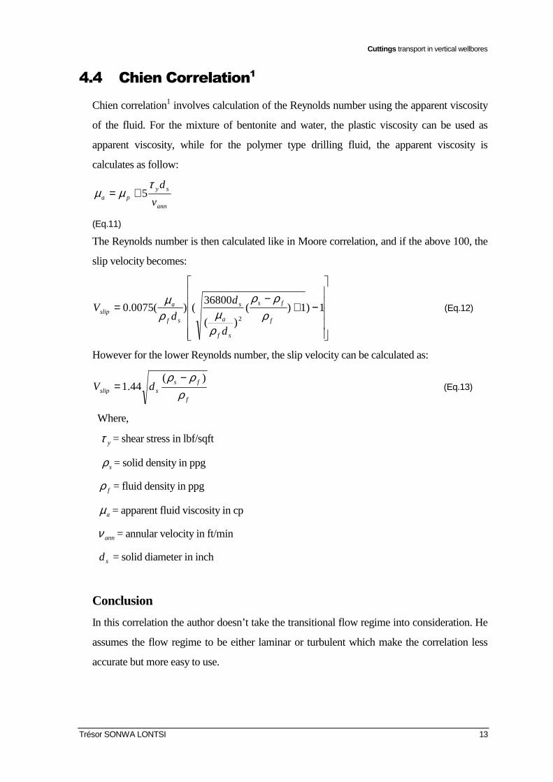
4.4 Chien Correlation1
Chien correlation1 involves calculation of the Reynolds number using the apparent viscosity
of the fluid. For the mixture of bentonite and water, the plastic viscosity can be used as
apparent viscosity, while for the polymer type drilling fluid, the apparent viscosity is
calculates as follow:
ann
sypa v
dτµµ 5+=
(Eq.11)
The Reynolds number is then calculated like in Moore correlation, and if the above 100, the
slip velocity becomes:
−+−
= 1)1)()(
36800()(0075.0
2 f
fs
sf
a
s
sf
aslip
d
d
dV
ρρρ
ρµρ
µ (Eq.12)
However for the lower Reynolds number, the slip velocity can be calculated as:
f
fssslip dV
ρρρ )(
44.1−
= (Eq.13)
Where,
yτ = shear stress in lbf/sqft
sρ = solid density in ppg
fρ = fluid density in ppg
aµ = apparent fluid viscosity in cp
annν = annular velocity in ft/min
sd = solid diameter in inch
Conclusion
In this correlation the author doesn’t take the transitional flow regime into consideration. He
assumes the flow regime to be either laminar or turbulent which make the correlation less
accurate but more easy to use.

Cuttings transport in vertical wellbores
Trésor SONWA LONTSI 14
4.5 Walker and Mayes correlation1
For Walker and Mayes, the apparent viscosity is determined by using an empirical relation
for shear stress due to particle slip. The corresponding equation for apparent viscosity is:
s
sa γ
τµ 479= (Eq.14)
Where,
sτ is the shear stress in lbf/sqft
sγ is the shear rate in 1/sec.
For particles Reynolds number bigger than 100, the slip velocity can be computed as:
f
fssslip dV
ρρρ )(
19.2−
= (Eq.15)
While for the lower Reynolds number, it is reduced to:
f
sssslip
dV
ργτ0203.0= (Eq.16)
Conclusion
As already mentioned in the Chien correlation, the flow regime is not taken into
consideration but also the wellbore geometry is not taking into account for the calculation of
the slip velocity. All this failed parameters make the correlation less accurate and less used.

Cuttings transport in deviated and horizontal wellbores
Trésor SONWA LONTSI 15
5 Cuttings transport in deviated and
horizontal wellbores
5.1 Literature Review
On the commissioning of various flow loops, a significant amount of experimental data was
collected on the effect of different parameters on cuttings transport under various conditions.
The observations made and subsequent analysis of the data collected provided the basis for
the work towards formulating correlations and models. Meanwhile, field experiences and
drilling data of inclined and horizontal wells provided practical operational guidelines and
the necessary basis for evaluation and improvement of the laboratory and theory based
models.
5.1.1 First experimental studies
Tomren et al (1986) performed a comprehensive study of steady state cutting transportation
in inclined wells by means of a flow loop. The study was conducted with a 5 inch and 40 feet
long transparent section. He investigated numerous angles of inclination, flow rates, drill
pipe rotations and pipe hole eccentricities. He identified visually the occurrence of cutting or
sliding beds based on various parameters. It was reported that the major factors that should
be considered in directional wells are fluid velocity, hole inclination, and mud and
rheological properties.
Okranjni and Azar (1986) studied specifically the effects of field measured mud
rheological properties like apparent viscosity, plastic viscosity, yield value and gel strength in
inclined wells. Since different muds could have the same rheological property, a ratio of
yield point (YP) to plastic viscosity (PV) was additionally used to distinguish the mud. The
study was done on the same flow loop as Tomren et al. (1986) using 15 different types of
mud systems including water. They noted that in the turbulent regime, the transport capacity
of mud was found to be independent of its rheological properties. The transport is affected
most by momentum forces which are mainly a function of mud density. Also in horizontal
wells, it was deduced that the turbulence would be a positive factor in the cleaning of the
annulus while the rotation of the drillpipe didn’t actually contribute to the cleaning of the

Cuttings transport in deviated and horizontal wellbores
Trésor SONWA LONTSI 16
bed, but it inhibited the formation of the bed. They lastly provided some field guidelines for
directional well drilling.
Sifferman and Becker (1992) performed experiments using an 8 inch 60 foot long flow
loop. They studied the effects of annular velocity, mud density, mud rheology, mud type,
cutting size, ROP, drill pipe rotary speed, drill pipe eccentricity, drill pipe diameter, and hole
angles (450 to 900 versus the vertical). The experiment was split into three phases to be able
to conduct a statistical analysis of the drilling parameters and validate the existence of
interactions between them. They found that cuttings size, mud weight have moderate
influence on the cuttings transport and showed that the transport ratio increases rapidly with
increase in annular mud flow rate then begins to level out or increase more slowly in the mud
flow rate range of 200 to 400 gpm.
Belavadi and Chukwu (1994) used an experimental flow loop with transparent acrylic
casing drill pipe annulus. Four different weights of bentonite mud samples 8.9 ppg,
9.3 ppg, 12 ppg, and 13 ppg with cutting chips of graded sizes small, medium and
large were introduced into the annular column from the bottom section of the
transparent acrylic pipe. The used a non-dimensional approach and observed that an
increase in the flow rate at higher fluid densities greatly increase the transport ratio
i.e. the ratio of the net cutting velocity and the average fluid annular velocity. This
effect is almost negligible when using low density fluids to transport large size
cuttings. They reported that the fluid density to viscosity ratio concept can be applied
to control drilling through sensitive formations. A small increase in the fluid density
to viscosity ratio results to a rapid decrease in the transport ratio. Similarly, a small
increase in the drag coefficient on the cuttings results to a large increase in the
transport ratio.
Kenny et al (1996) defined a lift factor that they used as an indicator of cuttings transport
performance. The lift factor is a combination of the fluid velocity in the lower part of the
annulus and the mud settling velocity. A flow loop of 8 in wellbore simulator, 100 ft long,
with a 4 in. drill pipe, was used in their study. The variables considered in this work were
drill pipe rotary speed, hole inclination, mud rheology, cuttings size, and mud flow rate.
Results have shown that the drill pipe rotation has an effect on hole cleaning in directional
well drilling. The level of enhancement in cuttings removal as a result of rotary speed is a
function of the combination of mud rheology, cuttings size, mud flow rate, and the manner in
Cuttings transport in deviated and horizontal wellbores
Trésor SONWA LONTSI 17
which the drill string behaves dynamically. They found out that, smaller cuttings are more
difficult to transport. However, with high rotary speed and high viscosity mud, small cuttings
become easier to transport. Low viscosity mud in the hole cleans better than high viscosity
mud with no pipe rotation.
Sanchez et al (1999), investigated the effect of drill pipe rotation on hole cleaning during
directional-well drilling. For his study, an 8 in. diameter wellbore simulator, 100 ft long, with
a 4 1/2 in. drill pipe was used. The variables considered in this experimental work were:
pipe rotation, hole inclination, mud rheology, cuttings size, and mud flow rate. Over 600
tests were conducted. The rotary speed was varied from 0 to 175 rpm. High viscosity and
low viscosity bentonite muds and polymer muds were used with 1/4 in. crushed limestone
and 1/10 in. river gravel cuttings. Four hole inclinations were considered: 40°, 65°, 80°, and
90° from vertical. His results show that drill pipe rotation has a significant effect on hole
cleaning during directional-well drilling if the pipe is freedom to spin around the hole axis.
This result is contrary to what has been published by previous researchers who forced the
drill pipe to rotate about its own axis. The level of enhancement due to pipe rotation is a
function of the simultaneous combination of mud rheology, cuttings size, and mud flow rate.
Also it was observed that the dynamic behaviour of the drillpipe plays a significant role in
the improvement of hole cleaning.
5.1.2 Theoretical studies
Gavignet and Sobey (1989) presented a two-layer cutting transport model on slurry
transport. They assumed that the cuttings had fallen to the lower part of the inclined
wellbore, and had formed a bed that slides up the annulus. Above this bed, a second layer
exists of pure mud. Eccentricity is taken into account in the geometrical calculations of
wetted perimeters and an apparent viscosity can be calculated for Non–Newtonian muds
using a rheogram written in polynomial form.
Sharma (1990) extended Gavignet and Sobey’s work modelling approach by separating the
particle into two separate layers. This allows having both a stationary and sliding bed at the
same time, and a bed sliding up inside the annulus on top and a bed sliding down at the
bottom.

Cuttings transport in deviated and horizontal wellbores
Trésor SONWA LONTSI 18
Martins and Santana (1992) presented a two layer model that is more versatile than
Gavignet and Sobey’s model because it allows particle to be in suspension in the upper layer.
The mean particle concentration in this layer is calculated form a concentration profile that
has been obtained from solving a diffusion equation.
Clark and Bickham (1994) developed a mechanistic model to describe hole cleaning.
Their model considers the various mechanisms involved in the transport of cuttings out of a
well i.e. rolling, lift and particle settling. Their publication concurs with industry opinion in
classifying flow rate as the most important factor in hole cleaning, and it considers fluid
density and rheology as the most important drilling fluid properties that affect hole cleaning.
The Herschel-Bulkley rheological model is also used, with the fluid yield stress being
dominant factor. But the influences of other rheological parameters like consistency index
and flow index are unclear.
Larsen et al (1997) developed a new mathematical model for estimating the minimum
fluid transport velocity for system with the inclination between 55° and 90°. They found that
the model worked fairly well within inclination 55° to 90°, and there were no correction
factors yet for the inclination less than 55°. From Larsen method it was known that there are
three parameters which affect the determination of minimum fluid annular velocity for
inclined hole: (1) inclination, (2) ROP and (3) mud density.
Kamp and Rivero (1999) developed a two-layered model for near horizontal wellbores. The
model consisted of a stationary or a moving bed below a layer of heterogeneous cuttings
suspension. They assumed that there was no significant slip velocity difference between the
particles and the mud. They took into account cuttings settling and re-suspension, but not the
vertical motion of the particles in the liquid. This simplified the model by assuming the
liquid and cuttings had the same density hence not taking into account the pressure and the
temperature effects. The model predicted thickness of the uniform bed as a function of mud
flow rate, cuttings diameter, mud viscosity, pipe eccentricity and other properties of the flow.
The results of the model were compared to a previous correlation based model. The closure
terms in the model were based on the experimental results. And Kamp et al.(1999)
suggested possible improvements to the model including solving separate momentum
equations for the solids and mud suspension layer.
Pilehvari et al (1999) carried out a review of cuttings transport in horizontal wells. The
advancement in cutting transportation research was summarized and suggestions were made
for much more work on turbulent flows of non-Newtonian fluids, effects of drill pipe

Cuttings transport in deviated and horizontal wellbores
Trésor SONWA LONTSI 19
rotation, comprehensive solid-liquid flow model and the development of a hole cleaning
monitoring system that receives all the available relevant data in real time for quick analysis
and determining the borehole status.
Hyun et al. (2000), formulated a mathematical three layer model to predict and interpret the
cuttings transport in deviated wellbore from vertical to horizontal. The model considered the
following layers: (1) a stationary bed of cuttings in low side of the borehole, (2) moving bed
layer above the stationary one, (3) a heterogeneous suspension layer at the top. They
modelled three segments to deal with the well deviation: horizontal segment from 60° to 90°,
transient segment from 30° to 60°, and a vertical segment from 0 to 30°. For every segment
they set up continuity equations and momentum equations. They analyzed the interface
interaction using the correlations. They reported effects of annular velocity, fluid rheology,
and angle of inclination on cuttings transport. The model predictions based on the simulation
are in good agreement with the experimental data published by other.
5.2 Factors influencing the cuttings transport
They are several factors that affect the transport of the cuttings while drilling deviated wells.
Cuttings transport is affected by several interrelated mud, cuttings and drilling parameters, as
shown in the table below. For the hole cleaning, annular and mud viscosity are generally
considered to be the most important parameters.
Well profile and geometry • Hole inclination angle and doglegs
• Casing/hole and drill pipe diameters
• Drillstring eccentricity
Cuttings and cuttings bed
characteristics
• Specific gravity
• Particle size and shape
• Reactivity with mud
• Mud properties
Flow characteristics
• Annular velocity
• Annular velocity profile
• Flow regime

Cuttings transport in deviated and horizontal wellbores
Trésor SONWA LONTSI 20
Mud properties • Mud weight
• Viscosity, especially at low shear rates
• Gel strengths
• Inhibitiveness
Drilling parameters • Bit type
• Penetration rate
• Differential pressure
• Pipe rotation
Table 1: Drilling parameters influencing the cuttings removal
5.2.1 Annular velocity
In case of an inclined annulus, the axial component of particle slip velocity play a less
important role, and one could conclude that to have satisfactory transport, the annular mud
velocity in this case may be lower than in the vertical annulus. This however is a misleading
conclusion. The increasing radial component of the particle slip velocity pushes the particle
toward the lower wall of the annulus, causing a cuttings bed to form as already mentioned.
Consequently, the annular mud velocity has to be sufficient to avoid the bed formation. It is
expected that an increase in flow rate will always cause more efficient removal of the drilled
cuttings out of the annular space. However, an upper limit of the flow rate is dictated by:
Rig hydraulic power
Equivalent Circulation Density
Susceptibility of the open hole section to hydraulic erosion
5.2.2 Wellbore Inclination angle
It has been well established from previous laboratories work that as hole angle increases
from zero to about 65 degrees from vertical, hole cleaning becomes more difficult and
hydraulic requirements increase, likewise. The flow rate requirements peak around hole
angles between 65°-75° (degrees) from vertical and slightly decrease toward the horizontal.
Also, it has been shown that at angles between 30°-60° (degrees) from vertical, a sudden
pump shut-down causes sloughing of accumulated cuttings bed to bottom and may cause a
serious problem of pipe sticking. Although, hole inclination causes difficulties in hole
cleaning, its choice is mandated by the anticipated geological conditions and by field

Cuttings transport in deviated and horizontal wellbores
Trésor SONWA LONTSI 21
development company objectives. Reservoir inaccessibility, offshore drilling, avoiding
troublesome formations, and horizontal drilling into the reservoir are some of the geological
conditions that dictate hole angle. Company objectives in the total development of a field,
such as primary production objectives, secondary production objectives, economic
objectives, environmental objectives, etc., are also governing factors in hole angle selection.
But in order to reduce the inclination effect the planning of the wellbore trajectory must be as
straight as possible.
5.2.3 Mud Properties
The functions of the drilling mud are many and have competing influences. These include
• cleaning the bottom hole and annulus
• wellbore stabilization (mechanical and chemical)
• cooling and lubrication of the drill string
• formation evaluation
• Prevention of formation intrusion into the wellbore during conventional drilling
(i.e., over-balanced).
Generally speaking, different drilling fluid types provide similar cuttings transport if their
downhole properties also are similar. However, selection of optimum properties requires
careful consideration of all related parameters. Clearly, mud properties must be maintained
within certain limits to be effective without being destructive or counter-productive.
Properties of particular interest to hole cleaning include mud weight, viscosity, gel strengths
and level of inhibition.
1). Mud weight helps buoy cuttings and slow their settling rate1 (as shown by Stokes’
law in the first chapter), but it is really not used to improve hole cleaning. Instead, mud
weights should be adjusted based only on pore pressure, fracture gradient and wellbore-
stability requirements. Vertical wells drilled with heavy muds normally have adequate
hole cleaning as compared to highly deviated directional wells drilled with low-density
fluids.
Wellbore instability is a special case where mud weight clearly targets the cause, rather
than the symptoms, of hole-cleaning problems. As a rule, formations drilled directionally
require higher mud weights to prevent bore-hole failure and sloughing into the annulus.
What can appear as a hole-cleaning problem at the surface, in fact, can be a stress-related

Cuttings transport in deviated and horizontal wellbores
Trésor SONWA LONTSI 22
problem which should be corrected by increasing the mud weight? Alternative actions to
improve cuttings transport may help but will not eliminate the basic problem.
2). Mud viscosity helps determine carrying capacity1. For vertical wells, yield point
historically has been used as the key parameter which was thought to affect hole cleaning.
More recently, evidence concludes that Fann 6- and 3-RPM (Rotation per Minute) values are
better indicators of carrying capacity (even in vertical wells). These values are more
representative of the LSRV (Low-Shear Rate Viscosity)4 which affects hole cleaning in
marginal situations. Coincidentally, most viscosifiers (clays, for example) added to increase
yield point also increase 6- and 3-RPM values. One common rule of thumb is to maintain the
3-RPM value so that it is greater than the hole size (expressed in inches) in high-angle wells.
The Low-Shear Yield Point (LSYP)4, calculated from 6- and 3-RPM values, has also gained broad acceptance for quantifying LSRV:
LSYP = ( ) rpmrpm 632 θθ −× (Eq.17)
LSYP can play an even more important hole-cleaning role in directional wells, if it is applied
in accordance with the specific well conditions. For example, in laminar flow, there is a
clear correlation between improved hole-cleaning performance and elevated LSYP,
especially in conjunction with the rotation of eccentric pipe. On the other hand, low LSYP
values are preferred for turbulent-flow hole cleaning, because turbulence could be achieved
at lower flow rates. Elevated LSRVs make it possible to achieve superb hole cleaning at
much lower flow rates than conventional systems.
3).Gel strengths provide suspension under both static and low-shear-rate conditions.
Although closely related to viscosity, gel strengths sometimes are overlooked with regard to
their effects on hole cleaning. Quickly developing gels which are easily broken can be of sig-
nificant help. Excessively high and/or progressive gels, on the other hand, should be avoided
because they can cause or exacerbate a number of serious drilling problems.
5.2.4 Drill String Rotation
It has been demonstrated in laboratory studies and reported in field cases, that drill string
rotation with the induced modes of vibrations (torsional, longitudinal, and lateral) has
moderate to significant effects on hole cleaning in directional wells. The level of
enhancement in drilled cuttings removal due to drill string rotation is a function of the
combination of mud rheology, cuttings size, flow rate, and the dynamic behavior of the

Cuttings transport in deviated and horizontal wellbores
Trésor SONWA LONTSI 23
string. It is believed that the whirling motion of the string as it rotates is the major
contributor to the cleaning process. Mechanical agitation of the cuttings bed and its
exposure to higher fluid velocities are the beneficiaries of this motion.
Although there is a definite gain in hole cleaning due to drill pipe rotation, it must be
recognized also that there are limitations that may have to be imposed as well. For
example, pipe rotation cannot be activated during the sliding mode while building hole
angle. Also, pipe rotation induces cyclic stresses that can accelerate pipe failure due to
fatigue, causes excessive casing wear and in some cases mechanical destruction of the
walls of open hole sections. Additionally, in slim-hole drilling (hole diameter less than
6"), high pipe rotation may cause an increase in the annular friction pressure losses and
therefore and increasing in ECD. Also very important to highlighted that all the changes
of such parameters as RPM must be done according to the capacity of the tools used like,
motor, RSS, MWD and LWD tools.
Figure 2: Lifting of the cuttings due to pipe rotation10
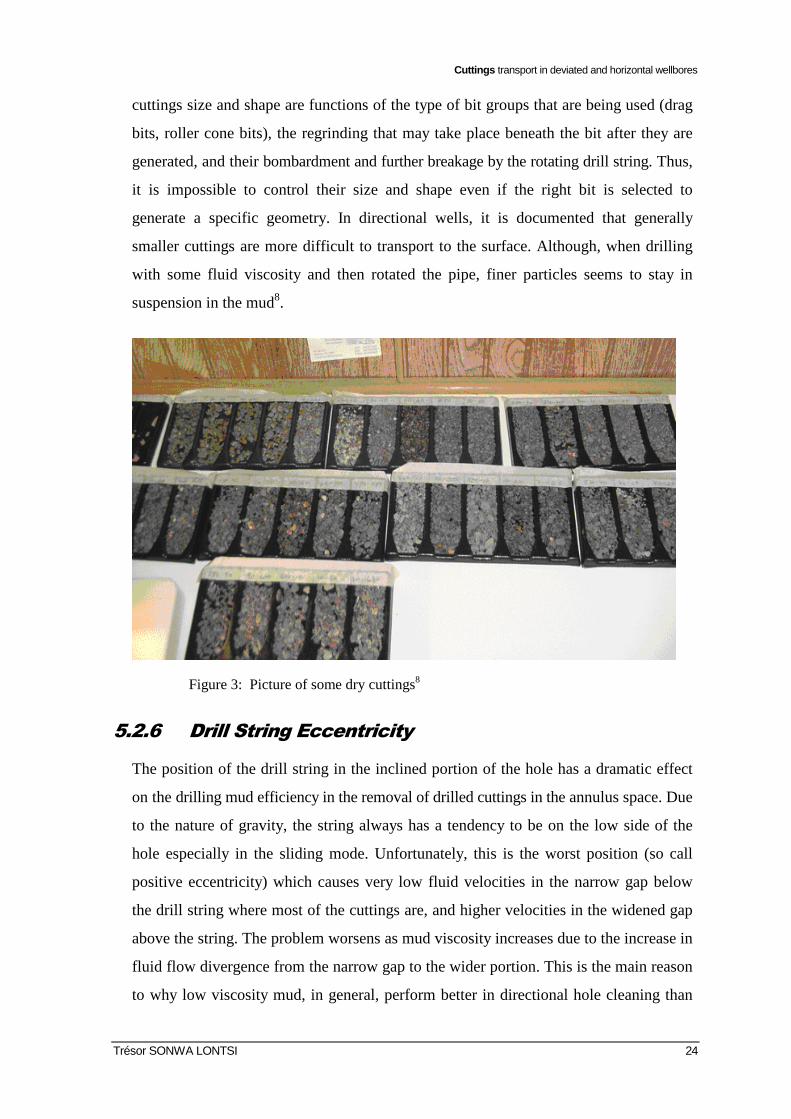
5.2.5 Drilled Cuttings Properties
The size, the shape, and the specific gravity of drilled cuttings are what affect their
dynamic behavior in a flowing media. The specific gravity of most rocks that are drilled
is on the average of about 2.6 and therefore, can be assumed to be known. However, the
Cuttings transport in deviated and horizontal wellbores
Trésor SONWA LONTSI 24
cuttings size and shape are functions of the type of bit groups that are being used (drag
bits, roller cone bits), the regrinding that may take place beneath the bit after they are
generated, and their bombardment and further breakage by the rotating drill string. Thus,
it is impossible to control their size and shape even if the right bit is selected to
generate a specific geometry. In directional wells, it is documented that generally
smaller cuttings are more difficult to transport to the surface. Although, when drilling
with some fluid viscosity and then rotated the pipe, finer particles seems to stay in
suspension in the mud8.
Figure 3: Picture of some dry cuttings8
5.2.6 Drill String Eccentricity
The position of the drill string in the inclined portion of the hole has a dramatic effect
on the drilling mud efficiency in the removal of drilled cuttings in the annulus space. Due
to the nature of gravity, the string always has a tendency to be on the low side of the
hole especially in the sliding mode. Unfortunately, this is the worst position (so call
positive eccentricity) which causes very low fluid velocities in the narrow gap below
the drill string where most of the cuttings are, and higher velocities in the widened gap
above the string. The problem worsens as mud viscosity increases due to the increase in
fluid flow divergence from the narrow gap to the wider portion. This is the main reason
to why low viscosity mud, in general, perform better in directional hole cleaning than

Cuttings transport in deviated and horizontal wellbores
Trésor SONWA LONTSI 25
high viscosity mud. Since eccentricity is governed by the pre-selected wellbore
trajectory and the dynamic behavior of the drill string, its adverse impact on hole
cleaning is unavoidable.
Figure 4: Comparison between concentric (left) and eccentric (right) drill pipe annular flow distribution8
5.2.7 Rate of Penetration
Under equal conditions, an increase in ROP causes an increase in the drilled cuttings
concentration in the annulus. Therefore, to maintain an acceptable and effective hole
cleaning, other controllable variables such as hydraulics and rotary speed must be
adjusted. If the limits of these variables have been reached then the only alternative is to
decrease the rate of penetration. Although, a decrease in ROP will have a negative
impact on well cost, the benefits of avoiding drilling problems such as pipe sticking
and excessive torque and drag can outweigh the losses.
5.3 Hole cleaning and cuttings bed formation
Based on laboratory researches and on field experiences, deviated and horizontal wellbores
lead to some of the most troublesome hole cleaning problem. Removing cuttings from the
deviated part of the wellbore trajectory (see Figure 5) is a big challenge and will be discussed
in details in this chapter.

Cuttings transport in deviated and horizontal wellbores
Trésor SONWA LONTSI 26
5.3.1 Cuttings bed formation
This graph gives a general idea of where the cuttings start to accumulate in the inclined wellbore trajectory.
Figure 5: Well trajectory in directional drilling
During the drilling of the deviated part of the hole, the directional driller must slide for
changes in direction and/or inclination, and rotate to drill the hold part. The sliding is the
worst operation because the drill pipe lies against the low side of the hole which increases
hole cleaning problem. The flow of the cuttings in the annulus is a dynamic process and is
subject to many forces that were already mentioned in the previous chapter for the vertical
section. The forces and the velocity components acting on a cutting are shown in the figure
below in the figure 6 and 7.
Cuttings transport in deviated and horizontal wellbores
Trésor SONWA LONTSI 27
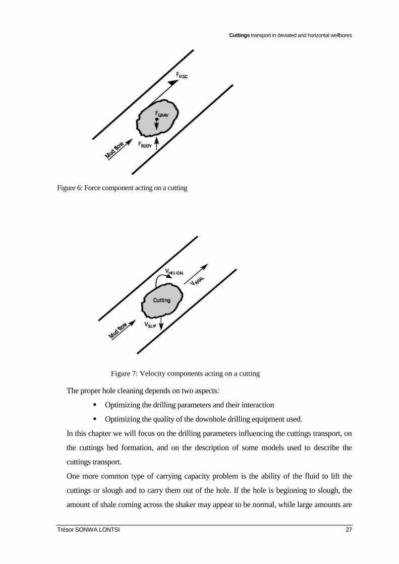
Figure 6: Force component acting on a cutting
Figure 7: Velocity components acting on a cutting
The proper hole cleaning depends on two aspects:
Optimizing the drilling parameters and their interaction
Optimizing the quality of the downhole drilling equipment used.
In this chapter we will focus on the drilling parameters influencing the cuttings transport, on
the cuttings bed formation, and on the description of some models used to describe the
cuttings transport.
One more common type of carrying capacity problem is the ability of the fluid to lift the
cuttings or slough and to carry them out of the hole. If the hole is beginning to slough, the
amount of shale coming across the shaker may appear to be normal, while large amounts are

Cuttings transport in deviated and horizontal wellbores
Trésor SONWA LONTSI 28
being collecting in the hole. Sometimes the appearance of the cuttings will indicate poor hole
cleaning. If the cuttings are rounded, it may indicate that they have spent an undue amount of
time in the hole. The condition of the hole is usually one of the best indicators of the hole
cleaning difficulty. Fill on bottom after a trip is an indicator of inadequate hole cleaning.
However, the absence of the fill doesn’t mean that there is not a cleaning problem. Large
amounts of cuttings may be accumulating in washed out places zones in the borehole. Drag
while pulling the drill string to make a connection may also indicate inadequate cleaning.
When the pipe is moved upward, the swab effect may be sufficient to dislodge cuttings
packed into a washed-out section of the hole. The sudden dumping of even a small amount a
material is often enough to cause severe drag or sticking.
The ability of the fluid to lift a piece of rock is affected first by the difference of density of
the rock and the fluid. If there is no difference in densities, the rock will be suspended in the
fluid and will move on a flow stream at the same velocity as the fluid. As the density of the
fluid is decreased, the weight of the rock in the fluid is increased and it will tend to settle.
The shear stress of the fluid moving by the surface of the rock will tend to drag the rock with
the fluid. The velocity of the rock will be somewhat less than the velocity of the fluid. As
already mentioned before, the difference in velocities is usually referred to as slip velocity.
The shear stress that is supplying the drag force is a function of shear rate of the fluid at the
surface of the rock and the viscosity of the mud at this shear rate. A number of others factors
as wall effects, inter-particle interference, pipe eccentricity, hole angle and the turbulent flow
around the particles make exact calculations of the slip velocity impossible.
When drilling in an inclined annulus at an angle θ from the vertical, there will be two
components for the slip velocity:
θcos. slipaslip VV = (Eq.18)
θsin. sliptslip VV = (Eq.19)
Where, aslipV . , tslipV . are the axial and radial components of the average slip velocity,
respectively as shown in the Figure 8 below.

Cuttings transport in deviated and horizontal wellbores
Trésor SONWA LONTSI 29
aslipV . =Vs aslipV . = θcossV tslipV . =Vs
tslipV . =Vs tslipV . = θsinsV aslipV . =0
Figure 8: Particle settling velocity in an inclined annulus from TOMREN14
When the angle of inclination is increased, the axial component of the slip velocity
decreases, reaching zero value at the horizontal position of the annulus. When these
conditions are taken into account, all factors that may lead to improved cuttings transport by
a reduction of the particle slip velocity will have a diminishing effect while angle of
inclination is increasing. When reaching the hole section with an inclination between 30 and
60 degrees, the cuttings accumulation in the annulus adds a further problem to the drilling
process. An equilibrium between cuttings bed erosion and cuttings settling at the low side of
the hole results in a “stable” cuttings bed until the mud circulation is interrupted e.g. when
making a connection. As soon as the dragging forces of the flowing mud discontinue,
cuttings beds may slide down the low side of the hole like an avalanche leading to
mechanical sticking at the lower portion of the drill string (see Figure 9).
Cuttings accumulations can be diff icult to erode or re-suspend, so mud properties and
drilling practices which minimize their formation should be emphasized. Clearly, cuttings
which remain in the flow stream do not become part of a bed or accumulation. Mud
suspension properties are important, especially at low flow rates and under static
conditions. Cuttings beds, such as those formed in directional wells, can take on a wide
range of characteristics that impact hole-cleaning performance. For example, clean sand
drilled with clear brine will form unconsolidated beds which tend to roll rather than slide
Cuttings transport in deviated and horizontal wellbores
Trésor SONWA LONTSI 30
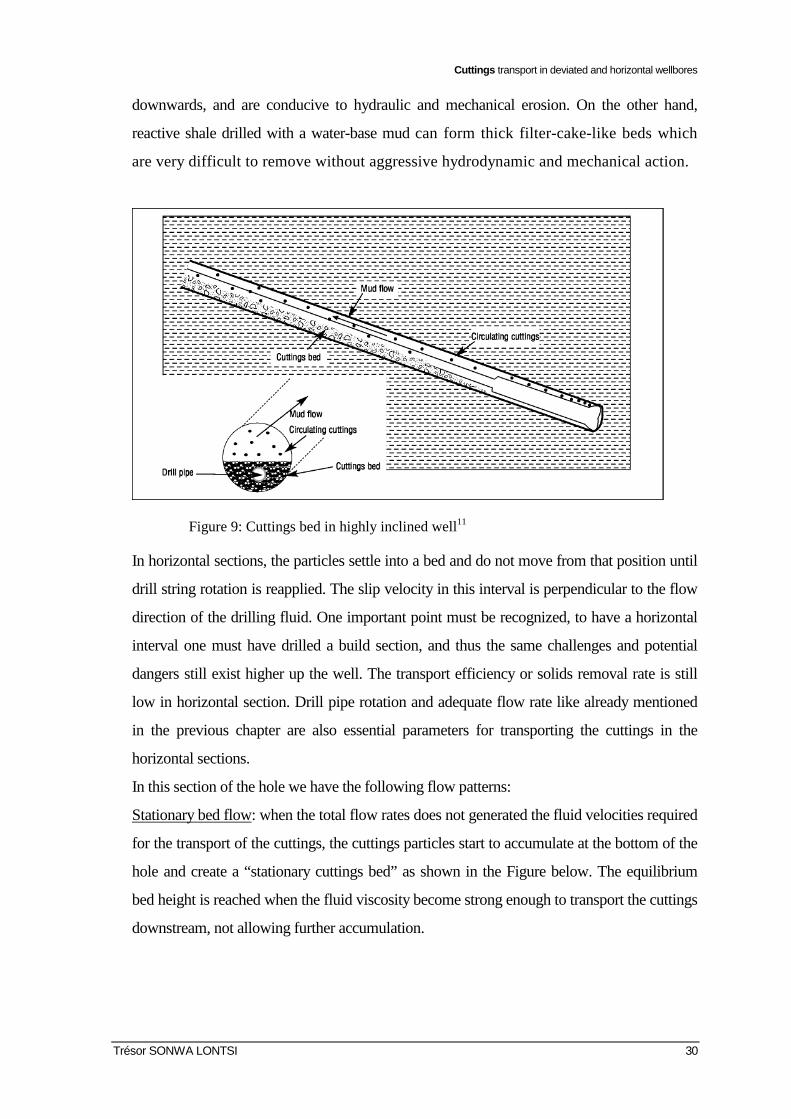
downwards, and are conducive to hydraulic and mechanical erosion. On the other hand,
reactive shale drilled with a water-base mud can form thick filter-cake-like beds which
are very difficult to remove without aggressive hydrodynamic and mechanical action.
Figure 9: Cuttings bed in highly inclined well11
In horizontal sections, the particles settle into a bed and do not move from that position until
drill string rotation is reapplied. The slip velocity in this interval is perpendicular to the flow
direction of the drilling fluid. One important point must be recognized, to have a horizontal
interval one must have drilled a build section, and thus the same challenges and potential
dangers still exist higher up the well. The transport efficiency or solids removal rate is still
low in horizontal section. Drill pipe rotation and adequate flow rate like already mentioned
in the previous chapter are also essential parameters for transporting the cuttings in the
horizontal sections.
In this section of the hole we have the following flow patterns:
Stationary bed flow: when the total flow rates does not generated the fluid velocities required
for the transport of the cuttings, the cuttings particles start to accumulate at the bottom of the
hole and create a “stationary cuttings bed” as shown in the Figure below. The equilibrium
bed height is reached when the fluid viscosity become strong enough to transport the cuttings
downstream, not allowing further accumulation.

Cuttings transport in deviated and horizontal wellbores
Trésor SONWA LONTSI 31
Figure 10: Stationary cuttings bed
Moving bed flow: When increasing the volumetric flow rates, there is a point which the
cuttings break into a slowly moving cuttings bed as shown in the Figure below.
Figure 11: Moving cuttings bed
Dispersed bed flow: The dispersed bed flow normally occurs when the total volumetric flow
rate high enough to suspend all the solids particles in the liquid as you can see in the figure
below.
Figure 12: Dispersed cuttings bed
Although particles cannot avalanche in the horizontal sections, pack-offs can still be induced
if the drill pipe is moved axially in the interval with a cuttings bed present. Hole cleaning
should be perform prior to tripping out of the hole so that the drill string isn’t dragged
through a cuttings bed or the cuttings are not pushed up into the build section where
avalanching can occur. Drill pipe pulled through a cuttings bed will act like a “bulldozer”,
accumulating cuttings across tool joints, the BHA or at the bit.
The Figure 13 below illustrated the pack-off effect that appears when tripping out of the hole
in the horizontal section:
Figure 13: Pack-off while pulling the BHA out of the hole
Cuttings transport in deviated and horizontal wellbores
Trésor SONWA LONTSI 32
5.3.2 Hole cleaning during the drilling operations
Hole cleaning problems start when the employed operating parameters fail to efficiently
circulate cuttings to surface. Experience has shown that this can occur whether with
rotary drilling or drilling with motors is employed. The problems have further been
identified in both the drilling phase and the tripping phase.
These two modes represent two different configurations of cuttings bed build up processes
and hole cleaning practices in the wellbore.
Drilling phase
During the drilling phase, there is an equilibrium cuttings bed height that can be
used as an indication of the efficiency of the hole cleaning by measuring the amount
of cuttings at surface versus the calculated volume of cuttings expected to be
generated when drilling out the formation During this mode even though the bed reaches
a steady state (provided parameters remain unchanged) the cuttings bed height is not
necessarily regularly distributed along the drill string. For example, the section
directly above the BHA encounters high volumes of cuttings as the smaller annular
clearance in the BHA generates high mud velocity and therefore avoids cuttings
accumulation but this effect is greatly reduced in the drill pipe section resulting in the
immediate settling of the cuttings into beds or dunes.
For this mode then, the hole cleaning performance corresponds directly to the final
equilibrium bed height (provided parameters remain unchanged).
Tripping phase
During tripping phase, cuttings can build-up under several conditions:
Natural sedimentation of solid particles when mud flow stops
Dragging of the drill string through the existing cuttings bed creates
localized “dunes” of cuttings
Avalanching of the cuttings when the bed is established in the critical angle
section (30 - 60 degrees) of the well
For this mode, the hole cleaning performance is related to the speed at which the system
decays the cuttings and to the final cuttings bed height

Cuttings transport in deviated and horizontal wellbores
Trésor SONWA LONTSI 33
5.4 Some methods to determine the bed thickness
Two methods are presented in this thesis to highlight the determination of the cuttings
bed thickness in the wellbore. The first method is the empirical correlations and the
second one is the method of Artificial Neural Networks developed by Ozbayoglu et al
(2002). In order to develop a more general empirical correlation, which will be valid
for a wide range of conditions, it is essential to describe the variables in dimensionless
form. Thus a dimensional analysis is conducted. It is generally believed that the height
of a cuttings bed is the essential information for controlling hole cleaning
performance and a successful drilling operation6,12. Major independent drilling
variables, which control the development of a cuttings bed in a wellbore, considered
in these methods are inclination angle, feed cuttings concentration, fluid density, a
term representing the apparent fluid viscosity, average velocity and dimensions of the
pipe and wellbore.
A dimensional analysis is conducted by using those independent variables in order to
develop dimensionless groups that can be correlated for estimating bed height. After
applying the Buckingham - π Theorem which is a key theorem in dimensional
analysis, five dimensionless groups are developed and defined as:
1π = cC = volume of cuttings/volume of annulus
2π =α (Eq.20)
w
bed
A
A=3π (Eq.21)
Re4 NvD ==µ
ρπ (Eq.22)
Re25
1
Nv
gD ==π (Eq.23)
5.4.1 Empirical correlation using Least Square Method
The relation between the dimensionless bed area and the rest of the dimensionless
groups can be written as:
),,,( Re Frcw
bed NNCfA
A α= (Eq.24)
Where:

Cuttings transport in deviated and horizontal wellbores
Trésor SONWA LONTSI 34
bedA Cross-section flow area of the cutting bed in sqft
wA Cross-section flow area of the wellbore in sqft
cC Feed cuttings concentration
α Angle in degree versus vertical
ReN Reynolds number
FrN Froude number
The relation between each dimensionless group and the dimensionless bed area is
presented in the Figure 1416.
Figure 14: Change of each dimensionless group with the dimensionless cuttings bed area
Flow loop experiments with a simulated drill-string have shown that the inclinations
up to 65° degrees do not affect the bed height. Thus, inclination angleα is removed
from the equation above. From the analysis (see Figure 14), it is observed that a
possible relationship among these dimensionless group is the multiplication form.
Thus, a general representation of the dimensionless bed area is expressed as:
432 )()()( Re1k
Frkk
cw
bed NNCkA
A= (Eq.25)
In order to determine the coefficient,1k experimental data collected at the Tulsa
University flow loop are used. Information established from the cuttings experiments
with different muds was analyzed. A set of empirical correlations was developed
using multivariate regression (StatisticaTM). The least square method is used during
this analysis.

Cuttings transport in deviated and horizontal wellbores
Trésor SONWA LONTSI 35
The following equations are obtained:
For 9.0≥N
2164.02198.0Re
0035.0 )()()(1232.4 −−= FrCw
bed NNCA
A (Eq.26)
For 9.06.0 << N
0681.00374.0Re
0697.0 )()()(7115.0 −−= FrCw
bed NNCA
A (Eq.27)
For 6.0≤N
0646.01502.0Re
0024.0 )()()(0484.1 −−= FrCw
bed NNCA
A (Eq.28)
The correlation coefficients (R2 = estimated variation/ total variation) for these
equations are 0.8612, 0.9318 and 0.7966 respectively with the perfect match if R2 = 1.
The result of the experimental results and the empirical correlation is compared in the
graph (Figure 15) below, which shows is less accuracy at N > 0,9 .
Figure 15: Experimental results versus empirical correlation results16
5.4.2 Artificial Neural Network (ANN) 16
Another method used to estimates the cuttings bed height is using the ANN. The
popularity of ANN is increasing due to its wide range of possible applications, and its
capability of handling the nonlinearities that cannot be described by conventional
mathematical functions16.A neural network has a parallel distributed architecture with

Cuttings transport in deviated and horizontal wellbores
Trésor SONWA LONTSI 36
a large number of nodes and connections16.Connection points are connected from one
node to another and are associated with a weight. A simple view of the network
structure and behaviour is given in Figure 16.
Figure 16: Schematic view of a basic Neural Network System
Network layers
The input layer: the nodes in this layer are called input units, which encode the
instance presented to the network for processing. For example, each input unit may be
designated by an attribute value possessed by the instance. In this study, the inputs are
feed cuttings concentration, Reynolds Number and Froude Number; thus, there are
three input nodes.
The hidden layer: The nodes in this layer are called hidden units, which are not
directly observable and hence hidden. They provide nonlinearities for the network. In
this study, a single hidden layer is used with ten hidden nodes. The number of hidden
layers and nodes are determined by trial and error.
The output layer: the nodes in this layer are called output units, which encode possible
concepts or values to be assigned to the instance under consideration. Here, the only
output is the cuttings bed area; thus, there is only one output node.
Backpropagation
The backpropagation network is a technique that is probably the most well known and
widely used among the current types of neural network systems available16. A
backpropagation network is a multi-layer feed forward network with a different

Cuttings transport in deviated and horizontal wellbores
Trésor SONWA LONTSI 37
transfer function in the artificial neuron and more powerful learning rule. The learning
rule is known as backpropagation, which is a kind of gradient descent technique with
backward error propagation. The training instance set for the network must be
presented many times in order for the interconnection weights between the neurons to
settle into a state for correct classification on input patterns. While the network can
recognize patterns similar to those they have learned they do not have the ability to
recognize new patterns. This is true for all supervised learning networks. In order to
recognize new patterns, the network needs to be retrained with these patterns along
with previously known patterns. If only new patterns are provided for retraining, then
old patterns may be forgotten. In this way, learning is not incremental over time. This
is a major limitation for supervised learning of networks.
Reynolds number, Froude number, feed concentration are used as inputs for training
the network. The network determines dimensionless bed area using the weight
functions obtained during training.
Comparison done by Ozbayoglu et al (2002) between both methods describe shown
that ANN estimates the cuttings bed thickness more accurately than the empirical
methods at lower bed thickness. As it is shown in the Figure 17 below the ANN
estimation follow the perfect match from zero to the high value of the ration between
the bed area and the total wellbore area.
Figure 17: Experimental results versus ANN results16

Cuttings transport in deviated and horizontal wellbores
Trésor SONWA LONTSI 38
5.5 Critical angle in deviated wellbores
Range Angle in degrees
Near-vertical I
0-10
Low II
10-30
Intermediate III
30-60
High IV
60-90
Table 2: range based on hole angle
Their keys of consequences are listed here according to angle range:
Near-vertical and low ranges: cuttings concentrations are little and there is not
cuttings bed formation.
Intermediate range: cuttings concentration, bed thickness and property for slumping.
High range: bed thickness and physical characteristics.
The limits of each range should be considered only as guidelines, since all are affected by
bed stability, borehole roughness, cuttings characteristics and drilling fluid properties, among
others. Figure 8 illustrates relative hole-cleaning difficulty based on angle. In vertical
and near-vertical wells, cuttings beds do not form, but failure to properly transport and
suspend cuttings can cause fill on bottom or bridging in doglegs. In directional wells, the
build section in the intermediate range typically is the most difficult to clean, because
cuttings beds can slide or “slump” opposite the direction of flow. Boycott settling which is
explaining on the next page can exacerbate the problem. Sliding tendencies start dissipating
at angles greater than about 60°, due to the corresponding decrease in the gravitational force
vector.

Cuttings transport in deviated and horizontal wellbores
Trésor SONWA LONTSI 39
Figure 18: Hole cleaning difficulty versus inclination8
All four ranges may co-exist in the same directional well. For most cases, fluid properties
and drilling practices should strive to minimize problems in the most critical interval.
Hole-cleaning factors considered optimum for one interval may be inadequate in another.
For example, requirements differ for large-diameter casing (which severely limits annular
velocity), the build interval (which promotes cuttings-bed formation and sliding) and the
production formation drilled horizontally (which may be shear sensitive and tend to wash
out).
Boycott settling8, an accelerated settling pattern which can occur in inclined wellbores, is
named after the physician who first reported that particles in inclined test tubes settle 3 to 5
times faster than in vertical ones. Boycott settling is the consequence of rapid settling
adjacent to the high (top) and low (bottom) sides of inclined well-bores. This causes a
pressure imbalance which drives the lighter, upper fluid upwards and any cuttings beds on
the low side downwards. Angles from 40 to 60° are particularly troublesome. At rela-
tively low flow rates, mud flows mainly along the high side and accelerate or enhance the
Boycott effect. High flow rates and pipe rotation can disrupt the pattern and improve hole
cleaning.

Cuttings transport in deviated and horizontal wellbores
Trésor SONWA LONTSI 40
Figure 19: Illustration of the Boycott Settling Effects in the range of 40 to 60° inclination8
5.6 Modes of Cuttings Transport in horizontal
section
Based on visual observations of the laboratory experiments done in the past work, the
transport process can be categorize while assuming a perfect concentricity of the pipe into
the following flow patterns as shown in the Figure 20 below :
Figure 20: Schematic representation of different modes of transport13

Cuttings transport in deviated and horizontal wellbores
Trésor SONWA LONTSI 41
At high flow velocity, mobile particles on the uppermost layer of the bend tend to glide
forward on the top of a stationary bed forming a dilated dispersed layer; thus, we have a
three-layer-flow pattern: a stationary bed of particles of uniform concentration, a dispersed
layer in which particle concentration is varied, and an essentially clear fluid flow region on
top as shown in the Figure 20(b). As the flow velocity is increased, the intensity of turbulent
eddies grows in strength and eventually reaches a stage at which these turbulent eddies are
strong enough to lift the topmost particles of the dispersed layer into the fluid flow region
and carry them in a turbulent suspension mode. At this stage, we also have a three layer flow
pattern but with a slightly different composition than that shown in Figure 20(b). The figure
20(c) shows a heterogeneous suspension layer on the top of a dispersed layer and a uniform
concentration bed that can either be stationary or moving in a king of “bloc”21. As more and
more particles are picked up by turbulent eddies as the flow velocity further increases, the
bed will get thinner and eventually the bed will disappear, leaving behind a dispersed layer
and a heterogeneous suspension layer. This flow pattern is hereafter referred as two layer
flow pattern as we can see in the Figure 20(d). Finally, with further increases in the annular
flow velocity, all particles will be transported in the heterogeneous or homogeneous
turbulent suspension mode. This flow pattern is hereafter referred as a single layer flow
pattern as illustrated in the Figure 20(e).
5.6.1 Wellbore geometry in horizontal interval
In order to solve the equations for the determination of the bed height in the borehole, the
area and contact surfaces for each layer are required. All possible wellbore configurations
can be categorized into six major cases as shown in the Figure 21. For each layer case, the
area, contact surfaces, etc can be determined by using basic trigonometry and geometry
equations. The cases 4-6 can normally not happen in the horizontal section because we
assume that the pipe will be almost every time at the low side of the borehole wall. The
symbol “e” in the graph below represents the eccentricity. Eccentricity can be positive if “e”
bigger than zero or negative if “e" smaller than zero.
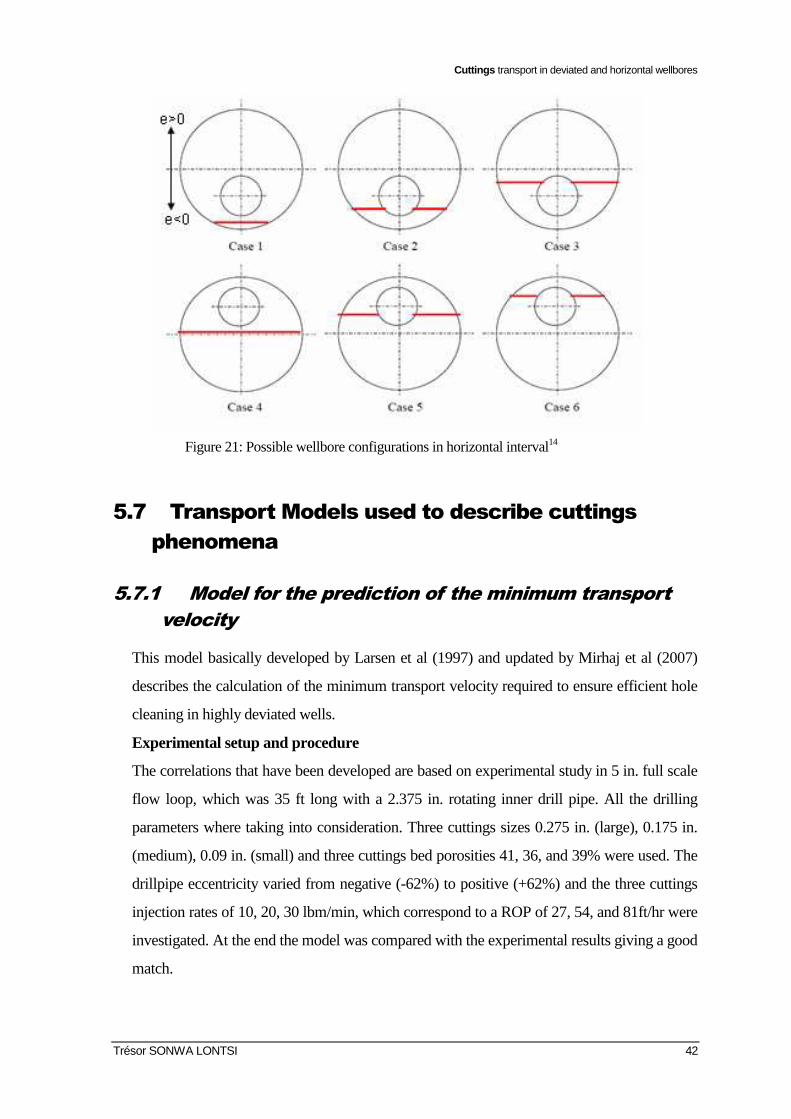
Cuttings transport in deviated and horizontal wellbores
Trésor SONWA LONTSI 42
Figure 21: Possible wellbore configurations in horizontal interval14
5.7 Transport Models used to describe cuttings
phenomena
5.7.1 Model for the prediction of the minimum transport
velocity
This model basically developed by Larsen et al (1997) and updated by Mirhaj et al (2007)
describes the calculation of the minimum transport velocity required to ensure efficient hole
cleaning in highly deviated wells.
Experimental setup and procedure
The correlations that have been developed are based on experimental study in 5 in. full scale
flow loop, which was 35 ft long with a 2.375 in. rotating inner drill pipe. All the drilling
parameters where taking into consideration. Three cuttings sizes 0.275 in. (large), 0.175 in.
(medium), 0.09 in. (small) and three cuttings bed porosities 41, 36, and 39% were used. The
drillpipe eccentricity varied from negative (-62%) to positive (+62%) and the three cuttings
injection rates of 10, 20, 30 lbm/min, which correspond to a ROP of 27, 54, and 81ft/hr were
investigated. At the end the model was compared with the experimental results giving a good
match.

Cuttings transport in deviated and horizontal wellbores
Trésor SONWA LONTSI 43
Cuttings velocity5
A simple mass balance is assume, where,
Mass of cuttings generated at the bit is equal the mass of cuttings transported to the surface.
cutconcholecutinjcut CAVq ρρ .... = (Eq.29)
From this equation, we can derive the cutting velocity ( cutV ) as a function of the ROP.
conchole
pipe
cut
CA
A
ROPV
×
−
=
361
2 (Eq.30)
And the same equation can be calculated by inserting in the equation 25 by the pipe and hole
diameter. So, the new equation5 will be:
conchole
pipe
cut
CD
D
ROPV
×
−
=
361
2 (Eq.31)
Based on the regression analysis a relation was fund to calculate the cuttings generated as a
function of the ROP5. Figure 10 can be expressed in terms of cuttings concentration and
ROP by the equation5:
495.001902.0 +×= ROPCconc (Eq.32)
The cuttings velocity can now be expressed by inserting the equation 27 into the equation 26
as:
+
−
=
ROPD
DV
hole
pipe
cut
82.17685.01
12
(Eq.33)
Where,
cutV is the minimum cuttings transport velocity in ft/min
holeD is the hole diameter in inches
Dpipe is the pipe diameter in inches

Cuttings transport in deviated and horizontal wellbores
Trésor SONWA LONTSI 44
ROP is the rate of penetration in ft/min
Figure 22: Cuttings Concentration vs Rate of Penetration at the Minimum Transport
Velocity with Positive Eccentricity5 (+62%)5.
This equation confirms that the experimental tests were performed according to the
definition of the minimum fluid velocity required to maintain cuttings movement. This
equation confirms that the experimental tests were performed according to the definition
of the minimum fluid velocity required to maintain cuttings movement. That is the reason for
the interdependence of the mud rheology, the mud weight, and the angle of inclination
between 55 and 90°.
Equivalent slip velocity (ESV) and its corrections factors
Using a linear regression of the figure below, the ESV can be represented by:
10.30052.0 +×= aESV µ for aµ < 55 cp (Eq.34)
26.3025.0 +×= aESV µ for aµ > 55 cp (Eq.35)
And the apparent viscosity is given by:
( )min
..5
V
DDYPPV pipehole
a
−+=µ (Eq.36)

Cuttings transport in deviated and horizontal wellbores
Trésor SONWA LONTSI 45
Where
minV is the minimum transport velocity in ft/sec
PV is the plastic viscosity of mud, cps
YP is the yield point of mud, lb/100ft2
This equation is not a general equation for different mud weights, cuttings sizes and angle of
inclinations. So for this reason the correction factors for these parameters have been
introduced.
Figure 23: Equivalent slip velocity vs. apparent viscosity, average of 55, 65, 75, and 90°.5
Correction factor for inclination angle
The angle of inclination correction factor was found by dividing the experimental Minimum
Transport Velocity mean for the individual angles (90, 75, 65, and 55°) by the average of
all angles, as shown in Figure 24 (which shows that angles ranging from 65 to 80° are
slightly harder to clean) or the equation:
20.00002.00365.0 2 −×−×= angangangC θθ (Eq.36)

Cuttings transport in deviated and horizontal wellbores
Trésor SONWA LONTSI 46
Figure 24: Correction factor in inclination angle5
Cuttings size correction factor
The cuttings-size correction factor, shown in Figure 25, is generated by dividing the average
results of large, medium, and small cuttings by that of the large cuttings. It is also represented
by the equation:
27.15002.1 +×−= cutsize DC (Eq.37)
Figure 25: Correction factor for cuttings size5

Cuttings transport in deviated and horizontal wellbores
Trésor SONWA LONTSI 47
Mud weight correction factor
The correction for mud weight has been based on mud 2 (8.65 lbm/gal) and 4 (11.0
lbm/gal). The test results for mud 5 (15.0 lbm/gal) were not incorporated into this
correction factor since the plastic viscosity (pµ ) could not be kept at 14 cp, as the case was
for the two other mud, but rather rose to 28 cp. Thus, the effect of density was not totally
isolated. Figure 26 below can be used to find the correction factor for mud weight, as can
the equations:
( )65.8333.01 −×−= mudMWC ρ for mudρ > 8.65 (Eq.38)
0.1=MWC for mudρ <8.65 (Eq.39)
The general equation of the equivalent slip velocity will be expressed as:
MWsizeangslip CCCESVV ...= (Eq.40)
Therefore the minimum transport velocity can be found by adding the cuttings transport
velocity and the equivalent slip velocity.
slipcut VVV +=min (Eq.41)
Figure 26: Correction factor of the mud weight5

Cuttings transport in deviated and horizontal wellbores
Trésor SONWA LONTSI 48
Results and conclusion
Prediction of the model versus the experimental results is examined and the effect the
variables are as follow:
A higher viscosity requires a larger flow rate to reach the minimum transport
velocity
To reach minimum transport velocity a higher velocity is needed for an increase in
ROP
An increase in mud weight will improve cuttings transport
Based on an extensive experimental testing program, gathered in a full-scale flow loop,
simple empirical correlations have been developed for predictions of cutV and minV .
A sample for the calculation minimum transport velocity can be found in the Appendix B.
5.7.2 New cuttings lifting equation Model4
To match the previous work of Larsen, the new equation for the calculation of the minimum
transport velocity in the entire trajectory from 0 to 90° was developed by Rudi Rubiandi et
al4. At angle bigger than °> 45θ , Larsen equation and the new equation of Rudi give the
same result, but at the angle lower than °< 45θ , the new equation is more accurate than that
of Larsen et al. This new equations take the pipe rotation into considerations.
By the linear regression of the dimensionless plotting, angle correction is obtained as
expressed below, where Ci is the corrected angle:
°< 45θ ,
+=45
21
θCi (Eq.42)
°> 45θ , 2=Ci (Eq.43)
Based on the dimensionless plotting between the slip velocity and the inclination for varied
mud density, it is found that density correction factor can be expressed as:
15
3 mudCmwρ+
= (Eq.44)
Meanwhile, the RPM correction factor is determined from dimensionless plotting from
between the slip velocity based on peden’s method for varied RPM (rotation per minute) by
linear regression. This correction factor is:
−=600
600 RPMCRPM (Eq.45)

Cuttings transport in deviated and horizontal wellbores
Trésor SONWA LONTSI 49
Minimum velocity minV for, vertical, horizontal and deviated well could be written as:
ESVCCCVV RPMmwicut )1(min ××++= (Eq.46)
Hence the new equation can be expressed as:
For °< 45θ ,
ESVRPM
VV mudcut
+×−×++=
202500
)3()600(1min
ρθ (Eq.47)
For °> 45θ ,
ESVRPM
VV mudcut
+×−++=
4500
)3()600(1min
ρ (Eq.48)
5.7.3 Annular cuttings concentration prediction
For a given flow rate or operating flow rate, cuttings will start to deposit in the well bore.
The cuttings accumulation, or cuttings bed, will grow until the open area to flow above the
bed is restricted that the fluid is capable of transporting out all the cuttings from that area.
Steady state is achieved whenever the cuttings bed will neither grow nor erode. Then, the
velocity in the open area above the bed is assumed to be the same velocity corresponding to
the minimum cuttings transport flow rate to keep the hole clean. By first neglecting the flow
through the cuttings bed itself, the assumption can be made that:
minVVopen = (Eq.49)
Where,
openV is the average fluid velocity above the cuttings bed at steady state
minV is the velocity at which the is no cuttings accumulation possible.
In terms of flow rate and the corresponding area open to flow, the above equation becomes:
annopen
pump
A
Q
A
Qmin= (Eq.50)
Where,
pumpQ is the pump or operating flow rate
minQ is the flow rate at which the is no cuttings accumulation possible.
openA is the area open to flow above the cuttings bed

Cuttings transport in deviated and horizontal wellbores
Trésor SONWA LONTSI 50
annA is the total area of the annulus.
The area occupied by the cuttings (cuttA ) can be calculated by the equation:
openanncutt AAA −= (Eq.51)
−=
min
1Q
QAA pump
anncutt (Eq.52)
When taking the cuttings bed porosity (φ ) into consideration the equation 46 becomes:
−=
min
1Q
QAA pump
anncutt (1 - φ ) (Eq.53)
The cuttings bed concentration (cuttC ), or average cross-sectional area of the cuttings in the
annulus can be estimated by the following equation:
(1min
−==
Q
Q
A
AC pump
ann
cutcutt 1- φ ) (Eq.54)
This equation 49 is the basis for cuttings concentration calculations for any given fluid flow
rate that corresponds to a velocity lower then the minimum transport velocity. A more
accurate result can be obtained by incorporating a correction factor6 from the linear
regression analysis:
acuttCFC µ0023,097,0 −=− (Eq.55)
So the cuttings bed concentration becomes:
cuttcorcuttcutt CCC −×= (Eq.56)
The estimated how much of this cuttings are staying as a cuttings bed, we have to assume of
percentage X of cuttings remaining. So,
cuttbed CXC ×= % (Eq.57)
annbed
bed AC
A ×−
=)1( φ
(Eq.58)
Cuttings transport in deviated and horizontal wellbores
Trésor SONWA LONTSI 51
Having calculated the bed of the cuttings that will remain in the hole, the new hole area and
the hole outer diameter in above the cuttings bed can be calculated as follow:
bedannnewann AAA −=−
4
)( 22pipeholenew
newann
DDA
−= −−
π (Eq.59)
Based on the new hole diameter, we can calculated the velocity of the cuttings flowing above
the cuttings bed and then estimated the minimum transport velocity in that area.
( )
conchole
pipe
newcut
CA
AX
ROPXV
−
−−
−=− 2
11
%136
%1
φ
(Eq.60)
The flow chart below (shown in Figure 27) summarized the calculating steps needed for the
estimation of the minimum transport velocity. The minimum flow rate in the wellbore to
keep the hole free of cuttings and the flow rate above the cuttings bed in case of cuttings
accumulation at the low side of the wellbore in the deviated part is also calculated. All this
steps are summarized in the excel sheet in the Appendix A as a VBA program.

Cuttings transport in deviated and horizontal wellbores
Trésor SONWA LONTSI 52
Figure 27: Flow chart of cuttings bed estimation
Start
minV
)(minmin iannAVQ ×=
01,0min
min ≤−
Q
QQAbs pump
End, no more deposit
( )φ−
−= 11
min
)(Q
QC pump
icutt
)()( icuttcuttCFicutt CCC ×= −
Assume X% stay as bed
)()( %% icutti
ibed CXC ×=∑
annibed
bed AC
A ×−
=)1()(
φ
Calculate bedianniann AAA −=+ )()1(
Calculate )1( +iholeD from )1( +iannA
Calculate iicutti
i ROPCXROP )%1( )(1 ∑−=+
concihole
pipeiicutt
icut
CD
DCX
ROPV
−
−−×
=
+
+
∑ 2
)1(
)(
1
11(
%136
φ

Drill String Component influencing Cuttings Removal in Deviated wellbore
Trésor SONWA LONTSI 53
6 Drill String Component influencing Cuttings Removal in Deviated wellbore
In this work, three wells drilled with Standard Drill Pipe, and one well drilled with the
Hydroclean Drill Pipe are analysed. Others use hardware like Cuttings Bed Impellers and
Helical Drill Pipe will also be discussed.
6.1 Well drilled using Standard Drill Pipe
Drill pipe is arguably the most overlooked and taken for granted component in directional
drilling. The drill string, made up of separate joints of pipe, is the link between the drill unit
and down hole components. For the directional drilling, pipe must withstand tremendous
forces generated during the drilling and pullback. Each length of the pipe must be steered
effectively, yet has sufficient rigidity not to break or become permanently bent. Connections
must be durable to resist wear from repeated used. The 5 inches and 5 1/2 inches outer drill
pipe diameter are the most used. The properties of the 5” and 5 ½” Standard Drill pipe in
API/SI units are summarised in the table 3 and table 4 as:
5" Standard Drill Pipe
DP Grade Weight
API Units Max. Tensile Load
Rated Load (80% Load)
(in) (lbs/ft) (lbs) (lbs)
5 19.5 E-75 395,595 316,476
5 19.5 X-95 501,087 400,870
5 25.6 E-75 530,144 424,115
5 19.5 G-105 553,633 442,906
5 25.6 X-95 671,515 537,212
5 50.0 HWDP 690,750 552,600
5 19.5 S-135 712,070 569,656
5 25.6 G-105 742,201 593,761
5 25.6 S-135 954,259 763,407 Table 3: 5” Standard Drill Pipe specification in API Units

Drill String Component influencing Cuttings Removal in Deviated wellbore
Trésor SONWA LONTSI 54
5" Standard Drill Pipe
DP Grade Weight
API Units Max. Tensile Load
Rated Load (80% Load)
(mm) (kg/m) (daN) (daN)
127 E-75 29 176,000 140,800
127 X-95 29 223,000 178,400
127 E-75 38 239,900 191,920
127 G-105 29 246,400 197,120
127 X-95 38 298,800 239,040
127 HWDP 74.4 307,000 245,600
127 S-135 29 316,900 245,600
127 G-105 38 330,300 253,520
127 S-135 38 424,600 339,680 Table 4: 5” Standard Drill Pipe specification in SI Units
6.1.1 Field experience
For the purpose of this thesis, four case studies are analysed to illustrate the effect of the poor
hole cleaning on the Non-Productive Time (NPT). All these wells are deviated wellbore and
one of them was drilled with Hydroclean Drill Pipe (HDP) and the three other with Standard
Drill pipe. The directional drilling data, the operation company end of the well report were
analysed in order to identify the problems related with the cuttings removal and calculated
the Non-Productive Time (NPT) per day due to the poor hole cleaning. The NPT in these
analyses are obtained from the directional daily drilling report by adding the back-reaming
time, wiper trip time, sweeps utilization time, and all the lost time to get the drill string free
in case of stuck pipe. And all the other drilling operations are summarized as the Productive
time (PT) and are not of interest in this thesis. These wells are: Well P, Well H, and Well G.
In these three wells, standard S135, and G105 drill pipes of 5 inches outer diameter were
used from the top of the BHA to the surface.
Well P The deviated part of the well P was drilled in two sections, the 12 ¼” section drilled from
450 meters to the measured depth of 1416 meters and the 8 ½” section drilled from 1416
meters to the Total Depth (TD) of 2245 meters. Five Bottom Hole Assemblies were run
from top to bottom of the hole to reach the TD.

Drill String Component influencing Cuttings Removal in Deviated wellbore
Trésor SONWA LONTSI 55
First section: 12 ¼” open hole section
• The trajectory of the wellbore is a build and hold type, and the section is drilled in
sliding and rotating mode.
• The Standard Drill pipe of 5 inches, S 135 grade, 19, 5 ppg, 4, 276 ID and Heavy
Weight Drill Pipe of 5 inches are used from the top of the BHA to the surface
• The Kick Of Point (KOP) is at the depth of about 400 meters
• The start drilled from vertical to end up with 79° of inclination at 1416 meters.
• At 500 meters, the hole inclination reach 30°. And the BHA composes of PDC bit,
Motor, MWD tool, Drill Collar, and HWDP with a length of 330 meters were used
for the section.
• The sliding time in this section is 181, 1 hours and the average sliding ROP is 7, 60
meter per hour. The section is drilled with a total 10 days.
• The maximum Torque on bottom reach while drilling this section is 16000 N-m.
• Flow rate vary from 2500 to 2800 liters per minute and the rotation is around 50 rpm.
• Mud type is a K2CO3 polymer mud, with Specific Gravity between 1,13SG to
1,22SG, the PV of 20 cp, YP of 25 lb/100 sqft and the viscosity of 55 cp.
• The pump pressure on bottom varies between 185 to 205 bars.
• The maximum dogleg severity which represents the build/drop and turn rates was
about 8°/30m and the average dogleg in the section at 5, 2°/30m.
• The formation in this well is mainly clay formation.
Second section: 8 ½” open hole section
• The section is drilled with a Rotary Steerable System (RSS) 1416 meters to the TD
of 2245 meters.
• The Standard Drill pipe of 5 inches, S 135 grade, 19 ppg, 4, 276 ID and Heavy
Weight Drill Pipe of 5 inches are used
• At about 2100 meters the well is horizontal, with the end inclination of 90°.

Drill String Component influencing Cuttings Removal in Deviated wellbore
Trésor SONWA LONTSI 56
• The flow rate varies from 1700 to 2100 liters per minute which is less than the first
section and the rotation of the Standard Drill Pipe is increased at 70 rpm.
• Back-reaming rotation speed is at 45 rpm
• The mud type is the same as for the first section and the specific gravity varies from
1, 10 to 1, 18 SG with a PV of 33 cp and YP of 16 lb/100sqft.
• The formation type is this second section is dominated by the clay formation
• The Torque on bottom varies 14000 N-m to 18000 N-m
• The dogleg severity which represents the build/drop and turn rates of this section was
about 5, 96°/30m
• The section of this well is drilled in 10 days and only in the rotation mode.
• The BHA is composed of PDC bit, Motor, MWD tool, DP, and HWDP with the
length of about 485 meters and three runs were used to drill to the TD.
Well H The well H is drilled from 450 meters to 2550 meters with a KOP at 400 meters
• The 8 ½” section will be for interest, and start from 450 meters to 2100 meters
• The Standard Drill pipe of 5 inches, G 105 grade, 19 ppg, 4, 276 ID and heavy
weight drill pipe of 5 inches are used in this section.
• The well start at 10° inclination at 450 meters and end up with 46° at the TD
• At 1100 meters, we reach 46° inclination, and which was held till the end of the
well.
• At the measured depth of 500 meters we have an angle of about 30°.
• The flow rate is about 1800 to 2000 liters per minute and the rotation varies around
a minimum of 40 rpm and a maximum of 60 rpm.
• The mud type is Oil Based Mud with the specific gravity varying from 1, 15 to 1,
22 SG and the PV of 24 cp and YP of 25 lb/100 spft.

Drill String Component influencing Cuttings Removal in Deviated wellbore
Trésor SONWA LONTSI 57
• The formations are alternated between limestone, marl, shale and dense limestone
in this section
• The pressure varies from 130 to 185 bars and the formation is a clay formation.
• The section is drilled in 9 days with 6 BHA runs with the length of 425 meters for
each.
• The dogleg severity which represents the build/drop and turn rates of the section
was about 6, 2°/30m
• The sliding time is about 170, 5 hours and the average sliding ROP is 4, 63 meter
per hour.
Well G The well G is a geothermal well. The drilling data of this well are summarised as follow:
• The section is 12 ¼” open hole drilled from 1025 meters to 1725 meters with a KOP
at approximately 700 meters.
• The wellbore trajectory is a build-hold-drop type, and at 1000 meters we reach an
inclination angle of 30°. The maximum angle of about 46° is reached at 1500 meters
which was held till the measured depth of 1625 meters.
• The Drill pipe of 5 inches, S 135 grade, 19 ppg, 4, 276 ID size is used form the BHA
to the surface, and the BHA is about 415 meters length.
• Up 1625 meters, the inclination angle starts to drop and reach 29° of inclination at
the TD.
• The torque on while drilling this section varies between 18100 Nm to 22000 Nm.
• The flow rate varies between 2300 liters per minute and 2800 liters per minute and
the rotation varies between a minimum of 35 rpm and maximum of 80 rpm.
• The formations are alternated between limestone, marl, shale and dense limestone in
this section
• A polymer mud with the specific gravity between 1, 02 to 1, 09 SG, PV of 15 cp and
YP of 24 lb/100sqft are used.
Drill String Component influencing Cuttings Removal in Deviated wellbore
Trésor SONWA LONTSI 58
• The average dogleg severity of the section which represents the build/drop and turn
rates was about 8, 52°/30 m
• The sliding time is 92 hours and the average sliding ROP is 4, 90 meter per hour.
This section is drilled within 17 days.
6.1.2 Most related problems with Standard Drill Pipe
During the drilling process in the high deviated section, following problems are common
while drilling with the standard drill pipe based on the field experiences and field
observations:
Poor hole cleaning at the lower part of the wellbore is common in the section higher
than 30° inclination angle
Poor agitation of the cuttings to the high side of the wellbore
Reduction of the penetration rate after cuttings bed formation
6.1.3 Economic evaluation
Based on the both daily drilling report and end of the well report of the operation company
and the service company (Weatherford), many wells drilled with standard drill pipe were
carefully analysed. In order to make the economic evaluation, a linear regression analysis of
the Non-productive time (NPT) of all the data over the drilling depth were performs. The
NPT in this analysis correspond to the back-reaming time, wiper trip time, sweeps utilization
time, and all the lost time related to the poor hole cleaning like already mentioned. A safety
margin of 20% is used in the correction of the calculated cumulative NPT to allow more
accuracy of the results. The connection time and the survey time are for example considered
as PT. In this thesis two sections of the wellbore were analyzed, the 12 ¼ inches section, and
the 8 ½ inches sections. In each section, the daily NPT and PT are calculated per minute (per
hours), for a daily meter depth drilled. Having calculated the NPT for each day, the total
NPT for the section will be calculated and convert into cost in order to evaluate the losses
(cost) due to the poor hole cleaning. As already mentioned into the previous chapter the
depth below 30° of inclination from the vertical is considered to be trouble less, and without
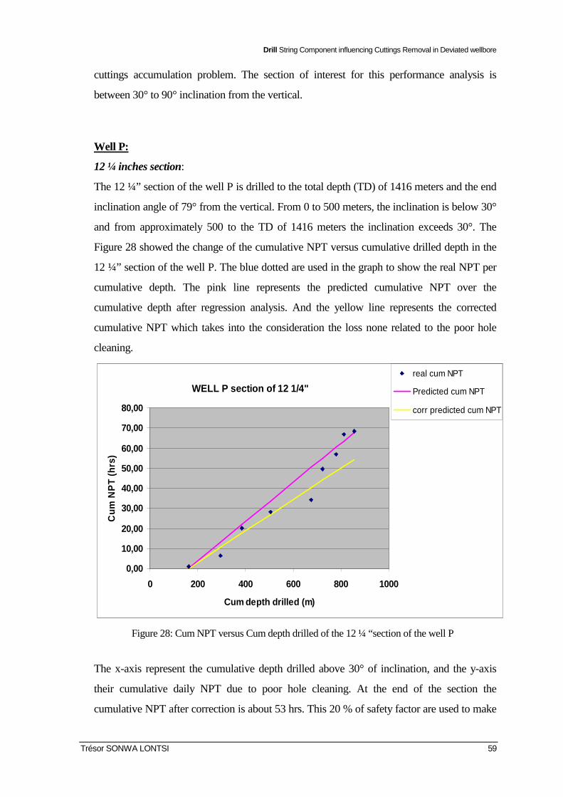
Drill String Component influencing Cuttings Removal in Deviated wellbore
Trésor SONWA LONTSI 59
cuttings accumulation problem. The section of interest for this performance analysis is
between 30° to 90° inclination from the vertical.
Well P:
12 ¼ inches section:
The 12 ¼” section of the well P is drilled to the total depth (TD) of 1416 meters and the end
inclination angle of 79° from the vertical. From 0 to 500 meters, the inclination is below 30°
and from approximately 500 to the TD of 1416 meters the inclination exceeds 30°. The
Figure 28 showed the change of the cumulative NPT versus cumulative drilled depth in the
12 ¼” section of the well P. The blue dotted are used in the graph to show the real NPT per
cumulative depth. The pink line represents the predicted cumulative NPT over the
cumulative depth after regression analysis. And the yellow line represents the corrected
cumulative NPT which takes into the consideration the loss none related to the poor hole
cleaning.
WELL P section of 12 1/4"
0,00
10,00
20,00
30,00
40,00
50,00
60,00
70,00
80,00
0 200 400 600 800 1000
Cum depth drilled (m)
Cum
NP
T (
hrs)
real cum NPT
Predicted cum NPT
corr predicted cum NPT
Figure 28: Cum NPT versus Cum depth drilled of the 12 ¼ “section of the well P
The x-axis represent the cumulative depth drilled above 30° of inclination, and the y-axis
their cumulative daily NPT due to poor hole cleaning. At the end of the section the
cumulative NPT after correction is about 53 hrs. This 20 % of safety factor are used to make

Drill String Component influencing Cuttings Removal in Deviated wellbore
Trésor SONWA LONTSI 60
the analyse more accurate because not all the reported back-reaming, wiper trip, etc… are
due to the poor hole cleaning.
The equation for the calculated pink line ( cumulative NPT) can be expressed as follows:
67,15*0979,0)( −= CumdepthhrsCumNPT (Eq.61)
And with the 20% safety factor the equation become:
54,12*0783,0)( −= CumdepthhrsCumNPT (Eq.62)
By comparing the factors that multiply the cumulative depth, we can be able to deduct the
efficiency of the hole cleaning in the section. So if we have less NPT this means that we also
have less hole cleaning problem, less time loss while drilling the section. And the figure
below shows us the behaviour of the NPT per meter each day.
The figure 29 (below) shows how the NPT varies per meter in this section. The three first
days we have an increase of the NPT/m, and which decrease again at the end of the section.
So no conclusion can be taking actually with this section.
Well section of 12 1/4"
0,000
0,050
0,100
0,150
0,200
0,250
0,300
0,350
0 200 400 600 800 1000
Cum depth drilled (m)
NP
T/m
(h
r/m
)
Real NPT/m
Figure 29: NPT per meter versus Cum depth drilled of the 12 ¼ “section of the well P
Cost analysis:
The following drilling cost due to the poor hole cleaning has been calculated for this critical
12 ¼” section, on the basis of well report time breakdown analysis for the well P.

Drill String Component influencing Cuttings Removal in Deviated wellbore
Trésor SONWA LONTSI 61
The prices uses in the economic evaluation are not standard, but just assume for the purpose
of this work. The 12 ¼” section of this well was drilled within a total of 9 days. The total
NPT during the 9 days are calculation and evaluate in cost in the table 6 (below):
Rig rate per day: 40,000 $/day
Daily production rate: 500 bbl/day
Days Drilled NPT(hours) NPT(days) NPT Cost
9 54,38 2,26 90.400$ Table 6: Cost of the NPT at the end of the section The late oil production interest of the field must also be estimated in order to give a good
idea about the total amount loss at end job by the operation company. The table 7 (below)
give of summarize of the cost and days losses:
Actual price per Barrel 90,00 $
Late production days 3,20
Production per day(bbl) 500 Loss production interest due
to poor hole cleaning 144.000 $ Late production interest
(10%) 14.400 $ Table 7: Total amount loss for the 12 ¼”section The total amount loss at the end of this section of the well is about 104.800 $ within 9 days
which represent a huge amount of money.
8 ½ inches section:
This section of the well H is drilled from 1416 meters to the Total Depth (TD) 2245 meters,
with 79° of inclination at the TD. The same linear regression analysis is made (i.e. the 12 ½”
section) with the 8 ½” hole section and the Cum NPT curve can be generated with the
equation:
609,17.*1306,0. −= depthCumNPTCum (Eq.63)
And with the safety margin of 20 % the equation will be as follow:
087,14.*1045,0. −= depthCumNPTCum (Eq.64)
Where,

Drill String Component influencing Cuttings Removal in Deviated wellbore
Trésor SONWA LONTSI 62
NPTCum. : represents the cumulative non-productive for a drilled interval cumulative
depthCum. : represents the cumulative interval drilled
The analyze of this field data start at the interval drilled above 30° of inclination which in
present situation is 143 meters. The graph in the figure 30 shows that at the end of the
drilling section, the cumulative NPT in the field based on the analysis used is about 65 hours.
The blue dotted are used in the graph to show the real NPT per cumulative depth. The pink
line represents the predicted cumulative NPT over the cumulative depth. And the yellow line
represents the corrected cumulative NPT which takes into the consideration the loss none
related to the poor hole cleaning.
WELL P section of 8,5"
0,00
20,00
40,00
60,00
80,00
100,00
120,00
0 200 400 600 800 1000
Cum depth drilled
Cu
m N
PT
Cum NPT
Predicted cum NPT
Corr predicted cum NPT
Figure 30: Cum NPT versus Cum depth drilled of the 8 ½ “section of the well P.
The figure 31 represents the NPT per meter of the section. The blue dotted points are the
NPT/meter in each interval drilled per day. The minimum NPT/meter is about 0.03 m/h for the
third day and 0.28 m/h reach in the 6 days.

Drill String Component influencing Cuttings Removal in Deviated wellbore
Trésor SONWA LONTSI 63
Well P section of 8,5"
0,00
0,05
0,10
0,15
0,20
0,25
0,30
0 200 400 600 800 1000
Cum depth drilled (m)
NP
T/m
(h
r/m
)Real cum m/hr
Figure 31: NPT per meter versus Cum depth drilled of the 8 ½ “section of the well P.
Cost analysis
For this section of the well, the job was done within 11 days.
The expenses due to the NPT are listed in the table 8 based on the same input as in the first
section. The table 8 summarizes the only NPT related to the poor hole cleaning action on the
rig site in 11 days drilled, and the corresponding additional rig cost.
Rig rate per day: 40,000 $/day
Daily production rate: 500 bbl/day
Days Drilled NPT(hours) NPT(days) NPT Cost
11 71,21 2,96 118.400 $ Table 8: Cost of the NPT at the end of the 8 ½”section The table 9 resumes the calculation of the total amount loss in this section of the well.
Assuming the price of a barrel oil today at 90,00 $, the late production interest after a certain
years of production will be add to the rig cost time to give us and idea of the total losses.
Actual oil price per Barrels 90,00 $
Late production days 3,28
Production per day(bbl) 500
Drill String Component influencing Cuttings Removal in Deviated wellbore
Trésor SONWA LONTSI 64
Loss production interest due to poor hole cleaning 147.600 $
Late production interest (10%) 14.760 $ Table 9: Total amount loss for the 8 ½”section The Total amount loss due to the hole cleaning and the late oil production interest of this 8
½”section is 118.400 $ for the 10 days required to drilled the section.
Well 2: well H
8 ½ inches section:
The well H is a deviated well with a TD of 2550 meters and with 67° of inclination angle at
the Total Depth. Only the 8 ½” section of this well is analysed because it is the section where
we can have hole cleaning problems based on the offset well drilled in the region. The other
sections of this well will not be of interest for the analysis. The daily NPT and the PT are
calculated in the same manner as in the well H. Based on the regression analysis, the
equation obtained can used for the 8 ½” section of this well. Per section, they are just one
equation that can be applied for the calculation of the cumulative NPT. This predicted line
obtained with the by plotting the cumulative NPT versus the cumulative interval depth
drilled is a tool for the comparison of the cleaning efficiency of the well.
The equation obtain for the predicted cumulative NPT is the follow:
345,7.*0470,0. −= depthCumNPTCum (Eq.65)
And with the safety margin of 20 % the equation will be as follow:
876,5.*0376,0. −= depthCumNPTCum (Eq.66)
Where,
NPTCum. : represents the cumulative non-productive for a drilled interval cumulative
depthCum. : represents the cumulative interval drilled
From the equation (with 20% safety), with the cumulative metrage drilled of 2030 meters,
the maximum NPT at the end of the section is about 70,44 hours. The blue dotted are used in
the graph to show the real NPT per cumulative depth. The pink line represents the predicted
cumulative NPT over the cumulative depth. And the yellow line represents the corrected
cumulative NPT which takes into the consideration the loss none related to the poor hole
cleaning.

Drill String Component influencing Cuttings Removal in Deviated wellbore
Trésor SONWA LONTSI 65
WELL H section 8,5"
0,00
20,00
40,00
60,00
80,00
100,00
120,00
140,00
0 500 1000 1500 2000 2500
Cum depth drilled (m)
Cu
m N
PT
Cum NPT
Predicted cum NPT
Corr Predicted cum NPT
Figure 32: Cum NPT versus Cum depth drilled of the 8 ½ “section of the well H
The graph of the figure 33 below represents the NPT per meter of this 8 ½” section. The
NPT/meter in this section is increasing with depth but varied depending of a lot of
parameters like formations, drilling practice, and also poor hole cleaning. The dotted points
represent the NPT/m drilled in each day. In this section the NPT/m has a tendency to
increase with drilled depth and inclination.
Well H section of 8,5"
0,00
0,02
0,04
0,06
0,08
0,10
0,12
0,14
0 500 1000 1500 2000 2500
Cum depth drilled (m)
NP
T/m
(h
r/m
)
Real NPT/m
Figure 33: NPT per meter versus Cum depth drilled of the 8 ½ “section of the well H

Drill String Component influencing Cuttings Removal in Deviated wellbore
Trésor SONWA LONTSI 66
Cost analysis
The 8 ½” open hole section of the oil well H was drilled in 17 days. The cumulative NPT is
converted into cost to be able to estimate the economic impact of the poor hole cleaning.
After having calculated the total NPT in this section of the wellbore, the total losses are
calculated based on following data (See also table 10):
Rig rate per day: 40,000 $/day Daily production rate: 500 bbl/day
Days Drilled NPT(hours) NPT(days) NPT Cost
9 70,44 2,94 117.600 $ Table 10: Cost of the NPT at the end of the 8 ½”section
They are addition cost due the late production of the well that must be taken into
consideration, which can be estimated as in the table 11:
Oil price per Barrels 90,00 $
Late production days(day) 2,40
Production per day(bbl) 500 Amount Loss due to poor
hole cleaning 108.000 $
Late production interest (10%) 10.800 $ Table 11:Total amount loss for the 8 ½”section of the well H
The total amount loss due to poor hole cleaning and late production interest of this well is
estimated at 128.400 $.
Well 3: Well G
The well G is drilled the starting depth of 1000 meters to the end at the TD of 1742 meters.
The maximum angle of the well path is about 45° and the target is reached at 30° of
inclination. The well in this section has a hole diameter of 12 ¼”, whereas the depth at about
1050 meters has 30° of inclination. The cumulative NPT is predicted based on the equation
obtained from the regression analysis with the equation:
410,0.*084,0. −= depthCumNPTCum (Eq.67)
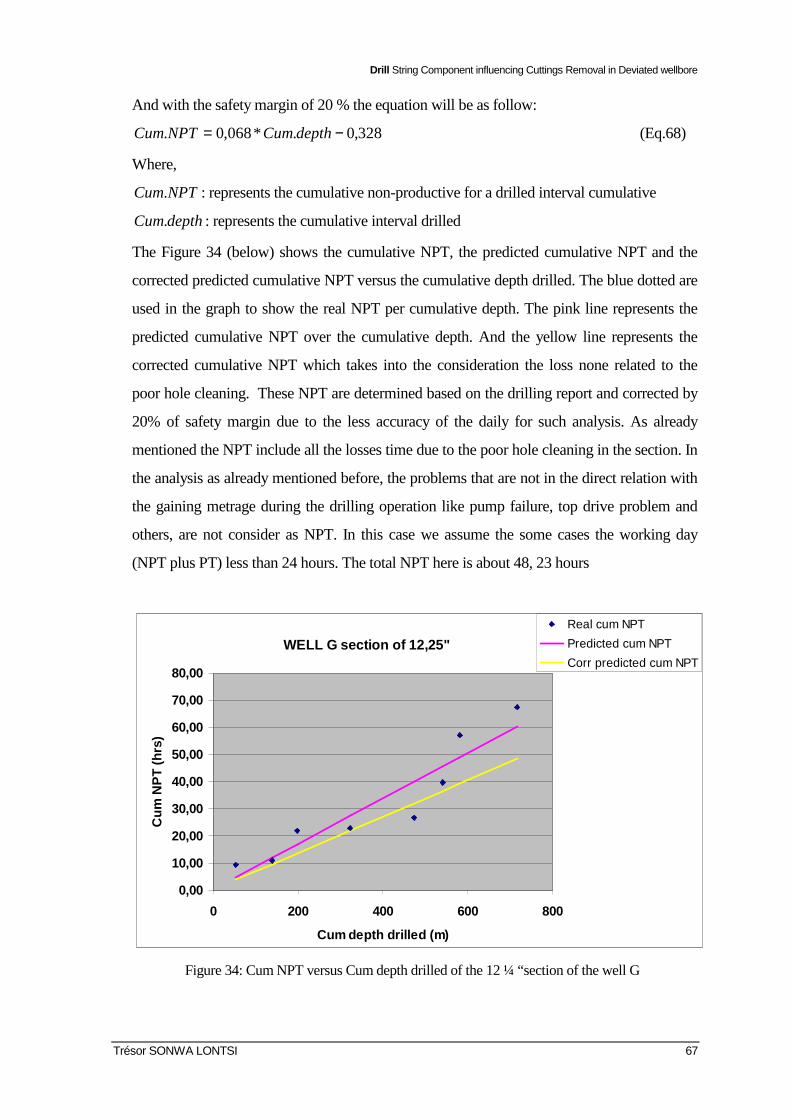
Drill String Component influencing Cuttings Removal in Deviated wellbore
Trésor SONWA LONTSI 67
And with the safety margin of 20 % the equation will be as follow:
328,0.*068,0. −= depthCumNPTCum (Eq.68)
Where,
NPTCum. : represents the cumulative non-productive for a drilled interval cumulative
depthCum. : represents the cumulative interval drilled
The Figure 34 (below) shows the cumulative NPT, the predicted cumulative NPT and the
corrected predicted cumulative NPT versus the cumulative depth drilled. The blue dotted are
used in the graph to show the real NPT per cumulative depth. The pink line represents the
predicted cumulative NPT over the cumulative depth. And the yellow line represents the
corrected cumulative NPT which takes into the consideration the loss none related to the
poor hole cleaning. These NPT are determined based on the drilling report and corrected by
20% of safety margin due to the less accuracy of the daily for such analysis. As already
mentioned the NPT include all the losses time due to the poor hole cleaning in the section. In
the analysis as already mentioned before, the problems that are not in the direct relation with
the gaining metrage during the drilling operation like pump failure, top drive problem and
others, are not consider as NPT. In this case we assume the some cases the working day
(NPT plus PT) less than 24 hours. The total NPT here is about 48, 23 hours
WELL G section of 12,25"
0,00
10,00
20,00
30,00
40,00
50,00
60,00
70,00
80,00
0 200 400 600 800
Cum depth drilled (m)
Cu
m N
PT
(h
rs)
Real cum NPT
Predicted cum NPT
Corr predicted cum NPT
Figure 34: Cum NPT versus Cum depth drilled of the 12 ¼ “section of the well G

Drill String Component influencing Cuttings Removal in Deviated wellbore
Trésor SONWA LONTSI 68
The blue dotted points represent the real cumulative NPT of this well. The pink line
represents the predicted cumulative NPT above 30° of inclination and the yellow line
represents the corrected predicted cumulative NPT. So we can see that the poor hole cleaning
really affect and increase the amount of the cost.
The figure 35 (below) represents the NPT per meter of the section. The blue dotted points
represent the NPT/m in each day. So in the first day, we have drilled almost 50 meters and
have lost 0, 04 hour per meter. This time loss is more related to the ROP than the inclination
angle in this case. The maximum NPT/m is about 0, 14 m/hr and the minimum at 0, 02 m/hr.
This NPT/meter doesn’t increase with the depth and inclination in this section. The goal of
this analyse is to finger out if the NPT/m will increase proportionally with the depth and
inclination?
Well G section of 12,25"
0,00
0,02
0,04
0,06
0,08
0,10
0,12
0,14
0,16
0 100 200 300 400 500 600 700 800
Cum depth drilled (m)
NP
T/m
(h
r/m
)
Real NPT/m
Figure 35: NPT per meter versus Cum depth drilled of the 12 ¼ “section of the well G
Cost analysis: This well was a geothermal well, so just the rig time losses will be consider for the economic
evaluation. The total NPT is also calculated and converted into cost. The table 12 shows the
total amount losses after 8 days required to drill the section.
Rig rate per day: 40,000 $/day

Drill String Component influencing Cuttings Removal in Deviated wellbore
Trésor SONWA LONTSI 69
Days Drilled NPT(hours) NPT(days) NPT Cost
8 48,23 2,01 80.400 $ Table 12: Cost of the NPT at the end of the 12 ¼”section The late production interest is not calculate in this well because is a geothermal well. The
total lost due to the poor hole cleaning of this hole in the 12 ½” section is about 80.400 $.
Result and conclusion:
The total NPT of the each of these three wells analyse above 30° inclination for this work is
significantly high. This result will increase the drilling cost and bring us to the question: if
this high NPT is due to the drilling practice, to the down hole drill string component used, or
both? After the economic evaluation of the three analysis in this thesis, it can be seen that the
hole cleaning must be further analyse in order to reduced this huge amount of loss. For these
reasons an alternative has to be found such as new drill string components to try to reduce
the drilling cost and the daily NPT. For this purpose, in the next chapter an economic
comparison between the losses due to the NPT while using Hydroclean Drill Pipe will be
analysed in the same area as well G, and H.
6.2 Wells drilled using HydroClean Drill Pipe
6.2.1 HydroClean
In order to optimize the hole cleaning performance, Weatherford has brought into the
industry a complete hole cleaning system. The improved system incorporates Hydroclean
technology, a tool to maximize the mechanical cuttings recirculation system. The
Hydroclean system has been developed in three different types, each integrating both the
Hydro-mechanical Cleaning Zones and Hydro-dynamical Bearing Zones, or only the profile
for hydro-mechanical cleaning. These tools are:
(1) Hydroclean Drill pipe which has the main functions as follows:
Optimized the hole cleaning
Reduced the differential sticking
Reduced torque and drag
Improved hydraulic performance

Drill String Component influencing Cuttings Removal in Deviated wellbore
Trésor SONWA LONTSI 70
(2) Hydroclean Heavy weight Drill pipe with almost the same functions as the drill pipe to:
Optimized the hole cleaning
Reduced the differential sticking
Reduced torque and drag
(3) and finally the Hydroclean Lo Torque Sub (will be not developed in this thesis) which,
Reduced torque and drag
Reduced the casing wear and can be used in cased or open hole
Design principles
The Hydroclean profile is designed with two different zones, the Hydro-mechanical
Cleaning Zone (HCZ) and the Hydrodynamic Bearing Zone (HBZ), which interact and
provide the two basic effects of the profile; hole cleaning and reduction of friction factor
between the bearing areas on the modified drilling equipment and the borewall.
By design principles, the Hydroclean profile is a combination of angles that work in
harmony to provide a number of affects resulting in the cuttings being re-introduced into
the flow stream.
There are two different alterations of flowing line patterns corresponding to the two
different zones of the profile, where there is a hydro-mechanical cleaning effect and a
hydrodynamic bearing effect. In order to have a better understanding of the effects
developed by the profiles, the following will firstly describe the principles of the
geometry.
Hydro-mechanical Cleaning Zone (HCZ)
The profile at the hydro-mechanical cleaning zone features three construction
angles, hcα , hcβ and hcγ angles. The geometry of this profile is composed of five
grooves, making the hcα angle relative to the x-axis of the equipment as shown in the
Figure below. These grooves are set at pre-determined angles to the axis of the drill pipe
and are optimized for normal drilling rotational speed between 80 rpm and 120rpm.The
grooves feature a hcβ negative angle, called negative leading edge angle, running in the
direction of the rotational speedΩ , while the opposite angle hcγ creates a positive
angle. The maximum outside diameter hcD of the Hydro-mechanical Cleaning Zone
(HCZ) is always smaller than the minimum diameter of the hydrodynamic bearing zone
(HBZ). This will ensure that the hydro-mechanical zone will never be in contact with

Drill String Component influencing Cuttings Removal in Deviated wellbore
Trésor SONWA LONTSI 71
the bore wall, as contact is at the larger diameter of the Hydrodynamic Bearing Zone
(HBZ).
Figure 36: Hydroclean Cleaning Zone (HCZ)
Hydrodynamic Bearing Zones (HBZ)
The profile of the Hydrodynamic Bearing Zone also has five grooves, which are aligned
with the five grooves of the Hydro-mechanical Cleaning Zone (HCZ). The
hydrodynamic bearing zone sections have positive edge angles 1θ and 2θ as also shown
in the Figure 34. The depth dhb, and width of the Hydrodynamic bearing zone grooves
decreases from inlet to outlet, in order to provide a continuous decrease of the passage
areas inside the grooves. The inlet groove on the hydrodynamic bearing zone is aligned
with the outlet groove on the hydro-mechanical cleaning zone. External grooves, at inlet
and outlet angles, enhance the geometric continuity between the external surfaces of the
drilling equipment and the profile itself. The helix angle hcα , of the hydro-mechanical
cleaning zone will be smaller than the helix angle hbα of the hydrodynamic bearing
zone. In order to have a continuous axial bearing while rotating the inclination
angle, hbα , of the profile ensures a ‘tight’ design configuration. This “nose coned”
shaped design are just on the second generation of the hydroclean, and are used to
decreases friction thanks to a fluid bearing effect between the pipe and the borehole.
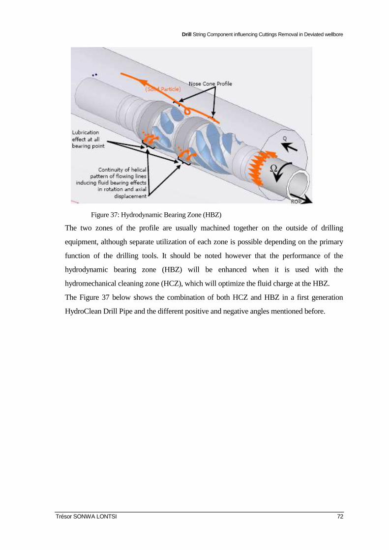
Drill String Component influencing Cuttings Removal in Deviated wellbore
Trésor SONWA LONTSI 72
Figure 37: Hydrodynamic Bearing Zone (HBZ)
The two zones of the profile are usually machined together on the outside of drilling
equipment, although separate utilization of each zone is possible depending on the primary
function of the drilling tools. It should be noted however that the performance of the
hydrodynamic bearing zone (HBZ) will be enhanced when it is used with the
hydromechanical cleaning zone (HCZ), which will optimize the fluid charge at the HBZ.
The Figure 37 below shows the combination of both HCZ and HBZ in a first generation
HydroClean Drill Pipe and the different positive and negative angles mentioned before.

Drill String Component influencing Cuttings Removal in Deviated wellbore
Trésor SONWA LONTSI 73
Figure 38: First generation HydroClean profile
Effect of Hydroclean on solid particles
The combined action of the rotational speed, the flow rate and the features of the HCZ and
HBZ will produce several effects on the cuttings lying on the low side of the wellbore like:
o Lifting effect: As the negative angle rotates over a solid particle, it is down up into
the groove by the venture effect created by the leading angle as in the Figure 35.
The particles are then held in this vortex and remains inside the groove cavity due to
the forces created by the vortex.

Drill String Component influencing Cuttings Removal in Deviated wellbore
Trésor SONWA LONTSI 74
Figure 39: Lifting effect of a solid particle
o Scoop effect: Almost similar to the lifting effect, the scoop effect is a simple
mechanical action where the negative angle digs into the bed and the particles are
scooped up and held in place by the same venture affect. This phenomenon is
illustrated in the Figure 40.
Figure 40: Scooped effect of a solid particle
o Archimedian Screw Effect: Once the particles have been held in place by the
venture effect, the rotation of the drill pipe will drive them upward. This archimedian
screw effect is enhanced as a result of working in combination with the negative
angle and the angle at which the angle at which the groove have been offset to the
pipes XX axis otherwise the particles would simply settle back to the low side of the
hole. This effect is also illustrated in the Figure 41 below.

Drill String Component influencing Cuttings Removal in Deviated wellbore
Trésor SONWA LONTSI 75
Figure 41: Archimedian screw effect of a solid particle
o Particle Boosting and Re-circulating: Here, the particles which are initially pulled
into the groove, are accelerated along the profile while sliding to the opposite side
where they are propelled and deflected back into circulation at an increased velocity
as a result of the combination of the archimedian screw effect, the actual rotation of
the drill pipe and the variable depth of the groove. This effect is illustrated in the
figure 42(below).
Figure 42: Re-circulation effect on a solid particle

Drill String Component influencing Cuttings Removal in Deviated wellbore
Trésor SONWA LONTSI 76
6.2.2 Application of HydroClean
The Hydroclean Drill Pipe has been specially designed to run in conjunction with the
standard drill pipe for use in extended reach well and other non –conventional wells. The
tool can be run in cased as also open hole wells without considerably increasing the friction
forces between the borehole wall and the pipe. The full length joint of 31 feet of the
hydroclean drill pipe has three central upset and his mechanical strength meets or exceeds
that of the S135 standard drill pipe. The hydroclean is suitable to be place one joint every 90
to 100 feet in problem area and in the inclination angle above 35 degrees from the vertical.
The heavy weight drill pipe hydroclean is also designed to be run along with conventional
heavy weight and a full length joint is composed of two central upset. The rugged design of
the two extended hydroclean sections makes it ideally suited to assist with hole cleaning in
the BHA. Experience for the Weatherford crew has shown that placing hydroclean heavy
weight as near as possible to the large outer diameter BHA components and one joint every
90 feet provides maximum hole cleaning performance.
HydroClean specification data
The hydroclean drill pipes and hydroclean heavy weight drill pipes (shown in Figure 43) are
constructed in different sizes, ranging from 3 ½ inches to 6-5/8 inches body outer diameter as
illustrated in the table 13. These data are very important in the field to avoid fishing problem
in case of a lost in the hole of one part of the hydroclean tool during the drilling process.
HYDROCLEAN DRILL PIPE Size
Feature 3 1/2 in 5 in 5 1/2 in 5 7/8 in 6 5/8 in A Body OD 3 1/2" 5" 5 1/2" 5 7/8" 6 5/8" B body ID 2 1/2" 4" 4 1/2" 4 3/4" 5 5/16" C Tool Joint OD 5" 6 5/8" 7" 7 1/4" 8" D Tool Joint ID (NC50) 2 1/4" 3" 3 1/2" 4 3/8" 4 1/4" E Dual OD 5 5/8" 7" 7 3/4" 8" 8 3/4" F Dual OD Length 6" 5 ½" 5 1/2" 5 1/2" 5 1/2" G Bearing Zone Length 8" 8" 8" 8" 8" H Bearing Zone OD 5 5/8" 7" 7 3/4" 8" 8 3/4" I Hydroclean Length 12" 12" 12" 12" 12" J Max. Hydroclean OD 5 1/8" 6 ½" 7 1/4" 7 1/2" 8 1/4" K Central Upset Spacing 7' 6" 7' 6" 7' 6" 7' 6" 7' 6" L Joint Length(ft) 31' 31' 31' 31' 31'
Table 13:HydroClean Drill Pipe specification

Drill String Component influencing Cuttings Removal in Deviated wellbore
Trésor SONWA LONTSI 77
Figure 43: Left Hydroclean Drill Pipe and right Hydroclean Heavy Weight
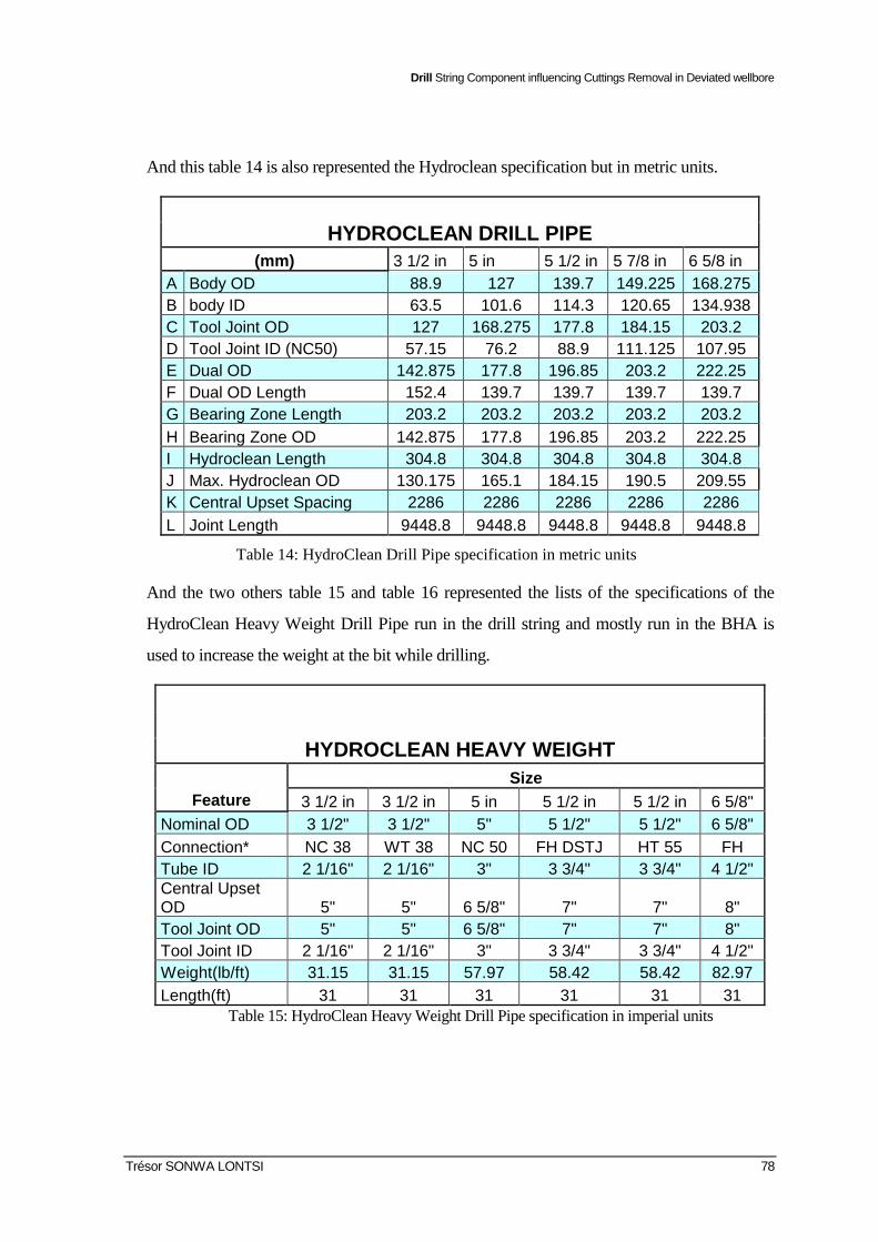
Drill String Component influencing Cuttings Removal in Deviated wellbore
Trésor SONWA LONTSI 78
And this table 14 is also represented the Hydroclean specification but in metric units.
HYDROCLEAN DRILL PIPE (mm) 3 1/2 in 5 in 5 1/2 in 5 7/8 in 6 5/8 in
A Body OD 88.9 127 139.7 149.225 168.275 B body ID 63.5 101.6 114.3 120.65 134.938 C Tool Joint OD 127 168.275 177.8 184.15 203.2 D Tool Joint ID (NC50) 57.15 76.2 88.9 111.125 107.95 E Dual OD 142.875 177.8 196.85 203.2 222.25 F Dual OD Length 152.4 139.7 139.7 139.7 139.7 G Bearing Zone Length 203.2 203.2 203.2 203.2 203.2 H Bearing Zone OD 142.875 177.8 196.85 203.2 222.25 I Hydroclean Length 304.8 304.8 304.8 304.8 304.8 J Max. Hydroclean OD 130.175 165.1 184.15 190.5 209.55 K Central Upset Spacing 2286 2286 2286 2286 2286 L Joint Length 9448.8 9448.8 9448.8 9448.8 9448.8
Table 14: HydroClean Drill Pipe specification in metric units
And the two others table 15 and table 16 represented the lists of the specifications of the
HydroClean Heavy Weight Drill Pipe run in the drill string and mostly run in the BHA is
used to increase the weight at the bit while drilling.
HYDROCLEAN HEAVY WEIGHT Size
Feature 3 1/2 in 3 1/2 in 5 in 5 1/2 in 5 1/2 in 6 5/8" Nominal OD 3 1/2" 3 1/2" 5" 5 1/2" 5 1/2" 6 5/8" Connection* NC 38 WT 38 NC 50 FH DSTJ HT 55 FH Tube ID 2 1/16" 2 1/16" 3" 3 3/4" 3 3/4" 4 1/2" Central Upset OD 5" 5" 6 5/8" 7" 7" 8" Tool Joint OD 5" 5" 6 5/8" 7" 7" 8" Tool Joint ID 2 1/16" 2 1/16" 3" 3 3/4" 3 3/4" 4 1/2" Weight(lb/ft) 31.15 31.15 57.97 58.42 58.42 82.97 Length(ft) 31 31 31 31 31 31
Table 15: HydroClean Heavy Weight Drill Pipe specification in imperial units

Drill String Component influencing Cuttings Removal in Deviated wellbore
Trésor SONWA LONTSI 79
HYDROCLEAN HEAVY WEIGHT Nominal OD 88.9 88.9 0 139.7 139.7 168.275 Connection* NC 38 WT 38 NC 50 FH DSTJ HT 55 FH Tube ID 52.388 52.388 76.2 95.25 95.25 0 Central Upset OD 0 127 168.275 177.8 177.8 203.2 Tool Joint OD 127 127 168.275 177.8 177.8 203.2 Tool Joint ID 52.388 52.388 76.2 95.25 95.25 114.3 Weight(kg/mm) 0.045 0.045 0.082 0.084 0.084 0.119
Length 9448.8 9448.8 9448.8 9448.8 9448.8 9448.8 Table 16: HydroClean Heavy Weight Drill Pipe specification in metric units
6.2.3 Field data analysis and result
One well drilled with HDP in the jungle of Peru in America was analysed to make a
technical and economical comparison with the wells drilled with Standard Drill Pipe. This
well was an oil field well and the characteristics of the well are as follow:
WELL C
The operator company of this well due to the experience of poor hole cleaning in the region
decided to use the HDP to increase the cuttings removal. The well is drilled from the KOP
200 meters to the TD of 3522 meters by Weatherford.
• At 880 meters we have an angle of 47° inclination and this is constant to the TD.
• The trajectory of the wellbore is a build and hold type and the inclination of 30° is
reach at 550 meters measured depth.
• The BHA was about 489 meters and with that BHA, the tangent section of 2952
meters MD was drilled.
• The flow rate was between 1700 and 2080 liters per minute and the rotation varied
from 80 to 110 rpm.
• Oil Based Mud with the specific gravity of 1, 38 SG was used and the pressure on
bottom was about 172 bars.

Drill String Component influencing Cuttings Removal in Deviated wellbore
Trésor SONWA LONTSI 80
• The formations was alternated between limestone, marl, shale and dense limestone in
this section
• The torque at the surface was between 19000 N-m and 22500 N-m.
• For drilling this well, 42 joints of 5” Hydroclean Drill Pipe (HDP) and 3 joints of
Hydroclean Heavy Weight Drill Pipe (HHW) were added to the drill string.
• 3 HHW run in the BHA and 42 HDP run from the top of a BHA 1350 meters (from
BHA) at a placement of 1 joint per stand.
12 ¼” section:
The 12 ¼” section was drilled from 200 meters to 2810 meters MD and the trajectory of the
section is a build and hold type. And the HDP was introduced at the end of the section,
because due to the poor hole cleaning, it was not possible to drill ahead with the same drill
string. The HDP is then used from 2404 to 2810 meters.
8 ½” section:
The 8 ½” section was drilled from 2810 meters to the Total Depth of 3522 with Hydroclean
Drill Pipe. The same BHA run as in the 12 ¼” section with 3 HHW was successfully used for
the rest of the holding section. The formations are alternated between limestone, marl, shale
and dense limestone in this section as in the well G an H. The figure 44 below shows the
profile of the well path of the well C and clearly shows were the HDP and SDP was used in
the wellbore.

Drill String Component influencing Cuttings Removal in Deviated wellbore
Trésor SONWA LONTSI 81
Figure 44: well profile of the WELL C
6.2.4 Limitations of HydroClean
• The HDP is a very expensive tools and the price of one joint of Hydroclean is 16
time the price of a Standard Drill Pipe.
• The HDP can not be rented or purchased by all the service companies
• The crew must be specially trained in order to be able to use Hydroclean during the
drilling process without problems.
• The placement of the Hydroclean joint in the Drill string increased the cuttings
removal, so the placement must be carefully done by the engineers in charge.
6.2.5 Economic Evaluation
Based on the drilling report and the drilling database of Weatherford, wells drilled with
Hydroclean Drill Pipe were down to the last detail analysed. The wellbore section with open
hole section of 12 ¼” and 8 ½” are the one of interest for this work. Like already done for
wells drilled with the SDP, the data for each section is grouped together and a linear
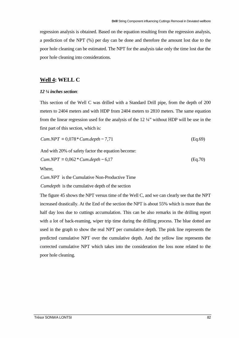
Drill String Component influencing Cuttings Removal in Deviated wellbore
Trésor SONWA LONTSI 82
regression analysis is obtained. Based on the equation resulting from the regression analysis,
a prediction of the NPT (%) per day can be done and therefore the amount lost due to the
poor hole cleaning can be estimated. The NPT for the analysis take only the time lost due the
poor hole cleaning into considerations.
Well 4: WELL C
12 ¼ inches section:
This section of the Well C was drilled with a Standard Drill pipe, from the depth of 200
meters to 2404 meters and with HDP from 2404 meters to 2810 meters. The same equation
from the linear regression used for the analysis of the 12 ¼” without HDP will be use in the
first part of this section, which is:
71,7.*078,0. −= depthCumNPTCum (Eq.69)
And with 20% of safety factor the equation become:
17,6.*062,0. −= depthCumNPTCum (Eq.70)
Where,
NPTCum. is the Cumulative Non-Productive Time
Cumdepth is the cumulative depth of the section
The figure 45 shows the NPT versus time of the Well C, and we can clearly see that the NPT
increased drastically. At the End of the section the NPT is about 55% which is more than the
half day loss due to cuttings accumulation. This can be also remarks in the drilling report
with a lot of back-reaming, wiper trip time during the drilling process. The blue dotted are
used in the graph to show the real NPT per cumulative depth. The pink line represents the
predicted cumulative NPT over the cumulative depth. And the yellow line represents the
corrected cumulative NPT which takes into the consideration the loss none related to the
poor hole cleaning.
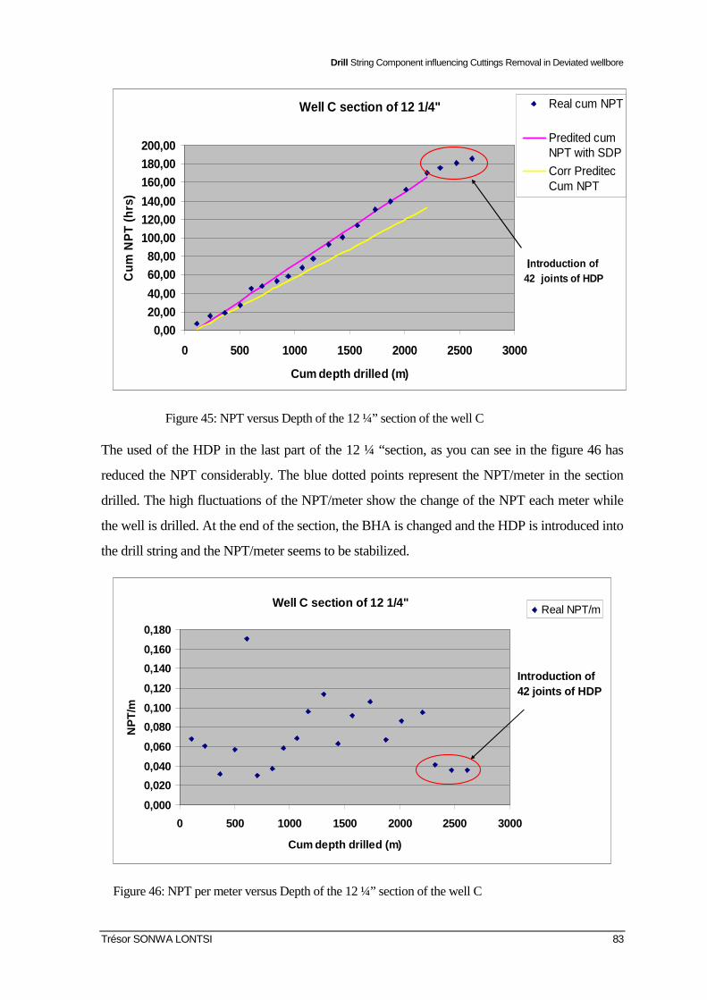
Drill String Component influencing Cuttings Removal in Deviated wellbore
Trésor SONWA LONTSI 83
Well C section of 12 1/4"
0,0020,0040,00
60,0080,00
100,00120,00140,00
160,00180,00200,00
0 500 1000 1500 2000 2500 3000
Cum depth drilled (m)
Cum
NP
T (h
rs)
Real cum NPT
Predited cumNPT with SDP
Corr PreditecCum NPT
Introduction of 42 joints of HDP
Figure 45: NPT versus Depth of the 12 ¼” section of the well C
The used of the HDP in the last part of the 12 ¼ “section, as you can see in the figure 46 has
reduced the NPT considerably. The blue dotted points represent the NPT/meter in the section
drilled. The high fluctuations of the NPT/meter show the change of the NPT each meter while
the well is drilled. At the end of the section, the BHA is changed and the HDP is introduced into
the drill string and the NPT/meter seems to be stabilized.
Well C section of 12 1/4"
0,000
0,020
0,040
0,060
0,080
0,100
0,120
0,140
0,160
0,180
0 500 1000 1500 2000 2500 3000
Cum depth drilled (m)
NP
T/m
Real NPT/m
Introduction of 42 joints of HDP
Figure 46: NPT per meter versus Depth of the 12 ¼” section of the well C
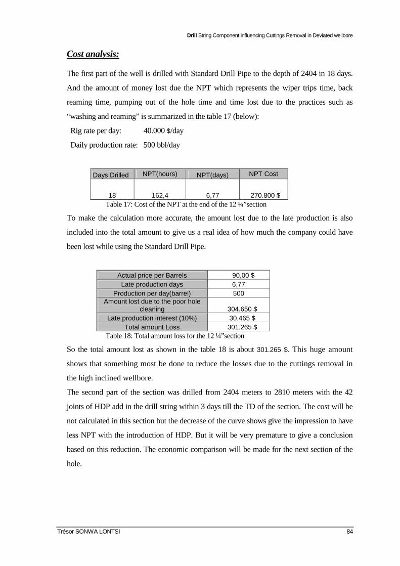
Drill String Component influencing Cuttings Removal in Deviated wellbore
Trésor SONWA LONTSI 84
Cost analysis:
The first part of the well is drilled with Standard Drill Pipe to the depth of 2404 in 18 days.
And the amount of money lost due the NPT which represents the wiper trips time, back
reaming time, pumping out of the hole time and time lost due to the practices such as
“washing and reaming” is summarized in the table 17 (below):
Rig rate per day: 40.000 $/day
Daily production rate: 500 bbl/day
Days Drilled NPT(hours) NPT(days) NPT Cost
18 162,4 6,77 270.800 $ Table 17: Cost of the NPT at the end of the 12 ¼”section
To make the calculation more accurate, the amount lost due to the late production is also
included into the total amount to give us a real idea of how much the company could have
been lost while using the Standard Drill Pipe.
Actual price per Barrels 90,00 $ Late production days 6,77
Production per day(barrel) 500 Amount lost due to the poor hole
cleaning 304.650 $ Late production interest (10%) 30.465 $
Total amount Loss 301.265 $ Table 18: Total amount loss for the 12 ¼”section
So the total amount lost as shown in the table 18 is about 301.265 $. This huge amount
shows that something most be done to reduce the losses due to the cuttings removal in
the high inclined wellbore.
The second part of the section was drilled from 2404 meters to 2810 meters with the 42
joints of HDP add in the drill string within 3 days till the TD of the section. The cost will be
not calculated in this section but the decrease of the curve shows give the impression to have
less NPT with the introduction of HDP. But it will be very premature to give a conclusion
based on this reduction. The economic comparison will be made for the next section of the
hole.

Drill String Component influencing Cuttings Removal in Deviated wellbore
Trésor SONWA LONTSI 85
8 ½ inches section
The 8 ½” section of this well was drilled with the HDP into the 9 5/8” casing from the
starting depth of 2810 meters to the TD of 3522 meters. The well was drilled within 6 days
and the cumulative NPT is predicted based on the equation obtains from the regression
analysis. This equation is expressed as follow:
47,2.*014,0. −= depthCumNPTCum (Eq.71)
And with 20% of safety factor the equation become:
97,1.*011,0. −= depthCumNPTCum (Eq.72)
Where,
NPTCum. is the Cumulative Non-Productive Time
Cumdepth is the cumulative depth of the section
As shows in the figure 47 below, after the correction of 20 % safety margin, the cumulative
NPT at the end of the section is about 11 hours. The blue dotted are used in the graph to
show the real NPT per cumulative depth. The pink line represents the predicted cumulative
NPT over the cumulative depth. And the yellow line represents the corrected cumulative
NPT which takes into the consideration the loss none related to the poor hole cleaning. We
can clearly see that the Hydroclean give low value of the daily NPT which decrease the total
drilling cost and time of the well.

Drill String Component influencing Cuttings Removal in Deviated wellbore
Trésor SONWA LONTSI 86
Well C section of 8,5"
0,00
2,00
4,00
6,00
8,00
10,00
12,00
14,00
16,00
0 200 400 600 800 1000 1200
Cum depth drilled (m)
Cu
m N
PT
(h
rs)
Real NPT
Predicted cum NPT
Corr predicted cum NPT
Figure 47: Cum NPT versus Cum Depth of the 8 ½” section of the well C with SDP and HDP
And the figure 48, the blue dotted points represent the cumulative metrage per meter over the
cumulative depth. This graph gives us the possibility to identify whether or not is the NPT is
proportionally increased with the depth. In the cumulative depth of almost 600 meters
drilled, the NPT/meter high than the cumulative depth of 820 meters. As a conclusion while
looking at the graph and at the figure 47, the NPT/meter increase even smoothly, with
increasing depth. This section is a hold section which don’t take the increase of the
inclination into consideration because the inclination stays the same till the TD. In the build
section as already mentioned before we have more fluctuations of the NPT/meter.

Drill String Component influencing Cuttings Removal in Deviated wellbore
Trésor SONWA LONTSI 87
Well C section of 8,5"(m/hr)
0,000
0,005
0,010
0,015
0,020
0,025
0,030
0 200 400 600 800 1000 1200
Cum depth drilled(m)
cum
met
rag
e d
rille
d(m
/hr)
Real cum m/hr
Figure 48: NPT per meter versus Cum Depth of the 8 ½” section of the well C with SDP and HDP
Cost analysis:
The economic comparison between Hydroclean and Standard Drill Pipe done in this part of
the work give us the amount saved. Based on my result the company will be able to make a
good choice by using one of the two down hole equipments. The company can either rented
or purchased the HDP depending on their internal policy. Both possibilities are taken into
consideration in our calculation. The section was as already mentioned drilled from 2810
meters to the TD of 3522 meters in 6 days with HDP. The input data for the calculation are
presented in table 19 below:
Days required to drill the section 6
Oil price per barrel 90 $
Barrels oil production expected per day 500
Rig rate per day 40.000 $
Number of HDP joint used for the section 45
Rental charges of HDP per joint per day 48 $
Purchasing cost of HDP per joint per day 16 $ Table 19: Input data for lost cost calculation
So if the company purchased the Hydroclean, the average life per joints is approximately 730
days and the purchasing cost per joint around 12000 $, which lead to the 16 $/day per joint.

Drill String Component influencing Cuttings Removal in Deviated wellbore
Trésor SONWA LONTSI 88
With the others given prices, the savings cost when drilling with the HDP instead of the
Standard Drill Pipe can be calculated and summarized in table 20 as follow:
Actual price per Barrels 90,00 $ Late production days 0.46
Production per day(barrel) 500 Amount lost due to the poor hole
cleaning 3.726 $ Late production interest (10%) - $
Total amount Loss 40.000 $ Table 20: Total saved with HDP
The total amount loss in this section after 6 drilled days is approximately half of a day.
This total amount is estimated at 40.000 $ which represent one day of rent the rig.
Conclusion:
Comparing the wells drilled in the same area as Well C, G and H, following can be observed:
In the 8 ½ “section, well H and C give the equation:
876,5.*0376,0. −= depthCumNPTCum , drilled with Standard Drill Pipe
97,1.*011,0. −= depthCumNPTCum , drilled with Hydroclean Drill Pipe
By comparing the two equations we can come to the conclusion that in this case the HDP give
us less NPT for this section.
In the 12 ¼” section, well C is partially drilled with HDP, and well G totally with SDP and the
resulting equation from the linear equation are:
328,0.*068,0. −= depthCumNPTCum , drilled with Standard Drill Pipe
17,6.*062,0. −= depthCumNPTCum , partially drilled with Hydroclean Drill Pipe
Even in this case we can see the effect of the HDP in the 12 ¼” section.
But this conclusion can not be valid for all the wells, because as we can see in the well P the 8
½” and 12 ¼” section, the comparison can not be made. This well P was drilled in another
country with different formations.

Drill String Component influencing Cuttings Removal in Deviated wellbore
Trésor SONWA LONTSI 89
6.3 Cuttings Bed Impellers
6.3.1 Definition of the Cuttings Bed Impellers (CBI)
The build up of the cuttings in high angle wells can cause drill pipe wear, hole instability,
excessive torque and drag. These problems lead to the development of the CBI. Cuttings Bed
Impeller is a down hole drill string tool intended for use in deviated wells where excessive
build up of cuttings causes drilling problems.
The CBI is an integral drill string component consisting of a short mandrel with no moving
parts, shaped in such a way as to stimulate any cuttings which have a tendency to settle out of
the mud in the high angled sections of the well bore. The high angled sections could be
inside the casing or in open hole: the tool is adaptable to suit several environments. The
illustration of the CBI is shown in the figure below:
The Chevron shaped blades to ensure effective cuttings agitations in both directions
The Incut zone designed as we can see in the figure to encourage loosening of
cuttings beds and allow for flexibility in the mandrel
End the mandrel strength matches maximum strength of drill pipe toll joint.
Features
The features of the CBI (see figure 49) are as follow:
One piece mandrel with mechanical properties which exceed the drill pipe in which
it is placed
Dimensions which allow the use of up to two tools within a standard drilling stand in
most drilling derricks
Hydraulic and mechanical dual acting mechanisms to remove cuttings beds
Tool can be dressed with different coatings according to the severity of the down
hole conditions.
The CBI are available in the size of 3 ½” , still 6-5/8” outer diameter and their mechanical
data are given in the table 21 (below) and even one comparison between a new 5” S135
string and a new 5” CBI.

Drill String Component influencing Cuttings Removal in Deviated wellbore
Trésor SONWA LONTSI 90
Figure 49: Representation of the Cuttings Bed Impellers
Descriptin 3-1/2” 4" 5" 5-1/2" 6-5/8" Standard connection 2-7/8"IF 3-1/2"IF 4-1/2"IF 5-1/2"IF 6-5/8"FH Min. Make Up
Torque Ft-lbs 13,5 15 28 43,5 54 Overall
Length(sh-sh) in 42.5 45.375 40.50 40.50 40.50
Body
Tool Joint O.D. in 5.25 6 6,5 7.375 8.20
Tool Joint I.D. in 2.13 2.13 3.25 3.25 4.25
Maximum Body O.D in 5.5 6.25 7.40 7.75 8.50
Length of Fish Neck in 11 11 10,5o 10.50 10.50
Tensile Yield Lbs 802,814 954,317 1,336,600 1,656,900 1,592,100 Torsional Yield Ft-lbs 47,975 56,325 115,9 145,3 173,5
Table 21: Cuttings Bed Impellers specification

Drill String Component influencing Cuttings Removal in Deviated wellbore
Trésor SONWA LONTSI 91
Description New 5" S135
New 5" CBI
Standard connection 4-1/2"IF 4-1/2"IF Min. Tool Joint O.D. in 6,68 6,5 Min. Tool Joint I.D. in 2,75 3,25 Minimum Make Up Torque Ft-lbs 32,21 28 Tensile Yield Lbs 1,551,706 1,268,900 Torsional Yield Ft-lbs 62,387 51,4
Body
Minimum Body O.D in 5 5,25 Minimum Body I.D in 4,275 3,25 Overall Length(sh-sh) in 30.00 40.25 Tensile Yield Lbs 710 1,336,600 Torsional Yield Ft-lbs 77,4 115,9
Table 22: 5” Cuttings Bed Impellers and 5” Standard Drill Pipe comparison
6.3.2 Applications of the CBI
Basically the Cuttings Bed Impeller (CBI) is a down hole drill string intended to agitate any
cuttings accumulation which have the tendency to settle out of the mud in deviated wells
above 30° inclinations where excessive build up of cuttings causes drilling problems. The
CBI can be use inside the casing section as also in the open hole section. The CBI tool is
designed so that the coating over the top of the blades is suitable for both applications inside
casing and in open hole. When running the tools primarily inside casing the coating has a
low friction property to reduce casing wear. And running in the open hole the same hard,
abrasive resistant coating allows for extended run lengths in arduous wellbore condition. The
figure 50 (below) showed the typical case where cuttings have fallen out of the mud and
have come to rest just below the build section and the action of the CBI to agitate cuttings
into the flow mud. The most effective spacing of the CBI down hole tools is normally
between 91 meters and 152 meters20 through the tangent section of the well trajectory, which
can ensure the re-agitation and the re-introduction into the mud flow of the cuttings build at
the low side. The flow pattern of the returning mud around the tool annulus has been
optimized to ensure maximum lifting of the debris from the low side of the hole.

Drill String Component influencing Cuttings Removal in Deviated wellbore
Trésor SONWA LONTSI 92
Figure 50: mechanical agitation of cuttings bed with the CBI
6.3.3 Advantages and Limitations of the CBI
Some benefits of the CBI are to:
Reduces torque and drag on the string while in drilling mode which is not always
easy to achieve in deviated wellbore
Reduces wear on the drill pipe and rotating equipment
Ensures cleaner and more stable hole conditions
Reduces the drilling costs
Only a small number of tools are required for effective hole cleaning
Acts as a vibration damper in the string
Overcomes difficulties in sliding and increase the rate of penetration
Reduces frequency of twists-off and stuck pipe
And one of the major limitations of the tools is that we have a lot of connections due to the
short length of the CBI. This will increase first the connection time and increase the
possibility of losses into the hole.
Drill String Component influencing Cuttings Removal in Deviated wellbore
Trésor SONWA LONTSI 93
6.4 Helical Drill Pipe
6.4.1 Definition and features
The Helical Drill Pipe (HE-DP) is a future alternative approach to overcome cuttings
accumulation problems in high angle and horizontal wells. Compared to conventional drill
pipe this helical pipe requires an additional manufacturing step, during which the major
portion of the pipe body is transformed into an internally and externally helical tube, shaped
similar to the rotor of a multi lobe mud motor. Drill pipe segments required for slips and
elevators, the upset areas at both ends and the tool joints remain circular in shape. The
minimum internal diameter of this helical section is at least as large as the internal diameter
of the tool joint. The maximum outer diameter of the helical section is close to or identical to
the outer diameter of the tool joints as you can see in the figure 51 illustrating the design of
the Helical Drill Pipe.
Figure 51: Design of Helical Drill Pipe
Helically shaped “multi-lobe” drill pipe improves the transport of cuttings in highly inclined
and horizontal sections of the well both in the rotating and sliding mode of steerable systems.
In highly inclined or horizontal sections drilled with conventional drill pipe the annulus
between drill string and borehole wall is considerably reduced by cuttings deposited in the
form of cuttings beds. Helical pipe considerably reduces the amount of solids deposited at

Drill String Component influencing Cuttings Removal in Deviated wellbore
Trésor SONWA LONTSI 94
the low side of the hole. The Figure 52 illustrates the HE-DP in case of differential sticking.
Because of the unconventional shape of the helical pipe the contact between pipe and
borehole wall is only a fraction of the contact between round and conventional bore hole
elements with spirally milled groves.
Figure 52: Cross section of Helical Drill Pipe in the borehole
6.4.2 Advantages of Helical Drill Pipe
The advantages of this pipe will be comparing with standard Drill pipe like:
The net annular flow area around helically enhanced drill pipe vs. conventional pipe is
increased because of the lack of an obstruction by settled solids, thus reducing the pressure
drop in the annulus.
Torque and Drag are minimized hand in hand with the reduction or elimination of
cuttings beds. Less wear an tear on surface and down hole equipment, lower energy
consumption and an increased potential to reach more distant targets with existing
equipment are the consequence.
Because of the unique construction the average time between the generation of
cuttings at the bit and the appearance at the shale shaker is considerably reduced
because of the elimination of sedimentation at the low side of the hole. Mud
rheology and density can be controlled easier and more cost effective when re-
drilling of cuttings between drill string and borehole wall is reduced.
Poor cementing jobs resulting from annular sections partially filled with deposited
cuttings can be avoided.
The need for wiper trips, back reaming, pumping out of the hole and practices
already mentioned in this work can be minimized.

Drill String Component influencing Cuttings Removal in Deviated wellbore
Trésor SONWA LONTSI 95
The price of a joint of Helical Drill Pipe is less than one joint of HDP
6.4.3 Limitations of the Helical Drill Pipe
One of the major question while using Helical Drill Pipe is the fishing of the tools in case of
lost in the hole. But this situation can be solved as follows:
External Engagement with Overshots
Helical pipe can be engaged by conventional overshots with a bull nose attached to the top
sub that enters the pipe to prevent it against radial deformation when engaging the helix with
the grapple
Internal Engagement with Spears:
Spears can be set inside the helical sections and for maximum pulling loads in the circular
section of a joint of pipe (tool joints, upset area or slip and elevator area)
The availability of the Helical Drill pipe can be also an issue to solve when deciding the run
it for a section.

Conclusion and Recommendations
Trésor SONWA LONTSI 96
7 Conclusion and Recommendations
7.1 Conclusion
At the rig site while drilling deviated wells, poor hole cleaning can most of the time be
identify by the following events:
• High torque on the drill string which result from the resistance to the rotation of the
drill string
• Excessive drag on the drill string while tripping which result from the resistance to
reciprocation
• And the type and quality of the cuttings at the shale shaker
The major drilling operating parameters influencing the hole cleaning are the flow rate, flow
regime, the drilling mud properties and drill pipe rotation. These drilling parameters are
controllable and can be optimized to increase the cuttings transport in deviated wells.
So, determining the optimum flow rate for good cuttings transport must be done in the well
planning phase and must be adjusted as the real time during the drilling phase of the
wellbore. If the optimum flow rate is below the minimum annular velocity, increase it until
all annulus sections have a velocity greater than, or equal to, the minimum allowed.
Back-reaming and wiper trip for hole cleaning issues must be reduced, even avoided as
possible on the rig site. The drilling operators have taken them as a normal drilling practice.
The use of HDP in deviated wells must be follow by the “best” drilling practice in order to
give the expected good cleaning result. But the availability of the HDP must be carefully
checked before deciding to run them for a section.
Based on the analysis did in this work, when comparing well G, H and well C, the linear
regression shows less NPT for the well C drilled with HDP. The well P compare with the
well C shows less NPT. This led to the conclusion that the NPT can not be reduced only with
HDP, and is also depending on the formation drilled. There are many factors like formations,
drilling practices that must be taken into consideration.

Conclusion and Recommendations
Trésor SONWA LONTSI 97
7.2 Recommendations
Based on the results from oldest studies used for this thesis and from various field
experiences the following general guidelines can be recommended to partially solve the
cuttings accumulation problem in high deviated wells:
Design if possible the well path of the section as smooth as possible so that we can
avoid critical angles and high dogleg.
Maximize fluid velocity in the annulus, while avoiding hole erosion, by increasing
pumping power and/or using large diameter pipes and collars.
In large diameter horizontal wellbores, where turbulent flow is not practical, use mud
with high suspension properties and mud with high meter dial readings at shear rates
Pump Hi-viscosity and Low-viscosity pills at the right time, and adjust the plastic
viscosity and yield point as per recommendation in the section.
More analysis must be done in future research in order to come out with a definitive
conclusion, of whether the HDP can be more effective by reducing the NPT in all high
deviated wells rather than SDP.

Nomenclatures
Trésor SONWA LONTSI 98
8 Nomenclatures
bedA : Cross-section flow area of the cutting bed in sqft
wA : Cross-section flow area of the wellbore in sqft
newannA − : New annular area after cuttings deposition
cC : Feed cuttings concentration
concC : Concentration correction factor
angC : Angle correction factor
sizeC : Cuttings size correction factor
RPMC : RPM correction factor
Ci : Angle correction factor for the new cutting lifting equation
MWC : Density or mud weight correction factor
bedC : Cuttings bed
cuttC : Corrected cuttings bed concentration
cuttC : Cuttings bed concentration
cuttcorrC − : correction factor of cuttings bed
holeD : Hole diameter in inches
Dpipe : Pipe diameter in inches
K : Consistency index, dimensionless
α : Angle in degree versus vertical
ReN : Reynolds number
FrN : Froude number
minQ : Minimum flow rate to keep the hole clean
pumpQ : Pump flow rate
Rt : Cuttings transport ratio
Vslip : Slip velocity
Vcut : Cuttings velocity

Nomenclatures
Trésor SONWA LONTSI 99
newcutV − : New cuttings velocity
minV : Minimum velocity
Vopen : Velocity of the open area above the cuttings bed
Vann : Annular velocity
µ : Mud viscosity at shear rate in flow stream in centipoise
v : Annular velocity, ft/min
mudρ : mud weight, ppg
pρ : particle density, ppg
n : Flow index, dimensionless
θ300 : 300 viscometer dial reading
θ600 : 600 viscometer dial reading
yτ : Shear stress in pounds per square inches
sρ : Solid density in pounds per gallon
fρ : Fluid density in pounds per gallon
aµ : Apparent fluid viscosity in centipoise
annν : Annular velocity in feet per minute
sd : Solid diameter in inches
yτ : Shear stress
ABBREVIATIONS:
Abs : Absolute value of
ANN : Artificial Neural Network
BHA : Bottom Hole Assembly
CBI : Cuttings Bed Impellers
Cum Depth: Cumulative Depth in meters
Cum NPT: Cumulative Non Productive Time in hours
ESV : Equivalent Slip Velocity
ID : Internal Diameter
gpm : Gallon per minute

Nomenclatures
Trésor SONWA LONTSI 100
HBZ : Hydrodynamical Bearing Zone
HCZ : Hydromechanical Cleaning Zone
HDP : Hydroclean Drill Pipe
HE-DP: Helical Drill Pipe
KOP : Kick Of Point
LSRV: Low Shear Rate Viscosity
LSYP: Low Shear Yield Point
MD : Measured Depth
NPT : Nom Productive Time
OD : Outer Diameter
PT : Productive Time
ppg : Pounds per gallon
RSS : Rotary Steerable System
ROP : Rate Of Penetration
RPM : Rotation Per Minute
SG : Specific Gravity of the mud
SDP : Standard Drill Pipe
TD : Total Depth

References
Trésor SONWA LONTSI 101
9 References
1. Drilling Engineering by Jamal, J. Azar, G. Robello Samuel
2. J. Azar et al. “Important Issues in Cuttings Transport for Drilling Directional Wells”
paper SPE 39020.
3. W.B Bradley et al. ”Task Force Approach to Reducing Stuck Pipe Cost“ paper SPE
21999 presented in March 1991
4. Rudi Rubiani et al. “Equation for Estimating Mud Minimum Rate for Cuttings
Transport in an Inclined-until-Horizontal Well”, paper SPE/IADC 57541 presented at
November 1999
5. S.A. Mirhaj et al. “Cuttings Removal Simulation for Deviated and Horizontal
Wellbores” paper SPE 105442 presented Middle East Oil & Gas Sow and Conference,
11-14 March 2007
6. Larsen et al. ”Development of a new cuttings transport Model for High-Angle
Wellbores Including Horizontal Wells” paper SPE presented in June 1997
7. A.A. Pilehvari et al.“ State of the Art Cuttings Transport in Horizontal Wellbores”
paper SPE, presented in September 1999
8. David Power, Deepwater Technical Advisor “Hole Cleaning: Challenges and
Solutions”
9. Exxon Company, USA “Drilling Fluid Technology”
10. Baker Hughes INTEQ “Drilling Engineering Workbook”
11. M.I Swaco “ Drilling Fluid Engineering Workbook”

References
Trésor SONWA LONTSI 102
12. Hyon cho et al. ” A Three Segment Hydraulic Model for Cuttings Transport in
Horizontal and Deviated wells” paper SPE presented in November 2000
13. R.K. Clark et al. “ A mechanistic Model for cuttings Transport” paper SPE 28306
presented in September 1994
14. Tomren, P.H., Iyoho, A.W.,and Azar, J.J.: “Experimental Study of Cuttings Transport
in Directional Wells,” paper SPE presented in August 1986
15. Zeidler U. and Rice U. “An Experimental Analysis of the Drillied Transport of Drilled
Particles” paper SPE 3064 presented in Houston in February 1986
16. Ozbayoglu et al. “ Analysis of Bed Height in Horizontal and Highly Inclined Wellbores
by Using Artificial Neural Networks” paper SPE 78939 presented in Alberta in
November 2002
17. Gavignet and Sobey “ Models Aids Cuttings Transport Predictions” paper SPE 15417
presented in September 1989
18. Pilehvari, A.A., Azar, J.J. and Shirazi, S.A. “State-of-the-Art Cuttings Transport in
Horizontal Wellbores”, paper SPE presented in September 1999
19. Kamp, A.M. and Rivero, M. “Layer Modeling for Cuttings Transport in Highly Inclined
Wellbores”, paper SPE 53942 presented in September 1999
20. Pilot drilling Control Ltd handout
21. Desmond Nguyen and S.S. Rahman, “A Three Layer Hydraulic Program for Effective
Cuttings Transport and Hole Cleaning in Highly Deviated and Horizontal Wells” ,
paper SPE 51186 presented in March 1998

References
Trésor SONWA LONTSI 103
22. Okrajni and J.J Azar, “ The Effects of Mud Rheology on Annular Hole Cleaning in
Directional Wells” paper SPE 14178 presented in 1986
23. Sifferman and T.R. Becker, “Hole Cleaning in Full-Scale Inclined Wellbores” paper
SPE 20422 presented in March 1992
24. Martins and C. Santana “Evaluation of Cuttings Transport in Horizontal and Near-
Horizontal –A Dimensionless Approach” paper SPE 23643 presented in March 1992
25. Belavadi and G.A. Chukwu, “ Experimental Study od the Parameters Affecting Cutting
Transportation in a Vertical Wellbore Annulus” paper SPE 27880 presented in March
1994
26. Kenny and al. “Hole Cleaning Modelling: What’s ‘n’ Got To Do With It?” paper SPE
35099 presented in March 1996
27. Sanchez, J.J. Azar, A.A Bassal, A.L. Martins “Effect of Drill Pipe Rotation on Hole
Cleaning during Directional Well Drilling” paper SPE 56406 presented in June 1999
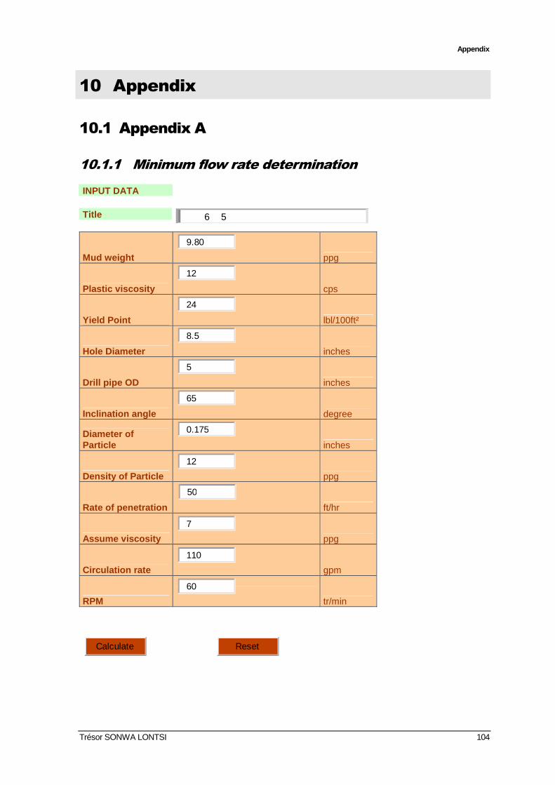
Appendix
Trésor SONWA LONTSI 104
10 Appendix
10.1 Appendix A
10.1.1 Minimum flow rate determination
INPUT DATA Title
Mud weight
ppg
Plastic viscosity
cps
Yield Point
lbl/100ft²
Hole Diameter
inches
Drill pipe OD
inches
Inclination angle
degree
Diameter of Particle
inches
Density of Particle
ppg
Rate of penetration
ft/hr
Assume viscosity
ppg
Circulation rate
gpm
RPM
tr/min
12
24
8.5
5
65
12
6 5
Calculate Reset
9.80
0.175
50
7
110
60

Appendix
Trésor SONWA LONTSI 105
OUTPUT VARIABLES
Cutting concentration 2,397
Velocities (ft/min.)
♦ cuttings 1,424473125
♦ ESV 3,257867993
♦ minimum 9,701267753
♦ Qmin(gpm) 584,1024938
10.1.2 Visual Basic Application (VBA)
Dim X As Double
Static Function Log10(X)
Log10 = Log(X) / Log(10#)
End Function
Private Sub CommandButton1_Click()
Const c = 12
Dim arr(1 To c) As Double
Dim Cconc As Double
Dim Vcut As Double
Dim Vmin As Double
Dim ESV As Double
Dim Qmin As Double
Dim i As Double
Dim n As Double
Dim k As Double
Dim mu As Double
Dim NRE As Double
Dim f As Double

Appendix
Trésor SONWA LONTSI 106
Range("B5").Select
arr(1) = TextBox1.Value ' Mud weight
arr(2) = TextBox2.Value 'Plastic viscocity
arr(3) = TextBox3.Value 'Yield point
arr(4) = TextBox4.Value 'Hole diameter
arr(5) = TextBox5.Value 'pipe diameter
arr(6) = TextBox6.Value 'inclination angle
arr(7) = TextBox7.Value 'diameter of particle
arr(8) = TextBox8.Value 'density of particle
arr(9) = TextBox9.Value 'rate of penetration
arr(10) = TextBox10.Value 'ESVassume
arr(11) = TextBox11.Value 'circulation rate
arr(12) = TextBox12.Value ' RMP
Dim assume As Double
assume = arr(10)
'Calculation of Vs
Dim Cutting_Slip As Double
Dim annv As Double
Dim teta300 As Double
Dim teta600 As Double
Dim mu1 As Double
Dim mu2 As Double
teta300 = arr(2) + arr(3)
teta600 = teta300 + arr(2)
n = 3.32 * Log10(teta600 / teta300)
k = teta300 / (511 ^ n)
annv = (24.5 * arr(11)) / ((arr(4) ^ 2) - (arr(5) ^ 2))
mu1 = (((2.4 * annv) / (arr(4) - arr(5))) * ((2 * n + 1) / (3 * n))) ^ n
mu2 = (200 * k * (arr(4) - arr(5))) / annv
mu = mu1 * mu2
Cutting_Slip = (175 * arr(7) * (arr(8) - arr(1)) ^ 0.667) / (arr(1) ^ 0.333 * mu ^ 0.333)

Appendix
Trésor SONWA LONTSI 107
'Calcul of Cconc
Cconc = 0.01902 * arr(9) + 0.495
'Calcul of cuttings velocities
Dim temp As Double
temp = (36 * (1 - ((arr(5) / arr(4)) ^ 2))) * Cconc
Vcut = arr(9) / temp
Dim ESVsave As Double
' Assume a value
Beginn:
Vmin = Vcut + assume
mu = arr(2) + (5 * (arr(3) * (arr(4) - arr(5)))) / Vmin
If (mu < 55) Then
ESV = 0.0052 * mu + 3.1
Else
ESV = 0.025 * mu + 3.26
End If
If (Abs(ESV - assume) >= 0.001) Then
assume = ESV
GoTo Beginn
End If
Dim temp2 As Double
Dim temp3 As Double
temp2 = 1 + (arr(6) * (600 - arr(12)) * (3 + arr(1))) / 202500
temp3 = 1 + (600 - arr(12)) * (3 + arr(1)) / 4500
If (arr(6) < 45) Then
Vmin = Vcut + temp2 * ESV
Else
Vmin = Vcut + temp3 * ESV
End If
'Caculation of Qmin
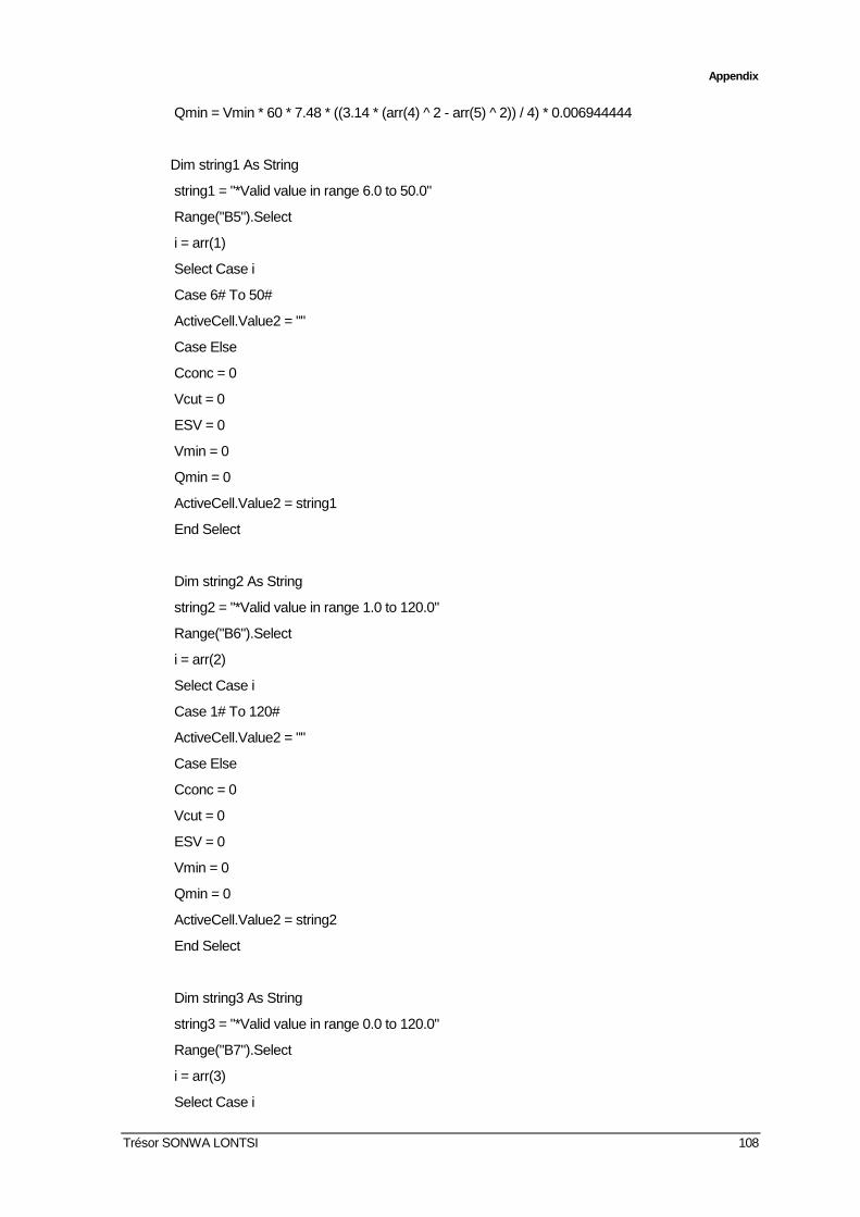
Appendix
Trésor SONWA LONTSI 108
Qmin = Vmin * 60 * 7.48 * ((3.14 * (arr(4) ^ 2 - arr(5) ^ 2)) / 4) * 0.006944444
Dim string1 As String
string1 = "*Valid value in range 6.0 to 50.0"
Range("B5").Select
i = arr(1)
Select Case i
Case 6# To 50#
ActiveCell.Value2 = ""
Case Else
Cconc = 0
Vcut = 0
ESV = 0
Vmin = 0
Qmin = 0
ActiveCell.Value2 = string1
End Select
Dim string2 As String
string2 = "*Valid value in range 1.0 to 120.0"
Range("B6").Select
i = arr(2)
Select Case i
Case 1# To 120#
ActiveCell.Value2 = ""
Case Else
Cconc = 0
Vcut = 0
ESV = 0
Vmin = 0
Qmin = 0
ActiveCell.Value2 = string2
End Select
Dim string3 As String
string3 = "*Valid value in range 0.0 to 120.0"
Range("B7").Select
i = arr(3)
Select Case i

Appendix
Trésor SONWA LONTSI 109
Case 0# To 120#
ActiveCell.Value2 = ""
Case Else
Cconc = 0
Vcut = 0
ESV = 0
Vmin = 0
Qmin = 0
ActiveCell.Value2 = string3
End Select
Dim string4 As String
string4 = "*Valid value in range 2.0 to 36.0"
Range("B8").Select
i = arr(4)
Select Case i
Case 2# To 36#
ActiveCell.Value2 = ""
Case Else
Cconc = 0
Vcut = 0
ESV = 0
Vmin = 0
Qmin = 0
ActiveCell.Value2 = string4
End Select
Dim string5 As String
string5 = "*Valid value in range 1.0 to 30.0"
Range("B9").Select
i = arr(5)
Select Case i
Case 1# To 30#
ActiveCell.Value2 = ""
Case Else
Cconc = 0
Vcut = 0
ESV = 0
Vmin = 0
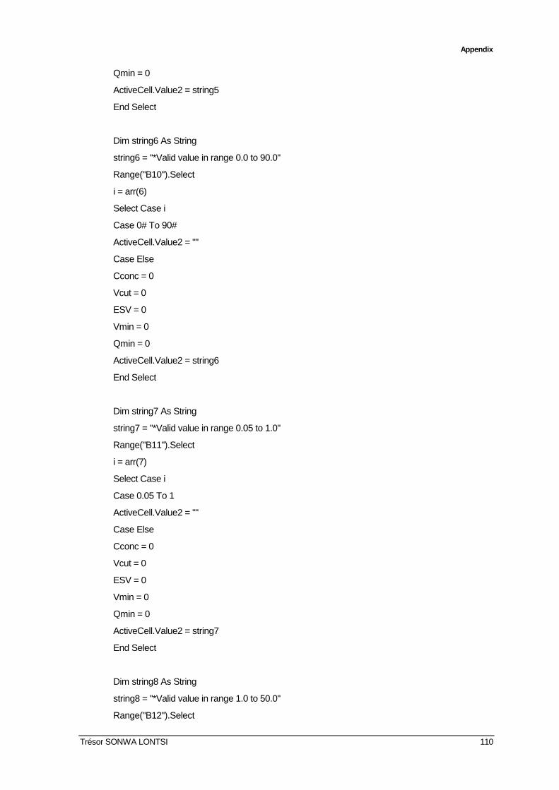
Appendix
Trésor SONWA LONTSI 110
Qmin = 0
ActiveCell.Value2 = string5
End Select
Dim string6 As String
string6 = "*Valid value in range 0.0 to 90.0"
Range("B10").Select
i = arr(6)
Select Case i
Case 0# To 90#
ActiveCell.Value2 = ""
Case Else
Cconc = 0
Vcut = 0
ESV = 0
Vmin = 0
Qmin = 0
ActiveCell.Value2 = string6
End Select
Dim string7 As String
string7 = "*Valid value in range 0.05 to 1.0"
Range("B11").Select
i = arr(7)
Select Case i
Case 0.05 To 1
ActiveCell.Value2 = ""
Case Else
Cconc = 0
Vcut = 0
ESV = 0
Vmin = 0
Qmin = 0
ActiveCell.Value2 = string7
End Select
Dim string8 As String
string8 = "*Valid value in range 1.0 to 50.0"
Range("B12").Select

Appendix
Trésor SONWA LONTSI 111
i = arr(8)
Select Case i
Case 1# To 50#
ActiveCell.Value2 = ""
Case Else
Cconc = 0
Vcut = 0
ESV = 0
Vmin = 0
Qmin = 0
ActiveCell.Value2 = string8
End Select
Dim string11 As String
string11 = "*Valid value in range 10.0 to 3000.0"
Range("B15").Select
i = arr(11)
Select Case i
Case 10# To 3000#
ActiveCell.Value2 = ""
Case Else
Cconc = 0
Vcut = 0
ESV = 0
Vmin = 0
Qmin = 0
ActiveCell.Value2 = string11
'MsgBox ActiveCell.Value2
'ActiveCell.Value = " * Please enter a value between 0.05 and 1"
'MsgBox "Valid value for the diameter of particle in range 0.05 to 1 ", vbExclamation
End Select
Range("B26").Select
ActiveCell.Value = Cconc
Range("B30").Select
ActiveCell.Value = Vcut
Range("B31").Select
ActiveCell.Value = ESV

Appendix
Trésor SONWA LONTSI 112
Range("B32").Select
ActiveCell.Value = Vmin
Range("B33").Select
ActiveCell.Value = Qmin
End Sub
Private Sub CommandButton2_Click()
Range("B5").Select
TextBox1.Value = ""
TextBox2.Value = ""
TextBox3.Value = ""
TextBox4.Value = ""
TextBox5.Value = ""
TextBox6.Value = ""
TextBox7.Value = ""
TextBox8.Value = ""
TextBox9.Value = ""
TextBox10.Value = ""
TextBox11.Value = ""
TextBox12.Value = ""
'ActiveCell.Offset(1, 0).Select
End Sub
10.2 Appendix B
10.2.1 Minimum transport velocity (MTV) calculation6
The calculation of the Minimum transport velocity and the minimum flow rate to keep the
well clean, very complexes calculations must be done. Using the Larsen method developed
in this work and with the given drilling parameters, the critical flow rate and cuttings bed
concentration can be highlighted.

Appendix
Trésor SONWA LONTSI 113
DRILLING PARAMETERS FOR CALCULATIONS
Drilling fluid polymer mud Yield point lbf/sqft 7 Plastic viscosity cp 7 Pump operating flow rate gal/min 600 Angle of inclination degree 47 Cuttings size inches 0,175 Mud weight lbm/gal 11,1 Rate of penetration ft/hr 52 Hole diameter inches 12,25 Pipe diameter inches 5,5 Bed porosity % 36
To calculate in this example is the minimum flow velocity, flow rate to transport all the
cuttings to the surface, and the cuttings concentration at the operating flow rate of 600
gal/min.
Minimum Flow rate prediction:
Cuttings concentration at the minimum flow rate can be calculated with the equation 26.
concC = 0, 01902 x 52 + 0, 495 = 1, 48%
Average cuttings transport at the minimum flow rate:
48,125,12
5,5136
522
×
−
=cutV = 1, 22 ft/sec
Equivalent slip velocity calculation (ESV): to find the ESV, the apparent viscosity aµ has
to be calculated. The apparent viscosity will be calculated by estimating the minimum
transport velocity to clean up the hole minV and iterating until an acceptable value has been
obtained. First the ESV has to be estimated, as for example 3, 3 ft/sec. This will lead to:
sec/52,4sec/3,3sec/22,1min ftftftV estimated =+=−
Than the apparent viscosity can be calculated using the equation 31:
( )52,4
5,525,12757
−××+=aµ = 59, 3 cp
As aµ > 55 cp, ESV will be calculated with the equation 30:

Appendix
Trésor SONWA LONTSI 114
26,33,59025,0 +×=ESV = 4, 74 ft/sec
For a better accuracy, the calculated ESV will be used for a calculation of new minV and a
new aµ which lead to:
sec/96,5sec/74,4sec/22,1min ftftftV calc =+=−
Based on this calcV −min the new apparent viscosity is calculated, newaµ by the same equation
31 as:
( )96,5
5,525,12757
−××+=−newaµ = 46, 64 cp
And the newESV have to be calculated by the equation 30 as:
10,364,460052,0 +×=newESV = 3, 34 ft/sec
This iteration has to be done till:
01,0≤− ESVESVabs new
For the simplicity of the example let us assume that sec/34,32 ftESVnew = . The correction of
the angle, cuttings size and mud weight must been taking into consideration.
Angle of inclination correction factor: Using the equation 32,
08,120,0470002,0470365,0 2 =−×−×=angC
Cuttings size correction factor: Using the equation 33:
09,127,1175,002,1 =+×−=sizeC
Mud weight correction factor: Using the equation 35:
1=MWC
The cuttings slip velocity can be now found with the equation 36 by:
sec/93,3109,108,134,3 ftVslip =×××=
The minimum transport velocity can be calculated by the equation 37.
sec/15,5sec/93,3sec/22,1min ftftftV =+=

Appendix
Trésor SONWA LONTSI 115
And the corresponding apparent viscosity is about cpenda 8,43=−µ
The minimum transport velocity must be converted into flow rate in order to compare with
the operating flow rate 600 gal/min.
annAft
galftQ ×
=3min 1
48,7
min1
sec60
sec15,5
The cross sectional area of the annulus can be calculated by:
( )4
22pipehole
ann
DDA
−=
π
( ) 2222
68,02,984
5,525,1214,3ftin ==−×=
min/1576min galQ = . As minimum flow rate is higher than the operating flow rate the
cuttings will accumulate in the borehole. The cuttings accumulation can be calculated by:
( )Φ−
−= 11
minQ
QC pump
cutt
( ) %3939,036,011576
6001 ==−
−=
Correction for cuttings accumulation:
87,08,4300231,097,0 =×−=−cuttCFC
The corrected cuttings accumulation is calculated by:
cuttCFcuttcutt CCC −×=
%3438,087,039,0 ==×=