Masses, Radii, and Orbits of SmallKepler Planets: The TransitionFrom Gaseous to Rocky Planets

The Harvard community has made thisarticle openly available. Please share howthis access benefits you. Your story matters

Citation Marcy, Geoffrey W., Howard Isaacson, Andrew W. Howard,Jason F. Rowe, Jon M. Jenkins, Stephen T. Bryson, David W.Latham, et al. 2014. Masses, Radii, and Orbits of Small KeplerPlanets: The Transition From Gaseous to Rocky Planets.The Astrophysical Journal Supplement Series 210, no. 2: 20.doi:10.1088/0067-0049/210/2/20.

Published Version doi:10.1088/0067-0049/210/2/20

Citable link http://nrs.harvard.edu/urn-3:HUL.InstRepos:29990226

Terms of Use This article was downloaded from Harvard University’s DASHrepository, and is made available under the terms and conditionsapplicable to Open Access Policy Articles, as set forth at http://nrs.harvard.edu/urn-3:HUL.InstRepos:dash.current.terms-of-use#OAP

arX

iv:1

401.

4195

v1 [

astr

o-ph

.EP]

16

Jan

2014

Accepted by ApJSPreprint typeset using LATEX style emulateapj v. 04/17/13

MASSES, RADII, AND ORBITS OF SMALL KEPLER PLANETS:THE TRANSITION FROM GASEOUS TO ROCKY PLANETS †

Geoffrey W. Marcy1 , Howard Isaacson1, Andrew W. Howard29, Jason F. Rowe2, Jon M. Jenkins3,Stephen T. Bryson2, David W. Latham8, Steve B. Howell2, Thomas N. Gautier III6, Natalie M. Batalha2,

Leslie A. Rogers22, David Ciardi14, Debra A. Fischer19, Ronald L. Gilliland10, Hans Kjeldsen12,Jørgen Christensen-Dalsgaard12,13, Daniel Huber2, William J. Chaplin41,12 Sarbani Basu19 Lars A. Buchhave8,55,Samuel N. Quinn8, William J. Borucki2, David G. Koch2, Roger Hunter2, Douglas A. Caldwell3, Jeffrey Van

Cleve3, Rea Kolbl1, Lauren M. Weiss1, Erik Petigura1, Sara Seager16, Timothy Morton22,John Asher Johnson22, Sarah Ballard30, Chris Burke3, William D. Cochran7, Michael Endl 7, Phillip

MacQueen 7, Mark E. Everett35, Jack J. Lissauer2, Eric B. Ford20, Guillermo Torres8, Francois Fressin8,Timothy M. Brown9, Jason H. Steffen17, David Charbonneau8, Gibor S. Basri1, Dimitar D. Sasselov8, Joshua

Winn16 Roberto Sanchis-Ojeda16 Jessie Christiansen2, Elisabeth Adams47, Christopher Henze2,Andrea Dupree8, Daniel C. Fabrycky54, Jonathan J. Fortney18, Jill Tarter3, Matthew J. Holman8,

Peter Tenenbaum3, Avi Shporer22, Philip W. Lucas24, William F. Welsh25, Jerome A. Orosz25, T. R. Bedding48,T. L. Campante41,12, G. R. Davies41,12, Y. Elsworth41,12, R. Handberg41,12, S. Hekker49,50, C. Karoff12,

S. D. Kawaler51, M. N. Lund12, M. Lundkvist12, T. S. Metcalfe52, A. Miglio41,12 V. Silva Aguirre12, D. Stello48,T. R. White48 Alan Boss26, Edna Devore3, Alan Gould27, Andrej Prsa28, Eric Agol30, Thomas Barclay31, JeffCoughlin31, Erik Brugamyer33, Fergal Mullally3, Elisa V. Quintana3, Martin Still31, Susan E. Thompson3,

David Morrison2, Joseph D. Twicken3, Jean-Michel Desert8, Josh Carter16, Justin R. Crepp34,Guillaume Hebrard42,43, Alexandre Santerne44,45, Claire Moutou53, Charlie Sobeck2, Douglas Hudgins46,

Michael R. Haas2, Paul Robertson20,7 Jorge Lillo-Box56, David Barrado56

Accepted by ApJS

ABSTRACT

We report on the masses, sizes, and orbits of the planets orbiting 22 Kepler stars. There are 49planet candidates around these stars, including 42 detected through transits and 7 revealed by preciseDoppler measurements of the host stars. Based on an analysis of the Kepler brightness measurements,along with high-resolution imaging and spectroscopy, Doppler spectroscopy, and (for 11 stars) astero-seismology, we establish low false-positive probabilities for all of the transiting planets (41 of 42 havea false-positive probability under 1%), and we constrain their sizes and masses. Most of the transit-ing planets are smaller than 3× the size of Earth. For 16 planets, the Doppler signal was securelydetected, providing a direct measurement of the planet’s mass. For the other 26 planets we provideeither marginal mass measurements or upper limits to their masses and densities; in many cases wecan rule out a rocky composition. We identify 6 planets with densities above 5 g cm−3, suggestinga mostly rocky interior for them. Indeed, the only planets that are compatible with a purely rockycomposition are smaller than ∼2 R⊕. Larger planets evidently contain a larger fraction of low-densitymaterial (H, He, and H2O).

Keywords: planetary systems — stars: individual (Kepler) — techniques: photometry, radial velocity

1 University of California, Berkeley, CA 947202 NASA Ames Research Center, Moffett Field, CA 940353 SETI Institute/NASA Ames Research Center, Moffett Field,

CA 940354 San Jose State University, San Jose, CA 951925 Lowell Observatory, Flagstaff, AZ 860016 Jet Propulsion Laboratory/Caltech, Pasadena, CA 911097 University of Texas, Austin, TX 787128 Harvard Smithsonian Center for Astrophysics, 60 Garden

Street, Cambridge, MA 021389 Las Cumbres Observatory Global Telescope, Goleta, CA 9311710 Center for Exoplanets and Habitable Worlds, The Pennsylva-

nia State University, University Park, 1680211 Niels Bohr Institute, Copenhagen University, Denmark12 Stellar Astrophysics Centre (SAC), Department of Physics

and Astronomy, Aarhus University, Ny Munkegade 120, DK-8000Aarhus C, Denmark

13 High Altitude Observatory, National Center for AtmosphericResearch, Boulder, CO 80307

14 NASA Exoplanet Science Institute/Caltech, Pasadena, CA91125

15 National Optical Astronomy Observatory, Tucson, AZ 8571916 Massachusetts Institute of Technology, Cambridge, MA,

0213917 Northwestern University, Evanston, IL, 60208, USA

18 University of California, Santa Cruz, CA 9506419 Yale University, New Haven, CT 0651020 Center for Exoplanets and Habitable Worlds, Department

of Astronomy and Astrophysics, 525 Davey Laboratory, ThePennsylvania State University, University Park, PA, 16802, USA

21 Orbital Sciences Corp., NASA Ames Research Center,Moffett Field, CA 94035

22 California Institute of Technology, Pasadena, CA 9110923 Department of Physics, Broida Hall, University of California,

Santa Barbara, CA 9310624 Centre for Astrophysics Research, University of Hertfordshire,

College Lane, Hatfield, AL10 9AB, England25 San Diego State University, San Diego, CA 9218226 Carnegie Institution of Washington, Dept. of Terrestrial

Magnetism, Washington, DC 2001527 Lawrence Hall of Science, Berkeley, CA 9472028 Villanova University, Dept. of Astronomy and Astrophysics,

800 E Lancaster Ave, Villanova, PA 1908529 University of Hawaii, Honolulu, HI30 Department of Astronomy, Box 351580, University of Wash-

ington, Seattle, WA 98195, USA31 Bay Area Environmental Research Institute/ Moffett Field,

CA 94035, USA32 Vanderbilt University, Nashville, TN 37235, USA33 McDonald Observatory, University of Texas at Austin,

2 Marcy et al.

1. INTRODUCTION

Our Solar System contains no planets with radii be-tween Earth and Neptune (3.9 R⊕), a size gap that dif-fers from the apparent distribution of small planets inthe Milky Way and requires adjustments to the core-accretion model to explain. For example, Uranus andNeptune, with equatorial radii of 4.01 and 3.88 R⊕, re-spectively, and their massive rocky cores would presum-ably have grown to Saturn or even Jupiter size throughrunaway accretion had the protoplanetary disk not disap-peared when it did (Pollack et al. 1996; Goldreich et al.2004; Rogers & Seager 2010b; Morbidelli 2013). Still,based on formation models of our own Solar System, thesize domain of 1–4 R⊕ was expected to be nearly de-serted (Ida & Lin 2010; Mordasini et al. 2012). It is not.Instead, most of the observed planets around other starshave radii in the range of 1–4 R⊕ (Borucki et al. 2011;Batalha et al. 2013).This great population of sub-Neptune-size exoplanets

had first been revealed by precise Doppler surveys ofsolar-mass stars within 50 pc. Such surveys find planetcounts increase toward smaller masses, at least within therange of 1000 M⊕ down to ∼5 M⊕ (Howard et al. 2010;Mayor et al. 2011). Independently, the NASA Keplertelescope finds that 85% of its transiting planet “can-

Austin, TX, 78712, USA34 University of Notre Dame, Notre Dame, Indiana 4655635 NOAO, Tucson, AZ 85719 USA36 Southern Connecticut State University, New Haven, CT

06515 USA37 MSFC, Huntsville, AL 35805 USA39 Las Cumbres Observatory Global Telescope, Goleta, CA

93117, USA40 Max Planck Institute of Astronomy, Koenigstuhl 17, 69115

Heidelberg, Germany41 School of Physics and Astronomy, University of Birmingham,

Edgbastron, Birmingham B15 2TT, UK42 Institut d’Astrophysique de Paris, UMR7095 CNRS, Univer-

site Pierre & Marie Curie, 98bis boulevard Arago, 75014 Paris,France

43 Observatoire de Haute Provence, CNRS/OAMP,04870 Saint-Michel-l’Observatoire, France

44 Aix Marseille Universite, CNRS, LAM UMR 7326, 13388,Marseille, France

45 Centro de Astrofisica, Universidade do Porto, Rua dasEstrelas, 4150-762 Porto, Portugal

46 NASA Headquarters, Washginton DC47 Planetary Science Institute, 1700 East Fort Lowell, Suite 106,

Tucson, AZ 8571948 Sydney Institute for Astronomy, School of Physics, University

of Sydney 2006, Australia49 Max-Planck-Institut fur Sonnensystemforschung, 37191

Katlenburg-Lindau, Germany50 Astronomical Institute, “Anton Pannekoek”, University of

Amsterdam, The Netherlands51 Department of Physics and Astronomy, Iowa State University,

Ames, IA, 50011, USA52 Space Science Institute, Boulder, CO 80301, USA53 Canada-France-Hawaii Telescope, 65-1238 Mamalahoa Hwy,

Kamuela, Hawaii, 96743, USA54 Department of Astronomy and Astrophysics, University of

Chicago, 5640 S.Ellis Ave., Chicago, IL 60637, USA55 Centre for Star and Planet Formation, Natural History

Museum of Denmark, University of Copenhagen, DK-1350 Copen-hagen, Denmark

56 Depto. Astrofısica, Centro de Astrobiologıa (INTA-CSIC),ESAC campus, P.O. Box 78, E-28691 Villanueva de la Canada,Spain

† Based in part on observations obtained at the W. M. KeckObservatory, which is operated by the University of California andthe California Institute of Technology.

didates” have radii less than 4 R⊕ (Batalha et al. 2013).Since more than 80% of these small planet candidates areactually planets (Morton & Johnson 2011; Fressin et al.2013), the population of sub-4-R⊕ planets is assuredlylarge (but see Santerne et al. 2012 for the confirmationrate of Jupiter-size planets). No detection bias wouldfavor the discovery of small planets over the large ones(for a given orbital period), and indeed the small planetsenjoy a smaller rate of false-positive scenarios. Thus, inboth the solar vicinity probed by Doppler surveys andin the Kepler field of view (slightly above the plane ofthe Milky Way), an overwhelming majority of planetsorbiting within 1 au of solar-type stars are smaller thanUranus and Neptune (i.e., <∼4 R⊕).For planets orbiting close to their host star, the great

occurrence of small planets is particularly well deter-mined. Within 0.25 au of solar-type stars, the numberof planets rises rapidly moving from 15 R⊕ to 2 R⊕,based on analyses of Kepler data that correct for detec-tion biases due to photometric noise, orbital inclination,and the completeness of the Kepler planet-search de-tection pipeline (Howard et al. 2012; Fressin et al. 2013;Petigura et al. 2013). Further corrections for photomet-ric SNR and detection completeness show that the oc-currence of planets remains at a (high) constant level forsizes from 2 to 1 R⊕, with ∼15% of FGK stars havinga planet of 1–3 R⊕ within 0.25 au (Fressin et al. 2013;Petigura et al. 2013).With no Solar System analogs, the chemical com-

positions, interior structures, and formation pro-cesses for 1–4 R⊕ planets, including their gravita-tional interactions with other planets, present pro-found questions (Seager et al. 2007; Fortney et al. 2007;Zeng & Seager 2008; Rogers et al. 2011; Zeng & Sasselov2013; Lissauer et al. 2011, 2012; Fabrycky et al. 2012).Determining chemical composition is one step toward adeeper understanding, but at this planet-size scale, therelative amounts of rock, water, and H and He gas re-main poorly known. Most likely, the admixture of thosethree ingredients changes as a function of planet mass,but differs among planets at a given mass, as well.Beyond the question of their characteristics, these

1–4 R⊕ planets pose a great challenge for the the-ory of planet formation: like Venus, Earth, Uranus,and Neptune, they likely contain a ratio of rock tolight material that is much greater than cosmic abun-dances, and therefore their formation must have re-quired some complex processing in the protoplanetarydisk. However, new ideas are emerging about the for-mation of such Neptune-mass-and-smaller planets, mostof which are variations on the theme of core-accretiontheory (Chiang & Laughlin 2013; Mordasini et al. 2012;Hansen & Murray 2013). Particularly intriguing is thenotion that taken as an ensemble, the hundreds of Ke-pler exoplanet candidates reflect the mass densities ofprotoplanetary disks during the period of planet forma-tion, leading to a theory that within 0.5 au of their hoststars, sub-Neptunes formed in situ, i.e., without migra-tion (Chiang & Laughlin 2013; Hansen & Murray 2013).The predicted relations between mass, radius, and inci-dent flux agree with those observed (Lopez et al. 2012;Lopez & Fortney 2013; Weiss et al. 2013). These modelsand their associated predictions of in situ mini-Neptuneand super-Earth formation can be further tested with

Kepler Planet Masses 3

accurate measurements of planet masses and radii.Measuring masses for transiting planets that already

have measured radii can constrain the mean molecularweight, internal chemical composition, and hence forma-tion mechanisms for 1–4 R⊕ planets (Seager et al. 2007;Zeng & Seager 2008; Zeng & Sasselov 2013; Rogers et al.2011; Chiang & Laughlin 2013). Only a handful of smallplanets have mass measurements, and those with radiiabove 2 R⊕ often have low densities inconsistent withpure rocky composition. Two well-studied examples areGJ 436 b and GJ 1214 b (Maness et al. 2007; Gillon et al.2007; Torres et al. 2008; Charbonneau et al. 2009) withradii of 4.21 and 2.68 R⊕, masses of 23.2 and 6.55 M⊕,and resulting bulk densities of 1.69 and 1.87 g cm−3, re-spectively. Their densities are slightly higher than thoseof Uranus and Neptune (1.27 and 1.63 g cm−3), butstill well below Earth’s (5.5 g cm−3). The sub-Earthbulk densities indicate that the two exoplanets con-tain significant amounts of low-density material (by vol-ume), presumably H, He, and water (Figueira et al. 2009;Rogers & Seager 2010a; Batygin & Stevenson 2013). Atthe larger end of the small-planet spectrum is Kepler-18c, with a radius of 5.5R⊕ but a mass of only 17.3M⊕, im-plying a low density of 0.59 ± 0.07 g cm−3(Cochran et al.2011). Similarly, HAT-P-26, with 6.3 R⊕, has low den-sity of 0.40 ± 0.1 g cm−3(Hartman et al. 2011).The several other ∼2–4 R⊕ exoplanets with se-

cure masses and radii support this trend, includingthe five inner planets around Kepler-11, GJ 3470b, 55 Cnc e, and Kepler-68 b (Lissauer et al. 2013;Bonfils et al. 2012; Endl et al. 2012; Demory et al. 2013,2011; Gilliland et al. 2013). All of these planets havedensities less than 5 g cm−3and some under 1 g cm−3,indicating a significant amount of light material by vol-ume (H, He, water) mixed with some rock and Fe. (Theuncertainties for 55 Cnc e admit the possibility this 2.1R⊕ planet could be pure rock.) Perhaps these securelymeasured lower-than-rock densities are representative ofplanets of size 2.0—4.5 R⊕ in general, and hence repre-sentative of the chemical composition of such planets.Most tellingly, the five planets with radii less

2 R⊕, namely CoRoT 7b, Kepler-10b, Kepler-36b, KOI-1843.03, and Kepler-78b all have mea-sured densities of 6–10 g cm−3(Queloz et al. 2009;Batalha et al. 2011; Carter et al. 2012; Rappaport et al.2013; Sanchis-Ojeda et al. 2013; Pepe et al. 2013;Howard et al. 2013). Thus, below 2 R⊕ some planetshave densities consistent with pure solid rock andiron-nickel. The dichotomy of planet densities hasbeen considered theoretically as due to accumulationand photo-evaporation of volatiles (Chiang & Laughlin2013; Hansen & Murray 2013; Lopez et al. 2012;Lopez & Fortney 2013).To quantify this transition to rocky planets, one may

use the extant empirical relation between density andplanet mass that has been discovered for the planetssmaller than 5 R⊕: ρ = 1.3M−0.60

p F−0.09, where ρ is

in g cm−3, Mp is in M⊕, and F is the incident stellarflux on the planet in erg s−1 cm−2 (Weiss et al. 2013).The Weiss et al. relation shows that planets with massesover ∼2 M⊕ (equivalently, with radii over 1.5 R⊕) havetypical densities less than 5.5 g cm−3and hence typicallycontain significant amounts of light material (H, He, and

water). Thus, the transition from planets containing sig-nificant light material to those that are rocky occurs atplanet radii near 1.0–2.5 R⊕, i.e., masses near 1–3 M⊕ ,based tentatively on the handful of planets in that sizedomain located within 0.2 au. This suggestion of a tran-sition to rocky planets below masses of 3 M⊕ is a majorresult from current Kepler exoplanet observations.However, the Weiss et al. relation, and the predicted

transition to rocky planets below 2 R⊕, is based on themeasured masses and radii of only a handful of planets.It surely requires both confirmation and quantification,by measuring the masses and radii of more small exoplan-ets. Those additional small exoplanets would also greatlyinform models of planet formation, based on correlationsbetween the volatile or rocky nature of the planets andthe metallicities of their host stars (Buchhave et al. 2012;Latham & Buchhave 2012; Johnson et al. 2007).Here we report measured masses, radii, and densities

(or upper limits on those values) for 42 transiting planetcandidates contained within 22 bright Kepler Objectsof Interest (KOIs) from Batalha et al. (2013). We car-ried out multiple Doppler-shift measurements of the hoststars using the Keck 1 telescope. From the spectroscopyand Doppler measurements, we compute self-consistentmeasurements of stellar and planet radii, employing ei-ther stellar structure models or asteroseismology mea-surements from the Kepler photometry. We also searchfor (and report) 7 additional non-transiting planets re-vealed by the precise radial velocities, for a total of 49planets.

2. VETTING AND SELECTION OF 22 TARGET KOIS

This paper contains the results of extensive precise-RV measurements of KOIs, made by the Kepler team.The intense RV follow-up observations described herewere carried out on 22 KOIs chosen through a care-ful vetting process. The initial identification of theKOIs from the photometry was an extensive, itera-tive program carried out by the Kepler team duringthe nominal NASA mission from launch 2009 Marchto 2012 November. The identification process hasbeen described elsewhere, notably by Caldwell et al.(2010); Jenkins et al. (2010b,a); Van Cleve & Caldwell(2009), and Argabright et al. (2008), with an overviewin Borucki et al. (2010). The ∼2300 KOIs identified inthese searches are listed in Batalha et al. (2013).

2.1. Data Validation: TCERT

The selection of the 22 KOIs for this study involvedseveral major stages of pruning of the candidates, start-ing with the “threshold crossing events” (TCEs) thatare the series of repeated dimmings found for a partic-ular star by the Kepler “Transit Planet Search” (TPS)pipeline. Working within the Kepler TCE review team(“TCERT”), we vetted the TCEs to distinguish planetcandidates from false positives and to measure more ac-curately the properties of the planets and their host stars.Detailed descriptions of the components of this TCE vet-ting can be found in Gautier et al. (2010); Borucki et al.(2011); Batalha et al. (2013).A TCE was elevated to KOI status (planet candidate)

based on simple (often eye-ball) criteria involving theinspection of each Kepler light curve, using long ca-dence photometry, overplotted on a model of a transiting

4 Marcy et al.

planet, and noting a lack of eclipsing binary signaturessuch as secondary eclipses and “odd-even” alternate vari-ability of successive transit depths. This TCERT-basedidentification of the KOIs involved only Kepler data, notoutside observations.Actual transiting planets should exhibit photometry

that is well fit, within errors, by a transiting planetmodel. They should also show an astrometric displace-ment (if any) during transit that is consistent with thehypothesis that the intended target star is the sourceof the photometric variations during transit. Such“Data Validation” (DV) techniques are described inBatalha et al. (2010, 2011); Bryson et al. (2013). TheseDV tests have undergone improvements and automationduring the past three years (Wu et al. 2010; Bryson et al.2013). All 22 KOIs in this work passed their DV tests,conferring KOI status on them as continued planet can-didates. Details on the nature of DV criteria for eachKOI are given below in Section 7.The TCERT identification of KOIs as “planet candi-

dates” made them worthy of follow-up observations withother telescopes, designed both to weed out false posi-tives and to better measure the planet properties throughsuperior knowledge of host star properties, notably radii.Various types of follow-up observations of some, but notall, of the ∼2300 KOIs had been carried out by the timeof our selection process of the 22 KOIs studied here. Pub-lication of those KOIs are in Borucki et al. (2011, 2012);Batalha et al. (2013).

2.2. Follow-Up Observation Program: KFOP

We activated in May 2009 the Kepler “Follow-up Ob-servation Program” (KFOP) with the goals of vetting theKOIs for false positives and improving the measurementof the planet radii. The goals were to characterize allof the KOIs, as resources permitted, using a variety ofground-based telescopes. Each of the KOIs first had theirKepler light curves and astrometric integrity scrutinizedagain, polishing the TCERT vetting. Here we summarizethe key KFOP observational efforts that were carried outon ∼1000 KOIs from which the 22 KOIs presented herewere selected.In brief, each of the ∼1000 KOIs had its light curve fur-

ther scrutinized and its position further measured (Sec-tion 2.1) to alert us to angularly nearby stars (within2′′) in the photometric aperture. As described below,we carried out adaptive optics (AO) imaging and speckleinterferometry (Section 2.2.3 and Section 2.2.2) to huntfor neighboring stars. KOIs having a neighboring starwithin 2′′ and brighter than 1% of the primary star arenot amenable for follow-up spectroscopy due to the lightfrom both stars entering the slit. Roughly 20% of theKOIs were deemed not suitable for spectroscopy due aclose stellar neighbor.KOIs meeting those criteria were observed with high-

resolution, low-SNR echelle spectroscopy to measure at-mospheric stellar parameters, magnetic activity, and ro-tational Doppler broadening, designed to detect bina-ries and, importantly, to assess suitability for precise RVmeasurements. Only single, FGKM-type stars with nar-row lines (v sin i< 10 kms−1 ) are suitable for the highestprecision RV measurements. Below is a summary of thenature of these KFOP vetting actions on over 1000 KOIs,prioritized by brightness, leading to the selection of the

22 KOIs in this study. KOIs brighter than Kp∼14.5mag received most of the KFOP observational resources,while those fainter than Kp=15 mag were only rarelyobserved.

2.2.1. Follow-Up Reconnaissance Spectroscopy

We carried out “reconnaissance” high-resolution spec-troscopy on ∼1000 KOIs with spectral resolution,R∼50,000, and SNR = 20−100 per pixel. The dual goalswere searching for false positives and refining the stellarparameters. We obtained one or two such reconnaissancespectra using one of four facilities: the McDonald Obser-vatory 2.7 m, the Tillinghast 1.5 m on Mt. Hopkins,the Lick Observatory 3 m, and the 2.6-m Nordic OpticalTelescope.Of greatest importance was to detect angularly nearby

stars that, themselves, might be eclipsed or transited bya companion star or planet, the light from which wouldbe diluted by the primary star mimicking a transitingplanet around it. With a typical spectrometer slit widthof 1′′, stellar companions within 0.′′5 would send light intothe slit, permitting their detection if bright enough (seebelow). A cross correlation of each spectrum was per-formed, usually with a best-matched synthetic template,to detect stellar companions separated by more than ∼10kms−1 in radial velocity and brighter than ∼5% of theprimary in optical flux.Also, a second reconnaissance spectrum was obtained

to detect radial velocity (“RV”) variation above a thresh-old of ∼0.5 km s−1 , indicating the presence of a binary.We selected the 22 KOIs in this paper by rejecting allKOIs that showed such RV variation from binary mo-tion. The fraction of KOIs rejected by reconnaissancespectroscopy was roughly 5%, leaving 95% as survivingplanet candidates. The absence of a secondary spectrumand RV variations (confirmed later by the precise RVswith 2 m s−1 precision) for all 22 KOIs rules out a largeportion of parameter space for possible false positives inthe form of an angularly nearby star that may be thesource of the periodic dimming. As described in Section6, a further analysis of the Keck-HIRES spectra takenlater with high SNR further ruled out stellar companionswithin 0.′′5 down to optical flux levels of 1% that of theprimary star.The reconnaissance spectra were also analyzed to mea-

sure the properties of the host star more precisely thanwas available in the Kepler Input Catalog (KIC). Thespectra were analyzed by comparing each one to a libraryof theoretical stellar spectra, e.g., Buchhave et al. (2012).This “recon” analysis (later refined by Buchhave et al. as“SPC” analysis) was done with grid step sizes between in-dividual library spectra of 250 K for Teff , 0.5 dex for log g,1 kms−1 for v sin i, and 0.5 dex in metallicity ([m/H]).This “recon” spectroscopy analysis yielded approximatevalues of Teff (within 200 K), log g (within 0.10 dex),and v sin i (within 2 kms−1 ) for the primary star of theKOI, valuable for deciding whether the KOI was suit-able for follow-up precise RV observations. Only starscooler than 6100 K on the main sequence (log g> 4.0)with v sin i< 5 km s−1 were deemed suitable for the RVmeasurements of highest precision near ∼2 m s−1 . Allrelevant details about the reconnaissance spectroscopyfor each KOI are given in Section 7.

Kepler Planet Masses 5

2.2.2. Speckle Imaging

Speckle imaging of each of the 22 KOIs was obtainedusing the two-color DSSI speckle camera at the WIYN3.5 m telescope on Kitt Peak, with technical detailsgiven in Howell et al. (2011); Horch et al. (2009). Thespeckle camera simultaneously obtained 3,000 images of40 msec duration in two filters: V (5620/400A) and R(6920/400A). These data yielded a final speckle image foreach filter. Section 7 describes the results of the speckleobservation for each KOI noting if any other sources ap-peared.The speckle data for each star allowed detection of a

companion star within the 2.′′76× 2.′′76 field of view cen-tered on the target. The speckle observations could de-tect, or rule out, companions between 0.′′05 and 1.′′5 fromeach KOI. The speckle images were all obtained with theWIYN telescope during seeing of 0.′′6–1.′′0 . The thresh-old for detection of companion stars was a delta magni-tude of 3.8 mag in the R band and 4.1 mag in V band(within the sensitivity annulus from 0.′′05–1.′′5), relativeto the brightness of the KOI target star. For Kepler-97 the detection threshold was compromised by a stellarcompanion 0.′′36 away from the primary and 2.7 magni-tudes fainter at optical wavelengths (3.2 mag fainter inK band). This companion is farther than the maximumpossible separation of a false positive star, based on cen-troid astrometry in and out of transit.These speckle observations were used to select the 22

KOIs studied here, by rejecting all KOIs (roughly 5%)that showed such a stellar companion. Thus, these ini-tial speckle observations showed that none of the 22 KOIs(except Kepler-97) in this work had a detected compan-ion by speckle. This selection process using speckle imag-ing by which the 22 KOIs were chosen surely favors singlestars rather than binaries or multiples. Hence it elimi-nates, a priori, a major domain of false positives (i.e.neighboring stars with transiting companions).

2.2.3. AO Imaging

Near-infrared adaptive optics (AO) imaging was ob-tained for ∼300 KOIs of the 1000 KOIs brighter thanKp=14 mag. The goal, as with the speckle observa-tions described above, was to detect stellar companionsthat might be the source of the periodic dimming (a falsepositive). Seeing-limited imaging, obtained with varioustelescopes at both optical and IR wavelengths, revealedcompanions located more than 2′′ from the primary KOIstar. Seeing-limited J-band Images from UKIRT wereparticularly useful (Lawrence et al. 2007). (After selec-tion of the 22 KOIs here, we also examined optical seeing-limited images from the Keck-HIRES guide camera, andwe provide those images here.) Any seeing-limited im-ages showing a companion stars within 2′′ was rejectedas a useful candidate for high precision RV work, i.e. re-jected for inclusion in this study. Thus all 22 KOIs inthis paper were selected with a prior AO image, as wellas the speckle imaging described above.The strength of AO imaging is the ability to detect

companions located between 0.′′05–2.′′0 of the KOI pri-mary star with detection limits 6 - 8 magnitudes fainterthan the primary (depending on the telescope and AOcamera). The goal was to detect angularly nearby stars,either background or gravitationally bound, that might

potentially have an eclipsing companion or a transitingplanet that might mimic a transiting planet around theprimary star, i.e., a false positive.Four different AO instruments were used in the near IR

on four different telescopes, namely the Keck 2 telescopeon Mauna Kea (NIRC2-AO), the MMT telescope on Mt.Hopkins (ARIES), the 5m telescope on Mt. Palomar(PHARO), and the 3m telescope at Lick Observatory(IRCAL), each described briefly below (Hayward et al.2001; Troy & Chanan 2003; Adams et al. 2012). Afterthe 22 KOIs were selected based on an absence of stellarcompanions found with the reconnaissance AO observa-tions with those four AO instruments, we carried outsubsequent AO imaging with the Keck 2 telescope andNIRC2 camera, generally superior to the other imaging.All 22 KOIs were observed with the Keck NIRC2-AO

system (Wizinowich et al. 2004; Johansson et al. 2008).We employed a natural guide star rather than the laserguide star as the Galactic field is rich with useful 13thmag guide stars in the Kepler field. We obtained all im-ages on two nights, 2013 June 13/14 and 14/15. We usedthe K ′ filter (wavelength coverage 1.9–2.3 µ), except forthe brightest five KOIs for which we employed a narrow-band Bracket-gamma filter to avoid saturation and toachieve flatter wavefronts. On both nights the naturalseeing (before AO) was ∼0.′′2 (FWHM) in K ′-band.For each KOI, we obtained 15 images with NIRC2-AO,

employing a pattern of three dither positions (using thethree best quadrants on the detector) and 5 exposuresat each position. The images were sky-subtracted, flat-fielded, and co-added to yield a final AO image. All finalKeck AO images have a PSF with a FWHM of 0.′′05 ±

0.′′01, with a field of view of 2”.The detection thresholds from these Keck AO images

for each KOI are shown in Figures 1 - 44. The detectionthresholds uniformly yielded 5-sigma detection of delta-K ′-magnitude = 6 mag as close as 0.′′2 from the KOI.At 0.′′4, the detection threshold is delta-K ′-magnitude= 8 mag. Excellent spatial resolution and sensitivitypermit the detection of a large fraction of the backgroundstars that could mimic a transiting planet. This spatialresolution also permits detection of a significant fractionof the widely separated bound stellar companions, giventhe typical distances (∼200 pc) to these magnitude 10–13solar-type stars, as described in Section 6. None of the22 KOIs showed a stellar companion within 1”, exceptfor Kepler-97, described below.The AO-vetting of the ∼2000 KOIs was done with

four smaller telescopes. The MMT ARIES cameraachieves near diffraction-limited imaging, with typicalPSF FWHM of 0.′′25 in the J-band and 0.′′14 in the Ksband, yielding Strehl ratios of 0.3 in Ks and 0.05 in Jband(Adams et al. 2012). While guiding on the primarystar, a set of 16 images, on a four-point dither patternwas acquired for each KOI. Full details and a descriptionof calibration and reduction of the images is describedby Adams et al. (2012)Some KOIs were vetted with the Palomar 5m

“PHARO” adaptive optics camera, observed in both theKs and J infrared bands using a 5-point dither patternwith integration times between 1.4 and 70 seconds, de-pending on the target brightness. The AO system usedthe primary star itself, not a laser, to guide and correctthe images, achieving a best resolution of 0.′′05 at J and

6 Marcy et al.

0.′′09 in the Ks band, with Strehl ratios of 0.10–0.15 in Jand 0.35–0.5 in Ks. Typical detection thresholds were 7mag at a separation of 0.′′5 and 9.3 mag at 1.′′0.The remaining KOIs were AO-vetted with the Lick

Observatory 3-m telescope and high-resolution camera,′′IRCAL′′. Observations were made in Natural GuideStar(NGS) mode, allowing the AO system to guide onthe target star. The Lick IRCAL AO system, built byClaire Max and James R. Graham, is described in detailat

astro.berkeley.edu/~jrg/ircal/spie/ircal.html

This mode of observing allows stars as faint as Kp= 13.5 to be observed. Detection limits down to adelta-J-magnitude of 6 mag, as close as 0.′′1 are typi-cally achieved. Background sky emission in the J-bandis typically 16.0 magnitudes per square arcsecond. TheK-band background sky emission at Lick Observatory is10.3 magnitudes per square arcsecond, making K-bandobserving difficult. Typically only J-band images weretaken at Lick Observatory. For details about the IRCALAO system, see

mtham.ucolick.org/techdocs/instruments/

Adams et al. (2012) provides an excellent description ofAO imaging of KOIs.The AO imaging described above with five telescopes

revealed a companion star within 6′′ of nine targets:Kepler-103, 95, 109, 48,113, 96, 131, 97, and 407.The following KOIs have no detected stellar companionwithin 6′′: Kepler-100, 93, 102, 94, 106, 25, 37, 68, 98,99, 406, 408, and 409. Of the nine KOIs with a detectedcompanion, only one, Kepler-97, has a companion within1′′. See Table 3 for details.None of the nine stars having stellar companions reside

angularly within the maximum exclusion radius foundfrom astrometry in and out of transit (see Section 6.2 andTable 3). Thus we find that none of the neighboring starscan arguably be causing the dimming as a false positive.For Kepler-97, the observed neighboring star resides 0.′′38away while the exclusion radius is 0.′′20, suggesting thatthe companion does not cause the apparent transit in thephotometry.Toward selection of the 22 KOIs in this study, any KOI

with a neighboring star located within 2′′ that had morethan 1% the flux of the primary star at optical wave-lengths was rejected as a suitable candidate for preciseRV measurements due to the contamination of light fromthat nearby star and due to the possible false positive. Ofthe 22 KOIs in this paper, only Kepler-97 has a compan-ion within 2′′, and it is less than 1% of the brightness ofthe primary star at optical wavelengths, as described inSection 7. The collection of imaging data and the asso-ciated search for companions, as well as the photometryand RV measurements, are found in Figures 1 - 44.

2.3. Selecting the 22 KOIs

In the last three years of the four-year Kepler mis-sion, the TCERT committee systematically shifted itsprioritization to select smaller-radii planets for precise-RV follow-up observations. Initially, the criteria had em-phasized verifying the planet nature of KOIs. The ef-fort had favored large planets with sizes above 4 R⊕ and

short-period orbits that might yield a detectable RV vari-ation in the host star, to check the existence of Keplertransiting planets. Detections of the RV signatures ofthe large planets around Kepler 4, 5, 6, 7, and 8 followedfrom this conservative prioritization. After the successesof the first six months of the Kepler mission, the criteriashifted toward verifying and measuring the masses of thesmaller planets, 2–5 R⊕, and of planets in multi-planetsystems, if they were likely to be detected with RVs. Re-sulting RV detections included Kepler 10, 18, 20, 22, 25,and 68 yielding constraints on the masses of the planets.During the second and third years of the 4-year Ke-

pler mission, i.e., 2010 and 2011, the TCERT prioritiza-tion shifted toward planets having smaller radii, below3 R⊕ and down to 1.0 R⊕. Obviously such small plan-ets are expected to have low masses, inducing small RVamplitudes in their host star. We carried out careful,optimized selection of suitable KOIs for RV work.One selection criterion was a brightness limit, Kp <

13.5 mag, to permit Poisson-limited signal-to-noise ra-tios near 100 per pixel within a 45 minute exposure withthe Keck-HIRES spectrometer. Such exposures yield aphoton-limited Doppler precision of 1.5 m s−1 . Anotherselection criteria was Teff < 6100 K (based on recon-naissance spectra) to promote numerous, narrow spec-tral lines that contribute Doppler information. Anothercriterion was small rotational Doppler broadening of thespectral lines, v sin i < 5 km s−1, based on reconnaissancespectra, to limit broadening of the lines that degradesDoppler precision.In the face of pervasive astrophysical “jitter” of ∼1

m s−1 for G and K dwarfs (Isaacson & Fischer 2010), theKepler TCERT committee selected KOIs for which anestimated planet mass might be sufficient to induce anRV amplitude greater than 1 m s−1 . To anticipate theRV amplitude, we used a nominal mass based on theplanet radius taken from the KIC, coupled with a roughestimate of planet density for that radius. The den-sity assumptions were simplistically based on the plan-ets in our solar system along with the few known smallexoplanets, notably GJ436b, GJ1214b, and Kepler-10b.We simply assumed a rocky constitution and density of∼5.5 g cm−3for planets smaller than 2 R⊕. We assumeddensities of 2 g cm−3for planets of 2–5 R⊕, and we as-sumed densities of 1 g cm−3for planets larger than 5 R⊕.These densities allowed the TCERT to choose planetsthat might meet the criteria above, including a prospec-tive RV amplitude above 1 m s−1 . The selection pro-cess was imperfect and biased as the assumed stellar pa-rameters and planet densities were only approximatelyknown and the target KOIs were selected based on RVdetectability.Here we report on the 22 KOIs selected by the pro-

cess described above, with a preference for small plan-ets suitable for detection and mass determination byprecise RV measurements. All 22 KOIs are identifiedin Batalha et al. (2013), but the follow-up observations,their analysis, asteroseismology, and the RVs have notbeen published to date, except for Kepler-68 for whichwe provide an update to its long-period, non-transitingplanet. This sample of 22 KOIs contains neither a ran-dom selection of KOIs nor a defined distribution of anyparameters. They were selected during the first threeyears of ever-evolving criteria, as described above.

Kepler Planet Masses 7

Importantly, the planet masses were unknown at thetime of target selection, except for estimates based onmeasured planet radii and guesses of density. Thus, foreach of the selected planet candidates, the subsequentlymeasured planet mass provides an unbiased sampling ofplanet masses for its particular planet radius. We couldnot have selected planet candidates biased toward highor low planet masses for a given planet radius, as we hadno such mass indicator.

3. STELLAR CHARACTERIZATION

For each of the 22 KOIs, we obtained an optical “tem-plate” spectrum using the Keck telescope and HIRESechelle spectrometer (Vogt et al. 1994) with no iodinegas in the light path. Each spectrum spanned wave-lengths from 3600–8000 A, with a spectral resolutionof R=60,000 and typical SNR per pixel of 100–200.These template spectra were analyzed with the standardLTE spectrum synthesis code, SME (Valenti & Piskunov1996; Valenti & Fischer 2005; Fischer & Valenti 2005) toyield values of Teff , log g, and [Fe/H] yielding formal un-certainties (of roughly 50 K, 0.1 dex, and 0.05 dex, re-spectively, with slight differences in precision due to SNRand spectral type). We augment the formal uncertain-ties to account for addition contributions to errors seenin 56 transiting planet hosts for which constraints onstellar properties stem from analysis of the light curves(Torres et al. 2012). We added dispersions in quadratureof σTeff

= 59K, σ[Fe/H] = 0.062 dex. Values of log g aresomewhat more uncertain and may be systematically inerror for Teff > 6100 K, due to poor sensitivity of themagnesium b triplet lines to surface gravity (Torres et al.2012).For 11 of the 22 KOIs an asteroseismic signal was de-

tected in the Kepler photometry, namely for Kepler-100, 93, 103, 95, 109, 25, 37, 68, 406, 408 and 409.For those 11 KOIs the output stellar parameters fromthe SME analysis Teff , log g, and [Fe/H], were fed intothe asteroseismology analysis as priors. The astero-seismology analysis yielded a more precise measure ofstellar radius and mass, and hence of surface gravity.This surface gravity was fed back, frozen, in the SMEanalysis of the spectrum, allowing a redetermination ofTeff and [Fe/H] without the usual covariances with log g.The resulting values of Teff and [Fe/H] were then fedback to an asteroseismology analysis as before, achiev-ing an iterative convergence quickly (Huber et al. 2013;Gilliland et al. 2013). The resulting uncertainties in stel-lar radius are between 2 and 4% (Huber et al. 2013).Stellar parameters for these 11 KOIs with asteroseismol-ogy are reported in Table 1.For the remaining 11 KOIs that offered no asteroseis-

mology signal, we determined the stellar mass and ra-dius from the SME spectrum analysis combined withthe Yonsei-Yale stellar structure models (Yi et al. 2001;Demarque et al. 2004). The SME output values of Teff ,log g, and [Fe/H] map to a stellar mass and radius. Forthe mild subgiants, the output SME stellar parametersmay correspond to regions of the HR diagramwhere someconvergence of the evolutionary tracks occurs, leavinggreater uncertainties in the resulting stellar mass and ra-dius, e.g., Batalha et al. (2011). Any such uncertaintiesare duly noted and included in the subsequent analysisof the properties of the planets.

The determinations of stellar masses and radii for the22 KOIs (with or without asteroseismology) are em-ployed as priors in a self-consistent Markov-Chain MonteCarlo (MCMC) analysis of the Kepler transit light curvesand Keck RVs. Final stellar parameters are determinedby self-consistent fits of the Kepler light curve and RVsto a model of a planet transiting its host star (see below).The output stellar masses and radii differ from input val-ues by typically less than 10%. The Kepler transit lightcurve shape and orbital period (notably transit duration)implicitly further constrain the stellar density and hencefurther constrain stellar radius and mass. By solvingfor all stellar (and planet) parameters simultaneously,and by constraining the fit with priors on Teff , log g, andmetallicity, along with Yonsei-Yale stellar isochrones, weobtain final values of stellar radius and mass, along withplanet parameters. Excellent discussions of the itera-tive convergence of spectroscopic and asteroseismologyresults, along with self-consistent light curve analysis, areprovided by Torres et al. (2012); Gilliland et al. (2013);Borucki et al. (2013). The final values of all stellar pa-rameters are listed in Table 1. In the following sections,these stellar parameters are used, along with the Keplerphotometry, RVs, and stellar structure models, to derivethe properties of the 42 planet candidates, listed in Ta-ble 2, and the false positive probabilities (FPP) listed inTable 3 and discussed in Section 6.

4. KECK-HIRES PRECISE VELOCITY MEASUREMENTS

We observed the 22 KOIs with the HIRES spectrome-ter at the Keck Observatory from 2009 July to 2013 Au-gust, obtaining 20–50 RV measurements for each star.The setup used for the RV observations was the sameas used by the California Planet Search (CPS), includ-ing a slit width of 0.′′87, yielding a resolving powerof R ≈ 60, 000 between wavelengths 3600 and 8000A(Marcy & Butler 1992a; Marcy et al. 2008). For thosebright (V < 10) FGKM stars in the CPS, the photon-limited RV precision of ∼1.5 m s−1 matched the typicalRV fluctuations (jitter) from complex gas flows in thephotosphere, also ∼1.5 m s−1 , on time scales from min-utes to years (Howard et al. 2010).For the KOIs observed here, typical errors were slightly

higher. The typical exposure times were 20 to 45 min-utes (for Kp = 10–13 mag), resulting in a signal to noise(SNR) ratio between 70 and 200 per pixel, dependingon the brightness of the target. As a benchmark, atKp = 13.0 mag, the typical exposure was 45 minutes,giving SNR=75 per pixel, and each pixel spanned ∼1.3kms−1. With such exposures, photon statistics of theobserved spectrum, along with the comparable SNR ofthe comparison template spectrum, limited the RV pre-cision to ∼2 m s−1, slightly greater than typical jitterof ∼1 m s−1 and systematic errors, also of ∼1 m s−1 .Indeed, KOIs yielding non-detections typically have anRMS of the RVs of ∼ 3 m s−1 , as shown in Tables 4–25.We note that at SNR=70, uncertainties in wavelengthscale are estimated to be less than 0.5 m s−1 due to thewavelength information contained in thousands of iodinelines, making wavelength errors a minor source of errorcompared to the astrophysical jitter of 1.5 m s−1.The raw reduction of the CCD images followed the

standard pipeline of the CPS group, but with the addi-tion of sky subtraction, made necessary by the faint stars

8 Marcy et al.

and longer exposure times. The spectra were obtainedwith the iodine absorption cell in front of the entranceslit of the spectrometer, superimposing iodine lines di-rectly on the stellar absorption line spectrum, providingboth the observatory-frame wavelength scale and the in-strumental profile of the HIRES spectrometer at eachwavelength (Marcy & Butler 1992b).The Doppler analysis is the same as that used by the

CPS group (Johnson et al. 2010). “Template” spectraobtained without iodine gas in the beam are used inthe forward modeling of spectra taken through iodineto solve simultaneously for the wavelength scale, the in-strumental profile, and the RV in each of 718 segmentsof length 80 pixels corresponding to ∼2.0 A, dependingon position along each spectral order. The internal un-certainty in the final RV measurement for each exposureis the weighted uncertainty in the mean RV of those 718segments, the weights of which are determined dynami-cally by the RV scatter of each segment relative to themean RV of the other segments. The resulting weightsreflect the actual RV performance quality of each spec-trum segment. The template spectra are also used inspectroscopic analysis to determine stellar parameters,as described in Section 3.The typical long exposures of 10–45 minutes and mod-

est SNR of the stellar spectra imply that night sky emis-sion lines and scattered moonlight may significantly con-taminate the spectra. To measure and remove the con-taminating light we use the C2 decker on HIRES whichprojects to 0.′′87×14.′′0 on the sky. The C2 decker collectsboth the stellar light and night-sky light simultaneously.The star is guided at the center of the slit while the skylight passes through the entire 14′′ length of the slit. Thesky contamination is thus simultaneously recorded withthe stellar spectrum at each wavelength in the regionsabove and below each spectral order, beyond the wingsof the PSF of the star image projected onto the CCDdetector. The “sky pixels” located above and below eachspectral order provide a direct measure of the spectrumof the sky and we subtract that sky light on a columnby column basis (wavelength by wavelength). When theseeing is greater than 1.′′5 (which occurs less than 10%of the time at Mauna Kea), we do not use the C2 deckerbut instead use a smaller slit of dimensions 0.′′87 x 3.′′5(B5 decker) and we observe only bright stars, Kp < 11mag, with exposure times of ∼10 min to avoid sky con-tamination.Observations of KOIs acquired in 2009 did not employ

the C2 decker. With no ability to perform sky subtrac-tion, those observations have additional RV errors fromscattered moonlight. We quantified these RV errors bystudying the contamination seen in long-slit spectra andby comparing the scatter in the RVs during 2009 (no skysubtraction) to the RVs obtained in later years (withsky subtraction), permitting us to compute the addi-tional RV uncertainties incurred in 2009. In typical gib-bous moon conditions with light clouds, the moonlightcontributed 1–2% of the light of a Kp = 13 mag star(Rayleigh scattering causing a wavelength dependence)within a projected ∼3.′′5 extraction width of each spec-tral order. Under such gibbous conditions, the moonlitsky at Mauna Kea is apparently 19th mag per squarearcsec in V band. Increasing amounts of cirrus clouds

will scatter more moonlight into the slit but will trans-mit less star light, thereby increasing the relative amountof contamination of the stellar spectrum.We find that RV errors of up to 10 m s−1 occurred dur-

ing 2009, depending on the amount of contamination andthe relative radial velocity of the stellar spectrum and thescattered solar spectrum from the moon. Employing skysubtraction with the C2 decker yield RV precision as ifno sky contamination occurred; the observed RV scatterdoes not depend on the phase or presence of the moon.For stars brighter than Kp = 11 mag the sky subtractionmade no difference in RV precision as moon light wasapparently negligible.Plots of the RVs for each of the 42 transiting planet

candidates, phased to the final orbit (see Section 5), areshown in Figures 2–44. The measured RVs for each ofthe 22 KOIs are listed in Tables 4–25. In those ta-bles, the first column contains the barycentric Julian datewhen the star light arrived at the solar system barycenter(BJD) based on the measured photon-weighted mid-timeof the exposure. The second column contains the rela-tive RV (with no defined RV zero point) in the frameof the barycenter of the solar system. Only the changeswith time in the RVs are physically meaningful for agiven star, not the individual RV values. The absoluteradial velocities can be determined relative to the solarsystem barycenter, but only with an accuracy of ∼50m s−1 (Chubak et al. 2012). The third column containsthe time-series RV uncertainty, which includes both theinternal uncertainty (from the uncertainty in the meanDoppler shift of 718 spectral segments) and an approxi-mate jitter of 2 m s−1 (from photospheric and instrumen-tal sources) based on hundreds of stars of similar FGKspectral type (Isaacson & Fischer 2010).The actual RV jitter has values between 1–3 m s−1 for

individual stars, but the actual photospheric fluid flowsfor any particular star and the detailed systematic RVerrors are both difficult to estimate with any accuracybetter than 1 m s−1. The jitter is added in quadratureto the internal uncertainty for each RV measurement, toyield a final RV uncertainty. The actual uncertaintiesare surely non-Gaussian from both the photospheric hy-drodynamics and from systematic errors in the Doppleranalysis, and they are likely to be temporally coherentwith separate power spectra. Such error distributionsare difficult to characterize precisely. Still, it is mar-velous that the Doppler-shift errors for 13th magnitudestars located hundreds of light years away are less thanhuman jogging speed.

5. PLANET CHARACTERIZATION

We determine the physical and orbital properties ofthe 42 transiting planet candidates around the 22 KOIsby simultaneously fitting Kepler photometry and KeckRVs with an analytical model of a transiting planet(Mandel & Agol 2002). To build these models, westarted with an adopted stellar density as determined byeither the SME analysis of the high-resolution Keck spec-trum of the star or the accompanying asteroseismologyanalysis (both described in Section 3). The models as-sume Keplerian orbits with no gravitational interactionsbetween the planets of the multiple-planet systems. Thisnon-interaction assumption is adequate to yield parame-ters as accurate as the limited time series permits, as any

Kepler Planet Masses 9

precession or secular resonances will create detectable ef-fects (by RVs) only after a decade, even for periods asshort as weeks. The parameters in the model include thestellar density (initially from the SME or asteroseismol-ogy analysis), the RV gamma (center of mass velocity),a mean photometric flux, an RV zero-point, the time ofone transit (T 0), orbital period (P ), impact parameter(b), the scaled planet radius (RPL/R∗), and the RV am-plitude (K).We use the parameterization of limb-darkening

(Mandel & Agol 2002) with coefficients calculated byClaret & Bloemen (2011) for the Kepler bandpass. Wesimultaneously fit all measurements with a model using aMarkov-Chain-Monte-Carlo (MCMC) routine. To deter-mine planet mass and radius the Markov-Chains from thestellar modeling are combined with the Markov-chainsfrom the transit model. For each Markov chain in thetransit model, we pick a stellar model from the stellarevolution model Markov Chain and calculate planet ra-dius and mass. This produces a posterior distributionfor radius and mass from which we measure the medianand uncertainties.The final values of the planet parameters in Table 2

are the values at which the posterior distribution is amaximum, often termed the “mode” of the distribution.We considered both eccentric and circular orbits for

the models of all transiting planets. A comparison of thechi-square statistic from the best-fitting models for cir-cular and eccentric orbits showed that in no cases wasa non-zero eccentricity demanded, or even compelling.The best-fitting RV semi-amplitude, K, for all transitingplanets in this study is less than 6.1 m s−1 (for Kepler-94b), only a factor of two or three larger than the RVerrors. This modest signal-to-noise ratio for the RVslimits their capability to detect eccentricities securely.We found that models with non-zero eccentricities openthe door for peculiar and undefended Keplerian orbitsthat predict high acceleration during periastron passageswhere no RVs were obtained. These models predict wild,brief departures (during periastron) of the RVs from themeasured standard deviation and thus violate Occam’sRazor that favors the simplest possible model that satis-fies the RV data. Therefore, all models of the transitingplanets were computed with a circular orbit. Only theRVs for Kepler-94b exhibit some evidence of an eccen-tricity near e =0.2, but the non-zero eccentricity is notcompelling (see Section 7.4).For the 7 non-transiting planets, non-zero eccentrici-

ties are commonly demanded by the non-sinusoidal andlarge (many sigma) RV variations. The RVs for threenon-transiting planets revealed evidence of non-zero ec-centricities, namely for KOIs Kepler-94c, Kepler-25d,Kepler-68d. Table 2 lists the best-fitting orbital param-eters for those four planets. The derived eccentricities of0.38 ± 0.05, 0.18 ± 0.10, and 0.10 ± 0.04 respectively.The best-fit values of ω are 157 ± 6 deg, 51 ± 70 deg,347 ± 100 deg, respectively.In all models, we allowed the value of the RV amplitude

to be negative as well as positive, corresponding to bothnegative and positive values of planet mass. Obviouslynegative mass is not physically allowed. But fluctuationsin the RV measurements due to errors may result in RVsthat are anti-correlated with the ephemeris of the planetas dictated by the photometric light curve. Fluctuations

can spuriously cause the RVs to be slightly positive whenorbital phase dictates they should be negative, and viceversa. In such cases, the derived negative mass, and theposterior distribution of masses, is a statistically impor-tant measure of the possible masses of the planet, espe-cially useful when included with the ensemble of massesof other planets and their posterior mass distributions.By allowing planet masses to float negative, we accountfor the natural fluctuations in planet mass from RV er-rors.For all planet candidates, especially those that yielded

less than 2-sigma detections of the RV signal (K less than2-sigma from zero), we also compute the 95th percentileupper limit to the planet mass. To compute this foreach planet, we integrated the posterior mass distribu-tion from the MCMC analysis to determine the mass atthe 95th percentile. This 95th percentile serves as a use-ful metric of an “upper limit” to the planet mass, andthere remains a 5% probability that the actual planetmass is higher. In many cases, the posterior mass distri-bution formally permits the planet’s mass to be zero, oreven negative. In such cases, the physically acceptableupper limit, such as that computed from the 95th per-centile, offers a useful upper bound on the actual mass ofthe planet. For such planets, we determine both metricsof planet mass for these non-detections. The planet massat the peak of the posterior distribution can be positiveor negative, which is useful for statistical treatment of theplanets as an ensemble. The 95th percentile upper limitis positive, useful for constraining planet mass, density,and chemical composition. In Table 2, column 4 givesthe planet mass at the peak of the posterior distributionand column 5 give the 95th percentile upper limit.For each KOI, we plot the RVs as a function of

time, the phase folded RVs for each transiting and non-transiting planet, and the phase folded Kepler photome-try. (Figures 1 -43). The errors for each RV measurementinclude the internal error and 2.0 m s−1 of jitter, whichis added in quadrature to obtain the final error. In eachphase folded RV plot, the best fit RV curve is over plot-ted on top of the RVs. Each blue point is the averageof the RVs that fall within one of the two quadratureranges, 0.25± 0.125 and 0.75 ± 0.125, of phase set fromthe transits for which RV excursions are expected to bemaximum. The value of the binned point consists of theweighted average of the RVs within the bin. The times ofobservation are also weighted, causing the blue RV pointto be slightly offset from 0.25 or 0.75, based on the aver-age phase of the RVs in each bin. The error of the binnedRV is the standard deviation of the RVs within the bindivided by the square root of the number of binned RVs.In summary, we fit the photometry and RVs with a

Mandel & Agol 2002 model by adopting the star’s prop-erties based on spectroscopy (SME) and on asteroseis-mology, if available. Model parameters are determinedby the chi-squared statistic, and we compute posteriordistributions for the properties of the planet and thestar using MCMC. We derive planet radius, mass, or-bital period, ephemeris, and stellar parameters, includ-ing the mean stellar density, in the final solution. Thefinal stellar parameters for each star are in Table 1. Thefinal planetary parameters are listed in Table 2, includ-ing stellar density from the model and unbiased planet

10 Marcy et al.

masses and densities that can be negative. The associ-ated 1-sigma uncertainty for each parameter is computedby integrating the posterior distribution of a parameterto 34% of its area on either side of the peak, with valueslisted in Table 2.

6. FALSE POSITIVE ASSESSMENTS

As has been well documented (Torres et al. 2011), aseries of periodic photometric dimmings consistent witha transiting planet may actually be the result of vari-ous astrophysical phenomena that involve no planet atall. Such “false positive” scenarios involve the light fromsome angularly nearby star located within the (∼15′′ di-ameter) Kepler software aperture that dims with a du-ration and periodicity consistent with an orbiting objectpassing in front of the target star. The light from thatnearby star may be located within the software apertureof the target star or located just outside that aperture sothat the wings of its PSF encroach into the aperture, pol-luting the brightness measurements. The amount of pol-lution may vary with the quarterly roll of the spacecraft,as each star experiences small changes in both the rela-tive position of its aperture and in its differential aberra-tion from the changing velocity vector of the spacecraft.The polluting nearby star may be physically unrelated tothe target star (in the background or foreground) or itmay be gravitationally bound, and the cause of its dim-ming could be a transiting planet, brown dwarf, star,cloud, or other construct.By considering all astrophysical false-positive scenar-

ios in the direction of the Kepler field of view, and inthe absence of follow-up measurements, the false positiveprobability (FPP) for Kepler planet candidates smallerthan Jupiter is ∼10% (Morton & Johnson 2011; Morton2012; Fressin et al. 2013). However, the 22 KOIs herewere selected after follow-up observations had alreadybeen done, notably spectroscopy, high-resolution imag-ing, and careful astrometry, removing many of the ap-parent false positives, as described in Section 2.3. Wethus expect a false positive rate for the 42 planet candi-dates studied here to be well below 10%.For Jupiter-size planet candidates the false posi-

tive rate is higher, near ∼35% (Santerne et al. 2012;Fressin et al. 2013) because both brown dwarfs and Mdwarfs are roughly the size of Jupiter, allowing themto masquerade as giant planets. Also, gas giant plan-ets are geometrically more likely to transit with onlysome fraction of the planet’s apparent disk covering thestar’s disk. Such “grazing incidence transits” with im-pact parameter, b >0.9, cause “V-shaped” light curvesthat resemble those caused by eclipsing binaries (for thesame reason). Thus, the V-shaped light curves from gasgiants forces the Kepler TCERT planet validation ef-fort to retain both the true planets and the backgroundeclipsing binaries, thereby increasing the occurrence offalse-positives. However, none of the transiting planetsin this work are nearly as large as Jupiter.The detailed assessment of the FPP for any individual

planet candidate requires careful analysis. This “planet-validation” process can be aided by the corroboratingdetection of the planet with some other technique suchas with RVs or transit-timing measurements. Validationmay also be accomplished by estimating the probabilitythat the planet is real (from measured occurrence rates)

and comparing it to the sum of the probabilities of allfalse-positive scenarios that are consistent with the ob-servations.

6.1. Follow-up Observations Constrain False Positives

To tighten the estimates of the false-positive probabili-ties for the 42 transiting planet candidates in this paper,we performed a wide variety of follow-up observations,described in Section 2 and its subsections. The follow-upobservations include AO imaging, speckle interferometry,and high-resolution spectroscopy, all capable of detectingangularly nearby stars that might be the source of thedimming that mimics a transiting planet around the tar-get star. The AO and speckle techniques detect compan-ions beyond a few tenths of an arcsec (detailed below)while the spectroscopy detects nearby stars (from sec-ondary absorption lines or asymmetries in spectral lines)located within a few tenths of an arcsec for relative RVs>10 kms−1 . Thus these techniques are useful to de-tect stellar companions located within a few arcsec ofthe target star. The non-detections were taken into ac-count, along with the exclusion radius, in the calculationof the FPP using the method of Morton (2012).For all 22 KOIs in this paper, we have obtained AO

imaging and speckle interferometry. Figures 1 – 43 (mid-dle panel) show the detectability thresholds for compan-ion stars to all 22 KOIs from these two techniques. TheAO and speckle techniques typically rule out stellar com-panions as close as ∼0.′′1 of the target star (especiallyfor Keck AO), depending on wavelength and technique(see Figures 2 – 44, bottom panel). The spectroscopictechnique (see below) becomes effective for companionslocated closer than ∼0.′′4 (half of the slit width), comple-menting AO and speckle. Thus this suite of techniquesoffers good coverage of companion stars located at a widerange of orbital separations, except for 5–20 au (RV offsettoo small to support spectral separation, angular offsettoo small for AO or Speckle to resolve) within which thetechniques are not robust at the typical distances of thesetargets of 100-200 pc. All of the non-detections of stel-lar companions contributed to the FPP values listed inTable 3.False positives can be caused by a background eclips-

ing binary or by star spots (Buchhave et al. 2011;Queloz et al. 2001). Such effects cause the profiles ofthe absorption lines from the observed composite spec-trum to vary in shape as a function of “orbital” phase.We searched for changes in the shapes of line profilesby computing the usual “line bisector”, i.e., the relativeDoppler shift of the profile near the line core to that inthe wings. For all 22 KOIs, the line bisectors varied byno more than the noise (∼30 m s−1 ) and were not corre-lated in time with the observed RV variations. Thus, werule out all eclipsing binaries and star spots that wouldhave caused such bisector changes.To further aid in constraining potential stellar false

positive scenarios, we also evaluate whether there is alinear trend present in the RV data. A hierarchical triplesystem, for example, would likely cause the primary todisplay a long-term acceleration, so the absence of a trendwould help rule out these scenarios. We find that allthe RV time series have linear trends less than 5m s−1

amplitude over the course of observation for all KOIsexcept Kepler-93, Kepler-97, and Kepler-407which have

Kepler Planet Masses 11

trends of 39, 11, and 300m s−1 amplitude. The slightcurvature in the RVs for Kepler-407 allow us to placelimits on the mass and period of the companion.The FPP calculations included the detectability of

physically close-in (<5au) companion stars to the targetstar. We analyzed the high-resolution (R=60,000), highsignal-to-noise (SNR≈150) optical spectra of all 22 KOIsfor the presence of absorption lines from any second starbesides the identifiedKepler target star, as described andtested in detail in Kolbl(2014, in prep). In brief, the en-trance slit of the Keck-HIRES spectrometer had a widthof 0.′′87, allowing the light from any neighboring stars lo-cated within 0.′′4 to enter the slit. This offers detectabil-ity of companion stars complementary to that of AO andspeckle interferometry. The algorithm fits the observedspectrum with the closest-matching member (in a chi-square sense) of our library of 640 AFGKM-type spectrastored on disk, spanning a wide range of Teff , log g, andmetallicities. After proper Doppler shifting, artificial ro-tational broadening, continuum normalization, and alsoflux dilution (due to a possible secondary star), that best-fitting primary star spectrum is subtracted from the ob-served spectrum.The code then takes the residuals to that spectral fit

and performs the same chi-squared search for a “sec-ond” spectrum that best fits those residuals. This ap-proach stems from an Occam’s razor perspective, ratherthan immediately doing a self-consistent two-spectrumfit. If one spectrum adequately fits the spectrum, with-out “need” to invoke a second spectrum, then the spec-trum can only be deemed single. A low value of chi-squared for the fit of any library spectrum (indeed asubset of them) to the residuals serves to indicate thepresence of a second spectrum. We establish a detec-tion threshold by injecting fake spectra into the observedspectrum and executing the algorithm above to deter-mine the value of chi-square for any relative Dopplershift, ∆RV between the companion star and the primarystar that causes a 3-sigma detection of the secondarystar. Figures 1- 43 (bottom panels) show the resultingplot of chi-squared vs ∆RV in search of a clear mini-mum that would signify the presence of a second spec-trum. The blue and red lines show how low chi-squarewould be for a companion having 0.3% and 1.0%, respec-tively, of the optical flux of the primary, based on theinjection of fake secondary spectra. None of the 22 KOIsshows evidence of a second star within 0.′′4, at flux thresh-olds of ∼0.3% of the flux of the primary star. There isa blind spot for ∆RV < 10kms−1 for which the ab-sorption lines overlap, preventing effective detection ofany companion stars. Thus, companion stars orbitinginward of ∼5 au are detectable by this technique, butcompanions farther out will have too small a ∆RV to beseen. Even for companions orbiting within ∼5 au, theorbital phase might result in a radial velocity less than10 km s−1 relative to the primary star. Secondary starswith rotational v sin i > 10 km s−1 suffer from degradeddetectability due to enhanced line broadening. NormalFGKM secondaries only rarely have high v sin i excepttidally locked close binaries. Similarly, secondary starswith spectral types earlier than F5 or white dwarfs havefew spectral lines and suffer from poor detectability. Wenote that short period stellar binaries are unlikely giventhe clean transit signature and the dynamical instability

of the planet that would result.Four KOIs were also observed with the lucky imag-

ing technique, namely Kepler-100, Kepler-102, Kepler-37, and Kepler-409. We used the lucky imaging cam-era AstraLux Hormuth (2007) mounted at the 2.2m tele-scope at Calar Alto Observatory (Almerıa, Spain). Goodquality on-site seeing of 0.′′7-0.′′9 during the observationscombined with short exposure times lead to diffractionlimited images of the four targets in a 24×24 arcsec fieldof view. A total of 30,000 frames of 0.030s each were ac-quired for Kepler-37 and Kepler-409, and 40000 frameswere acquired for Kepler-100 (with 0.083 s of exposuretime) and Kepler-102 (texp = 0.068 s). The basic reduc-tion, frame selection and image combination were carriedout with the AstraLux pipeline57 (Hormuth 2007). Dur-ing the reduction process, the images are resampled fromthe original pixel scale of 47.18 mas pixel−1 to 23.59 maspixel−1. The plate scale was measured with the ccmappackage of IRAF by matching the XY positions of 66stars identified in an AstraLux image with their coun-terparts in the Yanny et al. (1994) catalog of the HubbleSpace Telescope. The results from Lucky imaging werenot used in the False Alarm Probability calculations.We computed the sensitivity curves of our reduced im-

ages with a 10% of selection rate (which optimizes theinstrument/telescope configuration), and obtained thelimiting magnitudes at different angular separations (seeadditional details in Lillo-Box et al. 2012). The specificlimits for each observed KOI are shown in Figures 1- 43(bottom panels). Thus, we can assure that no objectsare found within such sensitivity limits.Light curves in the infrared may also be used to in-

form false positive probabilities (Cochran et al. 2011;Ballard et al. 2013) (Desert 2013, submitted), but we didnot use them here, deferring such analysis for later papers(i.e. Ballard et al. 2013 in preparation and Sarah Bal-lard, personal communication). These additional con-straints that often rule out some false-positive scenariosserve to reduce the false positive probability below thatreported formally here.

6.2. Computing Formal False Positive Probabilities

For each planet candidate presented in this paper,we incorporate all these follow-up constraints—imaging,spectroscopic analysis, and RV trend analysis—into theFPP-calculating procedure described in detail in Mor-ton (2012). This procedure combines information aboutpredicted occurrence rates and distributions of false pos-itives with the observed shape of the light curve andfollow-up observations in order to calculate the relativeprobabilities of an observed signal being by a caused bytrue planet or any of a number of false positive scenar-ios. The analysis parametrizes each phase-folded dim-ming profile with three parameters, its duration, depth,and the ratio of the total duration to the duration of“ingress” and “egress”, using the geometrical approxi-mation of a trapezoid. The distribution of properties ofthe stars and their companions (stellar or planetary) to-ward the target star within the Milky Way Galaxy informthe probabilities of all the false positive scenarios by us-ing their corresponding light curves, also approximatedas trapezoids.

57 www.mpia.mpg.de/ASTRALUX

12 Marcy et al.

In addition to the follow-up observations and analysisdiscussed above, these FPP calculations also take intoaccount detailed measurements of an angular “exclusionradius”. The maximum possible angular distance fromthe target star that a false-positive-causing dimming starcould be while remaining consistent with the lack of as-trometric displacement detected between the times inand out of “transit”. Any neighboring stars within thephotometric aperture that both dim adequately to causethe observed overall dimming and are located fartherthan this exclusion radius from the Kepler target starwould cause an astrometric shift in photometric differ-ence image centroid position between times “in-transit”and “out-of-transit”. The Kepler Project data validation(DV) process routinely checks for such displacements,ruling them false positives.We have carefully measured this maximum exclusion

radius for all stars using the method described in detailby Bryson et al. (2013). The exclusion radii are listedin Table 3 in column 2, in arcsec from the target star.The exclusion radii range from 0.′′01 - 4′′ , with a medianvalue of 0.′′30 . For 10 bright target stars, namely Kepler-100, 93, 102, 25, 37, 68, 96, 131, 408, and 409 no formalexclusion radius could be computed due to saturationof the Kepler CCD detector. For them, a reasonableexclusion radius of 4′′ was adopted corresponding to aposition displacement of a full Kepler pixel that can beexcluded despite the saturation.The exclusion radius for each of the 22 KOIs establishes

a circular area on the sky (i.e., a solid angle) centered onthe target star within which there could be a backgroundstar that either is an eclipsing binary (BGEB) or has atransiting planet (BGPL), mimicking a transiting planetaround the target star. That circular area could alsocontain an eclipsing binary star gravitationally bound tothe target star, constituting a hierarchical triple system(HEB). We also consider the possibility that the targetstar itself is an eclipsing binary; however, this scenariois completely ruled out for every KOI by the observedlack of large RV variations. Note that for each scenarioincluding some sort of eclipsing binary, we also includeeclipsing binaries in elliptical orbits that show only a sec-ondary eclipse.We list the results of these calculations in Table 3. For

each KOI, we list the probability that it is caused byeach false positive scenario, with their sum being the to-tal FPP. Also included in Table 3 is the assumed planetoccurrence rate for each KOI (between 2/3 Rp and 4/3Rp) that is a factor in the probability calculations. Forprobabilities smaller than 0.0001, we simply state in thetable as “<1e-4, as quoting exact probabilities smallerthan this seems unrealistic to us given unavoidable uncer-tainties in the input assumptions. Table 3 also lists theexclusion radii that are used and whether there was anydetected companion, and its separation(s) in the eventof detections.The exclusion radius and false-positive scenarios are

further informed by AO imaging and speckle interferom-etry for all 22 KOIs. The detection thresholds for com-panions from those two types of observations are shownin Figures 1- 44. All companion stars detected are listedin Table 3 in column 4 and described for individual tar-gets in Section 7. The majority of the target stars haveno detected neighboring star in any of our high-resolution

images, including Keck AO images with resolution of0.′′05 (see Table 3). Such “single” stars with no detectedstellar neighbor enjoy a severely limited set of plausi-ble false positive scenarios. For those target stars thathave a neighboring companion, listed in Table 3 column4, the companions all reside angularly outside the max-imum exclusion radius derived from centroid astrometrydescribed above. Thus, those detected companions arenot able to explain the transit-like dimming of the tar-get star, supporting the planet hypothesis. We also usethe non-detections of companion stars in a spectroscopicsearch for secondary lines (see the next subsection).Table 3 presents the results of our formal false-positive

calculations. The first two columns gives the name ofthe planets. The third column gives the angular exclu-sion radius described above. The fourth column gives theangular separation of any neighboring stars detected byAO, speckle imaging, or seeing limited imaging. Whenno such neighbor was found, column 4 contains “single”.The fifth column gives the probability that the targetmight itself be an eclipsing binary. All of these proba-bilities are less than 0.0001 because it is geometricallydifficult for a companion star to eclipse the primary staryielding the same short transit duration and small tran-sit depth accomplished by a planet. Columns 6, 7, and 8give the probabilities that the observed light curve is pro-duced by a gravitationally bound (Hierarchical) eclipsingbinary (HEB), a background eclipsing binary (BGEB),and a background star orbited by a planet (BGPL), re-spectively. Column 9 gives the estimated prior probabil-ity for the candidate planet within a 30% range in pe-riod and size. This 30% is arbitrary and not particularlyconservative. But the resulting blend probabilities are sosmall for the planets here that increasing the radius rangewould have little effect on the conclusions about the val-idation of the planets, except for the two cases with FPPabove 2%, which would incur an increased FPP.Column 10 gives the sum of the false-positive probabil-

ities (in columns 5–8), constituting the final false-positiveprobability (FPP). More precisely, the FPP is the sum ofprobabilities in columns 5–8 divided by the sum of thosecolumns plus the probability that it’s a planet, which is1-FPP≈1.The false-positive probabilities (FPPs) are less than

1% for all transiting planet candidates here, except forKOI-1612.01, which has a FPP of 0.021, respectively, asshown in column 9 of Table 3. We thus find 41 transitingplanets to be formally “validated” as highly likely to bereal, with a false-positive probability less than 1%. Theremaining planet candidate, KOI-1612.01, has an FPP of2.1%, making that planet’s existence highly likely also,but not satisfying the strict 1% FPP criterion.We note here that Kepler-93, Kepler-97, and Kepler-

407 have detected linear trends. The FPP calculationswhose results are presented in the table are based onthe assumption that there is no detected linear trend upto the limit provided (<5 m s−1 over the relevant timebaselines for all except these three). The fact that thesethree systems have detected trends means there is a com-panion there, which changes the probabilities involved inthe calculation in a way that has not been quantified.However, the FP scenario that would get a boost fromthis is the HEB scenario, whose likelihood is quite smallalready for all three of these systems. Thus even a large

Kepler Planet Masses 13

prior boost for the HEB scenario would be unlikely toqualitatively change the results.In addition, Kepler-97 has a close companion detected

at just outside the exclusion radius provided by the cen-troid analysis. This changes the false positive calculationin a similar manner, meaning the priors for the variousfalse positive scenarios will be higher, as there is a knowncompanion present. However, given that there is also adetected RV trend in Kepler-97, this close companionis likely to be physically associated, meaning the HEBscenario should receive the prior boost rather than theBGEB or BGPL. And as mentioned above, the HEB sce-nario has a low likelihood for this KOI (i.e., the signalshape is not compatible with the vast majority of sim-ulated HEBs). As a result, we still validate all three ofthese planets, though with the caveat that the true FPPsof these systems have not been as confidently quantifiedas those for which neither a trend nor a companion wasdetected.

6.3. Gravitationally Bound Stars with TransitingPlanets

In our calculation of the FPP we do not deem as falsepositives those scenarios that involve a gravitationallybound companion star transited by a planet. In suchsystems a real planet does exist, albeit orbiting an unre-solved bound companion star. We have considered care-fully whether to deem such planets as “real” or “falsepositives.” We find no easy answer. One useful thoughtexperiment involves a bound companion star that is thenearly the same brightness as the primary star. It makeslittle sense to deem a planet a “false positive” simplybecause it orbits a slightly fainter companion star. In-deed, the true planet-host star may be the “secondarystar” only in some wavelength bandpasses, thus render-ing the planet “real” depending on which bandpass oneconsiders, which is clearly absurd.Continuing the thought experiment to companion stars

that are progressively fainter than the primary star leadsto no “break point” at which the planet around that com-panion should be suddenly deemed a “false positive.”Therefore, all transiting planets orbiting any (perhapsunknown) bound star in the stellar system is considered areal “planet.” But if a planet does orbit a cooler, smallersecondary star the planet is likely to be larger than wasinferred from a model of the planet orbiting the hotter,larger primary star, to yield a predicted transit depth asdeep as that observed. Planet occurrence decreases to-ward larger sizes (Howard et al. 2012; Fressin et al. 2013;Petigura et al. 2013), and the contribution of light fromany secondary star to the photometric aperture is muchsmaller than that by the primary star. Therefore, theprobability that the transit light curve is caused by alarger planet transiting a fainter secondary star in a bi-nary system is less than 50% and can be estimated, asfollows.Roughly 50% of FGK stars have a companion star and

among those binaries, there is a roughly 50% probabil-ity that the transiting planet orbits the secondary star.Thus the probability that a KOI consists of a transitingplanet orbiting a secondary star is 0.5×0.5 = 0.25. Thisreasoning ignores the planet occurrence as a function ofhost star mass, which could be higher or lower than thatof the primary. As mentioned, the required larger planet

(with lower occurrence) and the dilution from the pri-mary star (less detectable) make it less likely that theobserved dimming is actually from the secondary star.Thus the probability that a given planet candidate is ac-tually orbiting a secondary star is probably under 25%.Thus, less than 25% of the planets reported here actuallyorbit a bound companion star. In such cases the planetis likely to be larger than given here in Table 2.

6.4. False Positive Probabilities Above 1%

The one KOI with a formal FPP above 1%, KOI-1612.01, merits more detailed attention.KOI-1612.01 exhibits a V-shaped transit light curve,

yielding a nominal FPP of 2.1% (3) stemming primar-ily from a background eclipsing binary scenario. Withits exclusion radius of 2.′′1, this planet candidate mustremain a candidate, as the background eclipsing binaryscenario remains viable with a probability of 2%. TheFPP above 1% excludes KOI-1612.01 from receiving aKepler numberThe high FPP for KOI-116.01 stems from its transit

duration of only 1.4 hours, even though the orbital pe-riod is 2.4 d orbit around a star of radius 1.23 R⊙. Thisshort observed transit duration is shorter than expectedfor such a transit and star, unless the impact parame-ter is near unity, which is unlikely. The star field is in-deed crowded, and the astrometric centroid diagnosticsare understandably ambiguous. This light curve of suchshort duration could instead be caused by a eclipsing bi-nary around a smaller star in the background. Moreover,the transit light curve for KOI-1612.01 is shallow, with afractional depth of only 0.00003 (see Figure 42, bottom),leaving fractional noise high enough to allow a wide va-riety of false-positive scenarios.We note that many systems, such as 108.01 and 108.02,

should have FPP reduced by factors of over 5 due to theiroccurrence in a system of multiple planets. Such systemsapparently have their orbital planes oriented nearly edge-on to our line of sight. Given one transiting planet, suchalignment increases the probability of a transit by anyother planets in the system (Lissauer et al. 2012, 2013).We do not apply this FPP benefit for multi-transiting-planets here. For a complete assessment of the statisticalboost to enable validation of multi-planet transiting sys-tems, with hundreds of planets validated, see Lissauer etal. (2014, submitted), and Rowe et al. (2014, submit-ted).

7. INDIVIDUAL KOIS: OBSERVATIONS, ANALYSIS, ANDPLANET PROPERTIES

We provide here detailed descriptions of the observa-tions made for each KOI individually. We include de-scriptions of the sequence of follow-up observations or-ganized in chronological order to highlight the reasoningduring the reconnaissance work that led to the final mea-surements with precise RVs and AO made at the Keck 1and Keck 2 telescopes, respectively. The goal is to high-light the evolution of our understanding of each planet,from preliminary estimates of its radius and orbital pe-riod, to the final posterior distributions of the masses,radii, densities, and orbital parameters.The ground-based follow-up observations were made

by the Kepler FOP team from 2009–2012, (Gautier et al.2010; Batalha et al. 2013), as described in Section 2 with

14 Marcy et al.

a few additional observations made during the era af-ter the end of the nominal Kepler mission deemed the“Community Follow-up Observing Program” (CFOP).Detailed descriptions of the origin of stellar parame-ters and planet parameters were previously given in Sec-tions 3 and 5, respectively. Nearly all of the observationsdescribed here are publicly available on the CFOP web-site:cfop.ipac.caltech.edu/home/login.php

7.1. KOI-41, Kepler-100

Three transiting planet candidates were detected inKepler photometry around Kepler-100 and reported inBorucki et al. (2011) and Batalha et al. (2013). Theseare now understood to have orbital periods of 6.9, 12.8,and 35.3 d and planet radii of 1.3, 2.2, and 1.6 R⊕, re-spectively. Due to their order of identification, the KOInumbers are not in ascending order of orbital period. A“recon” spectrum (see 2.2.1) was taken at the McDonald2.7m telescope in 2009 June, followed by another at theTillinghast 1.5m telescope that same month, and bothwere analyzed with an early version of the spectroscopicanalysis package, “SPC” described by Buchhave et al.(2012) that had Teff discrimination only accurate to 250K and log g to 0.2 dex. The resulting values of Teff andlog g were found to be consistent with those in the Ke-pler Input Catalog (KIC). No large RV variations (over1 km s−1) were found, and the rotational Doppler broad-ening, v sin i, was found to be less than 4 km s−1 . Thesestellar parameters based on “recon” spectroscopy, alongwith the relative brightness of Kepler-100, made it a goodcandidate for high signal-to-noise, high-resolution spec-troscopy to better constrain stellar parameters and tocarry out precise Doppler measurements.A “template” spectrum was obtained with Keck-

HIRES (no iodine in the beam). Its analysis with SMEgave values of Teff and [Fe/H], used to constrain theasteroseismology analysis, coupled with stellar interiorsmodeling, to yield stellar mass and radius (described indetail in Section 3). A subsequent iteration between SMEand asteroseismology brought a quick convergence of stel-lar mass and radius. The final stellar parameters areTeff = 5825 ± 75 K, log g = 4.13 ± 0.03, v sin i = 3.7 ±

1.0 kms−1 and [Fe/H] = 0.02 ± 0.10, (see Table 1).High-resolution imaging was acquired in 2010 May

with the ARIES AO system on the MMT, under see-ing of 0.′′1 in the Ks band and 0.′′2 in the J-band. Speckleimaging was taken at the WIYN telescope in June 2010.(citations for all instruments are given at the beginningof Section 2.2.) Neither imaging technique found anynearby companion stars within 6′′ of the primary.Keck AO imaging was performed on 2013 June 13/14

and 14/15, using a Bracket-gamma filter to avoid satu-ration, as we had to use for all stars brighter than Kp =11 mag. The images of Kepler-100 have a PSF with aFWHM of 0.′′05 (described in detail in Section 2.2.3). Afull detectability curve at K ′ band (2.2 µ), giving the de-tection threshold of any neighboring stars as a function ofangular separation, is shown in Figure 1. No companionwas seen.Figure 1 shows a seeing limited image with the spec-

trometer slit causing the vertical line (upper left panel),an AO image(upper right), the detection threshold in

delta magnitudes achieved with each imaging method(middle panel), and the limits on companions as deter-mined by searching this star’s HIRES spectrum for sec-ondary lines (lower panel).The low rotational line broadening (v sin i) and the

lack of nearby stellar companions made Kepler-100 ahigh quality target for precise radial velocity (RV) mea-surements with Keck-HIRES. They began 2009 July 29and span 1221 days (Figure 2, top panel), including 44precise RVs. The RVs show a weak correlation withthe ephemeris of the 6.9 d transiting planet identifiedby Kepler, limiting the planet mass to be less than 9.6M⊕ at the one sigma level. This upper limit to the planetmass corresponds to a bulk density of the planet of 20.5g cm−3. Since this density is greater than any plausiblesolid material, taking into account gravitational com-pression, the limit is not physically meaningful. Addi-tional RV observations would likely push this limitingmass lower.The RVs also do not correlate with the ephemeris of

the 12.8 d transiting planet from Kepler photometry, butthe upper limits to the planet mass are physically mean-ingful. The one sigma upper limit to the mass is 4.8M⊕, corresponding to a bulk density of 2.0 g cm−3. Ifthis planet had consisted of mostly dense material, suchas iron with an expected density near 10 g cm−3, theRV amplitude would have been 5x larger, making suchan RV signal easily detectable. But such was not thecase. Instead, this planet must consist of a significantadmixture of lighter materials, consistent with the trenddescribed in Section 8 in which planets with radii greaterthan 2.0 R⊕ typically have densities less than 3.0 g cm−3.The RVs also do not correlate with the 35 day planetephemeris. The peak value in the posterior distributionof the planet mass is below zero, meaning that the mea-sured mass is consistent with zero. The one sigma upperlimit for the planet mass is 1.7 M⊕ and 1.9 g cm−3. Fig-ure 2 (bottom right panel) shows the phased RVs for eachplanet.The full set of RVs are plotted in Figure 2 (top) and

listed in Table 4, along with chromospheric log R′HK val-

ues measured from the same spectra as the RVs, makingthem simultaneously obtained.

7.2. KOI-69, Kepler-93

Kepler photometry identified Kepler-93 as having onetransiting planet candidate with a period of 4.7 d and aradius of 1.5 R⊕. A second orbiting companion is indi-cated (as described below) by the precise RVs that ex-hibit a linear trend of +11 m s−1 yr−1. During the past4 years, the RVs show no departure from a straight lineat the 1 m s−1 level.Follow up recon spectroscopy commenced in 2009 Au-

gust at McDonald 2.7m and the 2.6m Nordic Optical tele-scope. Moderate signal-to-noise spectra were acquired,yielding spectral parameters found with SPC analysisthat were consistent with the values in the KIC. Thev sin i was measured to be < 2 km s−1 , consistentwith a slowly rotating main sequence star G5V, and noRV variation was seen between the two spectra at the500ms−1 level (confirmed by later precise RVs). SMEanalysis on the Keck-HIRES template spectrum showedthe star to be slightly cooler than the KIC and recon-determined parameters. Final stellar parameters includ-

Kepler Planet Masses 15

ing stellar mass and radius were calculated using aster-oseismology with SME values used as input parameters,along with the usual iteration between the two. The finalstellar parameters are Teff = 5669 ± 75 K, log g = 4.47±0.03 and [Fe/H] = 0.02 ± 0.10 (see Section 3). Table1 lists the final stellar parameters including stellar massand radius.Speckle imaging was first obtained in 2009 October

and a binary companion was suggested 0.′′05 away witha delta magnitude of 1.4 mag. Two additional speckleimages were taken and the secondary star was not de-tected. A warning about the possible existence of thiscompanion appears in Table 3 of Borucki et al. (2011)but it should be disregarded. Adaptive optics imaging in2010 May at MMT-ARIES confirmed no secondary starswere present from 1′′–6′′ of the primary, but the putative0.′′05 companion would have fallen within the inner work-ing angle of ARIES. The field of view near this KOI isshown in an image from the Keck-HIRES guide camera,which is a seeing limited and shown in Figure 3 (topleft). Keck AO imaging on 2013 June 13/14 and 14/15yielded a FWHM of 0.′′05 Figure 3 (top right), with afull detectability curve given in Figure 3 (middle). Nocompanion was seen. Limits on companions from thehigh-resolution imaging are displayed in Figure 3 (bot-tom).Keck-HIRES precise RVs span 1132 days, from 2009

July to 2012 September (Figure 4, top). The most promi-nent feature in the RVs is the linear trend of 11.2 ± 1.5m s−1 yr−1. Since we see no curvature, the orbital periodof the companion causing the linear trend is much longerthan the time baseline of nearly four years. Given theline-of-sight component of acceleration during 4 years,we can place lower limits on the mass and period (M >3MJUP and P >5 yr), based on the duration and magni-tude of the RV trend. The linear RV trend suggests theperiod is much longer than 10 years, indicating that theorbiting companion has a mass at least tens of Jupitermasses. It could be an M-dwarf or brown dwarf orbitingbeyond 5 au, or perhaps a compact stellar object, all be-ing too dark to be revealed in the Keck-AO images withresolution of 0.′′05. This non-transiting companion has adesignation of Kepler-93c and these values are listed inTable 2. It remains possible that the transiting planetorbits the unresolved massive companion rather than theprimary star. If so, it would have to be Jupiter-size toyield the observed transit depth, with a period of 4.7d, which would be a rarity. A more detailed analysis ofKepler-93 is carried out by Ballard et al., 2013, submit-ted.We place upper limits on the mass of the transiting

planet at 4.4 M⊕, which corresponds to a bulk densityof 7.2 g cm−3. This is only an upper limit because themedian value of the posterior distribution of the MCMCanalysis of the planet mass is only slightly above zero,and the value is consistent with zero at the two sigmalevel. The phase folded RV curve shows the K-amplitudeof 1.05 ± 0.8ms−1 (Figure 4, bottom right), not signifi-cant at better than 1-sigma. The full set of RVs is plot-ted versus time in Figure 4 (top) and listed along withlog R′

HK activity values in Table 5.

7.3. KOI-82, Kepler-102

The five planets in this system have periods of 5.28,7.1, 10.3, 16.1, and 27.5 d and have corresponding radiiof 0.5, 0.6, 1.0, 2.2 and 0.9 R⊕. Discovered accordingto Kepler photometric detectability, their KOI numbersare not in order of increasing orbital period. Due to theirvery small transit depths of only 41 and 65 ppm, 82.04and 82.05 were detected last, but have the shortest peri-ods. The Kepler-102 letters are assigned to each planetby increasing orbital period.Recon spectroscopy was first acquired with the Lick 3m

telescope in 2009 August. Two spectra taken four daysapart gave stellar values in agreement with the KIC valuefor Teff , but the value of log g = 5.0 conflicted with theKIC log g value of 4.0. The final stellar parameters deter-mined with SME analysis combined with stellar modelsand light-curve fits are Teff = 4903 ± 74 K, log g = 4.61± 0.03 and [Fe/H] = 0.08 ± 0.07. The final log g valueand stellar mass changed the KIC value of stellar radiusfrom 1.8 R⊙ to 0.74 R⊙. The initial values of planet radiiwere likewise reduced by a factor of ∼2.5.Due to the intense interest in the system of five small

planets, and the recon-derived stellar parameters thatdiffered greatly from the KIC values, high-resolutionspectra were taken at Keck/HIRES and FIES to confirmthe stellar properties. Several trials of SME analysis andSPC analysis were made to robustly confirm the Teff ,log g, and [Fe/H]. In the end all analyses agreed withinone sigma errors, given above.Standard follow-up with speckle imaging in 2010 June

and ARIES AO observations in 2010 September found nostellar companions within their detection domains, sup-porting the notion that the transits occur on the primarystar or an unresolved bound companion star. Figure 5,top left, shows a seeing limited image of the field of viewfrom the Keck-HIRES guide camera. Figure 5 (middlepanel) shows the limiting magnitudes achieved with eachimaging method. Keck AO imaging on 2013 June 13/14and 14/15 yielded a PSF with FWHM of 0.′′05’, and de-tectability 7 magnitudes fainter than the primary starat K ′, for all separations more than 0.′′2. The full de-tectability curve is given in Figure 5. The absence ofany stellar companion in the Keck AO images greatly re-duces the probability of any stellar neighbor that mightpose an alternative to the transiting planet interpreta-tion. This sense is confirmed with the detailed false pos-itive analysis (See Section 6). Confirmation of Kepler-102e was performed independently by Wang et al. (2013)using pixel centroid offsets, transit depth measurementsand a UKIRT constrast curve.With five transiting planets having orbital periods less

than 25 d and planet radii less than 2.5 R⊕, Kepler-102appears to be a densely packed, rich system of small plan-ets. The RV time baseline of nearly 900 days shows onlya 4.3 m s−1 scatter. We fit the RVs to the orbits spec-ified by the transit ephemerides, using circular models(as with all transiting planets in this paper), see (Fig-ure 6, top). We fit all five planets simultaneously withcircular orbits. The 16-day planet (Kepler-102e) showsclear coherence with the RVs. We measure the planetmass at 8.9 ± 2.0 M⊕ (radius 2.22 R⊕), and a density of4.68 ± 1.1 g cm−3. The RV semi-amplitude, K, is 2.77± 0.6 m s−1 , the largest for any planet in the system.The four remaining planets in the system do not appear

16 Marcy et al.

in the RVs convincingly. Their induced RV variationsare apparently at or below their respective RV detectionthresholds, and we report two sigma upper limits to theirmasses in Table 2. With the three year time baseline,we constrain the presence of non-transiting planets outto 5 au with masses down to ∼1 MJUP. No detectabletrends or periodic signals are seen in the RV residuals tothe five planet fit. The full set of RVs are listed, alongwith their log R′

HK activity values, in Table 6.

7.4. KOI-104, Kepler-94

The Kepler photometry revealed a single transitingplanet candidate orbiting Kepler-94 with a period of 2.50days and radius (later found to be) 3.51 R⊕. It residesin a multiple system, as precise RVs reveal the presenceof a non-transiting orbiting companion with a period of820 ± 5 days and M sin i of 9.8 ± 0.6 MJUP. Beforethe non-transiting planet was detected, we acquired theusual suite of follow up observations. Recon spectroscopywas first done with the 2.6m Nordic Optical Telescopein 2009 August. The three spectra that were acquiredshowed no radial velocity variation above the errors of200 m s−1 , indicating the host star to be a slowly rotat-ing cool dwarf.Initial photometric analysis based on KIC stellar pa-

rameters yielded a star and planet radius smaller by 20%than the final planet radius. This slowly rotating K-typehost star was recognized as ideal for precise RV spec-troscopy. SME analysis of the HIRES template spectrumand comparison to Yonsei-Yale stellar models refined thestellar properties to be Teff = 4781 ± 98 K, log g = 4.59± 0.04 and [Fe/H] = +0.34 ± 0.07, in agreement withthe stellar parameters determined from the recon analy-sis. The final planet radius is 3.51 ± 0.15 R⊕, stemmingfrom our standard MCMC modeling of light-curve andRVs and after adopting the final stellar radius. Kepler-94was analyzed by Muirhead et al. (2012), but the result-ing parameters were found to be uncertain with theirmethod, which is best suited for mid- to late M dwarfshaving Teff < 4000 K. The final stellar parameters canbe found in Table 1.The “V-shaped light curve” led the KFOP to adopt

caution regarding the planet interpretation. The Keplerphotometric diagnostics suggested a chance that this wasa blend of two or more stars. Speckle imaging revealedno companions within its limits. Subsequent AO obser-vations taken at Palomar further limited the presence ofstellar companions to within 1.′′0 away from the primary.The concerns regarding the V-shaped transit and possi-ble blend of other stars initially yielded a false positiveprobability of 10%, prior to the acquisition of the KeckAO images. The Keck AO images of Kepler-94 greatlyreduced the probability of background and bound stellarcompanions, as described in detail in Section 6.1, yieldinga final false positive probability of < 0.0001, validatingthe planet.Moreover, the RV periodicity is in phase with the Ke-

pler ephemeris of this 2.51 d planet, adding further sup-port to the reality of the transiting planet, and limitingthe plausible false-positive scenarios that would insidi-ously mimic both the light curve and RVs of a transitingplanet. For a detailed description of the FPP calculation,see Section 6.2 and 6.3.A seeing limited image of the field of view from the

Keck-HIRES guider is found in Figure 7(top left) whileFigure 7(middle) shows the limiting magnitudes achievedwith each high-resolution imaging method. No stellarcompanions were found. Keck AO imaging on 2013 June13/14 and 14/15 yielded a FWHM of 0.′′05. No compan-ion was seen.The first Keck-HIRES RV was acquired in 2010 June.

The long baseline of the RVs, spanning 800 days (Figure8, top), was vital for mapping out the orbit of the non-transiting planet. The precise RVs are in phase with thetransiting planet in a circular orbit, and we measure theminimum planet mass (M sin i) to be 10.8 ± 1.4 M⊕.The transiting planet mass, combined with the planetradius measurement from Kepler yields a bulk density of1.45 ± 0.26g cm−3, which is consistent with theoreticalexpectations by Lopez et al. (2012). This is a low densityplanet composed of a large fraction of non-rocky mate-rial, perhaps H and He. While the planet radius andmass quoted above stems from a circular orbit model,the transiting planet appears to be in a non-circular or-bit, despite its short period. It is one of the few casesin which a non-zero eccentricity is called for, allowing abetter fit to the RVs than the circular orbit. The higherRV variation is due to the non-transiting planet with itsperiod of 820 d, and we measure M sin i of that planetto be 9.8 ± 0.6 MJUP. This non-transiting planet has anon-circular orbit, and we measure the eccentricity to bee=0.38 ± 0.05. The phase folded RV curves are shownin Figure 8 (bottom right).The eccentricity of the short period planet is unusual.

Perhaps the non-transiting planet is pumping the eccen-tricity of the transiting planet. It is worth noting thatthere is only one transiting planet, perhaps because thenon-transiting planet has scattered other planets out ofthe original protoplanetary plane. The most likely truemass of the non-transiting planet 10 - 20 MJUP, account-ing for likely orbital inclinations, and the actual planetmass could be higher. The full set of RVs are listed,along with log R′

HK values, in Table 7. It could be fruit-ful to search carefully for TTVs in the transit times ofthe inner planet.

7.5. KOI-108, Kepler-103

The two planets identified by Kepler photometryaround Kepler-103 have periods of 15.97 and 179.6 d,with planet radii of 3.37 and 5.14 R⊕, respectively.Follow-up spectroscopy at the McDonald 2.7m in 2009August were found to be in marginal agreement with theKIC estimates of Teff and log g, and rotational v sin i<4 kms−1. These stellar properties, and its brightnessat Kp = 12.3, warranted high resolution spectroscopy atthe Keck Observatory. SME analysis was conducted on aKeck-HIRES template spectrum. The results were usedas initial guesses in the asteroseismology analysis, whichdetermined the final stellar parameters, notably increas-ing the stellar radius by 25% from from the KIC radiusto 1.43 R⊙. The derived stellar parameters are Teff =5845 ± 88 K, log g = 4.16 ± 0.04, and [Fe/H] = 0.07± 0.1. The lack of RV measurements in 2012 is due tothe refined stellar parameters, which increased the planetradii to >3.0 R⊕, diminishing its priority.Keck AO imaging on 2013 June 13/14 and 14/15

yielded images with PSFs having a FWHM of 0.′′05. Thedetectability curve for neighboring stars is given in Fig-

Kepler Planet Masses 17

ure 9. No companion was seen. Adaptive optics imagingwas also acquired in the J-band at Palomar Observa-tory, and two nearby stars were found separated by 2.′′44and 4.′′87 from the primary, both being 7.2 magnitudesfainter than the primary. No companion stars were foundwithin the limits of speckle imaging, taken in 2010 June,which probes from 0.′′05 to 1.′′4 from the primary. Dur-ing Keck-HIRES observations, the 4.′′87 stellar compan-ion was purposely kept out of the HIRES slit, howeverthe 2.′′76 companion was not visible on the HIRES guiderand some of its light may have inadvertently gone intothe slit of the spectrometer. The HIRES slit is only 0.′′87wide, so for most orientations of the rotating HIRES fieldof view (due to use of the image rotator) that nearbystar would not fall in the slit. If it did, then the fluxwould be <1% the brightness of the primary at opticalwavelengths. For all of these reasons, we suspect anycontamination from the 2.′′76 companion is negligible inthe spectroscopy of the primary star, given the SNR of∼100. Figure 9 (top left) shows a seeing limited imageof the field of view of the HIRES guider camera. Figure9 (middle) shows the limiting magnitudes achieved witheach high-resolution imaging method.The second transit of the 180d planet was found only

after a full year of Kepler data was analyzed. Upondiscovery of the first transit event of the 180d planet,centroid analysis was conducted. Initially centroid mo-tion seemed apparent, indicating a source location for thetransit located 0.′′7 from the primary star, albeit at thetwo sigma level. After more Kepler photometry was pro-cessed, the astrometric displacement was not confirmed,and the centroid analysis was found to be consistent witha transit on the target star.The time baseline for the RVs spans 735 days (Figure

10, top). The RV signal does not strongly correlate withthe orbital period of 16 days for the inner planet. Thenominal mass of the 15 d planet is measured to be 9.7± 8.6 M⊕, corresponding to a bulk density of 1.38 ±

1.4 g cm−3 when combined with the planet radius of 3.37R⊕. The RV signal has a semi-amplitude of 2.32 ± 2.1m s−1, providing only an upper limit to the mass. The95th percentile of the posterior mass distribution givesthe upper limit to the planet mass at 30 M⊕. SinceRV measurements are planned to occur at the predictedtimes of quadrature, the phase coverage of the RVs ispoor and the eccentricity is not well constrained, leadingus to conduct these fits using circular orbits.For the 180 d planet, orbital analysis of the RVs yields

a peak of the posterior distribution of masses to be at3.85 m s−1, but with a large uncertainty of 2.7 m s−1.Poor phase coverage of the RVs for this long periodplanet make upper mass limit only marginally useful.When the RV is measured at both quadratures, bothhigh and low, the mass limits will be more robust. TheRVs are listed, along with their log R′

HK activity val-ues, in Table 8. This system of two planets should beexamined carefully for TTV signals.

7.6. KOI-116, Kepler-106

Kepler identified a quartet of candidate transitingplanets around Kepler-106, with orbital periods of 6.2,13.6, 24.0, and 43.8 d and planet radii of 0.8, 2.5, 0.95and 2.6 R⊕, respectively. The two largest planets wereidentified within the first three months of Kepler data.

Kepler-106b required quarters 1–6 of Kepler data, andthe Kepler-106d required quarters 1–8. The longer timebaselines of the Kepler photometry were required to findsuch small signals.Ground based follow-up observing started with acquisi-

tion of recon spectra using the 2.6m Nordic Optical Tele-scope in 2009 August and the McDonald 2.7m in 2009September. Analysis of these spectra gave Teff in agree-ment with the KIC, but log g was found to be nearer 4.5(than 4.0 from the KIC), placing this star on the mainsequence, not slightly evolved. The main effect of thischange in gravity is the decrease of the stellar radius by50% to 1.04 R⊙ . The planet radii were likewise de-creased from 5 R⊕ to their final values stated above andin Table 2. SME analysis of a HIRES template spec-trum was used in combination with Yonsei-Yale stellarisochrones to determine the final stellar parameters ofTeff = 5858 ± 114 K, log g = 4.407 ± 0.14, and [Fe/H] =-0.12 ± 0.1. (Table 1).Keck AO imaging on 2013 June 13/14 and 14/15

yielded a FWHM of 0.′′05 , with a full detectability curvegiven in Figure 11. No companion was seen, ruling outcompanions 8 mag fainter in K ′ band (or brighter) lo-cated beyond 0.′′4 from the primary star. Speckle imag-ing at WIYN taken in 2010 June and AO observationtaken at ARIES in Ks band in late 2010, also showedno companion stars within their detection limits. Figure11 (top left) shows a seeing limited image of the fieldof view of the HIRES guide camera, and Figure 11 (topright) shows the Keck AO image. Figure 11 (middle)shows the limiting magnitudes achieved with each high-resolution imaging method.While precise RV monitoring started in 2010, the dis-

covery of the fourth planet, and the adjustment of allfour planet radii to values below 2.5 R⊕, motivated anincreased RV cadence in the 2012 observing season. TheRVs obtained during 1073 d (Figure 12, top) exhibit noevidence of non-transiting planets nor monotonic trends.We computed a self-consistent four-planet model fit tothe RV, assuming circular orbits (as with all transitingplanets in this paper) and the Kepler orbital ephemeris.Those fits show no evidence of the 6 d and 24 d planets inphased plots of the RVs (each plot having the remainingthree planets removed).The phased RVs for the planet (Kepler-106c) with a

period of 13.57 d and radius 2.5 R⊕ do correlate with theRVs predicted from the ephemeris, as shown in Figure 12,lower right. That RV signal yields a planet mass of 10.4± 3 M⊕, a 3-sigma detection of the planet. This planetmass and radius corresponds to a planet density of 3.3 ±

1.6 g cm−3.Finally, Kepler-106e with P=43 d and Rp=2.6 R⊕,

shows only a weak correlation with the RVs, enabling aconstraint on the planet mass of 11.2 ± 6 M⊕, belowa 2-sigma detection, and density = 3.1 ± 2.1 g cm−3.While we cannot place useful upper limits on the massesor densities of the two sub-Earth radii planets, the RVsare consistent with the four planet system. The phase-folded RV curves for each planet are shown in Figure 12(bottom right). The full set of RVs are listed, along withtheir log R′

HK activity values in Table 9.

7.7. KOI-122, Kepler-95

18 Marcy et al.

Kepler-95 was identified by Kepler to have a singletransiting planet with orbital period 11.5 d and radius3.4 R⊕. The first follow-up observations were two reconspectra taken in 2009 August at the McDonald 2.7m.The resulting measurements of Teff agree with the KICvalue, but the log g value differs significantly, yieldingan implied stellar radius of 1.41 R⊙, 75% larger thanthe KIC value. We obtained a Keck-HIRES spectrum,and the SME analysis combined with asteroseismology(Huber et al. 2013) provides log g = 4.17 ± 0.04, Teff =5699 ±74 K and [Fe/H] = +0.30 ± 0.1 (see Table 1).The corresponding adjustment to the planet radius (orig-inally 1.9R⊕), moved this KOI out of the Kepler TCERTprioritized range of planet radii, i.e. above 3 R⊕. Thisplanet probably would not have been included in thissurvey, had we known the radii precisely to begin with.Follow-up speckle imaging with the WIYN telescope in

2009 August found no stellar companions, but AO imag-ing at Palomar in 2010 June revealed a single companionstar 4.′′1 from the primary that is 6.5 magnitudes fainterin the J-band. Centroid analysis of this target rules outthe possibility of the transit occurring on that neighbor-ing star. Figure 13 (top left) shows a seeing limited imageof the field of view of the HIRES guide camera, in whichthe 4.′′1 neighboring stars does not appear, presumablybecause it is so faint in the optical. Figure 13 (middle)shows the limiting magnitudes achieved with each high-resolution imaging method. Keck AO imaging on 2013June 13/14 and 14/15 yielded a FWHM of 0.′′05, with afull detectability curve given in Figure 13. No additionalcompanions were found beside that 4.′′1 neighbor.The precise RV time baseline from Keck-HIRES spans

1078 days and exhibits an RMS of 5.1 m s−1 (see Fig-ure 14, top). After fitting the ephemeris of the singleplanet, of radius = 3.4 R⊕, to the RVs we detect theplanet mass to be 13.0 ± 2.9 M⊕ with a correspondingdensity of 1.7 ± 0.4 g cm−3. The RV detection is statis-tically significant, and the low density of 1.7 g cm−3 re-quires the planet to consist of a large fraction of volatilesby volume. This planet density is consistent with the-oretical expectations for a planet of its size, 3-4 R⊕, asnoted in in Table 4 of Lopez et al. (2012). The full set ofRVs are listed, along with their log R′

HK activity valuesin Table 10.

7.8. KOI-123, Kepler-109

The Kepler-109 planetary system consists of two tran-siting planets with orbital periods of 6.5 d (Kepler-109b)and 21 d (Kepler-109c), and radii of 2.4 and 2.5 R⊕, re-spectively. Two recon-level spectra were acquired at theMcDonald 2.7m in 2009 August, separated by 18 days,and they showed no RV variation of more than 500 m s−1.The measured Teff and log g values agreed, within errors,with the KIC values. The low projected rotational ve-locity of v sin i = 4 km s−1 made this a good target forfollow-up with precise RVs. The template spectrum fromKeck-HIRES was used to determine the stellar parame-ters with SME, which was used as inputs to the aster-oseismology analysis. The final stellar parameters areTeff = 5952 ± 75 K, log g = 4.21 ± 0.04, and [Fe/H] =-0.08 ± 0.1 (see Table 1). The stellar parameters fromthe KIC, recon spectra, and SME/asteroseismology areall in agreement, and no large modifications to the stellarradius nor to the planet radii were needed.

In 2009 September AO imaging at Mt. Palomar re-vealed two stellar companions in the J-band, located 2.′′03and 5.′′27 away from the primary target star, with deltamagnitudes of 7.4 and 8.1, respectively. Speckle imagingwas acquired in 2010 June, and no additional compan-ions were found. The two companions found with AO arebeyond the detection limits of speckle. Centroid analysisof the Kepler photometry excludes the possibility thatthe transits fall on either of the known companion stars.Figure 15 (top left) shows a seeing limited image of thefield of view of the HIRES guide camera that reaches toVmag = 21. It shows four neighboring stars, the twobrightest being those seen in the Palomar AO imaging.More stringent limits on companions were placed withKeck AO images we obtained on 2013 June 13/14 and14/15 yielding a FWHM of 0.′′05 and a detection thresh-old of 8 magnitudes at K ′ beyond 0.′′4 from the primary.The absence of neighboring stars between 0.′′1 and 2.′′0reduces the probability of any background and gravita-tionally bound stars that might masquerade as the twotransiting planets. Figure 15 (middle) shows the thresh-old magnitudes achieved with each high-resolution imag-ing method.The sparsely populated ∼1100 d time baseline of RV

measurements has an RMS of 7.1 m s−1 (see Figure 16,top), and the RVs do not correlate in phase with eithertransiting planet (see Figure 16, bottom right). We be-lieve that the 7.1 m s−1 scatter may be due to a com-bination of the noise, stellar jitter, instrumental errors,and perhaps non-transiting planets not identified withour limited number of RVs.We provide mass limits from our usual MCMC analy-

sis for each planet. The nominal planet masses are 1.3 ±

5.4 M⊕ and 2.2 ± 7.8 M⊕ for the inner and outer planetsrespectively. The corresponding density upper limits of0.3 ± 2 g cm−3and 0.6 ± 2.3 g cm−3suggest that compo-sitions of pure rocky material are very unlikely in bothcases, as the densities are inconsistent with rocky interi-ors. If they were mostly rocky, both planets would havemasses easily detectable by the existing RVs. The fullset of RVs are listed, along with their log R′

HK activityvalues in Table 11.

7.9. KOI-148, Kepler-48

This four planet system, has three transiting planetswith orbital periods of 4.8, 9.7, and 43 d with radii of1.9, 2.7 and 2.0 R⊕, respectively. The RVs reveal a non-transiting planet with an orbital period of 982 ± 10 dwhich we name Kepler-48e. It has a minimum mass ofM sin i= 2.1 ± 0.08 MJUP. Follow-up observations ofthis system began with the acquisition of three reconspectra from the Lick 3m and McDonald 2.7m. The spec-tral analysis of these recon spectra conducted with SPCfound this star to be a slowly rotating main sequenceK0 star, confirming the KIC parameters and adding ameasurement of v sin i < 2 km s−1. When we started col-lecting precise RVs with Keck-HIRES, SME analysis wasconducted on the template spectrum. When combinedwith Yonsei-Yale stellar models, SME found Teff = 5194± 73 K, log g = 4.49 ± 0.05 and [Fe/H] = 0.17 ± 0.07.Final stellar parameters are listed in Table 1.High-resolution imaging at WIYN using the speckle

camera found no stellar companions. Adaptive opticsimaging at Mt. Palomar probed the field of view beyond

Kepler Planet Masses 19

the 2′′ field of view of speckle imaging, revealing fourcompanions within 6′′ of the primary. Their separationsand brightnesses are: 2.′′44 and delta magnitude of 4.9,4.′′32 away and delta magnitude of 3.3, 4.′′39 and deltamagnitude 7.3, and 5.′′89 away delta magnitude of 7.0.This Palomar imaging was conducted in the J-band andprobes down to a Kp of 22.1 (Adams et al. 2012). Allfour of these companion stars are identifiable in the Keckguide camera and care was taken to keep these stars fromentering the slit during precise RV observations. Howeverline bisector variations of a few observations suggest thatthe nearest companion could have been present along theslit on three occasions. Strong limits on stellar compan-ions were imposed with Keck AO imaging on 2013 June13/14 and 14/15 yielding a FWHM of 0.′′05. No addi-tional companions were seen. The detectability curvefrom all imaging of Kepler-48 is shown in Figure 17. Thekey result is a lack of stellar companions within the inner2′′. We remain blind to stellar companions within ∼0.′′1where Keck AO becomes increasingly less sensitive.Centroid analysis of the Kepler images, suggests that

the transits occurred on the primary star, and not on anyof the four companion stars. The centroid-based exclu-sion radii are less than 0.′′3 for all three planets, rulingout the four stars as sites of the dimming. Figure 17(top left) shows a seeing limited image of the field ofview from the Keck guide camera. Figure 17 (middle)shows the detection thresholds from the high-resolutionimaging analysis.We took high-resolution spectra of Kepler-48 with

Keck-HIRES starting in 2009 August (Figure 18, top).The initial RV epochs in summer 2009 would prove vi-tal for detecting the non-transiting planet in a nearly3-year orbit. Further radial velocity measurements willmore tightly constrain the orbital parameters of the non-transiting planet, which will likewise improve the mea-surement of the masses of the transiting planets.The 4.7 d and 9.7d planets have been shown to be

gravitationally interacting, in a 2:1 mean motion reso-nance, as measured by their TTVs (Steffen et al. 2013;Wu & Lithwick 2013; Xie 2013). These studies performa stability analysis to calculate the possibility of thesetwo inner planets as false positives, leading to a FPP ofless than 0.001. This agrees with the low false positiveprobability we find here, based on Morton (2012) analysislisted in Section 2.3 and Table 3. The planet with the 43d period does not gravitationally interact with the innerplanets in a way that leads to a detectable TTV signal.The masses of the two interacting planets have been mea-sured with TTVs, but with different stellar parametersand different planet radii, making a direct comparisonhere difficult.These planet mass values are constrained with a TTV

analysis which results in maximum masses of 17.2 ± 3.9and 10.1 ± 3.5 M⊕, for 148.01 and 148.02, respectively.RV measurements currently find the mass of 3.9 ± 2.1M⊕ and 14.6 ± 2.3 M⊕. Phase folded RV curves for eachplanet are shown in Figure 18 (bottom right). Radial ve-locities constrain the mass of .01 more tightly than TTVanalysis. The mass determined for Kepler-48c is consis-tent between the two methods within errors. A jointanalysis using both TTVs and radial velocities wouldlikely constrain the masses even more.After the second observing season, a linear trend in

the RVs was detected. After the third year of observingthe RV trend turned over and the period of the non-transiting planet was known to within a factor of two.Only after the fourth year of observations and a full or-bit of the non-transiting planet had occurred, was theperiod determined to better than 10%. We now find itsperiod, P = 982 ± 8 d and M sin i = 657 ± 25 M⊕(2.1± 0.1MJUP). As the orbital parameters, especially ec-centricity, of the non-transiting planet are further con-strained with more observations, the masses of the innerplanets will be more tightly constrained. The full set ofRVs are listed, along with their log R′

HK activity valuesin Table 12.

7.10. KOI-153, Kepler-113

Kepler-113 was identified by Kepler as having twotransiting planet candidates with orbital periods of 8.9d and 4.7 d having radii of 2.2 and 1.8 R⊕, respectively.Recon-level spectra of this system were taken at the 2.6mNordic Optical Telescope and McDonald 2.7m in Au-gust and 2009 September. Using SPC, stellar parame-ters of Teff and log g were confirmed to be within theerrors of the KIC values, and no RV scatter above 1kms−1 was found. This star was found to be a slowlyrotating K3V star, making it amenable for precise RVswith Keck-HIRES. The main challenge posed by this KOIis its faintness, Kp = 13.5 mag, making high-resolutionspectroscopy time consuming: Keck-HIRES exposures of45 minutes are required to achieve SNR=70 per pixel.The final stellar parameters, determined with SME andYonsei-Yale stellar models, yielded a stellar radius 30%less than the KIC value, causing an equal decrease inthe determination of the planet radii. The final stellarparameters are Teff = 4725 ± 74 K, log g = 4.64 ± 0.03and [Fe/H] = 0.05 ± 0.07, as listed in Table 1.Speckle imaging at the WIYN telescope in 2010 June

found no companions. Adaptive optics imaging takenwith ARIES in the 2009 observing season and with Palo-mar in 2010 found one companion within 6.′′0. It wasfound in both the Ks and J bands at 5′′.14 from the pri-mary with delta magnitudes of 8.1 and 8.3 respectively.Seeing with ARIES was only 0.′′4, worse than typical con-ditions, while seeing with Palomar was 0.′′1 – 0.′′2 for Ksand J respectively.Greater sensitivity to stellar companions was achieved

with Keck AO imaging, in K ′ bandpass, on 2013 June14/15 yielding a PSF FWHM of 0.′′05, and again on 2013July 5. The image appears single in the Keck AO im-age, except for the well known stellar companion located5.′′14 from the primary star. This stellar neighbor cannotbe the cause of the dimmings because the astrometricexclusion distances are only 0.′′14 and 0.′′09 for the twoplanets (see Table 3). Figure 19 at top left shows a see-ing limited image of the field of view of the keck-HIRESguide camera. Figure 19 (middle) shows the limitingmagnitudes achieved with each high-resolution imagingmethod, achieving sensitivity of (and ruling out compan-ions) ∼7.5 magnitudes fainter than the primary star innear-IR bandpasses.We obtained precise RVs spanning a time baseline of

832 days (Figure 20, top). The RVs of Kepler-113b (P =4.8 d) phase with the transit-based ephemeris at the 2-σconfidence level, yielding a planet mass of 11.7 ± 4.2M⊕,and a density of 10.7 ± 3.9 g cm−3. The mass and density

20 Marcy et al.

are consistent with a planet that is composed mostly ofrock. The 8.9 day transiting planet is not detected in theRVs and we provide an upper limit to its mass of 9 M⊕.We note that the upper limit of the mass for the 8.9

d planet is difficult to interpret because the peak in theposterior distribution is negative, at -4.0 M⊕. This up-per limit is calculated by identifying the 95th percentileof the posterior mass distribution. The 95th percentileupper limit to mass is thus 9M⊕ and unlikely to be muchmore massive.We computed a periodogram of the RV residuals to

the best fit. That periodogram exhibits peaks at pe-riods of 1.065 d (strongest), 16 d, 16.4, 0.984 d, and0.515 d. These periods are aliases of each other. Thestrongest peak is at 1.065 d and has a false alarm prob-ability near 1%. This false alarm probability is difficultto determine accurately because power is so clearly dis-tributed among the aliases. It appears likely that there isa non-transiting planet with a period likely equal to oneof the aliases quoted above. The RMS of the RV resid-uals drops from 8.0 m s−1 to ∼4.9 m s−1 when adoptingthe 1.065 d period and a circular orbit as a “real” non-transiting planet. The RMS decreases less for the otheraliases, making them less likely but not ruled out. Thisreduction in the RV residuals with only three additionalparameters (for the circular orbit) indicates that one ofthe periods is likely real. Further, the lowest value of thereduced χ2 statistic in our fit of the RVs with a three-planet model occurred with the non-transiting planethaving P=1.0651 d, adding support to that period. Anon-transiting planet with ∼1 d period would necessarilybe highly misaligned relative to the two transiting plan-ets in the system. Among these four aliases we cannotbe sure which is real, if any, and which are the aliases.Thus, we choose not to report any of these periodicitiesas a definitive “planet candidate”. More RV measure-ments will be needed to assess these periods. The fullset of RVs are listed, along with their log R′

HK activityvalues in Table 13.

7.11. KOI-244, Kepler-25

Kepler identified two transiting planets with orbitalperiods of 12.7 and 6.2 d, with planet radii of 5.2 and 2.7R⊕. The RVs reveal a non-transiting planet with an or-bital period of 123 ± 2 d and minimum mass of M sin i=90 ± 14 M⊕, described below. TTVs for the systemwere published in Steffen et al. (2012), validating the ex-istence of both planets and providing names, Kepler-25b(P = 6.2 d) and Kepler-25c (P=12.7 d). Note that thenames “b” and “c” are placed in order of distance fromstar, unlike the order of discovery.Follow-up observations were begun with the acquisi-

tion of two recon spectra at the McDonald Observatory2.7m and with the Smithsonian Astrophysical Observa-tory’s Fred L. Whipple Observatory on Mt Hopkins inArizona, using the Tillinghast Reflector Echelle Spectro-graph (TRES), all in 2010 March. The stellar parame-ters determined from these spectra agree, within errors,with the KIC values. This is a non-typical RV target inthe sense that its rotational Doppler broadening is high,v sin i =10 kms−1, and its surface temperature is high,Teff = 6270 K, implying few and washed-out absorptionlines. The star is rotating faster and has a higher tem-perature than we normally choose. But its brightness

(Kp = 10.7) makes this a suitable KOI to observe withhigh spectral resolution. Also, its fast rotation promotesthe chance of measuring a Rossiter-McLaughlin signal.The final stellar parameters, which agreed with the KICvalues, were obtained using SME analysis performed ona Keck-HIRES spectrum. SME results were combinedwith asteroseismology analysis, and the detection of so-lar like oscillations were used to determine the stellarproperties (Huber et al. 2013). The final stellar param-eters are Teff = 6270 ± 79 K, log g = 4.28 ± 0.03, and[Fe/H] = -0.04 ± 0.10, which are listed in Table 1.Follow-up speckle and AO imaging of Kepler-25 con-

ducted at the WIYN telescope and at the Mt. Palomar5-m found no companions, within limits, between 1′′ to6′′ from the target. The detection thresholds from Palo-mar are extraordinary, 7.5/8 mag (J/K) at a separationof 1′′ and > 9 mag for 2′′ and beyond at J and K bands.Keck AO imaging on 2013 June 13/14 and 14/15 wascharacterized by a PSF FWHM of 0.′′05, offering tightlimits on any companions (none found) inward of 0.′′5.There was early discussion on the CFOP about a possiblefalse positive seen as centroid motion of the primary starin and out of transit. But further analysis ruled out anysuch displacements to within 2.′′0, corresponding to halfa Kepler pixel. The confusion was due to this star sat-urating the Kepler CCD light detector. Figure 21 (top)shows a seeing limited image of the field of view of theHIRES guide camera, with Kepler-25 being the brighterof the two bright stars in that image. Figure 21 (mid-dle) shows the limiting magnitudes achieved with eachhigh-resolution imaging method, with a full detectabilitycurve given in Figure 21. No additional companions wereseen.Gravitational interactions between the two inner

planets has been revealed by TTVs as describedby Steffen et al. (2012) and Lithwick et al. (2012);Wu & Lithwick (2013). Steffen et al. (2012) performs adynamical analysis of the planet motions based on theobserved times of transits, serving as a tool for false pos-itive assessment. The false positive probability from thedynamical analysis is 10−3. Here, employing the extraor-dinary high-resolution speckle and AO imaging, we find aFPP of 0.0001 (see Section 6), lower than from the TTVsalone. Thus, we support the reality of Kepler-25b. Themasses are also constrained by TTVs to a similar levelof accuracy (Lithwick et al. 2012; Wu & Lithwick 2013).Extensive precise RV follow-up was carried out at

Keck-HIRES from 2009 to 2012 (see Figure 22, top),including two separate measurements of the Rossiter-McLaughlin (RM) effect, in which RVs were collectedcontinuously while the planet was transiting the hoststar. The RM results are summarized in Albrecht et al.(2013) showing the stellar spin axis to be well alignedwith the orbital axis. Albrecht et al. (2013) find lambda,the projected angle between the orbital plane of the tran-siting planet and the stellar equatorial plane to be 2 ± 5deg. The RVs taken while the planet was transiting wereremoved for the orbital analysis presented here.The two transiting planets in the system were con-

firmed with TTVs, providing upper limits on the planetmasses (Lithwick et al. 2012; Wu & Lithwick 2013). Aself-consistent two-planet model shows the RVs to phasewell with the transit ephemerides of both planets. ForKepler-25c (P = 12.7 d), we find a mass = 24.6 ± 5.7

Kepler Planet Masses 21

M⊕, with a corresponding density of 0.90 ± 0.21g cm−3.For Kepler-25b (P=6.2 d) we find a planet mass of 9.6± 4.2 M⊕ and a density of 2.5 ± 1.1 g cm−3. The RVsreveal an additional non-transiting planet with of period123 ± 2 d, with a lower limit to its mass of M sin i =89.9 ± 13.7 M⊕. The orbit of the non-transiting planetis slightly eccentric (e = 0.18). The densities of thetwo transiting planets are both so low that they mustconsist of some light material, presumably H and He(Batygin & Stevenson 2013).Spectra of Kepler-25 were also obtained with SOPHIE,

the spectrograph dedicated to high-precision RV mea-surements at the 1.93-m telescope of the Haute-ProvenceObservatory, France (Bouchy et al. 2009). SOPHIE is across-dispersed, environmentally stabilized echelle spec-trograph fed by a set of two optical fibers and calibratedin wavelength with thorium-argon lamps. Observationswere secured in high-resolution mode (resolving powerλ/∆λ = 75000). Twelve spectra were secured in Au-gust - November 2011, with exposure times between 30and 60 minutes allowing signal-to-noise ratios per pixelat 550 nm between 30 and 70 to be reached. The spec-tra were extracted using the SOPHIE pipeline, and theradial velocities were measured from the weighted cross-correlation with a numerical mask characteristic of a G2star (Baranne et al. 1996), together with the bisector ofthe cross-correlation function. All the spectral orders ex-cept the first 17 were used in the cross-correlation to re-duce the dispersion of the measurements. The blue partof the spectra are particularly noisy and using them de-grades the accuracy of the radial-velocity measurement.The error bars on the radial velocities were computedfrom the cross-correlation using the method presented byBoisse et al. (2010); they are typically of the order of±15m s−1. Three spectra were contaminated by moonlight.Following the method described in Hebrard et al. (2008)we estimated and corrected for the moonlight contamina-tion by using the second SOPHIE fiber aperture, whichis targeted on the sky while the first aperture points to-ward the target. This typically results in RV correctionsof a few tens of m s−1. The final SOPHIE measurementsare reported in Table 14.The self-consistent three-planet model included RVs

obtained with SOPHIE, together with the HIRES RVsand Kepler photometry, to provide the final planet pa-rameters for Kepler-25b, c, and d, given in Table 2. Allparameters for the two transiting planets agree at bet-ter than 1σ with those obtained above without SOPHIE.This is not surprising as the SOPHIE RV measurementshere are about four times less accurate than the HIRESones. SOPHIE data alone do not allow the two transitingplanets to be significantly detected. For the outer, non-transiting planet Kepler-25d, the SOPHIE RVs alone fa-vor an orbital period of 93 ± 2 days. That value is analias with a sampling of one year of the 123 day pe-riod reported above for Kepler-25d. Additional observa-tions on a longer time span will allow the correct orbitalperiod to be established. This will be the object of aforthcoming paper. Whether the period for Kepler-25dis 93 or 123 days has no significant effect on the derivedsemi-amplitudes or masses measured for each of the threeplanet masses for Kepler-25.Finally, we studied the variations of the line bisectors

obtained with HIRES and SOPHIE. We found neithervariations nor trends as a function of RV. The RV residu-als considering only one or two of the detected planets donot show either any correlations with the bisectors. Thisreinforces the conclusion that each of the three radial-velocity variations are due to planetary signals, and notcaused by spectral-line profile changes attributable toblends or stellar activity. The full set of RVs, minus theRVs used to measure the Rossiter-McLaughlin effect, arelisted, along with their log R′

HK activity values in Table14.

7.12. KOI-245, Kepler-37

Kepler identified three transiting planets having or-bital periods of 13.36, 21.30, and 39.79 d with corre-sponding planet radii of 0.32, 0.75 and 1.94 R⊕, respec-tively. A fourth candidate transiting planet was reportedin Batalha et al. (2013), but it has since been deemed afalse positive and it is not included in this study. Adetailed analysis of the Kepler light curve, blend sce-narios, and asteroseismic analysis of this exceptionallybright (Kp = 9.7) KOI with a sub-Mercury sized planetcan be found in Barclay et al. (2013). The existencesof all three planets were validated, yielding new names,Kepler-37 b,c,d. Here, we summarize the follow-up ob-servations, and we place limits on the planet masses fromthe precise RV observations.Recon spectra from the McDonald 2.7m and the Till-

inghast 1.5m were taken on 2010 March and 2010 April,respectively. These spectra confirmed the stellar param-eters from the KIC, and showed that v sin i is less than2.0 km s−1. SME analysis of a Keck-HIRES spectrumalso agreed with the KIC parameters, and the final stel-lar parameters are listed in Table 1, which were deter-mined via asteroseismology, with SME-based Teff , log g,and [Fe/H] used as inputs. The final stellar parame-ters are Teff = 5417 ± 75 K, log g = 4.57 ± 0.05, and[Fe/H] = -0.32 ± 0.07, and are consistent with those inBarclay et al. (2013). This KOI is the most dense staryet to reveal asteroseismic oscillations, made possible byits brightness and lengthy coverage in short cadence ob-servations.We present a seeing limited image of the field of view

in Figure 23 (top left). There is a stellar neighbor lo-cated 7′′ south of the primary star and about 4 magni-tudes fainter in V band. Speckle imaging was acquired atthe WIYN telescope and also at the Gemini Telescope,showing Kepler-37 to be a single star within 2.′′7 squarebox, with no companion detected to a threshold of 6mag in R band and 5.1 mag in V band. No neighboringstar was seen. Near infrared AO taken with ARIES alsorevealed no stellar companions. Extensive AO observa-tions were also taken with the Mt. Palomar 5m tele-scope using a Brackett-gamma filter to avoid saturationof the IR detector. No stellar companion was found. Amore thorough analysis of these AO observations is foundin Barclay et al. (2013) where the probability of back-ground stars falling, undetected, into the Kepler aper-ture, is discussed. Still we obtained Keck AO images on2013 June 14/15 to achieve even better imaging of theregion 0.′′1 - 0.′′5 from the star. The detectability curvesfrom Keck AO and from all imaging are shown in Figure15, showing detectability at near-IR wavelengths 8 mag-nitudes fainter for all angular separations beyond 0.′′3.

22 Marcy et al.

No stellar companion was seen.The full set of RVs are listed, along with their

log R′HK activity values in Table 15. The precise RVs

from Keck-HIRES are unable to determine the massesof the three transiting planets because their expectedRV amplitudes are all below 1 m s−1. We constrain themass of the 40, 21, and 13 day planets to be less than12.2, 12.0, and 10.0 M⊕, respectively, based on the 95thpercentile positive extent of the posterior distribution ofplanet mass. The mass for the 40 d planet corresponds toa density upper limit of 8.7 g cm−3, not useful to distin-guish pure rocky from mostly volatile-rich compositions.The 21 and 13 day planets similarly do not offer use-ful constraints on their densities. The 862 day baselinefor the RV measurements finds no significant periods ortrends above the noise. Thus no non-transiting planetsare detected.

7.13. KOI-246, Kepler-68

Kepler identified two transiting planets with orbitalperiods of 5.40 and 9.60 d and planet radii of 2.3 and0.95 R⊕, as described and validated in Gilliland et al.(2013), giving them names, Kepler-68 b and c. Our RVsindicate a non-transiting planet with an orbital periodof 625 ± 16 days and mass of 267 ± 16 M⊕. Here, theplanet properties and orbital parameters are refined overthose provided in Gilliland et al. (2013), with five addi-tional RVs obtained in 2013. For a detailed summaryof the light curve analysis, asteroseismic analysis, RVanalysis, and discussion of false positive scenarios withBLENDER, see Gilliland et al. (2013). Recon spectrawere taken at the McDonald 2.7m on 2010 March 25 and2010 March 28th. A spectrum was acquired at Tilling-hast 1.5m on 2010 March 25th. The near solar valuesof temperature, log g and v sin i listed in the KIC wereconfirmed by these recon spectra. SME combined withasteroseismology analysis was then used to confirm thenear solar values of stellar mass and stellar radius. Thefinal stellar parameters are Teff = 5793 ± 74 K, log g =4.28 ± 0.02, and [Fe/H] = 0.12 ± 0.07, listed in Table 1.Speckle imaging at WIYN taken in 2010 June and

AO imaging taken with ARIES, in summer 2010 foundno companion stars that could cause confusion or pol-lution in the light curve analysis. Figure 25 (top left)shows a seeing limited image of the field of view of theHIRES guide camera. Figure 25 (middle) shows the de-tection threshold delta-magnitudes achieved with eachhigh-resolution imaging method. While Gilliland had al-ready effectively ruled out false positives, we obtainedKeck AO images on 2013 June 14/15 yielding a FWHMof 0.′′05, with a full detectability curve given in Figure 25,supporting and improving the lack of stellar companionsto within 0.′′05 of the star.The precise RVs collected from 2009 to 2013 (see Fig-

ure 26, top) determine the mass and density of the 2.3R⊕, innermost transiting planet to be 5.97 M⊕ and 2.60± 0.74 g cm−3, respectively. The RVs also provide upperlimits to the mass of the second transiting planet. Allcurrent planet parameters for Kepler-68 are listed in Ta-ble 2), and they differ from those in Gilliland et al. bytypically ∼1-sigma.The RVs clearly reveal a non-transiting planet with

an orbital period of 625 ± 16 d, with a minimummass (M sin i) of 0.84 ± 0.06 MJUP. During the ini-

tial publication of the Kepler-68 results, the period ofthe non-transiting planet had a high eccentricity aliassolution (Ian Crossfield, personal communication). TheRVs obtained in 2013 show the true period to be thatquoted both here and in Gilliland et al. (2013), not thealias. The full set of RVs are listed, along with theirlog R′

HK activity values in Table 16.The innermost planet with its density of 2.6 g cm−3 oc-

cupies an important niche in exoplanet science. This den-sity is intermediate between that of purely rocky plan-ets and the mostly gaseous ones. Lopez et al. (2012);Lopez & Fortney (2013) discusses the implications ofsuch hybrid planets.

7.14. KOI-261, Kepler-96

The Kepler photometry revealed a single transitingplanet in this system with a period of 16.2 d and aradius of 2.67 R⊕. Three recon spectra were taken atthe McDonald 2.7m and Tillinghast Observatories in2010 March and 2010 April. Stellar parameters deter-mined from these spectra with SPC agreed in Teff , butthe log g value was off by 0.4 dex from the KIC value.When the new log g was confirmed with SME analysisof a Keck-HIRES template spectrum, Yonsei-Yale stellarmodels were used to adjust the stellar radius from itsKIC value of 1.9 to 1.02 ± 0.09 R⊙. The planet radiusdecreased from 6.2 to 2.7 R⊕. Further evidence that thestellar radius is near solar, and not near 1.9 R⊙, is thenon-detection of stellar oscillations in the asteroseismicanalysis. A typical 1.9 R⊙ star would have a detectableasteroseismic signal, which was searched for and not de-tected. The final stellar parameters are Teff = 5690 ±

73 K, log g = 4.42 ± 0.08, and [Fe/H]= 0.04 ± 0.07 andother stellar values are listed in Table 1.High-resolution imaging with the WIYN speckle cam-

era in 2010 September detected no stellar companions,but MMT-ARIES observations in summer 2010 detectedone nearby companion located 5.′′4 northeast of the pri-mary star at PA=65.2 deg, and delta magnitude of 7.1in J-band, and 6.8 in Ks band. The estimated Keplermagnitude of the companion is 18.1. Figure 27 (at topleft) shows a seeing limited image of the field of view ofthe HIRES guide camera. Figure 27 (middle) shows thedetection threshold magnitudes achieved with each high-resolution imaging method. A detailed analysis of therotation period (from the Kepler photometry) and therotational Doppler broadening, v sin i, indicates the starmay be oriented nearly pole-on, suggesting a spin-orbitmisalignment (Hirano et al. 2012). Tighter limits on stel-lar companions were placed with Keck AO imaging on2013 June 13/14, yielding a resolution of 0.′′05 (FWHM),and all of the detectability curves from all imaging at-tempts are given in Figure 27. No additional companionswere seen besides that located 5.′′4 away, noted above.Precise RV follow-up was initiated in 2010 July and 25

RVs have been acquired for a time baseline of 772 days(Figure 28, top). The RVs show a weak correlation withthe Kepler transit ephemeris. We constrain the RV K-amplitude to be 2.1 ± 0.8 m s−1 . This translates to aplanet mass of 8.46 ± 3.4 M⊕. The corresponding den-sity is 2.26 ± 1.11 g cm−3, which is significant in thatwe constrain the density to be less than 3.4 g cm−3at theone-sigma level and 4.5 g cm−3at the two-sigma level.Such a low density rules out a purely rocky composition,

Kepler Planet Masses 23

and requires some contribution from low density mate-rials such as water, H or He. The RVs show no sign ofany non-transiting planet after 3 years at levels of ∼ 3m s−1 . The full set of RVs are listed, along with theirlog R′

HK activity values in Table 17.As in the case of Kepler-25, Kepler-96 was observed

with SOPHIE. Six 60-min observations were secured inJuly - September 2011, allowing signal-to-noise ratios ofthe order of 70 and RV accuracy of ±25 m s−1 reachedon each exposure. The SOPHIE RVs do not allow theupper limit on the reflex motion due to Kepler-96b to besignificantly improved.

7.15. KOI-283, Kepler-131

Kepler identified two transiting planets with orbitalperiods of 16.0 and 25.5 d and radii 2.4 and 0.8 R⊕. Thetwo recon spectra taken with the McDonald 2.7m andthe TRES spectrometer gave good agreement in Teff butthe value of log g found with spectroscopy is 0.5 dexlarger than the KIC value, resulting in a decrease in stel-lar radius of 40%. An SME analysis of a Keck-HIRESspectrum combined with Yonsei-Yale stellar models gaveTeff = 5685 ± 74 K, log g = 4.42 ± 0.08 and [Fe/H] =0.12 ± 0.07, listed in Table 1.Speckle imaging from the WIYN found no stellar com-

panions and the lone stellar companion detected with AOimaging from Mt. Palomar is 6′′ away and 8 magnitudesfainter in J-band and Ks-band. Such a stellar neighborcould not be responsible for the dimming, as it would beeasily detected with astrometric centroid motion anal-ysis in and out of transit in the Kepler images. KeckAO imaging took place on 2013 June 13/14, yielding aFWHM of 0.′′05, with a full detectability curve given inFigure 15, revealing no additional companions. Figure29 (top left) shows a seeing limited image of the fieldof view of the HIRES guide camera. Figure 29 (mid-dle) shows the limiting magnitudes achieved with eachhigh-resolution imaging method.The RV measurements for Kepler-131 span 741 days

(Figure 30, top) and are listed, along with theirlog R′

HK activity values in Table 18. The results consistof an RV detection of the 16 d planet giving a mass of16.1 ± 3.5 M⊕, and a density of 6.0 ± 2.0 g cm−3. Wefind a similar mass and density whether we fit this planetby itself or with the second planet simultaneously. Thesecond planet shows up in the RVs only marginally. Aself-consistent fit of RVs and photometry yields a peakof the posterior mass distribution at M = 8.25 ± 5.9M⊕ and density of 78 ± 55 g cm−3. The density is un-physically large, and hence the mass is too large, indeeda detection at less than 2σ. We find an upper limit tothe mass of Kepler-131c from the 95th percentile of theposterior mass distribution, yieldingM < 20.0M⊕ . Cer-tainly the mass of Kepler-131c remains highly uncertain.Table 2 lists all of the best-fit planet parameters.

7.16. KOI-292, Kepler-97

The single transiting planet identified by Kepler in thissystem has an orbital period of 2.587 d and a radius of1.5 R⊕. Follow-up observations began with recon spec-tra in 2010 March and 2010 April at the McDonald 2.7mtelescope. SPC analysis found this star to be a slowlyrotating main sequence star, an ideal target for Keck-

HIRES spectroscopy, the analysis of which using Yonsei-Yale stellar models gave a final stellar radius 30% smallerthan that reported in the KIC. The final stellar param-eters are Teff = 5779 ± 74 K, log g = 4.43 ± 0.08, and[Fe/H] = -0.20 ± 0.07, sub-solar metallicity, with all stel-lar parameters in Table 1Adaptive optics imaging at both Palomar and Keck-

NIRC2 shows a companion star with an angular separa-tion of 0.37± 0.′′01 from the primary at a PA = 121.8 deg.The companion was measured to be 2.7 mag fainter in theoptical (from speckle observations), 2.8 mag fainter thanthe primary in the J-band, and 3.2 mag fainter in K ′-band. These magnitude differences have uncertainties of0.15 mag. The Keck AO images revealed no additionalneighboring stars (besides the one 0.′′37 away), down todelta magnitude of 8 mag (K ′ band), shown in detailin Figure 31. Speckle imaging revealed no companionsdown to a delta magnitude of 3 and 4 in the R-band andV-band, respectively. The non-detection with speckle islikely due to the companion being brighter in the infraredthan in the visible, relative to the primary. The compan-ion is listed in Adams et al. (2012), and makes this a lessthan ideal target for precise RVs due to the contamina-tion of the companion in the spectrum of the primary.Figure 31 (top left) shows a seeing limited image of thefield of view of the HIRES guide camera. Figure 31 (mid-dle) shows the limiting magnitudes achieved with eachhigh-resolution imaging method.The stellar companion located 0.′′37 from the primary

star resides farther than the maximum exclusion radiusdetermined from the astrometric centroid measurementsin and out of transit. Thus, it is unlikely that the neigh-boring star is responsible for the dimmings. If it were,the centroid of light would appear to shift more thanthe upper limit exclusion radius (see Table 3). But itremains difficult to calculate the possibility that the cen-troid measurements are not robust enough to rule outthis stellar companion. We remain concerned that whileformally this stellar companion is ruled out as the causeof the apparent transits, this assessment should be revis-ited.The full set of RVs are listed, along with their

log R′HK activity values in Table 18. The RVs exhibit

a weak downward trend of 5 m s−1 per year during threeseasons (2 years). Figure 32 shows no deviations froma monotonic downward trend, but more RVs are neededto confirm this trend. The companion causing the lineartrend likely has a an orbital period longer than the twicethe time baseline, P > 4 yr and a mass greater than 1MJUP. The RV trend may be caused by the stellar com-panion 0.′′37 away found with the AO imaging, but wehave not pursued this question in detail.Fitting for the linear trend, the RVs marginally cor-

relate with the ephemeris of the transiting planet. Thebest-fit planet mass isM = 3.51 ±1.9M⊕, correspondingto a density of 5.44 ± 3.48 g cm−3. This is less than a 2σdetection of mass and density, meriting more RV mea-surements. We adopt an upper limit on the mass of thetransiting planet to be 9.1 M⊕ from the 95th percentileof the posterior mass distribution. This upper limit cor-responds to an upper limit for the planet density of 14g cm−3, which seems unphysically high. Table 2) givesall of the resulting planet parameters. The phase folded

24 Marcy et al.

RV curves are shown in Figure 32 (bottom right).

7.17. KOI-299, Kepler-98

Kepler identified a transiting planet around Kepler-98 with an orbital period of 1.5 d and a radius of 2.0R⊕. Before precise RVs were acquired, recon spectrawere taken with the McDonald 2.7m in 2010 March andthe Tillinghast 1.5m (TRES spectrometer) in 2010 June.The stellar surface temperatures found by SPC from therecon spectra were in fair agreement with KIC values.We acquired a spectrum with Keck-HIRES, giving finalstellar parameters of Teff = 5589 ± 73 K, log g = 4.34± 0.10 and [Fe/H] = 0.18 ± 0.07, found by SME anal-ysis and matching of spectral parameters to Yonsei-Yalestellar models (see Table 1).Speckle imaging at the WIYN telescope conducted in

2010 September detected no companions within its lim-its. Keck AO imaging took place on 2013 June 14, yield-ing a FWHM of 0.′′05, with a full detectability curve givenin Figure 33. No stellar companions were detected at lim-its of 8 magnitues fainter (in K band) than the primarystar. The Keck guider image (Figure 33, top left) showsno companions from 1” to 6′′ from the primary, down toa delta magnitude of seven.The full set of RVs are listed, along with their

log R′HK activity values in Table 20. The RVs cover

a time baseline of 2 years and show only a marginal de-tection of the transiting planet (Figure 34). We find itsmass to be 3.55 ± 1.6 M⊕ with a density of 2.2 ± 1.2g cm−3. The 95th percentile of the posterior mass distri-bution provides a useful upper limit to the planet massof 6.4 M⊕ and a corresponding upper limit to density of3.9 g cm−3. This upper limit to the density of the planetindicates a likely composition consistent with significantcontributions of low density material, presumably H, He,and/or water. Table 2 gives the full set of planet param-eters.

7.18. KOI-305, Kepler-99

The single transiting planet found by Kepler in thissystem has an orbital period of 4.6 d and a radius of1.5 R⊕. Recon spectroscopy of the target was initiatedin 2010 March at the McDonald 2.7m. In 2010 May, asecond recon spectrum was taken at the Tillinghast 1.5m.Both spectra were used to determine Teff and log g. Thestellar parameters determined from each spectrum wereself-consistent. These were in agreement with the KICvalues in Teff , but only in marginal agreement with theKIC in log g. No large (over 1 km s−1 ) RV variation wasseen and the low rotational velocity of the star led tocollection of precise RVs. Once a Keck-HIRES templatewas taken, SME was used with Yonsei-Yale stellar modelsto determine the final stellar parameters of Teff = 4782 ±129 K, log g = 4.61± 0.05, and [Fe/H] = 0.18 ± 0.07. Thefinal stellar radius is 30% smaller than the KIC values(see Table 1)Speckle imaging taken at the WIYN telescope found

no companions within its limits and no further imagingis available. Keck AO imaging took place on 2013 June15, yielding a FWHM of 0.′′05 , with a full detectabil-ity curve given in Figure 35, revealing no companions.When observing with Keck-HIRES, a guider image wastaken. No companions were detected from 2.′′0 out to

4.′′0 within seven magnitudes of the primary star in theR-band. Figure 35 (top left) shows a seeing limited imageof the field of view of the HIRES guide camera.The full set of RVs are listed, along with their

log R′HK activity values in Table 21. The RV baseline of

791 days (Figure 35, top) shows no linear trends or peri-odicities aside from the transiting planet. This single, 1.5R⊕ planet has a mass determined from RVs of 6.15 ± 1.3M⊕. The planet density is 10.9 ± 2.8 g cm−3, suggest-ing the planet has a rocky interior, similar in density toKepler-10b and CoRoT-7b (see Kepler-406 below). Thephase folded RV curve is shown in Figure 36 (bottomright).

7.19. KOI-321, Kepler-406

The Kepler mission identified two transiting planetsaround Kepler-406, having orbital periods of 2.43 and4.62 days with radii of 1.43 and 0.85 R⊕, respectively.Recon spectroscopy was taken at the Tillinghast 1.5m(TRES), where Teff was confirmed to be near the KICvalue. The slow rotational broadening of the stellar lineswas seen (v sin i< 3 km s−1), and any RV variation wasclearly below 500 m s−1. The log g value found by recon,and later refined with SME and asteroseismology analy-sis, is larger than that in the KIC, leading to an increasein the stellar and planet radii of 30%. The final stellar pa-rameters, although not published in Huber et al. (2013),were found using similar methods. The SME analysis ofthe Keck-HIRES spectrum served as the starting pointof the asteroseismology analysis that led to Teff = 5538 ±44 K, log g = 4.41 ± 0.02, and [Fe/H] = 0.18 ± 0.04. Ta-ble 1 contains the full set of stellar parameters includingmass and radius.Imaging including Speckle imaging with WIYN in 2010

September and AO imaging taken with the Lick 3m in2011 September, found no companions nearby that arecontaminating the light curve. Keck AO imaging tookplace on 2013 June 13, yielding a FWHM of 0.′′05, with afull detectability curve given in Figure 37, also revealingno neighboring stars. Figure 37 (top left) shows a seeinglimited image of the field of view of the HIRES guidecamera.The full set of RVs are listed, along with their

log R′HK activity values in Table 22. Precise RVs taken

over 800 days, beginning in 2010 July, are shown in Fig-ure 38, top. The inner transiting planet appears clearlyin the RVs phased to the ephemeris from the transits.We find this 1.43 R⊕ planet to have a mass of 6.35 ± 1.4M⊕ with a corresponding density of 11.8 ± 2.7 g cm−3.Such high density, measured at the 4σ confidence level,implies that this planet is essentially made of rock andiron/nickel, perhaps compressed. This planet representsone of the most convincing cases of a rocky planet arounda main sequence star, joining CoRoT-7b, Kepler-10, andKepler-36b.The outer transiting planet shows only a marginal sig-

nal in the RVs, yielding a mass of 2.71 ± 1.8 M⊕ anda density of 24.4 ± 16 g cm−3. This density is unphysi-cally high, indicating that the RVs provide only a upperlimit. We adopt the 95th percentile of the posterior massdistribution, giving an upper limit to its mass of 6.0 M⊕.

7.20. KOI-1442, Kepler-407

Kepler Planet Masses 25

With a period of 0.67 days and a radius of 1.1 R⊕,Kepler-407b has a similar orbital period to the planetKepler-10b. However, the RVs provide only upper lim-its to the transiting planet’s mass, and a partial orbitof a non-transiting planet. Follow-up observing began in2011 March when recon spectra were collected at the Mc-Donald 2.7m. SPC analysis of the spectrum confirmedthe Teff and log g from the KIC. After acquisition of theKeck-HIRES template spectrum, SME analysis was run,and the final stellar parameters were calculated by com-bining the SME result with Yonsei-Yale isochrones. Thefinal stellar parameters are Teff = 5476 ± 75 K, log g =4.43 ± 0.06 and [Fe/H] = 0.04 ± 0.07.Speckle observing at WIYN in 2010 September did not

identify any companion stars within the limits. There isone companion identified in UKIRT images that is out-side of the field of view of speckle. The companion star is2.′′1 to the NE of the primary and roughly 5.3 magnitudesfainter in the Kepler Bandpass. Centroid analysis of thepixel level data constrains the centroid of the planet tran-sit to be within 0.′′44 of the primary, ruling out the possi-bility that the transits are actually occurring on a nearbystar. Figure 39 (top left) shows a seeing limited imageof the field of view of the HIRES guide camera. Figure39 (middle) shows the limiting magnitudes achieved withspeckle imaging. Keck AO imaging took place on 2013June 13/14, yielding a FWHM of 0.′′05, with a full de-tectability curve given in Figure 39. We found no stellarcompanions, except for the known companion 2.′′1 away,thus greatly limiting the false-positive probability, as dis-cussed in Section 6.The most prominent signal in the RVs is a decrease

of 300 m s−1 during the 2-year baseline, with clear cur-vature, as seen in Figure 40, top. The slight curvaturein the RVs is indicative of a massive body in a orbitof roughly 6-12 yr, with a minimum mass, M sin i∼5-10MJUP. With only roughly one quarter of this poten-tial decade long orbit observed, the outer body remainspoorly constrained in both orbital period and M sin i. Itsmass could be above 10 MJUP and even above 80 MJUP,for extremely face-on orbits. Thus the non-transiting ob-ject is likely a planetary body of 5-20 MJUP, but couldbe classed as a brown dwarf or stellar, depending on theorbital inclination. The RVs in the next few years willsettle its M sin i. The transiting planet and the non-transiting body are fit simultaneously. There are too fewRV points to confidently measure the mass of the tran-siting planet and we place a one sigma upper limit on themass of 1.7 M⊕. The phase folded RV curves are shownin Figure 40 (bottom right). We caution that the transit-ing planet could be orbiting that massive, non-transitingbody, if luminous, rather than the primary star. The fullset of RVs are listed, along with their log R′

HK activityvalues in Table 23.

7.21. KOI-1612

The single planet in this system has a period of 2.5dand a radius of 0.82 R⊕. This F-type star was firstfollowed up from the ground at the Tillinghast 1.5mwhere two spectra were taken. SPC determined thestellar parameters to be consistent with the KIC andshowed no dramatic RV variation. Before the asteroseis-mology analysis was conducted in Huber et al. (2013),Bruntt et al. (2012) identified this bright star as having

detectable asteroseismic oscillations. We use the SME-asteroseismology values in this work. The Teff = 6104 ±

74 K, log g = 4.29 ± 0.03, and [Fe/H] = -0.20 ± 0.10.Speckle imaging taken at the WIYN in 2011 July found

no companion stars within the limits. Figure 41 (top left)shows a seeing limited image of the field of view of theHIRES guide camera. Figure 41 (middle) shows the lim-iting magnitudes achieved with speckle imaging. KeckAO imaging took place on 2013 June 13/14, yieldinga FWHM of 0.′′05, with a full detectability curve givenin Figure 41. No stellar companions were found. Asdescribed in Section 6, this stringent AO non-detectionfrom Keck was able to limit the false-positive probabilityto 2.1%, but not below 1%.The first precise RVs were obtained shortly after the

recon spectra were taken in 2011 May, resulting in anRV baseline of 477 days (Figure 42, top). The bright-ness of the star allowed us to obtain high signal to noiseobservations(SNR = 200), similar to those obtained forthe standard CPS planet search stars. While we have notdirectly detected the planet, we place a one sigma upperlimit on the mass of the planet equal to 4.3 M⊕, but thelimit on density is too uncertain to provide insight intocomposition. There are no RV signatures or periodicitiesthat suggest the presence of a non-transiting planet inthe system that would predict an RV amplitude greaterthan 4 m s−1 . A longer time baseline of observationswill further constrain non-transiting planets. The poste-rior distribution of expected mass values is well behaved,and peaks near zero, as expected for RVs with well un-derstood, photon limited uncertainties that provide onlyupper limits on the planet mass. The phase folded RVcurve is shown in Figure 42 (bottom right). The full setof RVs are plotted in Figure 42 (top) and listed, alongwith their log R′

HK activity values, in Table 24.

7.22. KOI-1925, Kepler-409

This KOI with a radius of 1.2 R⊕ and period of 69days was first followed up in the 2012 observing season.Kepler-409 is one of Kepler ’s brightest KOIs (Kp = 9.44mag) with a near earth sized planet. It has well deter-mined parameters from asteroseismology(Bruntt et al.2012; Huber et al. 2013). This analysis determined thatthe final value of log g differed from the KIC value andtherefore the stellar radius was adjusted to only 40% ofthe KIC value. Recon spectra from the Tillinghast 1.5mwere taken and broadly confirmed the analysis of astero-seismology. The final stellar parameters are Teff = 5460± 75 K, log g = 4.50 ± 0.03 and [Fe/H] = 0.08 ± 0.10.Careful Keck AO imaging took place on 2013 June

13/14, yielding a FWHM of 0.′′05, with a detectabilitycurve given in Figure 43. We found no stellar compan-ions, greatly limiting the false-positive probability, as dis-cussed in Section 6.Keck-HIRES RVs taken over 174 days in summer 2012

(Figure 44, top) all have high signal to noise ratios of200. This SNR is similar to the typical planet searchstars, acquired in roughly ten minute exposures. Theplanet’s expected radial velocity amplitude, assuming anapproximate mass-radius relationship tied to known lowmass planets (Weiss et al. 2013), is below our detectionthreshold. Nonetheless, we limit the planet’s mass to beless than 8.9 M⊕ at the one sigma level. Such limitsare insufficient to make conclusions about planet com-

26 Marcy et al.

position. With 25 RVs, showing an RMS of only 3.2m s−1 we place upper limits on the mass of the transit-ing planet, and rule out any massive (M sin i> 30 M⊕,expected K amplitude = 4.5 m s−1 ) planets in orbitsinterior to the transiting planet.The full set of RVs are plotted in Figure 44 (top) and

listed, along with their log R′HK activity values in Table

25.

8. DISCUSSION

8.1. Science Drivers and Selection Effects

NASA’s Kepler mission has discovered over 4000planet candidates to date, offering unprecedentedstatistical information on the occurrence, sizes, andorbits of planets, including over 400 multi-planetsystems(Batalha et al. 2013; Fabrycky et al. 2012;Lissauer et al. 2012). Among the remarkable results isthat 30 - 50% of Sun-like stars harbor planets of size, 1-4R⊕, residing in orbits within 0.5 au (Batalha et al. 2013;Howard et al. 2012; Petigura et al. 2013; Fressin et al.2013). The small M dwarf stars also commonly harborsuch small planets (Dressing & Charbonneau 2013).The nature of these 1-4 R⊕ planets within 0.5 au re-

mains poorly understood, including their formation andinternal composition. They may have formed as imag-ined for Neptune and Uranus, beyond the ice line wherethey accreted gas and ices, notably H and He as wellas water. Alternatively, 1-4 R⊕ planets may be “terres-trial” planets that formed as did Earth, Venus, and Mars,but also acquired varying, small amounts of H and He topuff their sizes above 1 R⊕(Batygin & Stevenson 2013;Zeng & Seager 2008; Rogers et al. 2011; Valencia et al.2007).The nature of the 1-4 R⊕ planets also bears on hab-

itability, as atmospheres of tiny mass yield modest pres-sures at the surface allowing complex organic moleculesto exist (Seager et al. 2013). But H and He “atmo-spheres” having over 1% the mass of the planet will causesurface pressures above 1 Mbar and temperatures above1000 K, causing severe intermolecular Van der Waals in-teractions that threaten the existence of complex organicmolecules such as RNA or DNA.Here, we studied 42 small transiting planets and 7

non-transiting planets that orbit 22 KOIs. This KOIsample was selected from among the candidate transit-ing planets identified by Kepler (Batalha et al. 2013), asdescribed in Section 2. The selection criteria stemmedfrom the goal of constraining the interior structure ofplanets smaller than ∼4 R⊕, with planets smaller than2.5 R⊕ being higher priority. Measuring small-planetmasses with RV measurements required orbital periodsshort enough that the reflex motion of the star might bedetectable by precise Doppler measurements. However,we had no prior knowledge of the planet masses in ad-vance, and thus there was no selection effect in mass, fora given planet radius. Planets having photometricallydetermined radii could have had any mass prior to ourRV measurements.With extensive observations and modeling of false-

positive channels, we found a false positive probabilityunder 1% for all of the transiting planets except twowhich have only a ∼2% false positive probability (seeSection 6 and Table 3). The likely existence of all 42

transiting planets allows them to be employed in sta-tistical studies, notably of their radii, masses, densities,orbits, and host stars.

8.2. Properties of the Host Stars

The stellar properties were derived from high-resolution spectroscopy and (for 11 KOIs) from aster-oseismology, providing accurate values of stellar mass,radius, metallicity, and age (see Table 1 and Section 3).The 22 host stars have effective temperatures in therange, Teff = 4700–6300 K, i.e. mid-K-type stars to lateF stars. The surface gravities are in the range, log g =4.1–4.6, i.e. on the main sequence. The 22 metallicitiesare solar within 0.3 dex, with comparable numbers ofslightly metal-rich and metal-poor stars, similar to thesolar neighborhood. The ages of the stars (from stel-lar structure models) are distributed between 1–8.5 Gyr,with one (Kepler-25) nominally 11 Gyr old, consistentwith the distribution of ages in the solar neighborhood.Thus, the 22 KOIs in the stellar sample presented hereare apparently similar to the distribution of FGK starsin the solar neighborhood.

8.3. Properties of the Planets and Host Stars

The planet properties were derived from modeling thetransit light curve and the RVs, yielding measurementsof the planet radii, masses, and bulk densities for the 42transiting planets, listed in Table 2 and described in Sec-tion 5. We found 16 transiting planets that have massesand densities measured at a confidence level of 2σ orbetter, useful for characterizing the population of theplanets statistically. Another 14 planets emerged hav-ing uncertainties in density less than 6.5 g cm−3, offeringconstraints on the light element content.Figure 45 shows a histogram of the 42 planet radii

in the present sample of transiting planets. By se-lection, the radii are mostly smaller than 4 R⊕ withmost being 1–3 R⊕. This range of planet radii corre-sponds to the most common size of planets (above 1 R⊕)revealed by Kepler (Howard et al. 2012; Fressin et al.2013; Petigura et al. 2013). The 22 KOIs, harboring 42planets, were selected by the radii of the planet can-didates, favoring 1-3 R⊕, without knowledge of theirmasses or densities.Figure 46 shows the histogram of 42 planet masses

measured here. The mass of each planet is defined arbi-trarily as the peak mass (mode) of the posterior distri-bution of masses from the MCMC analysis and planet-model of the light curve and RVs. The planet massesspan a range up to 25 M⊕. Four planets have a peak inthe posterior distribution at negative mass, due to errorsin the RVs or “noise” from other planets (see Section 5),and four planets have densities unphysically high, namelyKepler-102b, Kepler-37c, Kepler-37b, Kepler-103c, dueto long orbital periods.Figure 47 shows the histogram of planet densities for

the 42 transiting planets. The densities span a rangefrom near zero to 15 g cm−3. Planets with low densityare presumably composed of considerable amounts of Hand He gas (by volume) and planets with densities above6 g cm−3are likely composed mostly of rock and iron-nickel (Batygin & Stevenson 2013; Zeng & Seager 2008;Rogers et al. 2011; Valencia et al. 2007). While negative

Kepler Planet Masses 27

mass and negative density are not physical, bulk densitiesof 10-12 g cm−3may be composed of solid or compressediron. Several planets have densities out of the range ofthe plot due to poorly determined masses (See Table 2).Figure 48 shows planet mass as a function of planet

radius, for the 16 planets having a mass measured hereat the 2σ level or better. The planet masses representthe peak of the posterior mass distribution, and the un-certainties represent the mass 34% in area from the peakin both directions. Planet mass is correlated with radius,but the available radii and masses and their scatter war-rant only a linear fit. A weighted linear fit (dotted line)has the relation: M = 3.28R+0.79 with M and R repre-senting the planet mass and radius in Earth units. Thescatter of the masses about the linear fit is roughly consis-tent with the uncertainties (error bars), leaving unclearwhether some of the scatter in mass at a given radius isintrinsic to the planets. For radii above 4 R⊕, the mass-radius relation curves upward, as is easily seen by placinggas giant planets on the plot at R ≈11 R⊕ and M = 318M⊕. Two companion papers will examine this relation-ship more closely (Weiss & Marcy (2013) and Rogers etal. 2013, in prep).Figure 49 shows planet mass vs planet radius for the 16

planets with 2σ mass detections, as in Figure 48. Here,we include the 14 additional planets that do not meet the2-sigma criterion, i.e., have a poorer mass determination.For them, we plot only an upper limit as a downward ar-row. The upper limit is defined to be the planet mass atthe 95th percentile of the posterior distribution. Includ-ing the upper limits provides 14 additional masses andradii, which are apparently consistent with the linear fitto the 16 planets with 2σ masses. Two upper limits inmass reside below the linear fit, but not by more thanthe errors. Thus the monotonic linear relation betweenmass and radius is not refuted by inclusion of the upperlimits in planet mass. We exclude from this figure the12 planets having mass determinations so poor that thedensity is uncertain by more than 6.5 g cm−3.Figure 50 shows planet mass vs planet radius for all

30 transiting planets. (We exclude the 12 planets withuncertainties in density greater than 6.5 g cm−3.) Planetmass increases monotonically with radius, as seen in Fig-ure 49. Here, masses less secure than 2σ, and even neg-ative masses, are included in the plot. We specificallyallowed our MCMC analysis to include negative planetmasses in the solution. Among the 42 transiting planets,4 of them had a peak in the posterior mass distributionthat was negative (see Table 2). Such unphysical massesare a normal outcome of fluctuations in the RV mea-surements from both RV errors and unknown planets,which will be mostly uncorrelated in orbital phase withthe known planets, aside from mean motion resonances.Negative masses arise naturally from RV uncertaintiesof m s−1 for planets that induce RV semi-amplitudes, K,that are smaller (due to small planet mass and/or longperiod). RV errors may cause measured RVs to be highwhen the actual RV is low, and vice-versa, due to thoseerrors. For the low mass planets, such RV non-detectionsare expected, yielding equal numbers of apparently pos-itive and “negative” masses.The “negative” masses are useful for any statistical

treatment of masses or densities of the planet population

as an ensemble. Because planet masses are certainly pos-itive, the ensemble of planets (in a given range of planetradii) will, on average, yield positive values of mass. Asthe KOI target selection was based on planet radius notmass, we may measure the average planet mass as a func-tion of planet radius. We report in Table 2, column 5, theplanet masses corresponding to the peak in the MCMCposterior distribution, four of which are negative. For theuncertainty, we report the mass corresponding to 34% ofthe integrated area of the distribution on either side, rep-resenting the 1σ departure from the peak mass.Figure 51 shows planet density vs radius for the 30

transiting planets having an uncertainty in density lessthan 6.5 g cm−3. Planet density decreases with increasingplanet radius from 1.5 to 5 R⊕. The densities of planetssmaller than 1.5 R⊕ are systematically greater than ∼5g cm−3, similar to that of Earth (5.5 g cm−3), indicatingthat these planets have mostly rocky interiors. Planetswith radii larger than 2 R⊕ have densities predominatlyand increasingly less than 5 g cm−3, indicating increas-ing amounts by volume of light material, presumablyH and He (Batygin & Stevenson 2013; Zeng & Seager2008; Rogers et al. 2011; Valencia et al. 2007). Thus thetransition from rocky to gas-dominated planets (by vol-ume) occurs at roughly 2 R⊕(Weiss & Marcy (2013), andRogers et al. (2013, in prep)).Figure 52 shows planet density vs planet mass for 30

transiting planets measured here. Planet density is nota strong function of planet mass in the domain of 0–30 M⊕. There is weak evidence in the plot of a rise indensity for masses from 0–6 M⊕, and a decline in densityfor planet masses 6–25 M⊕. This behavior of the densityis consistent with increasing gravitational compressionof rocky planet interiors with increasing mass from 1-6M⊕. The decline in density from 6–25 M⊕ is consistentwith an increasing contribution from light elements, Hand He, toward Neptune-like envelopes.Figure 53 shows planet radius vs orbital period for 30

well-measured transiting planets. The planet radii arenot a strong function of orbital period. It is difficultto interpret this lack of correlation securely. Selectioneffects may contribute to the sizes, and hence antici-pated masses, of planets farther from the host star whereDoppler reflex velocities are lower. Figure 54 showsplanet density vs orbital period for 30 well-measuredtransiting planets, which shows no clear dependence. Aswith Figure 53, the interpretation of no correlation be-tween period and bulk density is not clear, due to possibleselection effects with orbital period.Figure 55 shows a histogram of impact parameters, b,

for all 42 transiting planets. The impact parameter ismostly decoupled from the RV and mass detections. Thevalues of b offer a test of the integrity of the light curvefitting. The roughly uniform distribution of b from 0–1is consistent with the expectation of randomly orientedorbital planes leading to a uniform distribution of im-pact parameters, b. We note that the impact parameterdistribution in Batalha et al. (2013) appears not to beuniform, raising concerns about bias there.

8.4. Conclusions about Planet Composition andFormation

In general, the distribution of planet masses for a givenplanet radius may be a function of orbital period and

28 Marcy et al.

the type of host star, stemming from the complex pro-cesses of planet formation in a protoplanetary disk. Thedistribution of planet masses surely depends on planetradius, stellar mass, orbital semi-major axis and eccen-tricity, and on the chemical and thermodynamic proper-ties of the protoplanetary region where they form. Thus,the measured planet masses and radii here inform onlyone plane of a multi-dimensional space that characterizesplanet properties.Planet density may decrease with increasing

planet radius due to an increasing admixtureof light building material (H, He, and water)(Lopez et al. 2012; Lopez & Fortney 2013; Rogers et al.2011; Rogers & Seager 2010b; Zeng & Seager 2008;Weiss & Marcy 2013) and see also Rogers et al. (2013,in prep). Indeed this decline in bulk density with increas-ing radius is seen clearly in Figure 51. This supportsprevious analyses, e.g., Weiss et al. (2013), that simi-larly noted a declining density with increasing radius.This density behavior with radius strongly supports thesuggestion that planets with sizes increasing above 2R⊕ have interiors with an increasing contribution fromlight elements, H and He, as described theoreticallyby (Batygin & Stevenson 2013; Zeng & Seager 2008;Rogers et al. 2011; Valencia et al. 2007).Interestingly, average planet masses may remain con-

stant or even decrease with increasing planet radii forradii near the transition from rocky to volatile-rich plan-ets near 2 R⊕. For example, planets of 1.8 R⊕ may, onaverage, be only slightly more massive (or even less mas-sive) than those of 1.5 R⊕ if they contain large differencesin the amount of light elements.The unknown composition and density of planets hav-

ing radii, R < 3 R⊕ motivated the RV measurementshere, but left great uncertainty about whether RV signalswould be detectable. In retrospect, the low densities near1 g cm−3 for the planets with R > 2.5R⊕ certainly led tomany of the non-detections of RV signals we found. Wesimply didn’t know, at the start, if ∼2.5 R⊕ planets weremostly rocky or mostly volatile-rich. It is worth empha-sizing that for each planet candidate only the radius wasknown, leaving the resulting mass and density unbiasedfor the given planet radius.The primary goal of this paper is to provide a statisti-

cally useful and unbiased set of planet masses and densi-ties as a function of planet radii. However, these planetmasses and densities pertain only to the stellar masses of0.8–1.1 M⊙ and to orbital periods (P <25 d) representedin this work. The population of planet masses and densi-ties, as a function of radius, may be a function of orbitalperiod and stellar mass, confining the conclusions hereto such stars and orbital distances.This work benefited greatly from the transit ephemeris

for each candidate that came directly from the Keplerphotometry. That ephemeris provided a prediction ofthe times (i.e. orbital phase) when the RVs were ex-pected to be maxima or minima. We optimized the timesof observations based on those predictions, to more ef-ficiently detect and measure the RV semiamplitude, K,and hence planet mass. Moreover, for circular orbits,only the RV amplitude is unknown prior to taking RVmeasurements, thus concentrating the RV informationinto the measurement of planet mass, rather than hav-ing to constrain other orbital parameters too. The only

caveat stems from the unknown orbital eccentricities.Why were no clear false positives detected? This

program began by studying 42 transiting planet “can-didates”. The Kepler photometry, planet-detectionpipeline, and associated “data validation” (DV) effortsconferred “KOI” status to these planet “candidates”.The Kepler Follow-up Observation Team (FOP) had ob-tained low signal-to-noise spectra for each of the 22 KOIs,rendering the stars and prospective planets suitable forprecise RV follow-up. The false-positive probabilitieswere not known for the 22 KOIs and their associated42 transiting planets. However we carried out carefulvetting of the planets by detailed light curve models,astrometric “centroid” analysis, multiple high-resolutionimaging, and sophisticated modelling of the false-positiveprobability (Table 3). After all that, none of the 42 tran-siting planets were revealed to be false positives (but onehas an FPP of ∼2%).This absence of false positives is noteworthy, as

Fressin et al. (2013); Morton (2012) predict a false posi-tive probability of ∼10%. We might have expected 4 falsepositives from 42 transiting Kepler planets, but we foundnone. The implication is that the preliminary reconspectroscopy, seeing-limited imaging, and the centroidanalysis were effective in diminishing the false positiverate. These KOIs are also much brighter than the typ-ical KOI, these being magnitude 10–13 mag, and henceare closer than the typical Kepler KOI. Typical distancesare only 100–200 pc, making the various imaging tech-niques more efficient at detecting angularly nearby starsthat can harbor the false positive. The Kepler pipelineand DV efforts seem to be performing well in keeping thefalse positive rate of small planets to no more than the10% rate that one predicts simplistically without imagingand spectroscopy. Moreover, many of the KOIs studiedhere are multi-planet transiting systems which have beenshown to be mostly real planets (Lissauer et al. 2012).Based on these 42 transiting planets, the Kepler pipelineand vetting appears to have a false positive rate under10% for planets less than 4 R⊕. This conclusion de-serves a more careful analysis, including quantitative as-sessment of early vetting of these candidates.

8.5. Rocky Planets and Interiors

Six of the planets studied here have 2-σ densitiesbetween 5.0–12.0 g cm−3. They are marked in boldin column 7 of Table 2. These six planets are likelyto have compositions that consist mostly of rocky oriron/nickel material. Those six rocky planets are Kepler-100b, Kepler-102e, Kepler-102d, Kepler-48c, Kepler-113b, Kepler-131b, Kepler-99b, and Kepler-406b. Mostof these planets have densities secure only at the 2–3 σlevel. They should be considered only “candidate” rockyplanets, requiring further RVs to secure their masses anddensities.Several of these 6 high-density planets have densities

greater than that of Earth, making them plausibly com-posed nearly entirely of rock or iron/nickel. These plan-ets join previously detected planets that have measuredmasses and radii implying rocky compositions, namelyCoRoT-7b, Kepler-10b and Kepler-36b.Detailed models of planet interiors, including possi-

ble chemical compositions, stratified differentiation, andequations of state are needed to predict the plausible

Kepler Planet Masses 29

bulk densities associated with planets with a given mass.Recent work on the interiors of rocky planets have beencarried out by Rogers & Seager (2010a,b); Rogers et al.(2011); Zeng & Sasselov (2013); Lopez & Fortney (2013)and Rogers et al. (2013, in prep).Discussions have ensued about whether iron-rich plan-

ets such as Mercury, might form from giant collisionsthat strip the silicate and volatile envelopes or insteadwhether such compositional oddities might result fromprocesses intrinsic to planet formation. Recent work byWurm et al. (2013) provides an interesting mechanism ofphotophoretic separation of metals from silicates. Mean-while, models of photoevaporation seem promising inpredicting the statistical behavior of these close-in rockyplanets (Lopez et al. 2012; Lopez & Fortney 2013).Future observations of RVs and TTVs are needed to

provide more masses and densities for small planets. Itis highly desirable to measure masses and densities for1-3 R⊕ planets that orbit farther from the host star, todetermine whether the transition size between rocky andgaseous planets is different at 1 au than at 0.1 au asmeasured here.

9. ACKNOWLEDGEMENTS

Kepler was competitively selected as the tenth NASADiscovery mission. Funding for this mission is providedby the NASA Science Mission Directorate. Some of thedata presented herein were obtained at the W. M. KeckObservatory, which is operated as a scientific partnershipamong the California Institute of Technology, the Uni-versity of California, and the National Aeronautics andSpace Administration. The Keck Observatory was madepossible by the generous financial support of the W. M.Keck Foundation. Some of the asteroseismology analysiswas performed by the Stellar Astrophysics Centre whichis funded by the Danish National Research Foundation(Grant DNRF106). The research is supported by theASTERISK project (ASTERoseismic Investigations withSONG and Kepler ) funded by the European ResearchCouncil (Grant 267864). D.H. is supported by an ap-pointment to the NASA Postdoctoral Program at AmesResearch Center, administered by Oak Ridge Associ-ated Universities through a contract with NASA. W.J.C.,Y.E., T.L.C., G.R.D, R.H and A.M. acknowledge finan-cial support from the UK Science and Technology Fa-cilities Council (STFC). S.B. acknowledges NSF grantAST-1105930. Funding for the Stellar Astrophysics Cen-tre is provided by The Danish National Research Foun-dation (Grant agreement no.: DNRF106). The researchis supported by the ASTERISK project (ASTERoseis-mic Investigations with SONG and Kepler ) funded bythe European Research Council (Grant agreement no.267864). S.H. acknowledges financial support from theNetherlands organisation for Scientific Research (NWO).The research leading to the presented results has receivedfunding from the European Research Council under theEuropean Community’s Seventh Framewrok Programme(FP7/2007-2013)/ERC grant agreement no. 338251(StellarAges). W. F. Welsh and J. A. Orosz acknowl-edge support from NASA through the Kepler Participat-ing Scientist Program and from the NSF via grant AST-1109928. D. Fischer acknowledges support from NASA

ADAP12-0172. O. R. Sanchis-Ojeda & J. N. Winn aresupported by the Kepler Participating Scientist Program(PSP) through grant NNX12AC76G. E. Ford is par-tially supported by NASA PSP grants NNX08AR04G& NNX12AF73G. Eric Agol acknowledges NSF Careergrant AST-0645416. R.L.G. has been partially supportedby NASA co-operative agreement: NNX09AG09A. A.Santerne acknowledges the support by the EuropeanResearch Council/European Community under the FP7through Starting Grant agreement number 239953.L.A.R acknowledges support provided by NASA throughHubble Fellowship grant #HF-51313.01 awarded by theSpace Telescope Science Institute, which is operated bythe Association of Universities for Research in Astron-omy, Inc., for NASA, under contract NAS 5-26555Theauthors would like to thank the many people whogave so generously of their time to make this Mis-sion a success. All Kepler data products are avail-able to the public at the Mikulski Archive for SpaceTelescopes http://stdatu.stsci.edu/kepler and thespectra and their products are made available atthe NExSci Exoplanet Archive and its CFOP web-site: http://exoplanetarchive.ipac.caltech.eduWe thank the many observers who contributed to themeasurements reported here. We gratefully acknowledgethe efforts and dedication of the Keck Observatory staff,especially Scott Dahm, Hien Tran, and Grant Hill forsupport of HIRES and Greg Wirth for support of remoteobserving. This work made use of the SIMBAD database(operated at CDS, Strasbourg, France) and NASA’s As-trophysics Data System Bibliographic Services. This re-search has made use of the NASA Exoplanet Archive,which is operated by the California Institute of Technol-ogy, under contract with the National Aeronautics andSpace Administration under the Exoplanet ExplorationProgram. Finally, the authors wish to extend specialthanks to those of Hawai‘ian ancestry on whose sacredmountain of Mauna Kea we are privileged to be guests.Without their generous hospitality, the Keck observa-tions presented herein would not have been possible.

30 Marcy et al.

REFERENCES

Adams, E. R., Ciardi, D. R., Dupree, A. K., et al. 2012, AJ, 144,42

Albrecht, S., Winn, J. N., Marcy, G. W., et al. 2013, ApJ, 771, 11Argabright, V. S., VanCleve, J. E., Bachtell, E. E., et al. 2008, in

Society of Photo-Optical Instrumentation Engineers (SPIE)Conference Series, Vol. 7010, Society of Photo-OpticalInstrumentation Engineers (SPIE) Conference Series

Ballard, S., Charbonneau, D., Fressin, F., et al. 2013, ArXive-prints, arXiv:1304.6726

Baranne, A., Queloz, D., Mayor, M., et al. 1996, A&AS, 119, 373Barclay, T., Rowe, J. F., Lissauer, J. J., et al. 2013, Nature, 494,

452Batalha, N. M., Rowe, J. F., Gilliland, R. L., et al. 2010, ApJ,

713, L103Batalha, N. M., Borucki, W. J., Bryson, S. T., et al. 2011, ApJ,

729, 27Batalha, N. M., Rowe, J. F., Bryson, S. T., et al. 2013, ApJS,

204, 24Batygin, K., & Stevenson, D. J. 2013, ApJ, 769, L9Boisse, I., Eggenberger, A., Santos, N. C., et al. 2010, A&A, 523,

A88Bonfils, X., Gillon, M., Udry, S., et al. 2012, A&A, 546, A27Borucki, W. J., Koch, D., Basri, G., et al. 2010, Science, 327, 977Borucki, W. J., Koch, D. G., Basri, G., et al. 2011, ApJ, 736, 19Borucki, W. J., Koch, D. G., Batalha, N., et al. 2012, ApJ, 745,

120Borucki, W. J., Agol, E., Fressin, F., et al. 2013, Science,

http://www.sciencemag.org/content/early/2013/04/19/science.1234702.full.pdfBouchy, F., Hebrard, G., Udry, S., et al. 2009, A&A, 505, 853Bruntt, H., Basu, S., Smalley, B., et al. 2012, MNRAS, 423, 122Bryson, S. T., Jenkins, J. M., Gilliland, R. L., et al. 2013, PASP,

125, 889Buchhave, L. A., Latham, D. W., Carter, J. A., et al. 2011, ApJS,

197, 3Buchhave, L. A., Latham, D. W., Johansen, A., et al. 2012,

Nature, 486, 375Caldwell, D. A., Kolodziejczak, J. J., Van Cleve, J. E., et al.

2010, ApJ, 713, L92Carter, J. A., Agol, E., Chaplin, W. J., et al. 2012, Science, 337,

556Charbonneau, D., Berta, Z. K., Irwin, J., et al. 2009, Nature, 462,

891Chiang, E., & Laughlin, G. 2013, MNRAS, 431, 3444Chubak, C., Marcy, G., Fischer, D. A., et al. 2012, ArXiv

e-prints, arXiv:1207.6212Claret, A., & Bloemen, S. 2011, A&A, 529, A75Cochran, W. D., Fabrycky, D. C., Torres, G., et al. 2011, ApJS,

197, 7Demarque, P., Woo, J., Kim, Y., & Yi, S. K. 2004, ApJS, 155, 667Demory, B.-O., Gillon, M., Deming, D., et al. 2011, A&A, 533,

A114Demory, B.-O., Torres, G., Neves, V., et al. 2013, ApJ, 768, 154Dressing, C. D., & Charbonneau, D. 2013, ApJ, 767, 95Endl, M., Robertson, P., Cochran, W. D., et al. 2012, ApJ, 759,

19Fabrycky, D. C., Lissauer, J. J., Ragozzine, D., et al. 2012, ArXiv

e-prints, arXiv:1202.6328Figueira, P., Pont, F., Mordasini, C., et al. 2009, A&A, 493, 671Fischer, D. A., & Valenti, J. 2005, ApJ, 622, 1102Fortney, J. J., Marley, M. S., & Barnes, J. W. 2007, ApJ, 659,

1661Fressin, F., Torres, G., Charbonneau, D., et al. 2013, ApJ, 766, 81Gautier, III, T. N., Batalha, N. M., Borucki, W. J., et al. 2010,

ArXiv e-prints, arXiv:1001.0352Gilliland, R. L., Marcy, G. W., Rowe, J. F., et al. 2013, ApJ, 766,

40Gillon, M., Pont, F., Demory, B.-O., et al. 2007, A&A, 472, L13Goldreich, P., Lithwick, Y., & Sari, R. 2004, ARA&A, 42, 549Hansen, B. M. S., & Murray, N. 2013, ApJ, 775, 53

Hartman, J. D., Bakos, G. A., Kipping, D. M., et al. 2011, ApJ,728, 138

Hayward, T. L., Brandl, B., Pirger, B., et al. 2001, PASP, 113,105

Hebrard, G., Bouchy, F., Pont, F., et al. 2008, A&A, 488, 763

Hirano, T., Sanchis-Ojeda, R., Takeda, Y., et al. 2012, ApJ, 756,66

Horch, E. P., Veillette, D. R., Baena Galle, R., et al. 2009, AJ,137, 5057

Hormuth, F. 2007, Master’s thesis, University of HeidelbergHoward, A. W., Johnson, J. A., Marcy, G. W., et al. 2010,

Science, 330, 653Howard, A. W., Marcy, G. W., Bryson, S. T., et al. 2012, ApJS,

201, 15Howard, A. W., Sanchis-Ojeda, R., Marcy, G. W., et al. 2013,

ArXiv e-prints, arXiv:1310.7988Howell, S. B., Everett, M. E., Sherry, W., Horch, E., & Ciardi,

D. R. 2011, AJ, 142, 19Huber, D., Chaplin, W. J., Christensen-Dalsgaard, J., et al. 2013,

ApJ, 767, 127Ida, S., & Lin, D. N. C. 2010, ApJ, 719, 810Isaacson, H., & Fischer, D. 2010, ApJ, 725, 875Jenkins, J. M., Caldwell, D. A., Chandrasekaran, H., et al. 2010a,

ApJ, 713, L120—. 2010b, ApJ, 713, L87Johansson, E. M., van Dam, M. A., Stomski, P. J., et al. 2008, in

Society of Photo-Optical Instrumentation Engineers (SPIE)Conference Series, Vol. 7015, Society of Photo-OpticalInstrumentation Engineers (SPIE) Conference Series

Johnson, J. A., Butler, R. P., Marcy, G. W., et al. 2007, ApJ,670, 833

Johnson, J. A., Howard, A. W., Bowler, B. P., et al. 2010, PASP,122, 701

Latham, D. W., & Buchhave, L. A. 2012, in AmericanAstronomical Society Meeting Abstracts, Vol. 220, AmericanAstronomical Society Meeting Abstracts #220, 306.03

Lawrence, A., Warren, S. J., Almaini, O., et al. 2007, MNRAS,379, 1599

Lillo-Box, J., Barrado, D., & Bouy, H. 2012, A&A, 546, A10Lissauer, J. J., Ragozzine, D., Fabrycky, D. C., et al. 2011, ApJS,

197, 8Lissauer, J. J., Marcy, G. W., Rowe, J. F., et al. 2012, ApJ, 750,

112Lissauer, J. J., Jontof-Hutter, D., Rowe, J. F., et al. 2013, ArXiv

e-prints, arXiv:1303.0227Lithwick, Y., Xie, J., & Wu, Y. 2012, ApJ, 761, 122Lopez, E. D., & Fortney, J. J. 2013, ApJ, 776, 2Lopez, E. D., Fortney, J. J., & Miller, N. 2012, ApJ, 761, 59Mandel, K., & Agol, E. 2002, ApJ, 580, L171Maness, H. L., Marcy, G. W., Ford, E. B., et al. 2007, PASP, 119,

90Marcy, G. W., & Butler, R. P. 1992a, PASP, 104, 270—. 1992b, PASP, 104, 270Marcy, G. W., Butler, R. P., Vogt, S. S., et al. 2001, ApJ, 555, 418—. 2008, Physica Scripta Volume T, 130, 014001Mayor, M., Marmier, M., Lovis, C., et al. 2011, ArXiv e-prints,

arXiv:1109.2497Morbidelli, A. 2013, Dynamical Evolution of Planetary Systems,

ed. T. D. Oswalt, L. M. French, & P. Kalas, 63Mordasini, C., Alibert, Y., Klahr, H., & Henning, T. 2012, A&A,

547, A111Morton, T. D. 2012, ApJ, 761, 6Morton, T. D., & Johnson, J. A. 2011, ApJ, 738, 170Muirhead, P. S., Hamren, K., Schlawin, E., et al. 2012, ApJ, 750,

L37Pepe, F., Collier Cameron, A., Latham, D. W., et al. 2013, ArXiv

e-prints, arXiv:1310.7987Petigura, E., Marcy, G. W., & Howard, A. 2013, in American

Astronomical Society Meeting Abstracts, Vol. 221, AmericanAstronomical Society Meeting Abstracts, 216.05

Pollack, J. B., Hubickyj, O., Bodenheimer, P., et al. 1996, icarus,124, 62

Queloz, D., Henry, G. W., Sivan, J. P., et al. 2001, A&A, 379, 279Queloz, D., Bouchy, F., Moutou, C., et al. 2009, A&A, 506, 303Rappaport, S., Sanchis-Ojeda, R., Rogers, L. A., Levine, A., &

Winn, J. N. 2013, ApJ, 773, L15Rogers, L. A., Bodenheimer, P., Lissauer, J. J., & Seager, S. 2011,

ApJ, 738, 59Rogers, L. A., & Seager, S. 2010a, ApJ, 712, 974—. 2010b, ApJ, 716, 1208Sanchis-Ojeda, R., Rappaport, S., Winn, J. N., et al. 2013, ApJ,

774, 54

Kepler Planet Masses 31

Santerne, A., Dıaz, R. F., Moutou, C., et al. 2012, A&A, 545, A76Seager, S., Bains, W., & Hu, R. 2013, ApJ, 777, 95Seager, S., Kuchner, M., Hier-Majumder, C. A., & Militzer, B.

2007, ApJ, 669, 1279Steffen, J. H., Fabrycky, D. C., Ford, E. B., et al. 2012, MNRAS,

421, 2342Steffen, J. H., Fabrycky, D. C., Agol, E., et al. 2013, MNRAS,

428, 1077Torres, G., Fischer, D. A., Sozzetti, A., et al. 2012, ApJ, 757, 161Torres, G., Winn, J. N., & Holman, M. J. 2008, ApJ, 677, 1324Torres, G., Fressin, F., Batalha, N. M., et al. 2011, ApJ, 727, 24Troy, M., & Chanan, G. 2003, Appl. Opt., 42, 3745Valencia, D., Sasselov, D. D., & O’Connell, R. J. 2007, ApJ, 665,

1413Valenti, J. A., & Fischer, D. A. 2005, ApJS, 159, 141Valenti, J. A., & Piskunov, N. 1996, A&AS, 118, 595Van Cleve, J. E., & Caldwell, D. A. 2009, Kepler Instrument

Handbook (KSCI-19033).Vogt, S. S., Allen, S. L., Bigelow, B. C., et al. 1994, in Society of

Photo-Optical Instrumentation Engineers (SPIE) ConferenceSeries, Vol. 2198, Society of Photo-Optical InstrumentationEngineers (SPIE) Conference Series, ed. D. L. Crawford &E. R. Craine, 362

Wang, J., Xie, J.-W., Barclay, T., & Fischer, D. 2013, ArXive-prints, arXiv:1309.7097

Weiss, L. M., & Marcy, G. W. 2013, ArXiv e-prints,arXiv:1312.0936

Weiss, L. M., Marcy, G. W., Rowe, J. F., et al. 2013, ArXive-prints, arXiv:1303.2150

Wizinowich, P. L., Le Mignant, D., Bouchez, A., et al. 2004, inSociety of Photo-Optical Instrumentation Engineers (SPIE)Conference Series, Vol. 5490, Society of Photo-OpticalInstrumentation Engineers (SPIE) Conference Series, ed.D. Bonaccini Calia, B. L. Ellerbroek, & R. Ragazzoni, 1–11

Wu, H., Twicken, J. D., Tenenbaum, P., et al. 2010, in Society ofPhoto-Optical Instrumentation Engineers (SPIE) ConferenceSeries, Vol. 7740, Society of Photo-Optical InstrumentationEngineers (SPIE) Conference Series

Wu, Y., & Lithwick, Y. 2013, ApJ, 772, 74Wurm, G., Trieloff, M., & Rauer, H. 2013, ApJ, 769, 78Xie, J.-W. 2013, ApJS, 208, 22Yanny, B., Guhathakurta, P., Bahcall, J. N., & Schneider, D. P.

1994, AJ, 107, 1745Yi, S., Demarque, P., Kim, Y.-C., et al. 2001, ApJS, 136, 417Zeng, L., & Sasselov, D. D. 2013, ArXiv e-prints, arXiv:1301.0818Zeng, L., & Seager, S. 2008, PASP, 120, 983

32 Marcy et al.

Figure 1. Upper left) Seeing limited image for Kepler-100, (KOI-41). Upper right) Adaptive Optics image. Middle) Limiting magnitudesof companion stars found with Speckle and AO imaging. Lower left and lower right) Diagnostic plots to detect the presence of absorptionlines from any secondary star at a different radial velocity relative to the primary star. The plot gives the reduced chi-square statistic (blackline) of the fit to the residuals (after subtracting the primary star spectrum) for representative secondary spectra for stars having Teff=3500K (left panel) and Teff=5500 K (right panel), as a function of relative RV. Injection of such mock companion stars, at different relative RVs,was performed for a relative brightness of 0.3% (blue line) and 1% (red line). The lack of drops below those two color lines indicates thelack of companions at those thresholds. For Kepler-100, no companion star is apparent. Companions brighter than 0.3% (optical, V-band)would have been detected. Companions separated in velocity by less than 10 km s−1 would not be detected as the absorption lines mostlyoverlap.

Kepler Planet Masses 33

Figure 2. Top) RV versus time for Kepler-100 (KOI-41). Lower left) Phase folded Kepler photometry for each planet. Lower Right)Phase folded radial velocities for each planet. The blue points represent RVs binned into the quadrature intervals, 0.25 ± 0.125 and 0.75± 0.125. The amplitude of the blue point is the weighted average in each bin. The error of the blue point is the standard deviation ofthe RVs in the bin, divided by the square root of the number of RVs included. Kepler-100c: Rp = 2.20 ± 0.05 R⊕, Mp = 0.85 ± 4.0 M⊕.Kepler-100b: Rp = 1.32± 0.04 R⊕, Mp = 7.34± 3.2 M⊕. Kepler-100d: Rp = 1.61± 0.05 R⊕, Mp = −4.36± 4.1M⊕.

34 Marcy et al.

Figure 3. Upper left) Seeing limited image for Kepler-93 (KOI-69). Upper right) Adaptive Optics image. Middle) Limiting magnitudesof companion stars found with Speckle and AO imaging. Lower left and lower right) Same as Figure 1, but for Kepler-93. No companionsare detected. Any companion brighter than 0.3% the brightness(V-band) of the primary would have been detected.

Kepler Planet Masses 35

Figure 4. Top) Radial Velocity versus time for Kepler-93 (KOI-69). Lower left) Phase folded Kepler photometry for each planet. LowerRight) Phase folded radial velocities for each planet. The blue points represent binned RVs near quadrature, same as Figure 2. Kepler-93b:Rp = 1.50± 0.03 R⊕, Mp = 2.59± 2.0 M⊕. Kepler-93c: Rp = NA, Mp >954 M⊕, Period > 1460d.

36 Marcy et al.

Figure 5. Upper left) Seeing limited image for Kepler-102 (KOI-82). Upper right) Adaptive Optics image. Middle) Limiting magnitudesof companion stars found with Speckle and AO imaging. Lower left and lower right) Same as Figure 1, but for Kepler-102. No companionsare detected. Any companion brighter than 0.5% the brightness(V-band) of the primary would have been detected.

Kepler Planet Masses 37

Figure 6. Top) RV versus time for Kepler-102 (KOI-82). Lower left) Phase folded Kepler photometry for each planet. Lower Right)Phase folded radial velocities for each planet. The blue points represent binned RVs near quadrature, same as Figure 2. Kepler-102e: Rp= 2.22± 0.07 R⊕, Mp = 8.93± 2.0 M⊕. Kepler-102d: Rp = 1.18± 0.04 R⊕, Mp = 3.80± 1.8 M⊕. Kepler-102f: Rp = 0.88± 0.03 R⊕, Mp= 0.62± 3.3 M⊕. Kepler-102c: Rp = 0.58± 0.02 R⊕, Mp = −1.58± 2.0M⊕. Kepler-102b: Rp = 0.47± 0.02 R⊕, Mp = 0.41± 1.6 M⊕.

38 Marcy et al.

Figure 7. Upper left) Seeing limited image for Kepler-94 (KOI-104). Upper right) Adaptive Optics image. Middle) Limiting magnitudesof companion stars found with Speckle and AO imaging. Lower left and lower right) Same as Figure 1, but for Kepler-94. No companionsare detected. Any companion brighter than 0.5% the brightness(V-band) of the primary would have been detected.

Kepler Planet Masses 39

Figure 8. Top) RV versus time for Kepler-94 (KOI-104). Lower left) Phase folded Kepler photometry for the transiting planet. Thenon-transiting planet has no light curve. Lower Right) Phase folded radial velocities for each planet. The blue points represent binned RVsnear quadrature, same as Figure 2. Kepler-94b: Rp = 3.51 ± 0.15 R⊕, Mp = 10.84 ± 1.4M⊕. Kepler-94c: Rp = NA, Mp = 3126 ± 202M⊕, Period = 820 ± 3 d.

40 Marcy et al.

Figure 9. Upper left) Seeing limited image for Kepler-103 (KOI-108). Upper right) Adaptive Optics image. Middle) Limiting magnitudesof companion stars found with Speckle and AO imaging. Lower left and lower right) Same as Figure 1, but for Kepler-103. No companionsare detected. Any companion brighter than 0.3% the brightness(V-band) of the primary would have been detected.

Kepler Planet Masses 41

Figure 10. Top) RV versus time for Kepler-103 (KOI-108). Lower left) Phase folded Kepler photometry for each planet. Lower Right)Phase folded radial velocities for each planet. The blue points represent binned RVs near quadrature, same as Figure 2. Kepler-103b: Rp= 3.37± 0.09 R⊕, Mp = 9.7± 8.6M⊕. Kepler-103c: Rp = 5.14± 0.14 R⊕, Mp = 36.1± 25.2M⊕.

42 Marcy et al.

Figure 11. Upper left) Seeing limited image for Kepler-106 (KOI-116). Upper right) Adaptive Optics image. Middle) Limiting magnitudesof companion stars found with Speckle and AO imaging. Lower left and lower right) Same as Figure 1, but for Kepler-106. No companionsare detected. Any companion brighter than 0.3% the brightness(V-band) of the primary would have been detected.

Kepler Planet Masses 43

Figure 12. Top) RV versus time for Kepler-106 (KOI-116). Lower left) Phase folded Kepler photometry for each planet. Lower Right)Phase folded radial velocities for each planet. The blue points represent binned RVs near quadrature, same as Figure 2. Kepler-106c: Rp= 2.50 ± 0.32 R⊕, Mp = 10.44 ± 3.2M⊕. Kepler-106e: Rp = 2.56± 0.33 R⊕, Mp = 11.17 ± 5.8M⊕. Kepler-106b: Rp = 0.82 ± 0.11 R⊕,Mp = 0.15± 2.8 M⊕. Kepler-106d: Rp = 0.95± 0.13 R⊕, Mp = −6.39± 7.0M⊕.

44 Marcy et al.

Figure 13. Upper left) Seeing limited image for Kepler 95 (KOI-122). Upper right) Adaptive Optics image. Middle) Limiting magnitudesof companion stars found with Speckle and AO imaging. Lower left and lower right) Same as Figure 1, but for Kepler 95. No companionsare detected. Any companion brighter than 0.3% the brightness(V-band) of the primary would have been detected.

Kepler Planet Masses 45

Figure 14. Top) RV versus time for KOI-122. Lower left) Phase folded Kepler photometry for each planet. Lower Right) Phase foldedradial velocities for each planet. The blue points represent binned RVs near quadrature, same as Figure 2. Kepler 95b: Rp = 3.42 ± 0.09R⊕, Mp = 13.0± 2.9 M⊕.

46 Marcy et al.

Kepler Planet Masses 47

Figure 15. Upper left) Seeing limited image for Kepler-109 (KOI-123). Upper right) Adaptive Optics image. Middle) Limiting magnitudesof companion stars found with Speckle and AO imaging. Lower left and lower right) Same as Figure 1, but for Kepler-109. No companionsare detected. Any companion brighter than 0.3% the brightness(V-band) of the primary would have been detected.

48 Marcy et al.

Figure 16. Top) RV versus time for Kepler-109 (KOI-123). Lower left) Phase folded Kepler photometry for each planet. Lower Right)Phase folded radial velocities for each planet. The blue points represent binned RVs near quadrature, same as Figure 2. Kepler-109b: Rp= 2.37± 0.07 R⊕, Mp = 1.3± 5.4 M⊕. Kepler-109c: Rp = 2.52± 0.07 R⊕, Mp = 2.22± 7.8 M⊕.

Kepler Planet Masses 49

Figure 17. Upper left) Seeing limited image for Kepler-48 (KOI-148). Upper right) Adaptive Optics image. Middle) Limiting magnitudesof companion stars found with Speckle and AO imaging. Lower left and lower right) Same as Figure 1, but for Kepler-48. No companionsare detected. Any companion brighter than 0.5% the brightness(V-band) of the primary would have been detected.

50 Marcy et al.

Figure 18. Top) RV versus time for Kepler-48 (KOI-148). Lower left) Phase folded Kepler photometry for each planet. Lower Right)Phase folded radial velocities for each planet. The blue points represent binned RVs near quadrature, same as Figure 2. Kepler-48b: Rp= 1.88± 0.10 R⊕, Mp = 3.94± 2.1 M⊕. Kepler-48c: Rp = 2.71± 0.14 R⊕, Mp = 14.61± 2.3M⊕. Kepler-48d: Rp = 2.04± 0.11 R⊕, Mp= 7.93± 4.6 M⊕. Kepler-48e: Rp = NA, Mp = 657 ± 25 M⊕, Period = 982± 8d.

Kepler Planet Masses 51

Figure 19. Upper left) Seeing limited image for Kepler-113 (KOI-153). Upper right) Keck-NIRC2 adaptive Optics image. Middle)Limiting magnitudes of companion stars found with Speckle and AO imaging. Lower left and lower right) Same spectroscopic searchfor secondary lines as described in Figure 1, but for Kepler-113. No companions are detected. Any companion brighter than 0.5% thebrightness(V-band) of the primary would have been detected.

52 Marcy et al.

Figure 20. Top) RV versus time for Kepler-113 (KOI-153). Lower left) Phase folded Kepler photometry for each planet. Lower Right)Phase folded radial velocities for each planet. The blue points represent binned RVs near quadrature, same as Figure 2. Kepler-113c: Rp= 2.18± 0.06 R⊕, Mp = −4.04± 6.4 M⊕. Kepler-113b: Rp = 1.82± 0.05 R⊕, Mp = 11.7± 4.2 M⊕.

Kepler Planet Masses 53

Figure 21. Upper left) Seeing limited image for Kepler-25 (KOI-244). Upper right) Adaptive Optics image. Middle) Limiting magnitudesof companion stars found with Speckle and AO imaging. Lower left and lower right) Same as Figure 1, but for Kepler-25. No companionsare detected. Any companion brighter than 0.3% the brightness(V-band) of the primary would have been detected.

54 Marcy et al.

Figure 22. Top) RV versus time for Kepler-25 (KOI-244). The red points are from the SOPHIE spectrometer at Obs. de Haute-Provence.Lower left) Phase folded Kepler photometry for each planet. The non-transiting planet has no light curve. Lower Right) Phase foldedradial velocities for each planet. The blue points represent binned RVs near quadrature, same as Figure 2. Kepler-25c: Rp = 5.20 ± 0.09R⊕, Mp = 24.60± 5.7M⊕. Kepler-25b: Rp = 2.71± 0.05 R⊕, Mp = 9.6± 4.2 M⊕. Kepler-25d: Rp = NA, Mp = 89.90± 13.7M⊕, period= 123 ± 2 d. The 123d period has an alias at 93 days. Each period provides an equally good fit.

Kepler Planet Masses 55

Figure 23. Upper left) Seeing limited image for Kepler-37 (KOI-245). Upper right) Adaptive Optics image. Middle) Limiting magnitudesof companion stars found with Speckle and AO imaging. Lower left and lower right) Same as Figure 1, but for Kepler-37. No companionsare detected. Any companion brighter than 0.3% the brightness(V-band) of the primary would have been detected.

56 Marcy et al.

Figure 24. Top) RV versus time for Kepler-37 (KOI-245). Lower left) Phase folded Kepler photometry for each planet. Lower Right)Phase folded radial velocities for each planet. The blue points represent binned RVs near quadrature, same as Figure 2. Kepler-37d: Rp= 1.94± 0.06 R⊕, Mp = 1.87± 9.08M⊕. Kepler-37c: Rp = 0.75± 0.03 R⊕, Mp = 3.35± 4.0 M⊕. Kepler-37b: Rp = 0.32± 0.02 R⊕, Mp= 2.78± 3.7M⊕.

Kepler Planet Masses 57

Figure 25. Upper left) Seeing limited image for Kepler-68 (KOI-246). Upper right) Adaptive Optics image. Middle) Limiting magnitudesof companion stars found with Speckle and AO imaging. Lower left and lower right) Same as Figure 1, but for Kepler-68. No companionsare detected. Any companion brighter than 0.5% the brightness(V-band) of the primary would have been detected.

58 Marcy et al.

Figure 26. Top) RV versus time for Kepler-68 (KOI-246). Lower left) Phase folded Kepler photometry for each planet. Lower Right)Phase folded radial velocities for each planet. The blue points represent binned RVs near quadrature, same as Figure 2. Kepler-68b: Rp= 2.33± 0.02 R⊕, Mp = 5.97± 1.7 M⊕. Kepler-68c: Rp = 1.00± 0.02 R⊕, Mp = 2.18± 3.5 M⊕. Kepler-68d: Rp = NA, Mp = 267± 16M⊕, period = 625± 16.

Kepler Planet Masses 59

60 Marcy et al.

Figure 27. Upper left) Seeing limited image for Kepler-96 (KOI-261). Upper right) Adaptive Optics image. Middle) Limiting magnitudesof companion stars found with Speckle and AO imaging. Lower left and lower right) Same as Figure 1, but for Kepler-96. No companionsare detected. Any companion brighter than 0.5% the brightness(V-band) of the primary would have been detected.

Kepler Planet Masses 61

Figure 28. Top) RV versus time for Kepler 96 (KOI-261). Middle) Phase folded radial velocities for each planet. Bottom) Phase foldedKepler photometry for the planet. The blue points represent binned RVs near quadrature, same as Figure 2. Kepler 96b: Rp = 2.67± 0.22R⊕, Mp = 8.46± 3.4 M⊕.

62 Marcy et al.

Figure 29. Upper left) Seeing limited image for Kepler-131. Upper right) Adaptive Optics image. Middle) Limiting magnitudes ofcompanion stars found with Speckle and AO imaging. Lower left and lower right) Same as Figure 1, but for Kepler-131. No companionsare detected. Any companion brighter than 0.5% the brightness(V-band) of the primary would have been detected.

Kepler Planet Masses 63

Figure 30. Top) RV versus time for Kepler-131 (KOI-283). Lower left) Phase folded Kepler photometry for each planet. Lower Right)Phase folded radial velocities for each planet. The blue points represent binned RVs near quadrature, same as Figure 2. Kepler-131b: Rp= 2.41± 0.20 R⊕, Mp = 16.13 ± 3.5M⊕. Kepler-131c: Rp = 0.84± 0.07 R⊕, Mp = 8.25± 5.9M⊕.

64 Marcy et al.

Figure 31. Upper left) Seeing limited image for Kepler-97 (KOI-292). Upper right) Adaptive Optics image. Note companion 0.′′38to the SE, 3.2mag fainter in K-band (2.2µ). The transiting planet could orbit the primary or secondary star. But lack of photo-centerdisplacement suggests the planet orbits the primary star. Middle) Limiting magnitudes of companion stars found with Speckle and AOimaging. Lower left and lower right) Same as Figure 1, but for Kepler-97. No companions are detected. Any companion brighter than0.5% the brightness(V-band) of the primary would have been detected.

Kepler Planet Masses 65

Figure 32. Top) RV versus time for Kepler-97 (KOI-292). MIddle)Phase folded radial velocities for each planet. Bottom) Phase foldedKepler photometry for each planet. The blue points represent binned RVs near quadrature, same as Figure 2. Kepler-97b: Rp = 1.48±0.13R⊕, Mp = 3.51± 1.9 M⊕. KOI-292.10: Rp = NA, Mp = >789 M⊕, period > 344.

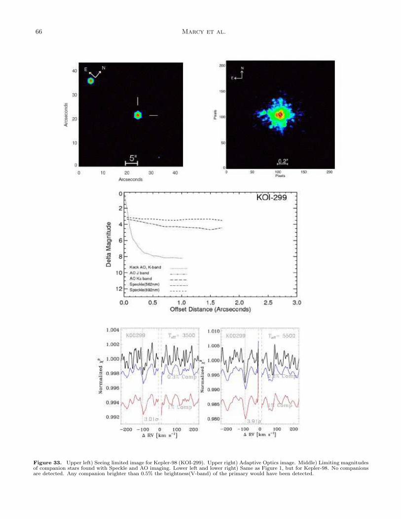
66 Marcy et al.

Figure 33. Upper left) Seeing limited image for Kepler-98 (KOI-299). Upper right) Adaptive Optics image. Middle) Limiting magnitudesof companion stars found with Speckle and AO imaging. Lower left and lower right) Same as Figure 1, but for Kepler-98. No companionsare detected. Any companion brighter than 0.5% the brightness(V-band) of the primary would have been detected.

Kepler Planet Masses 67

Figure 34. Top) RV versus time for Kepler-98 (KOI-299). Middle) Phase folded radial velocities for each planet. Bottom) Phase foldedKepler photometry for the transiting planet. The blue points represent binned RVs near quadrature, same as Figure 2. Kepler-98b: Rp =1.99± 0.22 R⊕, Mp = 3.55± 1.6 M⊕.

68 Marcy et al.

Figure 35. Upper left) Seeing limited image for Kepler-99 (KOI-305). Upper right) Adaptive Optics image. Middle) Limiting magnitudesof companion stars found with Speckle and AO imaging. Lower left and lower right) Same as Figure 1, but for Kepler-99. No companionsare detected. Any companion brighter than 0.5% the brightness(V-band) of the primary would have been detected.

Kepler Planet Masses 69

Figure 36. Top) RV versus time for Kepler-99 (KOI-305). Middle) Phase folded radial velocities for each planet. Bottom) Phase foldedKepler photometry for the planet. The blue points represent binned RVs near quadrature, same as Figure 2. Kepler-99b: Rp = 1.48±0.08R⊕, Mp = 6.15± 1.3 M⊕.

70 Marcy et al.

Figure 37. Upper left) Seeing limited image for Kepler-406 (KOI-321). Upper right) Adaptive Optics image. Middle) Limiting magnitudesof companion stars found with Speckle and AO imaging. Lower left and lower right) Same as Figure 1, but for Kepler-406. No companionsare detected. Any companion brighter than 0.5% the brightness(V-band) of the primary would have been detected.

Kepler Planet Masses 71

Figure 38. Top) RV versus time for Kepler-406 (KOI-321). Lower left) Phase folded Kepler photometry for each planet. Lower Right)Phase folded radial velocities for each planet. The blue points represent binned RVs near quadrature, same as Figure 2. Kepler-406b: Rp= 1.43± 0.03 R⊕, Mp = 6.35± 1.4 M⊕. Kepler-406c: Rp = 0.85± 0.03 R⊕, Mp = 2.71± 1.8 M⊕.

72 Marcy et al.

Kepler Planet Masses 73

Figure 39. Upper left) Seeing limited image for Kepler-407 (KOI-1442). Upper right) Adaptive Optics image from Keck NIRC2. Middle)Limiting magnitudes of companion stars from Speckle and AO imaging. Lower left and lower right) Same as Figure 1, but for Kepler-407.No secondary lines from a companion are detected . Any companion brighter than 0.5% the brightness(V-band) of the primary would havebeen detected.

74 Marcy et al.

Figure 40. Top) RV versus time for Kepler-407 (KOI-1442). Lower left) Phase folded Kepler photometry for the transiting planet.Lower Right) Phase folded radial velocities for each planet. The blue points represent binned RVs near quadrature, same as Figure 2.Kepler-407b: Rp = 1.07±0.02 R⊕, Mp = 0.06±1.2 M⊕. Kepler-407c: Rp = NA, Mp = 4000±2000M⊕ , period = 3000±500d. Kepler-407could be a planet, brown dwarf, or a star, depending on the inclination of the orbit.

Kepler Planet Masses 75

Figure 41. Upper left) Seeing limited image for KOI-1612. Upper right) Adaptive Optics image. Middle) Limiting magnitudes ofcompanion stars found with Speckle and AO imaging. Lower left and lower right) Same as Figure 1, but for KOI-1612. No companions aredetected. Any companion brighter than 0.5% the brightness(V-band) of the primary would have been detected.

76 Marcy et al.

Figure 42. Top) RV versus time for KOI-1612. Middle) Phase folded radial velocities for each planet. Bottom) Phase folded Keplerphotometry for the planet. The blue points represent binned RVs near quadrature, same as Figure 2. KOI-1612.01: Rp = 0.82± 0.03 R⊕,Mp = 0.48± 3.2 M⊕.

Kepler Planet Masses 77

Figure 43. Upper left) Seeing limited image for Kepler-409b (KOI-1925). Upper right) Adaptive Optics image. Middle) Limitingmagnitudes of companion stars found with Speckle and AO imaging. Lower left and lower right) Same as Figure 1, but for Kepler-409. Nocompanions are detected. Any companion brighter than 0.5% the brightness(V-band) of the primary would have been detected.

78 Marcy et al.

Figure 44. Top) RV versus time for Kepler-409 (KOI-1925). Middle) Phase folded radial velocities for each planet. Bottom) Phasefolded Kepler photometry for each planet. The blue points represent binned RVs near quadrature, same as Figure 2. Kepler-409b: Rp =1.19± 0.03 R⊕, Mp = 2.69± 6.2 M⊕.

Kepler Planet Masses 79

Figure 45. Histogram of the radii of the 42 transiting planetsstudied here, most of which are smaller than 3 R⊕, with 6 greaterthan 3 R⊕. The radii were determined from full models of thetransit light curves, and stellar radii coming from analysis of highresolution spectra and, for 11 cases, asteroseismological analysis.

Figure 46. Histogram of the masses of the 42 transiting planetsstudied here. The mass determinations stem from the multiple RVmeasurements of the host star and the constrained orbital periodand measured time of transit from the Kepler photometry. Circu-lar orbits were assumed in all cases. Mass determinations representthe peak of the posterior mass distribution from the MCMC anal-ysis of the RVs. For four planets, fluctuations (errors) in the RVshappen to yield a peak in the posterior mass distribution that re-sides at a negative mass (K is negative, given the frozen orbitalphase). While unphysical, the negative masses offer an unbiasedstatistical balance against the fluctuations that yield overly posi-tive masses. The masses span a range up to 25 M⊕. See Fig 49 forthe well determined planet masses.

Figure 47. Histogram of the densities of the 42 transiting planetsstudied here. Four values of density are negative, due to negativemasses (See Fig. 46), three being offscale. The physical planet den-sities span a range from below unity to 15 g cm−3. As each densityis the mode of a broad posterior distribution, caution should beexercised in interpreting the histogram. See Figure 51 for the well-measured density measurements.

Figure 48. Planet mass vs radius for the 16 transiting planetsstudied here having a mass measured at the 2σ confidence levelor better. Planet mass increases systematically with increasing ra-dius. The weighted, linear fit to the planet masses and radii is,M = 3.28R + 0.79 (with M and R in Earth units), for planetradii in the range 1–5.5 R⊕. The monotonic relationship is consis-tent with a predominantly rocky composition for planets smallerthan ∼ 2 R⊕, and an increasing contribution of low density ma-terial (probably H, He, or light molecules) for larger planets. Thepresent data do not warrant more than a linear relationship, butsee Weiss & Marcy (2013) and Rogers et al. (2013).

80 Marcy et al.

Figure 49. Planet mass vs radius for both the 16 transiting plan-ets having a 2σ mass measurement, along with 14 upper limits tothe masses of the remaining planets. The best-fit linear relationbetween planet mass and radius is, M = 3.28R + 0.79 (with Mand R in Earth units), for planet radii in the range 1–5.5 R⊕. Theupper limits are consistent with the linear trend in M vs R foundfrom the 16 detections and their scatter. These upper limits areconsistent with mass increasing systematically with radius, as inFig. 48 Some planets appear to have masses below the linear fit atthe 2-σ level, indicating that some of them contain more volatilematerial than average for their radius, i.e. diversity of compositionfor a given radius. See Weiss & Marcy (2013) and Rogers et al.(2013) for further statistical treatment. The 12 planets with anuncertainty in density greater than 6.5 g cm−3were excluded fromthis plot.

Figure 50. Planet mass vs radius for 30 transiting planets mea-sured here. The plotted masses represent the peak of the posteriordistribution of the planet masses. Most peaks reside at positivemasses, but RV fluctuations occassionaly yield a peak at negativemasses, clearly representing non-detections. We retain the nega-tive masses to avoid Lutz-Kelker-type bias toward positive masses.The best-fit linear relation is M = 4.24R−2.29 (in Earth units) forplanet radii in the range 1–5.5 R⊕, including negative masses in thefit. Of the 42 transiting planets studied here, we excluded from thisplot the 12 transiting planets having a density uncertainty greaterthan 6.5 g cm−3(but included all mass measurements, even if lessthan a 2-sigma detection).

Figure 51. Planet density vs radius for all 30 transiting plan-ets having an uncertainty in density less than 6.5 g cm−3. Planetdensity declines systematically with increasing planet radius in thedomain of 1.0–5.5 R⊕. Increasing planet radius apparently is asso-ciated with increasing amounts of low density material, presumablyH, He, and light molecules. For an analysis of density vs radiusfor all known planets, see Weiss & Marcy (2013) and Rogers et al.2014 (in prep).

Figure 52. Planet density vs planet mass for the 30 transitingplanets measured here. Planet density appears to increase from 1to ∼6 M⊕, and then decline from ∼6–25 R⊕, with large scatter indensity. This behavior is consistent with planets of 0–6 M⊕ havinga mostly rocky interior experiencing increased gravitational com-pression (or greater iron/nickel content). The decline in density forplanet masses, M > 6 M⊕ indicates increasing amounts of low den-sity material, presumably H, He, and light molecules, with increas-ing planet mass. The scatter in planet density, at a given planetmass, indicates a diversity of chemical composition at a given mass,with different admixtures of iron, rock, and light elements.

Kepler Planet Masses 81

Figure 53. Planet radius vs orbital period for 30 well-measuredtransiting planets. Planet radii are not strongly correlated withorbital period in the present sample.

Figure 54. Planet density vs orbital period for 30 well-measuredtransiting planets. Planet density is not strongly correlated withorbital period. There is no convincing evidence that the density,and hence planet composition, is a strong function of orbital dis-tance, out to periods of 45 days. But mass detection biases mayaffect this interpretation.

Figure 55. Histogram of impact parameters, b, for all 42 tran-siting planets studied here. The impact parameter is derived froma self-consistent transiting-planet model fit to the photometry andRVs, with constraints on the stellar radius from spectroscopy andasteroseismology. The roughly uniform distribution of impact pa-rameters, from 0 to 1, is consistent with the geometrical expecta-tion of a random distribution of orbital tilt angles relative to ourline of sight, leading to a uniform distribution of impact parame-ters, b.

82

Marcyetal.

Table 1Stellar Parameters

Kepler # KOI KIC RA Dec Teff Stellar [Fe/H] M∗ R∗ V sin i Kepler Age Sourcea

(K) log g (M⊙ ) (R⊙ ) (km s−1 ) Magn. (Gyr) MCMC+

Kepler-100 41 6521045 19:25:32.6 41:59:24 5825 ± 75 4.125± 0.03 +0.02± 0.10 1.08± 0.06 1.49± 0.04 3.7 11.20 6.46 ASKepler-93 69 3544595 19:25:40.3 38:40:20 5669 ± 75 4.468± 0.03 −0.18± 0.10 0.91± 0.06 0.92± 0.02 0.5 9.93 5.05 ASKepler-102 82 10187017 18:45:55.8 47:12:28 4903 ± 74 4.607± 0.03 +0.08± 0.07 0.80± 0.06 0.74± 0.02 0.5 11.49 1.41 SMEKepler-94 104 10318874 18:44:46.7 47:29:49 4781 ± 98 4.590± 0.04 +0.34± 0.07 0.81± 0.06 0.76± 0.03 0.5 12.90 1.41 SMEKepler-103 108 4914423 19:15:56.2 40:03:52 5845 ± 88 4.162± 0.04 +0.07± 0.11 1.09± 0.07 1.44± 0.04 2.5 12.29 5.70 ASKepler-106 116 8395660 20:03:27.3 44:20:15 5858 ± 114 4.407± 0.14 −0.12± 0.11 1.00± 0.06 1.04± 0.17 0.3 12.88 4.83 SMEKepler-95 122 8349582 18:57:55.7 44:23:52 5699 ± 74 4.171± 0.04 +0.30± 0.10 1.08± 0.08 1.41± 0.04 0.7 12.35 5.63 ASKepler-109 123 5094751 19:21:34.2 40:17:05 5952 ± 75 4.211± 0.04 −0.08± 0.10 1.04± 0.06 1.32± 0.04 1.0 12.36 5.73 ASKepler-48 148 5735762 19:56:33.4 40:56:56 5194 ± 73 4.487± 0.05 +0.17± 0.07 0.88± 0.06 0.89± 0.05 0.5 13.04 3.14 SMEKepler-113 153 12252424 19:11:59.4 50:56:39 4725 ± 74 4.636± 0.03 +0.05± 0.07 0.75± 0.06 0.69± 0.02 0.4 13.46 6.89 SMEKepler-25 244 4349452 19:06:33.2 39:29:16 6270 ± 79 4.278± 0.03 −0.04± 0.10 1.19± 0.06 1.31± 0.02 9.5 10.73 11.00 ASKepler-37 245 8478994 18:56:14.2 44:31:05 5417 ± 75 4.567± 0.05 −0.32± 0.07 0.80± 0.07 0.77± 0.03 0.5 9.70 5.66 ASKepler-68 246 11295426 19:24:07.7 49:02:24 5793 ± 74 4.282± 0.02 +0.12± 0.07 1.08± 0.05 1.24± 0.02 0.5 10.00 6.30 ASKepler-96 261 5383248 19:48:16.7 40:31:30 5690 ± 73 4.421± 0.08 +0.04± 0.07 1.00± 0.06 1.02± 0.09 0.5 10.30 2.34 SMEKepler-131 283 5695396 19:14:07.4 40:56:32 5685 ± 74 4.417± 0.08 +0.12± 0.07 1.02± 0.06 1.03± 0.10 0.4 11.52 3.66 SMEKepler-97 292 11075737 19:09:18.3 48:40:24 5779 ± 74 4.430± 0.08 −0.20± 0.07 0.94± 0.06 0.98± 0.09 0.5 12.87 8.42 SMEKepler-98 299 2692377 19:02:38.8 37:57:52 5539 ± 73 4.341± 0.10 +0.18± 0.07 0.99± 0.06 1.11± 0.12 0.5 12.90 2.79 SMEKepler-99 305 6063220 19:49:24.9 41:18:00 4782 ± 129 4.605± 0.05 +0.18± 0.07 0.79± 0.06 0.73± 0.04 0.5 12.97 1.47 SMEKepler-406 321 8753657 19:27:23.5 44:58:05 5538 ± 75 4.409± 0.02 +0.18± 0.07 1.07± 0.06 1.07± 0.02 0.4 12.52 5.84 ASKepler-407 1442 11600889 19:04:08.7 49:36:52 5476 ± 75 4.426± 0.06 +0.33± 0.07 1.00± 0.06 1.01± 0.07 2.0 12.52 7.47 SME· · · 1612 10963065 18:59:08.6 48:25:23 6104 ± 74 4.294± 0.03 −0.20± 0.10 1.08± 0.07 1.23± 0.03 3.1 8.77 6.68 ASKepler-409 1925 9955598 19:34:43.0 46:51:09 5460 ± 75 4.499± 0.03 +0.08± 0.10 0.92± 0.06 0.89± 0.02 2.0 9.44 6.80 AS

Kepler Planet Masses 83

a “AS”: Asteroseismology provided the input stellarvalues of Teffand log g to the MCMC analysis of theplanet-transit model that further constrained stellar pa-rameters. LTE spectrum synthesis, SME, yielded initialmeasurements of Teff , log g, and metallicity, used as in-put values and priors for the asteroseismology analysis.“SME”: the SME code performed LTE spectrum anal-ysis to yield Teff , log g, and metalicity, used as inputto the MCMC analysis of the planet transit model. It-eration with Yonsei-Yale stellar models constrained allstellar values.

84

Marcyetal.

Table 2Planet Properties and Orbital Parameters

Kepler # KOI Perioda Radiusb Mass(peak)c Massd Planet Densitye Kf Stellar density Impact RP/R∗ Midtransit E Reduced Chi2

(days) (R⊕ ) (M⊕ ) 95%(M⊕ ) (g cm−3) (m s−1 ) (g cm−3) Param. (b) (BJD-2454900)

Kepler-100c 41.01 12.8159 2.20± 0.05 0.85± 4.0 7.05 0.35± 1.65 0.18± 0.8 0.44± 0.01 0.05 ± 0.04 0.013550 55.94713 1.185Kepler-100b 41.02 6.88705 1.32± 0.04 7.34± 3.2 10.0 14.25± 6.33 1.90± 0.8 0.44± 0.01 0.54 ± 0.02 0.008094 66.17797 1.110Kepler-100d 41.03 35.3331 1.61± 0.05 −4.36± 4.1 3.0 −5.72± 6.00 −0.79± 1.0 0.44± 0.01 0.75 ± 0.01 0.009926 86.98031 1.261Kepler-93b 69.01 4.72674 1.50± 0.03 2.59± 2.0 6.1 4.17± 3.29 1.05± 0.8 1.64± 0.01 0.20 ± 0.02 0.014927 67.92580 1.017Kepler-93c 69.10g >1460 · · · >954 · · · · · · >60 · · · · · · · · · · · · · · ·

Kepler-102e 82.01 16.1457 2.22± 0.07 8.93± 2.0 11.7 4.68± 1.12 2.77± 0.6 2.76± 0.09 0.30 ± 0.03 0.027639 67.75384 1.026Kepler-102d 82.02 10.3117 1.18± 0.04 3.80± 1.8 6.6 13.27± 6.46 1.37± 0.6 2.76± 0.09 0.22 ± 0.05 0.014682 67.07920 0.950Kepler-102f 82.03 27.4536 0.88± 0.03 0.62± 3.3 5.2 4.92± 24.5 2.11± 0.8 2.76± 0.09 0.57 ± 0.03 0.010963 78.02565 1.404Kepler-102c 82.04 7.07142 0.58± 0.02 −1.58± 2.0 3.0 −44.24± 56.7 −1.00± 0.6 2.76± 0.09 0.06 ± 0.05 0.007228 72.98486 0.883Kepler-102b 82.05 5.28696 0.47± 0.02 0.41± 1.6 4.3 23.29 ± 94.93 0.19± 0.7 2.76± 0.09 0.06 ± 0.06 0.005800 68.84920 0.958Kepler-94b 104.01 2.50806 3.51± 0.15 10.84± 1.4 16.5 1.45± 0.26 6.11± 0.8 2.90± 0.23 0.85 ± 0.01 0.042380 67.99980 1.076Kepler-94c 104.10h 820.3± 3 · · · 3126 ± 200 4321 · · · 262.7± 13.9 · · · · · · · · · · · · · · ·

Kepler-103b 108.01 15.9654 3.37± 0.09 9.7± 8.6 30.0 1.38 ± 1.4 2.32± 2.1 0.52± 0.02 0.72 ± 0.01 0.021500 75.17614 0.866Kepler-103c 108.02 179.612 5.14± 0.14 36.10 ± 25.2 95 1.47 ± 1.2 3.85± 2.7 0.52± 0.02 0.44 ± 0.02 0.032766 228.32581 0.824Kepler-106c 116.01 13.5708 2.50± 0.32 10.44± 3.2 18.8 3.28± 1.56 2.71± 0.8 1.38± 0.15 0.69 ± 0.03 0.022113 69.27837 1.000Kepler-106e 116.02 43.8445 2.56± 0.33 11.17± 5.8 24.8 3.10± 2.07 1.95± 1.0 1.38± 0.15 0.28 ± 0.13 0.022676 84.93360 0.933Kepler-106b 116.03 6.16486 0.82± 0.11 0.15± 2.8 5.3 1.26± 26.26 0.05± 0.9 1.38± 0.15 0.39 ± 0.15 0.007258 68.64035 0.992Kepler-106d 116.04 23.9802 0.95± 0.13 −6.39± 7.0 8.1 −41.00± 39.75 −2.84± 0.9 1.38± 0.15 0.45 ± 0.11 0.008362 80.53263 1.051Kepler-95b 122.01 11.5231 3.42± 0.09 13.0± 2.9 16.7 1.71± 0.37 3.36± 0.6 0.54± 0.02 0.74 ± 0.01 0.022166 64.96841 0.891Kepler-109b 123.01 6.48163 2.37± 0.07 1.3± 5.4 7.3 0.3± 2.2 0.29± 1.8 0.65± 0.02 0.58 ± 0.02 0.016434 55.97755 1.000Kepler-109c 123.02 21.2227 2.52± 0.07 2.22± 7.8 21.8 0.65± 2.30 0.43± 1.5 0.65± 0.02 0.16 ± 0.08 0.017432 70.57250 0.975Kepler-48b 148.01 4.77800 1.88± 0.10 3.94± 2.1 13.0 3.23± 1.84 1.62± 0.9 1.98± 0.13 0.17 ± 0.11 0.019318 57.06113 0.933Kepler-48c 148.02 9.67395 2.71± 0.14 14.61± 2.3 22.7 4.01± 0.91 4.74± 0.7 1.98± 0.13 0.38 ± 0.05 0.027892 58.33925 0.992Kepler-48d 148.03 42.8961 2.04± 0.11 7.93± 4.6 25.0 5.08± 3.12 1.57± 0.9 1.98± 0.13 0.20 ± 0.11 0.021021 79.06554 0.976Kepler-48e 148.10 982 ± 8 · · · 657 ± 25 727 · · · 45.83 ± 0.8 · · · · · · · · · · · · · · ·

Kepler-113c 153.01i 8.92507 2.18± 0.06 −4.04± 6.4 8.7 −2.13± 3.4 −1.52± 2.4 2.71± 0.08 0.56 ± 0.02 0.029135 72.71374 0.950Kepler-113b 153.02i 4.75400 1.82± 0.05 11.7± 4.2 20. 10.73± 3.9 5.4± 1.9 2.71± 0.08 0.08 ± 0.06 0.024190 61.54630 0.950Kepler-25c 244.01 12.7204 5.20± 0.09 24.60± 5.7 32.4 0.90± 0.21 5.63± 1.3 0.75± 0.01 0.88 ± 0.00 0.036409 111.52730 1.127Kepler-25b 244.02 6.2385 2.71± 0.05 9.6± 4.2 16.0 2.50± 1.10 2.80± 1.2 0.75± 0.01 0.54 ± 0.01 0.018950 104.70541 1.051Kepler-25d 244.10h 123 ± 2 · · · 89.90 ± 13.7 101 · · · 9.67± 1.5 · · · · · · · · · · · · · · ·

Kepler-37d 245.01 39.7922 1.94± 0.06 1.87± 9.08 12.2 1.30± 3.67 0.40± 1.2 2.46± 0.04 0.53 ± 0.01 0.023068 108.24950 1.160Kepler-37c 245.02 21.3020 0.75± 0.03 3.35± 4.0 12.0 44.33 ± 53.60 0.92± 1.1 2.46± 0.04 0.43 ± 0.02 0.008909 124.83685 1.227Kepler-37b 245.03 13.3675 0.32± 0.02 2.78± 3.7 10.0 548.8 ± 700.0 0.95± 1.1 2.46± 0.04 0.48 ± 0.13 0.003828 117.04171 0.950Kepler-68b 246.01 5.39875 2.33± 0.02 5.97± 1.7 9.3 2.60± 0.74 2.07± 0.59 0.79± 0.01 0.48 ± 0.01 0.017383 106.85783 1.076Kepler-68c 246.02 9.60504 1.00± 0.02 2.18± 3.5 7.2 10.77 ± 17.29 0.57± 0.9 0.79± 0.01 0.77 ± 0.01 0.007455 69.38025 1.084Kepler-68d 246.10h 625± 16 · · · 267 ± 16 283 · · · 19.06± 0.58 · · · · · · · · · · · · · · ·

Kepler-96b 261.01 16.2385 2.67± 0.22 8.46± 3.4 12.0 2.26± 1.11 2.10± 0.8 1.54± 0.25 0.54 ± 0.07 0.023967 104.01897 1.219Kepler-131b 283.01 16.0920 2.41± 0.20 16.13± 3.5 19.4 6.00± 1.98 3.95± 0.8 1.44± 0.21 0.79 ± 0.02 0.021263 103.59795 1.051Kepler-131c 283.02 25.5169 0.84± 0.07 8.25± 5.9 20.0 77.7 ± 55. 3.58± 0.9 1.44± 0.21 0.27 ± 0.16 0.007394 87.42342 0.891Kepler-97b 292.01 2.58664 1.48± 0.13 3.51± 1.9 9.1 5.44± 3.48 1.65± 0.9 1.53± 0.31 0.41 ± 0.16 0.013803 104.84121 0.950Kepler-97c 292.10g >789 · · · >344 · · · · · · >25 · · · · · · · · · · · · · · ·

Kepler-98b 299.01 1.54168 1.99± 0.22 3.55± 1.6 6.4 2.18± 1.21 1.82± 0.8 1.12± 0.34 0.56 ± 0.14 0.016377 103.54328 0.950Kepler-99b 305.01 4.60358 1.48± 0.08 6.15± 1.3 9.7 10.90± 2.82 2.91± 0.6 2.86± 0.23 0.21 ± 0.13 0.018475 104.83893 0.992Kepler-406b 321.01 2.42629 1.43± 0.03 6.35± 1.4 8.1 11.82± 2.70 2.89± 0.6 1.12± 0.02 0.10 ± 0.06 0.012285 103.45680 1.093Kepler-406c 321.02 4.62332 0.85± 0.03 2.71± 1.8 6.0 24.39 ± 16.13 1.00± 0.6 1.12± 0.02 0.36 ± 0.06 0.007261 65.37438 0.883Kepler-407b 1442.01 0.669310 1.07± 0.02 0.06± 1.2 3.2 0.29± 5.70 0.05± 0.9 1.38± 0.16 0.25 ± 0.15 0.010414 67.13162 0.958Kepler-407c 1442.10g 3000 ± 500 · · · 4000 ± 2000 8000 · · · 164 ± 20 · · · · · · · · · · · · · · ·

· · · 1612.01 2.46502 0.82± 0.03 0.48± 3.2 5.0 4.42± 29.82 0.20± 1.3 0.82± 0.01 0.92 ± 0.01 0.006136 65.67928 0.849Kepler-409b 1925.01 68.9584 1.19± 0.03 2.69± 6.2 22.0 8.88± 20.60 0.45± 1.0 1.81± 0.00 0.90 ± 0.01 0.012223 112.08151 1.059

Kepler Planet Masses 85

a Each planet’s orbital period is determined using onlythe Kepler photometry.

b Each planet’s radius is measured using the combinedRV/photometry analysis, consistent with the best valuesfound for the stellar mass and radius. Errors are domi-nated by uncertainties in the stellar radius.

c Each planet mass is calculated using the combinedRV/photometry analysis. The stellar parameters arethose found in Table 1. The peak of the posterior distri-bution for the planet mass is chosen as the best value.The peak can have either a positive or negative value.

d We choose the 95th percentile of the MCMC distri-bution as the upper limit to the mass. We choose tolist this value for all planets, but these values are moremeaningful when the mass detection is marginal or themass is poorly constrained.

e Planets with measurements of density greater than5 g cm−3are typed with bold font, including only thosewith RV mass detections at the 2σ level or better. Theseplanets likely have interior compositions that are mostlyrock and iron/nickel. We caution that planets havingmeasured densities only 2–3 σ above zero require moreRV measurements to secure their rocky nature. Twoother planets with densities between 4-5 g cm−3are alsolikely rocky, namely Kepler-102e and Kepler-48c.

f The RV amplitude listed is the peak of the posteriordistribution for the combined RV/photometry fit. Un-certainties are determining by integrating the posteriordistribution out from the peak value until 68% of thevalues in the MCMC chain are included.

gLong term variation in RVs indicates a long periodorbiting object, which may not be a planet (Marcy et al.2001).

h A floating orbital eccentricity was allowed in themodel for the outer, non-transiting planet, as indi-cated by apparent non-sinusoidal long-term variationin the RVs, for Kepler-94, Kepler-25, and Kepler-68.The best-fit eccentricities are 0.38±0.05, 0.18±0.10, and0.10±0.04, respectively. See notes in Section 7 on theindividual KOIs for more information.

i For Kepler-113, the RV residuals to the fit to thetwo transiting planets indicate the presence of a third,non-transiting planet. The highest periodogram peak isat a period, P = 1.065 d. But peaks appear at aliases,namely at 16 d, 0.984 d, and 0.515 d. We are not ableto determine which among this family of alias periods isthe real period, if any, thus we are not able to assuredlysuggest the period or existence of this prospective non-transiting planet around Kepler-113.

86 Marcy et al.

Table 3False Positive Probabilities

Kepler # KOI rExcl. [“]a Comp. sep.[“]b PEB PHEB PBGEB PBGPL Priorc

PLFPPd

Kepler-100c 41.01 4-SAT single <1e-4 <1e-4 <1e-4 <1e-4 0.56 <1e-4Kepler-100b 41.02 4-SAT single <1e-4 <1e-4 <1e-4 <1e-4 0.25 <1e-4Kepler-100d 41.03 4-SAT single <1e-4 <1e-4 <1e-4 <1e-4 0.37 <1e-4Kepler-93b 69.01 4-SAT single <1e-4 <1e-4 <1e-4 <1e-4 0.33 <1e-4Kepler-102e 82.01 4-SAT single <1e-4 <1e-4 <1e-4 <1e-4 0.56 <1e-4Kepler-102d 82.02 4-SAT single <1e-4 <1e-4 <1e-4 <1e-4 0.18 <1e-4Kepler-102f 82.03 4-SAT single <1e-4 <1e-4 <1e-4 <1e-4 0.07 <1e-4Kepler-102c 82.04 4-SAT single <1e-4 <1e-4 2.5e-4 0.89e-4 0.01 3.4e-4Kepler-102b 82.05 4-SAT single <1e-4 <1e-4 7.6e-4 0.2e-4 0.00 7.8e-4Kepler-94b 104.01 0.035 single <1e-4 <1e-4 <1e-4 <1e-4 0.34 <1e-4Kepler-103b 108.01 0.009 2.44,4.87 <1e-4 <1e-4 <1e-4 <1e-4 0.37 <1e-4Kepler-103c 108.02 0.04 2.44,4.87 <1e-4 1e-4 <1e-4 <1e-4 0.13 1e-4Kepler-106c 116.01 0.23 single <1e-4 <1e-4 <1e-4 <1e-4 0.55 <1e-4Kepler-106e 116.02 0.49 single <1e-4 <1e-4 <1e-4 <1e-4 0.53 <1e-4Kepler-106b 116.03 0.83 single <1e-4 <1e-4 <1e-4 <1e-4 0.05 <1e-4Kepler-106d 116.04 2.1 single <1e-4 <1e-4 0.2e-4 1.4e-4 0.09 1.7e-4Kepler-95b 122.01 0.12 4.1 <1e-4 <1e-4 <1e-4 <1e-4 0.37 <1e-4Kepler-109b 123.01 0.11 2.03,5.3 <1e-4 <1e-4 <1e-4 <1e-4 0.56 <1e-4Kepler-109c 123.02 0.09 2.03,5.3 <1e-4 <1e-4 <1e-4 <1e-4 0.55 <1e-4Kepler-48b 148.01 0.16 2.44e <1e-4 <1e-4 <1e-4 <1e-4 0.54 <1e-4Kepler-48c 148.02 0.26 2.44e <1e-4 <1e-4 <1e-4 <1e-4 0.45 <1e-4Kepler-48d 148.03 0.28 2.44e <1e-4 <1e-4 <1e-4 <1e-4 0.56 <1e-4Kepler-113c 153.01 0.14 5.14 <1e-4 <1e-4 <1e-4 <1e-4 0.56 <1e-4Kepler-113d 153.02 0.09 5.14 <1e-4 <1e-4 <1e-4 <1e-4 0.47 <1e-4Kepler-25c 244.01 4-SAT single <1e-4 <1e-4 <1e-4 <1e-4 0.12 <1e-4Kepler-25b 244.02 4-SAT single <1e-4 <1e-4 <1e-4 <1e-4 0.51 <1e-4Kepler-37d 245.01 4-SAT single <1e-4 <1e-4 <1e-4 <1e-4 0.50 <1e-4Kepler-37c 245.02 4-SAT single <1e-4 <1e-4 <1e-4 <1e-4 0.04 <1e-4Kepler-37b 245.03 4-SAT single <1e-4 <1e-4 0.001 <1e-4 0.01 4e-4g

Kepler-68b 246.01 4-SAT single <1e-4 <1e-4 <1e-4 <1e-4 0.55 <1e-4Kepler-68c 246.02 4-SAT single <1e-4 <1e-4 6.2e-4 <1e-4 0.15 6.3e-4Kepler-96b 261.01 4-SAT 5.4 <1e-4 <1e-4 <1e-4 <1e-4 0.53 <1e-4Kepler-131b 283.01 4-SAT 6 <1e-4 <1e-4 <1e-4 <1e-4 0.55 <1e-4Kepler-131c 283.02 4-SAT 6 <1e-4 <1e-4 9.8e-04 <1e-4 0.06 9.8e-4Kepler-97b 292.01 0.20 0.38f <1e-4 <1e-4 <1e-4 <1e-4 0.31 <1e-4Kepler-98b 299.01 0.15 single <1e-4 <1e-4 <1e-4 <1e-4 0.52 <1e-4Kepler-99b 305.01 0.18 single <1e-4 <1e-4 <1e-4 <1e-4 0.31 <1e-4Kepler-406b 321.01 0.24 single <1e-4 <1e-4 <1e-4 <1e-4 0.30 <1e-4Kepler-406c 321.02 0.20 single <1e-4 <1e-4 <1e-4 <1e-4 0.06 <1e-4Kepler-407b 1442.01 0.33 2.1 <1e-4 <1e-4 <1e-4 <1e-4 0.14 <1e-4· · · 1612.01 4-SAT single <1e-4 <1e-4 2.1e-2 1.9e-4 0.05 0.021Kepler-409b 1925.01 4-SAT single <1e-4 <1e-4 3.2e-4 <1e-4 0.18 3.2e-4

Kepler Planet Masses 87

a The exclusion radius is the maximum angular dis-tance to any neighboring star that might cause the pe-riodic dimming. It is computed from the upper limitto the displacement of the photo-center during times of“transit.” This upper limit yields a maximum angulardistance to any star that could cause the apparent tran-sit. Stars farther away can’t be responsible. The note4-SAT denotes saturated images from Kepler , limitingastrometric accuracy to 4′′ (one pixel).

b Detected companions within 6′′ of the target star,found by AO or speckle observations. Keck adaptive op-tics imaging was performed on all 22 KOIs, giving thehighest resolution (0.′′050) and best contrast detectabil-ity (8 mag at K ′ bandpass, i.e., 2.2 µ). “Single” denotesno such companions. Otherwise we list the angular sep-aration in arcsec, (see Sec 7). The detection thresholdsfrom Keck Adaptive Optics and from all AO and speckleobservations for each KOI are described in 7, and plottedin Figures 1 - 44.

c The planet prior represents the probability for a starto host a planet of that approximate size (between 2/3and 4/3 the candidate’s radius), used in the FPP cal-culation. This number is based on an approximate oc-currence rate estimate using the Kepler candidates, cor-rected for transit probability, but not for individual de-tectability. For cases in which this planet prior is verysmall (e.g., for Kepler-102c and Kepler-102b), there arevery few detected candidates in this radius range, andthe true planet prior should be higher.

d The False-Positive Probability for the Planet: Thesum of the probabilities of all false-positive scenarios di-vided by the sum of probabilities of all scenarios includ-ing that the planet is real.

e For Kepler-48, there are four neighboring stars withseparations and delta magnitudes (J-band): (2.′′44,4.9),(4.′′32,3.3), (4.′′39,7.3), (5.′′89,7.0) (Adams et al. 2012).

f Kepler-97: The neighbor (0.′′36) is farther than theastrometric maximum radius (0.′′2). Thus, the planetprobably doesn’t orbit neighbor.

g Careful false positive analysis by Barclay et al.(2013) shows FPP = 0.0004.

88 Marcy et al.

Table 4Radial Velocities for KOI-41, Kepler-100

Radial Velocity Uncertainty log R′HK

BJD – 2450000 (m s−1) (m s−1)

4989.010954 -4.46 3.73 -5.0285042.015300 -11.82 3.81 -5.0345042.022823 -9.46 3.86 -5.0285042.030068 -6.02 3.77 -5.0415042.842452 -3.45 3.63 -5.0415042.849778 8.90 3.75 -5.0145044.044453 5.07 3.73 -5.0345044.051871 3.30 3.77 -5.0145044.059302 0.62 3.73 -5.0285048.909978 -7.17 3.93 -5.0145073.846868 -1.39 3.70 -5.0415074.844066 0.39 3.59 -5.0345075.868856 3.61 3.67 -5.0285076.756808 6.56 3.65 -5.0215077.894672 -9.78 3.64 -5.0485078.934772 -3.54 3.71 -5.0145079.962974 -0.23 3.71 -5.0415081.002505 -3.08 3.55 -4.9535082.982668 2.99 3.77 -5.0415312.060754 -1.25 2.78 -5.0415400.916085 2.42 2.62 -5.1095760.064528 -1.11 2.51 -5.0415760.958645 3.39 2.56 -5.0415761.876117 5.12 2.48 -5.0485762.912248 6.33 2.42 -5.0415763.870182 5.01 2.45 -5.0345791.871645 -1.99 2.47 -5.0485793.996566 -2.77 2.55 -5.0705795.012741 -12.15 3.13 -5.0855796.793068 1.87 2.42 -5.0215797.853511 5.06 2.41 -5.0415798.773192 1.43 2.37 -5.0485807.741761 2.21 2.55 -5.0705808.840217 -5.33 2.61 -5.0285809.749926 2.75 2.45 -5.0485810.749216 4.68 2.42 -5.0415811.865319 6.67 2.40 -5.0415814.757203 2.23 2.47 -5.0486109.979987 4.30 2.46 -5.0556110.856162 0.99 2.59 -5.0556111.867315 0.32 2.56 -5.0556112.888295 4.29 2.49 -5.0556113.851194 1.74 2.65 -5.1176114.900100 3.51 2.56 -5.0346115.897107 7.42 2.53 -5.0486173.889875 -1.85 2.47 -5.0556177.929359 -7.30 3.07 -5.0486178.805849 1.60 2.44 -5.0486209.725678 -0.93 2.55 -5.063

Table 5Radial Velocities for KOI-69, Kepler-93

Radial Velocity Uncertainty log R′HK

BJD – 2450000 (m s−1) (m s−1)

5044.067242 -12.90 2.73 -4.9835045.039518 -19.29 2.85 -4.9725074.010142 -11.01 2.44 -4.9725075.008297 -13.22 2.45 -4.9835075.985757 -11.06 2.43 -4.9725077.017498 -14.77 2.48 -4.9945078.016299 -16.70 2.47 -4.9725078.943562 -14.89 2.44 -4.9725079.935707 -13.23 2.39 -4.9725080.753597 -7.78 2.38 -4.9725080.792010 -9.66 2.44 -4.9665081.769317 -8.65 2.59 -4.9665081.776018 -10.64 2.71 -4.9775082.741078 -6.95 2.47 -4.966

Table 5 — Continued

Radial Velocity Uncertainty log R′HK

BJD – 2450000 (m s−1) (m s−1)

5083.753822 -6.48 2.43 -4.9665084.751762 -5.96 2.39 -4.9615373.033115 -2.16 2.41 -4.9775377.938646 -2.78 2.38 -4.9665696.963643 12.83 2.57 -4.9775697.938827 9.94 2.42 -4.9775698.937161 7.95 2.45 -4.9725700.017234 14.34 2.39 -4.9725723.039490 7.80 2.47 -4.9775759.820878 6.04 2.51 -4.9835760.863548 12.19 2.43 -4.9725762.926837 6.74 2.40 -4.9835768.842459 11.17 2.44 -4.9835807.767167 16.08 2.47 -5.0056110.033656 19.10 2.50 -4.9726115.033413 22.14 2.45 -4.9776148.820507 28.18 2.56 -4.9726174.837273 22.79 2.36 -4.972

Table 6Radial Velocities for KOI-82, Kepler-102

Radial Velocity Uncertainty log R′HK

BJD – 2450000 (m s−1) (m s−1)

5312.078536 -5.59 2.39 -4.5865373.830100 -0.92 2.40 -4.6185402.922434 -4.08 2.31 -4.6585414.824561 2.83 2.30 -4.6255428.776770 -0.60 2.33 -4.6445431.766490 -4.13 2.30 -4.6445439.774551 0.28 2.27 -4.4845440.884419 3.01 2.31 -4.6675752.082671 -1.28 2.41 -4.5735752.923634 -0.57 2.54 -4.5945752.940613 -0.33 2.60 -4.5875759.888028 1.25 2.33 -4.5865760.825411 -2.10 2.32 -4.6015787.782634 7.80 2.32 -4.5985788.796321 8.08 2.32 -4.6045794.989286 -5.42 2.47 -4.5615795.870970 -1.38 2.32 -4.5635809.768343 -1.66 2.31 -4.6335810.766141 -0.21 2.29 -4.6365811.846830 0.54 2.28 -4.6175814.775163 2.23 2.31 -4.5946110.049088 2.21 2.41 -4.6266110.877659 1.30 2.33 -4.6046111.885201 -1.67 2.32 -4.6036112.910601 4.16 2.36 -4.5816113.892412 4.91 2.38 -4.6106115.097881 3.01 2.60 -4.6246133.877339 -3.08 2.34 -4.6206134.913293 -9.37 2.37 -4.6246141.045454 1.27 2.40 -4.6306144.835181 0.78 2.37 -4.6366145.835817 3.49 2.27 -4.6306166.822306 -10.67 2.46 -4.6716172.780889 -1.06 2.42 -4.6416208.797480 9.06 2.41 -4.580

Table 7Radial Velocities for KOI-104, Kepler-94

Radial Velocity Uncertainty log R′HK

BJD – 2450000 (m s−1) (m s−1)

5377.841906 -65.50 2.75 -4.638

Kepler Planet Masses 89

Table 7 — Continued

Radial Velocity Uncertainty log R′HK

BJD – 2450000 (m s−1) (m s−1)

5378.934287 -54.36 2.96 -4.6165379.961656 -66.73 3.07 -4.7015433.761242 -11.72 2.60 -4.6855434.927884 -16.61 2.80 -4.6565438.852111 1.55 3.20 -4.8575438.881509 9.99 2.98 -4.7565465.829854 28.56 3.26 -4.4245521.729851 56.90 3.14 -4.9665697.049110 99.24 2.93 -4.6015698.037021 80.44 2.80 -4.6865699.034699 97.68 3.26 -4.6715699.997226 93.70 2.79 -4.5605723.980007 85.68 2.97 -4.5775733.960824 77.25 2.90 -4.5675734.920790 82.12 2.76 -4.5915738.849308 77.70 2.87 -4.4715759.912267 66.97 3.05 -4.8735760.882081 58.78 2.79 -4.6545789.922472 43.45 2.89 -4.9465790.939908 28.25 2.81 -4.6355798.969403 26.80 2.79 -4.6005809.956676 33.38 2.82 -4.7305810.845889 26.81 2.67 -4.5866077.025088 -285.15 2.79 -4.5766115.875911 -184.39 2.73 -4.5476135.066858 -166.59 3.17 -4.5816147.946195 -136.85 3.03 -4.5856176.762087 -90.03 2.85 -4.573

Table 8Radial Velocities for KOI-108, Kepler-103

Radial Velocity Uncertainty log R′HK

BJD – 2450000 (m s−1) (m s−1)

5073.968560 -4.76 6.71 -4.9995074.938879 -12.07 6.64 -4.9995077.005648 -7.20 7.06 -5.0545079.991586 -2.46 6.66 -5.0545080.982908 -3.87 6.66 -4.8365082.902081 5.64 6.67 -4.9995084.913610 5.06 6.63 -4.9865134.787135 -6.19 3.33 -5.0125313.104615 -2.59 2.84 -5.0065321.997726 7.95 2.89 -5.0065377.875117 -0.31 2.90 -5.0065378.838317 -0.52 3.00 -5.0265402.987989 4.71 2.91 -5.0265411.034645 0.12 2.90 -5.0065425.916614 -3.17 2.93 -5.0125433.844314 4.34 2.78 -4.9865440.822218 -2.76 2.70 -5.0065794.030378 3.36 3.14 -5.0465809.900772 -4.82 2.70 -4.999

Table 9Radial Velocities for KOI-116, Kepler-106

Radial Velocity Uncertainty log R′HK

BJD – 2450000 (m s−1) (m s−1)

5133.897351 9.29 4.06 -4.7835373.958416 6.52 3.03 -4.9485379.001449 1.61 3.29 -4.9665380.025601 -7.92 2.98 -4.9605433.918565 -3.61 3.02 -4.9205439.876430 -2.17 3.07 -4.960

Table 9 — Continued

Radial Velocity Uncertainty log R′HK

BJD – 2450000 (m s−1) (m s−1)

5441.023521 -4.05 3.23 -4.9785734.085379 0.06 3.14 -4.9605752.894726 6.75 3.20 -4.9605759.992485 -0.07 3.27 -4.9786111.910098 2.89 3.16 -4.9486113.987149 1.15 3.32 -4.9906115.949113 4.10 3.11 -4.9606133.944504 5.29 3.24 -4.9666138.981896 -5.09 3.04 -4.9606144.975318 4.26 3.35 -4.9546145.858923 4.94 3.06 -4.9546147.834465 -0.29 3.30 -4.9606151.043480 -4.99 3.19 -4.9486152.041410 -14.82 3.46 -5.0036153.049571 -3.34 3.56 -5.0746166.790534 -4.91 3.15 -4.9486173.825374 0.14 3.12 -4.9666178.784524 -8.28 3.07 -4.9666207.805559 8.16 3.34 -4.948

Table 10Radial Velocities for KOI-122, Kepler-95

Radial Velocity Uncertainty log R′HK

BJD – 2450000 (m s−1) (m s−1)

5073.994534 -2.19 6.81 -5.0025075.946624 3.90 6.80 -4.9915076.769704 -0.63 6.72 -4.9745079.919778 2.64 6.81 -5.0145080.930639 -8.02 6.81 -5.0145081.929904 -4.97 6.79 -4.9965082.942536 -7.91 6.78 -5.0025083.865170 -3.44 6.76 -5.0145084.842177 -3.48 6.71 -4.9685313.064246 -9.40 2.50 -4.9915318.098919 4.62 2.67 -4.9915377.020314 8.40 2.53 -4.9855400.944047 -0.41 2.80 -5.0085405.939014 3.36 2.57 -4.9965411.002552 5.55 2.49 -4.9745411.896640 11.00 2.65 -4.9795427.839158 -2.81 2.59 -5.0085428.800667 0.84 2.49 -4.9965434.798117 -2.08 2.44 -4.9965439.834670 -2.72 2.42 -5.0085486.806230 -2.87 2.86 -5.0265697.081519 4.67 2.68 -5.0395698.069331 2.09 2.60 -5.0335699.066159 -1.67 2.63 -5.0455700.096380 1.79 2.65 -5.0335738.817453 -3.66 2.67 -5.0145791.763490 4.17 2.48 -4.9635797.013255 1.95 2.77 -5.0455809.927350 -2.30 2.47 -5.0145814.898557 3.18 2.52 -5.0266152.011007 1.33 2.64 -4.985

Table 11Radial Velocities for KOI-123, Kepler-109

Radial Velocity Uncertainty log R′HK

BJD – 2450000 (m s−1) (m s−1)

5074.992468 7.66 7.12 -5.0145075.969200 6.70 7.11 -5.0075076.849395 9.48 7.05 -4.994

90 Marcy et al.

Table 11 — Continued

Radial Velocity Uncertainty log R′HK

BJD – 2450000 (m s−1) (m s−1)

5080.956368 -10.35 7.11 -5.0215082.920913 6.64 7.13 -4.9945083.964085 5.57 7.21 -5.0005084.949365 7.55 7.11 -4.9945170.755814 -7.51 3.49 -5.0005314.059619 -6.09 2.80 -5.0075321.104302 -1.74 2.85 -5.0215343.073868 -10.93 2.97 -5.0285344.098191 -6.20 3.10 -5.0285372.963165 -0.29 3.02 -5.0075378.870526 -0.34 2.97 -5.0216166.844942 -5.35 2.91 -4.994

Table 12Radial Velocities for KOI-148, Kepler-48

Radial Velocity Uncertainty log R′HK

BJD – 2450000 (m s−1) (m s−1)

5074.026507 -1.31 12.26 -4.8795075.032090 -1.48 12.21 -4.8595076.799857 -2.81 12.08 -4.8735077.955169 1.14 12.19 -4.8655077.975134 -8.53 12.17 -4.8795312.106882 38.33 3.16 -4.8735377.908091 18.04 2.79 -4.8485381.054562 31.24 2.83 -4.8765407.078286 32.63 2.97 -4.8205414.941524 18.40 2.73 -4.8135434.897144 6.44 2.55 -4.8405438.783842 24.56 2.77 -4.8105438.811770 25.55 2.92 -4.8135787.843659 -55.28 2.86 -4.8185793.775124 -59.11 2.85 -4.8335796.821157 -48.12 2.63 -4.8105797.947000 -49.70 2.66 -4.8285799.028618 -53.15 2.90 -4.8185807.829071 -49.37 2.92 -4.8355810.977776 -48.64 2.89 -4.8335811.953784 -53.35 2.60 -4.8435814.865587 -52.15 2.75 -4.8436115.912076 16.62 3.13 -4.7916141.025441 12.07 3.22 -4.8406145.890599 36.27 3.17 -4.8516164.829375 48.32 3.11 -4.8256173.848569 37.85 2.91 -4.8486208.750960 33.64 3.07 -4.810

Table 13Radial Velocities for KOI-153, Kepler-113

Radial Velocity Uncertainty log R′HK

BJD – 2450000 (m s−1) (m s−1)

5314.091538 -7.08 2.97 -5.0185373.884706 -5.21 3.08 -5.0605376.896191 -9.70 3.07 -5.1755378.901697 -4.04 3.05 -5.0285381.020292 -8.27 3.16 -5.1335428.828387 -6.66 3.00 -5.0845435.804603 10.57 3.16 -5.2575437.846080 -7.31 3.55 -4.9455437.882874 -10.84 3.39 -5.0985697.110582 20.09 3.43 -4.8155698.004879 17.39 3.05 -4.8305699.002293 4.43 3.27 -4.7315700.066664 15.06 3.20 -4.949

Table 13 — Continued

Radial Velocity Uncertainty log R′HK

BJD – 2450000 (m s−1) (m s−1)

5735.002572 -3.16 3.13 -5.0845752.830942 -4.22 3.23 -5.0135761.058504 8.01 2.99 -5.0655789.952972 -4.86 3.20 -5.0235792.017851 -0.80 2.95 -5.0525796.872421 11.64 3.06 -5.0765811.816797 7.82 3.02 -5.0796110.983363 -5.14 3.32 -5.1496112.973425 -15.97 3.34 -5.0986144.037413 -0.53 3.27 -5.1526147.014037 -4.98 3.29 -4.965

Table 14Radial Velocities for KOI-244, Kepler-25

Radial Velocity Uncertainty log R′HK

BJD – 2450000 (m s−1) (m s−1)

5367.102834 -7.68 4.28 -5.1835376.963016 3.26 3.89 -5.1955377.950450 -2.78 3.73 -5.1725433.941912 14.54 4.22 -5.2585696.949358 12.64 3.97 -5.2075697.952294 2.17 4.29 -5.2195698.948910 -4.71 3.98 -5.2195700.027670 10.59 4.03 -5.2075734.052698 -1.17 3.67 -5.1955735.986640 -13.52 3.84 -5.2075739.049628 -2.81 4.63 -5.1955751.935799 -16.11 3.97 -5.1955752.793676 -18.65 3.70 -5.1835759.966063 5.85 3.59 -5.1955760.809525 -4.73 3.78 -5.1835761.102651 -4.29 3.67 -5.1835762.100290 5.63 4.10 -5.2075762.110117 1.44 3.86 -5.2195762.118219 -13.47 5.07 -5.1615762.891494 -3.59 3.28 -5.2075763.840742 -8.05 3.75 -5.1955768.852800 -8.83 3.90 -5.2195769.943894 8.72 4.09 -6.7895782.065146 -6.14 4.58 -5.3015787.762931 -0.92 4.28 -5.2325788.938209 -5.17 3.93 -5.2195789.798064 1.01 4.21 -5.2455789.804939 3.83 4.57 -5.2455790.755601 -3.04 3.81 -5.2325791.933168 -0.39 3.94 -5.2455792.767270 3.70 3.76 -5.2455794.925518 17.95 4.26 -5.2725796.893200 16.45 3.96 -5.2455798.759251 3.79 3.96 -5.2585806.789430 14.91 3.97 -5.2725808.797455 20.19 3.80 -5.2585810.734832 7.34 4.10 -5.2585814.927264 15.10 4.13 -5.2725903.699358 10.63 4.06 -5.2586079.872621 -1.44 4.36 -5.3336080.109747 4.40 4.07 -5.2076114.852234 3.40 4.35 -5.1616134.929891 -11.23 3.95 -5.2196139.028357 -3.47 4.17 -5.2076145.944136 -0.85 4.72 -5.2076147.806840 -5.67 4.06 -5.2196148.839914 -6.37 4.43 -5.2326152.962700 16.32 4.35 -5.2456163.794337 22.99 4.15 -5.2326194.822303 6.48 4.58 -5.2585803.3364 10.11 16.00 05809.5034 25.41 19.00 05810.4814 -10.69 25.00 05811.3940 -4.09 12.00 0

Kepler Planet Masses 91

Table 14 — Continued

Radial Velocity Uncertainty log R′HK

BJD – 2450000 (m s−1) (m s−1)

5828.2935 -5.79 10.00 05855.2837 -9.89 19.00 05857.2627 -15.39 17.00 05877.6963 4.21 16.00 05878.2544 1.01 16.00 05879.2661 -14.69 16.00 05882.3022 13.81 16.00 05883.2764 20.81 15.00 0

Table 15Radial Velocities for KOI-245, Kepler-37

Radial Velocity Uncertainty log R′HK

BJD – 2450000 (m s−1) (m s−1)

5313.086400 3.47 2.46 -4.9725319.116525 1.15 2.61 -4.9805376.949842 0.14 2.45 -5.0085396.019973 2.18 2.53 -4.9905400.968136 8.98 2.39 -5.1165425.934247 1.79 2.27 -5.0235433.932956 -0.32 2.28 -5.0135723.052494 -1.50 2.46 -4.9595723.100134 -1.99 2.41 -4.9545768.862142 3.46 2.29 -5.0135769.817056 1.64 2.35 -5.0135770.858798 2.72 2.36 -4.9765782.046825 -1.33 2.38 -5.0385782.900841 -1.14 2.38 -5.0035787.754366 -4.12 2.34 -5.0135788.994542 -5.71 2.40 -5.0285789.882547 0.50 2.40 -5.0235790.747253 -4.64 2.34 -5.0235791.748658 -2.62 2.39 -5.0235792.759449 -0.45 2.34 -5.0135794.938166 -0.70 2.37 -5.0285795.758577 -2.35 2.47 -5.0435796.781113 -3.02 2.38 -5.0035797.783521 -3.02 2.32 -5.0035798.751068 -10.90 2.40 -4.9996098.081597 3.20 2.52 -4.9386115.057869 -0.46 2.46 -4.9766148.956270 2.18 2.29 -4.9596163.786571 3.90 2.38 -4.9186164.745854 5.34 2.36 -4.9076166.810249 -2.70 2.46 -4.9106168.007627 2.90 2.50 -4.9386174.952383 0.01 2.40 -4.907

Table 16Radial Velocities for KOI-246, Kepler-68

Radial Velocity Uncertainty log R′HK

BJD – 2450000 (m s−1) (m s−1)

5313.081849 -5.32 2.49 -5.1445319.109464 -9.27 2.64 -5.1905322.050550 -11.90 2.34 -5.1625372.982740 -10.49 2.32 -5.1625377.929044 -9.56 2.33 -5.1535381.000211 -17.12 2.39 -5.1625396.962763 -14.26 2.50 -5.1445412.922534 -18.20 2.33 -5.1715426.913366 -15.93 2.35 -5.1195431.784060 -10.20 2.32 -5.1445434.870088 -22.55 2.33 -5.1115434.876488 -23.68 2.33 -5.111

Table 16 — Continued

Radial Velocity Uncertainty log R′HK

BJD – 2450000 (m s−1) (m s−1)

5435.931255 -19.07 2.41 -5.1625436.968463 -14.79 2.62 -5.1905436.974551 -20.13 2.65 -5.2305437.940359 -14.42 2.42 -5.1195437.949792 -13.86 2.38 -5.1035438.991420 -15.34 2.38 -5.1535439.002623 -15.28 2.42 -5.1365439.923524 -18.65 2.34 -5.1115439.931556 -20.54 2.39 -5.1275440.971227 -17.33 2.34 -5.1195440.980301 -21.55 2.37 -5.1365455.809962 -22.09 2.36 -5.0805490.829645 -17.75 2.44 -5.0885672.026425 18.02 2.27 -5.1625672.998402 14.69 2.38 -5.1715673.995774 18.86 2.42 -5.1535696.973926 21.76 2.39 -5.1445697.964434 23.88 2.46 -5.1445698.962303 17.22 2.37 -5.1535722.994969 22.64 2.42 -5.1715724.033632 27.33 2.48 -5.1715728.900947 23.73 2.48 -5.2995734.064071 25.42 2.40 -5.1715734.951047 26.01 2.38 -5.1625735.974739 24.78 2.37 -5.1625739.034181 24.27 2.46 -5.1715751.796956 18.81 2.47 -5.1625752.104703 17.96 2.40 -5.2005752.778961 15.83 2.42 -5.1625759.975172 18.93 2.40 -5.1535761.076467 22.02 2.30 -5.1535761.841845 15.82 2.35 -5.2005763.032747 19.13 2.36 -5.2205763.851041 14.98 2.36 -5.1535782.907862 15.44 2.40 -5.1715795.024254 7.43 2.53 -5.1535814.735957 13.15 2.34 -5.0956077.045184 -15.87 2.41 -5.1816098.093799 -11.87 2.46 -5.1716098.828990 -12.59 2.44 -5.1446102.007905 -5.88 2.37 -5.1626114.871876 -15.41 2.37 -5.1536145.875413 -9.89 2.45 -5.1366148.928774 -3.85 2.33 -5.1116151.060872 -10.87 2.41 -5.1276153.983044 -9.16 2.36 -5.0956174.826576 -1.05 2.45 -5.0886345.155209 17.40 2.44 -5.1626475.843586 10.26 2.45 -5.1626498.070164 3.00 2.43 -5.1626513.044113 -2.18 2.45 -5.1626519.919555 -0.24 2.39 -5.162

Table 17Radial Velocities for KOI-261, Kepler-96

Radial Velocity Uncertainty log R′HK

BJD – 2450000 (m s−1) (m s−1)

5405.030168 2.55 2.47 -4.7555405.889943 2.32 2.34 -4.7455413.976523 0.62 2.48 -4.7395431.794557 3.78 2.30 -4.7655436.986914 5.95 2.35 -4.7935437.960924 3.00 2.26 -4.7655437.971745 7.19 2.30 -4.7625438.829298 3.66 2.31 -4.7585439.855631 -3.95 2.31 -4.7585455.819605 2.30 2.38 -4.7585486.833994 1.19 2.42 -4.7755542.714646 0.82 2.46 -4.7695544.703444 -5.41 2.55 -4.576

92 Marcy et al.

Table 17 — Continued

Radial Velocity Uncertainty log R′HK

BJD – 2450000 (m s−1) (m s−1)

5723.092577 0.86 2.58 -4.6635787.903358 -3.39 2.50 -4.7585795.035974 -4.74 2.41 -4.7555795.835975 -3.78 2.57 -4.7756099.033843 5.65 2.59 -4.7086111.925286 -12.19 2.59 -4.7426145.907599 -6.48 2.52 -4.7826148.981644 5.12 2.64 -4.7796152.067220 -1.91 2.53 -4.7976163.805762 2.65 2.43 -4.7826164.846196 2.79 2.45 -4.7866175.877276 -4.53 2.47 -4.7976176.894658 -8.24 2.49 -4.786

Table 18Radial Velocities for KOI-283, Kepler-131

Radial Velocity Uncertainty log R′HK

BJD – 2450000 (m s−1) (m s−1)

5433.868391 5.08 2.30 -4.8245434.854201 4.86 2.31 -4.8285440.950440 -2.54 2.37 -4.8605471.813137 0.10 2.56 -4.8565490.808418 -0.81 2.63 -4.8565522.775891 -6.82 2.61 -4.8645542.700150 5.54 2.67 -4.8865724.012916 1.75 2.42 -4.9285734.972723 -3.99 2.43 -4.9045736.009887 -4.90 2.46 -4.9005788.893783 7.50 2.58 -4.8605795.941507 3.92 2.39 -4.8446101.059779 1.30 2.50 -4.8956110.960155 -0.31 2.58 -4.9756115.924507 6.65 2.58 -4.8916140.911995 -3.73 2.61 -4.8956164.891469 -11.47 2.52 -4.9756166.889764 -13.88 2.53 -4.9286173.867998 10.24 2.46 -4.8566175.860356 2.27 2.55 -4.840

Table 19Radial Velocities for KOI-292, Kepler-97

Radial Velocity Uncertainty log R′HK

BJD – 2450000 (m s−1) (m s−1)

5377.974537 2.05 3.02 -5.1045405.869250 3.50 2.94 -5.1205407.043984 4.70 3.08 -5.1365410.952610 3.43 2.90 -5.1205411.803603 8.88 2.95 -5.1125412.865682 4.95 3.11 -5.1285425.822700 3.24 3.03 -5.0885426.931969 2.33 2.87 -5.0885751.875319 1.94 3.30 -5.0965782.969047 2.99 3.00 -5.1205788.957075 -8.30 3.19 -5.0965790.834867 0.86 3.14 -4.9065810.874922 8.26 3.04 -5.0966103.079865 -4.15 3.45 -5.1546112.853787 -2.20 3.28 -5.1366144.947724 5.39 3.18 -5.1456145.924744 -5.74 3.05 -5.1366151.014731 -4.42 3.03 -5.1206153.016068 -15.95 3.28 ***e21476166.911312 -7.58 3.21 -5.104

Table 20 — Continued

Radial Velocity Uncertainty log R′HK

BJD – 2450000 (m s−1) (m s−1)

Table 20Radial Velocities for KOI-299, Kepler-98

Radial Velocity Uncertainty log R′HK

BJD – 2450000 (m s−1) (m s−1)

5404.011500 9.78 2.76 -4.7885406.943814 5.91 2.90 -4.8355407.871779 -1.02 2.75 -4.7945411.927391 -1.76 2.74 -4.8465413.947119 -9.22 2.91 -4.8765414.852128 -12.73 2.66 -4.8535433.792757 -5.53 2.61 -4.8115434.771547 0.81 2.61 -4.8315437.918288 3.25 2.92 -4.8425440.852924 -6.40 2.67 -4.8495735.034887 6.12 2.81 -4.7485751.843073 5.10 2.87 -4.7975760.040755 4.36 2.69 -4.7855760.909806 0.13 2.67 -4.8015796.002983 -3.74 3.22 -4.8605797.816289 5.21 2.65 -4.8315807.988113 -3.40 3.20 -4.3205810.917683 -0.34 2.67 -4.8115811.762281 -10.68 2.68 -4.8046113.004738 8.75 2.69 -4.7826114.053151 7.21 3.26 -4.9666208.773499 -3.19 2.78 -4.814

Table 21Radial Velocities for KOI-305, Kepler-99

Radial Velocity Uncertainty log R′HK

BJD – 2450000 (m s−1) (m s−1)

5404.043451 3.25 2.69 -4.4145405.840133 3.15 2.47 -4.6105406.910870 4.38 2.58 -4.7795410.923078 -4.28 2.49 -4.6765736.069898 4.67 2.69 -4.7125751.907376 -7.05 2.59 -4.6245760.980986 3.95 2.55 -4.8425790.878287 0.93 2.57 -4.6485792.968210 1.01 2.57 -4.6635795.056867 2.20 2.90 -4.6445797.876148 -1.21 2.52 -4.6286102.027398 -7.74 2.62 -4.5906112.943513 3.17 2.97 -4.6666116.071830 -5.38 2.58 -4.5916140.890738 4.76 2.59 -4.5796145.029741 1.35 2.72 -4.5896147.892714 -7.78 2.50 -4.6316163.884725 9.32 2.70 -4.5316172.829726 -1.39 2.69 -4.5936192.868451 -10.73 2.57 -4.5736195.854351 0.27 2.51 -4.559

Table 22Radial Velocities for KOI-321, Kepler-406

Radial Velocity Uncertainty log R′HK

BJD – 2450000 (m s−1) (m s−1)

5379.033747 3.62 2.57 -4.945

Kepler Planet Masses 93

Table 22 — Continued

Radial Velocity Uncertainty log R′HK

BJD – 2450000 (m s−1) (m s−1)

5380.109093 -5.92 2.66 -4.9805403.979414 3.99 2.68 -5.0075411.834541 -6.94 2.54 -5.0295412.898763 2.87 2.63 -5.0125434.825372 -0.53 2.52 -5.0855435.909173 -1.98 2.82 -5.0855751.813315 -4.74 2.76 -5.0015752.852880 -0.94 2.96 -4.9965752.868470 0.29 2.73 -4.9755759.839971 6.17 2.66 -4.9505760.936394 -4.23 2.58 -4.9655769.859474 6.60 2.56 -5.0415788.839547 -1.72 2.59 -5.0595789.984420 1.17 2.63 -5.0665810.791430 -1.37 2.51 -5.0785811.920824 -11.11 2.59 -5.1265843.811883 -7.55 3.01 -5.1486073.925432 -1.96 3.05 -4.9606075.917333 0.60 3.09 -5.0016076.992302 3.17 2.75 -4.9606098.855454 -3.04 2.44 -4.9186099.985448 0.10 2.62 -4.9416101.029734 -1.44 2.59 -4.9506101.872764 1.69 2.61 -4.9366103.050119 4.15 2.68 -4.9416104.059437 1.79 2.72 -4.9856105.064136 10.72 2.80 -4.9806109.955028 -7.50 2.49 -4.9706111.022468 1.20 2.73 -4.9656111.941178 1.24 2.53 -4.9056115.999606 4.75 2.51 -5.0016133.832918 8.11 2.57 -5.0356134.888536 -1.09 2.63 -5.0356138.008915 0.39 2.66 -5.0356140.863836 -1.40 2.69 -5.0416163.843324 -0.84 2.72 -5.0856164.774988 4.40 2.57 -5.0856166.003960 -1.82 2.71 -5.0596171.983117 -1.63 2.94 -5.0856177.836688 -6.64 2.67 -5.0786179.763596 -2.02 2.56 -5.119

Table 23Radial Velocities for KOI-1442, Kepler-407

Radial Velocity Uncertainty log R′HK

BJD – 2450000 (m s−1) (m s−1)

5697.018217 50.75 2.93 -5.0385698.101339 53.47 2.96 -5.0495699.097179 50.07 2.95 -4.9695736.037333 42.70 3.03 -5.1085752.051431 42.24 2.82 -5.0725760.015457 35.72 2.73 -5.0845760.776641 37.46 2.79 -5.0905768.875006 34.26 2.70 -5.1415769.798374 36.20 2.80 -5.1765770.841452 37.96 2.76 -5.1285790.914061 29.22 2.85 -5.0785791.889570 33.87 2.69 -5.0905792.876920 31.36 2.74 -5.0725797.899896 20.24 2.84 -5.1026133.912806 -128.73 3.07 -5.0666172.849950 -152.83 2.97 -5.0446446.924398 -255.23 3.22 -5.044

Table 24Radial Velocities for KOI-1612

Radial Velocity Uncertainty log R′HK

BJD – 2450000 (m s−1) (m s−1)

5698.087742 2.49 2.50 -4.9925699.127102 0.56 2.49 -4.9725700.112050 4.47 2.48 -5.0065700.943498 1.12 2.50 -5.0135703.924719 1.10 2.47 -5.0355704.886679 8.90 2.53 -5.0135706.894189 -3.62 2.39 -5.0285707.890606 5.94 2.47 -5.0515723.104987 -1.35 2.43 -5.0205724.114372 -5.66 2.54 -5.0285726.075420 0.17 2.36 -5.0675727.023738 -1.65 2.36 -5.0515728.890788 -1.36 2.51 -5.1785734.956730 2.31 2.45 -5.0515736.051585 -7.29 2.52 -5.0515739.066041 -3.17 2.55 -5.0435739.075902 -1.94 2.59 -5.0595751.924655 -2.95 2.50 -5.0595752.784580 -7.19 2.53 -5.0595760.075266 2.04 2.57 -5.0355761.082387 2.43 2.56 -5.0595762.898826 -0.86 2.54 -5.0755763.857299 -3.11 2.56 -5.0756000.139475 4.20 2.43 -5.0436019.033769 4.40 2.46 -5.0206020.045352 4.72 2.52 -5.0136028.005633 2.87 2.48 -4.9856073.886610 7.36 2.51 -5.0516075.968379 -4.72 2.40 -5.0756076.937976 -0.86 2.49 -5.0596098.068823 2.23 2.53 -5.0676115.023931 -5.82 2.70 -5.0756144.877583 -1.98 2.95 -5.1016145.901440 2.03 2.77 -5.0926146.966014 -1.61 2.64 -5.1016147.817037 -4.03 2.64 -5.1196148.853184 -1.97 2.55 -5.1106174.848128 -2.30 2.67 -5.138

Table 25Radial Velocities for KOI-1925, Kepler-409

Radial Velocity Uncertainty log R′HK

BJD – 2450000 (m s−1) (m s−1)

6000.146032 -2.45 2.20 -5.0616019.055308 -6.34 2.29 -5.0456020.099174 1.57 2.23 -5.0246028.041949 1.66 2.20 -5.0296073.949745 -2.48 2.23 -5.0196075.094428 -1.92 2.25 -5.0246075.977029 -1.84 2.23 -5.0246076.946404 0.74 2.27 -5.0146098.057089 -5.45 2.30 -5.0966098.838256 -0.55 2.20 -5.0616099.909720 -1.19 2.21 -5.0616100.930048 -0.06 2.16 -5.0616101.982553 0.93 2.20 -5.0566102.956964 -1.21 2.21 -5.0506103.963911 -0.88 2.22 -5.0506104.981934 2.73 2.18 -5.0616113.020955 2.76 2.21 -5.0346113.831179 1.20 2.23 -5.0456114.839891 1.39 2.24 -5.0296115.860558 6.37 2.21 -5.0456133.923304 0.39 2.31 -5.0616134.962073 -5.06 2.39 -5.0786138.035933 3.13 2.32 -5.0676148.866212 -3.70 2.30 -5.0566174.857241 5.59 2.36 -5.045

94 Marcy et al.

Table 25 — Continued

Radial Velocity Uncertainty log R′HK

BJD – 2450000 (m s−1) (m s−1)