1

Masses and compositions of three small planets orbiting the nearbyM dwarf L231-32 (TOI-270) and the M dwarf radius valley

V. Van Eylen1,2★, N. Astudillo-Defru3, X. Bonfils4, J. Livingston5, T. Hirano6,R. Luque7,8, K. W. F. Lam9, A. B. Justesen10, J. N. Winn2, D. Gandolfi11, G. Nowak7,8,E. Palle7,8, S. Albrecht10, F. Dai12, B. Campos Estrada13, J. E. Owen13, D. Foreman-Mackey14,M. Fridlund15,16, J. Korth17, S. Mathur7,8, T. Forveille4, T. Mikal-Evans18, H. L. M. Osborne1,C. S. K. Ho1, J. M. Almenara4, E. Artigau19, O. Barragán20, S. C.C. Barros21,22, F. Bouchy23,J. Cabrera24, D. A. Caldwell25, D. Charbonneau26, P. Chaturvedi27, W. D. Cochran28,S. Csizmadia24, M. Damasso29, X. Delfosse4, J. R. De Medeiros30, R. F. Díaz31, R. Doyon19,M. Esposito27, G. Fűrész32, P. Figueira33,21, I. Georgieva15, E. Goffo11, S. Grziwa18,E. Guenther27, A. P. Hatzes27, J. M. Jenkins34, P. Kabath35, E. Knudstrup10, D. W. Latham26,B. Lavie23, C. Lovis23, R.E. Mennickent36, S. E. Mullally37, F. Murgas7.8, N. Narita38,39,40,7,F. A. Pepe,23 C. M. Persson15, S. Redfield41, G. R. Ricker18, N. C. Santos21,22,S. Seager18,42,43, L. M. Serrano11, A. M. S. Smith24, A. Suárez Mascareño8, J. Subjak34,J. D. Twicken25,34, S. Udry23, R. Vanderspek42, and M. R. Zapatero Osorio44

1Mullard Space Science Laboratory, University College London, Holmbury St Mary, Dorking, Surrey RH5 6NT, UK2Department of Astrophysical Sciences, Princeton University, 4 Ivy Lane, Princeton, NJ, 08544, USA3Departamento de Matemática y Física Aplicadas, Universidad Católica de la Santísima Concepción, Alonso de Rivera 2850, Concepción, Chile4Univ. Grenoble Alpes, CNRS, IPAG, F-38000 Grenoble, France5Department of Astronomy, Graduate School of Science, The University of Tokyo, Hongo 7-3-1, Bunkyo-ku, Tokyo, 113-0033, Japan6Department of Earth and Planetary Sciences, Tokyo Institute of Technology, 2-12-1 Ookayama, Meguro-ku, Tokyo 152-8551, Japan7Departamento de Astrofísica, Universidad de La Laguna, E-38206, Tenerife, Spain8Instituto de Astrofísica de Canarias, C/ Vía Láctea s/n, E-38205, La Laguna, Tenerife, Spain9Zentrum für Astronomie und Astrophysik, Technische Universität Berlin, Hardenbergstr. 36, 10623 Berlin, Germany10Stellar Astrophysics Centre, Deparment of Physics and Astronomy, Aarhus University, Ny Munkegade 120, DK-8000 Aarhus C, Denmark11Dipartimento di Fisica, Università degli Studi di Torino, via Pietro Giuria 1, I-10125, Torino, Italy12Division of Geological and Planetary Sciences, 1200 E. California Boulevard, Pasadena, CA, 91125, USA13Astrophysics Group, Imperial College London, Blackett Laboratory, Prince Consort Road, London SW7 2AZ, UK14Center for Computational Astrophysics, Flatiron Institute, 162 Fifth Avenue, New York, NY 10010, USA15Department of Space, Earth and Environment, Chalmers University of Technology, Onsala Space Observatory, 439 92 Onsala, Sweden16Leiden Observatory, Leiden University, postbus 9513, 2300RA Leiden, The Netherlands17Rheinisches Institut für Umweltforschung, Abteilung Planetenforschung an der Universität zu Köln, Aachener Strasse 209, 50931 Köln, Germany18Department of Physics and Kavli Institute for Astrophysics and Space Research, Massachusetts Institute of Technology, Cambridge, MA 02139, USA19Institut de Recherche sur les Exoplanètes (IREx), Département de Physique, Université de Montréal, C.P. 6128, Succ. Centre-Ville, Montréal, QC, H3C 3J7, Canada20Sub-department of Astrophysics, Department of Physics, University of Oxford, Oxford, OX1 3RH, UK21Instituto de Astrofísica e Ciências do Espaço, Universidade do Porto, CAUP, Rua das Estrelas, 4150-762 Porto, Portugal22Departamento de Física e Astronomia, Faculdade de Ciências, Universidade do Porto, Rua do Campo Alegre, 4169-007 Porto, Portugal23Observatoire astronomique de l’Université de Genève, 51 ch des Maillettes, 1290 Versoix, Switzerland24Institut für Planetenforschung, Deutsches Zentrum für Luft- und Raumfahrt (DLR), Rutherfordstr. 2, 12489 Berlin, Germany25SETI Institute, 189 N. Bernardo Ave, Mt. View, CA 94043, USA26Center for Astrophysics | Harvard & Smithsonian, 60 Garden Street, Cambridge MA 02138 USA27Thüringer Landessternwarte Tautenburg, Sternwarte 5, D-07778 Tautenberg, Germany28Center for Planetary Systems Habitability and McDonald Observatory, The University of Texas at Austin, Austin, TX 78730, USA29INAF – Osservatorio Astrofisico di Torino, Via Osservaorio 20, I-10025 Pino Torinese, Italy30Departamento de Física Teórica e Experimental, Universidade Federal do Rio Grande do Norte, Campus Universitário, Natal, RN, 59072-970, Brazil(affiliations continued after acknowledgments)

22nd July 2021

MNRAS 000, 1–?? (0000)

arX

iv:2

101.

0159

3v2

[as

tro-

ph.E

P] 2

1 Ju

l 202

1

MNRAS 000, 1–?? (0000) Preprint 22nd July 2021 Compiled using MNRAS LATEX style file v3.0

ABSTRACTWe report on precise Doppler measurements of L231-32 (TOI-270), a nearby M dwarf (𝑑 =

22 pc, 𝑀★ = 0.39 M�, 𝑅★ = 0.38 R�), which hosts three transiting planets that were recentlydiscovered using data from the Transiting Exoplanet Survey Satellite (TESS). The three planetsare 1.2, 2.4, and 2.1 times the size of Earth and have orbital periods of 3.4, 5.7, and 11.4days. We obtained 29 high-resolution optical spectra with the newly commissioned EchelleSpectrograph for Rocky Exoplanet and Stable Spectroscopic Observations (ESPRESSO) and58 spectra using the High Accuracy Radial velocity Planet Searcher (HARPS). From theseobservations, we find the masses of the planets to be 1.58±0.26, 6.15±0.37, and 4.78±0.43 M⊕,respectively. The combination of radius and mass measurements suggests that the innermostplanet has a rocky composition similar to that of Earth, while the outer two planets have lowerdensities. Thus, the inner planet and the outer planets are on opposite sides of the ‘radiusvalley’ — a region in the radius-period diagram with relatively few members, which has beeninterpreted as a consequence of atmospheric photo-evaporation. We place these findings intothe context of other small close-in planets orbiting M dwarf stars, and use support vectormachines to determine the location and slope of the M dwarf (𝑇eff < 4000 K) radius valley as afunction of orbital period. We compare the location of the M dwarf radius valley to the radiusvalley observed for FGK stars, and find that its location is a good match to photo-evaporationand core-powered mass loss models. Finally, we show that planets below the M dwarf radiusvalley have compositions consistent with stripped rocky cores, whereas most planets abovehave a lower density consistent with the presence of a H-He atmosphere.

Key words: planets and satellites: composition – planets and satellites: formation – planetsand satellites: fundamental parameters

1 INTRODUCTION

The small, Earth-sized planets that are being discovered aroundother stars may or may not resemble our own Earth in terms of com-position, formation history, and atmospheric properties. They arealso a challenge to study, because they produce such small transit andradial-velocity (RV) signals. Fortunately, recent progress has beenmade on both of these fronts. The Transiting Exoplanet Survey Satel-lite (TESS) was launched in April 2018 to conduct an all-sky surveyand discover transiting planets around the nearest and brightest stars(Ricker et al. 2014). Because the transit signal varies inversely asthe stellar radius squared, searching small M dwarf stars is of par-ticular interest because there is a greater opportunity to find smallplanets. For the same reason, planets around M dwarfs are valuabletargets for atmospheric studies through transmission spectroscopy.To understand which planets have a rocky composition and whetherthey are likely to have atmospheres, precise radius measurementsfrom transit surveys need to be paired with mass measurementsfrom dynamical observations such as precise RV measurements.To this end, the novel Echelle Spectrograph for Rocky Exoplanetand Stable Spectroscopic Observations (ESPRESSO, Pepe et al.2010, 2014, 2020) at the Very Large Telescope (VLT) provides anunprecedented RV precision.

Here we present the result of an ESPRESSO campaign (ESOobserving program 0102.C-0456) to characterise three small (1.1,2.3, and 2.0 𝑅⊕) transiting planets around L231-32 (TOI-270), anearby (22 pc), bright (𝐾 = 8.25, 𝑉 = 12.6), M3V dwarf star(𝑀★ = 0.39 M� , 𝑅★ = 0.38 R�), as well as four additionalESPRESSO observations obtained as part of observing programs1102.C-0744 and 1102.C-0958. We also used data from the HighAccuracy Radial velocity Planet Searcher (HARPS) program forM-dwarf planets amenable to detailed atmospheric characterisa-

★ E-mail: v.vaneylen@ucl.ac.uk

tion (ESO observing program 1102.C-0339). These planets wereobserved to transit by TESS in three subsequent campaigns, eachlasting about 27 days. The transit signals were described and val-idated by Günther et al. (2019). Because of the characteristics ofthe host star and its planets, L231-32 is a prime target for exoplanetatmosphere studies, which are ongoing with the Hubble Space Tele-scope (HST, program id GO-15814, PI Mikal-Evans; Mikal-Evanset al. 2019). Furthermore, simulations have shown these planetsare highly suitable for atmospheric characterisation with the JamesWebb Space Telescope (JWST; Chouqar et al. 2020). Further transitobservations with e.g. TESS or other space telescopes may revealtransit timing variations (TTVs) which can be used to constrain theplanet masses independently of RVs.

Our mass measurements for these three planets allow us toconstrain their possible compositions. The planets are located onboth sides of the radius valley, which separates close-in super-Earthplanets from sub-Neptune planets (e.g. Owen & Wu 2013; Lopez& Fortney 2013; Fulton et al. 2017; Van Eylen et al. 2018), andwe show how their compositions can be interpreted in this context.We furthermore compare the properties of L231-32’s planets withthose of other small planets with precisely measured masses, radii,and periods, and use this sample to measure the location of the Mdwarf radius valley and its slope as a function of orbital period.

This paper is organised as follows. In Section 2, we describethe TESS transit observations, and ESPRESSO and HARPS RVobservations. In Section 3, we derive the parameters of the hoststar, by combining high resolution spectra with other sources ofancillary information. In Section 4, we describe the approach tomodeling L231-32 and the properties of its planets. In Section 5,we show the resulting properties of L231-32’s planets and discussthe composition of the planets. In Section 6, we compare theirproperties to radius valley predictions and to other planets orbitingM dwarf stars, and measure the location and slope of the M dwarf

© 0000 The Authors

3

radius valley. Finally, in Section 7, we provide a brief summary andconclusions.

2 OBSERVATIONS AND MODELING

2.1 TESS photometry

L231-32 (TOI-270; TIC 259377017) was observed by the TESSmission (Ricker et al. 2014) during three 27-day sectors, namelysectors 3, 4, and 5, between 20 September 2018 and 11 December2018. It was observed on CCD 4 of camera 3 in sector 3 and 4, andon CCD 3 of camera 3 in sector 5. The star was pre-selected (Stassunet al. 2018) and was observed in a 2-minute cadence for the wholeduration of these sectors. During the TESS extended mission, thetarget was re-observed in sectors 30 (between 23 September 2020and 19 October 2020) and 32 (between 20 November 2020 and 16December 2020) in the 2-minute cadence mode. The data observedin sector 30 was taken on CCD 4 of camera 3, while the dataobserved in sector 32 was taken on CCD 3 of camera 3. The datawere reduced by the TESS data processing pipeline developed bythe Science Processing Operations Center (SPOC, Jenkins et al.2016), and the transits of three planet candidates were detected inthe SPOC pipeline and promoted to TESS object of interest (TOI)status by the TESS science team.

We started radial velocity (RV) observations to confirm andmeasure the mass of these transiting planets with ESPRESSO andwith HARPS, on 9 February and 1 January 2019, respectively (seeSection 2.2). As these observations were ongoing, Günther et al.(2019) also reported on the validation of these planets, by perform-ing a statistical analysis of the TESS observations, as well as obtain-ing ground-based seeing-limited photometry coordinated throughthe TESS Follow-up Observing Program (TFOP)1.

We downloaded the TESS photometry from the MikulskiArchive for Space Telescopes (MAST2) and started our analysisusing the presearch data conditioning (PDC) light curve reducedby SPOC. We searched for additional transit signals using a BoxLeast-Square (BLS) algorithm (Kovács et al. 2002) and the ‘Détec-tion Spécialisée de Transits’ (DST) algorithm (Cabrera et al. 2012)for additional transit signals but found no evidence for any transitingplanets in addition to the three that were alerted. In Section 4.1, wedescribe our approach to the modeling of the TESS photometry.

2.2 Spectroscopic observations

2.2.1 ESPRESSO

We obtained 26 high-resolution spectroscopic observations ofL231-32 between 9 February and 22 March 2019 using ESPRESSO(Pepe et al. 2014, 2020) on the 8.2 m Very Large Telescope (VLT;Paranal, Chile) as part of observing program 0102.C-0456. Four ad-ditional observations were obtained as part of observing programs1102.C-0744 and 1102.C-0958. ESPRESSO is a relatively novelinstrument at the VLT which was first offered to the community inOctober 2018.

Each observation has an integration time of 1200 sec, a medianresolving power of 140,000, and a wavelength range of 380-788nm. We used the slow read-out mode, which uses a 2x1 spatial byspectral binning. Observations were taken in high-resolution (HR)

1 https://tess.mit.edu/followup/2 https://archive.stsci.edu/tess

mode. One of the observations was flagged as unreliable due to adetector restart just before the exposure, and we excluded this datapoint from the analysis as a restart can result in additional noise.This leaves a total of 29 ESPRESSO observations that we use in oursubsequent analysis.

To determine a wavelength-calibration solution, daytime ThArmeasurements were taken and the source was observed with simul-taneous Fabry-Pérot (FP) exposures, following the procedure out-lined in the ESPRESSO user manual3. The signal-to-noise ratio(SNR) for individual spectra at orders 104 and 105, which are bothcentered at 557 nm, ranges from 9 to 40, with a median SNR of 29.

To calibrate and reduce the data we used the publicly avail-able pipeline for ESPRESSO data reduction4, together with theESO Reflex tool (Freudling et al. 2013). This tool uses the sciencespectra and all associated calibration files (i.e. bias frames, darkframes, led frames, order definitions, flat frames, FP wavelengthcalibration frame, Thorium-FP calibration, FP-Thorium calibra-tion, fiber-to-fiber efficiency exposure, and a spectrophotometricstandard star exposure) to reduce and calibrate the raw spectra,and provide 1-dimensional and 2-dimensional reduced spectra5.All required calibration frames are automatically associated withthe raw science frames and were simultaneously downloaded fromthe ESO archive6. We followed the standard pipeline routines forthe ESPRESSO data reduction pipeline using ESO Reflex. The ra-dial velocities were computed following the procedure described inAstudillo-Defru et al. (2017b). A slight adaptation to ESPRESSOdata was introduced to construct the stellar template by combiningthe two echelle orders covering a common spectral range. The tem-plate is then Doppler shifted and we maximised its likelihood witheach 2-dimensional reduced spectrum. The mean RV precision is0.47 m s−1. The resulting RV observations are listed in Table A1.

2.2.2 HARPS

We used HARPS (Mayor et al. 2003) on the the La Silla 3.6mtelescope to gather 58 additional spectra (program id. 1102.C-0339).These high-resolution spectra, with a resolving power of 115,000,were obtained between 1 January 2019 and 17 April 2019, spanning89 days. We fixed the exposure time to 1800 s, resulting in a totalequivalent to 29 h of open shutter time. The readout speed was setto 104 kHz. To prevent possible contamination from the calibrationlamp in the bluer zone of the spectral range, we elected to put thecalibration fiber on the sky.

Raw data were reduced with the dedicated HARPS Data Re-duction Software (Lovis & Pepe 2007). The resulting spectra havea signal-to-noise ratio ranging between 14 and 29 at 550 nm, witha median of 22.

We then extracted RVs, again following Astudillo-Defru et al.(2017b), resulting in an RV extraction consistent with how RVswere extracted for ESPRESSO (see Section 2.2.1). The mean RVprecision of the HARPS observations is 2.05 m s−1 and the data havea dispersion of 5.10 m s−1. The resulting RVs and stellar activity

3 https://www.eso.org/sci/facilities/paranal/

instruments/espresso/ESPRESSO_User_Manual_P102.pdf4 http://eso.org/sci/software/pipelines/espresso/

espresso-pipe-recipes.html,version2.05 See the ESPRESSO pipeline user manual for details, ftp:

//ftp.eso.org/pub/dfs/pipelines/instruments/espresso/

espdr-pipeline-manual-1.2.3.pdf6 http://archive.eso.org/

MNRAS 000, 1–?? (0000)

4 V. Van Eylen et al.

indices are listed in Table A2. The mean RV precision of the HARPSobservations is 2.17 m s−1. The HARPS timestamps were convertedto Barycentric Dynamical Time (BJDTDB) for consistency withESPRESSO and TESS observations. The resulting RVs and stellaractivity indices are listed in Table A2.

3 STELLAR PARAMETERS

3.1 Fundamental stellar parameters

We co-added the ESPRESSO spectra and analysed the combinedspectrum of L231-32 to estimate its spectroscopic parameters. Weused SpecMatch-Emp (Yee et al. 2017), which is known to provideaccurate estimates for late-type stars. Following the prescriptionsdescribed in Hirano et al. (2018), we lowered the spectral resolutionof the combined ESPRESSO spectrum from 140, 000 to 60, 000and stored the spectrum in the same format as Keck/HIRES spectrabefore inputting it into SpecMatch-Emp.

Using SpecMatch-Emp, we determined the stellar effect-ive temperature (𝑇eff,sm), stellar radius (𝑅★,sm), and metallicity([Fe/H]sm), and found 𝑇eff,sm = 3506 ± 70 K, 𝑅★,sm = 0.410 ±0.041 𝑅� , and [Fe/H]sm = −0.20 ± 0.12. To obtain precise stel-lar parameters, we combined the spectroscopic information witha distance measurement of the star based on the Gaia paral-lax (44.457 ± 0.027 mas, Gaia Collaboration et al. 2018) andthe apparent magnitude of the star from the 2MASS catalogue(𝑚Ks ,2MASS = 8.251 ± 0.029, Skrutskie et al. 2006). For theGaia observations, we include an additional uncertainty as re-ported by Stassun et al. (2018), who find a systematic error of0.082 ± 0.033 mas. We adopted a conservative systematic error of0.115 mas and add this in quadrature to the internal error on the par-allax measurement of L231-32. This results in a distance estimateof 𝑑Gaia = 22.453 ± 0.060 pc.

To determine stellar parameters that combine the informationfrom the apparent magnitude, distance, and spectra, we implemen-ted a Markov Chain Monte Carlo (MCMC) code to estimate the finalstellar parameters. For this, we defined the log likelihood (log 𝐿) asa function of the stellar radius (𝑅★) and apparent magnitude (𝑚Ks )as

log 𝐿 ∝(𝑅★ − 𝑅★,sm)2

𝜎2𝑅★,sm

+(𝑚𝐾𝑠 − 𝑚𝐾s,2MASS )2

𝜎2𝑚𝐾s,2MASS

. (1)

The parameters 𝑅★ and 𝑚Ks are related to each other through theempirical relations determined by Mann et al. (2015). These rela-tions show how 𝑅★ depends on [Fe/H] and the absolute magnitude𝑀Ks , which in turn is related to the apparent magnitude and thedistance through 𝑚Ks − 𝑀Ks = 5 log 𝑑 − 5. We imposed Gaussianpriors on [Fe/H] and 𝑑, i.e.

𝑝prior ∝ exp ©­«− ([Fe/H] − [Fe/H]sm)2

2𝜎2[Fe/H]sm

− (𝑑 − 𝑑Gaia)2

2𝜎2𝑑𝐺𝑎𝑖𝑎

ª®¬ . (2)

For 𝑚𝐾𝑠 and 𝑅★, we used a uniform prior distribution. Wethen sampled the likelihood and prior from Equations 1 and 2 usinga customized MCMC implementation (Hirano et al. 2016), whichemploys the Metropolis-Hastings algorithm and automatically op-timises the chain step sizes of the proposal Gaussian samples so thatthe total acceptance ratio becomes 20 − 30% after running ∼ 106

steps. From the MCMC posterior sample we determined the medianand 15.87 and 84.13 percentiles to report best values and their un-certainties, which are shown in Table 1. We further determined the

stellar mass (𝑀★) from its corresponding empirical relation basedon 𝑚𝐾𝑠 (Mann et al. 2015, Equation 5). For both stellar radius andstellar mass, we take into account the uncertainty of the empiricalrelationships, which are 2.7% and 1.8%, respectively (Mann et al.2015). Since the effective temperature (𝑇eff) does not affect the em-pirical relations, we adopt the spectroscopic effective temperatureas our final value (𝑇eff = 𝑇eff,sm). We use 𝑇eff and 𝑅★ to determinethe stellar luminosity (𝐿), and finally, from mass and radius we alsocalculated the stellar density (𝜌★) and surface gravity (log 𝑔). Inter-stellar extinction was neglected, as the star is relatively nearby. Allthese values are reported in Table 1.

These values can be compared with the stellar parameters de-rived by Günther et al. (2019). For example, the stellar mass andradius determined here, 0.386 ± 0.008 𝑀� and 0.378 ± 0.011 𝑅� ,are consistent with the mass and radius determined by Güntheret al. (2019), i.e. 0.40 ± 0.02 𝑀� and 0.38 ± 0.02 𝑅� , respectively.The values determined here make use of a high-resolution com-bined ESPRESSO spectrum in addition to distance and magnitudeinformation and are slightly more precise. Similarly, the temperat-ure determined here, i.e. 3506 ± 70 𝐾 is consistent with the valuedetermined by Günther et al. (2019), i.e. 3386+137

−131 𝐾 , and moreprecise.

3.2 Stellar rotation

We also investigated the activity indicators from the spectra (seeSection 2.2) to estimate the stellar rotation period. In doing so, wefocused on the HARPS observations, which span a longer baselinethan the ESPRESSO observations and which are therefore moresuitable to determine the stellar rotation period. We computed theGeneralised Lomb-Scargle periodogram (GLS; Zechmeister & Kür-ster 2009) of both 𝐻𝛼 and Na D and found consistent periodsof 𝑃 = 54.0 ± 2.4 d and 𝑃 = 61.5 ± 4.0 d, respectively. Wefinally also looked at the full-width at half maximum (FWHM)of the cross correlation function (CCF), which was extracted forHARPS observations directly by the Data Reduction Software7,and find 𝑃 = 57.5 ± 5.7 days. We also searched the TESS lightcurve for rotational modulation. The PDC pipeline (Stumpe et al.2012; Smith et al. 2012; Stumpe et al. 2014) produces high qual-ity light curves well-suited for transit searches. However, stellarrotation signals can be removed by the PDC photometry pipeline,so we used the lightkurve package (Barentsen et al. 2019) toproduce systematics-corrected light curves with intact stellar vari-ability. lightkurve implements pixel-level decorrelation (PLD;Deming et al. 2015) to account for systematic noise induced byintra-pixel detector gain variations and pointing jitter. We normal-ized and concatenated the PLD-corrected light curves, then com-puted a GLS periodogram of the full time series. A sine-like signalis clearly visible, and GLS detects a significant ∼1.1 ppt signal at57.90 ± 0.23 days. We also analysed the full time series with apipeline that combines three different methods (a time-period ana-lysis based on wavelets, auto-correlation function, and compositespectrum) and that has been applied to tens of thousand of stars(e.g. García et al. 2014; Ceillier et al. 2017; Mathur et al. 2019;Santos et al. 2019). The time-period and composite spectrum ana-lyses find a signal around 46-49 days. The auto-correlation functiondoes not converge due to the too short length of the observations,not allowing us to confirm the rotation period with this pipeline.

7 http://www.eso.org/sci/facilities/lasilla/instruments/

harps/doc/DRS.pdf

MNRAS 000, 1–?? (0000)

5

Given the length of the data, it can still be possible that we measurea harmonic of the real rotation period. Since the total time seriesonly spans 3× 27 days, it is difficult to ascertain the veracity of thissignal, but it appears consistent with the values determined fromthe RV activity indicators. For completeness, we also searched forsignals in the sector-combined PDC light curve, but detected onlyshort-timescale variability.

We explored the possibility of estimating the stellar rotationperiod from its relationship with the 𝑅′

𝐻𝐾(e.g., Astudillo-Defru

et al. 2017a). However, near the Ca II H&K lines, the HARPS dataset has an extremely low flux (with a median SNR of about 0.6) thatlimits the precision of this approach to measure the stellar rotationrate. We find log(𝑅′

𝐻𝐾) = −5.480 ± 0.238, and estimate a rotation

period of 88 ± 32 days from this approach.Based on the combination of RV stellar activity indicators,

and the TESS photometry, it appears likely that the stellar rotationperiod is approximately 58 days, which is consistent with typicallyobserved rotation periods for M dwarf stars in this mass range, i.e.≈ 20 − 60 days (Newton et al. 2016).

4 ORBITAL AND PLANETARY PARAMETERS

We modeled the TESS light curve and ESPRESSO RV data us-ing the publicly available exoplanet code (Foreman-Mackey et al.2019). This tool can model both transit and RV observations usinga Hamiltonian Monte Carlo (HMC) scheme implemented in Pythonin pymc3 (Salvatier et al. 2016), and has been used to model pho-tometric and spectroscopic observations of other exoplanets (e.g.Plavchan et al. 2020; Kanodia et al. 2020; Stefansson et al. 2020).Below we describe the ingredients of our model and the procedurefor optimising and sampling the orbital planetary parameters.

4.1 Light curve model

4.1.1 Transit model

We used exoplanet to model the TESS transit light curve, whichmakes use of starry (Luger et al. 2019; Agol et al. 2020) to cal-culate planetary transits. Starry implements numerically stableanalytic planet transit models with polynomial limb darkening—ageneralisation of Mandel & Agol (2002)—along with their gradi-ents. The transit model contains seven parameters for each planet(𝑖 ∈ {𝑏, 𝑐, 𝑑}), i.e. the orbital period (𝑃𝑖) and transit reference time(𝑇0,𝑖), the planet-to-star ratio of radii (𝑅𝑝,𝑖/𝑅★), the scaled orbitaldistance (𝑎𝑖/𝑅★), the impact parameter (𝑏𝑖), and the eccentricity(𝑒𝑖) and argument of periastron (𝜔𝑖); furthermore, there are twostellar limb darkening parameters (𝑞1 and 𝑞2) which are joint forall three planets. We use a uniform prior for 𝑃𝑖 and 𝑇0,𝑖 centeredon an initial fit of the planet signals, with a broad width of 0.01and 0.05 days, respectively, which encompasses the final values.We sample the ratio of radii uniformly in logarithmic space. For 𝑏𝑖we sample uniformly between 0 and 1. We do not directly input aprior distribution for 𝑎𝑖/𝑅★, because this parameter is directly con-strained by 𝜌★ and the other transit parameters. Instead, we input𝑀★ and 𝑅★ to the model using a normal distribution with meanand sigma as determined in Section 3. The eccentricity of systemswith multiple transiting planets is low but not necessarily zero (VanEylen & Albrecht 2015; Xie et al. 2016; Van Eylen et al. 2019).We therefore do not fix eccentricity to zero, but place a prior onthe orbital eccentricity, of a Beta distribution with 𝛼 = 1.52 and𝛽 = 29 (Van Eylen et al. 2019). We sample 𝜔 uniformly between

−𝜋 and 𝜋. We adopt a quadratic limb darkening model with twoparameters, which we reparametrize following Kipping (2013) tofacilitate efficient uninformative sampling.

4.1.2 Gaussian Process noise model

To model correlated noise in the TESS light curve we adopt aGaussian process model (Rasmussen & Williams 2006; Foreman-Mackey et al. 2017). We adopt a stochastically driven damped har-monic oscillator (SHO) for which the power spectral density isdefined as

𝑆(𝛼) =√︂

2𝜋

𝑆0𝛼40

(𝛼2 − 𝛼20)

2 + 2𝛼20𝛼

2/𝑄20, (3)

where 𝛼0 is the frequency of the undamped oscillator and 𝑆0 isproportional to the power at 𝛼 = 𝛼0. The SHO kernel is similarto the quasi-periodic kernel, which has been used extensively tomodel stellar activity (e.g. Haywood et al. 2014; Rajpaul et al.2015; Grunblatt et al. 2015), but can be computed significantlyfaster and therefore facilitates a joint-fit of the transit observationsas well as both HARPS and ESPRESSO RV data. Since we do nota priori know the values of 𝑆0 and 𝛼0 we adopt a broad prior andrelatively arbitrary starting value, in the form of a normal distri-bution, N(`, 𝜎) where ` and 𝜎 are the mean and standard devi-ation of the distribution. We adopt log𝛼0 ∼ N(log(2𝜋/10), 10)and log 𝑆0 ∼ N(log(𝜎2

phot), 10), where 𝜎2phot is the variance of the

TESS photometry. To limit the number of free parameters, we set𝑄0 = 1.

Furthermore, we add a mean flux parameter (`norm) to ourmodel. Since we normalized the light curve to zero, we place abroad prior of `norm ∼ N(0, 10). Finally, we include a noise term,which we fit as part of the Gaussian process model. We initalise thisterm based on the variance of the TESS photometry, with a wideprior. All parameters and priors are summarised in Table A3.

4.2 Radial Velocity model

4.2.1 Planet orbital model

We model the radial velocity (RV) variations of the host star using aKeplerian model for each planet, as implemented in exoplanet. Foreach planet, we model the planet mass (𝑀𝑖) which is associated toa RV semi-amplitude (𝐾𝑖). The other parameters that determine theplanet orbit (𝑃𝑖 ,𝑇0,𝑖 , 𝑒𝑖 , and𝜔𝑖) were already defined in Section 4.1.For 𝑀𝑖 we adopt broad Gaussian priors centered on initial guessesof the planet mass, made based on the observed amplitude of the RVcurve. Although some RV observations were taken during transit,we did not model the Rossiter-McLaughlin (RM) effect (Rossiter1924; McLaughlin 1924), as its RV amplitude is small relative toour RV precision.8

8 Based on the estimated rotation period of 58 days (see Section 3.2) andthe stellar radius, we find a stellar rotation speed, i.e. maximum 𝑣 sin 𝑖 for𝑖 = 90◦, of 330 m s−1. Given transit depths of the planets, impact parameters,and stellar limb darkening we estimate the maximum RM RV amplitude(assuming the planet’s orbit is aligned with the rotation of the star), to be≈ 0.5 m s−1 (Albrecht et al. 2011).

MNRAS 000, 1–?? (0000)

6 V. Van Eylen et al.

4.2.2 Noise model

In addition to the formal uncertainty on each RV observation (𝜎rv,see Section 2.2 and Table A1), we define an additional ‘jitter’ noiseterm (𝜎2,rv) which is added in quadrature. We model this with awide Gaussian prior as log𝜎2,rv ∼ N(log(1), 5).

We furthermore model the noise using a Gaussian processmodel, to model any correlation between the RV observations in aflexible way. This approach has been shown to reliably model stellarvariability (e.g. Haywood et al. 2014). To do so, we again adopt theSHO kernel that was described in Section 4.1.2. As the TESS lightcurve is modified and filtered, we do not necessarily expect thephotometric noise to occur in a similar way as noise in the RVobservations, and so the two GP models are kept independent.

The SHO kernel is defined as in Equation 3, where we nowhave three hyperparameters 𝑆1, 𝛼1, and 𝑄1. In all cases, we adoptbroad priors. The hyperparameter 𝛼1 can be thought of as a periodicterm. We therefore initialise it based on the expected stellar rotation,which we expect to be at around 55 days (see Section 4.2.3). Thelist of priors is shown in Table A3.

4.2.3 Comparing different RV models

As outlined in Section 4.2.2, we adopt a Gaussian process modelto reliably estimate the planet masses from the RV observations,where the GP component is used to model the stellar rotation andactivity in a flexible manner. We assessed whether this model issuitable for these observations.

We compared several possible RV models. In the first one,the RVs are modelled without taking into account any componentdescribing stellar rotation (i.e. a ‘pure’ 3-planet model, without GP).This model appears to perform significantly worse at modelling theRV observations than the models with a GP. Notably, it results ina fit for which the residuals have a distinctly correlated structure,and the jitter terms are significantly higher, suggesting a componentis missing from the fit. This is not surprising, as we know thestellar rotation period of about 57 days (see Section 3.2) is likely toinfluence the RV signal. Even so, the resulting best-fit masses arefully consistent with the GP approach to better than 1𝜎, providingconfidence in our fitting approach and suggesting that L231-32 is aremarkably quiet M star.

We also explored models in which we replaced the GP com-ponent with a polynomial trend instead, where we explored severaldifferent orders. In particular, a third order polynomial results in afit where the polynomial resembles a sinusoid with a ‘peak to peak’period of around 50 days, visually similar to the GP model, suggest-ing it may similarly capture a quasi-periodic stellar rotation. Onceagain the planet masses are remarkably consistent, to better than 1𝜎for all three planets. Another model, in which we included a fourth‘planet’ (without polynomial trend), once again provides fully con-sistent masses; the orbital period of this ‘planet’ was ∼63 days,consistent with the stellar rotation period found in Section 3.2. Wefurthermore explored the specific choice of a GP kernel. For this, weused RadVel9 (Fulton et al. 2018). With RadVel, we modeled theRV data using a quasi-periodic kernel, which is similar to the SHOkernel described in Section 4.2.2, but the SHO kernel has proper-ties that make it significantly faster to calculate (see Section 4.2.2).This makes the SHO kernel more suitable for performing a joint

9 https://github.com/California-Planet-Search/radvel

transit-RV fit. Comparing the best-fit masses using both kernels, wefind that they are consistent to a fraction of 𝜎.

In summary, these different model choices all result in verysimilar mass estimates, and the use of the kernel adopted hereresults in virtually the same results as using a quasi-periodic kernel.We therefore adopt the GP model with the SHO kernel describedin Section 4.2.2, as this can be calculated efficiently allowing for ajoint fit with the transit data, and as a GP model can flexibly modelthe suspected stellar rotation signal in a reliable way (e.g. Haywoodet al. 2014). The resulting RV model is shown in Figure 1. Wefurther calculated the root-mean square (RMS) of the residuals tothe best fit. We find 1.86 m s−1 for HARPS, and 0.95 m s−1 forESPRESSO. These small values confirm the quality of the fit andshowcase the precision the ESPRESSO instrument is capable of.

4.3 Joint analysis model

We now combine the transit model and the RV model to run a joint fitof the TESS and ESPRESSO/HARPS observations. To summarise,this model contains eight physical parameters for each planet, asdefined in Section 4.1.1 and Section 4.2.1, i.e. 𝑃𝑖 , 𝑇0,𝑖 , 𝑅𝑝𝑖/𝑅★,𝑎𝑖/𝑅★, 𝑏𝑖 , 𝑒𝑖 , 𝜔𝑖 , and 𝑀𝑖 . In addition, we provide 𝑀★ and 𝑅★ tothe model (see Section 4.1), because these values inform 𝑎𝑖/𝑅★,and because the values are used to calculate derived parameters. Amean flux parameter, `norm is included, as well as a GP model forthe transit light curve as a function of time, as well as a GP model forthe RV data. The resulting parameters are 𝑆0, 𝛼0, 𝑆1, 𝛼1,𝑄1, 𝜎phot,𝜎2,rv,ESPRESSO, and 𝜎2,rv,HARPS, as defined in Section 4.1.2 andSection 4.2.2. A summary of all parameters and their priors is givenin Table A3. We infer the optimal solution and its uncertainty usingPyMC3 as built into exoplanet. PyMC3 uses a Hamiltonian MonteCarlo scheme to provide a fast inference (Salvatier et al. 2016). Aswe found the parameter distribution to be symmetric, we report themean and standard deviation for all parameters in Table 1.

We find that the masses of L231-32b, c, and d, are 1.58 ±0.26 𝑀⊕ , 6.15 ± 0.37 𝑀⊕ , and 4.78 ± 0.43 𝑀⊕ , respectively. InFigure 2 we show the TESS photometry together with the best-fittingtransit and GP models. We show a zoom-in on the transits foldedby orbital period and the RV curve for each planet in Figure 3.

5 THE COMPOSITION OF L231-32B, C, AND D

5.1 Bulk densities and compositions

Combining the mass measurements (see Section 4.3) with the mod-elled radii (1.206 ± 0.039 𝑅⊕ , 2.355 ± 0.064 𝑅⊕ , and 2.133 ±0.058 𝑅⊕), we find planet densities of 4.97 ± 0.94 g cm−3,2.60 ± 0.26 g cm−3, and 2.72 ± 0.33 g cm−3, respectively. Thisimplies that the density of the smaller inner planet is significantlyhigher than that of the two larger, outer planets.

We now place the mass and radius measurements of the planetsorbiting L231-32 into context and compare them to compositionmodels. In Figure 4, we show a mass-radius diagram for smallplanets (𝑅 < 3 𝑅⊕ and 𝑀 < 10 𝑀⊕). The properties of L231-32 are shown, along with those of other planets for which planetmasses and radii are determined to better than 20%. To do so,we made use of the TEPcat10 database (Southworth 2011) as areference, which includes both masses measured through RVs and

10 https://www.astro.keele.ac.uk/jkt/tepcat/

MNRAS 000, 1–?? (0000)

7

10

5

0

5

10

RV (m

s1 )

L231-32bJoint model

L231-32cHARPS

L231-32dESPRESSO

260 280 300 320 340Time (BJD - 2458524)

5

0

5

Resid

ual (

m s

1 )

Figure 1. Top panel: ESPRESSO (green) and HARPS (blue) RV measurements and the best-fitting models for each of the three planets, and the joint model.The spread in the joint model represents the spread in GP parameters. The bottom panel shows the residuals to the joint model. The uncertainties representthe quadratic sum of the formal uncertainty and ‘jitter’ uncertainty. The RMS of the residuals is 1.86 m s−1 for HARPS, and 0.95 m s−1 for ESPRESSO,respectively.

5

0

Flux

(ppt

)

5

0

4

2

0

Flux

- GP

(ppt

)

4

2

0

0 20 40 60 80

1

0

1

Resid

ual f

lux

(ppt

)

740 760 780 800

1

0

1

0.0 0.2 0.4 0.6 0.8 1.0Time (days)

0.0

0.2

0.4

0.6

0.8

1.0GP model L231-32b L231-32c L231-32d

Figure 2. The TESS light curve based on observations in sectors 3, 4, 5, and sectors 30 and 32 (data binned for clarity). The top panel shows the TESS datawith the best GP model, the middle panel shows the transit fits, and the bottom panel shows the residuals to both the GP and transit model. The three planetsorbit near resonances, with planet 𝑐 and 𝑏 near a 5 to 3 resonance, and planets 𝑑 and 𝑐 near a 2 to 1 resonance.

MNRAS 000, 1–?? (0000)

8 V. Van Eylen et al.

5

0

Flux

(ppt

)

Period = 3.36 d

L231-32b

TESS Transit model

5

0

Flux

(ppt

)

Period = 5.66 d

L231-32c

0.10 0.05 0.00 0.05 0.10Time since transit (days)

5

0

Flux

(ppt

)

Period = 11.38 d

L231-32d

1.5 1.0 0.5 0.0 0.5 1.0 1.57.55.02.50.02.55.07.5

RV (m

s1 )

L231-32b

ESPRESSO HARPS RV Model

2 1 0 1 2

7.55.02.50.02.55.07.5

RV (m

s1 )

L231-32c

4 2 0 2 4Phase (days)

7.55.02.50.02.55.07.5

RV (m

s1 )

L231-32d

Figure 3. Left. The TESS light curve folded on the orbital period and centered on the mid-transit time for L231-32b (top), L231-32c (middle) and L231-32d(bottom). The best-fitting model (orange) is shown. Right. The ESPRESSO (green) and HARPS (blue) data folded on the orbital period for L231-32b (top),L231-32c (middle) and L231-32d (bottom). The best-fitting model (orange) is shown.

TTVs. We furthermore show composition models taken from Zenget al. (2019)11.

As can be seen in Figure 4, L231-32b is consistent with a com-position track corresponding closest to an Earth-like rocky com-position (i.e., 32.5%Fe, 67.5%MgSiO3). There are only a few sys-tems with radii as small as that of L231-32b with well-constrainedmasses. The only lower-mass planets with precisely known massesand radii are the seven planets orbiting TRAPPIST-1 (Gillon et al.2016, 2017; Grimm et al. 2018). Subsequently, L231-32b is nowthe lowest-mass exoplanet with masses and radii known to bet-ter than 20% with a mass measured through RV observations. Inthe range of 𝑀𝑝 < 3 𝑀⊕ , there are eight other planets with pre-cisely known masses and radii, in order of increasing mass theyare GJ 1132b (Berta-Thompson et al. 2015; Bonfils et al. 2018),LHS 1140c (Dittmann et al. 2017; Lillo-Box et al. 2020), GJ 3473b(Kemmer et al. 2020), Kepler-78b (Pepe et al. 2013; Howard et al.2013), GJ 357 b (TOI-562; Luque et al. 2019; Jenkins et al. 2019),LTT 3780b (TOI-732; Nowak et al. 2020; Cloutier et al. 2020a),L98-59c (TOI-175; Kostov et al. 2019; Cloutier et al. 2019), andK2-229b (Santerne et al. 2018; Dai et al. 2019). We zoom in onthese small planets in Figure 5. From this figure, it is clear that allthese planets have a relatively high density, and appear to have astrikingly similar composition, consistent with models with a corecomposition mixture of MgSiO3 and Fe, similar to Earth, even if

11 Models are available online at https://www.cfa.harvard.edu/

~lzeng/planetmodels.html

some may have a slightly denser (more Iron) or lower density (morerocky) composition. However, all of these planets are inconsistentwith lower-density compositions, such as that of pure water planetsor planets with even a small mass fraction of H-He atmosphere.

Unlike the TRAPPIST-1 system, where all seven planets havea similar high density, for L231-32 there is a remarkable differ-ence between the density of L231-32b on the one hand, and thatof L231-32c and L231-32d on the other. Unlike L231-32b, the twoother planets are inconsistent with an Earth-like rocky composi-tion. Instead, when assuming a simple core composition model, thelower density of these planets implies a model such as that of purewater, but it is hard to find a plausible physical reason for why threeplanets in near-resonant orbits would have formed with such widelydifferent core compositions. We therefore consider an alternativeset of models, in which these two outer planets consist not only ofa core, but also of a low-density envelope. This atmosphere, whichmay consist of H-He, can significantly increase the size of a planeteven if its contribution to its mass is only minor. In Figure 4, weshow composition models (again taken from Zeng et al. 2019) for anEarth-like core composition (i.e. consistent with the composition ofL231-32b), as well as a mass fraction of 1% or 2% H-He12. Thesecomposition models are sensitive to the effective temperature of the

12 These atmosphere models are referred to as containing H2 by Zeng et al.(2019), but are identical to what is referred to as H-He atmospheres inphoto-evaporation models (e.g. Owen & Wu 2013). Namely, both contain amixture of H2 and He. Here we use the H-He nomenclature.

MNRAS 000, 1–?? (0000)

9

Table 1. System parameters of L231-32.

Basic properties

TESS ID TOI-270, TIC 259377017, L231-322MASS ID J04333970–5157222Right Ascension (hms) 04 33 39.72Declination (deg) -51 57 22.44Magnitude (𝑉 ) 𝑉 : 12.62. 2MASS, 𝐽 : 9.099 ± 0.032, 𝐻 : 8.531 ± 0.073, 𝐾 : 8.251 ± 0.029,

TESS: 10.42, Gaia, G: 11.63, b𝑝 : 12.87, r𝑝 : 10.54

Adopted stellar parameters

Effective Temperature, 𝑇eff (K) 3506 ± 70Stellar luminosity, 𝐿 (L�) 0.0194 ± 0.0019Surface gravity, log 𝑔 (cgs) 4.872 ± 0.026Metallicity, [Fe/H] −0.20 ± 0.12Stellar Mass, 𝑀★ (𝑀�) 0.386 ± 0.008Stellar Radius, 𝑅★ (𝑅�) 0.378 ± 0.011

Stellar Density, 𝜌★ (g cm−3) 7.20 ± 0.63Distance (pc) 22.453 ± 0.059

Parameters from RV and transit fit L231-32b L231-32c L231-32d

Orbital Period, 𝑃 (days) 3.3601538 ± 0.0000048 5.6605731 ± 0.0000031 11.379573 ± 0.000013Time of conjunction, 𝑡c (BJDTDB − 2458385) 2.09505 ± 0.00074 4.50285 ± 0.00029 4.68186 ± 0.00059Planetary Mass, 𝑀p (𝑀⊕) 1.58 ± 0.26 6.15 ± 0.37 4.78 ± 0.43Planetary Radius, 𝑅p (𝑅⊕) 1.206 ± 0.039 2.355 ± 0.064 2.133 ± 0.058Planetary Density, 𝜌p (g cm−3) 4.97 ± 0.94 2.60 ± 0.26 2.72 ± 0.33Semi-major axis, 𝑎 (AU) 0.03197 ± 0.00022 0.04526 ± 0.00031 0.07210 ± 0.00050Equilibrium temperature, Ab = 0, 𝑇eq (K) 581 ± 14 488 ± 12 387 ± 10Equilibrium temperature, Ab = 0.3, 𝑇eq (K) 532 ± 13 447 ± 11 354 ± 8Orbital eccentricity, 𝑒 0.034 ± 0.025 0.027 ± 0.021 0.032 ± 0.023Argument of pericenter, 𝜔 (rad) 0 ± 1.8 0.2 ± 1.6 −0.1 ± 1.6Stellar RV amplitude, 𝐾★ (m s−1) 1.27 ± 0.21 4.16 ± 0.24 2.56 ± 0.23Fractional Planetary Radius, 𝑅p/𝑅★ 0.02920 ± 0.00069 0.05701 ± 0.00071 0.05163 ± 0.00069Impact parameter, 𝑏 0.19 ± 0.12 0.28 ± 0.11 0.19 ± 0.11Inclination, 𝑖 89.39 ± 0.37 89.36 ± 0.24 89.73 ± 0.16Limb darkening parameter, 𝑞1 0.17 ± 0.10 0.17 ± 0.10 0.17 ± 0.10Limb darkening parameter, 𝑞2 0.71 ± 0.16 0.71 ± 0.16 0.71 ± 0.16

Noise parameters and hyperparameters from RV and transit fit

Photometric ‘jitter’, 𝜎phot (ppt) 0.5224 ± 0.0049ESPRESSO RV ‘jitter’, 𝜎2,rv (m s−1) 0.68 ± 0.26HARPS RV ‘jitter’, 𝜎2,rv (m s−1) 0.16 ± 0.23GP power (phot), 𝑆0 (ppt2 days/2𝜋) 1.29 ± 0.27GP frequency (phot), 𝛼0 (2𝜋/days) 1.10 ± 0.11GP power (RV), 𝑆1 (m2 s−2 days/2𝜋) 22 ± 70GP frequency (RV), 𝛼1 (2𝜋/days) 0.22 ± 0.36GP quality factor Q (RV) 3.7 ± 7.3ESPRESSO offset, 𝛾0 (m s−1) 26850.80 ± 0.56HARPS offset, 𝛾0 (m s−1) 26814.28 ± 0.36

planet. We show models for 300 K, 500 K, and 700 K, as the sizeof the planet is sensitive to the temperature for a fixed core andatmosphere composition. For L231-32c and L231-32d, we estim-ate equilibrium temperatures (𝑇eq) of 447 ± 11 K and 354 ± 8 K,respectively, assuming an albedo (Ab) of 0.3. As the equilibriumtemperature is sensitive to the (unknown) albedo, the true uncer-tainty is significantly larger, e.g. for Ab = 0, we have 𝑇eq = 488±12

and 𝑇eq = 387 ± 10 for L231-32c and L231-32d, respectively (seeTable 1). We find that L231-32c and L231-32d are broadly consist-ent with models in which their core composition is the same as thatof L231-32b (i.e., Earth-like rocky), with the addition of an atmo-sphere taking up about 1% of the total mass of the planets, wherethe precise mass of the H-He envelope is sensitive to assumptionsabout the exact core composition and equilibrium temperature of

MNRAS 000, 1–?? (0000)

10 V. Van Eylen et al.

1.0 2.0 3.0 4.0 5.0 6.0 7.0 8.0 9.0 10.0M (M )

0.5

1.0

1.5

2.0

2.5

3.0

R (R

)

VenusEarthL231-32b

L231-32cL231-32d

Earth-like + 2% H-He (700 K)Earth-like + 2% H-He (500 K)Earth-like + 2% H-He (300 K)Earth-like + 1% H-He (700 K)Earth-like + 1% H-He (500 K)Earth-like + 1% H-He (300 K)Pure Water

Pure RockEarth-like RockyHalf-Rock Half-IronPure IronEarth-like + 2% H-He (300-700 K)Earth-like + 1% H-He (300-700 K)Stripped cores

Figure 4. Mass-radius diagram. The planets orbiting L231-32 are indicated in red. Other planets with masses and radii measured to better than 20% (and𝑅 < 3 𝑅⊕ and 𝑀 < 10 𝑀⊕) are shown in grey, with values taken from TEPcat (see Section 5 for details). Theoretical lines indicate composition models. Solidlines show models for cores consisting of pure Iron (100% Fe), Earth-like rocky (32.5%Fe, 67.5%MgSiO3), Half-Rock Half-Iron (50%Fe, 50%MgSiO3), andpure Rock (100%MgSiO3). A ‘pure water’ model is also shown. In dashed, dotted, and solid lines, models with an Earth-like rocky core and an envelope ofH-He taking up 1% or 2% of the mass are shown, for temperatures of 300 K, 500 K, and 700 K. All composition models are taken from Zeng et al. (2019).L231-32b is consistent with an Earth-like composition (without a significant envelope). We consider it most likely that L231-32c and L231-32d consist of anEarth-like core composition and a H2 envelope of about 1% of the planet’s total mass, with equilibrium temperatures of around 500 and 300 K, respectively.

these planets. In Section 6.2 we investigate the physical mechanismsthat can explain the respective locations of L231-32b, c, and d onthe mass-radius diagram in terms of the presence of an H-He atmo-sphere for the outer planets, and the absence of such an atmospherefor the inner planet.

5.2 Atmospheric studies of L231-32’s planets

L231-32c and L231-32d are exciting targets for atmospheric stud-ies for several reasons. First, as we have shown here, L231-32cand L231-32d likely have a significant atmosphere, and determin-ing their atomic and molecular composition will help interpret theevolution history of these planets. L231-32 is an M3V star, with aradius of 0.38 𝑅� , which results in relatively deep transits even forsmall planets, making them more feasible for atmospheric studiesthrough transmission spectroscopy. Additionally, the star is nearby(22 pc) and relatively bright (𝐾 = 8.25, 𝑉 = 12.6). Indeed, the firstatmospheric studies of L231-32c and L231-32d are already ongoingwith HST (Mikal-Evans et al. 2019).

Figure 6 compares the atmospheric characterisation prospectsfor the three L231-32 planets with the rest of the known sub-Neptuneand super-Earth populations. Specifically, the transmission spectro-scopy metric (TSM) and emission spectroscopy metric (ESM) ofKempton et al. (2018) have been used to quantify relative signal-

to-noises that will be achievable at these two viewing geometries.Planet properties were obtained from the NASA Exoplanet Archive.A brightness cut 𝐾 > 5 mag was applied, as it will be challenging toobserve targets brighter than this with JWST (e.g. Beichman et al.2014) or using multi-object spectroscopy with large ground-basedtelescopes such as VLT (e.g. Nikolov et al. 2018).

We consider transmission spectroscopy for the sub-Neptunes,as their low densities make them suitable targets for this type of ob-servation. Of the sub-Neptunes with radii 1.8− 4 𝑅⊕ and publishedmasses, L231-32c and L231-32d rank among the most favorable tar-gets (top panel of Figure 6). Indeed, simulations for L231-32c andL231-32d have already shown them to be prime targets for atmo-spheric studies using JWST (Chouqar et al. 2020). Our new massdeterminations rule out a water-dominated atmosphere scenario,significantly decreasing the expected number of transit observa-tions necessary for molecular detections, and Chouqar et al. (2020)estimate that fewer than three transits with NIRISS and NIRSpecmay be enough to reveal molecular features for clear H-He-richatmospheres.

Meanwhile, the super-Earths with radii < 1.8 𝑅⊕ are unlikelyto have retained thick H-He-dominated atmospheres. Instead, ifthey possess significant atmospheres, they are likely to have beenoutgassed from the interior and to have significantly higher meanmolecular weights, making transmission spectroscopy more chal-

MNRAS 000, 1–?? (0000)

11

1.0 2.0 3.0M (M )

0.7

0.8

0.9

1.0

1.1

1.2

1.3

1.4

1.5

R (R

)

VenusEarth

L231-32b

Pure WaterPure RockEarth-like RockyHalf-Rock Half-IronPure IronStripped coresRV massTTV mass

Figure 5. Mass-radius diagram for Earth-mass planets. This figure is similar to Figure 4, but zoomed in on planets with 𝑀 < 3𝑀⊕ . Only a small number ofsmall planets have masses measured to better than 20%. The seven least massive planets all orbit TRAPPIST-1, and their masses were determined throughTTVs. The other planets, in order of increasing mass, are L231-32b, GJ 1132b, LHS 1140c, GJ 3473b, Kepler-78b, GJ 357b, LTT 3780b, L98-59c, andK2-229b. Their masses were determined through RVs. All of these planets follow relatively similar composition tracks, consistent with a composition similarto that of Earth, or slightly more dense (more Iron) or less dense (more Rock). Unlike the other two planets orbiting L231-32, i.e. L231-32c and L231-32d,none of these planets have a low density, and they are all inconsistent with a composition of a pure water planet or compositions that would include the presenceof a significant H-He atmosphere.

lenging. Koll et al. (2019) have flagged thermal emission measure-ments with JWST as a promising alternative method for inferringthe presence of an atmosphere on such planets. The bottom panelof Figure 6 shows that L231-32b ranks moderately high as a targetfor this type of measurement, as quantified by its ESM value relat-ive to other super-Earths. It is also worth noting that L231-32b hasa relatively low equilibrium temperature among the super-Earthswith comparable or higher ESM values. This raises the likelihoodthat if L231-32b possesses an outgassed atmosphere with a highmean molecular weight, it may have avoided photoevaporative loss,increasing its appeal as a potential rocky target for JWST follow-upobservations.

5.3 Transit timing variations

As outlined in Günther et al. (2019), the two outer detected planets,L231-32c and L231-32d, are expected to produce measurable transittiming variations (TTVs) due to their proximity to 5 to 3 (planet𝑐 to 𝑏) and 2 to 1 (planet 𝑑 to 𝑐) resonant configurations. Theexpected TTV period is approximately 1100 days (Günther et al.2019). Further transit observations using other ground-based orspace-based instruments may help constrain the TTV signal of theseplanets (Kaye et al., in prep.). Such TTV measurements may further

refine the planet masses, as well as constrain the orbital eccentricitiesand arguments of pericenter.

6 THE RADIUS VALLEY FOR M DWARF STARS

6.1 The three planets orbiting L231-32 and the radius valley

As seen in Figure 4, L231-32b is consistent with a rocky com-position without any significant atmosphere. The density of L231-32c and L231-32d is significantly lower. This may suggest a muchlower-density core, such as a pure water planet, or a core compos-ition similar to that of L231-32b with a H-He atmosphere. Here,we argue that the latter scenario naturally explains the masses andradii of the three planets orbiting L231-32, and that L231-32b likelyformed with an initial H-He envelope similar to that of the two otherplanets, but that this atmosphere has been lost so that only a strippedcore remains.

Although the existence of water worlds has been advocated(e.g. Zeng et al. 2019), it is unlikely that the three planets close tomean-motion resonances have different compositions. Specifically,population synthesis models tend to favour the formation of resonantsystems that are either all water-poor or water-rich (Izidoro et al.2019; Bitsch et al. 2019); only in rare cases where initial formationstraddled the water snow-line could systems with inner rocky planets

MNRAS 000, 1–?? (0000)

12 V. Van Eylen et al.

500 1000 1500 2000 2500Temperature (K)

1

3

10

30

100

300

1000

Tran

smiss

ion

Spec

trosc

opy

Met

ric (T

SM)

L231-32c

L231-32d

sub-Neptunes

500 1000 1500 2000 2500Temperature (K)

0.1

0.3

1

3

10

30

Emiss

ion

Spec

trosc

opy

Met

ric (E

SM)

L231-32b

super-Earths

Figure 6. Comparison of L231-32 atmospheric metrics against other knownexoplanets with 𝐾 > 5 mag. The top panel shows the transmission spec-troscopy metric (TSM) values for sub-Neptunes with radii 1.8-4 R⊕ andpublished masses, versus planetary equilibrium temperature. L231-32c andL231-32d rank close to the top of all known sub-Neptunes and are cur-rently the most favorable known targets with equilibrium temperatures below600 K. The bottom panel shows the emission spectroscopy metric (ESM) forsuper-Earths with radii 𝑅 < 1.8 R⊕ . This includes validated super-Earthswithout published masses, as the mass does not affect emission spectro-scopy. Of the super-Earths, L231-32b ranks among the most favorable withequilibrium temperatures below 1000K.

and outer water-rich planets be formed (Raymond et al. 2018).Alternatively, a model in which L231-32c and L231-32d have asimilar, Earth-like rocky, core composition as L231-32b can matchits locations in the mass-radius diagram, if one is willing to assumethey contain a H-He atmosphere. These atmospheres do not needto be very massive, with a H-He atmosphere of about 1% of thetotal planet mass sufficient to explain its mass and radius, as even atiny mass fraction of a H-He atmosphere significantly increases theplanet size (see Figure 4). The exact planet size for a given H-Heenvelope mass fraction depends on the temperature of the planet,a quantity which is generally unknown, as it depends on a planet’salbedo, which is typically unknown.

A bimodality in the size and composition of small planets hasbeen predicted as a consequence of photo-evaporation in whichsome planets can lose their entire atmosphere, while others holdon to a H-He envelope (e.g. Owen & Wu 2013; Lopez & Fortney2013). Planets with a H-He atmosphere, often called sub-Neptunes,are significantly larger in size, than stripped core planets that havelost their atmosphere, i.e. the super-Earths. A valley in the radiusdistribution separating these two types of planets has been observedat about 1.6 𝑅⊕ (e.g. Fulton et al. 2017; Van Eylen et al. 2018; Fulton& Petigura 2018; Berger et al. 2018). The valley’s exact location is afunction of orbital period (Van Eylen et al. 2018) and may be largelydevoid of planets (Van Eylen et al. 2018; Petigura 2020). Alternativeinterpretations of the radius valley have been put forward, such asa ‘core-powered mass loss’ scenario in which atmosphere loss ofplanets is driven by the luminosity of the cooling planet core (e.g.Ginzburg et al. 2018; Gupta & Schlichting 2020). In this scenario,the physical mechanism for atmosphere loss is different, but as inthe photo-evaporation scenario the result is a population of strippedcore, super-Earth planets that have lost their atmospheres, which isseparated by a radius valley from sub-Neptunes, which held on to aH-He envelope.

The location and slope of the radius valley as observed by VanEylen et al. (2018) is consistent with models suggesting planets be-low the radius valley are stripped cores of terrestrial composition,which have lost their entire atmospheres. Furthermore, the empti-ness of the valley would suggest a homogeneity in core composition(e.g. Owen & Wu 2017). This appears to be what is observed. L231-32b, the size of which suggests it is a super-Earth, located below thevalley, is consistent with a terrestrial composition, as are other low-mass planets in the mass-radius diagram (see Figure 5). On the otherhand, planets with a size on the other side of the valley are predictedto contain a significant H-He atmosphere, which roughly doublestheir size but contributes only a small amount of mass (e.g. Owen& Wu 2017). This is consistent with the observation of L231-32cand L231-32d, the size of which indicates they are sub-Neptunes,located on the upper side of the radius valley.

We can further check whether the masses and radii of L231-32’s planets are quantitatively consistent with photo-evaporationmodels, in terms of which planets could have lost their atmospheresbased on the star’s history of XUV flux. However, as this XUV his-tory is not well-understood, we can instead use the relative compos-ition of the three planets in this system. Under photo-evaporationmodels, L231-32b is assumed to have lost its entire initial atmo-sphere, based on which we can calculate a minimum mass requiredfor L231-32c and L231-32d not to have lost their atmospheres.Based on the parameters and their uncertainties listed in Table 1,we calculate the minimum mass of L231-32c and L231-32d us-ing the EvapMass code13 as outlined by Owen & Campos Estrada(2020). These minimum masses answer the question: assuming allplanets in the system were born with H-He atmospheres and thatL231-32b was stripped of its atmosphere, how massive do L231-32cand L231-32d need to be? We find (at the 95% confidence level)the photo-evaporation model requires L231-32c to be more massivethan 1.04 M⊕ and L231-32d to be more massive than 0.44 M⊕ .These lower limits are not particularly constraining, and the meas-ured masses are significantly larger than these masses. This can beunderstood because XUV irradiation is a function of orbital period.As a result, a scenario in which the inner planet loses its atmosphere,

13 https://github.com/jo276/EvapMass

MNRAS 000, 1–?? (0000)

13

1 3 10 30Orbital Period (d)

1

2

3

R (R

)

M dwarf radius valley

M dwarf valleyFGK star valleySupport VectorL231-32Sub-NeptunesSuper-EarthsUnclassified

0.3 1.0 3.0 10.0M (M )

1

2

3

R (R

)

M dwarf mass-radius diagramEarth-like + 2% H-He (700 K)Earth-like + 2% H-He (500 K)Earth-like + 2% H-He (300 K)Earth-like + 1% H-He (700 K)Earth-like + 1% H-He (500 K)Earth-like + 1% H-He (300 K)Pure WaterPure RockEarth-like RockyHalf-Rock Half-IronPure IronEarth-like + 2% H-He (300-700 K)Earth-like + 1% H-He (300-700 K)Stripped coresL231-32Sub-NeptunesSuper-EarthsUnclassified

Figure 7. Mass-radius and period-radius diagrams, showing planets orbiting M dwarf stars (𝑇eff < 4000 K) with masses measured to better than 20%. Onthe left, an M dwarf radius valley is shown in blue, determined as the hyperplane of maximum separation using support vector machines, with the grey linesdetermined by the support vectors. The uncertainty on the location of the valley is determined through bootstrap resampling of the sample of planets. Thisvalley classifies the planets into two categories: super-Earths below the valley and sub-Neptunes above. Two systems, TOI-1235b and LHS 1140b, were notclassified. The dash-dotted line shows the location of the radius valley for FGK stars as determined by Van Eylen et al. (2018). On the right, we show the positionof the sub-Neptunes and super-Earths on a mass radius diagram together with various composition models similar to Figure 4. Sub-Neptunes are consistentwith a rocky core composition with a 1− 2% mass H-He atmosphere, whereas super-Earths are consistent with being rocky cores without an atmosphere. Thismatches thermally driven atmospheric mass loss models.

while the more distant planets hold on to theirs, is often (though notalways) consistent with photo-evaporation.

To summarise, we find here that the mass and radius meas-urements of the three planets orbiting L231-32 are consistent withphoto-evaporation models, in which all three planets started outwith a Earth-like rocky core and a H-He envelope. This envelopewas retained by L231-32c and L231-32d, but stripped away forL231-32b, placing these planets on opposite ‘banks’ of the radiusvalley. In Section 6.2, we investigate what photo-evaporation andcore-powered mass loss models predict about the location of theM dwarf radius valley, and in Section 6.3, we test these modelsby comparing L231-32 with other well-studied exoplanets orbitingM dwarf stars and determining the location of the M dwarf radiusvalley.

6.2 Expected location of the M dwarf radius valley

We now set out to empirically determine the location of the radiusvalley for planets orbiting M dwarf stars. To do so, we first quantifywhere models predict the M dwarf radius valley to be. Assumingthe photo-evaporation model, we can estimate the position of thethe upper edge of the super-Earths (i.e. the ‘lower boundary’ of theradius gap). Following Owen & Wu (2017), Owen & Adams (2019),

and Mordasini (2020), this upper-edge of super-Earths is given bythe maximum core size for which photo-evaporation can strip awaythe atmosphere at that orbital period. This maximum core size canbe found by equating the mass-loss timescale 𝑡 ¤𝑚 to the saturationtimescale of the high-energy output of the star 𝑡sat; adopting energylimited mass-loss we find (Equation 27 of Owen & Wu 2017):

𝐺𝑀2𝑝𝑋2

8𝜋𝑅3𝑐

∼ [

𝑎2𝑝

𝐿satHE𝑡sat (4)

with 𝑎𝑝 the planet’s semi-major axis, [ the mass-loss efficiency, 𝑋2the envelope mass-fraction that doubles the core’s radius (this is,approximately, the envelope which is hardest for photo-evaporationto strip), and 𝐿sat

HE, the high energy luminosity of star in the saturatedphase. The stellar mass-dependence of the radius gap position isencapsulated in how the quantity 𝐿sat

HE × 𝑡sat varies with stellarmass. Adopting the scalings presented in Owen & Wu (2017) of𝑋2 ∝ 𝑃0.08𝑀−0.15

∗ 𝑀0.17𝑐 , 𝑀𝑐 ∝ 𝑅4

𝑐 and [ ∝ 𝑅𝑝/𝑀𝑐 we find thatthe position of the bottom of the radius valley scales as14:

𝑅botvalley ∝ 𝑃−0.16𝑀−0.06

∗(𝐿sat

HE𝑡sat)0.12

. (5)

14 A similar scaling can be obtained using the Mordasini (2020) model

MNRAS 000, 1–?? (0000)

14 V. Van Eylen et al.

Observations indicate that 𝐿satHE/𝐿bol is approximately constant for

low-mass stars (e.g. Wright et al. 2011), indicating that 𝐿satHE ∝

𝐿bol ∝ 𝑀3.2∗ (e.g. Cox 2000). The scaling of 𝑡sat with stellar mass is

less certain, although it does increase as the stellar mass decreases(e.g. Selsis et al. 2007). McDonald et al. (2019)’s analysis of theempirical stellar X-ray evolution models of Jackson et al. (2012)suggest that 𝑡sat roughly scales like 𝑀−1

∗ from G-dwarfs to M-dwarfs. This implies that the radius valley should scale as:

𝑅botvalley ∝ 𝑃−0.16𝑀0.19

∗ (6)

Equation 6 suggests the M-dwarf radius gap should lie at slightlylower planetary radii in the radius-period plane when compared toplanets orbiting earlier type stars, while the low power indicates thatthe location of the valley is not expected to strongly vary with stellarmass.

We can now predict the location of the radius valley, basedon the observed radius valley location for FGK stars. For a samplewith masses from around 0.8 to 1.4 𝑀� , with a median mass ofaround 1.1 𝑀� , Van Eylen et al. (2018) determined the location ofthe radius valley as a function of orbital period as 𝑚 = −0.09+0.02

−0.04and 𝑎 = 0.37+0.04

−0.02, for log10 𝑅 = 𝑚 log10 𝑃 + 𝑎. M dwarf stars spana wide range of masses. The M dwarfs for which we have well-characterised planets span a mass range of roughly 0.1 − 0.6 𝑀� .Even this wide mass range translates into only a modest spread inthe expected location of the radius valley, due to the low mass powerin Equation 6, i.e. the M dwarf radius valley should be located about65 to 90% lower than that of FGK stars, or at a range of 𝑎 from0.23+0.04

−0.02 to 0.33+0.04−0.02.

One can perform a similar analysis, assuming the radius valleyis the result of the core-powered mass-loss mechanism. Combiningthe results on the period dependence from Gupta & Schlichting(2019) and the stellar mass dependence from Gupta & Schlichting(2020) one finds that15:

𝑅botvalley ∝ 𝑃−0.11𝑀0.33

∗ . (7)

Such a dependence would imply that the M dwarf radius valley islocated about 45 to 80% lower than that of FGK stars, or with 𝑎ranging from 0.17+0.04

−0.02 to 0.30+0.04−0.02.

6.3 Observed location of the M dwarf radius valley

The ideal sample of planets to determine the radius valley is onewith homogeneously derived parameters, as was key to unveilingthe radius valley for FGK star (e.g. Fulton et al. 2017; Van Eylenet al. 2018). Unfortunately, such a sample is not readily availablefor M dwarf stars. We therefore opt to use a sample of well-studiedplanets instead. As before, we start from the TEPcat catalogue, andlimit our sample to small planets (𝑅 < 3 R⊕) orbiting M dwarfstars (𝑇eff < 4000 K) with well-characterised radii (better than 20%)and masses (also better than 20%). Limiting our sample to planetswith precise masses ensures that each of these planets has been thesubject of at least one detailed individual study that has determinedboth planetary and stellar parameters. We then checked the literaturefor the most precise set of parameters for each of these planets, andlist all of their parameters and sources in Table A4.

15 Gupta & Schlichting (2020) argue for a slightly steeper than ZAMS𝐿 −𝑀∗ relation used in the photoevaporation comparison, as core-poweredmass-loss is dominated at older, rather than young, ages, unlike photo-evaporation.

Table 2. The location of the radius valley for FGK stars and for M dwarfstars, as described by log10 𝑅 = 𝑚 log10 𝑃 + 𝑎.

Stellar type Slope 𝑚 Intercept 𝑎 Reference

FGK −0.09+0.02−0.04 0.370.04

−0.02 Van Eylen et al. (2018)

M −0.11+0.05−0.04 0.30+0.03

−0.05 This work

In Figure 7, we show a period-radius diagram of this sample ofplanets. A distinct paucity of planets is observed at around 𝑅 = 1.6−−1.8 𝑅⊕ . We determine the location and slope of this valley usingsupport vector machines (SVMs), following the same procedure asoutlined in Van Eylen et al. (2018). With SVMs we can determinethe so-called ‘hyperplane of maximum separation’ between twopopulations, which in this case will correspond to an equation ofthe radius valley as a function of orbital period.

To do so we use SVC (support vector classification) as part ofthe Python machine learning package scikit-learn. As initial clas-sification, we consider planets to be on the lower side of the Mdwarf valley if they are below the known location of the radiusvalley for FGK stars from Van Eylen et al. (2018) lowered by afactor 80% as predicted based on the mean mass of the stars inthis sample (0.3 𝑀�) and the scaling for photo-evaporation (seeSection 6.2). We then choose a penalty parameter 𝐶, which repres-ents a tradeoff between maximising the margin of separation andthe tolerance for data mis-classification (a high value of 𝐶 toler-ates less mis-classification). As outlined in Van Eylen et al. (2018),we want a 𝐶 value in which the location of the valley is primarilydetermined by the planets nearest to it, and for consistency and tofacilitate comparison, we choose the same value as in that work, i.e.𝐶 = 10. To obtain a realistic uncertainty on the parameters of thehyperplane, we need to assess to which degree the SVM proceduredepends on individual planets in the sample. We therefore repeatthe SVM calculation for 5,000 bootstrapped samples, drawn fromthe sample of planets while allowing replacement. We then take themedian and standard deviation as best values and uncertainties.

Following this procedure, we find 𝑎 = 0.30+0.05−0.06 and 𝑚 =

−0.15+0.08−0.05. In Figure 7, we also show a mass-radius diagram of this

sample, which shows that super-Earths located below the valley ap-pear consistent with atmosphere-free composition models (‘strippedcores’) and that most sub-Neptunes located above the valley appearconsistent with models of Earth-like rocky cores with a H-He en-velope containing 1 − 2% of the total mass. Two systems are ofparticular interest. TOI-1235b (Cloutier et al. 2020b), with a periodof 3.4 days and a radius of 1.74 R⊕ is located near the center ofthe valley. LHS 1140b (Dittmann et al. 2017), with a period of 24.7days and a radius of 1.64 𝑅⊕ , is located above the valley but with amass of 6.38 ± 0.45 M⊕ (Lillo-Box et al. 2020), its density is mostconsistent with not having a meaningful atmosphere. To ensure thatneither of these planets is driving the measured location and slopeof the valley, we exclude these systems from the sample so they can-not be support vectors. When doing so, we find 𝑎 = 0.30+0.03

−0.05 and𝑚 = −0.11+0.05

−0.04. These measurements are remarkably consistent,with a slightly less steep slope and we conservatively adopt thesevalues. In Figure 7, we show the period-radius and mass-radiusdiagram for our sample as well as the best-fitted radius valley, thesupport vectors and lines connecting the support vectors, and com-position models similar to those in Figure 4. In Table 2 we list theradius valley location determined here for M dwarf stars, and thatfor FGK stars from Van Eylen et al. (2018).

MNRAS 000, 1–?? (0000)

15

From Figure 7, we can see that the radius valley determinedhere is capable of separating small planets orbiting M dwarf starsinto two categories: super-Earths located below the valley, consist-ent with a stripped (rocky) core composition, and sub-Neptunes onthe other side of the valley, planets which appear to have a sim-ilar, rocky, core, but have held on to their H-He atmosphere whichcontains about 1 − 2% of the planet’s mass.

This separation of super-Earths and sub-Neptunes in termsof both period-radius and mass-radius space is a remarkably goodmatch to predictions inferred from radius valley models (see Sec-tion 6.2). Furthermore, the radius valley appears to be located atslightly lower radii for M stars relative to FGK stars (see Table 2),which matches the mass dependence predicted by both photo-evaporation models (see Equation 6) and core-powered mass lossmodels (see Equation 7).

While the planets on the other side of the radius valley mayalso be consistent with low-density core compositions such as thatof pure water (see again Figure 7), we consider this scenario lessplausible for several reasons. Firstly, although a mix of rocky andlower density cores may similarly result in a radius valley withtwo distinct populations (e.g. Venturini et al. 2020), several plan-ets have densities so low that even pure water planets would betoo dense, unless some atmosphere was present. Furthermore, thephoto-evaporation or core-powered mass loss scenarios (generally,thermally-driven mass loss) appear to much more naturally explainhow multiple planets in the same system can end up with a verydifferent mean density. Under these scenarios, all three planets or-biting L231-32 formed with similar cores and atmospheres, and theobserved density difference is caused by the inner planet losing itsatmosphere. If the outer two planets in this system were insteadlow-density cores, i.e. ‘water worlds’, it’s harder to see why theircompositions would be so different given that these three planetsorbit in near-resonance.

Other systems that contain planets on both sides of the valleywould further strengthen the thermally-driven mass lost argument, iftheir mean densities were divergent too. For most other multi-planetsystems in our sample, the planets are all located on one side of thevalley, e.g. K2-146 and Kepler-26 each have two sub-Neptunes,while TRAPPIST-1 has seven super-Earths. LTT 3780 contains onesuper-Earth and one sub-Neptune, and although the orbital peri-ods are not near resonances, their densities are similarly divergentas expected from a photo-evaporation or core-powered mass lossscenario (Cloutier et al. 2020a). LHS 1140 is more puzzling. Thesystem contains two planets at very different periods, i.e. 3.8 and24.7 days (see Table A4). The inner planet is firmly consistent withbeing a super-Earth, while the outer planet appears to be locatedjust above the valley for that period, but its mass would suggest itis a super-Earth (Lillo-Box et al. 2020). One possible explanationis that this planet, one of the longest-period planets in our sample,followed a different formation pathway, e.g. it may have formedlater after the gas disk had already dissipated. At least two otherplanets (not orbiting M stars), Kepler-100c and Kepler-142c, havebeen found inconsistent with photo-evaporation models (Owen &Campos Estrada 2020). Finally TOI-1235b appears to be locatednear or ‘inside’ the radius valley. Given its mass (Cloutier et al.2020b), it is most likely a super-Earth that has lost its atmosphere.As TOI-1235 is one of the most massive stars within our sample, itis possible that the radius valley for this type of star is located at aslightly higher planet radius than for the average star in our sample.

The slope of the radius valley as determined here is differentfrom that determined by Cloutier & Menou (2020), who found aradius valley proportional to 𝐹−0.060±0.025 where 𝐹 is the insol-

ation. As a function of orbital period, this corresponds to a slopewith the opposite sign as the one determined here. There are severaldifferences between the approach taken here and that by Cloutier &Menou (2020). Firstly, the authors used a significantly larger sampleof planets than the one considered here, although one that consists ofplanets that are generally less well-studied. The approach to findingthe valley is also different, as in such a larger but less well-studiedsample it is harder to directly separate two separate populations.The authors determine the valley’s location by correcting the ob-served planet sample for completeness to determine a planet occur-rence rate, and subsequently determining the location of the peakof ‘rocky’ and ‘non-rocky’ planets from which the location of thevalley is determined (see also Martinez et al. 2019, for details onthis approach). As a result, whereas in this work the location ofthe valley is primarily determined by the planets nearest to it, inCloutier & Menou (2020) the valley’s location is inferred from the‘peak’ locations of super-Earth and sub-Neptune planets instead.Finally, Cloutier & Menou (2020) determine the radius valley as afunction of incident flux rather than of orbital period. Here, we opt touse orbital period, because the very small stellar mass-dependenceof photo-evaporation models suggest this is the observable with thestrongest deterministic power (see Equation 6 and Section 6.2), evenwhen considering a wide range of stellar masses. A larger sample ofsmall, well-studied planets orbiting M dwarf stars, may help resolvethis discrepancy, ideally with homogeneously derived stellar andplanetary parameters and precise composition measurements.

7 CONCLUSIONS

We have measured the masses of three planets orbiting L231-32using observations from ESPRESSO and HARPS. These planetsorbit on both sides of the radius valley, and we find that L231-32b,which is located below the valley, has a significantly higher dens-ity than L231-32c and L231-32d, which are located on the otherside of the radius valley. We find that L231-32b is a good match tocomposition models of a planet core stripped of its atmosphere, andconsisting of a mixture of rock and iron, similar to Earth. L231-32cand L231-32d have significantly lower densities, and are consist-ent with a terrestrial-type core combined with a H-He atmospheretaking up only 1-2% of the mass of these planets.

These findings are a good match to predictions of thermallydriven atmospheric mass loss models, such as photo-evaporation orcore-powered mass loss models, in which planets below the radiusvalley have been stripped of their atmosphere whereas planets abovethe valley have held on to it. We consider such a scenario moreplausible than one in which the core composition of L231-32b ismarkedly different from those of L231-32c and L231-32d, as theseplanets orbit near resonances (i.e. 5 to 3, and 2 to 1) and likelyformed around the same time out of similar material.

Putting L231-32 into context with other planets orbiting Mdwarf stars, we determined the presence and location of a radiusvalley and its slope as a function of orbital period. We found that thevalley is located at log10 𝑅 = 𝑚 log10 𝑃 + 𝑎 with 𝑚 = −0.11+0.05

−0.04and 𝑎 = 0.30+0.03

−0.05. This location is similar to the radius valleyaround FGK stars. The slope is of the same sign and similar, and thevalley is located at slightly smaller planet radii for the same orbitalperiod, as predicted by thermally driven atmospheric mass lossmodels. We also investigated the composition of planets orbiting Mdwarfs, both below and above the radius valley. We find that planetsbelow the valley are consistent with terrestrial-type cores, withoutan atmosphere (‘super-Earths’), whereas those located above the

MNRAS 000, 1–?? (0000)

16 V. Van Eylen et al.

radius valley are generally consistent with having a H-He envelopeof 1-2% of the total planet mass (‘sub-Neptunes’).

L231-32b is the smallest planets with a precisely (better than20%) measured mass through RV observations, highlighting thepotential of TESS in finding new transiting planets orbiting thenearest and brightest stars, and of state-of-the-art RV instrumentssuch as ESPRESSO to precisely measure their masses. These pre-cise masses will further facilitate the interpretation of atmosphericmeasurements of L231-32c and L231-32d, as they are prime tar-gets for transmission spectroscopy using HST and JWST. Finally,as L231-32’s planets orbit in near-resonances, the observation offurther transits, from ground or in future TESS observations, mayresult in the detection of transit timing variations, which could inde-pendently constrain the planet masses and further refine the valuesreported here.

DATA AVAILABILITY

This paper includes raw data collected by the TESS mission,which are publicly available from the Mikulski Archive for SpaceTelescopes (MAST, https://archive.stsci.edu/tess). Ob-servations made with ESPRESSO on the Very Large Telescopeand with HARPS at the ESO 3.6m telescope (programs 0102.C-0456, 1102.C-0744, 1102.C-0958, and 1102.C-0339) are publiclyavailable at the ESO archive (http://archive.eso.org/). Allprocessed data underlying this article are available in the art-icle and in its online supplementary material. The code underly-ing EvapMass analysis for planets c & d’s minimum predictedmass from the photoevaporation model are available at https://github.com/jo276/EvapMassTOI270.

ACKNOWLEDGEMENTS

We are grateful to Megan Bedell for discussions about the extractionand precision of ESPRESSO radial velocity observations and LauraKreidberg for discussions about HST observations of this system.

31 International Center for Advanced Studies (ICAS) and ICIFI(CONICET), ECyT-UNSAM, Campus Miguelete, 25 de Mayo y Francia,(1650) Buenos Aires, Argentina32 MIT Kavli Institute for Astrophysics and Space Research, McNair build-ing, 77 Mass Ave 37-538, Cambridge, MA, 0213933 European Southern Observatory, Alonso de Cordova 3107, Vitacura,Santiago, Chile34 NASA Ames Research Center, Moffett Field, CA 94035, USA35 Astronomical Institute of the Czech Academy of Sciences, Fričva 298,25165, Ondřejov, Czech Republic36 Department of Astronomy, University of Concepción, Chile37 Space Telescope Science Institute, 3700 San Martin Drive, Baltimore,MD 21218, USA38 Komaba Institute for Science, The University of Tokyo, 3-8-1 Komaba,Meguro, Tokyo 153-8902, Japan39 JST, PRESTO, 3-8-1 Komaba, Meguro, Tokyo 153-8902, Japan40 Astrobiology Center, 2-21-1 Osawa, Mitaka, Tokyo 181-8588, Japan41 Astronomy Department and Van Vleck Observatory, Wesleyan Univer-sity, Middletown, CT 06459, USA42 Department of Earth, Atmospheric and Planetary Sciences, Massachu-setts Institute of Technology, Cambridge, MA 02139, USA43 Department of Aeronautics and Astronautics, MIT, 77 MassachusettsAvenue, Cambridge, MA 02139, USA44 Centro de Astrobiología (CSIC-INTA), Carretera de Ajalvir km 4, E-28850 Torrejón de Ardoz, Madrid, Spain

Part of this work is done under the framework of the KESPRINTcollaboration (http://kesprint.science). KESPRINT is an in-ternational consortium devoted to the characterisation and researchof exoplanets discovered with space-based missions. Based on ob-servations made with ESPRESSO on the Very Large Telescope,ESO observing programs 0102.C-0456, 1102.C-0744 and 1102.C-0958 and with HARPS at the ESO 3.6m telescope (program 1102.C-0339). Based on data from the TESS satellite. Funding for the TESSmission is provided by NASA’s Science Mission directorate. Weacknowledge the use of public TESS Alert data from pipelinesat the TESS Science Office and at the TESS Science ProcessingOperations Center. This research has made use of the ExoplanetFollow-up Observation Program website and the NASA ExoplanetArchive, which are operated by the California Institute of Tech-nology, under contract with the National Aeronautics and SpaceAdministration under the Exoplanet Exploration Program. This pa-per includes data collected by the TESS mission, which are pub-licly available from the Mikulski Archive for Space Telescopes(MAST). Resources supporting this work were provided by theNASA High-End Computing (HEC) Program through the NASAAdvanced Supercomputing (NAS) Division at Ames Research Cen-ter for the production of the SPOC data products. This work hasmade use of data from the European Space Agency (ESA) missionGaia (https://www.cosmos.esa.int/gaia), processed by theGaia Data Processing and Analysis Consortium (DPAC, https://www.cosmos.esa.int/web/gaia/dpac/consortium). Fundingfor the DPAC has been provided by national institutions, in particu-lar the institutions participating in the Gaia Multilateral Agreement.This research made use of exoplanet (Foreman-Mackey et al. 2019)and its dependencies (Astropy Collaboration et al. 2013, 2018;Foreman-Mackey et al. 2019; Kipping 2013; Luger et al. 2019;Salvatier et al. 2016; Theano Development Team 2016). N. A.-D.acknowledges the support of FONDECYT project 3180063. B.C.Ereceived support from J.E.O’s Royal Society 2020 EnhancementAward.

J.E.O. is supported by a Royal Society University ResearchFellowship. This project has received funding from the EuropeanResearch Council (ERC) under the European Union’s Horizon2020 research and innovation programme (PEVAP, Grant agree-ment No. 853022). S.A and A.B.J. acknowledge support fromthe Danish Council for Independent Research, through a DFFSapere Aude Starting Grant no. 4181-00487B. M.F, I.G., andC.M.P. gratefully acknowledge the support of the Swedish Na-tional Space Agency (DNR 65/19 and 174/18). This work issupported by JSPS KAKENHI Grant Number 19K14783. Thiswork was supported by FCT - Fundação para a Ciência e aTecnologia through national funds and by FEDER through COM-PETE2020 - Programa Operacional Competitividade e Internacion-alização by these grants: UID/FIS/04434/2019; UIDB/04434/2020;UIDP/04434/2020; PTDC/FIS-AST/32113/2017 & POCI-01-0145-FEDER-032113; PTDC/FIS-AST/28953/2017 & POCI-01-0145-FEDER-028953. P.K. and J.S. acknowledge the grant INTER-TRANSFER number LTT20015. SM acknowledges support fromthe Spanish Ministry of Science and Innovation with the Ramony Cajal fellowship number RYC-2015-17697 and from the grantnumber PID2019-107187GB-I00. J.R.M. acknowledges continu-ous grants from CNPq, CAPES and FAPERN brazilian agencies.This work is partly supported by JSPS KAKENHI Grant NumbersJP18H01265 and JP18H05439, and JST PRESTO Grant NumberJPMJPR1775. This work is partly financed by the Spanish Min-istry of Economics and Competitiveness through project PGC2018-098153-B-C31. X.B., X.D., and T.F. acknowledge support from

MNRAS 000, 1–?? (0000)

17

the French National Research Agency in the framework of the In-vestissements d’Avenir program (ANR- 15-IDEX-02), through thefunding of the "Origin of Life" project of the Univ. Grenoble-Alpes.M.E. acknowledges the support of the DFG priority program SPP1992 "Exploring the Diversity of Extrasolar Planets" (HA 3279/12-1). This work is made possible by a grant from the John Tem-pleton Foundation. The opinions expressed in this publication arethose of the authors and do not necessarily reflect the views ofthe John Templeton Foundation. A.S.M. acknowledges financialsupport from the Spanish Ministry of Science, Innovation and Uni-versities (MICIU) under the 2019 Juan de la Cierva and AYA2017-86389-P programmes. M.D. acknowledges financial support fromProgetto Premiale 2015 FRONTIERA (OB.FU. 1.05.06.11) fund-ing scheme of the Italian Ministry of Education, University, andResearch. S.C.C.B. acknowledges support from Fundação para aCiência e a Tecnologia (FCT) through Investigador FCT contractIF/01312/2014/CP1215/CT0004 and national funds (PTDC/FIS-AST/28953/2017) and by FEDER - Fundo Europeu de Desen-volvimento Regional through COMPETE2020 - Programa Op-eracional Competitividade e Internacionalização (POCI-01-0145-FEDER-028953) and through national funds (PIDDAC) by the grantUID/FIS/04434/2019. K.W.F.L. and Sz.Cs. acknowledge support byDFG grant RA714/14-1 within the DFG Schwerpunkt SPP 1992,Exploring the Diversity of Extrasolar Planets.

References

Agol E., Luger R., Foreman-Mackey D., 2020, AJ, 159, 123Albrecht S., et al., 2011, ApJ, 738, 50Astropy Collaboration et al., 2013, aap, 558, A33Astropy Collaboration et al., 2018, aj, 156, 123Astudillo-Defru N., Delfosse X., Bonfils X., Forveille T., Lovis C., Rameau

J., 2017a, A&A, 600, A13Astudillo-Defru N., et al., 2017b, A&A, 602, A88Astudillo-Defru N., et al., 2020, A&A, 636, A58Barentsen G., et al., 2019, KeplerGO/lightkurve: Lightkurve v1.0b29,

doi:10.5281/zenodo.2565212, https://doi.org/10.5281/

zenodo.2565212

Beichman C., et al., 2014, PASP, 126, 1134Benneke B., et al., 2019, ApJ, 887, L14Berger T. A., Huber D., Gaidos E., van Saders J. L., 2018, ApJ, 866, 99Berta-Thompson Z. K., et al., 2015, Nature, 527, 204Bitsch B., Raymond S. N., Izidoro A., 2019, A&A, 624, A109Bonfils X., et al., 2018, A&A, 618, A142Cabrera J., Csizmadia S., Erikson A., Rauer H., Kirste S., 2012, A&A, 548,

A44Ceillier T., et al., 2017, A&A, 605, A111Charbonneau D., et al., 2009, Nature, 462, 891Chouqar J., Benkhaldoun Z., Jabiri A., Lustig-Yaeger J., Soubkiou A., Szent-

gyorgyi A., 2020, MNRAS, 495, 962Cloutier R., Menou K., 2020, AJ, 159, 211Cloutier R., et al., 2019, A&A, 629, A111Cloutier R., et al., 2020a, AJ, 160, 3Cloutier R., et al., 2020b, AJ, 160, 22Cox A. N., 2000, Introduction. p. 1Crossfield I. J. M., et al., 2015, ApJ, 804, 10Dai F., Masuda K., Winn J. N., Zeng L., 2019, ApJ, 883, 79Damasso M., et al., 2018, A&A, 615, A69Deming D., et al., 2015, ApJ, 805, 132Dittmann J. A., et al., 2017, Nature, 544, 333Foreman-Mackey D., Agol E., Ambikasaran S., Angus R., 2017, AJ, 154,

220Foreman-Mackey D., Barentsen G., Barclay T., 2019, dfm/exoplanet: exo-

planet v0.1.5, doi:10.5281/zenodo.2587222, https://doi.org/10.5281/zenodo.2587222

Freudling W., Romaniello M., Bramich D. M., Ballester P., Forchi V., García-Dabló C. E., Moehler S., Neeser M. J., 2013, A&A, 559, A96

Fulton B. J., Petigura E. A., 2018, AJ, 156, 264Fulton B. J., et al., 2017, AJ, 154, 109Fulton B. J., Petigura E. A., Blunt S., Sinukoff E., 2018, PASP, 130, 044504Gaia Collaboration et al., 2018, A&A, 616, A1García R. A., et al., 2014, A&A, 572, A34Gillon M., et al., 2016, Nature, 533, 221Gillon M., et al., 2017, Nature, 542, 456Ginzburg S., Schlichting H. E., Sari R., 2018, MNRAS, 476, 759Grimm S. L., et al., 2018, A&A, 613, A68Grunblatt S. K., Howard A. W., Haywood R. D., 2015, ApJ, 808, 127Günther M. N., et al., 2019, arXiv e-prints, p. arXiv:1903.06107Gupta A., Schlichting H. E., 2019, MNRAS, 487, 24Gupta A., Schlichting H. E., 2020, MNRAS, 493, 792Hamann A., Montet B. T., Fabrycky D. C., Agol E., Kruse E., 2019, AJ,

158, 133Harpsøe K. B. W., et al., 2013, A&A, 549, A10Haywood R. D., et al., 2014, MNRAS, 443, 2517Hirano T., et al., 2016, ApJ, 820, 41Hirano T., et al., 2018, AJ, 155, 127Howard A. W., et al., 2013, Nature, 503, 381Izidoro A., Bitsch B., Raymond S. N., Johansen A., Morbidelli A., Lam-

brechts M., Jacobson S. A., 2019, arXiv e-prints, p. arXiv:1902.08772Jackson A. P., Davis T. A., Wheatley P. J., 2012, MNRAS, 422, 2024Jenkins J. M., et al., 2016, in Software and Cyberinfrastructure for Astro-

nomy IV. p. 99133E, doi:10.1117/12.2233418Jenkins J. S., Pozuelos F. J., Tuomi M., Berdiñas Z. M., Díaz M. R., Vines

J. I., Suárez J. C., Peña Rojas P. A., 2019, MNRAS, 490, 5585Jontof-Hutter D., et al., 2016, ApJ, 820, 39Kanodia S., et al., 2020, arXiv e-prints, p. arXiv:2006.14546Kemmer J., et al., 2020, A&A, 642, A236Kempton E. M. R., et al., 2018, PASP, 130, 114401Kipping D. M., 2013, mnras, 435, 2152Koll D. D. B., Malik M., Mansfield M., Kempton E. M. R., Kite E., Abbot

D., Bean J. L., 2019, ApJ, 886, 140Kosiarek M. R., et al., 2019, AJ, 157, 97Kostov V. B., et al., 2019, AJ, 158, 32Kovács G., Zucker S., Mazeh T., 2002, A&A, 391, 369Lillo-Box J., et al., 2020, A&A, 642, A121Lopez E. D., Fortney J. J., 2013, ApJ, 776, 2Lovis C., Pepe F., 2007, A&A, 468, 1115Luger R., Agol E., Foreman-Mackey D., Fleming D. P., Lustig-Yaeger J.,

Deitrick R., 2019, aj, 157, 64Luque R., et al., 2019, A&A, 628, A39Mandel K., Agol E., 2002, ApJ, 580, L171Mann A. W., Feiden G. A., Gaidos E., Boyajian T., von Braun K., 2015,

ApJ, 804, 64Martinez C. F., Cunha K., Ghezzi L., Smith V. V., 2019, ApJ, 875, 29Mathur S., García R. A., Bugnet L., Santos Â. R. G., Santiago N., Beck

P. G., 2019, Frontiers in Astronomy and Space Sciences, 6, 46Mayor M., et al., 2003, The Messenger, 114, 20McDonald G. D., Kreidberg L., Lopez E., 2019, ApJ, 876, 22McLaughlin D. B., 1924, ApJ, 60Mikal-Evans T., et al., 2019, Atmospheric characterization of two temperate

mini-Neptunes formed in the same protoplanetary nebula, HST ProposalMontet B. T., et al., 2015, ApJ, 809, 25Mordasini C., 2020, A&A, 638, A52Newton E. R., Irwin J., Charbonneau D., Berta-Thompson Z. K., Dittmann

J. A., 2016, ApJ, 821, L19Nikolov N., et al., 2018, Nature, 557, 526Nowak G., et al., 2020, arXiv e-prints, p. arXiv:2003.01140Owen J. E., Adams F. C., 2019, MNRAS, 490, 15Owen J. E., Campos Estrada B., 2020, MNRAS, 491, 5287Owen J. E., Wu Y., 2013, ApJ, 775, 105Owen J. E., Wu Y., 2017, ApJ, 847, 29Pepe F. A., et al., 2010, in Ground-based and Airborne Instrumentation for

Astronomy III. p. 77350F, doi:10.1117/12.857122

MNRAS 000, 1–?? (0000)

18 V. Van Eylen et al.

Pepe F., et al., 2013, Nature, 503, 377Pepe F., et al., 2014, Astronomische Nachrichten, 335, 8Pepe F., et al., 2020, arXiv e-prints, p. arXiv:2010.00316Petigura E. A., 2020, AJ, 160, 89Plavchan P., et al., 2020, Nature, 582, 497Rajpaul V., Aigrain S., Osborne M. A., Reece S., Roberts S., 2015, MNRAS,

452, 2269Rasmussen C. E., Williams C. K. I., 2006, Gaussian Processes for Machine

LearningRaymond S. N., Boulet T., Izidoro A., Esteves L., Bitsch B., 2018, MNRAS,

479, L81Ricker G. R., et al., 2014, in Society of Photo-Optical Instrumenta-

tion Engineers (SPIE) Conference Series. p. 20 (arXiv:1406.0151),doi:10.1117/12.2063489

Rossiter R. A., 1924, ApJ, 60Salvatier J., Wiecki T. V., Fonnesbeck C., 2016, PeerJ Computer Science, 2,

e55Santerne A., et al., 2018, Nature Astronomy, 2, 393Santos A. R. G., García R. A., Mathur S., Bugnet L., van Saders J. L.,

Metcalfe T. S., Simonian G. V. A., Pinsonneault M. H., 2019, ApJS,244, 21

Selsis F., Kasting J. F., Levrard B., Paillet J., Ribas I., Delfosse X., 2007,A&A, 476, 1373

Skrutskie M. F., et al., 2006, AJ, 131, 1163Smith J. C., et al., 2012, PASP, 124, 1000Southworth J., 2011, MNRAS, 417, 2166Stassun K. G., et al., 2018, AJ, 156, 102Stefansson G., et al., 2020, arXiv e-prints, p. arXiv:2006.11180Steffen J. H., et al., 2012, MNRAS, 421, 2342Stumpe M. C., et al., 2012, PASP, 124, 985Stumpe M. C., Smith J. C., Catanzarite J. H., Van Cleve J. E., Jenkins J. M.,

Twicken J. D., Girouard F. R., 2014, PASP, 126, 100Theano Development Team 2016, arXiv e-prints, abs/1605.02688Van Eylen V., Albrecht S., 2015, ApJ, 808, 126Van Eylen V., Agentoft C., Lundkvist M. S., Kjeldsen H., Owen J. E., Fulton

B. J., Petigura E., Snellen I., 2018, MNRAS, 479, 4786Van Eylen V., et al., 2019, AJ, 157, 61Venturini J., Guilera O. M., Haldemann J., Ronco M. P., Mordasini C., 2020,

A&A, 643, L1Wright N. J., Drake J. J., Mamajek E. E., Henry G. W., 2011, ApJ, 743, 48Xie J.-W., et al., 2016, Proceedings of the National Academy of Science,

113, 11431Yee S. W., Petigura E. A., von Braun K., 2017, ApJ, 836, 77Zechmeister M., Kürster M., 2009, A&A, 496, 577Zeng L., et al., 2019, Proceedings of the National Academy of Science, 116,

9723

MNRAS 000, 1–?? (0000)

19

APPENDIX A: EXTRA MATERIAL

Table A1. RV observations from ESPRESSO, along with activity indicator measurements, i.e. H𝛼, Na D, S-index, and CCF full-width at half-maximum(FWHM). Times are indicated in BJDTDB.

Time RV 𝜎RV H𝛼 𝜎(H𝛼) Na D 𝜎(Na D) S-index 𝜎(S-index) FWHM[BJD] [m s−1] [m s−1] [m s−1]

2458524.575069 26854.28 0.45 0.015181 0.000043 0.005502 0.000044 0.512400 0.020398 5318.302458524.605313 26853.82 0.54 0.015110 0.000052 0.005227 0.000052 0.073070 0.041309 5319.032458524.687935 26852.24 0.50 0.015115 0.000047 0.005493 0.000049 0.127397 0.036766 5314.702458525.713911 26843.01 1.03 0.015582 0.000100 0.006253 0.000111 – – 5304.762458526.582820 26844.54 0.41 0.014839 0.000039 0.005813 0.000041 0.243681 0.017530 5320.442458526.658014 26843.53 0.48 0.014809 0.000045 0.005574 0.000047 0.099060 0.029179 5322.662458527.661693 26844.52 0.61 0.015681 0.000061 0.005606 0.000062 – – 5328.632458527.691314 26846.51 0.68 0.015261 0.000066 0.006366 0.000074 6.383091 -0.42307 5311.292458528.687739 26849.53 0.42 0.015422 0.000041 0.005849 0.000043 0.368796 0.022608 5320.072458533.572726 26853.13 0.38 0.014337 0.000035 0.006911 0.000041 0.452557 0.010843 5324.932458535.638955 26856.81 0.39 0.014581 0.000037 0.006004 0.000040 0.267663 0.015235 5314.612458536.555663 26854.22 0.37 0.014579 0.000035 0.006444 0.000039 0.448926 0.011249 5319.962458540.551950 26854.43 0.38 0.013917 0.000035 0.006201 0.000039 0.366727 0.013546 5328.472458540.608485 26854.24 0.41 0.014069 0.000038 0.006123 0.000043 0.326258 0.016715 5326.462458546.554326 26858.85 0.38 0.013302 0.000034 0.006458 0.000040 0.397390 0.011749 5336.322458550.519400 26849.29 0.40 0.013146 0.000035 0.006651 0.000043 0.453119 0.016023 5339.772458550.589370 26849.32 0.49 0.013308 0.000044 0.006793 0.000054 0.322875 0.034426 5335.552458552.543476 26850.77 0.43 0.013760 0.000040 0.006773 0.000047 0.438748 0.016620 5341.982458553.534623 26850.79 0.44 0.013012 0.000039 0.006480 0.000048 0.379358 0.015756 5332.792458555.528411 26847.70 0.35 0.013262 0.000032 0.007052 0.000039 0.520167 0.010136 5334.722458556.517205 26851.48 0.40 0.013484 0.000036 0.006877 0.000043 0.429062 0.015259 5337.232458557.520381 26859.44 0.38 0.013955 0.000035 0.007297 0.000042 0.630267 0.014137 5333.912458557.551631 26859.05 0.36 0.013652 0.000032 0.007158 0.000039 0.492472 0.012044 5341.482458558.513560 26857.33 0.40 0.014048 0.000037 0.007521 0.000046 0.682517 0.016662 5338.922458559.526363 26851.23 0.63 0.014045 0.000059 0.007471 0.000073 0.534787 0.084700 5330.132458559.599837 26850.31 0.46 0.013606 0.000042 0.007177 0.000052 0.274579 0.030308 5343.262458562.509611 26850.06 0.45 0.013606 0.000041 0.007303 0.000050 0.501180 0.016013 5331.842458564.558099 26853.24 0.43 0.013919 0.000039 0.006860 0.000046 0.377530 0.016215 5339.882458564.601209 26852.65 0.64 0.013706 0.000058 0.007262 0.000073 0.166569 0.033266 5328.74

MNRAS 000, 1–?? (0000)

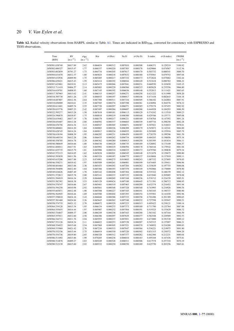
20 V. Van Eylen et al.

Table A2. Radial velocity observations from HARPS, similar to Table A1. Times are indicated in BJDTDB, converted for consistency with ESPRESSO andTESS observations.

Time RV 𝜎RV H𝛼 𝜎(H𝛼) Na D 𝜎(Na D) S-index 𝜎(S-index) FWHM[BJD] [m s−1] [m s−1] [m s−1]

2458501.638740 26817.89 2.62 0.064654 0.000312 0.007010 0.000308 0.606371 0.129219 3100.922458502.606327 26815.47 1.77 0.066337 0.000220 0.007383 0.000178 0.629866 0.074567 3112.362458503.602859 26791.27 1.73 0.064734 0.000205 0.007617 0.000170 0.503732 0.088541 3089.702458504.631670 26812.37 1.80 0.065824 0.000218 0.007632 0.000180 0.570561 0.079752 3097.042458505.632936 26809.90 1.75 0.065485 0.000217 0.007332 0.000173 0.572624 0.075682 3102.442458506.629421 26815.43 1.59 0.065414 0.000192 0.006944 0.000149 0.521618 0.090782 3096.222458507.623881 26819.91 2.13 0.065475 0.000266 0.007041 0.000231 0.660550 0.103650 3105.152458515.711419 26804.57 2.14 0.065083 0.000229 0.006566 0.000215 0.805628 0.235556 3066.802458516.619701 26808.93 1.60 0.067145 0.000192 0.006836 0.000148 0.552813 0.111421 3083.652458517.707965 26813.62 2.41 0.066315 0.000257 0.006271 0.000258 0.421222 0.311990 3058.202458518.595738 26811.26 1.55 0.066935 0.000197 0.006917 0.000146 0.471438 0.082643 3104.182458518.687807 26812.36 2.64 0.067388 0.000311 0.007334 0.000305 0.366182 0.242884 3087.912458519.656909 26810.61 2.35 0.067585 0.000274 0.007298 0.000261 0.436994 0.204376 3078.222458520.611601 26805.74 2.55 0.067720 0.000297 0.006571 0.000285 0.379174 0.197455 3082.922458520.633776 26807.23 2.42 0.067497 0.000284 0.006697 0.000268 0.444928 0.184293 3086.502458522.595277 26813.28 1.50 0.067618 0.000181 0.006113 0.000129 0.374242 0.113518 3089.232458524.596870 26818.87 1.75 0.068818 0.000219 0.006300 0.000168 0.429766 0.135771 3085.082458524.619462 26817.19 1.78 0.068179 0.000217 0.006221 0.000169 0.536764 0.147592 3091.242458528.654407 26812.28 2.88 0.068592 0.000337 0.006683 0.000339 0.407716 0.298258 3082.282458528.676756 26814.34 3.13 0.068547 0.000365 0.006871 0.000387 0.307021 0.316033 3078.012458530.606801 26814.20 1.84 0.069083 0.000226 0.006309 0.000179 0.545872 0.142241 3084.002458530.628745 26814.24 1.84 0.069017 0.000224 0.006935 0.000181 0.503089 0.155916 3085.792458538.618194 26808.39 1.95 0.066202 0.000231 0.006459 0.000195 0.728370 0.199296 3081.592458538.640334 26812.28 2.06 0.066435 0.000242 0.006734 0.000209 0.484243 0.198056 3075.342458540.558705 26814.78 2.29 0.066362 0.000280 0.006913 0.000250 0.303395 0.181834 3084.112458540.580649 26816.66 1.88 0.066530 0.000229 0.006735 0.000189 0.528892 0.173109 3086.572458541.604011 26817.91 1.83 0.065992 0.000219 0.006594 0.000178 0.760144 0.179542 3081.042458541.625735 26815.79 1.81 0.065906 0.000210 0.006525 0.000172 0.679760 0.190828 3079.242458543.572115 26814.05 1.62 0.065838 0.000201 0.006545 0.000148 0.512478 0.129675 3090.802458543.593839 26811.56 1.56 0.065324 0.000187 0.006775 0.000137 0.618684 0.137910 3089.112458545.615206 26817.88 2.23 0.074901 0.000275 0.010693 0.000243 1.087332 0.237695 3078.052458546.558271 26819.42 1.97 0.065589 0.000241 0.006981 0.000199 0.674405 0.159411 3096.962458548.601664 26813.88 2.38 0.065453 0.000292 0.007284 0.000262 0.335639 0.197755 3086.082458549.594890 26812.40 1.64 0.065366 0.000193 0.007379 0.000149 0.592066 0.170009 3078.902458549.616626 26807.49 1.78 0.065142 0.000208 0.007304 0.000168 0.535322 0.188159 3082.122458551.572813 26815.78 2.00 0.065141 0.000233 0.007152 0.000196 0.633940 0.205005 3078.082458551.594919 26816.34 2.29 0.064669 0.000265 0.007168 0.000236 0.576712 0.224159 3085.512458553.582392 26816.38 3.53 0.065129 0.000424 0.007189 0.000445 0.711391 0.296712 3096.952458554.570747 26816.66 2.67 0.065401 0.000319 0.007463 0.000299 0.632174 0.216452 3091.942458554.594230 26810.98 2.92 0.065041 0.000348 0.007328 0.000340 0.743993 0.234926 3090.762458555.603071 26812.48 1.98 0.065508 0.000227 0.007183 0.000191 0.565103 0.190737 3080.902458556.564945 26816.44 1.69 0.065580 0.000202 0.007293 0.000154 0.555501 0.141030 3092.962458557.558810 26824.16 2.43 0.066040 0.000288 0.007333 0.000258 0.701496 0.201289 3090.652458557.581460 26824.84 2.26 0.065645 0.000262 0.007248 0.000232 0.727598 0.193947 3090.212458558.574735 26821.12 2.78 0.066872 0.000329 0.007223 0.000313 0.495422 0.238121 3100.142458564.534128 26813.34 1.95 0.066154 0.000233 0.007373 0.000189 0.711700 0.153764 3087.062458564.555655 26814.44 1.97 0.065907 0.000232 0.007504 0.000191 0.519325 0.153629 3086.722458565.534847 26809.37 2.06 0.066249 0.000238 0.007443 0.000200 2.563182 0.187104 3084.592458565.557011 26812.60 2.58 0.066306 0.000297 0.007829 0.000277 0.582548 0.229589 3092.532458566.544711 26811.76 2.04 0.065955 0.000237 0.007051 0.000193 0.473000 0.191530 3089.122458567.531126 26818.34 2.11 0.066022 0.000253 0.007158 0.000207 0.545315 0.157097 3086.212458568.554022 26815.68 2.54 0.067969 0.000305 0.007521 0.000270 0.740052 0.216288 3090.832458569.533969 26821.42 2.78 0.067216 0.000333 0.007047 0.000304 0.536221 0.219075 3091.802458570.532156 26815.44 2.75 0.066919 0.000330 0.007220 0.000302 0.831315 0.230372 3094.292458570.554736 26819.80 2.65 0.066328 0.000312 0.007377 0.000282 0.842366 0.212231 3080.042458586.511092 26813.86 1.99 0.070205 0.000238 0.006010 0.000183 0.495104 0.167436 3075.812458588.514878 26809.27 2.83 0.069249 0.000328 0.006511 0.000306 0.617578 0.257318 3070.192458590.512139 26815.60 2.03 0.069332 0.000230 0.006550 0.000189 0.625750 0.203256 3065.81

MNRAS 000, 1–?? (0000)

21

Table A3. Joint transit and RV model priors. Values and the choice of prior is described in more detail in Section 4. A Normal distribution with mean ` andstandard deviation 𝜎 is indicated as N(`, 𝜎) . A Bounded Normal distribution, truncated by a lower limit 𝑙 and an upper limit 𝑢 is indicated as BN(`, 𝜎; 𝑙, 𝑢) .A uniform distribution with lower limit 𝑙 and upper limit 𝑢 is indicated by U(𝑙, 𝑢) . A Beta distribution with parameters 𝑎 and 𝑏 is indicated with B(𝑎, 𝑏) , ifit is further bound by a lower limit 𝑙 and upper limit 𝑢, it is indicated as BB(𝑎, 𝑏; 𝑙, 𝑢) .

Description Parameter Unit Prior

Stellar mass 𝑀★ (𝑀� ) BN(0.386, 0.008; 0, 3)Stellar radius 𝑅★ (𝑅� ) BN(0.378, 0.011; 0, 3)Limb darkening 𝑞1 U(0, 1)Limb darkening 𝑞2 U(0, 1)Orbital period (b) 𝑃𝑏 days U(3.35, 3.37)Orbital period (c) 𝑃𝑐 days U(5.65, 5.67)Orbital period (d) 𝑃𝑑 days U(11.37, 11.39)Time of conjunction (b) 𝑡c,b (BJDTDB − 2458387) U(0.04, 0.14)Time of conjunction (c) 𝑡c,c (BJDTDB − 2458387) U(2.45, 2.55)Time of conjunction (d) 𝑡c,d (BJDTDB − 2458387) U(2.63, 2.73)Eccentricity (b) 𝑒b BB(1.52, 29.0; 0, 1)Eccentricity (c) 𝑒c BB(1.52, 29.0; 0, 1)Eccentricity (d) 𝑒d BB(1.52, 29.0; 0, 1)Argument of pericenter (b) 𝜔b rad U(−𝜋, 𝜋)Argument of pericenter (c) 𝜔c rad U(−𝜋, 𝜋)Argument of pericenter (d) 𝜔d rad U(−𝜋, 𝜋)Planet mass (b) 𝑀p,b 𝑀⊕ N(2, 10)Planet mass (c) 𝑀p,c 𝑀⊕ N(7, 10)Planet mass (d) 𝑀p,d 𝑀⊕ N(3.5, 10)Planet radius (b) 𝑅p,b 𝑅⊕ N(0.0123, 10)Planet radius (c) 𝑅p,c 𝑅⊕ N(0.0231, 10)Planet radius (d) 𝑅p,d 𝑅⊕ N(0.0190, 10)Impact parameter (b) 𝑏𝑏 U(0, 1)Impact parameter (c) 𝑏𝑐 U(0, 1)Impact parameter (d) 𝑏𝑑 U(0, 1)Mean flux mf N(0, 10)Log photometric jitter log 𝜎phot N(2, 100)Offset HARPS 𝛾harps m s−1 N(0, 10)Offset ESPRESSO 𝛾espresso m s−1 N(0, 10)Log jitter HARPS log 𝜎2,rv,HARPS m s−1 N(log(1) , 5)Log jitter ESPRESSO log 𝜎2,rv,ESPRESSO m s−1 N(log(1) , 5)Photometry hyperparameter log 𝑆0 N(log(𝜎2

phot) , 10)Photometry hyperparameter log 𝛼0 N(log(2𝜋/10) , 10)RV hyperparameter log 𝑆1 N(log(5) , 2)RV hyperparameter log 𝛼1 N(log(2𝜋/50) , 2)RV hyperparameter log𝑄 N(log(5) , 2)

MNRAS 000, 1–?? (0000)

22 V. Van Eylen et al.

Table A4. Small planets (𝑅 < 3 𝑅⊕) with well-measured masses (< 20%) and radii (< 20%) orbiting M dwarf (𝑇eff < 4000 𝐾 ) stars. For each system, thesource of the planet discovery and of each parameter is listed. Some uncertainties were symmetrised for simplicity.

Notes. (a) Luque et al. (2019); (b) Berta-Thompson et al. (2015); (c) Bonfils et al. (2018); (d) Charbonneau et al. (2009); (e) Harpsøe et al. (2013); (f) Kemmer et al. (2020); (g) Crossfield et al. (2015);(h) Kosiarek et al. (2019); (i) Damasso et al. (2018); (j) Montet et al. (2015); (k) Benneke et al. (2019); (l) Hirano et al. (2018); (m) Hamann et al. (2019); (n) Steffen et al. (2012); (o) Jontof-Hutter et al. (2016);

(p) Astudillo-Defru et al. (2020); (q) Kostov et al. (2019); (r) Cloutier et al. (2019); (s) Dittmann et al. (2017); (t) Lillo-Box et al. (2020); (u) Cloutier et al. (2020a);(v) Cloutier et al. (2020b); (w) Gillon et al. (2016); (z) Gillon et al. (2017); (y) Grimm et al. (2018); (z) This work.

System Disc. Period Ref. Radius Ref. Mass Ref. Density Ref. Mstar Ref. Rstar Ref.[d] [R⊕ ] [M⊕ ] [g cm−3] [M� ] [R� ]

GJ 357 b (a) 3.93072 ± 0.00008 (a) 1.217 ± 0.084 (a) 1.84 ± 0.31 (a) 5.6 ± 1.5 (a) 0.342 ± 0.011 (a) 0.337 ± 0.015 (a)GJ 1132 b (b) 1.628931 ± 0.000027 (c) 1.13 ± 0.056 (c) 1.66 ± 0.23 (c) 6.3 ± 1.3 (c) 0.181 ± 0.019 (c) 0.2105 ± 0.0094 (c)GJ 1214 b (d) 1.58040456 ± 0.00000016 (e) 2.85 ± 0.2 (e) 6.26 ± 0.86 (e) 1.49 ± 0.33 (e) 0.15 ± 0.011 (e) 0.216 ± 0.012 (e)GJ 3473 b (f) 1.1980035 ± 0.0000018 (f) 1.264 ± 0.05 (f) 1.86 ± 0.3 (f) 5.03 ± 1 (f) 0.36 ± 0.016 (f) 0.364 ± 0.016 (f)K2-3 b (g) 10.054626 ± 0.000011 (h) 2.29 ± 0.23 (i) 6.48 ± 0.96 (h) 3.7 ± 1.38 (h) 0.601 ± 0.089 (h) 0.561 ± 0.068 (h)K2-18 b (j) 32.940045 ± 0.00001 (k) 2.61 ± 0.087 (k) 8.63 ± 1.35 (k) 2.67 ± 0.5 (k) 0.4951 ± 0.0043 (k) 0.4445 ± 0.0148 (k)K2-146 b (l) 2.6446 ± 0.00006 (m) 2.05 ± 0.06 (m) 5.77 ± 0.18 (m) 3.69 ± 0.21 (m) 0.331 ± 0.009 (m) 0.33 ± 0.01 (m)K2-146 c (m) 4.00498 ± 0.00011 (m) 2.16 ± 0.07 (m) 7.49 ± 0.24 (m) 3.92 ± 0.27 (m) 0.331 ± 0.009 (m) 0.33 ± 0.01 (m)Kepler-26 b (n) 12.28 ± 0.0003 (o) 2.78 ± 0.11 (o) 5.12 ± 0.63 (o) 1.26 ± 0.2 (o) 0.544 ± 0.025 (o) 0.512 ± 0.017 (o)Kepler-26 c (n) 17.2559 ± 0.0006 (o) 2.72 ± 0.12 (o) 6.2 ± 0.65 (o) 1.61 ± 0.25 (o) 0.544 ± 0.025 (o) 0.512 ± 0.017 (o)L168-9 b (p) 1.4015 ± 0.00018 (p) 1.39 ± 0.09 (p) 4.6 ± 0.56 (p) 9.6 ± 2.1 (p) 0.62 ± 0.03 (p) 0.6 ± 0.022 (p)L98-59 c (q) 3.6904 ± 0.0003 (r) 1.35 ± 0.07 (r) 2.42 ± 0.35 (r) 5.4 ± 1.2 (r) 0.312 ± 0.031 (r) 0.314 ± 0.014 (r)LHS 1140 b (s) 24.73694 ± 0.00041 (t) 1.635 ± 0.046 (t) 6.38 ± 0.45 (t) 8.04 ± 0.82 (t) 0.191 ± 0.012 (t) 0.2134 ± 0.0035 (t)LHS 1140 c (s) 3.777929 ± 0.00003 (t) 1.169 ± 0.038 (t) 1.76 ± 0.17 (t) 6.07 ± 0.78 (t) 0.191 ± 0.012 (t) 0.2134 ± 0.0035 (t)LTT 3780 b (u) 0.768448 ± 0.000055 (u) 1.332 ± 0.074 (u) 2.62 ± 0.47 (u) 6.1 ± 1.7 (u) 0.401 ± 0.012 (u) 0.374 ± 0.011 (u)LTT 3780 c (u) 12.2519 ± 0.003 (u) 2.3 ± 0.16 (u) 8.6 ± 1.45 (u) 3.9 ± 1 (u) 0.401 ± 0.012 (u) 0.374 ± 0.011 (u)TOI-1235 b (z) 3.444729 ± 0.000031 (z) 1.738 ± 0.083 (z) 6.91 ± 0.8 (z) 7.4 ± 1.4 (z) 0.64 ± 0.016 (z) 0.63 ± 0.015 (z)TRAPPIST-1 b (w) 1.51087081 ± 0.0000006 (x) 1.121 ± 0.031 (y) 1.017 ± 0.149 (y) 0.963 ± 0.122 (y) 0.089 ± 0.007 (y) 0.117 ± 0.0036 (x)TRAPPIST-1 c (w) 2.4218233 ± 0.0000017 (x) 1.095 ± 0.03 (y) 1.156 ± 0.136 (y) 1.17 ± 0.11 (y) 0.089 ± 0.007 (y) 0.117 ± 0.0036 (x)TRAPPIST-1 d (w) 4.04961 ± 0.000063 (x) 0.784 ± 0.023 (y) 0.297 ± 0.037 (y) 0.817 ± 0.086 (y) 0.089 ± 0.007 (y) 0.117 ± 0.0036 (x)TRAPPIST-1 e (w) 6.099615 ± 0.000011 (x) 0.91 ± 0.026 (y) 0.772 ± 0.077 (y) 1.358 ± 0.097 (y) 0.089 ± 0.007 (y) 0.117 ± 0.0036 (x)TRAPPIST-1 f (w) 9.20669 ± 0.000015 (x) 1.046 ± 0.029 (y) 0.934 ± 0.079 (y) 1.08 ± 0.05 (y) 0.089 ± 0.007 (y) 0.117 ± 0.0036 (x)TRAPPIST-1 g (w) 12.35294 ± 0.00012 (x) 1.148 ± 0.032 (y) 1.148 ± 0.097 (y) 1.01 ± 0.05 (y) 0.089 ± 0.007 (y) 0.117 ± 0.0036 (x)TRAPPIST-1 h (w) 18.767 ± 0.004 (x) 0.773 ± 0.026 (y) 0.331 ± 0.053 (y) 0.954 ± 0.15 (y) 0.089 ± 0.007 (y) 0.117 ± 0.0036 (x)L231-32 b (z) 3.3601538 ± 0.0000048 (z) 1.206 ± 0.039 (z) 1.58 ± 0.26 (z) 4.97 ± 0.94 (z) 0.386 ± 0.008 (z) 0.378 ± 0.011 (z)L231-32 c (z) 5.6605731 ± 0.0000031 (z) 2.355 ± 0.064 (z) 6.15 ± 0.37 (z) 2.60 ± 0.26 (z) 0.386 ± 0.008 (z) 0.378 ± 0.011 (z)L231-32 d (z) 11.379573 ± 0.000013 (z) 2.133 ± 0.058 (z) 4.78 ± 0.43 (z) 2.72 ± 0.33 (z) 0.386 ± 0.008 (z) 0.378 ± 0.011 (z)

MNRAS 000, 1–?? (0000)