mass balance models of ekman transport and nutrientfluxes ... · global biogeochem!cal cycles, vol....

GLOBAL BIOGEOCHEM!CAL CYCLES, VOL. 8, NO. 2, PAGES 165-177, JUNE 1994

Mass balance models of Ekman transport and nutrient fluxes in coastal upwelling zones

Paul W. Jewell

Department of Geology and Geophysics, University of Utah, Salt Lake City

Abstract. The nutrient cycles of coastal upwelling zones are studied with simple mass balance models of Ekman transport, longshore transport, surface productivity, and dissolved phosphorous. The models are constrained with data from the Peru, northwest Africa, and Oregon upwelling systems. The onshore-offshore mass balance model agrees with published Ekman transport, surface productivity, and nutrient data as well as hypothesized nutrient f-ratios for highly productive coastal settings. The onshore-offshore model suggests that increased primary productivity in glacial-era coastal upwelling zones was not a linear function of Ekman transport, but instead was probably dependent on the physical and chemical dynamics of a specific setting. In the Peru upwelling system, longshore equatorward surface currents and poleward undercurrents produce positive surface nutrient gradients in the equatorward direction and relatively constant gradients in subsurface waters. Longshore nutrient gradients off northwest Africa are positive in the equatorward direction for both surface and subsurface waters. These observations are consistent with the conceptual model of surface and subsurface currents which are moving toward the equator and continually being upgraded by the offshore flux of nutrients. The northwest Africa and Peru data are not consistent with the longshore nutrient model of Redfield et al. (1963).

Introduction

Understanding exchanges of nutrients and oxygen between various parts of the ocean and the atmosphere has occupied the imagination of oceanographers and earth scientists for decades [e.g., Broecker, 1974; Garrels and Perry, 1974; Holland, 1978; Berner et al., 1983]. Mass balance models of biogeochemical constituents have prov- en to be effective tools for understanding these exchanges in both modem and ancient settings [e.g. $armiento et al., 1988; Shaffer, 1989]. Other models have addressed the cause of atmospheric CO2 changes within the context of circulation in the ocean [e.g. Ennever and McElroy, 1985; Toggweiler and $armiento, 1985; Wenk and $ie- genthaler, 1985]. While these models have been useful in testing various scenarios of world ocean processes, they have (almost by necessity) neglected the details of the margins of ocean basins. Coastal upwelling zones are among the most biologically productive areas of the ocean [Koblents-Mishke, 1970; Berger, 1989] and thus are critical to understanding these marginal settings. Very few biogeochemical models of coastal upwelling have been attempted. A notable exception is the work of RedfieM et at. [ 1963].

A considerable body of literature also addresses the r,,1,• that ,,,,w•n•,o may have played in global processes. Newell et al. [1978] were the first to suggest that in-

Copyright 1994 by the American Geophysical Union

Paper number 94GB00097 0886-6236/94/94GB-00097510.00

creased low-latitude upwelling during a glacial climate may have produced lower atmospheric CO 2. Boyle [1986] presents a box model which suggests that increased low-latitude upwelling lowered atmospheric CO 2 by-25 parts per million by volume. The rain ratio theory [Berger and Keir, 1984] holds that increased Ek- man transport during glacial times decreased atmospheric CO 2 due to the very high organic carbon/carbonate carbon ratios which are typical of upwelling zones. $arnthein et al. [1988] summarize palcoproductivity relationships of the low- and mid-latitude oceans and how they may have influenced atmospheric CO 2.

Discussions of low-latitude upwelling during glacial periods implicitly assume that stronger zonal winds increased Ekman transport along coastal margins or Ekman pumping near the equator. This in turn increased surface productivity thereby decreasing atmospheric CO2. All of these assumptions merit examination within the frame- work of modem meteorological and oceanographic data. For instance, although it is recognized that stronger winds generally cause higher Ekman transport [e.g., Smith, 1981; Lentz, 1992], there are dynamic situations such as the western coast of Australia where equatorward winds result in little or no Ekman transport [Smith et al., 1991]. On the other hand, the commonly assumed link between strong Ekman transport and high surface productivity has not been critically examined with data from modem coastal upwelling zones.

The present study was undertaken to provide a quantita- tive understanding of the relationships between Ekman transport, longshore currents, surface productivity, and

166 JEWELL: COASTAL UPWELLING MODELS

nutrient concentrations in coastal upwelling zones. The procedure involves constructing simple, mass balance models of idealizeA coastal upwelling. Chemical data bases from well-studied modem oceanographic settings then constrain results of the mass balance models. The

study is meant to address several questions. (1) Are the relationships between productivity, Ekman transport, and nutrient flux consistent between upwelling zones in wide- ly different settings? (2) Can the longshore model of RedfieM et al. [1963] be validated by field data and used to explain the development of oxygen depletion and nutrient enrichment in water over continental shelves? (3) What implications might these simple mass balance models have for upwelling systems in the geologic past? Al- though not specifically addressed by this study, the procedure is applicable to equatorial upwelling as well as coastal upwelling.

Models of Modern Coastal Upwelling

The general physical, biological, and chemical processes in modern coastal upwelling zones are agreed upon by most researchers [e.g. Richards, 1981]. Upwelling occurs along the eastern borders of ocean basins (i.e., the western edges of continents) where winds are equatorward. These equatorward geostrophic winds are the result of quasi-stationary, high-pressure atmospheric cells in the middle of the ocean. In the modem ocean, coastal upwelling is most intense along the coasts of northwest Africa, southwest Africa, Peru-Chile, and the west coast of the United States. Seasonal upwelling occurs in various parts of the Indian Ocean. Palcogeographic reconstructions in conjunction with the placement of atmospheric high- and low-pressure cells have allowed zones of coastal upwelling to be pinpointed in palcogeographic reconstructions [e.g. Parrish, 1982].

The equatorward winds in a coastal upwelling system produce a surface shear stress which is balanced by Co- riolis forces. The resulting flow is perpendicular to the wind direction. The total amount of mass transport (termed Ekman transport) is equal to x/f where x is the wind shear stress andf is the Coriolis parameter. Surface Ekman transport occurs in a relatively shallow (order of tens of meters) zone near the surface. The thickness of the Ekman layer is a function of the density stratification, the Coriolis parameter, and the shear stress in the fluid and can vary significantly from one upwelling system to the next [Smith, 1981; Lentz, 1992].

The offshore movement of water due to Ekman transport is balanced by the onshore transport of water beneath the surface Ekman layer. Upwelled water is generated within 100-300 m of the surface [Bowden, 1983; Pond and Pick- ard, 1983] and generally flows upward over the continental shelf and/or shelf break. The effect of the

upwelling process is to cause isopycnals to intersect the water surface adjacent to a landmass (Figure 1). The dense, nutrient-rich water enhances surface productivity adjacent to the coast. The level of surface productivity is usually greatest near the coastline and decreases seaward. The highest concentration of biologically produced mate- rials such as chlorophyll is located seaward of the zone in which isopycnal surfaces intersect the water surface [Friebertshauser et al., 1975; Hafferty et al., 1978] (Figure 1). The enhanced surface productivity of upwelling zones increases biological activity at other trophic levels as well as the flux of organic matter from the surface photic zone.

A fraction of organic matter produced at the surface sinks through the photic zone and is remineralized at depth by a variety of oxidants. Beneath the photic zone of upwelling systems, oxygen, and more rarely, nitrate are consumed. In rare instances in the Pacific, sulfate reduction has been observed [Dugdale et al., 1977]. Bar-

100

200

300 i i

offshore Ekman ,,•_••productive photic ._• I aye r zone

,•. • ...::?•

I I I•"•-.., I I I I •ii!:' I

100

200

300

PO 4 (/• mot/L)

I I

Figure 1. Cross-sectional hydrographic plots near 15øS off of the Peru coast. JOINT II expedition, May 5-6, 1977 [Hafferty et al., 1978].

From stations 363-377,

JEWELL: COASTAL UPWELLING MODELS 167

ber and Smith [1981] attribute this to strong poleward undercurrents which, according to the longshore nutrient model of RedfieM et al. [1963], lead to enhanced subsurface nutrient enrichment and oxygen depletion.

Model Formulation

Actual coastal upwelling zones are a combination of both longshore and onshore-offshore processes. In this study, simple models of both dimensions have been con- stmcted in order to highlight the characteristic processes of each.

Onshore-offshore model. Onshore-offshore coastal

upwelling is parameterized as a two-dimensional box model which represents the general physical and chemical features of upwelling zones (Figures 1 and 2). Two offshore boxes are connected to onshore boxes (Figure 2). The offshore boxes serve as boundary conditions for variables of the nearshore boxes. The boundary between nearshore and offshore boxes is arbitrary. In reality there is a continuous gradation of chemical properties in the cross-shelf direction (Figure 1). The box model represents property gradients such as primary productivity and nutrient concentration as discrete values.

The four boxes form a continuous loop which exchanges water via Ekman transport, T (Figure 2). Ekman volume transport has units of m2/s, that is, volume flux per unit distance of shoreline. Ekman transport can be calculated as (1) surface wind shear stress divided by the Coriolis parameter and water density, (2) offshore velocity inte- grated over the surface Ekman layer depth, or (3) onshore mass transport below the surface Ekman layer. Compari- son of these methods for calculating Ekman transport in a variety of settings is given Smith [1981] and Lentz[1992]. Integration over the surface Ekman layer is employed in this paper because, unl•e wind shear calculations, water transport is most directly related to nutrient concentrations of the box model. Furthermore, surface offshore transport is more coherent than onshore transport which often interacts with the bottom boundary layer of the continental shelf.

Onshore-offshore gradients in wind shear magnitude are documented in many coastal upwelling regions [e.g. Ba- kun and Nelson, 1991] and may account for the observed onshore-offshore variability in surface Ekman transport rates [Lentz, 1992]. The influence of wind stress gradi-

ents is not evaluated in this study, and Ekman transport in the box model is assumed to be constant.

The subsurface coastal (sc) zone receives water from the subsurface offshore (so) zone (Figure 2). Although the specifics of individual upwelling systems vary, the sc zone probably extends from 30-200 m depth, depending on location of the upwelling relative to the continental shelf. The productive photic zone (pzp) receives water from the underlying sc box and is separated from it by upward curving isopycnal surfaces (Figure 1). The pzp box probably extends from the surface to 20-50 m depth. The highest biological productivities of coastal upwelling zones take place in the pzp box.

Estimates of primary productivity in upwelling photic zones are relatively numerous. Much less is known about how much of this productivity leaves the photic zone [e.g. Berger et al., 1989]. Here the amount of primary productivity P exported to the sc box is multiplied by the factor 0•. The flux of organic material to water below the sc box and to the sediments is represented by 0%. The remaining fraction of biogenic particles produced in the productive photic zone (0•) is advected offshore.

Model primary productivity P has units of moles m '• s '• and must be converted to values commonly reported for surface productivity (usually g (2 m '2 yr'•). Assuming a C:P ratio of 106, it can be found that 1 g C m -2 yr '• = 2.5 x 10 's mmoles P m '2 s '•. Multiplying this figure by the width of the productive photic zone gives the net biogenic particle flux for the model.

The pzp box can have an arbitrary width. Widths cho- sen for this study correspond to published, spatially averaged values of surface productivity (Table 1). The arbitrary width does not change the model results since the units employed in the model (i.e., cross-shelf nutrient gradients and productivity) are internally consistent. For instance, a wider pzp box will lead to higher values of P which in turn makes computed cross-shelf property differences higher.

Mass balance equations which relate the flux of chemical components between the model boxes are constructed in a fashion similar to those outlined in other studies

[e.g., Broecker, 1974]. In theory, a number of chemical tracers could be used in a mass balance model such as this

one. In reality, only databases of the common nutrients and oxygen are sufficiently detailed to provide the com-

Offshore EkrnonLover !., T IProduct•ve Photic Zone./ff T// / /

mhermocl ins .......... -•-- •- ......... / /

,• . . ' • •t (.•uDsurtoce •oostol •one/

•nsn• )c over a ,'cP • Csc ) / •x •

F•ure 2. Box model represenUtion of coasUl upwe•g. Symbols are expla• • the text.

168 JEWELL.' COASTAL UPWELLING MODELS

Table 1. Description of Variables Used to Constrain the Upwelling Box Model

Peru Northwest Africa Oregon

Location 15øS 21ø40'N 45 ø N

Oceanographic expedition JOINT II JOINT I CUE II

Date March-May 1977 March-April 1974 July-August, 1973

Width of productive zone, km

Primary productivity, gC m'2 yr 4

Depth of surface Ekman layer, m

Surface Ekman transport, m2/s

20, 40 • 50 b Variable

1400 • 720 b 250 ½

30 a 35 a 20 a

0.82 + 1.48 a 1.45 + 1.84 a 0.65+ 1.09 0.71 + 0.96 ß 0.82 + 0.791 0.25 + 0.41

Depth of onshore flow, m 90 ½ 40 ½ 60 ½

' Packard et al. [1983]. • Huntsman and Barber [1977]. c Walsh [1981]. Reported value does not correspond to the July-August 1973 time period. d Smith [1981]. c Lentz [1992]; calculated from thickness of the surface mixed layer plus a transition that is half the thickness of the surface mixed layer. tBaden_Dangon et al. [1986]

parisons necessary to constrain models of coastal upwelling.

A simple model of biological particle flux using PO n as the master variable is employed in this study. The multi- ple nitrogen compounds present in some coastal upwelling environments (e.g., NO3, NO2, NHn) make this a more difficult element to model. Oxygen could also be modeled if exchange with the atmosphere were taken into account. Modeling oxygen concentrations, however, is complicated by nitrate reduction in the deep water of low-oxygen systems.

The mass balance equation for POn in the pzp box is (Figure 2):

P 0 4 , t,zt, - P 0 4 , sc p =--- (1) Ax T

The PO n mass balance equation in subsurface coastal (so) box is:

P04, sc- P04, so P' Otsc = (2) Ax T

Longshore model. The longshore variability of nutrient elements in coastal settings was considered in the

classic paper by Redfield et al. [1963]. These authors argued that the longshore distribution of nutrients in a two-layer coastal system could be modeled as a balance between horizontal advection, vertical diffusion, and nutrient fluxes. In the upper layer these balances are [RedfieM et al. 1963, equation (5a)]:

dNv =-R + A dN w.f (3) V u is the mean velocity of the upper layer, R is loss of the nutrient N by photosynthesis, h is depth of the upper layer, and A is vertical eddy diffusivity. The y coordinate is assumed to be in the longshore direction. A similar expression can be constructed for the lower layer [RedfieM et al., 1963, equation (Sb)]:

Vr . dNr = R- A dN ay h az (4) If one assumes that the upper and lower layers are of equal thickness and that the loss of nutrients due to photosynthesis in the upper layer is exactly balanced by respiration in the lower layer, then these two equations can be combined to yield:


dN• Vv dNv - (5)

Equation (5) shows that if the upper and lower velocity have opposite signs (a common situation in upwelling zones in which equatorward, wind-driven surface currents overlie poleward undercurrents) then the horizontal nutrient gradients in the two layers will both decrease in the equatorward direction [RedfieM et al. 1963].

More detailed versions of (3) and (4) can be derived by assuming that the depths and biogenic fluxes in the two layers are not equal:

dNv dN hr. Vv . ---- =-hr. Rv +A (6)

dNœ AdN h• . V• . -• = h• . R•- dz (7)

Equations (6) and (7) can be combined to yield:

dNr hvVv dNv (hvRv- hrRD - - (8)

dy h r Vr dy h r Vr

By assuming that (1) Tv = hv Vv and Tt• = hL VL represent two-dimensional, longshore transport in the upper and lower layers, respectively, and (2) only a fraction of surface productivity ({x•) is remineralized in the lower layer, (8) can be recast into the same terms used in the cross- shelf box model (equations 1 and 2):

l•P04, sc TU l•P04, pzp (hr. P-hr. Ctsc . P) Ay = -'•-• ' Ay - T• (9)

Field settings

Constraints on the physical and chemical dynamics of the cross-shelf and longshore models are considered within the context of data from three field settings: the Peru system near 15øS, the northwest Africa system at 21ø40'N, and the Oregon system at 45øN. The use of these settings is motivated by several considerations. All three localities were studied exhaustively in the mid-1970s by research groups which used similar tech- niques to determine surface productivity, Ekman transport, and nutrient concentrations. A certain degree of confidence can therefore be drawn in the comparisons of the three settings. On the other hand, the three systems have different source-water chemistry and bathymetry and thus represent the significant contrasts which can occur in coastal upwelling. Finally, published summaries of Ek- man transport and surface productivity over periods of approximately tw'o months are available, thereby eliminating much of the high-frequency noise inherent in short-term coastal upwelling studies.

Peru. Coastal upwelling occurs off the coast of Peru between 6 ø and 17 ø S in response to the southeast trade winds of the low-latitude, southern hemisphere. Below

the surface Ekman layer, longshore transport is domi- nated by the poleward Chile-Peru Undercurrent which is the source for most of the upwelled water [e.g. Brock- mann et al., 1980]. This current is derived from the Pacific Equatorial Undercurrent. Equatorial upwelling produces nutrient-rich, oxygen-deficient water which in turn influences intermediate-depth water characteristics from 5ø-16øS. The well-studied area near 15øS is charac-

terized by high surface productivities, bottom velocities which are close to zero, and organic carbon-rich bottom sediments [Suess et al., 1987]. The continental shelf near 15øS is relatively narrow (-20 km wide).

Offshore Ekman transport along a transect at 15øS was calculated to be 0.82 __+ 1.48 m2/s by Smith [1981] and 0.71 __+ 0.96 m2/s by Lentz [1992] from data collected during the JOINT-II oceanographic expedition in the spring of 1977. Onshore mass transport is roughly 50% higher than offshore transport [Smith, 1981]. The differ- ence is due to entrainment of a portion of the onshore flow in a longshore direction. At 15øS, offshore flow extends from the surface to 30 m depth, and onshore flow exists between 30-120 m depth (Figure 3). Equatorward flow is observed to depths of 30 m and the poleward undercurrent at depths between 30 and 120 m (Figure 3). In other words, the pzp and sc compartments of both the onshore-offshore and longshore box models have the same depths.

Primary productivity has been measured throughout the Peruvian upwelling system. A mean primary productivity of 400-700 g C m'2yr" for the entire system from 5ø-15øS has been suggested [$uess et al., 1987]. Produe- tivities are considered to be higher near 15øS. Using the JOINT II data, Packard et al. [ 1983] calculate an average productivity of- 1400 g C m'2yr 4 for the inner 40 km of the upwelling zone and somewhat less than half of that for the next 40 km seaward.

Northwest Africa. Along the northwest coast of Afri- ca, upwelling occurs throughout the year between 20 ø and 25 ø N latitude and seasonally over much wider latitudes [Futterer, 1983]. The data used here is from a transect at 21 ø 40' N near Cape Blanc collected during the JOINT I expedition in the spring of 1974 [Barber, 1977]. In this area, the continental shelf is -50 km wide. The highest values of surface productivity occur over the shelf. Al- though circulation along the shelf margin is spatially and temporally complex, the entire zone is characterized by an equatorward surface current (the Canary current). Poleward undercurrents occur over the inner continental

slope. Poleward undercurrents over the continental shelf are negligible and the entire flow regime over the continental shelf is 'equatorward [Smith, 1981] [Figure 3]. Offshore flow occurs to a depth of-35 m, and onshore velocity occurs between 35 m and 75 m depth [Smith, 1981]. These zones correspond to the p• and sc portions

cro•-•ad, and longshore •x -'- • • Huntsman and Barber [ 1977] report surface productivi-

ties of 1-3 g C m':d 4 over the continental shelf. An average primary productivity of 720 g C m'2yr 4 over a shelf width of 50 km is assumed for this study. MinaJ et al. [1986] argue that the productivity values of Huntsman


OREGON

5 JULY TO 28 AUGUST 1973

OFFSHORE 0

• •0 • 4O •. 60

c• 80

lOO 20 -

0 i

• 20 • 40 c• •0

c• 80 I

•oo_ -•o

NORTHWEST AFRICA PERU

I0 MARCH-6 APRIL 1974 22 MARCH-IO MAY 1977

ON SHOR E OFFSHORE ONSHORE OFF SHORE 0NS HORE

©ee•l I , , , 0 "•I ' ' ' 0 ' ' t'e• ' ' ' ß 20 20

', . I ß 40 ß ß 40

•e 60 ,- , • 60 i ' ' 0 • •0 ' 3'0 -10 10 20 3 0 80 -10 1 20 era/see 100

cm/sec -20 -10 0 10 20

POLEWARD EQUATORWARD POLEWARD EQUATORWARD

', ' ' •e 0 , , e• ,- 0 ' • ß 20 ' I I , ß 40 • 40 i

' ß 60 • ,lp I 60 , -10 0 10 20 30 40 80

ß I I • I cm/sec 100 0 10 20 30 40

era/see

cm/sec

POLEWARD EQUATORWARD

- leap e - ß ,,

- ß I - _ ß I _

I

I I I ß1 I I I - 20 - 10 0 10

cm/sec

Figure 3. Summary of longshore and offshore current meter data for northwest Africa, Peru, and Oregon [Smith, 1981].

20

and Barber [1977] are lower than typical productivities for northwest Africa. The Huntsman and Barber productivity values are used here because they correspond to the same time period of other measured properties (i.e., Ek- man transport and dissolved nutrient concentrations). Published values of surface Ekman transport during the JOINT I project are higher than those of the Peru upwelling system (Table 1).

Oregon. The Oregon upwelling system was analyzed in detail during the Coastal Upwelling Ecosystems (CUE II) program in 1973 (Table 1). Upwelling is most intense between late May and August [Small and Menzies, 1981]. Ekman transport is weaker than that of the Peru and Ore- gon systems (Figure 3, Table 1). There is a very strong longshore equatorial jet and relatively weak poleward undercurrent (Figure 3). Depths of the jet and undercurrent do not correspond to the depths of onshore and offshore transport.

Oregon upwelling productivity and nutrient databases for the period in which Ekman transport analyses were conducted are not as comprehensive as they are for Peru and northwest Africa. Much of the nutrient data collected

during July and August 1973 was at relatively shallow depths (Figure 3) [Stevenson et aL, 1975]. Furthermore, an average surface productivity for the July-August, 1973 time period has not been published. A general value of 250 g C m'2y& reported by Walsh [ 1981] for the Oregon system is used here.

Model results

Cross-shelf processes. Equations (1) and (2) can be combined to yield an expression which reflects the amount of phosphate consumed during the Ekman transport loop of the box model (Figure 2):

PO4, so-PO4,t,q, P- (1- asc) Ax T (lO)

The solution procedure for (10) involves calculating the amount of phosphate consumed during the Ekman transport loop for a number of stations from the JOINT I, JOINT II, and CUE II data sets. The availability of Ek- man transport, surface productivity, and nutrient data make (10) overdetermined. Extensive current meter and geochemical data allows Ekman transport [Smith, 1981; Lentz, 1992] and nutrient gradients (this study) to be determined with some degree of statistical confidence. Surface productivity, on the other hand, is generally reported as a single value [e.g., Walsh, 1981; Packard et al., 1983] although Huntsman and Barber [ 1977] report a range of surface productivities for northwest Africa.

A possible inconsistency in the cross-shelf box model is the choice of box model width. The width of the time-

averaged, nearshore surface productivity for Peru is 40 km [Packard et al., 1983], while the current meter moor- ing used to calculate Ekman transport was 15-20 km from shore [Smith, 1981; Lentz, 1992] (Figure 4). The Peru system cross-shelf box model was therefore evaluated for both 20-kin and 40-kin widths. Onshore-offshore nutri-

ent gradients in the Oregon system were evaluated at a variety of stations (and hence box model widths), because the nutrient database was so much smaller than that of the

Peru and northwest Africa systems. The irregularly spaced Oregon nutrient data was normalized to a 20 km box model width for the sake of comparison with the current meter station (Figure 4).

The amount of phosphate consumed in the Ekman transport loop (i.e., POn,,o - POn,•) shows considerable variability for all three upwelling systems (Figures 5, 6,


22ON .,

• \x • •'"?' "x \ ' :'.'..

\ • .:::..

ß .,oos ':'\... I ,' ':" ', ', "-, :-•'•.... '•.. I =.,o•o.- , ,, , ,..-':.

........ x. •--• •x •"' 90' 80ø 70ø 1000m loom

I ..•! ', -, x.:•: ,' !! ..':'.'.... 30 ø / !:.9' '?. •. • • -, -,... xL-•: '

\ '-,,\ •'.:.. 21000 ' .20 o lSo:•o'L -"' " .... "\-"'•'• .... ' !"':: '•:' / o 25 km -•,,, •c-.• •:: • ' ' ". "•.-'" / I - - ',,I ' ' - 0" "iJ '".

sow I $øE I I •'. 18 ø w 17.30' 17"00' 16"30'

,, I I .....::..:

'' " m ,OOm 50m •?: I 45ON _ 50 ø 200

/e ß //

•5'p ,J."• I // / / !•::-• J fi: /' / I " ,,o. ,•o. ,•. ,•o.w / ,

I• / / I 124030 ' 124øW

Figure 4. Location of stations for phosphate data (circles) and current meter data (triangles) used in the onshore-offshore box model analysis. Open circles for Peru refer to the inner shelf analysis (15-20 km offshore) whereas solid circles represent outer shelf (40-50 km) analysis.

lO lO

0.46-+ .38 Peru -20 km Peru-40 k m

0.84_+.34

o •////////////////• K".• •-///..•////'•. • , , 0.0 0.5 1.0 1.5 2.0 00.0 0.5 1.0 1.5 2.0 APO 4 (p. mol/L ) PO4(p. mol/L)

Figure 5. Histogram of calculated phosphate depletions in the Ekman transport loop for the Peru upwelling system.


10 •orthwest Africo

0.21_+ .10

00.0 0.2 0.4 PO4(mol/L)

Figure 6. Histogram of calculated phosphate depletions in the Ekman transport loop for the northwest Africa upwelling systems.

and 7). The Peru Ekman transport loop consumes 0.46 _.• 0.38 and 0.84 4- 0.34 pmol/L of POn for the 20-km and 40-km cross-shelf box model widths, respectively (Figure 5). The two-fold increase in the box model width and commensurate increase in calculated nutrient con-

sumption suggests that the cross-shelf box model is consistent. The phosphate consumed in the northwest Africa system (0.21 ñ 0.10 pmol/L for a 50 km wide model) is significantly less than that consumed in the Peru system (Figure 6). The Oregon system consumes a relatively high amount of nutrients in the Ekman transport loop

Oregon - 20 k m

O. 85 -+.59

øo.o 0.5 1.0 1.5 2.0

APO4(P. mol/L) Figure 7. Histogram of calculated phosphate depletions in the Ekman transport loop for the northwest Africa upwelling systems.

(0.86 __+ 0.59 •tmol/L), despite having relatively low surface productivity (Figure 7, Table 1).

The degree to which these geochemical data match productivity and Ekman transport data (Table 1) depends on the values of eta, that is the amount of surface productivity which is recycled in the shallow coastal layer (Figure 2). Choosing 0t• = 0.5 gives reasonable results for published values of Ekman transport in the Peru and northwest Africa systems, whereas et• = 0.25 gives the best results for Oregon (Table 2). The poorest fit between model and data is clearly the Oregon system, although as stated previously, the Oregon nutrient data are not as good as the Peru and northwest Africa data.

Two important points emerge from this analysis of productivity, Ekman transport and phosphate data in the cross-shelf domain of modern upwelling systems. (1) For a given value of 0•, the mass balance relationships be-

Table 2. Calculated Surface Ekman Transport Rates, T, in the Peru, Northwest Africa, and Oregon Upwelling Systems

Peru, Peru, Northwest Africa, Oregon, 20-km Width 40-km Width 50-km Width Variable Width

T, published 0.82 q- 1.48" 0.82 q- 1.48" 1.45 q- 1.84" 0.65 q, 1.09" 0.71 q- 0.96 •' 0.71 q- 0.96 •' 0.82 q- 0.79 ½ 0.25 q- 0.41 •'

T, calculated, o•: 0.75 0.83 2.13 0.07

T, calculated, 0t: 1.10 1.24 3.19 0.11

' Smith [1981].

b Lentz [1992]; calculated from thickness of the surfac• mixed layer plus a transition that is half the thickness of the surface mixed layer. c Baden-Dangon et al. [1986].

JEWELL: COASTAl., UPWELLING MODELS 173

tween Ekman transport, surface productivity, and nutrient consumption yield consistent results for three well-studied field areas with distinctly different bathymetries and source water chemistry. In the studies of Smith [1981] and Lentz [ 1992] as well as the box model calculations of Ekman transport using nutrient and surface productivity data (Table 2), northwest Africa has the highest, Peru the next highest, and Oregon the lowest Ekman transport rates. (2) The northwest Africa upwelling system has relatively low productivity and consumes the smallest amount of nutrients despite having the highest Ekman transport rate of the three systems.

The fraction of productivity remineralized in the sc box (oc•) plus the fraction escaping the Ekman loop (%) is crudely equal to the f ratio, that is, the ratio of new production to total production. For the Peru system, Suess [1980] estimated that 18 % of primary productivity sinks below 110 m. This roughly corresponds to oq of the box model (Figure 2). If so, then the f ratio of the box model is (% + 0c•) or 0.43-0.68 (Table 2). These values are consistent with f ratios reported for upwelling systems in general [Epply, 1989].

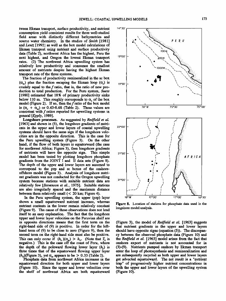
Longshore processes. As suggested by RedfieM et al. [ 1963] and shown in (5), the longshore gradients of nutrients in the upper and lower layers of coastal upwelling systems should have the same sign if the longshore velocities are in the opposite direction. This is the case for the Peru upwelling system (Figure 3). On the other hand, if the flow of both layers is equatorward (the case for northwest Africa; Figure 3), then longshore gradients of nutrients will have the opposite sign. This simple model has been tested by plotting longshore phosphate gradients from the JOINT I and II data sets (Figure 8). The depth of the upper and lower layers are assumed to correspond to the pzp and sc boxes of the onshore- offshore model (Figure 3). Analysis of longshore nutrient gradients was not conducted for the Oregon upwelling system because stations with suitable nutrient data are relatively few [Stevenson et al., 1975]. Suitable stations are also irregularly spaced and the maximum distance between them relatively small (< 20 kin; Figure 4).

In the Peru upwelling system, the upper (pzp) layer shows a small equatorward nutrient increase, whereas nutrient contents in the lower remain relatively constant (Figure 9). The cause of these observations does not lend itself to an easy explanation. The fact that the longshore upper and lower layer velocities on the Peruvian shelf are in opposite directions means that the first term on the right-hand side of (9) is positive. In order for the left- hand term of (9) to be close to zero (Figure 9), then the second term on the right-hand side must also be positive. This can only occur if (h,•)(oc•) > hu. (Note that TL is negative.) This is the case off the coast of Peru, where the depth of the poleward flowing lower layer (hi) is th___re• times that of the equatorward flowing upper layer (hu)(Figure 3), yet oc• appears to be > 0.33 (Table 2).

Phosphate data from northwest Africa increases in the equatorward direction for both upper and lower layers (Figure 10). Since the upper and lower velocities over the shelf of northwest Africa are both equatorward

14030 ß

15000 '

15 ø 30'

22000 '

21030 '

21000 ß

18oW

ß

I I 76 c w 75030 ' 75000 ß

/ ,/ ../ /.::.

/ ./ I /.': '-. / / I !:': ':

j""•j I '"" / / / '.:-:

\ I ).:;.: -•-' • /'";;'

ß ,' ,

ß

/ / • I' :! •:..!. / / •:.• 'N:"..

/ • t:.• ¾.4'. I I ' '

I I '::)'. I • • -• , '•:': 17030 ' 17000 ' 16030 '

Figure 8. Location of stations for phosphate data used in the longshore model analysis.

(Figure 3), the model of Redfield et al. [1963] suggests that nutrient gradients in the upper and lower layers should have opposite signs (equation (5)). The discrepan- cy between the observed phosphate data (Figure 10) and the RedfieM et al. [1963] model arises from the fact that onshore export of nutrients is not accounted for in (3)-(9). Nutrients pumped onshore by Ekman transport enter the loop of photosynthesis and remineralization and are subsequently recycled as both upper and lower layers get advected equatorward. The net result is a "nutrient trap" of progressively higher nutrient concentrations in both the upper and lower layers 6f the upwelling system (Figure 10).


2.0

1.0

0 50 100 150

krn

2.0

I I I 1.0 0 50 100 150

EQURTORWRRD • POLEW/•RD

Yigm'e 9. Phosphate versus longshore distance data for the upper (pzp) and lower (so) portions of the Peru upwelling system.

1.0

I I o 50

8

I 100

1.0

0.5 ß { ß

ß

ß ß

I I I 0 50 100

EQURTORWRRD •POLEWRRD

Figure 10. Phosphate versus longshore distance data for the upper (pzp) and lower (se) portions of the northwest Africa upwelling system.

Discussion

Glacial-Interglacial Paleoclimate Scenarios

The discovery that glacial atmospheres had consider- ably less CO 2 than the interglacial atmospheres has led to numerous theories concerning the coupling of the atmospheric, oceanic, and terrestrial carbon reservoirs during the Pleistocene [e.g., Keir, 1989]. Carbon cycling see- narios related to the ocean can be divided into two

groups: (1) alteration of the vertical flux of high-latitude nutrients, which in mm changes deepwater nutrient and oxygen concentrations and (2) changing the flux of nutrients between the continental shelf and the deep ocean. Within the latter group of theories is the suggestion that low-latitude upwelling increased as a result of more intense geostrophic circulation in the atmosphere. This second scenario is most directly related to the results of this paper.

Equation (t0) contains three variables: Ekman transport, primary productivity, and the amount of nutrients removed during transport through the Ekman loop. A plot of (t0) shows how these three variables are related in a nonlinear manner (Figure 11). Data from modem upwelling systems suggest that no direct relationship between the three variables can be established. The

northwest Africa system is characterized by a relatively high Ekman transport rate and low nutrient consumption, whereas the Peru system has relatively low Ekmaa transport and high nutrient consumption. The inner 40 km of

the Peru system appears to have higher productivity than a similar portion of the northwest Africa system, despite having lower Ekman transport. Oregon appears to represent an intermediate case. Ekman transport and productivity are relatively low, yet nutrient utilization is high.

The CUE II, JOINT I, and JOINT II data sets from the northwest Africa, Peru, and Oregon upwelling systems represent long-term (2-3 month) records of Ekman transport and surface productivity (Table t). The lack of a direct correlation between Ekman transport and surface productivity on short timescales has also been noted. Differences in surface productivity between periods of weak and strong upwelling within the same field setting (Oregon) is discussed by Small and Menzies [1981]. These authors note that weak physical forcings (i.e. small Ekman transport rates) often lead to surface productivity which is twice as high as that associated with strong physical forcings. Small and Menzies [1981] also empha- size that productivities off the Oregon coast exhibit complex spatial and temporal differences which are not directly related to physical forcings.

Similar short-term variations in productivity have been observed off northwest Africa [Huntsman and Barber, 1977]. These authors note that strong winds lead to a deep mixed layer which tends to inhibit photosynthesis due to light limitation. The role of suspended material in nearshore environments also tends to lower

photosynthesis. In summary, the simple working model of increased

Ekman transport leading to increased surface productivity


2.5

1.5 ß 3000 '• N

ooo

1.0 1000

0.5

0 I I I .25 .50 .75 1.00 1.25

AP04 (p. mol/L) Figure 11. Plot of primary productivity as a function of Ekman transport T and nutrient ut'Qization within the Ekman transport loop for assumed average primary productivity. Shaded areas represent observed nutrient depletions (_• one standard devi- ation) and a star represents value of average offshore Ekman transport. P, Peru; NA, northwest Africa; and O, Oregon.

and organic carbon flux to the sediments during the last glacial maximum is not supported by the details of either short-term or long-term data from modem upwelling systems. An alternative working model might be that high Ekman transport rates cause nutrients to move rapid- ly through the coastal zone where their incorporation into the food chain is not complete. Less intense Ekman transport may allow phytoplankton to consume nutrients more efficiently as well as allowing zooplankton commu- nities to become established. The result is high productivity and organic carbon fluxes to the underlying water. Another possibility is that the nutrient content of water feed•g the upwelling zone influences the productivity. For instance, the relatively nutrient-poor South Atlantic intermediate water leads to low productivity off northwest Africa, whereas the nutrient-rich Peru-Chile Undercurrent leads to high productivity in the Peru upwelling system.

The mass balance model presented here suggests that increased Ekman transport does not necessarily produce a linear increase in primary productivity within an upwelling zone. Increased Ekman transport during the last glacial maximum would certainly have brought more intermediate-depth water into coastal upwelling photic zones. A commensurate increase in surface productivity may have been dependent on the nutrient concentration of the upwelled water (Figure 11). Furthermore, higher Ekman transport may have transported a substantial fraction of upwelled nutrients through the highly productive coastal zone and out into the open ocean. Any increased productivity in the open ocean would likely have been in

the form of calcareous plankton which produce rather than consume CO2 during the growth of their tests. For this reason, the rain ratio hypothesis of Berger and Keir [1984] in its simplest form should be viewed with caution.

Coastal zone anoxia and nutrient enrichment

Conditions leading to anoxia and sulfate-reducing waters in coastal and near-coastal settings have been the subject of considerable research. Density-stratified environments such as fjords and marginal marine basins are typically considered to be the most susceptible to anoxia [e.g., Tyson and Pearson, 1990]. Anoxia and sulfate- reduction have been documented in some open ocean and coastal upwelling settings [e.g. Goering, 1968; Codispoti and Richards, 1976; Dugdale et al., 1977]. The longshore model of Redfield et al. [1963] (equations (4)-(6)) suggests that strong differential advection of the surface and undercurrents can lead to nutrient enrichment or

oxygen depletion in the lower layers of coastal upwelling zones. Barber and Smith [1981] used this model to explain the occurrence of sulfate reduction in the Peru upwelling system at 15øS in 1976.

The data and models presented here (equations (6)-(9)) suggest that a simple longshore nutrient model does not adequately describe the distribution of nutrients and oxygen in coastal upwelling zones. In a setting with differential longshore advection (Peru), subsurface nutrient gradients are very small (Figure 9). On the other hand, both surface and longshore nutrient gradients increase in the direction of longshore flow off the coast of northwest Africa (Figure 10). These results suggest that coastal zone anoxia and nutrient enrichment is much more likely to be dependent on cross-shelf Ekman transport and/or surface productivity rather than longshore advection.

Acknowledgments. Lou Codispoti provided copies of the JOINT I and II data, and Larry Small provide a copy of the CUE II data. Acknowledgment is made to the donors of The Petroleum Research Fund, administered by the American Chemical Society, for support of this research.

References

Baden-Dangon, A. R. F., K. H. Brink, and R. L. Smith, On the dynamic structure of the midshelf water column off northwest Africa, Continental Shelf Res., 5, 629-644, 1986.

Bakun, A., and C. S. Nelson, The seasonal cycles of wind- stress curl in subtropical eastern boundary currents, J. Phys. Oceanogr., 21, 1815-1834, 1991.

Barber, R. T., The JOINT I expedition of the Coastal Upwell- ing Ecosystems Analysis Program, Deep ,Yea Res., 24, 1-6, 1977.

Barber, R. T., and R. L. Smith, Coastal upwelling ecosystems, in Analysis of Marine Ecosystems, edited by A. R. Long- hurst, pp. 31-68, Academic, San Diego, Calif., 1981.

Berger, W. H., Global maps of ocean productivity, in Productivity in the Ocean: Present and Past, edited by W. H. Berger, V. S. Smetacek, and G. Wefer, pp. 429-454, John Wiley, New York, 1989.


Berger, W. H., and R. S, Keir, Glacial-Holocene changes in atmospheric CO2 and the deep-sea record, in Climate Pro- cesses and Climate Sensitivity, Geophys. Monogr. $er., vol. 29, edited by J. E. Hansen and T. Takahashi, pp. 337-351, AGU, Washington, D.C., 1984.

Berger, W. H., V. S. Smetacek, and G. Wefer, Ocean productivity and palcoproductivity - An overview, in Productivity in the Ocean.' Present and Past, edited by W. H. Berger, V. S. Smetacek, and G. Wefer, pp. 1-34, John Wiley, New York, 1989.

Berner, R. A., A. C. Lasaga, and R. M. Garrels, The carbonate-silicate g•chemical cycle and its effect on atmospheric carbon dioxide over the past 100 m•ion years, Am. J. $ci., 283, 641-683, !983.

Bowden, K. F., Physical Oceanography of Coastal Waters, 302 pp., Horwook, West Sussex, Great Britain, 1983.

Boyle, E. A., Deep ocean circulation, preformed nutrients, and atmospheric carbon dioxide: theories and evidence from oceanic sediments, in Mesozoic and Cenozoic Oceans, Geodyn. $er., vol. 15, edited by K. J. Hsu, pp. 49-59, AGU, Washington, D.C., 1986.

Brockmann, C., E. Fahrbaeh, A. Huyer, and R. L. Smith, The poleward undercurrent along the Peru coast: 5 to 15øS., Deep Sea Res., 27, 847-856, 1980.

Broecker, W. S., Chemical Oceanography, 214 pp., Harcourt, Brace, and Jovanovich, New York, 1974.

Codispoti, L. A., and F. A. Richards, An analysis of the horizontal regime of denitrification in the eastern tropical north Pacific, Limnol. Oceanogr., 21,379-388, 1976.

Dugdale, R. C., J. J. Goering, R. T. Barber, R. L. Smith, and T. T. Packard, Denitrifieation and hydrogen sulfide in the Peru upwelling system, Deep Sea Res., 24, 601-608, 1977.

Ennever, F. K., and M. B. McElroy, Changes in atmospheric CO2: Factors regulating the glacial to interglacial transition, in The Carbon Cycle and Atmospheric COz' Natural Variations ,4rchean to Present, Geophys. Monogr. Ser., vol. 32, edited by E. T. Sundquist and W. S. Broecker, pp. 154-162, AGU, Washington, D.C., 1985.

Epply, R. W., New production: history, methods, problems, in Productivity in the Ocean.' Present and Past, edited by W. H. Berger, V. S. Smetaeek, and G. Wefer, pp. 85-97, John Wiley, New York, 1989.

Friebertshauser, M. A., L. A. Codispoti, D. D. Bishop, G. E. Friederich, and A. A. Wethagen, JOINT-I, RN Atlantis hydrographic station data, March-May, 1974, Data Rep. 18, 243 pp., Dept. of Oceanogr., Univ. of Wash., Seattle, 1975.

Futterer, D. K., The modern upwelling record off northwest Africa, in Coastal Upwelling: Its sedimentary record, Part B: Sedimentary Records of Ancient Coastal Upwelling, edited by J. Thiede and E. Suess, pp. 105-I21, Plenum, New York, 1983.

Garrels, R. M., and E. A. Perry, Jr., CyCling of carbon, sulfur, and oxygen through geologic time, in The Sea, vol. 5, edited by E. D. Goldberg, pp. 303-336, Wiley- Interscience, New York, 1974.

Goering, J. J., Denitrifieation in the oxygen minimum layer of the eastern tropical Pacific Ocean, Deep Sea Res., 15, 157-164, 1968.

Hafferty, A. J,, L. A. Codispoti, and A. Huyer, JOINT-II, RN Melville Legs I, II, and IV; R/V Iselin Leg II bottle data, March-May, 1977, Data Rep. 45, 779 pp., Dept. of Ocea- nogr., Univ. of Wash., Seattle, 1978.

Holland, H. D., The Chemistry of the Atmosphere and Oceans, 351 pp, Wiley-Interseiehee, New York, 1978,

Humsman, S. A., and R. T. Barber, •ary production off northwest Africa' The relationship to wind and nutrient conditions, Deep Sea Res., 24, 25-33, 1977.

Keir, R. S., Palcoproduction and atmospheric CO2 based on ocean modeling, in Productivity in the Ocean: Present and Past, edited by W. H. Berger, V. S. Smetaeek, and G. Wefer, pp. 395-406, John Wiley, New York, 1989.

Koblents-Mishke, O. I., V. V. Volkovinsky, and Y. G. Kaba- nova, Plankton p•ary production of the world ocean, in Scientific Exploration of the South Pacific, edited by W. Wooster, pp. 183-193, Nat. Acad. of Sci., Washington, D. C., 1970.

Lentz, S. J., The surface boundary layer in coastal upwelling regions, J. Phys. Oceanogr., 22, 1517-1539, 1992.

Minas, H. J., M. Minas, and T. T. Packard, Productivity in upwelling areas deduced from hydrographic and chemical fields, Limnol. Oceanogr. , 31, 1182-1206, 1986.

Newell, R. E., A. R. Navato, and J. Hsiung, Long-term global sea surface temperature fluctuations and their possible influence on atmospheric CO2 concentrations, Pure Appl. Geophys., 116, 351-371, 1978.

Packard, T. T., P. C. Garfield, and L. A. Codispoti, Oxygen consumption and denitrifieation below the Peruvian upwe•g, in Coastal Upwelling.' Its sedimentary record, Part A: Responses of the Sedimentary Regime to Present Coastal Upwelling, edited by E. Suess and J. Thiede, pp. 147-173, Plenum, New York, 1983.

Parrish, J. T., Upwelling and petroleum source beds with refer- ence to the Paleozoic, Am. Assoc. Petrol. Geol. Bull, 66, 750-774, 1982.

Pond, S., and G. L. Pickard, Introductory Dynamical Oceanog- raphy, 329 pp., Pergamon, New York, 1983.

Redfield, A. C., B. H. Ketehum, and F. A. Richards, The influence of organisms on the composition of seawater, in The Sea, vol. 2, edited by M. N. Hill, pp. 26-77, Wiley- Interscience, New York, 1963.

Richards, F. A. (Ed.), Coastal Upwelling, Coastal Estuarine $ci. $er., vol. 1,529 pp., AGU, Washington, D.C., 1981.

Sarmiento, J. L., T. D. Herbert, and J. R. Toggweiler, Causes of anoxia in the world ocean, Global Biogeochem. Cycles, 2, 115-128, 1988.

Sarnthein, M., K. Winn, J.-C. Duplessy, and M. R. Fontugne, Global variations of surface ocean productivity in low and mid latitudes: Influence on CO• reservoirs of the deep ocean and atmosphere during the last 21,000 years, Paleo- ceanography, 3, 361-399, 1988.

Shaffer, G., A model of biogeochemical cycling of phosphorous, nitrogen, oxygen, and sulfur in the ocean: One step toward a global climate model, J. Geophys. Res., 94, 1979-2004, 1989.

Small, L. F., and D. W, Menzies, Patterns of primary produc- tNity and biomass h a coastal upwelling region, Deep Sea Res., 28, 123-149, 1981.

Smith, R. L., Descriptions and comparisons of specific upwell-

•EWELL: COASTAL UPWELLING MODELS 177

ing systems, in Coastal upwelling, Coastal Estuarine Sci. Ser., vol. 1, edited by F. A. •ehards, pp. 107-118, AGU, Washington, D.C., 1981.

Smith, R. L., A. Huyer, J. S. Godfrey, and J. A. Church, The Leeuwin Current of western Australia, J. Phys. Ocea- nogr., 21,323-345, 1991.

Stevenson, M., D. Menzies, and L. Small, Physical/biological measurements off the Oregon coast, Data Report 17, 110 pp., Dept. of Oceanogr., Univ. of Wash., Seattle, 1975.

Suess, E., Particulate organic carbon flux in the oceans - surface productivity and oxygen utilization, Nature, 288, 260-263, 1980.

Suess, E., L. D. Kulm, and J. S. KillingIcy, Coastal upwelling and a history of organic-rich mudstone deposition off Peru, in Marine petroleum source rocks, Spec. Publ Geol. Soc. London, 26, 181-197, 1987.

Toggweiler, J. R., and J. L. Sarmiento, Glacial to interglacial changes in atmospheric carbon dioxide: The critical role of ocean surface water in high latitudes, in The Carbon Cycle and Atmospheric CO•' Natural Variations Archean to Present, Geophys. Monogr. Ser., vol. 32, edited by E. T. Sundquist and W. S. Broecker, pp. 163-184, AGU, Wash- ington, D.C., 1985.

Tyson, R. V., and T. H. Pearson, Modem and ancient continental shelf anoxia: an overview, in Modem and ancient continental shelf anoxia, Spec. Publ. Geol. Soc. London 58, 1-24, 1990.

Walsh, J. J., Shelf-sea ecosystems, in Analysis of Marine Eco- systems, edited by A. R. Longhurst, pp. 159-195, Aca- demic, San Diego, Calif., 1981.

Wenk, T., and U. Siegenthaler, The high-latitude ocean as a control of atmospheric CO 2, in The Carbon Cycle and At- mospheric CO•' Natural Variations Archean to Present, Geophys. Monogr. Ser., vol. 32, edited by E. T. Sundquist and W. S. Broecker, pp. 185-194, AGU, Washington, D.C., 1985.

P.W. Jewel!, Department of Geology and Geophysics, University of Utah, Salt Lake City, UT 84112. (e-mail: pwj ewe!l•mines.utah.edu)

(Received September 9, 1993; revised January 3, 1994; accepted January 12, 1994.)

mass balance models of ekman transport and nutrientfluxes ... · global biogeochem!cal cycles, vol....

Documents