m´arton gergely hidas
TRANSCRIPT

A Search for Transiting Extrasolar Planets
with the Automated Patrol Telescope
by
Marton Gergely Hidas
A thesis submitted in satisfaction of
the requirements for the degree of
Doctor of Philosophy
in the Faculty of Science.
11 November 2005

Abstract
In the past decade some 150 planets have been detected outside our Solar System,
mostly via precise radial-velocity measurements of their host stars. Using an alter-
native method, transit searches have recently added 6 planets to the tally, and are
expected to make more significant contributions in the future. The transit method
is based on the detection of the tiny, periodic dip in the apparent brightness of a
star when an orbiting planet passes in front of it. It requires intensive photometric
monitoring of ∼ 104 stars, with a precision better than ∼ 1%. The 0.5 m Automated
Patrol Telescope (APT) at Siding Spring Observatory, Australia, with its wide field
of view and large aperture, is ideal for this task. This combination is also somewhat
unique among telescopes used in transit searches. Since 2001, the APT has been
semi-dedicated to a search for extrasolar planets.
In this thesis work, observing, data reduction and analysis procedures were de-
veloped for the project. A significant fraction of the initial effort was focused on
reaching the required photometric precision. This was achieved by implementing a
new observing technique, and robust data reduction software. In the first two years
of regular observations (starting in August 2002), 8 crowded Galactic fields were
monitored, with photometric precision reaching 0.2% for the brightest stars. We
searched the lightcurves of the brightest stars (V < 13) and selected 5 planet candi-
dates. Follow-up photometry and spectroscopy revealed all of these to be eclipsing
binary stars.
To date, no planets have been detected by this project. A detailed Monte Carlo
simulation of the observations, using the currently known frequency and properties
of extrasolar planets, resulted in a low calculated detection rate, consistent with
the lack of detections. Using this simulation, we have investigated the observational
and target star/planet parameters that determine the sensitivity of transit searches.
The results highlighted the factors limiting our detection rate, and allowed us to sig-
nificantly improve our observing strategy. According to the simulations, we should
now detect ∼ 2 planets per year. This will increase by a factor of a few when a new
camera, currently under construction, is installed on the APT in early 2006.

Contents
Abstract . . . . . . . . . . . . . . . . . . . . . . . . . . . . . . . . . . . . . i
List of tables . . . . . . . . . . . . . . . . . . . . . . . . . . . . . . . . . . vii
List of figures . . . . . . . . . . . . . . . . . . . . . . . . . . . . . . . . . . ix
Acknowledgments . . . . . . . . . . . . . . . . . . . . . . . . . . . . . . . . x
Preface . . . . . . . . . . . . . . . . . . . . . . . . . . . . . . . . . . . . . . xii
1 Introduction 1
1-1 What is a planet? . . . . . . . . . . . . . . . . . . . . . . . . . . . . . 2
1-2 Extrasolar planet search techniques . . . . . . . . . . . . . . . . . . . 3
1-2.1 Radial velocities . . . . . . . . . . . . . . . . . . . . . . . . . . 3
1-2.2 Pulsar timing . . . . . . . . . . . . . . . . . . . . . . . . . . . 6
1-2.3 Astrometry . . . . . . . . . . . . . . . . . . . . . . . . . . . . 7
1-2.4 Microlensing . . . . . . . . . . . . . . . . . . . . . . . . . . . . 8
1-2.5 Direct imaging . . . . . . . . . . . . . . . . . . . . . . . . . . 10
1-2.6 Reflected light . . . . . . . . . . . . . . . . . . . . . . . . . . . 11
1-2.7 Other exoplanet-related observations . . . . . . . . . . . . . . 12
1-3 Properties of known extrasolar planetary systems . . . . . . . . . . . 12
1-3.1 Frequency of planetary systems around Sun-like stars . . . . . 13
1-3.2 Orbital characteristics . . . . . . . . . . . . . . . . . . . . . . 14
1-3.3 Physical properties of the planets . . . . . . . . . . . . . . . . 16
1-3.4 Properties of host stars . . . . . . . . . . . . . . . . . . . . . . 19
1-3.5 Multiple planetary systems . . . . . . . . . . . . . . . . . . . . 20
1-3.6 Planets in stellar multiple systems . . . . . . . . . . . . . . . . 21
1-4 Theories of planet formation and evolution . . . . . . . . . . . . . . . 22

Contents iii
1-4.1 The planetesimal hypothesis and core accretion . . . . . . . . 22
1-4.2 Gravitational instability . . . . . . . . . . . . . . . . . . . . . 24
1-4.3 Other formation hypotheses . . . . . . . . . . . . . . . . . . . 25
1-4.4 Orbital migration in a protoplanetary disk . . . . . . . . . . . 25
1-4.5 Interactions between planets . . . . . . . . . . . . . . . . . . . 27
1-4.6 Interactions between planet and host star . . . . . . . . . . . . 27
1-4.7 Planets in stellar multiple systems . . . . . . . . . . . . . . . . 29
1-5 What we don’t yet know about planets . . . . . . . . . . . . . . . . . 29
1-6 Transit searches . . . . . . . . . . . . . . . . . . . . . . . . . . . . . . 31
1-6.1 Why transits? . . . . . . . . . . . . . . . . . . . . . . . . . . . 32
1-6.2 Transit search projects . . . . . . . . . . . . . . . . . . . . . . 35
1-6.2.1 Shallow, wide-field . . . . . . . . . . . . . . . . . . . 36
1-6.2.2 Deep, narrow-angle . . . . . . . . . . . . . . . . . . . 36
1-6.2.3 Open clusters . . . . . . . . . . . . . . . . . . . . . . 38
1-6.2.4 Globular clusters . . . . . . . . . . . . . . . . . . . . 38
1-6.2.5 Binary stars . . . . . . . . . . . . . . . . . . . . . . . 38
1-6.2.6 Transits from space . . . . . . . . . . . . . . . . . . . 39
1-6.3 Algorithms for detecting transits in lightcurves . . . . . . . . . 39
1-6.4 Follow-up techniques for transit candidates . . . . . . . . . . . 41
1-6.5 Biases in the sensitivity of transit searches . . . . . . . . . . . 44
1-7 Motivation for the UNSW transit search . . . . . . . . . . . . . . . . 45
2 Methods 47
2-1 The Automated Patrol Telescope . . . . . . . . . . . . . . . . . . . . 47
2-1.1 Operation of the telescope . . . . . . . . . . . . . . . . . . . . 49
2-2 Factors limiting photometric precision with the APT . . . . . . . . . 51
2-2.1 Poisson noise . . . . . . . . . . . . . . . . . . . . . . . . . . . 52
2-2.2 Atmospheric scintillation . . . . . . . . . . . . . . . . . . . . . 52
2-2.3 Atmospheric seeing . . . . . . . . . . . . . . . . . . . . . . . . 53
2-2.4 Sky transparency variations . . . . . . . . . . . . . . . . . . . 54
2-2.5 Colour-dependence of extinction . . . . . . . . . . . . . . . . . 54

Contents iv
2-2.6 Differential refraction and image rotation . . . . . . . . . . . . 55
2-2.7 Cosmic rays . . . . . . . . . . . . . . . . . . . . . . . . . . . . 55
2-2.8 Image undersampling . . . . . . . . . . . . . . . . . . . . . . . 56
2-2.9 Spatial variation of the PSF across the field . . . . . . . . . . 56
2-2.10 Tracking errors . . . . . . . . . . . . . . . . . . . . . . . . . . 58
2-2.11 Flatfielding . . . . . . . . . . . . . . . . . . . . . . . . . . . . 58
2-2.12 Intra-pixel sensitivity variations . . . . . . . . . . . . . . . . . 59
2-2.13 Non-linearity of CCD response . . . . . . . . . . . . . . . . . . 60
2-2.14 Saturation . . . . . . . . . . . . . . . . . . . . . . . . . . . . . 60
2-2.15 The “ghost effect” . . . . . . . . . . . . . . . . . . . . . . . . 61
2-2.16 Readout noise and dark current . . . . . . . . . . . . . . . . . 62
2-2.17 Crowding . . . . . . . . . . . . . . . . . . . . . . . . . . . . . 62
2-2.18 Photometry aperture positioning . . . . . . . . . . . . . . . . 63
2-2.19 Other processing errors . . . . . . . . . . . . . . . . . . . . . . 63
2-2.20 Other effects . . . . . . . . . . . . . . . . . . . . . . . . . . . . 64
2-3 Early attempts at high precision photometry in this thesis work . . . 65
2-3.1 Simple aperture photometry in IRAF . . . . . . . . . . . . . . 65
2-3.2 Modelling the effect of intra-pixel sensitivity variations . . . . 65
2-3.3 Fitting an effective PSF . . . . . . . . . . . . . . . . . . . . . 67
2-4 Observing technique . . . . . . . . . . . . . . . . . . . . . . . . . . . 69
2-4.1 Raster scan . . . . . . . . . . . . . . . . . . . . . . . . . . . . 69
2-4.2 Nightly routine . . . . . . . . . . . . . . . . . . . . . . . . . . 70
2-5 Data reduction . . . . . . . . . . . . . . . . . . . . . . . . . . . . . . 72
2-5.1 Image processing . . . . . . . . . . . . . . . . . . . . . . . . . 73
2-5.2 Object detection . . . . . . . . . . . . . . . . . . . . . . . . . 73
2-5.3 Coordinate transformations . . . . . . . . . . . . . . . . . . . 74
2-5.4 Sky subtraction . . . . . . . . . . . . . . . . . . . . . . . . . . 75
2-5.5 Aperture photometry . . . . . . . . . . . . . . . . . . . . . . . 75
2-5.6 Selecting photometry aperture sizes . . . . . . . . . . . . . . . 76
2-5.7 Photometric calibration . . . . . . . . . . . . . . . . . . . . . 77

Contents v
2-5.8 The pipeline . . . . . . . . . . . . . . . . . . . . . . . . . . . . 78
2-6 Field selection and observing strategy . . . . . . . . . . . . . . . . . . 79
3 Data and photometry obtained 81
3-1 Fields observed in 2001 . . . . . . . . . . . . . . . . . . . . . . . . . . 81
3-2 Observations of the transiting planet around HD 209458 . . . . . . . 81
3-3 Fields targeted in the planet search . . . . . . . . . . . . . . . . . . . 82
3-3.1 Summary of observations in 2002–2004 . . . . . . . . . . . . . 83
3-3.2 Latest fields . . . . . . . . . . . . . . . . . . . . . . . . . . . . 86
3-4 Photometric precision . . . . . . . . . . . . . . . . . . . . . . . . . . . 86
3-5 Systematic errors . . . . . . . . . . . . . . . . . . . . . . . . . . . . . 88
3-5.1 Gradual changes . . . . . . . . . . . . . . . . . . . . . . . . . 88
3-5.2 Sudden changes . . . . . . . . . . . . . . . . . . . . . . . . . . 91
3-5.3 Removing systematic trends . . . . . . . . . . . . . . . . . . . 91
4 Analysis & Results 94
4-1 Candidate selection . . . . . . . . . . . . . . . . . . . . . . . . . . . . 94
4-1.1 Visual inspection . . . . . . . . . . . . . . . . . . . . . . . . . 94
4-1.2 Software detection . . . . . . . . . . . . . . . . . . . . . . . . 95
4-1.3 A trend filtering algorithm . . . . . . . . . . . . . . . . . . . . 97
4-1.4 A possible improvement to the detection algorithm . . . . . . 98
4-2 Eliminating false positives . . . . . . . . . . . . . . . . . . . . . . . . 100
4-3 Transit candidates in the NGC 6633 field . . . . . . . . . . . . . . . . 101
4-4 Variable stars in the NGC 6633 field . . . . . . . . . . . . . . . . . . 106
4-5 Transit candidates in other fields . . . . . . . . . . . . . . . . . . . . 106
5 Follow-up Observations 110
5-1 Photometry at high spatial resolution . . . . . . . . . . . . . . . . . . 110
5-2 Medium-resolution spectroscopy . . . . . . . . . . . . . . . . . . . . . 112
5-2.1 Spectra obtained . . . . . . . . . . . . . . . . . . . . . . . . . 112
5-2.2 Spectral types . . . . . . . . . . . . . . . . . . . . . . . . . . . 113
5-2.3 Radial velocities . . . . . . . . . . . . . . . . . . . . . . . . . . 114

5-3 A K7V eclipsing binary system . . . . . . . . . . . . . . . . . . . . . 116
6 Search Sensitivity and Detection Rate 121
6-1 A rough estimate . . . . . . . . . . . . . . . . . . . . . . . . . . . . . 121
6-2 Monte Carlo simulation . . . . . . . . . . . . . . . . . . . . . . . . . . 124
6-3 Validating the simulation . . . . . . . . . . . . . . . . . . . . . . . . . 128
6-4 Results for the NGC 6633 field . . . . . . . . . . . . . . . . . . . . . . 128
6-5 Increasing the detection rate . . . . . . . . . . . . . . . . . . . . . . . 131
6-5.1 Minimum detectable transit depth . . . . . . . . . . . . . . . . 133
6-5.2 Observing schedule . . . . . . . . . . . . . . . . . . . . . . . . 134
6-5.3 Choice of filter . . . . . . . . . . . . . . . . . . . . . . . . . . 137
6-5.4 Galactic latitude . . . . . . . . . . . . . . . . . . . . . . . . . 139
6-6 Discussion . . . . . . . . . . . . . . . . . . . . . . . . . . . . . . . . . 142
7 Conclusions & Future Work 146
7-1 Summary of results so far . . . . . . . . . . . . . . . . . . . . . . . . 146
7-2 The way ahead . . . . . . . . . . . . . . . . . . . . . . . . . . . . . . 148
7-2.1 Choice of filter . . . . . . . . . . . . . . . . . . . . . . . . . . 148
7-2.2 Field selection . . . . . . . . . . . . . . . . . . . . . . . . . . . 150
7-2.3 Observing schedule . . . . . . . . . . . . . . . . . . . . . . . . 150
7-2.4 Data reduction and analysis . . . . . . . . . . . . . . . . . . . 152
7-3 Hardware upgrades for the APT in 2005 . . . . . . . . . . . . . . . . 152
7-3.1 Full Automation . . . . . . . . . . . . . . . . . . . . . . . . . 152
7-3.2 Extended hour-angle range . . . . . . . . . . . . . . . . . . . . 153
7-3.3 A new camera for the APT . . . . . . . . . . . . . . . . . . . 153
References 155

List of Tables
1.1 Properties of the transiting extrasolar planets detected to date . . . . . . 18
3.1 Fields observed in 2001 . . . . . . . . . . . . . . . . . . . . . . . . . . . . 82
3.2 Fields observed in 2002–2004 . . . . . . . . . . . . . . . . . . . . . . . . 84
3.3 Latest fields targeted with new observing strategy . . . . . . . . . . . . . 86
4.1 Transit candidates in the NGC 6633 field . . . . . . . . . . . . . . . . . . 102
4.2 Transit candidates in fields G1, G2, & H1 . . . . . . . . . . . . . . . . . 108
5.1 Candidate parameters from follow-up observations . . . . . . . . . . . . . 116
6.1 Estimated planet detection rates for various observing strategies . . . . . 132
List of Figures
1.1 Extrasolar planet search techniques . . . . . . . . . . . . . . . . . . . . . 4
1.2 Radius vs. mass for the known transiting extrasolar planets . . . . . . . 18
2.1 The Automated Patrol Telescope . . . . . . . . . . . . . . . . . . . . . . 48
2.2 Variation of the PSF across the APT field . . . . . . . . . . . . . . . . . 57
2.3 Deviation from linearity of the CCD response . . . . . . . . . . . . . . . 61
2.4 Path followed by the telescope during raster-scan exposures . . . . . . . 69

List of Figures viii
2.5 Instrumental PSF of the APT in normal and raster-scan exposures . . . 70
2.6 Effective PSF of the APT in normal and raster-scan exposures . . . . . . 71
2.7 Effect of CCD intra-pixel sensitivity variations on the photometry . . . . 72
3.1 Transit of HD 209458 b observed by the APT . . . . . . . . . . . . . . . 83
3.2 Photometric precision in V band . . . . . . . . . . . . . . . . . . . . . . 87
3.3 Photometric precision in I band . . . . . . . . . . . . . . . . . . . . . . . 88
3.4 Example of gradual systematic trends in APT lightcurves . . . . . . . . . 89
3.5 Example of systematic errors caused by the camera-tilt problem . . . . . 92
3.6 Result of applying a basic trend removal process . . . . . . . . . . . . . . 93
4.1 Sample lightcurve used in visual inspection . . . . . . . . . . . . . . . . . 96
4.2 Folded lightcurves of candidates in NGC 6633 field . . . . . . . . . . . . 103
4.3 Images of candidates in NGC 6633 field . . . . . . . . . . . . . . . . . . . 105
4.4 Folded lightcurves candidates in fields G1, G2, & H1 . . . . . . . . . . . 109
5.1 High-resolution images of UNSW-TR-2 . . . . . . . . . . . . . . . . . . . 112
5.2 Spectral identification of transit candidates . . . . . . . . . . . . . . . . . 115
5.3 Radial-velocity curves of candidates . . . . . . . . . . . . . . . . . . . . . 117
5.4 Radial-velocity curve of UNSW-TR-2 . . . . . . . . . . . . . . . . . . . . 117
5.5 Undiluted eclipse lightcurve of UNSW-TR-2 . . . . . . . . . . . . . . . . 118
5.6 Spectra of UNSW-TR-2 . . . . . . . . . . . . . . . . . . . . . . . . . . . 120
6.1 Phase coverage as a function of period for NGC 6633 lightcurves . . . . . 123
6.2 Comparison of simulated star distribution with real image . . . . . . . . 127
6.3 Properties of detected systems in simulations of NGC 6633 observations . 130
6.4 Detection rate as a function of minimum detectable transit depth . . . . 133
6.5 Phase coverage versus nightly coverage for ideal lightcurves . . . . . . . . 137
6.6 Phase coverage versus nightly coverage for lightcurves with gaps . . . . . 138
6.7 Run efficiency versus number of nights (8 h nights) . . . . . . . . . . . . 139
6.8 Run efficiency versus number of nights (10 h nights) . . . . . . . . . . . . 140
6.9 Absolute magnitude of detected host stars versus filter used . . . . . . . 141

List of Figures ix
6.10 Blending as a function of Galactic latitude . . . . . . . . . . . . . . . . . 142
6.11 Properties of detected systems in simulations of new observing strategy . 144

Acknowledgments
First of all, I must thank my supervisor, John Webb, and co-supervisor, Michael
Ashley. Without their enthusiasm, guidance and encouragement over the past four
years, this Acknowledgements section would not now be followed by some two hun-
dred pages of thesis. I also thank Michael for trusting me to play with the APT,
providing 24-hour emergency assistance, and for keeping it running smoothly. An-
dre Phillips also put a lot of effort into the latter task, and did his fair share of
observing (as did John and Michael).
I am grateful to my examiners for reading my thesis and providing helpful com-
ments.
Others deserving special mention include Jessie Christiansen, Aliz Derekas and
Christian Nutto, who all helped with observations, data reduction and analysis, and
Hiroyuki Toyozumi, for useful discussions and sharing the results of his research.
Jessie is also personally responsible for some of the correct grammar in the thesis.
Completing the “army of observers” were Stephen Crothers and (for a short while)
Robert Smalley. We also successfully shared some of our observing on the APT with
Marilena Salvo.
One must not forget our overseas collaborators, each of whom took the long and
perilous journey to visit us in Sydney. Jay Anderson, Mike Irwin, and Suzanne
Aigrain have all provided valuable software and support, as well as many fruitful
discussions. Speaking of journeys, I am grateful to John Webb and Michael Ashley,
as well as the Astronomical Society of Australia and the International Astronomical
Union, for travel funding, allowing me to spend three months in Cambridge, and
to attend more than the average share of international conferences. I also thank
Charley Lineweaver for giving me the chance to fill in for him at one of these con-
ferences.
Thanks also to Melinda Taylor for her help with numerous annoying computer
problems, to Michael Murphy, whose PhD thesis provided a very useful Latex tem-
plate, to my fellow students and everyone else at the UNSW Astronomy department,

Acknowledgments xi
for providing a friendly, stimulating, sometimes entertaining working environment.
Finally, I thank all the friends who have, perhaps unknowingly, conspired to make
my life interesting. I thank my parents (Peter & Kate), my favourite sister (Eszter)
and my extended family, who have supported and encouraged me over the years,
and at times fed and housed me. In a way, this thesis was something of a family
effort.

Preface
A significant fraction of the work presented in this thesis has been published in
Hidas et al. (2005). In particular, some of the text in Sections 2-3.3 and 2-5 is based
on notes written for the paper by M. Irwin. The work described in Section. 2-3.3
has been published in three conference proceedings (Hidas et al. 2003,?, 2004).
For simplicity, and because this is a collaborative project, I have used the first
person plural throughout the main body of the thesis. The work has benefited
greatly from the assistance of my supervisors and collaborators. I have aimed to
clearly acknowledge specific contributions within the text, in footnotes and with
references to relevant papers. The major contributions are listed below. With these
exceptions, the work presented in this thesis is my own.
The following is a summary of the work that was not (or not entirely) my own.
• The ongoing maintenance, repairs and upgrades of the telescope, and the instal-
lation of the web cameras and other safety measures (Sec. 2-1) were carried out
by M. Ashley and A. Phillips. The software controlling the telescope was also
written by M. Ashley.
• The detailed models of the point spread function of the APT and the pixel
response function of our CCD (referred to at several points in Chapter 2) are
the work of H. Toyozumi and M. Ashley. Toyozumi also wrote the software we
used to simulate APT images for various purposes (Sections 2-2 and 6-3).
• In my initial attempts to model the effect of intra-pixel sensitivity variations
(Sec. 2-3.2), I received significant assistance from my supervisor, J. Webb.
• Original software for the Anderson & King (2000) method were provided and
adapted for use with APT data by J. Anderson (Sec. 2-3.3).
• The raster-scan technique (Sec. 2-4.1) was conceived and implemented by
M. Ashley.

Preface xiii
• The image processing and photometry software toolkit described in Section 2-5
was provided by M. Irwin, who also adapted some of these tools for our project.
(I wrote the photometric calibration program (Sec. 2-5.7), and the script that
ties these tools together into a reduction pipeline.)
• APT observations for the project were conducted by myself, J. Webb, M. Ashley,
A. Phillips, J. Christiansen, A. Derekas, S. Crothers, and R. Smalley.
• Follow-up observations were carried out by myself, J. Christiansen, A. Derekas,
C. Nutto, H. Toyozumi, and A. Phillips. A. Derekas reduced the spectra and
measured radial velocities. C. Nutto reduced the follow-up imaging data.
• The potential causes of systematic errors in our data (Sec. 3-5) were discussed
extensively among our group (in particular with M. Ashley and J. Webb), though
the “detective work” was mostly done by myself and J. Christiansen.
• Visual inspection of the lightcurves was done by myself, J. Webb, J. Christiansen,
C. Nutto, H. Toyozumi, and R. Smalley.
• The transit-detection software we use (Sec. 4-1.2) was written by S. Aigrain.
• In assessing the significance of the system described in Section 5-3, I received
helpful comments from B. Carter, C. Maceroni, T. Marsh and P. Maxted.
• A comment made by F. Pont, the referee of our paper (Hidas et al. 2005), led
to the addition of Section 6-5.1.
Chapter 1
Introduction
The idea that the Sun is simply an average star, one of hundreds of billions in an
ordinary Galaxy, is now taken for granted. From here it is no great logical leap
to consider the possibility that the planets around the Sun, in particular the Earth
and the life it harbours, may also be typical features of the Galaxy, and of the
Universe. Indeed such ideas have been entertained, in one form or another, for
millennia. Until recently, only speculation was possible, due to the absence of any
observational evidence. Planetary systems similar to our own are far more difficult
to observe than stars like the Sun.
Even our understanding of the formation and evolution of the Solar System, which
we have studied in great detail, has some significant gaps. From this sample of one,
only limited conclusions can be drawn about the formation of planetary systems
in general. Detailed observations of other systems will reveal the range of possible
mechanisms and products of planet formation, and the factors that affect it. Many
of the theories developed to explain these observations will also be relevant to the
Solar System, even if it proves to be quite unique.
Methods for the detection of “extrasolar” planets were suggested decades ago (e.g.
Struve 1952; Rosenblatt 1971). However, it took several more decades for practical
implementations of these methods to evolve and bear fruit. The first planets outside
the Solar System were detected around a pulsar in 1992 (Wolszczan & Frail 1992).
1-1. What is a planet? 2
These were followed in 1995 by the first of many Jupiter-mass planets around main-
sequence stars found by the radial velocity technique Mayor & Queloz (1995). These
early detections clearly showed that extrasolar planets are indeed out there, and
prompted a proliferation of planet-search projects.
Perhaps the ultimate motivation for all these efforts comes from the simple ques-
tion “Is there life elsewhere in the Universe?”. If it does exist, it is likely to live on
a planet, suitably located in a system not entirely unlike our own. This may be a
somewhat narrow view of life, but it is the kind of life we are most interested in, and
will most easily find. Projects focusing on this question are already being planned.
Within the next 20 years or so, we should see the detection of the first habitable
extrasolar planets, and possibly of signs that these planets are indeed inhabited.
1-1 What is a planet?
The project described in this thesis is aimed at finding extrasolar planets using the
transit method. The most important property of a planet from the point of view of
this method is its size, which determines the amplitude of the signal being sought.
The planets we’re most likely to find are Jupiter-sized or larger.
However, a body having a radius similar to that of Jupiter could be anything
from a Jupiter-like planet (with mass MJup) to an M-dwarf star (∼ 80 MJup). This
is due to a balance between Coulomb forces and electron degeneracy pressure. The
former, when left to their own devices, make the body’s radius (R) proportional to
its mass (M) to the 1/3 power (i.e. constant density), while the latter would prefer
to have R ∝ M−1/3 (Hubbard et al. 2002). The result is that the radius is essentially
constant from a ∼ 0.3 MJup planet up to the smallest dwarf stars. 1
What, then, is the mass of a planet? The upper limit chosen for the “working
definition” of a planet by the Working Group on Extrasolar Planets (WGESP) of
1 This holds for bodies composed largely of hydrogen and helium, which have had sufficienttime to cool so that the thermal contribution to their internal pressure is negligible (Hubbard et al.2002).
1-2. Extrasolar planet search techniques 3
the International Astronomical Union (IAU),2 is 13 MJup. This is the limit for
nuclear fusion of deuterium to take place at the core of a gravitationally collapsed
object. Objects more massive than this (but less massive than ∼ 80 MJup, where
hydrogen fusion kicks in) are called brown dwarfs.
A lower limit for the mass of a planet could also be considered, but this is of little
significance for our search, because such a limit would be far lower (< MEarth) than
the planets we (and most other current searches) are likely to detect.
The above working definition also specifies that planets “orbit stars or stel-
lar remnants”. Unbound objects of planetary mass have also been observed (e.g.
Lucas & Roche 2000), and may have formed in the same way as planets orbiting
stars. Most planet detection methods cannot find these unbound objects, therefore
we will not consider them here.
Thus, in this thesis we define a planet as a gravitationally collapsed body, with
a mass less than 13 MJup, orbiting a star.
1-2 Extrasolar planet search techniques
Extrasolar planets are typically at least ten times smaller in radius, a factor of
100–1000 less massive, and somewhere between 4 and 9 orders of magnitude fainter
(depending on the wavelength) than their host stars. Detecting them is by no means
an easy task. An impressive variety of methods has been proposed (Fig. 1.1), mostly
based on the influence of the planet on its host. In this section we present the most
commonly used techniques, except the transit method, which is the main topic of
this thesis, and will be described in greater detail in Section 1-6.
1-2.1 Radial velocities
To date, the radial velocity (RV), or “Doppler wobble” technique has been the most
successful method of finding planets. The existence of a planet is inferred from the
2 http://www.ciw.edu/boss/IAU/div3/wgesp/definition.html

1-2. Extrasolar planet search techniques 4
Planet Detection MethodsMichael Perryman, Rep. Prog. Phys., 2000, 63, 1209 (updated November 2004)
[corrections or suggestions please to [email protected]]
Planet Detection Methods
Magneticsuperflares
Accretionon star
Self-accretingplanetesimals
Detectableplanet mass
Pulsars
Slow
Millisec
Whitedwarfs
Radial velocity
Astrometry
Radio
Optical
Ground
Space
Microlensing
PhotometricAstrometric
Space Ground
Imaging
Disks
Reflected/blackbody
Ground
Space
Transits
Miscellaneous
Ground(adaptive
optics)
Spaceinterferometry
(infrared/optical)
Detectionof Life?
Resolvedimaging
MJ
10MJ
ME
10ME
Binaryeclipses
Radioemission
??
1
2?
133 planets(117 systems,
of which 13 multiple)2
Dynamical effects Photometric signal
2? 1?
Timing(ground)
Timingresiduals
Existing capabilityProjected (10-20 yr)Primary detectionsFollow-up detectionsn = systems; ? = uncertain
5
Freefloating1?
Figure 1.1. Updated version of the figure presented in Perryman (2000) to categorisethe possible methods of detecting extrasolar planets. Figure courtesy of M. Perryman.
small-amplitude periodic variations it induces in the radial velocity of a star. For
example, a distant observer (near the plane of the Solar System) would measure a
velocity amplitude of 12 m s−1 due to Jupiter. This technique led to the discovery
of the first giant planet orbiting a Sun-like star (Mayor & Queloz 1995), and has so
far detected over 130 planets.3
A fit to the RV curve yields the orbital parameters of a planet, with the exception
of the inclination (i), which is unknown. Combined with an estimate of the host
star’s mass (from its spectrum), the companion’s minimum mass (Mp sin i) is deter-
mined. For randomly oriented orbits, Mp sin i ≈ 0.79Mp on average. Constraints
can be placed on the inclination from measurements of the star’s apparent rotational
velocity (vr sin i) or from astrometric measurements (see Sec. 1-2.3).
3 http://exoplanets.org/planet table.shtml

1-2. Extrasolar planet search techniques 5
Doppler searches are crucially dependent on the ability to calibrate radial ve-
locity measurements with an absolute precision of ∼ 10 m s−1 or better. This has
been achieved in two ways. One option is to ensure the long-term stability of the
spectrograph and observe a calibration source (usually thorium-argon) in parallel
with the target. Examples of such instruments are ELODIE (e.g. Naef et al. 2004),
CORALIE (e.g. Queloz et al. 2000), and HARPS (e.g. Pepe et al. 2004). An al-
ternative is to superimpose a rich set of calibration lines on the target spectrum
itself by observing through an iodine absorption cell. The Lick (e.g. Cumming et al.
1999), Keck (e.g. Butler et al. 2003), AAT (e.g. Tinney et al. 2003; McCarthy et al.
2004), and HET (e.g. McArthur et al. 2004) searches employ this technique. A list
of some of these projects, and a comparison of their target samples, can be found
in Tables 3 and 4 of Lineweaver & Grether (2003).
To date, RV searches have targeted some 2000 stars in the Solar neighbourhood
(Lineweaver & Grether 2003). A majority of these have been selected as “Sun-like”
F, G and K IV–V dwarfs, the rest being M dwarfs. Double-lined binary systems have
been generally avoided, because they make the precise measurement of radial veloc-
ities difficult. A technique to overcome this limitation has recently been presented
by Konacki (2005).
The sensitivity of RV searches is largely determined by the velocity semi-
amplitude (K) of the primary star. For a planetary-mass companion (Mp << M∗),
K scales as P−1/3M∗−2/3Mp sin i, where M∗ is the mass of the primary and P is
the period. Current RV searches typically obtain a precision of 3–5 m s−1, while
the latest instruments are reaching 1 m s−1 (e.g. Santos et al. 2004; Butler et al.
2004). Intrinsic stellar variability typically adds a few m s−1 to the velocity scatter
(Saar et al. 1998; Santos et al. 2000).
Searches using the RV technique are therefore biased towards finding massive
planets in short-period orbits around low-mass stars with low intrinsic RV vari-
ability. Orbital eccentricity also plays a role, due to the large changes in radial
velocity over a short fraction of the period near periastron. For short-period planets
sparse sampling is likely to miss these velocity excursions, so eccentricity reduces

1-2. Extrasolar planet search techniques 6
detectability. At longer periods, where the periastron passage is well sampled, the
increased RV amplitude of eccentric orbits makes them easier to detect than circular
orbits (Cumming 2004).
Recent discoveries (Santos et al. 2004; McArthur et al. 2004; Butler et al. 2004)
have shown that short-period (P < 10 d) planets as light as ∼ 14 MEarth can be
detected with current instruments.
Detections by this method require careful follow-up analysis, as the small-
amplitude RV variations due to a planet can be mimicked by chromospheric activity,
sub-surface convection, stellar oscillations, or the presence of a blended binary sys-
tem (e.g. Torres et al. 2005, and references therein)
1-2.2 Pulsar timing
Similarly to the Doppler method, variations in the pulse arrival times can detect
the radial motion of a pulsar due to an orbiting massive body. The timing residuals
from strictly periodic pulses are proportional to the companion’s minimum mass
(Mp sin i), and to P 2/3, where P is the orbital period (Wolszczan 1997). These
residuals can be measured extremely accurately, allowing the detection of Earth-
mass planets around “normal” pulsars (with ∼ 1 sec periods), and objects as small
as our Moon around millisecond pulsars (Perryman 2000).
This technique has led to some unique detections, including:
• the first known extrasolar planetary system, consisting of at least two terrestrial-
mass planets (and possibly two other planets) around the pulsar PSR 1257 +12
(Wolszczan & Frail 1992; Wolszczan 1994, 1997);
• the only known planet in a globular cluster, though it may actually be a brown
dwarf (Arzoumanian et al. 1996; Thorsett et al. 1999; Sigurdsson et al. 2003).
These planets were most likely formed after the supernova that generated the
pulsar, possibly by capture of material (or a complete planet) from another star

1-2. Extrasolar planet search techniques 7
(Perryman 2000). Therefore they are generally considered separately from the sam-
ple of planets found around main-sequence stars.
The same principle can be used with other periodic signals as a timing refer-
ence, such as pulsations of white dwarfs (Kepler et al. 1991; Kleinman et al. 1994;
Provencal 1997), the eclipses of binary stars (e.g. Doyle & Deeg 2004), or the tran-
sits of giant planets already detected (Holman & Murray 2005; Agol et al. 2005).
In the latter case, non-transiting planets with masses as small as Earth could be
detected.
1-2.3 Astrometry
High-precision astrometry offers the potential to detect the tangential component of
a star’s reflex motion due to an orbiting planet. The amplitude of the astrometric
signal is proportional to the semi-major axis of the orbit and the planet-to-star mass
ratio, and inversely proportional to the star’s distance. Therefore the astrometric
method is sensitive to massive planets in large orbits around nearby stars (provided
a significant fraction of a complete orbit is sampled). For example, observing the
Solar System from a distance of 50 pc, the Sun would have an orbital semi-major
axis of ∼ 0.1 milliarcseconds due to Jupiter. The effect of the Earth is ∼ 1500 times
smaller.
The astrometric method is complementary to the radial velocity technique, in
that it is more sensitive to planets in larger orbits, and can potentially detect less
massive planets. Also, combining astrometric and RV measurements can yield a
planet’s actual mass and orbital inclination, and even the relative inclinations of
planets in a multiple system (Perryman 2000).
Milliarcsecond precision, or slightly better, can be reached by ground-based opti-
cal imaging (e.g. Pravdo et al. 2005) or very-long-baseline radio interferometry (e.g.
Lestrade et al. 1999), though in the latter case few suitable radio-emitting stars exist
(Perryman 2000).
To date, no confirmed detections have been made with the astrometric method

1-2. Extrasolar planet search techniques 8
(though signals consistent with ∼ MJup planets have been reported; van de Kamp
1982; Gatewood 1996). However, astrometry from the Hipparcos satellite (e.g.
Perryman et al. 1996; Mazeh et al. 1999; Zucker & Mazeh 2001a), and HST (e.g.
McArthur et al. 2004) has been used to constrain the masses and orbital inclina-
tions of exoplanets detected by the Doppler searches. Astrometry has also been
used to search for planets around nearby M dwarfs Proxima Centauri and Barnard’s
star (Benedict et al. 1999)
Future space-based astrometric projects are expected to reach microarcsecond
precision, and thus detect terrestrial planets. The most ambitious of these are
NASA’s Space Interferometry Mission (SIM) (McCarthy et al. 2004), dedicated to
the detection and orbital characterisation of exoplanets, and ESA’s GAIA mission
(Gilmore et al. 2000), a large-scale survey of the Galactic stellar population, with
the potential to detect some 104 Jupiter-mass planets (Lattanzi et al. 2000). In fact,
a differential astrometric precision of 10 microarcseconds (over a narrow field) may
also be feasible using an interferometer built on the Antarctic Plateau (Lloyd et al.
2002).
1-2.4 Microlensing
Microlensing refers to the apparent brightening of a distant point source due to
gravitational lensing by a foreground star (Mao & Paczynski 1991). If the source
and lens star are closely aligned (within an angular separation equivalent to the lens
star’s Einstein radius), the apparent brightness of the source can increase by a factor
∼ 10 or more (Bond et al. 2001). The duration of such an event is typically a month.
A low-mass companion orbiting the lens star can distort the (otherwise symmetric)
lensing lightcurve by 1–20%, over a timescale of hours (for Earth-mass objects) to
days (Jupiter-mass) (Dominik & et al., 2003). By modelling the lightcurve, the mass
ratio and projected lens star-planet separation can be determined (Sackett et al.
2004). Microlensing also offers the potential to detect unbound planetary-mass ob-
jects (e.g. Han et al. 2005), and planets orbiting stars outside our Galaxy (Dominik

1-2. Extrasolar planet search techniques 9
2003).
The probability of a detectable microlensing signal from a planet is only a weak
function of the planet to lens star mass ratio (Dominik 1999), making this method
sensitive to lower mass planets than, e.g. the RV searches. It is most sensitive to
planets in intermediate-sized orbits (1–10 AU, Dominik et al. 2002), and therefore
probes a different region of parameter space than the other methods. Due to the low
probability of alignment between a lens star and a source, a large sample of source
stars (∼ 106) must be monitored for a reasonable detection rate of microlensing
events. Microlensing searches commonly achieve this by targeting the Galactic bulge.
Therefore the stars probed for planets (the lenses) are primarily M dwarfs at a
distance of a few kpc from Earth.
Several large collaborations (OGLE: Udalski, Kubiak & Szymanski 1997; EROS:
Palanque-Delabrouille et al. 1998; MOA: Bond et al. 2001; MACHO: Alcock et al.
1997) have been performing regular monitoring of fields in the Galactic bulge and
Magellanic Clouds, and issuing real-time alerts of detected microlensing events. The
PLANET collaboration (Dominik et al. 2002; Sackett et al. 2004) uses a large net-
work of telescopes to obtain well-sampled lightcurves of ongoing microlensing events.
In the first five years of the project, 43 events were followed up, and no companions
with a mass ratio below 0.2 were found (Gaudi et al. 2002).
An important advantage of the microlensing searches is that their sensitivity is
relatively simple to model (Tinney 2004). Non-detections can thus set statistically
significant limits on the frequency of planets in the target population. Based on their
results from the first five years, the PLANET collaboration has concluded that “less
than 33% of M dwarfs in the Galactic bulge have companions with mass m = MJup
between 1.5 and 4 AU, and less than 45% have companions with m = 3 MJupbetween
1 and 7 AU” (Gaudi et al. 2002).
The first detection (by the MOA and OGLE groups) of a planetary microlensing
event was reported by Bond et al. (2004).

1-2. Extrasolar planet search techniques 10
1-2.5 Direct imaging
The most obvious and direct method of detecting extrasolar planets, via the radia-
tion they emit or reflect, is also one of the most difficult. The reflected light from a
planet of radius Rp, a distance a from its host star is proportional to (Rp/a)2 and
the albedo, and is also a function of wavelength and orbital phase. Typically it is
a factor of 109 fainter than the star, and the projected separation between the two
bodies is at most ∼ 1 arcsecond (Perryman 2000). The image of a point source in
the focal plane of a ground-based telescope (the point spread function) is generally
at least 0.5–1 arcsecond across,4 due to refraction through a turbulent atmosphere
(seeing). Therefore a planet is practically impossible to detect as a separate source,
unless the image size and/or the brightness of the star can be reduced.
Attempts to image extrasolar planets are based on (often a combination of) the
following techniques:
• adaptive optics (AO) to reduce the effect of seeing, approaching the diffraction
limit of the telescope (e.g. Angel 1994; Stahl & Sandler 1995);
• space-based observations, to avoid the atmosphere altogether;
• coronagraphy (the use of various masks in the image and pupil planes of the
telescope) to suppress the core and sidelobes of the target star’s image (e.g.
Kuchner & Spergel 2003; Crepp et al. 2004);
• nulling, the combining of beams from multiple telescopes to cancel out
the light of the target star by destructive interference (Bracewell 1978;
Bracewell & MacPhie 1979);
• observing at longer (infrared) wavelengths, where thermal emission from the
planet may increase the planet-star brightness contrast by a factor of up to 105
(Bracewell 1978; Bracewell & MacPhie 1979).
4 On the Antarctic Plateau, the natural seeing can at times be better than 0.15 arcsecond(Lawrence et al. 2004).

1-2. Extrasolar planet search techniques 11
Searches using AO and coronagraphy on large telescopes are already under way,
either targeting nearby stars similar to the Sun (e.g. Metchev & Hillenbrand 2004),
or known planet hosts (e.g. Luhman & Jayawardhana 2002). Nearby white dwarfs
have also been the target of direct imaging searches using the NICMOS instrument
on the Hubble Space Telescope (Debes et al. 2005; Friedrich et al. 2005).
Two major space missions, ESA’s Darwin (Labeyrie et al. 2000; Fridlund 2004)
and NASA’s Terrestrial Planet Finder (TPF) (e.g. Beichman 2000; Beichman et al.
2004) have set ambitious goals of detection and characterisation extrasolar terrestrial
planets. Particular emphasis is placed on determining possibility of life on these
planets, and searching for signs of actual life in their spectra. Darwin will use
nulling interferometry (in infrared) for imaging and spectroscopic studies. TPF will
have two components, one similar to Darwin, and one using coronagraphy in visible
light. Both missions have planned launch dates in the mid to late 2010’s.
Perryman (2000) notes that while current efforts are focused on detecting extra-
solar planets as point sources, in the more distant future large optical interferometric
arrays with 10–100 km baselines may allow resolved imaging of nearby extrasolar
terrestrial planets (Labeyrie 1996; Bender & Stebbins 1996; Labeyrie 1999).
1-2.6 Reflected light
Similarly to the changing phases of Mercury and Venus in the Solar System, the
fraction of the “visible” side of an extrasolar planet lit up by its host star also varies
with the planet’s position in its orbit. Adding to the apparent brightness of the
star, this reflected light constitutes a periodic photometric signal. For a close-in
extrasolar giant planet with an albedo similar to that of Jupiter, reflected light
should be detectable (Jenkins & Doyle 2003). However, as the signal has a low
amplitude (<∼ 0.1 mmag), space-based photometry might be required.
Due to the difficulty of detecting reflected light, this technique is not consid-
ered as a viable way of finding new planets, rather as a follow-up observation on
known systems. Close-in planets detected by RV searches have been targeted (e.g.

1-3. Properties of known extrasolar planetary systems 12
Collier Cameron et al. 1999; Charbonneau et al. 1999), but to date no confident
detections have been made. The fraction of light reflected by extrasolar planet at-
mospheres may be significantly less than initially expected, and depends strongly
on the atmospheric composition (Seager et al. 2000). Therefore, provided reflected
light signals are eventually detected, they will contain additional information about
the atmospheres of these planets (Jenkins & Doyle 2003).
1-2.7 Other exoplanet-related observations
Attempts have been made to observe dusty disks around stars, in which planets
may be forming, or which may be remnants of this process. These disks are most
readily detected via their thermal infrared or sub-millimetre emission. A search for
infrared excess in known planet hosts found some evidence for rings of debris similar
to the Kuiper Belt in the Solar System (Beichman et al. 2005). Another search in
the sub-mm range by Greaves et al. (2004) reported a null result.
Resolved imaging of some of these disks has also been achieved (e.g. Ardila et al.
2004; Wyatt et al. 2005; Metchev et al. 2005). Metchev et al. (2005) observe clumps
and gaps in a disk around a nearby young M star that may indicate the presence of
a planet. Imaging at much higher resolution (sub-AU scales) will be made possible
by long-baseline radio interferometry, in particular the planned Square Kilometre
Array (Wilner 2005). These observations will be able to study the evolution of dust
grains at earliest stages of the planet formation process.
1-3 Properties of known extrasolar planetary sys-
tems
As of 2 September 2005, the website of the IAU Working Group on Extrasolar
Planets lists 134 planets, detected around 119 main-sequence stars.5 New planets
5 http://www.ciw.edu/boss/IAU/div3/wgesp/planets.shtml The number quoted here refers onlyto detections from the RV and transit methods, with Mp sin i < 10MJup, reported in refereed

1-3. Properties of known extrasolar planetary systems 13
are announced nearly every month. Regularly updated lists are also maintained
by the California & Carnegie Planet Search group,6 the Geneva Extrasolar Planet
Search Programmes,7 and the Extrasolar Planets Encyclopaedia.8
The accumulation of this sample has led to an increasing number of statistical
studies of the properties of extrasolar planets. Until recently these have been almost
entirely based on the results from radial velocity surveys. The most surprising fea-
ture to emerge was the existence of gas giant planets orbiting within 0.1 AU of their
host star, with periods of only a few days (e.g. Perryman 2000; Bouchy et al. 2005).
These so-called “hot Jupiters” could not be explained by the standard theories of
the formation of the Solar System, and have led to a number of proposed additions
and modifications to these theories (see Sec. 1-4).
1-3.1 Frequency of planetary systems around Sun-like stars
One of the fundamental questions searches for extrasolar planets are trying to answer
is “How common are planetary systems in the Universe?”. Due to selection effects
inherent in the search methods used and the intrinsic distributions of planet proper-
ties, answers to this question need to be qualified by referring to a specific region of
parameter space. The RV searches have generally targeted approximately “Sun-like”
stars (FGK dwarfs). Results from the first few years showed that ∼ 5% of main-
sequence stars have a planet of 0.5–8 MJup orbiting within 3 AU (Marcy & Butler
2000). Naef et al. (2004) correct for observational biases in the ELODIE survey, and
report a fraction of (7.3 ± 1.5)% of stars in their sample have planets with masses
at least 0.47 MJup and periods up to 3900 d, while (0.7± 0.5)% have “hot Jupiters”
with periods shorter than 5 d.
Lineweaver & Grether (2003) analyse the combined target list of 8 RV searches,
and find an overall fraction of ∼ 5% of them have planets (Mp sin i < 13 MJup).
papers.6 http://exoplanets.org/planet table.shtml7 http://obswww.unige.ch/∼naef/who discovered that planet.html8 http://www.obspm.fr/encycl/catalog.html. Some of the planets listed here have not been
published in a refereed journal.

1-3. Properties of known extrasolar planetary systems 14
However, they point out that among the subset of target stars that have been mon-
itored for the longest period (∼ 15 yr), ∼ 11% host planets. If the sample is
further limited to stars yielding the most precise RV measurements (i.e. slow rota-
tors with low surface activity), the fraction increases to 15–25% (Fischer et al. 2003;
Lineweaver & Grether 2003).
By extrapolating the distribution of planet masses and periods from regions of
this parameter space well sampled by current searches, various estimates have been
made of the frequency of planets in larger regions, which have not been detectable to
date (e.g. Armitage et al. 2002; Tabachnik & Tremaine 2002; Lineweaver & Grether
2003). The validity of these extrapolations will, of course, only be established by
further observations. Tabachnik & Tremaine (2002) estimate that 18% of stars may
have planets in the range MEarth–10 MJup (MEarth = 0.003 MJup), with periods 2 d–
10 yr. Lineweaver & Grether (2003) estimate that at least 22% of Sun-like stars
have planets with Mp sin i > 0.1 MJup and P < 60 yr, and that (5 ± 2)% have
“Jupiter-like” planets (MSat < Mp sin i < MJup and period between those of the
asteroid belt and Saturn). They also note that, considering the even larger region of
the log(mass)–log(period) space occupied by our Solar System, the possibility that
close to 100% of Sun-like stars host planets is not ruled out by current observations.
1-3.2 Orbital characteristics
The orbital period and eccentricity, as well as the minimum mass (Mp sin i) of an
extrasolar planet detected by the radial velocity method are readily determined by
a fit to the RV curve. The individual and joint distributions of these parameters
have been well studied.
Period and mass Despite the detection bias towards short period planets (in both
RV and transit searches), longer periods are more common. A number of authors
have parametrised the period distribution as dN/dP ∝ P β. Reported values of β are
−0.98±0.01 (Stepinski & Black 2000), −0.73±0.06 (Tabachnik & Tremaine 2002),
and −0.3+0.3−0.4 (Lineweaver & Grether 2003). The range of values arises from the dif-
1-3. Properties of known extrasolar planetary systems 15
ferent ways the authors have corrected for observational bias (Lineweaver & Grether
2003), and possibly the slightly different samples of planets used in their analyses.
The most distinct feature of the joint mass-period distribution, for planets orbit-
ing single main-sequence stars, is the lack of massive planets (Mp sin i >∼ 2 MJup)
with periods shorter than ∼ 100 days (Zucker & Mazeh 2002; Udry et al. 2002;
Patzold & Rauer 2002; Udry et al. 2003). Zucker & Mazeh (2002) point out that
this feature is more significant than what is implied by independent power-law dis-
tributions of mass and period. They also comment that it can be accommodated
in most models of giant planet formation (Sec. 1-4), provided planet masses do not
scale with the mass of the protoplanetary disk.
Udry et al. (2003) note two more regions of relative paucity: (1) light planets
(Mp sin i <∼ 0.75 MJup) with periods >∼ 100 d; (2) planets with periods in the range
10–100 d. They suggest the second feature is a transition region between low- and
high-mass planets, which are separated by the mass-dependence of the migration
process (Sec. 1-4.4).
(Mazeh, Zucker & Pont 2005) point out that for the known transiting planets, the
mass decreases linearly with period, and that the Mp sin i distribution of short-period
non-transiting planets is also consistent with this trend. As this observation refers
only to periods in the 1–5 d range (and doesn’t predict masses greater than 2 MJup),
it does not contradict the previously noted trends, and probably has a different
physical origin. Mazeh et al. suggest this trend may be due to a critical mass
(decreasing with orbital size), below which planets are destroyed by evaporation
due to the extreme-UV flux from the host star.
Eccentricity and period Besides the existence of hot Jupiters, the extrasolar planets
detected so far also differ from the Solar System in their large orbital eccentricities.
The eccentricities of the exoplanets are only weakly, if at all, correlated with their
periods (Halbwachs et al. 2005), and fill most of the range of possible values for
closed orbits (0–1). An important deviation from this is at periods shorter than
∼ 5 days, where the orbits have been almost completely circularised by tidal inter-

1-3. Properties of known extrasolar planetary systems 16
actions with the host star (Sec. 1-4.6). Planets with slightly longer periods appear
unaffected by circularisation, suggesting that it occurs on a short timescale at the
end of the formation process (Halbwachs et al. 2005).
The similarity between the period-eccentricity distributions of extrasolar planets
and binary stars (Mazeh & Zucker 2001) has been used to argue that the two classes
of object may have a common formation process (e.g. Stepinski & Black 2000). Ben-
efiting from the larger sample of exoplanets now available, Halbwachs et al. (2005)
have repeated this comparison, and point to a number of significant differences,
supporting the hypothesis that planets and binaries form via different mechanisms.
The period limit for circularisation of binary orbits is less sharp (5–10 d) than for
planets, suggesting that it is an ongoing process. At longer periods, the planets have
significantly less eccentric orbits than binaries with the same period. In terms of
eccentricities, the binaries most similar to planets are those with large mass ratios,
although eccentricity is not strongly correlated with mass ratio in either population.
1-3.3 Physical properties of the planets
Mass The distribution of minimum masses of the extrasolar planets has usually
been parametrised as dN/d(Mp sin i) ∝ (Mp sin i)α. Fitted values of α range from
−0.7 (Marcy et al. 2003, who make no correction for the detection bias against low-
mass planets), to −1.8 ± 0.3 (Lineweaver & Grether 2003). The latter authors list
values of α reported in earlier papers (Zucker & Mazeh 2001b; Jorissen et al. 2001;
Stepinski & Black 2000; Tabachnik & Tremaine 2002; Lineweaver & Grether 2002;
Lineweaver et al. 2003), which tend to be closer to −1, i.e. a uniform distribution
in log(Mp sin i). Note that some of the above papers actually derive the distribution
of true planet masses, dN/dm ∝ mα. However, assuming the orbits are randomly
oriented, the index α is the same for both distributions.
A frequently noted feature of the observed mass distribution is a cutoff at ∼
10 MJup, beyond which very few companions have been found with masses less
than ∼ 100 MJup (e.g. Mayor et al. 1998; Marcy & Butler 1998, 2000; Udry et al.

1-3. Properties of known extrasolar planetary systems 17
2004). This “brown-dwarf desert” has generally been interpreted as separating the
two distinct populations of planets and stellar companions (e.g. Halbwachs et al.
2000; Zucker & Mazeh 2001b; Jorissen et al. 2001). It has also been noted that
single brown dwarfs in this mass range are known to be relatively frequent (e.g.
Halbwachs et al. 2000; Zucker & Mazeh 2001b).
Based on a study of stellar and sub-stellar companions in the same sample of
stars, Grether & Lineweaver (2005) confirm the existence of the brown-dwarf desert.
They also find that the mass at which the smallest number of companions (per unit
interval in log mass) are found scales with the primary’s mass. However, the masses
of the companions themselves do not appear to scale with the primary mass.
Radius and density To date, only the few known transiting planets have allowed
the determination of their physical parameters (including the actual mass). These
are all “hot Jupiters”, with periods less than 5 days. Their masses range from 0.5–
1.5 MJup and their radii are ≥ MJup (see Table 1.1). So far there is no apparent
correlation between mass and radius (Fig 1.2). The average densities of these planets
are similar to those of Jupiter (∼ 1.2 g cm−3) and Saturn (∼ 0.6 g cm−3), with the
exception of HD 209458 b and OGLE-TR-10, which both have densities less than
0.4 g cm−3. Explaining the structure of the latter two planets may require some
heating mechanism additional to irradiation by their host stars (e.g. Burrows et al.
2004, and references therein).
Atmospheric composition Several spectroscopic studies have attempted to detect
signs of an atmosphere around the first known transiting planet, HD 209458 b
(Bundy & Marcy 2000; Moutou et al. 2001), and the close-orbiting planet 51 Peg b
(Coustenis & et al. 1997; Coustenis et al. 1998; Bundy & Marcy 2000; Rauer et al.
2000). The dense lower atmosphere of HD 209458 b was first detected via the neutral
sodium absorption it caused during transit (Charbonneau et al. 2002). Absorption
due to hydrogen, oxygen and carbon in the extended upper atmosphere of this
planet has also been detected (Vidal-Madjar et al. 2003, 2004). The radius of the

1-3. Properties of known extrasolar planetary systems 18
Table 1.1. Properties of the transiting extrasolar planets detected to date. The errors aretypically ∼ 10−5 d in period, 0.1–0.2 MJup in mass, and ∼ 0.1 RJup in radius. Referencesare given for the initial discovery and the additional sources of the values listed here.
Name Period Mass Radius Referencesdays MJup RJup
OGLE-TR-56 1.21 1.45 1.23 Udalski et al. 2002c; Torres et al. 2004aOGLE-TR-113 1.43 1.35 1.08 Udalski et al. 2002b; Bouchy et al. 2004OGLE-TR-132 1.69 1.19 1.13 Udalski et al. 2003; Moutou et al. 2004TrES-1 3.03 0.75 1.08 Alonso et al. 2004; Sozzetti et al. 2004OGLE-TR-10 3.10 0.57 1.24 Udalski et al. 2002a; Konacki et al. 2005HD 209458 3.52 0.69 1.35 Mazeh et al. 2000; Henry et al. 2000;
Brown et al. 2001OGLE-TR-111 4.02 0.53 1.00 Udalski et al. 2002b; Pont et al. 2004
Figure 1.2. Basic properties of transiting extrasolar planets. An updated version ofthe plot shown in e.g. Alonso et al. (2004). Data from the references listed in Table 1.1.Lines of constant average density (labelled in g cm−3) and the two heaviest Solar Systemplanets are also shown.

1-3. Properties of known extrasolar planetary systems 19
planet inferred from the depth of these absorption features (4.3 RJup), is over three
times larger than the estimate from broadband photometry, and also larger than the
planet’s Roche lobe. This is interpreted as an evaporating atmosphere (Sec. 1-4.6),
with an estimated total mass-loss rate ≥ 1010 g s−1 (Vidal-Madjar et al. 2003).
A recent sensitive search failed to detect CO in the atmosphere of HD 209458 b,
which may suggest the existence of high clouds in the atmosphere of the planet
(Deming et al. 2005).
1-3.4 Properties of host stars
Metallicity It has been widely reported that the host stars of known giant planets
tend to have higher metallicities than the average for field dwarfs (e.g. Gonzalez
1997; Santos et al. 2001; Gonzalez et al. 2001; Reid 2002; Fischer & Valenti 2003;
Santos et al. 2003, 2004). The fraction of stars having planetary companions appears
to vary strongly with metallicity (e.g. Santos et al. 2001; Reid 2002; Santos et al.
2003). A recent estimate for this fraction, from the CORALIE planet search sample,
is ∼ 3% for stars of solar metallicity or lower ([Fe/H] <∼ 0), rising to more than 25%
for those with [Fe/H] > +0.3 (Santos et al. 2004).
The high metallicity is believed to be a property of the protostellar cloud from
which these systems formed, rather than a consequence of “pollution” of the stellar
photosphere by infalling planetary material (Pinsonneault et al. 2001; Santos et al.
2001, 2003).
Metallicity and orbital parameters Santos et al. (2003) find no significant correla-
tions between host star metallicity and orbital parameters, though they do note a
tendency for the hosts of short-period planets to have higher metallicities than those
of longer-period planets. This is also observed by Queloz et al. (2000). Sozzetti
(2004) argues that this trend is significant, and is stronger for single planets orbit-
ing single stars, although some observational biases cannot be ruled out completely.

1-3. Properties of known extrasolar planetary systems 20
Metallicity and planet mass Santos et al. (2003) point out an apparent lack of
massive planets around metal-poor stars (also noted by Udry et al. 2002), but show
that it is not statistically significant.
Chromospheric activity Shkolnik et al. (2004) have found evidence of cyclic vari-
ation in the chromospheric activity of two planet hosts, in both cases synchronised
with the planet’s period. They also suggest a possible correlation between this
activity and the planet’s minimum mass.
Stellar environment Little is known about the relative frequencies of planets in
various stellar environments. Almost all the planets known to date orbit stars in
the Solar neighbourhood. The transit detections of the OGLE team (see Sec. 1-6.2)
are somewhat more distant, but still relatively local members of the Galactic disk.
A microlensing event reported by the OGLE and MOA groups may have been due
to a planet around the lens star at a distance of ∼ 5 kpc in the direction of the
Galactic bulge (Bond et al. 2004). A companion to a pulsar in the globular cluster
M4 could be of planetary mass (Arzoumanian et al. 1996; Sigurdsson et al. 2003).
Transit searches in the core (Gilliland et al. 2000) and the less crowded outer
regions (Weldrake et al. 2004b) of the globular cluster 47 Tuc found no planets.
Based on the frequency of planets in the Solar Neighbourhood, several planets were
expected in both searches. Their combined results suggest that the lack of planets is
due to the cluster’s low metallicity ([Fe/H] = −0.76), rather than the dense stellar
environment at in the core. Transit searches targeting open clusters have made no
confirmed detections to date.
1-3.5 Multiple planetary systems
As of 2 September 2005, 11 systems of two or more planets around main-sequence
stars have been detected, including 2 systems of 3 planets and one of 4 plan-
ets.9 Two of these systems (υ And and 55 Cnc) are also known to have distant
9 http://www.ciw.edu/boss/IAU/div3/wgesp/planets.shtml

1-3. Properties of known extrasolar planetary systems 21
(∼ 1000 AU) stellar companions (Eggenberger et al. 2004). Additionally, a system
of 2–5 planets has been detected around a pulsar (e.g. Wolszczan 1994)
There may be a tendency for the longer-period planets in multiple sys-
tems to have higher mass and lower eccentricity than their inner neighbours
(Lineweaver & Grether 2002), with the exception of cases where the inner planet
has been tidally circularised (see 1-4.6).
Mazeh & Zucker (2003) tentatively report a positive correlation between the mass
ratio and the period ratio of pairs of planets in adjacent orbits, including Saturn
and Jupiter. The two pairs that do not conform to this trend have periods in 1:2
resonance.
1-3.6 Planets in stellar multiple systems
To date, 18 planet hosts are known to also have stellar companions, and one is a
member of a triple stellar system (Udry et al. 2004; Eggenberger et al. 2004). Two
of these hosts are orbited by more than one known planet. This clearly shows
that planets can form and survive in multiple stellar systems, even with binary
separations as small as ∼ 20 AU. No circum-binary planets have been detected,
though a recently announced planet around HD 202206 (Correia et al. 2004) may
be the first.
There is significant evidence that planets in stellar multiple systems have been
subject to different formation and evolution processes than planets around single
stars. The mass-period correlation observed for single-star planets (Sec. 1-3.3)
appears to be reversed for binary-star planets, with long-period planets having
smaller masses (Zucker & Mazeh 2002). For periods shorter than ∼ 40 days, all
the planets with Mp sin i >∼ 2 MJup are in binaries, and have low orbital eccen-
tricities (Zucker & Mazeh 2002; Eggenberger et al. 2004; Udry et al. 2004). At
longer periods (P >∼ 100 d), the mass-period distribution of planets in binaries
becomes similar to that of single-star planets, though their average mass is smaller
(Eggenberger et al. 2004).

1-4. Theories of planet formation and evolution 22
1-4 Theories of planet formation and evolution
While the formation of planetary systems is generally considered a common by-
product of star formation, the detailed mechanisms involved are still a matter of
debate, and no model has, to date, been able to account for all properties of the
observed systems. Extensive reviews of the proposed models are available in the
literature (e.g. Lissauer 1993; Perryman 2000; Woolfson 2000; Hubbard et al. 2002).
Here we outline some of the mechanisms most commonly used in attempts to explain
the Solar System, and the extrasolar planets.
1-4.1 The planetesimal hypothesis and core accretion
The most widely accepted model for the formation of the Solar System has been the
planetesimal hypothesis (e.g. Safronov 1972; Goldreich & Ward 1973; Hayashi et al.
1977; Lissauer 1995; Wetherill 1996; Ruden 1999). In this process, planets are formed
by collisional growth of rocky bodies in a protoplanetary disk (e.g. Lissauer 1993;
Perryman 2000; Tremaine 2003). As the protostellar cloud collapses, a disk forms
and dust particles settle to the midplane. Inelastic collisions produce macroscopic
grains (e.g. Weidenschilling & Cuzzi 1993), and after 104–105 years kilometre-sized
“planetesimals” (Perryman 2000). Gravitational interactions between these bodies
become dominant, and increase the collision cross-sections (Lissauer 1993). This
leads to runaway growth of the largest bodies in each region of the disk, until the
remaining “planetary cores” are sufficiently widely spaced for their orbits to be stable
(Perryman 2000). In the inner regions of the disk, these cores become the terrestrial
planets, reaching their final mass after 10–100 Myr (Wetherill 1990; Canup et al.
2000).
Further from the Sun (beyond the “ice boundary” at a few AU), the lower disk
temperature allows ice to condense, increasing the surface density of solid materials
(Kokubo & Ida 2002; Ida & Lin 2004). In this region, planetary cores can reach
masses of ∼ 10 MEarth. Runaway accretion of the disk gas then forms the gas giants,
Jupiter and Saturn in 1–10 Myr (Pollack et al. 1996; Inaba et al. 2003).

1-4. Theories of planet formation and evolution 23
In principle, the “ice giants”, Uranus and Neptune, may also have formed this
way (in 2–16 Myr, Pollack et al. 1996). However, this is considered unlikely, as
their cores would have difficulty reaching the critical mass before the gas disk is
dissipated (e.g. Boss et al. 2002). Cores may not form at all in the present orbits
of these planets due to the disruptive gravitational influence of Jupiter and Saturn
(Levison & Stewart 2001).
Although this model can explain many of the observed features of the Solar
System, a number of unsolved problems remain, including those below (Tremaine
2003).
• Gas drag is thought to make particles ∼ 30 cm in size spiral into the central star
in ∼ 100 yr, before they can reach the larger sizes where gas drag is negligible.
• Collisions between planetesimals may lead to them breaking up into smaller
bodies, rather than merging, thus reducing the rate of planetesimal growth.
• The “timescale problem” for the formation of Uranus and Neptune (and, to a
lesser extent, Jupiter and Saturn).
• By what mechanism did the planets, containing < 0.2% of the mass of the
Solar System, acquire > 98% of the angular momentum? The viscosity of the
protoplanetary disk is believed to have played a role in this, but its value is
unknown.
The planetesimal/core accretion model has also been able to account for some of
the observed properties of extrasolar planetary systems. Simulations have shown
that the process is more likely to form planets around metal-rich stars, as the
higher metallicity leads to a higher surface density of planetesimals in the disk
(e.g. Kornet et al. 2005).
Due to the major differences between the extrasolar planets and the Solar System,
a number of additions to the basic model have been proposed. In particular, it is
considered unlikely that the hot Jupiters were formed in situ (though it may be pos-
sible, e.g. Bodenheimer et al. 2000). Thus the evolution of these planets is believed

1-4. Theories of planet formation and evolution 24
to have involved orbital migration due to interaction with the disk (Sec. 1-4.4), or
gravitational scattering between planets (Sec. 1-4.5). The large orbital eccentrici-
ties of the extrasolar planets with periods longer than ∼ 10 days are also difficult
to produce in a circular planetesimal disk.
1-4.2 Gravitational instability
Gravitational instability in a circumstellar disk may form clumps of gas which then
contract into gas giant planets (e.g. Kuiper 1951; Cameron 1962; Boss 1997b, 1998a,
2000, 2001, 2002a; Mayer et al. 2002). This process can form planets in ∼ 103 years
(e.g. Boss 1997b, 2002a), and therefore “might be effective in even the shortest lived
protoplanetary disks” (Boss 2003). Furthermore, it does not prevent the formation
of terrestrial planets from planetesimals (Kortenkamp & Wetherill 2000), and may
even facilitate them (Kortenkamp et al. 2001). Indeed, gravitational instabilities in
the dust component of a disk may also play a significant role in the initial formation
of planetesimals (e.g. Goldreich & Ward 1973; Tanga et al. 2004), which then evolve
according to the planetesimal hypothesis.
One difficulty with the gravitational instability model, at least in the Solar Sys-
tem, is that our giant planets all have a far greater fraction of heavy elements than
the Sun (Lissauer 1993). This could be the result of condensation and settling of
heavy elements to the core of the protoplanet, followed by removal of the gaseous
envelope. This is proposed by Boss et al. (2002) for the formation of Uranus and
Neptune, with the envelopes being removed by UV flux from a nearby OB star.
Gravitational instability is unlikely to form planets of 1 MJup or less
(Halbwachs et al. 2005), and cannot account for close-in giant planets without
invoking orbital migration (Boss 1997a; Zucker & Mazeh 2002). It is also unable to
account for the observed high metallicity of stars with planets, as its planet-forming
efficiency is not strongly dependent on disk metallicity (Boss 2002b). Thus it is un-
likely that a large fraction of the observed exoplanets were formed by gravitational
instability. This mechanism has, however, been proposed as an explanation for the

1-4. Theories of planet formation and evolution 25
origin of the only known planet in a globular cluster (Beer et al. 2004).
1-4.3 Other formation hypotheses
According to the capture hypothesis, interactions between a star and a diffuse proto-
star (embedded in a young stellar cluster) form a filament of protostellar material,
out of which planets can condense and be captured by the star (Woolfson 1964;
Dormand & Woolfson 1971; Oxley & Woolfson 2004). Oxley & Woolfson (2004)
claim that this mechanism, coupled with subsequent orbital evolution, may repro-
duce the frequency and properties of the observed extrasolar planets, though it could
not form terrestrial planets.
The encounter hypothesis was proposed to explain the formation of the Solar
System (e.g. Jeffreys 1929). It is somewhat similar to the capture hypothesis, except
that the filament is formed from material removed from the Sun by a close encounter
with another star. Such encounters are very rare, and the material ripped off the
Sun is believed to disperse rather than condense because it can’t cool fast enough.
This hypothesis also has difficulty explaining the large angular momentum of the
planets, and the presence of deuterium (which is destroyed in the Sun) in Jupiter
(Tremaine 2003).
The brown-dwarf hypothesis suggests that extrasolar giant planets form in the
same way as brown dwarfs, from the fragmentation and collapse of protostellar
clouds (Tremaine 2003). However, this process can only form the heaviest planets
(∼ 10 MJup), and fails to explain the brown-dwarf desert (Sec. 1-3.3).
1-4.4 Orbital migration in a protoplanetary disk
While a newly formed protoplanet is embedded in a protoplanetary disk, tidal inter-
actions lead to a repulsive torque between the planet and the surrounding disk gas.
Any imbalance between the torque from the inner and outer parts of the disk causes
the size of the planet’s orbit to change (e.g. Goldreich & Tremaine 1980; Ward 1986;

1-4. Theories of planet formation and evolution 26
Lin et al. 1996; Ward 1997). For a planet with sufficient mass (>∼ 10–30 MEarth),
the interaction clears a gap in the disk around the planet’s orbit (thus reducing the
torque on the planet) and forms spiral density waves travelling away from the planet
(e.g. Goldreich & Tremaine 1980; Trilling et al. 2002). This is known as “type II mi-
gration”, and occurs on timescales of 105–106 yr (Trilling et al. 2002). Planets with
insufficient mass to open a gap in the disk undergo “type I migration”, which can be
up to two orders of magnitude faster (Ward 1997). Gravitational interactions and
collisions with remaining planetesimals in the disk can also lead to orbital migration
(Murray et al. 1998).
In most cases, orbital migration due to the gas disk is believed to occur to-
wards the central star (e.g. Nelson et al. 2000; Trilling et al. 2002), and thus has
frequently been invoked to explain the existence of hot Jupiters (Sec. 1-3). This also
requires a mechanism to stop at least some planets from migrating into the host star.
Potential stopping mechanisms involve short-range tidal or magnetic interactions
with the host star (Lin et al. 1996; Ida & Lin 2004), scattering by planetesimals
(Weidenschilling & Marzari 1996), resonances between protoplanets (Kley 2000),
mass transfer from the planet onto the star (Trilling et al. 1998), or the existence
of “dead zones” in the inner disk, where low viscosity allows even low-mass planets
to clear a gap, thus slowing the migration (Matsumura & Pudritz 2005). Type II
migration may simply be halted by the dissipation of the disk (e.g. Trilling et al.
2002), which occurs in a few million years (e.g. Zuckerman et al. 1995), or even less
in OB associations (Bally et al. 1998).
Provided the inward migration can be halted, its mass dependence may help to
explain the lack of massive planets in close orbits (Sec. 1-3.2), as well as the paucity
of light planets with long periods (Udry et al. 2003). However, it seems unlikely that
interaction with an essentially circular gas disk would produce the eccentric orbits
of the observed extrasolar planets (e.g. Weidenschilling & Marzari 1996), though
Goldreich & Sari (2003) suggest it is possible.

1-4. Theories of planet formation and evolution 27
1-4.5 Interactions between planets
Large orbital changes can also result from gravitational scattering between multiple
protoplanets. Such interactions are likely to lead to the ejection of some planets from
the system, while others are scattered into smaller or larger eccentric orbits (e.g.
Rasio & Ford 1996; Weidenschilling & Marzari 1996). This may be the mechanism
responsible for the observed distribution of eccentric orbits of the extrasolar planets
(Ford et al. 2003).
Some of the inward-scattered planets may be brought close enough to the central
star for tidal dissipation to circularise their orbits (Sec. 1-4.6), and thus become
the detected hot Jupiters (Rasio & Ford 1996). The observation that in multiple
planetary systems, the inner planet tends to have higher eccentricity and lower
mass, except when it is tidally circularised (Sec. 1-3.5), gives some support for this
model for the origin of close-in planets (Lineweaver & Grether 2002). The scatter-
ing model may even account for the high metallicity of hot Jupiter hosts, as the
greater abundance of refractory material in the disk would lead to a larger number
of protoplanets, increasing the probability of scattering. However, simulations have
shown that planets are rarely scattered in close enough to the star to become hot
Jupiters (Ford et al. 2003).
In the Solar System, Uranus and Neptune may have formed by core accretion
between the orbits of Jupiter and Saturn, before being scattered outwards by the
more massive protoplanets (Thommes et al. 1999).
1-4.6 Interactions between planet and host star
Interactions between planets and their host stars have been invoked to explain prop-
erties of short-period planets (e.g. Udry et al. 2003). However, as Udry et al. point
out, these interactions are limited in range to about a tenth of an AU, and therefore
cannot explain the absence of planets heavier than 2 MJup, out to periods of 100 d.
Tidal interaction and mass transfer A close-orbiting planet raises a tidal bulge in

1-4. Theories of planet formation and evolution 28
its host star. If the orbital period is shorter than the star’s rotational period (as is
the case for at least some of the known systems), tidal torque causes the star to spin
up and the planet to spiral inwards (e.g. Patzold & Rauer 2002). According to these
authors, the orbital decay is faster for heavier planets. It eventually leads to mass
transfer to the star (via Roche lobe overflow), or even complete destruction of the
planet. Trilling et al. (1998) have simulated the mass transfer process, and estimate
that surviving planets will have masses no greater than ∼ 2 MJup, in agreement with
observations.
The tidal torque is proportional to the inverse sixth power of the star-planet sepa-
ration. For a non-circular orbit, this concentrates the tidal dissipation at periastron
and (provided the star is a slow rotator, as above) reduces the eccentricity as the
planet spirals in (e.g. Lecar et al. 1976). This explains the essentially circular orbits
of all known planets with periods shorter than ∼ 5 days.
Evaporation of planetary atmosphere Given sufficient energy, hydrogen atoms (and
heavier atoms) can escape from the outer layers of a planet’s atmosphere. Early
models of the escape process in hot Jupiters based on the planet’s effective tem-
perature suggested that the resulting mass loss is not significant Lammer et al.
(2003, and references therein). However, the effects of X-ray and extreme-ultraviolet
(XUV) irradiation from the host star Lammer et al. (2003), as well as tidal forces
(Lecavelier des Etangs et al. 2004) can boost the evaporation rate significantly, and
limit the planet’s lifetime. Indeed, an evaporating atmosphere has been observed
around the transiting planet HD 209458 b (Vidal-Madjar et al. 2003, 2004), with an
estimated mass-loss rate consistent with these recent models.
Based on these evaporation rates, Lecavelier des Etangs et al. (2004) predict that
some of the lightest planets detected so far have lifetimes as short as 109 years. This
may explain the small number of detected planets with very short (P < 3 days)
periods. The mass-dependence of these lifetimes (shorter for lighter planets) has also
been suggested as a tentative explanation for the apparent anti-correlation between
the masses and periods of the known transiting planets (Mazeh et al. 2005).

1-5. What we don’t yet know about planets 29
1-4.7 Planets in stellar multiple systems
Several of the known planets orbit a member of a multiple stellar system, and the
heaviest short-period planets are all among these (Sec. 1-3.6). No single current
model can account for all the properties of these systems (Eggenberger et al. 2004).
A limited range of scenarios have been studied with simulations. In one case, Boss
(1998b) found that a stellar companion in a circular orbit induces instabilities in an
otherwise stable disk, forming a massive protoplanet on a short timescale. Simula-
tions by Kley (2001) suggest that for a massive (MJup) protoplanet still embedded
in a disk, a secondary star in an eccentric orbit with half the mass of the primary
increases the accretion and inward migration rates. This could lead to the observed
high mass of close-in planets in binaries (Udry et al. 2004). On the other hand,
Nelson (2000) concluded that in an equal-mass binary system, planet formation is
unlikely via either gravitational instability or core accretion.
Holman & Wiegert (1999) show that the orbits of planets in a binary system
are stable in the long term, provided their semi-major axis differs from that of the
binary by at least a factor of a few. This is also true for the case of circum-binary
planets. However, the planet and binary orbits need to be close to co-planar. A
relatively massive secondary star at a high inclination will make a planet’s orbit
unstable (Innanen et al. 1997).
1-5 What we don’t yet know about planets
Modern theories of the formation of the Solar System have been formulated and
refined over many decades, and many are based on ideas centuries old. Even so,
several observed properties are yet to be consistently explained. In the field of
extrasolar planets, observational constraints have only begun to emerge in the past
ten years or so. Therefore our understanding of planetary systems in the Universe
— of which the Solar System may not be a typical case — is far from complete.
Below we list some of the main questions future studies need to address in greater

1-5. What we don’t yet know about planets 30
detail.
1. How typical of planetary systems in general is the Solar System?
2. How typical are hot Jupiters?
3. What fraction of stars host planets?
4. How do the frequency and properties of planets vary with the host star’s prop-
erties and environment? For example, do blue giants, white dwarfs, binary stars
or stars in globular clusters or in other galaxies host planets, and if so, how do
these planets differ from each other?
5. Which formation model is dominant under what conditions?
6. How do the orbital and physical characteristics of planets evolve after their
formation?
7. What role does metallicity play in formation and evolution processes?
8. What mechanism is responsible for the large eccentricities of the extrasolar plan-
ets?
9. What halts inward orbital migration?
10. What fraction of newly formed planets migrate into their host stars?
11. How does a stellar companion to the host star affect the formation and long-term
survival of planetary systems?
12. What is the composition and structure of the extrasolar planets?
13. Do extrasolar planets have moons or ring systems?
14. How common are terrestrial planets, in particular in the habitable zone of Sun-
like stars?10
10 The habitable zone is the range of orbital radii where liquid water can exist on the surface ofa planet.

1-6. Transit searches 31
15. Do extrasolar planets exist that could host life?
16. Do extrasolar planets exist that do host life?
1-6 Transit searches
The project described in this thesis is based on the transit method. Every extrasolar
planet has a small but finite probability of being in an orbit that crosses our line of
sight to its host star. The resulting transits are detectable as a periodic dip in the
host star’s lightcurve. The transit depth is (Rp/R∗)2 ≈ 10 mmag for a Jupiter-sized
planet in front of a Sun-like star. Hot-Jupiter transits typically last ∼ 2–5 hours.
The high-precision lightcurves required to detect such signals can be obtained for
many stars simultaneously with CCD photometry. Thus, transits offer an efficient
method of detecting planets, in particular hot Jupiters, for which the probability of
a favourable orbital inclination is large (∼ 10%).
Despite the large number of transit search projects that have started up over
the past decade (Sec 1-6.2), no confirmed detections were made until 2003. The
first known transiting planet, HD 209458b, was found by the radial velocity method
(Henry et al. 2000; Mazeh et al. 2000), and the transits revealed by follow-up ob-
servations (Henry et al. 2000; Charbonneau et al. 2000). Only recently have transit
searches finally begun to bear fruit, yielding five planets from the OGLE survey
(Udalski et al. 2002b,c, 2003; Konacki et al. 2003a; Bouchy et al. 2004; Pont et al.
2004; Konacki et al. 2005), and the first confirmed detection by a small, wide-field
telescope (Alonso et al. 2004).
This slow start can be attributed to the technical challenges of monitoring a
large enough sample of stars with sufficient precision over a sufficiently long period
and developing efficient algorithms to detect the transit signals, as well as the low
frequency of close-in planets (e.g. Mallen-Ornelas et al. 2003). With the experience
gained in the past five years, transit searches are becoming more effective and should
provide a steady (or growing) stream of new detections.

1-6. Transit searches 32
1-6.1 Why transits?
Due to geometric and time-sampling considerations, a transit search has (in most
cases) a lower probability of detecting a given planet than a radial velocity (RV)
search. However, the transit method also has some important advantages, and
the two techniques are in many ways complementary. The main points motivating
transit searches are outlined below.
• A transit search can be performed with a large-format CCD on a wide-field tele-
scope, and can therefore monitor a large sample (∼ 104) of stars simultaneously.
For planets with periods shorter than ∼ 10 days, this outweighs the low transit
probability and makes a transit search potentially more efficient than a radial
velocity search, which necessarily targets fewer stars. Transit searches therefore
have the capacity to build a larger sample of known close-in giant planets.
• The actual mass of a transiting extrasolar planet can be determined. Radial-
velocity measurements yield only a minimum mass (Mp sin i) for the planet. The
orbital inclination (i) can be estimated from the transit lightcurve (typically to
within a few degrees). (The inclinations of non-transiting planets can be con-
strained by astrometric measurements (Sec. 1-2.3), or in the case of dynamically
interacting multiple planets, from the RV curve itself (e.g. Laughlin et al. 2005).)
• The radius of a transiting planet can be measured from a fit to the lightcurve
(and an estimate of the host star’s radius). The mass and radius of a planet pro-
vide essential constraints on models of its structure, composition and evolution
(e.g. Mallen-Ornelas et al. 2003; Bouchy et al. 2005).
• Transit searches can be tailored to search for planets around stars in various envi-
ronments, such as in open clusters (e.g. Mochejska et al. 2004; von Braun et al.
2005), globular clusters (e.g. Gilliland et al. 2000; Weldrake et al. 2004b), or
in the Galactic disk (e.g. Udalski et al. 2002b). Radial velocity searches need
to target relatively bright stars, and are therefore best suited to searching for
planets in the Solar neighbourhood.

1-6. Transit searches 33
• The fainter magnitude limit of transit searches also allows them to probe intrin-
sically fainter, and therefore smaller stars (Mallen-Ornelas et al. 2003).
• The transit method is equally effective on stars with unusual spectral
characteristics, and thus may detect planets where they are not expected
(Mallen-Ornelas et al. 2003).
• With ultra-high-precision photometry (<∼ 0.1 mmag), transiting terrestrial plan-
ets orbiting Sun-like stars may be found (e.g. Deeg 2002). These will be key tar-
gets for planned space missions such as ESA’s Eddington (Roxburgh & Favata
2003) and NASA’s Kepler (Borucki et al. 2003). Thus the transit method will
eventually detect lower-mass planets than what is possible with radial velocities.
• Terrestrial planets transiting M dwarf hosts may even be detectable with ground-
based photometry (the transit depth would be ∼ 1 mmag). A search would need
to be specifically designed with this purpose, in order to observer a sufficiently
large number of M dwarfs (Gould et al. 2003). As Gould et al. point out, such a
search would also be the most likely (among transit searches) to detect planets
in the habitable zone. Due to the low luminosity of an M dwarf, habitable zone
orbits are smaller than for earlier types, increasing the probability of a transiting
configuration. Even gas giant planets in the habitable zone are of interest, as
any water-laden moons (similar to Jupiter’s Europa) around such planets are
potentially habitable (Gould et al. 2003).
• Raymond, Quinn & Lunine (2004) have shown that terrestrial planets can form
in the habitable zone of a star hosting a hot Jupiter. Assuming that the orbits in
a planetary system are near co-planar, stars with known transiting hot Jupiters
offer an excellent opportunity to detect (or rule out the existence of) terrestrial
planets in the habitable zone.
• While models suggest that planets may form and remain in stable orbits around
binary stars (e.g. Artymowicz & Lubow 1994; Holman & Wiegert 1999), no

1-6. Transit searches 34
circum-binary planets are known to date.11 Such planets (and planets orbiting
just one of the two stars) could be found by targeting known eclipsing binary
systems (e.g. Schneider & Doyle 1995). These offer an increased probability
of a transiting configuration (if the orbits are co-planar), as well as the possi-
bility of detecting non-transiting planets via precise timing of binary eclipses
(Doyle & Deeg 2004, and references therein).12
• If the host star is sufficiently bright, the atmosphere of a transiting giant
planet can be studied using high-precision spectroscopy during a transit (e.g.
Schneider 1994; Seager & Sasselov 2000; Brown 2001; Webb & Wormleaton
2001). To date, this has been done successfully for the planet orbiting HD 209458
(Charbonneau et al. 2002; Vidal-Madjar et al. 2003, 2004).
• Infrared emission from a transiting planet may be detectable by the disap-
pearance of spectral features when the planet is behind the host star (e.g.
Richardson et al. 2003; Richardson, Deming & Seager 2003).
• Ultra-high-precision photometry and timing of planetary transits has the po-
tential to detect moons and rings around giant planets (e.g. Brown et al. 2001;
Doyle & Deeg 2004; Barnes & Fortney 2004).
• Precise transit timing can also be used to detect additional planets around
the same star, including those that do not transit (Holman & Murray 2005;
Agol et al. 2005). In some cases even Earth-mass planets may be detectable
from timing the transits of a hot Jupiter.
• At a photometric precision of 10−5, a transiting gas giant’s oblateness can have
a detectable effect on the lightcurve, placing constraints on the planet’s rota-
tion rate (Seager & Hui 2002). Lensing of the host star’s light by the planet’s
11 With the possible exception of the system HD 202206, where the outer planet may haveformed in a circum-binary disk around the primary and a brown-dwarf companion (Correia et al.2004).
12 Targeting binary stars does have the disadvantage that the effective transit depth is alwaysreduced by light from the second star (since the planet can only transit one of the two stars at anytime), and its detection is complicated by the presence of the stellar eclipses.

1-6. Transit searches 35
atmosphere may also be detectable (Hui & Seager 2002), providing further in-
formation about the structure of the atmosphere.
• A transit search targeting a dense stellar environment such as the Galactic bulge
is also in a good position to detect gravitational microlensing effects, and even
planets around the lens stars in such events. Between them, these two techniques
provide useful constraints on the frequency of orbital migration, as they probe
both the large orbits (microlensing) where planets are believed to form, and the
small ones (transits) they migrate to (Sackett et al. 2004). For example, the
PLANET (Sackett et al. 2004), and OGLE (e.g. Udalski et al. 2002b) groups
are taking advantage of this possibility.
• The high-quality lightcurves generated by a transit search have numerous alter-
native uses. Any kind of variability with an amplitude greater than a few milli-
magnitudes and timescale of hours to months can be studied. Indeed several of
the transit search groups have published lists of (often newly detected) variable
stars and eclipsing binary systems (e.g. Weldrake et al. 2004a; Mochejska et al.
2004, 2005; Hidas et al. 2005, see also Chapter 4).
• One particularly useful by-product is the detection of low-mass (especially M-
type) eclipsing binary systems. Few such systems are known to date, and precise
measurements of the radii and masses of these stars are needed to constrain
models of their structure and composition (e.g Andersen 1991; Torres & Ribas
2002; Maceroni & Montalban 2004; Bouchy et al. 2005).
1-6.2 Transit search projects
In the past decade numerous groups have begun photometric monitoring of large
samples of stars, with the aim of detecting transiting hot Jupiters. Horne (2003)
lists 23 ground-based searches, and compares their potential detection rates.13 A
13 Some of the projects listed are not dedicated transit searches. See http://star-www.st-and.ac.uk/∼kdh1/transits/table.html for an updated version of Horne’s calculations.

1-6. Transit searches 36
number of space-based projects are also in the works. We will not attempt a compre-
hensive review of all these projects here, but give examples of the various “flavours”
of the method.
1-6.2.1 Shallow, wide-field
Perhaps the most commonly taken approach is the construction of a dedicated small-
aperture (∼ 10 cm), wide-field (>∼ 5) instrument. These often make use of commer-
cially available photographic camera lenses and CCDs, and therefore are relatively
cheap to build. Several teams have demonstrated that a photometric precision of a
few millimagnitudes can be obtained with such an instrument, for several thousand
bright stars per field (V <∼ 12 or I <∼ 11). Therefore the small aperture is not a
limiting factor.
One important advantage of this approach is that the instrument is dedicated to
the project. This makes it possible to observe many fields, each over an extended
period (1–2 months) to achieve a reasonable phase-coverage. Also because these
searches target relatively bright stars, any planets detected can be characterised by
an extensive range of follow-up observations (e.g. Sections 1-3.3 and 1-6.1).
A disadvantage is that these instruments have large pixel scales (∼ 10′′ per pixel),
which makes blending a serious limitation. To minimise the associated problems,
wide-field searches need to avoid crowded fields in the Galactic plane.
Examples of these projects include WASP0 (Kane et al. 2004), SuperWASP
(Clarkson et al. 2004), HATNet (Bakos et al. 2004), and Vulcan (Borucki et al.
2001). The first confirmed planet detection using this approach was made by the
TrES network, which combines observations from three sites at a range of longitudes
to improve phase-coverage (Alonso et al. 2004).
1-6.2.2 Deep, narrow-angle
An alternative way to obtain precision photometry on a large sample of stars is
to target a crowded field with a 1 m class or larger telescope. This necessarily

1-6. Transit searches 37
means a narrower field of view (< 1) than the small-aperture instruments described
above. These fields are well sampled by large-format mosaic CCD cameras, making
precision photometry in crowded fields possible. However, blends do occur, and when
they involve eclipsing binary stars, can mimic planetary transits (e.g. Konacki et al.
2003b; Torres et al. 2004b).
These deep searches typically obtain useful photometry for stars in the range
14 <∼ I <∼ 18. This effectively maximises the fraction of small, low-luminosity stars
(which are most likely to host detectable planets) in the sample, as intrinsically
bright giants would need to be almost outside the Galaxy have apparent magnitudes
in this range (Mallen-Ornelas et al. 2003). Mallen-Ornelas et al. also mention two
main disadvantages of a deep search: (1) most such projects are dependent on the
amount of time they can obtain on 1–4 m class telescopes; and (2) because the host
stars of any detected planets are fainter than those found by wide-field searches,
spectroscopic confirmation is more difficult (though by no means impossible), and
fewer follow-up studies are possible.
The most successful of these searches, and in fact of all the transit searches to date,
has been the OGLE project. Although its original aim was to search for dark matter
(in the form of “massive compact halo objects”, or MACHOs) using gravitational
microlensing (Udalski et al. 1992), its more recent observing campaigns targeting the
Galactic plane (e.g. Udalski et al. 2002b,c, 2003) have yielded five confirmed planets,
including the first one detected via transits. The MACHO project (Alcock et al.
1997) had a similar goal to OGLE, and obtained high quality lightcurves for fields
in the direction of the Galactic bulge (as well as the Magellanic Clouds). A search
for transit signals in the bulge data identified 9 candidates (Drake & Cook 2004),
though none of these have been confirmed as planets to date. The EXPLORE
project Mallen-Ornelas et al. (2003) is a dedicated transit search, targeting fields
in the Galactic plane using 4 m class telescopes. The PLANET collaboration (e.g.
Sackett et al. 2004) aims to detect planets via transits and microlensing, using a
number of semi-dedicated telescopes at various sites.

1-6. Transit searches 38
1-6.2.3 Open clusters
First suggested by Janes (1996), targeting open star clusters is one way to ob-
serve a large number of stars within a relatively small field (e.g. Street et al. 2003;
Mochejska et al. 2005). Projects that have taken this approach include PISCES
(Mochejska et al. 2004, 2005), EXPLORE/OC (von Braun et al. 2005), UStAPT
(Street et al. 2003), STEPSS (Gaudi et al. 2002; Burke et al. 2003), and a search in
the cluster NGC 6791 by Bruntt et al. (2003). Additional advantages mentioned by
these authors are as follows.
• If the cluster is away from the Galactic plane, blending from background stars
is also reduced.
• Age, metallicity, distance and reddening are common to all cluster stars, and
can be determined.
• The frequency of planets can be compared to that of other environments.
• By the selection of target cluster and exposure time, the search can be optimised
for a specific spectral type (von Braun et al. 2005).
1-6.2.4 Globular clusters
Two transit searches have targeted the globular cluster 47 Tuc. One focused on its
core region, using the Hubble Space Telescope (Gilliland et al. 2000). The other
used the wider field of a 1 m ground-based telescope to probe the less crowded
outer regions (Weldrake et al. 2004b). Neither detected any planets, suggesting the
cluster’s low metallicity is the most likely cause of their absence.
1-6.2.5 Binary stars
The TEP network performed intensive monitoring of the M-dwarf eclipsing bi-
nary system CM Dra, motivated by the potential to detect terrestrial planets
(Schneider & Doyle 1995; Doyle et al. 2000). The stars’ small size would make the
1-6. Transit searches 39
transits sufficiently deep, while their known orbital inclination increases the geomet-
ric transit probability (assuming co-planar orbits).
1-6.2.6 Transits from space
Several space missions with potential to find transiting planets are at various stages
of development. These could obtain photometric precision as high as 10−4–10−5,
which will make them sensitive to Earth-sized planets around Sun-like stars.
NASA’s Kepler mission (Borucki et al. 2003), to be launched in 2007, has the
primary goal of determining the frequency of terrestrial (and larger) planets in the
habitable zones of Sun-like stars. COROT (a project of the French space agency
CNES, with other European partners, Schneider & et al. 1998; Borde et al. 2003)
is a combined planet-search and asteroseismology mission, due for launch in 2006.
Eddington (ESA, Roxburgh & Favata 2003) is a similar combined mission, but is
currently unfunded. Data collected by the Danish MONS and Canadian MOST
space telescopes, mainly for the purpose of studying stellar oscillations, may also
yield some planet detections (Perryman 2000).
Intrinsic small-amplitude variability of stars similar to the Sun is an important
limiting factor of these ultra-high-precision photometric searches, but will not pre-
vent the detection of terrestrial planets (Jenkins 2002; Aigrain et al. 2004)
1-6.3 Algorithms for detecting transits in lightcurves
For a transit search to be effective, an efficient method of detecting transit signals
in the lightcurves is required. The algorithm must be sensitive to transit depths
comparable to or even below the noise level, as these are the most interesting detec-
tions. Statistical analysis of the results also requires the sensitivity and false-alarm
rate to be well understood.
Most of the algorithms that have been proposed are based on two key properties
of the signal being sought:

1-6. Transit searches 40
1. it is periodic (with detectable periods generally limited to ∼ 1–10 days);
2. the approximate shape of a transit is known and can simply be parametrised by
a depth and a duration.
It is also generally assumed that the lightcurve is flat outside the transits. Provided
multiple transits are present in a lightcurve, the total signal-to-noise ratio (S/N) is
increased once the correct period is identified.
The parameter space to be searched consists of the period and the epoch of the
first observed transit. The transit duration is also varied, but is somewhat less
significant (partly because the duration of planetary signals varies over a relatively
small range). For each set of trial parameters, a “detection statistic” is calculated as
a measure of the possible presence of a signal with those parameters. A threshold is
applied to these values to select the most likely candidates. Performing the search on
lightcurves with no signals (but noise representative of the real data) allows the false-
alarm rate, and thus the statistical significance of a detection to be evaluated (e.g.
Jenkins, Caldwell & Borucki 2002). Jenkins et al. (2002) have described a rigorous
procedure to calculate detection thresholds required for a desired false-alarm rate.
The main differences between the various methods are in the choice of the
detection statistic, and the strategy for searching the parameter space. A
commonly applied algorithm is the “box-fitting least-squares” (BLS) method of
Kovacs, Zucker & Mazeh (2002), which uses a detection statistic derived directly
from the chi-squared of a rectangular transit shape fitted to the data. A similar
approach was taken by Aigrain & Irwin (2004), but using the chi-squared itself as a
statistic, and differing also in some practical details of the implementation.
Based on a different philosophy, but yielding a mathematically very similar de-
tection statistic, is the matched filter approach. Here test signals are compared to
the data in terms of a ratio of two probabilities: 1) that of the data being pure
noise, and 2) that of the data consisting of the test signal plus noise (e.g. Tingley
2003a). Variations of this method have been described by e.g. Jenkins et al. (1996);
Gilliland et al. (2000); Borucki et al. (2001); Street et al. (2003); Weldrake et al.

1-6. Transit searches 41
(2004a)
Drake & Cook (2004) used a variant of the phase dispersion minimisation method
(e.g. Stellingwerf 1978) to search for transits in lightcurves from the MACHO project
(Alcock et al. 1997). In each lightcurve they selected points that were fainter than
the mean magnitude by a statistically significant amount, and searched for a period
which would minimise the sum of the phase-differences between pairs of these points.
A detailed comparison of some of these algorithms is described by Tingley
(2003a), and updated in Tingley (2003b). Optimal implementations of the BLS and
matched filter methods performed equally well on his simulated transit lightcurves.
1-6.4 Follow-up techniques for transit candidates
Follow-up observations for transiting planet candidates have two primary functions.
First, the planetary nature of the transiting object needs to be confirmed. Second,
for confirmed planets, detailed characterisation and detection of additional features
of the system are possible. Observations aimed at characterisation are discussed
in Sections 1-3.3 and 1-6.1. In fact, any of the other planet detection methods
(Sec. 1-2) may yield additional information on a known transiting planet. The only
constraints are that many of these techniques (in particular those involving high-
resolution spectroscopy) require relatively bright target stars, and those that need
very high photometric precision may only be feasible from space. Below we focus
on proposed methods of ruling out candidates that are not planets.
Brown (2003) estimates that up to ∼ 90% of planet candidates selected in wide-
field transit searches are false positives due to eclipsing binary (EB) stars. Similar
false-positive detections are also common in the deeper transit searches. Any of
the following scenarios can mimic the depth and (to some extent) the shape, of a
planetary transit:
1. an EB with grazing eclipses;
2. a dwarf star eclipsing a much larger star (early main-sequence or giant);

1-6. Transit searches 42
3. a brown dwarf eclipsing a main-sequence star;
4. an EB blended with a third star (either in the same system, or in the foreground
or background), which “dilutes” the eclipse depth.
Numerous examples of such false positives have been reported in the literature (e.g.
Konacki et al. 2003b; Charbonneau et al. 2004; Torres et al. 2004b), and are present
among our own candidates (Chapters 4 and 5).
Ultimately, confirming that a detected object is a planet requires a measure-
ment of its mass using high-precision (∼ 10 m s−1) radial-velocity measurements
at multiple orbital phases. Importantly, the high-resolution spectra obtained for
these measurements also constrain the primary star’s radius, which is essential for
estimating the size of the companion (Bouchy et al. 2005). This “direct” follow-
up method has been pursued for most promising OGLE candidates (Konacki et al.
2003a,b; Dreizler et al. 2003; Torres et al. 2004a; Bouchy et al. 2004; Moutou et al.
2004; Pont et al. 2004). Its main disadvantage is that it is rather time-consuming
and resource-intensive. A number of observationally “cheaper” methods have been
suggested, to help identify false positives and select only the most promising can-
didates for high-precision RV follow-up. Some of these methods also contribute to
the characterisation of confirmed planets and their host stars.
If the photometric precision and sampling rate are high enough, the tran-
sit lightcurve itself can yield an estimate of the size of the transiting object.
The lightcurve can be parametrised by the period (P ), transit depth (∆F ), and
the durations of the complete transit and the “flat bottom” part (tT and tF ).
Seager & Mallen-Ornelas (2003) show that, neglecting limb darkening and blends,
the host star’s density can be calculated directly from these parameters. Giant
stars can be rejected at this stage. For main-sequence stars, assuming a mass-
radius relation yields the star’s radius (R∗), and the radius of the transiting object
Rp = R∗√
∆F . Additionally, this analysis gives estimates of the orbital radius and
inclination, and of the maximum intrinsic transit depth in case a blended star is
present. More detailed modelling of lightcurves is also possible, either assuming

1-6. Transit searches 43
a planetary origin (e.g. Bouchy et al. 2005), or testing various blend scenarios for
eclipsing systems (e.g. Torres et al. 2004b, 2005). Mandel & Agol (2002) derive ac-
curate analytic approximations to transit lightcurves, which can be fitted to data to
determine parameters of the system.
The out-of-transit part of the lightcurve also allows some false positives to be dis-
carded. Tidal distortion of close-orbiting binaries results in “ellipsoidal variations”
(e.g. Drake 2003; Sirko & Paczynski 2003), which may be detectable in the original
data, or more precise follow-up photometry.
Additional information about the host star, at no extra observational cost, can
be obtained from publicly available all-sky catalogues. For example, the colour
and proper motion of a star from the USNO-B catalogue (Monet et al. 2003) may
identify it as a likely dwarf (Charbonneau et al. 2004). Infra-red colours from the
2MASS catalogue (Cutri et al. 2003) are also useful. As Brown (2003) points out,
almost all stars with J − K ≤ 0.35 are dwarfs, while those with J − K ≥ 0.5 tend
to be giants.
Follow-up imaging and photometry at higher spatial resolution can resolve some
blends, and measure the undiluted transit depth (e.g. Kotredes et al. 2003). Many
binary systems, including blends, can also be identified by the colour-dependence of
their eclipse depth (e.g. Tingley 2004). This colour signature is due to differences in
the colours of the stars involved, as well as limb darkening. Planetary transits are
only weakly colour dependent due to limb darkening.
Low-dispersion spectroscopy is also useful, allowing accurate identification of a
candidate host star’s spectral type, which yields an estimate of its radius (e.g.
Dreizler et al. 2002). Combined with the transit depth, this helps constrain the
transiting object’s radius. Features of the spectrum may also indicate the presence
of a blend or a binary. Large Doppler shifts due to a binary system can also be
observed if spectra are taken at multiple epochs.
Gallardo et al. (2005) describe a method of characterising the candidate planet
host stars from optical and infra-red photometry, as well as low-resolution spec-

1-6. Transit searches 44
troscopy. They make use of the surface brightness relation, and the mass-luminosity
relation for main-sequence stars. The method can identify giant stars, and measure
effective temperature, radius and distance of planet hosts.
1-6.5 Biases in the sensitivity of transit searches
The probability of a transit search detecting a given planet depends strongly on
the properties of the planet and its host star, introducing biases into the sample of
detected planets. Many of these biases are also affected by specific details of the in-
strument and observing strategy used. For example, the variation of sensitivity with
period depends on the number and distribution of epochs at which the lightcurve
is sampled. We will study these dependencies in Chapter 6, focusing on their effect
on the total detection rate of the UNSW search.
In terms of the target system, the search sensitivity will depend mainly on the
radius of the planet (Rp), its orbital period (P ) and semi-major axis (a), and the
radius and luminosity of the host star (R∗, L∗). The transit depth is (Rp/R∗)2,
its duration (for a central transit) is ∆t ≈ PR∗/πa. The probability of the planet
being in a transiting orbit (i.e. close to edge-on) is ∼ R∗/a. The signal-to-noise
ratio (S/N) of a detection is proportional to (∆tNt)1/2, where Nt is the number of
observed transits. This latter number varies very roughly as 1/P , though in practice
is strongly dependent on the exact period and epoch of the transits.
Based on the above approximations, and the assumption that all transits above
a S/N limit are detected,14 Horne (2003) derives an equation for the number of
planets detected by a transit search (see his equation 3). Its dependence on the
target system parameters is:
Ndet ∝ Rp3a−7/4L∗
3/2R∗−5/4 (1.1)
Note that this relation takes into account the dependence of the effective survey
volume on L∗, and that Ndet is also proportional to the number density of stars
14 The photometric noise is assumed to be sky-noise limited at the faint end, which is generallytrue for ground-based searches.

1-7. Motivation for the UNSW transit search 45
having a given L∗. Also, no relationship between L∗ and R∗ is assumed here.
Thus, transit searches are biased towards finding large planets in small orbits
around small but intrinsically bright stars. Additionally, the effects of blending on
the S/N of transit signals make planets in less crowded stellar environments more
likely to be detected (especially for wide-field searches, e.g. Sec. 2-2.17 and 6-5.4).
It has also been noted that biases due to the follow-up observations required to
confirm a transit detection will also have some effect. The final confirmation comes
from high-precision radial-velocity measurements. However, the biases associated
with this technique have less of an effect when it is used only for follow-up than
they do on RV searches. This is because promising candidates will be followed up
even if obtaining the required spectra is challenging,
1-7 Motivation for the UNSW transit search
The important scientific gains from the detection transiting planets are outlined in
Sec. 1-6.1. There are at present some two dozen groups (including ours) seeking to
detect such planets. Thus we need to consider the motivation for yet another search.
We can argue that “the more the merrier”, because any single planet search has a
relatively low detection rate and limited sky coverage. The scientific gain certainly
increases with the total number of transiting planets detected.
In fact, there are dedicated “all sky” transit search instruments being designed
and built, such as PASS (Deeg et al. 2004), and KELT (Pepper et al. 2004). These
gain sky coverage at the expense of collecting area, and should be able to detect
all planets around stars with V ≈ 10. While finding these planets is indeed an
important goal, they do leave plenty more to be found around slightly fainter stars.
Noting that the number of stars quadruples with each increase in magnitude limit
by one magnitude, and assuming that HD 209458 is the brightest star to host a
transiting hot Jupiter (V ∼ 8), Horne (2003) suggests that there should be ∼ 16
such hosts to V = 10, and about a thousand to V = 13.

1-7. Motivation for the UNSW transit search 46
Our main motivation for initiating the UNSW project was the possibility of using
the 0.5 m Automated Patrol Telescope (APT), as a semi-dedicated planet-search
telescope. The specifications of the APT place it into the gap between the typical
wide-field transit-search cameras and the telescopes used in the deep searches. With
a 5 field of view,15 the APT is a wide-field instrument, but it also has at least 25
times the collecting area of most other transit-search cameras in this class. Thinking
in terms of AΩ (collecting area times field-of-view area), a commonly used figure of
merit for a survey instrument, we are very competitive. We can exploit this in three
ways.
1. We can reach the same magnitude limit as the other wide-field searches in a
shorter exposure time, allowing us to increase our sample by observing multiple
fields in parallel.
2. Staying at the same magnitude limit and focusing on one field, we can sample
the lightcurves more frequently, increasing our sensitivity to shallow signals and
ability to distinguish planetary transits from false positives.
3. Alternatively, we can increase our exposure times to search slightly deeper (V ∼
13–15 or I ∼ 12–14), bridging the gap between the wide-field and deep searches,
and probing a population of potential planet hosts that neither of these two
main classes is particularly sensitive to.
The first two approaches make our search more efficient relative to others. The
third may result in unique detections, and thus has greater scientific merit. Admit-
tedly, the detection and confirmation of planets around fainter stars poses a greater
challenge, and follow-up studies will be limited. Nevertheless, the measured masses
and radii of such planets would be valuable for statistical studies. This is an ap-
proach we can pursue once we have perfected our observing techniques and detected
some planets around brighter hosts.
15 The camera currently installed on the APT images 2 × 3. However, a new camera is beingbuilt in 2005, which will cover the entire usable focal plane provided by the telescope optics (atleast 5 in diameter), and have a number of other significant advantages (see Chapter 7).

Chapter 2
Methods
A search for transiting planets requires millimagnitude-precision photometric mon-
itoring of a large sample of stars (∼ 104), with frequent sampling over timescales of
weeks to months (see Section 1-6). In this chapter we describe the hardware and
methods we have used to achieve this.
2-1 The Automated Patrol Telescope
The Automated Patrol Telescope (APT) at Siding Spring Observatory (SSO), Aus-
tralia, is owned and operated by the University of New South Wales (UNSW). It is
a 0.5 m telescope of Baker-Nunn design, with a 3-element correcting lens and an f/1
spherical primary mirror. It was originally used as a photographic satellite-tracking
camera, and located at Woomera, in South Australia. It was donated to the Uni-
versity by the Smithsonian Institution in 1982. It was installed in its new location
at SSO, equipped with a Charge Coupled Device (CCD) camera covering a field of
view of 1.4 × 1.0, and began operation as an astronomical research telescope in
1989. Additional modifications to the optical design (Carter et al. 1992) provided
the flat focal plane required for the current, wider-field camera.
The camera was built by Wright Instruments, Enfield, U.K.. It uses an EEV
CCD05-20 chip with 770 × 1152 pixels (22.5 µm each) to image a 2 × 3 field.

2-1. The Automated Patrol Telescope 48
Figure 2.1. The Automated Patrol Telescope. Top: The APT building, with its roll-offroof closed. Left: The telescope in its parked position. Right: With the roof and lens capopen, ready for action. The aperture is covered with a mask and Solar filter in preparationfor what could have been the smallest transiting planet observed with the APT: Venus,on 8 June 2004. Sadly the clouds were against us that afternoon. Photos of the telescopecourtesy of H. Toyozumi.
2-1. The Automated Patrol Telescope 49
However, modified field-flattening optics could provide a useful field at least 5 degrees
in diameter, and a new camera is being built in 2005 to take advantage of this (see
Section 7-3.3).
The telescope is housed in a building with a roll-off roof. In 2003, it was fitted
with a new lens cap, consisting of 8 pneumatically operated “petals”, which can open
or close in a fraction of a second. Except during an actual exposure, the lens cap is
kept closed and warm, dry air is circulated over the lens. This dramatically reduces
the risk of dewing on the lens, and allows us to observe in relative humidity as high
as 90%. Dewing must be avoided, not only because it prevents useful observations
when it occurs, but also because it damages the lens.
2-1.1 Operation of the telescope
The operation of the roof, the lens cap, the telescope and the CCD camera are
all controlled via a PC running GNU/Linux. Each basic task, such as slewing the
telescope or taking an exposure, can be initiated by issuing a command in a text
terminal. Higher-level commands also exist. For example a single command will
slew to the appropriate position for taking twilight flats, open the lens cap, take
test exposures to measure the sky brightness, and take flatfield images while the
brightness is suitable.
The nighttime observations are run by simple shell scripts. The observing script
ensures that the chosen field is within the reachable hour-angle range (currently
±4 hours), slews the telescope, takes a short exposure to check and update the
pointing, then proceeds to take images of the required exposure time. If multiple
fields are specified, cycles between them, slewing after each exposure.
Most of the observations are conducted from Sydney via remote-login to the
telescope-control PC. The APT has so far been controlled from various homes and
offices in Coonabarabran (near SSO), Sydney, and Canberra, as well as Ann Arbor
(USA), La Serena (Chile), and Cambridge (UK). The required data transmission
rate is low, and observations can easily be performed over a phone-line connection

2-1. The Automated Patrol Telescope 50
to the Internet.
The high level of automation leaves few tasks for the observer. At the beginning
of the night, one command starts up the telescope and performs an initial pointing
calibration, another opens the roof, the one described above takes twilight flats, and
once it is dark the observing script is started. During the night, the observer’s main
task is to monitor the weather conditions and ensure the roof is closed in the event
of rain or extreme humidity.
Frequently updated temperature, wind speed, humidity and rain data are avail-
able from a weather station at the 2.3 m telescope (a few hundred metres from the
APT), as well as the current status of that telescope, which is controlled by on-site
observers. In the absence of other information, closure of the 2.3 m dome is consid-
ered a potential sign of clouds and rain. Images from two all-sky cameras are also
available, one installed specifically for the APT, and CONCAM,1 a more sensitive
camera located at the same site. The latter is particularly useful for detecting thin
or patchy clouds.
The observer can use two web-cameras to check the status of the telescope and
enclosure: a remotely controllable (pan/tilt/zoom) colour camera, and an infrared-
sensitive fixed camera. An incandescent lamp and an infrared light can both be
turned on remotely to illuminate the telescope.
The control PC itself performs frequent safety checks, and will close the roof
automatically in the event of rain, high humidity, unavailability of weather data,
or closure of the 2.3 m telescope (unless overridden by the observer). A loss of
connection between the control PC and the Internet will also result in closure. As
a last resort, an on-site assistant can be contacted.
Further details of the nightly observing routine are given in Sec. 2-4.2.
1 http://nightskylive.net/ss/

2-2. Factors limiting photometric precision with the APT 51
2-2 Factors limiting photometric precision with
the APT
A fundamental limit is placed on the precision of any photometric measurement
by the fact that the signal being measured is composed of a finite, integer number
of photons. The best a photometric measurement can do is to reach this Poisson
noise limit. In practice, a number of additional sources of noise can be significant.
This section describes these in some detail, focusing on those that are important for
photometry of bright stars with the APT. They can be grouped into the following
categories:
1. theoretical (Poisson noise);
2. atmospheric/external (scintillation, seeing, extinction, differential refraction,
cosmic rays)
3. telescope-related (point spread function (PSF) variations, tracking errors, un-
dersampling);
4. CCD-related (flatfield, intra-pixel sensitivity variations, non-linearity of re-
sponse, saturation, ghost effect, readout noise);
5. target-related (crowding);
6. errors introduced in processing (sky subtraction, aperture placement, calibration
errors).
While some of these effects are simple and their noise contribution can be calculated
theoretically, many of them are inter-dependent (e.g. flatfielding errors are more
significant in undersampled images) and are easier to evaluate empirically. We
attempt to estimate at least an upper limit on the photometric noise due to each
effect (or combination of effects).

2-2. Factors limiting photometric precision with the APT 52
2-2.1 Poisson noise
For unweighted aperture photometry, the variance in flux due to Poisson noise is
σ2P,f = (f + s)/g, where f and s are the total counts in the photometry aperture
due to the star and sky respectively (σP,f , f , and s all in Analog-to-Digital Units
(ADU)), and g is the CCD gain (g ≈ 8 e−/ADU for the APT). Expressed as a
Root-Mean-Square (RMS) variation in magnitude, provided σP,f f , this becomes
σP =a
f
√f + s
g(2.1)
where a = 2.5/ ln 10 ≈ 1.086, and the magnitude of the star is m = z − 2.5 log f .
The magnitude zero point, z, is the apparent magnitude of a star which results in
one ADU of detected flux at zero airmass. For 150-second APT images in V band,
z ≈ 22.5 and s is typically 700–1200 ADU (dark/grey time). In our I-band data
(60 sec exposures), z ≈ 22.0 and s is in the range 2000–5000. The precision we reach
in practice is compared to this limit in Fig. 3.2.
2-2.2 Atmospheric scintillation
Refraction through a turbulent atmosphere distorts the wavefronts arriving at the
telescope from a star. This gives rise to rapid fluctuations in the total flux entering
the telescope pupil (scintillation), and in the instantaneous position and shape of the
star’s image in the focal plane (seeing). Scintillation sets the minimum noise level
for the brightest (unsaturated) stars. The magnitude scatter due to scintillation is
given by (Kjeldsen & Frandsen 1992, equation 3)
σscint = (0.09mag)D−2/3χ3/2∆t−1/2e−h/8 (2.2)
where D is the telescope diameter in centimetres, χ is the airmass, ∆t is the exposure
time in seconds, h is the altitude of the observatory in km. Using typical values for
our observing program with the APT (D = 50, χ = 1.5, ∆t = 150, h = 1.1), the
estimated scintillation limit is 0.9 mmag RMS per image.

2-2. Factors limiting photometric precision with the APT 53
2-2.3 Atmospheric seeing
Variations in the instantaneous focal-plane image due to atmospheric seeing are inte-
grated over the exposure time, resulting in a broadening of the effective point spread
function. The instantaneous PSF is convolved with a function that is approximately
Gaussian. However, the exact shape of this “seeing function” (and thus the shape
of the ePSF) varies slightly across the field. These PSF variations increase with
angular separation, as the seeing fluctuations become increasingly decorrelated. At
SSO, the FWHM of seeing-limited images is typically ∼ 2 arcseconds, but can vary
between about 1′′ and 4′′ within a night.
The effective point spread function of the APT has a width of ∼ 10′′ (Sec. 2-2.8),
and is artificially broadened to ∼ 15′′ in most of our images (Sec. 2-4.1). Therefore
under reasonable photometric conditions, it is only marginally affected by seeing.
This does need to be taken into account in a PSF-fitting approach to photometry, as
described in Section 2-3.3. Our current strategy (Sections 2-4 and 2-5) uses aperture
photometry, which is only sensitive to changes in the fraction of a star’s light falling
within the aperture. Since we use apertures of 20′′ or 30′′ in radius, broadening of
the ePSF by ∼ 2′′ due to seeing has a negligible effect on this fraction. Therefore, if
each aperture only contains one isolated star, seeing does not affect our photometry.
It is only in crowded fields, where the bright core of a star’s image is often near an
aperture boundary (Sec. 2-2.17), that seeing variations could significantly affect the
measured flux. In such a case, the change in flux in the aperture will strongly depend
on the distribution of stars near the boundary, leading to magnitude zero-point
differences between apertures that cannot easily be calibrated out. Using simulated
APT images,2 we have checked the effect of such variations. Artificially broadening
the PSF by 1.′′4 (by convolving it with a Gaussian) had practically no effect on the
photometry, and even increasing the seeing to ∼ 5′′ only led to systematic changes
well below the Poisson noise limit.
2 Image simulation software written by H. Toyozumi.

2-2. Factors limiting photometric precision with the APT 54
2-2.4 Sky transparency variations
The effects of atmospheric extinction on the photometry are largely removed by mak-
ing each measurement relative to a large sample of reference stars (Section 2-5.7).
This accounts for the gradual change in airmass across the field (and with time),
and temporal variations in the sky transparency itself. However, the transparency
can also vary spatially on relatively small scales, for example due to undetected
thin clouds. For a wide-field instrument like the APT, this can result in significant
variations in magnitude differences across the field, and thus additional noise in the
relative photometry. When such “non-photometric” conditions occur, they can de-
grade the precision for bright stars (9 <∼ V <∼ 13) to 5–10 mmag, making the data
obtained only marginally useful.
2-2.5 Colour-dependence of extinction
Extinction is a function of wavelength, changing from ∼ 0.21 to ∼ 0.16 magnitudes
per unit airmass across the V band (∼ 5000–6000 A).3 Stars of different temperature
have spectra with different slopes across this range, and therefore have slightly
different effective extinction coefficients. In principle this colour dependence should
be taken into account during photometric calibration.
To evaluate the importance of this, we have compared the magnitudes of stars
measured in individual images to their average values, as a function of star colour.
For a set of images at airmass 1.3, there is only a very weak correlation between
magnitude residual and colour. In any one image, the mean difference in residuals
between stars with (B − V ) ≈ 0 and (B − V ) ≈ 2 is no greater than 2 mmag.
We have also tried including a colour term in the residual fit during photometric
calibration (Sec. 2-5.7), but this did not lead to any improvement in photometric
precision. Therefore this colour dependence is not a limiting factor, and the colour
term is not included in the calibration. This is partly due to the presence of multiple
3 M. S. Bessell, Mean extinction coefficients for AAO, obtained fromhttp://www.mso.anu.edu.au/∼bessell/FTP/

2-2. Factors limiting photometric precision with the APT 55
stars (of various colours) in most photometry apertures, which averages out some
of the colour-dependence.
2-2.6 Differential refraction and image rotation
Refraction by the atmosphere causes objects to appear closer to the zenith than their
true position. This shift increases with zenith angle. The overall effect of this on
the images taken during a night is a gradual rotation and change in scale. The scale
can change by almost 0.1%, corresponding to a ∼ 1 pixel differential shift across the
field. The rotation is typically ∼ 4 arcminutes over 8 hours (a slight misalignment
of the telescope’s RA-axis may be contributing to this), which causes stars near the
edge of the field to move by about a pixel relative to the centre.
While this does not affect the photometry directly, it means that even with perfect
pointing, it is not possible to keep every star in the same pixel in every image.
This increases the importance of other factors, in particular crowding, flatfielding,
CCD non-linearity, saturation, intra-pixel sensitivity variations and the precision of
photometry aperture placement, in determining the photometric precision.
2-2.7 Cosmic rays
A cosmic ray hit can add a relatively large flux (up to a few thousand ADU per
pixel) to a small group of pixels. Such a hit can significantly change the value of a
single point in a lightcurve, but is rare enough (for any given star) to be negligible.
Fainter cosmic ray hits are more frequent, and can be thought of as contributing
to the noise in the background signal. This contribution can be estimated from dark
frames (exposures taken with the shutter closed). The standard deviation of pixel
values in a dark frame is slightly higher than what is expected from readout noise
and Poisson noise (in the dark current signal). The additional noise is largely due
to cosmic rays. In dark exposures of 60 s and 150 s taken with the APT, this noise
is ∼ 1 ADU and ∼ 2 ADU respectively. Since the Poisson noise in the sky level in

2-2. Factors limiting photometric precision with the APT 56
our normal images is typically >∼ 8 ADU, the additional noise due to cosmic rays is
negligible.
2-2.8 Image undersampling
The CCD currently used in the APT camera has an image scale of 9.43 arcseconds
per pixel. When the telescope is focused, the image of a star in the focal plane has
a full-width at half maximum (FWHM) equivalent to only ∼ 0.7 pixel (Toyozumi
& Ashley, in preparation). This “instrumental point spread function” (iPSF) is far
from a Gaussian profile, having a narrow, bright core, and broad, asymmetric wings
(Fig. 2.5, left panel). When sampled by the CCD pixels, it becomes the “effective
PSF” (ePSF, see Sec. 2-3.2), with a width of ∼ 1.1 pixels (Fig. 2.6). For a focused
star centred on a pixel, about 52% of the light falls within that pixel.
Undersampling the image in this way allows a moderate-sized CCD to cover
a wide field of view. However, because the measurable signal from each star
is contained in a small number of pixels, astrometric precision is limited (e.g.
Buffington, Booth & Hudson 1991), and precise PSF-fitting is difficult (Sec. 2-3.3).
Undersampling also increases the effects of inter- and intra-pixel sensitivity varia-
tions, non-linearity of CCD response, saturation, and crowding.
2-2.9 Spatial variation of the PSF across the field
For the APT, the shape of the PSF is primarily due to telescope optics, and varies
only slightly with position on the CCD (Fig. 2.2). The largest variation in the
effective PSF is in fact due to the CCD readout electronics (Sec. 2-2.15). As in the
case of temporal variations in PSF (Sec. 2-2.3), this is significant only if we measure
stars by fitting a PSF model. For aperture photometry, the only relevance of the
PSF is in determining the fraction of the star’s light falling within the aperture. As
every star is always imaged in the same part of the field (to within a few pixels),
spatial variations in the PSF do not introduce any time-varying errors into our
lightcurves.

2-2. Factors limiting photometric precision with the APT 57
Figure 2.2. Variation of the PSF across the APT field for normal, focused images.The field was divided into 3 × 3 regions, and stars in each region were used to derive amodel of the effective PSF using the method of Anderson & King (2000, implemented byH. Toyozumi). Each plot shows an area equivalent to 11 × 11 pixels. The contour levelsare at equal logarithmic intervals, and are identical in all plots.

2-2. Factors limiting photometric precision with the APT 58
2-2.10 Tracking errors
The telescope pointing is automatically checked and corrected after every image
(Sec. 2-4.2). Small, random shifts (of order 0.1 pixel) from image to image do occur.
Like image rotation (Sec. 2-2.6), these add to the importance of a number of other
factors in determining the photometric precision. This telescope “jitter” also affects
the shape of the effective PSF. However, because we use aperture photometry and
the PSF changes are minor, this has a negligible effect on our measurements.
2-2.11 Flatfielding
The sensitivity of the CCD varies from pixel to pixel (by ∼ 1%). We calibrate
out these variations using images of the twilight sky, which provides near-uniform
illumination. We ensure that this process does not make a significant contribution
to the photometric noise. Changes in the pixel-to-pixel sensitivity variations over
timescales of a few months are at a level below 0.1%. We combine a sufficient
number of flatfield images so that the Poisson noise in the combined master flat is
also well below 0.1% RMS per pixel (Sec. 2-5.5).
The brightness of the twilight sky is not exactly uniform (e.g.
Chromey & Hasselbacher 1996). The sky brightness changes gradually by ∼ 1%
across the APT field of view, even though we point the telescope to the approximate
region of the sky with the smallest brightness gradient.4 Processing images with
the resulting master twilight flat introduces a bias into the resulting photometry.
However, since all images are taken with the same pointing (to within a few
pixels), and processed with the same master flat, this bias is constant for each
star. Therefore it does not contribute to the photometric noise, which is our main
concern. With some additional processing, we can remove the slopes from the
individual twilight flats before combining them. We have tested this possibility,
and found no improvement in the resulting photometry.
4 This point is about 10 from the zenith in the direction opposite the Sun(Chromey & Hasselbacher 1996).

2-2. Factors limiting photometric precision with the APT 59
As twilight skies have generally bluer optical colours than dark skies, while most
target stars generally have redder colours, the pixel response as a function of wave-
length also needs to be considered. However, this is not a problem if only the overall
sensitivity is dependent on wavelength, and the relative pixel-to-pixel differences are
constant. This seems to be the case for most CCDs.
2-2.12 Intra-pixel sensitivity variations
Due to the severe undersampling, the effect of CCD intra-pixel sensitivity variations
(IPSV) places a significant limit on the photometric precision (e.g. Buffington et al.
1991; Lauer 1999). Direct measurements by scanning the APT CCD with a small
(< 0.2 pixel) spot of light show that the point sensitivity varies by more than 30%
over a pixel in the V band (Toyozumi & Ashley 2005).
As a result, the total flux detected for a star varies with its precise position
within a pixel (Fig. 2.7, left panel). Combined with inevitable small shifts due to
telescope jitter and differential refraction, this constitutes a source of photometric
noise. Depending on the nature of the shifts for each star, this noise may be non-
Gaussian, and correlated over short timescales. Since the variations are largely
due to the surface structure of the CCD, their amplitude decreases with increasing
wavelength. For focused images, the total detected flux varies with sub-pixel position
by ±4% in V band, and ±2.5% in I band.
The IPSV affect the distribution of pixel values within the image of a star, espe-
cially in undersampled images, and thus also introduce errors into the astrometry
(typically 0.02–0.1 pixel; Anderson & King 2000).
Due to the uniform structure of the CCD, the sensitivity variation is, to a good
approximation, identical in all pixels. This uniformity can be exploited in order
to largely overcome the precision limit imposed by undersampling and IPSV. The
method we now employ, as well as our earlier attempts, are described in later sec-
tions.

2-2. Factors limiting photometric precision with the APT 60
2-2.13 Non-linearity of CCD response
The relationship between the flux incident on the CCD and the resulting pixel values
can be significantly non-linear, largely due to the CCD readout amplifier. This can
be another limiting factor for precision differential photometry from undersampled
images, where the distribution of pixel values in the photometry aperture can vary
considerably from image to image.
Fig. 2.3 shows our measurement of the response of the APT CCD to a range of
incident flux levels (in flatfield images). The signal in bright pixels deviates from
linearity by up to 6%, which is large compared to many CCD cameras. We have
fitted two third-order polynomials (above and below 13000 ADU) to these data,
and use this fit to correct every image before further processing. The residuals
from the fit are less than 0.05%. The dashed line in Fig. 2.3, representing a fit
to equivalent data taken four years earlier, shows that this function is constant to
within ±0.1%. Each magnitude measurement is based on several pixel values, so the
effect of any residual non-linearities after correction is averaged out to some extent.
Therefore we are confident that CCD non-linearity contributes less than 1 mmag to
the photometric noise.
2-2.14 Saturation
The electron wells representing pixels on a CCD have a finite depth (∼ 400000 e−, in
our case). When a well fills up, it bleeds electrons into neighbouring pixels, leading
to columns of saturated pixels. Although the response of the CCD departs furthest
from linearity near saturation (Fig. 2.3), stars having only a few saturated pixels
are measured to almost the same precision as stars just below saturation. However,
once the saturated columns extend to the boundary of the photometry aperture, a
fraction of the star’s flux is effectively moved outside the aperture. This fraction
varies depending on the position of the star relative to pixel boundaries. Such a
star cannot be meaningfully measured with aperture photometry. For a 150-second
exposure in V band, measured with a 3-pixel-radius aperture, this saturation limit

2-2. Factors limiting photometric precision with the APT 61
Figure 2.3. Deviation from linearity of the CCD response, measured from a set of domeflat images taken at a range of exposure times. These data were obtained in 2002. Thefitted curve (solid line) is used to correct images for this effect. The dashed line (barelydistinguishable) shows the fit to 1998 data, demonstrating the stability of the effect. Themaximum difference between the two fits (at 8 and 40 kADU), is about 0.1%.
is at V ≈ 8.5–9. As there are typically only a dozen or so saturated stars per field,
we simply ignore them. Long saturated columns also make other stars along those
columns unmeasurable, therefore we avoid very bright stars at the field selection
stage.
2-2.15 The “ghost effect”
The apparent asymmetry on the right side of the effective PSF’s core, increasing
towards the right edge of the CCD (Fig. 2.2), is due to a “ghost effect”. This refers
to a number of possible effects whereby the value of a pixel in the image can be
influenced by the charges accumulated (during exposure) in other pixels, forming a
“ghost image”. In the case of the APT CCD, the main cause of the ghost signal
appears to be charge transfer inefficiency in the CCD readout register. Each time the
2-2. Factors limiting photometric precision with the APT 62
charges in this register are shuffled along by one pixel towards the readout amplifier,
a small fraction (∼ 5×10⁻⁵) of the charge in each pixel gets left behind, i.e. added to
the next pixel (e.g. Janesick 2001). The fraction that is propagated varies with the
flux in the original pixel, making this a non-linear effect (Toyozumi & Ashley 2005).
In undersampled images, where the flux in individual pixels varies considerably from
image to image, the ghost signals could potentially affect the photometry.
We have tested the importance of this effect on our photometry by pre-processing
a set of images to correct for it.5 Visual inspection of the images shows that ghost
signals (clearly visible next to saturated columns in the original images) are effec-
tively removed. However, the correction does not lead to any significant reduction
in photometric noise or systematic errors. To simplify processing, we do not apply
this correction in our reduction pipeline.
2-2.16 Readout noise and dark current
For the APT, the noise added to the signal by the CCD readout electronics is ∼ 10 e−
per pixel, which translates to about 1 ADU. As in the case of cosmic rays, this is
negligible compared to the typically >∼ 8 ADU of Poisson noise in the background
level of our images.
The same argument applies for the contribution of dark current to the photo-
metric noise. The dark current is ∼ 0.6 e− per pixel per second for our CCD. In
the longest exposures we take (150 seconds), dark current amounts to 90 e−, with a
Poisson noise of√
90 e−, or about 1 ADU.
2-2.17 Crowding
In a crowded field, photometry apertures placed around stars frequently have rela-
tively bright pixels near their boundaries. These are from blended or nearby stars
within a distance of ∼ 30′′ (the radius of the apertures we use). Small shifts in
position (∼ 0.1–1 pixel), due to telescope jitter and image rotation, cause variations
5 The “ghost-busting” software was written by H. Toyozumi.

2-2. Factors limiting photometric precision with the APT 63
in both the brightness of such pixels, and the extent of their overlap with the aper-
ture. The amplitude of this additional noise will depend on each individual star’s
immediate neighbourhood in the field. In the worst case, the presence of a relatively
bright neighbour can add 10–20 mmag (RMS) of noise. This can occur for all stars,
but will occur more commonly for the fainter stars.
Furthermore, a high density of faint, unresolved background stars makes the
effective sky level more noisy and variable over short spatial scales. While the spatial
distribution of these background stars is fixed, the inevitable image-to-image shifts
mean that their contribution to the flux in individual pixels changes essentially
randomly. In the most crowded fields we observe, this additional noise can be
comparable to the Poisson noise in the sky flux. Thus it is important for the fainter
stars which are sky-noise limited. For stars brighter than V ≈ 12 (or I ≈ 11) the
photometry is not limited by the background noise, even in crowded images.
2-2.18 Photometry aperture positioning
In a crowded field, where pixels on the photometry aperture boundary often con-
tribute significantly to the measured flux (see 2-2.17), errors in aperture centring
lead to additional photometric noise. We minimise this noise by ensuring that aper-
tures are placed with an accuracy of ∼ 0.01 pixel (Sec. 2-5.5).
To highlight the importance of such accurate positioning, we selected a set of
images of a crowded field, and repeated the photometry, randomly shifting the
aperture positions to simulate errors of 0.1 pixel (RMS) in each coordinate. For
stars with V < 14, the resulting photometry had, on average, ∼ 50% more noise
than the near-photon-limited results we normally obtain from the same data.
2-2.19 Other processing errors
We have used simulated APT images6 to estimate the limit imposed on the precision
by the photometry software itself, including sky estimation, aperture placement, cal-
6 Image simulation software written by H. Toyozumi.

2-2. Factors limiting photometric precision with the APT 64
culation of the aperture sum, and relative photometric calibration. The images were
created using a model of the effective PSF obtained with our raster-scan technique
(Sec. 2-4.1). The simulation included a constant sky level, Poisson noise, telescope
jitter and image rotation. The photometric precision we obtain from these images
closely follows the Poisson limit. A small amount of additional noise is present
when a crowded field is simulated. For images of a sparse field, simulated without
Poisson noise, all stars are measured to a precision of ∼ 0.3 mmag, independent of
magnitude. Therefore our processing software does not in itself limit the precision.
2-2.20 Other effects
Bakos et al. (2004) give an extensive list of factors that can limit the photometry
(and astrometry) from a wide-field, short focal length instrument. Some of these are
covered above. Others include: (1) geometric distortions in the focal plane, making
astrometry difficult; (2) vignetting (optical and geometric); (3) difficulty of accurate
focusing due to fast focal ratio; (4) stray-light patterns due to reflections between
the optical elements.
While (1) and (2) are significant effects for an instrument based on a 10 cm
camera lens (as several transit search instruments are), they are far less significant
for the APT. (A small amount of vignetting is present in the corners of the CCD
due to the filter.) Focusing is done by an automated script, and once the focus is
set, it is stable over the duration of an observing run. Focus issues therefore do not
contribute to the photometric noise, though they may have long-term systematic
effects (Sec. 3-5). Stray light patterns can be seen in the flatfield images, increasing
the brightness of affected pixels by up to 0.8%. However, these features cover only
a small fraction of the CCD, and do not vary over short timescales. Therefore they
do not limit the photometric precision.

2-3. Early attempts at high precision photometry in this thesis work 65
2-3 Early attempts at high precision photometry
in this thesis work
2-3.1 Simple aperture photometry in IRAF
As an initial attempt, a straight-forward reduction was performed on a set of APT
images in IRAF.7 Stars were measured using the phot aperture photometry task
(noao.digiphot.apphot package). The resulting photometry was limited at the
bright end to a precision of ∼ 5%.
While the effects of undersampling and IPSV were contributing here, a larger
contribution was due to inaccurate positioning of the photometry apertures. Stars
were centroided individually in each image, introducing small shifts in the aperture
positions, and thus adding to the photometric noise. The aperture sizes (radii of
1–2 pixels), and the sky subtraction algorithm (fitting a polynomial surface to the
entire image) were also not optimal. However, as dealing with IPSV would require
more elaborate photometric techniques, this approach was not pursued further.
2-3.2 Modelling the effect of intra-pixel sensitivity varia-
tions
The instrumental PSF of a telescope is the spatial distribution of intensity in the
focal plane due to a single, isolated star (I(x, y)). If this iPSF is imaged by an ideal
CCD with uniform sensitivity, the detected flux in each pixel is simply the integral
of I(x, y) over the area of the pixel. For a pixel centred at (xp, yp), this can be
expressed as
F (xp, yp) =
∫∫I(x, y)R(x − xp, y − yp) dx dy (2.3)
where the integral is over the entire CCD. The “pixel response function” R(x, y)
is equal to the average CCD sensitivity inside the pixel boundaries (|x| < a/2
7 Image Reduction and Analysis Facility, written and supported by the IRAF programminggroup at the National Optical Astronomy Observatories (NOAO) in Tucson, Arizona.

2-3. Early attempts at high precision photometry in this thesis work 66
and |y| < a/2, a being the pixel size), and zero elsewhere. The continuous function
F (xp, yp) is essentially a convolution of the instrumental PSF with the pixel response
function. We call this the “effective PSF” (ePSF, e.g. Lauer 1999; Anderson & King
2000). The CCD image consists of samples of the ePSF spaced at 1-pixel intervals.
For a real CCD, the sensitivity (R) varies significantly within a pixel (and ex-
tends slightly beyond its boundaries) leading to the complications described in Sec-
tion 2-2.12. We first investigated these effects in early 2001. We generated artificial
“images” of a star, each consisting of 3 × 3 pixels. We started with a Gaussian
iPSF, with a FWHM of 1.35 pixels (this was actually our estimate of the width of
the APT ePSF at the time, before the detailed investigation by Toyozumi & Ash-
ley). As a crude model of the pixel response function (PRF), we divided each pixel
into 3× 3 square sub-regions, and assigned each of these a different sensitivity value
(we neglected any sensitivity to flux outside the pixel). In each image the PSF was
centred at a randomly chosen position within the central pixel. The pixel values
were evaluated by numerical integration of Equation 2.3. Poisson noise was also
added.
A set of these images was then fed into another program, which performed a
simultaneous least-squares fit to the whole set. The model fitted was the same as
the one used to generate the images. The coordinates of the star in each image were
also given as input and fixed. Thus the parameters fitted were the total flux of the
star, the width of the iPSF, and the PRF values (only 8 of these are independent, as
the total pixel sensitivity is assumed to be unity). In these simple tests, fitting 100
images of a star simultaneously, we found that all of the original parameters were
reproduced reasonably well. The errors in the estimates scaled approximately with
the square root of the number of images used in the fit.
Of course, the simulated images used here were far from realistic. By gradually
refining the model, we could perhaps have developed practical photometry software
that could be applied to real images. However, keeping in mind our primary goal of
detecting planets, we abandoned this path in favour of a solution that had already
been developed and shown to be effective.

2-3. Early attempts at high precision photometry in this thesis work 67
2-3.3 Fitting an effective PSF
Conventionally, PSF fitting is the technique of choice for general purpose precision
photometry. However, with undersampling, IPSV, and variation of the PSF over
the field of view, photon-noise limited PSF fitting is extremely difficult to achieve.
In principle these effects can be accounted for, and practical methods for doing so
have been described by Lauer (1999) and Anderson & King (2000, herein referred
to as AK).
These methods are based on the properties of a dithered set of images, where
images have relative offsets that are non-integer numbers of pixels. AK make the
key observation that in such a set, each star samples a range of pixel phases (i.e. sub-
pixel positions), and thus a range of effective sensitivities. (The sets of artificial star
images described in Section 2-3.2 were also dithered, which is what made it possible
to fit the PRF.) When measurements from a dithered set of images are combined,
the average values are less biased by IPSV effects than those from a single image.
The AK algorithm uses an iterative procedure to construct a non-analytical model
of the ePSF (represented as a grid of points with 1/4-pixel spacing, and evaluated by
interpolation). At each iteration, the position and flux of a set of stars is measured
using the current ePSF model (or simple centroiding and aperture photometry for
the first iteration). The measurements from each of a dithered set of images are
averaged, and the improved positions and fluxes are used to build up the next, more
accurate ePSF model. AK show that once this process converges, the astrometric
and photometric measurements from individual images are largely unaffected by
undersampling and IPSV.
In 2001, J. Anderson provided us with a copy of his software based on the AK
method. He made a number of modifications in order to optimise for precision
photometry on APT images. The software’s original purpose was to perform high-
precision astrometry on images from the Hubble Space Telescope’s Wide-Field and
Planetary Camera 2, which are also undersampled (though less so than APT im-
ages). The needs of our project differ in two important aspects. Firstly, because

2-3. Early attempts at high precision photometry in this thesis work 68
we are using a ground-based telescope, with atmospheric seeing and tracking errors,
the PSF varies slightly from image to image. We therefore need to derive a separate
PSF model for each image, from the image itself. This is possible once the accurate
average positions and magnitudes of the stars (unbiased by IPSV effects) have been
calculated from a large, dithered set of images.
The second difference is that our main goal is precise photometry, not astrometry.
This places different demands on the ePSF model. Astrometry requires the model
ePSF to accurately describe the distribution of a star’s flux among the central pixels,
as a function of the pixel phase. Photometry only requires knowledge of how the
total flux within the central pixels varies with pixel phase (J. Anderson, private
communication). This means an ePSF suitable for our purposes can be derived using
a simpler algorithm than the original one described in AK. Stars are first measured
with an ePSF assuming no intra-pixel variation. Comparing these measurements to
the average values, their variation with pixel phase can be determined, and used as
a constraint for the final model of the ePSF.
This modified algorithm resulted in an average precision of ∼ 1% for stars
brighter than V ≈ 12, a significant improvement over naive aperture photome-
try (Hidas et al. 2003, 2004).8 On the other hand, the Poisson noise for these stars
is a factor of 2–3 lower. It seemed we had reached a fundamental limit for PSF
fitting in severely undersampled images of crowded fields. Most of the objects to
be measured are blends of several unresolved stars. Thus the true number of PSFs
contributing to the observed pixel flux distribution is often significantly higher than
what the model is fitting (or is capable of deriving from the image itself). This means
that when the images move slightly between exposures to give different pixellation
effects the contributing PSFs change almost randomly as well (M. Irwin, private
communication).
However, discussions with Anderson led us to explore the possibility of further
improvements in precision by broadening the effective PSF.
8 The magnitude zero-point in the photometric noise vs. magnitude plots in these papers wasoverestimated by about 1 mag.

2-4. Observing technique 69
RA
Dec
Figure 2.4. The path traced out by each point on the instrumental PSF relative tothe CCD during an exposure taken with the raster-scan technique. The shaded squarerepresents the area of one CCD pixel. The Declination direction corresponds to the x axisof the chip.
2-4 Observing technique
2-4.1 Raster scan
Earlier observations with severely defocused images (FWHM >∼ 10 pixels) had al-
ready demonstrated that a relative photometric precision of at least ∼ 3 mmag was
possible with the APT, for bright (V ≈ 7) stars in sparse fields (e.g. Stankov et al.
1998). Section 3-2 describes more recent observations using this method.
Of course, such defocused images are not appropriate for observing a large num-
ber of fainter stars in crowded fields. A new observing technique has allowed us
to achieve the same precision without degrading image quality (Ashley et al., in
preparation). During each exposure, the telescope is moved in a precise raster-like
pattern covering the area of a single CCD pixel (Fig. 2.4). This broadens the effec-
tive PSF only slightly (FWHM ≈ 1.5 pixels, see right panel of Fig. 2.5). However,
because each point on the instrumental PSF scans over a range of sub-pixel posi-
tions during the exposure, the sensitivity variations within the pixel are effectively
averaged out (Fig. 2.7). This is equivalent to averaging over a dithered set, as in
the AK approach (Sec. 2-3.3). Residual variations in the detected flux due to IPSV

2-4. Observing technique 70
Figure 2.5. The instrumental PSF (iPSF) of the APT near the centre of the field.Each PSF has been normalised to have a total flux of 1. The contour levels are identicalin both panels, and have uniform logarithmic spacing. The grid spacing correspondsto 1 CCD pixel. Left panel: The normal, focused iPSF, determined by fitting a multi-Gaussian model to a set of 150-sec, V -band images of a bright star (Toyozumi & Ashley,in preparation). The FWHM is ∼ 0.7 pixel and the peak intensity ∼ 1.1. Right panel:The broadened iPSF obtained by the raster-scan technique. This model was calculatedby numerically convolving the normal iPSF with the raster-scan pattern followed by thetelescope (Fig. 2.4). It has a FWHM of ∼ 1.5 pixels, and a peak intensity ∼ 0.5. Figurecourtesy of H. Toyozumi.
are limited to <∼ 0.5 mmag.
We have also obtained images where we have increased the range of the raster
movement to cover a 2 × 2 pixel area. The additional broadening of the PSF did
not result in any further improvement in photometric precision. Therefore we have
adopted the 1-pixel raster scan as our standard technique.
2-4.2 Nightly routine
Twilight flatfield images are taken on most clear evenings when the Moon is down,
and on some mornings. An automated script takes 13–15 images per twilight, and
adjusts the exposure time of each image (3–80 seconds) to obtain the desired sig-
nal level (∼ 20000 ADU). Other calibration images are not necessary for the APT
camera. The bias level shows no significant structure over the CCD, and can be ac-
curately measured from the overscan region. Dark current is negligible (Sec. 2-2.16).

2-4. Observing technique 71
Figure 2.6. The effective PSF (ePSF, defined in Sec. 2-3.2) of the APT near the centreof the field. Left panel: ePSF for normal, focused images (FWHM ≈ 1.1 pixel, peak value0.52). Right panel: ePSF broadened by the raster-scan technique (Sec. 2-4.1; FWHM≈ 1.3 pixel, peak value 0.45). The two panels correspond to the iPSFs shown in Fig. 2.5.The ePSFs were derived from a dithered set of images using the AK algorithm (Sec. 2-3.3).Unlike the iPSF models, the ePSFs are non-analytic and therefore somewhat noisier (inparticular the raster-scan one, which was derived from slightly lower quality data on acrowded field). Each plot represents an 11 × 11 pixel area. PSF models calculated byH. Toyozumi.
Originally, we selected target fields in groups of four near-adjacent pointings, and
observed them in V band with 150 second exposures. Including CCD readout and
telescope slew time, we obtained a new image every 3.5 minutes. As of November
2004, we observe pairs of fields in I band, with 60 sec exposures (the CCD is more
sensitive in this band), giving a new image every 2 minutes. More details of our
field selection and observing strategies are given in Section 2-6. In each case the
telescope continuously cycles between the chosen fields, following each group for as
long as possible every clear night. To prevent the telescope from approaching the
physical limits of its movement, a limit is imposed on the hour angle. With the
current set-up, a field can be tracked for a little over 8 hours.
As each image is read out, an astrometry program locates Tycho-2 stars
(Høg et al. 2000) in the image, and calculates the (linear) transformation from CCD
pixel coordinates to celestial coordinates. The coefficients of the transformation are
written to the FITS header as a World Coordinate System (WCS). The number of

2-5. Data reduction 72
−0.04 −0.02 0 0.02 0.04 (Magnitude)
−0.001−0.0005 0 0.0005 0.001 (Magnitude)
Figure 2.7. The effect of intra-pixel sensitivity variations (IPSV) on the photometryfrom undersampled images taken by the APT. Each image represents one CCD pixel, andshows the relative magnitude measured for a star, as a function of its position within thepixel. An accurate model of the instrumental PSF, obtained from real images (Toyozumi &Ashley, in preparation), was convolved with the pixel sensitivity, as measured by scanningthe CCD with a spot of light (Toyozumi & Ashley 2005). The two panels correspond tothe two iPSF models presented in Fig. 2.5. Left panel: the result for normal, focusedAPT images in the V band. Right panel: the reduced effect when the PSF is broadenedby the raster-scan technique (Sec. 2-4.1). Note the difference in scale. Figure courtesy ofH. Toyozumi.
Tycho-2 stars matched ranges from ∼ 70 in a sparse field, to ∼ 200 in a crowded
Galactic field. In this way, telescope pointing is kept accurate to within ∼ 0.2 pixel,
helping to minimise some sources of photometric noise (Sec. 2-2).
The astrometry program also performs a quick measurement of the magnitudes of
the Tycho stars and compares them to the catalogue values. This allows the remote
observer to monitor sky transparency and detect the presence of clouds.
2-5 Data reduction
Optimal aperture photometry can be competitive with PSF fitting for moderately
crowded fields (e.g. Naylor 1998). For brighter stars, variance-weighted PSF fitting is
equivalent to standard aperture photometry (e.g. Irwin 1997). This and the relative

2-5. Data reduction 73
constancy of the PSF have enabled us to develop a simple, robust and extremely
accurate aperture photometry package for processing APT images.
2-5.1 Image processing
Each APT frame is processed in the standard manner up to and including generation
of object catalogues, using the development toolkit of the INT WFS pipeline software
(Irwin & Lewis 2001).9 A single bias level, measured from the overscan region, is
subtracted from all images. Non-linearity of pixel counts is dealt with by applying
a constant look-up-table correction to all data (including flatfields) before further
processing (Sec. 2-2.13 and Fig. 2.3).
Particular care is taken over flatfielding, since we need to ensure the pixel-to-
pixel sensitivity variations are mapped to better than the 0.1% level. As the CCD
sensitivity variations are relatively stable (Sec. 2-2.11), we combine all the twilight
flats (typically 50–100) obtained in clear conditions during the first few weeks of
observing a particular set of fields, and use the resulting master flat to process all
subsequent data from those fields. The original version of the software used simple
median combining. We have modified it to average the central 70% of values (for
each pixel), giving a slightly more robust and less noisy result. Each twilight image
has ∼ 20000 counts, and the gain is ∼ 8 e−/ADU, so the Poisson noise in the
combined flatfield is <∼ 0.04%.
2-5.2 Object detection
The final stage of the INT WFS pipeline involves generating object catalogues for
each frame. The detection threshold is set at 4σ above the sky background, where
σ is the noise in the background. Objects with less than 4 connected pixels above
the threshold are ignored, as these are either cosmic rays, or stars too faint to be of
interest. The software also attempts to isolate individual stars in blends, but this
is not always successful in our grossly undersampled images. In the rich Galactic
9 The initial adaptation of the software for use with APT data was done by M. Irwin.

2-5. Data reduction 74
fields we have observed (Sec. 3-3), the software typically detects 7000–9000 objects,
down to a V magnitude of about 15.5. In less crowded fields (e.g. the E group),
4000–5000 objects are detected, the faintest having V ≈ 16.10
For each field, a master frame is selected, and the corresponding object catalogue
defines the list of objects to be measured. Initially, a single, low-airmass image
from a dark, photometric night was chosen as the master frame. We now gener-
ate a slightly deeper master image by combining a dozen or so consecutive images
with minimal shifts between them. This removes spurious objects (such as cosmic
rays) and improves the astrometric precision of the master catalogue (since positions
measured in the combined image are less biased by IPSV effects than in a single
image).
2-5.3 Coordinate transformations
The object catalogues of individual images are used to derive accurate coordinate
transformations to the master reference frame. The transformations are of the gen-
eral linear form
x′ = ax + by + c ; y′ = dy + ex + f (2.4)
where a and d define the relative x and y scales, b and e the rotation and/or shear,
and c and f the global shifts. It would be possible to calculate these transformations
using the WCS data stored in each image header (Sec. 2-4.2). However, this would
not make optimal use of the information in each frame, and would limit the accuracy
to ∼ 0.1 pixel (the WCS transformations are calculated using ∼ 200 Tycho stars,
while the full object catalogues typically contain at least 5000 objects to be matched
to the master catalogue).
Although we maintain a pointing accuracy of < 1 pixel, telescope jitter and image
rotation due to differential refraction (Sec. 2-2.10 and 2-2.6) contribute significant
pixel level distortions. However, the approximate global alignment does ensure that
10 The noise in the sky level is considerably lower in these fields, probably because of the lowernumber of unresolved background stars, allowing slightly fainter stars to be detected above thethreshold.
2-5. Data reduction 75
non-linear terms in the coordinate transformations are negligible at this pixel scale.
The master coordinate list is then transformed (to within 0.01 pixel) onto each
frame to be measured. Without this stage, relative accuracies of ∼ 0.1 pixel are still
possible from the individual image catalogues. However, with these undersampled
images, such accuracies would significantly limit the precision obtained from crowded
fields (Sec. 2-2.18).
2-5.4 Sky subtraction
A stable and robust 2D background estimator is used to remove the global back-
ground in a highly repeatable manner in each frame. The CCD is divided into
64-pixel squares. In each square, a histogram of pixel values is constructed, bright
pixels are rejected by iterative 3σ clipping, and the median is taken as an initial
estimate of the background. This grid of estimates is smoothed, first with a bilinear
median filter, then a linear (Hanning) filter applied along both axes. The resulting
model of the background, evaluated at each pixel using bilinear interpolation, is
subtracted from the image.
2-5.5 Aperture photometry
Finally, each object is measured by summing the sky subtracted flux over a circular
photometry aperture. No weighting is applied, but the flux in each pixel is scaled
according to its fractional overlap with the aperture (ranging from 1 for pixels en-
tirely inside the aperture to 0 for those completely outside). In the original software,
this overlap was estimated by approximating the section of the aperture boundary
crossing the pixel as a straight line. Additional code by M. Ashley now calculates
this exactly. This code also detects bright pixels (> 20000 ADU) on the boundary
due to neighbouring stars, or a saturated column originating either inside or out-
side the aperture. The errors caused by such pixels (Sec. 2-2.14 and 2-2.17) make
these measurements useless. The affected data points are set to zero and ignored in
further processing.
2-5. Data reduction 76
The main advantage of this photometric procedure is that systematics from
crowding are nearly the same in each frame because of the PSF stability and the
differential coordinate precision, and even quite crowded fields can be successfully
analysed since essentially identical image confusion arises in all cases. With this ap-
proach we are achieving differential photometric precision of <∼ 2 mmag for bright ob-
jects and are close to the theoretical photon noise limit at all magnitudes (Fig. 3.2).
2-5.6 Selecting photometry aperture sizes
In an attempt to minimise the effects of blending on the photometry, we have ex-
perimented with allowing each object to have a different sized photometry aperture.
The aperture radius is chosen to minimise the flux in the brightest pixel near the
boundary in a sample image, while applying a weight towards smaller apertures.11
The radius is limited to the range 1–5 pixels. This procedure will often select large
apertures, even for relatively faint stars, in order to include blended or closely spaced
stars of similar brightness. Once a radius is chosen for an object, it is kept fixed for
all measurements of that object.
For most objects fainter than V = 14.5 this “optimal aperture” reduces photo-
metric noise by at least 20% relative to the fixed apertures we normally use (3 pixels
in radius). To date we have found no clear improvement for the brighter stars, with
the exception of stars at the saturation limit (V ≈ 8.5), where larger apertures allow
slightly longer saturated columns to be measured. Future refinement of this idea
may lead to significant gains. For example, allowing the aperture to be offset from a
blend’s centroid, or even to have a non-circular shape, may allow a smaller aperture
to precisely measure the combined light of the blend.
A simpler approach is to generate two sets of lightcurves from each dataset, mea-
sured with photometry apertures 2 and 3 pixels in radius. The larger aperture gives
a higher precision for most bright stars, but is more susceptible to contamination by
light from nearby stars. When a small-amplitude signal, such as a transit, is found
11 The aperture selection algorithm was designed and implemented by M. Ashley.

2-5. Data reduction 77
in a lightcurve, a comparison of the signal amplitude measured by the two apertures
provides one way of identifying such contamination.
2-5.7 Photometric calibration
Global image-to-image magnitude variations are removed by ensemble relative pho-
tometry. Reference stars are chosen in a fixed range of instrumental magnitudes,12
corresponding to approximately 8.5 < V < 11 in a 150-second exposure. There are
typically a few hundred of these in a dense Galactic field, and close to a hundred
even in our sparser fields. In each image (i), magnitude residuals from nightly mean
values (∆mi,s) are calculated for all reference stars (s), and fitted by a function of
the form
∆mi(x, y) = ai + bix + ciy + dixy + eiy2 (2.5)
where x, y are pixel coordinates on the CCD, and ai–ei are constants for image i.
Residuals used in the fit are weighted by the inverse variance of the corresponding
star’s magnitude over the night. A second order term in y was necessary because
the CCD is larger along the y-axis, which corresponds to the RA direction (along
which the airmass varies more). Adding an x2 term to the fit does not significantly
improve the photometric precision. Therefore, to make the fit more robust, this term
is not included. As this function provides a good approximation to the variation in
airmass across the field, a separate airmass term is not necessary.
This fit is then subtracted from each star’s magnitude. Mean magnitudes and
residuals and recalculated. Based on the RMS residuals of each star over the night’s
data, variable and badly measured stars are removed from the reference list, and
the process is repeated. In most cases, the coefficients of the fit are effectively zero
after 4–7 iterations.
Any images for which the median RMS of the reference stars remains higher than
15 mmag after calibration are automatically rejected, and the calibration is repeated
without them. Such noisy images are sometimes obtained when the field is at high
12 The instrumental magnitude is 2.5 log f , where f is the flux in the aperture in ADU.

2-5. Data reduction 78
airmass, or if a patch of cloud crosses the field. On most nights there are none, or
at most 2–3 such images. The corresponding data points are also excluded from the
final lightcurves.
At this point the measurements are still in the form of instrumental magnitudes.
To obtain calibrated apparent magnitudes (e.g. V = zV −2.5 log f), an approximate
magnitude zero-point (zV ) is set by comparison with the magnitudes of 100–200 stars
from the Tycho-2 catalogue. The Tycho magnitudes have a precision ≤ 0.1 mag, and
are approximately transformed to Johnson B and V .13 However, the accuracy of
the zero-point is limited by the fact that many of the objects we measure (including
some of the Tycho stars) are in fact blends of several stars. The derived average
apparent magnitudes are thus uncertain by a few tenths of a magnitude. In the I
band, the magnitudes of the Tycho stars are estimated using the (V −I) vs. (B−V )
relation for main-sequence stars (as tabulated in Cox 2000), making the zero-point
even more approximate. However, as our main concern is in differential photometry,
this is adequate for our purpose.
The above process is applied one night’s data at a time. Any night-to-night mag-
nitude zero-point offsets are removed at the time the final lightcurves are compiled.
2-5.8 The pipeline
The entire data reduction process, from raw images to calibrated magnitudes, is
automated using a Perl script. The script decompresses the images (stored in bzip2
format), sorts them according to image type and target field, then executes each of
the programs described above.
Only two steps in the procedure require some initial interaction. From each season
of data on a group of fields, the user needs to select a set of twilight flatfield images,
and check the quality of the resulting master flat. For each field, a master image
needs to be selected or created, and the master object catalogue checked. Running
13 Precision and transformation from http://vizier.u-strasbg.fr/viz-bin/Cat?I/259.
2-6. Field selection and observing strategy 79
on a Sun Enterprise 4500 workstation (with 8 CPUs and 4 Gb of memory),14 the
pipeline will then process a full night’s data in less than 2 hours, and several of these
processes can be run in parallel.
The script also writes a detailed log of the reduction process, saving the output
from each component program for diagnostic purposes. For example, the estimated
sky level, sky noise, and PSF width for each image can be extracted from the log.
2-6 Field selection and observing strategy
We initially selected groups of 4 adjacent fields. We reasoned that observing four
fields in parallel would maximise the number of stars we monitor, while obtaining a
minimum time-sampling required to detect a transit (∼ 4 images per hour).
We aimed to keep our fields close to a declination of −31 (the latitude of the
observatory), so that they would reach an airmass of 1 and thus minimise the effects
of extinction. We later realised that this constraint was not necessary, as we could
accurately correct for extinction up to an airmass of ∼ 2.2. We simply need to
choose fields South of the celestial equator, so that we can observe them at low
airmass for the full 8 hours per night allowed by the telescope.
We avoided the brightest stars (V <∼ 6), as they would lead to long saturated
columns on the CCD, making other stars in those columns unmeasurable. Avoiding
stars fainter than this (which would still saturate, down to V ≈ 9) becomes difficult,
as they are too numerous. Our early test fields were at Galactic latitudes |b| >∼ 25
to avoid the crowded Galactic plane.15
In 2002, we observed a field centred on the open cluster NGC 6633 (b ≈ +8).
These data demonstrated that we could achieve 2 mmag photometric precision in
crowded fields. Therefore we chose to target fields closer to the Galactic plane, in
order to increase the total number of stars monitored. Most of the fields we observed
during 2002–2004 are in the range 1 <∼ b <∼ 8 (see Section 3-3).
14 We are grateful to Sun Microsystems for their donation of this workstation to the project.15 Our initial observing strategy was partly based on calculations and suggestions by K. Horne.

2-6. Field selection and observing strategy 80
Our own experience and reports from other teams have shown that the high level
of crowding in these fields was limiting our potential planet detection rate, while
increasing the frequency of “false positives” due to binary stars (Sec. 1-6.4). Using
simulations of our observations, we have decided that the optimal fields are close
to |b| = 25 (Sec. 6-5.4). We have also seen that more frequent sampling of the
lightcurves is required, which is made possible by taking shorter exposures in I
band (where the CCD is more sensitive), and observing only two fields in parallel.
More details of (and reasons for) the revised strategies we now use (since November
2004), are given in the following chapters and summarised in Chapter 7.

Chapter 3
Data and photometry obtained
3-1 Fields observed in 2001
The data we obtained in the first year of the project mostly served as test data while
we were developing our observing and data analysis strategies. As these observations
predate our implementation of the raster-scan technique (Sec. 2-4.1), the photometry
was limited to ∼ 1% (Sec. 2-3). Furthermore, none of these early fields were observed
intensively enough to be useful for the planet search itself. We list them here only
for completeness (Table 3.1).
3-2 Observations of the transiting planet around
HD 209458
In 2002 we devoted several nights of observations to the star HD 209458
(ρ2000 = 22h 3′ 10.′′8, δ2000 = +18 53′ 4′′), which was already known to host a
transiting giant planet (e.g. Charbonneau et al. 2000; Henry et al. 2000). As this
is a bright star (V = 7.65) in a sparse field, the raster-scan technique would not
have been optimal. Instead, we defocused the camera and moved the telescope in a
small circle during each 150 second exposure, in order to obtain an approximately
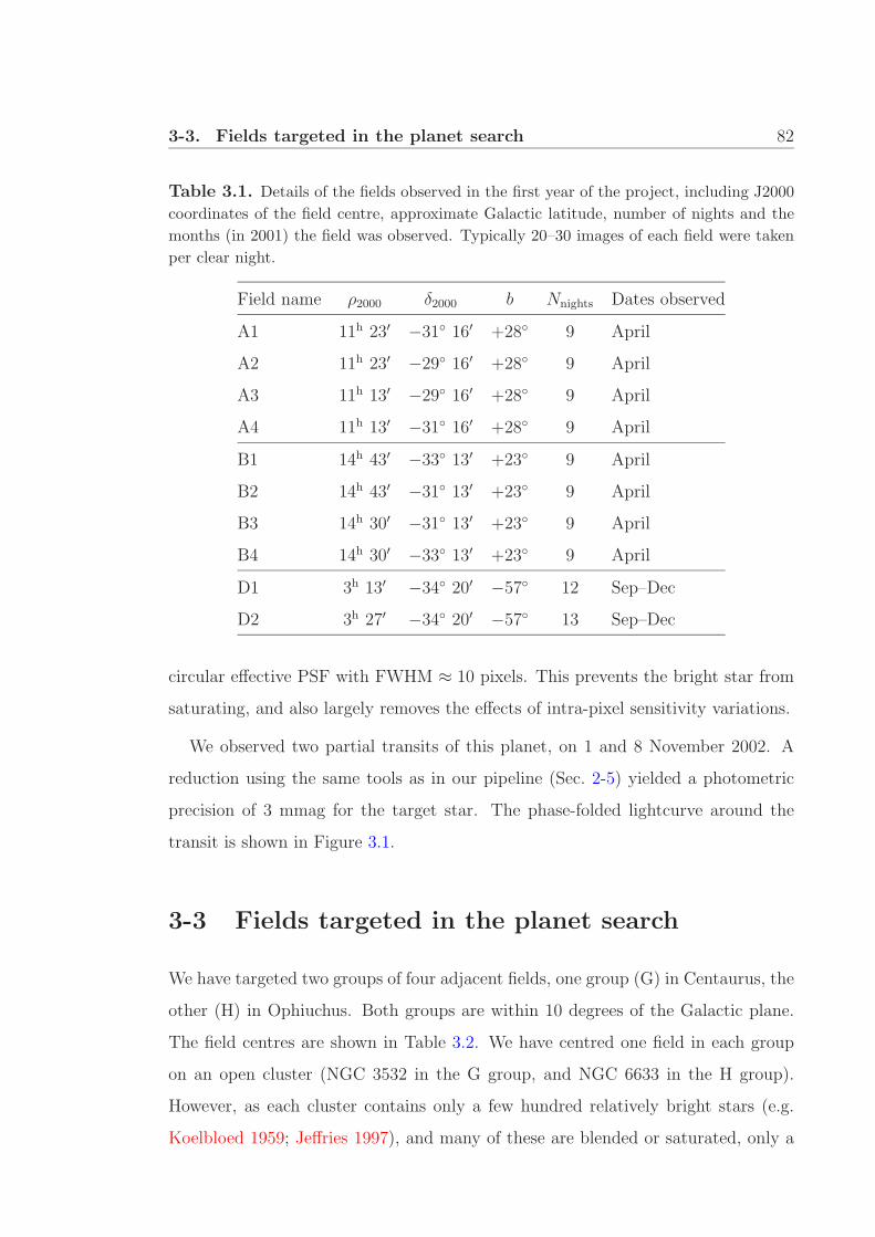
3-3. Fields targeted in the planet search 82
Table 3.1. Details of the fields observed in the first year of the project, including J2000coordinates of the field centre, approximate Galactic latitude, number of nights and themonths (in 2001) the field was observed. Typically 20–30 images of each field were takenper clear night.
Field name ρ2000 δ2000 b Nnights Dates observed
A1 11h 23′ −31 16′ +28 9 April
A2 11h 23′ −29 16′ +28 9 April
A3 11h 13′ −29 16′ +28 9 April
A4 11h 13′ −31 16′ +28 9 April
B1 14h 43′ −33 13′ +23 9 April
B2 14h 43′ −31 13′ +23 9 April
B3 14h 30′ −31 13′ +23 9 April
B4 14h 30′ −33 13′ +23 9 April
D1 3h 13′ −34 20′ −57 12 Sep–Dec
D2 3h 27′ −34 20′ −57 13 Sep–Dec
circular effective PSF with FWHM ≈ 10 pixels. This prevents the bright star from
saturating, and also largely removes the effects of intra-pixel sensitivity variations.
We observed two partial transits of this planet, on 1 and 8 November 2002. A
reduction using the same tools as in our pipeline (Sec. 2-5) yielded a photometric
precision of 3 mmag for the target star. The phase-folded lightcurve around the
transit is shown in Figure 3.1.
3-3 Fields targeted in the planet search
We have targeted two groups of four adjacent fields, one group (G) in Centaurus, the
other (H) in Ophiuchus. Both groups are within 10 degrees of the Galactic plane.
The field centres are shown in Table 3.2. We have centred one field in each group
on an open cluster (NGC 3532 in the G group, and NGC 6633 in the H group).
However, as each cluster contains only a few hundred relatively bright stars (e.g.
Koelbloed 1959; Jeffries 1997), and many of these are blended or saturated, only a

3-3. Fields targeted in the planet search 83
Figure 3.1. Transit of the planet HD 209458 b, observed by the APT. The effectsof undersampling and intra-pixel sensitivity variations were removed by defocusing thetelescope so that the PSF had a width of ∼ 10 pixels. The relative photometry wascalibrated by subtracting the (boxcar-smoothed) lightcurve of a single reference star. Thesolid line is the expected transit lightcurve based on the parameters of the system asdetermined by Brown et al. (2001). The dashed lines represent the effects of varying theplanet’s radius by ±10% in the model.
small fraction of the stars we measure in these fields are cluster members.
A third group of four fields (E), at higher galactic latitude, was also observed in
December 2002, and November–December 2003. However, because the nights are
relatively short (∼ 6.5 hours) during these summer months, and these fields were
given lower priority (because they contain fewer stars), we did not obtain sufficient
data on them for a reasonable planet detection rate. Therefore we have not analysed
the lightcurves from these fields.
3-3.1 Summary of observations in 2002–2004
The first observations using the raster-scan technique (Sec. 2-4.1) were taken in
August 2002, targeting the open cluster NGC 6633 as part of a multi-site campaign
(Martın et al. 2004) searching for variable stars. Over eight consecutive nights (7–
14 August), a total of 690 images were taken through a Johnson V filter, with
150 second exposures. In order to test the improvement due to the new technique,

3-3. Fields targeted in the planet search 84
Table 3.2. Details of fields targeted in the planet search: J2000 coordinates of thefield centre, approximate Galactic latitude, approximate number of relatively bright stars,number of nights the field was observed in 2002–2004 (ignoring nights where fewer than12 images of the field were taken), and approximate number of images obtained. Themajority of these were taken in V band (the rest were in R and I, see text for details). Insome cases a significant fraction of the images were rejected during processing.
Field name ρ2000 δ2000 b N∗(V < 14) Nnt Nim
E1 6h 04′ −30 50′ −25 1800 12 230
E2 6h 21′ −32 12′ −25 2100 12 230
E3 5h 48′ −30 50′ −25 1500 11 210
E4 6h 13′ −16 18′ −15 2400 11 210
NGC 3532 11h 07′ −58 42′ +1 7000 61 1500
G1 11h 31′ −58 42′ +3 7000 65 1700
G2 11h 31′ −56 30′ +5 7000 60 1400
G3 11h 07′ −56 30′ +4 7000 59 1400
NGC 6633 18h 28′ +6 35′ +8 5000 79 3800
H1 18h 28′ +4 30′ +7 4000 47 2000
H4 18h 41′ +4 30′ +4 3000 30 600
H5 18h 41′ +6 35′ +5 5000 30 600
on one of these nights (the 10th) the raster-scan was not used, while on the last two
nights, it was set to cover a 2 × 2 pixel area, instead of the usual 1 pixel. Later
analysis of the images revealed that the camera was slightly out of focus throughout
this run, making this data non-ideal for evaluating the new technique. Nevertheless,
the raster scan did improve the photometric precision (Fig. 3.2). In the previous
month (July 7–9), some test observations of this field with a simpler PSF-broadening
technique were also taken, yielding another ∼ 300 useful images.
In 2003 we added the three adjacent H fields, and obtained ∼ 400 images of each
(∼ 500 for NGC 6633). Roughly half of these images were taken in R. In that year
we also began observing the G group, collecting ∼ 300 images of each field in V .
In 2004 we continued to observe in V band, obtaining over 1000 images of each

3-3. Fields targeted in the planet search 85
of the G fields. We stopped observing the fields H4 and H5, in order to increase the
sampling frequency for the other two fields. On some nights we focused entirely on
NGC 6633, while on others we alternated between it and H1 (and on a few nights
we still observed all four fields). Finally, in August 2004 we observed these last two
fields in I band, obtaining about 200 images of NGC 6633 and 1100 of H1. The
exposure times were reduced to 60 seconds, as the CCD is more sensitive in this
band.
In March–August 2003 there was a problem with the camera shutter, which in-
termittently failed to open. Initially this only affected a few images each night, but
by the end of this period, as many as half the “exposures” were being taken with
the shutter closed. The shutter was repaired in mid-August 2003, and has been
working perfectly since then. Also, about 1/3 of the data on the H fields taken in
2004 (and on a few nights in previous years) were made essentially unusable due
to a mechanical problem. During the first part of most nights, the camera tilted
slightly in its mount, bringing one corner of the CCD out of the focal plane. As
the telescope orientation changed during the night, the camera settled back into its
place. Combined with the crowding in these fields, the focus changes lead to sudden
jumps in the lightcurves (more details in Sec. 3-5). These technical problems have
reduced the extent of continuous nightly monitoring of our fields, and thus have
significantly reduced the usefulness of the data for planet searching.
Due to its Northern declination, the H group of fields can be observed for a
maximum of 7 hours per night at relatively low airmass. From experience, useful
images can be taken up to an airmass of ∼ 2.2. The minimum airmass reached by
these fields is ∼ 1.3. The G fields, being much further South, can be observed for
8 hours continuously, at airmass ranging from just over 1.1 to around 1.5. Of course
these maximum times can only be reached at times of the year when the fields cross
the meridian close to midnight. In 2003 and early 2004, since we were following the
same fields for ∼ 4 months, we often observed on nights when the fields were only
reachable for 3–4 hours. Part of our revised observing strategy is to only observe
each field over the 2 months or so when it is overhead near midnight, yielding more

3-4. Photometric precision 86
Table 3.3. Details of latest fields targeted in the planet search, using our new observingstrategy. Columns are as in Table 3.2, except that the number of stars with I < 14 isgiven, as all images of these fields are in I band.
Field name ρ2000 δ2000 b N∗(I < 14) Nnt Nim
L1 4h 56′ −30 00′ −37 2000 37 2000
L2 4h 45′ −26 18′ −38 2000 37 2000
useful, longer nightly lightcurves.
3-3.2 Latest fields
Recently, we have begun selecting fields in pairs, to be observed with 60 sec exposures
in I band, giving better sampled lightcurves. We observed the first such pair (L1 &
L2) as part of a group of four potential fields in October 2004, and then intensively
in November and December 2004. Details are shown in Table 3.3. Unfortunately
the camera-tilt problem mentioned above has also affected images taken of these
fields, until mid-December, when the camera mount was fixed. More recent data no
longer shows the large magnitude jumps caused by the tilt problem, though lower
amplitude systematics do remain.
3-4 Photometric precision
The relative photometric precision achieved on a single clear night, and over several
nights of observations, is shown in Fig. 3.2. For stars in the range 9 <∼ V <∼ 11,
we routinely achieve a nightly RMS of 2 mmag. Fig. 3.3 shows similar plots for
our I-band data. The sky is brighter and more variable in I band, making it the
dominant noise source for all but the brightest stars.

3-4. Photometric precision 87
Figure 3.2. Photometric precision obtained from V -band APT data (collected in August2002) using a photometry apertures 3 pixels in radius. Top panel: One night of normalobservations, without raster scan. Middle panel: One night using 1-pixel raster scan.Bottom panel: Combined data from all 5 nights of observations using 1-pixel raster scan.The average sky flux per pixel was 1000 ADU in the first two cases, and 1200 ADU in thelast case. The telescope was (unintentionally) slightly defocused during the whole run,which is the likely cause of the better than 10 mmag photometry reached even without theraster scan. The solid line in each plot is the theoretical limit, including Poisson noise inthe star flux (dot dashed) and sky flux (dashed), as given by equation 2.1. An additionalmagnitude-independent term of 1.2 mmag (dotted line) represents scintillation, as wellas any residual errors due to flatfielding, non-linearity, and IPSV. Stars brighter thanV ≈ 9 are saturated in these 150-second exposures. Note that the magnitude zero-pointis uncertain by about 0.1 mag.

3-5. Systematic errors 88
Figure 3.3. Photometric precision from 60-second I-band images of the H1 field, ob-tained on 22 August 2004. The lines are as in Figure 3.2. Left panel: RMS noise over theentire night’s data (5 hours). Right panel: The noise if only the best 90 consecutive imagesare considered, corresponding to a 2.5 hour period when the field was at airmass below1.4. The lower airmass reduces the scintillation limit. The constant noise term in themodel (dotted line) has been reduced to 0.9 mmag. The mean sky brightness (3500 ADU)is also slightly lower than over the full night (4000 ADU).
3-5 Systematic errors
The relative photometric calibration we apply effectively removes systematic varia-
tions in apparent magnitude common to all stars, and gives close to Poisson-limited
photometric precision. However, in some of the lightcurves, systematic trends do
remain. We note that similar trends have been observed in lightcurves from other
photometric surveys, such as HATNet (Bakos et al. 2004), MACHO (Drake & Cook
2004), and OGLE (Udalski et al. 2003), though the latter authors also report that
these can be removed using a method developed by Kruszewski & Semeniuk (2003).
In our data, we have observed two types of trends, gradual changes over a night,
and more sudden changes.
3-5.1 Gradual changes
These are usually in the form of an approximately linear change in apparent mag-
nitude with time, amounting to a ∼ 10 mmag decrease or increase over the course
of a typical 6-hour night. For the worst-affected stars (usually the fainter stars, and
those near the edges of the field), the total change can be as large as 100 mmag.

3-5. Systematic errors 89
Figure 3.4. Example of the gradual systematic trends observed in many of thelightcurves. These observations were taken in I band. Each night is labelled with thevalue of JD-2450000 at UT noon, which corresponds to 0 on the time axis. The first nightis 16 August 2004.
An example is shown in Figure 3.4. In I band data on the H1 field, slightly over
half the stars have slopes of 10 mmag or more per 6 hours. On top of this trend,
some lightcurves also “curve down” at the beginning and end of the night (i.e. the
first/last few magnitudes are fainter than expected).
Other features of these trends include the following.
• On average, the slope of the trends is more positive (i.e. the star appears to get
fainter more rapidly) for faint stars, but also shows greater scatter than among
the brighter stars.
• For the fainter stars, the slope is greater in measurements made with a larger
photometry aperture.
• If a star is affected, it usually shows the same trend, with approximately the
same slope, every night. However, we have also found exceptions to this.
• Close inspection of the images did not reveal any clear tendency for the affected

3-5. Systematic errors 90
stars to have bright pixels near their aperture boundaries.
• In some data, the slope of the systematic trends appears to be correlated with
position on the CCD, though this may be a consequence of the varying density of
stars across the field. In fields at low Galactic latitude, such variations (probably
due to patchy interstellar extinction) are clearly visible in the images.
• We have found no evidence of any significant correlation between the slope of
the trends and star colour.
We believe these systematics are largely due to the inability of our sky fitting
routine to accurately follow changes in the effective background signal over small
spatial scales. This can occur in regions of the field where the density of faint, unre-
solved background stars is high (e.g. near the centre of an open cluster). Combined
with the time-dependent slope in the intrinsic sky brightness, this can lead to the
kind of trends we observe.
We have tested this by generating a set of images from a single real APT image,
adding a different sky slope to each. With perfect sky subtraction, measurements of
each star in this set should be exactly constant. While most of the lightcurves are
indeed flat, slopes do appear for some stars near the edges of the field. These are
regions where the sky subtraction fails because interpolation can only be done along
one axis. Also, there is some residual vignetting present in the corners,1 which
constitutes a small-scale variation in the effective background.
We have considered ways of improving the sky fitting algorithm in order to min-
imise these effects. One possibility (suggested by M. Ashley) is to model the “intrin-
sic sky” for a field (due to faint background stars) and subtract it from each image.
Any further sky fit should then be a simple linear function of CCD coordinates
(representing the change in the actual sky brightness).
1 The vignetting is caused by the filter casing. We suspect the reason it is not entirely removedby flatfielding is the contamination of the images by stray light (possibly moonlight) entering thetelescope from outside the field of view.

3-5. Systematic errors 91
3-5.2 Sudden changes
Small changes in the camera focus also lead to systematic errors in the photometry
on crowded fields, as they alter the contribution of light to each star’s photometry
aperture from blended or nearby stars. Since the magnitude of this change varies
depending on each star’s immediate neighbourhood, it cannot easily be corrected for.
The focus is stable over the course of a typical observing run. However, it does need
to be reset occasionally, in particular after a filter change. This can cause magnitude
offsets from night to night in the lightcurves of some stars (those which are less, or
more, affected by blending than the average reference star used for calibration).
Small magnitude offsets of this kind exist in many of the lightcurves, but are
relatively easy to remove. However, in our data on the H group of fields obtained
in 2004, we often find sudden magnitude offsets (of order 10 mmag) during a night
(Fig. 3.5). These are due to a problem with the camera mount mechanism, which
allows the CCD to tilt and move slightly out of the focal plane when the telescope
is pointing far from the zenith, towards the North-East.2
Except for a short period where the camera appears to move during the exposure
(distorting the PSF), the overall effect is that the PSF varies gradually across the
CCD, being broader by ∼ 0.3 pixel on average. Stars are measurable with reasonable
precision in most of the affected images, but because the effect depends on each star’s
position and immediate neighbourhood, these measurements cannot be calibrated to
match those from the unaffected images. Therefore we have excluded these images
from our analysis. Stronger springs have recently been installed in the camera
mount, and data obtained in the future should not be affected by this problem.
3-5.3 Removing systematic trends
The gradual systematic trends affecting our lightcurves still require further inves-
tigation. A more detailed understanding may allow us to remove them “at the
2 The camera is held in place by springs, ideally allowing only a slight movement along theoptical axis for focusing.

3-5. Systematic errors 92
Figure 3.5. Example of the systematic errors caused by the camera-tilt problem. Theseobservations were taken in V band. Each night is labelled with the value of JD-2450000at UT noon, which corresponds to 0 on the time axis. The first night is 11 April 2004.
source” by making appropriate changes to the reduction software (or even the ob-
serving strategy). An alternative approach is to attempt removing the trends by
post-reduction processing of the lightcurves.
We have made a very basic first attempt at removing the gradual systematic
trends. Since the slopes for a given star are similar each night, a single slope is
fitted and subtracted from each night of the lightcurve. After this slope correction,
night to night differences in the median magnitude of the star are also subtracted.3
In general, this simple algorithm will not preserve any long-term variations in-
trinsic to variable stars, but should preserve a transit signal in an otherwise flat
lightcurve, provided the transits affect only a small fraction of the data. In the
unlikely case that an entire night in a lightcurve is in the flat part of a transit, this
procedure would remove the signal we are looking for. However, such a signal would
not, in itself, be considered good evidence for a transit, as small night-to-night off-
3 In fact, the magnitude we want to “align” in each night is the out-of-transit magnitude, whichmay differ significantly from the median in the most important case, on a night where a transit isobserved. Therefore, instead of the median level, we subtract the 33rd percentile from each night’sdata.

3-5. Systematic errors 93
Figure 3.6. The result of applying a basic trend removal process to the lightcurve shownin Fig. 3.4.
sets occur in many lightcurves. Fig. 3.6 shows the result of applying this procedure
to the lightcurve in Fig. 3.4.
This simple trend removal algorithm has been of some use for processing
lightcurves that are to be inspected visually. However, it only removes some of
the systematics that change linearly with time. In order to make transit detection
by automated software possible, a more rigorous approach, such as the trend filtering
algorithm developed by Kovacs, Bakos & Noyes (2004) is required. Our first exper-
iments applying this algorithm to APT lightcurves are described in Section 4-1.3.

Chapter 4
Analysis & Results
The best quality data we obtained during 2002–2004 is of the NGC 6633 field
(Sec. 3-3). Therefore most of our initial detection efforts focused on this field. This
chapter describes these efforts and the resulting detections. Candidates obtained
from other fields are also mentioned.
4-1 Candidate selection
4-1.1 Visual inspection
The simplest, if somewhat time-consuming, method of detecting any kind of vari-
ability is to visually inspect the lightcurves. One advantage is that a human observer
can (in most cases) easily tell the difference between a real transit-like signal, a vari-
able star, and a spurious signal due to some systematic effect. As a consequence,
a list of variable stars (and stars affected by systematics) is also generated by this
process. The potential to detect transits is also relatively unaffected by the gradual
systematic trends described in Section 3-5.
However, there are some significant limitations of this “eyeballing” approach.
Shallow signals close to or below the noise level are difficult to pick out visually.
The periodicity of a transit signal cannot be practically exploited. Also, given that

4-1. Candidate selection 95
finding patterns is a fundamental and instinctive function of the brain, noisy but
otherwise constant lightcurves may be seen as containing signals. Perhaps most
importantly, the sensitivity of this detection method is difficult to quantify. It is
likely to vary from person to person, and depend on a number of other factors, such
as the way the lightcurves are plotted, and the time taken to view each one.
Nevertheless, we have performed such a search on the brightest 2–3000 stars in
most of the main fields we have observed to date. In the case of the NGC 6633
field, each lightcurve was eyeballed independently by at least two people, in order
to increase the probability of detecting all significant signals.
The sensitivity of this approach can be improved by optimising the way the
lightcurves are presented. Something as simple as drawing a horizontal line across
the lightcurve to indicate the mean level can help. Recently we have been pre-
processing the lightcurves to remove any nightly linear trends (Sec. 3-5.3), though
in data from less crowded fields this has not been necessary. A sample lightcurve is
shown in Fig. 4.1. Another idea (which we have not yet implemented) is to over-plot
a smoothed version of the lightcurve, assisting the identification of shallow signals.
4-1.2 Software detection
A practical and rigorous search for transit signals in the large data sets we accumu-
late is only possible using automated software. A number of detection algorithms
have been developed for this purpose (Sec. 1-6.3).
We use the algorithm (and software) of Aigrain & Irwin (2004). Lightcurves are
first searched for individual, box-shaped transit events of a given trial duration, and
the signal-to-noise ratio (S/N) of a potential transit at each of a set of trial epochs
is stored. These S/N values are then used to perform a period search. This is
repeated for a number of trial durations, and the combination of period, duration
and starting epoch resulting in the highest total S/N (over all observed transits) is
selected for each lightcurve.
A number of selection criteria are applied, based on the signal-to-noise ratios

4-1. Candidate selection 96
Figure 4.1. Example of a lightcurve plot as used in visual detection of transit-likesignals. The lightcurve shown is that of the candidate UNSW-TR-2, from the August2002 data.
for the best individual transit ((S/N)1) and all transits ((S/N)tot), as well as the
distribution of S/N values (over all trial parameters) for each lightcurve. The criteria
we have experimented with (varying the actual limits somewhat) are as follows:
1. At least two partial transits detected;
2. (S/N)tot ≥ (S/N)min, where (S/N)min needs to be at least 15 to reject the
majority of detections due to systematics;
3. (S/N)tot/(S/N)1 ≥ 1.1 to ensure that we really do have multiple transits.
To date, the effectiveness of this algorithm has been limited by the presence of
systematic trends in our lightcurves (Sec. 3-5), which lead to spurious detections in
most lightcurves. These false detections can have a high S/N (at least 10 in most
cases), and therefore may be selected as the best fit even if a true transit signal is
present. Furthermore, because the model being compared to the lightcurve assumes
a constant level outside the transits, the presence of systematics reduces the S/N
of a real signal.

4-1. Candidate selection 97
Most systematic trends are detected with periods very close to multiples of a day
(or half a day), so the problem is slightly reduced by ignoring these periods at the
initial period search stage. However in most cases the highest S/N value still results
from the systematics, folded at a different period.
Detection of a true signal in the presence of systematics may still be possible,
provided the true signal yields a high enough S/N value. This would require all
trial models meeting some minimal criteria to be “shortlisted”, not just the best one
for each lightcurve. The resulting list of models — to be visually compared to the
lightcurve — would be longer than the initial input list of stars. However, it could be
sorted in order of decreasing S/N , giving priority to the most promising candidates.
Each time a model is identified as the result of a spurious signal, all other models
with transits at similar epochs could also be rejected. Also, the visual inspection in
this case would be aided by the fact that the lightcurve can be folded at the trial
period. We have not tested this sort of “software assisted” visual inspection, but it
may offer some improvement over simple eyeballing.
The candidates selected by any method will, of course, need to be confirmed
visually. However, a fully automated algorithm, producing only a relatively small
number of candidates with a reasonable false-alarm rate, would be the most efficient
approach. To make this possible, the lightcurves will need to be pre-processed to
minimise the systematics.
4-1.3 A trend filtering algorithm
Kovacs, Bakos & Noyes (2004) have recently published details of a trend filtering
algorithm, which substantially improves the quality of lightcurves obtained by the
HATNet project (Bakos et al. 2004). Their algorithm uses a small subset of the
lightcurves as a basis set, from which a best-fit model to each remaining lightcurve
is constructed. If the basis set adequately represents the range of systematic trends
in the data, subtracting this model will remove any of these trends, leaving only the
variations intrinsic to the star.

4-1. Candidate selection 98
We have made a first attempt at implementing this algorithm. The result is a
drastic reduction of the signal-to-noise ratio of systematic trends in the lightcurves,
and far fewer spurious candidates from the detection software. Unfortunately, our
current rough implementation achieves this by not only reducing the amplitude
of the systematics, but also slightly increasing the white noise. Model transits
inserted into the lightcurves are preserved by the filter, but their S/N is also reduced.
However, Kovacs et al. (2004) have shown that the algorithm is capable of producing
significantly better results than this. In some cases, test transit signals as shallow as
5 mmag become detectable in the filtered lightcurves, while the detection probability
for 15 mmag transits approaches 100% (see their Tables 2 and 3). We believe that
with further refinement, of our implementation will achieve similar results.
4-1.4 A possible improvement to the detection algorithm
Aigrain & Irwin (2004) argue in favour of generating successive trial signals with
equal steps in trial frequency. This is to limit the change in phase of a signal near
the end of the lightcurve between consecutive trial frequencies. Most transit search
algorithms take either this approach, or use even sampling in period. In fact, for
practical reasons (see below), the version of the Aigrain & Irwin (2004) software we
use also samples the phase space with even period steps.
However, the signals we are searching for consist of short-duration events, rather
than being continuously varying. Therefore it is really the change in epoch of the
trial signals that should be limited. Consider a lightcurve containing true transits,
being searched by the algorithm. Assume that, for a given trial duration (D) and
epoch, the first transit in the lightcurve is matched exactly. With this first epoch
fixed, changing the trial period from P to P + ∆P results in a change in the epoch
of the last trial signal of ∆tlast = Nt∆P , where Nt ≈ T/P is the number of transits
in the lightcurve of total length T . In order to ensure that the last transit is also
well matched, we need to have ∆tlast < fD, where f is a small fraction (say 1/4 or

4-1. Candidate selection 99
less). That is, the inequality∆P
P<
fD
T(4.1)
should hold for all trial periods P . This can be done by simply choosing a ∆P
small enough that the condition is true at the shortest trial period. However, at the
longer periods, this will lead to a large number of superfluous trial periods. Simi-
larly, choosing a fixed frequency step (∆ν) small enough to satisfy the condition 4.1
over the whole range (with ∆ν/ν = ∆P/P ) will lead to oversampling at the high
frequencies. The optimum strategy, it seems, is to select trial periods spaced evenly
in log(P ) or log(ν). This approach will not give greater detection efficiency (if the
linear period or frequency steps are sufficiently small), but it will significantly reduce
the computation time. It could also allow a larger number of trial durations and
epochs to be tested.
As described in Section 4-1.2 above, the software of Aigrain & Irwin (2004) uses
the pre-computed single-transit detection statistics ((S/N)1) to evaluate the multi-
transit total S/N during the period search. This “trick” makes the algorithm much
more efficient, but requires the use of a constant ∆P equal to the epoch step at which
the (S/N)1 values were calculated. This last requirement ensures that, for every trial
period, all trial transits occur at epochs where (S/N)1 has already been calculated.
However, if these single-transit values are evaluated at sufficiently closely spaced
epochs (equal to or shorter than the average time between points in the lightcurve),
the (S/N)1 at any epoch could reliably be approximated. This would allow the same
trick to be used in combination with uniform logarithmic period sampling, resulting
in the most efficient use of computer resources. These considerations are perhaps
not so important for our type of transit search, as we are only searching a relatively
small period range in short lightcurves.1 However, in the case of a space mission like
NASA’s Kepler (Borucki et al. 2003), which will aim to find longer-period planets
and accumulate much larger data sets over a longer time span, these improvements
could be important.
1 As will be seen later, the two-year-long lightcurves we have obtained so far are far from ideal,and our future lightcurves will span at most 2 months.

4-2. Eliminating false positives 100
4-2 Eliminating false positives
As discussed in Section 1-6.4, the majority of transit-like signals are due to eclipsing
binary (EB) stars. Though interesting in their own right, for our planet search these
are “false-positives”, to be identified and removed from our candidate lists. Our
follow-up strategy is outlined below. At each stage we focus on the most promising
planet candidates. Depending on the available observing time we also follow up
likely binary systems.
1. Inspection of a higher-resolution image from the Digitised Sky Survey,2 to reveal
how much blending is present in the APT photometry aperture. The fraction
of the aperture flux coming from the brightest star in the aperture can also be
roughly estimated.
2. Estimation of the physical parameters of the system from the lightcurve as
described in Seager & Mallen-Ornelas (2003) (see Sec. 1-6.4). Assuming the
transit is in front of the brightest star in the APT aperture and adjusting the
transit depth accordingly gives a lower limit on the size of the transiting object.
3. Photometric monitoring of the target area at higher spatial resolution, during a
predicted transit, to identify the host of the transiting object, and measure the
true (or at least less diluted) transit depth. Alternate images are taken in V
and I, so that the colour signature of a grazing or blended eclipsing binary can
be detected.
4. Medium-resolution spectroscopic follow-up to identify the host star’s spectral
class, allowing a more precise estimate of its radius, and therefore the radius of
the planet. The presence of double spectral lines, features from different spectral
types, and in particular large radial velocity variations in phase with the transit
signal would indicate a binary or blend.
2 The Digitised Sky Survey was produced at the Space Telescope Science Institute under U.S.Government grant NAG W-2166, based on photographic data obtained using the Oschin Schmidtand UK Schmidt telescopes.

4-3. Transit candidates in the NGC 6633 field 101
5. For the best candidates, high-precision radial velocity measurements (using
echelle spectroscopy) will allow the measurement of the transiting object’s mass
and confirm or rule out its planetary nature.
Conveniently, all the above follow-up observations can be obtained at Siding
Spring Observatory. The imager on the 40-inch telescope provides seeing-limited
resolution and we have shown that better than 10-mmag photometric precision is
possible. The Double Beam Spectrograph (DBS) on the 2.3-metre telescope is ideal
for obtaining medium-resolution spectra of our candidates. The UCLES echelle
spectrograph on the 3.9 m Anglo-Australian Telescope is already being used for a
successful radial-velocity search (e.g. McCarthy et al. 2004).
4-3 Transit candidates in the NGC 6633 field
The lightcurves for the brightest ∼ 2000 stars (down to V ≈ 13) were searched
for transit-like events by visual inspection. Only the 8 nights of high-cadence data
obtained in August 2002 were used for this purpose. The more sparsely sampled
lightcurves from later years were of much poorer quality, and frequently affected by
systematic errors (Sec. 3-5). Even in the 2002 data, we found several transit-like
events which were caused by the camera-tilt problem. The 2003 and 2004 data were
only used to search for additional signals in the lightcurves of tentative candidates.
The lightcurves we eyeballed were generated using photometry apertures of radius
3 pixels. The measurements made with 2-pixel apertures were also checked for each
candidate. In some cases the absence of the signal in the smaller aperture was used
to rule out a candidate.
We identified four objects with real transits shallow enough (< 100 mmag) to be
considered as potential planet candidates. Their lightcurves are shown in Fig. 4.2.
Four additional tentative candidates, with apparent 10–40 mmag transits, were later
identified as spurious signals due to systematic errors.
Table 4.1 summarises the properties of the candidates, including an estimate

4-3. Transit candidates in the NGC 6633 field 102
Table
4.1
.Tra
nsit
cand
idat
esin
the
NG
C66
33fie
ld:
coor
dina
tes
and
para
met
ers
esti
mat
edfr
omA
PT
data
.T
cis
the
tim
eat
the
cent
reof
the
first
tran
sit
we
dete
cted
(JD
-245
0000
).C
oord
inat
esar
efr
omth
eW
CS
solu
tion
inth
eA
PT
imag
es,an
dre
pres
ent
the
cent
roid
(to
wit
hin∼
1′′ )
ofth
eob
ject
,w
hich
may
bea
blen
d.Si
mila
rly,
the
give
nV
mag
nitu
des,
wit
her
rors
of∼
0.1
mag
,ar
efo
rth
ebl
end
asm
easu
red
byth
eA
PT
.Err
ors
inth
eot
her
mea
sure
dpa
ram
eter
sar
e5×
10−
5d
for
the
peri
od,0
.01
dfo
rT
c,5
mm
agfo
rth
etr
ansi
tde
pth
(∆F
),an
d∼
0.5
hrfo
rt T
and
t F(t
hedu
rati
onof
the
com
plet
etr
ansi
t,an
dof
the
“flat
bott
om”
part
,re
spec
tive
ly).
Est
imat
esfo
rth
era
dius
ofth
est
ar(R
∗)an
dth
epl
anet
(Rp)
wer
ede
rive
dus
ing
the
equa
tion
sof
Seag
er&
Mal
len-
Orn
elas
(200
3).
IDρ
2000
δ 2000
VP
Tc
∆F
t Tt F
R∗
Rp
(day
s)(d
ays)
(mm
ag)
(hr)
(hr)
(R
)(R
Jup)
UN
SW
-TR
-118
2904
.4+
0626
5411
.02.
3807
924
96.9
330
3.4
2.0
1.4
2.9
UN
SW
-TR
-218
3051
.9+
0709
2012
.01.
0583
724
62.9
925
1.9
0.2
1.5
2.4
UN
SW
-TR
-318
3100
.7+
0708
2513
.01.
8174
924
99.0
770
2.0
0.5
0.8
2.0
UN
SW
-TR
-418
3222
.3+
0637
1312
.94.
3999
524
65.1
350
3.8
0.7
1.2
3.8

4-3. Transit candidates in the NGC 6633 field 103
Figure 4.2. Phase-folded lightcurves of the 4 transit candidates found in the NGC 6633
field. The lightcurves include all V -band data of reasonable photometric quality (nightly
rms ≤ 10 mmag and at least 10 points per night) we obtained in 2002–2004. Note that
UNSW-TR-2 is folded at its originally estimated period. Follow-up observations have
shown that this is a binary system with two nearly identical eclipses, and the true period
is twice this value.

4-3. Transit candidates in the NGC 6633 field 104
of the transiting object’s minimum radius. An inspection of Digitised Sky Survey
images (Fig. 4.3) revealed that each candidate was affected by some level of blending
in the APT photometry aperture. This has been taken into account in the radius
estimates.
A search on the Simbad online catalogue3 identified UNSW-TR-1 as a member of
the cluster (NGC 6633 141), with spectral type A2. Its radius is therefore somewhat
larger (∼ 2 R, assuming it is on the main sequence) than our estimate from the
lightcurve, making the companion radius proportionally larger also (∼ 4 RJup). The
other three candidates were not found on Simbad. For these, a rough estimate of the
spectral type can be made from their B and V magnitudes (obtained via the VizieR
service). Assuming they are main sequence stars and adjusting for the colour excess
of the cluster (E(B−V ) = 0.17, Cameron 1985), UNSW-TR-2 is F0 (R∗ ≈ 1.5 R,
in agreement with our estimate from the lightcurve), UNSW-TR-3 is F2 (1.4 R),
and UNSW-TR-4 is G2 (1 R). For the latter two candidates, these stellar radii
would yield companion radii of 3.5 RJup and 3.2 RJup respectively.
With relatively large radii, our candidates seemed unlikely to be planets. The
largest extrasolar planet known to date (HD 209458b) has a radius of 1.35 RJup
(Brown et al. 2001). However in the V band, neglecting the effects of limb darken-
ing (as we have done in our calculations) results in Rp being overestimated by up
to 50% (Seager & Mallen-Ornelas 2003, Fig. 12). Though not our primary targets,
transiting brown dwarfs and low-mass stellar objects may also yield interesting re-
sults (e.g. Sec 5-3). As Drake & Cook (2004) point out, there are currently too few
transiting planet candidates with known mass to place a firm upper limit on the radii
of extrasolar planets or brown dwarfs. For these reasons we deemed these candidates
worthy of follow-up. Our follow-up observations are described in Chapter 5.
3 The Simbad and VizieR online catalogues are maintained at CDS, Strasbourg, France, andaccessed at http://simbad.u-strasbg.fr/Simbad and http://vizier.u-strasbg.fr/viz-bin/VizieR.

4-3. Transit candidates in the NGC 6633 field 105
UNSW-TR-1 UNSW-TR-1
UNSW-TR-2 UNSW-TR-2
UNSW-TR-3 UNSW-TR-3
UNSW-TR-4 UNSW-TR-4
Figure 4.3. Transit candidates from the NGC 6633 field, as seen in the APT images (leftpanels), and in Digitised Sky Survey images (right). The white circles indicate the size ofthe photometry apertures used to measure the APT images (∼ 28′′ in radius). North istowards the top of the page, East is to the left.

4-4. Variable stars in the NGC 6633 field 106
4-4 Variable stars in the NGC 6633 field
Visual inspection of the V -band lightcurves revealed the presence of 49 well-defined
variable stars. We broadly classified 33 of them as short-period pulsators (including
several likely δ Scuti stars), 5 as RR Lyrae, and two as long-period, semi-regular
variables. The remaining 9 were eclipsing binaries. Three objects on our list were
previously known variable stars. The full list is published in Hidas et al. (2005).4
4-5 Transit candidates in other fields
The lightcurves we obtained from the remaining 7 fields in the G and H groups
(Sec. 3-3) are generally of lower quality than those from the NGC 6633 field. This
is mainly because of the infrequent sampling and the technical problems we expe-
rienced. However, we did eyeball the lightcurves for the brightest ∼ 2000 stars in
the G1, G2, H4 and H5 fields. For the H1 field, we compiled a more extensive list
of lightcurves from the high-cadence I-band data obtained in August 2004 (almost
7000 lightcurves, down to I = 14). However, as this field will not be observable
again until mid-2005, we have given other fields higher priority, and to date have
only inspected about half of the H1 lightcurves.
In each of these fields the tentative transit candidate list typically included 10–
20 objects. On closer inspection and inter-comparison, many of these were seen to
have similar signals at similar times, a clear sign of systematic errors. This was
particularly common in the H fields, due to the camera-tilt problem (Sec. 3-5). A
number of other candidates were rejected because their lightcurves contained only
single transits, or secondary eclipses were clearly present.
Details of the remaining three candidates are shown in Table 4.2. The companion
radius estimates indicate that these are most likely binary stars. A search on the
Simbad online catalogue revealed that UNSW-TR-6 (HD 98623) and UNSW-TR-7
(GSC 00441-01364) are both known multiple stars, of spectral types A1 and B8
4 The list was compiled by J. Christiansen and the variables were classified by A. Derekas.

4-5. Transit candidates in other fields 107
respectively. The catalogued spectral types are consistent with the R∗ estimates in
the table, and confirm that the companions are too large to be of planetary origin.
UNSW-TR-5 was not found on Simbad. From the optical colours obtained from
VizieR, arbitrarily assuming a colour excess of E(B−V ) = 0.1, the star has spectral
type F8, and therefore a radius ∼ 1.2 R∗. This is a considerably smaller estimate
than what was obtained from the lightcurve, yielding a companion radius of 2.4 RJup.
This candidate was added to our list of targets to be followed up during our June
2004 observing run (Chapter 5).
Numerous variable stars and eclipsing binaries with deeper eclipses are also
present in these data, but we have not had time to perform a rigorous search for
these.

4-5. Transit candidates in other fields 108
Table
4.2
.C
oord
inat
esan
dpa
ram
eter
ses
tim
ated
from
the
AP
Tlig
htcu
rves
for
the
cand
idat
esfo
und
infie
lds
G1,
G2,
and
H1
(res
pec-
tive
ly).
Tra
nsit
sof
UN
SW-T
R-7
wer
efo
und
inI-b
and
data
,th
us∆
Fin
this
case
refe
rsto
the
tran
sit
dept
hin
that
band
.It
sm
edia
nm
agni
tude
inI
is8.
9.E
rror
sar
eas
inTab
le4.
1,ex
cept
that
,be
caus
eth
ese
light
curv
essp
ana
shor
ter
peri
odof
tim
e(o
nly
aw
eek
for
TR
-7),
the
unce
rtai
ntie
sin
the
peri
ods
are
larg
er.
The
yar
e0.
0002
dfo
rT
R-5
,0.
001
dfo
rT
R-6
,an
d0.
005
dfo
rT
R-7
.
IDρ
2000
δ 2000
VP
Tc
∆F
t Tt F
R∗
Rp
(day
s)(d
ays)
(mm
ag)
(hr)
(hr)
(R
)(R
Jup)
UN
SW
-TR
-511
2750
.8−
5854
5911
.73.
9222
2735
.05
454.
10.
72.
14.
2
UN
SW
-TR
-611
2012
.3−
5625
169.
34.
979
2754
.91
403.
80.
51.
83.
3
UN
SW
-TR
-718
2903
.6+
408
038.
73.
042
3237
.935
4.5
0.7
3.0
5.3

4-5. Transit candidates in other fields 109
Figure 4.4. Phase-folded lightcurves of the transit candidates found in the field G1,
G2 and H1. The lightcurves of UNSW-TR-5 and 6 are from V -band data obtained in
2003 and 2004, while that of TR-7 is from I-band observations in August 2004. TR-5
is folded at its originally estimated period. Follow-up observations have shown that the
orbital period of this binary system is twice this value. The lightcurve of TR-6 contains
a secondary eclipse at phase ∼ 0.7. The fact that it does not occur at phase 0.5 suggests
that the orbit is eccentric. TR-7 shows out-of-eclipse ellipsoidal variations pointing to a
stellar-mass companion (Sec. 1-6.4).

Chapter 5
Follow-up Observations
Having found our first candidates, we requested time on two of the larger telescopes
at Siding Spring Observatory (SSO) so that we could identify the source of these
signals. We were granted a total of 11 nights on the 2.3-metre telescope, and 14
nights on the 40-inch. These observations also allowed us to gain valuable experience
and demonstrate our ability to follow up candidates efficiently.
Along with the objects listed in Table 4.1, our target list included some more
tentative candidates (2 from the NGC 6633 field, 5 from G1 and 1 from G2), some
of which were later discovered to be due to systematic errors.
5-1 Photometry at high spatial resolution
We obtained high spatial resolution images using the 40-inch telescope.1 The
imager uses a Tek CCD with 2k × 2k pixels to image a 20 arcmin square field (at
0.′′6 per pixel). The full CCD takes 5 minutes to read out. To obtain a reasonable
sampling frequency, we only read out one quarter of the chip, corresponding to a
10 arcmin square field.
We aimed to monitor each candidate continuously during a predicted transit,
1 The 40-inch data were obtained by myself, C. Nutto, A. Phillips, and A. Derekas, and reducedmostly by C. Nutto.

5-1. Photometry at high spatial resolution 111
alternately taking 2–3 images in each of the V and I bands. The exposure time
was frequently adjusted to maintain a high flux from our target stars in each image,
without saturating them. This was necessary because the seeing was often quite
variable. The exposure times were generally in the range 20–150 seconds.
Our observations were scheduled for the nights of 9–14 and 20–27 of June, 2004.
We lost a considerable amount of observing time due to a run of bad weather and
some technical problems with the instrument and control software. We observed
only one transit, of the candidate UNSW-TR-2, on the night of 14 June.
The data were reduced using standard tools in IRAF. Measurements were made
using the phot aperture photometry task in the noao.digiphot.apphot package,
with an aperture radius of 6 pixels. The relative photometric calibration was done us-
ing a slightly modified version of the program used in the APT pipeline (Sec. 2-5.7).
Fitting the magnitude residuals as a function of CCD position was not necessary in
this case, only a global zero-point correction was applied to each image.
In the case of UNSW-TR-2, these measurements revealed that source of the
transit signal is the second brightest star in the APT aperture (∼ 0.8 mag fainter
than the brightest one, and ∼ 10′′ from it). The star, its surroundings, and the
relative position of the APT photometry aperture are shown in Figure 5.1. The
photometry we obtained during the eclipse had a scatter of 4 mmag (RMS) in V
and 3 mmag in I on top of the eclipse signal. The undiluted lightcurve (Fig. 5.5)
shows a V-shaped eclipse with a depth of 0.14 mag, suggesting that the signal is
from a grazing eclipsing binary system. The similarity of the eclipse shape in the two
colour bands shows that the components of the system are of similar temperature.

5-2. Medium-resolution spectroscopy 112
UNSW-TR-2 UNSW-TR-2
Figure 5.1. Close-up of the candidate UNSW-TR-2, as seen in images taken with the40-inch telescope in V band (left) and I band (right). The white circles represent theAPT photometry aperture (∼ 28′′ in radius). The star which was identified as the sourceof the transit signal is indicated with a cross. North is at the top, East is to the left.
5-2 Medium-resolution spectroscopy
5-2.1 Spectra obtained
We obtained spectra using the Double-Beam Spectrograph (DBS) on the 2.3 m
telescope, also at SSO.2 Our time allocation consisted of the nights of 4–11 and 25–
27 June (2004), preceding and overlapping with the imaging run. Ideally, we would
obtain follow-up photometry first, giving us a chance to identify (at high spatial
resolution) the exact source of the transit signal, making subsequent spectroscopic
observations more efficient. This is the arrangement we will request in our future
follow-up runs.3 In the present case, we chose to obtain multi-phase spectroscopy
of only the brightest, and therefore “least diluted” star in the APT photometry
aperture of each candidate. Given a fixed transit depth in the APT lightcurve, this
is the potential host star that yields the smallest companion radius, i.e. the one that
2 In obtaining the spectra, I was helped by C. Nutto, H. Toyozumi, and J. Christiansen.A. Derekas reduced and calibrated the spectra, measured radial velocities, and fitted circular-orbitmodels to the velocity curves where possible.
3 Indeed our allocation, on the same two telescopes, in February 2005 is arranged in this way.
5-2. Medium-resolution spectroscopy 113
is most likely to be a planet. We also took single spectra of the fainter neighbouring
stars, so that at least their spectral types could be identified.
We used the highest resolution grating in both arms. The approximate spectral
ranges covered were 5700–6700 A in the red arm and 3900–4400 A in the blue, with
resolutions of 1.1 A (45 km s−1) and 0.5 A (40 km s−1) respectively. In each arm the
spectrum was imaged at a scale of ∼ 2 pixels per resolution element. The slit was
kept vertical on the sky during all observations. Exposure times varied from 600
to 900 seconds, depending on target brightness and seeing conditions. The typical
signal-to-noise ratio reached was ∼ 50 per pixel.
All the processes of image reduction, extraction of spectra and wavelength-
calibration were performed with standard tools in IRAF. The continuum in each
spectrum was normalised to unity. We were unable to wavelength-calibrate the
data obtained in the blue arm (we could not identify the lines in the arc spectra).
However, sufficiently precise radial velocity measurements were possible from the
red spectra alone.
5-2.2 Spectral types
Before our own run on the 2.3-metre telescope, we obtained a single set of low-
resolution “quick-look” spectra of the candidates in the NGC 6633 field.4 Only the
blue arm of the DBS was used, covering the range 3420–5350 A with a resolution of
2.2 A. These data were reduced in the same manner as our medium-resolution spec-
tra, but were also flux-calibrated (using a spectrum of the standard star EGGR 131,
obtained on the same night). The results are shown in Figure 5.2.
Visually comparing these low-resolution spectra to templates from the UVILIB
spectral library (Pickles 1998) yielded a spectral type estimate for each candidate.
This is by no means a rigorous stellar characterisation. However, as our main goal
here is simply to identify obvious stellar companions, even a low-precision (∼ 10%)
4 We are grateful to Anna Frebel for taking these spectra in her own observing time. Thespectra were taken on the night of 30 March 2004.

5-2. Medium-resolution spectroscopy 114
estimate of the primary’s mass is sufficient. The spectral types and masses we thus
obtained are shown in Table 5.1.
5-2.3 Radial velocities
We measured radial velocities by cross-correlation with a spectrum of the RV stan-
dard star β Vir (obtained with the same instrument). We only used the region
around the Hα absorption line (6450–6640 A) for this.
With periods as short as those of our candidates, the orbits are likely to have been
circularised by tidal dissipation (Sec. 1-4.6). Therefore we fitted simple sine-wave
models to the phased radial-velocity curves (Fig. 5.3). As the period and orbital
phase was already known from the APT lightcurves, the only free parameters in the
model were the overall velocity of the system (vs, assumed to be constant over the
duration of our observations), and the velocity amplitude of the star being measured
(K). The function fitted was vs + K sin(2πφ), where φ is the phase. The results of
the fits are listed in Table 5.1.
For three of the candidates (UNSW-TR-1, 3 and 4), the star we measured shows
large RV variations in phase with the transit signal. These are single-lined binary
systems. Estimating the mass of the primary (M1) from its spectral type, the mass
of the companion (M2) is given by numerically solving the equation (derived from
Kepler’s law)
M32
(M1 + M2)2=
(K
KE
)3P
P0
(5.1)
where the masses are in solar units, KE = 29.87 km s−1 (the Earth’s orbital velocity),
P is the period of the binary and P0 = 1 year. As shown in Table 5.1, the companions
of these three candidates, with masses of 0.2–0.4 M are most likely M dwarfs. This
is also consistent with the companion radii estimated from the APT lightcurves
(Table 4.1).
UNSW-TR-5 is a double-lined binary, with two sets of spectral lines of very similar
strength. Thus the cross-correlation yields two radial velocities at each epoch. The
average of these measurements is essentially the overall system velocity (vs), since

5-2. Medium-resolution spectroscopy 115
Figure 5.2. The “quick-look” spectra obtained for the purpose of spectral type identifi-cation (the bottom spectrum in each panel). The top spectra (vertically offset for clarity)are the closest matching templates from the UVILIB library (Pickles 1998). The observedspectra were smoothed to match the resolution of the templates (∼ 10 A). In the case ofUNSW-TR-2, the low-resolution spectrum we obtained was of the brightest star in theAPT photometry aperture. The spectrum plotted here is that of the source of the transitsignals, from our medium-resolution observations. UNSW-TR-1 appears to have suffered asignificant amount of reddening (from the spectrum, a rough estimate of the colour excessis E(B −V ) ≈ 0.5). This suggests some localised dust extinction is present along this lineof sight. If this is indeed an A2V star in the NGC 6633 cluster, at distance of ∼ 300 pc(Cameron 1985), the total extinction in V -band is ∼ 2.5 mag.

5-3. A K7V eclipsing binary system 116
Table 5.1. Parameters obtained from follow-up spectroscopy. The error on the primarymass (M1) was assumed to be 10%. In two cases (TR-2 and TR-5) the RV curve revealedthat the orbital period is double the photometric period determined from the APT data.The velocity amplitude of TR-2 was estimated from the separation of double lines in thesingle spectrum we obtained. In estimating the masses, we assumed the two stars haveequal mass. The orbit of TR-4 appears to be eccentric, but we have insufficient data fora rigorous Keplerian fit. Assuming a circular orbit gives the result quoted here.
Star ID Sp Type M1 K P M2
(M) (km s−1) (days) (M)
UNSW-TR-1 A2V 2.5 27 ± 3 2.38079 0.34 ± 0.05
UNSW-TR-2 K7V = M2 87 ± 3 2.11674 0.58 ± 0.05
UNSW-TR-3 F7V 1.2 53 ± 10 1.81749 0.4 ± 0.1
UNSW-TR-4 F5V 1.3 ∼ 20 4.39995 ∼ 0.2
UNSW-TR-5 (1) 70 ± 4 7.8442 1.0 ± 0.1
UNSW-TR-5 (2) 66 ± 4 1.0 ± 0.1
the components are likely to be of nearly equal mass (this can also seen in the
symmetry of the RV curves). Fixing vs at this value leaves only the two amplitudes
(K1 and K2) as free parameters, which were fitted independently.5 Plotting the
phased RV curves also showed that the true period is double the photometric period.
The total mass of the system is given by Kepler’s law, in the form
M1 + M2 =
(K1 + K2
KE
)3P
P0
(5.2)
which, for UNSW-TR-5 yields M1 + M2 = 2.0 ± 0.2 M. As the two velocity
amplitudes are equal to within the errors, this system consists of two solar-mass
stars.
5-3 A K7V eclipsing binary system
For the candidate UNSW-TR-2, the radial velocity of the bright star dominating
the light in the aperture showed no coherent variations when folded at the period
5 Fitting the two RV curves without fixing vs does not significantly change the best-fit ampli-tudes.
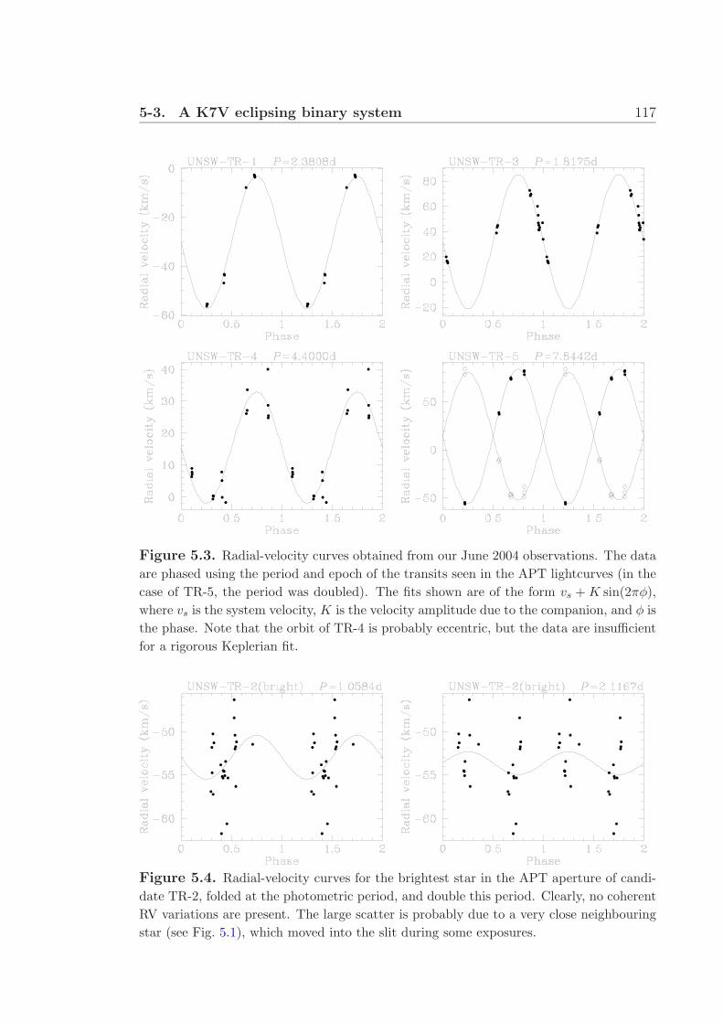
5-3. A K7V eclipsing binary system 117
Figure 5.3. Radial-velocity curves obtained from our June 2004 observations. The dataare phased using the period and epoch of the transits seen in the APT lightcurves (in thecase of TR-5, the period was doubled). The fits shown are of the form vs + K sin(2πφ),where vs is the system velocity, K is the velocity amplitude due to the companion, and φ isthe phase. Note that the orbit of TR-4 is probably eccentric, but the data are insufficientfor a rigorous Keplerian fit.
Figure 5.4. Radial-velocity curves for the brightest star in the APT aperture of candi-date TR-2, folded at the photometric period, and double this period. Clearly, no coherentRV variations are present. The large scatter is probably due to a very close neighbouringstar (see Fig. 5.1), which moved into the slit during some exposures.

5-3. A K7V eclipsing binary system 118
Figure 5.5. The undiluted eclipse signal from transit candidate UNSW-TR-2, observedat high spatial resolution with the 40-inch telescope at SSO. We observed a single transit,alternating between V band (triangles) and I band (squares). The matching shape of theeclipse in the two colours confirms that the two stars are of nearly equal temperature. Thesolid line is the model lightcurve for an eclipsing system consisting of 2 K7V stars (withmasses 0.58 M and radii 0.64 M) in an orbit with period 2.11674 days and inclinationof 83.4. The dashed lines show the result of varying the radius of the stars by ±5%(keeping other parameters constant).
measured from the transits, or at double that period (Fig. 5.4). We only obtained
one DBS spectrum of this star’s close neighbour, which was revealed in the 40-inch
images to be the source of the transit signal. This spectrum is well matched by a
K7V template, with two important exceptions:
1. there is a strong Hα emission peak; and
2. the absorption lines and the emission line all have two components of approxi-
mately equal strength.

5-3. A K7V eclipsing binary system 119
Measuring the separation of several pairs of lines,6 and adjusting for the orbital
phase at the time the spectrum was taken (sin(2πφ) = 0.973) gives a maximum
velocity separation between the components of 175 ± 6 km s−1.
We were able to obtain two more spectra of this star at lower resolution.7 Al-
though the double line structure is not completely resolved in these spectra, they do
confirm that the separation between the lines varies with orbital phase. The three
spectra are compared in Figure 5.6.
We have not performed a rigorous fit to the lightcurves. However, a model con-
sisting of two identical K7V stars, each of mass 0.58 ± 0.05 M and radius 0.64 ±
0.01 R, appears to fit all the observations. The period is 2.11674 ± 0.00002 days
(twice the original estimate), giving an orbital radius of ∼ 0.03 AU. The orbital
inclination is 83.4 ± 0.1 degrees.8
This system may be a valuable addition to the small number of known double-
lined eclipsing binary systems with late-type components, for which the phys-
ical parameters can be measured with precision (e.g. Torres & Ribas 2002;
Maceroni & Montalban 2004; C. Maceroni, private communication). Such mea-
surements provide important constraints for models of low-mass stars.
6 The separations were measured by fitting Gaussian profiles to each component using the“splot” task in IRAF.
7 The additional spectra were obtained for us by Chris Blake (while he was observing for anunrelated project) on the nights of 22 and 23 August 2004. The spectral coverage, using botharms, was 3620–7360 A, with a resolution of 2.2 A.
8 The fitted stellar radius and inclination are strongly correlated.

5-3. A K7V eclipsing binary system 120
Figure 5.6. Close-up of the region near the Hα line in the spectra of UNSW-TR-2.The top spectrum is the one we obtained on 8 June 2004, with a resolution of 1.1 A. Thebottom two were taken on 22 and 23 August 2004, with 2.2 A resolution. The numbersabove each spectrum indicate the value of sin(2πφ) at the time of the observation (whereφ is the orbital phase). Note the change in the width of the blended Hα line in the lowerresolution spectra as the separation between the components decreases. Due to a problemwith the wavelength calibration, the lower-resolution spectra had to be shifted (by +5 and−2 Angstroms, respectively) to align them with the high-resolution spectrum.

Chapter 6
Search Sensitivity and Detection
Rate
Beyond the detection and characterisation of individual planets, an important goal
of a planet search is to deduce statistical properties of the extrasolar planets from
its detections (or lack thereof). Naturally, maximising the number of detections is
also a priority. Therefore we need to have an understanding of the sensitivity of
our search, and its dependence on properties of the planets, their host stars, and on
observational parameters.
Due to the limited knowledge we currently have about the properties of extra-
solar planets and their host stars, and the simplifying assumptions we make, any
detection rate we calculate will only be an order-of-magnitude estimate. However,
if we model our observations in sufficient detail, the relative efficiency of various
observing strategies can be evaluated.
6-1 A rough estimate
The number of detectable planets in our search can be approximated as
Ndet = Ndwarf × Ppl × Ptr × Pobs

6-1. A rough estimate 122
where Ndwarf is the number of dwarf stars in our fields, for which a hot Jupiter
would cause at least a 10 mmag transit, Ppl is the fraction of stars that actually
host such a planet, Ptr is the geometric probability that the planet does transit
(i.e. that it crosses our line of sight to the star), and Pobs is the probability that
we observe multiple transits, with some minimum combined signal-to-noise ratio
((S/N)min ≈ 10).
A typical transiting hot Jupiter, with radius 1.2 RJup (see Fig. 1.2), will cause
at least a 10-mmag transit in front of any star with radius R∗ ≤ 1.2 R, i.e. of
spectral type ∼ F8 or later. For a sample limited to V <∼ 13, at least 50% of stars
are of type GKM (Cox 2000).1 Thus we have Ndwarf ≈ 0.5 × N∗, where N∗ is the
total number of stars monitored with at least 10-mmag precision (i.e. with V <∼ 13).
For the NGC 6633 field, N∗ ≈ 2000.
The frequency of hot Jupiters is Ppl ≈ 0.01 (e.g. Gaudi, Seager & Mallen-Ornelas
2005), and their transit probability is Ptr ≈ R∗/a ∼ 0.1 (a is the orbital radius).
Therefore, observing a rich Galactic field like NGC 6633, we have Ndet ≈ Pobs. For
our complete NGC 6633 lightcurves, Pobs ≈ 0.4 (minimum one complete and one
partial transit, 1 < P < 9 days, see Fig. 6.1), giving an estimate of 0.4 planets for
this dataset, or ∼ 0.2 planets per year.
In this simple estimate, we have made some gross simplifications, including (1)
neglecting the dependence of Ppl, Ptr and Pobs on the orbital period, and other prop-
erties of the star and planet; (2) neglecting the 3-dimensional distribution of stars
in the Galactic disk; (3) neglecting interstellar extinction; (4) neglecting the effect
of blends in a crowded field; (5) ignoring the possible effects of stellar companions
on detection probability (only ∼ 1/3 of late-type dwarfs are single stars, according
to Duquennoy & Mayor 1991). Therefore this is a very rough estimate indeed, but
will provide a useful comparison to the results of our more detailed analysis.
We note that Horne (2003) estimates a detection rate of 3 planets per month for
1 In the HD catalogue, 50% of stars with V ≤ 8.5 are of type GKM. A deeper sample willinclude a greater fraction of these faint, late-type stars. This is because fewer early-type stars areadded to the sample as the magnitude limit increases due to interstellar extinction and the scaleheight of the galactic disk.

6-1. A rough estimate 123
Figure 6.1. The probability of observing at least one (solid line) or two (dotted line) com-plete transits of a transiting planet in the lightcurves we have obtained for the NGC 6633field. A minimum of 100 in-transit data points are required for a detection (so that 10-mmag precision yields a total signal-to-noise ratio of at least 10 for a typical transitinghot Jupiter). A typical transit duration of 0.1 day is assumed. The one-transit proba-bility also includes the requirement of at least one additional partial transit, so that theperiod can be estimated. The mean probability over this period range (1–9 days, sampledlogarithmically) is 0.4 for one transit, and 0.3 for two transits.
our project, using simple scaling laws. However, by his calculations, all the transit
surveys combined should be detecting 191 planets each month, which is clearly an
overestimate. The main goal of these calculations was perhaps not an estimate of
the absolute detection rate, but rather a comparison of the various projects. If we
assume the six planets found by the transit method to date were detected from a
single year of observations by all the projects, and scale Horne’s estimate to match
this rate, then his estimate for our search becomes 0.09 planets per year.
For a transit search with parameters comparable to ours (though a shorter ob-

6-2. Monte Carlo simulation 124
serving run), Brown (2003) estimates a rate of ∼ 0.7 detected planet per 104 stars
monitored (to a magnitude limit of R = 12). Our estimate above translates to
∼ 2 planets per 104 stars. Brown’s analysis includes a number of effects, such as
that of the planet period and radius distributions, which reduce the detection rate
compared to our simple estimate.
6-2 Monte Carlo simulation
In order to obtain a more accurate estimate, we have modelled our observations
using a Monte Carlo simulation. This allows us to use a realistic photometric noise
model, and to take various observational effects into account (in particular blending,
and the set of epochs at which the lightcurves are sampled).
We begin by simulating a population of stars in a 1 square degree field of view.
We use the luminosity function for the Solar neighbourhood, Φ0(MV ) (as tabulated
in Cox 2000, for MV = −7,−6, ...18), allowing for an exponential drop-off with
height above the Galactic plane (with scale heights, H(MV ), from Allen 1973). The
number of stars of absolute magnitude MV per cubic parsec, at a distance d and
Galactic latitude b, is thus
Φ(MV , d, b) = Φ0(MV )e−d| sin b|/H(MV )
We divide the volume sampled by a 1 square degree field into a series of shells of
thickness 20 pc. We fill each shell with the appropriate number of stars in each MV
bin. To calculate the apparent (V ) magnitude of each star, we assume an extinction
of 1.9 magnitudes per kiloparsec in the Galactic plane, dropping off exponentially
with distance from the plane, with a scale height of 140 pc (Allen 1973). Only stars
with 5 < V < 19 are included in the model, as stars brighter than this can be
avoided during field selection, while fainter stars are not resolved in APT images
and effectively become part of the background.
Depending on MV , an appropriate fraction of stars (tabulated in Cox 2000) are

6-2. Monte Carlo simulation 125
simulated as binary systems. For simplicity, a luminosity ratio is randomly selected
from a uniform distribution in the range (0, 1).2 The absolute magnitude of the
primary is adjusted for this (keeping the total luminosity of the system equal to the
original MV ), and the secondary is ignored.
Apart from binary companions, a 3-pixel radius photometry aperture centred
on a star in an APT image typically includes light from several other stars. We
randomly assign pixel coordinates to the simulated stars, within a section of the
APT CCD corresponding to one square degree. For each star, we then calculate
what fraction of the total starlight in the aperture comes from that star (fap).3
This factor is included when calculating the observed transit depth due to a planet.
Stars for which this fraction is less than 5% are excluded from further analysis, as
any planetary transit signal from these stars would be diluted below our detection
limit.
Around each remaining star, we place a planet with a radius of 1.2 RJup. We
randomly select a period in the range 1–9 days, using the distribution described by
Gaudi et al. (2005): uniform in log P in each of two bins, 1–3 d (“very hot Jupiters”,
VHJ) and 3–9 d (“hot Jupiters”, HJ), with the frequency of VHJ relative to HJ being
15%.
Tables in Lang (1992) give the mass (M∗) and radius (R∗) of the star based on
its absolute magnitude, assuming it is on the Main Sequence. For the planet, we
assume a circular orbit, with radius a = (1 AU)(M∗/M)1/3(P/(1 yr))2/3. We then
randomly select an orbital inclination (i) leading to a transit (i.e. select cos i from a
uniform distribution in the range 0–Ptr, where Ptr ≈ R∗/a is the probability of such
an inclination for a randomly oriented orbit).
Neglecting limb-darkening, grazing transits, and ingress/egress times, we approx-
2 The observed distribution of binary mass ratios peaks near q = 0.3 and drops off considerablyat higher values (Duquennoy & Mayor 1991). Therefore on average, our simplification overesti-mates the dilution of the primary’s light by the companion, leading to a slightly lower estimate ofthe probability of detecting a planet around the primary.
3 To simplify and speed up this calculation, any star falling inside a square aperture (equal inarea to the circular apertures we actually use) is assumed to contribute 100% of its light to theaperture sum, while stars outside it contribute no flux.

6-2. Monte Carlo simulation 126
imate the signal as a rectangular transit of depth ∆F = (Rp/R∗)2, and duration
∆t =P
πa
√(R∗ + Rp)2 − (a cos i)2
We assume that we will reliably detect transits with ∆F > ∆Fmin = 10 mmag.
Provided multiple transits are observed, including at least one complete transit,
and a minimum total signal-to-noise ratio is reached ((S/N)min = 10), shallower
signals are theoretically detectable. In practice this is difficult due to systematic
trends in many of the lightcurves with amplitudes of ∼ 10 mmag (Sec. 3-5). In
fact, some of our lightcurves contain systematics with larger amplitudes, making
even the detection of 10 mmag transits unlikely. If the above additional conditions
are satisfied, 20 mmag transits are generally detectable by visual inspection, and in
most cases by the software as well.
Initial experiments with the trend filtering algorithm of Kovacs, Bakos & Noyes
(2004) are encouraging (Sec. 4-1.3), and a full implementation of the algorithm will
reduce the transit depth threshold imposed by systematics to at least 10 mmag.
We have not yet fully characterised the sensitivity of our detection software because
our filtering code still requires some fine-tuning. However, preliminary tests have
shown that in the absence of systematics, 10 mmag transits are detected in a high
percentage of cases.
We estimate the photometric precision per measurement using a noise model
which includes Poisson noise due to star and sky flux (Equation 2.1), and a limit-
ing precision of 1.5 mmag (due to scintillation, and residual errors from flatfielding,
CCD non-linearity, and intra-pixel variations). The model is comparable to the solid
curves in Fig. 3.2, but with parameters set to match the actual noise in our mea-
surements. In particular, we use the actual photometry aperture radius (3 pixels) to
calculate the sky noise, rather than the ideal, PSF-fitting case used for comparison
in the figure. The other parameter values we used (see Sec. 2-2.1) are 22.5 mag for
the magnitude zero-point, 1000 ADU/pixel for the sky flux, and 8.5 e−/ADU for
the gain.
Combined with ∆F , the calculated noise level tells us the number of in-transit

6-3. Validating the simulation 127
Figure 6.2. Left: a section of a real APT image of the NGC 6633 field (away from thecluster centre). The section shown is ∼ 40 arcmin wide. Right: a simulated image basedon the distribution of stars generated by the Monte Carlo simulation for the same Galacticlatitude (∼ 8).
measurements (Nmin) that need to be made in order to achieve a total signal-to-
noise ratio of (S/N)min = 10, which we deem sufficient for a detection. Given a
simulated planet and a set of observation epochs, we can calculate the probability
(Pobs) that a minimum of 2 complete transits will be observed,4 including at least
Nmin in-transit points. We do this by testing 1000 transit epochs, evenly distributed
over one period.
To estimate the total planet catch for a given set of observing parameters (Galac-
tic latitude and observation epochs), we add up the values of Ptr × Pobs for each
simulated planet and scale the result to the appropriate field size. We also multiply
by the fraction of stars that do host such short-period planets, which is ∼ 1% (e.g.
Gaudi et al. 2005).

6-3. Validating the simulation 128
6-3 Validating the simulation
In order to ensure that this rather complicated simulation yields reasonable results,
we performed a number of tests. Firstly, we generated a set of fake APT images
using the distribution of stars from the simulation (for b ≈ 8). The simulated
images appear very similar to a real image at the same Galactic latitude (with the
exception of some patches of increased extinction in the real image, see Fig. 6.2).
Processing these fake images through the photometry pipeline, we also confirmed
that the star counts as a function of limiting magnitude closely match those obtained
from a real image.
We then modified the simulation to reproduce the simplifying assumptions made
by Horne (2003). The result was within a factor of 2 of Horne’s estimate for our
project. Finally, we confirmed that the result scales with planet, star, and observa-
tional parameters (Rp, a, MV , R∗, d, sky brightness, survey duration and (S/N)min)
as predicted by Horne’s equations 1 and 3.
6-4 Results for the NGC 6633 field
We have simulated observations at the Galactic latitude of the NGC 6633 field
(b = 8), using the epochs of the best images we have obtained for this field in
2002–2004 (2486 images, from 61 nights over 3 seasons). We made no attempt to
simulate the cluster itself. Its effect on the planet catch is likely to be negative,
though small (the cluster adds a few bright stars to the field, but also increases
the crowding). The expected planet catch for a single 6 square degree APT field is
∼ 0.1 planets (minimum two complete transits observed). If we accept one complete
and one partial observed transit as a detection, the estimate becomes ∼ 0.2 planets,
in reasonable agreement with the rough estimate derived above.
As expected, we are most sensitive to planets with the shortest periods (Fig. 6.3,
4 In fact, we accept a transit as completely observed if the time between the first and lastin-transit points is over 90% of the transit duration.

6-4. Results for the NGC 6633 field 129
top panel). However, since we have simulated planets with periods longer than 3 d to
be almost 10 times more frequent than those with P < 3 d, the period distribution
of detected planets also has a peak at 3–5 d.
We are most likely to detect planets orbiting stars with MV ≈ 4 (Fig. 6.3, middle
panel), as also predicted by Pepper, Gould & Depoy (2003). These are the brightest
stars that are small enough for our simulated 1.2 RJup planet to cause a 10 mmag
transit. Compared to smaller stars, they have greater geometric transit probability
and, on average, longer transit times. More significantly, it is their greater number in
our magnitude-limited sample that makes them the most common host of detected
planets.
The most numerous of the the potentially detectable planets are those with the
shallowest transits. As a result, the total planet catch depends strongly on the
minimum detectable transit depth, ∆Fmin (see cases A–C in Table. 6.1 and discussion
in Sec. 6-5.1 below). For our visual inspection of the NGC 6633 lightcurves, ∆Fmin
is likely to be around 15–20 mmag. In that case the the detection rates given here
(which are based on ∆Fmin = 10 mmag) may be overestimated by up to a factor
of 10. However, as discussed in the previous section, recent and future advances
in our lightcurve analysis procedures will lead to significant improvements, which
could also be applied to the present dataset. Therefore we feel justified in using
∆Fmin = 10 mmag in all our planet catch estimates.
Almost all detected planets orbit stars with V <∼ 14. Searching the lightcurves
of stars much fainter than this is therefore not necessary. Radial velocity confirma-
tion and follow-up studies would also be more difficult for fainter stars. We have
only visually searched the lightcurves of stars down to V = 13, which is the peak
of the V distribution of detected host stars. Therefore a search of the ∼ 3000 ad-
ditional lightcurves to V = 14 may reveal additional candidates. This search can
be performed efficiently by detection software, once the systematic trends in the
lightcurves have been removed (Sec. 4-1.2).
Repeating the simulation for the other 7 fields in the G and H groups (for each
of which we have ∼ 1000 useful images collected over 2 seasons, see Table 3.2) gives
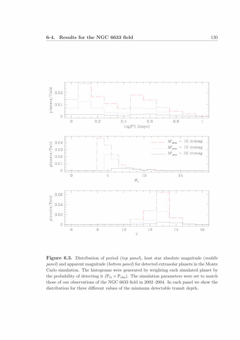
6-4. Results for the NGC 6633 field 130
Figure 6.3. Distribution of period (top panel), host star absolute magnitude (middlepanel) and apparent magnitude (bottom panel) for detected extrasolar planets in the MonteCarlo simulation. The histograms were generated by weighting each simulated planet bythe probability of detecting it (Ptr × Pobs). The simulation parameters were set to matchthose of our observations of the NGC 6633 field in 2002–2004. In each panel we show thedistribution for three different values of the minimum detectable transit depth.

6-5. Increasing the detection rate 131
0.03 planets per field (2 complete transits). The reduced estimate, relative to the
NGC 6633 case, is due to the smaller number of images, fewer nights with long
continuous coverage (mostly due to bad weather), and sparser time sampling. Thus
our estimate of the total planet catch in these 8 fields is ∼ 0.3 planets, or ∼ 0.6 if
we settle for one complete detected transit (plus at least one partial one).
This disappointing estimate suggests that our initial strategy of simultaneously
monitoring four fields over multiple seasons is not optimal. We selected this strategy
believing it would maximise the number of stars we monitor, while obtaining a
minimum time-sampling required to detect a transit (one image every ∼ 14 minutes).
The signal-to-noise ratio of a detection would be increased by folding the lightcurve
at the appropriate period. However, gaps in the observations due to weather and
technical problems have reduced the probability of detecting multiple, complete
transits (Fig. 6.1). The systematic trends present in many of the lightcurves have
prevented us from using software to make shallow transits detectable by phase-
folding. In the present data, individual and partial transits need to be detectable
before a period can be determined. Therefore we have updated our strategy to
increase the cadence of our observations.
6-5 Increasing the detection rate
Using the tool we have developed, we can simulate a number of alternative observing
strategies. This way we can not only improve our detection rate, but also predict
how the properties of the detected systems might depend on the chosen strategy.
The main parameters we varied were the choice of filter, the Galactic latitude of
target fields, and observing schedule. We tested what we might gain from being
able to detect shallower transits. The results are summarised in Table 6.1.

6-5. Increasing the detection rate 132
Table 6.1. Estimated planet catch for various simulated observing strategies, and forour observations of the NGC 6633 field (cases A–C). Each case is parametrised by thewavelength band used, the Galactic latitude (b) of the target fields, the number of completeobserving nights (Nnt), the number of hours observed per night (Tnt), and the cadence (C,images per hour). The total number of images (Nim) is generally less than Nnt × Tnt × C
because of the change in the rise and set times of the field over the course of the run.Ndet is the estimated number of detections per APT field, shown for one or two completeobserved transits. Except for cases B and C, the transit depth threshold (∆Fmin) is10 mmag. Cases 1–10 are based on the same simulated observing schedule. Scheduleswith the same parameters but random gaps at different times yield the same Ndet valuesto within ±0.01.
Case Band |b| Nnt Tnt C Nim Ndet(1) Ndet(2) Comments
A V 8 61 1–7 4–16 2486 0.22 0.12 ∆Fmin = 10 mmag
B V 8 61 1–7 4–16 2486 0.09 0.05 ∆Fmin = 15 mmag
C V 8 61 1–7 4–16 2486 0.02 0.01 ∆Fmin = 20 mmag
1 V 0 20 8 15 2147 0.23 0.16
2 V 15 20 8 15 2147 0.22 0.16
3 V 90 20 8 15 2147 0.16 0.11
4 I 0 20 8 15 2147 0.26 0.20
5 I 8 20 8 15 2147 0.25 0.19
6 I 15 20 8 15 2147 0.27 0.20
7 I 25 20 8 15 2147 0.26 0.20
8 I 45 20 8 15 2147 0.22 0.16
9 I 65 20 8 15 2147 0.21 0.16
10 I 90 20 8 15 2147 0.19 0.14
11 I 15 20 10 15 2782 0.36 0.30
12 I 15 16 10 15 2221 0.28 0.23
13 I 15 20 6.5 15 1863 0.22 0.15
14 I 15 26 6.5 15 2349 0.29 0.21
15 I 15 10 8 15 1163 0.12 0.08
16 I 15 30 8 15 2990 0.38 0.29
17 I 15 20 8 30 4346 0.43 0.32
18 I 15 20 8 7.5 1081 0.13 0.10
19 I 15 20 8 15 2300 0.30 0.22 no gaps
20 I 15 20 10 15 2888 0.39 0.31 no gaps

6-5. Increasing the detection rate 133
Figure 6.4. Dependence of the total planet catch on the minimum detectable transitdepth. Ndet(2) is the number of detections per APT field with two complete observedtransits. Four cases are shown: our observations of the NGC 6633 field, the same fieldobserved in V and I with a model observing schedule containing 20 nights of observations,and this model schedule but targeting a higher Galactic latitude in I band.
6-5.1 Minimum detectable transit depth
The sharp cutoff in MV , beyond which stars are too large to have detectable transits
(Fig. 6.3, middle panel), is a strong function of the assumed planet size (Rp) and the
minimum detectable transit depth (∆Fmin). The overall detection rate also depends
significantly on these parameters because most of the detected planet hosts are near
this cutoff. As ∆F is proportional to Rp2, varying Rp
−2 should have the same effect
as varying ∆Fmin.
Figure 6.4 shows how the detection rate varies with ∆Fmin for a number of observ-
ing strategies. Observations in the I band are less sensitive to ∆Fmin, as in those
cases redder stars with deeper transits make up a larger fraction of the detected

6-5. Increasing the detection rate 134
host population (Fig 6.9). For the same reason, as long as ∆Fmin is no smaller than
∼ 10 mmag, observations in the I band will always detect more planets (Sec. 6-5.3).
Any gain from the ability to detect transits shallower than this is almost entirely
due to planets around larger, bluer stars, and therefore is more significant in the V
band and at low Galactic latitude.
This last comment assumes that planets around early-type stars are equally fre-
quent. Little is known about planets around these stars. Radial velocity searches
generally target stars of spectral type late F to M (e.g. Lineweaver & Grether 2003).
The simulation indicates that if we can ensure that 5 mmag transits are routinely
detectable in our search, we will be sensitive to planets around stars as large as
A5. This further motivates attempts to remove systematics from the lightcurves.
However, a search for planets around such stars would need to target the Galactic
plane (as that is where the early-type stars are concentrated, see Fig. 6.9). As will
be seen below, this is not optimal for a planet search in general.
6-5.2 Observing schedule
We generated possible sets of observing epochs, parametrised by the maximum
length of continuous observations per night (Tnt), the total number of full observ-
ing nights (Nnt), and the cadence or sampling frequency (C, number of images per
hour). In order to make these as realistic as possible, we have included gaps due to
bad weather (giving each night a slightly pessimistic 50% probability of yielding no
observations), and due to Full Moon (7 days). We have also included the effect of
the changing rise and set times of a field over the course of the run due to sidereal
motion. This slightly reduces the actual duration of observations below Tnt on nights
at the beginning and/or end of the run, especially for longer runs.
In I band, we have found that an exposure time of 60 sec reaches a reasonable
magnitude limit (Fig. 3.3). Including CCD readout, pointing correction, and slewing
to an adjacent field, we can obtain just over 30 images per hour. If we observe two
fields alternately, we obtain a cadence of 15/h for each field, which is about ideal.

6-5. Increasing the detection rate 135
We could observe twice as many simultaneous fields at half the cadence, giving half
the detection rate per field (compare cases 6 and 18 in Table 6.1), but the reduced
sampling frequency would make transit candidates more difficult to characterise (e.g.
Seager & Mallen-Ornelas 2003). Concentrating on a single field and obtaining 30
images per hour (case 17) would, on the other hand, reduce the overall detection
rate. Therefore 15/h is a good compromise. In V band, the longer exposure time
(150 sec) means we can only obtain this cadence (actually almost 17/h) by observing
one field at a time.
At Siding Spring Observatory, the minimum number of dark hours per night is
6.5 (in December and January). For 8 months of the year, we have at least 8 h
per night, while a minimum of 10 h per night is available for 4 months of the year.
Targeting a field at a declination south of −40, we can observe at an airmass below
2 for at least 10 h. Presently, the APT can only continuously track an object for
a little over 8 h, due to a safety limit switch on the right-ascension axis. However,
physical limitations do not prevent the telescope from reaching hour angles up to
±6 h. With slight hardware modifications to ensure the safety of the telescope, the
restriction can be relaxed, allowing longer observations. These modifications are
currently under way. For the simulations with Tnt = 10 h, we have assumed that a
field can be tracked for 10 h, while for those with shorter Tnt we used the current
8 h limit.
The effect of Tnt on the detection probability (Pobs) is shown in Figures 6.5 and 6.6,
and highlights the importance of observing continuously for as long as possible each
night (e.g Mallen-Ornelas et al. 2003). This is primarily because of our requirement
to detect complete transits. Note that Pobs is only a measure of the phase coverage,
and is independent of other factors, such as the geometric transit probability and
the distribution of orbital periods. For the effect on the overall detection probability,
compare cases 11 and 13 (Table 6.1). If we are able to observe for 10 hours each
night, we will detect 50% more planets than we would in the same number of 8 hour
nights. If Nnt is adjusted to give the same total number of images (cases 12 and 14),
approximately the same detection rate is achieved.

6-5. Increasing the detection rate 136
Comparing Figures 6.5 and 6.6 also demonstrates the effect of gaps in the
lightcurves. For a fixed number of photometric nights (Nnt), the lightcurves with
gaps are longer than Nnt days. This makes the dips in Pobs near periods that are
multiples of a day narrower (because periods have to be closer to an integer number
of days to avoid detection). Also, some non-integer periods that are too long to
be detectable in 20 consecutive nights become detectable when those nights span a
longer duration. The overall planet catch is only slightly reduced by gaps (compare
case 19 to case 6, and case 20 to case 11 in Table 6.1). In fact, gaps can even in-
crease the phase coverage at small values of Nnt, where the increased time span has
a more significant effect (Fig. 6.7). However, as Mallen-Ornelas et al. (2003) point
out, the period of a detected signal is more likely to be incorrectly determined from
a lightcurve with gaps.
Without running the full simulation, we can determine the optimal number of
nights (Nnt) to observe a field using the approach of Mallen-Ornelas et al. (2003).
Averaging Pobs over the period range of interest gives a measure of the overall ef-
ficiency (purely from a phase-coverage point of view) of an observing schedule.5
<Pobs > is plotted against run length in the upper panels of Figures 6.7 and 6.8.
Obviously <Pobs > is an increasing function of the run length. However, the ef-
ficiency of the observing run, defined as <Pobs >/Nnt, reaches a maximum value,
beyond which the gain from additional nights of observing begins to decrease (see
the lower panels). The optimum number of nights is about 20 for 8 hour nights, or
15 if 10 hours of continuous observations are possible. Though <Pobs > is reduced
by missing nights in the lightcurves, the optimum Nnt values appear to be the same
as if no gaps were present.
Comparing cases 11 and 12 (both with Tnt = 10 h, see Table 6.1) suggests that
the optimum Nnt values just derived are somewhat underestimated, as the value
of Ndet(2)/Nnt is in fact slightly higher for Nnt = 20, than at Nnt = 16. This can
be explained by the fact that the calculation of <Pobs > was weighted in favour of
5 Mallen-Ornelas et al. (2003) averaged Pobs over the period range 3–4.5 d, presumably sampledat even intervals in period. We used the full 1–9 d range, but sampled it evenly in log(P ), givingmore weight to the shorter periods.

6-5. Increasing the detection rate 137
Figure 6.5. The phase coverage factor in the detection probability as a function ofthe period and the duration of continuous coverage per night. Pobs is the probability ofobserving at least two complete transits (with a typical 0.1 day duration) with at least100 in-transit points. All model lightcurves used here have a cadence of 15 images perhour, and contain 20 consecutive nights of observations.
shorter periods, while in the simulation, planets with periods in the range 1–3 d are
only 15% as frequent as those with 3–9 d periods.
6-5.3 Choice of filter
Observing at a red wavelength, in particular in I band, has a number of advantages
for a transit search (e.g. von Braun et al. 2005). The pros and cons of using this filter
are summarised in Section 7-2.1. We used our simulations to compare (otherwise
identical) strategies using V and I filters.
The I-band absolute magnitudes (MI) of simulated stars were obtained from their
MV values and V − I colours for main sequence stars tabulated in Cox (2000). The

6-5. Increasing the detection rate 138
Figure 6.6. Same as Fig. 6.5, but for more realistic lightcurves with gaps due to weatherand Full Moon (20 full nights of observations).
interstellar extinction is about half what it is in V band (Cox 2000), thus a value of
1 mag/kpc was used in the calculation of apparent I magnitudes. The parameters
of the noise model were also adjusted to match those observed in our 60 sec I-
band images, namely a sky flux of 4000 ADU/pixel, and a magnitude zero-point of
21.9 mag.
One significant advantage of using the I band is that it significantly increases the
number of well-measured red dwarf stars in our sample (which have deeper potential
transits) relative to their larger, bluer counterparts. This is illustrated in Figure 6.9.
We made the comparison between observations in V and I at three Galactic
latitudes (cases 1–3 and 4, 6, 10 in Table 6.1). The number of detections per field
for identical observing schedules is already slightly greater in the I band. However,
as pointed out above, at the cadence assumed here, we can observe two fields in

6-5. Increasing the detection rate 139
Figure 6.7. Top panel: Average phase coverage as a function of the total number ofnights in an observing run. Pobs (as defined in the caption of Fig. 6.5) is averaged overthe period range 1–9 d (sampled logarithmically). Each night is close to 8 hours long(subject to sidereal motion, see text). The cadence is 15 images per hour. The dashedline is the ideal case of Nnt consecutive nights. The solid line is for more realistic modellightcurves, with gaps (entire nights) due to bad weather and Full Moon. Bottom panel:A measure of the efficiency of a run, <Pobs >/Nnt, as suggested by Mallen-Ornelas et al.(2003). After about 20 nights, more detections will result from moving to a new field thanfrom continued observations on the same field.
parallel in I, but only one in V . Therefore we increase our detection rate by more
than a factor of 2 by observing in I.
6-5.4 Galactic latitude
The main relevance of the Galactic latitude targeted is in determining the level of
crowding in the field, and thus the probability of planetary transit signals being
diluted by blended stars (Fig. 6.10). It also has an effect on the distribution of the
spectral types of the stars we measure (Fig. 6.9). At high Galactic latitude, we begin
to lose the more distant F and G stars (MV ≈ 4). As the reddest stars are only

6-5. Increasing the detection rate 140
Figure 6.8. Same as Figure 6.7, but for 10 hour nights. In this case the most efficientrun is somewhat shorter, about 15 nights.
seen within ∼ 100 pc in our magnitude-limited sample, their numbers (and thus the
number of detections they yield) are essentially independent of the latitude.
The overall detection rate is essentially constant from the Galactic plane out to
at least |b| ≈ 25. Even at the Galactic pole, it is only ∼ 30% lower (see cases 4–10
in Table 6.1).
The level of crowding is relevant for two other of reasons. Firstly, it has an
effect on the photometric precision (Sec. 2-2.17) and the occurrence of systematic
errors (Sec. 3-5), neither of which is considered in our simulations. This means the
signal-to-noise ratios we calculate are generally slightly optimistic, but more so in
crowded fields. Second, although we have not simulated “false alarm” detections
due to blended eclipsing binaries (Sec. 1-6.4), it is clear that the frequency of these
will be strongly correlated with the crowding.
For the above reasons, we conclude that we should avoid the Galactic plane
itself. Fields at |b| ≈ 25 are optimal. Considering also the need for some flexibility

6-5. Increasing the detection rate 141
Figure 6.9. Left panels: The effect of the filter used on the absolute magnitude dis-tribution of stars that may host detectable planets. We approximate this population byselecting stars brighter than magnitude 13.5 (in both V and I), and whose flux is mini-mally diluted (fap > 0.9). The magnitude limits are the approximate magnitudes of thefaintest stars leading to detections in our simulations (see the bottom panels of Figures 6.3and 6.11). Right panels: The effect on the distribution of host stars of detected planets(assuming all stars are equally likely to have a planet, and ∆Fmin = 10 mmag), in a sim-ulated 20-night observing run. The comparison is made at two Galactic latitudes (cases2, 3, 6 and 10 in Table 6.1).

6-6. Discussion 142
Figure 6.10. A measure of the amount of blending in an APT image, as a function ofthe Galactic latitude of the field, based on our simulated stellar populations. fap is thefraction of the total starlight in a photometry aperture coming from a single star. Thephotometry apertures are 3 pixels (∼ 28′′) in radius. Here fap is averaged over all objects(possibly blends) with total apparent brightness I < 13.5 or V < 13.5.
in choosing fields throughout the year, our future targets will be in the range 15 <∼|b| <∼ 45.
6-6 Discussion
We have constructed a simple model to simulate a population of stars observed in
an APT field. Combined with some basic assumptions on the detectability of transit
signals, and the set of epochs at which we sampled the lightcurves, we have estimated
the total number of planets we expect to detect in the first 8 fields we observed.
Even with the most optimistic parameters, this number is only ∼ 0.6, and a more
realistic figure could be an order of magnitude smaller. Although disappointing, our
estimate is consistent with the fact that we have not yet detected any planets, and
highlights the fact that our initial strategy was far from optimal.
We can also combine the stellar model with simulated sets of sampling times to
determine how the observing strategy can be improved. Our detailed study of the

6-6. Discussion 143
effects of various observing parameters has led to the following ways to maximise our
detection rate (some of which have also been noted by other transit-search teams):
1. Observe in I band;
2. Target fields in the range 15 <∼ |b| <∼ 45;
3. Maximise the duration of continuous observations each night;
4. Select new fields after every 20–30 full nights of observations;
5. Observe two fields in parallel, obtaining 15 images per hour of each.
Applying this new strategy, we can detect the same 0.6 planets in a little over
20 nights of observations (multiply Ndet(1) of case 6 or 7 in Table 6.1 by two). In
fact we can even slightly exceed this rate, once we are able to observe for 10 hours
continuously (case 11). These estimates apply even if 50% of nights are taken out
by bad weather (and we don’t observe in bright time), and thus the 20 nights take
about 2 months to accumulate. Figure 6.11 shows some basic properties of systems
detected by this strategy.
Observing 5 pairs of fields per year (each for 2 months, allowing for telescope
downtime or use for other projects) will lead to an overall detection rate of up
to 2–3 planets per year. This is an order of magnitude greater than the estimate
for our 2002–2004 observations. A further significant increase will result from the
installation of the new CCD camera being built in 2005 (Sec. 7-3.3).
An important advantage of the new observing strategy we have chosen is that
candidates can be selected in a relatively short time. This allows follow-up studies to
be conducted immediately, while the candidates are still observable and the orbital
phase information obtained from the lightcurves is precise.
Due to our simplifying assumptions and incomplete knowledge of the properties
and frequency of extrasolar planets, the absolute detection rates calculated here are
uncertain by a factor of a few. However, our conclusions regarding the improvement
of our search are mostly based on the relative detection rates of various strategies,

6-6. Discussion 144
Figure 6.11. Distribution of period (top panel), host star absolute magnitude (middlepanel) and apparent magnitude (bottom panel) for detected extrasolar planets, for a modelof our optimal observing strategy (compare to the results for our NGC 6633 data, shownin Fig. 6.3). The effect of the assumed minimum detectable transit depth are shown. Weare confident that with future improvements in trend filtering, the ∆Fmin = 10 mmag casewill become a realistic one.

6-6. Discussion 145
which should not be strongly affected by these uncertainties. Further refinement
of the simulations, such as a more detailed model of the stellar populations in the
Galaxy (including non-main-sequence stars), would make the results more realistic
and reduce some of the uncertainty, but would not alter our present conclusions
significantly.
Another limitation of the analysis given in this chapter is that we have only con-
sidered the detection of transit signals due to planets. For each such detection, there
will be numerous additional candidates due to binary stars (Sec. 4-2), which need
to be eliminated. The considerable amount of follow-up observations required for
the confirmed detection of a planet lead to additional biases in the overall sensitiv-
ity of our search. A detailed analysis of these biases is beyond the scope of this
thesis. In broad terms, the probability of obtaining spectroscopic confirmation will
be an increasing function of planet mass and host star apparent brightness, but will
decrease with increasing host mass and orbital period. Planets in multiple stellar
systems may also be more difficult to confirm spectroscopically.

Chapter 7
Conclusions & Future Work
7-1 Summary of results so far
This thesis work has been primarily focused on setting up a search for transiting ex-
trasolar planets using the Automated Patrol Telescope. Largely automated methods
for the collection, reduction and analysis of data were developed. Reaching the high
photometric precision required for such a search has been a significant challenge.
It required the development of a new observing technique, and the selection and
adaptation of appropriate data reduction software.
The first observations using the new technique were taken in August 2002, and
in the two years that followed, a significant volume of data was collected on 8 main
fields. We have analysed the best of these data and selected a number of tentative
planet candidates. We focused mainly on the field centred on the open cluster
NGC 6633, for which we had the highest quality lightcurves. These yielded four
planet candidates, as well as a list of variable stars and eclipsing binary systems.
We found one additional candidate in each of 3 other fields, though two of these
were discarded based on spectral types obtained from an online catalogue.
None of the 5 remaining candidates were particularly promising, having larger
estimated radii than those of the few known transiting exoplanets. Indeed, follow-up
observations have identified each of them as binary stars. However, we have gained
7-1. Summary of results so far 147
valuable experience from the exercise, and demonstrated our ability to efficiently
follow up candidates with photometry and spectroscopy.
The ultimate goal of this work is the detection and characterisation of new extra-
solar planets. In this it has not yet been successful, and therefore has not contributed
to our understanding of extrasolar planets. The most potent statement we can make
is that our calculated detection rate, based on current knowledge of the properties
of these systems, is consistent with our lack of detections so far. We identify three
main reasons for this low detection rate.
• Our initial choice of observing strategy was far from optimal.
• Numerous gaps in the lightcurves due to problems with the telescope and camera.
• Systematic errors in the photometry, preventing the effective use of transit de-
tection software.
We have updated our observing strategy, and have been obtaining higher quality
lightcurves since November 2004. Details are given in the following section.
Many of the technical difficulties have been dealt with, and the APT is now
a highly reliable instrument. Some downtime is expected in late 2005 during the
commissioning of the new camera (Sec. 7-3.3), but the benefits of the new instrument
will far outweigh the lost observing time.
A mechanical problem responsible for some of the systematics (Sec. 3-5) has been
largely solved, and great care will be taken to avoid such a problem with the new
camera. New data are now processed within a few days of being taken, and the
lightcurves are inspected weekly, so if similar problems do arise in the future, they
will be detected and corrected more promptly.
At present, some artificial trends in the lightcurves are still observed, and do limit
our ability to detect shallow transit signals. However, a recently published trend
filtering algorithm (Kovacs, Bakos & Noyes 2004) offers an effective way of greatly
reducing these limitations.

7-2. The way ahead 148
So while we have not yet reached our goal of detecting planets, we have already
addressed some of the reasons for this, and we can describe a clear way ahead. Our
project is finally reaching maturity. Being optimistic, but not overly so, we can hope
to make our first detection in the next year.
7-2 The way ahead
With the benefit of experience gained from our first two years of observations, and
insights from the simulations described in Chapter 6 and the reports of other transit
search teams, we have updated our observing strategy. The new strategy is optimal
in that it maximises our potential detection rate, while keeping the frequency of
false-positive detections (binary stars) to a minimum.
7-2.1 Choice of filter
All future observations will be made in I band. In fact, we have been observing in
this band since August 2004. The advantages of using I band, compared to shorter
wavelengths (in particular V band), are summarised below.
• Planets orbiting small, red stars are more likely to cause transits deep enough
to be detectable. These stars appear brighter in I band, and therefore more
of them are measured with sufficient precision to make their transits detectable
(see Fig. 6.9).
• The effect of limb-darkening decreases with wavelength. This makes planetary
transits more flat-bottomed, and thus easier to distinguish from grazing eclipses
of binary stars (e.g Seager & Mallen-Ornelas 2003).
• Interstellar extinction is lower in I, allowing small, intrinsically faint stars to be
seen at slightly greater distances (e.g. von Braun et al. 2004)1
1 This is only an advantage for fields away from the Galactic plane. In the plane, the reduced ex-tinction makes distant background stars brighter, leading to more frequent blending and a brighterand more noisy background.
7-2. The way ahead 149
• Atmospheric extinction is lower in I band, reducing any residual trends in the
lightcurves due to the variation of airmass over the course of a night, and across
the field of view.
• The quantum efficiency of our CCD is highest in I band, allowing shorter expo-
sure times, and thus more fields can be observed in parallel (or the same number
at higher cadence).
• The amplitude of the CCD intra-pixel sensitivity variations is smaller at longer
wavelengths (Sec. 2-2.12). While the limit imposed on the photometric precision
by these variations is greatly reduced by the raster-scan technique even in the V
band (Sec. 2-4.1), some residual effect may still contribute to the noise for the
brightest stars.
There are also disadvantages to observing in I band.
• The sky is considerably brighter than in V band.
• A significant part of the I-band sky brightness is due to OH emission lines, whose
strength varies spatially (over angles of ∼ 1) and in time (over timescales of
minutes).
• Fringing caused by reflections and interference in the CCD structure is more
likely to have a significant effect in I band, due to the existence of night sky
emission lines in that wavelength range.
• The shorter exposure time (∆t) increases the scintillation limit, which is propor-
tional to ∆t−1/2 (see Equation 2.2). At an airmass of 1.5, the limit is ∼ 1.5 mmag
per image (60 sec exposure).
We have not observed any fringing in our images. Figure 3.3 shows that the
variability of the I-band sky brightness does not have a significant effect on the
photometry. The noise model in our simulations (Sec. 6-2) included the observed
sky brightness, and a limiting precision of 1.5 mmag, and predicted significantly

7-2. The way ahead 150
higher detection rates for I-band observations than those in V . Therefore we believe
that I band is the best choice.
Another possible advantage of using I band is that the sky at Full Moon is only
about twice as bright as it is when the Moon is down (because a significant part of
this sky brightness is due to the OH lines). Though we have not yet explored this
possibility, we may be able to obtain up to an extra 7–8 nights of useful data per
lunar cycle, increasing our phase coverage and thus the efficiency of our search.
7-2.2 Field selection
We have established in the previous chapter that we should target Galactic latitudes
in the range 15 <∼ |b| <∼ 45, with the optimal fields being near |b| = 25. This will
maximise the detection rate while limiting the number of false-alarms due to blended
binary stars.
Additionally, we need to select fields that are observable at low airmass for as
long as possible each night, i.e. fields at southern declinations (δ). All fields at
δ < −9 are at an airmass below 2 for at least 8 hours per night. To benefit from
our future ability to observe a field continuously for up to 10 hours (Sec. 7-3.2), our
fields will need to be at δ < −40.
Targeting fields closer to the celestial pole has the slight advantage of decreasing
the range of airmass variation over the night (though increasing its minimum value).
This would help reduce any extinction-related trends in the data. The telescope
mount imposes a southern declination limit of −70.
The above considerations leave us sufficient flexibility to have potential fields
observable throughout the year.
7-2.3 Observing schedule
Based on our analysis in Chapter 6 we have selected a more appropriate observing
schedule for our search. This analysis has taken into account observing time lost due

7-2. The way ahead 151
to weather and Full Moon. The goal is to intensively observe a field so that sufficient
data are accumulated for a reasonable detection rate in a relatively short observing
run. This allows a large number of fields to be monitored over the course of a year,
and candidates can be followed up within a month or two of being detected. Also,
because the lightcurves are well sampled, individual transits are detectable and the
search is less reliant on the ability to increase the signal-to-noise ratio by phase-
folding the lightcurves (Mallen-Ornelas et al. 2003). This is an advantage because
it reduces the effect of systematic trends on the detection probability.
We want to observe at high cadence in order to maximise the signal-to-noise
ratio of individual transits in the lightcurve, and to better characterise their shapes.
We can reach a reasonable compromise between this and maximising the number
of target stars by observing two fields in parallel in I band. With 60 s exposures,
we obtain 15 images per hour for each field. An alternative which we have not
yet investigated in detail, would be to concentrate on a single field and take longer
exposures. However, this possibility is limited by the fact that fainter candidates
are more difficult to follow up. Also, because in a 60 s I-band image the average sky
flux per pixel is already ∼ 10% of the full-well level, increasing the exposure time
will push a disproportionate number of stars above the saturation limit.
On every clear night, we will observe the current fields continuously for the max-
imum possible duration. At present this is limited to ∼ 8 hours by the telescope
hour-angle limit, but will soon be extended to at least 10 hours (Sec. 7-3.2). Once
we have observed a pair of fields on 20–30 full nights (or about two months in to-
tal time), we will select new fields, as the efficiency of the observing run (planets
detected per night) decreases beyond this point.
Our data reduction pipeline can generate lightcurves essentially in real time, al-
lowing us to use an additional strategy suggested by von Braun et al. (2004). These
authors point out that if no single transits are detected in the first 10 nights of data
on a field (which is about half the optimum run length in their case, as well as ours),
the the probability of detecting multiple transits in an additional 10 nights (or even
20) is less than the probability of making such detections in 20 nights on a new field.

7-3. Hardware upgrades for the APT in 2005 152
Thus we can search the lightcurves about half-way through the optimum run length
and decide whether continued observations on a field are worthwhile. Of course, this
depends on our ability to reliably detect individual transits in the lightcurves.
7-2.4 Data reduction and analysis
A number of improvements to our data reduction and analysis procedures are also
possible. Further experiments with optimising the photometry aperture size (and
shape) could reduce the noise and systematic errors in the lightcurves of blended
stars (Sec. 2-5.6). However, as we are now observing less crowded fields than previ-
ously, the overall gain from this may be minimal. More importantly, further work is
needed in investigating the sources of systematic trends in our lightcurves (Sec. 3-5),
and ways of removing or minimising them. Efforts to improve the sky-subtraction
algorithm will be a part of this.
It is unlikely that all the causes of the systematics can be identified and removed.
Therefore one priority is to complete our implementation of the Kovacs et al. (2004)
trend filtering algorithm (Sec. 4-1.3). Once this is done, we can turn our attention to
the transit detection software of Aigrain & Irwin (2004), fine-tuning its parameters
and evaluating its sensitivity to signals in our data.
7-3 Hardware upgrades for the APT in 2005
7-3.1 Full Automation
All the tasks involved in observing with the APT are already automated, and can
be orchestrated by simple scripts (Sec. 2-1.1). The control PC has the ability to
automatically close the roof in the event of rain or other conditions that could
damage the telescope. At present, these safety measures are not fully reliable, and
thus an observer must monitor the telescope and weather conditions over the entire
night. Additional measures will eventually remove this necessity, and allow regular
7-3. Hardware upgrades for the APT in 2005 153
observations to be conducted without human intervention. Considering the exten-
sive observations required for the planet search project, this will be an important
improvement at least from a practical point of view. It may also make the search
more efficient, as gaps in the observations due to a lack of available observers, will
no longer occur.
7-3.2 Extended hour-angle range
As discussed in Section 6-5.2, it would be highly advantageous to be able to exceed
the APT’s current hour-angle limit of ±4 h. This requires the relocation of a number
of limit switches on the telescope mount, and the installation of some additional
security measures to ensure that the telescope cannot be damaged by hitting a
physical limit. Work has already begun on the first stage of this process, which
will allow the telescope to reach hour angles up to ±5 h. We expect to complete
this stage in March 2005. Further modifications may allow even higher hour angles
to be reached. The maximum duration of continuous observations at the APT is
ultimately limited to ∼ 11 h by the number of dark hours (in June–July). However,
having a greater hour-angle range increases our flexibility in the choice of fields (in
right ascension, at the expense of declination: we have to go further south to keep
the airmass low at high hour angles).
7-3.3 A new camera for the APT
A new CCD camera is being designed and built at the Anglo Australian Observatory,
and is due to be installed on the APT in early 2006. It will use a pair of MITLL
chips with 6k × 3k pixels each. The pixels are 10 µm in size, giving an image scale
of 4.19 arcseconds per pixel. The two chips will cover a square field ∼ 7 across.
The effective field of view will be set by the field-flattening optics. A model of the
telescope optics2 suggests that a suitable point spread function will be obtained at
2 The telescope optics were modelled using ZEMAX software (a registered trademark of ZE-MAX Development Corporation; http://www.zemax.com/zemax/). The figures quoted here were

7-3. Hardware upgrades for the APT in 2005 154
least within 2.5 degrees of the optical axis. Depending on the final camera design,
the usable field of view may be 3 in radius, or even slightly larger. The new field
area will thus be 3–5 times larger than the current one, increasing our detection rate
by the same factor.
The new CCDs will also have about twice the quantum efficiency of the current
one reducing the exposure times. The readout time for the full chips is expected to
be ∼ 20 seconds, but because the useful part of the field will be significantly smaller,
only a part of each chip will need to be read out. Therefore we will be able to obtain
higher cadence observations than at present. With the smaller pixel size, the images
will be only slightly undersampled (Sec. 2-2.8). This will improve the photometric
precision, and reduce the effects of blending. The combination of these advantages
will further increase our potential detection rate.
obtained from the model by J. Everett.

References
Agol E., Steffen J., Sari R., Clarkson W., 2005, MNRAS, submitted (astro-ph/0412032)Aigrain S., Favata F., Gilmore G., 2004, A&A, 414, 1139Aigrain S., Irwin M., 2004, MNRAS, 350, 331Alcock C., Allsman R. A., et al., 1997, ApJ, 486, 697Allen C. W., 1973, Astrophysical Quantities, third edn. Athlone Press, LondonAlonso R., Brown T. M., et al., 2004, ApJ, 613, L153Andersen J., 1991, A&AR, 3, 91Anderson J., King I. R., 2000, PASP, 112, 1360Angel J. R. P., 1994, Nat, 368, 203Ardila D. R., Golimowski D. A., et al. 2004, ApJ, 617, L147Armitage P. J., Livio M., Lubow S. H., Pringle J. E., 2002, MNRAS, 334, 248Artymowicz P., Lubow S. H., 1994, ApJ, 421, 651Arzoumanian Z., Joshi K., Rasio F. A., Thorsett S. E., 1996, in ASP Conf. Ser.. p. 525Bakos G., Noyes R. W., Kovacs G., Stanek K. Z., Sasselov D. D., Domsa I., 2004, PASP,
116, 266Bally J., Testi L., Sargent A., Carlstrom J., 1998, AJ, 116, 854Barnes J. W., Fortney J. J., 2004, ApJ, 616, 1193Beer M. E., King A. R., Pringle J. E., 2004, MNRAS, 355, 1244Beichman C., 2000, in ESA SP-451: Darwin and Astronomy : the Infrared Space Inter-
ferometer. p. 239Beichman C., Gomez G., Lo M., Masdemont J., Romans L., 2004, Advances in Space
Research, 34, 637Beichman C. A., Bryden G., et al. 2005, preprint (astro-ph/0412265)Bender P. L., Stebbins R. T., 1996, J. Geophys. Res., 101, 9309Benedict G. F., McArthur B., et al. 1999, AJ, 118, 1086Bodenheimer P., Hubickyj O., Lissauer J. J., 2000, Icarus, 143, 2Bond I. A., Abe F., et al., 2001, MNRAS, 327, 868Bond I. A., Udalski A., et al. 2004, ApJ, 606, L155Borde P., Rouan D., Leger A., 2003, A&A, 405, 1137Borucki W. J., Caldwell D., Koch D. G., Webster L. D., Jenkins J. M., Ninkov Z., Showen
R., 2001, PASP, 113, 439Borucki W. J., Koch D. G., et al., 2003, in ASP Conf. Ser. 294: Scientific Frontiers in

References 156
Research on Extrasolar Planets. p. 427Boss A. P., 1997a, Bulletin of the AAS, 29, 1254Boss A. P., 1997b, Science, 276, 1836Boss A. P., 1998a, ApJ, 503, 923Boss A. P., 1998b, Bulletin of the AAS, 30, 1057Boss A. P., 2000, ApJ, 536, L101Boss A. P., 2001, ApJ, 563, 367Boss A. P., 2002a, ApJ, 576, 462Boss A. P., 2002b, ApJ, 567, L149Boss A. P., 2003, ApJ, 599, 577Boss A. P., Wetherill G. W., Haghighipour N., 2002, Icarus, 156, 291Bouchy F., Pont F., Melo C., Santos N. C., Mayor M., Queloz D., Udry S., 2005, A&A,
accepted (astro-ph/0410346)Bouchy F., Pont F., Santos N. C., Melo C., Mayor M., Queloz D., Udry S., 2004, A&A,
421, L13Bracewell R. N., 1978, Nat, 274, 780Bracewell R. N., MacPhie R. H., 1979, Icarus, 38, 136Brown T. M., 2001, ApJ, 553, 1006Brown T. M., 2003, ApJ, 593, L125Brown T. M., Charbonneau D., Gilliland R. L., Noyes R. W., Burrows A., 2001, ApJ, 552,
699Bruntt H., Grundahl F., Tingley B., Frandsen S., Stetson P. B., Thomsen B., 2003, A&A,
410, 323Buffington A., Booth C. H., Hudson H. S., 1991, PASP, 103, 685Bundy K. A., Marcy G. W., 2000, PASP, 112, 1421Burke C. J., Depoy D. L., Gaudi B. S., Marshall J. L., 2003, in ASP Conf. Ser.. p. 379Burrows A., Hubeny I., Hubbard W. B., Sudarsky D., Fortney J. J., 2004, ApJ, 610, L53Butler R. P., Bedding T. R., Kjeldsen H., McCarthy C., O’Toole S. J., Tinney C. G.,
Marcy G. W., Wright J. T., 2004, ApJ, 600, L75Butler R. P., Marcy G. W., Vogt S. S., Fischer D. A., Henry G. W., Laughlin G., Wright
J. T., 2003, ApJ, 582, 455Cameron A. G. W., 1962, Icarus, 1, 13Cameron L. M., 1985, A&A, 147, 39Canup R. M., Righter K., et al. 2000, Origin of the earth and moon. Tucson: University
of Arizona Press; Houston: Lunar and Planetary InstituteCarter B. D., Ashley M. C. B., Sun Y.-S., Storey J. W. V., 1992, Proc. ASA, 10, 74Charbonneau D., Brown T. M., Dunham E. W., Latham D. W., Looper D. L., Mandushev
G., 2004, in AIP Conf. Proc. 713: The Search for Other Worlds. p. 151Charbonneau D., Brown T. M., Latham D. W., Mayor M., 2000, ApJ, 529, L45Charbonneau D., Brown T. M., Noyes R. W., Gilliland R. L., 2002, ApJ, 568, 377Charbonneau D., Noyes R. W., Korzennik S. G., Nisenson P., Jha S., Vogt S. S., Kibrick

References 157
R. I., 1999, ApJ, 522, L145Chromey F. R., Hasselbacher D. A., 1996, PASP, 108, 944Clarkson W. I., Christian D. C., et al 2004, AAS Meeting Abstracts, 205,Collier Cameron A., Horne K., Penny A., James D., 1999, Nat, 402, 751Correia A. C. M., Udry S., Mayor M., Laskar J., Naef D., Pepe P., Queloz D., Santos
N. C., 2004, preprint (astro-ph/0411512)Coustenis A., et al. 1997, in ASP Conf. Ser. 119: Planets Beyond the Solar System and
the Next Generation of Space Missions. p. 101Coustenis A., Schneider J., et al. 1998, in ASP Conf. Ser. 134: Brown Dwarfs and Extra-
solar Planets. p. 296Cox A. N., ed. 2000, Allen’s Astrophysical Quantities, fourth edn. Springer, New YorkCrepp J. R., Ge J., Kuchner M. J., Vanden Heuvel A., Wan X., Miller S., 2004, Bulletin
of the AAS, 205, 517Cumming A., 2004, MNRAS, 354, 1165Cumming A., Marcy G. W., Butler R. P., 1999, ApJ, 526, 890Cutri R. M., Skrutskie M. F., et al. 2003, VizieR Online Data Catalog, 2246, 0Debes J. H., Sigurdsson S., Woodgate B. T., 2005, ApJ, submitted (astro-ph/0412668)Deeg H. J., 2002, in Foing B., Battrick B., eds, ESA SP-514: Earth-like Planets and
Moons. p. 237Deeg H. J., Alonso R., Belmonte J. A., Alsubai K., Horne K., Doyle L., 2004, PASP, 116,
985Deming D., Brown T., Charbonneau D., Harrington J., Richardson L. J., 2005, ApJ,
accepted (astro-ph/0412436)Dominik M., 1999, A&A, 349, 108Dominik M., 2003, preprint (astro-ph/0309607), To appear in the proceedings of the XIXth
IAP colloquium ”Extrasolar Planets: Today and Tomorrow” held in Paris, France, 2003June 30 – July 4, ASP Conf. Ser
Dominik M., Albrow M. D., et al., 2002, Planetary and Space Science, 50, 299Dominik M., et al., 2003, preprint (astro-ph/0309609), To appear in the proceedings of
the XIXth IAP colloquium ”Extrasolar Planets: Today and Tomorrow” held in Paris,France, 2003 June 30 – July 4, ASP Conf. Ser
Dormand J. R., Woolfson M. M., 1971, MNRAS, 151, 307Doyle L. R., Deeg H., 2004, in Norris R., Stootman F., eds, Bioastronomy 2002: Life
Among the Stars, IAU Symposium 213. p. 80Doyle L. R., Deeg H. J., et al. 2000, ApJ, 535, 338Drake A. J., 2003, ApJ, 589, 1020Drake A. J., Cook K. H., 2004, ApJ, 604, 379Dreizler S., Hauschildt P. H., Kley W., Rauch T., Schuh S. L., Werner K., Wolff B., 2003,
A&A, 402, 791Dreizler S., Rauch T., Hauschildt P., Schuh S. L., Kley W., Werner K., 2002, A&A, 391,
L17Duquennoy A., Mayor M., 1991, A&A, 248, 485

References 158
Eggenberger A., Udry S., Mayor M., 2004, A&A, 417, 353Fischer D. A., Butler R. P., Marcy G. W., Vogt S. S., Henry G. W., 2003, ApJ, 590, 1081Fischer D. A., Valenti J. A., 2003, in ASP Conf. Ser. 294: Scientific Frontiers in Research
on Extrasolar Planets. p. 117Ford E. B., Rasio F. A., Yu K., 2003, in ASP Conf. Ser. 294: Scientific Frontiers in
Research on Extrasolar Planets. p. 181Fridlund C. V. M., 2004, Advances in Space Research, 34, 613Friedrich S., Zinnecker H., Brandner W., Correia S., McCaughrean M., 2005, preprint
(astro-ph/0501148)Gallardo J., Minniti D., Valls-Gabaud D., Rejkuba M., 2005, A&A, 431, 707Gatewood G., 1996, Bulletin of the AAS, 28, 885Gaudi B. S., Albrow M. D., et al. 2002, ApJ, 566, 463Gaudi B. S., Burke C. J., DePoy D. L., Marshall J. L., Pogge R. W., STEPSS Collaboration
2002, Bulletin of the AAS, 34, 1264Gaudi B. S., Seager S., Mallen-Ornelas G., 2005, ApJ, accepted (astro-ph/0409443)Gilliland R. L., Brown T. M., et al. 2000, ApJ, 545, L47Gilmore G. F., de Boer K. S., Favata F., Hoeg E., Lattanzi M. G., Lindegren L., Luri X.,
Mignard F., Perryman M. A., de Zeeuw P. T., 2000, in Proc. SPIE Vol. 4013, p. 453-472,UV, Optical, and IR Space Telescopes and Instruments, James B. Breckinridge; PeterJakobsen; Eds.. p. 453
Goldreich P., Sari R., 2003, ApJ, 585, 1024Goldreich P., Tremaine S., 1980, ApJ, 241, 425Goldreich P., Ward W. R., 1973, ApJ, 183, 1051Gonzalez G., 1997, MNRAS, 285, 403Gonzalez G., Laws C., Tyagi S., Reddy B. E., 2001, AJ, 121, 432Gould A., Pepper J., DePoy D. L., 2003, ApJ, 594, 533Greaves J. S., Holland W. S., Jayawardhana R., Wyatt M. C., Dent W. R. F., 2004,
MNRAS, 348, 1097Grether D., Lineweaver C. H., 2005, preprint (astro-ph/0412356)Halbwachs J., Mayor M., Udry S., 2005, A&A, in press (astro-ph/0410732)Halbwachs J. L., Arenou F., Mayor M., Udry S., Queloz D., 2000, A&A, 355, 581Han C., Gaudi B. S., An J. H., Gould A., 2005, ApJ, 618, 962Hayashi C., Nakazawa K., Adachi I., 1977, PASJ, 29, 163Henry G. W., Marcy G. W., Butler R. P., Vogt S. S., 2000, ApJ, 529, L41Hidas M. G., Ashley M. C. B., Webb J. K., Irwin M., Phillips A., Toyozumi H., Derekas
A., Christiansen J. L., Nutto C., Crothers S., 2005, MNRAS, 360, 703Hidas M. G., Webb J. K., Ashley M. C. B., Hunt M., Anderson J., Irwin M., 2003, in
ASP Conf. Ser. 289: The Proceedings of the IAU 8th Asian-Pacific Regional Meeting,Volume I. p. 65
Hidas M. G., Webb J. K., Ashley M. C. B., Lineweaver C. H., Anderson J., Irwin M.,2003, in ASP Conf. Ser. 294: Scientific Frontiers in Research on Extrasolar Planets.p. 383

References 159
Hidas M. G., Webb J. K., Ashley M. C. B., Lineweaver C. H., Anderson J., Irwin M.,2004, in Norris R., Stootman F., eds, Bioastronomy 2002: Life Among the Stars, IAUSymposium 213. p. 77
Høg E., Fabricius C., Makarov V. V., Urban S., Corbin T., Wycoff G., Bastian U., Schwek-endiek P., Wicenec A., 2000, A&A, 355, L27
Holman M. J., Murray N. W., 2005, Science, submitted (astro-ph/0412028Holman M. J., Wiegert P. A., 1999, AJ, 117, 621Horne K., 2003, in Deming D., Seager S., eds, ASP Conf. Ser. 294: Scientific Frontiers in
Research on Extrasolar Planets. p. 361Hubbard W. B., Burrows A., Lunine J. I., 2002, ARA&A, 40, 103Hui L., Seager S., 2002, ApJ, 572, 540Ida S., Lin D. N. C., 2004, ApJ, 604, 388Inaba S., Wetherill G. W., Ikoma M., 2003, Icarus, 166, 46Innanen K. A., Zheng J. Q., Mikkola S., Valtonen M. J., 1997, AJ, 113, 1915Irwin M., 1997, in Espinosa J., ed., 7th Canary Islands Winter School,.Irwin M., Lewis J., 2001, New Astronomy Review, 45, 105Janes K., 1996, J. Geophys. Res., 101, 14853Janesick J. R., 2001, Scientific charge-coupled devices. SPIE Optical Engineering PressJeffreys H., 1929, MNRAS, 89, 636Jeffries R. D., 1997, MNRAS, 292, 177Jenkins J. M., 2002, ApJ, 575, 493Jenkins J. M., Caldwell D. A., Borucki W. J., 2002, ApJ, 564, 495Jenkins J. M., Doyle L. R., 2003, ApJ, 595, 429Jenkins J. M., Doyle L. R., Cullers D. K., 1996, Icarus, 119, 244Jorissen A., Mayor M., Udry S., 2001, A&A, 379, 992Kane S. R., Collier Cameron A., Horne K., James D., Lister T. A., Pollacco D. L., Street
R. A., Tsapras Y., 2004, MNRAS, 353, 689Kepler S. O., Winget D. E., et al. 1991, ApJ, 378, L45Kjeldsen H., Frandsen S., 1992, PASP, 104, 413Kleinman S. J., Nather R. E., et al. 1994, ApJ, 436, 875Kley W., 2000, MNRAS, 313, L47Kley W., 2001, in Zinnecker H., Mathieu R. D., eds, The Formation of Binary Stars, IAU
Symposium 200. p. 511Koelbloed D., 1959, Bull. Astron. Inst. Netherlands, 14, 265Kokubo E., Ida S., 2002, ApJ, 581, 666Konacki M., 2005, ApJ, submitted (astro-ph/0410389)Konacki M., Torres G., Jha S., Sasselov D. D., 2003a, Nat, 421, 507Konacki M., Torres G., Sasselov D. D., Jha S., 2003b, ApJ, 597, 1076Konacki M., Torres G., Sasselov D. D., Jha S., 2005, ApJ, accepted (astro-ph/0412400)Kornet K., Bodenheimer P., Rozyczka M., Stepinski T. F., 2005, A&A, 430, 1133Kortenkamp S. J., Wetherill G. W., 2000, Icarus, 143, 60

References 160
Kortenkamp S. J., Wetherill G. W., Inaba S., 2001, Science, 293, 1127Kotredes L., Charbonneau D., O’Donovan F. T., Looper D. L., 2003, AAS Meeting Ab-
stracts, 203,Kovacs G., Bakos G., Noyes R. W., 2004, MNRAS, p. 644Kovacs G., Zucker S., Mazeh T., 2002, A&A, 391, 369Kruszewski A., Semeniuk I., 2003, Acta Astronomica, 53, 241Kuchner M. J., Spergel D. N., 2003, in ASP Conf. Ser. 294: Scientific Frontiers in Research
on Extrasolar Planets. p. 603Kuiper G. P., 1951, in Proceedings of a topical symposium, commemorating the 50th
anniversary of the Yerkes Observatory and half a century of progress in astrophysics,New York: McGraw-Hill, 1951, edited by Hynek, J.A.. p. 357
Labeyrie A., 1996, A&AS, 118, 517Labeyrie A., 1999, in ASP Conf. Ser.. p. 350Labeyrie A., Schneider J., Boccaletti A., et al. 2000, in ESA SP-451: Darwin and Astron-
omy : the Infrared Space Interferometer. p. 21Lammer H., Selsis F., Ribas I., Guinan E. F., Bauer S. J., Weiss W. W., 2003, ApJ, 598,
L121Lang K. R., 1992, Astrophysical Data I. Planets and Stars. Springer-Verlag Berlin Heidel-
berg New YorkLattanzi M. G., Spagna A., Sozzetti A., Casertano S., 2000, MNRAS, 317, 211Lauer T. R., 1999, PASP, 111, 1434Laughlin G., Butler R. P., Fischer D. A., Marcy G. W., Vogt S. S., Wolf A. S., 2005, ApJ,
622, 1182Lawrence J. S., Ashley M. C. B., Tokovinin A., Travouillon T., 2004, Nat, 431, 278Lecar M., Wheeler J. C., McKee C. F., 1976, ApJ, 205, 556Lecavelier des Etangs A., Vidal-Madjar A., McConnell J. C., Hebrard G., 2004, A&A,
418, L1Lestrade J.-F., Preston R. A., Jones D. L., Phillips R. B., Rogers A. E. E., Titus M. A.,
Rioja M. J., Gabuzda D. C., 1999, A&A, 344, 1014Levison H. F., Stewart G. R., 2001, Icarus, 153, 224Lin D. N. C., Bodenheimer P., Richardson D. C., 1996, Nat, 380, 606Lineweaver C. H., Grether D., 2002, Astrobiology, 2, 325Lineweaver C. H., Grether D., 2003, ApJ, 598, 1350Lineweaver C. H., Grether D., Hidas M., 2003, in ASP Conf. Ser. 294: Scientific Frontiers
in Research on Extrasolar Planets. p. 161Lissauer J. J., 1993, ARA&A, 31, 129Lissauer J. J., 1995, Icarus, 114, 217Lloyd J. P., Oppenheimer B. R., Graham J. R., 2002, PASA, 19, 318Lucas P. W., Roche P. F., 2000, MNRAS, 314, 858Luhman K. L., Jayawardhana R., 2002, ApJ, 566, 1132Maceroni C., Montalban J., 2004, A&A, 426, 577Mallen-Ornelas G., Seager S., Yee H. K. C., Minniti D., Gladders M. D., Mallen-Fullerton

References 161
G. M., Brown T. M., 2003, ApJ, 582, 1123Mandel K., Agol E., 2002, ApJ, 580, L171Mao S., Paczynski B., 1991, ApJ, 374, L37Marcy G. W., Butler R. P., 1998, ARA&A, 36, 57Marcy G. W., Butler R. P., 2000, PASP, 112, 137Marcy G. W., Butler R. P., Fischer D. A., Vogt S. S., 2003, in ASP Conf. Ser.. p. 1Martın S., Alonso R., et al., 2004, in Favata F., Aigrain S., Wilson A., eds, Second
Eddington Workshop: Stellar structure and habitable planet finding. p. 349Matsumura S., Pudritz R. E., 2005, ApJ, 618, L137Mayer L., Quinn T., Wadsley J., Stadel J., 2002, Science, 298, 1756Mayor M., Queloz D., 1995, Nat, 378, 355Mayor M., Queloz D., Udry S., 1998, in ASP Conf. Ser. 134: Brown Dwarfs and Extrasolar
Planets. p. 140Mazeh T., Naef D., et al., 2000, ApJ, 532, L55Mazeh T., Zucker S., 2001, in Zinnecker H., Mathieu R. D., eds, The Formation of Binary
Stars, IAU Symposium 200. p. 519Mazeh T., Zucker S., 2003, ApJ, 590, L115Mazeh T., Zucker S., dalla Torre A., van Leeuwen F., 1999, ApJ, 522, L149Mazeh T., Zucker S., Pont F., 2005, MNRAS, 356, 955McArthur B. E., Endl M., Cochran W. D., Benedict G. F., Fischer D. A., Marcy G. W.,
Butler R. P., Naef D., Mayor M., Queloz D., Udry S., Harrison T. E., 2004, ApJ, 614,L81
McCarthy C., Butler R. P., Tinney C. G., Jones H. R. A., Marcy G. W., Carter B., PennyA. J., Fischer D. A., 2004, ApJ, 617, 575
McCarthy C., Fischer D., Driscoll P., Tah K. L., Marcy G., 2004, AAS Meeting Abstracts,205, 39.07
Metchev S. A., Eisner J. A., Hillenbrand L. A., Wolf S., 2005, ApJ, accepted (astro-ph/0412143)
Metchev S. A., Hillenbrand L. A., 2004, ApJ, 617, 1330Mochejska B. J., Stanek K. Z., et al. 2005, AJ, submitted (astro-ph/0501145)Mochejska B. J., Stanek K. Z., Sasselov D. D., Szentgyorgyi A. H., Westover M., Winn
J. N., 2004, AJ, 128, 312Monet D. G., Levine S. E., et al. 2003, AJ, 125, 984Moutou C., Coustenis A., Schneider J., St Gilles R., Mayor M., Queloz D., Kaufer A.,
2001, A&A, 371, 260Moutou C., Pont F., Bouchy F., Mayor M., 2004, A&A, 424, L31Murray N., Hansen B., Holman M., Tremaine S., 1998, Science, 279, 69Naef D., Mayor M., et al. 2004, preprint (astro-ph/0409230)Naylor T., 1998, MNRAS, 296, 339Nelson A. F., 2000, ApJ, 537, L65Nelson R. P., Papaloizou J. C. B., Masset F., Kley W., 2000, MNRAS, 318, 18Oxley S., Woolfson M. M., 2004, MNRAS, 348, 1135

References 162
Patzold M., Rauer H., 2002, ApJ, 568, L117Palanque-Delabrouille N., Afonso C., et al., 1998, A&A, 332, 1Pepe F., Mayor M., et al., 2004, A&A, 423, 385Pepper J., Gould A., Depoy D. L., 2003, Acta Astronomica, 53, 213Pepper J., Gould A., Depoy D. L., 2004, in AIP Conf. Proc. 713: The Search for Other
Worlds. p. 185Perryman M. A. C., 2000, Reports of Progress in Physics, 63, 1209Perryman M. A. C., Lindegren L., et al. 1996, A&A, 310, L21+Pickles A. J., 1998, PASP, 110, 863Pinsonneault M. H., DePoy D. L., Coffee M., 2001, ApJ, 556, L59Pollack J. B., Hubickyj O., Bodenheimer P., Lissauer J. J., Podolak M., Greenzweig Y.,
1996, Icarus, 124, 62Pont F., Bouchy F., Queloz D., Santos N. C., Melo C., Mayor M., Udry S., 2004, A&A,
426, L15Pravdo S. H., Shaklan S. B., Lloyd J., Benedict G. F., 2005, preprint (astro-ph/0501025)Provencal J. L., 1997, in ASP Conf. Ser.. p. 123Queloz D., Mayor M., et al. 2000, A&A, 354, 99Rasio F. A., Ford E. B., 1996, Science, 274, 954Rauer H., Bockelee-Morvan D., Coustenis A., Guillot T., Schneider J., 2000, A&A, 355,
573Raymond S. N., Quinn T., Lunine J. I., 2004, preprint (astro-ph/0407620)Reid I. N., 2002, PASP, 114, 306Richardson L. J., Deming D., Seager S., 2003, ApJ, 597, 581Richardson L. J., Deming D., Wiedemann G., Goukenleuque C., Steyert D., Harrington
J., Esposito L. W., 2003, ApJ, 584, 1053Rosenblatt F., 1971, Icarus, 14, 71Roxburgh I., Favata F., 2003, Astrophysics and Space Science, 284, 17Ruden S. P., 1999, in NATO ASIC Proc. 540: The Origin of Stars and Planetary Systems.
p. 643Saar S. H., Butler R. P., Marcy G. W., 1998, ApJ, 498, L153+Sackett P. D., Albrow M. D., et al., 2004, in Norris R., Stootman F., eds, Bioastronomy
2002: Life Among the Stars, IAU Symposium 213. p. 35Safronov V. S., 1972, Evolution of the Protoplanetary Cloud and Formation of the Earth
and the Planets. NASA-TT-F-677, Coronet BooksSantos N. C., Bouchy F., et al. 2004, A&A, 426, L19Santos N. C., Israelian G., Mayor M., 2001, A&A, 373, 1019Santos N. C., Israelian G., Mayor M., 2004, A&A, 415, 1153Santos N. C., Israelian G., Mayor M., Rebolo R., Udry S., 2003, A&A, 398, 363Santos N. C., Mayor M., Naef D., Pepe F., Queloz D., Udry S., Blecha A., 2000, A&A,
361, 265Schneider J., 1994, Astrophysics and Space Science, 212, 321

References 163
Schneider J., Doyle L. R., 1995, Earth Moon and Planets, 71, 153Schneider J., et al. 1998, in ASP Conf. Ser. 148: Origins. p. 298Seager S., Hui L., 2002, ApJ, 574, 1004Seager S., Mallen-Ornelas G., 2003, ApJ, 585, 1038Seager S., Sasselov D. D., 2000, ApJ, 537, 916Seager S., Whitney B. A., Sasselov D. D., 2000, ApJ, 540, 504Shkolnik E., Walker G. A. H., Bohlender D. A., Gu P.-G., Kurster M., 2004, AAS Meeting
Abstracts, 205,Sigurdsson S., Richer H. B., Hansen B. M., Stairs I. H., Thorsett S. E., 2003, Science, 301,
193Sirko E., Paczynski B., 2003, ApJ, 592, 1217Sozzetti A., 2004, MNRAS, 354, 1194Sozzetti A., Yong D., et al., 2004, ApJ, 616, L167Stahl S. M., Sandler D. G., 1995, ApJ, 454, L153+Stankov A., Ashley M. C. B., Breger M., Prouton O., 1998, Astrophysics and Space
Science, 260, 281Stellingwerf R. F., 1978, ApJ, 224, 953Stepinski T. F., Black D. C., 2000, A&A, 356, 903Street R. A., Horne K., et al. 2003, MNRAS, 340, 1287Struve O., 1952, The Observatory, 72, 199Tabachnik S., Tremaine S., 2002, MNRAS, 335, 151Tanga P., Weidenschilling S. J., Michel P., Richardson D. C., 2004, A&A, 427, 1105Thommes E. W., Duncan M. J., Levison H. F., 1999, Nat, 402, 635Thorsett S. E., Arzoumanian Z., Camilo F., Lyne A. G., 1999, ApJ, 523, 763Tingley B., 2003a, A&A, 403, 329Tingley B., 2003b, A&A, 408, L5Tingley B., 2004, A&A, 425, 1125Tinney C. G., 2004, in Norris R., Stootman F., eds, Bioastronomy 2002: Life Among the
Stars, IAU Symposium 213. p. 25Tinney C. G., Butler R. P., Marcy G. W., Jones H. R. A., Penny A. J., McCarthy C.,
Carter B. D., Bond J., 2003, ApJ, 587, 423Torres G., Konacki M., Sasselov D. D., Jha S., 2004a, ApJ, 609, 1071Torres G., Konacki M., Sasselov D. D., Jha S., 2004b, ApJ, 614, 979Torres G., Konacki M., Sasselov D. D., Jha S., 2005, ApJ, 619, 558Torres G., Ribas I., 2002, ApJ, 567, 1140Toyozumi H., Ashley M. C. B., 2005, PASA, 22, 257Tremaine S., 2003, Lectures on planet formation and evolution, First Advanced Chilean
School of Astrophysics, Santiago, Chile, 15-19 December 2003Trilling D. E., Benz W., Guillot T., Lunine J. I., Hubbard W. B., Burrows A., 1998, ApJ,
500, 428Trilling D. E., Lunine J. I., Benz W., 2002, A&A, 394, 241

References 164
Udalski A., Kubiak M., Szymanski M., 1997, Acta Astronomica, 47, 319Udalski A., Paczynski B., et al. 2002a, Acta Astronomica, 52, 1Udalski A., Pietrzynski G., et al. 2003, Acta Astronomica, 53, 133Udalski A., Szewczyk O., et al. 2002b, Acta Astronomica, 52, 317Udalski A., Szymanski M., Kaluzny J., Kubiak M., Mateo M., 1992, Acta Astronomica,
42, 253Udalski A., Zebrun K., et al. 2002c, Acta Astronomica, 52, 115Udry S., Eggenberger A., Mayor M., Mazeh T., Zucker S., 2004, in Revista Mexicana de
Astronomia y Astrofisica Conf. Ser.. p. 207Udry S., Mayor M., Naef D., Pepe F., Queloz D., Santos N. C., Burnet M., 2002, A&A,
390, 267Udry S., Mayor M., Santos N. C., 2003, A&A, 407, 369van de Kamp P., 1982, Vistas in Astronomy, 26, 141Vidal-Madjar A., Desert J.-M., et al., 2004, ApJ, 604, L69Vidal-Madjar A., Lecavelier des Etangs A., Desert J.-M., Ballester G. E., Ferlet R.,
Hebrard G., Mayor M., 2003, Nat, 422, 143von Braun K., Lee B. L., Mallen-Ornelas G., Yee H. K. C., Seager S., Gladders M. D.,
2004, in AIP Conf. Proc. 713: The Search for Other Worlds. p. 181von Braun K., Lee B. L., Seager S., Yee H. K. C., Mallen-Ornelas G., Gladders M. D.,
2005, PASP, 117, 141Ward W. R., 1986, Icarus, 67, 164Ward W. R., 1997, Icarus, 126, 261Webb J. K., Wormleaton I., 2001, PASA, 18, 252Weidenschilling S. J., Cuzzi J. N., 1993, in Protostars and Planets III. p. 1031Weidenschilling S. J., Marzari F., 1996, Nat, 384, 619Weldrake D. T. F., Sackett P. D., Bridges T. J., Freeman K. C., 2004a, AJ, 128, 736Weldrake D. T. F., Sackett P. D., Bridges T. J., Freeman K. C., 2004b, preprint (astro-
ph/0411233)Wetherill G. W., 1990, Annual Review of Earth and Planetary Sciences, 18, 205Wetherill G. W., 1996, Icarus, 119, 219Wilner D. J., 2005, preprint (astro-ph/0412336)Wolszczan A., 1994, Science, 264, 538Wolszczan A., 1997, in ASP Conf. Ser.. p. 135Wolszczan A., Frail D. A., 1992, Nat, 355, 145Woolfson M., 2000, Astronomy and Geophysics, 41, 12Woolfson M. M., 1964, Proc. R. Soc. A, 282, 485Wyatt M. C., Greaves J. S., Dent W. R. F., Coulson I. M., 2005, ApJ, 620, 492Zucker S., Mazeh T., 2001a, ApJ, 562, 549Zucker S., Mazeh T., 2001b, ApJ, 562, 1038Zucker S., Mazeh T., 2002, ApJ, 568, L113Zuckerman B., Forveille T., Kastner J. H., 1995, Nat, 373, 494