marriage vs. cohabitation: penalty or premium of womenâ•Žs
TRANSCRIPT
Marriage vs. Cohabitation: Penalty or Premium of Women’s Education
on Partner’s earnings
The Honors Program Senior Capstone Project
Student’s Name: Qian Jiang Faculty Sponsor: Ramesh Mohan
April, 2010

Marriage vs. Cohabitation: Penalty or Premium of Women’s Education on Partner’s Earnings Senior Capstone Project for Qian Jiang (Julia)
- 1 -
Table of Contents Abstract ......................................................................................................................................2 Introduction ................................................................................................................................3 Current Trend .............................................................................................................................4 Literature Review.....................................................................................................................10 Data and Summary Statistics ...................................................................................................17 Methodology ............................................................................................................................18 Empirical Results .....................................................................................................................25 Conclusion .................................................................................................................................1 Appendices .................................................................................................................................2 References ..................................................................................................................................3
Marriage vs. Cohabitation: Penalty or Premium of Women’s Education on Partner’s Earnings Senior Capstone Project for Qian Jiang (Julia)
- 2 -
ABSTRACT Marriage is one of the most important institutions affecting people’s lives and well-being.
Using Current Population Survey, this paper will compare the 1979 and 2009 data to
examine the effect a woman's education attainment has on her family’s standard of living.
This research mainly focuses on the relationship between the wife/partner's education
level and her partner's earnings. First, this study investigates whether the IT revolution
which has allowed women to have flexible work hours, has increased their household
productivity and thus increase their husbands’ earnings. Second, this paper examines
whether the current increasing extended family households in the U.S. have a significant
effect on female wages and family standard of living. Finally, we will examine whether
partners’ education levels in cohabited relationship are the same as in married couples.
This paper used a modified version of Behrman (2002) and Mincer's (1974) wage model.
New variables such as the number of children in the household, race, existence of
extended family, and whether there is a home based worker will be added to the model.

Marriage vs. Cohabitation: Penalty or Premium of Women’s Education on Partner’s Earnings Senior Capstone Project for Qian Jiang (Julia)
- 3 -
INTRODUCTION In recent decades, women have broken the traditional impression of being just
housewives and mothers; today, women play a very important role in society. Not only
they keep the traditional role in the family, many of them are also highly educated and
hold high level jobs. Because of this continuing trend, many labor economists have
devoted a considerable amount of time and effort trying to explain the relationship
between a woman’s education attainment and her partner’s annual earnings. From
countless studies, we now know that there is a positive correlation between an
individual’s earnings with his/her spouse’s education level (Benham, 1974). Another
well-known empirical finding is that married men enjoy higher earnings than their
unmarried or non-cohabitating counterparts. However, there are varied interpretations of
the effects of marriage on female earnings.
The male marriage premium is the difference in wage earnings between married men and
single men. Currently, the five most common arguments that have been offered for the
male marriage premium are: (1) married men are more productive due to household
specialization; (2) there is a so-called positive marriage selection theory, which states that
productive men are more likely to get married; (3) married men have better bargaining
positions thus enjoys a higher wages; (4) the sociological reasons where employers favor
married men as workers even though there are no differences in actual productivity; and
(5) the compensating differentials which state that married men are more likely to seek
monetary compensations than single men (Chun and Lee, 2001) (Skatun, 2004).
Unfortunately, these research was not conclusive in explaining why married men earns
more than single men. There are few studies on the relationship between a woman’s
education and her spouse’s earnings using recent data. Even fewer have examined the
relationship between female’s education attainment and her partner’s earnings in a
cohabitating relationship. Lastly, none of the studies these consider the influence of
extended family such as grandparents, or the trend of working from home due to the
improvement of technology.

Marriage vs. Cohabitation: Penalty or Premium of Women’s Education on Partner’s Earnings Senior Capstone Project for Qian Jiang (Julia)
- 4 -
Previous studies have shown that wives’ education increase the labor market productivity
of men, however, most of these studies used data from the 1970s. Moreover, since 1960,
we see an increasing trend of education attainment and labor force participation for
women in the United States. Therefore, we suspect that the effect of wife’s education
would diminish in the subsequent years. Moreover, we predict that wife’s education
would not be a significant predictor of the husband’s earnings as it was in the past. Since
the increase in women’s overall education attainment and greater labor force participation
suggest that women are using their education to benefit their own careers rather than to
enrich the careers of their husbands (Jepsen, 2005). In addition, because working women
are spending more time outside of their homes, thus they cannot devote more time into
household specialization, which is the basis for the productivity theory in male marriage
premium.
This paper contributes to the literature by considering the association of the wife’s
education with her spouse’s earnings. Using Census data from 1979 and 2009, this paper
investigate whether the positive relationship between a wife’s education and her spouse’s
earnings found by previous works persists in the later decades. Also, we modified
Benham’s wage model by adding variables such as race, geographic region, number of
children in the family, extended family and home based workers.
In Part II, we will discuss the current trend in the country that affecting women’s role in
the family. Part III will discuss other prior studies in the relating field. Part IV focus on
the data used in this study. Part V is the methodology used and part VI presents
conclusion.
CURRENT TREND In this section, this paper will look into some current trends in the country, mainly issue
pertaining to women’s work environment (labor force participation); the IT revolution
that led to possibility of working from home; family trends such as increase in living with
extended family.
Marriage vs. Cohabitation: Penalty or Premium of Women’s Education on Partner’s Earnings Senior Capstone Project for Qian Jiang (Julia)
- 5 -
As reported by the Census Bureau’s latest population projections, U.S. population would
grow to 392 million by 2050, more than 50 percent increase from the 1990 population
size. Moreover, U.S. is becoming more diverse; currently, the non-Hispanic White make
up more than 72% of the total population, with about 13% Black; 11% Hispanic origin;
4% Asian and Pacific Islander; and less than 1% American Indian, Eskimo and Aleut.
However, by 2050, the demographic shift quite dramatically. Non-Hispanic White only
contributed to 53% of total population; 16% Black; 23% Hispanic origin; 10% Asian; and
about 1% American Indian, Eskimo and Aleut. The fastest growing race groups will
continue to be the Asian and Pacific Islander population with annual growth rate of more
than 4%; while the Hispanic population would continue to be that largest growing group.
It was projected that 60 percent of population growth from 2030 to 2050 is contributed by
the Hispanic origins. As these immigrants assimilate into the U.S. culture, they also bring
with them their family structure and lifestyle. We predict that because of the increase
number of immigrants into the U.S., the number of extended family will also increase.
Traditionally extended families are common within immigrant families, however, as baby
boomers are retiring from their jobs, coupled with the sluggish economy and high
childcare expense, many young couples in the U.S. are also considering moving back and
live with parents to: (1) save money, and (2) have someone to take care of the young
children in the family.
One of the major components driving the population growth is the fertility rate. Yet, we
see a decline in the number of children in American family. According to the Census
report, in 1950, 53 percent of family households had their own child under 18. In 2008,
however, the percentage of families with children under 18 had declined to 46 percent.
“Decreases in the percentage of families with their own child under 18 at home reflect the
aging of the population and changing fertility patterns,” said Rose Kreider, family
demographer at the U.S. Census Bureau. Also, the number of childless family has
increased in recent decade. In 1976, only 10 percent of women between the ages of 40 to
44 were childless, in 2006, this number has double to 20 percent.
Marriage vs. Cohabitation: Penalty or Premium of Women’s Education on Partner’s Earnings Senior Capstone Project for Qian Jiang (Julia)
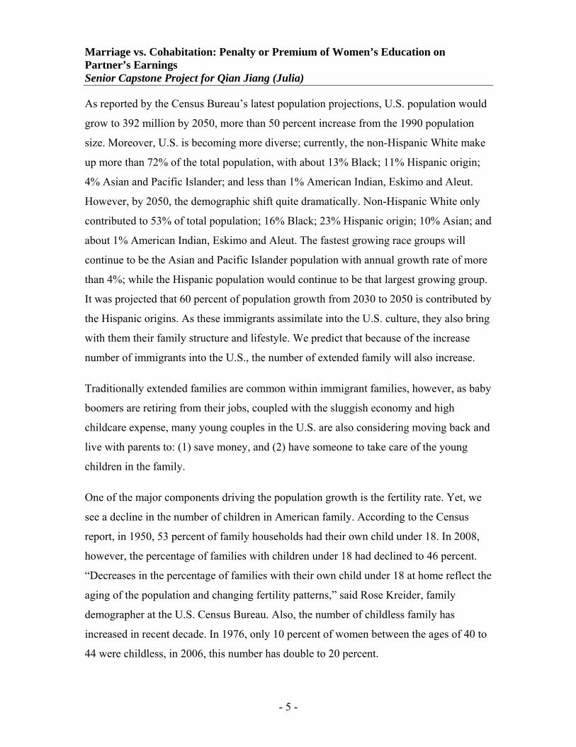
Furthermore, there is an increasing trend of deferring marriage age for both male and
female. We can see from Figure 1, the median age at first marriage in 1890 was relatively
high; during the 1950s, marriage age declined to its lowest level. However, since the
1970s there has been a consistent increase in first marriage age. In 2008, the median age
for men at first marriage was 27.4 years, and it was 25.6 years of age for women. Age at
marriage is an important indicator, because it makes the transition to adulthood in many
societies. Delayed age at marriage directly affects fertility by reducing the number of
years available for childbearing. Additionally, delayed marriage suggests that the society
is more urbanized, and a higher levels of educational attainment. Delayed marriage
allows women to attain higher education and gain labor force skills.
Figure 1: Median Age at First Marriage 1890 - 2008
Source:U.S. Bureau of the Census, 2003
In addition to deferring marriage age, less men and women in the U.S. are getting married.
In 2008, 66.9 million opposite six couples lived together, 60.1 million were married and
6.8 million were not. (Edwards, 2009) As the United States become increasingly diverse,
individuals of various backgrounds are introducing many new ideas, cohabitation before
marriage is one of the most complicated and controversial topics in the marriage area.
However, it has also become the norm in many countries. According to the U.S. Census
- 6 -
Marriage vs. Cohabitation: Penalty or Premium of Women’s Education on Partner’s Earnings Senior Capstone Project for Qian Jiang (Julia)
Bureau, approximately 90 percent of Americans will get married at some point in their
life, what has changed is that individuals are not waiting longer to marry but instead
many of them lived in cohabitation household.
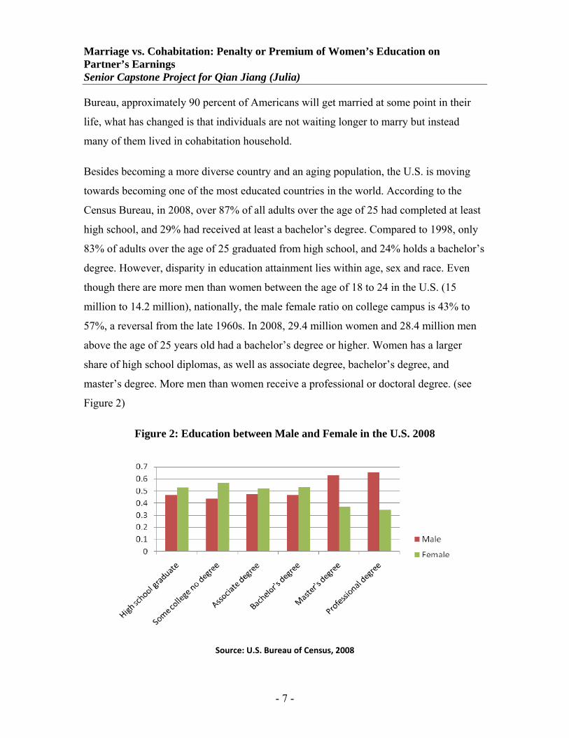
Besides becoming a more diverse country and an aging population, the U.S. is moving
towards becoming one of the most educated countries in the world. According to the
Census Bureau, in 2008, over 87% of all adults over the age of 25 had completed at least
high school, and 29% had received at least a bachelor’s degree. Compared to 1998, only
83% of adults over the age of 25 graduated from high school, and 24% holds a bachelor’s
degree. However, disparity in education attainment lies within age, sex and race. Even
though there are more men than women between the age of 18 to 24 in the U.S. (15
million to 14.2 million), nationally, the male female ratio on college campus is 43% to
57%, a reversal from the late 1960s. In 2008, 29.4 million women and 28.4 million men
above the age of 25 years old had a bachelor’s degree or higher. Women has a larger
share of high school diplomas, as well as associate degree, bachelor’s degree, and
master’s degree. More men than women receive a professional or doctoral degree. (see
Figure 2)
Figure 2: Education between Male and Female in the U.S. 2008
Source: U.S. Bureau of Census, 2008
- 7 -

Marriage vs. Cohabitation: Penalty or Premium of Women’s Education on Partner’s Earnings Senior Capstone Project for Qian Jiang (Julia)
- 8 -
According to the U.S. Census Bureau, among race, 53 percent of Asians in the U.S. had a
bachelor’s degree or more education. For non-Hispanic Whites it was 33 percent, 20
percent for blacks and 13 percent for Hispanics. Workers with a high school degree
earned an average of $31,286 in 2007, while those with a bachelor’s degree earned
$26,000 more on average ($57,181).
Women today accounts for 58% of all college undergraduates; 50% of law and medical
graduates, and 43% in business degrees. (Census Bureau, 2008) As more women are
becoming more marketable in the job market, labor force participation also increase in
the recent years. In 2008, women make up about 48% of the labor force and men 52 %,
compared to in 1948 women only account for 28% and men represent 72% of work force.
Lastly, as the U.S. becoming more technologically advance, many people now have the
freedom to work from home. As reported by the Current Population Survey, in may 2004,
20.7 million Americans work from home as part of their primary job, these workers
accounted from about 15 percent of total nonagricultural employment. Nearly two-thirds
of persons who usually worked at home were employed in management, professional,
and related occupations. One third of persons were self- employed. One in five sales
workers usually worked at home. Only three percent of workers in production and
transportation occupations. People employed in business services and education and
health services were most likely to work at home.
In 2004, 13.7 million wage and salary workers worked at home. About 3.3 million of
them had a formal arrangement with their employer. Of the 10.2 million workers who just
take work home from the job and without paid, 22 percent of them spend more than 8
hours per week at home. School teachers and instructors were especially likely to take
work home (Census, 2004).
The likelihood of working at home increased with educational attainment. Workers 25
years and over with a bachelor's degree or higher were 6 times more likely to work at
home as those without a high school diploma (32 and 5 percent, respectively). Much of
Marriage vs. Cohabitation: Penalty or Premium of Women’s Education on Partner’s Earnings Senior Capstone Project for Qian Jiang (Julia)
- 9 -
this disparity is due to the varying occupational patterns of workers with different levels
of education (Skatun, 2004).
Women and men have the same likelihood to be work at home in 2004, at about 15
percent each. Whites (16%) were twice as likely to work at home as blacks (8%) and
Hispanics (7%); 13% Asian worked at home in 2004. More parents with children tend to
work at home compared to persons without children. Married couples were more likely to
work at home than their non-married counterparts (Work At Home Summary, 2005).
Technological advances has made it possible for workers in many industries to work
from home. However, this form of work arrangement is not new, in fact, majority of
businesses were conducted this way before the Industrial Revolution. This enabled
businesses to control quantity of production, reduced costs, and provided work for
unskilled workers. (Boris, 1996)
According to the Canadian Survey of Work Arrangements (SWA), working from home is
more common in the service sector than in the goods industries. Most of these workers
are between the age of 25 and 54, professional and working in service industries.
Development of better communication information and technologies and the decrease of
cost of personal computer and other office equipments are two main factors that affect the
current trend of working from home.
Advantages for working from home are: reduction in expenses for work space, easier
recruitment and retention of staffs, increased the flexibility of workers, easier to reconcile
work and family responsibilities and reduced time of traveling. The disadvantages are:
communication problems with co-workers, hard to control efficiency of work; security
regarding information, fewer career possibilities, and possible increase in workload
(Perusse, 1998).
People often associate working from home with reduce in stress because better balancing
work and family life, however, the General Social Survey suggested that workers who
work from home have the same amount of stress as workers who work in a traditional

Marriage vs. Cohabitation: Penalty or Premium of Women’s Education on Partner’s Earnings Senior Capstone Project for Qian Jiang (Julia)
- 10 -
setting, regardless of their occupation or number of children (Fast and Grederick, 1996).
In addition, working from home does not necessarily reduce highway congestion or
transport-related pollution, because workers are making other kinds of trips to
compensate this (Pratte, 1996). However, working from home is not for everyone.
Studies suggested that working from home require a lot of disciplines from the workers,
therefore, only employees who are solitary, autonomous and qualified are suitable to
work from home (St-Onge and Lagasse, 1995). About 25% of workers who work at home
hold a university degree. Majority of these workers have more than one job. As of
November of 1995, 12% of employees who are working from home have working spouse,
8% are sole breadwinners, 7% live alone, and 10% are single parents (Perusse, 1998).
Working from home gives parents more flexibility to balance work and family, from
researches, we observed that most of these families have children under 16 years old.
Both Huws(1996) and Dooley(1996) argues that working from home is a solution to
balancing work and family, especially for women. Also, it gives access to people whose
childcare responsibility has restricted them from working in conventional environment.
Lastly, they agreed that this would increase household participant rate for male since
there is a less clear boundaries between work and home.
LITERATURE REVIEW Previous studies have analyze the effect of the wife’s education attainment on her
husband’s earnings, and across the board, we see a positive correlation in both developed
and developing countries.
According to Benhan (1974), formal education only provides an individual the ability to
acquire and assimilate information, and to understand and response to changing condition.
Close associate acts as a mediator that will further the educational development and this
close associate can influence the individual’s stock of knowledge. Spouse is arguably the
closest associate to an individual in his/her adulthood, thus spouse can assist a person’s
effective stock of education in three ways: First, spouse is a close substitute for formal
education, thus a highly educated wife can be better at giving sound advice and providing
Marriage vs. Cohabitation: Penalty or Premium of Women’s Education on Partner’s Earnings Senior Capstone Project for Qian Jiang (Julia)
- 11 -
information; Second, an educated wife can help her husband to acquire specific skills that
could lead to increase in productivity; Third, a well-informed wife can help her spouse to
acquire general skills related to information acquisition and assimilation thus better at
coping with changes. Moreover, individual’s effective stock of knowledge also depends
on the length of the association. Due to the low cost of sharing information between
couples than other kinships, couples generally have greater incentive to share acquired
abilities within the household, thus it is not difficult to see wife’s education improving
her husband’s earning capability by sharing information and suggestions on career
decisions. Agreeing with Benham, Wong (1986) concluded that wife’s education has a
significant effect on her husband’s earnings when the couple runs a family business
rather than working for an employer. Spouse can influence one’s consumption choices as
well as behavior in the labor market.
Loh(1996) also found that wife’s education attainment has a large positive impact on her
husband’s wage. This argument is found on the premise that wage and education
attainment have a positive correlation relationship. Also, Loh suggests that wife’s
education is a good proxy for potential wage. According to Skatun(2004), there is a
positive correlation between the wage of the worker and the potential wage of the spouse.
Therefore, we can conclude that education attainment of the worker is positively
correlated to the wage of their spouse.
Neuman and Ziderman (1990) found that in Israel, when a wife has at least a high school
education, the husband’s earnings are nine percent higher. A similar result found by
Scully (1979), in Iran, for each school year completed by wife, husbands earning raises
by four percent. In another study, Grossbard-Shechtman and Neuman (1991) found that
the wife’s years of schooling are positively associatedwith higher earnings for her
husband, and the size of the coefficient is about 3%. In Brazil, Lam and Schoeni (1994)
also found a positive effect, wife’s education accounts for 5% of husband’s earning in
1982, and 3-4% for the Unite States. Benham (1974) found that for each additional year
of schooling that wife complete, there is a 3-4% positive association with her husband’s
Marriage vs. Cohabitation: Penalty or Premium of Women’s Education on Partner’s Earnings Senior Capstone Project for Qian Jiang (Julia)
- 12 -
earnings. However, Astrom (2009) found that when husband has a high level of
education, there is a negative effect on the wife’s earnings unless she has a higher level of
education as well. Astrom believes that it takes a higher level of education to be able to
benefit from the productivity spillover effects from the partner. Differing from Astrom’s
finding, Huang (2009) found a positive association between the husband’s educational
level and the wife’s earning in China.
Besides reducing household earnings inequality (Amin, 2003), women’s education has
many other added benefits to their families, especially to their children. As reported by
Hill and King (1993), higher maternal educational level are positively associated with
improvements in children’s health, decrease infant mortality and better childhood
nutrition. Goldin (1992) found that woman with liberal arts education are more likely to
become a better wife, mother and homemaker, because a liberal arts education endowed
women the ability to use good judgment and reason to solve problems, thus better assist
her spouse in life. Also, having a spouse with a higher level of education is most likely to
associate with healthier behavior such as less smoking and less excessive drinking
(Monden, 2003). Individuals with higher education tend to be healthier; they are more
prone to engage in physical activities and preventive care (Groot and Maassen van den
Brink, 2007).
Using panel data from Malaysia, Jepsen (2005) suggested that government policies in
developing countries that help women to increase education could have positive effect for
families beyond the women’s own labor force participation and earnings. Jepsen also
observed that there is a decrease trend in the coefficient of women’s education to her
husband’s earnings. Jepsen believes this is caused by the increasing number of women
working thus spend more time outside of the family, less specialization in household
work. Thus, decrease the benefit of their education to their husband’s earnings. Also
better economic condition in recent years in Malaysia has increase husband’s
employment thus reduced the need for helps from their wives. Agreeing with Jepsen,
Song (2007) pointed out the concept of working spouse penalty/premium. According to
Marriage vs. Cohabitation: Penalty or Premium of Women’s Education on Partner’s Earnings Senior Capstone Project for Qian Jiang (Julia)
- 13 -
Song, working spouse penalty arise when working wife’s work hour increase. Because
longer hours devoted to work means less division of labor within the household, married
men whose wives are working earn lower wages than do comparable men with non-
working wives. However, Song stated that working wife is only associated with lowering
husband’s wage if he is in the management position, but will increase husband’s wage
among non-managers. Lastly, Song argued that it is not husband’s occupation that
triggers the working spouse penalty or premium rather the distribution of husband’s wage
level.
Although labor economists might not agree on the magnitude and the cause of marriage
wage premium, most of them would accept that marriage has a positive wage effect for
male workers.
One of the dominant theories is the productivity hypothesis, which argues that marriage
makes men more productive (Becker, 1991) (Chun and Lee, 2001). This argument is
found on the premise of household specialization. It assumes that if the wife of a married
man performs most of the work in the household, it will increase the opportunity for the
married man to specialize in the labor market thus be more productive and have higher
earnings. Single men have lower productivity because they have to perform additional
work in the household, thus are not fully committed to the labor market. According to
Chun and Lee (2001) and Jepsen (2005), men whose wives specialize in home production
have a larger premium than men whose wives work in the labor market. Moreover, the
gains from marriage are positively associated with the degree of specialization within the
household. For every additional hour a wife work in the labor market, per week, wage
gain from marriage decreased by 0.6%.
A competing argument to the productivity hypothesis is the selection hypothesis
proposed by Nakostenn and Zimmers (1987, 1997, 2001). This theory states that
selection of marriage is not always solely base on emotional factors; there are other
factors that determine whether a man finds a mate, such as having an attractive physique,
a high intelligence and a stable economic basis. Although, physical appearance and IQ

Marriage vs. Cohabitation: Penalty or Premium of Women’s Education on Partner’s Earnings Senior Capstone Project for Qian Jiang (Julia)
- 14 -
are individual traits that cannot be record or are hard to gather by researchers, they are
have been study and proven to be positively related to earnings potential. According to
Hamermesh and Biddle (1994), physical appearance has a significant impact on earnings;
people with plain-featured earn less than people with average looks, who earn less than
people who are attractive. Therefore, men with higher earnings ability become more
attractive in the marriage market, ceteris paribus, consequently they are more likely to get
married. Married men are more productive before they were married, their productivity
enable them to have higher earnings; not because they become more productive after
marriage, there is no marriage premium exist. In line with Becker’s assortative mating
theory, people tend to marry to a partner with similar traits with respect to age, education,
wealth, religion, and race.
Thus, highly educated individuals tend to marry other highly educated individuals, and
high wage earners tend to marry each other. As stated in Schwartz and Mare (2005),
Americans are becoming more educationally homogamous; often time they are paired off
by education level. A high school graduate marrying someone with a college degree
declined by 43 percent from 1940 to the late 1970s. Nevertheless, the evidence is mixed.
Chun and Lee (2001) found that there is little evidence to support the selection hypothesis.
Unmeasured earning capabilities are not positively correlated with unobservable traits
valued in the marriage selection process.
Skatun (2004) proposed that individual in a collective partnership have a better
bargaining position than a single individual. Skatun pointed out that the difference in
wage earning in married and non married men might be due to their bargaining power in
the labor market. In the labor market, if a married man failed to reach an agreement with
his employer, he still has a safety net, which he can always relied on, and fall back on a
share of their partner’s income. This hypothesis argues that worker in a collective
relationship are generally less impatient, thus they are less likely to enter into an
agreement with the firm when their partner’s income is high, as he/ she is not in need of
money. Therefore, married men have a lower threat point than single men, and they can

Marriage vs. Cohabitation: Penalty or Premium of Women’s Education on Partner’s Earnings Senior Capstone Project for Qian Jiang (Julia)
- 15 -
extract a higher compensation from the firm. Skatun also suggests that married workers
would use their partner’s wage as leverage in the bargaining process. Furthermore,
primary workers tend to do better than secondary workers, which explain why men earn
more than women. As pointed out by Lundberg and Rose (2000), as a mother’s wage and
hour worked falls, father’s wages and hours worked increase. Worker’s wage is generally
higher if 1) the partner’s current income is lower and 2) if the partner’s potential income
is high.
Some researchers suggested that the differences between married and single men
earnings may be caused by sociological reasons. There are no actual difference in
productivity between married men and single men. Pfeffer and Ross(1982) 1 argued that
married men are paid more because employers reward them for conforming to social
conventions. The conformance argument is that men have a social expectation to be
married and support their families; working women on the other hand, should work only
because of divorce or being widowed. Therefore, when men are married and working,
they are conforming to social expectations, but when women are married and working,
they are not. This also explains the differential effect of marital status on men and women
workers.
Another reason for the marriage premium exists in male workers is the argument of
compensating differentials. This argument is relatively similar to the conformance
argument in which suggest that married men are expected to provide for the family,
therefore, they seek money rather than non-wage compensation (Reed and Harford, 1988).
Since there are no information on productivity alone, most of the previous studies use the
presence of certain wages patterns to support the productivity argument. Kenny(1983)
and Neumark (1991) found that wage rates rise faster during marriage, Hill (1979)
reported that married men spend more time in training on current jobs than non married
men. Lynch (1992) and Sicherman (1993) both found that married men and women are
more likely to have receive company or on the job trainings.
1 As referenced in Skatun( 2004)

Marriage vs. Cohabitation: Penalty or Premium of Women’s Education on Partner’s Earnings Senior Capstone Project for Qian Jiang (Julia)
- 16 -
Studies of changes in family household structures in the United States have noted a
downward trend during most of the 20th century in the prevalence of extended family
households (Goldscheider, 1989), however during the 1980s, the decline in extended
family have slow down. Households that contain extended family members increased
from 10 percent in 1980 to 12 percent in 1990 (Glick, Bean, VanHook, 1997). One factor
is immigration. During the 1970s and 1980s, United States undertake a dramatic shift in
both the volume and composition of immigrants. Majority of these immigrants are now
coming from less developed countries where extended family structures are more
common, 83% of total immigrants are from Asia and Latin America (U.S. Immigration
and Naturalization service, 1995).
Migrants from Mexico and other Central American countries are more likely to come to
the United States as labor migrants, thus are more likely to utilize social networks of
distant relatives for housing, employment and other assistance (Glick, et al. 1997). These
labor migrants are more likely to share households with horizontal extended relative such
as siblings or cousins rather than grandparents (Chavez, 1985). On the other hand, during
the 1980s, many immigrants entered into the U.S. as refugees, they came with multiple
generation family members and have little hope of returning to their country of origin,
thus are more likely to form vertically extended households (Chavez, 1990).
Family researchers study kinship support by focus on three key types: emotional,
financial, and instrumental (such as physical and practical supports). Childcare help is an
independent type of support as it has both instrumental and emotional components
(Sarkisian et al. 2006).
Studies have found that Latinos were more likely than Whites to live with extended kin
(Sarkisian, et al. 2006). Furthermore, comparing Latino groups with each others, we see
that Mexicans were more likely to co-reside with extended kin than Puerto Ricans and
other Latinos (De Vos and Arias, 2003). Moreover, researchers have found that Latinos
are less likely to give financial assistance and more likely to provide instrumental helps
and childcare help. Higher socioeconomic status was associated with less co-residence
Marriage vs. Cohabitation: Penalty or Premium of Women’s Education on Partner’s Earnings Senior Capstone Project for Qian Jiang (Julia)
- 17 -
and with a greater likelihood of giving financial support. Furthermore, according to
Sarkisian, Gerena and Gerstel, (2006), having a partner or minor children decreased the
likelihood of co-residence, but increased the likelihood of living near kin. Single parent
increased the likelihood of giving instrumental help, and being a nonresident parent
increased the likelihood of giving financial assistance.
DATA AND SUMMARY STATISTICS This paper is conducted using the U.S. Census’ Current Population Survey (CPS) data for
the years of 1979 and 2009. The CPS sample consists of 154,452 observations for 1979
and 207,921 observations for 2009. These data contain the information needed to
compare the characteristics and earnings abilities of individuals. However, when we
restrict our sample to those couples with all of the necessary socio-economic information,
we are left with 131,216 observations for 1979 and 91,145 observations for 2009. The
dependant variable is the log of the husband and partner’s annual earnings. The data are
restricted to husbands and partners who work full time, where full time is defined as
working at least 35 hours per week and at least 45 weeks per year. We follow Benham
(1974) and define potential work experience as age minus schooling minus six.
Education attainment is a category variable defined by CPS. We group the CPS
categories in to seven education levels: have 12th grade or less education, High school
graduate or GED holder, Associate degree or have some years of college education, holds
Bachelor’s degree, holds Master degree, and holds Doctorate degree. Data are
representing the highest level of formal school that the individual has completed.
The empirical model also includes variables such as race and location of residence to
avoid the risk of omitted variable Race variable is measured as a series of dummy
variables includes white, black, Asian, and Hispanic. Asian is the additional race added to
this study that previous studies had neglected. It is estimated by the Census that by 2050,
10% of U.S. population would be Asian descents. We feel that it is important to include
this race in the analysis. Metropolitan level is a location variable. Based on the

Marriage vs. Cohabitation: Penalty or Premium of Women’s Education on Partner’s Earnings Senior Capstone Project for Qian Jiang (Julia)
- 18 -
household’s location, we categorized all sample data into two groups: rural and urban.
We presumably believe that urban workers earn more than workers from rural area.
Educated wife would have a bigger influence to her family’s stand of living if she works
in the urban area.
Because of lack of availability of data, we will use the number of married couples in a
household (NCOUPLES) as proxy for extended family. If the number of couples in
household in family is equal to 0, then we can say people who live in this household are
in a cohabitating relationship. If the number of couples in household is more than 1, then
we say there are extended family members living in the household. Moreover, we use
number of children between 13-30 in the household as another proxy variable to reflect
extended family. We believed older children in the family can help out parents to raise
younger siblings, therefore act as a second set of parents. This study uses the number of
home based business and self employed workers as proxies for working from home.
To implement our model, we need to have information on wife’s individual characteristic
as well as other family characteristic such as number of children in the household and the
metropolitan level of reside city. However, the CPS data are constructed in a way that
multiple families or unrelated persons are sometimes included in the same household.
Therefore, matching husband with his exact wife is critical to the process. We used
household serial number and relation identification information to match couples so that
we can draw conclusion on how wife’s education affects her spouse’s earnings.
Table 1 presents the summary of statistics of the male sample by marital status. All
participant males are categorized into three categories: Married (spouse present), Married
but lived alone (spouse absent), and never been married. Married with absent spouse are
men who are divorce, separated from their spouse, widower or spouse working away
from home. Reasons to have a separate category is because we presume married men
earn more because of their spouse/partner helps them to be more productive by sharing
household chores. On the contrary, married men who live alone do not necessarily enjoy
the same marriage premium those married men who do live with spouse. Therefore, by
Marriage vs. Cohabitation: Penalty or Premium of Women’s Education on Partner’s Earnings Senior Capstone Project for Qian Jiang (Julia)
- 19 -
having a separate category we are able to observe whether there is any difference
between married men with spouse present and married men with absent spouse.
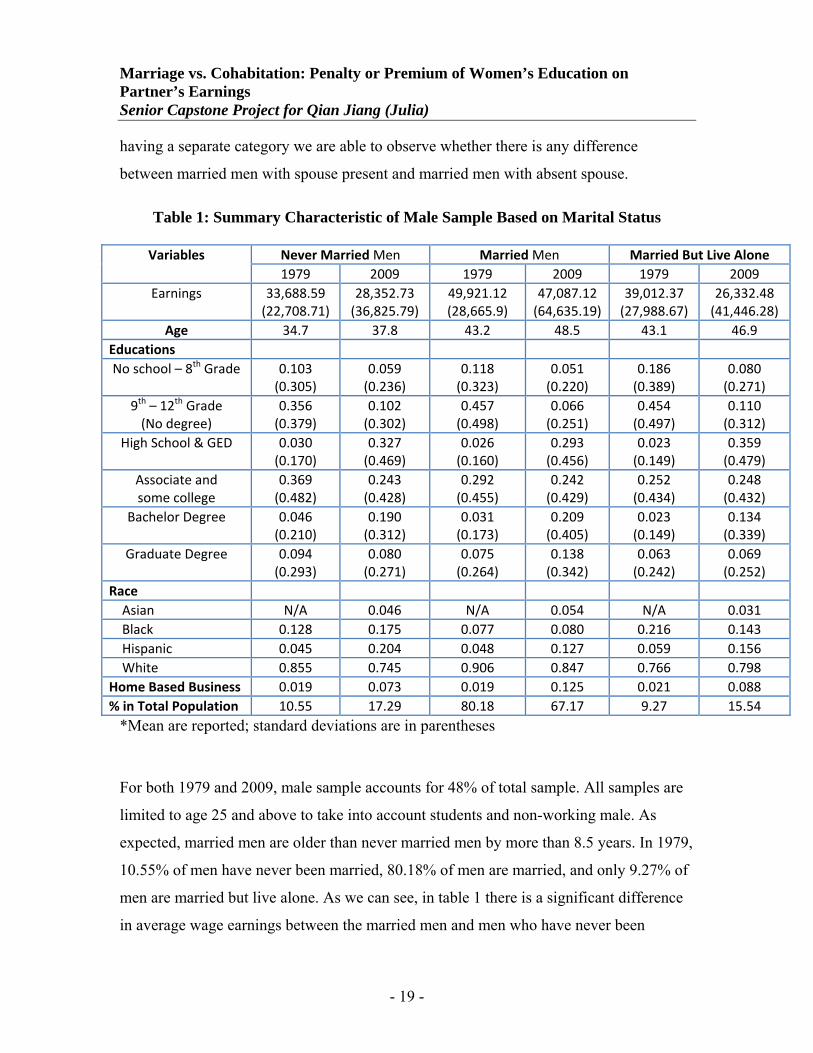
Table 1: Summary Characteristic of Male Sample Based on Marital Status
Variables Never Married Men Married Men Married But Live Alone 1979 2009 1979 2009 1979 2009
Earnings 33,688.59 (22,708.71)
28,352.73 (36,825.79)
49,921.12 (28,665.9)
47,087.12 (64,635.19)
39,012.37 (27,988.67)
26,332.48 (41,446.28)
Age 34.7 37.8 43.2 48.5 43.1 46.9 Educations No school – 8th Grade 0.103
(0.305) 0.059 (0.236)
0.118 (0.323)
0.051 (0.220)
0.186 (0.389)
0.080 (0.271)
9th – 12th Grade (No degree)
0.356 (0.379)
0.102 (0.302)
0.457 (0.498)
0.066 (0.251)
0.454 (0.497)
0.110 (0.312)
High School & GED 0.030 (0.170)
0.327 (0.469)
0.026 (0.160)
0.293 (0.456)
0.023 (0.149)
0.359 (0.479)
Associate and some college
0.369 (0.482)
0.243 (0.428)
0.292 (0.455)
0.242 (0.429)
0.252 (0.434)
0.248 (0.432)
Bachelor Degree 0.046 (0.210)
0.190 (0.312)
0.031 (0.173)
0.209 (0.405)
0.023 (0.149)
0.134 (0.339)
Graduate Degree 0.094 (0.293)
0.080 (0.271)
0.075 (0.264)
0.138 (0.342)
0.063 (0.242)
0.069 (0.252)
Race Asian N/A 0.046 N/A 0.054 N/A 0.031 Black 0.128 0.175 0.077 0.080 0.216 0.143 Hispanic 0.045 0.204 0.048 0.127 0.059 0.156 White 0.855 0.745 0.906 0.847 0.766 0.798 Home Based Business 0.019 0.073 0.019 0.125 0.021 0.088 % in Total Population 10.55 17.29 80.18 67.17 9.27 15.54
*Mean are reported; standard deviations are in parentheses
For both 1979 and 2009, male sample accounts for 48% of total sample. All samples are
limited to age 25 and above to take into account students and non-working male. As
expected, married men are older than never married men by more than 8.5 years. In 1979,
10.55% of men have never been married, 80.18% of men are married, and only 9.27% of
men are married but live alone. As we can see, in table 1 there is a significant difference
in average wage earnings between the married men and men who have never been

Marriage vs. Cohabitation: Penalty or Premium of Women’s Education on Partner’s Earnings Senior Capstone Project for Qian Jiang (Julia)
- 20 -
married. The average earnings of married men is 32.5% higher than that of never married
men. On average, married men earn $16,232 more per year than their non married
counterparts. Men whose spouse is absent earns 13.6% more than men who have never
been married, but earns 27.9% less than married men with spouse present. This income
gap between married men and never married man confirms the marriage premium theory
while the income gap between married men who live with spouse and married men with
absent spouse verifies the productivity theory.
If we accept the Selection theory or the Assortative mating theory, we would think that
married men would have a higher education than never married men. Because one of the
basis for these two theories is that married men were productive before they get marriage,
marriage did not make them more productive. And because productive men generally
have higher earning power therefore, they are more likely to attract mates. However, our
results tell us differently. In 1979, never married men actually have the highest education
within the three groups. 36.9% of these men have an associate degree, 4.6% holds a
bachelor degree, and 9.4% received a doctoral degree. While only 29.2%, 3.1%, 7.5% of
married men have the same degree and 25.2%, 2.3%, 6.3% for married men with absent
spouse. This could be the explanation of why never married men on average have higher
education then married men; because most of the single men are still in school pursuing
education. Lastly, White male appeared to be more likely to be married than Asian, Black
and Hispanic male.
In 2009, number of never married men increased 6.74 percentage points from 1979 to
2009’s 17.29%; at the same time, number of married men drop from 80.18% to 7.17%;
married but living alone rise to 15.54%. The results not only verify the current trend of
delaying marriage but also suggest that more divorce have occurred compared to thirty
years ago.
As expected, married men still have the highest earnings, roughly 39.7% higher than men
who have never been married and 44% more than married men with absent spouse.
Despite adjusting for inflation, all three groups of men earn less than what it would be in

Marriage vs. Cohabitation: Penalty or Premium of Women’s Education on Partner’s Earnings Senior Capstone Project for Qian Jiang (Julia)
- 21 -
1979. Earnings for never married men decreased by 18.8%; 1.5% for married men and
48% decline for married men with absent spouse.
Education attainment for men has increased significantly compare to what it was in 1979.
Lesser people have 12th grade or less education; 84% of men in 2009 have at least
complete high school or have a GED compare to only 53.9% in 1979. Unlike 1979, there
is a mixed result for the educational attainment for the three marital groups, there is
dominant group being the most educated. However, in 2009, married men accounts for
the most in high education. 20.9% of married men have bachelor degree and 13.8%
graduate degree; 19% of never married men graduated from college, and 8% went to
graduate school.
In 2009, White male still have an advantage over other male at marriage; however, Black
and Hispanic male has reversed role. In 1979, Black men are have the most disadvantage
when it comes to marriage, but today, Hispanic male replaced Black male and become
the most unlikely to get married. Number of home based worker has also increased
substantially, In 2009, 28.6% of all men work from home compare to 1979 only 5.9%.
Marriage vs. Cohabitation: Penalty or Premium of Women’s Education on Partner’s Earnings Senior Capstone Project for Qian Jiang (Julia)
- 22 -
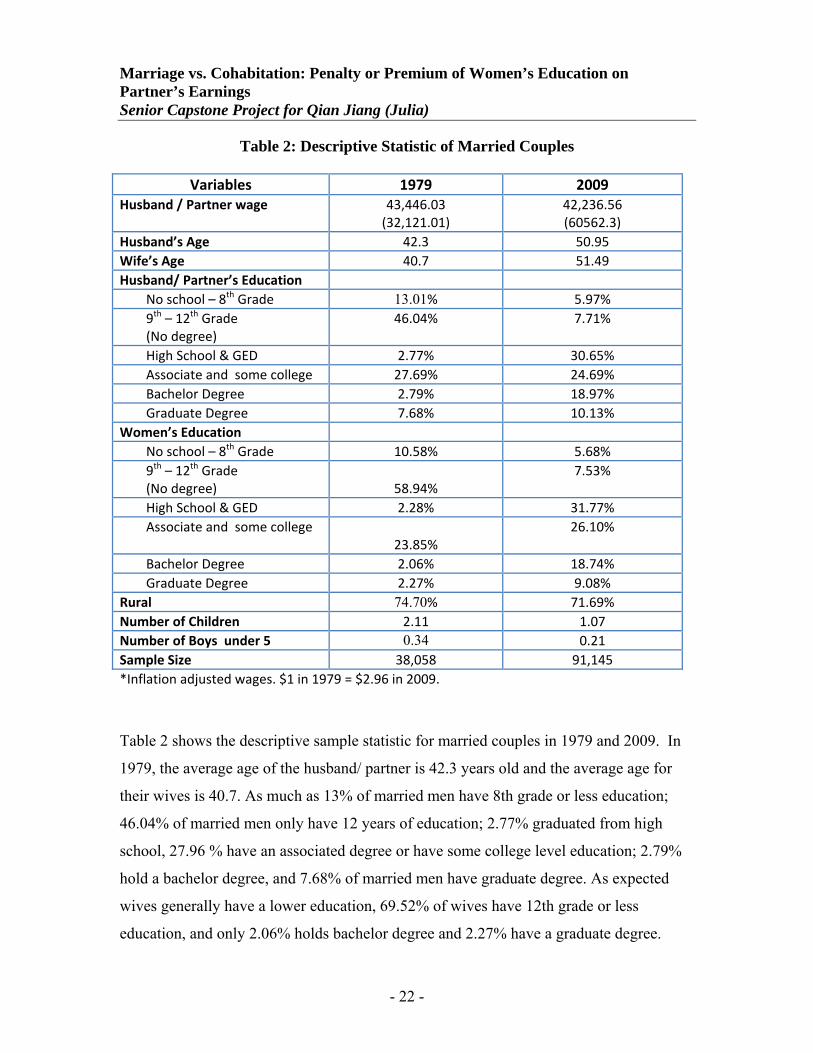
Table 2: Descriptive Statistic of Married Couples
Variables 1979 2009 Husband / Partner wage 43,446.03
(32,121.01) 42,236.56 (60562.3)
Husband’s Age 42.3 50.95 Wife’s Age 40.7 51.49 Husband/ Partner’s Education No school – 8th Grade 13.01% 5.97% 9th – 12th Grade (No degree)
46.04% 7.71%
High School & GED 2.77% 30.65% Associate and some college 27.69% 24.69% Bachelor Degree 2.79% 18.97% Graduate Degree 7.68% 10.13% Women’s Education No school – 8th Grade 10.58% 5.68% 9th – 12th Grade (No degree)
58.94%
7.53%
High School & GED 2.28% 31.77% Associate and some college
23.85% 26.10%
Bachelor Degree 2.06% 18.74% Graduate Degree 2.27% 9.08% Rural 74.70% 71.69% Number of Children 2.11 1.07 Number of Boys under 5 0.34 0.21 Sample Size 38,058 91,145 *Inflation adjusted wages. $1 in 1979 = $2.96 in 2009.
Table 2 shows the descriptive sample statistic for married couples in 1979 and 2009. In
1979, the average age of the husband/ partner is 42.3 years old and the average age for
their wives is 40.7. As much as 13% of married men have 8th grade or less education;
46.04% of married men only have 12 years of education; 2.77% graduated from high
school, 27.96 % have an associated degree or have some college level education; 2.79%
hold a bachelor degree, and 7.68% of married men have graduate degree. As expected
wives generally have a lower education, 69.52% of wives have 12th grade or less
education, and only 2.06% holds bachelor degree and 2.27% have a graduate degree.
Marriage vs. Cohabitation: Penalty or Premium of Women’s Education on Partner’s Earnings Senior Capstone Project for Qian Jiang (Julia)
- 23 -
However, women have similar percentage in Associate degree as men, both around 24%.
In 1979, roughly 25% of the couples live in urban area, which suggests a disparity
between urban and rural residents in the sample. Average couple has 2.11 children in the
household, and one out of three families have children under the age of 5. Table 3 shows
the number of couples in household which suggests the presence of extended families and
percentage of cohabitation within population about 0.99% of all households has more
than one family living together. 11.15% of couples live together but are not married.
2.32% of families have more than one mother in the household, 0.84% of families have
more than one father in the household. These results indicates the existence of
grandparents.
In 2009 both age and education attainment increased significantly for both sexes. Only
13.68% of married men have less than 12th years of education compare to 46.04% in
1979. 30.65% graduated from high school or have a GED; 24.69% have an associate
degree or have some years of college level education; 18.97% have a bachelor degree;
12.02% have a graduate degree. Education increased even more dramatically for women,
in 2009, only 13.21% of all married women have less than 12 years education, this is
almost a 80% decreased in the number of women who have less than 12th grade
education from 1979. Also, for the first time women has less percentage than men in the
lower education level. As of 2009, the numbers of women who have higher education are
almost the same as the number of men who have higher education. 18.74% of married
women now have a bachelor degree, 10.18% has graduate degree. This significant
increased in the number of married women in higher education is not too surprising given
the fact that American women are more educated than women in other parts of the world;
also, women have tried very hard to gain equality in the recent decades.
In 2009, the average age of the husbands is 50.95, which is 8.65 years older than the
average age in 1979. Disparity between urban family and rural family are still wide more
couples move out of urban city and choose to live in rural area, 28.31% couples are from
urban area. Couples are now considering to have less children in the family, on average
Marriage vs. Cohabitation: Penalty or Premium of Women’s Education on Partner’s Earnings Senior Capstone Project for Qian Jiang (Julia)
- 24 -
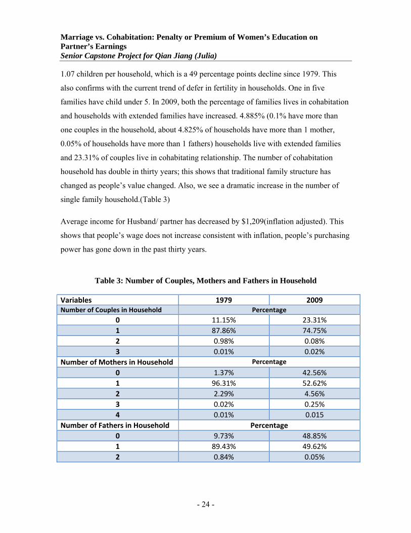
1.07 children per household, which is a 49 percentage points decline since 1979. This
also confirms with the current trend of defer in fertility in households. One in five
families have child under 5. In 2009, both the percentage of families lives in cohabitation
and households with extended families have increased. 4.885% (0.1% have more than
one couples in the household, about 4.825% of households have more than 1 mother,
0.05% of households have more than 1 fathers) households live with extended families
and 23.31% of couples live in cohabitating relationship. The number of cohabitation
household has double in thirty years; this shows that traditional family structure has
changed as people’s value changed. Also, we see a dramatic increase in the number of
single family household.(Table 3)
Average income for Husband/ partner has decreased by $1,209(inflation adjusted). This
shows that people’s wage does not increase consistent with inflation, people’s purchasing
power has gone down in the past thirty years.
Table 3: Number of Couples, Mothers and Fathers in Household
Variables 1979 2009 Number of Couples in Household Percentage
0 11.15% 23.31% 1 87.86% 74.75% 2 0.98% 0.08% 3 0.01% 0.02%
Number of Mothers in Household Percentage
0 1.37% 42.56% 1 96.31% 52.62% 2 2.29% 4.56% 3 0.02% 0.25% 4 0.01% 0.015
Number of Fathers in Household Percentage 0 9.73% 48.85% 1 89.43% 49.62% 2 0.84% 0.05%
Marriage vs. Cohabitation: Penalty or Premium of Women’s Education on Partner’s Earnings Senior Capstone Project for Qian Jiang (Julia)
- 25 -
METHODOLOGY In order to analyze the different questions posed in this paper, more than one model is
used. The baseline model is based on the modified version of Jepsen’s model which was
a modified version of Mincer (1974) and Benham (1974)’s ordinary least squares (OLS)
wage model.
To answer how women’s education is affecting her spouse/partner’s earnings, we use
equation one. Our model adds four important independent variables, including Asian race,
number of children in household, homebased worker, and extended family.
Incwage Husband = β0 + β1Educmen + β2Educwife + β3Age + β4Exp + β5Exp2 + β6Race + β7Metro + β8Marst + β9Nchild5 + β10Child13 + β11Ncouples + β12Homebased + ε
(1) Where, Incwage is the natural log of income of husband’s annual earnings; Educ is a
vector of variables of male and female individual; Exp is work experience which is
defined as
Age – Schooling – 6; Race includes Asian, Black, Hispanic, and White; Metro level
indicates whether the individual is living in a urban city or not; Nchild5 is the number of
children under the age of 5 in a household; Child13 is number of children between 13 to
30 in a household; Ncouples is the number of couples in household.
We will estimate the model twice by changing the dependent variable. Particularly, we
change spouse’s earning to partner’s earnings. Then we will compare the results and
conclude whether men in a cohabitating relationship are impacted the same way (or not)
as married men when their wives increase education attainment.
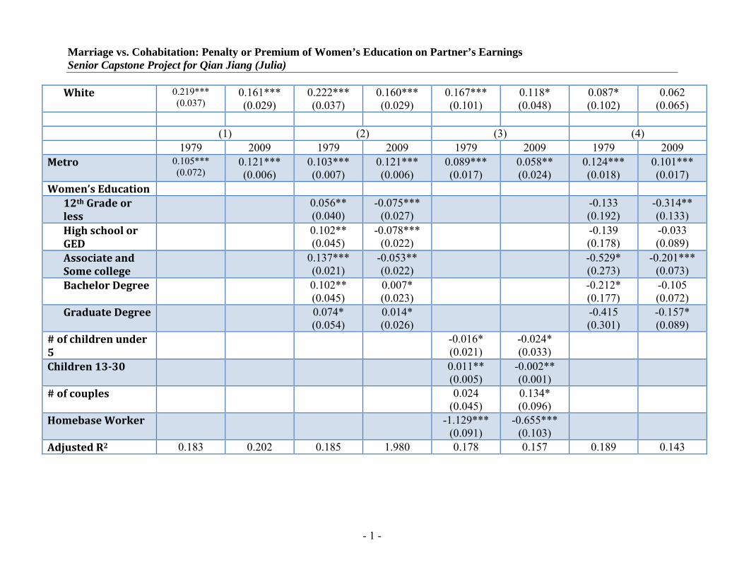
EMPIRICAL RESULTS Regression (1) of table 4 is a basic regression of Men’s annual earning with dependent
variable being husband’s earnings. This regression acts as a baseline for the future
Marriage vs. Cohabitation: Penalty or Premium of Women’s Education on Partner’s Earnings Senior Capstone Project for Qian Jiang (Julia)
- 26 -
comparisons. We see from table 4 that a man’s own education attainment and experience
are significant predictors of his earnings, as a man’s education level increase his earnings
increase, work experience shows a positive correlation at 10% significant level. Return to
each level of education is larger in 2009 than in 1979. In 1979, only when education
attainment is 12th grade or less there is a negative impact on earnings, all other levels
have positively effects. However, compare to Associate and Bachelor degree, graduate
degree has relatively smaller effect. In 2009, any education level less than Bachelor
degree have negative impact on earnings, this is suggesting that in today’s society,
education is more important than what it was in the late 70’s in obtaining a job. Compare
to minority, White male has advantage when it comes to earnings, which is in line with
previous studies. However, the degree of the negative impact increased in 2009 for Black
and Hispanic males while the positive effect for White male has shrunk. Metropolitan
level shows the individual’s current reside city, as expected, people who live in the
urban/central city make more than people who live in the rural part of the country. Result
is same for both years, with very minor changes.
Regression (2) examine the effect of women’s educational attainment has on husband’s
earnings. The coefficient of different levels of education for women differs significantly
between the two years. In 1979, all levels of educational attainment for women would
have positive effect on husband’s earnings. This is not surprising since majority of
women in the late 70’s does not have a high education, therefore, any level of education
is sufficient. The largest positive effect for having an Associate degree shows that people
view that as a practical degree and the relative smaller positive effects in the Graduate

Table Variables (1) (2) (3) (4)
1979 2009 1979 2009 1979 2009 1979 2009 Constant 8.533***
(0.079) 9.521*** (0.174)
8.533*** (0.069)
9.173*** (0.083)
8.832*** (0.109)
8.198*** (0.507)
7.823*** (0.296)
9.745*** (0.467)
Men Age 0.060*** (0.003)
0.014*** (0.005)
0.062*** (0.003)
0.014** (0.005)
0.060*** (0.005)
0.053* (0.028)
0.083*** (0.011)
0.019* (0.018)
Men Experience 0.006** (0.004)
0.032* (0.005)
0.008* (0.004)
0.033*** (0.005)
0.015** (0.006)
0.013 (0.053)
0.022* (0.012)
0.025* (0.019)
Men’s Experience2 -0.001** (0.001)
-0.001*** (0.001)
-0.001*** (0.001)
-0.001*** (0.001)
-0.001*** (0.005)
-0.001 (0.002)
-0.001*** (0.001)
-0.001*** (0.001)
Men Education 12th Grade or less
-0.008* (0.031)
-0.940*** (0.050)
0.013*** (0.019)
-0.232*** (0.053)
-0.019* (0.031)
-0.993*** (0.246)
0.264* (0.023)
-0.398 (0.282)
High school or GED
0.016* (0.032)
-0.698*** (0.035)
0.033* (0.019)
0.241*** (0.027)
0.005* (0.046)
0.527*** (0.081)
0.197* (0.188)
-0.759*** (0.173)
Associate and Some college
0.061*** (0.018)
-0.555*** (0.030)
0.076*** (0.019)
0.367*** (0.031)
0.036* (0.045)
0.702*** (0.099)
0.655** (0.278)
-0.383*** (0.146)
Bachelor Degree 0.159*** (0.037)
0.698*** (0.038)
0.116** (0.038)
0.648*** (0.041)
0.121** (0.059)
0.974*** (0.163)
0.269* (0.177)
-0.346*** (0.126)
Graduate Degree 0.049* (0.01)
0.939*** (0.050)
0.500* (0.031)
0.882*** (0.052)
0.032* (0.062)
0.993*** (0.246)
0.430 (0.298)
0.038 (0.105)
Race Asian N/A 0.023*
(0.036) N/A 0.020
(0.036) N/A 0.094*
(0.134) N/A -0.065
(0.095) Black -0.035*
(0.041) -0.090** (0.033)
-0.036* (0.042)
-0.090** (0.033)
-0.063* (0.112)
-0.101* (0.120)
-0.202** (0.108)
-0.034 (0.072)
Hispanic -0.157*** (0.020)
-0.180*** (0.016)
-0.149*** (0.020)
-0.177*** (0.016)
-0.051** (0.047)
-0.060* (0.048)
-0.107** (0.054)
-0.175*** (0.041)
Marriage vs. Cohabitation: Penalty or Premium of Women’s Education on Partner’s Earnings Senior Capstone Project for Qian Jiang (Julia)
- 1 -
White 0.219*** (0.037)
0.161*** (0.029)
0.222*** (0.037)
0.160*** (0.029)
0.167*** (0.101)
0.118* (0.048)
0.087* (0.102)
0.062 (0.065)
(1) (2) (3) (4) 1979 2009 1979 2009 1979 2009 1979 2009
Metro 0.105*** (0.072)
0.121*** (0.006)
0.103*** (0.007)
0.121*** (0.006)
0.089*** (0.017)
0.058** (0.024)
0.124*** (0.018)
0.101*** (0.017)
Women’s Education 12th Grade or less
0.056** (0.040)
-0.075*** (0.027)
-0.133 (0.192)
-0.314** (0.133)
High school or GED
0.102** (0.045)
-0.078*** (0.022)
-0.139 (0.178)
-0.033 (0.089)
Associate and Some college
0.137*** (0.021)
-0.053** (0.022)
-0.529* (0.273)
-0.201*** (0.073)
Bachelor Degree 0.102** (0.045)
0.007* (0.023)
-0.212* (0.177)
-0.105 (0.072)
Graduate Degree 0.074* (0.054)
0.014* (0.026)
-0.415 (0.301)
-0.157* (0.089)
# of children under 5
-0.016* (0.021)
-0.024* (0.033)
Children 1330 0.011** (0.005)
-0.002** (0.001)
# of couples 0.024 (0.045)
0.134* (0.096)
Homebase Worker -1.129*** (0.091)
-0.655*** (0.103)
Adjusted R2 0.183 0.202 0.185 1.980 0.178 0.157 0.189 0.143
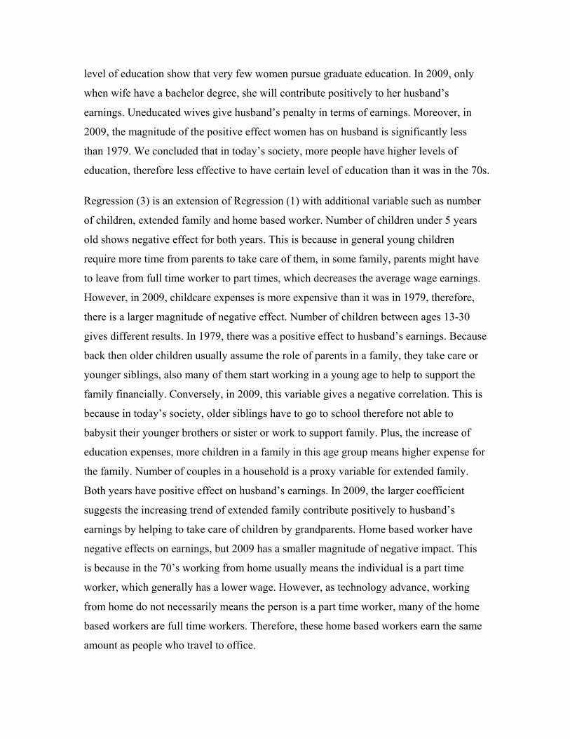
level of education show that very few women pursue graduate education. In 2009, only
when wife have a bachelor degree, she will contribute positively to her husband’s
earnings. Uneducated wives give husband’s penalty in terms of earnings. Moreover, in
2009, the magnitude of the positive effect women has on husband is significantly less
than 1979. We concluded that in today’s society, more people have higher levels of
education, therefore less effective to have certain level of education than it was in the 70s.
Regression (3) is an extension of Regression (1) with additional variable such as number
of children, extended family and home based worker. Number of children under 5 years
old shows negative effect for both years. This is because in general young children
require more time from parents to take care of them, in some family, parents might have
to leave from full time worker to part times, which decreases the average wage earnings.
However, in 2009, childcare expenses is more expensive than it was in 1979, therefore,
there is a larger magnitude of negative effect. Number of children between ages 13-30
gives different results. In 1979, there was a positive effect to husband’s earnings. Because
back then older children usually assume the role of parents in a family, they take care or
younger siblings, also many of them start working in a young age to help to support the
family financially. Conversely, in 2009, this variable gives a negative correlation. This is
because in today’s society, older siblings have to go to school therefore not able to
babysit their younger brothers or sister or work to support family. Plus, the increase of
education expenses, more children in a family in this age group means higher expense for
the family. Number of couples in a household is a proxy variable for extended family.
Both years have positive effect on husband’s earnings. In 2009, the larger coefficient
suggests the increasing trend of extended family contribute positively to husband’s
earnings by helping to take care of children by grandparents. Home based worker have
negative effects on earnings, but 2009 has a smaller magnitude of negative impact. This
is because in the 70’s working from home usually means the individual is a part time
worker, which generally has a lower wage. However, as technology advance, working
from home do not necessarily means the person is a part time worker, many of the home
based workers are full time workers. Therefore, these home based workers earn the same
amount as people who travel to office.
Marriage vs. Cohabitation: Penalty or Premium of Women’s Education on Partner’s Earnings Senior Capstone Project for Qian Jiang (Julia)
- 1 -
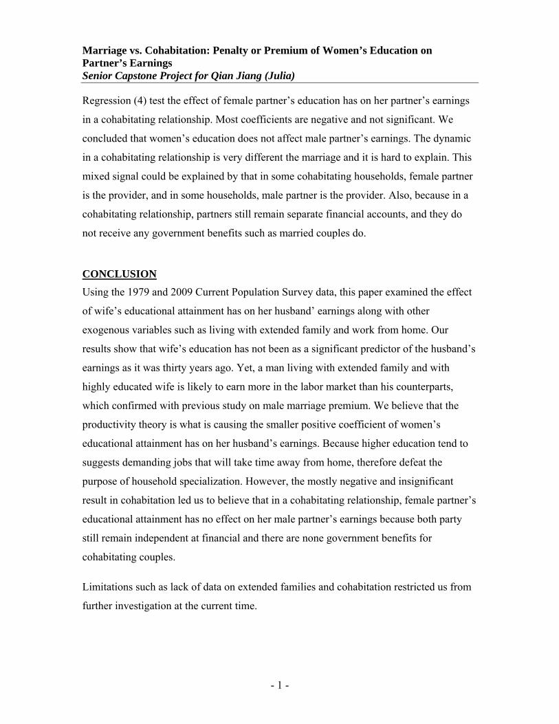
Regression (4) test the effect of female partner’s education has on her partner’s earnings
in a cohabitating relationship. Most coefficients are negative and not significant. We
concluded that women’s education does not affect male partner’s earnings. The dynamic
in a cohabitating relationship is very different the marriage and it is hard to explain. This
mixed signal could be explained by that in some cohabitating households, female partner
is the provider, and in some households, male partner is the provider. Also, because in a
cohabitating relationship, partners still remain separate financial accounts, and they do
not receive any government benefits such as married couples do.
CONCLUSION Using the 1979 and 2009 Current Population Survey data, this paper examined the effect
of wife’s educational attainment has on her husband’ earnings along with other
exogenous variables such as living with extended family and work from home. Our
results show that wife’s education has not been as a significant predictor of the husband’s
earnings as it was thirty years ago. Yet, a man living with extended family and with
highly educated wife is likely to earn more in the labor market than his counterparts,
which confirmed with previous study on male marriage premium. We believe that the
productivity theory is what is causing the smaller positive coefficient of women’s
educational attainment has on her husband’s earnings. Because higher education tend to
suggests demanding jobs that will take time away from home, therefore defeat the
purpose of household specialization. However, the mostly negative and insignificant
result in cohabitation led us to believe that in a cohabitating relationship, female partner’s
educational attainment has no effect on her male partner’s earnings because both party
still remain independent at financial and there are none government benefits for
cohabitating couples.
Limitations such as lack of data on extended families and cohabitation restricted us from
further investigation at the current time.
Marriage vs. Cohabitation: Penalty or Premium of Women’s Education on Partner’s Earnings Senior Capstone Project for Qian Jiang (Julia)
- 2 -
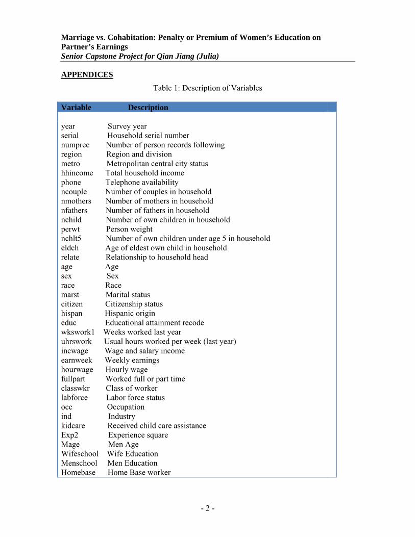
APPENDICES Table 1: Description of Variables
Variable Description year Survey year serial Household serial number numprec Number of person records following region Region and division metro Metropolitan central city status hhincome Total household income phone Telephone availability ncouple Number of couples in household nmothers Number of mothers in household nfathers Number of fathers in household nchild Number of own children in household perwt Person weight nchlt5 Number of own children under age 5 in household eldch Age of eldest own child in household relate Relationship to household head age Age sex Sex race Race marst Marital status citizen Citizenship status hispan Hispanic origin educ Educational attainment recode wkswork1 Weeks worked last year uhrswork Usual hours worked per week (last year) incwage Wage and salary income earnweek Weekly earnings hourwage Hourly wage fullpart Worked full or part time classwkr Class of worker labforce Labor force status occ Occupation ind Industry kidcare Received child care assistance Exp2 Experience square Mage Men Age Wifeschool Wife Education Menschool Men Education Homebase Home Base worker
Marriage vs. Cohabitation: Penalty or Premium of Women’s Education on Partner’s Earnings Senior Capstone Project for Qian Jiang (Julia)
- 3 -
REFERENCES (SIGLE-RUSHTON & MCLANAHAN, 2002) Amin, S., & Jepsen, L. K. (2005). The Impact of a Wife's Education on Her Husband's
Earnings in Malaysia. Journal of Economics, 31(2)
Astrom, J. (2009). The Effects of Spousal Educaiton on Individual Earnings – A Study of Married Swedish Couples. Department of Economics, Umea University.
Benham, L. (1974). Benefits of Women's Education within Marriage. Journal of Political Economy, Volumn 82 (1974).
Census Bureau. (2008). Retrieved from http://www.census.gov/population/www/pop-profile/natproj.html
U.S. Bureau of the Census. (2003). Retrieved from Estimated Median Age at First Marriage, by Sex: 1890 to Present: www.census.gov/population/socdemo/hh-fam/tabMS-2.pdf
U.S. Census. (2008). Retrieved from Education vs. Sex: www.uscensus.com
Census, U. B. (2007). Current Population Survey, 2007 Annual Social and economic . Retrieved from U.S. Bureau of Census: http://www.census.gov/apsd/techdoc/cps/cpsmar08.pdf
Chun, H., & Lee, I. (2001). Why Do Married Men Earn More: Productivity or Marriage Selection? Economic Inquiry , 307-319.
Edwards, T. (2009, Febuary 25). U.S. Census News. Retrieved from U.S. Census Bureau Press Release: http://www.census.gov/Press-Release/www/releases/archives/families_households/013378.html
Glick, J. E., Bean, F. D., & Van Hook, J. (1997). Immigration and Changing Patterns of Extended Family Household Structure in the United States 1970 -2990. Journal of Marriage and Family, 0022-2445.
Jepsen, L. K. (2005). The Relationship Between Wife's Education and Husband's Earning: Evidence from 1960 to 2000. Review of Economics of the Household , 197-214.
Juhn, C. a. (1997). Wages inequality and family labor supply. Journal of Labor Economics, volumn. 15(1), page 72-97.
Loh, E. S. (1995). Productivity Differences and the marriage Wage Premium fot White Males. The Journal of Human Resources, volumn 22, No. 2(spring).
Neuman, S., & Ziderman, A. (1990). Does A Woman's Education Affect Her Husband's Earnings? World Bank Working Papers, Augues 1990, WPS 464.
Marriage vs. Cohabitation: Penalty or Premium of Women’s Education on Partner’s Earnings Senior Capstone Project for Qian Jiang (Julia)
- 4 -
Pfeffer, J., & Ross, J. (1982). The Effects of Marriage and a Working Wife on Occupational and Wage Attainment, volume 27, No.1 (Mar., 1982), pp.66-80.
Schwartz, C. R., & Mare, R. D. (2005). Trendsin Educational Assortative Marriage From 1940 to 2003. Demography, volumne 42, number 4, November 2005, pp. 621-646.
Sigle-Rushton, W., & McLanahan, S. (2002). For Richer or Poorer? Marriage as an Anti-Poverty Strategy in the United States. Population , volume 57, pp. 509-526.
Skatun, J. D. (2004). Behind Every Well Paid Married Man: The Impact Of The Partner's Earning Opportunity. Australian Economic Papers, volume 43, pp.1-9, March 2004 .
Song, Y. (2007). The WOrking Spouse Penalty/ Premium and Married Women's Labor Supply, volume 5, Issue 3, page 279-304.
Wong, Y.-C. (1986). Entrepreneurship, Marriage, and Earnings. MIT Press in its journal Review of economics & Statistics, Volume 68, Issue 4, Page 693-699.
Work At Home Summary. (2005, September 22). Retrieved from Bureau of Labor Statistic: http://www.bls.gov/news.release/homey.nr0.htm