markov processes on the path space of the gelfand–tsetlin
TRANSCRIPT

Markov processes on the path space of theGelfand–Tsetlin graph and on its boundary
The MIT Faculty has made this article openly available. Please share how this access benefits you. Your story matters.
Citation Borodin, Alexei, and Grigori Olshanski. “Markov Processes on thePath Space of the Gelfand–Tsetlin Graph and on Its Boundary.”Journal of Functional Analysis 263, no. 1 (July 2012): 248–303.
As Published http://dx.doi.org/10.1016/j.jfa.2012.03.018
Publisher Elsevier
Version Author's final manuscript
Citable link http://hdl.handle.net/1721.1/101265
Terms of Use Creative Commons Attribution-Noncommercial-NoDerivatives
Detailed Terms http://creativecommons.org/licenses/by-nc-nd/4.0/

arX
iv:1
009.
2029
v1 [
mat
h.PR
] 1
0 Se
p 20
10
MARKOV PROCESSES ON THE PATH SPACE OF THE
GELFAND-TSETLIN GRAPH AND ON ITS BOUNDARY
ALEXEI BORODIN AND GRIGORI OLSHANSKI
Abstract. We construct a four-parameter family of Markov processes on infiniteGelfand-Tsetlin schemes that preserve the class of central (Gibbs) measures. Anyprocess in the family induces a Feller Markov process on the infinite-dimensionalboundary of the Gelfand-Tsetlin graph or, equivalently, the space of extreme char-acters of the infinite-dimensional unitary group U(∞). The process has a uniqueinvariant distribution which arises as the decomposing measure in a natural prob-lem of harmonic analysis on U(∞) posed in [Ols03]. As was shown in [BO05a], thismeasure can also be described as a determinantal point process with a correlationkernel expressed through the Gauss hypergeometric function.
Contents
1. Introduction 21.1. Gelfand-Tsetlin graph and its boundary 31.2. zw-measures 51.3. Doob’s transforms of N -fold products of birth and death processes 51.4. Main result 61.5. Markov process on Gelfand-Tsetlin schemes 61.6. Analytic continuation viewpoint 71.7. Pregenerator 81.8. Further questions 81.9. Organization of the paper 91.10. Acknowledgements 92. Abstract construction 92.1. Markov kernels 92.2. Feller kernels 102.3. Feller semigroups 102.4. Feller semigroups and Markov processes 102.5. Boundary 102.6. Feller boundary 112.7. Extension of semigroups to the boundary 112.8. Invariant measures 133. Specialization. Gelfand-Tsetlin graph 133.1. Spaces and links 13
1

2 ALEXEI BORODIN AND GRIGORI OLSHANSKI
3.2. Boundary 143.3. The boundary is Feller 164. Generalities on Markov chains on countable spaces 184.1. Regularity 184.2. Collapsibility 214.3. Infinitesimal generator 225. Semigroups on GTN 245.1. Case N = 1. Birth and death process on Z 245.2. The case of general N 276. Commutativity 316.1. Parameterization 316.2. Infinitesimal commutativity 326.3. From matrices of transition rates to semigroups 367. Invariant measures 387.1. zw-measures 397.2. Invariance 408. Stochastic dynamics on paths. General formalism 428.1. Overview 428.2. Construction of bivariate Markov chains 438.3. Construction of multivariate Markov chains 489. Stochastic dynamics on paths. Gelfand-Tsetlin graph 529.1. Central measures on paths and the boundary 529.2. Matrices of transition rates on GT
(N) 539.3. Regularity 559.4. Exclusion process 5510. Appendix 5710.1. Truncated Gelfand-Tsetlin graph 5710.2. The formal generator 60References 63
1. Introduction
This work is a result of interaction of two circles of ideas. The first one deals witha certain class of random growth models in two space dimensions [War07], [Nor10],[BF08+], [BG09], [BGR09+], [BK10] [Bor10+], while the second one addresses con-structing and analyzing stochastic dynamics on spaces of point configurations withdistinguished invariant measures that are often given by, or closely related to, de-terminantal point processes [BO06a], [BO06b], [BO09], [Ols10], [Ols10+].
Our main result is a construction of a Feller Markov process that preserves theso-called zw-measure on the (infinite-dimensional) space Ω of extreme characters

MARKOV PROCESSES . . . 3
of the infinite-dimensional unitary group U(∞). The four-parameter family of zw-measures arises naturally in a problem of harmonic analysis on U(∞) as the de-composing measures for a distinguished family of characters [Ols03]. A zw-measuregives rise to a determinantal point process on the real line with two punctures, andthe corresponding correlation kernel is given in terms of the Gauss hypergeometricfunction [BO05a]. Such point processes degenerate, via suitable limits and/or spe-cializations, to essentially all known one-dimensional determinantal processes withcorrelation kernels expressible through classical special functions.
The problem of constructing a Markov process that preserves a given determinan-tal point process with infinite point configurations has been addressed in [Spo87],[KT10], [Osa09+] for the sine process, in [KT09] for the Airy process, and in [Ols10+]for the Whittaker process describing the z-measures from the harmonic analysis onthe infinite symmetric group.
Our approach to constructing the infinite-dimensional stochastic dynamics differsfrom the ones used in previous papers. We employ the fact (of representation the-oretic origin) that the probability measures on Ω are in one-to-one correspondencewith central or Gibbs measures on infinite Gelfand-Tsetlin schemes that can also beviewed as stepped surfaces or lozenge tilings of a half-plane. The projections of azw-measure to suitably defined slices of the infinite schemes yield orthogonal polyno-mial ensembles with weight functions corresponding to hypergeometric Askey-Leskyorthogonal polynomials .
These orthogonal polynomials are eigenfunctions for a birth and death processon Z with quadratic jump rates; a standard argument then shows that the N -dimensional Askey-Lesky orthogonal polynomial ensemble is preserved by a Doob’sh-transform of N independent birth and death processes.
We further show that the Markov processes on the slices are consistent with re-spect to stochastic projections of the Nth slice to the (N−1)st one (these projectionsare uniquely determined by the Gibbs property). This consistency is in no way ob-vious, and we do not have a conceptual explanation for it. However, it turns out tobe essentially sufficient for defining the corresponding Markov process on Ω.
We do a bit more — using a continuous time analog of the general formalism of[BF08+] (which was based on an idea from [DF90]), we construct a Markov processon Gelfand-Tsetlin schemes that preserves the class of central (=Gibbs) measuresand that induces the same Markov process on Ω.
We now proceed to a more detailed description of our work.
1.1. Gelfand-Tsetlin graph and its boundary. Following [Wey39], for N ≥ 1define a signature of length N as an N -tuple of nonincreasing integers λ = (λ1 ≥· · · ≥ λN), and denote by GTN the set of all such signatures. Elements of GTN
parameterize irreducible representations of U(N) or GL(N,C), and they are oftencalled highest weights .

4 ALEXEI BORODIN AND GRIGORI OLSHANSKI
For λ ∈ GTN and ν ∈ GTN+1, we say that λ ≺ ν if νj+1 ≤ λj ≤ νj for allmeaningful values of indices. These inequalities are well-known to be equivalentto the condition that the restriction of the ν-representation of U(N + 1) to U(N)contains a λ-component.
Set GT =⊔
N≥1GTN , and equip GT with edges by joining λ and ν iff λ ≺ ν orν ≺ λ. This turns GT into a graph that we call the Gelfand-Tsetlin graph. A pathof length M ∈ 1, 2, . . . ∪ ∞ in GT is a length M sequence
λ(1) ≺ λ(2) ≺ . . . , λ(j) ∈ GTj.
Equivalently, such a path can be viewed as an array of numbersλ(j)i
satisfying
the inequalities λ(j+1)i+1 ≤ λ
(j)i ≤ λ
(j+1)i ; it is also called a Gelfand-Tsetlin scheme. An
interpretation of paths in GT in terms of lozenge tilings or stepped surfaces can befound in the introduction to [BF08+].
The Gelfand-Tsetlin schemes of lengthN parameterize basis vectors in theGelfand-Tsetlin basis of the irreducible representation of U(N) corresponding to λ(N), cf.[Zhe70]. Denote by DimN λ the number of such schemes with λ(N) = λ; this is alsothe dimension of the irreducible representation of U(N) corresponding to λ. It isessentially equal to the Vandermonde determinant in shifted coordinates of λ:
DimN(λ) = constN∏
1≤i<j≤N
(λi − i− λj + j).
A probability measure on infinite paths in GT is called central (or Gibbs) if anytwo finite paths with the same top end are equiprobable, cf. [Ker03]. Let PN bethe projection of such a measure to λ(N) ∈ GTN . Centrality is easily seen to beequivalent to the relation µN = µN+1Λ
N+1N , N ≥ 1, where µN and µN+1 are viewed
as row-vectors with coordinates µN(λ)λ∈GTNand µN+1(ν)ν∈GTN+1
, and
ΛN+1N (ν, λ) =
DimN(λ)
DimN(ν)1λ≺ν , λ ∈ GTN , ν ∈ GTN+1, (1.1)
is the stochastic matrix of cotransition probabilities . There is a one-to-one cor-respondence between central measures on GT and characters of U(∞) (equiva-lently, equivalence classes of unitary spherical representations of the Gelfand pair(U(∞)× U(∞), diagU(∞))), see [Ols03].
As shown in [Ols03], see also [Voi76], [VK82], [OO98], the space of all centralprobability measures is isomorphic to the space of all probability measures on theset Ω ⊂ R
4∞+2+ consisting of the sextuples ω = (α+, β+, α−, β−, δ+, δ−) ∈ R
4∞+2+
satisfying the conditions
α± = (α±1 ≥ α±
2 ≥ · · · ≥ 0), β± = (β±1 ≥ β±
2 ≥ · · · ≥ 0), δ± ≥ 0,∞∑
i=1
(α±i + β±
i ) ≤ δ±, β+1 + β−
1 ≤ 1.

MARKOV PROCESSES . . . 5
The set Ω is called the boundary of GT; its points parameterize the extremecharacters of U(∞). The map from central measures on GT to measures on Ωamounts to certain asymptotic relations described in Subsection 9.1 below.
1.2. zw-measures. Let z, z′, w, w′ be four complex parameters such that
(z + k)(z′ + k) > 0 and (w + k)(w′ + k) > 0 for any k ∈ Z (1.2)
and
z + z′ + w + w′ > −1 (1.3)
(note that (1.2) implies that z + z′ and w + w′ are real). For N ≥ 1, define aprobability measure on GTN by (below li = λi +N − i)
Mz,z,w,w′|N(λ) = constN∏
1≤i<j≤N
(li − lj)2
N∏
i=1
Wz,z′,w,w′(li), (1.4)
where
Wz,z′,w,w′(x) =1
Γ(z +N − x)Γ(z′ +N − x)Γ(w + 1 + x)Γ(w′ + 1 + x).
We call it the N th level zw-measure. It is the N -point orthogonal polynomialensemble with weight W ( · ), see e.g. [Kon05] and references therein for generalinformation on such ensembles.
One can show that the finite level zw-measures are consistent: For any N ≥ 1,Mz,z′,w,w′|N = Mz,z′,w,w′|N+1 Λ
N+1N . Therefore, the collection
Mz,z′,w,w′|N
N≥1
defines
a central measure on the paths in GT and a character of U(∞). For z′ = z, w′ = w,this character corresponds to a remarkable substitute for the nonexisting regularrepresentation of U(∞), see [Ols03] for details.
The corresponding measure Mz,z′,w,w′ on Ω is called the spectral zw-measure. Ifω = (α±, β±, δ±) ∈ Ω is distributed according to Mz,z′,w,w′ then the random pointprocess generated by the coordinates
12+ α+
i ,12− β+
i ,−12+ β−
i ,−12− α−
i
∞i=1
is determinantal, see [BO05a], [BO05b] for details.
1.3. Doob’s transforms of N-fold products of birth and death processes.
It is not hard to show that the first level zw-measure Mz,z′,w,w′|1 on GT1 = Z is thesymmetrizing measure for the bilateral birth and death process that from a pointx ∈ Z jumps to the right with intensity (x − u)(x− u′) and jumps to the left withintensity (x+ v)(x+ v′), where (u, u′, v, v′) = (z, z′, w, w′). Denote by D = Du,u′,v,v′
the corresponding matrix of transition rates.

6 ALEXEI BORODIN AND GRIGORI OLSHANSKI
More generally, we show that the Nth level zw-measure (1.4) is the symmetrizingmeasure for a continuous time Markov chain on GTN with transition rates
D(N)(λ, ν) =DimN(ν)
DimN(λ)
(D(l1, n1)1li=ni,i 6=1 +D(l2, n2)1li=ni,i 6=2 + . . .
+D(lN , nN )1li=ni,i 6=N
)− dN · 1λ=ν (1.5)
where lj = λj +N − j, nj = νj +N − j, 1 ≤ j ≤ N , dN is a suitable constant, andwe take (u, u′, v, v′) = (z +N − 1, z′ +N − 1, w, w′) in the definition of D.
Observe that D(N) can be viewed as a version of Doob’s h-transform of N copiesof the Markov chain defined by D with h( · ) = DimN ( · ). Note that in our case,DimN( · ) is an eigenfunction of the corresponding matrix of transition rates with anonzero eigenvalue.
For any N ≥ 1, let (PN(t))t≥0 be the Markov semigroup corresponding to thematrix D(N) of transition rates on GTN (we show that (PN(t))t≥0 is uniquely definedand it possesses the Feller property). The key fact that we prove is the consistency(or commutativity) relation
PN+1(t)ΛN+1N = ΛN+1
N PN (t), t ≥ 0, N ≥ 1.
Although this relation looks natural, we have no a priori reason to expect it tohold, and we verify it by a brute force computational argument.
1.4. Main result. We prove that for any (z, z′, w, w′) ∈ C4 subject to (1.2)-(1.3),there exists a unique Markov semigroup (P (t))t≥0 on Ω that preserves the spectralzw-measure Mz,z′,w,w′, and whose trace on GTN coincides with Doob’s transforms(PN(t))t≥0 introduced above. Moreover, the semigroup (P (t))t≥0 is Feller (it pre-serves C0(Ω), the Banach space of continuous functions vanishing at infinity; notethat the space Ω is locally compact).
By general theory, see e.g. [EK86, IV.2.7], this means that for any probabilitymeasure µ on Ω, there exists a Markov process on Ω corresponding to (P (t))t≥0 withinitial distribution µ and cadlag sample paths. We also show that Mz,z′,w,w′ is theunique invariant measure for this Markov process.
1.5. Markov process on Gelfand-Tsetlin schemes. Via the correspondence be-tween the probability measures on Ω and central measures on paths in GT, thesemigroup (P (t))t≥0 defines a Markov evolution of central measures. It is natural toask if there exists a Markov process on all probability measures on paths in GT thatagrees with the one we have when restricted to the central measures. We constructone such process; let us describe its transition rates.
Letλ(j)i
be a starting Gelfand-Tsetlin scheme. Then
• Each coordinate λ(k)i tries to jump to the right by 1 with rate
(λ(k)i − i− z + 1)(λ
(k)i − i− z′ + 1)

MARKOV PROCESSES . . . 7
and to the left by 1 with rate
(λ(k)i + k − i+ w)(λ
(k)i + k − i+ w′),
independently of other coordinates.
• If the λ(k)i -clock of the right jump rings but λ
(k)i = λ
(k−1)i−1 , the jump is blocked. If
its left clock rings but λ(k)i = λ
(k−1)i , the jump is also blocked. (If any of the two jumps
were allowed then the resulting set of coordinates would not have corresponded toa path in GT.)
• If the right λ(k)i -clock rings and there is no blocking, we find the greatest number
l ≥ k such that λ(j)i = λ
(k)i for j = k, k + 1, . . . , l, and move all the coordinates
λ(j)i
lj=k to the right by one. Given the change λ
(k)i 7→ λ
(k)i + 1, this is the minimal
modification of the initial Gelfand-Tsetlin scheme that preserves interlacing.
• If the left λ(k)i -clock rings and there is no blocking, we find the greatest number
l ≥ k such that λ(j)i+j−k = λ
(k)i for j = k, k + 1, . . . , l, and move all the coordinates
λ(j)i+j−k
lj=k to the left by one. Again, given the change λ
(k)i 7→ λ
(k)i − 1, this is the
minimal modification of the set of coordinates that preserves interlacing.
Since the update rule for each coordinate λ(k)i typically depends only on a few
surrounding coordinates, one can argue that we have a model of local random growth.It should be compared to the models treated in [BF08+], [BK10], where a similarblock-push mechanism was considered with constant jumps rates, and in [Bor10+],where the jump rates were also dependent on the location and numbering of thecoordinates.
The key new feature of the Markov process above is the absence of the limitshape phenomenon. Often taken for granted in local growth models, it is simplynonexistent here.
This fact becomes more apparent if we restrict ourselves to coordinates λ(j)1 j≥1
only. The evolution of this set of coordinates is also Markov, and it representsa kind of an exclusion process. Our results imply that this process has a uniqueequilibrium measure. Moreover, with respect to this measure, the asymptotic density
limj→∞ λ(j)1 /j is well-defined and random. It changes over time, and its distribution
is given by a solution to the classical Painleve VI (second order nonlinear) differentialequation, cf. [BD02].
1.6. Analytic continuation viewpoint. We have so far required the parameters(z, z′, w, w′) to satisfy (1.2) and (1.3). However, all the results would hold if (1.2) isreplaced by more general conditions, see [Ols03] for a precise description, with theonly difference being that the state spaces for our Markov processes would becomesmaller. In particular, if we choose
z = k ∈ Z≥0, z′ = k + a− 1, w = l ∈ Z≥0, w′ = l + b− 1, a, b > 0,

8 ALEXEI BORODIN AND GRIGORI OLSHANSKI
then we have to restrict ourselves to Gelfand-Tsetlin schemes with −l ≤ λ(j)i ≤ k for
all i, j ≥ 1. As the result, there are only k + l nontrivial parameters remaining onthe boundary, and (P (t))t≥0 turns into a finite-dimensional diffusion with an explicitsecond order differential operator as its generator. The equilibrium distribution (i.e.the spectral zw-measure) becomes the (k + l)-point Jacobi orthogonal polynomialensemble. See Subsection 10.1 for details.
One can thus think of our construction as of an analytic continuation in param-eters (k, l, a, b) of a very well understood finite-dimensional diffusion. This point ofview can be very fruitful: In [Ols10+] it was heavily exploited in the constructionand analysis of the Markov process preserving the spectral z-measure arising fromrepresentation theory of the infinite symmetric group. In that case, the startingpoint for analytic continuation was the Laguerre orthogonal polynomial ensembleand the corresponding diffusion, rather than the Jacobi one that we have here.
1.7. Pregenerator. As our construction of the semigroup (P (t))t≥0 is fairly inex-plicit, it is tempting to look for its alternative definition, for example, via a generator.
We were able to find a countable set of ‘coordinates’ on Ω such that the action ofthe generator of (P (t))t≥0 on polynomials in these coordinates is given by an explicitformal second order differential operator, see Subsection 10.2 below. However, it re-mains a challenge for us to derive properties of our Markov process (or its existence)from the resulting formula.
1.8. Further questions. As explained in [Ols03], the slices GTN can be embeddedinto the boundary so that as N →∞, their images form an increasingly fine grid inΩ. It is known that the Nth level zw-measures weakly converge to the spectral onesunder these embeddings. It would be desirable to prove a similar statement for theMarkov semigroups.
Verifying semigroup convergence would pave the way to proving that the equilib-rium Markov process on the boundary can also be described as a time-dependentdeterminantal point process. The fact that the dynamical correlation functions aredeterminantal on each GTN easily follows from known techniques, although deriv-ing useful formulas for the correlation kernel is a separate task. Another possiblecorollary of the semigroup convergence would be that the spectral zw-measure is asymmetrizing (not just an invariant) measure for (P (t))t≥0.
It seems important to continue the study of the pregenerator started in Subsection10.2. For example, it would be nice to understand if the space of polynomials in ourcoordinates is a core for the generator of the Markov process, and if not then howthat space should be modified.
Another way to benefit from investigating the generator would be to obtain aproof of the continuity of trajectories for our processes; we are only able to showthat the process has cadlag trajectories at the moment.

MARKOV PROCESSES . . . 9
All these questions and more have been settled in the case of the z-measurestreated in [Ols10+]. Unfortunately, key features of that model are not presenthere (like decomposition of the process into a one-dimensional one and a processon a compact set, or the existence of a convenient set of functions on the statespace isomorphic to the well-studied algebra of symmetric functions), and one wouldclearly need new ideas.
1.9. Organization of the paper. In Section 2 we present an abstract scheme ofconstructing a Markov semigroup on the boundary out of a consistent family ofsemigroups on the slices. In Section 3 we describe how the Gelfand-Tsetlin graphfits into this abstract scheme. Section 4 is a brief collection of general facts aboutcontinuous time Markov chains on countable spaces. Section 5 provides the con-struction of the Markov chains on GTN ’s. In Section 6 we verify the consistency ofthese Markov chains. Section 7 contains a brief description of the zw-measures. InSection 8 we develop a general formalism of building continuous time Markov chainson paths out of a consistent family of those on the slices. In Section 9 we apply thisformalism to our specific example and discuss the exclusion type processes. Section10 is an appendix without proofs; it contains a description of the finite-dimensionalcase of integral parameters z and w, and an explicit formula for the generator of ourMarkov process in certain coordinates.
1.10. Acknowledgements. A. B. was partially supported by NSF grants DMS-0707163 and DMS-1006991. G. O. was supported by the RFBR grant 08-01-00110,the RFBR-CNRS grant 10-01-93114, and the project SFB 701 of Bielefeld University.
2. Abstract construction
2.1. Markov kernels. For a more detailed exposition, see e.g. [Mey66, Ch. IX].Let E and E ′ be measurable spaces. A Markov kernel K : E → E ′ is a function
K(x,A), where x ∈ E and A ⊂ E ′ is a measurable subset, such that K(x, · ) is aprobability measure on E ′ and K( · , A) is a measurable function on E.
Let B(E) and B(E ′) denote the Banach spaces of real-valued bounded measurablefunctions with the sup-norm on E and E ′, respectively. A Markov kernelK : E → E ′
induces a linear operator B(E ′)→ B(E) of norm 1 via (Kf)(x) =∫E′ K(x, dy)f(y).
For two Markov kernels K1 : E → E ′ and K2 : E ′ → E ′′, their compositionK1 K2 : E → E ′′ is also a Markov kernel.
Denote byM( · ) the Banach space of signed measures of bounded variation withthe norm given by the total variation. Let M+( · ) be the cone of finite positivemeasures, and letMp( · ) be the simplex of the probability measures.
A Markov kernel K : E → E ′ also induces a linear operatorM(E) →M(E ′) ofnorm 1 via (µK)(dy) =
∫Eµ(dx)K(x, dy). This operator mapsM+(E) toM+(E
′)and Mp(E) to Mp(E
′). Note that δxK = K(x, · ), where δx is the Dirac delta-measure at x ∈ E.

10 ALEXEI BORODIN AND GRIGORI OLSHANSKI
The spaceM(E) (and henceM+(E) andMp(E)) is equipped with a σ-algebraof measurable sets: Any preimage of a Borel set under the map µ 7→ µ(A) fromM(E) to R for any measurable A is measurable.
2.2. Feller kernels. Let E and E ′ be locally compact topological spaces with count-able bases. Let us take Borel σ-algebra as the σ-algebra of measurable sets for bothof them.
Let C( · ) ⊂ B( · ) be the Banach space of bounded continuous functions, and letC0( · ) ⊂ C( · ) be its subspace of functions that tend to 0 at infinity.
Definition 2.1. A Markov kernel K : E → E ′ is called Feller if the induced mapB(E ′)→ B(E) maps C0(E
′) to C0(E).
Note that different authors may use different (nonequivalent) definitions for theFeller property.
The convenience of the space C0( · ) is based on the fact that this space is separable(as opposed to C( · ) which is not separable, except in the case when the initialtopological space is compact), andM( · ) is its Banach dual.
2.3. Feller semigroups. A Markov semigroup is a family of Markov kernels P (t) :E → E, where t ≥ 0, P (0) = 1 (in the obvious sense), and P (s)P (t) = P (s + t).Such a semigroup induces a semigroup of linear operators in B(E) as well as asemigroup of linear operators inMp(E), see above.
We say that a Markov semigroup (P (t))t≥0 is Feller if• E is a locally compact topological space with countable base;• the corresponding operator semigroup in B(E) preserves C0(E);• the function t 7→ P (t) is strongly continuous, i.e. t 7→ P (t)f is a continuous mapfrom [0,+∞) to C0(E) for any f ∈ C0(E) (an equivalent condition is the continuityat t = 0).
2.4. Feller semigroups and Markov processes. For more details, see e.g. [EK86,IV.2.7].
Let E be a locally compact separable metric space, and let (P (t))t≥0 be a Fellersemigroup on E. Then for each µ ∈ Mp(E), there exists a Markov process corre-sponding to (P (t))t≥0 with initial distribution µ and cadlag sample paths. Moreover,this process is strongly Markov with respect to the right-continuous version of itsnatural filtration.
2.5. Boundary. Let E1, E2, . . . be a sequence of measurable spaces linked by Markovkernels
ΛN+1N : EN+1 → EN , N = 1, 2, . . . .
Assume that we have another measurable space E∞ and Markov kernels
Λ∞N : E∞ → EN , N = 1, 2, . . . ,

MARKOV PROCESSES . . . 11
such that the natural commutativity relations hold:
Λ∞N+1 Λ
N+1N = Λ∞
N , N = 1, 2, . . . . (2.1)
The kernels ΛN+1N induce the chain of maps, cf. 2.1,
· · · →Mp(EN+1)→Mp(EN )→ · · · →Mp(E2)→Mp(E1), (2.2)
and we can define the projective limit lim←−Mp(EN) with respect to these maps. By
definition, it consists of sequences of measures (µN)N≥1, µN ∈ Mp(EN), that arelinked by the maps from (2.2). The space lim
←−Mp(EN ) is measurable; the σ-algebra
of measurable sets is generated by the cylinder sets in which µN must lie inside ameasurable subset ofMp(EN), and all other coordinates (µk)k 6=N , are unrestricted.
Observe that to any µ∞ ∈Mp(E∞) one can assign an element of lim←−Mp(EN) by
setting µN equal to the image of µ∞ under the mapMp(E∞)→Mp(EN ) induced byΛ∞
N . The commutativity relations (2.1) ensure that the resulting sequence (µN)N≥1
is consistent with (2.2).
Definition 2.2. We say that E∞ is a boundary of the sequence (EN )N≥1 if the mapMp(E∞)→ lim
←−Mp(EN ) described in the previous paragraph is a bijection and also
an isomorphism of measurable spaces.
2.6. Feller boundary. In the setting of the previous subsection, let us furtherassume that (EN )N≥1 and E∞ are locally compact topological spaces with countablebases, and all the links (ΛN+1
N )N≥1, (Λ∞N )N≥1 are Feller kernels, cf. Subsection 2.2.
Then if E∞ satisfies Definition 2.2, we shall call it the Feller boundary for (EN )N≥1.According to Subsection 2.2, the links (Λ∞
N )N≥1 induce linear operators C0(EN)→C0(E∞).
Lemma 2.3. The union of images of these maps over all N ≥ 1 is dense in theBanach space C0(E∞).
Proof. Since M(E∞) is the Banach dual to C0(E∞), it suffices to verify that ifµ ∈M(E∞) kills all functions in our union then µ = 0.
Assume µ is a signed measure on E∞ that kills the image of C0(EN), N ≥ 1.This is equivalent to saying that µK∞
N = 0 for all N ≥ 1. We can represent µ asdifference of finite positive measures
M = αµ′ − βµ′′, µ′, µ′′ ∈Mp(E∞), α, β ≥ 0.
Hence, αµ′K∞N = βµ′′K∞
N for all N ≥ 1. Since µ′K∞N and µ′′K∞
N are in Mp(EN),we must have α = β, and µ′K∞
N = µ′′K∞N . Definition 2.2 implies µ′ = µ′′, thus
µ = 0.
2.7. Extension of semigroups to the boundary. In the setting of Subsection2.5, assume that for any N ≥ 1, we have a Markov semigroup (PN (t))t≥0 on EN ,and these semigroups are compatible with the links:
PN+1(t) ΛN+1N = ΛN+1
N PN(t), t ≥ 0, N = 1, 2, . . . . (2.3)

12 ALEXEI BORODIN AND GRIGORI OLSHANSKI
Proposition 2.4. In the above assumptions, there exists a unique Markov semigroupP (t) on E∞ such that
P (t) Λ∞N = Λ∞
N PN(t), t ≥ 0, N = 1, 2, . . . . (2.4)
If E∞ is Feller (cf. Subsection 2.6) and (PN(t))t≥0 is a Feller semigroup for anyN ≥ 1, then (P (t))t≥0 is also a Feller semigroup.
Proof. Denote by δx the delta-measure at a point x ∈ E∞. To construct the semi-group (P (t))t≥0, we need to define, for any t ≥ 0, a probability measure P (t; x, · )on E∞. This measure has to satisfy
P (t; x, · )Λ∞N = δx(Λ
∞N PN(t)), N ≥ 1.
The right-hand side defines a sequence of probability measures on EN ’s, and (2.1),(2.3) immediately imply that these measures are compatible with maps (2.2). Hence,we obtain an element of lim
←−Mp(EN), which defines, by definition of the boundary,
a probability measure on E∞. The dependence of this measure on x is measurablesince this is true for any of its coordinates.
Thus, we have obtained a Markov kernel P (t) which satisfies
δx(P (t) Λ∞N ) = δx(Λ
∞N PN(t)), N ≥ 1,
which is equivalent to (2.4).To verify the semigroup property (Chapman-Kolmogorov equation) for (P (t))t≥0
it suffices to check that
(P (s) P (t)) Λ∞N = P (s+ t) Λ∞
N , s, t ≥ 0, N ≥ 1,
and this immediately follows from (2.4) and the corresponding relation for (PN(t))t≥0.The uniqueness is obvious since P (t) is uniquely determined by (P (t) Λ∞
N )N≥1
that are given (2.4).Finally, let us prove the Feller property assuming that the boundary is Feller and
all (PN (t))t≥0 are Feller.We need to show that for f ∈ C0(E∞) we have P (t)f ∈ C0(E∞), and that P (t)f
is continuous in t in the topology of C0(E∞). Both properties can be verified ona dense subset. Lemma 2.3 then shows that it suffices to consider f of the formf = Λ∞
N fN with fN ∈ C0(EN). By (2.4)
P (t)f = P (t)(Λ∞N fN) = Λ∞
N (PN(t)fN ),
which is in C0(E∞) because Λ∞N and PN(t) are Feller. The continuity in t is obvious
as PN(t)fN is continuous in t, and Λ∞N : C0(EN)→ C0(E∞) is a contraction.
It is worth noting that our definition of the semigroup P (t) is nonconstructive:We are not able to describe P (t; x,A) explicitly, and we have to appeal to theisomorphism in Definition 2.2 instead. Thus, the difficulty in making P (t) explicitis hidden in the implicit nature of that isomorphism.

MARKOV PROCESSES . . . 13
2.8. Invariant measures. In the setting of Subsection 2.5, assume that for anyN ≥ 1, there exists µN ∈Mp(EN) such that µNPN(t) = µN (i.e., µN is an invariantmeasure for (PN(t))t≥0). If we assume that µN ’s are compatible with the links,
µN+1ΛN+1N = µN , N ≥ 1,
then, via Definition 2.2, they yield a measure µ ∈ Mp(E∞) such that µΛ∞N = µN
for any N ≥ 1. Note that µ is uniquely determined by its coordinates.One easily sees that µ is invariant with respect to (P (t))t≥0. Indeed,
(µP (t))Λ∞N = (µΛ∞
N )PN(t) = µNPN(t) = µN = µΛ∞N .
Moreover, if µN is a unique invariant measure for (PN(t))t≥0 for any N ≥ 1 thenthe invariant measure for (P (t))t≥0 is unique too as its convolution with Λ∞
N mustcoincide with µN .
3. Specialization. Gelfand-Tsetlin graph
3.1. Spaces and links. Let N be a positive integer. A signature λ of length Nis an N -tuple of weakly decreasing integers: λ = (λ1 ≥ · · · ≥ λN) ∈ ZN . Denoteby GTN the set of all signatures of length N (the notation GT is explained below).This countable set will serve as our space EN from the previous section.
Signatures of length N parameterize irreducible representations of the unitarygroup U(N) and are often referred to as highest weights , cf. [Wey39], [Zhe70]. Forλ ∈ GTN denote the corresponding representation by πλ, and denote by DimN λ thedimension of the corresponding linear space. It is well known that
DimN λ =
∏1≤i<j≤N(λi − i− λj + j)
∏N−1i=1 i!
, λ ∈ GTN .
Define a matrix[ΛN+1
N (λ, ν)]λ∈GTN+1, ν∈GTN
with rows parameterized by GTN+1
and columns parameterized by GTN via
ΛN+1N (λ, ν) =
N ! ·
∏1≤i<j≤N(νi − i− νj + j)
∏1≤i<j≤N+1(λi − i− λj + j)
, if ν ≺ λ,
0, otherwise,
where the notation ν ≺ λ stands for interlacing:
ν ≺ λ ⇐⇒ λ1 ≥ ν1 ≥ λ2 ≥ ν2 ≥ · · · ≥ νN ≥ λN+1.
Note that the nonzero entries of ΛN+1N can also be written in the form
ΛN+1N (λ, ν) =
DimN ν
DimN+1 λ. (3.1)
It is not hard to show that ΛN+1N is a stochastic matrix:
∑ν∈GTN
ΛN+1N (λ, ν) = 1
for any λ ∈ GTN+1. Indeed, DimN+1 λ is equal to the number of the sequences

14 ALEXEI BORODIN AND GRIGORI OLSHANSKI
(known as Gelfand-Tsetlin schemes , thus the notation GT)
λ(1) ≺ λ(2) ≺ · · · ≺ λ(N+1) = λ, λ(j) ∈ GTj ,
and ΛN+1N (λ, ν) is the fraction of the sequences with λ(N) = ν. The stochasticity
also follows from the branching rule for the representations of unitary groups: Forany λ ∈ GTN+1,
πλ|U(N) ∼⊕
ν∈GTN : ν≺λ
πν .
The matrices ΛN+1N viewed as Markov kernels ΛN+1
N : GTN+1 → GTN are ourlinks, cf. Subsection 2.5. Set GT =
⊔N≥1GTN . We endow GT with the structure
of a graph: Two vertices λ and ν are joined by an edge if and only if ν ≺ λ or λ ≺ ν.This graph is called the Gelfand-Tsetlin graph, and the matrix elements of the linksare often called cotransition probabilities for this graph, cf. [Ker03].
3.2. Boundary. let R+ ⊂ R be the set of nonnegative real numbers and R∞+ be the
product of countably many copies of R+. Consider the space
R4∞+2+ := R
∞+ × R
∞+ × R
∞+ × R
∞+ × R+ × R+
and equip it with the product topology. We choose E∞ to be the closed subsetΩ ⊂ R
4∞+2+ consisting of the sextuples
ω = (α+, β+, α−, β−, δ+, δ−) ∈ R4∞+2+
satisfying the conditions
α± = (α±1 ≥ α±
2 ≥ . . . ), β± = (β±1 ≥ β±
2 ≥ . . . ), δ± ≥ 0,∞∑
i=1
(α±i + β±
i ) ≤ δ±, β+1 + β−
1 ≤ 1.
One easily sees that Ω is a locally compact metrizable topological space with acountable base. We endow Ω with the corresponding Borel structure which makesΩ a measurable space.
It will be convenient to use the notation
γ± = δ± −
∞∑
i=1
(α±i + β±
i ) ≥ 0.
Define the projections/links Λ∞N : Ω→ GTN , N ≥ 1, by
Λ∞N (ω, λ) = DimN λ · det
[ϕλi−i+j
]Ni,j=1
, ω ∈ Ω, λ ∈ GTN , (3.2)
where ϕn+∞n=−∞ are the Laurent coefficients of the function (|u| = 1)
Φω(u) := eγ+(u−1)+γ−(u−1−1)
∞∏
i=1
1 + β+i (u− 1)
1− α+i (u− 1)
1 + β−i (u
−1 − 1)
1− α−i (u
−1 − 1)=
+∞∑
n=−∞
ϕnun.
(3.3)

MARKOV PROCESSES . . . 15
Theorem 3.1. The space E∞ = Ω is the boundary of the chain of spaces (EN =GTN)N≥1 with links as above in the sense of Definition 2.2.
Proof. This result is essentially proved in §9 of [Ols03]; we provide below somenecessary additional comments.
Let us abbreviate ∆N = Mp(GTN) and ∆ = lim←−Mp(GTN) = lim
←−∆N . As in
[Ols03] we embed ∆ into the vector space of all real-valued functions on the set ofvertices of the Gelfand–Tsetlin graph. That space is endowed with the topology ofpointwise convergence, and ∆ inherits this topology. The measurable structure of∆ is the Borel structure corresponding to this topology.
Obviously, ∆ is a convex set; let Ex∆ ⊂ ∆ denote the subset of extreme points.Theorem 9.2 in [Ols03] (which is based on Choquet’s theorem) says that Ex∆ is aBorel subset of ∆, and each point of ∆ is uniquely representable by a probabilityBorel measure concentrated on Ex∆. On the other hand, it is readily seen that,conversely, any probability Borel measure on ∆ (in particular, on Ex∆) representsa point of ∆, the barycenter of that measure. This gives us a bijection betweenMp(Ex∆) and ∆.
The next step consists in identifying the abstract set Ex∆ with the concretespace Ω. This is achieved with the help of Theorem 1.3 in [Ols03]. Namely, asis pointed out in the proof of Theorem 9.1 in [Ols03], there is a natural one-to-one correspondence between the points of Ex∆ and the extreme characters of theinfinite-dimensional unitary group U(∞), which in turn are parameterized by thepoints of the space Ω, see Theorem 1.3 in [Ols03].
Then we have to verify that the embedding Ω→ ∆ induced by the identificationΩ = Ex∆ is given by the kernels Λ∞
N . This is shown by the computation in [Voi76].We have thus constructed a bijective mapMp(Ω) → ∆, and it remains to prove
that it is a Borel isomorphism. As shown in the proof of Theorem 8.1 of [Ols03],the map ω 7→ Λ∞
N (ω, λ) is continuous for every N = 1, 2, . . . and every λ ∈ GTN .This implies that the map Mp(Ω) → ∆ is Borel. To show that the inverse mapis also Borel one can apply an abstract result (Theorem 3.2 in [Mack57]), whichasserts that a Borel one-to-one map of a standard Borel space onto a subset of acountably generated Borel space is a Borel isomorphism. This result is applicable inour situation, since the Borel structure of Ω is standard, so that the induced Borelstructure onMp(Ω) is standard, too.
Remark 3.2. Observe that the maps on (GTN)N≥1 consisting of shifts of all coor-dinates of signatures by 1,
λ = (λ1, . . . , λN) 7→ λ = (λ1 = λ1 + 1, . . . , λN = λN + 1),
leave the links intact: ΛN+1N (λ, ν) = ΛN+1
N (λ, ν). There is also a correspondinghomeomorphism of Ω, which amounts to the multiplication of the function Φω(u)

16 ALEXEI BORODIN AND GRIGORI OLSHANSKI
by u: For ω = (α±, β±, δ±) ∈ Ω define ω = (α±, β±, δ±) ∈ Ω by
α± = α±, δ± = δ±,
β+1 = 1− β−
1 , (β+2 , β
+3 , . . . ) = (β+
1 , β+2 , . . . ), (β−
1 , β−2 , . . . ) = (β−
2 , β−3 , . . . )
(note that β+1 ≥ β+
2 because β+1 + β−
1 ≤ 1). Then (3.2) and the relation
u(1 + β−1 (u
−1 − 1)) = 1 + (1− β−1 )(u− 1)
show that Λ∞N (ω, λ) = Λ∞
N (ω, λ) for any λ ∈ GTN and N ≥ 1.This automorphism of the Gelfand-Tsetlin graph and its boundary has a repre-
sentation theoretic origin, cf. Remark 1.5 in [Ols03] and Remark 3.7 in [BO05a].
3.3. The boundary is Feller. Following definitions of Subsection 2.6, in order toshow that E∞ = Ω is a Feller boundary of the chain (EN = GTN)N≥1 we need toverify two statements:• the spaces (EN)N≥1 and E∞ are locally compact topological spaces with count-able bases;• the links (ΛN+1
N )N≥1 and (Λ∞N )N≥1 are Feller kernels.
The first statement is obvious from the definitions. The goal of this subsection isto prove the second one.
Proposition 3.3. For any N ≥ 1, the linear operator B(GTN) → B(GTN+1) in-duced by the Markov kernel ΛN+1
N maps C0(GTN ) to C0(GTN+1).
Proof. As the norm of the linear operator in question is equal to 1 and C0( · ) is aclosed subspace of B( · ), it suffices to check that the images of all delta-functions onGTN are in C0(GTN+1).
For a ν ∈ GTN , let δν be the delta-function on GTN concentrated at ν. Then forλ ∈ GTN+1
(ΛN+1N δν)(λ) =
N ! ·
∏1≤i<j≤N(νi − i− νj + j)
∏1≤i<j≤N+1(λi − i− λj + j)
, if ν ≺ λ,
0, otherwise.
If we assume that (ΛN+1N δν)(λ) 6= 0 then λ → ∞ is equivalent to either λ1 → +∞,
or λN+1 → −∞, or both; all other coordinates must remain bounded because of theinterlacing condition ν ≺ λ. But then it is immediate that at least one of the factorsin the denominator in (ΛN+1
N δν)(λ) tends to infinity. Thus, for any fixed ν ∈ GTN ,(ΛN+1
N δν)(λ)→ 0 as λ→∞ as needed.
Proposition 3.4. For any N ≥ 1, the linear operator B(GTN )→ B(Ω) induced bythe Markov kernel Λ∞
N maps C0(GTN) to C0(Ω).
Proof. As in the proof of Proposition 3.3, it suffices to prove that for any ν ∈ GTN ,(Λ∞
N δν)(ω) = Λ∞N (ω, λ) belongs to C0(Ω) as a function in ω ∈ Ω. The proof of

MARKOV PROCESSES . . . 17
continuity of Λ∞N (ω, λ) in ω is contained in the proof of Theorem 8.1 of [Ols03]. It
remains to show that Λ∞N (ω, λ)→ 0 as ω →∞. Note that ω → ∞ is equivalent to
δ+ + δ− → +∞.Observe that the coefficients ϕn = ϕn(ω) from (3.3) can be written as
ϕn(ω) =1
2πi
∮
|u|=1
Φω(u)du
un+1, n ∈ Z. (3.4)
Note that |Φω(u)| ≤ 1 on the unit circle |u| = 1, because the modulus of each of the
factors (1− α±i (u
±1 − 1))−1, (1 + β±i (u
±1 − 1)), and eγ±(u±1−1) is ≤ 1.
We are going to prove that for any fixed n ∈ Z, ϕn → 0 as ω →∞; by (3.2) thiswould imply the needed claim.
Let us assume the converse, i.e. assume that there exist c > 0, n0 ∈ Z, and asequence ω(k)k≥1 ⊂ Ω with limk→∞ ω(k) = ∞, such that ϕn0(ω(k)) > c. Letus denote by (α±(k), β±(k), δ±(k)) the coordinates of ω(k). We will now collectinformation about ω(k) that will eventually lead to a contradiction.
Step 1. We must have supk≥1 α±1 (k) <∞. Indeed, if there is a subsequence kmm≥1
such that α±1 (km) →∞, then along this subsequence (1 − α±
1 (u±1 − 1))−1 tends to
zero uniformly on any compact subset of u : |u| = 1 \ u = 1, which implies thatthe right-hand side of (3.4) tends to zero.
Let us fix A > 0 such that supk α±1 (k) ≤ A.
Step 2. Assume ω ranges over the subset of elements of Ω with α±1 ≤ A and β±
1 ≤12.
Then for any ǫ > 0,
limδ++δ−→∞
Φω(u) = 0 uniformly on u ∈ C : |u| = 1, ℜu ≤ 1− ǫ.
Indeed, for u on the unit circle with ℜu ≤ 1− ǫ we have elementary estimates
|1 + β(u− 1)|2 = (1− β)2 + β2 + 2β(1− β)ℜu
= 1− 2β(1− β)(1−ℜu) ≤ 1− 2β(1− β)ǫ ≤ 1− βǫ ≤ e−βǫ, (3.5)
|1− α(u− 1)|−2 = (1 + 2α(1 + α)(1−ℜu))−1
≤ (1 + 2α(1 + α)ǫ)−1 ≤ (1 + 2αǫ)−1 ≤ e− constαǫ, (3.6)
|eγ+(u−1)+γ−(u−1−1)|2 = e−2(γ++γ−)(1−ℜu) ≤ e−2(γ++γ−)ǫ,
with a suitable constant const > 0 (that depends on A). Thus, if
δ+ + δ− = γ+ + γ− +
∞∑
i=1
(α+i + β+
i + α−i + β−
i )→∞

18 ALEXEI BORODIN AND GRIGORI OLSHANSKI
then at least one of the right-hand sides in these estimates yields an infinitesimallysmall contribution, and Φω(u) must be small. Thus, under the above assumptionson ω, we see that ω →∞ implies ϕn(ω)→ 0 uniformly on n ∈ Z.
Step 3. Now we get rid of the restriction β±1 ≤
12. Set
B±(k) = #i ≥ 1 | β±i (k) >
12.
Since for any k ≥ 1 we have β+1 (k) + β−
1 (k) ≤ 1, at least one of the numbers B±(k)is equal to 0. The statement of Step 2 shows that for any subsequence ωkm of oursequence ω(k), we must have B+(km)+B−(km)→∞. Hence, possibly passing toa subsequence and switching + and −, we may assume that B+(k)→∞ as k →∞.
Using the identity (cf. Remark 3.2)
1 + β(u− 1) = u(1 + (1− β)(u−1 − 1))
B+(k) times on Φω(k)(u), we see that ϕn0(ω(k)) = ϕn0−B+(k)(ω(k)), where ω(k)is obtained from ω(k) as follows: Each β+-coordinate of ω(k) that is > 1/2 istransformed into a β− coordinate of ω(k) equal to 1 minus the original β+-coordinate;all other coordinates are the same (equivalently, the function Φω(k)(u) is multiplied
by u−B(k)). Let (α±(k), β±(k), γ±(k), δ±(k)) be the coordinates of ω(k).
Step 4. Since no β-coordinates of ω(k) are greater than 1/2, the argument of Step
2 implies that if δ+(k) + δ−(k) → ∞ then ϕn0(ω(k)) = ϕn0−B+(k)(ω(k)) → 0 as
k →∞, which contradicts our assumption. Hence, δ+(k) + δ−(k) is bounded.Let us deform the integration contour in (3.4) to |u| = R with A/(1+A) < R < 1.
Using the estimates (for |u| = R, 0 ≤ α ≤ A, 0 ≤ β ≤ 1/2)
|1 + β(u±1 − 1)| ≤ 1 + β|u±1 − 1| ≤ econst1 β,
|1− α(u±1 − 1)|−1 ≤ |1− α(R±1 − 1)|−1 ≤ econst2 α,
|eγ(u±1−1)| ≤ econst3 γ
with suitable constj > 0, j = 1, 2, 3, we see that |Φω(k)(u)| ≤ econst4(δ+(k)+δ−(k)), for
a const4 > 0, which remains bounded. On the other hand, the factor u−n0−1+B+(k)
in the integral representation (3.4) for ϕn0−B+(k)(ω(k)) tends to 0 uniformly in u,|u| = R < 1. Hence, ϕn0(ω(k)) = ϕn0−B+(k)(ω(k))→ 0 as k →∞, and the proof ofProposition 3.4 is complete.
4. Generalities on Markov chains on countable spaces
4.1. Regularity. Let E be a countable set, and let (P (t))t≥0 be a Markov semigroupon E. Each P (t) may be viewed as a matrix with rows and columns marked byelements of E; its entries will be denoted by P (t; a, b), a, b ∈ E. By definition,P (t; a, b) is the probability that the process will be in the state b at the time momentt conditioned that it is in the state a at time 0. Thus, all matrix elements ofP (t) are nonnegative, and their sum is equal to 1 along any row - the matrix P (t)

MARKOV PROCESSES . . . 19
is stochastic. The transition matrices P (t) also satisfy the Chapman-Kolmogorovequation P (s)P (t) = P (s+ t).
Assume that there exists an E ×E matrix Q such that
P (t; a, b) = 1a=b +Q(a, b)t+ o(t), t ↓ 0. (4.1)
This relation implies that Q(a, b) ≥ 0 for a 6= b and Q(a, a) ≤ 0. Further, we willalways assume that
∑
b6=a
Q(a, b) = −Q(a, a) for any a ∈ E.
This is the infinitesimal analog of the condition∑
b∈E P (t; a, b) = 1.It is well known that the Chapman-Kolmogorov equation implies that P (t) satis-
fies Kolmogorov’s backward equation
d
dtP (t) = QP (t), t > 0, (4.2)
with the initial condition
P (0) ≡ Id . (4.3)
Under certain additional conditions, P (t) will also satisfy Kolmogorov’s forwardequation
d
dtP (t) = P (t)Q, t > 0. (4.4)
One says that Q is the matrix of transition rates for (P (t))t≥0.One often wants to define a Markov semigroup by giving the transition rates.
However, it may happen that this does not specify the semigroup uniquely (thenthe backward equation has many solutions). Uniqueness always holds if E is finiteor, more generally, if E is infinite but the diagonal entries Q(a, a) are bounded.However, these simple conditions do not suit our purposes, and we need to go alittle deeper into the general theory.
Let us write Q in the form Q = −q + Q, where −q is the diagonal part of Q and
Q is the off-diagonal part of Q. In other words,
q(a, b) = −Q(a, a)1ab, Q(a, b) =
Q(a, b), a 6= b,
0, a = b.
Define P [n](t) recursively by
P [0](t) = e−tq, P [n](t) =
∫ t
0
e−τqQP [n−1](t− τ) dτ, n ≥ 1,
and set
P (t) =
∞∑
n=0
P [n](t), t ≥ 0.

20 ALEXEI BORODIN AND GRIGORI OLSHANSKI
Theorem 4.1 ([Fel40]). (i) The matrix P (t) is substochastic (i.e., its elements arenonnegative and
∑b P (t; a, b) ≤ 1). Its elements are continuous in t ∈ [0,+∞) and
differentiable in t ∈ (0,+∞), and it provides a solution of Kolmogorov’s backwardand forward equations (4.2), (4.4) with the initial condition (4.3).
(ii) P (t) also satisfies the Chapman-Kolmogorov equation.(iii) P (t) is the minimal solution of (4.2) (or (4.4)) in the sense that for any
other solution P (t) of (4.2) (or (4.4)) with the initial condition (4.3) in the class ofsubstochastic matrices, one has P (t; a, b) ≥ P (t; a, b) for any a, b ∈ E.
Corollary 4.2. If the minimal solution P (t) is stochastic (the sums of matrix ele-ments along the rows are all equal to 1 ) then it is the unique solution of (4.2) (or(4.4)) with the initial condition (4.3) in the class of substochastic matrices.
If the minimal solution P (t) is stochastic one says that the matrix of transitionrates Q is regular , cf. Proposition 4.3.
Observe that the construction of P (t) is very natural: the summands P [n](t; a, b)are the probabilities to go from a to b in n jumps. The condition of P (t) beingstochastic exactly means that we cannot make infinitely many jumps in a finiteamount of time.
A much more detailed account of Markov chains on countable sets can be founde.g. in [And91].
Later on we will need the following sufficient condition for P (t) to be stochastic.For any finite X , X ⊂ E, a ∈ X , denote by Ta,X the time of the first exit from
X under the condition that the process is in a at time 0. Formally, we can modify
E and Q by contracting all the states b ∈ E \ X into one absorbing state b with
Qb,c ≡ 0 for any c ∈ X ∪b. We obtain a process with a finite number of states for
which the solution P (t) of the backward equation is unique. Then Ta,X is a randomvariable with values in (0,+∞] defined by
ProbTa,X ≤ t = P (t; a, b).
Proposition 4.3. Assume that for any a ∈ E and any t > 0, ε > 0, there existsa finite set X(ε) ⊂ E such that ProbTa,X(ε) ≤ t ≤ ε. Then the minimal solution
P (t) provided by Theorem 4.1 is stochastic.
Proof. Consider the modified process on the finite state space X(ε)∪ b described
above. Since its transition matrix P (t) is stochastic,∑
b∈X(ε)
P (t; a, b) = 1− P (t; a, b) ≥ 1− ε.
The construction of the minimal solution as the sum of P [n]’s, see above, immediately
implies that P (t; a, b) ≥ P (t; a, b). Thus,∑
b P (t; a, b) ≥ 1− ε for any ε > 0.

MARKOV PROCESSES . . . 21
4.2. Collapsibility. In what follows we will also need a result on collapsibility orlumpability of Markov chains on discrete spaces. Let us describe it.
Let E =⊔
i∈I Ei be a partition of the countable set E on disjoint subsets. Assumewe are given a matrix QE of transition rates on E and a matrix QI of transitionrates on I such that
∑
b∈Ej
QE(a, b) = QI(i, j) for any a ∈ Ei, i, j ∈ I. (4.5)
Denote
qE(a) = −QE(a, a), qI(i) = −QI(i, i).
For any i ∈ I, let Qi be a matrix of transition rates on Ei defined by
Qi(a, b) = QE(a, b) if a 6= b, a, b ∈ Ei,
qi(a) = −Qi(a, a) =∑
b∈Ei,b6=a
Qi(a, b), a ∈ Ei.
Observe that qE(a) = qi(a) + qI(i) for any a ∈ Ei.Denote by PE(t) and P I(t) the minimal solutions of Kolmogorov’s equations for
QE and QI , respectively.
Proposition 4.4. Assume that for any i ∈ I, Qi is regular. Then for any t ≥ 0∑
b∈Ej
PE(t; a, b) = P I(t; i, j) (4.6)
for any i, j ∈ I and any a ∈ Ei. In particular, if QI is regular then so is QE andvice versa.
Proof. Let us use notations q, Q, and P [n] for the diagonal and off-diagonal parts ofthe matrices of transition rates, and for the nth terms in the series representationsof minimal solutions, respectively.
The hypothesis means that the identity
∑
b∈Ei
∞∑
n=0
P[n]i (t; a, b) = 1, a ∈ Ei, i ∈ I,
holds, where
P[n]i (t) =
∫
0≤t1≤···≤tn≤t
e−t1qiQie−(t2−t1)qiQi · · · e
−(tn−tn−1)qiQie−(t−tn)qidt1 · · · dtn
and P(0)i (t) = e−tqi . Using the fact that qi( · ) = qE( · ) − qI(i) on Ei, rewrite this
identity as

22 ALEXEI BORODIN AND GRIGORI OLSHANSKI
∑
b∈Ei
∞∑
n=0
∫
0≤t1≤···≤tn≤t
(e−t1qE1Ei
QE 1Eie−(t2−t1)qE1Ei
· · ·
· · ·1EiQE 1Ei
e−(t−tn)qE)(a, b)dt1 · · · dtn = e−tqI (i). (4.7)
The probabilistic meaning of this formula is that the time that the minimal so-lution PE(t) started at a ∈ Ei spends in Ei is exponentially distributed with rateqI(i), independent of a.
The minimal solution P I(t) has the form
P I(t; i, j) =
∞∑
n=0
∫
0≤s1≤···≤sn≤t
∑
k1,...,kn−1∈I
e−s1qI(i)QI(i, k1)e−(s2−s1)qI(k1) · · ·
· · · QI(kn−1, j)e−(t−sn)qI(j)ds1 . . . dsn. (4.8)
By (4.5),
QI(k, l) =∑
d∈El
QE(c, d) for any k, l ∈ I, k 6= l, c ∈ Ek. (4.9)
Substituting the right-hand side of (4.9) for each QI( · , · ) and the left-hand side of(4.7) for each e−sqI( · ), in the nth term we obtain the part of the series for PE(t; a, b)with a ∈ Ei that takes into account trajectories whose projections to I make exactlyn jumps, and in addition to that there is a summation over b ∈ Ej . Clearly, thesummation over n reproduces the complete series for PE(t; a, b) thus proving (4.6).
The equivalence of stochasticity of PE(t) and that of P I(t) immediately followsfrom summation of (4.6) over j ∈ I.
4.3. Infinitesimal generator. The last part of the general theory that we needinvolves generators of Markov semigroups.
Assume that we have a regular matrix of transition rates Q. Let (P (t))t≥0 be thecorresponding Markov semigroup and assume in addition that it is Feller.
The generator A of the semigroup (P (t))t≥0 is a linear operator in C0(E) definedby
Af = limt→+0
P (t)f − f
t. (4.10)
The set of f ∈ C0(E) for which this limit exists (in the norm topology of C0(E)) iscalled the domain of the generator A and denoted by D(A). It is well known thatthe operator A with D(A) as above is closed and dissipative.
It turns out that the domain D(A) can be characterized by an apparently weakercondition, which is easier to verify in practice:

MARKOV PROCESSES . . . 23
Proposition 4.5. If f ∈ C0(E) is such that the limit in the right-hand side of(4.10) exists pointwise and the limit function belongs to C0(E), then f ∈ D(A), sothat the limit actually holds in the norm topology.
Proof. The idea is that the set of couples of vectors (f, g) ∈ C0(E) × C0(E), suchthat g is the pointwise limit of the right-hand side of (4.10), serves as the graph of
a dissipative operator A extending A, whence A = A. A detailed argument can befound in [Ito06, §4.8]. In fact, [Ito06] considers the case of a compact state spaceE. However, the proof goes through word-for-word; the only property one needs isthat for any f ∈ C0(E), f attains its minimum if it has negative values.
The following statement is probably well known but we were not able to locate itin the literature.
Proposition 4.6. Assume that for any a ∈ E the set of b such that Q(a, b) 6= 0 isfinite. Then
D(A) = f ∈ C0(E) | Qf ∈ C0(E), (4.11)
and for f ∈ D(A), Af = Qf .
Proof. First of all, due to the assumption on the matrix Q, Qf is well defined forany function f on E. We will show that for any f ∈ C0(E) and a ∈ E
limt→+0
t−1∑
b∈E
(P (t; a, b)− 1a=b)f(b) =∑
b∈E
Q(a, b)f(b). (4.12)
Then the claim of the proposition will follow from Proposition 4.5.Set
X = a ∪ b′ ∈ E | Q(a, b′) > 0.
By our hypothesis, this set is finite. We will show that∑
b∈E\X
P (t; a, b) = O(t2), t→ 0. (4.13)
This would imply that we can keep only finitely many terms in (4.12), and then(4.12) would follow from (4.1).
Observe that the left-hand side of (4.13) is the probability of the event that thetrajectory started at a is outside of X after time t. In order to exit X the trajectorystarted at a needs to make at least two jumps. Assume that the first two jumpsare a → a′ → a′′ with a′ ∈ X . Since X is finite, the rates of leaving a′ (equal to−Q(a′, a′)) are bounded from above, and the probability of leaving X after time tcan be estimated by
−Q(a, a)maxa′∈X
(−Q(a′, a′)) · t2 + o(t3) = O(t2), t→ +0,
as required.

24 ALEXEI BORODIN AND GRIGORI OLSHANSKI
Corollary 4.7. Under the hypothesis of Proposition 4.6 assume additionally thatfor any b ∈ E the set of a ∈ E with Q(a, b) 6= 0 is finite. Then any finitely supportedfunction f on E belongs to D(A).
Proof. Indeed, this follows immediately from Proposition 4.6, since Qf is finitelysupported and hence belongs to C0(E).
5. Semigroups on GTN
The goal of this section is to define Markov semigroups (PN(t))t≥0 on EN = GTN
and prove that they are Feller.
5.1. Case N = 1. Birth and death process on Z. Let (u, u′) and (v, v′) be twopairs of complex numbers such that (u + k)(u′ + k) > 0 and (v + k)(v′ + k) > 0for any k ∈ Z. The condition on (u, u′) means that either u′ = u ∈ C \ R or thereexists k ∈ Z such that k < u, u′ < k + 1; the condition on (v, v′) is similar. Notethat u+ u′ ∈ R and v + v′ ∈ R. Assume additionally that u+ u′ + v + v′ > −1.
Define a matrix of transition rates[D(x, y)
]x,y∈Z
with rows and columns param-
eterized by elements of E1 = GT1 = Z by
D(x, y) =
(x− u)(x− u′), if y = x+ 1,
(x+ v)(x+ v′), if y = x− 1,
−(x− u)(x− u′)− (x+ v)(x+ v′), if y = x,
0, otherwise.
(5.1)
In the corresponding Markov chain the particle would only be allowed to jump byone unit at a time; such processes on Z≥0 are usually referred to as birth and deathprocesses , while our Markov chain is an example of so-called bilateral birth and deathprocesses which were also considered in the literature, see e.g. [Fel57, Section 17],[Pru63], [Yan90].
Note that D(x, x± 1) > 0 for all x ∈ Z, because of the conditions imposed on theparameters.
Theorem 5.1. The matrix of transition rates D is regular. Moreover, the corre-sponding Markov semigroup is Feller.
In what follows we denote this semigroup by (P1(t))t≥0.The proof of Theorem 5.1 is based on certain results from [Fel59]; let us recall
them first.Consider a birth and death process on Z≥0 with transition rates given by
Q(x, y) =
βx, if y = x+ 1,
δx, if y = x− 1,
−βx − δx, if y = x,
0, otherwise.

MARKOV PROCESSES . . . 25
Here βxx≥0, δxx≥1 are positive numbers, and we also set δ0 = 0.The natural scale of the process is given by
x0 = 0, xk =k−1∑
l=0
δ1 · · · δlβ0 . . . βl
, k = 1, 2, . . . , x∞ = limk→∞
xk. (5.2)
Note that x∞ may be infinite. Denote by A the operator on the space of functionson A = x0, x1, . . . defined by
(Af)(xi) = −(δi + βi)f(xi) + δif(xi−1) + βif(xi+1), i = 0, 1, . . . .
Fix n > 0. Let Fi(t) be the probability that the process started at i reaches nbefore time t. Let Gn(t) be the probability that the process started at n reaches 0before time t and before the process escapes to infinity.
Theorem 5.2 ([Fel59]). (i) For any a > 0 there exists exactly one function u onA such that Au = au, u(x0) = 1. The function u is strictly increasing: u(x0) <u(x1) < u(x2) < . . . and satisfies
u(xn) = 1 + a
n−1∑
k=0
u(xk)(xn − xk)µk (5.3)
with
µk =β0 · · ·βk−1
δ1 · · · δk, k = 1, 2, . . . , µ0 = 1. (5.4)
Furthermore,
u(xi)
u(xn)=
∫ ∞
0
e−atdFi(t), 0 ≤ i < n. (5.5)
(ii) With u( · ) as above, set
v(xn) = u(xn)
∞∑
j=n
xj+1 − xj
u(xj)u(xj+1), n = 0, 1, . . . .
This is a strictly decreasing function, and
v(xn)
v(x0)=
∫ ∞
0
e−atdGn(t), n = 1, 2, . . . . (5.6)
Furthermore, limn→∞ v(xn) = 0 if x∞ =∞ and∑
n xnµn diverges.
The following statement is contained in Feller’s paper as well, but not explicitly;for that reason we formulate it separately.
Corollary 5.3. If x∞ =∞ then limn→∞ u(xn) =∞.

26 ALEXEI BORODIN AND GRIGORI OLSHANSKI
Proof. Let us estimate the sum in the right-hand side of (5.3):
n−1∑
k=0
u(xk)(xn − xk)µk ≥n−1∑
k=0
(xn − xk)µk =n−1∑
k=0
n∑
l=k+1
(xl − xl−1)µk
=
n∑
l=1
l−1∑
k=0
(xl − xl−1)µk =
n−1∑
l=0
(xl+1 − xl)
l∑
k=0
µk ≥
n−1∑
l=0
(xl+1 − xl) = xn. (5.7)
Hence, u(xn) ≥ 1 + axn, and the statement follows.
Let us now apply Feller’s results to our situation.
Proof of Theorem 5.1. By Proposition 4.3, in order to show that the minimal solu-tion is stochastic it suffices to prove that the probability that the first passage timefrom 0 to n is below a fixed number, converges to zero as n → +∞. Indeed, asshifts x → x + const and sign change x 7→ −x keep our class of processes intact,similar convergence would automatically hold for passage times to the left, and alsofor passage times from any initial position. Denote the first passage time from 0 ton by Tn.
A simple coupling argument shows that Tn stochastically dominates the first pas-sage time from 0 to n for the birth and death process on Z≥0 with the same transitionrates (see (5.1)), except that the jump from 0 to −1 is forbidden. Let us denote this
new first passage time by Tn. Thus,
ProbTn ≤ t ≤ ProbTn ≤ t for any n ≥ 0 and t > 0.
For the application of Theorem 5.1 we then set
βx = (x− u)(x− u′), x ≥ 0, δx = (x+ v)(x+ v′), x ≥ 1, δ0 = 0.
Asδ1 · · · δlβ0 · · ·βl
= constΓ(v + l + 1)Γ(v′ + l + 1)
Γ(−u+ l + 1)Γ(−u′ + l + 1)∼ const · lu+u′+v+v′ , l→∞,
our original assumption u+ u′ + v + v′ > −1 implies
xk ∼ const · ku+u′+v+v′+1, k →∞, (5.8)
cf. (5.2), and x∞ = limk→∞ xk =∞. Therefore, Corollary 5.3 yields
limn→∞
u(xn) =∞.
On the other hand, from (5.5) with i = 0 and any a > 0 we obtain
1
u(xn)=
∫ ∞
0
e−aτdF0(τ) ≥
∫ t
0
e−aτdF0(τ) ≥ e−at
∫ t
0
dF0(τ) = e−at ProbTn ≤ t
whence
ProbTn ≤ t ≤eat
u(xn)→ 0, n→ +∞.

MARKOV PROCESSES . . . 27
Since Tn is dominated by Tn, we have shown that our Markov chain does not runaway to infinity in finite time, and hence it is uniquely specified by the transitionrates. Let (P1(t))t≥0 be the corresponding semigroup.
We now need to prove that (P1(t))t≥0 is Feller. This is equivalent to showing thatlimn→±∞ P1(t;n, i) = 0 for any i ∈ Z and t > 0.
Shift and sign change invariance (see the beginning of the proof) imply that itsuffices to consider i = 0 and n → +∞. Observe that P1(t;n, 0) cannot be greaterthan the probability that the first passage time from n to 0 is not more than t. Letus denote this first passage time by Sn; we have P1(t;n, 0) ≤ ProbSn ≤ t.
This first passage time is the same for our birth and death process on Z and forits modification on Z≥0 that was used in the first part of the proof. On the otherhand, for the process on Z≥0 the Laplace transform of Sn is given by (5.6).
By (5.4) we have, as k →∞,
µk =β0 · · ·βk−1
δ1 · · · δk= const
Γ(−u+ k)Γ(−u′ + k)
Γ(v + k + 1)Γ(v′ + k + 1)∼ const · k−2−u−u′−v−v′ .
Hence, cf. (5.8)
xkµk ∼ const · k−1, k →∞,
with a nonzero constant, and∑
n xnµn diverges. Theorem 5.2(ii) then gives
limn→∞
v(xn) = 0
and using (5.6) and estimating the Laplace transform as above we obtain
ProbSn ≤ t ≤eatv(xn)
v(x0)→ 0, n→∞.
As P1(t;n, 0) ≤ ProbSn ≤ t, the proof of Theorem 5.1 is complete.
5.2. The case of general N . Let N > 1 be a positive integer, and let (u, u′) and(v, v′) be as in Subsection 5.1.
Define a matrix[D(N)(λ, ν)
]λ,ν∈GTN
of transition rates with rows and columns
parameterized by points of EN = GTN via
D(N)(λ, ν) =DimN(ν)
DimN(λ)
(D(l1, n1)1li=ni,i 6=1 +D(l2, n2)1li=ni,i 6=2 + . . .
+D(lN , nN )1li=ni,i 6=N
)− dN · 1λ=ν (5.9)
with lj = λj +N − j, nj = νj +N − j, 1 ≤ j ≤ N , matrix D( · , · ) as in (5.1), and
dN =N(N − 1)(N − 2)
3− (u+ u′ + v + v′)
N(N − 1)
2. (5.10)

28 ALEXEI BORODIN AND GRIGORI OLSHANSKI
In other words, an off-diagonal element D(N)(λ, ν) can only be nonzero if thereexists exactly one index i such that νi − λi = ±1 while for all other indices j wehave λj = νj. Under this condition
D(N)(λ, ν) =
(li − u)(li − u′)∏j 6=i
li + 1− ljli − lj
, if νi − λi = 1,
(li + v)(li + v′)∏j 6=i
li − 1− ljli − lj
, if νi − λi = −1.
With this explicit description, the diagonal entries of D(N) have to be defined by
D(N)(λ, λ) = −∑
ν∈GTN : ν 6=λ
D(N)(λ, ν), λ ∈ GTN . (5.11)
The fact that (5.11) holds for D(N) defined by (5.9) will be proved in Step 1 of theproof of the following theorem.
Theorem 5.4. The matrix of transition rates D(N) is regular. The correspondingsemigroup (PN(t))t≥0 has the form
PN(t;λ, ν) = e−dN t DimN(ν)
DimN (λ)det[P1(t;λi +N − i, νj +N − j)
]Ni,j=1
, λ, ν ∈ GTN ,
(5.12)with (P1(t))t≥0 as in Subsection 5.1. Moreover, this semigroup is Feller.
Proof. The proof of Theorem 5.4 will consist of several steps.
Step 1. Let us show that with definition (5.9), relation (5.11) holds. It is convenientto encode signatures of length N by N -tuples of strictly decreasing integers via
λ = (λ1 ≥ λ2 ≥ · · · ≥ λN )←→ (l1 > l2 > · · · > lN ), lj = λj+N−j, 1 ≤ j ≤ N.
This establishes a bijection between GTN and the set
XN = (x1, . . . , xN ) ∈ ZN | x1 > x2 > · · · > xN.
In XN , matrix D(N) from (5.9) takes the form
D(N)(X, Y ) =VN (Y )
VN(X)
(D(x1, y1)1xi=yi,i 6=1 +D(x2, y2)1xi=yi,i 6=2 + . . .
+D(xN , yN)1xi=yi,i 6=N
)− dN1X=Y (5.13)
with X = (x1, . . . , xN) ∈ XN , Y = (y1, . . . , yN) ∈ XN , and
VN (z1, . . . , zN) =∏
1≤i<j≤N
(zi − zj).
In this notation, (5.11) is equivalent to
(D1 + · · ·+DN)VN(X) = dNVN(X), X ∈ ZN , (5.14)

MARKOV PROCESSES . . . 29
where Dj denotes a linear operator on ZN with
Dj(X, Y ) = D(xj , yj)1xi=yi,i 6=j.
Indeed, both sides of (5.14) are skew-symmetric, and restricting to XN yields (5.11).Let ∆ and ∇ be the standard forward and backward difference operators on Z:
∆f(x) = f(x+ 1)− f(x), ∇f(x) = f(x)− f(x− 1)
for any function f : Z→ C. Note that ∆∇ = ∆−∇.One easily checks that the operator D with matrix (5.1) has the form
D = σ∆∇+ τ∆ (5.15)
with
σ = (x+ v)(x+ v′), τ = sx+ (uu′ − vv′), s = −(u+ u′ + v + v′).
Hence, for any m = 0, 1, 2, . . .
Dxm =(m(m− 1) + sm
)· xm + lower degree terms, (5.16)
in paticular, D preserves the degree of a polynomial. This implies that the left-hand side of (5.14) is a skew-symmetric polynomial of degree at most N(N − 1)/2.It must be divisible by the Vandermonde determinant VN(X), and it remains toverify the constant prefactor. Following the highest in lexicographic order termxN−11 xN−2
2 · · ·x0N we see that upon the action of (D1 + · · · + DN) it collects the
coefficientN−1∑
j=0
(j(j − 1) + sj
),
which sums to (5.10). Thus, (5.11) is proved.
Step 2. Let us now prove that∑
ν∈GTN
PN(t;λ, ν) = 1, λ ∈ GTN , t ≥ 0, (5.17)
with PN as in (5.12). In the space XN , (5.12) reads
PN(t;X, Y ) = e−dN t VN(Y )
VN(X)det[P1(t; xi, yj)
]Ni,j=1
, X, Y ∈ XN . (5.18)
Since the action of D in the space of polynomials R[x] is consistent with filtrationby degree, see (5.16), the action of the corresponding semigroup (P1(t))t≥0 in R[x]is well-defined, and (5.16) implies
∑
y∈Z
P1(t; x, y)ym = e(m(m−1)+sm)t xm + lower degree terms.

30 ALEXEI BORODIN AND GRIGORI OLSHANSKI
We obtain
∑
Y ∈XN
PN(t;X, Y ) =1
N !
∑
Y ∈ZN
PN(t;X, Y )
=e−dN t
V (X)
∑
σ∈SN
sgn σ∑
Y ∈ZN
P1(t; xσ(1), y1) · · ·P1(t; xσ(N), yN)yN−11 yN−2
2 · · · yN−1
=e−dN t
V (X)
∑
σ∈SN
sgn σ et∑N−1
j=0 (j(j−1)+sj)xN−1σ(1) x
N−2σ(2) · · ·xσ(N−1) = 1, (5.19)
where SN denotes the group of permutations of 1, . . . , N. Note that the first equal-ity (change of the summation domain) holds because the expression for PN(t;X, Y )is symmetric in (yj), and it vanishes if yi = yj for i 6= j.
Step 3. Consider N independent copies of the bilateral birth and death process ofSubsection 5.1, and denote by πn(t;X, Y ), X, Y ∈ XN , the probability that theseprocesses started at x1, . . . , xN end up at y1, . . . , yN after time t having made a totalof n jumps all together, and their trajectories had no common points at any timemoment between 0 and t. We want to show that
P[n]N (t;X, Y ) = e−dN t V (Y )
V (X)πn(t;X, Y ), (5.20)
where P[n]N is defined as in Section 4 using D(N) as the matrix of transition rates.
Indeed, computing πn’s boils down to recurrence relations
π0(t;X, Y ) = etD(N)ind
(X,Y )1X=Y ,
πn(t;X, Y ) =
∫ t
0
eτD(N)ind
(X,X)∑
Z∈XN , Z 6=X
D(N)ind (X,Z)πn−1(t− τ ;Z, Y )dτ, n ≥ 1,
where D(N)ind = D1+ · · ·+DN is the matrix of transition rates for the N independent
birth and death processes.For n = 0, (5.20) follows from (5.9). Assuming (5.20) holds for n− 1, we rewrite
the recurrence relation for πn’s as
πn(t;X, Y ) =
∫ t
0
eτ(D(N)(X,X)+dN )
×∑
Z∈XN , Z 6=X
V (X)
V (Z)D(N)(X,Z) · edN (t−τ)V (Z)
V (Y )P
[n−1]N (t− τ ;Z, Y ) dτ. (5.21)
Comparing with the recurrence relation for P [n], cf. Section 4, yields (5.20).
MARKOV PROCESSES . . . 31
Step 4. Following Section 4 and using (5.20), we see that the minimal solution forthe backward equation with D(N) as the matrix of transition rates, has the form
PN(t;X, Y ) =
∞∑
n=0
P[n]N (t;X, Y ) = e−dN t V (Y )
V (X)
∞∑
n=0
πn(t;X, Y ).
The last sum is clearly equal to the probability that N independent copies of thebilateral birth and death process of Subsection 5.1 started at x1, . . . , xN end up aty1, . . . , yN after time t without intermediate coincidences and without any restrictionon the number of jumps. Note that we are using the fact that the birth and deathprocess does not make infinitely many jumps in finite time (minimal solution isstochastic), cf. Theorem 5.1.
Such a probability of having nonintersecting paths is given by a celebrated formulaof Karlin-McGregor [KM59]:
∞∑
n=0
πn(t;X, Y ) = det[P1(t; xi, yj)
]Ni,j=1
, X, Y,∈ XN .
Hence, the minimal solution PN (t;X, Y ) coincides with the right-hand side of (5.18),and by Step 2 it is stochastic. We have thus shown that the matrix D(N) of transitionrates on GTN is regular, and the semigroup has the form (5.12) (or (5.18)).
Step 5. To conclude the proof of Theorem 5.4 it remains to show that the Markovsemigroup (PN(t))t≥0 is Feller. This is equivalent to proving that
limλ→∞
PN(t;λ, ν) = 0, t ≥ 0, ν ∈ GTN . (5.22)
But this immediately follows from (5.12) because we already know that (5.22) holdsfor N = 1 (Theorem 5.1), and DimN(λ) is always at least 1.
6. Commutativity
The goal of this section is to address the question of compatibility of the semi-groups of Section 5 and links of Section 3, cf. (2.3).
6.1. Parameterization. As we shall see, in order for the commutativity relations(2.3) to be satisfied, the parameters (u, u′, v, v′) used to define semigroups (PN(t))t≥0
need to depend on N . For that reason, introduce two new pairs of parameters (z, z′)and (w,w′) that satisfy the same conditions as (u, u′, v, v′) before:
(z + k)(z′ + k) > 0, (w + k)(w′ + k) > 0 ∀k ∈ Z; z + z′ + w + w′ > −1.(6.1)
Furthermore, for N ≥ 1 define
uN = z +N − 1, u′N = z′ +N − 1, v = w, v′ = w′, (6.2)

32 ALEXEI BORODIN AND GRIGORI OLSHANSKI
and let (PN(t))t≥0 be the Feller semigroup of the previous section with parameters(u, u′, v, v′) = (uN , u
′N , vN , v
′N).
We are aiming to prove the following statement.
Theorem 6.1. With links ΛN+1N N≥1 as in Subsection 3.1 and semigroups (PN(t))t≥0
as above, the compatibility relations (2.3) hold.
6.2. Infinitesimal commutativity. We first prove a version of (2.3) that involvesmatrices of transition rates.
Proposition 6.2. For any N ≥ 1, u, u′, v, v′ ∈ C, and λ ∈ GTN+1, ν ∈ GTN , wehave
∑
κ∈GTN+1
D(N+1)(λ, κ)ΛN+1N (κ, ν) =
∑
ρ∈GTN
ΛN+1N (λ, ρ)D(N)(ρ, ν) (6.3)
or, in matrix notation, D(N+1)ΛN+1N = ΛN+1
N D(N), where D(N) is the operator defined
by (5.9), and in D(N+1) we replace N by N+1 and the parameters (u, u′) by (u, u′) =(u+ 1, u′ + 1).
Proof. We start with the following simple lemma.
Lemma 6.3. Let[A(λ, ν)
]λ∈GTN+1, ν∈GTN
be a matrix with rows parameterized by
GTN+1 and columns parameterized by GTN , and such that each row of A has finitelymany nonzero entries. If for any symmetric polynomial F in N variables and anyλ ∈ GTN+1 we have
∑
ν∈GTN
A(λ, ν)F (ν1 +N − 1, ν2 +N − 2, . . . , νN ) = 0, (6.4)
then A(λ, ν) ≡ 0.
Proof. Assume A(λ, ν) 6= 0 for some λ and ν. Let ν(1), . . . , ν(l) ∈ GTN be all
signatures different from ν and such that A(λ, ν(j)) 6= 0.Set x = (ν1 +N − 1, . . . , νN) ∈ ZN and
y(j) =(ν(j)1 +N − 1, . . . , ν
(j)N
)∈ Z
N , j = 1, . . . , l.
Observe that the orbits of the vectors x, y(1), . . . , y(l) under the group of permuta-tions of the coordinates do not intersect. It follows that there exists a polynomialf in N variables, which takes value 1 on the orbit of x and vanishes on the orbitsof the vectors y(1), . . . , y(l). Then for the symmetrized polynomial F (z1, . . . , zN ) =∑
σ∈SNf(zσ(1), . . . , zσ(N)) the left-hand side of (6.4) is equal to N !A(λ, ν) 6= 0. Con-
tradiction.

MARKOV PROCESSES . . . 33
Let us now introduce symmetric polynomials on which we will evaluate (in thesense of Lemma 6.3) both sides of (6.3). For a partition (=signature with nonnega-tive coordinates) µ ∈ GTN and c ∈ C set
Fµ,c(x1, . . . , xn) =1
(N)µ
det[(xi + c)↓(µj+N−j)
]Ni,j=1∏
1≤i<j≤N(xi − xj),
Gµ,c(x1, . . . , xn+1) =1
(N + 1)µ
det[(xi + c)↓(µj+N+1−j)
]N+1
i,j=1∏1≤i<j≤N+1(xi − xj)
,
where we assume µN+1 = 0 and use the notation (a ∈ C, k ∈ Z≥0)
a↓k = a(a− 1) · · · (a− k + 1), (a)k = a(a+ 1) · · · (a + k − 1), a↓0 = (a)0 = 1,
(a)µ =N∏
j=1
(a− j + 1)µj.
Clearly, Fµ,c and Gµ,c are symmetric polynomials in N and N + 1 variables, respec-tively. Moreover, for any fixed c ∈ C, the polynomials Fµ,c with µ ranging overall nonnegative signatures in GTN form a linear basis in the space of all symmetricpolynomials inN variables. Indeed, this follows from the fact that the highest degreehomogeneous component of Fµ,c coincides with the Schur polynomial sµ(x1, . . . , xN),and those are well known to form a basis, see e.g. [Macd95].
Hence, to prove Proposition 6.2 it suffices to verify that the two sides of (6.3) givethe same results when applied to Fµ,c for a fixed c and µ varying over nonnegativesignatures of length N .
Lemma 6.4. For any λ ∈ GTN+1, any nonnegative signature µ ∈ GTN , and c ∈ C,we have∑
ν∈GTN
ΛN+1N (λ, ν)Fµ,c(ν1 +N − 1, . . . , νN) = Gµ,c(λ1 +N, λ2 +N − 1, . . . , λN+1).
Proof. The argument is similar to that for relation (10.30) in [OO97]. Denote
(x1, . . . , xN+1) = (λ1 +N, . . . , λN+1), (y1, . . . , yN) = (ν1 +N − 1, . . . , νN ).
Then ν ≺ λ means xi+1 ≤ yi < xi for all i = 1, . . . , N . Taking into account thedefinition of ΛN+1
N , one sees that the relation in question is equivalent to the followingone
det[(xi + c)↓(µj+N+1−j)
]N+1
i,j=1
=(N + 1)µN !
(N)µ
∑
y1,...,yN∈Zxi+1≤yi<xi for all i
det[(yi + c)↓(µj+N−j)
]Ni,j=1
. (6.5)

34 ALEXEI BORODIN AND GRIGORI OLSHANSKI
The last column in the (N + 1) × (N + 1) matrix in the left-hand side of (6.5)consists of 1’s. Subtracting from the ith row the (i+1)st one for each i = 1, . . . , N ,we see that the left-hand side is equal to the N ×N determinant
det[(xi + c+ 1)↓(µj+N+1−j) − (xi+1 + c+ 1)↓(µj+N+1−j)
]Ni,j=1
.
On the other hand, the summation in the right-hand side of (6.5) can be performedin each row separately using the relation
b−1∑
y=a
(y + c)↓m =(b+ c)↓(m+1) − (a+ c)↓(m+1)
m+ 1.
Collecting constant prefactors completes the proof of Lemma 6.4:
(N + 1)µN !
(N)µ∏N
j=1(µj +N − j + 1)
= N !
N∏
j=1
(µj +N + 1− j)!(N − j)!
(N + 1− j)!(µj +N − j)!(µj +N − j + 1)= 1. (6.6)
To conclude the proof of Proposition 6.2 we want to prove that, for a suitablefixed constant c ∈ C, D(N)Fµ,c decompose on Fν,c in exactly the same way as
D(N+1)Gµ,c decompose on Gν,c.It is actually convenient to take c = v, where v is one of the four parameters
(u, u′, v, v′). With this specialization we prove
Lemma 6.5. For any λ ∈ GTN and any nonnegative signature µ ∈ GTN , with thenotation mj = µj +N − j, j = 1, . . . , N , we have
∑
ν∈GTN
D(N)(λ, ν)Fµ,v(ν1 +N − 1, . . . , νN)
=
(N∑
j=1
mj(mj − 1) + s
N∑
j=1
mj − dN
)Fµ,v(λ1 +N − 1, . . . , λN)
+N∑
j=1
((mj − 1)(v′ − v +mj − 1) + s(mj − v − 1) + uu′ − vv′
)1µj−1≥µj+1
× Fµ−ej ,v(λ1 +N − 1, . . . , λN), (6.7)
where dN is as in (5.10), ej = (0, . . . , 0, 1, 0, . . . , 0) with 1 at the jth place, and weassume µN+1 = 0.

MARKOV PROCESSES . . . 35
Proof. We first compute, cf. (5.15),
D(x+ v)↓m = (x+ v)(x+ v′)∆∇(x+ v)↓m + (sx+ uu′ − vv′)∆(y + v)↓m
= m(m− 1)(x+ v′)(x+ v)↓(m−1) +m(sx+ uu′ − vv′)(x+ v)↓(m−1). (6.8)
This is the place where the choice of c = v matters; for different values of c theexpression for D(x+ c)↓m would have been more complicated.
Substituting
x+ v′ = (x+ v −m+ 1) + (v′ − v +m− 1),
sx+ uu′ − vv′ = s(x+ v −m+ 1) + (s(m− v − 1) + uu′ − vv′),
we obtain
D(x+ v)↓m =(m(m− 1) + sm
)(x+ v)↓m
+((m− 1)(v′ − v +m− 1) + s(m− v − 1) + uu′ − vv′
)m(x+ v)↓(m−1). (6.9)
The statement now follows from (5.9) and the definition of Fµ,c.
Let us complete the proof of Proposition 6.2.Apply both sides of (6.3) to Fµ,v in the sense of Lemma 6.3. Using Lemma 6.4
we see that the left-hand side of (6.3) turns into
∑
κ∈GTN+1
D(N+1)(λ, κ)Gµ,v(κ1 +N, . . . , κn+1),
and repeating the arguments of Lemma 6.5 we see that this is equal to
(N∑
j=1
mj(mj − 1) + s
N∑
j=1
mj − dN+1
)Gµ,v(λ1 +N − 1, . . . , λN)
+N∑
j=1
((mj − 1)(v′ − v + mj − 1) + s(mj − v − 1) + uu′ − vv′
)1µj−1≥µj+1
×Gµ−δj ,v(λ1 +N − 1, . . . , λN), (6.10)
where mj = µj +N +1− 1 = mj +1, and tildes over the other constants mean thatin their definitions we replace (u, u′) by (u, u′) = (u+ 1, u′ + 1).
On the other hand, by Lemmas 6.4 and 6.5 the right-hand side of (6.3) equals

36 ALEXEI BORODIN AND GRIGORI OLSHANSKI
(N∑
j=1
mj(mj − 1) + s
N∑
j=1
mj − dN
)Gµ,v(λ1 +N − 1, . . . , λN)
+N∑
j=1
((mj − 1)(v′ − v +mj − 1) + s(mj − v − 1) + uu′ − vv′
)
× 1µj−1≥µj+1Gµ−δj ,v(λ1 +N − 1, . . . , λN). (6.11)
It is a straightforward computation to see that all the coefficients in (6.10) and(6.11) coincide. The proof of Proposition 6.2 is complete.
6.3. From matrices of transition rates to semigroups. In order to completethe proof of Theorem 6.1 we need the following lemma.
Lemma 6.6. If f is a finitely supported function on GTN then ΛN+1N f is in the
domain of the generator AN+1 of the semigroup (PN+1(t))t≥0 (see Section 4 for thedefinition of the generator and its domain).
Let us postpone the proof of Lemma 6.6 until the end of this subsection andproceed with the proof of Theorem 6.1.
In order to prove (2.3) it suffices to prove that the two sides are equal when appliedto a function f on GTN with finite support (as such are dense in C0(GTN)):
PN+1(t)ΛN+1N f = ΛN+1
N PN(t)f, t ≥ 0, N = 1, 2, . . . . (6.12)
Let us denote the left and right-hand sides of (6.12) by Fleft(t) and Fright(t). We willshow that they solve the same Cauchy problem in the Banach space C0(GTN+1).Then (6.12) will follow from an abstract uniqueness theorem for solutions of theCauchy problem for vector functions with values in a Banach space,
d
dtF (t) = AF (t), t > 0, F (0) = fixed vector,
which holds under the assumptions that (1) A is a closed dissipative operator, (2)F (t) is continuous for t ≥ 0 and strongly differentiable for t > 0, and (3) F (t) ∈ D(A)for t ≥ 0; see e.g. [Kat80, IX.1.3].
In our situation, A = AN+1 and the fixed vector is ΛN+1N f . Obviously, both Fleft(t)
and Fright(t) are continuous for t ≥ 0 and they have the same initial value ΛN+1N f
at t = 0.Let us check the differential equation for Fleft(t). By Lemma 6.6 we have ΛN+1
N f ∈D(AN+1). Hence, Fleft(t) ∈ D(AN+1) (semigroups preserve the domains of thegenerators) and it satisfies
d
dtFleft(t) = AN+1Fleft(t), t > 0.
MARKOV PROCESSES . . . 37
Let us turn to Fright. By Corollary 4.7, f belongs to D(AN). It follows that thefunction t 7→ PN(t)f is strongly differentiable and
d
dtPN(t)f = ANPN(t)f = D(N)PN(t), t > 0.
Hence, Fright(t) is also strongly differentiable and for t > 0
d
dtFright(t) = ΛN+1
N
d
dtPN(t)f = ΛN+1
N D(N)PN(t)f.
By definition, the last expression should be understood as ΛN+1N (D(N)(PN (t)f)).
However, since all rows of the matrices ΛN+1N and D(N) have finitely many nonzero
entries, we may write
ΛN+1N (D(N)(PN(t)f)) = (ΛN+1
N D(N))PN(t)f.
By virtue of Proposition 6.2, this equals
D(N+1)ΛN+1N PN(t)f = D(N+1)Fright(t),
so thatd
dtFright(t) = D
(N+1)Fright(t).
Next, as ddtFright(t) is in C0(GTN+1), so is D(N+1)Fright(t). By Proposition 4.6, we
may replace D(N+1) by AN+1, which gives the desired differential equation
d
dtFright(t) = AN+1Fright(t), t > 0,
and we conclude that Fleft = Fright.Thus, we have proved Theorem 6.1 modulo Lemma 6.6.
Proof of Lemma 6.6. Let f be a finitely supported function on GTN , g = ΛN+1N f .
Proposition 3.3 says that g ∈ C0(GTN+1), and by Proposition 4.6 it suffices to checkthat D(N+1)g ∈ C0(GTN+1). We have
(D(N+1)g)(λ) =∑
ε:λ+ε∈GTN+1
D(N+1)(λ, λ+ ǫ)(g(λ+ ǫ)− g(λ)
),
where λ ∈ GTN+1, ε ranges over ±ejj=1,...,N+1, with (ej) being the standard basisin RN+1, and D(N+1)(λ, λ+ ǫ) are off-diagonal entries of the matrix D(N+1).
Without loss of generality we may assume that f is the delta-function at someν ∈ GTN . We obtain
g(λ) =N !∏
1≤i<j≤N(νi − i− νj + j)∏
1≤i<j≤N+1(λi − i− λj + j)· 1ν≺λ,

38 ALEXEI BORODIN AND GRIGORI OLSHANSKI
and
(D(N+1)g)(λ) =N+1∑
i=1
∑
εi=±1
DimN+1(λ+ εiei)
DimN+1(λ)D(li, li + εi)
(g(λ+ εiei)− g(λ)
)(6.13)
where lj = λj +N + 1− j, j = 1, . . . , N + 1, and we assume DimN+1(λ + εiei) = 0in case λ+ εiei /∈ GTN+1 (this is supported by the explicit formula for DimN+1( · )).
Observe that for
g(λ) =N !∏
1≤i<j≤N(νi − i− νj + j)∏
1≤i<j≤N+1(λi − i− λj + j)=
const1DimN+1(λ)
(we removed the factor 1ν≺λ from g(λ) above), we have
(D(N+1)g)(λ) =const2
Dim2N+1(λ)
×
N+1∑
i=1
∑
εi=±1
D(li, li + εi)(DimN+1(λ+ εiei)−DimN+1(λ)
)=
const3DimN+1(λ)
, (6.14)
where we used (5.14).Next, observe that the function
(D(N+1)g)(λ)1ν≺λ =const3
DimN+1(λ)1ν≺λ
belongs toC0(GTN+1). Indeed, if λ goes to infinity inside the subset λ : ν ≺ λ thenλi−λj → +∞ for at least one couple i < j of indices, which entails DimN+1 λ→ +∞.
The discrepancy between (D(N+1)g)(λ)1ν≺λ and (D(N+1)g)(λ) (or rather betweenthe summations in (6.13) and (6.14)) comes from values of i and εi such that eitherν ≺ λ but ν 6≺ (λ+ εiei), or ν ≺ λ+ εiei but ν 6≺ λ. In both cases, for that value ofi, the quantities λi, li, and D(li, li + εi) must remain bounded as ν is fixed.
Note that λ→∞ inside the subset
λ ∈ GTN+1 : ν ≺ λ or ν ≺ λ+ εiei for some i,
then either λ1 → +∞ or λN+1 → −∞, or both, while all other λj remain boundedfrom both sides. But then a direct inspection of the summands in (6.13) and (6.14)that contribute to the discrepancy shows that they converge to zero as λ → ∞.Hence, (D(N+1)g)(λ) ∈ C0(GTN+1).
7. Invariant measures
In three previous sections we defined a chain of countable sets EN = GTNN≥1,constructed links ΛN+1
N between then, and identified the boundary E∞ = Ω. Fur-thermore, for any quadruple of complex parameters (z, z′, w, w′) satisfying (6.1) we

MARKOV PROCESSES . . . 39
constructed Feller semigroups (PN(t))t≥0 on GTN and showed that they are com-patible with the links; by Proposition 2.4 this yields a Feller semigroup (P (t))t≥0 onΩ.
The goal of this section is to exhibit an invariant measure for (P (t))t≥0.
7.1. zw-measures. Let z, z′, w, w′ be complex parameters satisfying (6.1). As waspointed out in Subsection 5.1, this is equivalent to saying that each pair (z, z′) and(w,w′) belongs to one (or both) of the sets
(ζ, ζ ′) ∈ (C \ Z)2 | ζ ′ = ζ and
(ζ, ζ ′) ∈ (R \ Z)2 | m < ζ, ζ ′ < m+ 1 for some m ∈ Z,
and also z + z′ + w + w′ > −1.For λ ∈ GTN set
Mz,z′,w,w′|N(λ) = (constN)−1 ·M ′
z,z′,w,w′|N(λ)
where
M ′z,z′,w,w′|N(λ) =
N∏
i=1
(1
Γ(z − λi + i)Γ(z′ − λi + i)
×1
Γ(w +N + 1 + λi − i)Γ(w′ +N + 1 + λi − i)
)· (DimN (λ))
2, (7.1)
and
constN =∑
λ∈GTN
M ′z,z′,w,w′|N(λ)
is the normalizing constant depending on z, z′, w, w′, N .
Theorem 7.1 ([Ols03]). Under our assumptions on the parameters, for any N ≥ 1,Mz,z′,w,w′|N is a probability measure, we call it the N th zw-measure. Moreover, thesemeasures are consistent with the links,
Mz,z′,w,w′|N = Mz,z′,w,w′|N+1 ΛN+1N , N ≥ 1,
with ΛN+1N as in Subsection 3.1.
Theorem 7.1 implies that the system (Mz,z′,w,w′|N)N≥1 defines a probability mea-sure Mz,z′,w,w′ on the boundary Ω that we call the spectral zw-measure, cf. Theorem3.1, and a character of the infinite-dimensional unitary group U(∞), cf.[Ols03]. Forz′ = z and w′ = w one can find a geometric construction of the correspondingrepresentations of U(∞) in [Ols03]. There is also a fairly simple “coordinate-free”description of general zw-measures that we now give, cf. [BO05c].
Let T be the unit circle in C and TN be the product of N copies of T (theN–dimensional torus). For any λ ∈ GTN , the character χλ of the correspondingirreducible representation πλ of U(N) can be viewed as a symmetric function on T
N ,

40 ALEXEI BORODIN AND GRIGORI OLSHANSKI
where coordinates are interpreted as eigenvalues of unitary matrices. Explicitly, thecharacter is given by the (rational) Schur function
χλ(u1, . . . , uN) = sλ(u1, . . . , uN) =det[uλj+N−ji
]1≤i,j≤N
det[uN−ji
]1≤i,j≤N
.
Consider the Hilbert space HN of symmetric functions on TN , square integrablewith respect to the measure
1
N !
∏
1≤i<j≤N
|ui − uj|2
N∏
i=1
dui ,
which is the push–forward of the normalized Haar measure on U(N) under thecorrespondence U 7→ (u1, . . . , uN). Here dui is the normalized invariant measure onthe ith copy of T.
Given two complex numbers z, w, we define a symmetric function on TN by
fz,w|N(u) =N∏
i=1
(1 + ui)z(1 + ui)
w.
If ℜ(z+w) > −12then fz,w|N belongs to the space HN . Let (z
′, w′) be another couple
of complex numbers with ℜ(z′ + w′) > −12. We set
Mz,z′,w,w′|N(λ) =(fz,w|N , χλ)(χλ, fw′, z′|N)
(fz,w|N , fw′, z′|N), λ ∈ GTN ,
where ( · , · ) is the inner product in HN . It turns out that this definition leads usto the explicit formula given above.
The spectral zw-measures were the subject of an extensive investigation in [BO05a]the upshot of which is the statement that with ω ∈ Ω distributed according toMz,z′,w,w′, its coordinates
12+ α+
i ,12− β+
i ,−12+ β−
i ,−12− α−
i
∞i=1
(where possible zero values of α±i and β±
i should be removed) form a determinantalpoint process on R \ ±1
2 with an explicit correlation kernel. See [BO05a], [BO05b]
for details.
7.2. Invariance. The main statement of this section is
Theorem 7.2. For any quadruple (z, z′, w, w′) of parameters satisfying (6.1), thespectral zw-measure Mz,z′,w,w′ is the unique invariant probability measure with respectto the semigroup (P (t))t≥0.

MARKOV PROCESSES . . . 41
Proof. Let us prove the invariance first. By Subsection 2.8, it suffices to verify thatfor each N ≥ 1, the Nth level zw-measure is invariant with respect to (PN(t))t≥0.We will check this fact on the level of matrices of transition rates:
∑
λ∈GTN
Mz,z′,w,w′|N(λ)D(N)(λ, ν) = 0, N ≥ 1, ν ∈ GTN .
Since it is easy to check that D(N) is reversible with respect to Mz,z′,w,w′|N(λ),
Mz,z′,w,w′|N(λ)D(N)(λ, ν) = D(N)(λ, ν)Mz,z′,w,w′|N(ν), λ, ν ∈ GTN ,
an argument in Section 3 of [Kel83] shows that the invariance on the level of tran-sition rates implies the invariance with respect to the corresponding semigroup.
As in the proof of Theorem 5.4, it is convenient to employ the bijection λ ↔(λj + N − j)1≤j≤N between GTN and XN , see Subsection 5.2 for the notation andalso recall that we are using parameterization (6.2). Under the bijection of GTN
and XN , the desired identity takes the form (removing irrelevant prefactors)
∑
X∈XN
(N∏
i=1
W (xi)
)VN(X)
((D(x1, y1)1xi=yi,i 6=1 + . . .
· · ·+D(xN , yN)1xi=yi,i 6=N
)− dN1X=Y
)= 0, (7.2)
where
W (x) =1
Γ(z +N − x)Γ(z′ +N − x)Γ(w + 1 + x)Γ(w′ + 1 + x), x ∈ Z.
Let p0 = 1, p1, p2, . . . , deg pj = j − 1, be monic orthogonal polynomials on Z
corresponding to the weight function W (x). As
W (x) = O(|x|−z−z′−w−w′−2N ), x→∞,
the assumption z + z′ + w + w′ > −1 implies that W (x) has at least 2N − 3 finitemoments, and polynomials pj with j = 0, 1 . . . , N − 1 are well defined.
Polynomials pj can be written explicitly in terms of the hypergeometric function
3F2 evaluated at 1. They were discovered by R. Askey [Ask87], and independentlyby P. Lesky [Les97], [Les98]; see also the recent book [KLS10, §5.3, Theorem 5.2,Case IIIc]. We call them the Askey-Lesky polynomials .
The Askey-Lesky polynomials are eigenfunctions of the operator D on Z, see[BO05a, §7]:
∑
y∈Z
D(x, y)pj(y) = γjpj(x) ∀x ∈ Z, j = 0, 1, 2, . . . ,
where
γj = j((j − 1)− (uN + u′N + vN + v′N )).

42 ALEXEI BORODIN AND GRIGORI OLSHANSKI
Multiplying both sides by W (x) and using the fact that W (x)D(x, y) is symmetricwith respect to transposition x↔ y we obtain
∑
x∈Z
pj(x)W (x)D(x, y) = γjpj(y) ∀y ∈ Z, j = 0, 1, 2, . . . . (7.3)
Let us rewrite the Vandermonde determinant in the left-hand side of (7.2) as
VN(x) = ± det[pi−1(xj)
]Ni,j=1
.
Applying operators D1, . . . ,DN to individual columns in this determinant multi-plied by W (x1) · · ·W (xN) according to (7.3), and recalling the definition of dN , weobtain (7.2).
Let us now prove uniqueness. As explained in Subsection 2.8, it suffices toshow that the Nth level zw-measure is the unique invariant probability measurefor (PN(t))t≥0 for any N ≥ 1. But uniqueness of invariant measures holds in generalfor irreducible Markov chains on countable sets, see e.g. Theorem 1.6 in [And91].
8. Stochastic dynamics on paths. General formalism
8.1. Overview. Let us return to the general setting of Section 2 and assume thatall EN ’s are discrete. For N = 1, 2, . . . set
E(N) =(x1, . . . , xn) ∈ E1 × · · · × EN |
N−1∏
k=1
Λk+1k (xk+1, xk) 6= 0
. (8.1)
There are natural projections ΠN+1N : E(N+1) → E(N) consisting in forgetting the
last coordinate; let E(∞) = lim←−
E(N), where the projective limit is taken with respect
to these projections. Obviously, E(∞) is a closed subset of the infinite product space∏∞N=1EN . Thus, elements of E(∞) are some infinite sequences. Let Π∞
N : E(∞) →E(N) be the map that extracts the first N members of such a sequence.
Definition 8.1. We say that a probability measure µ(N) on E(N) is central if thereexists a probability measure µN on EN such that
µ(N)(x1, . . . , xN) = µN(xN )ΛNN−1(xN , xN−1) · · ·Λ
21(x2, x1) (8.2)
for any (x1, . . . , xN) ∈ E(N). Relation (8.2) establishes a bijection between proba-bility measures on EN and central probability measures on E(N).
We say that µ(∞) ∈Mp(E(∞)) is central if all its pushforwards under projections
Π∞N are central. Relation (8.2) also establishes a bijection between central measures
on E(∞) and elements of lim←−Mp(EN) of Subsection 2.5.
Finally, we say that a Markov semigroup (P (N)(t))t≥0 on E(N) is central if theassociate linear operators inM(E(N)) map central measures to central measures.

MARKOV PROCESSES . . . 43
Clearly, a central Markov semigroup (P (N)(t))t≥0 defines a Markov semigroup onEN — in order to obtain µNPN(t) for µN ∈ Mp(EN ) one needs to define µ(N) via(8.2), evaluate µ(N)P (N)(t), and read off a measure on EN using Definition 8.1.
Proposition 8.2. Let (P (N)(t))t≥0, N ≥ 1, be a sequence of central Markov semi-groups on E(N)’s that are compatible with the system of projections:
P (N+1)(t) ΠN+1N = ΠN+1
N P (N)(t), t ≥ 0, N ≥ 1.
Then the corresponding Markov semigroups (PN(t))t≥0 on EN , N ≥ 1, are compat-ible with projections ΛN+1
N as in (2.3).
Proof. Follows from the fact that if µ(N+1) and µN+1 are related as in Definition 8.1then µ(N+1)ΠN+1
N and µN+1ΛN+1N are also related in the same way.
The goal of this section and the next one is to construct central Markov semigroups(P (N)(t))t≥0 that would yield, as in Proposition 8.2, semigroups (PN(t))t≥0 on EN =GTN that we dealt with in the previous sections. One reason for such a constructionis the fact that for the Gelfand-Tsetlin graph, the isomorphism between centralmeasures on GT
(∞) and probability measures on the boundary Ω, cf. Definition 2.2,is somewhat explicit, see Section 9 below. Thus, (P (N)(t))t≥0 can be thought of asproviding a more “hands-on” description of the corresponding semigroup (P (t))t≥0
on Ω.
8.2. Construction of bivariate Markov chains. Let E and E∗ be countablesets, and let Q and Q∗ be matrices of transition rates on these sets. Let Λ =[Λ(x∗, x)]x∗∈E∗,x∈E be an additional stochastic matrix which we view as a stochasticlink between E∗ and E.
We will assume that for each of the three matrices Q, Q∗, and Λ, each row containsonly finitely many nonzero entries. In addition, we assume the relation
∑
x∈E
Λ(x∗, x)Q(x, y) =∑
y∗∈E∗
Q∗(x∗, y∗)Λ(y∗, y), x∗ ∈ E∗, y ∈ E, (8.3)
or ΛQ = Q∗Λ in matrix notation.Observe that in case Λ(x∗, y) = 0, the diagonal entries Q(x, x) and Q(x∗, x∗) give
no contribution to (8.3), and the commutativity relation can be rewritten as∑
x∈E,x 6=y
Λ(x∗, x)Q(x, y) =∑
y∗∈E∗,y∗ 6=x∗
Q∗(x∗, y∗)Λ(y∗, y), x∗ ∈ E∗, y ∈ E. (8.4)
We will denote the above expression by ∆(x∗, y); it is only defined if Λ(x∗, y) = 0.In what follows we also use the notation
qx = −Q(x, x), x ∈ E; q∗x∗ = −Q∗(x∗, x∗), x∗ ∈ E∗.
Consider the bivariate state space
E(2) = (x∗, x) ∈ E∗ × E | Λ(x∗, x) 6= 0.
44 ALEXEI BORODIN AND GRIGORI OLSHANSKI
We want to construct a Markov chain on E(2) that would satisfy two conditions:• The projection of this Markov chain to E gives the Markov chain defined by Q;• It preserves the class of measures on E(2) satisfying Prob(x|x∗) = Λ(x∗, x);• In this class of measures, the projection of this Markov chain to E∗ gives theMarkov chain defined by Q∗.
To this end, define a matrix Q(2) of transition rates on E(2) with off-diagonalentries given by
Q(2)((x∗, x), (y∗, y)
)=
Q(x, y), x∗ = y∗,
Q∗(x∗, y∗)Λ(y∗, x)
Λ(x∗, x), x = y,
Q(x, y)Q∗(x∗, y∗)Λ(y∗, y)
∆(x∗, y), Λ(x∗, y) = 0,∆(x∗, y) 6= 0,
0, otherwise.
Note that Λ(x∗, y) = 0 implies x∗ 6= y∗ and x 6= y (provided that (x∗, x), (y∗, y)are in E(2)) so all the cases in the above definition are mutually exclusive.
The diagonal entries Q(2)((x∗, x), (x∗, x)
)with (x∗, x) ∈ E(2) are defined by
−Q(2)((x∗, x), (x∗, x)
)= q
(2)(x∗,x) :=
∑
(y∗,y)6=(x∗,x)
Q(2)((x∗, x), (y∗, y)
).
Clearly, any row ofQ(2) also has only finitely many nonzero entries. One immediatelyverifies that for any (x∗, x) ∈ E(2) and y ∈ E with x 6= y,
∑
y∗:(y∗,y)∈E(2)
Q(2)((x∗, x), (y∗, y)
)= Q(x, y). (8.5)
Indeed, one needs to consider two cases Λ(x∗, y) = 0 and 6= 0, and in both cases thestatement follows from the definitions. As the row sums of Q(2) and Q are all zero,we obtain (8.5) for x = y as well.
For any x ∈ E, let us also introduce a matrix of transition rates Qx on the fiberEx = x∗ ∈ E∗ | Λ(x∗, x) 6= 0 via
Qx(x∗, y∗) = Q(2)((x∗, x), (y∗, x)) = Q∗(x∗, y∗)
Λ(y∗, x)
Λ(x∗, x), x∗ 6= y∗,
and
Qx(x∗, x∗) = −
∑
y∗∈Ex, y∗ 6=x∗
Qx(x∗, y∗).
The following statement is similar to Lemma 2.1 of [BF08+] proved in the dis-crete time setting. As we will see, the proof of the continuous time statement issignificantly more difficult.

MARKOV PROCESSES . . . 45
Proposition 8.3. Assume that the matrices of transition rates Q, Q∗, and Qx forany x ∈ E are regular. Then Q(2) is also regular, and denoting by P (t), P ∗(t), andP (2)(t) the transition matrices corresponding to Q,Q∗, and Q(2), we have
∑
y∗:(y∗,y)∈E(2)
P (2)(t; (x∗, x), (y∗, y)
)=P (t; x, y), (8.6)
∑
x:(x∗,x)∈E(2)
Λ(x∗, x)P (2)(t; (x∗, x), (y∗, y)
)=P ∗(t; x∗, y∗)Λ(y∗, y), (8.7)
where in the first relation (x∗, x) ∈ E(2), y ∈ E are arbitrary, while in the secondrelation x∗ ∈ E∗, (y∗, y) ∈ E(2) are arbitrary.
Proof. The regularity of Q(2) and collapsibility relation (8.6) follow from Proposition4.4 with (4.5) specializing to (8.5).
Proving (8.7) is more difficult, and we will follow the following path. First, we willshow that both sides of (8.7) satisfy the same differential equation (essentially theKolmogorov backward equation for P ∗(t; x∗, y∗)) with a certain initial condition.Then we will see that the right-hand side of (8.7) represents the minimal of allnonnegative solutions of this equation. Since for a fixed x∗, both sides of (8.7)represent probability measures on E(2), the equality will immediately follow.
For the first step, let us show that the left-hand side ft(x∗, y∗, y) of (8.7) satisfies
d
dtft(x
∗, y∗, y) =∑
z∗∈E∗
Q∗(x∗, z∗)ft(z∗, y∗, y) (8.8)
with the initial condition
limt→+0
ft(x∗, y∗, y) = 1x∗=y∗Λ(y
∗, y). (8.9)
The initial condition satisfied by P (2)(t) implies (8.9), so let us prove (8.8).Using the Kolmogorov backward equation for P (2)(t), we obtain
d
dtft(x
∗, y∗, y) =∑
x:(x∗,x)∈E(2)
Λ(x∗, x)
(−q
(2)(x∗,x)P
(2)(t; (x∗, x), (y∗, y)
)
+∑
(z∗,z)6=(x∗,x)
Q(2)((x∗, x), (z∗, z))P (2)
(t; (z∗, z), (y∗, y)
)). (8.10)
For the first term in the right-hand side, we use
q(2)(x∗,x) = qx +
∑
w∗:w∗ 6=x∗
Q∗(x∗, w∗)Λ(w∗, x)
Λ(x∗, x),
46 ALEXEI BORODIN AND GRIGORI OLSHANSKI
which follows directly from the definition of Q(2). Thus, we can rewrite the firstterm in the right-hand side of (8.10) as
−∑
x∈E
qxΛ(x∗, x)P (2)
(t; (x∗, x), (y∗, y)
)
−∑
x: (x∗,x)∈E(2)
∑
w∗:w∗ 6=x∗
Λ(w∗, x)Q∗(x∗, w∗)P (2)(t; (x∗, x), (y∗, y)
). (8.11)
For the second term of the right-hand side of (8.10), according to the definitionof Q(2), let us split the sum over (z∗, z) into three disjoint parts: (1) x∗ = z∗, x 6= z;(2) x∗ 6= z∗, x = z; (3) Λ(x∗, z) = 0 (hence, x∗ 6= z∗, x 6= z).
Part (1) gives
(1) =∑
x:(x∗,x)∈E(2)
Λ(x∗, x)∑
z: z 6=x, (x∗,z)∈E(2)
Q(x, z)P (2)(t; (x∗, z), (y∗, y)
).
Interchanging the summations over x and z, we can employ the commutativityrelation (8.3). This gives
(1) =∑
z: (x∗,z)∈E(2)
∑
v∗∈E∗
Λ(v∗, z)Q∗(x∗, v∗)P (2)(t; (x∗, z), (y∗, y)
)
+∑
x∈E
qxΛ(x∗, x)P (2)
(t; (x∗, x), (y∗, y)
). (8.12)
Observe that the last term cancels out with the first term in (8.11), while the sumof the first term of (8.12) and the second term of (8.11), with identification z = x,v∗ = w∗ of the summation variables, yields (only terms with v∗ = x∗ survive)
− q∗x∗
∑
x∈E
Λ(x∗, x)P (2)(t; (x∗, x), (y∗, y)
). (8.13)
Further, part (2) of the second term of (8.10) reads
(2) =∑
x:(x∗,x)∈E(2)
∑
z∗:z∗ 6=x∗
Λ(z∗, x)Q∗(x∗, z∗)P (2)(t; (z∗, x), (y∗, y)
). (8.14)
Finally, part (3) gives
(3) =∑
x:(x∗,x)∈E(2)
∑
(z∗,z)∈E(2):Λ(x∗,z)=0
Λ(x∗, x)Q(x, z)Q∗(x∗, z∗)Λ(z∗, z)
∆(x∗, z)
× P (2)(t; (z∗, z), (y∗, y)
)
=∑
z:(x∗,z)/∈E(2)
∑
z∗:z∗ 6=x∗
Λ(z∗, z)Q∗(x∗, z∗)P (2)(t; (z∗, z), (y∗, y)
), (8.15)

MARKOV PROCESSES . . . 47
where we used the definition of ∆, see (8.4), to perform the summation over x 6= z.One readily sees that adding (8.13), (8.14), (8.15) yields the right-hand side of (8.8).
Assume now that we have a nonnegative solution ft(x∗, y∗, y) of (8.8) satisfying
the initial condition (8.9). Multiplying both sides of (8.8) by exp(q∗x∗t) we obtain(exp(q∗x∗t)ft(x
∗, y∗, y))′= exp(q∗x∗t)
∑
z∗ 6=x∗
Q∗(x∗, z∗)ft(z∗, y∗, y).
Integrating both sides over t and using (8.9) gives
ft(x∗, y∗, y) = 1x∗=y∗Λ(y
∗, y) exp(−q∗x∗t)
+
∫ t
0
exp(−q∗x∗s)∑
z∗ 6=x∗
Q∗(x∗, z∗)ft−s(z∗, y∗, y)ds. (8.16)
Set F(0)t (x∗, y∗) = 1x∗=y∗ exp(−q
∗x∗t), and for n = 1, 2, . . . define
F(n)t (x∗, y∗) = F
(0)t (x∗, y∗) +
∫ t
0
exp(−q∗x∗s)∑
z∗ 6=x∗
Q∗(x∗, z∗)F(n−1)t−s (z∗, y∗)ds.
Clearly, (8.16) implies ft(x∗, y∗, y) ≥ F
(0)t (x∗, y∗)Λ(y∗, y), and substituting such
estimates into (8.16) recursively we see that
ft(x∗, y∗, y) ≥ F
(n)t (x∗, y∗)Λ(y∗, y), n = 0, 1, 2, . . .
On the other hand, we know that
limn→∞
F(n)t (x∗, y∗) = P ∗(t; x∗, y∗),
see Section 4, [Fel40], [And91]. Hence, any nonnegative solution of (8.8), (8.9) isbounded by P ∗(t; x∗, y∗)Λ(y∗, y) from below, and the proof of Proposition 8.3 iscomplete.
The following statement is the analog of Proposition 2.2 in [BF08+].
Corollary 8.4. Let µ∗(x∗) be a probability measure on E∗. For t ≥ 0, let (x∗(t), x(t))be an E(2)-valued random variable with
Prob(x∗(t), x(t)) = (x∗, x)
=
∑
(y∗,y)∈E(2)
µ∗(y∗)Λ(y∗, y)P (2)(t; (y∗, y), (x∗, x)
).
Then for any time moments 0 ≤ t0 ≤ t1 ≤ · · · ≤ tk ≤ tk+1 ≤ · · · ≤ tk+l, the jointdistribution of
(x∗(t0), x
∗(t1), . . . , x∗(tk), x(tk), x(tk+1), . . . , x(tk+l)
)
coincides with the stochastic evolution of µ∗ under transition matrices(P ∗(t0), P
∗(t1 − t0), . . . , P∗(tk − tk−1),Λ, P (tk+1 − tk), . . . , P (tk+l − tk+l−1)
)
48 ALEXEI BORODIN AND GRIGORI OLSHANSKI
Proof. In the joint distribution
µ∗(y∗)Λ(y∗, y)P ∗(t0; (y
∗, y), (x∗0, x0)
)P ∗(t1 − t0; (x
∗0, x0), (x
∗1, x1)
)· · ·
· · ·P ∗(tk+l − tk+l−1; (x
∗k+l−1, xk+l−1), (x
∗k+l, xk+l)
)(8.17)
one uses (8.7) to sum over y, x0, . . . , xk−1 and (8.6) to sum over x∗k+1, . . . , x
∗k+l.
8.3. Construction of multivariate Markov chains. Let E1, . . . , EN be count-able sets, Q1, . . . , QN be matrices of transition rates on these sets, and Λ2
1, . . . ,ΛNN−1
be stochastic links:
Λkk−1 : Ek × Ek−1 → [0, 1],
∑
y∈Ek−1
Λkk−1(x, y) = 1, x ∈ Ek, k = 2, . . . , N.
It is also convenient to introduce a formal symbol Λ10 with Λ1
0( · , · ) ≡ 1. It can beviewed as a stochastic link between E1 and a singleton E0.
We assume that for each of the matrices Qj, Λjj−1, each row contains only finitely
many nonzero entries, and that the following commutativity relations are satisfied:∑
u∈Ek−1
Λkk−1(x, u)Qk−1(u, y) =
∑
v∈Ek
Qk(x, v)Λkk−1(v, y), k = 2, . . . , N,
or Λkk−1Qk−1 = QkΛ
kk−1 in matrix notation. If Λk
k−1(x, y) = 0, the terms with u = yand v = x give no contribution to the sums and thus can be excluded. In that casewe define (x ∈ Ek, y ∈ Ek−1)
∆kk−1(x, y) :=
∑
u:u 6=y
Λkk−1(x, u)Qk−1(u, y) =
∑
v:v 6=x
Qk(x, v)Λkk−1(v, y), (8.18)
and also
Qk(x, v, y) =
Qk(x, v)Λkk−1(v, y)
∆kk−1(x, y)
, if ∆kk−1(x, y) 6= 0,
0, if ∆kk−1(x, y) = 0.
In case ∆kk−1(x, y) 6= 0, Qk(x, v, y) is a probability distribution in v ∈ Ek that
depends on x and y.In the application of this formalism that we consider in the next section, there is
always exactly one v that contributes nontrivially to the right-hand side of (8.18),
which means that the distribution Qk(x, v, y) is supported by one point.We define the state space E(N) for the multivariate Markov chain by (8.1) and
then define the off-diagonal entries of the matrix Q(N) of transition rates on E(N) as(we use the notation XN = (x1, . . . , xN ), YN = (y1, . . . , yN))
Q(N)(XN , YN) =
Qk(xk, yk)Λk
k−1(yk, xk−1)
Λkk−1(xk, xk−1)
,
Qk(xk, yk)Λk
k−1(yk, xk−1)
Λkk−1(xk, xk−1)
Qk+1(xk+1, yk+1, yk) · · · Ql(xl, yl, yl−1),

MARKOV PROCESSES . . . 49
where for the first line we must have xj = yj for all j 6= k and some k = 1, . . . , N ,while for the second line we must have xj = yj iff j < k or j > l for some 1 ≤ k <l ≤ N , and Λ(xj , yj−1) = 0 for k+1 ≤ j ≤ l. If neither of the two sets of conditionsis satisfied, we set Q(N)(XN , YN) to 0.
The diagonal entries Q(N)(XN , XN
)are defined by
Q(N)(XN , XN
)= −
∑
YN 6=XN
Q(N)(XN , YN
).
The definition of Q(N) can be interpreted as follows: Each of the coordinates xk,k = 1, . . . , N , is attempting to jump to yk ∈ Ek with certain rates. Only yk’s withQ(xk, yk) 6= 0 are eligible. Three situations are possible:
(1) The change of xk to yk does not move XN out of the state space, that is
Λk+1k (xk+1, yk)Λ
kk−1(yk, xk−1) 6= 0. Such jumps have rates Qk(xk, yk)
Λkk−1(yk ,xk−1)
Λkk−1(xk,xk−1)
.
Note that for k = 1 the last factor is always 1.
(2) The change of xk to yk is in conflict with xk−1, that is Λkk−1(yk, xk−1) = 0.
Such jumps are blocked.
(3) The change of xk to yk is in conflict with xk+1, that is Λk+1k (xk+1, yk) = 0.
Then xk+1 has to be changed too, say to yk+1. We must have Λk+1k (yk+1, yk) 6= 0;
relation (8.18) guarantees the existence of at least one such yk+1. If the double jump(xk, xk+1) → (yk, yk+1) keeps XN in the state space, it is allowed, and its rate is
Qk(xk, yk)Λkk−1(yk ,xk−1)
Λkk−1(xk,xk−1)
Qk+1(xk+1, yk+1, yk). Otherwise, xk+2 has to be changed as
well, and so on.
To say it differently, unless Λkk−1(yk, xk−1) = 0, the move xk → yk always happens
with rate Qk(xk, yk)Λkk−1(yk,xk−1)
Λkk−1(xk ,xk−1)
, and it may cause a sequence of displacements of
xk+1, xk+2, . . . , where each next xj uses the distribution Qj(xj , · , yj−1) to choose itsnew position. Displacements end once XN is back in E(N). This description impliesthe following formula for the diagonal entries of Q(N):
Q(N)(XN , XN) = −N∑
k=1
∑
yk∈Ek:yk 6=xk
Qk(xk, yk)Λk
k−1(yk, xk−1)
Λkk−1(xk, xk−1)
. (8.19)
The definition of Q(N) is explained by the following statement.
Proposition 8.5. Consider the matrix Λ with rows marked by elements of EN ,columns marked by E(N−1), and entries given by
Λ(xN , (x1, . . . , xN−1)) = ΛNN−1(xN , xN−1) · · ·Λ
21(x2, x1). (8.20)
Then the commutativity relation ΛQ(N−1) = QNΛ holds.

50 ALEXEI BORODIN AND GRIGORI OLSHANSKI
Proof. We have
ΛQ(N−1)(xN , YN−1) =∑
XN−1∈E(N−1)
Λ(xN , XN−1)Q(N−1)(XN−1, YN−1). (8.21)
By (8.19), the contribution of XN−1 = YN−1 to the right-hand side has the form
− Λ(xn, YN−1)N−1∑
k=1
∑
zk∈Ek:zk 6=yk
Qk(yk, zk)Λk
k−1(zk, yk−1)
Λkk−1(zk, yk−1)
. (8.22)
For XN−1 6= YN−1, the contribution of matrix elements of Q(N−1)(XN−1, YN−1) thatcorrespond to jumps (xk, xk+1, . . . , xl) → (yk, yk+1, . . . , yl), 1 ≤ k ≤ l ≤ N , with allother xj = yj, has the form
∑ΛN
N−1(xN , yN−1)ΛN−1N−2(yN−1, yN−2) · · ·Λ
l+2l+1(yl+2, yl+1)
× Λl+1l (yl+1, xl)Λ
ll−1(xl, xl−1) · · ·Λ
k+1k (xk+1, xk)
× Λkk−1(xk, yk−1)Λ
k−1k−2(yk−1, yk−2) · · ·Λ
21(y2, y1)
×Qk(xk, yk)Λk
k−1(yk, yk−1)
Λkk−1(xk, yk−1)
Qk+1(xk+1, yk+1, yk) · · · Ql(xl, yl, yl−1), (8.23)
where the summation is over xk, . . . , xl satisfying xi 6= yi for all k ≤ i ≤ l and
Λkk−1(xk, yk−1) 6= 0, Λi
i−1(xi, yi−1) = 0, k < i ≤ l. (8.24)
Denote this expression by A(k, l).Observe that in (8.23), the factors Λk
k−1(xk, yk−1) cancel out. Let us denote byB(k, l) the sum of same expressions (8.23) with canceled Λk
k−1(xk, yk−1), and withconditions (8.24) replaced by
Λkk−1(xk, yk−1) = 0, Λi
i−1(xi, yi−1) = 0, k < i ≤ l.
Thus, the sum A(k, l) +B(k, l) has no restrictions on xk other that xk 6= yk.
Using the definitions of ∆k+1k and Qk+1 we see that
∑
xk:xk 6=yk
Λk+1k (xk+1, xk)Qk(xk, yk)Qk+1(xk+1, yk+1, yk)
= Qk+1(xk+1, yk+1)Λk+1k (yk+1, yk). (8.25)

MARKOV PROCESSES . . . 51
Hence, A(k, l) + B(k, l) = B(k + 1, l). Noting that B(1, l) = 0, we obtain, for anyl = 1, . . . , N − 1,
A(1, l) + A(2, l) + · · ·+ A(l, l) = A(l, l) +B(l, l)
=Λ(xN , YN−1)
Λl+1l (yl+1, yl)
∑
xl:xl 6=yl
Λl+1l (yl+1, xl)Ql(xl, yl)
=Λ(xN , YN−1)
Λl+1l (yl+1, yl)
∑
xl∈El
Λl+1l (yl+1, xl)Ql(xl, yl)− Λ(xN , YN−1)Ql(yl, yl)
= Λ(xN , YN−1)
∑
zl+1∈El+1
Ql+1(yl+1, zl+1)Λl+1
l (zl+1, yl)
Λl+1l (yl+1, yl)
−Ql(yl, yl)
= Λ(xN , YN−1)
(∑
zl+1 6=yl+1
Ql+1(yl+1, zl+1)Λl+1
l (zl+1, yl)
Λl+1l (yl+1, yl)
+Ql+1(yl+1, yl+1)−Ql(yl, yl)
), (8.26)
where we used the commutativity relation Λl+1l Ql = Ql+1Λ
l+1l along the way. Hence,
using (8.21) we obtain
ΛQ(N−1)(xN , YN−1) =∑
1≤k≤l≤N−1
A(k, l) + Λ(xN , YN−1)Q(N−1)(YN−1, YN−1)
=∑
zN 6=yN
QN(xN , zN)Λ(zN , YN−1) +QN (xN , xN )Λ(xN , YN−1) = QNΛ(xN , YN−1).
(8.27)
For any N ≥ 2 and xN−1 ∈ EN−1 let us define a matrix QxN−1of transition rates
on the fiber
ExN−1= xN ∈ EN | Λ
NN−1(xN , xN−1) 6= 0
via
QxN−1(xN , yN) = QN(xN , yN)
ΛNN−1(yN , xN−1)
ΛNN−1(xN , xN−1)
, yN 6= xN ,
QxN−1(xN , xN) = −
∑
yN∈EXN−1, yN 6=xN
QxN−1(xN , yN).
(8.28)
The next statement is analogous to Proposition 2.5 in [BF08+].

52 ALEXEI BORODIN AND GRIGORI OLSHANSKI
Proposition 8.6. Assume that the matrices of transition rates Q1, . . . , QN andQx1 , . . . QxN−1
for any xj ∈ Ej, j = 1, . . . , N − 1 are regular. Then Q(2), . . . , Q(N)
are also regular. Denote by Pj(t)1≤j≤N and P (N)(t) the transition matrices forQj(t)1≤j≤N and Q(N)(t).
Let µN be a probability measure on EN , and for t ≥ 0, let (x1(t), . . . , xN(t)) be aE(N)-valued random variable with
Prob(x1(t), . . . , xN(t)) = (x1, . . . , xN)
=∑
YN∈E(N)
µN(yN)Λ(yN , YN−1)P(N)(t; YN , XN
). (8.29)
Then for any sequence of time moments
0 ≤ tN0 ≤ tN1 ≤ · · · ≤ tNkN = tN−10 ≤ tN−1
1 ≤ · · · ≤ tN−1kN−1
= tN−20 ≤ . . .
. . . ≤ t2k2 = t10 ≤ t11 ≤ · · · ≤ t1k1 (8.30)
the joint distribution of xm(tmk ) ordered as the time moments coincides with the
stochastic evolution of µN under transition matrices
PN(tN0 ), PN(t
N1 − tN0 ), . . . , PN(t
NkN− tNkN−1),Λ
NN−1,
PN−1(tN−11 − tN−1
0 ), . . . , PN−1(tN−1kN−1− tN−1
kN−1−1),ΛN−1N−2, . . .
. . . , P1(t11 − t10), . . . , P1(t
1k1− t1k1−1). (8.31)
Proof. It is a straightforward computation to see that the construction of the bivari-ate Markov chain from the previous section applied to Q = Q(N−1), Q∗ = QN , andΛ given by (8.20) (the needed commutativity is proved in Proposition 8.5), yieldsexactly Q(N). We apply Corollary 8.4, and induction on N concludes the proof..
Corollary 8.7. In the assumptions of Proposition 8.6, (P (N)(t))t≥0 is central inthe sense of Definition 8.1, and the induced semigroup on EN is exactly (PN(t))t≥0.Furthermore, compatibility relations of Proposition 8.2 also hold.
Proof. The first two statements follow from Proposition 8.6 with
kN = 1, kN−1 = kN−2 = · · · = k1 = 0.
The third statement is (8.7) with Q = Q(N−1), Q∗ = QN , Q(2) = Q(N), and Λ given
by (8.20).
9. Stochastic dynamics on paths. Gelfand-Tsetlin graph
9.1. Central measures on paths and the boundary. Let us return to our con-crete setup, cf. Section 3. We have EN = GTN , the space of signatures of lengthN , and E(N) of (8.1) is the set of Gelfand-Tsetlin schemes of length N ; we denote
it by GT(N).

MARKOV PROCESSES . . . 53
Due to (3.1), the notion of centrality for µ(N) ∈Mp(GT(N)) means the following,
cf. (8.2): For any λ = (λ(1) ≺ λ(2) ≺ · · · ≺ λ(N)) ∈ GT(N), µ(N)(λ) depends only
on λ(N). For branching graphs, the notion of central measures was introduced in[VK81], see also [Ker03].
In Subsection 8.1 we explained that central measures on the space E(∞) =: GT(∞)
of infinite Gelfand-Tsetlin schemes are in bijection, thanks to Theorem 3.1, withMp(Ω). Let us make this bijection more explicit.
Given a signature λ ∈ GTN , denote by λ+ and λ− its positive and negative parts.These are two partitions (or Young diagrams) with ℓ(λ+) + ℓ(λ−) ≤ N , where ℓ( · )is the number of nonzero rows of a Young diagram. In other words,
λ = (λ+1 , . . . , λ
+k , 0, . . . , 0,−λ
−l , . . . ,−λ
−1 ), k = ℓ(λ+), l = ℓ(λ−).
Given a Young diagram ν, denote by d(ν) the number of diagonal boxes in ν.Introduce Frobenius coordinates of ν via
pi(ν) = νi − i, qi(ν) = ν ′i − i, i = 1 . . . , d(ν),
where ν ′ stands for the transposed diagram. We also set
pi(ν) = qi(ν) = 0, i > d(ν).
An element λ = (λ(1) ≺ λ(2) ≺ . . . ) ∈ GT(∞), which can be viewed as an infinite
increasing path in the Gelfand-Tsetlin graph GT, is called regular if there existlimits
α±i = lim
N→∞
pi(λ(N))
N, β±
i = limN→∞
qi(λ(N))
N, i = 1, 2, . . . , δ± = lim
N→∞
|λ±|
N.
The corresponding point ω = (α±, β±, δ±) ∈ Ω is called the end of this path.
Theorem 9.1 ([Ols03]). Any central measure on GT(∞) is supported by the Borel set
of regular paths. Pushforward of such measures under the map that takes a regularpath to its end, establishes an isomorphism between the space of central measures onGT
(∞) andMp(Ω).
We refer the reader to Section 10 of [Ols03] for details.
9.2. Matrices of transition rates on GT(N). With EN = GTN , E
(N) = GT(N)
and QN = D(N), let us write out the specialization of the matrix Q(N) from Subsec-tion 8.2. We will use the notation D(N) for the resulting matrix of transition rateson GT
(N). As for the parameters, we will use (6.1) and (6.2) as before.
To any λ ∈ GT(N) we associate an array lji | 1 ≤ i ≤ j, 1 ≤ j ≤ N using
lji = λ(j)i + j − i. In these coordinates, the interlacing conditions λ(j) ≺ λ(j+1) take
the form
lj+1i > lji ≥ lj+1
i+1

54 ALEXEI BORODIN AND GRIGORI OLSHANSKI
for all meaningful values of i and j.1
Similarly, assign GT(N) ∋ ν ←→ nj
i = ν(j)i + j − i1≤i≤j,1≤j≤N . Gathering all the
definitions together, we obtain that the off-diagonal entries of D(N) have the form
D(N)(λ, ν) =
(lki − z − k + 1)(lki − z′ − k + 1),
(lki + w)(lki + w′),
where for the first line we must have i, k and l, 1 ≤ i ≤ k ≤ l ≤ N , such that
lji+k−j = lki + k − j, nji+k−j = lji+k−j + 1 for all k ≤ j ≤ l,
and all other coordinates of λ and ν are equal, while for the second line we musthave i, k, l with 1 ≤ i ≤ k ≤ l ≤ N such that
lji = lki , nji = lji − 1 for all k ≤ j ≤ l,
and all other coordinates of λ and ν are equal.The Markov chain generated by D(N) can be described as follows:
(1) Each coordinate lki tries to jump to the right by 1 with rate (lki −z−k+1)(lki −z′ − k + 1) and to the left by 1 with rate (lki + w)(lki + w′), independently of othercoordinates.
(2) If the lki -clock of the right jump rings but lki = lk−1i−1 , the jump is blocked. If its
left clock rings but lki = lk−1i +1, the jump is also blocked. (If any of the two jumps
were allowed then the resulting set of coordinates would not have corresponded toan element of GT
(N) as the interlacing conditions would have been violated.)
(3) If the right lki -clock rings and there is no blocking, we find the greatest numberl ≥ k such that lji = lki + k − j for j = k, k + 1, . . . , l, and move all the coordinates
lji lj=k to the right by one. Given the change lki 7→ lki + 1, this is the minimal
modification of the set of coordinates that preserves interlacing.
(4) If the left lki -clock rings and there is no blocking, we find the greatest number
l ≥ k such that lji+j−k = lki for j = k, k + 1, . . . , l, and move all the coordinates
lji+j−klj=k to the left by one. Again, given the change lki 7→ lki − 1, this is the
minimal modification of the set of coordinates that preserves interlacing.
Certain Markov chain on interlacing arrays with a similar block-push mechanismhave been studied in [BF08+], see also [BK10]. In those examples the jump ratesare constant though.
1One could make the interlacing condition more symmetric (both inequalities being strict) by
considering the coordinates lji = λj
i + (j + 1)/2 − i instead. This would imply however that
lji ∈ Z+ 1/2 for odd j while lji ∈ Z for even j.
MARKOV PROCESSES . . . 55
9.3. Regularity. In order to claim the benefits of Proposition 8.6 and Corollary8.7, we need to verify the regularity of the fiber matrices of transition rates (8.28).In our concrete realization, they take the following form.
For any N ≥ 2 and any κ ∈ EN−1 = GTN−1, the fiber Eκ =: GTκ ⊂ GTN takesthe form
GTκ = λ ∈ GTN | κ ≺ λ.
Using the coordinates li = N + λi − iNi=1 for λ ∈ GTN and ni = N + νi − iNi=1
for ν ∈ GTN , the off-diagonal part of the matrix of transition rates Dκ := Qκ onthe fiber GTκ has the form
Dκ(λ, ν) =
(li − z −N + 1)(li − z′ −N + 1),
(li + w)(li + w′),
where for the first line we must have i, 1 ≤ i ≤ N , such that
ni = li + 1, nj = lj for j 6= i,
and for the second line we must have
ni = li − 1, nj = lj for j 6= i.
Proposition 9.2. For any N ≥ 2 and any κ ∈ GTN−1, the matrix of transitionrates Dκ on GTκ is regular.
Proof. The interlacing condition in the definition of GTκ implies that Dκ is thematrix of transition rates for N independent birth and death processes conditionedto stay within N non-overlapping intervals inside Z; one interval per process. Theresults of Section 3.2 show that any such birth and death process is regular as sucha process either lives on a finite set or it is a one-sided birth and death process ofthe type considered in the proof of Theorem 5.1.
Corollary 9.3. For any N ≥ 1, the matrix D(N) of transition rates on GT(N)
is regular, and the corresponding semigroup (P (N)(t))t≥0 is central. The inducedMarkov semigroup on GTN coincides with that of Section 5.
Proof. Follows from Proposition 8.6 and Corollary 8.7.
9.4. Exclusion process. Observe that the projection of the Markov chain gener-ated by D(N) to the coordinate l11 is a bilateral birth and death process. Further-more, the jumps of l21 are only influenced by l11, the jumps of l31 are only influencedby l11 and l21, and so on. On the other side, the jumps of lkk are only influenced byl11, l
22, . . . l
k−1k−1 for any k ≥ 2.
Hence, the projection of the Markov chain defined by D(N) to the coordinates(lNN ≤ lN−1
N−1 ≤ · · · ≤ l11 < l21 < · · · < lN1 ) is also a Markov chain2. The fibers of
2Once again, all the inequalities would be strict if we considered coordinates lji = λj
i+(j+1)/2−i.
56 ALEXEI BORODIN AND GRIGORI OLSHANSKI
this projection are finite, hence, according to Proposition 4.4, our Markov chain onGT
(N) collapses to the smaller one, whose matrix of transition rates is also regular.Let us project even further to (l11 < l21 < · · · < lN1 ). Killing extra coordinates one
by one and using the results of Section 5.1 to verify the regularity for the fiber chains,we see that the collapsibility of Proposition 4.4 holds. Let us give an independentdescription of the resulting Markov chain on lj1j≥1.
Set
YN = y1 < y2 < · · · < yN | yj ∈ Z, 1 ≤ j ≤ N,
Y∞ = y1 < y2 < · · · | yj ∈ Z, j ≥ 1.
Define the matrix D(N)top of transition rates on YN by
D(N)(Y ′, Y ′′) =
(yk − z − k + 1)(yk − z′ − k + 1),
(yk + w)(yk + w′),
where for the first line we must have k and l, 1 ≤ k ≤ l ≤ N , such that
y′j = y′k + k − j, y′′j = y′j + 1 for all k ≤ j ≤ l,
and all other coordinates of Y ′ and Y ′′ are equal, while for the second line we musthave
y′′k = y′k − 1, y′′m = y′m, for m 6= k.
In other words, each coordinate yk tries to jump to the right by 1 with rate(yk − z − j + 1)(yk − z′ − j + 1), and it tries to jump to the left by 1 with rate(yk + w)(yk + w′), independently of other coordinates. If the left yk clock rings butyk = yk−1 + 1 then the jump is blocked. If the right yk-clock rings we find thegreatest number l ≥ k such that yj = yk + k− j for j = k, k+1, . . . , l, and move allthe coordinates yk, . . . , yl to the right by one. One could think of yk “pushing”yk+1, . . . , yl. Alternatively, if one forgets about the labeling one could think of ykjumping to the first available site on its right.
Clearly, these Markov chains are compatible with projections YN+1 → YN thatremove the last coordinate. Thus, we obtain a Markov semigroup on lim
←−YN = Y∞.
This semigroup is a sort of an exclusion process — it is a one-dimensional interact-ing particle system with each site occupied by no more than one particle (exclusionconstraint). A similar system, but with constant jump rates, was considered in[BF08] and called PushASEP. A system with one-sided jumps and blocking mecha-nism as above is usually referred to as Totally Asymmetric Simple Exclusion Process(TASEP), while a system with one-sided jumps and pushing mechanism as aboveis sometimes called long range TASEP. See [Spi70], [Lig99] for more information onexclusion processes.
Proposition 9.4. The exclusion process defined above has a unique invariant prob-ability measure. With probability 1 with respect to this measure there exists a limit
MARKOV PROCESSES . . . 57
r = limN→∞ yN/N , which is a random variable with values ≥ 1. Under certainadditional restrictions on parameters (z, z′, w, w′), see below, the function
σ(s) = s(s− 1)d
dsProbr ≤ s − a21s+
12(a3a4 + a21)
is the unique solution of the (2nd order nonlinear) differential equation
− σ′(s(s− 1)σ′′
)=(2((s− 1
2)σ′ − σ)σ′ − a1a2a3a4
)2
− (σ′ + a21)(σ′ + a22)(σ
′ + a3)2(σ′ + a24) (9.1)
with boundary condition
σ(s) = −a21s+12(a3a4 + a21) +
sin πz sin πz′
π2s−2a1 + o(s−2a1), s→ +∞,
where the constants a1, a2, a3, a4 are given by
a1 = a2 =z + z′ + w + w′
2, a3 =
z − z′ + w − w′
2, a4 =
z − z′ − w + w′
2.
Remarks 1. The quantity limN→∞ yN/N can be viewed as the asymptotic densityof the system of particles (yj) at infinity. Proposition 9.4 claims that for the invariantmeasure, this quantity is well-defined and random.
2. The restrictions on parameters come from Theorem 7.1 of [BD02]. They canbe relaxed, see Remark 7.2 in [BD02] and the end of §3 in [Lis09+].
3. The differential equation above is the so-called σ-form of the Painleve VIequation first appeared in [JM81].
Proof of Proposition 9.4. The invariant measure is simply the projection to
y1 = λ(1), y2 = λ(2)1 + 1, y3 = λ
(3)1 + 2, . . .
of the central measure on GT(∞) corresponding to the spectral zw-measure. The
uniqueness follows from the uniqueness of invariant measure on countable sets YN ,cf. Theorem 1.6 of [And91] (a similar argument was used in the proof of Theorem7.2). The existence of limN→∞ yN/N follows from Theorem 9.1. Finally, the charac-terization of the distribution of this limit in terms of the Painleve VI equation wasproved in Theorem 7.1 of [BD02], see [Lis09+] for another proof.
10. Appendix
10.1. Truncated Gelfand-Tsetlin graph. Fix two numbers k, l = 0, 1, 2, . . . notequal to 0 simultaneously. Denote by GTN(k, l) the subset of GTN formed by thesignatures λ subjected to the restrictions
k ≥ λ1 ≥ · · · ≥ λN ≥ −l.
Obviously, this subset is finite and nonempty, and if λ ∈ GTN(k, l) and ν ≺ λ thenν ∈ GTN−1(k, l). Thus, the union of the sets GTN(k, l) for N = 1, 2, . . . forms

58 ALEXEI BORODIN AND GRIGORI OLSHANSKI
a subgraph of the Gelfand-Tsetlin graph. Let us denote this truncated graph asGT(k, l). The definition of the links ΛN+1
N (λ, ν) in the truncated graph remains thesame, the only difference is that we assume λ and ν to be vertices of GT(k, l).
The boundary of GT(k, l) is the subset Ω(k, l) ⊂ Ω determined by the restrictions
α± ≡ 0, γ± = 0, β+i = 0 (i > k), β−
j = 0 (j > l),
so that only k + l parameters are nontrivial:
β+1 ≥ · · · ≥ β+
k ≥ 0, β−1 ≥ · · · ≥ β−
l ≥ 0,
where, as before, β+1 + β−
1 ≤ 1. The definition of the links Λ∞N (ω, λ) remains the
same, only ω is assumed to belong to Ω(k, l). Viewing Ω(k, l) as a subset of Rk+l
one sees that it is a closed simplex of full dimension.The boundary is Feller. Since Ω(k, l) is compact, this simply means that the links
Λ∞(ω, λ) are continuous in ω ∈ Ω(k, l).Fix parameters
z = k, z′ = k + a, w = l, w′ = l + b, where a, b > −1. (10.1)
Setting
u = z, u′ = z′, v = w, v′ = w′
in (5.1) we obtain a truncated birth and death process on −l, . . . , k ⊂ Z; the ratesof jumps k → k+1 and −l → −l− 1 being equal to 0. Note that the nonnegativityof the jump rates on −l, . . . , k ⊂ Z is ensured by the inequalities a, b > −1.
More generally, for any N ≥ 1 the same expressions as before correctly determinea matrix of transition rates on GTN(k, l). Due to finiteness of the state space, theexistence of the corresponding Markov semigroup (PN(t))t≥0 becomes obvious.
The semigroups (PN(t))t≥0 with varying N = 1, 2, . . . are consistent with the linksand thus determine a Feller Markov semigroup (P (t))t≥0 on the boundary Ω(k, l).
The expression for Mz,z′,w,w′|N(λ) given in §5.1 vanishes unless λ belongs to thesubset GTN(k, l), and it is strictly positive on this subset. Thus, the same defi-nition gives us a probability measure on GTN (k, l). The invariance property andthe compatibility with the links ΛN+1
N remain valid. The limit measure lives on theboundary Ω(k, l) and it is invariant with respect to the semigroup (P (t))t≥0.
The whole picture sketched above is consistent with the automorphism of GT
described in Remark 3.2. More precisely, the shift of all coordinates of signatures by1 amounts to the transformation k → k + 1, l → l − 1 of the main parameters (theother two parameters a and b do not change). The use of this shift automorphismallows one to reduce the case of general parameters (k, l) to the special case (n, 0)with n = k + l, which simplifies some formulas and computations.
Hence, let us now assume that l = 0. Then the coordinates β−j disappear and we
are left with n coordinates yi := β+i subjected to
1 ≥ y1 ≥ · · · ≥ yn ≥ 0.
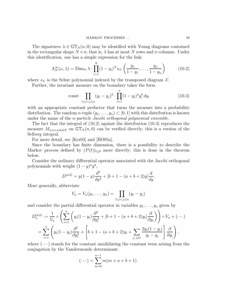
MARKOV PROCESSES . . . 59
The signatures λ ∈ GTN(n, 0) may be identified with Young diagrams containedin the rectangular shape N×n; that is, λ has at most N rows and n columns. Underthis identification, one has a simple expression for the link:
Λ∞N (ω, λ) = DimN λ ·
N∏
i=1
(1− yi)Nsλ′
(y1
1− y1, . . . ,
yn1− yn
)(10.2)
where sλ′ is the Schur polynomial indexed by the transposed diagram λ′.Further, the invariant measure on the boundary takes the form
const ·∏
1≤i<j≤n
(yi − yj)2 ·
n∏
i=1
(1− yi)aybi dyi (10.3)
with an appropriate constant prefactor that turns the measure into a probabilitydistribution. The random n-tuple (y1, . . . , yn) ⊂ [0, 1] with this distribution is knownunder the name of the n-particle Jacobi orthogonal polynomial ensemble.
The fact that the integral of (10.2) against the distribution (10.3) reproduces themeasure Mn,n+a,0,b|N on GTN (n, 0) can be verified directly; this is a version of theSelberg integral.
For more detail, see [Ker03] and [BO05a].Since the boundary has finite dimension, there is a possibility to describe the
Markov process defined by (P (t))t≥0 more directly; this is done in the theorembelow.
Consider the ordinary differential operator associated with the Jacobi orthogonalpolynomials with weight (1− y)ayb,
D(a,b) = y(1− y)d2
dy2+ [b+ 1− (a+ b+ 2)y]
d
dy.
More generally, abbreviate
Vn = Vn(y1, . . . , yn) =∏
1≤i<j≤n
(yi − yj)
and consider the partial differential operator in variables y1, . . . , yn given by
D(a,b)n :=
1
Vn
(n∑
i=1
(yi(1− yi)
∂2
∂y2i+ [b+ 1− (a + b+ 2)yi]
∂
∂yi
)) Vn + (· · · )
=
n∑
i=1
(yi(1− yi)
∂2
∂y2i+
[b+ 1− (a+ b+ 2)yi +
∑
j: j 6=i
2yi(1− yi)
yi − yj
]∂
∂yi
),
where (· · · ) stands for the constant annihilating the constant term arising from theconjugation by the Vandermonde determinant:
(· · · ) =n−1∑
m=0
m(m+ a + b+ 1).

60 ALEXEI BORODIN AND GRIGORI OLSHANSKI
Although the coefficients in front of the first order derivatives have singularities onthe hyperplanes yi = yj, the operator is well defined on smooth symmetric functionsin variables y1, . . . , yn, and it preserves this space. It also preserves the space ofsymmetric polynomials.
Theorem 10.1. Let z = n, z′ = n + a, w = 0, w′ = b, where a, b > −1. Lety1 = β+
1 , . . . , yn = β+n be the coordinates on the boundary Ω(n, 0) of the truncated
graph GT(n, 0), and recall that 1 ≥ y1 ≥ · · · ≥ yn ≥ 0.The Markov process on the simplex Ω(n, 0) determined by the Markov semigroup
(P (t))t≥0 is a diffusion whose infinitesimal generator is the differential operator
D(a,b)n with an appropriate domain containing the space of all symmetric polynomials
in variables y1, . . . , yn.
As shown in [Gor09], the same diffusion process also arises in a scaling limittransition from some discrete time Markov chains on the sets GTN(n, 0), as N →∞.
The above description of the infinitesimal generator remains true in the generalcase (10.1) of the degenerate series parameters. The only change concerns the cor-respondence between the β±-coordinates and the y-coordinates; now it takes theform
(y1, . . . , yn) = (1− β−l , . . . , 1− β−
1 , β+1 , . . . , β
+k ), n := k + l.
10.2. The formal generator. A natural question is how to extend the explicit de-scription of the infinitesimal generator obtained in Theorem 10.1 to the case of gen-eral (admissible) values of parameters (z, z′, w, w′). There are some indications thata direct generalization is impossible, in the sense that the generator cannot be ex-pressed as a second order differential operator in the natural coordinates (α±, β±, δ±)on Ω. 3 Instead of this, we present below an explicit expression for the generator ina different system of coordinates.
Introduce the functions ϕn = ϕn(ω) on Ω, n ∈ Z, as the coefficients in the Laurentexpansion of Φω(u), see (3.3) and (3.4),
Φω(u) =∑
n∈Z
ϕn(ω)un.
The functions ϕn are continuous and nonnegative on Ω, and they satisfy the relation∑
n∈Z
ϕn(ω) ≡ 1, ω ∈ Ω,
which is an immediate consequence of the fact that Φω(u) takes value 1 at u = 1 forall ω ∈ Ω.
Let us extend this definition by setting, for any N = 1, 2, . . . and any signatureν ∈ GTN ,
ϕν(ω) = det[ϕνi−i+j(ω)
]Ni,j=1
, ω ∈ Ω.
3A possible explanation is that these coordinate functions are not in the domain of the generator.

MARKOV PROCESSES . . . 61
For instance, for N = 2 we have ν = (ν1, ν2) and
ϕ(ν1,ν2) =
∣∣∣∣ϕν1 ϕν1+1
ϕν2−1 ϕν2
∣∣∣∣ = ϕν1ϕν2 − ϕν1+1ϕν2−1.
The functions ϕν appear in the expansion
N∏
i=1
Φω(ui) =∑
ν∈GTN
ϕν(ω)sν(u1, . . . , uN).
Their fundamental role is explained by (3.2).By definition, the functions ϕν are contained in the algebra of functions generated
by the functions ϕn, n ∈ Z. Conversely, any monomial in ϕn’s of degree N can beexpanded into a series on the functions ϕν , ν ∈ GTN . Namely, for arbitrary integersn1, . . . , nN , one has
ϕn1 . . . ϕnN=∑
ν∈GTN
K(ν | n1, . . . , nN)ϕν ,
where the numbers K(. . . ) are defined as the “rational” analogs of the Kostka num-bers, that is, these are the coefficients in the Laurent expansion of the rational Schurfunctions,
sν(u1, . . . , uN) =∑
n1,...,nN∈Z
K(ν | n1, . . . , nN)un11 . . . unN
N .
For instance, for N = 2 and ν = (ν1, ν2) we have
K(ν1, ν2 | n1, n2) =
1, if n1 + n2 = ν1 + ν2 and |n1 − n2| ≤ ν1 − ν2,
0, otherwise,
which implies
ϕn1ϕn2 =
∞∑
p=0
ϕ(n1+p,n2−p).
Definition 10.2. Fix an arbitrary quadruple (z, z′, w, w′) of complex parametersand introduce the following formal differential operator in countably many variablesϕn : n ∈ Z
D =∑
n∈Z
Ann∂2
∂ϕ2n
+ 2∑
n1,n2∈Zn1>n2
An1n2
∂2
∂ϕn1∂ϕn2
+∑
n∈Z
Bn∂
∂ϕn,

62 ALEXEI BORODIN AND GRIGORI OLSHANSKI
where, for any indices n1 ≥ n2,
An1n2 =
∞∑
p=0
(n1 − n2 + 2p+ 1)(ϕn1+p+1ϕn2−p + ϕn1+pϕn2−p−1)
−(n1 − n2)ϕn1ϕn2 − 2
∞∑
p=1
(n1 − n2 + 2p)ϕn1+pϕn2−p
and, for any n ∈ Z,
Bn = (n+ w + 1)(n+ w′ + 1)ϕn+1 + (n− z − 1)(n− z′ − 1)ϕn−1
−((n− z)(n− z′) + (n+ w)(n+ w′)
)ϕn.
Note that only coefficients Bn depend on the parameters (z, z′, w, w′).Assume now that the quadruple (z, z′, w, w′) satisfies the condition (6.1). As
above, let PN(t) (N = 1, 2, . . . ) and P (t) be the corresponding Markov semigroupsand let AN and A stand for their infinitesimal generators. These are densely definedoperators in the Banach spaces C0(GTN) and C0(Ω), respectively. We know thatall finitely supported functions on GTN belong to the domain of AN . This implies,cf. (3.2), that all the functions ϕν lie in the domain of A.
Theorem 10.3. Let A be the infinitesimal generator of the Markov semigroup(P (t))t≥0 with parameters (z, z′, w, w′) satisfying condition (6.1), and D be the for-mal differential operator introduced in Definition 10.2. Regard D as an operatorfrom the space C[ϕn : n ∈ Z] of polynomials in countably many variables ϕn, n ∈ Z,to the larger space C[[ϕn : n ∈ Z]] of formal series in the same variables.
Then for any N = 1, 2, . . . and any ν ∈ GTN one has
Dϕν = Aϕν .
Moreover, D is the only formal second order differential operator in variables ϕn,n ∈ Z, with such a property.
Note some properties of D:1. Formal application of D to the infinite series
∑n∈Z ϕn gives 0. This agrees with
the fact that the sum of this series on Ω equals 1 and the fact that A1 = 0.2. For any fixed integerm, D is invariant under the change of variables ϕn → ϕn+m
(n ∈ Z) combined with the shift of parameters
z → z +m, z′ → z′ +m, w → w −m, w′ → w −m,
cf. Remark 3.7 in [BO05a].3. Set z = k and w = l, where (k, l) is a couple of nonnegative integers not equal
to (0, 0). Then D respects the relations
· · · = ϕ−l−2 = ϕ−l−1 = 0 = ϕk+1 = ϕk+2 = . . .

MARKOV PROCESSES . . . 63
and thus can be reduced to an operator in the polynomial algebra C[ϕ−l, . . . , ϕk].More precisely, this means the following assertion: When D is applied to a monomialcontaining at least one variable ϕn with index n outside [−l, k] then all monomi-als entering the resulting series with nonzero coefficients have the same property.Indeed, this follows from the structure of the coefficients An1n2 and Bn.
Moreover, the resulting operator in the algebra C[ϕ−l, . . . , ϕk] can be further re-duced modulo the relation ∑
−l≤n≤k
ϕn = 1,
and then it coincides with the differential operator D(a,b)k+l from Theorem 10.1, where
a = z′ − k, b = w′ − l. Here we use the fact that quotient algebra
C[ϕ−l, . . . , ϕk]/(ϕ−l + · · ·+ ϕk = 1)
can be identified with the algebra of polynomial functions on the simplex Ω(k, l).
References
[And91] W. J. Anderson, Continuous time Markov chains: An applications-oriented approach.Springer, 1991.
[Ask87] R. Askey, An integral of Ramanujan and orthogonal polynomials . J. Indian Math. Soc.51 (1987), 27–36.
[Bor10+] A. Borodin, Schur dynamics of the Schur processes . arXiv:1001.3442[BD02] A. Borodin and P. Deift, Fredholm determinants, Jimbo-Miwa-Ueno τ-functions,
and representation theory. Comm. Pure Appl. Math. 55 (2002), 1160–1230;arXiv:math/0111007.
[BF08] A. Borodin and P. L. Ferrari, Large time asymptotics of growth models on space-like
paths I: PushASEP . Electron. J. Probab. 13 (2008), 1380–1418; arXiv:0707.2813[BF08+] A. Borodin and P. L. Ferrari, Anisotropic growth of random surfaces in 2+1 dimensions .
To appear; arXiv:0804.3035.[BG09] A. Borodin and V. Gorin, Shuffling algorithm for boxed plane partitions . Adv. Math.
220 (2009), 1739–1770; arXiv:0804.3071.[BGR09+] A. Borodin, V. Gorin, and E. M. Rains, q-Distributions on boxed plane partitions .
Selecta Math., to appear; arXiv:0905.0679.[BK10] A. Borodin and J. Kuan, Random surface growth with a wall and Plancherel measures
for O(∞), Commun. Pure Appl. Math. 63 (2010), 831–894; arXiv:0904.2607.[BO05a] A. Borodin and G. Olshanski, Harmonic analysis on the infinite-dimensional uni-
tary group and determinantal point processes . Ann. Math. 161 (2005), 1–104;arXiv:math/0109194.
[BO05b] A. Borodin and G. Olshanski, Representation theory and random point processes .In: European Congress of Mathematics, Eur. Math. Soc., Zurich, 2005, pp. 73–94;arXiv:math/0409333.
[BO05c] A. Borodin and G. Olshanski, Random partitions and the Gamma kernel . Adv. Math.194 (2005),141–202; arXiv:math-ph/0305043.
[BO06a] A. Borodin and G. Olshanski, Markov processes on partitions . Probab. Theory Rel.Fields 135 (2006), 84–152; arXiv:math-ph/0409075.

64 ALEXEI BORODIN AND GRIGORI OLSHANSKI
[BO06b] A. Borodin and G. Olshanski, Stochastic dynamics related to Plancherel measure on par-
titions . In: Representation Theory, Dynamical Systems, and Asymptotic Combinatorics(V. Kaimanovich and A. Lodkin, eds). Amer. Math. Soc. Translations, Series 2: Ad-vances in the Mathematical Sciences, vol. 217, 2006, pp. 9–21; arXiv:math-ph/0402064.
[BO09] A. Borodin and G. Olshanski, Infinite-dimensional diffusions as limits of random walks
on partitions . Probab. Theory Rel. Fields 144 (2009), 281–318; arXiv:0706.1034.[DF90] P. Diaconis and J. A. Fill, Strong stationary times via a new form of duality. Ann.
Probab. 18 (1990), 1483–1522.[EK86] S. N. Ethier and T. G. Kurtz, Markov processes — Characterization and convergence.
Wiley–Interscience, New York 1986.[Fel40] W. Feller, On the integro-differential equations of purely discontinuous Markoff processes
Trans. Amer. Math. Soc., 48 (1940), 488–815 and Errata, 58 (1945) p. 474.[Fel57] W. Feller, On boundaries and lateral conditions for the Kolmogorov differential equations .
Ann. Math. 65 (1957), 527–570.[Fel59] W. Feller, The birth and death processes as diffusion processes . J. Math. Pures Appl. 38
(1959), 301–345.[Gor09] V. Gorin, Noncolliding Jacobi processes as limits of Markov chains on the Gelfand-
Tsetlin graph. J. Math. Sciences (New York) 158 (2009), no. 6, 819–837 (translated fromZapiski Nauchnykh Seminarov POMI, Vol. 360 (2008), pp. 91123); arXiv:0812.3146.
[Ito06] K. Ito, Essentials of stochastic processes . Translated from the 1957 Japanese original.Translations of Mathematical Monographs, 231. American Mathematical Society, Prov-idence, RI, 2006.
[JM81] M. Jimbo and T. Miwa, Monodromy preserving deformation of linear ordinary differen-
tial equations with rational coefficients. II . Phys. D 2 (1981), no. 3, 407–448.[KM59] S. Karlin and J. McGregor, Coincidence probabilities . Pacific J. Math. 9 (1959), 1141–
1164.[Kat80] T. Kato, Perturbation theory of linear operators , 2nd ed. Springer-Verlag, New York,
1980.[KT09] M. Katori and H. Tanemura, Zeros of Airy function and relaxation process . J. Stat.
Phys. 136 (2009) 1177–1204; arXiv:0906.3666.[KT10] M. Katori and H. Tanemura, Non-equilibrium dynamics of Dyson’s model with an infinite
number of particles . Commun. Math. Phys. 293 (2010), 469–497; arXiv:0812.4108.[Kel83] F. P. Kelly, Invariant measures and the Q-matrix . In: Probability, statistics and analysis,
London Math. Soc. Lecture Note Ser., 79, Cambridge Univ. Press, Cambridge-New York,1983, pp. 143–160s.
[Ker03] S. V. Kerov, Asymptotic representation theory of the symmetric group and its applica-
tions in analysis . Amer. Math. Soc., Providence, RI, 2003.[KLS10] R. Koekoek, P. A. Lesky, and R. F. Swarttouw, Hypergeometric orthogonal polynomials
and Their q-analogues . Springer, 2010.[Kon05] W. Konig, Orthogonal polynomial ensembles in probability theory. Probab. Surveys 2
(2005), 385–447.[Les97] P. A. Lesky, Unendliche und endliche Orthogonalsysteme von continuous Hahnpoly-
nomen. Results Math. 31 (1997), 127–135.[Les98] P. A. Lesky, Eine Charakterisierung der kontinuierlichen und diskreten klassischen Or-
thogonalpolynome. Preprint 9812, Mathematisches Institut A, Universitat Stuttgart.[Lig99] T. Liggett, Stochastic interacting systems: contact, voter and exclusion processes .
Grundlehren der Mathematischen Wissenschaften 324. Springer-Verlag, Berlin, 1999.[Lis09+] O. Lisovyy, Dysons constant for the hypergeometric kernel . arXiv:0910.1914.
MARKOV PROCESSES . . . 65
[Macd95] I. G. Macdonald, Symmetric functions and Hall polynomials . 2nd edition. Oxford Uni-versity Press, 1995.
[Mack57] G. W. Mackey, Borel structures on groups and their duals . Trans. Amer. Math. Soc. 85(1957), 134–165.
[Mey66] P.-A. Meyer, Probability and potentials . Blaisdell, 1966.[Nor10] E. Nordenstam, On the shuffling algorithm for domino tilings . Electron. J. Probab. bf15
(2010), no. 3, 75–95; arXiv:0802.2592.[OO97] A. Okounkov and G. Olshanski, Shifted Schur functions . Algebra i Analiz 9 (1997), no. 2,
73–146 (Russian); English translation: St. Petersburg Math. J. 9 (1998), no. 2, 239–300;arXiv:q-alg/9605042.
[OO98] A. Okounkov and G. Olshanski, Asymptotics of Jack polynomials as the number of vari-
ables goes to infinity. Intern. Math. Res. Notices 1998 (1998), no. 13, 641–682; arXiv:q-alg/9709011.
[Ols03] G. Olshanski, The problem of harmonic analysis on the infinite-dimensional unitary
group. J. Funct. Anal. 205 (2003), 464–524; arXiv:math/0109193.[Ols10] G. Olshanski, Anisotropic Young diagrams and infinite-dimensional diffusion processes
with the Jack parameter . Intern. Math. Res. Notices 2010 (2010), no. 6, 1102–1166;arXiv:0902.3395.
[Ols10+] G. Olshanski, Laguerre and Meixner symmetric functions, and infinite-dimensional dif-
fusion processes . arXiv:1009.????.[Osa09+] H. Osada, Interacting Brownian motions in infinite dimensions with logarithmic inter-
action potentials . arXiv:0902.3561.[Pru63] W. E. Pruitt, Bilateral birth and death processes . Trans. Amer. Math. Soc. 107 (1963),
508–525.[Spi70] F. Spitzer, Interaction of Markov processes . Adv. Math. 5 (1970), 246–290.[Spo87] H. Spohn, Interacting Brownian particles: a study of Dyson’s model . In: Hydrodynamic
Behavior and Interacting Particle Systems, Papanicolaou, G. (ed), IMA Volumes inMathematics and its Applications, 9, Berlin: Springer-Verlag, 1987, pp. 151–179.
[VK81] A. M. Vershik and S. V. Kerov, Asymptotic theory of characters of the symmetric group.Funct. Anal. Appl. 15 (1981), 246–255.
[VK82] A. M. Vershik and S. V. Kerov, Characters and factor-representations of the infinite
unitary group. Dokl. Akad. Nauk SSSR 267 (1982), no. 2, 272–276 (Russian); Englishtranslation: Soviet Math. Dokl. 26 (1982), no. 3, 570–574 (1983).
[Voi76] D. Voiculescu, Representations factorielles de type II1 de U(∞). J. Math. Pures Appl.55 (1976), 1–20.
[War07] J. Warren, Dyson’s Brownian motions, intertwining and interlacing. Electron. J. Probab.12 (2007), 573–590; arXiv:math/0509720.
[Wey39] H. Weyl, The classical groups. Their invariants and representations . Princeton Univ.Press, 1939; 1997 (fifth edition).
[Yan90] Xiangqun Yang, The construction theory of denumerable Markov processes . Hunan Sci-ence and Technology Publ. House, 1990 (Wiley series in probability and mathematicalstatistics : Probability and mathematical statistics).
[Zhe70] D. P. Zhelobenko, Compact Lie groups and their representations , Nauka, Moscow, 1970(Russian); English translation: Transl. Math. Monographs 40, Amer. Math. Soc., Prov-idence, RI, 1973.

66 ALEXEI BORODIN AND GRIGORI OLSHANSKI
California Institute of Technology; Massachusetts Institute of Technology;
Institute for Information Transmission Problems, Russian Academy of Sciences
E-mail address : [email protected]
Institute for Information Transmission Problems, Bolshoy Karetny 19, Moscow
127994, Russia; Independent University of Moscow, Russia
E-mail address : [email protected]