www.oeaw.ac.at

www.ricam.oeaw.ac.at

Markov Chain Monte CarloMethods for Parameter

Estimation inMultidimensional Continuous

Time Markov SwitchingModels

M. Hahn, S. Frühwirth-Schnatter, J. Sass

RICAM-Report 2007-09

Markov Chain Monte Carlo Methods for Parameter

Estimation in Multidimensional Continuous Time

Markov Switching Models∗

Markus Hahn†, Sylvia Fruhwirth-Schnatter‡, Jorn Sass†

April 5, 2007

Abstract

We present Markov chain Monte Carlo methods for estimating pa-rameters of multidimensional, continuous time Markov switching mod-els. The observation process can be seen as a diffusion, where driftand volatility coefficients are modeled as continuous time, finite stateMarkov chains with a common state process. The states for drift andvolatility and the rate matrix of the underlying Markov chain haveto be estimated. Applications to simulated data indicate that theproposed algorithm can outperform the expectation maximization al-gorithm for difficult cases, e.g. for high rates. Application to financialmarket data shows that the Markov chain Monte Carlo method indeedprovides sufficiently stable estimates.

Keywords: Bayesian inference, data augmentation, hidden Markovmodel, switching diffusion

JEL classification codes: C11, C13, C15, C32

1 Introduction

Typical dynamics of a price process S = (St)t∈[0,T ] of n stocks are

dSt = Diag(St)(µt dt+ σt dWt), S0 = s0, (1)

where Diag(St) denotes the diagonal matrix with diagonal St = (S1t , . . . , S

nt ).

Here W = (Wt)t∈[0,T ] is an n-dimensional Brownian motion, s0 is the initialprice vector, µ = (µt)t∈[0,T ] the drift process, σ = (σt)t∈[0,T ] the volatility

∗An updated version of this paper has appeared in the IFAS research paper series asno. 2009-41 and is available for download at http://www.ifas.jku.at

†Johann Radon Institute for Computational and Applied Mathematics, AustrianAcademy of Sciences, Linz, Austria

‡Department for Applied Statistics and Econometrics, University Linz, Austria

1

process and T > 0 the terminal trading time. Suppose that µ and σ cantake d possible values and that switching between these values is governedby a state process Y which is a continuous time Markov chain with statespace 1, . . . , d and rate matrix Q. Then the corresponding return processR = (Rt)t∈[0,T ], defined by dRt = (Diag(St))−1 dSt, satisfies

dRt = µt dt+ σt dWt (2)

and represents a continuous time Markov switching model (MSM). In caseof constant σ we call it a hidden Markov model (HMM). For a MSM incontinuous time, in principle the state process Y can be observed via thequadratic variation of R. This is not possible for a HMM, Y is hidden.

Continuous time MSMs (e.g. Buffington and Elliott (2002), Guo (2001)),discrete time MSMs (e.g. Engel and Hamilton (1990)), and discrete as wellas continuous time HMMs (e.g. Liechty and Roberts (2001), Sass and Hauss-mann (2004)) are widely used in finance, but are also applied in many otherareas such as in biophysics (e.g. Rosales et al. (2001), Ball et al. (1999)).

In the present paper, we consider joint modeling of several stock pricesusing MSMs. Although stock prices are observed only in discrete time, like inmany other inference problems encountered in finance, it is more convenientto use continuous time models since these allow the derivation of closed formsolutions. For example, Sass and Haussmann (2004) derive explicit optimaltrading strategies for a portfolio optimization problem based on a continuoustime HMM. The practical application of these strategies, however, requiresknown values for the parameters of the continuous time stock model, andone faces the problem of estimating parameters of a continuous time modelfrom discrete observations. Since in continuous time S and R generate thesame filtration, we can assume that we observe R, hence we have to estimateparameters of a MSM like (2), or a HMM, if σ is constant.

One might use a moment based method, see e.g. Elliott et al. (2006),which yields good estimates, provided that the number of observations isvery large (depending on the noise level, they present results for 10 000to 20 000 observations for simulated data and 30 000 to 150 000 for marketdata).

In discrete time the expectation maximization (EM) algorithm (Demp-ster et al. (1977)) can be used to estimate the drift and covariance coeffi-cients as well as the rate matrix governing the switching of the states, seee.g. Elliott et al. (1997) or Engel and Hamilton (1990). For low rates andlow volatility the EM algorithm provides very accurate results, but esti-mation results in Sass and Haussmann (2004) indicate that for high rates,where a jump occurs between two observations with high probability, theEM algorithm performs poorly. For a continuous time HMM one can use acontinuous time version of the EM algorithm as presented in James et al.(1996). For a continuous time MSM, however, no finite-dimensional filters

2

are known, making it impossible to employ the EM algorithm to estimatethe volatility jointly with the other parameters since the change of measureinvolved in deriving the filters used in the EM algorithm requires known σ(cf. Elliott et al. (1995)).

In this paper, we consider a Bayesian approach to parameter estimation,using Markov chain Monte Carlo (MCMC) methods, which is capable ofdealing both with continuous time HMMs as well as continuous time MSMs.A Bayesian approach has been considered, for instance, by Rosales et al.(2001) and Boys et al. (2000) for discrete time HMMs, Ball et al. (1999)and Liechty and Roberts (2001) for continuous time HMMs, and Kim andNelson (1999) for discrete time MSMs, dealing with problems in biophysics,bioinformatics and economics.

It is the aim of this paper to extend these methods to multidimensionalcontinuous time HMMs and MSMs. We are particularly interested to esti-mate parameters in a multidimensional MSM with high rates, considerablenoise, based on not too many observations (less than, say, 5000), as this isthe typical situation one faces for many financial time series. We assume,however, that the number of states is given, and refer to Otranto and Gallo(2002) and Fruhwirth-Schnatter (2006, Chapter 4 and 5) for the matter ofmodel selection. As comparisons between the discrete and continuous mod-els seem to be hardly treated in the relevant literature, we treat both thecase of a discrete time approximation as well as methods for continuous time.We develop a Metropolis-Hastings sampler employing data augmentation byadding the state process to the unknowns. Hence, for the update of the ratematrix a Gibbs step can be used. In the discrete case, a Gibbs step is usedalso for the state process update, while in continuous time proposing thestate process conditioning only on the rate matrix is much faster.

In Section 2, the stock return model which is a continuous time mul-tidimensional MSM is introduced in more detail. In Section 3, MCMCestimation for continuous time state processes (referred to as CMCMC) isdescribed. In Section 4, we present the approximating discrete time modeland the corresponding MCMC algorithm (referred to as DMCMC). For bothalgorithms, we give the a priori and conditional distributions and describethe proposals and sampling methods used. We deal with the approximationerror and the problem of computing the rate matrix corresponding to a tran-sition matrix. In Section 5, we deal with issues concerning the applicationof the methods presented in Sections 3 and 4. Finally, we show numericalresults for simulated as well as market data from daily stock index quotes.

2 Continuous Time Markov Switching Model

In this section we present the market model which is a multidimensionalcontinuous time MSM. On a filtered probability space (Ω,F = (Ft)t∈[0,T ],P)

3

we observe in [0, T ] the n-dimensional process R = (Rt)t∈[0,T ],

Rt =∫ t

0µs ds+

∫ t

0σs dWs, (3)

where W = (Wt)t∈[0,T ] is an n-dimensional Brownian motion with respectto F . The drift process µ = (µt)t∈[0,T ] and the volatility process σ =(σt)t∈[0,T ], taking values in Rn and Rn×n, respectively, are continuous time,time homogeneous, irreducible Markov processes with d states, adapted to Fand independent of W , driven by the same state process Y = (Yt)t∈[0,T ].We denote the possible values of µ and σ by B = (µ(1), . . . , µ(d)) andΣ = (σ(1), . . . , σ(d)), respectively. We assume the volatility matrices σ(k)

to be nonsingular and use the notation C(k) = σ(k) (σ(k))>. Sometimes wewill interpret B as a matrix, i.e. Bik = µ

(k)i . The state process Y , which is a

continuous time, time homogeneous, irreducible Markov chain adapted to F ,independent of W , with state space 1, . . . , d, allows for the representations

µt = µ(Yt) =d∑

k=1

µ(k) IYt=k, σt = σ(Yt) =d∑

k=1

σ(k) IYt=k. (4)

The state process Y is characterized by the rate matrix Q ∈ Rd×d asfollows: For λk = −Qkk =

∑dl=1,l 6=k Qkl, k = 1, . . . , d, in state k the waiting

time for the next jump is λk-exponentially distributed, and the probabilityof jumping to state l 6= k when leaving k is given by Qkl/λk.

Starting from a prior distribution of the unknown parameters P(Q,B,Σ)we wish to determine P(Q,B,Σ | (Vm)m=1,...,N ), the posterior distribution ofthese parameters given the observed data

Vm = ∆Rm ∆t =∫ m ∆t

(m−1) ∆tµs ds+

∫ m ∆t

(m−1) ∆tσs dWs, m = 1, . . . , N. (5)

Remark 1. One cannot distinguish between the pairs (σ,W ) and (σ, W ),where σ is a square-root of σσ> and W = σ−1σW . However, without loss ofgenerality we can assume σ(k) to be a lower triangular matrix, i.e. σ(k)(σ(k))>

equals the Cholesky factorization of the covariance matrix.

3 MCMC for Continuous Time State Process

In this section, we describe an MCMC algorithm for the continuous timemodel (referred to as CMCMC) to estimate the parameters Q, B and Σgiven stock returns, V = (Vm)m=1,...,N , observed at fixed observation times∆t, 2∆t, . . . , N ∆t = T . This method is easily extended to deal with non-equidistant observations, see Remark 3 below. We allow for jumps of thehidden state process at any time and especially for any number of jumpswithin each observation interval.

4

3.1 Data Augmentation

The state process Y , which is allowed to jump any time, is described bythe process of jump times, J = (Jh)h=0,...,H , and the sequence of statesvisited, Z = (Zh)h=0,...,H , where H is the number of jumps of Y in [0, T ],i.e. J0 = 0 and Z0 = Y0, Jh is the time of the h-th jump, and Zh is the stateY jumps to at the h-th jump. Hence the inter-arrival time ∆Jh = Jh−Jh−1

is exponentially distributed with parameter λZh−1. Notice that Jh+1 and

Zh+1 are independent given Jh and Zh.For parameter estimation, we augment the parameter space by adding

the state process Y , and determine the joint posterior distribution of Q, B,Σ, and Y given the observed data V .

3.2 Prior Distributions

Prior distributions have to be chosen for Q, B, Σ, and Y0. We consider twoprior specifications, differing in the prior assumptions concerning the initialstate Y0. The first prior is based on assuming prior independence among allparameters.

Assumption 1. Q, B, Σ, and Y0 are a priori independent, i.e.

P(Q,B,Σ, Y0) = P(Q) P(B) P(Σ) P(Y0). (6)

Further, for i = 1, . . . , n, k, l = 1, . . . , d, l 6= k,

Qkl ∼ Γ(fkl, gkl),

µ(k)i ∼ N(mik, s

2ik),

C(k) ∼ IW(Ξ(k), νk),Y0 ∼ U(1, . . . , d).

(7)

Also, the off-diagonal elements of Q are independent. With Γ, N, IW, and Uwe refer to the Gamma, normal, inverted Wishart, and uniform distribution,respectively.

Remark 2. For the inverted Wishart distribution, we use the parametriza-tion where the density is given through

fIW(C; Ξ, ν) ∝ (detC)−ν−(n+1)/2 exp(− tr(ΞC−1)

)(8)

and the expected value is given as E[C] = Ξ (ν − (n+ 1)/2)−1.

If we think of time 0 as the beginning of our observations after theprocess has already run for some time, it may be reasonable to alter theprior distribution as follows:

5

Assumption 1a. Q and Y0 are a priori dependent:

P(Q,B,Σ, Y0) = P(Q) P(Y0 |Q) P(B) P(Σ), (9)

and the state process starts from its ergodic probability ω, i.e. P(Y0 |Q) = ω.All other prior assumptions are the same as in Assumption 1.

Under the second assumption, Y given Q is a stationary Markov chain,i.e. P(Yt |Q) = ω for all t ∈ [0, T ].

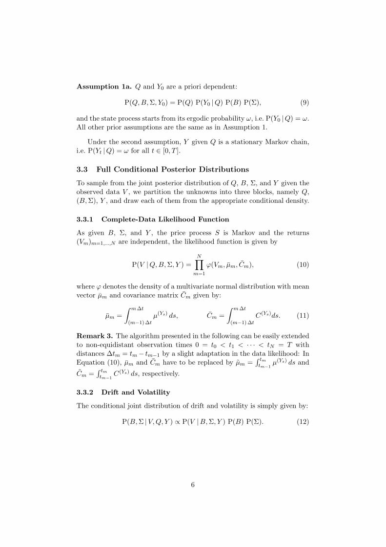
3.3 Full Conditional Posterior Distributions

To sample from the joint posterior distribution of Q, B, Σ, and Y given theobserved data V , we partition the unknowns into three blocks, namely Q,(B,Σ), Y , and draw each of them from the appropriate conditional density.

3.3.1 Complete-Data Likelihood Function

As given B, Σ, and Y , the price process S is Markov and the returns(Vm)m=1,...,N are independent, the likelihood function is given by

P(V |Q,B,Σ, Y ) =N∏

m=1

ϕ(Vm, µm, Cm), (10)

where ϕ denotes the density of a multivariate normal distribution with meanvector µm and covariance matrix Cm given by:

µm =∫ m ∆t

(m−1) ∆tµ(Ys) ds, Cm =

∫ m ∆t

(m−1) ∆tC(Ys)ds. (11)

Remark 3. The algorithm presented in the following can be easily extendedto non-equidistant observation times 0 = t0 < t1 < · · · < tN = T withdistances ∆tm = tm− tm−1 by a slight adaptation in the data likelihood: InEquation (10), µm and Cm have to be replaced by µm =

∫ tmtm−1

µ(Ys) ds and

Cm =∫ tmtm−1

C(Ys) ds, respectively.

3.3.2 Drift and Volatility

The conditional joint distribution of drift and volatility is simply given by:

P(B,Σ |V,Q, Y ) ∝ P(V |B,Σ, Y ) P(B) P(Σ). (12)

6

3.3.3 State Process

The prior distribution of the state process Yt for t ∈ ]0, T ] is determined bythe distribution of Y0 and the rate matrix Q, and is independent of B and Σ.Therefore we obtain the following full conditional posterior:

P(Y |V,Q,B,Σ) ∝ P(V |B,Σ, Y ) P(Y |Q). (13)

The probability of Y given Q equals (cf. Ball et al. (1999))

P(Y |Q) = P(Y0 |Q)H∏

h=1

(λZh−1

e−λZh−1∆Jh

QZh−1,Zh

λZh−1

)e−λZH

(T−JH) (14)

= P(Y0 |Q)d∏

k=1

d∏l=1l 6=k

(e−Qkl Ok

T QNklkl

), (15)

where OkT denotes the occupation time of state k, and Nkl denotes the

number of jumps from state k to l,

OkT =

∫ T

0IYt=k dt, Nkl =

H∑h=1

IZh−1=k,Zh=l. (16)

3.3.4 Rate Matrix

Using (15) and the independence of the priors of Qkl, we have

P(Q |V,B,Σ, Y ) ∝ P(Y0 |Q)d∏

k=1

d∏l=1l 6=k

ψkl(Qkl) (17)

(cf. Ball et al. (1999)), where ψkl is a Gamma distribution with parametersfkl + Nkl and gkl + Ok

T . If Y0 is independent of Q, we can drop the termP(Y0 |Q) and the off-diagonal elements Qkl, k 6= l, are Gamma distributed.

3.4 Proposal Distributions

3.4.1 Drift and Volatility

For the update of B and Σ, a joint normal random walk proposal, reflectedat 0 for the diagonal entries of σ(k), is used:

B′ = B + rB φ, σ(k)ij

′= σ

(k)ij + rσ ψ

(k)ij , σ

(k)ii

′=

∣∣σ(k)ii + rσ ψ

(k)ii

∣∣, (18)

where φ and ψ are n×d and n×n matrices of independent standard normalvariates, i = 1, . . . , n, j = 1, . . . , i − 1, k = 1, . . . , d, and rB and rσ areparameters scaling the step widths.

7

As the transition kernel is symmetric, we have a Metropolis step withacceptance probability αB,Σ = min1, αB,Σ, where:

αB,Σ =P(V |B′,Σ′, Y ) P(B′) P(Σ′)P(V |B,Σ, Y ) P(B) P(Σ)

. (19)

Remark 4. The update of σ rather than C = σσ> guarantees that theresulting covariance matrix is positive semi-definite, as a symmetric matrixis positive definite if and only if there is a Cholesky decomposition: Forevery non-null vector v we have v>Cv = v>σσ>v = (σ>v)>(σ>v) ≥ 0; if σis non-singular, then C is positive definite.

Remark 5. A common problem that occurs in Bayesian methods for theanalysis of Markov switching models is label switching (for a detailed dis-cussion see e.g. Fruhwirth-Schnatter (2006, Section 3.5)). Although due tothe prior distribution (7) the posterior is not invariant to relabeling in ourcase, it is more effective to constrain the parameter space appropriately.

This can be done by proposing only values for B′ that keep up a certainorder, e.g. for n = 1 we can simply demand that B′

11 > ... > B′1d. Con-

straints for the multidimensional case can be introduced as follows. If weassume that the drift for each asset return Ri can take di different valuesblii , li = 1, . . . , di, we set the total number of states to be d =

∏ni=1 di. Then

B = (µ(1), . . . , µ(d)) consists of all possible vectors (bl11 , . . . , blnn )>, where

li ∈ 1, . . . , di for i ∈ 1, . . . , n. The drift vectors µ(k), k = 1, . . . , d,can be sorted e.g. in lexicographical order, so µ(1) = (b11, . . . , b

1n)> contains

the highest and µ(d) = (bd11 , . . . , b

dnn )> contains the lowest drift for each as-

set. This ordering can be easily maintained in each update, guaranteeing aunique labeling.

Even with constraints on the parameter space, label switching can stillconstitute a problem (cf. Stephens (2000)). In our examples, we never en-countered such problems. However, if the posterior densities show evidenceof label switching like multi-modality, methods like relabeling (Stephens(2000), Celeux (1998)), random permutation (Fruhwirth-Schnatter (2001b)and Fruhwirth-Schnatter (2001a)), or the use of invariant loss functions(Celeux et al. (2000), Hurn et al. (2003)) are necessary; a review of thesemethods is found in Jasra et al. (2005).

3.4.2 State Process

For updating the block (Yt)t∈[t0,t1[, 0 < t0 < t1 < T , we generate a proposal(Y ′

t )t∈[0,t′[, t′ = t1 − t0, as follows: First, we set Z ′0 = Yt0 . Then we simulate

the waiting time until the next jump time and the state the chain jumpsto given the rate matrix Q. This is repeated until the jump time is greaterthan t′, which is assumed to happen afterH ′+1 steps, i.e. there areH ′ jumpsin [0, t′[. In order to fit the proposal Y ′ to Y , we have to consider three cases.

8

If Z ′H′ = Yt1 we are done. If Z ′

H′ 6= Yt1 and H ′ > 0, we enforce Z ′H′ = Yt1 ,

possibly removing the last jump, if the chain was in state Yt1 before thejump. Finally, if Z ′

H′ 6= Yt1 and H ′ = 0, we just start over.So what is the probability of proposing some given Y ′? Denote the

originally proposed parameters by Y , J , Z, H, the adapted proposals byY ′, J ′, Z ′, H ′, and Y = (Yt)t∈ [t0,t1[.

First assume t0 > 0, t1 < T , and H ′ > 0. A possible adaptation ofY affects only the time interval [J ′H′ , t′[. We distinguish between the casesH ′ = H and H ′ = H − 1 to obtain

q(Y , Y ′) =H′−1∏h=1

(e−λZ′

h−1∆J ′

h QZ′h−1,Z′

h

)e−λZ′

H′−1∆J ′

H′

×( ∑

j 6=Z′H′−1

QZ′H′−1

,j e−λj(t

′−J ′H′ )

+QZ′H′−1

,Z′H′

∑j 6=Z′

H′

QZ′H′ ,j

f(λZ′H′, λj , t

′ − J ′H′)), (20)

where

f(λ1, λ2, t) =

e−λ1t−e−λ2t

λ2−λ1if λ1 6= λ2,

t e−λ1t if λ1 = λ2.

For H ′ = 0, where final and initial states coincide and H ∈ 0, 1, q takesthe simpler form

q(Y , Y ′) = e−λZ′

0t′

+∑j 6=Z′

0

QZ′0,j f(λZ′

0, λj , t

′). (21)

For updating (Yt)t∈[0,t1[, Y′0 is sampled from the initial distribution of the

state process and in (20) and (21) the factor P(Y ′0 |Q) enters.

For updating (Yt)t∈[t0,T ], no adaptations are needed, i.e. Y = Y ′; in (20)

the second line is replaced with QZ′H′−1

,Z′H′e−λZ′

H′(t′−J ′

H′ ) and in (21) thesum is dropped.

Set Y = (Yt)t∈[0,T ]\[t0,t1[ and let V denote the set of observed data fortime [t0, t1[. Then the conditional probability of the proposal restricted tothis interval is given by

P(Y ′ |V ,B,Σ, Q, Y ) =

P(V |B,Σ, Y ′)H′∏

h=1

(e−λZ′

h−1∆J ′

h QZ′h−1,Z′

h

)e−λZ′

H′(t′−J ′

H′ ). (22)

9

Combining (10), (22), and (20) (or (21)), we compute the acceptance prob-ability αY = min1, αY , where:

αY =P(V |B,Σ, Y ′)P(V |B,Σ, Y )

P(Y ′ |Q)q(Y , Y ′)

q(Y ′, Y )P(Y |Q)

.

Comparing (14) and (20), note that most terms in P(Y ′ |Q)/q(Y , Y ′) andq(Y ′, Y )/P(Y |Q) cancel. For t0 = 0, αY is replaced by α

(0)Y , while for

t1 = T , αY simplifies to α(T )Y , where

α(0)Y =

P(Y ′0 |Q)

P(Y 0 |Q)αY , α

(T )Y =

P(V |B,Σ, Y ′)P(V |B,Σ, Y )

.

3.4.3 Rate Matrix

To update the rate matrix, we sample from a Gamma distribution. Fork, l = 1, . . . , d, l 6= k, the proposal

Q′kl ∼ Γ(fkl +Nkl, gkl +Ok

T ), Q′kk = −

d∑l=1l 6=k

Q′kl (23)

is used. If the initial distribution of the state process P(Y0) is independentof Q, then (23) is already a draw from the appropriate full conditional dis-tribution, and we obtain a Metropolis-Hastings step with acceptance rate 1,i.e. a Gibbs step. Otherwise, using Assumption 1a, we accept the drawwith probability αQ = min1, αQ, where αQ equals the ratio of the ergodicprobabilities of Y0 given the new and old rate matrix, i.e.

αQ =P(Y0 |Q′)P(Y0 |Q)

=ω′

ω. (24)

4 MCMC for Discrete Time Approximation

In this section, we describe an algorithm (referred to as DMCMC) to esti-mate the parametersQ, B, and Σ given the stock returns at fixed observationtimes ∆t, 2∆t, . . . , N ∆t = T assuming that the state process jumps only atthe end of these observation times. That means that over each observationtime interval the drift of the return is constant. While this gives a goodapproximation of the continuous time model if the rates are not too high(compared to the time step ∆t), it allows a better adaption of the algorithmto the model and can lead to more stable results. Finally, we give someconsiderations for the approximation error and discuss the problem of howto compute the rate matrix corresponding to some transition matrix.

10

4.1 The Model

To allow jumps of the state process at the observation times only, we re-place the rate matrix Q by the transition matrix X ∈ Rd×d, where Xkl =P(Yt+∆t = l |Yt = k), i.e. X = exp(Q∆t). Then the probability of leavingstate k is simply 1 − Xkk and the time spent in state k is geometricallydistributed with parameter Xkk. The step process Y is fully described byits values at times m∆t, m = 0, . . . , N − 1, and the unknown state processreduces to Y = (Ym)m=0,...,N−1; the same notation is used for µ and σ.

Starting from a prior distribution of the unknown parameters P(X,B,Σ),we determine the augmented posterior distribution P(X,B,Σ, Y |V ), giventhe observed data V = (Vm)m=1,...,N , where in comparison to the previoussection, Vm simplifies to

Vm = µm−1 ∆t+ σm−1 (Wm ∆t −W(m−1) ∆t). (25)

4.2 Prior Distributions

Prior distributions have to be chosen for X, B, Σ, and Y0, and as in Subsec-tion 3.2, we consider two prior specifications, differing in the prior assump-tions concerning the initial state Y0. The independent priors are essentiallythe same as in (6), with P(Q) being substituted by P(X).

Assumption 2. X, B, Σ, and Y0 are independent, i.e.

P(X,B,Σ, Y0) = P(X) P(B) P(Σ) P(Y0), (26)

where for k = 1, . . . , d, the rows Xk· of X are assumed to be independentand to follow a Dirichlet distribution:

Xk· ∼ D(gk1, . . . , gkd). (27)

The stationary prior is essentially the same as in (9), with P(Q) P(Y0 |Q)being substituted by P(X) P(Y0 |X).

Assumption 2a. X and Y0 are a priori dependent:

P(X,B,Σ, Y0) = P(X) P(Y0 |X) P(B) P(Σ), (28)

and the state process starts from its ergodic probability ω, i.e. P(Y0 |X) = ω.P(B) and P(Σ) are the same as in Assumption 1, P(X) is the same as inAssumption 2.

4.3 Sampling from the Full Conditional Posterior Distribu-tions

To sample from the posterior, we partition the unknowns into X, (B,Σ), Y .

11

4.3.1 Complete-Data Likelihood Function

The complete-data likelihood function (10) reduces to:

P(V |X,B,Σ, Y ) =N∏

m=1

ϕ(Vm, µ(Ym−1) ∆t, C(Ym−1) ∆t), (29)

where ϕ denotes the density of a multivariate normal distribution with meanvector µ(k) and covariance matrix C(k), whenever Ym−1 = k.

4.3.2 Drift and Volatility

The conditional distribution of drift and volatility is the same as in (12).For the update of B and Σ, we proceed exactly as in the continuous case,using a joint random walk proposal. Note, however, that a more efficientGibbs update would also be available, as a joint update of all elements of Bconditional on Σ and of all elements of Σ conditional on B is feasible.

4.3.3 State Process

The prior distributions of the state process Ym, m = 1, . . . , N − 1 is deter-mined by the distribution of Y0, and the transition probabilities X, and isindependent of B and Σ. Therefore the full conditional posterior reads:

P(Y |V,B,Σ, X) ∝ P(V |B,Σ, Y ) P(Y |X). (30)

DefiningNkl =∑N−1

m=1 IYm−1=k, Ym=l, the number of transitions from state kto l, the probability of Y given X is

P(Y |X) = P(Y0 |X)N−1∏m=1

P(Ym |Ym−1, X) = P(Y0 |X)d∏

k,l=1

XNklkl . (31)

By forward-filtering-backward-sampling, see Fruhwirth-Schnatter (2006), wemay update Y drawing from the full conditional posterior P(Y |V,B,Σ, X).One such update, however, requires roughly N × d evaluations of an n-dimensional normal distribution and the generation of N discrete randomnumbers. Thus, this step (in particular, computing the filtered probabilities)is by far the most costly part of one update step. So we do not update thewhole process Y in each step, but we randomly choose a block of approx-imately exponentially distributed lengths. Fixing the average block lengthhas to be done weighing higher computation time in each step against fastermixing (compare Section 5.1).

12

4.3.4 Transition Matrix

For the update of the transition matrix, we use the method of sampling froma Dirichlet distribution as described e.g. in Fruhwirth-Schnatter (2006). Foreach row k = 1, . . . , d of the transition matrix, the proposal

X ′k ∼ D(gk1 +Nk1, . . . , gkd +Nkd), (32)

is used. If the initial distribution of the state process P(Y0) is independentof X, then X ′

k is a sample from the appropriate full conditional distribu-tion, and we obtain a Gibbs step with acceptance rate 1. Otherwise (usingAssumption 2a) we accept the draw with probability αX = min1, αX,where:

αX =P(Y0 |X ′)P(Y0 |X)

=ω′

ω. (33)

4.4 Discretization Error

The algorithm presented in this section is tailored to a discrete time model.Hence, we give some considerations about the error that arises from ignoringjumps within observation times.

The estimation of Q from a given (true) transition matrix X shouldintroduce no error: the computation of Q from X via the matrix logarithmtakes into account possible jumps occurring between the observation times.

The error in the estimated drift parameters occurs as follows: In thecontinuous model, B represents the instantaneous rates of return. If weassume Y , Q, and Σ to be known and denote the occupation time of statek in [0, t] with Ok

t , we estimate in the discrete algorithm

Bik = E[V im ∆t−1 |Ym−1 = k,Q,Σ] =

d∑l=1

Bil E[Ol

∆t

∆t

∣∣∣Y0 = k,Q]. (34)

If the rates are high compared to the observation time interval, i.e. if thenumber of expected jumps within one period gets high, Bik approaches∑d

l=1Bil ωl regardless of k, while for low rates Bik is close to Bik.Next we give a rough analysis of the covariance estimate. As Y and W

are independent, the observed covariance of the returns is the sum of thecovariances resulting from state jumps within observation intervals and theBrownian motion. As

∫ t0 µ

isds =

∑dk=1Bik O

kt , we have given Y0, Q, and B

C(k) = B Cov[O∆t |Y0 = k,Q]B> ∆t−1 +d∑

l=1

C(l) E[Ol

∆t

∆t

∣∣∣Y0 = k,Q].

(35)

However, estimating all parameters together, there is much interaction,e.g. if the drifts are underestimated, the volatility is overestimated.

13

4.5 Finding Generators for Transition Matrices

Employing DMCMC, we face the problem of computing the generator ma-trix Q corresponding to some transition matrix X for a fixed time step ∆t.The problem of the existence of an adequate rate matrix (embedding prob-lem) was already addressed by Elfving (1937) and in more detail by Kingman(1962), however, only recently the problem regained interest in the contextof credit risk modeling, see e.g. Israel et al. (2001) for a collection of theoret-ical results and Kreinin and Sidelnikova (2001) for regularization algorithmsfor the computation of an (approximating) generator. Bladt and Sørensen(2005) describe how to find maximum likelihood estimators for Q using theEM algorithm or MCMC methods.

The problem turns out to be non-trivial for matrices of dimension greaterthan two. In general, there may exist no, one or more than one matrices Qsuch that X = exp(Q∆t) and Q is a valid generator. If the transition matrixis strictly diagonally dominant, than there is at most one generator (Israelet al., 2001, Remark 2.2), that is, the matrix logarithm of X exists uniquely,but need not yield a valid generator. A result in Culver (1966) implies thesame if all eigenvalues of X are positive and distinct. If the (unique) ma-trix logarithm of X contains negative off-diagonal elements, we have to lookfor an approximating generator. Kreinin and Sidelnikova (2001) proposeto regularize such invalid generators by projecting onto the space of validgenerators. Another possibility is setting all negative off-diagonal entries,which are very small usually, to zero and adjusting all other elements pro-portional to their magnitude. Another problem occurs if there are multiplevalid generators: Israel et al. (2001) state that choosing different generatorsresults in different values Xt(Q) = exp(Qt) for most t. Then one can choosethe generator that represents the transition matrix best in some sense, seeIsrael et al. (2001, Remark 5.1), for some considerations.

However, in our application there is another possibility to avoid theseproblems by restricting the parameter space for X to all uniquely embed-dable transition matrices. This can be accomplished by rejecting and re-drawing updates for X that do not have a unique corresponding generator.

5 Applications

In this section, we describe some details on the implementation. Then wepresent numerical results of the proposed algorithms both for simulateddata and historical prices. Regarding the small number of observations andthe relatively high volatility, we cannot expect to get very accurate results(especially for the rates, which are most difficult to estimate). However, weget reasonable results that are not visible to the naked eye. In particular,our methods turn out to have some advantages over the widely used EMalgorithm.

14

5.1 Notes on the Implementation

We discuss how parameters of the prior and proposal distributions as wellas initial values can be chosen.

5.1.1 Choosing the Prior

Although, asymptotically, the hyperparameters of the prior distributionshave vanishing influence on the results, they should be chosen with care,as we are dealing with a limited number of observations, in order not tointroduce some bias or predetermine the results too strongly. Slightly datadependent priors can be used to define the prior for the drift and volatilityparameters, see, for instance, the market data example discussed in Subsec-tion 5.2.2. For the transition matrix in DMCMC, the vector gk· equals thea priori expectation of Xk· times a constant that determines the variance.If X0 denotes our prior expectation of X, we may set gk· = X0

k· ck. Then ckcan be interpreted as the number of observations for jumps out of state kin the prior distribution (added to the information contained in the data).The prior of the rate matrix for CMCMC is chosen in such a way that fkl

and gkl in (7) are equal to the prior expectation of the number of jumpsfrom k to l and the occupation time in state k, respectively, both times thesame factor. Hence, denoting the expected rate matrix by Q0, fk· is set toQ0

k· ck and gkl to ck, where the constant ck determines the variance of theprior distribution. Similar as in the discrete case, ck can be interpreted asthe time we observe state k a priori.

For simulated data hyperparameters can be chosen such that the priorexpectation equals the true values in order to avoid a bias.

5.1.2 Running MCMC

To implement the Metropolis-Hastings algorithm, the scaling factors rB andrσ have to be selected in (18). We found that selecting rB around 1 to 5 %of the minimal difference between two adjacent initial drift values workedwell whereas rσ is set to 1% of the maximal element of the initial volatilitymatrix.

When updating the state process in CMCMC, the acceptance rate tendsto be very low for proposal blocks that are too long. Hence we choose theaverage block length such that about 25 % of the proposals are accepted.Additionally, we found it useful to fix an upper bound for the block length.For the parameter determining the average and the maximal block length,suitable values were found by monitoring the acceptance in dependence onthe block length in various test runs. In our numerical experiments anaverage of about 3 % and a maximal length of 7 % of the data availableturned out to be a good choice resulting in an average acceptance about 25 %.

15

The same block length works well in DMCMC to reduce the computationalcosts of updating the whole state process.

Finally, starting from initial values for the trend, volatility, and rates(e.g. prior means), we generate an initial value for the state process bysimulating from the smoothed discrete time state estimates.

5.2 Numerical Results

For 2 assets, 4 states, and 1500 observations, about 10 000 steps per minutecan be performed with CMCMC. The discrete version is a little bit slower, asthe smoothed sampling of the states is costly. Depending on the data, 50 000up to 2 000 000 steps are needed for reliable results. Generally, the quality ofthe estimates is proportional to the difference between the drifts µ(k)

i −µ(k+1)i

and indirect proportional to the magnitude of the variances (C(k))ii and therates λk. Clearly, the more data available the better the results are; thisalso implies that estimates for parameters for states that are visited lessfrequently are less reliable and have higher variance.

5.2.1 Comparison for Simulated Data

To compare DMCMC, CMCMC, and the EM algorithm we consider 500samples of simulated prices (N = 1500, T = 6, ∆t = 1/250) with continuousstate processes and constant volatility.

For the EM algorithm we use initial values (1,−1) for the drifts of bothassets, whereas the off-diagonal elements of the initial rate matrix are setto 32. The covariances are pre-estimated using regressing for approximationsof the quadratic variation process of the return for different step widths.This method was developed in Sass and Haussmann (2004), where we alsorefer to for a detailed description of the continuous time EM algorithm usingrobust filters for HMMs based on James et al. (1996) used here. 250 stepsare sufficient for the EM algorithm to converge.

In the MCMC samplers 100 000 iterations are performed where the first25 000 values are discarded. For the MCMC algorithms we use the followinga priori distributions: For the drifts of both assets the mean values areset to (2,−2) and the standard deviations to 2. For the volatility, the flatprior p(C) ∝ c is used for C = σσ>, and we start from initial volatilityDiag(0.2, 0.2). The mean transition matrix is set to its true value, the meanrate matrix has off-diagonal entries 17.2; the standard deviations for X andQ are

0.23 0.18 0.15 0.110.15 0.22 0.15 0.110.11 0.15 0.22 0.150.11 0.15 0.18 0.23

,

0 12.9 10.0 6.9

10.6 0 10.0 6.96.9 10.0 0 10.66.9 10.0 12.9 0

, (36)

16

respectively. The state process is initialized by sampling from the smoothedstate estimates for a discrete process given the initial values for the remainingparameters.

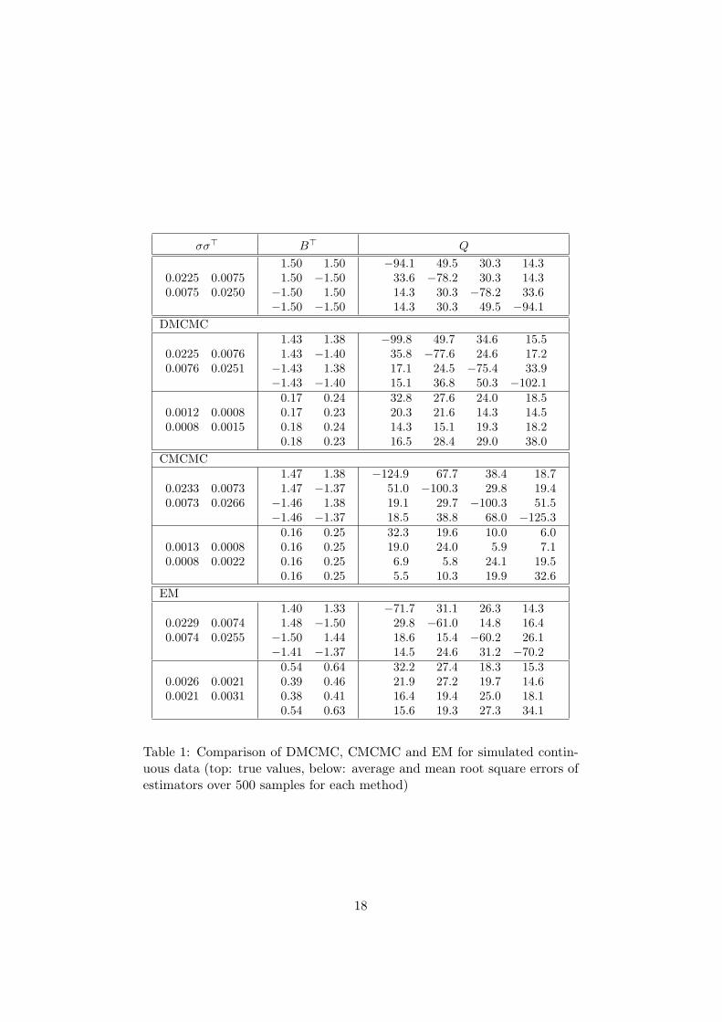
Table 1 provides a comparison of DMCMC, CMCMC, and the EM al-gorithm with respect to their statistical efficiency in parameter estimation.For all algorithms we evaluate the estimators of the drift, the covariancematrix and the rate matrix, by computing the average of all estimators overthe 500 replications as well as their root mean square errors. It turns outthat DMCMC yields appealing results for all parameters. The estimatesfor the drifts reflect the approximation error. Both CMCMC and the EMalgorithm fail to provide exact estimates for the rates, but they manage toidentify the underlying “structure”. However, they are clearly outperformedby DMCMC.

The results in Table 1 suggest that CMCMC tends to over-estimate therates. Indeed, further tests showed that especially for processes with highrates, the rate estimates sometimes do not enter into a stationary distribu-tion but continue growing which corresponds to inserting more and morejumps to the state process estimate. As this does not necessarily interferewith the average state estimation at each time (which works well never-theless), the likelihood function appears to carry insufficient information.Notice that to get aware of this phenomenon it is necessary to have theMCMC algorithm run for quite some time.

5.2.2 Daily Stock Index Data

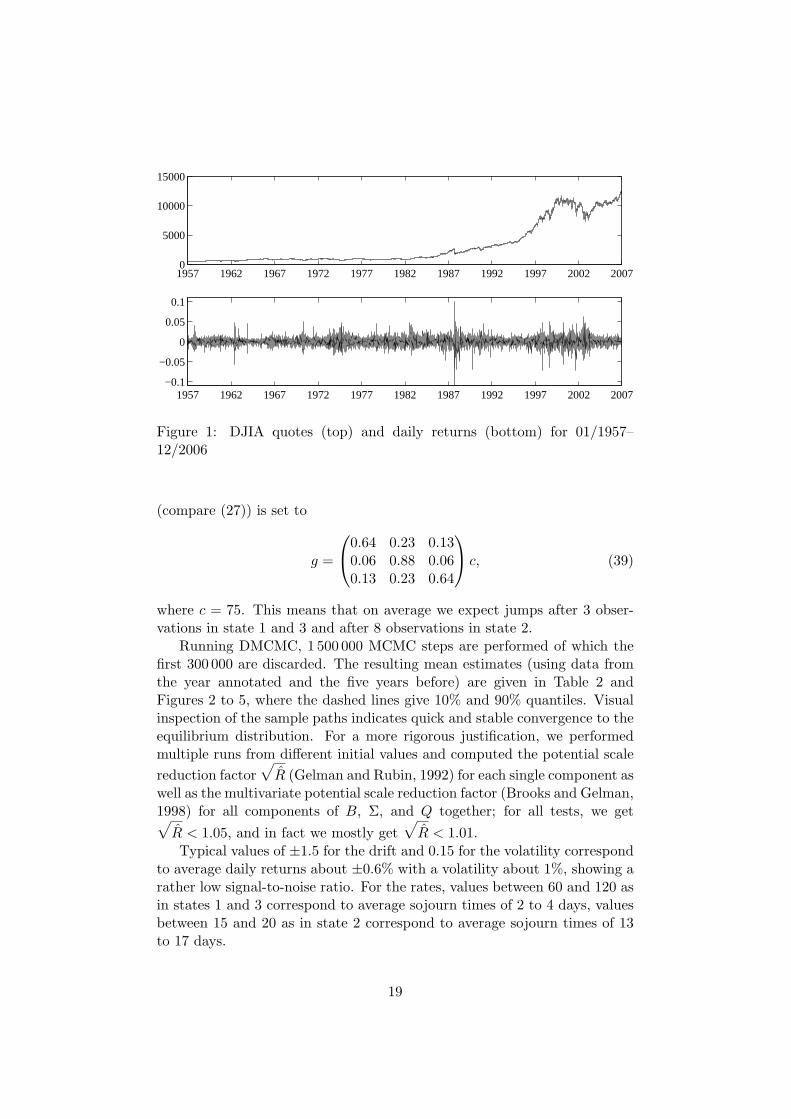
As an example for financial market data we consider daily data for the DowJones Industrial Average Index (DJIA) from 1957 to 2006 (see Figure 1).The data was organized in 45 overlapping blocks of six consecutive years’quotes, each comprising about 1500 data points.

For each set of six years’ quotes we employed DMCMC to fit a MSM.Assuming that there are d = 3 states seems to be a reasonable choice, asit allows for an up-, down-, and zero-state of the drift, while the number ofparameters is still moderate.

For each run, the parameters for the prior information of the drift areset to

m1 = q0.85 ∆t−1, m2 = m∆t−1, m3 = q0.15 ∆t−1, (37)

and sk = s = 0.25(m1−m3), where m, q0.15, and q0.85 denote mean and 15%as well as 85% quantiles of the daily returns under investigation, respectively.For the volatilities we set

Ξ(1) = Ξ(3) = 1.44 σ2∆t−1(ν − 1), Ξ(2) = 0.64 σ2∆t−1(ν − 1), (38)

and νk = ν = 3, where σ2 denotes the variance of the daily returns. For thetransition matrix, the matrix of parameters for the Dirichlet distribution

17

σσ> B> Q

0.0225 0.00750.0075 0.0250

1.50 1.501.50 −1.50

−1.50 1.50−1.50 −1.50

−94.1 49.5 30.3 14.333.6 −78.2 30.3 14.314.3 30.3 −78.2 33.614.3 30.3 49.5 −94.1

DMCMC

0.0225 0.00760.0076 0.0251

1.43 1.381.43 −1.40

−1.43 1.38−1.43 −1.40

−99.8 49.7 34.6 15.535.8 −77.6 24.6 17.217.1 24.5 −75.4 33.915.1 36.8 50.3 −102.1

0.0012 0.00080.0008 0.0015

0.17 0.240.17 0.230.18 0.240.18 0.23

32.8 27.6 24.0 18.520.3 21.6 14.3 14.514.3 15.1 19.3 18.216.5 28.4 29.0 38.0

CMCMC

0.0233 0.00730.0073 0.0266

1.47 1.381.47 −1.37

−1.46 1.38−1.46 −1.37

−124.9 67.7 38.4 18.751.0 −100.3 29.8 19.419.1 29.7 −100.3 51.518.5 38.8 68.0 −125.3

0.0013 0.00080.0008 0.0022

0.16 0.250.16 0.250.16 0.250.16 0.25

32.3 19.6 10.0 6.019.0 24.0 5.9 7.16.9 5.8 24.1 19.55.5 10.3 19.9 32.6

EM

0.0229 0.00740.0074 0.0255

1.40 1.331.48 −1.50

−1.50 1.44−1.41 −1.37

−71.7 31.1 26.3 14.329.8 −61.0 14.8 16.418.6 15.4 −60.2 26.114.5 24.6 31.2 −70.2

0.0026 0.00210.0021 0.0031

0.54 0.640.39 0.460.38 0.410.54 0.63

32.2 27.4 18.3 15.321.9 27.2 19.7 14.616.4 19.4 25.0 18.115.6 19.3 27.3 34.1

Table 1: Comparison of DMCMC, CMCMC and EM for simulated contin-uous data (top: true values, below: average and mean root square errors ofestimators over 500 samples for each method)

18

1957 1962 1967 1972 1977 1982 1987 1992 1997 2002 20070

5000

10000

15000

1957 1962 1967 1972 1977 1982 1987 1992 1997 2002 2007−0.1

−0.05

0

0.05

0.1

Figure 1: DJIA quotes (top) and daily returns (bottom) for 01/1957–12/2006

(compare (27)) is set to

g =

0.64 0.23 0.130.06 0.88 0.060.13 0.23 0.64

c, (39)

where c = 75. This means that on average we expect jumps after 3 obser-vations in state 1 and 3 and after 8 observations in state 2.

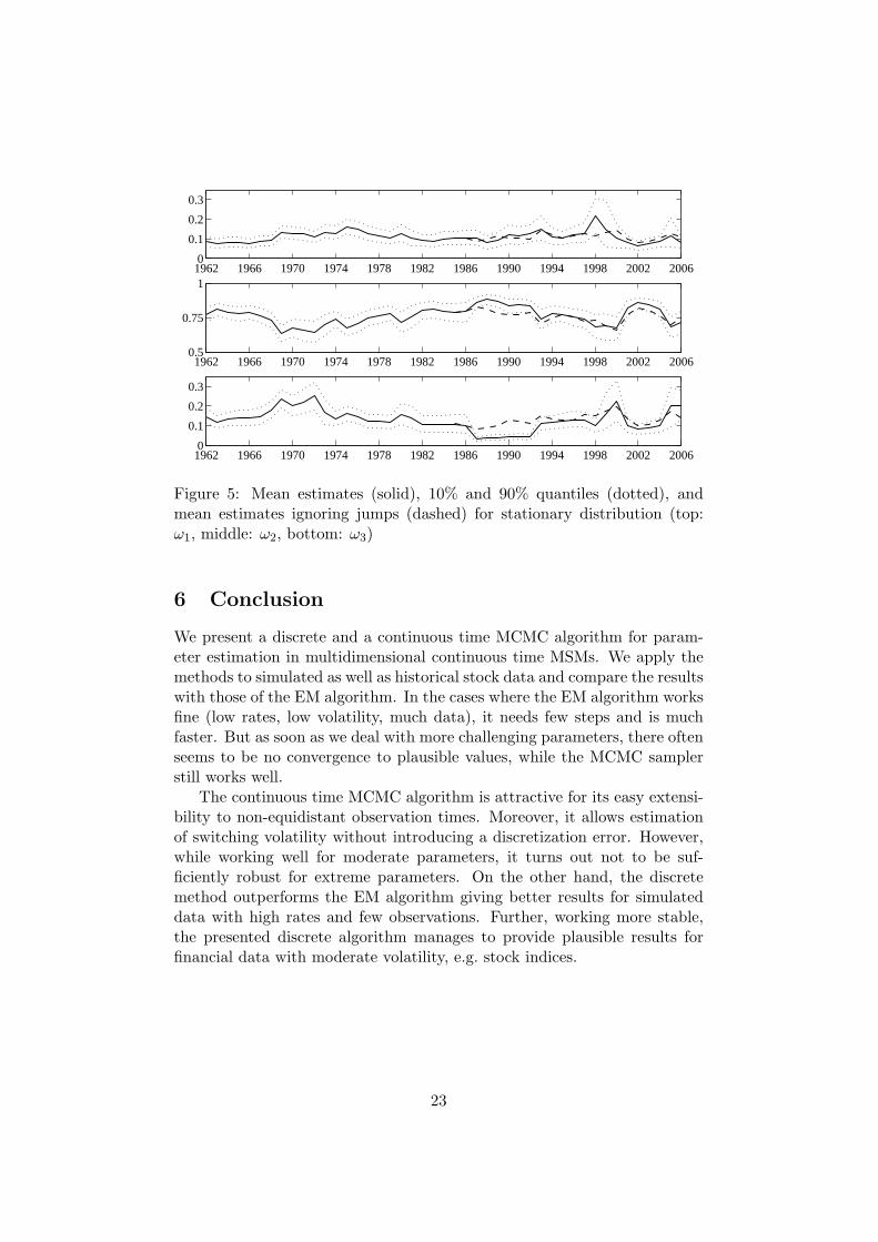
Running DMCMC, 1 500 000 MCMC steps are performed of which thefirst 300 000 are discarded. The resulting mean estimates (using data fromthe year annotated and the five years before) are given in Table 2 andFigures 2 to 5, where the dashed lines give 10% and 90% quantiles. Visualinspection of the sample paths indicates quick and stable convergence to theequilibrium distribution. For a more rigorous justification, we performedmultiple runs from different initial values and computed the potential scalereduction factor

√R (Gelman and Rubin, 1992) for each single component as

well as the multivariate potential scale reduction factor (Brooks and Gelman,1998) for all components of B, Σ, and Q together; for all tests, we get√R < 1.05, and in fact we mostly get

√R < 1.01.

Typical values of ±1.5 for the drift and 0.15 for the volatility correspondto average daily returns about ±0.6% with a volatility about 1%, showing arather low signal-to-noise ratio. For the rates, values between 60 and 120 asin states 1 and 3 correspond to average sojourn times of 2 to 4 days, valuesbetween 15 and 20 as in state 2 correspond to average sojourn times of 13to 17 days.

19

Time µ(1) µ(2) µ(3) σ(1) σ(2) σ(3) Q11 Q12 Q13 Q21 Q22 Q23 Q31 Q32 Q33

1962 1.09 0.29 -1.53 0.233 0.084 0.108 -116.0 62.1 53.9 1.5 -15.8 14.3 60.5 46.5 -107.01963 1.06 0.31 -1.61 0.249 0.082 0.088 -113.0 62.0 51.1 1.2 -14.3 13.1 62.5 58.2 -120.81964 1.04 0.27 -1.44 0.233 0.075 0.094 -112.5 62.4 50.2 1.5 -14.6 13.2 62.1 48.8 -110.91965 1.03 0.25 -1.27 0.228 0.070 0.098 -106.0 56.6 49.4 1.9 -13.6 11.7 53.5 42.6 -96.11966 1.14 0.22 -1.28 0.232 0.071 0.110 -101.3 54.1 47.2 1.6 -12.2 10.6 45.9 40.8 -86.71967 1.04 0.23 -1.28 0.224 0.069 0.101 -94.3 52.1 42.1 1.9 -14.0 12.1 46.6 42.3 -88.91968 1.13 0.25 -1.06 0.160 0.065 0.090 -111.8 67.0 44.8 3.6 -17.6 14.0 41.4 38.7 -80.11969 1.36 0.21 -1.20 0.110 0.062 0.091 -119.2 69.6 49.6 7.8 -27.2 19.4 47.2 34.0 -81.21970 1.46 0.19 -1.49 0.162 0.074 0.099 -108.1 66.5 41.7 6.3 -26.5 20.3 48.2 46.8 -95.01971 1.36 0.25 -1.45 0.180 0.080 0.094 -100.2 61.9 38.3 5.4 -31.4 26.0 41.3 56.7 -98.11972 1.17 0.39 -1.19 0.199 0.080 0.083 -92.9 60.1 32.8 5.0 -36.8 31.9 28.2 67.4 -95.61973 1.04 0.24 -1.83 0.217 0.087 0.087 -77.2 43.9 33.2 3.9 -25.9 21.9 47.6 70.8 -118.41974 2.05 0.05 -2.55 0.214 0.101 0.140 -107.5 38.0 69.5 5.3 -12.6 7.3 73.2 32.4 -105.71975 2.30 0.09 -2.54 0.199 0.105 0.142 -108.1 38.0 70.1 6.6 -16.2 9.6 80.8 30.3 -111.11976 2.20 0.13 -2.46 0.198 0.109 0.142 -107.4 39.4 68.1 5.8 -15.2 9.4 78.1 34.1 -112.21977 2.24 0.05 -2.62 0.199 0.114 0.145 -107.3 39.4 67.9 5.2 -12.1 6.9 78.9 33.3 -112.21978 2.38 0.04 -2.72 0.218 0.124 0.143 -115.7 51.0 64.7 5.9 -14.1 8.2 72.5 39.8 -112.31979 2.30 0.07 -2.48 0.216 0.117 0.145 -111.6 53.3 58.3 5.5 -13.6 8.1 63.9 44.0 -107.91980 1.83 0.17 -1.69 0.175 0.112 0.133 -119.1 68.9 50.3 8.3 -26.1 17.8 58.8 61.6 -120.41981 1.63 0.12 -1.62 0.176 0.113 0.134 -131.8 78.0 53.8 8.5 -23.9 15.3 50.0 68.8 -118.81982 1.78 0.05 -1.75 0.242 0.118 0.141 -110.2 55.2 55.0 5.7 -15.0 9.3 53.2 64.2 -117.51983 1.97 0.12 -1.72 0.244 0.125 0.145 -113.9 57.7 56.2 5.2 -14.2 9.0 55.5 61.1 -116.61984 2.06 0.03 -1.44 0.229 0.124 0.152 -122.9 65.1 57.8 8.1 -16.9 8.8 57.2 63.5 -120.71985 2.08 0.06 -1.35 0.227 0.122 0.150 -123.6 65.4 58.2 8.3 -16.9 8.5 58.6 59.9 -118.51986 1.89 0.06 -1.20 0.233 0.121 0.160 -120.1 64.9 55.2 8.6 -18.0 9.5 57.1 70.1 -127.21987 1.15 0.13 -2.05 0.271 0.129 0.763 -61.2 39.6 21.6 5.3 -7.2 1.8 53.1 63.4 -116.51988 1.43 0.16 -2.06 0.269 0.131 0.750 -92.1 58.6 33.5 6.1 -8.1 2.0 58.1 63.0 -121.11989 1.33 0.18 -2.01 0.265 0.126 0.750 -92.4 60.3 32.0 7.1 -9.5 2.4 58.1 65.0 -123.11990 0.73 0.26 -2.01 0.260 0.125 0.732 -74.2 49.3 25.0 8.1 -10.7 2.6 57.0 66.8 -123.81991 0.91 0.22 -2.11 0.269 0.131 0.729 -84.1 56.3 27.8 8.4 -11.4 3.0 58.0 69.8 -127.81992 0.80 0.16 -2.05 0.260 0.121 0.746 -73.5 49.8 23.7 8.2 -10.8 2.5 56.7 67.1 -123.81993 1.19 0.10 -1.35 0.173 0.099 0.271 -121.8 80.9 40.9 14.7 -27.6 12.9 66.2 75.7 -141.91994 1.38 0.13 -1.29 0.182 0.095 0.215 -129.9 83.6 46.3 9.4 -21.6 12.2 57.9 68.0 -125.91995 1.44 0.17 -1.35 0.180 0.088 0.174 -124.5 74.7 49.8 7.0 -19.4 12.4 59.4 59.0 -118.41996 1.31 0.18 -1.03 0.148 0.084 0.162 -122.8 74.7 48.1 8.9 -23.0 14.1 60.8 64.1 -124.91997 1.17 0.19 -1.04 0.145 0.086 0.207 -111.8 63.5 48.3 7.8 -20.2 12.4 64.9 54.4 -119.31998 0.62 0.25 -1.27 0.153 0.089 0.292 -68.9 35.8 33.1 11.1 -18.0 6.9 63.8 52.4 -116.21999 1.12 0.32 -1.03 0.243 0.102 0.231 -101.1 56.4 44.7 8.4 -21.1 12.7 51.0 50.2 -101.22000 1.42 0.38 -0.80 0.308 0.111 0.216 -113.9 59.7 54.2 5.4 -20.0 14.7 41.3 37.3 -78.62001 1.97 0.20 -1.94 0.234 0.145 0.335 -126.3 76.0 50.3 5.3 -13.5 8.2 59.6 51.1 -110.72002 2.48 0.14 -2.45 0.352 0.164 0.332 -117.0 63.0 54.1 3.0 -8.9 5.9 60.7 45.7 -106.42003 2.40 0.13 -2.39 0.335 0.160 0.309 -111.9 57.5 54.4 3.5 -9.7 6.1 61.7 45.7 -107.42004 2.13 0.08 -1.97 0.309 0.146 0.276 -110.4 54.5 55.9 4.0 -10.6 6.6 60.6 40.7 -101.42005 1.16 0.06 -0.62 0.334 0.114 0.229 -84.2 32.7 51.5 3.8 -10.2 6.4 33.3 19.9 -53.32006 1.24 0.10 -0.46 0.353 0.103 0.189 -82.5 33.2 49.3 2.6 -8.7 6.2 26.1 18.5 -44.6

Table 2: Estimation results for DJIA data: mean estimates for drift, volatil-ity, and rate matrix

20

1962 1966 1970 1974 1978 1982 1986 1990 1994 1998 2002 20060

2

4

1962 1966 1970 1974 1978 1982 1986 1990 1994 1998 2002 2006−0.2

0.2

0.6

1962 1966 1970 1974 1978 1982 1986 1990 1994 1998 2002 2006−4

−2

0

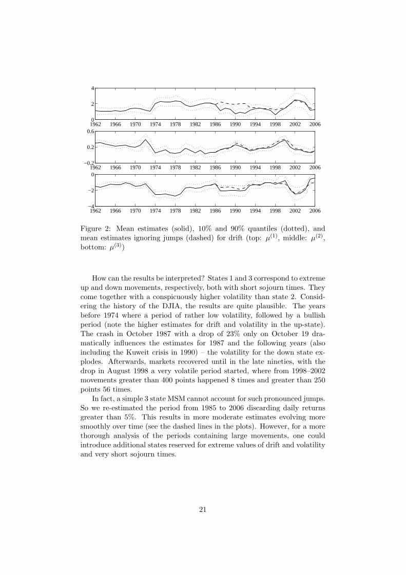
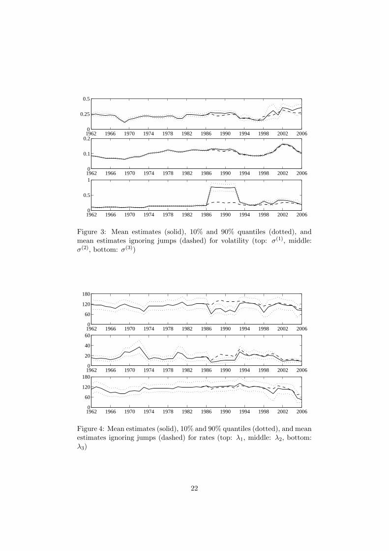
Figure 2: Mean estimates (solid), 10% and 90% quantiles (dotted), andmean estimates ignoring jumps (dashed) for drift (top: µ(1), middle: µ(2),bottom: µ(3))

How can the results be interpreted? States 1 and 3 correspond to extremeup and down movements, respectively, both with short sojourn times. Theycome together with a conspicuously higher volatility than state 2. Consid-ering the history of the DJIA, the results are quite plausible. The yearsbefore 1974 where a period of rather low volatility, followed by a bullishperiod (note the higher estimates for drift and volatility in the up-state).The crash in October 1987 with a drop of 23% only on October 19 dra-matically influences the estimates for 1987 and the following years (alsoincluding the Kuweit crisis in 1990) – the volatility for the down state ex-plodes. Afterwards, markets recovered until in the late nineties, with thedrop in August 1998 a very volatile period started, where from 1998–2002movements greater than 400 points happened 8 times and greater than 250points 56 times.

In fact, a simple 3 state MSM cannot account for such pronounced jumps.So we re-estimated the period from 1985 to 2006 discarding daily returnsgreater than 5%. This results in more moderate estimates evolving moresmoothly over time (see the dashed lines in the plots). However, for a morethorough analysis of the periods containing large movements, one couldintroduce additional states reserved for extreme values of drift and volatilityand very short sojourn times.

21

1962 1966 1970 1974 1978 1982 1986 1990 1994 1998 2002 20060

0.25

0.5

1962 1966 1970 1974 1978 1982 1986 1990 1994 1998 2002 20060

0.1

0.2

1962 1966 1970 1974 1978 1982 1986 1990 1994 1998 2002 20060

0.5

1

Figure 3: Mean estimates (solid), 10% and 90% quantiles (dotted), andmean estimates ignoring jumps (dashed) for volatility (top: σ(1), middle:σ(2), bottom: σ(3))

1962 1966 1970 1974 1978 1982 1986 1990 1994 1998 2002 20060

60

120

180

1962 1966 1970 1974 1978 1982 1986 1990 1994 1998 2002 20060

20

40

60

1962 1966 1970 1974 1978 1982 1986 1990 1994 1998 2002 20060

60

120

180

Figure 4: Mean estimates (solid), 10% and 90% quantiles (dotted), and meanestimates ignoring jumps (dashed) for rates (top: λ1, middle: λ2, bottom:λ3)

22

1962 1966 1970 1974 1978 1982 1986 1990 1994 1998 2002 20060

0.1

0.2

0.3

1962 1966 1970 1974 1978 1982 1986 1990 1994 1998 2002 20060.5

0.75

1

1962 1966 1970 1974 1978 1982 1986 1990 1994 1998 2002 20060

0.1

0.2

0.3

Figure 5: Mean estimates (solid), 10% and 90% quantiles (dotted), andmean estimates ignoring jumps (dashed) for stationary distribution (top:ω1, middle: ω2, bottom: ω3)

6 Conclusion

We present a discrete and a continuous time MCMC algorithm for param-eter estimation in multidimensional continuous time MSMs. We apply themethods to simulated as well as historical stock data and compare the resultswith those of the EM algorithm. In the cases where the EM algorithm worksfine (low rates, low volatility, much data), it needs few steps and is muchfaster. But as soon as we deal with more challenging parameters, there oftenseems to be no convergence to plausible values, while the MCMC samplerstill works well.

The continuous time MCMC algorithm is attractive for its easy extensi-bility to non-equidistant observation times. Moreover, it allows estimationof switching volatility without introducing a discretization error. However,while working well for moderate parameters, it turns out not to be suf-ficiently robust for extreme parameters. On the other hand, the discretemethod outperforms the EM algorithm giving better results for simulateddata with high rates and few observations. Further, working more stable,the presented discrete algorithm manages to provide plausible results forfinancial data with moderate volatility, e.g. stock indices.

23

Acknowledgment

The first author acknowledges financial support by the Austrian ScienceFund (FWF-projects S8305 and P17947-N12).

References

F. G. Ball, Y. Cai, J. B. Kadane, and A. O’Hagan. Bayesian inference forion-channel gating mechanisms directly from single-channel recordings,using Markov chain Monte Carlo. Proceedings of the Royal Society SeriesA, 455:2879–2932, 1999.

M. Bladt and M. Sørensen. Statistical inference for discretely observedMarkov jump processes. Journal of the Royal Statistical Society Series B,67(3):295–410, 2005.

R. J. Boys, D. A. Henderson, and D. J. Wilkinson. Detecting homogeneoussegments in DNA sequences by using hidden Markov models. AppliedStatistics, 49:269–285, 2000.

S. P. Brooks and A. Gelman. General methods for monitoring convergence ofiterative simulations. Journal of Computational and Graphical Statistics,7(4):434–455, 1998.

J. Buffington and R. J. Elliott. American options with regime switching. In-ternational Journal of Theoretical and Applied Finance, 5:497–514, 2002.

G. Celeux. Bayesian inference for mixtures: The label-switching problem.In R. Payne and P. J. Green, editors, COMPSTAT 98 – Proceedings inComputational Statistics, pages 227–232, Heidelberg, 1998. Physica.

G. Celeux, M. Hurn, and C. P. Robert. Computational and inferentialdifficulties with mixture posterior distributions. Journal of the AmericanStatistical Association, 95:957–970, 2000.

W. J. Culver. On the existence and uniqueness of the real logarithm of amatrix. Proceedings of the American Mathematical Society, 17:1146–1151,1966.

A. P. Dempster, N. M. Laird, and D. B. Rubin. Maximum likelihood fromincomplete data via the EM algorithm. Journal of the Royal StatisticalSociety Series B, 39(1):1–38, 1977.

G. Elfving. Zur Theorie der Markoffschen Ketten. Acta Social ScienceFennicae n. Series A, 2(8), 1937.

R. J. Elliott, L. Aggoun, and J. B. Moore. Hidden Markov Models – Esti-mation and Control, volume 29. Springer-Verlag, New York, 1995.

24

R. J. Elliott, W. C. Hunter, and B. M. Jamieson. Drift and volatility esti-mation in discrete time. Journal of Economic Dynamics and Control, 22:209–218, 1997.

R. J. Elliott, V. Krishnamurthy, and J. Sass. Moment based regressionalgorithm for drift and volatility estimation in continuous time Markovswitched models, 2006.

C. Engel and J. D. Hamilton. Long swings in the dollar: Are they in thedata and do markets know it? American Economic Review, 80(4):689–713, 1990.

S. Fruhwirth-Schnatter. Markov chain Monte Carlo estimation of classicaland dynamic switching and mixture models. Journal of the AmericanStatistical Association, 96(453):194–209, 2001a.

S. Fruhwirth-Schnatter. Fully Bayesian analysis of switching Gaussian statespace models. Annals of the Institute of Statistical Mathematics, 53(1):31–49, 2001b.

S. Fruhwirth-Schnatter. Finite Mixture and Markov Switching Models.Springer, New York, 2006.

A. Gelman and D. B. Rubin. Inference from iterative simulation using mul-tiple sequences. Statistical Science, 7:457–72, 1992.

X. Guo. An explicit solution to an optimal stopping problem with regimeswitching. Stochastic Processes and their Applications, 38:464–481, 2001.

M. Hurn, A. Justel, and C. P. Robert. Estimating mixtures of regressions.Journal of Computational and Graphical Statistics, 12:55–79, 2003.

R. B. Israel, J. S. Rosenthal, and J. Z. Wei. Finding generators for Markovchains via empirical transition matrices, with applications to credit rat-ings. Mathematical Finance, 11:245–265, 2001.

M. James, V. Krishnamurthy, and F. Le Gland. Time discretization ofcontinuous-time filters and smoothers for HMM parameter estimation.IEEE Transactions on Information Theory, 42:593–605, 1996.

A. Jasra, C. C. Holmes, and D. A. Stephens. Markov chain Monte Carlomethods and the label switching problem in Bayesian mixture modeling.Statistical Science, 20(1):50–67, 2005.

C.-J. Kim and C. R. Nelson. Has the U.S. economy become more stable?A Bayesian approach on a Markov-switching model of the business cycle.The Review of Econometrics and Statistics, 81:608–616, 1999.

25

J. F. C. Kingman. The imbedding problem for finite Markov chains.Zeitschrift fur Wahrscheinlichkeitstheorie und verwandte Gebiete, 1:14–24, 1962.

A. Kreinin and M. Sidelnikova. Regularization algorithms for transitionmatrices. Algo Research Quarterly, 4:23–40, 2001.

J. C. Liechty and G. O. Roberts. Markov chain Monte Carlo methods forswitching diffusion models. Biometrika, 88(2):299–315, 2001.

E. Otranto and G. M. Gallo. A nonparametric Bayesian approach to detectthe number of regimes in Markov switching models. Econometric Reviews,21(4):477–496, 2002.

R. Rosales, J. A. Stark, W. J. Fitzgerald, and S. B. Hladky. Bayesianrestoration of ion channel records using hidden Markov models. Biophys-ical Journal, 80(3):1088–1103, 2001.

J. Sass and U. G. Haussmann. Optimizing the terminal wealth under par-tial information: The drift process as a continuous time Markov chain.Finance and Stochastics, 8(4):553–577, 2004.

M. Stephens. Dealing with label switching in mixture models. Journal ofthe Royal Statistical Society Series B, 62(4):795–809, 2000.

26