markov chain monte carlo for rare-event simulation in heavy - kth

Markov chain Monte Carlo for rare-eventsimulation in heavy-tailed settings

Thorbjörn Gudmundsson

Abstract

In this thesis a method based on a Markov chain Monte Carlo (MCMC)algorithm is proposed to compute the probability of a rare event. The con-ditional distribution of the underlying process given that the rare event oc-curs has the probability of the rare event as its normalising constant. Us-ing the MCMC methodology a Markov chain is simulated, with that con-ditional distribution as its invariant distribution, and information aboutthe normalising constant is extracted from its trajectory.

The algorithm is described in full generality and applied to four differ-ent problems of computing rare-event probability. The first problem con-siders a random walk Y1+· · ·+Yn exceeding a high threshold, where the in-crements Y are independent and identically distributed and heavy-tailed.The second problem is an extension of the first one to a heavy-tailed ran-dom sum Y1 + · · · + YN exceeding a high threshold, where the numberof increments N is random and independent of Y1, . . . , Yn. The thirdproblem considers a stochastic recurrence equation Xn = AnXn−1 + Bnexceeding a high threshold, where the innovations B are independent andidentically distributed and heavy-tailed. The final problem considers theruin probability for an insurance company with risky investments.

An unbiased estimator of the reciprocal probability for each corre-sponding problem is constructed whose normalised variance vanishes asymp-totically. The algorithm is illustrated numerically and compared to exist-ing importance sampling algorithms.

iii

Sammanfattning

I denna avhandling presenteras en metod baserad på MCMC (Markovchain Monte Carlo) för att beräkna sannolikheten av en sällsynt hän-delse. Den betingade fördelningen för den underliggande processen givetatt den sällsynta händelsen inträffar har den sökta sannolikheten somsin normaliseringskonstant. Med hjälp av MCMC-metodiken skapas enMarkovkedja med betingade fördelningen som sin invarianta fördelningoch en skattning av normaliseringskonstanten baseras på den simuleradekedjan.

Algoritmen beskrivs i full generalitet och tillämpas på fyra exempel-problem. Första problemet handlar om en slumpvandring Y1 + · · · + Ynsom överskrider en hög tröskel, då stegen Y är oberoende, likafödelademed tungsvansad fördelning. Andra problemet är en utvidgning av detförsta till summa av ett stokastiskt antal termer. Tredje problemet be-handlar sannolikheten att lösningen Xn till en stokastisk rekurrensekva-tion Xn = AnXn−1 + Bn överskrider en hög tröskel då innovationernaB är oberoende, likafördelade med tungsvansad fördelning. Sista prob-lemet handlar om ruinsannolikhet för ett försäkringsbolag med riskfylldainvesteringar.

För varje exempelproblem konstrueras en väntevärdesriktig skattningav den reciproka sannolikheten. Skattningarna är effektiva i meningenatt deras normaliserade varians går mot noll. Vidare är de konstrueradeMarkovkedjorna likformigt ergodiska. Algoritmerna illustreras numerisktoch jämfös med existerande importance sampling algoritmer.

iv

AcknowledgementsI want to express my deepest appreciation for the support and help that I havereceived from my supervisor Henrik Hult. I am truly grateful for be given theopportunity to work under his guidance.

I want to offer my special thanks to colleagues at the faculty for their adviceand help, in particular Filip Lindskog and Tobias Rydén. Also want thank myfellow Ph.D. students, Björn, Johan and Pierre, for countless discussions andpractice sessions on the blackboard.

Finally, I want to thank my two special ones Rannveig and Gyða for theirimmense support and love.

v

Contents1 Introduction 1

1.1 Stochastic simulation . . . . . . . . . . . . . . . . . . . . . . . . . 21.1.1 Sampling a random variable . . . . . . . . . . . . . . . . . 21.1.2 Markov chain Monte Carlo . . . . . . . . . . . . . . . . . 41.1.3 Rare-event simulation . . . . . . . . . . . . . . . . . . . . 51.1.4 Importance sampling . . . . . . . . . . . . . . . . . . . . . 61.1.5 Heavy-tailed distributions . . . . . . . . . . . . . . . . . . 6

1.2 Markov chain Monte Carlo in rare-event simulation . . . . . . . . 71.2.1 Formulation . . . . . . . . . . . . . . . . . . . . . . . . . . 71.2.2 Controlling the normalised variance . . . . . . . . . . . . 81.2.3 Ergodic properties . . . . . . . . . . . . . . . . . . . . . . 101.2.4 Efficiency of the MCMC algorithm . . . . . . . . . . . . . 11

1.3 Outline and contribution of this thesis . . . . . . . . . . . . . . . 11

2 General Markov chain Monte Carlo formulation 132.1 Asymptotic efficiency criteria . . . . . . . . . . . . . . . . . . . . 14

3 Heavy-tailed Random Walk 153.1 A Gibbs sampler for computing P(Sn > an) . . . . . . . . . . . . 153.2 Constructing an efficient estimator . . . . . . . . . . . . . . . . . 183.3 Numerical experiments . . . . . . . . . . . . . . . . . . . . . . . . 19

4 Heavy-tailed Random Sum 214.1 A Gibbs sampler for computing P(SNn > an) . . . . . . . . . . . 224.2 Constructing an efficient estimator . . . . . . . . . . . . . . . . . 254.3 Numerical experiments . . . . . . . . . . . . . . . . . . . . . . . . 27

5 Stochastic Recurrence Equations 285.1 A Gibbs sampler for computing P(Xm > cn) . . . . . . . . . . . 285.2 Constructing an efficient estimator . . . . . . . . . . . . . . . . . 315.3 Numerical experiments . . . . . . . . . . . . . . . . . . . . . . . . 33

6 Ruin probability in an Insurance Model with Risky Invest-ments 356.1 A Gibbs sampler for computing the ruin probability . . . . . . . 366.2 Constructing an efficient estimator of the reciprocal ruin probability 36

vi

1 Introduction

Mathematical modelling of systems, in for instance natural sciences has been oneof the key building blocks of scientific understanding. The system of interest maybe the motion of the planets, the dynamic flow in a liquid, changes in stock pricesor the total amount of insurance claims made in a year. Often the model involvesthe system’s dynamic laws, long-time behavior and different possible scenarios.Such models nearly always include a parameter, or a set of parameters, which,though unknown in advance are still needed to calibrate the model to reality.Thus in order to have a fully specified model capable of forecasting the futureproperties or value, then one needs to measure the values of the the unknownparameters and thereby most likely introducing some measurement error. Thiserror is assumed to be random and thus the resulting forecast is the outcome ofa stochastic mathematical model.

With the ever increasing computational capacity in recent decades the mod-els are becoming more and more complex. Minor aspects that were ignored inthe simpler models can now be included in the computations, with increasingcomplexity. Researchers and practitioners alike strive to enhance current modelsand introduce more and more details to it, in the hope of increasing their fore-casting ability. Weather systems and finance processes are examples of modelsthat today are so involved that it is becoming difficult to give analytical andclosed form answers to property and forecasting questions. This has given riseto alternative approaches to handling such complex stochastic models, namelystochastic simulation.

Briefly, simulation is the process of sampling the underlying random fac-tors of a model to generate many instances of it, in order to make inferencesabout its properties. This has proved to be a powerful tool for computationin many academic fields such as physics, chemistry, economics, finance, in-surance. Generating instances of even the highly advanced stochastic models,multi-dimensional, non-linear and highly stochastic models can be done in afew milliseconds. Stochastic simulation has thus played its part in the scien-tific progress of recent decades and the simulation themselves has grown into anacademic field in its own right.

In physics, hypothesis are often tested and verified via a number of exper-iments. One experiment is carried out after another, and if sufficiently manyof the experiments support the hypothesis then it acquires a certain validityand becomes a theory. This was for instance the case at CERN in the summerof 2012, when the existence of the Higgs boson was confirmed through experi-ments which supported the old and well known hypothesis. However, one cannot always carry out experiments to validate hypotheses. Sometimes it is sim-ply impossible to replicate the model in reality, as is the case when studyingthe effects of global warming. Obviously, since we can only generate a singlephysical instance of the Earth, any simulations need to be done via computermodelling. To better reflect reality, the resolution needs to be high and manydifferent physical and meteorological factors need to be taken into account. Thesurface of the Earth is broken into 10km times 10km squares, each with itstemperature, air pressure, moisture and more. The dynamics of these weatherfactors need to be simulated with small times steps, perhaps many years intothe future. The Mathematics and Climate Research Network (MCRN) carriesout extensive stochastic simulations, replicating the Earth using different types

1

of scenarios to forecast possible climate changes. Clearly, this type of stochas-tic simulation is immensely computationally costly. This scientific work alonejustifies the importance of continuing research and improvement in the field ofstochastic simulation.

A subfield of stochastic simulation which deals with unlikely events of smallprobability is called rare-event simulation. Examples of rare-event simulationis when calculating capital requirements of a financing firm subject to BaselIII regulations, or of a insurance company subject to Solvency II regulations.Natural catastrophes such as avalanches, volcanic eruptions, to name but few,are also types rare-events for which we are interested in analysing. This is ofparticular importance when it comes to computationally heavy models. Thatis because, if an event is rare a computer needs many simulations to get a fairpicture of its frequency and the circumstances in which it occurred. And ifevery simulation takes up a lot of computational time, then a thorough studywould require a prohibitive amount of computer time would indeed be required.Therefore the improvement of efficient rare-event stochastic simulation is of highimportance.

The effect of heavy-tails in stochastic modelling is an important factor not tobe overlooked. By heavy tails we mean essentially that there is a non-negligibleprobability of extreme outcomes that differ significantly from the average. Suchextreme outcomes may have a considerable impact on a stochastic system. Forinstance, large claims due to a catastrophic event arrive at an insurance companycausing serious financial distress for the company. Similarly, large fluctuationson the financial market may lead to insolvency of financial institutions. In datanetworks the arrival of huge files may cause serious delays in the network, andso on.

This thesis presents a new methodology in rare-event simulation based onthe theory of Markov chain Monte Carlo. The general method presented inSection 2 makes very modest probabilistic assumptions and in subsequent sec-tions (random walk in Section 3, random sum in Section 4, stochastic recurrentequations in Section 5, ruin probability in Section6) is applied to few concreteexamples and shown to be efficient.

1.1 Stochastic simulation

In this section we introduce the basic tools in stochastic simulation, such aspseudo random number, the inversion method and Monte Carlo. We presentthe Markov chain Monte Carlo methodology and discuss briefly ergodicity.

1.1.1 Sampling a random variable

In this section we present the foundations of stochastic simulation, namely thegeneration of a pseudo random number by a computer and how it can be usedto sample a random variable via the inversion method.

Most statistical software programs provide methods for generating a uni-formly distributed pseudo random number on the interval, say, [0, 1]. Thesealgorithms are deterministic, at its core, and can only imitate the propertiesand behaviour of a uniformly distributed random variable. The early designsof such algorithms showed flaws in the sense that the pseudo random numbersgenerated followed a pattern which could easily be identified and predicted.

2

Nowadays there exists many highly advanced algorithms that generate pseudorandom numbers, mimicking a true random number quite well. For the purposesof this thesis we assume the existence of an algorithm producing a uniformlydistributed pseudo random number, and ignore any deficiencies and errors aris-ing from the algorithm. In short, we assume that we can sample a perfectlyuniformly distributed random variable in some computer program. For a morethorough and detailed discussion we refer to [48].

Now consider a random variable X and denote by F its probability distri-bution. Say we would like, via some computer software, to sample the randomvariable X.One approach is the inversion method. The inversion method in-volves only applying the quantile function to uniformly random variable. Moreformally the algorithm is as follows.

1. Sample U from the standard uniform distribution.

2. Compute Z = F−1(U),

where F−1 = min{x | F (x) ≥ p}. The random variable Z has the same distri-bution as X as the following display shows.

P(Z ≤ x) = P(F−1{U} ≤ x) = P(U ≤ F (x)) = F (x).

The method can easily be extended to sampling X conditioned on being largerthan some constant c. Meaning that we want to sample from the conditionaldistribution

P(X ∈ · | X > c).

The algorithm is formally as follows.

1. Sample U from the standard uniform distribution.

2. Compute Z = F−1((

1− F (c))U + F (c)

).

The distribution of Z is given by,

P(Z ≤ x) = P((1− F (c))U + F (c) ≤ F (x)

)= P

(U ≤ F (x)− F (c)

1− F (c)

)=

F (x)− F (c)1− F (c)

=P(c ≤ X ≤ x)P(X > c)

= P(X ≤ x | X > c).

Thus the inversion method provides a simple way of sampling a random variable,conditioned on being larger than c, based solely on the generation of a uniformlydistributed random number.

The most standard tool for stochastic simulation is the Monte Carlo tech-nique. The power of Monte Carlo is its simplicity. Let X be a random variableand assume we want to compute the probability that {X ∈ A} for some Borelset A. The idea of Monte Carlo is to sample independent and identically dis-tributed copies of random variable, say X1, . . . , Xn and simply compute thefrequency of hitting the set A. More formally, the Monte Carlo estimator ofP(X ∈ A) is given by

p̂ =1

n

n∑i=1

I{Xi ∈ A}.

While the procedure is easy and simple there are drawbacks that will be dis-cussed in Section 1.1.3.

3

1.1.2 Markov chain Monte Carlo

In this section we present a simulation technique called Markov chain MonteCarlo (MCMC) for sampling a random variable X despite only having limitedinformation about its distribution.

MCMC is typically useful when sampling a random variable X having adensity f that is only known up to a constant, say

f(x) =π(x)

c,

where π is known but c =∫π(x)dx is unknown. This may seem strange setup

at first but once noted that the normalising constant c may be difficult to deter-mine, say there is no known closed form for c, then this is a natural formulation.An example of this type of setup can be found in Bayesian statistics and hiddenMarkov chains.

In short, the basic idea of sampling via MCMC is to generate a Markov chain(Yt)t≥0 whose invariant density is the same as of X, namely f . There existsplentiful of MCMC algorithms but we shall only name two in this thesis, theMetropolis-Hastings algorithm and the Gibbs algorithm.

The method first laid out by Metropolis [41] and then extended by Hastings[26] is based on a proposal density, which we shall denote by g. Firstly theMarkov chain (Yt)t≥0 is initialised with some Y0 = y0. The idea behind theMetropolis-Hastings algorithm is to generate a proposal state Z using the pro-posal density g. The next state of the Markov chain is then assigned the valueZ with the acceptance probability α, otherwise the next state of the Markovchain stays unchanged (i.e. retains the same value as before). More formallythe algorithm is as follows.

Algorithm 1.1. Set Y0 = y0. For a given state Yk, for some k = 0, 1, . . ., thenext state Yk+1 is sampled as follows

1. Sample Z from the proposal density g.

2. Let

Yk+1 =

{Z with probability α(Yk, Z)Yk otherwise

where α(y, z) = min{1, r(y, z)}, r(y, z) = π(z)g(z,y)π(y)g(y,z) .

This algorithm produces a Markov chain (Yk)k≥1 whose invariant density isgiven by f . Fore more details on the Metropolis-Hastings algorithm we refer to[3] and [23].

Another method of MCMC sampling is the Gibbs sampler, which was orig-inally introduced by Geman and Geman in [22]. If the random variable X ismulti-dimensional X = (X1, . . . , Xd), the Gibbs sampler updates each com-ponent at the time by sampling from the conditional marginal distributions.Let fk|6k(xk | x1, . . . , xk−1, xk+1, . . . , xd), k = 1, . . . , d, denote the conditionaldensity of Xk given X1, . . . , Xk−1, Xk+1, . . . , Xd. The Gibbs sampler can beviewed as a special case of the Metropolis-Hastings algorithm where, givenYk = (Yk,1, . . . , Yk,d), one first updates Yk,1 from the conditional density f1|61(· |Yk,2, . . . , Yk,d), then Yk,2 from the conditional density f2|62(· | Yk+1,1, Yk,3, . . . , Yk,d),

4

etc. By sampling from these proposal densities the acceptance probability is al-ways equal to 1, so no acceptance step is needed.

An important property of a Markov chain is its ergodicity. Informally, er-godicity measures the how quickly the Markov chain mixes and thus how soonthe dependency of the chain dies out. This is a highly desired property sincegood mixing speeds up the convergence of the Markov chain.

1.1.3 Rare-event simulation

In some specific cases we are interested in computing the probability of a rareevent. This may be the probability of ruin of a financial company due to random-ness in the future value of assets and liabilities. The multidimensional system ofinvestments and bonds may be so complex that a simulation of the catastrophicevent of a ruin may be feasible. For another example, consider a graph of somesort and say we send out a particle on a random walk along the graph givensome starting position. Computing the small, and quickly decreasing probabil-ity, of that particle returning to its starting position may be of interest as it isan indicator of that graph’s dimension. For these reasons and many other, thecomputation of the probability for a rare-event is relevant.

Consider an unbiased estimator p̂ of the probability p and investigate its per-formance as the probability gets smaller p→ 0. A useful performance measureis the relative error:

RE(p̂) =Std(p̂)p

.

An estimator is said to have vanishing relative error if RE(p̂) → 0 as p → 0and bounded relative error if RE(p̂) <∞ as p→ 0.

It is well known that the Monte Carlo estimator is inefficient for computingrare-event probabilities as the following argument shows. Let X be a givenrandom variable with distribution function F and say we would like to computep = P(X ∈ A). We sample number of i.i.d. copies of X, denoted by X1, . . . , Xn

and compute

p̂ =1

n

n∑i=1

I{Xi ∈ A}.

The variance of the estimator is Var(p̂) = 1np(1−p), which clearly tends to zero

as n → ∞ but that is not main concern here. What is more interesting is itsrelative error as the probability p tends to zero. Its relative error is given by

Std(p̂)p

=

√1

n

(1p− 1).

The relative error tends to infinity as p → 0. Thus making the Monte Carloalgorithm very costly when it comes to rare-event simulation. For example, if arelative error at 1% is desired and the probability is of order 10−6 then we needto take n such that

√(106 − 1)/n ≤ 0.01. This implies that n ≈ 1010 which is

infeasible on most computer systems.To improve on standard Monte Carlo a control mechanism needs to be in-

troduced that steer the samples towards the relevant part of the state space,thereby increasing the relevance of each sample. There are several ways to dothis, for instance by importance sampling described briefly below, or by splitting

5

schemes as by L’Ecyer [39], or interacting particle systems as by Del Moral in[14].

1.1.4 Importance sampling

The simulation method of importance sampling comes as a remedy to the prob-lem arising in rare-event simulation. The underlying problem of the Monte Carlosimulation for rare-event studies is the fact that we get too few samples in theimportant part of the output space, meaning that we get too few samples where{X ∈ A}. The basic idea of importance sampling is that instead of samplingfrom the original distribution F the X1, . . . , Xn are sampled from a so-calledsampling distribution, say G. The sampling distribution G is chosen such thatwe obtain more samples where {X ∈ A}. The importance sampling is then sim-ply the average of hitting the event, weighted with the relevant Radon-Nikodymderivative,

p̂IS =1

n

n∑i=1

dF

dGI{Xi ∈ A}.

This is a unbiased and consistent estimator since

EG[p̂IS] =

∫A

dF

dGdG = P(X ∈ A).

The main difficulty in importance sampling is to design the sampling distri-bution. Traditionally the functionality and reliability of new stochastic simu-lation algorithms is “proved” by running extensive numerical experiments. Butnumerical evidence alone is insufficient. There are numerous examples wherethe standard heuristics fail and the numerical evidence indicates that the al-gorithm has converged when, in fact, it is severely biased [24]. The limitedevidence provided by simply running numerical experiments has generated theneed for a deeper theoretical understanding and analysis of the performanceof stochastic simulation algorithms. Over the last decade mathematical toolsfrom stability theory and control theory have been developed with the aim totheoretically quantify the performance of stochastic simulation algorithms forcomputing probabilities of rare events. In the context of importance samplingtwo main approaches have been studied; the subsolution approach, based oncontrol theory, by Dupuis, Wang, and collaborators, see e.g. [18, 19, 17], andthe approach based on Lyapunov functions and stability theory by Blanchet,Glynn, and others, see [5, 6, 7, 10].

In the theoretical work on efficient importance sampling an algorithm is saidto be efficient if relative error per sample, Std(p̂)/p does not grow too rapidlyas p ↓ 0.

1.1.5 Heavy-tailed distributions

In this thesis we consider in particular probability distributions F with heavy-tails. The notion of heavy tails refers to the rate of decay of the tail F = 1−Fof a distribution function F . A popular class of heavy-tailed distributions is theclass of subexponential distributions. A distribution function F supported onthe positive axis is said to belong to the subexponential distributions if

limx→∞

P(X1 +X2 > x)

P(X1 > x)= 2,

6

for independent random variables X1 and X2 with distribution F . A subclassof the subexponential distributions is the regularly varying distributions. F iscalled regularly varying (at ∞) with index −α ≤ 0 if

limt→∞

F (tx)

F (t)= x−α, for all x > 0.

The heavy-tailed distributions are often described with the “one big jump”analogy, meaning that the event of a sum of heavy-tailed random variables beinglarge is dominated by the case of one of the variables being very large whilstthe rest are relatively small. This is in sharp contrast to the case of light-tails,where the same event is dominated by the case of every variable contributingequally to the total. As a reference to the one big jump analogy we refer thereader to [28, 30, 15].

This one big jump phenomena has been observed in empirical data. Forinstance, when we consider stock market indices such as Nasdaq, Dow Jonesetc. it turns out that the distribution of daily log returns typically has a heavyleft tail, see Hult et al. in [29]. Another example is the well studied Danish fireinsurance data, which consists of real-life claims caused by industrial fires inDenmark. While the arrivals of claims is showed to be not far from Poisson, theclaim size distribution shows clear heavy-tail behavior. The data set is analysedby Mikosch in [43] and the tail of the claim size is shown to be fit well with aPareto distribution.

Stochastic simulation in the presence of heavy-tailed distributions has beenstudied with much interest in recent years. The conditional Monte Carlo tech-nique was applied on this setting by Asmussen et al. [2, 4]. Dupuis et al. [16] usedimportance sampling algorithm in a heavy-tailed setting. Finally we mentionthe work of Blanchet et al. considering heavy-tailed distributions in [11, 8].

1.2 Markov chain Monte Carlo in rare-event simulationIn this section we describe a new methodology based on Markov chain MonteCarlo (MCMC), for computing probabilities of rare events. A more generalversion of the algorithm, for computing expectations, is provided in Section 2along with a precise asymptotic efficiency criteria.

1.2.1 Formulation

Let X be a real-valued random variable with distribution F and density f withrespect to the Lebesgue measure. The problem is to compute the probability

p = P(X ∈ A) =∫A

dF . (1.1)

The event {X ∈ A} is thought of as rare in the sense that p is small. Let FA bethe conditional distribution of X given X ∈ A. The density of FA is given by

dFAdx

(x) =f(x)I{x ∈ A}

p. (1.2)

Consider a Markov chain (Xt)t≥0 with invariant density given by (1.2). Such aMarkov chain can be constructed by implementing an MCMC algorithm suchas a Gibbs sampler or a Metropolis-Hastings algorithm, see e.g. [3, 23].

7

To construct an estimator for the normalising constant p, consider a non-negative function v, which is normalised in the sense that

∫Av(x)dx = 1. The

function v will be chosen later as part of the design of the estimator. For anychoice of v the sample mean,

1

T

T−1∑t=0

v(Xt)I{Xt ∈ A}f(Xt)

,

can be viewed as an estimate of

EFA

[v(X)I{X ∈ A}

f(X)

]=

∫A

v(x)

f(x)

f(x)

pdx =

1

p

∫A

v(x)dx =1

p.

Thus,

q̂T =1

T

T−1∑t=0

u(Xt), where u(Xt) =v(Xt)I{Xt ∈ A}

f(Xt), (1.3)

is an unbiased estimator of q = p−1. Then p̂T = q̂−1T is an estimator of p.The expected value above is computed under the invariant distribution FA

of the Markov chain. It is implicitly assumed that the sample size T is suffi-ciently large that the burn-in period, the time until the Markov chain reachesstationarity, is negligible or alternatively that the burn-in period is discarded.Another remark is that it is theoretically possible that all the terms in the sumin (1.3) are zero, leading to the estimate q̂T = 0 and then p̂T = ∞. To avoidsuch nonsense one can simply take p̂T as the minimum of q̂−1T and one.

There are two essential design choices that determine the performance of thealgorithm: the choice of the function v and the design of the MCMC sampler.The function v influences the variance of u(Xt) in (1.3) and is therefore of mainconcern for controlling the rare-event properties of the algorithm. It is desirableto take v such that the normalised variance of the estimator, given by p2 Var(q̂T ),is not too large. The design of the MCMC sampler, on the other hand, is crucialto control the dependence of the Markov chain and thereby the convergence rateof the algorithm as a function of the sample size. To speed up simulation it isdesirable that the Markov chain mixes fast so that the dependence dies outquickly.

1.2.2 Controlling the normalised variance

This section contains a discussion on how to control the performance of theestimator q̂T by controlling its normalised variance.

For the estimator q̂T to be useful it is of course important that its varianceis not too large. When the probability p to be estimated is small it is reasonableto ask that Var(q̂T ) is of size comparable to q2 = p−2, or equivalently, that thestandard deviation of the estimator is roughly of the same size as p−1. To thisend the normalised variance p2 Var(q̂T ) is studied.

Let us consider Var(q̂T ). With

u(x) =v(x)I{x ∈ A}

f(x),

8

it follows that

p2 VarFA(q̂T ) = p2 VarFA

( 1

T

T−1∑t=0

u(Xt))

= p2( 1

TVarFA

(u(X0)) +2

T 2

T−1∑t=0

T−1∑s=t+1

CovFA(u(Xs), u(Xt))

), (1.4)

Let us for the moment focus our attention on the first term. It can be writtenas

p2

TVarFA

(u(X0)

)=

p2

T

(EFA

[u(X0)

2]−EFA

[u(X0)

]2)=

p2

T

(∫ ( v(x)f(x)

I{x ∈ A})2FA(dx)−

1

p2

)=

p2

T

(∫ v2(x)

f2(x)I{x ∈ A}f(x)

pdx− 1

p2

)=

1

T

(∫A

v2(x)p

f(x)dx− 1

).

Therefore, in order to control the normalised variance the function v must bechosen so that

∫Av2(x)f(x) dx is close to p−1. An important observation is that the

conditional density (1.2) plays a key role in finding a good choice of v. Lettingv be the conditional density in (1.2) leads to∫

A

v2(x)

f(x)dx =

∫A

f2(x)I{x ∈ A}p2f(x)

dx =1

p2

∫A

f(x)dx =1

p,

which implies,p2

TVarFA

(u(X)

)= 0.

This motivates taking v as an approximation of the conditional density (1.2).This is similar to the ideology behind choosing an efficient importance samplingestimator.

If for some set B ⊂ A the probability P(X ∈ B) can be computed explicitly,then a candidate for v is

v(x) =f(x)I{x ∈ B}P(X ∈ B)

,

the conditional density of X given X ∈ B. This candidate is likely to performwell if P(X ∈ B) is a good approximation of p. Indeed, in this case∫

A

v2(x)

f(x)dx =

∫A

f2(x)I{x ∈ B}P(X ∈ B)2f(x)

dx =1

P(X ∈ B)2

∫B

f(x)dx =1

P(X ∈ B),

which will be close to p−1.Now, let us shift emphasis to the covariance term in (1.4). As the samples

(Xt)T−1t=0 form a Markov chain the Xt’s are dependent. Therefore the covariance

term in (1.4) is non-zero and may not be ignored. The crude upper bound

CovFA(u(Xs), u(Xt)) ≤ VarFA

(u(X0)),

9

leads to the upper bound

2p2

T 2

T−1∑t=0

T−1∑s=t+1

CovFA(u(Xs), u(Xt)) ≤ p2

(1− 1

T

)VarFA

(u(X0))

for the covariance term. This is a very crude upper bound as it does not decayto zero as T → ∞. But, at the moment, the emphasis is on small p so wewill proceed with this upper bound anyway. As indicated above the choice of vcontrols the term p2 VarFA

(u(X0)). We conclude that the normalised variance(1.4) of the estimator q̂T is controlled by the choice of v when p is small.

1.2.3 Ergodic properties

As we have just seen the choice of the function v controls the normalised varianceof the estimator for small p. The design of the MCMC sampler, on the otherhand, determines the strength of the dependence in the Markov chain. Strongdependence implies slow convergence which results in a high computational cost.The convergence rate of MCMC samplers can be analysed within the theoryof ϕ-irreducible Markov chains. Fundamental results for ϕ-irreducible Markovchains are given in [42, 44]. We will focus on conditions that imply a geometricconvergence rate. The conditions given below are well studied in the context ofMCMC samplers. Conditions for geometric ergodicity in the context of Gibbssamplers have been studied by e.g. [12, 51, 52], and for Metropolis-Hastingsalgorithms by [40].

A Markov chain (Xt)t≥0 with transition kernel p(x, ·) = P(Xt+1 ∈ · | Xt =x) is ϕ-irreducible if there exists a measure ϕ such that

∑t p

(t)(x, ·) � ϕ(·),where p(t)(x, ·) = P(Xt ∈ · | X0 = x) denotes the t-step transition kernel and� denotes absolute continuity. A Markov chain with invariant distribution π iscalled geometrically ergodic if there exists a positive function M and a constantr ∈ (0, 1) such that

‖p(t)(x, ·)− π(·)‖TV ≤M(x)rt, (1.5)

where ‖ · ‖TV denotes the total-variation norm. This condition ensures that thedistribution of the Markov chain converges at a geometric rate to the invariantdistribution. If the function M is bounded, then the Markov chain is said to beuniformly ergodic. Conditions such as (1.5) may be difficult to establish directlyand are therefore substituted by suitable minorisation or drift conditions. Aminorisation condition holds on a set C if there exist a probability measure ν,a positive integer t0, and δ > 0 such that

p(t0)(x,B) ≥ δν(B),

for all x ∈ C and Borel sets B. In this case C is said to be a small set.Minorisation conditions have been used for obtaining rigorous bounds on theconvergence of MCMC samplers, see e.g. [49].

If the entire state space is small, then the Markov chain is uniformly er-godic. Uniform ergodicity does typically not hold for Metropolis samplers, seeMengersen and Tweedie in [40] Theorem 3.1. Therefore useful sufficient con-ditions for geometric ergodicity are often given in the form of drift conditions[12, 40]. Drift conditions, established through the construction of appropriateLyapunov functions, are also useful for establishing central limit theorems forMCMC algorithms, see [34, 42] and the references therein.

10

1.2.4 Efficiency of the MCMC algorithm

Roughly speaking, the arguments given above lead to the following desired prop-erties of the estimator.

1. Rare event efficiency: Construct an unbiased estimator q̂T of p−1 accord-ing to (1.3) by finding a function v which approximates the conditionaldensity (1.2). The choice of v controls the normalised variance of theestimator.

2. Large sample efficiency: Design the MCMC sampler, by finding an ap-propriate Gibbs sampler or a proposal density in the Metropolis-Hastingsalgorithm, such that the resulting Markov chain is geometrically ergodic.

1.3 Outline and contribution of this thesis

The outline and contribution of the thesis are as follows.

a. General formulation of the algorithm in Section 2. In this section wepresent the formal methodology in how to set up the MCMC simulationfor efficient rare-event computation. The probabilistic assumptions madeare mild and the setting is for instance not restricted to heavy-tails. Thetwo essential design choices are highlighted. Corresponding to rare-eventefficiency and large sample efficiency.

b. Application to heavy-tailed random walks in Section 3. In this section theMCMC methodology is applied to the problem of computing

pn = P(Y1 + · · ·+ Yn > an),

where an →∞ sufficiently fast so that the probability tends to zero. Theincrements Y are assumed to be heavy-tailed. We present a Gibbs samplerto produce a Markov chain whose invariant distribution is the conditionaldistribution

P((Y1, . . . , Yn) ∈ · | Y1 + · · ·+ Yn > an

).

The Markov chain is shown to preserve stationarity and uniformly ergodic,ensuring the large sample efficiency. In addition we design an estimatorfor 1/pn having vanishing normalised variance. Numerical experimentsperformed and comparison made between MCMC and best-performingexisting importance sampling estimators as well as standard Monte Carlo.

c. Application to heavy-tailed random sums in Section 4. In this section theMCMC methodology is applied to the problem of computing

pn = P(Y1 + · · ·+ YNn> aNn

),

where N is a random variable and aN → ∞ sufficiently fast so that theprobability tends to zero. The increments Y are assumed to be heavy-tailed. We present a Gibbs sampler to produce a Markov chain whoseinvariant distribution is the conditional distribution

P((N,Y1, . . . , YN ) ∈ · | Y1 + · · ·+ YN > aN

).

11


d. Application to stochastic recurrent equations in Section 5. In this sectionthe MCMC methodology is applied to the problem of computing pn =P(Xn > an), where

Xn = AnXn−1 +Bn,X0 = 0,

and an →∞ sufficiently fast so that the probability tends to zero. The in-crements B are assumed to be regularly varying of index α and E[Aα+ε] <∞ for some ε > 0. We present a Gibbs sampler to produce a Markov chainwhose invariant distribution is the conditional distribution

P((A2, . . . , An, B1, . . . , Bn) ∈ · | Xn > an

).


e. Application to an insurance model with risky investments in Section 6. Inthis section the MCMC methodology is applied to the problem of com-puting the probability of ruin P(sup1≤k≤nWk > un), where W is thediscounted loss process.

A paper titled Markov chain Monte Carlo for computing rare-event proba-bilities for a heavy-tailed random walk by Gudmundsson and Hult [25] basedon Sections 2, 3, and 4 in the thesis has been accepted for publication in theJournal of Applied Probability in June 2014.

12

2 General Markov chain Monte Carlo formula-tion

In this section the Markov chain Monte Carlo ideas are applied to the problemof computing an expectation. Here the setting is general, for instance, there isno assumption that densities with respect to Lebesgue measure exist.

Let X be a random variable with distribution F and h be a non-negativeF -integrable function. The problem is to compute the expectation

θ = E[h(X)

]=

∫h(x)dF (x).

In the special case when F has density f and h(x) = I{x ∈ A} this problemreduces to the simpler problem of computing the probability in (1.1). illustratedin Section 1.2.

The analogue of the conditional distribution in (1.2) is the distribution Fhgiven by

Fh(B) =1

θ

∫B

h(x)dF (x), for measurable sets B.

Consider a Markov chain (Xt)t≥0 having Fh as its invariant distribution. Todefine an estimator of θ−1, consider a probability distribution V with V � Fh.Then it follows that V � F and it is assumed that the density dV/dF is known.Consider the estimator of ζ = θ−1 given by

ζ̂T =1

T

T−1∑t=0

u(Xt), where u(x) =1

θ

dV

dFh(x). (2.1)

Note that u does not depend on θ because V � Fh and therefore

u(x) =1

θ

dV

dFh(x) =

1

h(x)

dV

dF(x),

for x such that h(x) > 0. The estimator (2.1) is a generalisation of the estimator(1.3) where one can think of v as the density of V with respect to Lebesguemeasure. An estimator of θ can then constructed as θ̂T = ζ̂−1T .

The variance analysis of ζ̂T follows precisely the steps outlined in Section1.2. The normalised variance is

θ2 VarFh(ζ̂T ) =

θ2

TVarFh

(u(X0)

)+

2θ2

T 2

T−1∑t=0

T−1∑s=t+1

CovFh

(u(Xs), u(Xt)

), (2.2)

where the first term can be rewritten, similarly to the display (1.4), as

θ2

TVarFh

(u(X0)

)=

1

T

(EV

[ dVdFh

]− 1).

The analysis above indicates that an appropriate choice of V is such thatEV [

dVdFh

] is close to 1. Again, the ideal choice would be taking V = Fh leading tozero variance. This choice is not feasible but nevertheless suggests selecting V asan approximation of Fh. As already noted this is similar to the ideology behindchoosing an efficient importance sampling estimator. The difference being thathere V � F is required whereas in importance sampling F needs be absolutelycontinuous with respect to the sampling distribution. The crude upper boundfor the covariance term in (2.2) is valid, just as in Section 1.2.

13

2.1 Asymptotic efficiency criteriaAsymptotic efficiency can be conveniently formulated in terms of a limit criteriaas a large deviation parameter tends to infinity. As is customary in problemsrelated to rare-event simulation the problem at hand is embedded in a sequenceof problems, indexed by n = 1, 2, . . . . The general setup is formalised as follows.

Let (X(n))n≥1 be a sequence of random variables with X(n) having distri-bution F (n). Let h be a non-negative function, integrable with respect to F (n),for each n. Suppose

θ(n) = E[h(X(n))

]=

∫h(x)dF (n)(x)→ 0,

as n→∞. The problem is to compute θ(n) for some large n.Denote by F

(n)h the distribution with dF

(n)h /dF (n) = h/θ(n). For the nth

problem, a Markov chain (X(n)t )T−1t=0 with invariant distribution F (n)

h is gener-ated by an MCMC algorithm. The estimator of ζ(n) = (θ(n))−1 is based on aprobability distribution V (n), such that V (n) � F

(n)h , with known density with

respect to F (n). An estimator ζ̂(n)T of ζ is given by

ζ̂(n)T =

1

T

T−1∑t=0

u(n)(X(n)t ),

where

u(n)(x) =1

h(x)

dV (n)

dF (n)(x).

The heuristic efficiency criteria in Sections 1.2 can now be rigorously formu-lated as follows:

1. Rare-event efficiency: Select the probability distributions V (n) such that

(θ(n))2 VarF

(n)h

(u(n)(X))→ 0, as n→∞.

2. Large sample size efficiency: Design the MCMC sampler, by finding an ap-propriate Gibbs sampler or a proposal density for the Metropolis-Hastingsalgorithm, such that, for each n ≥ 1, the Markov chain (X

(n)t )t≥0 is geo-

metrically ergodic.

Remark 2.1. The rare-event efficiency criteria is formulated in terms of theefficiency of estimating (θ(n))−1 by ζ̂

(n)T . If one insists on studying the mean

and variance of θ̂(n)T = (ζ̂(n)T )−1, then the effects of the transformation x 7→ x−1

must be taken into account. For instance, the estimator θ̂(n)T is biased and itsvariance could be infinite. The bias can be reduced for instance via the deltamethod illustrated in [3, p. 76]. We also remark that even in the estimation of(θ(n))−1 by ζ̂(n)T there is a bias coming from the fact that the Markov chain notbeing perfectly stationary.

14

3 Heavy-tailed Random WalkThe MCMC methodology presented in Section 2 is here applied to computethe probability that a random walk Sn = Y1 + · · · + Yn, where Y1, . . . , Yn arenon-negative, independent and heavy-tailed, exceeds a high threshold an. Thisproblem has received some attention in the context of conditional Monte Carloalgorithms [2, 4] and importance sampling algorithms [35, 16, 11, 8].

In this section a Gibbs sampler is presented for sampling from the con-ditional distribution P((Y1, . . . , Yn) ∈ · | Sn > an). The resulting Markovchain is proved to be uniformly ergodic. An estimator for (p(n))−1 of the form(2.1) is suggested with V (n) as the conditional distribution of (Y1, . . . , Yn) givenmax{Y1, . . . , Yn} > an. The estimator is proved to have vanishing normalisedvariance when the distribution of Y1 belongs to the class of subexponential dis-tributions. The proof is elementary and is completed in a few lines. This is insharp contrast to efficiency proofs for importance sampling algorithms for thesame problem, which require more restrictive assumptions on the tail of Y1 andtend to be long and technical [16, 11, 9]. The section is concluded with nu-merical experiments to illustrate the comparativeness with existing importancesampling algorithm and standard Monte Carlo.

3.1 A Gibbs sampler for computing P(Sn > an)

Let Y1, . . . , Yn be non-negative independent and identically distributed randomvariables with common distribution FY and density fY with respect to somereference measure µ. Consider the random walk Sn = Y1 + · · · + Yn and theproblem of computing the probability

p(n) = P(Sn > an),

where an →∞ sufficiently fast that p(n) → 0 as n→∞.It is convenient to denote by Y(n) the n-dimensional random vector

Y(n) = (Y1, . . . , Yn)>,

and the setAn = {y ∈ Rn : 1

>y > an},

where 1 = (1, . . . , 1)> ∈ Rn and y = (y1, . . . , yn)

>. With this notation

p(n) = P(Sn > an) = P(1>Y(n) > an) = P(Y(n) ∈ An).

The conditional distribution

F(n)An

(·) = P(Y(n) ∈ · | Y(n) ∈ An),

has density

dF(n)An

dµ(y1, . . . , yn) =

∏nj=1 fY (yj)I{y1 + · · ·+ yn > an}

p(n). (3.1)

The first step towards defining the estimator of p(n) is to construct theMarkov chain (Y

(n)t )t≥0 whose invariant density is given by (3.1) using a Gibbs

sampler. In short, the Gibbs sampler updates one element of Y(n)t at a time

keeping the other elements constant. Formally the algorithm proceeds as follows.

15

Algorithm 3.1. Start at an initial state Y(n)0 = (Y0,1, . . . , Y0,n)

>where Y0,1 +

· · · + Y0,n > an. Given Y(n)t = (Yt,1, . . . , Yt,n)

>, for some t = 0, 1, . . ., the next

state Y(n)t+1 is sampled as follows:

1. Draw j1, . . . , jn from {1, . . . , n} without replacement and proceed by up-dating the components of Y(n)

t in the order thus obtained.

2. For each k = 1, . . . , n, repeat the following.

(a) Let j = jk be the index to be updated and write

Yt,−j = (Yt,1, . . . , Yt,j−1, Yt,j+1, . . . , Yt,n)>.

Sample Y ′t,j from the conditional distribution of Y given that the sumexceeds the threshold. That is,

P(Y ′t,j ∈ · | Yt,−j) = P(Y ∈ · | Y +

∑k 6=j

Yt,k > an

).

(b) Put Y′t = (Yt,1, . . . , Yt,j−1, Y′t,j , Yt,j+1, . . . , Yt,n)

>.

3. Draw a random permutation π of the numbers {1, . . . , n} from the uniformdistribution and put Y(n)

t+1 = (Y ′t,π(1), . . . , Y′t,π(n))

>.

Iterate steps (1)-(3) until the entire Markov chain (Y(n)t )T−1t=0 is constructed.

Remark 3.2. (i) In the heavy-tailed setting the trajectories of the random walkleading to the rare event are likely to consist of one large increment (the bigjump) while the other increments are average. The purpose of the permutationstep is to force the Markov chain to mix faster by moving the big jump todifferent locations. However, the permutation step in Algorithm 3.1 is not reallyneeded when considering the probability P(Sn > an). This is due to the factthat the summation is invariant of the ordering of the steps.

(ii) The algorithm requires sampling from the conditional distributionP(Y ∈· | Y > c) for arbitrary c. This is easy whenever inversion is feasible, see [3,p. 39], or acceptance/rejection sampling can be employed. There are, however,situations where sampling from the conditional distribution P(Y ∈ · | Y > c)may be difficult, see [33, Section 2.2].

The following proposition confirms that the Markov chain (Y(n)t )t≥0, gener-

ated by Algorithm 3.1, has F (n)An

as its invariant distribution.

Proposition 3.3. The Markov chain (Y(n)t )t≥0, generated by Algorithm 3.1,

has the conditional distribution F (n)An

as its invariant distribution.

Proof. The goal is to show that each updating step (Step 2 and 3) of the al-gorithm preserves stationarity. Since the conditional distribution F

(n)An

is per-mutation invariant it is clear that Step 3 preserves stationarity. Therefore it issufficient to consider Step 2 of the algorithm.

Let Pj(y, ·) denote the transition probability of the Markov chain (Y(n)t )t≥0

corresponding to the jth component being updated. It is sufficient to show that,

16

for all j = 1, . . . ,m and all Borel sets of product form B1 × · · · ×Bn ⊂ An, thefollowing equality holds:

F(n)An

(B1 × · · · ×Bn) = EF

(n)An

[Pj(Y, B1 × · · · ×Bn)].

Observe that, because B1 × · · · ×Bn ⊂ An,

F(n)An

(B1 × · · · ×Bn) = E[ n∏k=1

I{Yk ∈ Bk} | Sn > an

]=

E[I{Yj ∈ Bj}I{Sn > an}∏k 6=j I{Yk ∈ Bk}]

P(Sn > an)

=

E[E[I{Yj∈Bj}|Yj>an−Sn,−j ,Y

(n)−j ]

∏k 6=j I{Yk∈Bk}

P(Yj>an−Sn,−j |Y(n)−j )

]P(Sn > an)

=E[Pj(Y

(n), B1 × · · · ×Bn)∏k 6=j I{Yk ∈ Bk}]

P (Sn > an)

= E[Pj(Y(n), B1 × · · · ×Bn) | Sn > an]

= EF

(n)An

[Pj(Y, B1 × · · · ×Bn)],

with the conventional notation of writing Y(n) = (Y1, . . . , Yn)>, Sn = Y1+ · · ·+

Yn, Y(n)−j = (Y1, . . . , Yj−1, Yj+1, Yn)

>and Sn,−j = Y1+ · · ·+Yj−1+Yj+1+ · · ·+

Yn.

As for the ergodic properties, Algorithm 3.1 produces a Markov chain whichis uniformly ergodic.

Proposition 3.4. For each n ≥ 1, the Markov chain (Y(n)t )t≥0 is uniformly

ergodic. In particular, it satisfies the following minorisation condition: thereexists δ > 0 such that

P(Y(n)1 ∈ B | Y(n)

0 = y) ≥ δF (n)An

(B),

for all y ∈ An and all Borel sets B ⊂ An.

Proof. Take an arbitrary n ≥ 1. Uniform ergodicity can be deduced from thefollowing minorisation condition (see [44]): there exists a probability measureν, δ > 0, and an integer t0 such that

P(Y(n)t0 ∈ B | Y

(n)0 = y) ≥ δν(B),

for every y ∈ An and Borel set B ⊂ An. Take y ∈ An and write g( · | y) for thedensity of P(Y

(n)1 ∈ · | Y(n)

0 = y). The goal is to show that the minorisationcondition holds with t0 = 1, δ = p(n)/n!, and ν = F

(n)An

.For any x ∈ An there exists an ordering j1, . . . , jn of the numbers {1, . . . , n}

such that

yj1 ≤ xj1 , . . . , yjk ≤ xjk , yjk+1> xjk+1

, . . . , yjn > xjn ,

17

for some k ∈ {0, . . . , n}. The probability to draw this particular ordering inStep 1 of the algorithm is at least 1/n!. It follows that

g(x | y) ≥ 1

n!

fY (xj1)I{xj1 ≥ an −∑i 6=j1 yi}

FY (an −∑i6=j1 yi)

×fY (xj2)I{xj2 ≥ an −

∑i 6=j1,j2 yi − xj1}

FY (an −∑i6=j1,j2 yi − xj1)

...

×fY (xjn)I{xjn ≥ an − xj1 − . . . xjn−1

}FY (an − xj1 − . . . xjn−1)

.

By construction of the ordering j1, . . . , jn all the indicators are equal to 1 andthe expression in the last display is bounded from below by

1

n!

n∏j=1

fY (xj) =p(n)

n!·∏nj=1 fY (xj)I{x1 + · · ·+ xn > an}

p(n).

The proof is completed by integrating both sides of the inequality over any Borelset B ⊂ An.

Remark 3.5. To keep the proof of Proposition 3.4 simple, we have not usedthe permutation step of the algorithm in the proof and not tried to optimiseδ. By taking advantage of the permutation step we believe that the constant δcould, with some additional effort, be increased by a factor n!.

3.2 Constructing an efficient estimatorNote that so far the distributional assumption of steps Y1, . . . , Yn of the ran-dom walk have been completely general. For the rare-event properties of theestimator the design of V (n) is essential and this is where the distributionalassumptions become important. In this section a heavy-tailed random walk isconsidered. To be precise, assume that the variables Y1, . . . , Yn are nonnegativeand that the tail of FY is heavy in the sense that there is a sequence (an) ofreal numbers such that

limn→∞

P(Sn > an)

P(Mn > an)= 1, (3.2)

where Mn denotes the maximum of Y1, . . . , Yn. The class of distributions forwhich (3.2) holds is large and includes the subexponential distributions. Generalconditions on the sequence (an) for which (3.2) holds are given in [15], see also[13]. For instance, if FY is regularly varying at ∞ with index β > 1 then (3.2)holds with an = an, for a > 0.

Next consider the choice of V (n). As observed in Section 2 a good approx-imation to the conditional distribution F

(n)An

is a candidate for V (n). For aheavy-tailed random walk the “one big jump” heuristics says that the sum islarge most likely because one of the steps is large. Based on the assumption(3.2) a good candidate for V (n) is the conditional distribution,

V (n)(·) = P(Y(n) ∈ · |Mn > an).

18

Then V (n) has a known density with respect to F (n)(·) = P(Y(n) ∈ ·) given by

dV (n)

dF (n)(y) =

1

P(Mn > an)I{y : ∨nj=1yj > an} =

I{y : ∨nj=1yj > an}1− FY (an)n

.

The estimator of q(n) = P(Sn > an)−1 is then given by

q̂(n)T =

1

T

T−1∑t=0

dV (n)

dF (n)(Y

(n)t ) =

1

1− FY (an)n· 1T

T−1∑t=0

I{∨nj=1Yt,j > an} (3.3)

where (Y(n)t )t≥0 is generated by Algorithm 3.1. Note that the estimator (3.3)

can be viewed as the asymptotic approximation (1 − FY (an)n)−1 of (p(n))−1

multiplied by the random correction factor 1T

∑T−1t=0 I{∨nj=1Yt,j > an}. The

efficiency of this estimator is based on the fact that the random correctionfactor is likely to be close to 1 and has small variance.

Theorem 3.6. Suppose that (3.2) holds. Then the estimator q̂(n)T in (3.3) hasvanishing normalised variance for estimating (p(n))−1. That is,

limn→∞

(p(n))2 VarF

(n)An

(q̂(n)T ) = 0.

Proof. With u(n)(y) = 11−FY (an)n

I{∨nj=1yj > an} it follows from (3.2) that

(p(n))2 VarF

(n)An

(u(n)(Y(n)))

=P(Sn > an)

2

P(Mn > an)2Var

F(n)An

(I{Y : ∨nj=1Yj > an})

=P(Sn > an)

2

P(Mn > an)2P(Mn > an | Sn > an)P(Mn ≤ an | Sn > an)

=P(Sn > an)

P(Mn > an)

(1− P(Mn > an)

P(Sn > an)

)→ 0.

This completes the proof.

Remark 3.7. Theorem 3.6 covers a wide range of heavy-tailed distributionsand even allows the number of steps to increase with n. Its proof is elementary.This is in sharp contrast to the existing proofs of efficiency (bounded relativeerror, say) for importance sampling algorithms that cover less general modelsand tend to be long and technical, see e.g. [16, 11, 9]. It must be mentioned,though, that Theorem 3.6 proves efficiency for computing (p(n))−1, whereas theauthors of [16, 11, 9] prove efficiency for a direct computation of p(n).

3.3 Numerical experimentsFirst a note which applies to all of the numerical results presented in this thesis.The theoretical results guarantee that q̂(n)T is an efficient estimator of (p(n))−1.However, for comparison of existing algorithms the numerical experiments arebased on p̂

(n)T = (q̂

(n)T )−1 as an estimator for p(n). The literature includes

numerical comparison for many of the existing algorithms. In particular, inthe setting of random sums. Numerical results for the algorithms by Dupuis et

19

al. [16], the hazard rate twisting algorithm by Juneja and Shahabuddin [35],and the conditional Monte Carlo algorithm by Asmussen and Kroese [4] canbe found in [16]. Additional numerical results for the algorithms by Blanchetand Li [9], Dupuis et al. [16], and Asmussen and Kroese [4] can be found in [9].From the existing results it appears as if the algorithm by Dupuis et al. [16] hasthe best performance. Therefore, we only include numerical experiments of theMCMC estimator and the estimator in [16], which is labelled IS.

By construction each simulation run of the MCMC algorithm only generatesa single random variable (one simulation step) while both importance samplingand standard Monte Carlo generate n number of random variables (n simulationsteps). Therefore the number of runs for the MCMC is scaled up by a factor ofn so that all of the algorithms (MCMC, Monte Carlo and importance sampling)generate essentially the same number of random numbers. Thus getting a fairercomparison of the computer runtime between the three approaches.

Consider estimating P(Sn > an) where Sn = Y1 + · · · + Yn with Y1 hav-ing a Pareto distribution with density fY (x) = β(x + 1)−β−1 for x ≥ 0. Letan = an. Each estimate is calculated using b number of batches, each consistingof T simulations in the case of importance sampling and standard Monte Carloand Tn in the case of MCMC. The batch sample mean and sample standarddeviation is recorded as well as the average runtime per batch. The results arepresented in Table 1. The convergence of the algorithms can also be visualisedby considering the point estimate as a function of number of simulation steps.This is presented in Figure 1. The MCMC algorithm appears to perform com-parably with the importance sampling algorithm for p up to order 10−4 whichis a relevant range in, say, insurance and finance. However for smaller p theMCMC appears to performs better. The improvement over importance sam-pling appears to increase as the event becomes more rare. This is due to thefact that the asymptotic approximation becomes better and better as the eventbecomes more rare.

0 5000 10000 15000 20000 25000 30000 35000 40000 45000 500002

2.1

2.2

2.3

2.4

2.5

2.6x 10

−3

Figure 1: The figure illustrates the point estimate of P(Sn > an) as a function ofthe number of simulation steps, with n = 5, a = 10, β = 2. The estimate generatedvia the MCMC approach is drawn by a solid line and the estimate generated via IS isdrawn by a dotted line.

20

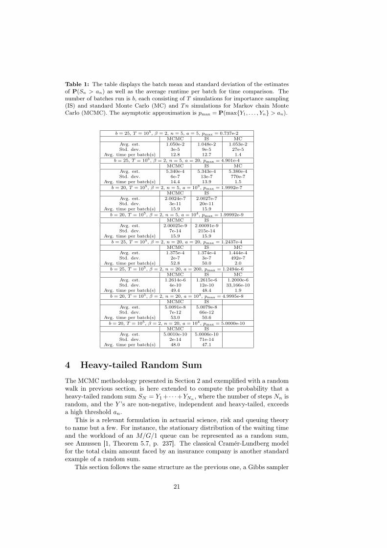
Table 1: The table displays the batch mean and standard deviation of the estimatesof P(Sn > an) as well as the average runtime per batch for time comparison. Thenumber of batches run is b, each consisting of T simulations for importance sampling(IS) and standard Monte Carlo (MC) and Tn simulations for Markov chain MonteCarlo (MCMC). The asymptotic approximation is pmax = P(max{Y1, . . . , Yn} > an).

b = 25, T = 105, β = 2, n = 5, a = 5, pmax = 0.737e-2MCMC IS MC

Avg. est. 1.050e-2 1.048e-2 1.053e-2Std. dev. 3e-5 9e-5 27e-5

Avg. time per batch(s) 12.8 12.7 1.4b = 25, T = 105, β = 2, n = 5, a = 20, pmax = 4.901e-4

MCMC IS MCAvg. est. 5.340e-4 5.343e-4 5.380e-4Std. dev. 6e-7 13e-7 770e-7


MCMC ISAvg. est. 2.0024e-7 2.0027e-7Std. dev. 3e-11 20e-11

Avg. time per batch(s) 15.9 15.9b = 20, T = 105, β = 2, n = 5, a = 104, pmax = 1.99992e-9





MCMC IS MCAvg. est. 1.2614e-6 1.2615e-6 1.2000e-6Std. dev. 4e-10 12e-10 33,166e-10





Avg. time per batch(s) 48.0 47.1

4 Heavy-tailed Random Sum

The MCMC methodology presented in Section 2 and exemplified with a randomwalk in previous section, is here extended to compute the probability that aheavy-tailed random sum SN = Y1+ · · ·+YNn

, where the number of steps Nn israndom, and the Y ’s are non-negative, independent and heavy-tailed, exceedsa high threshold an.

This is a relevant formulation in actuarial science, risk and queuing theoryto name but a few. For instance, the stationary distribution of the waiting timeand the workload of an M/G/1 queue can be represented as a random sum,see Amussen [1, Theorem 5.7, p. 237]. The classical Cramér-Lundberg modelfor the total claim amount faced by an insurance company is another standardexample of a random sum.

This section follows the same structure as the previous one, a Gibbs sampler

21

is presented for sampling from the conditional distribution P((Y1, . . . , YN ) ∈ · |SN > an). The resulting Markov chain is proved to be uniformly ergodic. Anestimator for (p(N))−1 of the form (2.1) is suggested with V (n) as the condi-tional distribution of (Y1, . . . , YN ) given max{Y1, . . . , YN} > an. The estimatoris proved to have vanishing normalised variance when the distribution of Y1belongs to the class of subexponential distributions. The section is concludedwith numerical experiments to illustrate the comparativeness with existing im-portance sampling algorithm and standard Monte Carlo.

4.1 A Gibbs sampler for computing P(SNn > an)

Let Y1, Y2, . . . be non-negative independent random variables with common dis-tribution FY and density fY . Let (N (n))n≥1 be integer valued random variablesindependent of Y1, Y2, . . . . Consider the random sum SN(n) = Y1 + · · · + YN(n)

and the problem of computing the probability

p(n) = P(SN(n) > an),

where an →∞ at an appropriate rate.Denote by Y

(n)the vector (N (n), Y1, . . . , YN(n))

>. The conditional distribu-

tion of Y(n)

given SN(n) > an is given by

P(N (n) = k, (Y1, . . . , Yk) ∈ · | SN(n) > an)

=P((Y1, . . . , Yk) ∈ · , Sk > an)P(N (n) = k)

p(n). (4.1)

A Gibbs sampler for sampling from the conditional distribution in (4.1) canbe constructed essentially as in Algorithm 3.1. The only additional difficulty isto update the random number of steps in an appropriate way. In the followingalgorithm a particular distribution for updating the number of steps is proposed.To ease the notation the superscript n is suppressed in the description of thealgorithm.

Algorithm 4.1. To initiate, draw N0 from P(N ∈ ·) and Y0,1, . . . , Y0,N0such

that Y0,1 + · · · + Y0,N0> an. Each iteration of the algorithm consists of the

following steps. Suppose Yt = (kt, yt,1, . . . , yt,kt) with yt,1 + · · · + yt,kt > an.Write k∗t = min{j : yt,1 + · · ·+ yt,j > an}.

1. Sample the number of steps Nt+1 from the distribution

p(kt+1 | k∗t ) =P(N = kt+1)I{kt+1 ≥ k∗t }

P (N ≥ k∗t ).

If Nt+1 > Nt, sample Yt+1,kt+1, . . . , Yt+1,Nt+1independently from FY and

put Y(1)t = (Yt,1, . . . , Yt,kt , Yt+1,kt+1, . . . , Yt+1,Nt+1

).

2. Proceed by updating all the individual steps as follows:

(a) Draw j1, . . . , jNt+1from {1, . . . , Nt+1} without replacement and pro-

ceed by updating the components of Y(1)t in the order thus obtained.

(b) For each k = 1, . . . , Nt+1, repeat the following.

22

i. Let j = jk be the index to be updated and write

Y(1)t,−j = (Y

(1)t,1 , . . . , Y

(1)t,j−1, Y

(1)t,j+1, . . . , Y

(1)t,Nt+1

).

Sample Y (2)t,j from the conditional distribution of Y given that

the sum exceeds the threshold. That is,

P(Y(2)t,j ∈ · | Y

(1)t,−j) = P

(Y ∈ · | Y +

∑k 6=j

Y(1)t,k > an

).

ii. Put Y(2)t = (Y

(1)t,1 , . . . , Y

(1)t,j−1, Y

(2)t,j , Y

(1)t,j+1, . . . , Y

(1)t,Nt+1

)>.

(c) Draw a random permutation π of the numbers {1, . . . , Nt+1} from theuniform distribution and put Yt+1 = (Nt+1, Y

(2)t,π(1), . . . , Y

(2)t,π(Nt+1)

).

Iterate until the entire Markov Chain (Yt)T−1t=0 is constructed.

Proposition 4.2. The Markov chain (Yt)t≥0 generated by Algorithm 4.1 hasthe conditional distribution P((N,Y1, . . . , YN ) ∈ · | Y1 + . . . YN > an) as itsinvariant distribution.

Proof. The only essential difference from Algorithm 3.1 is the first step of thealgorithm, where the number of steps and possibly the additional steps areupdated. Therefore, it is sufficient to prove that the first step of the algorithmpreserves stationarity. The transition probability of the first step, starting froma state (kt, yt,1, . . . , yt,kt) with k∗t = min{j : yt,1 + · · · + yt,j > an}, can bewritten as follows.

P (1)(kt, yt,1, . . . , yt,kt ; kt+1, A1 × · · · ×Akt+1)

= P(Nt+1 = kt+1, (Yt,1, . . . , Yt,kt+1) ∈ A1 × · · · ×Akt+1

| Nt = kt, Yt,1 = yt,1, . . . , Yt,kt = yt,kt)

=

{p(kt+1 | k∗t )

∏kt+1

k=1 I{yt,k ∈ Ak}, kt+1 ≤ kt,p(kt+1 | k∗t )

∏ktk=1 I{yt,k ∈ Ak}

∏kt+1

k=kt+1 FY (Ak), kt+1 > kt.

Consider the stationary probability of a set of the form {kt+1} × A1 × · · · ×Akt+1

. With π denoting the conditional distribution P((N,Y1, . . . , YN ) ∈ · |Y1 + . . . YN > an), it holds that

Eπ[P(1)(Nt, Yt,1, . . . , Yt,Nt

; kt+1, A1 × · · · ×Akt+1)]

=1

P(SN > an)E[P (1)(N,Y1, . . . , YN ; kt+1, A1 × · · · ×Akt+1

)I{SN > an}]

By conditioning onN and using independence ofN and Y1, Y2, . . . the expressionin the last display equals

1

P(SN > an)

∞∑kt=1

P(N = kt)

×E[P (1)(kt, Y1, . . . , Ykt ; kt+1, A1 × · · · ×Akt+1)I{Skt > an}

].

23

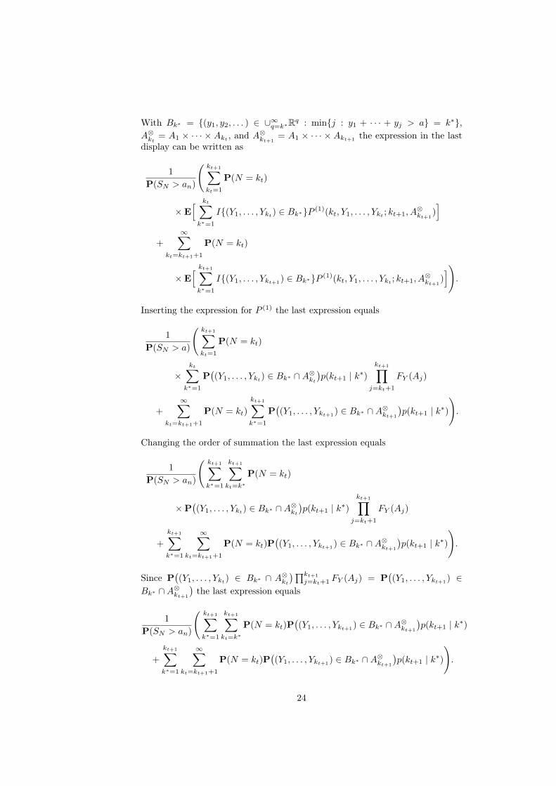
With Bk∗ = {(y1, y2, . . . ) ∈ ∪∞q=k∗Rq : min{j : y1 + · · · + yj > a} = k∗},A⊗kt = A1 × · · · × Akt , and A⊗kt+1

= A1 × · · · × Akt+1 the expression in the lastdisplay can be written as

1

P(SN > an)

(kt+1∑kt=1

P(N = kt)

×E[ kt∑k∗=1

I{(Y1, . . . , Ykt) ∈ Bk∗}P (1)(kt, Y1, . . . , Ykt ; kt+1, A⊗kt+1

)]

+

∞∑kt=kt+1+1

P(N = kt)

×E[ kt+1∑k∗=1

I{(Y1, . . . , Ykt+1) ∈ Bk∗}P (1)(kt, Y1, . . . , Ykt ; kt+1, A

⊗kt+1

)]).

Inserting the expression for P (1) the last expression equals

1

P(SN > a)

(kt+1∑kt=1

P(N = kt)

×kt∑

k∗=1

P((Y1, . . . , Ykt) ∈ Bk∗ ∩A⊗kt

)p(kt+1 | k∗)

kt+1∏j=kt+1

FY (Aj)

+

∞∑kt=kt+1+1

P(N = kt)

kt+1∑k∗=1

P((Y1, . . . , Ykt+1) ∈ Bk∗ ∩A⊗kt+1

)p(kt+1 | k∗)

).

Changing the order of summation the last expression equals

1

P(SN > an)

(kt+1∑k∗=1

kt+1∑kt=k∗

P(N = kt)

×P((Y1, . . . , Ykt) ∈ Bk∗ ∩A⊗kt

)p(kt+1 | k∗)

kt+1∏j=kt+1

FY (Aj)

+

kt+1∑k∗=1

∞∑kt=kt+1+1

P(N = kt)P((Y1, . . . , Ykt+1

) ∈ Bk∗ ∩A⊗kt+1

)p(kt+1 | k∗)

).

Since P((Y1, . . . , Ykt) ∈ Bk∗ ∩ A⊗kt

)∏kt+1

j=kt+1 FY (Aj) = P((Y1, . . . , Ykt+1

) ∈Bk∗ ∩A⊗kt+1

)the last expression equals

1

P(SN > an)

(kt+1∑k∗=1

kt+1∑kt=k∗

P(N = kt)P((Y1, . . . , Ykt+1

) ∈ Bk∗ ∩A⊗kt+1

)p(kt+1 | k∗)

+

kt+1∑k∗=1

∞∑kt=kt+1+1

P(N = kt)P((Y1, . . . , Ykt+1

) ∈ Bk∗ ∩A⊗kt+1

)p(kt+1 | k∗)

).

24

Summing over kt the last expression equals

1

P(SN > an)

(kt+1∑k∗=1

P((Y1, . . . , Ykt+1

) ∈ Bk∗ ∩A⊗kt+1

)p(kt+1 | k∗)P(k∗ ≤ N ≤ kt+1)

+

kt+1∑k∗=1

P((Y1, . . . , Ykt+1) ∈ Bk∗ ∩A⊗kt+1

)p(kt+1 | k∗)P(N ≥ kt+1 + 1)

).

From the definition of p(kt+1 | k∗) it follows that the last expression equals

1

P(SN > an)

kt+1∑k∗=1

P((Y1, . . . , Ykt+1) ∈ Bk∗ ∩A⊗kt+1

)p(kt+1 | k∗)P (N ≥ k∗)

=1

P(SN > an)

kt+1∑k∗=1

P((Y1, . . . , Ykt+1) ∈ Bk∗ ∩A⊗kt+1

)P (N = kt+1)

=1

P(SN > an)P((Y1, . . . , Ykt+1

) ∈ A⊗kt+1

)P (N = kt+1)

= P(N = kt+1, (Y1, . . . , Ykt+1

) ∈ A⊗kt+1| Y1 + · · ·+ YN > an

),

which is the desired invariant distribution. This completes the proof.

Proposition 4.3. The Markov chain (Yt)t≥0 generated by Algorithm 4.1 isuniformly ergodic. In particular, it satisfies the following minorisation condi-tion: there exists δ > 0 such that

P(Y1 ∈ B | Y0 = y) ≥ δP((N,Y1, . . . , YN ) ∈ B | Y1 + · · ·+ YN > an),

for all y ∈ A = ∪k≥1{(k, y1, . . . , yk) : y1 + · · · + yk > an} and all Borel setsB ⊂ A.

The proof requires only a minor modification from the non-random case,Proposition 3.4, and is therefore omitted.

4.2 Constructing an efficient estimatorNow consider the distributional assumptions and the design of V (n). The mainfocus is on the rare event properties of the estimator and therefore the largedeviation parameter n will be suppressed to ease notation. Let the distributionof the number of steps P(N (n) ∈ ·) to depend on n. By a similar reasoning as inthe case of non-random number of steps the following assumption are imposed:the variables N (n), Y1, Y2, . . . and the numbers an are such that

limn→∞

P(Y1 + · · ·+ YN(n) > an)

P(MN(n) > an)= 1, (4.2)

where Mk = max{Y1, . . . , Yk}. Note that the denominator can be expressed as

P(MN(n) > an) =

∞∑k=1

P(Mk > an)P(N (n) = k)

=

∞∑k=1

[1− FY (an)k]P(N (n) = k)

= 1− gN(n)(FY (an)),

25

where gN(n)(t) = E[tN(n)

] is the generating function of N (n). Sufficient con-ditions for (4.2) to hold are given in [37], Theorem 3.1. For instance, if FY isregularly varying at∞ with index β > 1 and N (n) has Poisson distribution withmean λn →∞, as n→∞, then (4.2) holds with an = aλn, for a > 0.

Similarly to the non-random setting a good candidate for V (n) is the condi-tional distribution,

V (n)(·) = P(Y(n) ∈ · |MN(n) > an).

Then V (n) has a known density with respect to F (n)(·) = P(Y(n) ∈ ·) given by

dV (n)

dF (n)(k, y1, . . . , yk) =

1

P(MN(n) > an)I{(y1, . . . , yk) : ∨kj=1yj > an}

=1

1− gN(n)(FY (an))I{(y1, . . . , yk) : ∨kj=1yj > an}.

The estimator of q(n) = P(Sn > an)−1 is given by

q̂(n)T =

1

T

T−1∑t=0

dV (n)

dF (n)(Y

(n)

t ) =1

gN(n)(FY (an))· 1T

T−1∑t=0

I{∨Ntj=1Yt,j > an}, (4.3)

where (Y(n)

t )t≥0 is generated by Algorithm 4.1.

Theorem 4.4. Suppose (4.2) holds. The estimator q̂(n)T in (4.3) has vanishingnormalised variance. That is,

limn→∞

(p(n))2 Varπn(q̂

(n)T ) = 0,

where πn denotes the conditional distribution P(Y(n) ∈ · | SN(n) > an).

Remark 4.5. Because the distribution of N (n) may depend on n Theorem 4.4covers a wider range of settings for random sums than those studied in [16, 9]where the authors present provably efficient importance sampling algorithms.

Proof. Since p(n) = P(SN(n) > an) and

u(n)(k, y1, . . . , yk) =I{∨kj=1yj > an}P(MN(n) > an)

,

it follows that

[p(n)]2 Varπn(u(n)(Y

(n)))

=P(SN(n) > an)

2

P(MN(n) > an)2Varπn

(I{∨N(n)

j=1 Yj > an})

=P(SN(n) > an)

2

P(MN(n) > an)2P(MN(n) > an | SN(n) > an)P(MN(n) ≤ an | SN(n) > an)

=P(SN(n) > an)

P(MN(n) > an)

(1− P(MN(n) > an)

P(SN(n) > an)

)→ 0,

by (4.2). This completes the proof.

26

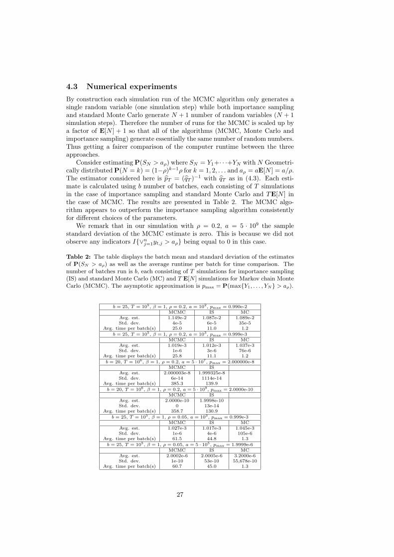
4.3 Numerical experimentsBy construction each simulation run of the MCMC algorithm only generates asingle random variable (one simulation step) while both importance samplingand standard Monte Carlo generate N + 1 number of random variables (N + 1simulation steps). Therefore the number of runs for the MCMC is scaled up bya factor of E[N ] + 1 so that all of the algorithms (MCMC, Monte Carlo andimportance sampling) generate essentially the same number of random numbers.Thus getting a fairer comparison of the computer runtime between the threeapproaches.

Consider estimatingP(SN > aρ) where SN = Y1+· · ·+YN withN Geometri-cally distributedP(N = k) = (1−ρ)k−1ρ for k = 1, 2, . . . and aρ = aE[N ] = a/ρ.The estimator considered here is p̂T = (q̂T )

−1 with q̂T as in (4.3). Each esti-mate is calculated using b number of batches, each consisting of T simulationsin the case of importance sampling and standard Monte Carlo and TE[N ] inthe case of MCMC. The results are presented in Table 2. The MCMC algo-rithm appears to outperform the importance sampling algorithm consistentlyfor different choices of the parameters.

We remark that in our simulation with ρ = 0.2, a = 5 · 109 the samplestandard deviation of the MCMC estimate is zero. This is because we did notobserve any indicators I{∨nj=1yt,j > aρ} being equal to 0 in this case.

Table 2: The table displays the batch mean and standard deviation of the estimatesof P(SN > aρ) as well as the average runtime per batch for time comparison. Thenumber of batches run is b, each consisting of T simulations for importance sampling(IS) and standard Monte Carlo (MC) and T E[N ] simulations for Markov chain MonteCarlo (MCMC). The asymptotic approximation is pmax = P(max{Y1, . . . , YN} > aρ).

b = 25, T = 105, β = 1, ρ = 0.2, a = 102, pmax = 0.990e-2MCMC IS MC


Avg. time per batch(s) 25.0 11.0 1.2b = 25, T = 105, β = 1, ρ = 0.2, a = 103, pmax = 0.999e-3


Avg. time per batch(s) 25.8 11.1 1.2b = 20, T = 106, β = 1, ρ = 0.2, a = 5 · 107, pmax = 2.000000e-8


Avg. time per batch(s) 385.3 139.9b = 20, T = 106, β = 1, ρ = 0.2, a = 5 · 109, pmax = 2.0000e-10

MCMC ISAvg. est. 2.0000e-10 1.9998e-10Std. dev. 0 13e-14

Avg. time per batch(s) 358.7 130.9b = 25, T = 105, β = 1, ρ = 0.05, a = 103, pmax = 0.999e-3


Avg. time per batch(s) 61.5 44.8 1.3b = 25, T = 105, β = 1, ρ = 0.05, a = 5 · 105, pmax = 1.9999e-6

MCMC IS MCAvg. est. 2.0002e-6 2.0005e-6 3.2000e-6Std. dev. 1e-10 53e-10 55,678e-10

Avg. time per batch(s) 60.7 45.0 1.3

27

5 Stochastic Recurrence Equations

The MCMC methodology presented in Section 2 is here applied to compute theprobability that a solution Xm to a recurrence equation Xm = AmXm−1 +Bm,where the innovations B are regularly varying with index α and E[Aα+ε] < ∞for some ε > 0, exceeds a high threshold cn. This problem has been consideredusing importance sampling scheme by Hult, Blanchet and Leder in [27].

In this section a Gibbs sampler is presented for sampling from the conditionaldistribution P(A1, . . . , Am, B1, . . . , Bm | Xm > cn). The resulting Markov chainis proved to be uniformly ergodic. An estimator for (p(n))−1 of the form (2.1) issuggested with V (n) as the conditional distribution of (A1, . . . , Am, B1, . . . , Bm)given {Ak > a, ∀k} ∩ {∃!j : Bja

m−j > cn}. The estimator is proved to havevanishing normalised variance under the probabilistic assumptions mentionedabove. The proof is elementary and is completed in a few lines. The sectionis concluded with numerical experiments to illustrate the comparativeness withexisting importance sampling algorithm and standard Monte Carlo.

5.1 A Gibbs sampler for computing P(Xm > cn)

Fix m and let A = (A2, . . . , Am) and B = (B1, . . . , Bm) be independent se-quences of independent and identically distributed random variables. Let A bea generic random variable for an element of the sequence A and likewise B foran element of the sequence B.

Consider the solution (Xk)mk=0 to the stochastic recurrence equation

Xk = AkXk−1 +Bk, for k = 1, . . . ,m,X0 = 0.

The solution (Xk)mk=0 can be written as a randomly weighted random walk

Xk = Bk +AkBk−1 + · · ·+AkAk−1 · · ·A2B1 +Ak · · ·A1x0, k = 1, . . . ,m.(5.1)

Our interest is in the problem of computing p(n) = P(Xm > cn), wherecn →∞. To this end we will propose a Gibbs sampler that produces a Markovchain with the conditional distribution

F (m)cn (·) = P

((A,B) ∈ · | Xm > cn

)(5.2)

as its invariant distribution. In addition we will suggest a choice of the proba-bility distribution V (n) with good asymptotic properties.

The Markov chain (At,Bt)t≥0 is constructed by the following algorithm,where the elements are updated sequentially in such a way that the weightedrandom walk exceeds the threshold after each individual update. Formally thealgorithm is given as follows. An empty product, such as

∏mj=m+1Aj , is inter-

preted as 1.

Algorithm 5.1. Start with initial state (A(m)0 ,B(m)

0 ) = (A0,2, . . . , A0,m, B0,1, . . . , B0,m)

where X(m)0 = B0,m +

∑m−1i=1 B0,i

∏mj=i+1A0,j > cn. Given (A(m)

t ,B(m)t ), for

some t = 0, 1, . . ., the next state (A(m)t+1,B

(m)t+1) is sampled as follows:

28

1. Draw a randomized ordering j1, . . . , j2m of {1, . . . , 2m} and proceed up-dating (A(m)

t ,B(m)t ) in the order thus obtained.

2. For l = 1, . . . , 2m, set k = jl and do the following:

i. If k ∈ {1, . . . ,m} then At,k is to be updated. Sample A′ from theconditional distribution

P(A′ ∈ · | A′ > s),

where

s = max

{cn −

∑mi=k Bt,i

∏mj=i+1At,j∑k−1

i=1 Bt,i∏mj=i+1, 6=k At,j

, 0

}.

PutA(m)t+1 = (At,1, . . . , At,k−1, A

′, At,k+1, . . . , At,m) andB(m)t+1 = B(m)

t .ii. If k ∈ {m + 1, . . . , 2m} then Bt,(k−m) is to be updated. Sample B′

from the conditional distribution

P(B′ ∈ · | B′ > s),

where

s = max

{cn −

∑mi=1,6=(k−m)Bt,i

∏mj=i+1At,j

At,m · · ·At,(k−m)+1, 0

}.

PutA(m)t+1 = A(m)

t andB(m)t+1 = (Bt,1, . . . , Bt,(k−m)−1, B

′, Bt,(k−m)+1, . . . , Bt,m).

Iterate steps 1 and 2 until the entire Markov chain (A(m)t ,B(m)

t )T−1t=0 is con-structed.

The Markov chain (A(m)t ,B(m)

t )t≥0 constructed by Algorithm 5.1 has F (m)cn

as its invariant probability distribution.

Proposition 5.2. The Markov chain (A(m)t ,B(m)

t )t≥0 generated by Algorithm5.1, has the conditional distribution F (m)

cn as its invariant distribution.

Proof. Note that it is sufficient to show that each updating step (Step 2i and2ii in the Algorithm) preserves stationarity.

Consider the updating steps (Step 2i and 2ii). Let m be given and setPAk (a(m),b(m), ·) and PBk (a(m),b(m), ·) to be the transition probability of theMarkov chain (A(m)

t ,B(m)t )t≥0 where the kth element of A(m)

t and B(m)t is

updated, respectively. Let

R ={(A1, . . . , Am, B1, . . . , Bm) | Xm > cn},

and observe that if Ak is to be updated conditioned on Xm > cn then

Ak >cn −

∑mi=k Bt,i

∏mj=i+1At,j∑k−1

i=1 Bt,i∏mj=i+1,6=k At,j

=: sAk,

and similarly, if Bk is to be updated conditioned on Xm > cn then

Bk >cn −

∑mi=1,6=(k−m)Bt,i

∏mj=i+1At,j

At,m · · ·At,(k−m)+1=: sBk

.

29

To prove that stationarity is preserved under updating via Step 2i it is sufficientto show that for arbitrary k ∈ {1, . . . ,m} and D1×· · ·×Dm×E1×· · ·×Em ⊂ Rthen it holds that

F (m)cn (D1 × · · · ×Dm × E1 × · · · × Em)

= EF

(m)cn

[PAk (A1, . . . , Am, B1, . . . , Bm, D1 × . . .×Dm × E1 × . . .× Em)

].

(5.3)

Similarly to prove that stationarity is preserved under updating via Step 2ii itis sufficient to show

F (m)cn (D1 × · · · ×Dm × E1 × · · · × Em)

= EF

(m)cn

[PBk (A1, . . . , Am, B1, . . . , Bm, D1 × · · · ×Dm × E1 × · · · × Em)

].

(5.4)

The following computation shows that (5.3) holds.

F (m)cn (D1 × · · · ×Dm × E1 × · · · × Em)

= EF

(m)cn

[ m∏j=1

I{Aj ∈ Dj}m∏i=1

I{Bi ∈ Ei}]

=E[I{Ak ∈ Dk}I{Xm > cn} ·

∏mj=1,6=k I{Aj ∈ Dj}

∏mi=1 I{Bi ∈ Ei}

]P(Xm > cn)

=E[E[I{Ak∈Dk}|Ak>sAk

,A−k,B]

P(Ak>sAk) ·



]P(Xm > cn)

=E[PAk (A,B, D1 × · · · ×Dm × E1 × · · · × Em) ·



]P(Xm > cn)

= E[PAk (A,B, D1 × · · · ×Dm × E1 × · · · × Em) | Xm > cn

]= E

F(m)cn

[PAk (A,B, D1 × · · · ×Dm × E1 × · · · × Em)

],

with the conventional notation A−k = (A1, . . . , Ak−1, Ak+1, . . . , Am).The proof is completed by showing that (5.4) holds with similar computation

as above.

The Markov chain (A(m)t ,B(m)

t )t≥0 constructed by Algorithm 5.1 is uni-formly ergodic, thus ensuring large-sample efficiency.

Proposition 5.3. For any m ≥ 1, the Markov chain (A(m)t ,B(m)

t )t≥0 is uni-formly ergodic.

Proof. Let m ≥ 1 be given and set

R ={(A1, . . . , Am, B1, . . . , Bm) | Xm > cn}.

Uniform ergodicity follows from the minorization condition (see Nummelin [44]): there exists a probability measure ν, δ > 0 and t0 ∈ N such that

P((A(m)

t0 ,B(m)t0 ) ∈ D × E | (A(m)

0 ,B(m)0 ) = (a,b)

)≥ δν(D × E),

30

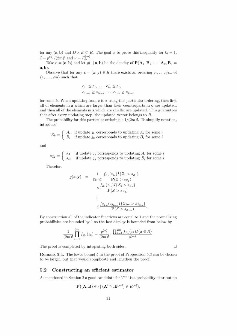
for any (a,b) and D × E ⊂ R. The goal is to prove this inequality for t0 = 1,δ = p(n)/(2m)! and ν = F

(m)cn .

Take c = (a,b) and let g(· | a,b) be the density of P(A1,B1 ∈ · | A0,B0 =a,b).

Observe that for any z = (x,y) ∈ R there exists an ordering j1, . . . , j2m of{1, . . . , 2m} such that

cj1 ≤ zj1 , . . . , cjk ≤ zjkcjk+1

≥ zjk+1, . . . , cj2m ≥ zj2m ,

for some k. When updating from c to z using this particular ordering, then firstall of elements in z which are larger than their counterparts in c are updated,and then all of the elements in z which are smaller are updated. This guaranteesthat after every updating step, the updated vector belongs to R.

The probability for this particular ordering is 1/(2m)!. To simplify notation,introduce

Zk =

{Ai if update jk corresponds to updating Ai for some iBi if update jk corresponds to updating Bi for some i

and

sZk=

{sAi if update jk corresponds to updating Ai for some isBi if update jk corresponds to updating Bi for some i

Therefore

g(x,y) =1

(2m)!

fZ1(zj1)I{Z1 > sZ1}P(Z > sZ1

)

×fZ2(zj2)I{Z2 > sZ2

}P(Z > sZ2)

...

×fZ2m(zj2m)I{Z2m > sZ2m

}P(Z > sZ2m

).

By construction all of the indicator functions are equal to 1 and the normalizingprobabilities are bounded by 1 so the last display is bounded from below by

1

(2m)!

2m∏k=1

fZk(zk) =

p(n)

(2m)!·∏2mk=1 fZk

(zk)I{z ∈ R}p(m)

.

The proof is completed by integrating both sides.

Remark 5.4. The lower bound δ in the proof of Proposition 5.3 can be chosento be larger, but that would complicate and lengthen the proof.

5.2 Constructing an efficient estimatorAs mentioned in Section 2 a good candidate for V (n) is a probability distribution

P((A,B) ∈ · | (A(m),B(m)) ∈ R(n)

),

31

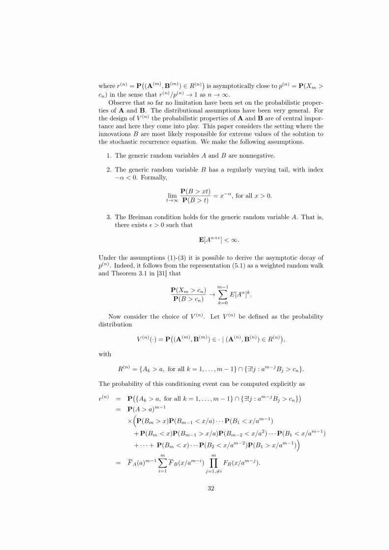
where r(n) = P((A(m),B(m)) ∈ R(n)

)is asymptotically close to p(n) = P(Xm >

cn) in the sense that r(n)/p(n) → 1 as n→∞.Observe that so far no limitation have been set on the probabilistic proper-

ties of A and B. The distributional assumptions have been very general. Forthe design of V (n) the probabilistic properties of A and B are of central impor-tance and here they come into play. This paper considers the setting where theinnovations B are most likely responsible for extreme values of the solution tothe stochastic recurrence equation. We make the following assumptions.

1. The generic random variables A and B are nonnegative.

2. The generic random variable B has a regularly varying tail, with index−α < 0. Formally,

limt→∞

P(B > xt)

P(B > t)= x−α, for all x > 0.

3. The Breiman condition holds for the generic random variable A. That is,there exists ε > 0 such that

E[Aα+ε] <∞.

Under the assumptions (1)-(3) it is possible to derive the asymptotic decay ofp(n). Indeed, it follows from the representation (5.1) as a weighted random walkand Theorem 3.1 in [31] that

P(Xm > cn)

P(B > cn)→

m−1∑k=0

E[Aα]k.

Now consider the choice of V (n). Let V (n) be defined as the probabilitydistribution

V (n)(·) = P((A(m),B(m)) ∈ · | (A(n),B(n)) ∈ R(n)

),

with

R(n) = {Ak > a, for all k = 1, . . . ,m− 1} ∩ {∃!j : am−jBj > cn}.

The probability of this conditioning event can be computed explicitly as

r(n) = P({Ak > a, for all k = 1, . . . ,m− 1} ∩ {∃!j : am−jBj > cn}

)= P(A > a)m−1

×(P(Bm > x)P(Bm−1 < x/a) · · ·P(B1 < x/am−1)

+P(Bm < x)P(Bm−1 > x/a)P(Bm−2 < x/a2) · · ·P(B1 < x/am−1)

+ · · ·+ P(Bm < x) · · ·P(B2 < x/am−2)P(B1 > x/am−1))

= FA(a)m−1

m∑i=1

FB(x/am−i)

m∏j=1,6=i

FB(x/am−j).

32

From the regular variation property of the distribution of B, assumption (2),it follows that

r(n) ∼ FA(a)m−1FB(cn)

{1 + aα + (aα)2 + · · ·+ (aα)m−1

}as n→∞.

A convenient choice of the level a = an is such that r(n)/p(n) → 1, as n → ∞.That is, a may be chosen as the solution to

FA(a)m−1

m−1∑k=0

akα =

m−1∑k=0

E[Aα]k.

The distribution V (n) has a known density with respect to F (·) = P((A(m),B(m)) ∈

·) given bydV (n)

dF (·)(a,b) =

1

r(n)I{(a,b) ∈ Rm

}.

Thus the MCMC estimator q̂(n)T of 1/p(n) is given by

q̂(n)T =

1

r(n)1

T

T−1∑t=0

I{(A(m)

t ,B(m)t ) ∈ R(n)

}, (5.5)

where (At,Bt)T−1t=0 is generated via Algorithm 5.1. Observe that the estimator

first factor of the estimator q̂(n)T may be interpreted as the asymptotic approxi-mation 1/r(n) multiplied by a stochastic correction factor.

Theorem 5.5. The estimator q(n)T given by 5.5 has vanishing normalized vari-ance for estimating 1/p(n),

limn→∞

(p(n)

)2VarFcn

(q̂(n)T )→ 0.

Proof. With u(n)(a,b) = 1r(n) I{(a,b) ∈ R} it follows from assumptions 1-3

made above that

(p(n))2 VarF

(m)cn

( 1

r(n)I{(a,b) ∈ R}

)=

(p(n))2

(r(n))2Var

F(m)cn

(I{(a,b) ∈ R}

)=

(p(n))2

(r(n))2P(I{(a,b) ∈ R} | Xm > cn

)P(I{(a,b) /∈ R} | Xm > cn

)=p(n)

r(n)P(1− r(n)

p(n)

)→ 0.

This completes the proof.

5.3 Numerical experiments

Theorem 5.5 of this paper proves that q̂(n)T is an efficient estimator of 1/p(n).Most existing algorithms however design an efficient estimator p̂(n)T of p(n), sofor comparison reasons the numerical experiments are based on (q̂

(n)T )−1.

33

By construction each simulation run of the MCMC algorithm only generatesa single random variable (one simulation step) while both importance samplingand standard Monte Carlo generate 2m number of random variables (2m sim-ulation steps). Therefore the number of runs for the MCMC is scaled up bya factor of 2m so that all of the algorithms (MCMC, Monte Carlo and im-portance sampling) generate essentially the same number of random numbers.Thus getting a fairer comparison of the computer runtime between the threeapproaches.

Consider estimating P(Xn > cn) where Xn is a solution to the recurrenceequation Xn = AnXn−1 + Bn with X0 = 0. The innovation B is a Paretodistributed variable with index α while the A is exponentially distributed withintensity λ. Each estimate is calculated using b number of batches, each con-sisting of T simulations in the case of importance sampling and standard MonteCarlo and 2nT in the case of MCMC. The results are presented in Table 3.

Table 3: The table displays the batch mean and standard deviation of the estimatesof P(Xn > c) as well as the average runtime per batch for time comparison. Thenumber of batches run is b, each consisting of T simulations for importance sampling(IS) and standard Monte Carlo (MC) and T 2n simulations for Markov chain MonteCarlo (MCMC).

b = 25, T = 105, n = 4, c = 10, α = 2, λ = 3MCMC IS MC


Avg. time per batch(s) 35 36 2b = 25, T = 105, n = 4, c = 102, α = 2, λ = 3

MCMC IS MCAvg. est. 1.298e-4 1.278e-4 1.360e-4Std. dev. 7e-6 1e-6 35e-6b = 25, T = 105, n = 4, c = 103, α = 2, λ = 3

MCMC IS MCAvg. est. 1.149e-6 1.284e-6 2.000e-6Std. dev. 36e-8 7e-8 408e-8b = 25, T = 105, n = 5, c = 2, α = 5, λ = 3

34

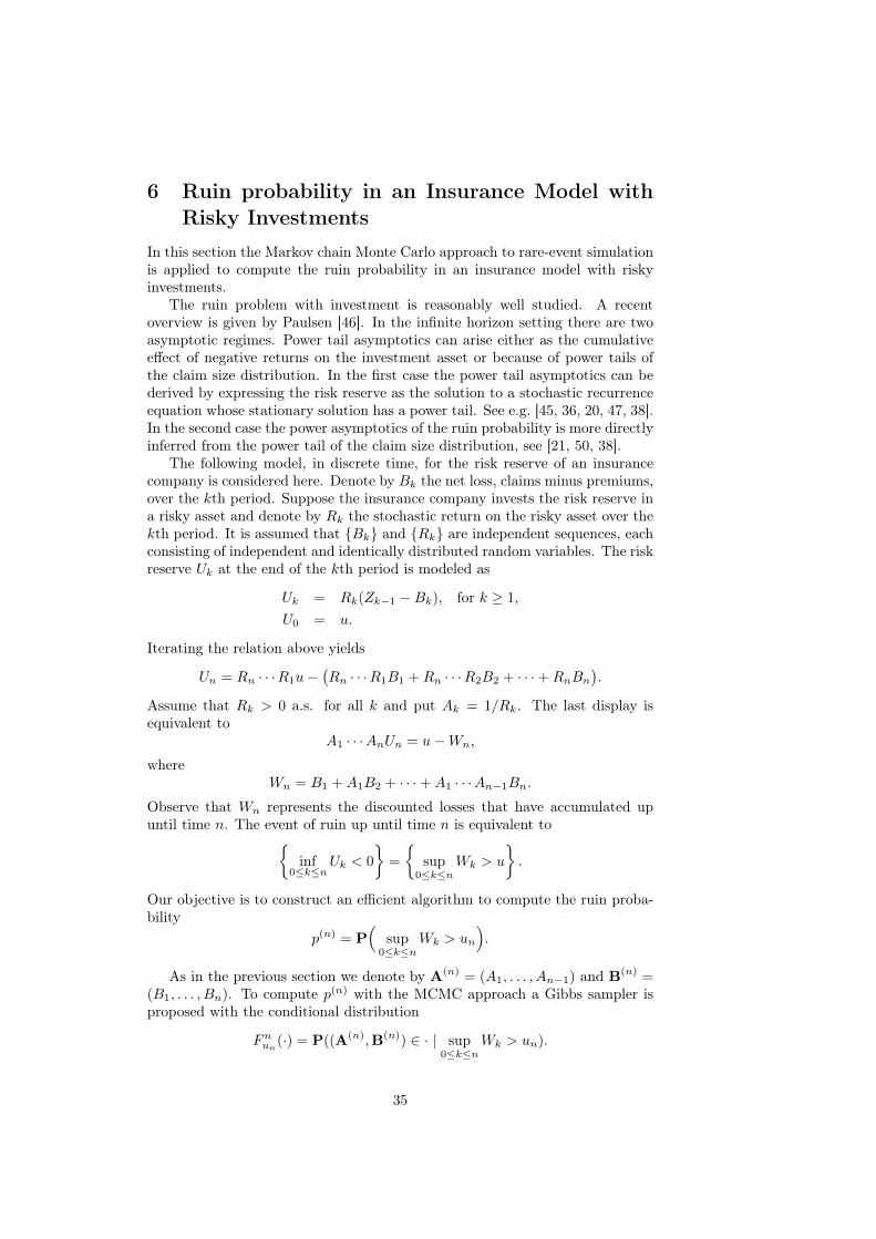
6 Ruin probability in an Insurance Model withRisky Investments

In this section the Markov chain Monte Carlo approach to rare-event simulationis applied to compute the ruin probability in an insurance model with riskyinvestments.

The ruin problem with investment is reasonably well studied. A recentoverview is given by Paulsen [46]. In the infinite horizon setting there are twoasymptotic regimes. Power tail asymptotics can arise either as the cumulativeeffect of negative returns on the investment asset or because of power tails ofthe claim size distribution. In the first case the power tail asymptotics can bederived by expressing the risk reserve as the solution to a stochastic recurrenceequation whose stationary solution has a power tail. See e.g. [45, 36, 20, 47, 38].In the second case the power asymptotics of the ruin probability is more directlyinferred from the power tail of the claim size distribution, see [21, 50, 38].

The following model, in discrete time, for the risk reserve of an insurancecompany is considered here. Denote by Bk the net loss, claims minus premiums,over the kth period. Suppose the insurance company invests the risk reserve ina risky asset and denote by Rk the stochastic return on the risky asset over thekth period. It is assumed that {Bk} and {Rk} are independent sequences, eachconsisting of independent and identically distributed random variables. The riskreserve Uk at the end of the kth period is modeled as

Uk = Rk(Zk−1 −Bk), for k ≥ 1,U0 = u.

Iterating the relation above yields

Un = Rn · · ·R1u−(Rn · · ·R1B1 +Rn · · ·R2B2 + · · ·+RnBn

).

Assume that Rk > 0 a.s. for all k and put Ak = 1/Rk. The last display isequivalent to

A1 · · ·AnUn = u−Wn,

whereWn = B1 +A1B2 + · · ·+A1 · · ·An−1Bn.

Observe that Wn represents the discounted losses that have accumulated upuntil time n. The event of ruin up until time n is equivalent to{

inf0≤k≤n

Uk < 0

}=

{sup

0≤k≤nWk > u

}.

Our objective is to construct an efficient algorithm to compute the ruin proba-bility

p(n) = P(

sup0≤k≤n

Wk > un

).

As in the previous section we denote by A(n) = (A1, . . . , An−1) and B(n) =(B1, . . . , Bn). To compute p(n) with the MCMC approach a Gibbs sampler isproposed with the conditional distribution

Fnun(·) = P((A(n),B(n)) ∈ · | sup

0≤k≤nWk > un).

35

6.1 A Gibbs sampler for computing the ruin probabilityThe Gibbs sampler is constructed similarly as in Section 5 with the differencethat the conditioning event is {sup0≤k≤nWk > un} instead of {Xm > cn}.

Algorithm 6.1. Start with initial state (A(n)0 ,B(n)

0 ) = (A0,1, . . . , A0,n, B0,1, . . . , B0,n)

where X(n)0 > un. Given (A(n)

t ,B(n)t ), for some t = 0, 1, . . ., the next state

(A(n)t+1,B

(n)t+1) is sampled as follows:

1. Draw a randomized ordering j1, . . . , j2n of {1, . . . , 2n} and proceed updat-ing (A(n)

t ,B(n)t ) in the order thus obtained.

2. For m = 1, . . . , 2n, set k = jm and do the following:

i. If k ∈ {1, . . . , n} then At,k is to be updated. Sample A′ from theconditional distribution

P(A′ ∈ · | A′ > s),

where

s = min1≤k≤n

{un −

∑ki=1Bt,i

∏k−1j=1 At,j∑n

i=k+1Bt,i∏i−1j=1,6=k At,j

}.

Put A(n)t+1 = (At,1, . . . , At,k−1, A

′, At,k+1, . . . , At,n) and B(n)t+1 = B(n)

t .

ii. If k ∈ {n + 1, . . . , 2n} then Bt,(k−n) is to be updated. Sample B′from the conditional distribution

P(B′ ∈ · | B′ > s),

where

s = min1≤(k−n)≤n

{un −

∑ni=1,6=(k−n)Bt,i

∏i−1j=1At,j∏(k−n)−1

j=1 At,j

}.

PutA(n)t+1 = A(n)

t andB(n)t+1 = (Bt,1, . . . , Bt,(k−n)−1, B

′, Bt,(k−n)+1, . . . , Bt,n).

Iterate steps 1 and 2 until the entire Markov chain (A(n)t ,B(n)

t )T−1t=0 is con-structed.

Proposition 6.2. The Markov chain (A(n)t ,B(n)

t )t≥0 generated by Algorithm6.1, has the conditional distribution F

(n)un as its invariant distribution and is

uniformly ergodic.

The proof of the above result is essentially identical to the proofs of Propo-sition 5.2 and 5.3 is therefore omitted.

6.2 Constructing an efficient estimator of the reciprocalruin probability

As mentioned in Section 2 a good candidate for V (n) is a probability distribution

P((A,B) ∈ · | (A(n),B(n)) ∈ R(n)

),

36

where r(n) = P((A(n),B(n)) ∈ R(n)

)is asymptotically close to p(n) in the sense

that r(n)/p(n) → 1 as n→∞.Observe that, apart from the independence assumptions, the distributional

assumptions on B and R have been completely general. For the design of V (n)

the probabilistic properties of B and R are of central importance and here theycome into play. This paper considers the setting where large claims are mostlikely responsible for ruin. We make the following assumptions.

1. The distribution of B has a regularly varying right tail, with index −α < 0:

limt→∞

P(B > xt)

P(B > t)= x−α, for all x > 0.

2. The stochastic returns R are almost surely strictly positive. In addition,there exists ε > 0 such that E[R−α−ε] < 1.

Under the assumptions (1)-(2) it is possible to derive the asymptotic decay ofp(n). Note first that (2) translates into the conditions that the generic randomvariables A is strictly positive and E[Aα+ε] < 1 for some ε > 0. It follows fromthe representation ofWn as a weighted random walk and by combining Example2.2 and Corollary 5.1 in [32] that

limn→∞

P(sup 0≤k≤nWk > un)

nP(B > un)= E

[(supk≥1

k∏j=1

Aj

)α].

Now consider the choice of V (n). Let V (n) be defined as the probabilitydistribution

V (n)(·) = P((A(n),B(n)) ∈ · | (A(n),B(n)) ∈ R(n)

),

with

R(n) = {Ak > an, for all k = 1, . . . , n− 1} ∩ {∃!j : an−jn Bj > un}.

The probability of this conditioning event can be computed explicitly as

r(n) = P({Ak > an, for all k = 1, . . . , n− 1} ∩ {∃!j : an−jn Bj > un}

)= P(A > an)

n−1

(P(Bn > un)P(Bn−1 < un/an) · · ·P(B1 < un/a

n−1n )

+P(Bn < un)P(Bn−1 > un/an)P(Bn−2 < un/a2n) · · ·P(B1 < un/a

n−1n )

+ · · ·+ P(Bn < un) · · ·P(B2 < un/an−2n )P(B1 > un/a

n−1n )

= FA(an)n−1

n∑i=1

FB(un/an−in )

n∏j=1,6=i

FB(un/an−jn ).

From the regular variation property of the distribution of B, assumption (2),it follows that if un/an−1n →∞, then

r(n) ∼ FA(an)n−1FB(un)

{1 + aαn + (aαn)

2 + · · ·+ (aαn)n−1} as n→∞.

37

A convenient choice of the level an is such that r(n)/p(n) → 1, as n→∞. Thatis, an may be chosen as the solution to

FA(an)n−1

n−1∑k=0

akαn = nE[(

supk≥1

k∏j=1

Aj

)α].

The distribution V (n) has a known density with respect to F (·) = P((A(n),B(n)) ∈

·) given bydV (n)

dF (·)(a,b) =

1

r(n)I{(a,b) ∈ Rn

}.

Thus the MCMC estimator q̂(n)T of 1/p(n) is given by

q̂(n)T =

1

r(n)1

T

T−1∑t=0

I{(A(n)

t ,B(n)t ) ∈ R(n)

}, (6.1)

where (At,Bt)T−1t=0 is generated via Algorithm 6.1. Observe that the estimator

first factor of the estimator q̂(n)T may be interpreted as the asymptotic approxi-mation 1/r(n) multiplied by a stochastic correction factor.

Theorem 6.3. The estimator q(n)T given by (6.1) has vanishing normalizedvariance for estimating 1/p(n),

limn→∞

(p(n)

)2Var

F(n)un

(q̂(n)T )→ 0.

References

[1] S. Asmussen. Applied Probability and Queues, volume 51 of StochasticModelling and Applied Probability. Springer, New York, 2003.

[2] S. Asmussen and K. Binswanger. Simulation of ruin probabilities for subex-ponential claims. Astin Bulletin, 27(2):297–318, 1997.

[3] S. Asmussen and P. W. Glynn. Stochastic Simulation, volume 57 of Stochas-tic Modelling and Applied Probability. Springer, New York, 2007.

[4] S. Asmussen and D. P. Kroese. Improved algorithms for rare event simu-lation with heavy tails. Adv. Appl. Probab., 38:545–558, 2006.

[5] J. Blanchet and P. W. Glynn. Efficient rare-event simulation for the maxi-mum of a heavy-tailed random walk. Ann. of Appl. Prob., 18(4):1351–1378,2008.

[6] J. Blanchet and P.W. Glynn. Efficient rare event simulation for the singleserver queue with heavy tailed distributions. Ann. Appl. Prob., 18(4):1351–1378, 2008.

[7] J. Blanchet, P.W. Glynn, and J. Liu. Fluid heuristics, lyapunov boundsand efficient importance sampling for a heavy-tailed g/g/1 queue. QueueingSyst., 56(3):99–113, 2007.

38

[8] J. Blanchet and C. Li. Efficient rare-event simulation for heavy-tailed com-pound sums. ACM T. Model Comput. S., 21:1–10, 2011.

[9] J. Blanchet and C. Li. Efficient rare-event simulation for heavy-tailed com-pound sums. ACM T. Model Comput. S., 21:1–10, 2011.

[10] J. Blanchet and J. Liu. State-dependent importance sampling for regularlyvarying random walks. Adv. Appl. Prob., 40:1104–1128, 2008.

[11] J. Blanchet and J. C. Liu. State-dependent importance sampling for regu-larly varying random walks. Adv. Appl. Probab., 40:1104–1128, 2008.

[12] K. J. Chan. Asymptotic behavior of the gibbs sampler. J. Am. Stat. Assoc.,88:320–326, 1993.

[13] D. B. H. Cline and T. Hsing. Large deviation probabilities for sums ofrandom variables with heavy or subexponential tails. Technical report,Texas A&M University, 1994.

[14] P. Del Moral and J. Garnier. Genealogical particle analysis of rare events.Ann. Appl. Probab., 15(4):2496–2534, 2005.

[15] D. Denisov, A. B. Dieker, and V. Shneer. Large deviations for random walksunder subexponentiality: The big-jump domain. Ann. Probab., 36:1946–1991, 2008.

[16] P. Dupuis, K. Leder, and H. Wang. Importance sampling for sums ofrandom variables with regularly varying tails. ACM T. Model Comput. S.,17(3), 2007.

[17] P. Dupuis, A. Sezer, and H. Wang. Dynamic importance sampling forqueueing networks. Ann. Appl. Probab, 17(4):1306–1346, 2007.

[18] P. Dupuis and H. Wang. Importance sampling, large deviations, and dif-ferential games. Stoch. Stoch. Rep., 76(6):481–508, 2004.

[19] P. Dupuis and H. Wang. Subsolutions of an isaacs equation and efficientschemes for importance sampling. Math. Oper. Res., 32(3):1–35, 2007.

[20] A. Frolova, Y. Kabanov, and S. Pergaminshchikov. In the insurance busi-ness risky investments are dangerous. Finance Stoch., 6:227–235, 2002.

[21] J. Gaier and P. Grandits. Ruin probabilities in the presence of regularlyvarying tails and optimal investment. Insur. Math. Econ., 30:211–217, 2002.

[22] S. Geman and D. Geman. Stochastic relaxation, gibbs distributions, andthe bayesian restoration of images. IEEE Trans. Pattern Anal. Mach. In-tell., 6:721–741, 1984.

[23] W. R. Gilks, S. Richardsson, and D. J. Spiegelhalter. Markov chain MonteCarlo in practice. Chapman & Hall, 1996.

[24] P. Glasserman and Y. Wang. Counterexamples in importance sampling forlarge deviations probabilities. Ann. Appl. Probab., 7(3):731–746, 1995.

39

[25] T. Gudmundsson and H. Hult. Markov chain monte carlo for computingrare-event probabilities for a heavy-tailed random walk. Journal of AppliedProbability, 51(2), June 2014.

[26] W.K. Hastings. Monte carlo sampling methods using markov chains andtheir applications. Biometrika, 57(1):97–109, 1970.

[27] H. Hult, Blanchet. J., and K. Leder. Rare-event simulation for stochas-tic recurrence equations with heavy-tailed innovations. ACM T. Model.Comput. S., 2012.

[28] H. Hult and F. Lindskog. Extremal behavior of regularly varying stochasticprocesses. Stoch. Proc. Appl., 115(2):249–274, 2005.

[29] H. Hult, F. Lindskog, O. Hammarlid, and C.J. Rehn. Risk and PortfolioAnalysis. Springer, New York, 2012.

[30] H. Hult, F. Lindskog, T. Mikosch, and G. Samorodnitsky. Functional largedeviations for multivariate regularly varying random walks. Ann. Appl.Probab., 14(4):2651–2680, 2005.

[31] H. Hult and G. Samorodnitsky. Tail probabilities for infinite series of reg-ularly varying random vectors. Bernoulli, 14:838–864, 2008.

[32] H. Hult and G. Samorodnitsky. Large deviations for point processes basedon stationary sequences with heavy tails. J. Appl. Probab., 47:1–40, 2010.

[33] H. Hult and J. Svensson. On importance sampling with mixtures for ran-dom walks with heavy tails. Working paper, Royal Institute of Technology,October 2010.

[34] G. L. Jones. On the markov chain central limit theorem. Probability Sur-veys, 1:299–320, 2004.

[35] S. Juneja and P. Shahabuddin. Simulation heavy tailed processes usingdelayed hazard rate twisting. ACM T. Model Comput. S., 12(2):94–118,April 2002.

[36] V. Kalashnikov and R. Norberg. Power tailed ruin probabilities in thepresence of risky investments. Stoch. Process. Appl., 98:211–228, 2002.

[37] C. Klüppelberg and T. Mikosch. Large deviations for heavy-tailed ran-dom sums with applications to insurance and finance. J. Appl. Probab.,37(2):293–308, l 1997.

[38] C. Klüpperlberg and R. Kostadinova. Integrated risk models with expo-nential lévy investment. Insur. Math. Econ., 42:560–577, 2008.

[39] P. L’Ecuyer and C. Landim. Splitting for rare event simulation. Proc. 2006Winter Simulation Conf., pages 137–148, 2006.

[40] K. L. Mengersen and R. L. Tweedie. Rates of convergence of the hastingsand metropolis algorithms. Ann. Stat., 24:101–121, 1996.

40

[41] N. Metropolis, A.W. Rosebluth, M.N. Rosenbluth, A.H. Teller, andE. Teller. Equation of state calculations by fast computing machines. TheJournal of Chemical Physics, 21, 1953.

[42] S. P. Meyn and R. L. Tweedie. Markov Chains and Stochastic Stability.Springer, New York, 1993.

[43] T. Mikosch. Non-life Insurance Mathematics. Springer, New York, 2009.

[44] E. Nummelin. General Irreducible Markov Chains and Non-Negative Op-erators. Cambridge University Press, 1984.

[45] H. Nyrhinen. On the ruin probabilities in a general economic environment.Stoch. Process. Appl., 83:319–330, 1999.

[46] J. Paulsen. Ruin models with investment income. Probab. Surv., 5:416–434,2008.

[47] S. Pergamenshchikov and O. Zeitouni. Ruin probability in the presence ofrisky investments. Stoch. Process. Appl., 116:267–278, 2006.

[48] B. D. Ripley. Stochastic Simulation. Wiley Series in Probability and Statis-tics, New Jersey, 1987.

[49] J. S. Rosenthal. Minorization conditions and convergence rates for markovchain monte carlo. J. Am. Stat. Assoc., 90(430):558–566, June 1995.

[50] H. Schmidli. On optimal investment and sub exponential claims. Insur.Math. Econ., 36:25–35, 2005.

[51] A. F. M. Smith and A. E. Gelfand. Bayesian statistics without tears: asampling-resampling perspective. Am. Stat., 46:84–88, 1992.

[52] L. Tierney. Markov chains for exploring posterior distributions (with dis-cussion). Ann. Stat., 22:1701–1762, 1994.

41

markov chain monte carlo for rare-event simulation in heavy - kth

Documents