markov chain monte carlo for dummiesmarkov chain monte carlo for dummies masanori hanada...
TRANSCRIPT

Markov Chain Monte Carlo for Dummies
Masanori Hanada
abstract
This is an introductory article about Markov Chain Monte Carlo (MCMC) simulationfor pedestrians. Actual simulation codes are provided, and necessary practical details,which are skipped in most textbooks, are shown. The second half is written for hep-thand hep-lat audience. It explains specific methods needed for simulations with dynamicalfermions, especially supersymmetric Yang-Mills. The examples include QCD and matrixintegral, in addition to SYM.
1
arX
iv:1
808.
0849
0v2
[he
p-th
] 2
2 Se
p 20
18

Contents
1 Introduction 3
2 Markov Chain Monte Carlo (MCMC) 42.1 Off-topic: Bayesian analysis . . . . . . . . . . . . . . . . . . . . . . . . . . . 7
3 Integration of one-variable functions with Metropolis algorithm 73.1 Metropolis Algorithm . . . . . . . . . . . . . . . . . . . . . . . . . . . . . . . 8
3.1.1 How it works . . . . . . . . . . . . . . . . . . . . . . . . . . . . . . . 83.2 Autocorrelation and Thermalization . . . . . . . . . . . . . . . . . . . . . . . 12
3.2.1 Jackknife method . . . . . . . . . . . . . . . . . . . . . . . . . . . . . 133.2.2 Tuning the simulation parameters . . . . . . . . . . . . . . . . . . . . 16
3.3 How to calculate partition function . . . . . . . . . . . . . . . . . . . . . . . 173.3.1 Overlapping problem and its cure . . . . . . . . . . . . . . . . . . . . 17
3.4 Common mistakes . . . . . . . . . . . . . . . . . . . . . . . . . . . . . . . . . 183.4.1 Don’t change step size during the run . . . . . . . . . . . . . . . . . . 183.4.2 Don’t mix independent simulations with different step sizes . . . . . . 203.4.3 Make sure that random numbers are really random . . . . . . . . . . 203.4.4 Remark on the use of Mathematica for larger scale simulations . . . . 21
3.5 Sign problem . . . . . . . . . . . . . . . . . . . . . . . . . . . . . . . . . . . 213.6 What else do we need for lattice gauge theory simulations? . . . . . . . . . . 21
4 Integration of multiple variables and bosonic QFT 224.1 Metropolis for multiple variables . . . . . . . . . . . . . . . . . . . . . . . . . 22
4.1.1 How it works . . . . . . . . . . . . . . . . . . . . . . . . . . . . . . . 234.2 Hybrid Monte Carlo (HMC) Algorithm . . . . . . . . . . . . . . . . . . . . 23
4.2.1 Leap frog method . . . . . . . . . . . . . . . . . . . . . . . . . . . . . 244.2.2 How it works, 1 — Gaussian Integral . . . . . . . . . . . . . . . . . . 254.2.3 How it works, 2 — Matrix Integral . . . . . . . . . . . . . . . . . . . 29
4.3 Multiple step sizes . . . . . . . . . . . . . . . . . . . . . . . . . . . . . . . . 404.4 Different algorithms for different fields . . . . . . . . . . . . . . . . . . . . . 424.5 QFT example 1: 4d scalar theory . . . . . . . . . . . . . . . . . . . . . . . . 424.6 QFT example 2: Wilson’s plaquette action (SU(N) pure Yang-Mills) . . . . . 43
4.6.1 Metropolis for unitary variables . . . . . . . . . . . . . . . . . . . . . 434.6.2 HMC for Wilson’s plaquette action . . . . . . . . . . . . . . . . . . . 44
5 Including fermions with HMC and RHMC 455.1 2-flavor QCD with HMC . . . . . . . . . . . . . . . . . . . . . . . . . . . . . 455.2 (2+1)-flavor QCD with RHMC . . . . . . . . . . . . . . . . . . . . . . . . . 47
2

6 Maximal SYM with RHMC 506.1 The theories . . . . . . . . . . . . . . . . . . . . . . . . . . . . . . . . . . . . 506.2 RHMC for SYM . . . . . . . . . . . . . . . . . . . . . . . . . . . . . . . . . . 51
7 Difference between SYM and QCD 537.1 Parameter fine tuning problem and its cure . . . . . . . . . . . . . . . . . . . 537.2 Sign problem and its cure . . . . . . . . . . . . . . . . . . . . . . . . . . . . 55
7.2.1 Phase reweighting . . . . . . . . . . . . . . . . . . . . . . . . . . . . . 557.2.2 Phase quench . . . . . . . . . . . . . . . . . . . . . . . . . . . . . . . 56
7.3 Flat direction and its cure . . . . . . . . . . . . . . . . . . . . . . . . . . . . 57
8 Conclusion 58
A Multi-mass CG method 58A.1 (Single-mass) CG method . . . . . . . . . . . . . . . . . . . . . . . . . . . . 58A.2 Multi-mass CG method . . . . . . . . . . . . . . . . . . . . . . . . . . . . . 59
B Box-Muller method 61
C Jackknife method: generic case 61
1 Introduction
Markov Chain Monte Carlo (MCMC) simulation is a very powerful tool for studying thedynamics of quantum field theory (QFT). But in hep-th community people tend to thinkit is a very complicated thing which is beyond their imagination [1]. They tend to thinkthat a simulation code requires a very complicated and long computer program, they needto hire special postdocs with mysterious skill sets, very expensive supercomputers whichthey will never have access are needed, etc. It is a pity, because MCMC is actually (atleast conceptually) very simple,1 and a lot of nontrivial simulations can be done by using alaptop. Indeed I have several papers for which the coding took at most an hour and crucialparts of simulations were done on a laptop, e.g. [2, 3, 4]. You can quickly write a simplecode, say a simple integral with the Metropolis algorithm, and it teaches you all importantconcepts.
Of course for certain theories we have to invest a lot of computational resources. Ifyou wanted to compete with lattice QCD experts, a lot of sophisticated optimizations,
1 Because I don’t like black boxes, I usually code everything by myself from scratch. Still it is extremelyrare to use anything more than +,−,×,÷, sin, cos, exp, log,
√, “if” and loop. Sometimes a few linear
algebra routines from LAPACK [5] are needed, but you can copy and paste them. For the Matrix Modelof M-theory [6, 7] you don’t even need LAPACK. In short: nothing more than high school math is needed.We just have to remove bugs patiently.
3

sometimes at the level of hardware, would be needed. However there are many othersubjects — including many problems in hep-th field — which are not yet at that stage.
There are many sophisticated techniques which enables us to perform large scale simu-lations with realistic computational resources. They are sometimes technically very compli-cated but almost always conceptually very simple. It is not easy to invent new techniquesby ourselves, but it is not hard to learn and use something experts have already invented.In case you have to do a serious simulation, you may not be able to code everything byyourself. But you can use open-source simulation codes,2 or you can work with somebodywho can write a code. And running the code and getting results are rather straightforward,once you understand the very basics.
In this introductory article, I will present basic knowledge needed for the Monte Carlostudy of SYM. I have two kinds of audience in mind: string theorists who have no ideawhat is lattice Monte Carlo, and lattice QCD practitioners who know QCD but not SYM.For the former, I provide plenty of examples, including sample codes, which are sufficientfor running actual simulation codes for SYM. (Sec. 2, Sec. 3 and a part of Sec.4 wouldbe useful for much broader audience including non-physicists.) These materials can alsobe useful for students and postdocs already working with MCMC; the materials presentedhere are something all senior people working in MCMC expect their students/postdocs toknow, but many students/postdocs do not have chance to learn. I also explain the technicaldifferences between lattice QCD and SYM simulations, which are useful for both string andlattice people.
Note
This version is (probably) not final; more examples and sample codes will be added. I havedecided to post it to arXiv because lately I am too busy and do not have much time towork on this.
Sample codes can be downloaded from GitHub, https://github.com/MCSMC/MCMC_
sample_codes. The latest version of this review will be uploaded there as well.Comments, requests and bug/typo reports will be appreciated.
2 Markov Chain Monte Carlo (MCMC)
Suppose we want to perform a Euclidean path-integral with a partition function
Z =
∫[dφ]e−S[φ], (1)
2See e.g. [8, 9, 10, 11] for supersymmetric theories.
4
where the action S[φ] depends only on bosonic field(s) φ. (In later sections I will explainhow to include fermions.) Usually we are interested in the expectation values of operators,
〈O〉 =1
Z
∫[dφ]e−S[φ]O(φ). (2)
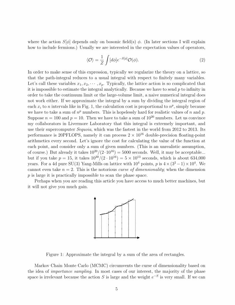
In order to make sense of this expression, typically we regularize the theory on a lattice, sothat the path-integral reduces to a usual integral with respect to finitely many variables.Let’s call these variables x1, x2, · · · , xp. Typically, the lattice action is so complicated thatit is impossible to estimate the integral analytically. Because we have to send p to infinity inorder to take the continuum limit or the large-volume limit, a naive numerical integral doesnot work either. If we approximate the integral by a sum by dividing the integral region ofeach xi to n intervals like in Fig. 1, the calculation cost is proportional to np, simply becausewe have to take a sum of np numbers. This is hopelessly hard for realistic values of n and p.Suppose n = 100 and p = 10. Then we have to take a sum of 1020 numbers. Let us convincemy collaborators in Livermore Laboratory that this integral is extremely important, anduse their supercomputer Sequoia, which was the fastest in the world from 2012 to 2013. Itsperformance is 20PFLOPS, namely it can process 2 × 10¹⁶ double-precision floating-pointarithmetics every second. Let’s ignore the cost for calculating the value of the function ateach point, and consider only a sum of given numbers. (This is an unrealistic assumption,of course.) But already it takes 1020/(2 ·1016) = 5000 seconds. Well, it may be acceptable...but if you take p = 15, it takes 1030/(2 · 1016) = 5 × 10¹³ seconds, which is about 634,000years. For a 4d pure SU(3) Yang-Mills on lattice with 104 points, p is 4× (32−1)×104. Wecannot even take n = 2. This is the notorious curse of dimensionality; when the dimensionp is large it is practically impossible to scan the phase space.
Perhaps when you are reading this article you have access to much better machines, butit will not give you much gain.
Figure 1: Approximate the integral by a sum of the area of rectangles.
Markov Chain Monte Carlo (MCMC) circumvents the curse of dimensionality based onthe idea of importance sampling. In most cases of our interest, the majority of the phasespace is irrelevant because the action S is large and the weight e−S is very small. If we can
5

find important regions in the phase space and invest our resources there, we can avoid thecurse of dimensionality. MCMC enables us to actually do it.
We assume S[x1, x2, · · · , xp] is real and the partition function Z =∫dx1 · · · dxpe−S[x1,x2,··· ,xp]
is finite. In MCMC simulations, we construct a chain of sets of variables x(0) → x(1) →x(2) → · · · x(k) → x(k+1) → · · · satisfying the following conditions:
• Markov Chain. The probability of obtaining x(k+1) from x(k) does not dependon the previous configurations x(0), x(1), · · · , x(k−1). We denote this transitionprobability by T [x(k) → x(k+1)].
• Irreducibility. Any two configurations are connected by finite steps.
• Aperiodicity. The period of a configuration x is given by the greatest commondivisor of possible numbers of steps to come back to itself. When the period is 1 forall configurations, the Markov chain is called aperiodic.
• Detailed balance condition. The transition probability T satisfies e−S[x]T [x →x′] = e−S[x′]T [x′ → x].
Then, the probability distribution of x(k)(k = 1, 2, · · · ) converges to P (x1, x2, · · · , xp) =e−S(x1,x2,··· ,xp)/Z as the chain becomes longer. The expectation values are obtained by takingthe average over the configurations,
〈O〉 =
∫dx1 · · · dxpO(x1, · · · , xp)P (x1, x2, · · · , xp) = lim
n→∞
1
n
n∑k=1
O(x(k)1 , · · · , x(k)
p ). (3)
Note that this is not an approximation; this is exact. Practically we can have only finitelymany configurations, so we can only approximate the right hand side by a finite sum.However there is a systematic way to improve it to arbitrary precision: just make the chainlonger.
Although a proof is rather involved, the importance of each condition can easily beunderstood. Probably the most nontrivial condition for most readers is the detailed balance.Suppose the chain converged to a certain distribution P [x]. Then it has to be ‘stationary’,or equivalently, it should be invariant when shifted one step:∑
x
P [x]T [x → x′] = P [x′] (4)
If P [x] ∝ e−S[x], it follows from the detailed balance condition as∑x
P [x]T [x → x′] =∑x
P [x′]T [x′ → x]
= P [x′]∑x
T [x′ → x]
6
= P [x′]. (5)
I recommend you to follow a complete proof once by looking at an appropriate textbook,but you don’t have to keep it in your brain. You will need it only when you try to inventsomething better than MCMC.
Note that, even if you use exactly the same simulation code, if you take different initialcondition or use different sequence of random numbers, you get different chain. Still, thechain always converges to the same statistical distribution.
2.1 Off-topic: Bayesian analysis
MCMC is powerful outside physics as well. To see a little bit of flavor, let us considerthe Bayes’s theorem,
P (Bi|A) =P (A|Bi)P (Bi)∑j P (A|Bj)P (Bj)
. (6)
Here P (A|B) is the conditional probability: Probability that A is true when the conditionB is satisfied. For example B1, B2, B3 · · · are physicists, high tech engineers, MLB playersetc, and A is millionaires.
Suppose P (A|Bi) and P (Bi) are given (e. g. P (A|B1) = 10−4, P (A|B2) = 0.05, P (A|B3) =0.8, · · · ), and we want to derive P (Bi|A). We can identify Bj and P (A|Bj)P (Bj) with thevalue of the field φ, the path integral weight e−S[φ][dφ]. The denominator
∑j P (A|Bj)P (Bj) =
P (A) is regarded as the partition function Z. Then we can use MCMC to obtain P (Bi|A) ∼e−S[φ][dφ]
Zvia the Bayes’s theorem; namely we can collect many samples and see the distri-
bution.Also if we know f(Bi) ≡ P (C|Bi) you can calculate P (C|A) as
P (C|A) = 〈f〉. (7)
For example C is nice muscle and P (C|B1) = P (C|B2) = 0.01, P (C|B3) = 0.99, · · · .
3 Integration of one-variable functions with Metropo-
lis algorithm
Let us start with the integration of a one-variable function with the Metropolis al-gorithm [12]. In particular, we will consider the simplest example we can imagine: theGaussian integral, S(x) = x2/2. This very basic example contains essentially all importantingredients; all other cases are, ultimately, just technical improvements of this example.
Of course we can handle the Gaussian integral analytically. Also there is a much betteralgorithm for generating Gaussian random numbers (see Appendix B). We use it just foran educational purpose.
7

3.1 Metropolis Algorithm
Let us consider the weight e−S(x), where S(x) is a continuous function of x ∈ R boundedfrom below. We further assume that
∫e−S(x)dx is finite. The Metropolis algorithm gives
us a chain of configurations (or just ‘values’ in the case of single variable) x(0) → x(1) →x(2) → · · · which satisfies the conditions listed above:
1. Randomly choose ∆x ∈ R, and shift x(k) as x(k) → x′ ≡ x(k)+∆x. (∆x and −∆x mustappear with the same probability, so that the detailed balance condition is satisfied.Here we use the uniform random number between ±c, where c > 0 is the ‘step size’.)
2. Metropolis test: Generate a uniform random number r between 0 and 1. If r < e−∆S,where ∆S = S(x′) − S(x(k)), then x(k+1) = x′, i.e. the new value is ‘accepted.’Otherwise x(k+1) = x(k), i.e. the new value is ‘rejected.’
3. Repeat the same for k + 1, k + 2, · · · .
It is an easy exercise to see that all conditions explained above are satisfied:
• It is a Markov Chain, because the past history is not referred either for the selectionof ∆x or the Metropolis test.
• It is irreducible; for example, any x and x′, by taking n large we can make x−x′n
to
be in [−c, c], and there is a nonzero probability that ∆x = x−x′n
appears n times in arow and passes the Metropolis test every time.
• For any x, there is a nonzero probability of ∆x = 0. Hence the period is one for anyx.
• If |x− x′| > c, T [x→ x′] = T [x′ → x] = 0. When |x− x′| ≤ c, both ∆x = x′ − x and∆x′ = x − x′ are chosen with probability 1
2c. Let us assume ∆S = S[x′] − S[x] > 0,
without a loss of generality. Then the change x→ x′ passes the Metropolis test withprobability e−∆S, while x′ → x is always accepted. Hence T [x → x′] = e−∆S
2cand
T [x′ → x] = 12c
, and e−S[x]T [x→ x′] = e−S[x′]T [x′ → x] = e−S[x′]
2c.
3.1.1 How it works
Let me show a sample code written in C:
#include <stdio.h>
#include <stdlib.h>
#include <math.h>
#include <time.h>
8

int main(void)
int iter,niter=100;
int naccept;
double step_size=0.5e0;
double x,backup_x,dx;
double action_init, action_fin;
double metropolis;
srand((unsigned)time(NULL));
/*********************************/
/* Set the initial configuration */
/*********************************/
x=0e0;
naccept=0;
/*************/
/* Main loop */
/*************/
for(iter=1;iter<niter+1;iter++)
backup_x=x;
action_init=0.5e0*x*x;
dx = (double)rand()/RAND_MAX;
dx=(dx-0.5e0)*step_size*2e0;
x=x+dx;
action_fin=0.5e0*x*x;
/*******************/
/* Metropolis test */
/*******************/
metropolis = (double)rand()/RAND_MAX;
if(exp(action_init-action_fin) > metropolis)
/* accept */
naccept=naccept+1;
else
/* reject */
x=backup_x;
/***************/
/* data output */
/***************/
printf("%f\n",x);
9
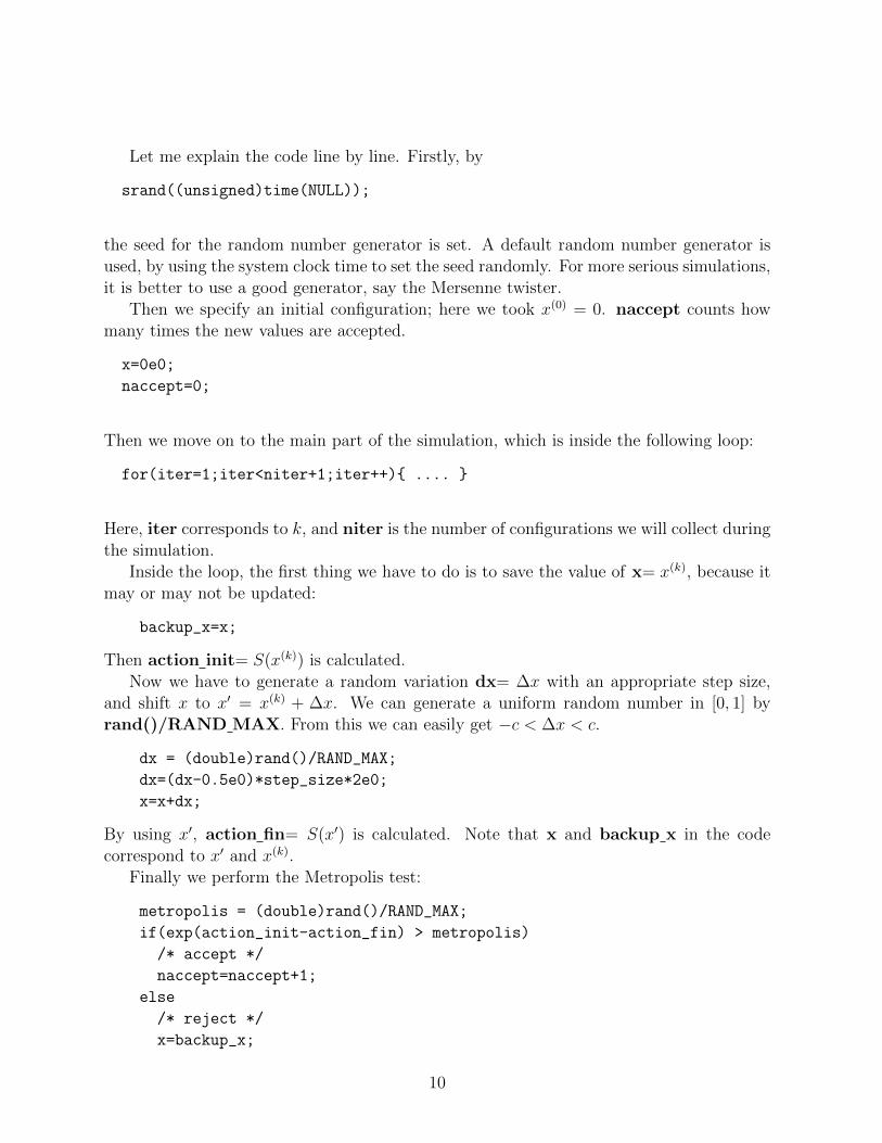
Let me explain the code line by line. Firstly, by
srand((unsigned)time(NULL));
the seed for the random number generator is set. A default random number generator isused, by using the system clock time to set the seed randomly. For more serious simulations,it is better to use a good generator, say the Mersenne twister.
Then we specify an initial configuration; here we took x(0) = 0. naccept counts howmany times the new values are accepted.
x=0e0;
naccept=0;
Then we move on to the main part of the simulation, which is inside the following loop:
for(iter=1;iter<niter+1;iter++) ....
Here, iter corresponds to k, and niter is the number of configurations we will collect duringthe simulation.
Inside the loop, the first thing we have to do is to save the value of x= x(k), because itmay or may not be updated:
backup_x=x;
Then action init= S(x(k)) is calculated.Now we have to generate a random variation dx= ∆x with an appropriate step size,
and shift x to x′ = x(k) + ∆x. We can generate a uniform random number in [0, 1] byrand()/RAND MAX. From this we can easily get −c < ∆x < c.
dx = (double)rand()/RAND_MAX;
dx=(dx-0.5e0)*step_size*2e0;
x=x+dx;
By using x′, action fin= S(x′) is calculated. Note that x and backup x in the codecorrespond to x′ and x(k).
Finally we perform the Metropolis test:
metropolis = (double)rand()/RAND_MAX;
if(exp(action_init-action_fin) > metropolis)
/* accept */
naccept=naccept+1;
else
/* reject */
x=backup_x;
10

metropolis is a uniform random number in [0, 1], which corresponds to r. Depending onthe result of the test, we accept or reject x′.
We emphasize again that all MCMC simulations have exactly the same structure; thereare many fancy algorithms, but essentially, they are all about improving the step x →x+ ∆x.
We take x(0) = 0, and ∆x to be a uniform random number between −0.5 and 0.5. (Aswe will see later, this parameter choice is not optimal.) In Fig. 2, we show the distributionof x(1), x(2), · · · , x(n), for n = 103, 105 and 107. We can see that the distribution convergesto e−x
2/2/√
2π. The expectation values 〈x〉 = 1n
∑nk=1 x
(k) and 〈x2〉 = 1n
∑nk=1
(x(k))2
areplotted in Fig. 3. As n becomes large, they converge to the right values, 0 and 1.
Note that the step size c should be chosen so that the acceptance rate is not too high,not too low. If c is too large, the acceptance rate becomes extremely low, then the value israrely updated. If c is too small, the acceptance rate is almost 1, but the change of the valueat each step is extremely small. In both cases, huge amount of configurations are neededin order to approximate the integration measure accurately. The readers can confirm it bychanging the step size in the sample code. (We will demonstrate it in Sec. 3.2.)
Typically the acceptance rate 30% – 80% is good. But it can heavily depend on thedetail of the system and algorithm; See Sec. 3.2.2 and Sec. 4.2.3 for details.
0
0.1
0.2
0.3
0.4
0.5
0.6
-3 -2 -1 0 1 2 3
0
0.1
0.2
0.3
0.4
0.5
0.6
-3 -2 -1 0 1 2 3
0
0.1
0.2
0.3
0.4
0.5
0.6
-3 -2 -1 0 1 2 3
Figure 2: The distribution of x(1), x(2), · · · , x(n), for n = 103, 105 and 107, and e−x2/2
√2π
.
-0.4
-0.2
0
0.2
0.4
0.6
0.8
1
1.2
1 10 100 1000 10000 100000 1x10⁶
1x10⁷
n
<x2>
<x>
Figure 3: 〈x〉 = 1n
∑nk=1 x
(k) and 〈x2〉 = 1n
∑nk=1
(x(k))2
. As n becomes large, they convergeto the right values, 0 and 1.
11

A bad example
It is instructive to see wrong examples. Let us take ∆x from[−1
2, 1], so that the
detailed balance condition is violated; for example 0 → 1 has a finite probability while1 → 0 is impossible. Then, as we can see from Fig 4, the chain does not converge to theright probability distribution.
0
0.1
0.2
0.3
0.4
0.5
-6 -4 -2 0 2 4 6
Figure 4: The distribution of x(1), x(2), · · · , x(n) for n = 107, with wrong algorithm with
∆x ∈[−1
2, 1]. The dotted line is the right Gaussian distribution e−x
2/2√
2π.
3.2 Autocorrelation and Thermalization
In MCMC, x(k+1) is obtained from x(k). In general, they are correlated. This correlationis called autocorrelation. The autocorrelation can exist over many steps. The autocorre-lation length depends on the detail of the theory, algorithm and the parameter choice.Because of the autocorrelation, some cares are needed.
In the above, we have set x(0) = 0, because we knew it is ‘the most important configura-tion’. What happens if we start with an atypical value, say x(0) = 100? It takes some timefor typical values to appear, due to the autocorrelation. The history of the Monte Carlosimulation with this initial condition is shown in Fig. 5. The value of x eventually reachesto ‘typical values’ |x| . 1 — we often say ‘the configurations are thermalized’ (note thatthe same term ‘thermalized’ has another meaning as well, as we will see shortly) —, but alot of steps are needed. If we include ‘unthermalized’ configurations when we estimate theexpectation values, we will suffer from huge error unless the number of configurations areextremely large. We should discard unthermalized configurations, say n . 1000.3
In generic, more complicated situation, we don’t a priori know what the typical config-urations look like. Still, whether the configurations are thermalized or not can be seen bylooking at several observables. As long as they are changing monotonically, it is plausiblethat the configuration is moving toward a typical one. When they start to oscillate around
3 Number of steps needed for the thermalization is sometimes called ‘burn-in time’ or ‘mixing time’.
12
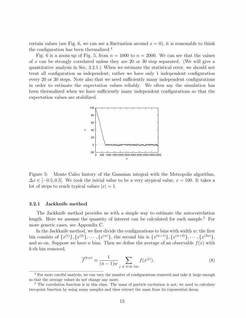
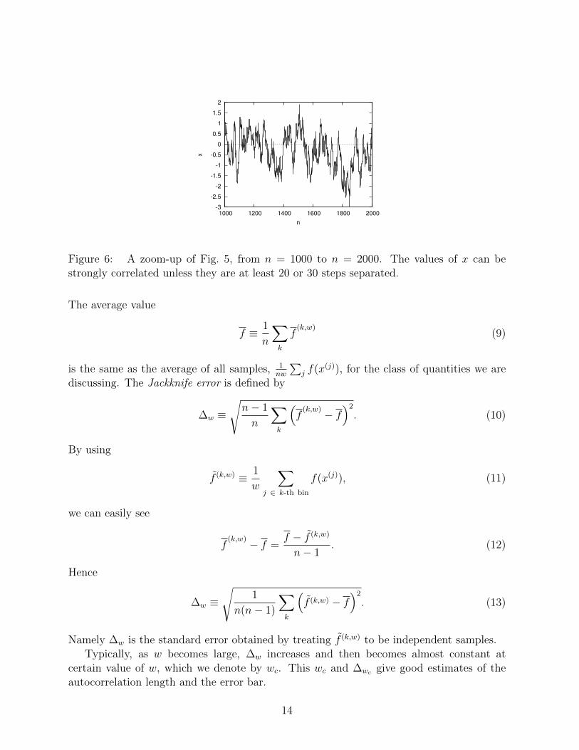
certain values (see Fig. 6, we can see a fluctuation around x = 0), it is reasonable to thinkthe configuration has been thermalized.4
Fig. 6 is a zoom-up of Fig. 5, from n = 1000 to n = 2000. We can see that the valuesof x can be strongly correlated unless they are 20 or 30 step separated. (We will give aquantitative analysis in Sec. 3.2.1.) When we estimate the statistical error, we should nottreat all configuration as independent; rather we have only 1 independent configurationevery 20 or 30 steps. Note also that we need sufficiently many independent configurationsin order to estimate the expectation values reliably. We often say the simulation hasbeen thermalized when we have sufficiently many independent configurations so that theexpectation values are stabilized.
-20
0
20
40
60
80
100
0 500 1000 1500 2000 2500 3000 3500 4000 4500 5000
x
n
Figure 5: Monte Calro history of the Gaussian integral with the Metropolis algorithm,∆x ∈ [−0.5, 0.5]. We took the initial value to be a very atypical value, x = 100. It takes alot of steps to reach typical values |x| ∼ 1.
3.2.1 Jackknife method
The Jackknife method provides us with a simple way to estimate the autocorrelationlength. Here we assume the quantity of interest can be calculated for each sample.5 Formore generic cases, see Appendix C.
In the Jackknife method, we first divide the configurations to bins with width w; the firstbin consists of x(1), x(2), · · · , x(w), the second bin is x(w+1), x(w+2), · · · , x(2w),and so on. Suppose we have n bins. Then we define the average of an observable f(x) withk-th bin removed,
f(k,w) ≡ 1
(n− 1)w
∑j /∈ k-th bin
f(x(j)). (8)
4 For more careful analysis, we can vary the number of configurations removed and take it large enoughso that the average values do not change any more.
5 The correlation function is in this class. The mass of particle excitation is not; we need to calculatetwo-point function by using many samples and then extract the mass from its exponential decay.
13
-3
-2.5
-2
-1.5
-1
-0.5
0
0.5
1
1.5
2
1000 1200 1400 1600 1800 2000
x
n
Figure 6: A zoom-up of Fig. 5, from n = 1000 to n = 2000. The values of x can bestrongly correlated unless they are at least 20 or 30 steps separated.
The average value
f ≡ 1
n
∑k
f(k,w)
(9)
is the same as the average of all samples, 1nw
∑j f(x(j)), for the class of quantities we are
discussing. The Jackknife error is defined by
∆w ≡√n− 1
n
∑k
(f
(k,w) − f)2
. (10)
By using
f (k,w) ≡ 1
w
∑j ∈ k-th bin
f(x(j)), (11)
we can easily see
f(k,w) − f =
f − f (k,w)
n− 1. (12)
Hence
∆w ≡√
1
n(n− 1)
∑k
(f (k,w) − f
)2
. (13)
Namely ∆w is the standard error obtained by treating f (k,w) to be independent samples.Typically, as w becomes large, ∆w increases and then becomes almost constant at
certain value of w, which we denote by wc. This wc and ∆wc give good estimates of theautocorrelation length and the error bar.
14

It can be understood as follows. Let us consider two bin sizes w and 2w. Then
f (k,2w) =f (2k−1,w) + f (2k,w)
2, (14)
∆2w =
√√√√ 1n2
(n2− 1) n/2∑k=1
(f (k,2w) − f
)2
=
√√√√√ 4
n(n− 2)
n/2∑k=1
(f (2k−1,w) − f
)2
+
(f (2k,w) − f
)2
2
. (15)
If w is sufficiently large, f (2k−1,w)− f and f (2k,w)− f should be independent, and the cross-
term(f (2k−1,w) − f
)·(f (2k,w) − f
)should average to zero after summing up with respect
to sufficiently many k. Then
∆2w ∼
√√√√ 1
n2
n∑k=1
(f (k,w) − f
)2
∼ ∆w. (16)
In this way, ∆w becomes approximately constant when w is large enough so that f (k,w) canbe treated as independent samples. (Note that n must also be large for the above estimateto hold.) ∆w is the standard error of these ‘independent samples’.
In Fig. 7, 〈x2〉 and Jackknife error ∆w are shown by using first 50000 samples. We can seethat wc = 50 is a reasonably safe choice; wc = 20 is already in the right ballpark. In Fig. 8,bin-averaged values with w = 50 are plotted. They do look independent. We obtained〈x2〉 = 0.982± 0.012, which agree reasonably well with the analytic answer, 〈x2〉 = 1.
0.965
0.97
0.975
0.98
0.985
0.99
0.995
1
0 20 40 60 80 100
<x
2>
w
Figure 7: 〈x2〉 and Jackknife error ∆w with 50000 samples.
15

-2
-1.5
-1
-0.5
0
0.5
1
1.5
2
2.5
1000 1500 2000 2500 3000 3500 4000 4500 5000
x
n
bin average, w=50
Figure 8: Bin-averaged version of Fig. 6, with bigger window for n, with w = 50.
step size c acceptance c × acceptance
0.5 0.9077 0.454
1.0 0.8098 0.810
2.0 0.6281 1.256
3.0 0.4864 1.459
4.0 0.3911 1.564
6.0 0.2643 1.586
8.0 0.1993 1.594
Table 1: Step size vs acceptance rate, total 10000 samples.
3.2.2 Tuning the simulation parameters
In order to run the simulation efficiently, we should tune parameters so that we canobtain more independent samples with less cost.6
In the current example (Gaussian integral with uniform random number), when the stepsize c is too large, unless ∆x . 1 the configuration is rarely updated; the acceptance rate andthe autocorrelation length scale as 1/c and c, respectively. On the other hand, when c is toosmall, the configurations are almost always updated, but only tiny amount. This is just arandom walk with a step size c, and hence the average change after n steps is c
√n. Therefore
the autocorrelation length should scale as n ∼ 1/c2. We expect the autocorrelation isminimized between these two regions. In Table 1, we have listed the acceptance rate forseveral values of c. We can see that the large-c scaling (c× acceptance ∼ const) sets in ataround c = 2 ∼ c = 4. In Fig. 9 we have shown how 〈x2〉 converges to 1 as the number ofconfigurations increases. We can actually see that c = 2 and c = 4 show faster convergencecompared to too small or too large c.
6 In parallelized simulations, the notion of the cost is more nontrivial because time is money. Sometimesyou may want to invest more electricity and machine resources to obtain the same result with shorter time.
16

0.7
0.75
0.8
0.85
0.9
0.95
1
1.05
1.1
0 20000 40000 60000 80000 100000
<x
2>
n
c=0.5
c=2.0
c=4.0
0.9
0.95
1
1.05
1.1
0 100000 200000 300000 400000 500000
<x
2>
n
c=4.0
c=8.0
c=16.0
Figure 9: 〈x2〉 = 1n
∑nk=1
(x(k))2
for several different step sizes c.
3.3 How to calculate partition function
In MCMC, we cannot directly calculate the partition function Z; we can only see theexpectation values. Usually the partition function is merely a normalization factor of thepath integral measure which does not affect the path integral, so we do not care. Butsometimes it has interesting physical meanings; for example it can be used to test theconjectured dualities between supersymmetric theories.
Suppose you want to calculate Z =∫dxe−S(x), where S(x) is much more complicated
than S0(x) = x2/2. By using MCMC, we can calculate the ratio between Z and Z0 =∫dxe−S0(x) =
√2π,
Z
Z0
=1
Z0
∫dxe−S0 · eS0−S =
⟨eS0−S
⟩0, (17)
where 〈 · 〉0 stands for the expectation value with respect to the action S0. Because weknow Z0 analytically, we can determine Z.
3.3.1 Overlapping problem and its cure
The method described above can always work in principle. In practice, however, itfails when the probability distributions ρ(x) = e−S(x)
Zand ρ0(x) = e−S0(x)
Z0do not have
sufficiently large overlap. As a simple example, let us consider S = (x− c)2/2 (though youcan analytically handle it!). Then ρ(x) and ρ0(x) have peaks around x = c and x = 0,respectively. When c is very large, say c = 100, the value of eS0−S appearing in thesimulation is almost always an extremely small number ∼ e−5000, and once every e+5000
steps or so we get an extremely large number ∼ e+5000. And they average to ZZ0
= 1.Clearly, we cannot get an accurate number if we truncate the sum at a realistic numberof configurations. It happens because of the absence of the overlap of ρ(x) and ρ0(x),or equivalently, because important configurations in two different theories are different;
17

hence the ‘operator’ eS0−S behaves badly at the tail of ρ0(x). This is so-called overlappingproblem.7
In the current situation, the overlapping problem can easily be solved as follows. Letus introduce a series of actions S0, S1, S2, ..., Sk = S. We choose them so that Si and Si+1
are sufficiently close and the ratio Zi+1
Zi, where Zi =
∫dxe−Si(x), can be calculated without
the overlapping problem. For example we can take Si = 12
(x− i
kc)2
with ck∼ 1. Then we
can obtain Z = Zk by calculating Z1
Z0, Z2
Z1, · · · , Zk
Zk−1. The same method can be applied to
any complicated S(x), as long as e−S(x) is real and positive.This rather primitive method is actually powerful; for example the partition function of
ABJM theory [13] at finite coupling and finite N has been calculated accurately by usingthis method [4].
3.4 Common mistakes
Let us see some common mistakes below.
3.4.1 Don’t change step size during the run
Imagine the probability distribution you want to study has a bottleneck like in Fig. 10.
For example if S(x) = − log(e−
x2
2 + e−(x−100)2
2
)then e−S(x) is strongly suppressed between
two peaks at x = 0 and x = 100. By using a small step size c ∼ 1 you can sample oneof the peaks efficiently, but then the other peak cannot be sampled. Then in order to goacross the bottleneck you would be tempted to change the step size c when you come closeto the bottleneck. You would want to make the step size larger so that you can jump overthe bottle neck, or you would want to make the step size smaller so that you can slowlypenetrate into the bottle neck. But if you do so, you obtain a wrong result, because thetransition probability can depend on the past history. You must not change the step sizeduring the simulation.
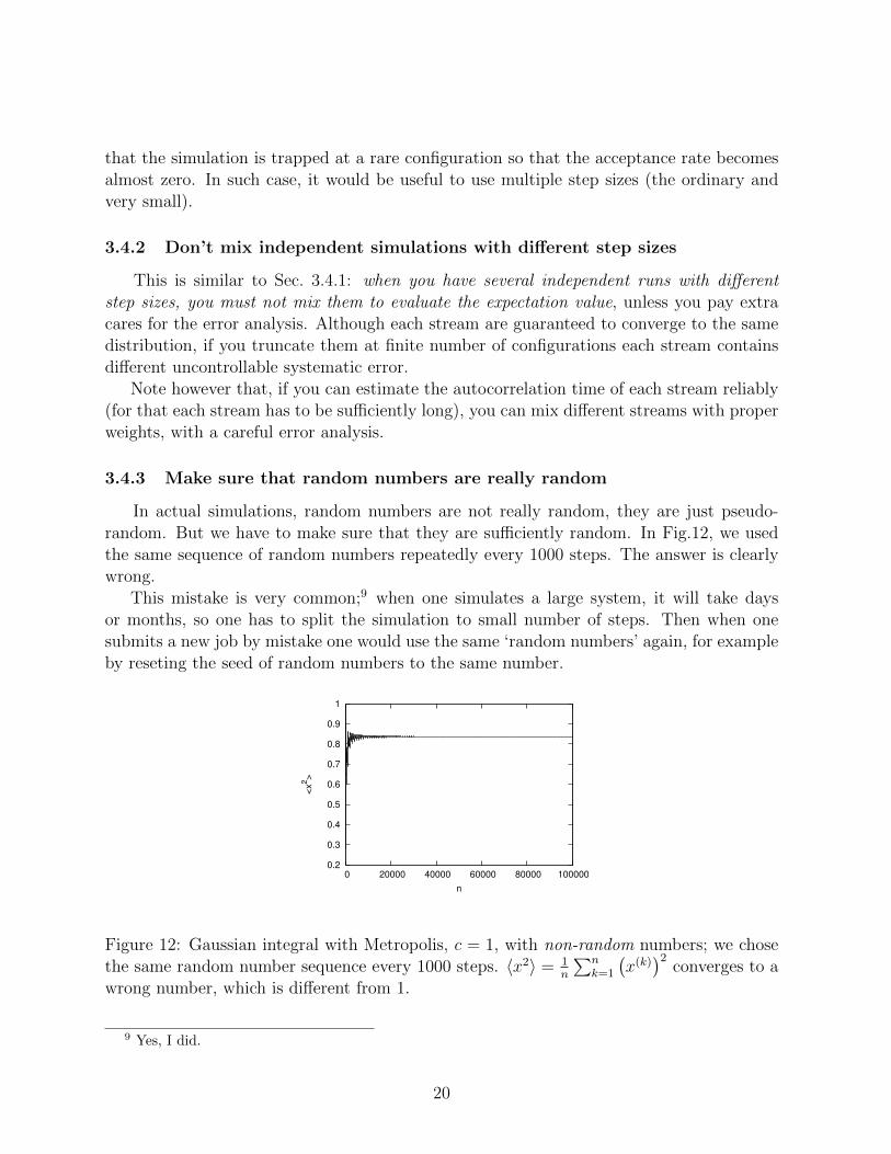
But it does not mean that you cannot use multiple fixed step sizes; it is allowed tochange the step size if the conditions listed in Sec. 2 are not violated. For example we cantake c = 1 for odd steps and c = 100 for even steps; see Fig. 11.
Or we can throw a dice, namely randomly choose step size c = 1, 2, 3, 4, 5, 6 with proba-bility 1/6. As long as the conditions listed in Sec. 2, in particular the detailed balance, arenot violated, you can do whatever you want.
Similar temptation of evil is common in muilti-variable case. For example in the latticegauge theory simulation it often happens that the acceptance is extremely low until thesystem thermalizes. Then we can use smaller step size just to make the system thermalize,and then start actual data-taking with a larger step size.8 Or it occasionally happens
7 In SYM, the overlapping problem can appear combined with the sign problem; we will revisit thispoint in Sec. 7.2.
8 Another common strategy to reach the thermalization is to turn off the Metropolis test.
18
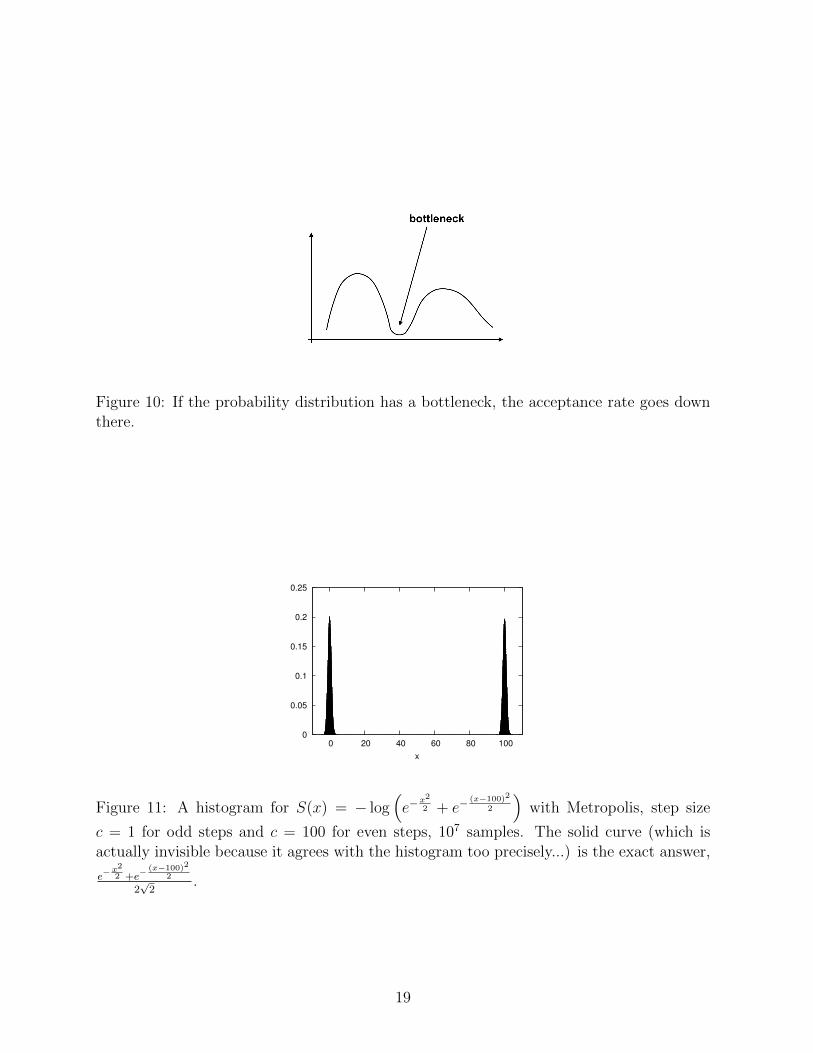
Figure 10: If the probability distribution has a bottleneck, the acceptance rate goes downthere.
0
0.05
0.1
0.15
0.2
0.25
0 20 40 60 80 100
x
Figure 11: A histogram for S(x) = − log(e−
x2
2 + e−(x−100)2
2
)with Metropolis, step size
c = 1 for odd steps and c = 100 for even steps, 107 samples. The solid curve (which isactually invisible because it agrees with the histogram too precisely...) is the exact answer,
e−x2
2 +e−(x−100)2
2
2√
2.
19
that the simulation is trapped at a rare configuration so that the acceptance rate becomesalmost zero. In such case, it would be useful to use multiple step sizes (the ordinary andvery small).
3.4.2 Don’t mix independent simulations with different step sizes
This is similar to Sec. 3.4.1: when you have several independent runs with differentstep sizes, you must not mix them to evaluate the expectation value, unless you pay extracares for the error analysis. Although each stream are guaranteed to converge to the samedistribution, if you truncate them at finite number of configurations each stream containsdifferent uncontrollable systematic error.
Note however that, if you can estimate the autocorrelation time of each stream reliably(for that each stream has to be sufficiently long), you can mix different streams with properweights, with a careful error analysis.
3.4.3 Make sure that random numbers are really random
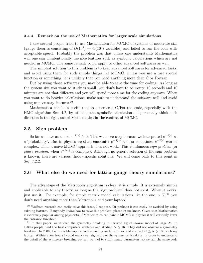
In actual simulations, random numbers are not really random, they are just pseudo-random. But we have to make sure that they are sufficiently random. In Fig.12, we usedthe same sequence of random numbers repeatedly every 1000 steps. The answer is clearlywrong.
This mistake is very common;9 when one simulates a large system, it will take daysor months, so one has to split the simulation to small number of steps. Then when onesubmits a new job by mistake one would use the same ‘random numbers’ again, for exampleby reseting the seed of random numbers to the same number.
0.2
0.3
0.4
0.5
0.6
0.7
0.8
0.9
1
0 20000 40000 60000 80000 100000
<x
2>
n
Figure 12: Gaussian integral with Metropolis, c = 1, with non-random numbers; we chosethe same random number sequence every 1000 steps. 〈x2〉 = 1
n
∑nk=1
(x(k))2
converges to awrong number, which is different from 1.
9 Yes, I did.
20
3.4.4 Remark on the use of Mathematica for larger scale simulations
I saw several people tried to use Mathematica for MCMC of systems of moderate size(gauge theories consisting of O(103) — O(104) variables) and failed to run the code withacceptable speed. Probably the problem was that unless one understands Mathematicawell one can unintentionally use nice features such as symbolic calculations which are notneeded in MCMC. The same remark could apply to other advanced softwares as well.
The simplest solution to this problem is to keep advanced softwares for advanced tasks,and avoid using them for such simple things like MCMC. Unless you use a rare specialfunction or something, it is unlikely that you need anything more than C or Fortran.
But by using those softwares you may be able to save the time for coding. As long asthe system size you want to study is small, you don’t have to to worry; 10 seconds and 10minutes are not that different and you will spend more time for the coding anyways. Whenyou want to do heavier calculations, make sure to understand the software well and avoidusing unnecessary features.10
Mathematica can be a useful tool to generate a C/Fortran code, especially with theHMC algorithm Sec. 4.2, by utilizing the symbolic calculations. I personally think suchdirection is the right use of Mathematica in the context of MCMC.
3.5 Sign problem
So far we have assumed e−S(x) ≥ 0. This was necessary because we interpreted e−S(x) asa ‘probability’. But in physics we often encounter e−S(x) < 0, or sometimes e−S(x) can becomplex. Then a naive MCMC approach does not work. This is infamous sign problem (orphase problem, when e−S(x) is complex). Although no generic solution of the sign problemis known, there are various theory-specific solutions. We will come back to this point inSec. 7.2.2.
3.6 What else do we need for lattice gauge theory simulations?
The advantage of the Metropolis algorithm is clear: it is simple. It is extremely simpleand applicable to any theory, as long as the ‘sign problem’ does not exist. When it works,just use it. For example, for simple matrix model calculations like the one in [2],11 youdon’t need anything more than Metropolis and your laptop.
10 Wolfram research can easily solve this issue, I suppose. Or perhaps it can easily be avoided by usingexisting features. If anybody knows how to solve this problem, please let me know. Given that Mathematicais extremely popular among physicists, if Mathematica can handle MCMC in physics it will certainly lowerthe entrance threshold.
11 In that paper, we studied the symmetry breaking in Twisted Eguchi-Kawai model at large N . In1980’s people used the best computers available and studied N . 16. They did not observe a symmetrybreaking. In 2006, I wrote a Metropolis code spending an hour or so, and studied 25 . N . 100 with mylaptop. Within a few hours I could see a clear signature of the symmetry breaking. In order to understandthe detail of the symmetry breaking pattern we had to study many parameters, so we ran the same code
21

But our budget is limited and we cannot live forever. So sometimes we have to reducethe cost and make simulations faster. We should use better algorithms, better lattice actionsand better observables, which are ‘better’ in the following sense:
• The autocorrelation length is shorter.
• Easier to parallelize. In lattice gauge theory, it typically means that we should utilizethe sparseness of the Dirac operator.
• Find good observables and good measurement methods which are easier to calculate,have less statistical fluctuations, and/or show faster convergence to the continuumlimit.
For quantum field theories, especially when the fermions are involved, HMC is effective.RHMC is a variant of HMC which is applicable to SYM.
4 Integration of multiple variables and bosonic QFT
Once a regularization is given, the path-integral is merely an integral with multiplevariables. Hence let us start with a simple case of a matrix integral, then proceed to QFT.
4.1 Metropolis for multiple variables
Generalization of the Metropolis algorithm (Sec. 3.1) to multiple variables (x1, x2, · · · , xp)is straightforward. For example, we can do as follows:
1. For all i = 1, 2, · · · , p, randomly choose ∆xi ∈ [−ci,+ci], and shift x(k)i as x
(k)i → x′i ≡
x(k)i + ∆xi. Note that the step size ci can be different for different xi.
2. Metropolis test: Generate a uniform random number r between 0 and 1. If r <eS[x(k)]−S[x′], x(k+1) = x′, i.e. the new configuration is ‘accepted.’ Otherwisex(k+1) = x(k), i.e. the new configuration is ‘rejected.’
3. Repeat the same for k + 1, k + 2, · · · .
One can also do as follows:
1. Randomly choose ∆x1 ∈ [−c1,+c1], and shift x(k)1 as x
(k)1 → x′1 ≡ x
(k)1 + ∆x1.
2. Metropolis test: Generate a uniform random number r between 0 and 1. If r <eS[x(k)]−S[x′], x
(k+1)1 = x′1, i.e. the new value is ‘accepted.’ Otherwise x
(k+1)1 = x
(k)1 ,
i.e. the new configuration is ‘rejected.’ For other values of i we don’t do anything,namely x
(k+1)i = x
(k)i for i = 2, 3, · · · , p.
on a cluster machine. One of my collaborators was serious enough to write a more sophisticated code togo to much larger N , with which we could study N & 100. Note that it is a story from 2006 to 2007; nowyou can do much better job with Metropolis and your laptop.
22
3. Repeat the same for i = 2, 3, · · · , p.
4. Repeat the same for k + 1, k + 2, · · · .
4.1.1 How it works
Let us consider a one matrix model,
S[φ] = NTr
(1
2φ2 + V (φ)
), (18)
where φ is an N ×N Hermitian matrix, φji = φ∗ij. The potential V (φ) can be anything aslong as the partition function is convergent; say V (φ) = φ4.
The code has exactly the same structure as the sample code in Sec. 3.1; we shouldcalculate S[φ] instead of the Gaussian weight, and instead of x we can shift φ by using N2
real random numbers.As N gets larger, more and more portion of the integral region becomes unimportant.
Therefore, if we vary all the components simultaneously, ∆S is typically large and theacceptance rate is very small, unless we take the step size to be small. To avoid it, we canvary one component at each time. Note that, when only φij and φji = φ∗ij are varied, oneshould save the computational cost by calculating φij-dependent part instead of S[φ] itself;the latter costs O(N3), though the former costs only O(N2).
4.2 Hybrid Monte Carlo (HMC) Algorithm
The important configurations are like bottom of a valley; the altitude is the value ofthe action. This is a valley in the phase space, whose dimension is very large. So if theconfiguration is literally randomly varied, like in the Metropolis algorithm, the action almostalways increases a lot. Hence with the Metropolis algorithm the acceptance rate is smallunless the step size is extremely small, and it causes rather long autocorrelation length. TheHybrid Monte Carlo (HMC) algorithm [14] avoids the problem of a long autocorrelation byeffectively crawling along the bottom of the valley; this is a ‘hybrid’ of molecular dynamicalmethod and Metropolis algorithm.
In HMC algorithm, sets of configurations x(k) (k = 0, 1, 2, · · · ) are generated in thefollowing manner. Firstly, x(0) can be arbitrary. Once x(k) is obtained, x(k+1) isobtained as follows.
1. Randomly generate auxiliary momenta P(k)i , which are ‘conjugate’ to x
(k)i , with prob-
abilities 1√2πe−(P
(k)i )2/2. To generate Gaussian random numbers, the Box-Muller algo-
rithm is convenient; see Appendix B.
2. Calculate the ‘Hamiltonian’ Hi = S[x(k)] + 12
∑i(P
(k)i )2.
23
3. Then we consider ‘time evolution’ along an auxiliary time τ (which is not the Eu-clidean time!). We set the initial condition to be x(k)(τ = 0) = x(k) and P (k)(τ =0) = P (k), and use the leap frog method (see below) to calculate x(k)(τf ) and P (k)(τf ),where τf is related to the input parameters ∆τ and Nτ by τf = Nτ∆τ .
This process is called ‘molecular evolution.’
4. Calculate Hf = S[x(k)(τf )] + 12
∑i(P
(k)i (τf ))
2.
5. Metropolis test: Generate a uniform random number r between 0 and 1. If r < eHi−Hf ,x(k+1) = x(k)(τf ), i.e. the new configuration is ‘accepted.’ Otherwise x(k+1) = x(k),i.e. the new configuration is ‘rejected.’
At first sight it is a rather complicated algorithm. Why do we introduce such auxiliarydynamical system? The key is the ‘energy conservation’.
Just like Metropolis, the change of the configuration is random due to the randomnessof the choice of auxiliary momenta Pi. If we just compared the initial and final values ofthe action, the change would be equally large. However in HMC the change of the auxiliaryHamiltonian matters in the Metropolis test. (Please accept this fact for the moment, in thenext paragraph we will explain the reason.) If we keep Nτ∆τ fixed and send Nτ to infinity,then the Hamiltonian is exactly conserved and new configurations are always accepted. Bytaking Nτ∆τ to be large, new configurations can be substantially different from the oldones. (Of course, calculation cost increase with Nτ . So we have to find a sweet spot, withmoderately large Nτ and moderately small ∆τ .)
To check the detailed balance condition e−S[x]T [x → x′] = e−S[x′]T [x′ → x],note that the leap-frog method is designed so that the molecular evolution is reversible;namely, if we start with x(k)(τf ) and −P (k)(τf ), the final configuration is x(k)(τ = 0)and −P (k)(τ = 0). Hence, if x, p evolves to x′, p′, then (by assuming H − H ′ < 0without loss of generality) e−S[x]T [x → x′] ∝ e−S[x]e−p
2/2, while e−S[x′]T [x′ → x] ∝e−S[x′]e−p
′2/2e−S[x]−p2/2+S[x′]+p′2/2 = e−S[x]e−p2/2, with the same proportionality factor.
In fact the HMC algorithm works even when we take different τ for each xi; see Sec. 4.3.We can use different τ on depending the field, momentum of the mode, etc. The HMCalgorithm is powerful especially when we have to deal with fermions, as we will explainlater.
4.2.1 Leap frog method
The leap frog method is a clever way to discretize the continuum Hamiltonian equationkeeping the reversibility, which is crucial for assuring the detailed balance condition.
The continuum Hamiltonian equation is given by
dpidτ
= −∂H∂xi
= − ∂S∂xi
,dxidτ
=∂H
∂pi= pi. (19)
24
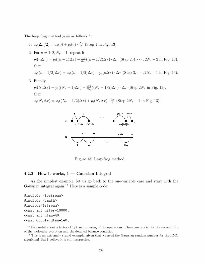
The leap frog method goes as follows12:
1. xi(∆τ/2) = xi(0) + pi(0) · ∆τ2
(Step 1 in Fig. 13).
2. For n = 1, 2, Nτ − 1, repeat it:
pi(n∆τ) = pi((n− 1)∆τ)− ∂S∂xi
((n− 1/2)∆τ) ·∆τ (Step 2, 4, · · · , 2Nτ − 2 in Fig. 13),
then
xi((n+ 1/2)∆τ) = xi((n− 1/2)∆τ) + pi(n∆τ) ·∆τ (Step 3, · · · , 2Nτ − 1 in Fig. 13).
3. Finally,
pi(Nτ∆τ) = pi((Nτ − 1)∆τ)− ∂S∂xi
((Nτ − 1/2)∆τ) ·∆τ (Step 2Nτ in Fig. 13),
then
xi(Nτ∆τ) = xi((Nτ − 1/2)∆τ) + pi(Nτ∆τ) · ∆τ2
(Step 2Nτ + 1 in Fig. 13).
Figure 13: Leap-frog method.
4.2.2 How it works, 1 — Gaussian Integral
As the simplest example, let us go back to the one-variable case and start with theGaussian integral again.13 Here is a sample code:
#include <iostream>
#include <cmath>
#include<fstream>
const int niter=10000;
const int ntau=40;
const double dtau=1e0;
12 Be careful about a factor of 1/2 and ordering of the operations. These are crucial for the reversibilityof the molecular evolution and the detailed balance condition.
13 This is an extremely stupid example, given that we need the Gaussian random number for the HMCalgorithm! But I believe it is still instructive.
25

/******************************************************************/
/*** Gaussian Random Number Generator with Box Muller Algorithm ***/
/******************************************************************/
int BoxMuller(double& p, double& q)
double pi;
double r,s;
pi=2e0*asin(1e0);
//uniform random numbers between 0 and 1
r = (double)rand()/RAND_MAX;
s = (double)rand()/RAND_MAX;
//Gaussian random numbers,
//with weights proportional to e^-p^2/2 and e^-q^2/2
p=sqrt(-2e0*log(r))*sin(2e0*pi*s);
q=sqrt(-2e0*log(r))*cos(2e0*pi*s);
return 0;
/*********************************/
/*** Calculation of the action ***/
/*********************************/
// When you change the action, you should also change dH/dx,
// specified in "calc_delh".
double calc_action(const double x)
double action=0.5e0*x*x;
return action;
/**************************************/
/*** Calculation of the Hamiltonian ***/
/**************************************/
double calc_hamiltonian(const double x,const double p)
double ham;
ham=calc_action(x);
ham=ham+0.5e0*p*p;
return ham;
26

/****************************/
/*** Calculation of dH/Dx ***/
/****************************/
// Derivative of the Hamiltonian with respect to x,
// which is equivalent to the derivative of the action.
// When you change "calc_action", you have to change this part as well.
double calc_delh(const double x)
double delh=x;
return delh;
/***************************/
/*** Molecular evolution ***/
/***************************/
int Molecular_Dynamics(double& x,double& ham_init,double& ham_fin)
double p;
double delh;
double r1,r2;
BoxMuller(r1,r2);
p=r1;
//*** calculate Hamiltonian ***
ham_init=calc_hamiltonian(x,p);
//*** first step of leap frog ***
x=x+p*0.5e0*dtau;
//*** 2nd, ..., Ntau-th steps ***
for(int step=1; step!=ntau; step++)
delh=calc_delh(x);
p=p-delh*dtau;
x=x+p*dtau;
//*** last step of leap frog ***
delh=calc_delh(x);
p=p-delh*dtau;
x=x+p*0.5e0*dtau;
//*** calculate Hamiltonian again ***
ham_fin=calc_hamiltonian(x,p);
return 0;
27
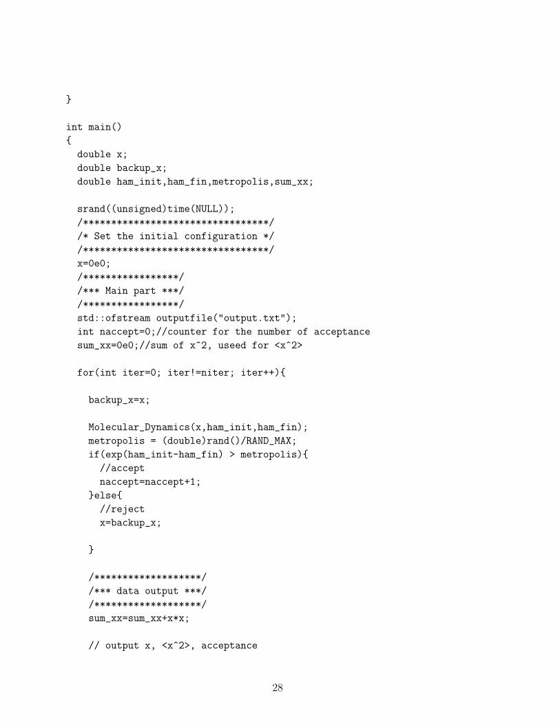
int main()
double x;
double backup_x;
double ham_init,ham_fin,metropolis,sum_xx;
srand((unsigned)time(NULL));
/*********************************/
/* Set the initial configuration */
/*********************************/
x=0e0;
/*****************/
/*** Main part ***/
/*****************/
std::ofstream outputfile("output.txt");
int naccept=0;//counter for the number of acceptance
sum_xx=0e0;//sum of x^2, useed for <x^2>
for(int iter=0; iter!=niter; iter++)
backup_x=x;
Molecular_Dynamics(x,ham_init,ham_fin);
metropolis = (double)rand()/RAND_MAX;
if(exp(ham_init-ham_fin) > metropolis)
//accept
naccept=naccept+1;
else
//reject
x=backup_x;
/*******************/
/*** data output ***/
/*******************/
sum_xx=sum_xx+x*x;
// output x, <x^2>, acceptance
28

std::cout << x << ’ ’ << sum_xx/((double)(iter+1)) << ’ ’ <<
((double)naccept)/((double)iter+1) << std::endl;
outputfile << x << ’ ’ << sum_xx/((double)(iter+1)) << ’ ’ <<
((double)naccept)/((double)iter+1) << std::endl;
outputfile.close();
return 0;
At the beginning of the code, a few parameters are set. niter is the number of sampleswe will collect; ntau is Nτ ; and dtau is ∆τ .
Then several routines/functions are defined:
• BoxMuller generates Gaussian random numbers by using the Box-Muller algorithm.We have to be careful about the normalization of the Gaussian here. It will be a kindof confusing when you go to complex variables; see the case of matrix integral inSec. 4.2.3.
• calc action calculates the action S[x]. In this case it is just S[x] = x2
2. It is called in
calc hamiltonian.
• calc hamiltonian adds p2
2to the action and returns the Hamiltonian. It is called in
Molecular Dynamics.
• calc delh returns dHdx
= dSdx
= x. It is called in Molecular Dynamics.
• Molecular Dynamics performs one molecular evolution and returns the value of xafter the evolution and the values of the Hamiltonian before and after the evolution.
When the action S[x] is changed to more complicated functions, you have to rewritecalc action and calc delh accordingly.
In main, the only difference from Metropolis is that Molecular Dynamics is usedinstead of a naive random change (x→ x+ ∆x with random ∆x), and the Metropolis testis performed by using ∆H instead of ∆S.
4.2.3 How it works, 2 — Matrix Integral
Next let us consider the same example as before,
S[φ] = NTr
(1
2φ2 +
1
4φ4
), (20)
29
where φ is N×N Hermitian, and use the convention explained above. Then the force termsare
dPijdτ
= − ∂S
∂φji= −φij −
(φ3)ij,
dφijdτ
= Pij. (21)
The simulation code is very simple. Here is a one in Fortran 90:14
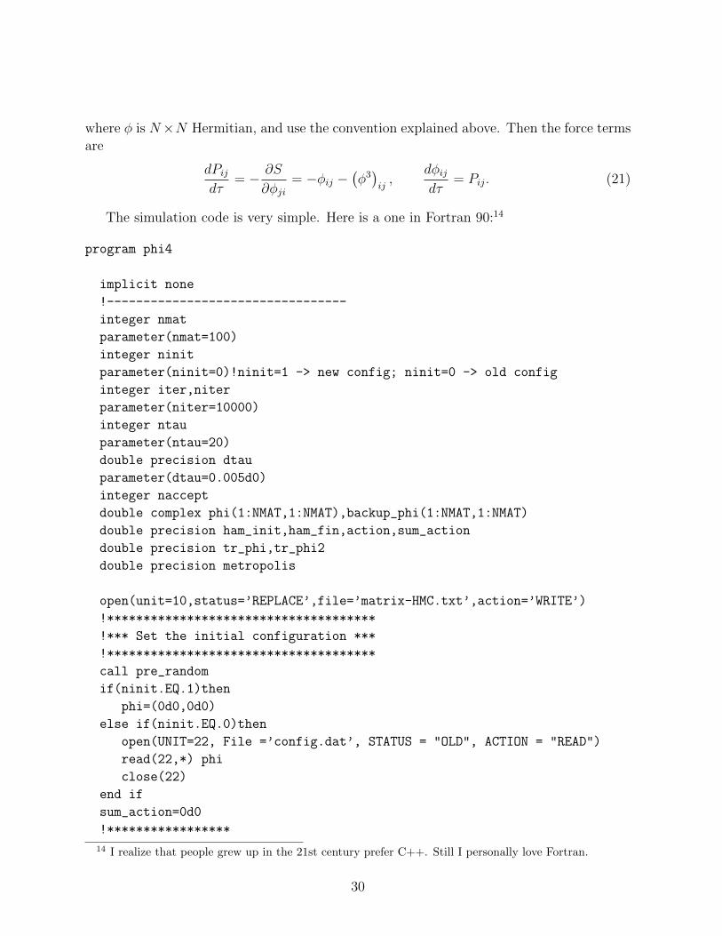
program phi4
implicit none
!---------------------------------
integer nmat
parameter(nmat=100)
integer ninit
parameter(ninit=0)!ninit=1 -> new config; ninit=0 -> old config
integer iter,niter
parameter(niter=10000)
integer ntau
parameter(ntau=20)
double precision dtau
parameter(dtau=0.005d0)
integer naccept
double complex phi(1:NMAT,1:NMAT),backup_phi(1:NMAT,1:NMAT)
double precision ham_init,ham_fin,action,sum_action
double precision tr_phi,tr_phi2
double precision metropolis
open(unit=10,status=’REPLACE’,file=’matrix-HMC.txt’,action=’WRITE’)
!*************************************
!*** Set the initial configuration ***
!*************************************
call pre_random
if(ninit.EQ.1)then
phi=(0d0,0d0)
else if(ninit.EQ.0)then
open(UNIT=22, File =’config.dat’, STATUS = "OLD", ACTION = "READ")
read(22,*) phi
close(22)
end if
sum_action=0d0
!*****************
14 I realize that people grew up in the 21st century prefer C++. Still I personally love Fortran.
30

!*** Main part ***
!*****************
naccept=0 !counter for the number of acceptance
do iter=1,niter
backup_phi=phi
call Molecular_Dynamics(nmat,phi,dtau,ntau,ham_init,ham_fin)
!***********************
!*** Metropolis test ***
!***********************
call random_number(metropolis)
if(dexp(ham_init-ham_fin) > metropolis)then
!accept
naccept=naccept+1
else
!reject
phi=backup_phi
end if
!*******************
!*** data output ***
!*******************
call calc_action(nmat,phi,action)
sum_action=sum_action+action
write(10,*)iter,action/dble(nmat*nmat),sum_action/dble(iter)/dble(nmat*nmat),&
&dble(naccept)/dble(iter)
end do
close(10)
open(UNIT = 22, File = ’config.dat’, STATUS = "REPLACE", ACTION = "WRITE")
write(22,*) phi
close(22)
end program Phi4
Again, it is very similar to a Metropolis code; randomly change the configuration,perform the Metropolis test, randomly change the configuration, perform the Metropolistest,.... In Molecular Dynamics, random momentum is generated with the normalizationexplained below (26), the molecular evolution performed, and Hi and Hf are calculated.Subroutines calc hamiltonian and calc force (which corresponds to calc delh in the pre-
31

vious example) return the Hamiltonian and the force term ∂H∂φji
= ∂S∂φji
; it literally calculatesproducts of matrices. Another subroutine calc action is also simple. Let’s see them oneby one.15
Molecular Dynamics
subroutine Molecular_Dynamics(nmat,phi,dtau,ntau,ham_init,ham_fin)
implicit none
integer nmat
integer ntau
double precision dtau
double precision r1,r2
double precision ham_init,ham_fin
double complex phi(1:NMAT,1:NMAT)
double complex P_phi(1:NMAT,1:NMAT)
double complex delh(1:NMAT,1:NMAT)
integer imat,jmat,step
!*** randomly generate auxiliary momenta ***
do imat=1,nmat-1
do jmat=imat+1,nmat
call BoxMuller(r1,r2)
P_phi(imat,jmat)=dcmplx(r1/dsqrt(2d0))+dcmplx(r2/dsqrt(2d0))*(0D0,1D0)
P_phi(jmat,imat)=dcmplx(r1/dsqrt(2d0))-dcmplx(r2/dsqrt(2d0))*(0D0,1D0)
end do
end do
do imat=1,nmat
call BoxMuller(r1,r2)
P_phi(imat,imat)=dcmplx(r1)
end do
!*** calculate Hamiltonian ***
call calc_hamiltonian(nmat,phi,P_phi,ham_init)
!*** first step of leap frog ***
phi=phi+P_phi*dcmplx(0.5d0*dtau)
!*** 2nd, ..., Ntau-th steps ***
step=1
do while (step.LT.ntau)
15 For routines which are not explained below, please look at the sample code at https://github.com/MCSMC/MCMC_sample_codes.
32

step=step+1
call calc_force(delh,phi,nmat)
P_phi=P_phi-delh*dtau
phi=phi+P_phi*dcmplx(dtau)
end do
!*** last step of leap frog ***
call calc_force(delh,phi,nmat)
P_phi=P_phi-delh*dtau
phi=phi+P_phi*dcmplx(0.5d0*dtau)
!*** calculate Hamiltonian ***
call calc_hamiltonian(nmat,phi,P_phi,ham_fin)
return
END subroutine Molecular_Dynamics
The inputs are the matrix size nmat= N , the matrix phi= φ(k), the step size andnumber of steps for the molecular evolution, dtau= ∆τ and ntau= Nτ . The output isphi= φ′ and ham init= Hi, ham fin= Hf . Note that the auxiliary momentum is neitherinput nor output; it is randomly generated every time in this subroutine.
Firstly random momentum Pφ is generated. BoxMuller(r1,r2) generates random num-
bers r1 and r2 with the Gaussian weight e−r21/2√2π
, e−r22/2√2π
. Note that Pφ is Hermitian, Pφ = P †φ.
Hence we take Pφ,ii to be real, Pφ,ii = r1, and Pφ,ij = P ∗φ,ji = (r1 + ir2)/√
2 for i < j. A
factor 1/√
2 is necessary in order to adjust the normalization.
!*** randomly generate auxiliary momenta ***
do imat=1,nmat-1
do jmat=imat+1,nmat
call BoxMuller(r1,r2)
P_phi(imat,jmat)=dcmplx(r1/dsqrt(2d0))+dcmplx(r2/dsqrt(2d0))*(0D0,1D0)
P_phi(jmat,imat)=dcmplx(r1/dsqrt(2d0))-dcmplx(r2/dsqrt(2d0))*(0D0,1D0)
end do
end do
do imat=1,nmat
call BoxMuller(r1,r2)
P_phi(imat,imat)=dcmplx(r1)
end do
Then we calculate the initial value of the Hamiltonian:
!*** calculate Hamiltonian ***
call calc_hamiltonian(nmat,phi,P_phi,ham_init)
33
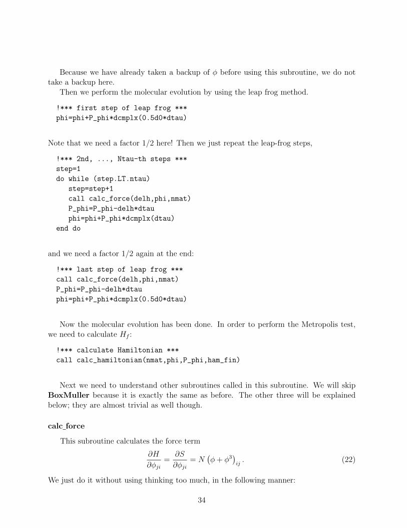
Because we have already taken a backup of φ before using this subroutine, we do nottake a backup here.
Then we perform the molecular evolution by using the leap frog method.
!*** first step of leap frog ***
phi=phi+P_phi*dcmplx(0.5d0*dtau)
Note that we need a factor 1/2 here! Then we just repeat the leap-frog steps,
!*** 2nd, ..., Ntau-th steps ***
step=1
do while (step.LT.ntau)
step=step+1
call calc_force(delh,phi,nmat)
P_phi=P_phi-delh*dtau
phi=phi+P_phi*dcmplx(dtau)
end do
and we need a factor 1/2 again at the end:
!*** last step of leap frog ***
call calc_force(delh,phi,nmat)
P_phi=P_phi-delh*dtau
phi=phi+P_phi*dcmplx(0.5d0*dtau)
Now the molecular evolution has been done. In order to perform the Metropolis test,we need to calculate Hf :
!*** calculate Hamiltonian ***
call calc_hamiltonian(nmat,phi,P_phi,ham_fin)
Next we need to understand other subroutines called in this subroutine. We will skipBoxMuller because it is exactly the same as before. The other three will be explainedbelow; they are almost trivial as well though.
calc force
This subroutine calculates the force term
∂H
∂φji=
∂S
∂φji= N
(φ+ φ3
)ij. (22)
We just do it without using thinking too much, in the following manner:
34

subroutine calc_force(delh,phi,nmat)
implicit none
integer nmat
double complex phi(1:NMAT,1:NMAT),phi2(1:NMAT,1:NMAT),phi3(1:NMAT,1:NMAT)
double complex delh(1:NMAT,1:NMAT)
integer imat,jmat,kmat
!*** phi2=phi*phi, phi3=phi*phi*phi ***
phi2=(0d0,0d0)
phi3=(0d0,0d0)
do imat=1,nmat
do jmat=1,nmat
do kmat=1,nmat
phi2(imat,jmat)=phi2(imat,jmat)+phi(imat,kmat)*phi(kmat,jmat)
end do
end do
end do
do imat=1,nmat
do jmat=1,nmat
do kmat=1,nmat
phi3(imat,jmat)=phi3(imat,jmat)+phi2(imat,kmat)*phi(kmat,jmat)
end do
end do
end do
!*** delh=dH/dphi ***
delh=phi+phi3
delh=delh*dcmplx(nmat)
return
END subroutine Calc_Force
calc hamiltonian
This subroutine just returns H = 12TrP 2+S[φ]. Firstly another subroutine calc action,
which calculates the action, is called. Then 12TrP 2 is added. It is too simple and looks
almost stupid, but most things needed for MCMC codes are like this.
SUBROUTINE calc_hamiltonian(nmat,phi,P_phi,ham)
35

implicit none
integer nmat
double precision action,ham
double complex phi(1:NMAT,1:NMAT)
double complex P_phi(1:NMAT,1:NMAT)
integer imat,jmat
call calc_action(nmat,phi,action)
ham=action
do imat=1,nmat
do jmat=1,nmat
ham=ham+0.5d0*dble(P_phi(imat,jmat)*P_phi(jmat,imat))
end do
end do
return
END SUBROUTINE calc_hamiltonian
calc action
This subroutine just returns S[φ]. We honestly write down everything. It is tedious butstraightforward. You just have to be patient.
SUBROUTINE calc_action(nmat,phi,action)
implicit none
integer nmat
double precision action
double complex phi(1:NMAT,1:NMAT)
double complex phi2(1:NMAT,1:NMAT)
integer imat,jmat,kmat
!*** phi2=phi*phi ***
phi2=(0d0,0d0)
do imat=1,nmat
do jmat=1,nmat
do kmat=1,nmat
phi2(imat,jmat)=phi2(imat,jmat)+phi(imat,kmat)*phi(kmat,jmat)
end do
end do
36

Nτ acceptance acceptance/Nτ
4 0.0633 0.01583
6 0.3418 0.05697
8 0.6023 0.07529
10 0.7393 0.07393
20 0.9333 0.04667
Table 2: Acceptance rate for several choices of Nτ , with Nτ∆τ = 0.1, matrix size N = 100.We started the measurement runs with well thermalized configurations and collected 10000samples for each parameter choice.
end do
action=0d0
!*** Tr phi^2 term ***
do imat=1,nmat
action=action+0.5d0*dble(phi2(imat,imat))
end do
!*** Tr phi^4 term ***
do imat=1,nmat
do jmat=1,nmat
action=action+0.25d0*dble(phi2(imat,jmat)*phi2(jmat,imat))
end do
end do
!*** overall normalization ***
action=action*dble(nmat)
return
END SUBROUTINE calc_action
Simulation
In order to see how we can adjust the simulation parameters, let us vary Nτ and ∆τkeeping the product Nτ∆τ to be 0.1. Then the acceptance rate changes as follows shown inTable 2. Roughly speaking, the simulation cost is proportional to Nτ . When Nτ∆τ is fixed,the matrix φ changes more or less the same amount by the molecular evolution, regardlessof Nτ . Therefore, the rate of change is proportional to the acceptance rate. Hence thechange per cost is (acceptance)/Nτ . We should maximize it. So we should use Nτ = 8 or10. In Fig. 14 we have plotted 〈S/N2〉 = 1
n
∑nk=1 S[φ(k)] for several different values of Nτ
37

by taking the horizontal axis to be ‘cost’= n×Nτ . We can see that Nτ = 8, 10 are actuallycost effective.
Ideally we should do similar cost analysis varying Nτ∆τ , and estimate the autocorrela-tion length as well, to achieve more independent configurations with less cost.
Figure 14: 〈S〉/N2 = 1n
∑nk=1 S[φ(k)] with N = 100, for several different values of Nτ . The
horizontal axis is n×Nτ , which is proportional to the cost (time and electricity needed for thesimulation). We can see that Nτ = 8, 10 are more cost effective; i.e. better convergence withless cost. Note that we started the measurement runs with well thermalized configurations.
Before closing this section, let us demonstrate the importance of the leap-frog method.Let us try a wrong algorithm: we omit a factor 1/2 in the final step in Fig. 13.16 Theoutcome is a disaster; as shown in Fig. 15, different Nτ and ∆τ give different values. Correctexpectation value (which agree with the value in Fig. 14 up to a very small 1/N correction)is obtained only at Nτ = ∞ with Nτ∆τ fixed. It is also easy to see the importance of thenormalization of the auxiliary momentum; you can try it by yourself.
Remarks on the normalization
Above we have assumed that the variables x1, x2, · · · are real. When you have to dealwith complex variables, Hermitian matrices etc, you can always rewrite everything by usingreal variables; for example one can write a Hermitian matrix M as M =
∑aMaT
a, whereT a are generators and Ma are real-valued coefficients. But it is tedious and we have seen somany lattice QCD practitioners, who almost always work on SU(3), waste time strugglingwith SU(N), just to fix the normalization. So let us summarize the cautions regarding thenormalization.
Let us consider the simplest case again: the Gaussian integral, S[x] = x2
2. The Hamil-
16 This was the bug in my first HMC code. It took several days to find it.
38

Figure 15: 〈S〉/N2 = 1n
∑nk=1 S[φ(k)] with N = 10, for several different values of Nτ and
∆τ , without a factor 1/2 in the final step of the leap frog. (Left) Nτ∆τ is fixed to 0.1;(Right) Nτ is fixed to 10. Correct expectation value is obtained only at Nτ = ∞ withNτ∆τ fixed.
tonian is H[x, p] = x2
2+ p2
2, and the equations of motion are
dp
dτ= −∂H
∂x= −∂S
∂x= −x, dx
dτ=∂H
∂p= p. (23)
This p should be generated with the weight 1√2πe−p
2/2.
Now let x be complex and S[x] = |x|2 = xx. Let p be the conjugate of x, then theHamiltonian is H[x, p] = xx+ pp, and
dp
dτ= −∂H
∂x= −∂S
∂x= −x, dx
dτ=∂H
∂p= p. (24)
To rewrite it to real variables with the right normalization, we do as follows:
x =xR + ixI√
2, p =
pR + ipI√2
. (25)
Then H[x, p] =x2R+x2
I+p2R+p2
I
2, and (xR, pR) and (xI , pI) are conjugate pairs. We should
generate pR and pI with weight 1√2πe−(pR)2/2 and 1√
2πe−(pI)2/2.
Now let Xij be a Hermitian matrix, Xji = X∗ij. The conjugate P is also a Hermitianmatrix, and we can take Pji = P ∗ij to be the conjugate of Xij. A simple HamiltonianH = 1
2TrX2 + 1
2TrP 2 becomes
H =1
2
∑i
(X2ii + P 2
ii
)+∑i<j
(XijX
∗ij + PijP
∗ij
). (26)
39

Hence Pii should be generated with the weight 1√2πe−(Pii)
2/2, while Pij can be obtained by
rewriting it as Pij =Pij,R+iPij,I√
2and generating Pij,R, Pij,I with the weight 1√
2πe−(Pij,R)2/2,
1√2πe−(Pij,I)2/2. The force terms are as follows:
dPijdτ
= − ∂H
∂Xji
= − ∂S
∂Xji
= −Xij,dXij
dτ=
∂H
∂Pji= Pij. (27)
As the final example, let Xij be a complex matrix. The conjugate P is also a Hermitianmatrix, and we can take P ∗ij to be the conjugate of Xij. A simple Hamiltonian H =TrX†X + TrP †P becomes
H =∑i,j
(XijX
∗ij + PijP
∗ij
). (28)
Hence Pij can be obtained by rewriting it as Pij =Pij,R+iPij,I√
2and generating Pij,R, Pij,I
with the weight 1√2πe−(Pij,R)2/2, 1√
2πe−(Pij,I)2/2. The force terms are as follows:
dPijdτ
= − ∂S
∂X∗ij= −Xij,
dXij
dτ=
∂S
∂P ∗ij= Pij. (29)
The case with generic actions S should be apparent. Note that, when you change thenormalization of the p2 term in the Hamiltonian, you have to change the width of randomGaussian appropriately. Otherwise you will end up in getting wrong answers.
Remark on debugging
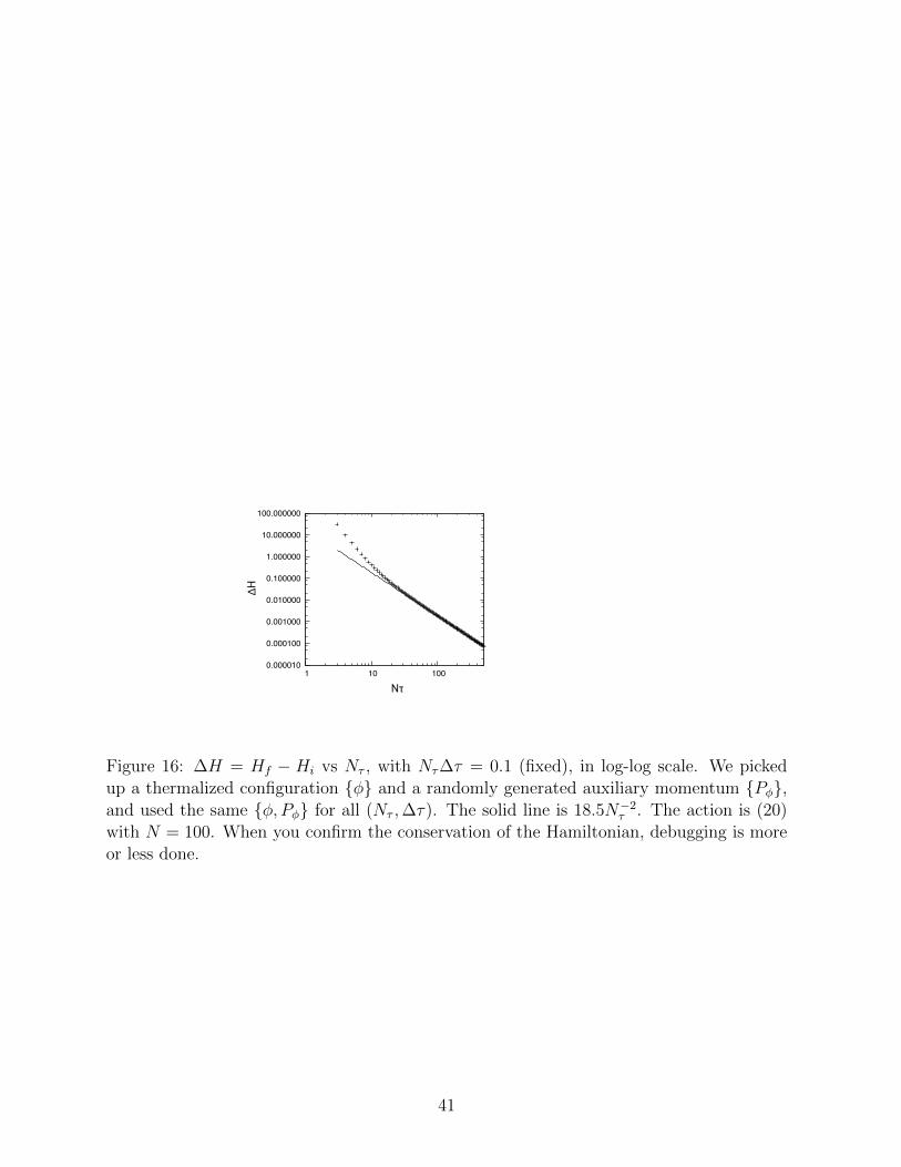
One extra bonus associated with HMC is that we can use the conservation of theHamiltonian for debugging. It is very rare to make bugs in the calculations of the actionand force term consistently; so, practically, unless we code both correctly we cannot see theconservation of the Hamiltonian in the ‘continuum limit’ Nτ → ∞, ∆τ → 0 with Nτ∆τfixed.17 This is a very good check of the code; see Fig. 16.
4.3 Multiple step sizes
Let us conside a two-matrix model
S[φ1, φ2] = NTr (V1(φ1) + V2(φ2) + φ1φ2) , (30)
where
V1(φ1) =m2
1
2φ2
1 +1
4φ4
1, V2(φ2) =m2
2
2φ2
2 +1
4φ4
2. (31)
17 Note that the normalization of the auxiliary momentum and the factor 1/2 at the first and last stepsof the leap-frog evolution cannot be tested by the conservation of the Hamiltonian.
40
0.000010
0.000100
0.001000
0.010000
0.100000
1.000000
10.000000
100.000000
1 10 100
Nτ
ΔH
Figure 16: ∆H = Hf − Hi vs Nτ , with Nτ∆τ = 0.1 (fixed), in log-log scale. We pickedup a thermalized configuration φ and a randomly generated auxiliary momentum Pφ,and used the same φ, Pφ for all (Nτ ,∆τ). The solid line is 18.5N−2
τ . The action is (20)with N = 100. When you confirm the conservation of the Hamiltonian, debugging is moreor less done.
41

Imagine an extreme situation, m1 = 1 and m2 = 1000000000, i.e. φ2 is much heavier.Then typical value of φ1 is much larger than that of φ2. If we use the same step size forboth, then in order to raise the acceptance rate for φ2 we have to take the step size verysmall, which leads to a very long autocorrelation for φ1.
As we have emphasized in Sec. 3.4.2, the choice of the step size has to be consistentwith the requirements listed in Sec. 2, but other than that it is completely arbitrary; seeSec. 4.1. Hence we can simply use different step sizes for φ1 and φ2. This simple fact isvery important in the simulation of QFT: we should use larger step size for lighter particle.Also, in the momentum space, high-frequency modes are ‘heavier’ in that m2 + p2 behaveslike a mass. Hence we should use smaller step size for ultraviolet modes, larger step sizefor infrared modes. This method is called ‘Fourier acceleration’.
4.4 Different algorithms for different fields
We can even use different update algorithms for different variables, and as we will see,this is important when we study systems with fermions.
Let us consider
S(x, y) = y2f(x) + g(x) (32)
where f(x) and g(x) are complicated functions. Then we can repeat the following twosteps,
• Update y for fixed x,
• Update x for fixed y.
In Sec. 4.1 we introduced essentially the same example, namely we adopted the Metropolisalgorithm and varied x1, x2, · · · one by one.
If f(x) > 0, then z ≡ y√f(x) has a Gaussian weight for each fixed x. In this case, we can
use the Box-Muller algorithm (Appendix B) to generate z; then there is no autocorrelationbetween y’s. Hence we can use the following method:
• Update y for fixed x, by generating Gaussian random z and setting y = z/√f(x).
• Update x for fixed y, by using Metropolis or HMC.
Note that the use of the Box-Muller algorithm does not violate the conditions listed inSec. 2. It just gives us a very special Markov chain without autocorrelation.
4.5 QFT example 1: 4d scalar theory
Let us consider 4d scalar theory,
S[φ] = N
∫d4xTr
(1
2(∂µφ)2 +
m2
2φ2 + V (φ)
), (33)
42
where the N×N Hermitian matrices φ(x) now depends on the coordinate x. For simplicitywe assume the spacetime is compactified to a square four-torus with circumference ` andvolume V = `4. It can be regularized by using an n4 lattice with the lattice spacing a = L/nas
Slattice[φ] = Na4∑~x
Tr
(1
2
∑µ
(φ~x+µ − φ~x
a
)2
+m2
2φ2~x + V (φ~x)
), (34)
where µ stands for a shift of one lattice unit along the µ direction. The path-integral is justa multi-variable integral with Hermitian matrices, the methods we have already explainedcan directly be applied.
4.6 QFT example 2: Wilson’s plaquette action (SU(N) pure Yang-
Mills)
Let’s move on to 4d SU(N) Yang-Mills. The continuum action we consider is
Scontinuum =1
4g2YM
∫d4xTrF 2
µν , (35)
where the field strength Fµν is defined by Fµν = ∂µAν−∂νAµ+ i[Aµ, Aν ]. Typically we takethe ’t Hooft coupling λ = g2
YMN fixed when we take large N . As a lattice regularizationwe use Wilson’s plaquette action,18
Slattice = −βN∑µ 6=ν
∑~x
Tr Uµ,~xUν,~x+µU†µ,~x+νU
†ν,~x. (36)
Here Uµ,~x is a unitary variable living on a link connecting to lattice points ~x and ~x + aµ,where a is the lattice spacing and µ is a unit vector along the µ-th direction. It is relatedto the gauge field Aµ(~x) by Uµ,~x = eiaAµ(~x). The lattice coupling constant β is the inverseof the ’t Hooft coupling, β = 1/λ, and it should be scaled appropriately with the latticespacing a in order to achieve the right continuum limit.
4.6.1 Metropolis for unitary variables
The only difference is that, instead of adding random numbers, we should multiplyrandom unitary matrices. A random unitary matrix can be generated as follows. Firstly,we generate random Hermitian matrix H by using random numbers. For example we cangenerate it with Gaussian weight ∼ e−TrH2/2σ2
. Then V = eiH is random unitary centeredaround V = 1. When σ is small, it is more likely to be close to 1. Hence σ is ‘step size’. Ofcourse, you can use the uniform random number to generate H if you want. Regardless,the Metropolis goes as follows:
18 Often the overall factor N is included in β and β′ = βN is used as the lattice coupling. It is simplya bad convention when we consider generic values of N , because the coupling to be fixed as N is varied isnot β′ but β.
43

1. Generate V randomly, change U1,~x to U ′1,~x = U1,~xV , and perform the Metropolis test.
2. Do the same for U2,~x, U3,~x and U4,~x.
3. Do the same for other lattice sites.
4. Repeat the same procedure many many times.
4.6.2 HMC for Wilson’s plaquette action
HMC for unitary variables goes as follows. Let us define the momentum pijµ conjugateto the gauge field Ajiµ by
dU
dτ= ipU,
dU †
dτ= −iUp. (37)
It generates
U → eiδAU, U † → U †e−iδA. (38)
Therefore,
dpijdτ
= − ∂S
dAji= −i
(U∂S
∂U
)ij
+ i
(U∂S
∂U
)∗ji
(39)
where the second term comes from the derivative w.r.t. U †. The discrete molecular evolu-tion can be defined as follows:
1.
U(∆τ/2) = exp
(i∆τ
2p(0)
)· U(0),
p(∆τ) = p(0) + ∆τ · dpdτ
(∆τ/2).
2. Repeat the following for τ = ∆τ, 2∆τ, · · · , (Nτ − 1)∆τ :
U(τ + ∆τ/2) = exp (i∆τp(τ)) · U(τ −∆τ/2),
p(τ + ∆τ) = p(τ) + ∆τ · dpdτ
(τ + ∆τ/2).
3.
U(Nτ∆τ) = exp
(i∆τ
2p(Nτ∆τ)
)· U(
(Nτ − 1/2)∆τ).
In order to calculate ei∆τp, it is necessary to diagonalize p. As long as one considersSU(N) theory with not very large N , the diagonalization is not that costly. (Note also that,when the fermions are introduced, this part cannot be a bottle-neck, so we do not have tocare; we should spend our effort for improving other parts.) In case we need to cut the costas much as possible, we can approximate it by truncating the Taylor expansion of ei∆τ ·p atsome finite order.
44

5 Including fermions with HMC and RHMC
Let us consider the simplest example,
S[x, ψ, ψ] =x2
2+ ψD(x)ψ, (40)
where ψ is a complex Grassmann number and a function D(x) is a ‘Dirac operator’. Wecan integrate out ψ by hand, so that
Z =
∫dxdψdψe−S[x,ψ,ψ] =
∫dxD(x)e−x
2/2 =
∫dxe−x
2/2+logD(x). (41)
Hence we need to deal with the effective action in terms of x, Seff = x2
2− logD(x). This
is simple enough so that we don’t need anything more sophisticated than the Metropolisalgorithm. However our life becomes a bit more complicated when there are multiplevariables, x1,2,··· ,nx and ψ1,2,··· ,nψ . Let us consider the action of the following form,
S[x, ψ, ψ] =nx∑i=1
x2i
2+
nψ∑a,b=1
ψaDab(x)ψb. (42)
Now the Dirac operator Dab(x) is an nψ × nψ matrix, and the partition function becomes
Z =
∫[dx][dψ][dψ]e−S[x,ψ,ψ] =
∫[dx] detD(x) · e−
∑i x
2i /2. (43)
We can still use the Metropolis algorithm in principle,19 but the calculation of the determi-nant is very costly (cost∼ n3
ψ). Even worse, though Dab(x) is typically sparse, it is not easyto utilize the sparseness when one calculates the determinant. HMC and RHMC avoid theevaluation of the determinant and enable us to utilize the sparseness of Dab(x).
5.1 2-flavor QCD with HMC
Let us consider 2-flavor QCD, whose action in the continuum is
S[Aµ, ψf , ψf ] =
∫d4x
(1
4TrF 2
µν +2∑
f=1
ψ(f)D(f)ψ(f)
), (44)
where Aµ(µ = 1, 2, 3, 4) is the SU(3) gauge field and Df = γµDµ+mf is the Dirac operatorwith fermion mass mf . For a lattice regularization, we use link variables as in Sec.4.6, andput fermions on sites. The latice action we consider is
SLattice[Uµ, ψf , ψf ] = SB[Uµ] +∑~x,~y
2∑f=1
ψ(f)~xαD
(f)~xα,~yβψ
(f)~yβ , (45)
19 Here we assumed detD(x) > 0 for any x, i.e. the sign problem is absent.
45
where SB[Uµ] is the plaquette action (36). There are various choices for a lattice Dirac
operator D(f)~xα,~yβ; we do not specify it here.
Below we assume m1 = m2 = m (i.e. neglect the difference of the mass of up and downquarks), then the partition function is
ZLattice =
∫[dU ] (detD)2 e−SB . (46)
Usually the determinant is real, and hence (detD)2 = det(D†D).Now we introduce pseudo-fermion F , on which the Dirac operator acts just in the same
way as on ψ. But F is a complex bosonic field. Then
ZLattice =
∫[dU ][dF ]e−SB−F
†(D†D)−1F . (47)
At first sight it may look like a stupid way of writing an easy thing in a complicated form.However it enables us to avoid the calculation of detD; rather we have to calculate a linearequation
(D†D)χ = F, (48)
for which the sparseness of D can be fully utilized. In order to obtain the solution χ, wecan use the conjugate gradient method; see Appendix A.
The strategy is simply applying the HMC algorithm to
S[Uµ, F ] = SB[Uµ] + F †(D†D)−1F, (49)
by using Aµ and F as dynamical variables. The only nontrivial parts are the calculation ofthe force and Hamiltonian. For that, we only need the solution χ of (D†D)χ = F . Indeed,the force is calculated as
− ∂S
∂Aµ= −∂SB
∂Aµ+ χ†
∂(D†D)
∂Aµχ (50)
and
− ∂S
∂F †= χ, (51)
and the action is simply
S[Uµ, F ] = SB[Uµ] + F †χ. (52)
A better way of treating F
It is possible to update the pseudo-fermion F more efficiently, by using the idea explainedin Sec.4.4. This is based on a simple observation that Φ ≡
(D†)−1
F has the Gaussianweight and hence can easily be generated randomly by using the Gaussian random numbergenerator.
Hence we can do as follows:
46

1. Randomly generate Φ(k+1) with the Gaussian weight20 e−Φ†Φ.
2. Calculate the pseudo-fermion F (k+1) = D†(U(k)µ ) · Φ(k+1).
3. Randomly generate auxiliary momenta P(k)µ , which are conjugate to A
(k)µ , with prob-
abilities proportional to e−Tr(P(k)µ )2/2.
4. Calculate
Hi = SB[U (k)] +∑µ
Tr(P (k)µ )2/2 + (F (k+1))†(D†(U (k)) ·D(U (k)))−1F (k+1). (53)
Note that (F (k+1))†(D†(U (k)) ·D(U (k)))−1F (k+1) = (Φ(k+1))†Φ(k+1).
5. Then perform the Molecular evolution for Uµ, fixing F to be F (k+1). The force is
−∂SB∂Aµ
+ χ†∂(D†D)
∂Aµχ, (54)
where (D†D)χ = F as before. Then we obtain U(k+1)µ and P
(k+1)µ .
6. Calculate
Hf = SB[U (k+1)] +∑µ
Tr(P (k+1)µ )2/2 + (F (k+1))†(D†(U (k+1)) ·D(U (k+1)))−1F (k+1).
(55)
7. Metropolis test: Generate a uniform random number r between 0 and 1. If r < eHi−Hf ,U
(k+1)µ = U
(k)µ (τf ), otherwise U
(k+1)µ = U
(k)µ .
8. Repeat 1–7.
5.2 (2+1)-flavor QCD with RHMC
Strange quark has much bigger mass than up and down quarks. So let us take m1 =m2 m3 = ms. Let us denote the Dirac operators for up and down by D, and the one forstrange by Ds. The partition function is
ZLattice =
∫[dU ] (detDs) (detD)2 e−SB . (56)
20 By using the Box-Muller algorithm explained in Appendix B, real Gaussian random numbers withvariance 1 is generated, i.e. the weight of x, y ∈ R is e−x
2/2 and e−y2/2. By dividing x = x/
√2 and
y = y/√
2 have the weights e−x2
and e−y2
. To reproduce the weight is e−Φ†Φ = e−(ReΦ)2−(ImΦ)2 , we shouldtake Φ = (x+
√−1y) = (x+
√−1y)/
√2. If you use a wrong normalization, you end up in a wrong result.
47

Hence we need to introduce two pseudo fermions F and Fs as21
S[Uµ, F ] = SB[Uµ] + F †(D†D)−1F + F †s (D†sDs)−1/2Fs. (57)
The last term in the right hand side is problematic because it is difficult (or costly) to solve(D†D)1/2χs = Fs.
The Rational Hybrid Monte Carlo (RHMC) algorithm [15] evades this problem by uti-lizing a rational approximation,
(D†D)−1/2 ' a0 +
Q∑i=1
aiD†D + bi
, (58)
where a’s and b’s are positive constants, and Q is typically 10 or 20. These numbers areadjusted so that the rational approximation is good for all samples appearing in the actualsimulation. A good code to find such numbers can be found at [17].
By using this rational approximation, we replace the last term by
Sstrange = a0F†sFs +
Q∑i=1
aiF†s
1
D†sDs + biFs. (59)
To determine the force, we need to solve (D†sDs + βi)χs,i = Fs. Rather surprisingly, wedo not have to solve these equations Q times; the multi-mass CG solver [16] solves all Qequations simultaneously, essentially without any additional cost. See Appendix A.
1. Randomly generate Φ(k+1) and Φ(k+1)s with the Gaussian weights e−Φ†Φ and e−Φ†sΦs .
2. Calculate the pseudo-fermion F (k+1) = D†(U(k)µ ) · Φ(k+1).
3. Calculate the pseudo-fermion F(k+1)s =
(D†(U
(k)µ ) ·D(U
(k)µ ))1/4
Φ(k+1)s . See the end of
this section for an efficient way to do it.
4. Randomly generate auxiliary momenta P(k)µ , which are conjugate to A
(k)µ , with prob-
abilities proportional to e−Tr(P(k)µ )2/2.
5. Calculate
Hi = H[U (k), P (k), F (k+1), F (k+1)s ] (60)
where
H[U, P, F, Fs] = SB[U ] +∑µ
Tr(Pµ)2/2
+F †(D†(U) ·D(U))−1F
21 D†sDs is used so that the action becomes positive definite.
48

+a0F†sFs +
Q∑i=1
aiF†s
1
Ds(U)†Ds(U) + biFs. (61)
Note that, although the last line formally seems to agree with (Φ(k+1)s )†Φ
(k+1)s at τ = 0,
it is not the case due to the approximations used for (D†D)−1/2 and (D†D)+1/4 arenot exactly the ‘inverse’.
6. Then perform the Molecular evolution for Uµ, fixing F to be F (k+1). The force is
−∂SB∂Aµ
+ χ†∂(D†D)
∂Aµχ+
Q∑i=1
aiχ†s,i
∂(D†sDs)
∂Aµχs,i, (62)
where (D†D)χ = F and (D†sDs + bi)χs,i = Fs. Then we obtain U(k+1)µ and P
(k+1)µ .
7. Calculate
Hf = H[U (k+1), P (k+1), F (k+1), F (k+1)s ] (63)
8. Metropolis test: Generate a uniform random number r between 0 and 1. If r < eHi−Hf ,U
(k+1)µ = U
(k)µ (τf ), i.e. the new configuration is ‘accepted.’ Otherwise U
(k+1)µ = U
(k)µ ,
i.e. the new configuration is ‘rejected.’
9. Repeat 1 – 8.
How to calculate F =(D†D
)1/4Φ
We can use the rational approximation
x1/4 ' a′0 +
Q′∑k=1
a′kx+ b′k
. (64)
Then
F ' a′0Φ + a′kχ′k, (65)
where
1
D†sDs + b′kΦ = χ′k (66)
is obtained by solving
(D†sDs + b′k)χ′k = Φ. (67)
We can use the multi-mass solver; see Appendix A.
49

6 Maximal SYM with RHMC
Sec. 6.1 is for lattice people who knows almost nothing about SYM. String theorists,formal QFT people and lattice theorists who already know SYM can skip it.
6.1 The theories
Supersymmetry relates bosons and fermions. Because it changes the spin of the fields, ifthere are too many supercharges (i.e. generators of supersymmetry transformation) higherspin fields have to be involved. In order to construct a gauge theory without gravity, wecannot have massless fields with spin larger than one. It restricts the possible number ofsupercharges: the maximal number is sixteen. The maximally supersymmetric Yang-Millstheories (or maximal SYM) are the supersymmetric generalizations of Yang-Mills theorywith sixteen supercharges. They can be obtained from SYM in (9+1) dimensions as follows.
Firstly, why do we care about (9 + 1) dimensions? It is related to sixteen. In (9 + 1)-dimensional Minkowski space, there is a sixteen-dimensional spinor representation, whichis Majorana and Weyl. Hence the minimal supersymmery transformation has sixteen com-ponents; and as we have seen above, it is maximal as well. The field content is simple:gauge field AM(M = 0, 1, · · · , 9) and its superpartner (gaugino) ψα(α = 1, 2, · · · , 16). Bothof them are N ×N Hermitian matrices. The action is22
S(9+1)-d =1
g2YM
∫d10xTr
(−1
4F 2MM ′ +
i
2ψγMDMψ
), (68)
where FMM ′ = ∂MAM ′ − ∂M ′AM + i[AM , AM ′ ] and DMψ = ∂Mψ + i[AM , ψ]. γM is theleft-handed part of the 10d gamma matrices, which can be chosen as
γ0 = 1⊗ 1⊗ 1⊗ 1,
γ1 = σ3 ⊗ 1⊗ 1⊗ 1,
γ2 = σ2 ⊗ σ2 ⊗ σ2 ⊗ σ2,
γ3 = σ2 ⊗ σ2 ⊗ 1⊗ σ1,
γ4 = σ2 ⊗ σ2 ⊗ 1⊗ σ3,
γ5 = σ2 ⊗ σ1 ⊗ σ2 ⊗ 1,
γ6 = σ2 ⊗ σ3 ⊗ σ2 ⊗ 1,
γ7 = σ2 ⊗ 1⊗ σ1 ⊗ σ2,
γ8 = σ2 ⊗ 1⊗ σ3 ⊗ σ2,
γ9 = σ1 ⊗ 1⊗ 1⊗ 1. (69)
They are all real and symmetric. The fermion ψ is Majorana-Weyl, namely ψ†α = ψα.
22We use (−,+, · · · ,+) signature.
50
Theories in lower spacetime dimensions can be obtained by the dimensional reduction.Let us restrict spacetime to be (p + 1)-dimensional. Namely, we do not allow the fields todepend on xp+1, · · · , x9:
AM(x0, x1, · · · , xp, · · · , x9) = AM(x0, x1, · · · , xp),ψα(x0, x1, · · · , xp, · · · , x9) = ψα(x0, x1, · · · , xp). (70)
Let us use µ, ν, · · · and I, J · · · to denote 0, 1, · · · , p and p + 1, · · · , 9. Also let us use XI
to denote AI . Then
Fµν = ∂µAν − ∂νAµ + i[Aµ, Aν ],
FµI = ∂µXI − ∂IAµ + i[Aµ, XI ] = ∂µXI + i[Aµ, XI ] = DµXI ,
FIJ = ∂IXJ − ∂JXI + i[XI , XJ ] = i[XI , XJ ]. (71)
Here DµXI is the covariant derivative; XI behaves as an adjoint scalar after the dimensionalreduction. Hence the dimensionally reduced theory has the following action:
S(p+1)-d = SB + SF , (72)
where
SB =1
g2YM
∫dp+1xTr
(−1
4F 2µν −
1
2(DµXI)
2 +1
4[XI , XJ ]2
)(73)
and
SF =1
g2YM
∫dp+1xTr
(i
2ψΓµDµψ −
1
2ψΓI [XI , ψ]
). (74)
The Euclidean theory is obtained by performing the Wick rotation:
SEuclidean =1
g2YM
∫dp+1xTr
(1
4F 2µν +
1
2(DµXI)
2 − 1
4[XI , XJ ]2
+1
2ψDtψ +
i
2
3∑µ=1
ψγµDµψ −1
2ψΓI [XI , ψ]
). (75)
6.2 RHMC for SYM
By integrating out the fermions by hand, we obtain the Pfaffian23 of the Dirac operator:
Z =
∫[dA][dX](PfD[A,X]) · e−SB [A,X]. (76)
23 Pfaffian is defined for 2n × 2n antisymmetric matrices M , where n = 1, 2, · · · . Roughly speak-ing, the Pfaffian is the square root of the determinant: (PfM)2 = detM . More precisely, PfM =
12nn!
∑σ∈S2n
sgn(σ)∏ni=1Mσ(2i−1)σ(2i).
51

Unfortunately, PfD is not positive definite. Hence we use the absolute value of the pfaffianinstead:
Zphase quench =
∫[dA][dX]|PfD[A,X]| · e−SB [A,X]. (77)
For the justification of this phase quenching, see Sec. 7.2.In order to evaluate this integral, we use the RHMC algorithm.24 The starting point is
to rewrite |PfD| =(det(D†D)
)1/4as
|PfD| =∫dFdF ∗ exp
(−((D†D)−1/8F )†((D†D)−1/8F )
). (78)
If we define Φ by Φ = (D†D)−1/8F , then Φ can be generated by the Gaussian weight e−Φ†Φ,and F can be obtained by F = D1/8Φ.
We further rewrite this expression by using the rational approximation
x−1/4 ' a0 +
Q∑k=1
akx+ bk
. (79)
Then we can replace the Pfaffian with
|PfD| =∫dFdF ∗ exp (−SPF) , (80)
where
SPF = a0F†F +
Q∑k=1
akF†(D†D + bk)
−1F. (81)
The parameters ak, bk, a′k and b′k are real and positive, and can be chosen so that the
approximation is sufficiently good within the range of D†D during the simulation.Now it is clear that everything is the same as RHMC for strange quark except that the
powers are different. Therefore, the molecular evolution goes as follows:
1. Generate Φ by the Gaussian weight.
2. Calculate F = (D†D)1/8Φ.
3. Calculate Hi.
4. Fix F and update Aµ and XI .
5. Calculate Hf .
24 RHMC has been widely used in lattice QCD. The first application to SYM can be found in [18].
52

6. Do the Metropois test.
Computationally most demanding part is solving the linear equations
(D + bk)χk = F (k = 1, · · · , Q), (82)
which appears in the derivative of SPF ,
∂SPF∂A
= −Q∑k=1
akχ†k
∂D∂A
χk,∂SPF∂X
= −Q∑k=1
akχ†k
∂D∂X
χk. (83)
This is much easier than evaluating the Pfaffian.
7 Difference between SYM and QCD
Let us explain important differences between SYM and QCD simulations.25
7.1 Parameter fine tuning problem and its cure
Symmetry plays important roles in physics. For example, why is the pion so light?Because QCD has approximate chiral symmetry and pion is the Nambu-Goldstone bosonassociated with this symmetry. Finite quark mass breaks chiral symmetry softly, so thata light mass of pion is generated. The Wilson fermion breaks chiral symmetry explicitly.If we use it as a lattice regularization, the radiative corrections generate pion mass, andhence we have to fine-tune the bare quark mass to keep the pion light. This is a well knownexample of the parameter fine tuning problem. This problem does not exist if we use overlapfermion [19] or domain-wall fermion [20].
As another simple example, let us consider the plaquette action (36). It has many exactsymmetries at regularized level:
• Gauge symmetry Uµ,~x → Ω~xUµ,~xΩ†~x+µ, where Ω~x are unitary matrices defined on sites.
• Discrete translation ~x→ ~x+ µ
• 90-degree rotations, e. g. x→ y, y → −x
• Parity x, y, z → −x,−y,−z
• Charge conjugation U → U †
25 This section has large overlap with other review articles I have written in the past, but I include ithere in order to make this article self-contained.
53
The integral measure is taken to be the Haar measure, which respects these symmetries.Therefore the radiative corrections cannot break them: these are the symmetries of thequantum theory.26 What happens if we use a regulator which breaks these symmetries, saya momentum cutoff which spoils gauge symmetry? Then we need counter terms, whosecoefficients are fine tuned, to restore the gauge invariance in the continuum.
So now we know the basic strategy for the lattice simulation of supersymmetric theories— let’s keep supersymmetry exactly on a lattice! But there is a one-sentence proof of a ‘no-go theorem’: because supersymmetry algebra contains infinitesimal translation Qα, Qβ ∼γµPµ, which is explicitly broken on any lattice by construction, it is impossible to keep entirealgebra exactly.
Still, it is not the end of the game. Exact symmetry at the regularized level is sufficient,but it is not always necessary. Sometimes the radiative corrections can be controlled byusing some other symmetries or a part of supersymmetry algebra.
The first breakthrough emerged for 4d N = 1 pure SYM. For this theory, the supersym-metric continuum limit is realized if the gaugino mass is set to zero. This can be achievedif the chiral symmetry is realized on lattice [21, 22]. Of course it was not really a ‘solu-tion’ at that time, due to the Nielsen-Ninomiya no-go theorem [23]. Obviously, that theauthor of [21] proposed a way to circumvent the no-go theorem [20] was not a coincidence.(Note that the one-parameter fine tuning can be tractable in this case. See [24] for recentdevelopments.)
The second breakthrough was directly motivated by the gauge/gravity duality [25].27
The duality relates supersymmetric theories in various spacetime dimensions, includingthe ones with less than four dimensions, to string/M-theory [27]. Some prior proposals[6, 7, 29, 30] related lower dimensional theories to quantum gravity as well. Because Yang-Mills in less than four dimensions are super-renormalizable, possible radiative correctionsare rather constrained. In particular, in two dimensions, supersymmetric continuum limitcan be guaranteed to all order in perturbation theory by keeping some supersymmetries ina clever manner [26].
Yet another breakthrough came from superstring theory. Maximally supersymmet-ric Yang-Mills in (p + 1) dimensions describe the low-energy dynamics of Dp-branes [31].Furthermore higher dimensional D-branes can be made by collecting lower dimensionalD-branes [32]. In terms of gauge theory, higher dimensional theories can be obtained asspecific vacua of lower dimensional large-N theories. Or in other words, spacetime emergesfrom matrix degrees of freedom [33].
Based on these ideas, various regularization methods have been invented. A list ofregularization schemes for 4-, 8- and 16-SUSY theories without additional matter (i.e.dimensional reductions of 4d, 6d and 10d N = 1 pure super Yang-Mills) is shown below.
26 In this case, discrete translation and rotation symmetries guarantee the invariance under continuoustransformations in the continuum limit.
27 D. B. Kaplan and M. Unsal told me that their biggest motivation was in the gauge/gravity duality.For several years this motivation has not been widely shared among the followers, probably because theydid not mention it explicitly in their first paper [26].
54

For more details see [34] and references therein.
Dimensions # of SUSY Regularization scheme Fine tuning
0+1 4,8,16 lattice none
0+1 4,8,16 momentum cutoff none
1+1 4,8,16 lattice none
2+1 4,8,16 lattice necessary
2+1 4,8 (large-N) fuzzy sphere none
2+1 16 fuzzy sphere none
3+1 4 lattice none
3+1 8,16 lattice necessary
3+1 8 (large-N) lattice + fuzzy sphere none
3+1 16 lattice + fuzzy sphere none
3+1 4,8,16 (large-N) Eguchi-Kawai reduction none
7.2 Sign problem and its cure
A crucial assumption of MCMC is that the path-integral weight e−S is real and positive;otherwise it is not ‘probability’. This condition is often broken. The simplest example isthe path-integral in Minkowski space — the weight eiS, where S is real, is complex. Onemay think this problem is gone in Euclidean space; the life is not that easy, the actionS can be complex after the Wick rotation; it only has to satisfy the reflection positivity,which is the counterpart of the reality in Minkowski space. Well-known evils which causethe sign problem include the θ-term and the Chern-Simons term in Yang-Mills theory, andQCD with finite baryon chemical potential. Note that, although it is often called ‘fermionsign problem’, the source of the sign is not necessary the fermionic part.
Maximal super Yang-Mills have the sign problem, because the pfaffian can take complexvalues.
There is no known generic solution of the sign problem. It has been argued that the signproblem is NP-hard [35], and hence, unless you have a reason to think P=NP, it is a wasteof time to invest your time in searching for a generic solution. However, theory-specificsolutions are not excluded. Probably the best case scenario is that somebody comes upwith a clever change of variables so that the sign problem disappears. I actually had sucha lucky experience when he studied the ABJM matrix model in Ref. [4], thanks to smartstudents who knew important analytic formulas developed in [36]. Certain supersymmetrictheories seem to allow yet another beautiful solution, as we will explain below.
7.2.1 Phase reweighting
Let us consider SYM as a concrete example. The expectation value of an observable O,which is written in terms of Aµ and XI , with the ‘full’ partition function (76) is
〈O(A,X)〉full =
∫[dA][dX](PfD[A,X]) · e−SB [A,X] · O(A,X)∫
[dA][dX](PfD[A,X]) · e−SB [A,X]. (84)
55

By writing PfD = |PfD|eiθ, we can easily see
〈O(A,X)〉full =〈O(A,X) · eiθ[A,X]〉phase quench
〈eiθ[A,X]〉phase quench
, (85)
where 〈 · 〉phase quench is the expectation value with the phase quenched path-integral (77).By using this trivial identity, in principle we can calculate the expectation value in the fulltheory. This method is called phase reweighting.
However there are several reasons we do not want to use the phase reweighting method.Firstly, calculation of the pfaffian is numerically very demanding, and although we can avoidexplicit evaluation of the Pfaffian in the configuration generation with the phase quenchedensemble, in order to calculate (85) we must calculate the Pfaffian explicitly. Secondly, ifthe phase factor eiθ fluctuates rapidly, both the denominator and numerator becomes verysmall, and numerically it is difficult to distinguish them from zero. Then the expression ispractically 0/0, whose error bar is infinitely large. The fluctuation is particularly violentwhen the full theory and phase quenched theory does not have substantial overlap (seeSec. 3.3.1), and it actually happens in finite density QCD. As we will argue shortly, thefull theory and phase quenched theory are rather close in the case of SYM. Still, the phasefluctuation is very large and it is impossible to calculate the average phase at large Nand/or large volume. Roughly speaking, θ is the imaginary part of the action, which scalesas N2 times volume!
Although the phase reweighting is an unrealistic approach to SYM, it can be a practicaltool when the simulation cost is cheaper. For example it is a common strategy in certainarea of condensed matter physics.
7.2.2 Phase quench
Let us consider the phase quench approximation. Namely, we calculate 〈O(A,X)〉phase quench,which does not take into account the phase at all, instead of 〈O(A,X)〉full. Such an ‘ap-proximation’ can make sense when O and eiθ factorize, 〈Oeiθ〉phase quench ' 〈O〉phase quench×〈eiθ〉phase quench.
The phase quench approximation almost always fails. Very fortunately, rare exceptionsinclude SYM. Firstly, at high temperature and not so large N , θ is close to zero andhence the phase can safely be ignored. Rather surprisingly, θ remains small down to ratherlow temperature and moderately large N , which is relevant for testing the gauge/gravityduality; see e.g. [37, 38, 39, 40, 41] for explicit checks for (0 + 1)- and (1 + 1)-dimensionaltheories. At low temperature or with supersymmetric boundary condition, the phase factordoes oscillate. Still, as long as the fluctuation is not very rapid, we can defeat the signby brute force. Then we can confirm 〈O〉phase quench = 〈O〉full within numerical error, forsome observables [40, 42]. When the phase factor fluctuates rapidly, or the dimension ofthe Dirac operator is too big, we cannot evaluate the effect of the phase. Still we can makean indirect argument based on numerical evidence that the phase quench approximation isgood for certain observables [43].
56
Note that the phase quench leads to a wrong result for the type IIB matrix model [28],which is the dimensional reduction of maximal SYM to zero dimension.
7.3 Flat direction and its cure
Many supersymmetric Yang-Mills theories (practically all theories relevant in the contextof the gauge/gravity duality) have adjoint scalar fields XI . There are flat directions alongwhich scalar matrices commute, [XI , XJ ] = 0, and the eigenvalues roll to infinity. With2 or 3 noncompact spatial dimensions, we can fix the eigenvalues by hand; it is a choiceof moduli, due to the superselection. However with compact space28 or lower dimensionsthe eigenvalue distribution should be determined dynamically. There is nothing wrong withthis: the flat direction is a feature of the theory, it is not a bug. However it causes headachewhen we perform MCMC for two reasons: firstly, the partition function is not convergent,and hence the simulation never thermalizes [37]. Secondly, when the eigenvalues roll toofar, the lattice simulation runs into an unphysical lattice artifact [44].
In order to tame the flat directions, we have to understand its physical meaning. (p+1)-dU(N) SYM describe a system of N Dp-branes sitting parallel to each other, and the eigen-values (X ii
1 , Xii2 , · · · , X ii
9−p) describe the location of the i-th Dp-brane. When eigenvaluesform a bound state, it can be regarded as a black p-brane. When one of the eigenvalues isseparated far from others, the interaction is very weak due to supersymmetry; the potentialis proportional to −f(T )/r8−p [45, 46], where r is the distance, T is temperature of theblack brane and f(T ) is a monotonically increasing function which vanishes at T = 0. Thispotential is not strong enough to trap a Dp-brane once it is emitted from the black brane.In the same manner, phases with multiple bunches of eigenvalues can exist; they describemultiple black branes. This is the reason that the flat directions exist; the partition functionis not convergent because there are too many different classes of configurations.
Now our task is apparent: we should cut out configurations describing certain physi-cal situation we are interested. The first thing we should study is a single black hole orblack brane, namely a bound state of all eigenvalues. This bound state is only metastable,but as N increases it becomes stable enough so that we can collect sufficiently many con-figurations without seeing the emission of the eigenvalues [37]. Large-N behavior of the(0 + 1)-dimensional theory has been studied in this manner in [37, 38, 43]. When N issmall, we need to introduce a cutoff for the eigenvalues. In [47] a cutoff is introduced for(1/N)
∑M TrX2
M , and by carefully changing the cutoff the property of the single bunchphase has been extracted. It is also possible to introduce a mass term Nm2
∫dp+1xTrX2
M
and take m → 0 [48, 44]. Note that one has to make sure that the flat direction is undercontrol when m2 is small, as demonstrated in [48, 44], because simulations often pick up theflat direction and end up in the U(1)N vacuum. See also [49, 50][51, 52, 53, 41][54] for thedetails on how to control the flat directions in actual simulations. It is also possible to addslightly more complicated deformation which preserves (at least a part of) supersymmetry,
28 More precisely, the torus compactification. For the compactification to a curved manifold, the flatdirections are lifted by a mass term associated with the curvature.
57
which is so-called ‘plane wave deformation’ [55]. See [55, 56] for various (0 + 1)-d theoriesand [57, 58, 59] for (1 + 1)-d lattice construction. See also [60] for other cases.
8 Conclusion
In this article I have tried to explain the essence of Markov Chain Monte Carlo. Simplealgorithms like the Metropolis algorithm is good enough for solving nontrivial problems inhep-th literature on a laptop.
Serious simulations of super Yang-Mills require more efforts, but the basic idea is thesame. We just have to update the configurations more efficiently. For that, we can useefficient techniques developed in lattice QCD community: HMC, RHMC and many morewhich I haven’t explained in this article. They can be implemented to our simulationcode by using +,−,×,÷, sin, cos, exp, log,
√, “if” and loop. There are some challenging
issues specific to supersymmetric theories, most notably the problem associated with flatdirections, but we already know basic strategies to handle them.
In this article I did not explain the complete details of lattice SYM simulation. Thedetail of the simulations of BFSS matrix model can be found in the article available at [8].
Acknowledgement
I thank Tatsuo Azeyanagi, Valentina Forini, Anosh Joseph, Michael Kroyter, So Mat-suura, R. Loganayagam, Joao Penedones, Enrico Rinaldi, David Schaich, Masaki Tezukaand Toby Wiseman. I was in part supported by JSPS KAKENHI Grants 17K14285. Manymaterials in this article were prepared for “Nonperturbative and Numerical Approachesto Quantum Gravity, String Theory and Holography”, which was held from 27 January2018 to 03 February 2018 at International Center for Theoretical Science. I thank AnoshJoseph and R. Loganayagam for giving me that wonderful opportunity. This work was alsopartially supported by the Department of Energy, award number de-sc0017905.
A Multi-mass CG method
A.1 (Single-mass) CG method
Let us first introduce the ordinary (or ‘single-mass’) conjugate gradient method. Thenotation is that of [61]. We want to solve the linear equation
A~x = ~b, (86)
where A = D†D. We construct a sequence of approximate solutions ~x1, ~x2, · · · which(almost always) converges to the solution.
58

We start with an initial trial solution ~x1, which is arbitrary. From this we define~r1, ~r1, ~p1, ~p1 as
~r1 = ~r1 = ~p1 = ~p1 = ~b− A~x1. (87)
Then, we construct ~xk as follows:
1. αk =~r†k·~rk~p†k·A~pk
.
2. ~xk+1 = ~xk + αk~pk.
3. ~rk+1 = ~rk − αkA~pk.
4. βk =~r†k+1·~rk+1
~r†k·~rk.
5. ~pk+1 = ~rk+1 + βk~pk.
Note that ~rk = ~b−A~xk. The norm of ~rk converges to zero, or equivalently, ~xk convergesto the solution.
A.2 Multi-mass CG method
Let Aσ be ‘shifted’ version of A:
Aσ = A+ σ · 1. (88)
If A were the Laplacian, σ would be interpreted as a mass term. The multi-mass CG solver[16] enables us to solve Aσ~x = ~b for many different values of σ simultaneously, with onlynegligibly small additional cost.
The key idea is that, from the iterative series for A,
~rk+1 = ~rk − αkA~pk,~pk+1 = ~rk+1 + βk~pk, (89)
it is possible to construct a similar series for the shifted operator,
~rσk+1 = ~rσk − ασkAσ~pσk ,~pσk+1 = ~rσk+1 + βσk ~p
σk , (90)
where
~rσk = ζσk~rk. (91)
59

Indeed, (90) can be satisfied by taking29
ασk = αk ·ζσk+1
ζσk,
βσk = βk ·(ζσk+1
ζσk
)2
,
ζσk+1 =ζσk ζ
σk−1αk−1
αk−1ζσk−1(1 + αkσ) + αkβk−1(ζσk−1 − ζσk ). (93)
Therefore, we can generalize the usual BiCG solver in the following manner:
1. αk =~r†k·~rk~p†k·A~pk
.
2. Calculate ζσk+1 and ασk using (93).
3. ~xσk+1 = ~xσk + ασk~pσk .
4. ~rk+1 = ~rk − αkA~pk.
5. βk =~r†k+1·~rk+1
~r†k·~rk.
6. Calculate βσk using (93).
7. ~pk+1 = ~rk+1 + βk~pk,
~pσk+1 = ~rσk+1 + βσk ~pσk .
Then, ~xσk is an approximate solution with the residual vector ~rσk ,
~rσk = ~b− Aσ~xσk . (94)
Note that we cannot start with an arbitrary initial condition, because (90) is not satisfiedthen. We choose the following special initial condition in order to satisfy (90):
~x1 = ~xσ1 = ~p0 = ~pσ0 = ~0,
~r1 = ~rσ1 = ~r0 = ~rσ0 = ~p1 = ~pσ1 = ~b,
ζσ0 = ζσ1 = α0 = ασ0 = β0 = βσ0 = 1. (95)
As long as we stick to this initial condition, it is hard to implement any preconditioning.If you know any preconditioning which can be used with multi-mass CG solver, please letus know.
29 From (89) we have
~rk+1 =
(1 +
αkβk−1
αk−1
)~rk − αkA~rk −
αkβk−1
αk−1~rk−1. (92)
Comparing the coefficients with those in a similar equation obtained from (90), we obtain (93).
60

B Box-Muller method
Let p and q be uniform random numbers in [0, 1]. There are many random number genera-tors which give you such p and q. Then, x =
√−2 log p sin(2πq) and y =
√−2 log p cos(2πq)
are random numbers with weights e−x2/2
√2π
and e−y2/2
√2π
.
C Jackknife method: generic case
In Sec. 3.2.1, we assumed that a quantity of interest can be calculated for each sample.Let us consider more generic cases; for example in order to determine the mass of particleexcitation we need to calculate two-point function by using many samples and then extractthe mass from that, and hence the mass cannot be calculated sample by sample.
In the Jackknife method, we first divide the configurations to bins with width w; thefirst bin is x(1), x(2), · · · , x(w), the second bin is x(w+1), x(w+2), · · · , x(2w), etc.Suppose we have n bins. Then we define the average of an observable f(x) with k-th binremoved,
f(k,w) ≡ (the value calculated after removingk-th bin) . (96)
The average value is defined by
f ≡ 1
n
∑k
f(k,w)
. (97)
The Jackknife error is defined by
∆w ≡√n− 1
n
∑k
(f
(k,w) − f)2
. (98)
References
[1] J. Penedones, private communication.
[2] T. Azeyanagi, M. Hanada, T. Hirata and T. Ishikawa, JHEP 0801, 025 (2008)[arXiv:0711.1925 [hep-lat]].
[3] T. Azeyanagi, M. Hanada, M. Unsal and R. Yacoby, Phys. Rev. D 82, 125013 (2010)[arXiv:1006.0717 [hep-th]].
[4] M. Hanada, M. Honda, Y. Honma, J. Nishimura, S. Shiba and Y. Yoshida, JHEP 1205,121 (2012) doi:10.1007/JHEP05(2012)121 [arXiv:1202.5300 [hep-th]].
[5] http://www.netlib.org/lapack/
61

[6] T. Banks, W. Fischler, S. H. Shenker and L. Susskind, Phys. Rev. D 55, 5112 (1997)[hep-th/9610043].
[7] B. de Wit, J. Hoppe and H. Nicolai, Nucl. Phys. B 305, 545 (1988).
[8] M. Hanada, A simulation code written for Monte Carlo String/M-theory Collaboration,freely available at https://sites.google.com/site/hanadamasanori/home/mmmm
[9] D. Schaich and T. DeGrand, Comput. Phys. Commun. 190, 200 (2015) [arXiv:1410.6971[hep-lat]].
[10] D. Schaich, Codes for supersymmetric lattice gauge theories ,https://github.com/daschaich/susy
[11] S. Catterall and A. Joseph, Comput. Phys. Commun. 183, 1336 (2012)[arXiv:1108.1503 [hep-lat]].
[12] Metropolis, N., Rosenbluth, A. W., Rosenbluth, M. N., Teller, A. H., and Teller,E. (1953). Equation of state calculations by fast computing machines. The journal ofchemical physics, 21(6), 1087-1092.
[13] O. Aharony, O. Bergman, D. L. Jafferis and J. Maldacena, JHEP 0810, 091 (2008)[arXiv:0806.1218 [hep-th]].
[14] S. Duane, A. D. Kennedy, B. J. Pendleton and D. Roweth, Phys. Lett. B 195, 216(1987).
[15] M. A. Clark and A. D. Kennedy, “The RHMC algorithm for 2 flavors of dynamicalstaggered fermions,” Nucl. Phys. Proc. Suppl. 129, 850 (2004) [arXiv:hep-lat/0309084].
[16] B. Jegerlehner, “Krylov space solvers for shifted linear systems,” arXiv:hep-lat/9612014.
[17] M.A. Clark and A.D. Kennedy,https://github.com/maddyscientist/AlgRemez
[18] S. Catterall and T. Wiseman, JHEP 0712, 104 (2007) [arXiv:0706.3518 [hep-lat]].
[19] H. Neuberger, Phys. Lett. B 417, 141 (1998) [hep-lat/9707022].
[20] D. B. Kaplan, Phys. Lett. B 288, 342 (1992) [hep-lat/9206013].
[21] D. B. Kaplan, Phys. Lett. B 136, 162 (1984).
[22] G. Curci and G. Veneziano, Nucl. Phys. B 292, 555 (1987).
[23] H. B. Nielsen and M. Ninomiya, Nucl. Phys. B 185, 20 (1981) Erratum: [Nucl. Phys.B 195, 541 (1982)]. doi:10.1016/0550-3213(81)90361-8, 10.1016/0550-3213(82)90011-6
62

[24] S. Ali, G. Bergner, H. Gerber, P. Giudice, I. Montvay, G. Mnster, S. Piemonte andP. Scior, JHEP 1803, 113 (2018) [arXiv:1801.08062 [hep-lat]].
[25] J. M. Maldacena, Int. J. Theor. Phys. 38, 1113 (1999) [Adv. Theor. Math. Phys. 2,231 (1998)] [hep-th/9711200].
[26] D. B. Kaplan, E. Katz and M. Unsal, JHEP 0305, 037 (2003) [hep-lat/0206019].
[27] N. Itzhaki, J. M. Maldacena, J. Sonnenschein and S. Yankielowicz, Phys. Rev. D 58,046004 (1998) [hep-th/9802042].
[28] N. Ishibashi, H. Kawai, Y. Kitazawa and A. Tsuchiya, Nucl. Phys. B 498, 467 (1997)[hep-th/9612115].
[29] L. Motl, hep-th/9701025.
[30] R. Dijkgraaf, E. P. Verlinde and H. L. Verlinde, Nucl. Phys. B 500, 43 (1997) [hep-th/9703030].
[31] E. Witten, Nucl. Phys. B 460, 335 (1996) [hep-th/9510135].
[32] R. C. Myers, JHEP 9912, 022 (1999) [hep-th/9910053].
[33] Probably the first demonstration of this philosophy was in T. Eguchi and H. Kawai,Phys. Rev. Lett. 48, 1063 (1982).
[34] M. Hanada, Int. J. Mod. Phys. A 31, no. 22, 1643006 (2016) [arXiv:1604.05421 [hep-lat]].
[35] M. Troyer and U. J. Wiese, Phys. Rev. Lett. 94, 170201 (2005) [cond-mat/0408370].
[36] A. Kapustin, B. Willett and I. Yaakov, JHEP 1010, 013 (2010) [arXiv:1003.5694 [hep-th]].
[37] K. N. Anagnostopoulos, M. Hanada, J. Nishimura and S. Takeuchi, “Monte Carlostudies of supersymmetric matrix quantum mechanics with sixteen supercharges at finitetemperature,” Phys. Rev. Lett. 100, 021601 (2008) [arXiv:0707.4454 [hep-th]].
[38] M. Hanada, Y. Hyakutake, J. Nishimura and S. Takeuchi, Phys. Rev. Lett. 102, 191602(2009) [arXiv:0811.3102 [hep-th]].
[39]
[39] V. G. Filev and D. O’Connor, “The BFSS model on the lattice,” arXiv:1506.01366[hep-th].
[40] M. Buchoff, M. Hanada and S. Matsuura, unpublished.
63

[41] S. Catterall, R. G. Jha, D. Schaich and T. Wiseman, arXiv:1709.07025 [hep-th].
[42] M. Hanada, J. Nishimura, Y. Sekino and T. Yoneya, JHEP 1112, 020 (2011)[arXiv:1108.5153 [hep-th]].
[43] E. Berkowitz, E. Rinaldi, M. Hanada, G. Ishiki, S. Shimasaki and P. Vranas, Phys.Rev. D 94, no. 9, 094501 (2016) [arXiv:1606.04951 [hep-lat]].
[44] M. Hanada and I. Kanamori, JHEP 1101, 058 (2011) [arXiv:1010.2948 [hep-lat]].
[45] U. H. Danielsson, G. Ferretti and B. Sundborg, Int. J. Mod. Phys. A 11, 5463 (1996)[hep-th/9603081].
[46] D. N. Kabat and P. Pouliot, Phys. Rev. Lett. 77, 1004 (1996) [hep-th/9603127].
[47] M. Hanada, Y. Hyakutake, G. Ishiki and J. Nishimura, Science 344, 882 (2014)[arXiv:1311.5607 [hep-th]].
[48] M. Hanada and I. Kanamori, Phys. Rev. D 80, 065014 (2009) [arXiv:0907.4966 [hep-lat]].
[49] S. Catterall, A. Joseph and T. Wiseman, JHEP 1012, 022 (2010) [arXiv:1008.4964[hep-th]].
[50] E. Gigure and D. Kadoh, JHEP 1505, 082 (2015) [arXiv:1503.04416 [hep-lat]].
[51] S. Catterall, P. H. Damgaard, T. Degrand, R. Galvez and D. Mehta, JHEP 1211, 072(2012) [arXiv:1209.5285 [hep-lat]].
[52] S. Catterall, D. Schaich, P. H. Damgaard, T. DeGrand and J. Giedt, Phys. Rev. D 90,no. 6, 065013 (2014) [arXiv:1405.0644 [hep-lat]].
[53] S. Catterall and D. Schaich, JHEP 1507, 057 (2015) [arXiv:1505.03135 [hep-lat]].
[54] D. August, B. H. Wellegehausen and A. Wipf, arXiv:1802.07797 [hep-lat].
[55] D. E. Berenstein, J. M. Maldacena and H. S. Nastase, JHEP 0204, 013 (2002) [hep-th/0202021].
[56] N. Kim and J. H. Park, Nucl. Phys. B 759, 249 (2006) [hep-th/0607005].
[57] M. Hanada, S. Matsuura and F. Sugino, Prog. Theor. Phys. 126, 597 (2011)[arXiv:1004.5513 [hep-lat]].
[58] M. Hanada, JHEP 1011, 112 (2010) [arXiv:1009.0901 [hep-lat]].
[59] M. Hanada, S. Matsuura and F. Sugino, Nucl. Phys. B 857, 335 (2012)[arXiv:1109.6807 [hep-lat]].
64

[60] J. Kato, Y. Kondo and A. Miyake, JHEP 1109, 019 (2011) [arXiv:1104.1252 [hep-th]].
[61] W. H. Press, B. P. Flannery, S. A. Teukolsky and W. T. Vetterling, “Numerical Recipesin FORTRAN, ” Cambridge University Press.
65