marketing spending and customer lifetime value for firms with
TRANSCRIPT
Submitted to Marketing Sciencemanuscript (Please, provide the mansucript number!)
Marketing Spending and Customer Lifetime Value forFirms with Limited Capacity
Anton Ovchinnikov and Phillip E. PfeiferDarden Graduate School of Business, University of Virginia, 100 Darden Blvd., Charlottesville, VA 22903 USA
[email protected], [email protected]
The concept of customer lifetime value (CLV) is widely used by marketing practitioners and academics inmaking decisions about customer acquisition and retention spending. The traditional view of CLV, however,assumes that the firm has the unlimited capacity to serve all its acquired and retained customers. In thispaper we consider a firm with limited capacity and determine the role that CLV plays in its acquisition andretention spending decisions.
We find that the optimal spending for the firm with limited capacity increases in capacity and decreasesin the number of customers. This stands in contrast to the firm with unlimited capacity that spends theCLV-maximizing amount regardless of the number of other customers. Surprisingly, however, the firm withlimited capacity may spend more than the CLV-maximizing amount, which happens when the time value ofmoney is large. When the time value of money is small, the two spending levels are nearly identical whenthe firm is well under capacity, but as the firm grows and approaches its capacity limit, optimal acquisitionand retention spending decrease to substantially lower, but still non-zero levels. We characterize optimalspending for the firm at capacity in closed form and discuss the role CLV plays in optimizing customer mix.
We also examine customer selection decisions. We again find that CLV alone does not determine thosedecisions. In particular, we show the firm with limited capacity may prefer a customer with a lower CLV.
Lastly, we consider capacity expansion. We show that the expansion decision is of the threshold type:intuitively, the firm should expand when it becomes large enough. Interestingly, however, the value of expan-sion is largest when the firm still has significant unutilized capacity. CLV again offers little guidance indetermining this value – per unit value of expanded capacity is much larger than the CLV of the customerwho will occupy it. We also observe an interesting behavior of spending during the timelag between thedecision to expand and the period when the additional capacity becomes operational: in that timelag thefirm drastically reduces spending on the low-value customers, while increasing the spending on the high-valueones in order to rebalance its customer mix in anticipation of additional capacity.
1. IntroductionThe suggestion to view customer relationships as assets that generate cash flows over time datesback to Bursk (1966). Bursk’s proposal to use the “investment value” of a customer to guidemarketing spending decisions is the key idea behind the concept now commonly referred to ascustomer lifetime value (CLV). Defined for our purposes as the present value of the future cashflows attributed to the customer relationship, CLV is a measure that is commonly used to guideboth acquisition and retention marketing spending. Attention directed toward CLV shifts the focusof marketing from transactions to relationships and underlines modern customer relationship man-agement (CRM).
A typical CRM-focused firm will choose its marketing spending so as to maximize separatelythe CLV of each customer. Such CLV-maximizing spending (defined in more detail in Section 4.1)is optimal when the firm has independent relationships with its customers; i.e., when acquiring(retaining) one customer does not affect the cash flows from any of the firm’s other current andfuture customers/prospects.
It is rather obvious, however, that CLV-maximizing spending is suboptimal whenever there existdependencies among customer relationships. Demand-side dependencies, such as customer networkeffects, are well recognized, e.g., Pfeifer (1999), Hogan et al. (2003), and Kumar et al. (2007). Incontrast, supply side dependencies, have received only limited attention in the CRM literature.
1
Ovchinnikov and Pfeifer: Marketing Spending and CLV for Firms with Limited Capacity2 Article submitted to Marketing Science; manuscript no. (Please, provide the mansucript number!)
Berger and Bechwati (2001) discuss the supply side dependency caused by the limited promotionalbudget per person in every time period. Liu et al. (2007) discuss the case in which a limitedsalesforce capacity is available to a single customer over multiple time periods. In general, thereare a variety of supply-side dependencies that make CLV-maximizing spending suboptimal, Pfeiferand Ovchinnikov (2010). The focus of this paper is on a very fundamental form of supply-sidedependency – the case when the number of customers that the firm can serve is limited by someN , to which we refer as the capacity constraint.
Capacity constraints are a reality for many CRM-focused businesses. Capacity limit can be phys-ical if the firm simply cannot serve more than some N customers. Performing arts companies,apartment buildings, sports venues, some colleges, and the like face constraints of this kind. Acapacity limit can also be strategic, when firms for which quality of service depends on the numberof customers served because of queueing or “crowding” (restaurants, health-clubs, medical prac-tices, delivery companies, etc.) strategically limit the number of customers they serve. For exampleKowalczyk (2006) reports the case of a hospital that “shuts doors to new patients.” In either case,capacity constrained CRM-focused firms face a major disconnect: the set of policies that are com-monly applied to capacity constrained firms, such as the revenue management tools employed byairlines, focus on short-term profitability of sales transactions typically at the expense of customerrelationships, while the “typical” CRM policies are designed to maximize separately the value ofeach relationship, and thus ignore capacity constraints. The goal of our paper is to address thisdisconnect.
A capacity constraint is fundamentally different from other types of limited resources, in par-ticular those mentioned above, along at least three dimensions. First, capacity constraint is oftenpractically impossible to remove, e.g., the Green Bay Packers, a professional football team in theU.S., has 81,000 names on its wait list for season tickets with an average wait of 30 years, butno apparent plans to move to a different stadium1. Similarly, several months prior to the startof its 2010 season Opera Company C (name disguised for confidentiality) was sold out in 9 of 14seating areas, and expansion was not an option either2. We refer to such cases as the hard capacityconstraints.
Second, even when capacity can be expanded, doing so is typically discrete and discontinuous(“lumpy”): expansion involves a onetime and usually large fixed cost, which brings the capacity upby some usually large number of units, possibly with some time lag. We refer to such cases as thesoft capacity constraints; restaurants, medical clinics, sports clubs, and the like face constraints ofthis kind. This discreteness contrasts drastically with sales force or marketing budgets: both canbe increased effectively continuously and involve no fixed costs. For example, it is reasonable thata firm might increase its marketing budget by 3%, but if a doctor’s office moves (to expand), thena 3% capacity increase is inconceivable; a far more likely scenario is that they will add, say 30%capacity, even though initially some of this newly added capacity can be idle3. In addition, it is notclear that such continuous forms of limited resources as budget constraints should even be treatedas constraints in the first place: e.g., if the cost of funds is properly accounted for in the cost ofservicing the customer, then the problem reduces to unconstrained CLV maximization. That is
1 http://www.packers.com/fan zone/faq/
2 That is, theoretically and eventually the company may move to a different building, but that decision depends onmany factors (availability of physical space for construction - a major issue in a large metropolis, major (tens ofmillions of dollars) donations, similar size government support, artistic needs, etc.), which by far outweigh CRM inmaking the expansion decision. Thus, when C makes its CRM decisions, it treats the number of seats in the buildingas a constraint now and in the foreseeable future.
3 This adds another, less critical distinction: somewhat unfortunately budgets rarely get underspent, managers areafraid to end up with unused funds, thinking that this will jeopardize future budget allocations; temporarily under-utilized capacity, however, is rather typical.
Ovchinnikov and Pfeifer: Marketing Spending and CLV for Firms with Limited CapacityArticle submitted to Marketing Science; manuscript no. (Please, provide the mansucript number!) 3
not the case with capacity constraint: even if the variable costs of capacity is accounted for in thecontribution margin, the fixed cost cannot be generally allocated to individual customers a prioribecause their number changes over time.
The third, and perhaps the most fundamental difference, is that in the above mentioned papersthe firm was still maximizing individual’s CLV (with the complications introduced by the per-person budget or per-person salesforce limitations). A capacity constraint requires a fundamentallydifferent framework: one in which the firm must realize that “[i]f demand exceeds capacity at anytime, then an opportunity [here, to sell the product/service] is lost”, Rust and Chung (2006). Thiscreates a non-trivial cross-customer and inter-temporal endogeneity, to address which one shouldnot just maximize CLV of every individual separately. Customers are no longer the limited resource– the capacity to serve them is, and thus the firm must operate such as to extract maximum valuefrom its capacity, not necessarily its customers.
Building a model that accounts for the above endogeneities responds well to Rust and Chung’ssuggestion that “we need a model with the following characteristics:” (1) personalized marketinginterventions, (2) multiple interventions, (3) maximizes CLV4, (4) addresses endogeneity. Theyalso point out that “a model that puts all of these elements together” is “missing.” Sun (2006)further develops Rust and Chung’s argument by suggesting that “[f]or a firm with the goal ofmaximizing long-term profit, CRM should be formulated as a stochastic dynamic control problemunder demand uncertainty with the firm as the decision maker which makes dynamic marketingintervention decisions.”
Our paper provides a start at addressing all of the above mentioned concerns. The firm in ourdynamic programming model maximizes its total net present value of the profits from sales toheterogenous customers over an infinite time horizon (following the typical dynamic programmingterminology we refer to this value as the profit-to-go). In each period the firm observes the numberof customers of different types, and decides on the personalized retention spending directed towardeach customer during that period. Such spending reduces the current period’s profit, but increasesthe chance that the customer will be retained next period. In addition to this customer-specificretention spending the firm also decides on acquisition spending for the period; such spending(e.g., on advertising in broadcast media) generates a mixture of new (candidate, potential, etc.)customers arriving in random order next period. After accommodating the renewing customers,the firm accepts new customers on a first-come first-served basis. In our initial analysis the firmfaces a hard capacity constraint: If the total number of customers exceeds some exogenously givenN then the firm bumps or denies service to the remaining newly acquired (candidate) customers5.We then extend the analysis to the case with soft constraint: i.e., when the firm has an option toincrease its capacity by E units at the total cost cE with lag ∆≥ 1.
To isolate the effect of the capacity limit, we consider a situation where the firm’s customerrelationships would otherwise be independent were it not for the capacity constraint; that is, thebehavior of a customer is only affected by the firm’s marketing spending dedicated towards thatcustomer and not by any other factor (such as, for example, the number of other customers servedor spending directed towards them). We then compare two versions of the same firm: one with
4 Note that one has to be careful and not interpret Rust and Chung’s “maximizes CLV” to mean maximizing separatelyeach individual’s CLV; in a capacity constraint environment, maximizing one customer’s CLV could mean taking aunit of capacity away from another customer, i.e., decreasing that other customer’s CLV. The goal therefore is tomaximize the total value of the firm; equivalently the sum of the CLVs of all customers served.
5 One could also consider a case where instead of bumping a customer the firm would incur a penalty if the numberof customers exceeds capacity. Although we do not do so in this paper, it is of interest for future research. The twocases are equivalent if the penalty is high enough, e.g., exceeds the present value of contributions from a customer.

Ovchinnikov and Pfeifer: Marketing Spending and CLV for Firms with Limited Capacity4 Article submitted to Marketing Science; manuscript no. (Please, provide the mansucript number!)
unlimited capacity and another with limited6 capacity. Our model is purposefully stylized so thatfor the firm with unlimited capacity the optimal spending is the one that separately maximizes eachcustomer’s CLV; as mentioned earlier we refer to such spending as CLV-maximizing. We consider acustomer retention situation (where a customer that is not retained is considered lost for good) andin the case with unlimited capacity the resulting expressions for CLV are effectively identical tothose used by other authors, e.g., Blattberg and Deighton (1996) and Gupta and Zeithaml (2006).
To determine the optimal spending for the case with limited capacity in Section 3 we formulatethe problem as a dynamic program. In Section 4 we study the dynamics of spending as well asthe limiting case of the firm at capacity and contrast them with the CLV-maximizing spending. InSection 5 we provide numerical illustrations. In Section 6 we discuss a customer selection problemand present additional numerical examples. Section 7 discusses capacity extension in the case witha soft constraint. Our conclusions are presented in Section 8.
1.1. Contributions of the paperFirst and foremost our contribution is in proposing and solving the dynamic marketing interventionsmodel for a CRM-focused firm with a significant endogeneity caused by the supply-side dependency.We focus on a specific form of supply side dependency – a constraint on the number of customersthe firm can serve, but the dynamic framework we develop is quite general because it capturesmultiple personalized marketing interventions, maximizes the firm’s long-term value and addressesthe endogeneity issues. As argued above, such models are of general interest, and in particular, themodels with supply side dependencies have received limited attention so far. We obtain five mainresults:Dynamics of Spending. We show that optimal acquisition and retention spending for the firmwith limited capacity is increasing in the firm’s capacity and is decreasing in the number of cus-tomers. This stands in contrast to optimal spending for the firm with unlimited capacity in anidentical situation. The firm with unlimited capacity spends the same CLV-maximizing amount fora given individual regardless of the number of customers or its spending on others. In both cases,the firm spends more to retain higher-value customers than lower-value ones, but in the case withlimited capacity the amount spent changes over time depending on the current customer mix andon how close the firm is to the capacity limit. Note that the spending changes even though thecustomers’ behavior does not; the spending therefore changes because of the capacity constraint.Magnitude of Spending Compared to the CLV-maximizing Spending. Very surprisingly,the optimal retention spending of the firm with limited capacity could exceed the CLV-maximizingspending. This happens because for the firm with limited capacity balances its acquisition andretention spending across heterogenous customers in a fundamentally different way. The firm couldfind it profitable to overspend on high-value customers and decrease the lifetime value of eachrelationship in order to improve its customer mix by getting more high-value customers to occupyits scarce capacity and simultaneously save on the acquisition. This effect is observed when thetime value of money is high (equivalently, when the discount factor is small): in those cases thedegradation of CLV from overspending is relatively small (because of the high time value of money)and hence the improvement in customer mix and immediate acquisition savings play a bigger role7.In the opposite case when the discount factor is high and the firm is well below capacity limit,
6 To avoid trivial cases, an implicit assumption in our paper is that the capacity limit is below the number of customersthat the firm would grow to if it managed its acquisition and retention without a constraint on size. In that sense“limited capacity” means any capacity level below such unconstrained number of customers, and “unlimited” meansthe reverse.
7 Such situations can be found, for example, in the emerging markets, where the high cost of capital, political instabilityand vague property rights discourage firms from aggressively acquiring customers if it will take long time to reap thebenefits from those customers.

Ovchinnikov and Pfeifer: Marketing Spending and CLV for Firms with Limited CapacityArticle submitted to Marketing Science; manuscript no. (Please, provide the mansucript number!) 5
numerically we see that the optimal spending is close to the CLV-maximizing amounts. That is,if the firm with a high discount factor and lots of unutilized capacity ignores, by mistake or onpurpose, its capacity constraint and selects spending so as to maximize each customer’s individualCLV, then it’s spending is not far from optimal. That, however, is not true if the firm is closeto capacity limit – in that case the optimal spending is much smaller than the CLV-maximizingamounts.Role of CLV in Optimizing Customer Mix. At the same time, even when the firm is atcapacity, it still spends on acquisition and retention. This finding can also be counterintuitive formanagers. As one expert (who wished to remain anonymous) pointed to us in a written exchange:“clearly, if a firm is almost at capacity there is no reason for it to spend money on marketing ingeneral, and acquiring or retaining customers in particular.” We note that such a point of view israther naıve; we show the firm should balance it spending across customer types and time which ismost cases implies non-zero spending. In a similar way, it is suboptimal to aim at having only thehigh-value customers. As we show, at optimality the spending across customer types must be bal-anced and although CLV is not the only factor that determines spending, it is useful in optimizingthe customer mix.Role of CLV in Customer Selection. We also consider customer selection and show that thefirm with limited capacity may be better off by selecting a customer with a lower CLV, or evenone with lower per period contribution. This happens because when a firm with limited capacityallocates a unit of capacity to a customer, it acquires his or her CLV, but incurs the opportunitycost from not being able to allocate the same unit to another customer (now or at any point withinthe duration of relationship with that customer). Equivalently, when losing a customer the firmloses his or her CLV, but gains the opportunity value of an available unit of capacity (oddly, losinga customer could be beneficial for the firm from the long-term value perspective). As we show,such interplay between the CLV of the customer and the opportunity cost could lead to the caseswhen the firm with limited capacity may be better off choosing a customer with a lower CLV.This finding is surprising and provocative, especially because it calls for looking at the customerselection problem in a new way.Capacity Expansion. Lastly, we consider possible capacity expansion. We show that expansiondecision is of the threshold type: intuitively, the firm should expand when it becomes large enough.Interestingly, however, the increase in the profit-to-go because of expansion (the value of expansion)is largest when the firm still has significant unutilized capacity. This happens because the thelarger the firm is, the more suboptimaly it treats each individual customers (recall, that for a givencapacity constraint the optimal spending decreases in the number of customers) and thus the morevalue from each customer relationship is “left on the table”. If the firm waits too long then thisvalue is lost, thus it is optimal to expand earlier, in anticipation of future limitations. The timingof expansion is related to cost such that the higher is the cost, the later the firm expands. This isdriven by the time value of money: expanding early implies that some capacity will not be utilizedfor longer time, so when the cost is high the firm balances the opportunity lost from suboptimaltreatment of its current customers with the cost paid for the capacity that temporarily standsidle. Finally, we observe an interesting behavior of spending during the time window between thedecision to expand and the period when the additional capacity becomes operational: the firmdrastically reduces spending on the low-value customers, while increasing the spending on thehigh-value ones. This is driven by rebalancing customer mix: the firm with increased capacity hasa different optimal customer mix (it is optimal to have more high-value customers when capacityis large) and hence the firm wants to keep more of its high-value customers and lose some of thelow-value ones in preparation for capacity increase.
Ovchinnikov and Pfeifer: Marketing Spending and CLV for Firms with Limited Capacity6 Article submitted to Marketing Science; manuscript no. (Please, provide the mansucript number!)
2. Literature ReviewThe marketing literature that estimates and uses CLV for various business decisions is very rich.The most common use of CLV is to guide marketing spending, e.g., Blattberg and Deighton (1996),but CLV has been applied to many other problems as well, e.g., Berger et al. (2006), Gupta andLehman (2006), Wiesel et al. (2008). CLV is also touted as a concept to be used to shape themarketing strategy of some firms, e.g., Rust et al. (2000).
These papers, however, – and this is crucial – do not consider capacity constraints. A capacityconstraint creates a dependency (endogeneity) among customer relationships, which naturally leadsto the dynamics of spending. Indeed the goal of the firm that is well under capacity is to grow asquickly and profitably as possible, but the goal of the firm that is close to its capacity limit is tooptimize the customer mix and stay at capacity as cheaply as possible.
The paper by Lewis (2005) is one of the few works that studies the dynamics of spending inthe CLV context (in his paper the firm uses price discounts to manage retention). Lewis observesempirically that retention probabilities increase with customers’ tenure with the firm. He thennumerically optimizes the discounts offered to retain customers and shows that the optimal dis-counts should be decreasing over time (i.e., the longer the customers stays with the firm, the smallerdiscount should he or she be offered). Although based on drastically different approach, we alsoshow that retention spending decreases over time as the firm grows towards its capacity limit. Thestrength of our result is that it is analytical as opposed to Lewis’s numerical solution. Overall,however, both results offer strong support for the use of decreasing spending/discounts.
Related to that discussion is the work of Fader and Hardie (2007). In contrast with Lewis,who assumed/observed that customers became more loyal over time, they considered the casewhere individual consumers have different yet time-invariant retention functions, but that thefirm only knows the distribution of consumer’s retention functions/probabilities. Then Fader andHardie showed that the retention probabilities of the firm’s existing customers increase over time(intuitively, customers that were retained are more likely to have higher retention probabilities),even though individuals themselves are not becoming more loyal. We recognize the plausibility ofFader and Hardie’s assumption and use their framework in Section 6.2 to show that our results arerobust with respect to the uncertainty in retention probabilities.
Lastly, there are several works (also mentioned in the introduction) that examine marketingspending for firms with limited resources. In Berger and Bechwati (2001) the constraint is on thetotal marketing spending per customer per period, whereas we consider firms limited in the numberof customers served. Liu et al. (2007) consider the effects of limited sales force per customer ina general CLV framework. Roemer (2006) considers a seller with the option to switch from onecustomer to another should it become in the seller’s economic interest to do so. Implicit in Roemer’smodel is the assumption that the seller is at capacity. Roemer, however, includes the value of theoption to switch customers as a component of the CLV of the first customer. We agree with Roemerthat decisions about acquiring the first customer should account for the option of reusing the unitof capacity with the second customer. But rather than including the reuse in CLV, we model itexplicitly in a dynamic programming model presented next.
3. Model(s)In this section we formulate two models. We first present a simplified model, which we use fordiscussion, to build intuition, and in the numerical analysis. Our theoretical results, however, holdfor a much more general model, which we present second.
In our models the firm is observing how many customers of different types it has and decides onthe personalized retention spending and total (non-personalized) acquisition spending. We acknowl-edge that in practice the set of tools is wider and includes customer growing activities, pricing,referrals, and the like. In attempt to keeping the model parsimonious and directly comparable to

Ovchinnikov and Pfeifer: Marketing Spending and CLV for Firms with Limited CapacityArticle submitted to Marketing Science; manuscript no. (Please, provide the mansucript number!) 7
the well-known CLV models we do not consider those activities in this paper, but doing so is ofinterest for future research.
We emphasize, however, that our model applies to retention situations where the customers thatleave are considered lost for good; for example in the Opera Company C that we mentioned in theintroduction, the likelihood that the last year’s season ticket holder will renew the subscriptionthis year reaches 90%, while the likelihood that someone who did not renew this year will renewnext year is only 4%. Our model does not directly apply to the capacity constraint industrieswhere non-purchase is not a signal of the end of the relationship, e.g., airlines. Such firms focuson transactions and for them pricing is the main tool. For example, airlines would routinely varyprices by a factor of up to ten, something that a performing arts company would never do, becausethat would destroy the long-term relationship with the customer. We assume that price is givenexogenously, which is consistent with the latter. We also assume that the firm is a monopoly. Thusour model is better suited for the cases when the firm offers a highly differentiated product andhas no direct competitors; Opera Company is also a good example for that.
3.1. Simplified modelWe assume that there are two types of customers: “high” (H) and “low” (L). In period t = 1,2, ...the firm serves NH
t H-type and NLt L-type customers for a total of Nt = NH
t +NLt customers. Let
ρt be the fraction of H-types. Note that there is a one-to-one correspondence between the pair(NH
t ,NLt ) and the pair (Nt, ρt). We will use either pair to denote the state in the dynamic program
described below.We assume that H- and L-type customers contribute8 MH and ML ≤MH respectively, on average
per period, and that in period t spending RHt on retention per H-type customer results in a
retention rate of rH(RHt ), and spending RL
t on an L-type customer results in retention rate rL(RLt ).
We assume that rH(·) and rL(·) are increasing concave functions and that rL(x) ≤ rH(x) and∂rH/∂x≥ ∂rL/∂x for all x > 0. These assumptions are consistent with the idea that higher spendingcustomers are more loyal, and were also supported by our discussions with the management ofcompany C mentioned in the introduction. Similarly, spending At results in n(At) new (candidate,potential) customers9 who arrive in period t + 1, a fraction ξ of which are of H-type. We assumen(·) is an increasing concave function. Then the profit in period t is:
gt(Nt, ρt,RHt ,RL
t ,At) = Ntρt
[MH −RH
t
]+Nt(1− ρt)
[ML−RL
t
]−At (1)≡ NH
t
[MH −RH
t
]+NL
t
[ML−RL
t
]−At (2)
Period t+1 demand is:
Dt+1 = NtρtrH(RH
t )+Nt(1− ρt)rL(RLt )+n(At)≡NH
t rH(RHt )+NL
t rL(RLt )+n(At), (3)
so that the number of customers served in period t + 1 is Nt+1 = min[N ,Dt+1], where N is firm’scapacity. The fraction of H-types is therefore:
ρt+1 =Ntρtr
H(RHt )+ ξ min[n(A), N − (Ntρtr
H(RHt )+Nt(1− ρt)rL(RL
t ))]min[N ,Dt+1]
≡ NHt+1
Nt+1
. (4)
8 Contribution amount M is the net of the price charged, cost of goods/services sold, cost of funds and all other directexpenses, excluding marketing costs.
9 Such an assumption reflects a practice of acquiring customers using broadcast media; it is also supported by thediscussions with the management of C. C approaches its current and recent customers individually with personalizedoffers to renew and simultaneously advertises in mass media to attract new customers. Note also that we assumethat a new cohort of prospects arrives each period. This is also consistent with the experience of C: because of thepopulation migration each year there is a number of potential opera lovers who move into the city.

Ovchinnikov and Pfeifer: Marketing Spending and CLV for Firms with Limited Capacity8 Article submitted to Marketing Science; manuscript no. (Please, provide the mansucript number!)
reflecting proportional bumping of new customers in the case of excess/overflow demand; i.e., thatthe firm first accommodates its renewing customers and then allocates the remaining capacity on afirst-come first-served basis to newly acquired (candidate) customers who arrive in random order.
To simplify the discussion we presented deterministic time-invariant acquisition and retentionprocesses. All our structural results continue to hold when acquisition and retention processesdepend on time (i.e., when MH , ML, rH , rL and n are indexed with subscript t to reflect, forexample, price changes, population growth, etc.) and/or are stochastically increasing and concaverandom variables. For example, in our numerical analysis, Section 5, we consider binomial retentionand acquisition: i.e., the number of retained H-type customers is given by Binomial(NH
t , rH(RHt )),
the number of acquired H-types is Binomial(n(At), ξ), etc.With these definitions, the objective of the firm is to maximize its discounted profit-to-go:
πt(Nt, ρt,RHt ,RL
t ,At) = gt(Nt, ρt,RHt ,RL
t ,At)+βπ∗t+1(Nt+1, ρt+1). (5)
where π∗t+1(Nt+1, ρt+1) = maxRHt+1,RL
t+1,At+1πt+1(Nt+1, ρt+1,R
Ht+1,R
Lt+1,At+1) is the optimal profit-
to-go from state (Nt+1, ρt+1) onwards, β ∈ [0,1] is the firm’s discount factor, Nt+1 = min[N ,Dt+1]with Dt+1 given by (3) and ρt+1 is given by (4).
Note that the dynamic program (5) could be equivalently specified by defining states as(NH
t ,NLt ). That is, in fact, the construct we use next in the general model.
3.2. General modelLet Nt be the vector of the number of customers of different types, which we refer to as the state.Let St be the vector of spending(s), which we refer to as the decision. In the simplified model, forexample, we have Nt = {NH
t ,NLt } and St = {RH
t ,RLt ,At}. But in general there can be any number
of types of customers; in the limit, each customer can be of his or her own type.Let gt(Nt, St) be the expected single period profit from making decision St in state Nt. Let
F(Nt,St,N)(w) be the distribution function for state w in period t+1 given state Nt and decision St
in period t and capacity N . Let β be, as before, the discount factor. We have the following model:
πt(Nt, St, N) = gt(Nt, St)+β
∫π∗t+1(w, N)dF(Nt,St,N)(w) (6)
where as before π∗t+1(w, N) = maxSt+1πt+1(w, St+1, N).
We assume that single-period profit gt is an increasing function in N and Nt. Both these assump-tions are plausible: the more customers the firm has, and the more capacity it has to serve them,the higher should its immediate profit be.
We assume that the distribution F is stochastically increasing in N , Nt and St. These assump-tions are intuitive: with more capacity, the more customers the firm serves today, and the betterit treats them, the more customers it should have tomorrow. We also assume that F(Nt,St,N)(w) isstochastically supermodular in (N , St). This assumption is also plausible and reflects the followinglogic. Since the capacity limit N restricts the number of customers that can be served, when firmsize |Nt| is close to capacity, additional spending will be effectively “wasted.” An increase in capac-ity allows the firm to better accommodate newly arriving customers – hence supermodularity incapacity and spending. Next we use both models to characterize optimal spending.
4. Optimal Spending: Analytical ResultsWe first discuss the optimal spending for the firm with unlimited capacity. The results we provideare well-known, but they are nevertheless useful as a benchmark for the optimal spending for thefirm with limited capacity. These results are also helpful in establishing that in the limiting casewith N =∞ our setup is in fact identical to conventional constant customer retention CLV models.

Ovchinnikov and Pfeifer: Marketing Spending and CLV for Firms with Limited CapacityArticle submitted to Marketing Science; manuscript no. (Please, provide the mansucript number!) 9
4.1. Firm with Unlimited Capacity: CLV-maximizing SpendingFor the firm with unlimited capacity (and otherwise independent customer relationships as weassumed in Section 3) maximizing its total value is equivalent to maximizing separately the CLVsof each individual customer. Following our notation, and suppressing (for the moment) type H-and L-indices, CLV is the expected net present value from the cash flow of M −Rt, which thefirm enjoys until the customer leaves. Since we assume memoryless time-invariant retention processand because capacity is not limited and customer relationships are independent, the firm willmaximize this net present value by spending the same amount in every period, i.e., the time indexcan be omitted as well. The number of periods the customer stays with the firm has a Geometricdistribution with parameter 1− r(R). Therefore:
CLV (R) =∞∑
d=0
r(R)d(1− r(R))d∑
i=0
βi(M −R)
= (M −R)(1− r(R)+ r(R)(1− r(R))(1+β)+ r(R)2(1− r(R))(1+β +β2)+ ...
)
= (M −R)(1+βr(R)+ (βr(R))2 + ...
)
=M −R
1−βr(R), (7)
implying that CLV H(RH) = MH−RH
1−βrH (RH )and CLV L(RL) = ML−RL
1−βrL(RL). It is easy to verify that these
expressions are identical to the expressions for CLV in Blattberg and Deighton (1996) and Guptaand Zeithaml (2006).
Subject to our very reasonable assumption that r(R) is increasing and concave, CLV (R) isquasi-concave and so the optimal CLV-maximizing retention spending R∗
CLV satisfies:
1∂r/∂R|R=R∗
CLV
= βCLV (R∗CLV ), (8)
where indices H and L are omitted for notational convenience. This expression has a succinct man-agerial interpretation that CLV is “the limit on retention spending.” (Note that from the propertiesof the inverse functions, the inverse of the derivative in the left-hand side can be interpreted as themarginal cost of ensuring the desired retention rate).
Further, since by spending A the firm acquires on average ξn(A) type-H customers withCLV H(R∗H
CLV ) and (1− ξ)n(A) type-L customers with CLV L(R∗LCLV ), the firm will therefore select
its acquisition spending so that to maximize n(a)[ξCLV H(R∗HCLV ) + (1 − ξ)CLV L(R∗L
CLV )] − A.Subject to our very reasonable assumption that n(A) is increasing and concave, the optimal CLV-maximizing acquisition spending A∗
CLV therefore satisfies:
1∂n/∂A|A=A∗
CLV
= ξCLV H(R∗HCLV )+ (1− ξ)CLV L(R∗L
CLV ), (9)
which, same as above, can be interpreted as “the limit on acquisition spending.”The results in equations (8) and (9) and their interpretations are well-known. They provide
simple managerially relevant guidance for selecting optimal spending, and are one of the reasonswhy the concept of CLV became popular with both marketing practitioners and academics.
A direct application of CLV-maximizing spending [equations (8) and (9)] to a firm with limitedcapacity, however, is obviously problematic, because the above and other existing models do notconsider that at some point the firm will not be able to serve all its customers. We discuss thesolution to the limited capacity case next.

Ovchinnikov and Pfeifer: Marketing Spending and CLV for Firms with Limited Capacity10 Article submitted to Marketing Science; manuscript no. (Please, provide the mansucript number!)
4.2. Firm with Limited Capacity: Dynamics of SpendingOur main result in this Section is that optimal spending is increasing in the firm’s capacity anddecreasing in the number of customers. We have the following Proposition (a proof of which is inthe Appendix).
Proposition 1. The optimal spending, S∗t , for the general model discussed in Section 3.2 isincreasing in the firm’s capacity, N .
Note that the result of the above proposition holds for every (given) vector of the number ofcustomers, Nt. Since an increase in capacity for a given number of customers is analogous to adecrease in the number of customers for a given capacity level, we therefore have the followingCorollary.
Corollary 1. The optimal spending, S∗t , is decreasing in the firm’s number of customers, Nt.
The above results have an appealing managerial interpretation: The firm should decrease itsspending as it approaches capacity and should increase its spending if more capacity becomesavailable. The direction of these results is quite intuitive, but the magnitude of the decrease isnot. The advantage of our approach is that we presented a model that can determine the optimalspending. Numerically, in Section 5, we find that the decrease in spending can be very large, butat the same time, even when at capacity, the firm still spends actively on both retention andacquisition.
Driving the results in Proposition 1 and Corollary 1 is the supermodularity of the profit-to-gofunction in (N , St). From a managerial perspective, supermodularity is very plausible because afirm with a potentially binding capacity constraint will not be able to fully reap the benefits fromadditional marketing spending. Aggressive spending in the face of potentially binding capacityconstraint is likely to result in more customers showing up than the firm can serve. Since theseexcess/overflow customers are bumped, the profitability of spending is therefore less that it wouldotherwise be with a larger capacity limit. The more capacity the firm has, the fewer customers itwill bump, and the more beneficial is any increase in spending; hence supermodularity.
We note that the firm faces the abovementioned effects of capacity even when customers (bothcurrent and new/candidate/potential prospects) are oblivious to the capacity constraint as weassume in this paper to isolate the effect of capacity. In practice, the supermodularity describedabove could be magnified by a decrease in the current customers’ responsiveness to the firm’smarketing spending as they become aware of how “crowded” the firm is and the associated decreasein quality of the firm’s service. Prospects might also anticipate an increased likelihood of beingbumped and thus be less responsive to the firm’s acquisition efforts. Rephrasing the well-knownYogism, customer reaction to crowding could lead to a situation where “Nobody reads their adsanymore, it’s too crowded!” and supermodularity would be magnified.
We lastly return to the simplified model with two customer types, H and L. Specifically, notethat in (1) - (5) the model is defined using the state space (Nt, ρt). We have the following result:
Proposition 2. Optimal spending in the simplified model (1) - (5), A∗t , R∗H
t and R∗Lt increases
in N and decreases in (Nt, ρt). Further, at each state R∗Ht ≥R∗L
t .
That is, the effects of capacity and firm size in the simplified model with two customer typesare the same as in the general model:the optimal spending in the simplified model is increasing inN for any (Nt, ρt), and is decreasing in Nt (correspondingly ρt) for any N and ρt (correspondinglyNt). This flexibility is convenient in the discussion of the firm at capacity below and numericalillustrations in Section 5.

Ovchinnikov and Pfeifer: Marketing Spending and CLV for Firms with Limited CapacityArticle submitted to Marketing Science; manuscript no. (Please, provide the mansucript number!) 11
4.3. Firm (Optimally) at Capacity: Optimizing Customer MixWe say that the firm is at capacity if it is in the state with Nt = N . Note, however, that dependingon the customer mix, ρt, the firm at capacity can still exhibit some dynamics of spending untilit eventually reaches the state with the optimal customer mix ρ∗ at which the firm’s profit-to-gois maximized globally over all states. Note that bumping is clearly not optimal at such globallyoptimal state (N , ρ∗). Further, because that state maps onto itself, time indices can also be omitted.Therefore the firm’s problem can be rewritten as follows:
π∗(N , ρ∗) = max(A,RH ,RL)
11−β
[Nρ∗(MH −RH)+ N(1− ρ∗)(ML−RL)−A
](10)
subject to {N = Nρ∗rH(RH)+ N(1− ρ∗)rL(RL)+n(A)ρ∗ = Nρ∗rH (RH )+ξn(A)
N
(11)
Observe that while discount factor β clearly influences the magnitude of the firm’s profit-to-go,it does not influence the optimal policy. The firm that is optimally at capacity chooses its spendingso as to remain optimally at capacity, and thus its problem is equivalent to that of maximizing perperiod profit while staying (indefinitely) optimally at capacity.
Using the Lagrangian method, and after some algebraic simplifications, it is possible to establishthat the optimal retention spending, R∗H and R∗L, and acquisition spending, A∗, in addition tothe constraints (11) satisfy the following conditions:
(MH −R∗H)− (
ML−R∗L)=
1− rH(R∗H)∂rH/R|R∗H
− 1− rL(R∗L)∂rL/R|R∗L
(12)
and∂n
∂A∗ =1− rH(R∗H)
ξ ((MH −R∗H)− (ML−R∗L))+ 1+(1−ξ)rH (R∗H )+ξrL(R∗L)
∂rL/∂RL|R∗L
. (13)
While equation (13) is hard to interpret (the optimal acquisition spending seems to have a com-plex relationship with other model parameters), equation (12) has an appealing managerial inter-pretation. It implies that for a firm that is optimally at capacity, retention spending on marginalH- and L-type customers should be balanced such that the additional profit the firm receives froman H-type customer beyond what it receives from an L-type equals the additional cost of retainingthat customer. Intuitively, equation (12) holds because if for a given customer mix, ρ, the valuethe firm gets from a marginal H-type customer is, for example, larger than the cost, then suchcustomer mix cannot be optimal: the firm could obtain additional profit by spending more on Hsand less on Ls, as a result increasing ρ.
Equation (12) has another, arguably less intutitve, interpretation through its connection to CLV.By rearranging the terms, (12) is equivalent to:
[1− rH(R∗H)
](MH −R∗H
1− rH(R∗H)− 1
∂rH/∂R|R∗H
)=
[1− rL(R∗L)
](ML−R∗L
1− rL(R∗L)− 1
∂rL/∂R|R∗L
).
(14)Recall from (7) that M−R
1−r(R)equals the customer’s CLV but with β = 1. We refer to it as the
non-doscounted CLV and denote it by CLV |β=1. Consider the differences in the round braces oneach side of the equation, and observe that they are in the form of CLV |β=1− 1
∂r/∂R∗ . Suppose thefirm indeed had β = 1. Then from (8) if it had unlimited capacity, its CLV-maximizing retentionspending would be such that CLV |β=1− 1
∂r/∂R∗ = 0, i.e., to set these differences equal zero. Equation(14) would then obviously hold. From Proposition 2, however, the optimal spending for the firm
Ovchinnikov and Pfeifer: Marketing Spending and CLV for Firms with Limited Capacity12 Article submitted to Marketing Science; manuscript no. (Please, provide the mansucript number!)
with limited capacity is smaller than CLV-maximizing (here with β = 1); in fact, because functionsr(·) are increasing and concave the differences are positive. These positive differences representthe degree of deviation from the optimality in CLVs due to limited capacity – the opportunityloss from not being able to retain the firm’s customers so as to maximize each customer’s CLV.Condition (14) therefore implies that:
Proposition 3. In order to optimize the customer mix the firm at capacity should select itsretention spending so as to balance the deviations from optimal non-discounted CLVs across cus-tomers of different types, weighted by the corresponding churn probabilities.
More importantly, however, CLV |β=1 is above the customer’s actual CLV with the firm’s actualβ < 1, which we denote as CLV |β<1, and as a result the CLV-maximizing spending with β = 1is also larger than that with β < 1. Therefore if β is small enough then even though CLV |β=1 −
1∂r/∂R|R∗−AtCapacity
> 0 it could be that CLV |β<1− 1∂r/∂R|R∗−AtCapacity
≤ 0, in which case by Proposi-tion 2 and because functions r(·) are increasing and concave:
Proposition 4. The optimal retention spending for the firm with limited capacity could exceedthe CLV-maximizing spending.
The reason for this rather provocative result is in the fundamentally different relationshipbetween the acquisition and retentions spending for firms with limited and unlimited capacity. Afirm with unlimited capacity optimizes its spending using backwards induction: assuming that acustomer is acquired it optimizes retention so as to maximize the customer’s CLV and then usesthis optimal CLV in order to optimize acquisition spending. As a result retention spending influ-ences acquisition but not the other way around. For a firm with limited capacity acquisition andretention spending are related in both directions. Specifically, the firm with limited capacity hasthe ability to decrease acquisition spending and use a fraction of those savings to increase retentionspending on high-value customers. By doing so the firm would lose some value over the lifetime ofeach high-value customer, but it will improve the customer mix and hence gain short-term valuefrom having a higher-value customer occupying a unit of its scarce capacity effectively next period.When β is small (equivalently, the time value of money is large), the benefit from having morehigh-value customers sooner plus the instantaneous acquisition savings outweigh the long-termlosses on each high-value customer (because the present value of losses is small when β is small).Therefore the firm could find such overspending profitable.
This discussion also suggests that the high-value customers could add value to the firm withlimited capacity beyond what is captured in their individual CLVs even thought the behavior ofcustomers is unchanged. Spending over their CLV-maximizing amount allows the firm to improveoverall profitability by simultaneously reducing spending on low-value customers and cutting acqui-sition spending, thus improving the customer mix and allocating a larger portion of its scarcecapacity to high-value customers. Next we illustrate this and other results with numerical examples.
5. Optimal Spending: Numerical AnalysisIn this section we provide illustrations of the phenomena discussed earlier. We use the followingstylized example, say of a new performing arts company. For ease of comparisons with existingCLV models we pattened our example after the model presented in Blattberg and Deighton (1996).Suppose that currently the firm spends $2,500 a year (here year≡period) to acquire 15 new (candi-date, potential) customers. Each customer contributes $1,000 with the firm and occupies one unitof capacity per year. With probability 50% a new customer is of type H, and otherwise she is oftype L. The firm currently spends $150 on retention per an H-type customer, which results in an80% retention probability for an H-type. Similarly, spending of $150 on an L-type customer resultsin a 60% retention probability. The firm uses a β = 90% discount factor.

Ovchinnikov and Pfeifer: Marketing Spending and CLV for Firms with Limited CapacityArticle submitted to Marketing Science; manuscript no. (Please, provide the mansucript number!) 13
Current Unlimited Capacity At capacity N = 100 At capacity N = 150
A $2,500.00 $20,925 $10412.09 $14265.92
RH $150.00 $252.56 $70.06 $147.65
RL $150.00 $177.40 $4.74 $63.88
n(A) 15.00 47.00 37.93 42.81
rH() 0.800 0.852 0.720 0.798
rL() 0.600 0.618 0.410 0.512
CLVH $3,036 $3,215 $2,644.70 $3,027.18
CLVL $1,848 $1,854 $1,577.79 $1,736.41
ρ 0.6667 0.7218 0.6784 0.7074
Number of customers 56.25 221.54 100 150
Table 1 Comparison between the firm at capacity and uncapacitated firm.
The firm’s marketing research indicates that the retention probability for H-types can be boostedto at most 90%, but will not fall below 60% even with no retention spending. The correspondingestimates for L-types are 70% and 40%. With respect to acquisition, research shows that at least1, but no more than 50 new customers can be acquired per year. Finally, research shows that in allthree cases the relationship between spending and the outcome can be described by an exponentialfunction. This leads to the following estimates: n(A) = 1+49× [1−exp(−0.00013459A)], rH(RH) =0.6+0.3[1− exp(−0.007324RH)] and rL(RL) = 0.4+0.3[1− exp(−0.007324RL)].
With those parameters, it is easy to verify that if the firm continues what it is currently doing, itwill converge to having 38 H- and 18 L-type customers (for the total N = 56, and ρ≈ 67%) whichfrom (7) have CLVs $3,035 and $1,847 respectively.
If the firm wants to optimize its value and has no capacity limitations, then from (8) its optimalretention spending should be $252 and $177 for H- and L-types, respectively, leading to the optimalCLVs of $3,215 and $1,854 – a minor improvement. However, a major change comes with respectto the acquisition spending. In particular, spending $2,500/15 = $167 to get something that isworth on average 0.5×$3,036+0.5×$1,848 = $2,442 is clearly what the firm wants to do more of.Given the model assumptions, the firm should increase acquisition spending about ten times, to$20,925. The resulting 47 acquired customers a year is the optimal number because at this pointthe incremental acquisition cost equals the expected CLV of the acquired customer. By doing so,however, the firm will eventually grow to 222 customers; see Table 1.
To illustrate the impact of limited capacity we consider two “versions” of the original firm: onewith N = 100 and another with N = 150.
For the cases at capacity we solve the non-linear program as per Section 4.3 using gradientmethods. The results are given in the two rightmost columns of Table 1.
For the dynamics of spending we assume binomial acquisition and retention processes and solvethe resulting stochastic dynamic program as per Section 3.1 using value iteration. To do so weuse a discrete state space NH
t ,NLt ∈ {0,1,2, ..., N} and controls RH ∈ {0,25,50, ...,350}, RL ∈
{0,25,50, ...,225}, and A∈ {0,2500,5000, ...,25000}.Figure 1 presents a 3D plot of the optimal acquisition spending for the N = 100 case. The general
decreasing pattern of spending is evident – the optimal spending is decreasing in both NH andNL from $20,000 down to $10,000 in steps dictated by our discritization. Two observations areimportant. First, when the firm has no customers at all, the firm with N = 100 spends almost thesame the firm with unlimited capacity (note that by construction the firm cannot acquire morethan 50 customers per period, thus even with unbounded spending it cannot reach its capacity inless than 3 periods). Second, even when completely full with only H-type customers (the frontmostpoint in the graph with NH = 100 and NL = 0) the firm still spends very significantly on acquiringnew customers (50% of which are L-types). These observations illustrate that the firm with a high

Ovchinnikov and Pfeifer: Marketing Spending and CLV for Firms with Limited Capacity14 Article submitted to Marketing Science; manuscript no. (Please, provide the mansucript number!)
0
25
50
75
100 0
25
50
75
100
NH
NL
10,000
20,000
15,000A*
Figure 1 Optimal acquisition spending for the firm with N = 100.
discount factor that initially ignores the capacity limit is spending nearly optimal. But as the firmgrows, it should decrease its spending very significantly. What is important, though, is that evenat capacity the firm still actively spends. This contrasts with the logic of some marketers, as perour discussion in the introduction, who may intuitively guess to not spend at all.
Similar 3D plots could be presented for the optimal retention spending and for the N = 150case, but they are visually similar. To gain additional insight, we present several bisections ofthose plots. Figures 2 (a) and (b) present bisections over the states with NH = NL as a functionof N = NH + NL for the cases with N = 100 and N = 150, respectively (solid lines), and thecorresponding CLVs for H- and L-type customers for the cases with unlimited capacity (upperdashed lines) and at capacity (lower dashed lines) from Table 1. The scales on those plots aremaintained, thus a horizontal comparison between (a) and (b) is valid. Same as with the acquisitionspending, the decreasing pattern is evident, and so are the limiting cases. In addition, we observethat, as suggested by our theoretical results, the firm with more capacity spends more on retention,particularly when it has few customers. Note also, that the firm with more capacity spends moreeven for the comparable amount of empty capacity (e.g., the N = 150 firm’s spending at Nt = 50is larger that the N = 100 firm’s spending at Nt = 0). At the same time, note that when the firmis well under capacity it spends almost at the CLV-maximizing levels.
Figure 2 (c) considers the case with N = 100 and β = 0.5 in order to illustrate that the optimalretention spending for the firm with limited capacity may exceed CLV-maximizing spending whendiscount factor is small. In that case, it is easy to verify that the CLV-maximizing retentionspending is 63.92 and 44.40 for H- and L-types respectively. We therefore immediately note thatfrom Table 1 optimal retention spending for H-types for the case when firm is optimally at capacityis 70.06 which is above CLV-maximizing. But more so, from Proposition 2 the optimal spending isdecreasing in firm size, therefore spending is even higher when the firm is below capacity; which isillustrated on Figure (c). Note that the firm in (c) is not optimally at capacity, thus the spendingdrops below 70.06; we discuss optimality next.
Finally, note that even when the firm reaches capacity in the cases depicted on Figure 2 (a) – (c),the firm has ρ of 50%, while from Table 1 we know that for N = 100 and N = 150 the optimal ρ is67% and 70%, respectively for (a/c) and (b). Thus even with Nt = N the firm is still transitioningto the optimal state. To do so it must increase the number of H-type customers. But since ξ = 0.5,half of the newly acquired customers are L-types. The only way to increase the H-types count isto spend more so as to encourage more of them stay with the firm. That however does not meanabandoning spending on L-types. Even thought the firm is attempting to increase the proportionof H-types in the mix, it still spends on L-types. This happens because the first few dollars of

Ovchinnikov and Pfeifer: Marketing Spending and CLV for Firms with Limited CapacityArticle submitted to Marketing Science; manuscript no. (Please, provide the mansucript number!) 15
��������������� �� ��
������������������
� �� �� �� �� �� � � �� �� ��� �
�� ��
(a), N = 100, β = 0.9
��������������� �� ��
������������������
� �� �� �� �� �� � � �� �� ��� ��� ��� ��� ��� ��� �
�� ��
(b), N = 150, β = 0.9
40
60
80
100
0
20
40
60
80
100
0 10 20 30 40 50 60 70 80 90 100
Nt
RH RL
RL_ =100N
RL_CLV-Maximizing
RH_CLV-Maximizing
RH_ =100N
(c), N = 100, β = 0.5
��������������� �� ��
������������������
� ��� ��� ��� �� ��� �� ��� ��� �� �
�� ��
(d), N = 150, β = 0.9Figure 2 Optimal retention spending for H- and L-type customers. In (a) and (b), for states with NH
t = NLt for
the cases with N = 100 and N = 150, respectively, and β = 0.9. In (c), same but for N = 100 and β = 0.5.In (d) for states with Nt = N = 150, note from Table 1 optimal ρ∗ = 0.7. Dashed lines correspond tothe CLV-maximizing spending (upper lines) and the firm at the corresponding capacity (lower lines),except for (c) where dashed lines are as marked.
retention spending are very effective at increasing retention – so effective that it is in the firm’sbest interest to take advantage. As a result the firm spends more on H-types that also bring morevalue, and spends less on L-types that are less valuable so as to balance the marginal profitabilitiesas suggested earlier.
To further illustrate this balance, Figure 2 (d) presents a bisection over states with NH +NL = Nas a function of ρ = NH/N for the N = 150 case. We see that if the firm finds itself with too manyH-type customers, then it spends much less, “milking” the customers in order to improve short-term profitability and lose some H-type customers and restore the balance (note that the optimal

Ovchinnikov and Pfeifer: Marketing Spending and CLV for Firms with Limited Capacity16 Article submitted to Marketing Science; manuscript no. (Please, provide the mansucript number!)
retention spending on H-types is less than $147 (the “at capacity” optimum) when ρ > 0.67, andfor L-types the spending is lower than the “at capacity” optimum of $64 for ρ > 0.76 ). That,again, contradicts the typical managerial intuition, which suggests that the firm should strive tohave only “good” customers. Rather, as we show, the firm should strive to have the balance ofcustomers of different types. That is driven by both the need to balance retention spending acrosscustomers, and by the constant proportion of H- and L- types among new acquisitions. The latter,arguably, can be improved if the firm can select among potential candidates.
6. Customer Selection for Firms at CapacitySuppose that the firm has a single unit of capacity available for the coming period (e.g., C’s lastseat in a certain seating area), and must decide whether to accept or reject a candidate customer.We call the candidate customer i, and assume he or she is characterized by Mi, Ri and ri whichcombine according to (7) to CLVi. For ease of exposition we assume Ri is known in advance andwill be spent throughout the life of customer i. We initially assume that the retention probabilityequals ri, and in Section 6.2 allow the retention probability to be Beta-distributed with mean ri asper Fader and Hardie (2007). If the firm rejects customer i, then it faces business as usual (i.e., themix of H- and L-type customers discussed earlier). Our main question is: Should the firm accept iif his or her CLV is larger than that of the firm’s usual customer?
If the firm selects i it receives an immediate value Mi−Ri. With probability ri it finds itself inexactly the same spot next period, with customer i occupying one of its N units of capacity. Withprobability 1− ri customer i does not return which frees up a unit of capacity for the firm. Let τbe the value of the available unit of capacity10. Then the value gained by accepting i is:
πi = (Mi−Ri)+βriπi +β(1− ri)τ = CLVi +β(1− ri)1−βri
τ. (15)
This equation has the following managerial interpretation. By accepting customer i, the firmgets the CLV for customer i together with an open unit of capacity at some point in the future.The value of that open unit is τ . The multiplier of τ accounts for the delay in the freeing up ofthe unit of capacity and the resulting decrease in its present value; it captures the opportunitycost of giving the unit of capacity to customer i. The higher the retention rate, the smaller is themultiplier because the unit gets freed up later, and so the opportunity cost is higher.
Note that CLVi depends on Mi, while the delay multiplier and τ are independent of Mi. Thereforeneither focusing on the immediate profitability, nor on the CLV is optimal. What also matters isthe opportunity cost of how long the customer can be expected to occupy a unit of capacity (thiscost is measured by the delay multiplier). Therefore comparing two customers i and j it is possibleto have situations where CLVi > CLVj but πi < πj if the multiplier for j is sufficiently larger thanfor i. In other words,
Proposition 5. The firm at capacity could prefer a customer with a lower CLV. Further, itcould prefer a customer that contributes less per period.
It is interesting to note that for customers with (nearly) equal CLVs, the firm prefers the one withthe lowest retention rate, because such a customer leaves the firm earlier and hence incurs a smalleropportunity cost (has a higher multiplier for τ). In addition, for equal CLVs, a lower retentionrate implies higher spending, and so the firm naturally prefers a higher-spending fickle customerto low-spending loyal customer. For non-equal CLVs, though, a customer with higher immediateprofitability is not necessarily the preferred one. An approach that focuses only on per-period
10 Note that τ is a constant, which can be easily computed, for example, as a difference between the optimal value ofthe firm with capacities N and N − 1.
Ovchinnikov and Pfeifer: Marketing Spending and CLV for Firms with Limited CapacityArticle submitted to Marketing Science; manuscript no. (Please, provide the mansucript number!) 17
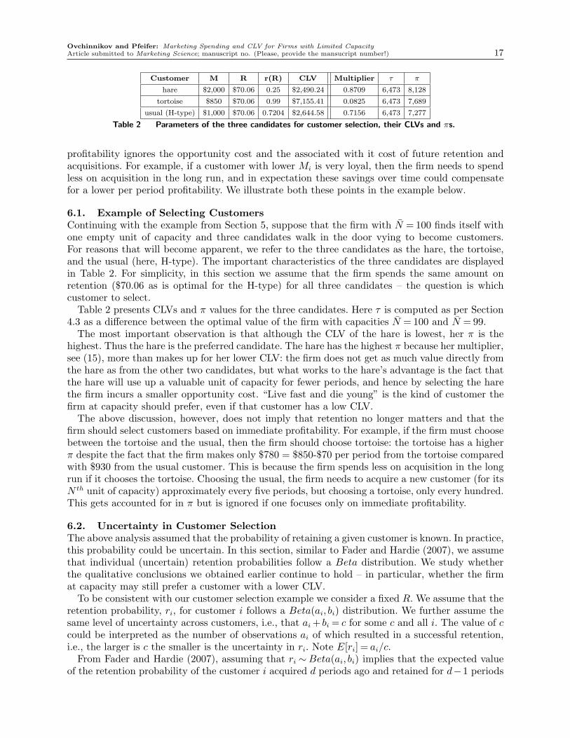
Customer M R r(R) CLV Multiplier τ π
hare $2,000 $70.06 0.25 $2,490.24 0.8709 6,473 8,128
tortoise $850 $70.06 0.99 $7,155.41 0.0825 6,473 7,689
usual (H-type) $1,000 $70.06 0.7204 $2,644.58 0.7156 6,473 7,277
Table 2 Parameters of the three candidates for customer selection, their CLVs and πs.
profitability ignores the opportunity cost and the associated with it cost of future retention andacquisitions. For example, if a customer with lower Mi is very loyal, then the firm needs to spendless on acquisition in the long run, and in expectation these savings over time could compensatefor a lower per period profitability. We illustrate both these points in the example below.
6.1. Example of Selecting CustomersContinuing with the example from Section 5, suppose that the firm with N = 100 finds itself withone empty unit of capacity and three candidates walk in the door vying to become customers.For reasons that will become apparent, we refer to the three candidates as the hare, the tortoise,and the usual (here, H-type). The important characteristics of the three candidates are displayedin Table 2. For simplicity, in this section we assume that the firm spends the same amount onretention ($70.06 as is optimal for the H-type) for all three candidates – the question is whichcustomer to select.
Table 2 presents CLVs and π values for the three candidates. Here τ is computed as per Section4.3 as a difference between the optimal value of the firm with capacities N = 100 and N = 99.
The most important observation is that although the CLV of the hare is lowest, her π is thehighest. Thus the hare is the preferred candidate. The hare has the highest π because her multiplier,see (15), more than makes up for her lower CLV: the firm does not get as much value directly fromthe hare as from the other two candidates, but what works to the hare’s advantage is the fact thatthe hare will use up a valuable unit of capacity for fewer periods, and hence by selecting the harethe firm incurs a smaller opportunity cost. “Live fast and die young” is the kind of customer thefirm at capacity should prefer, even if that customer has a low CLV.
The above discussion, however, does not imply that retention no longer matters and that thefirm should select customers based on immediate profitability. For example, if the firm must choosebetween the tortoise and the usual, then the firm should choose tortoise: the tortoise has a higherπ despite the fact that the firm makes only $780 = $850-$70 per period from the tortoise comparedwith $930 from the usual customer. This is because the firm spends less on acquisition in the longrun if it chooses the tortoise. Choosing the usual, the firm needs to acquire a new customer (for itsN th unit of capacity) approximately every five periods, but choosing a tortoise, only every hundred.This gets accounted for in π but is ignored if one focuses only on immediate profitability.
6.2. Uncertainty in Customer SelectionThe above analysis assumed that the probability of retaining a given customer is known. In practice,this probability could be uncertain. In this section, similar to Fader and Hardie (2007), we assumethat individual (uncertain) retention probabilities follow a Beta distribution. We study whetherthe qualitative conclusions we obtained earlier continue to hold – in particular, whether the firmat capacity may still prefer a customer with a lower CLV.
To be consistent with our customer selection example we consider a fixed R. We assume that theretention probability, ri, for customer i follows a Beta(ai, bi) distribution. We further assume thesame level of uncertainty across customers, i.e., that ai + bi = c for some c and all i. The value of ccould be interpreted as the number of observations ai of which resulted in a successful retention,i.e., the larger is c the smaller is the uncertainty in ri. Note E[ri] = ai/c.
From Fader and Hardie (2007), assuming that ri ∼Beta(ai, bi) implies that the expected valueof the retention probability of the customer i acquired d periods ago and retained for d−1 periods
Ovchinnikov and Pfeifer: Marketing Spending and CLV for Firms with Limited Capacity18 Article submitted to Marketing Science; manuscript no. (Please, provide the mansucript number!)
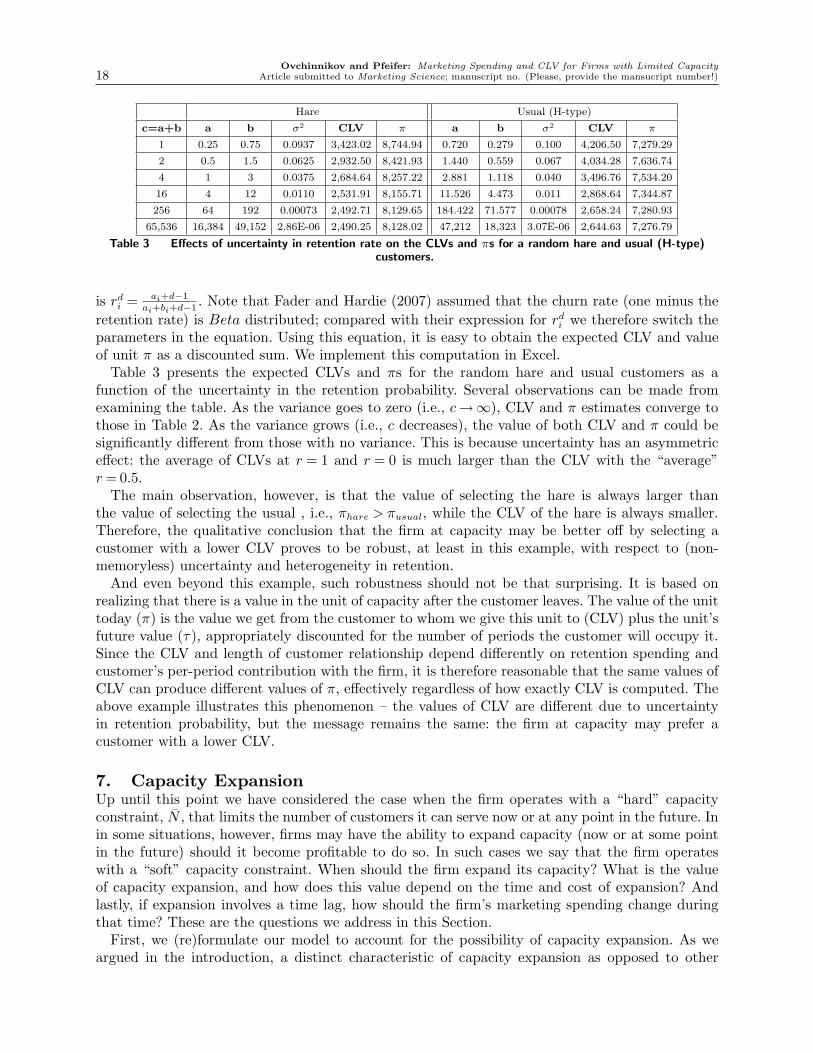
Hare Usual (H-type)
c=a+b a b σ2 CLV π a b σ2 CLV π
1 0.25 0.75 0.0937 3,423.02 8,744.94 0.720 0.279 0.100 4,206.50 7,279.29
2 0.5 1.5 0.0625 2,932.50 8,421.93 1.440 0.559 0.067 4,034.28 7,636.74
4 1 3 0.0375 2,684.64 8,257.22 2.881 1.118 0.040 3,496.76 7,534.20
16 4 12 0.0110 2,531.91 8,155.71 11.526 4.473 0.011 2,868.64 7,344.87
256 64 192 0.00073 2,492.71 8,129.65 184.422 71.577 0.00078 2,658.24 7,280.93
65,536 16,384 49,152 2.86E-06 2,490.25 8,128.02 47,212 18,323 3.07E-06 2,644.63 7,276.79
Table 3 Effects of uncertainty in retention rate on the CLVs and πs for a random hare and usual (H-type)customers.
is rdi = ai+d−1
ai+bi+d−1. Note that Fader and Hardie (2007) assumed that the churn rate (one minus the
retention rate) is Beta distributed; compared with their expression for rdi we therefore switch the
parameters in the equation. Using this equation, it is easy to obtain the expected CLV and valueof unit π as a discounted sum. We implement this computation in Excel.
Table 3 presents the expected CLVs and πs for the random hare and usual customers as afunction of the uncertainty in the retention probability. Several observations can be made fromexamining the table. As the variance goes to zero (i.e., c→∞), CLV and π estimates converge tothose in Table 2. As the variance grows (i.e., c decreases), the value of both CLV and π could besignificantly different from those with no variance. This is because uncertainty has an asymmetriceffect: the average of CLVs at r = 1 and r = 0 is much larger than the CLV with the “average”r = 0.5.
The main observation, however, is that the value of selecting the hare is always larger thanthe value of selecting the usual , i.e., πhare > πusual, while the CLV of the hare is always smaller.Therefore, the qualitative conclusion that the firm at capacity may be better off by selecting acustomer with a lower CLV proves to be robust, at least in this example, with respect to (non-memoryless) uncertainty and heterogeneity in retention.
And even beyond this example, such robustness should not be that surprising. It is based onrealizing that there is a value in the unit of capacity after the customer leaves. The value of the unittoday (π) is the value we get from the customer to whom we give this unit to (CLV) plus the unit’sfuture value (τ), appropriately discounted for the number of periods the customer will occupy it.Since the CLV and length of customer relationship depend differently on retention spending andcustomer’s per-period contribution with the firm, it is therefore reasonable that the same values ofCLV can produce different values of π, effectively regardless of how exactly CLV is computed. Theabove example illustrates this phenomenon – the values of CLV are different due to uncertaintyin retention probability, but the message remains the same: the firm at capacity may prefer acustomer with a lower CLV.
7. Capacity ExpansionUp until this point we have considered the case when the firm operates with a “hard” capacityconstraint, N , that limits the number of customers it can serve now or at any point in the future. Inin some situations, however, firms may have the ability to expand capacity (now or at some pointin the future) should it become profitable to do so. In such cases we say that the firm operateswith a “soft” capacity constraint. When should the firm expand its capacity? What is the valueof capacity expansion, and how does this value depend on the time and cost of expansion? Andlastly, if expansion involves a time lag, how should the firm’s marketing spending change duringthat time? These are the questions we address in this Section.
First, we (re)formulate our model to account for the possibility of capacity expansion. As weargued in the introduction, a distinct characteristic of capacity expansion as opposed to other

Ovchinnikov and Pfeifer: Marketing Spending and CLV for Firms with Limited CapacityArticle submitted to Marketing Science; manuscript no. (Please, provide the mansucript number!) 19
forms of limited resources (such as a budget constraint), is that expansion is “lumpy” (discreteand discontinuous): it involves some upfront onetime fixed (installation, acquisition, etc.) cost,cE, and adds some rather significant extra capacity E possibly with some time lag ∆ ≥ 1. Suchexpansions are also typically “one-off” opportunities; e.g., it is hard to imagine that the doctor’soffice will move every few years to expand capacity by, say 10 units; a far more realistic scenariois that it will move once and expand by, say 50, even if some of this newly added capacity willnot be immediately utilized. Thus we consider only a single possible expansion, which requires thefollowing modification to our model.
Observe that after the capacity is expanded, the firm’s profit-to-go is given by the functionπt(Nt, St, N + E) as defined in (6), i.e., the function is not changed, just the capacity parameterchanges. Before capacity is expanded, however, the firm’s profit-to-go function will be differentbecause it must incorporate the option of future expansion.
Let πEt (Nt, St, N) denote the firm’s profit-to-go in the case with an option to expand, and let
tE denote the time period when the firm expands (a decision variable, in addition to the decisionvector for spending, St ). Then by the above logic:
πEt (Nt, St, N) = gt(Nt, St)− cE × 1t=tE
+ β
{∫π∗t+1(w, N +E)dF(Nt,St,N+E)(w), if t≥ tE +∆− 1;∫π∗Et+1(w, N)dF(Nt,St,N)(w), if t < tE +∆− 1. (16)
where as before π∗Et+1(w, N) = maxSt+1πE
t+1(w, St+1, N) is the optimal profit-to-go.By the same argument as in the proof of Proposition 1, the difference between the optimal
profit-to-go after capacity is expanded and before is supermodular in (N , S), while for each of thetwo cases the optimal spending is decreasing in Nt. Therefore the difference, to which we refer asthe value of expanding capacity, is increasing in Nt and as a result:
Proposition 6. The optimal capacity expansion policy is of the threshold form; that is, thereexists a set of state vectors {NE} such that tE is the first period in which Nt ≥ N ∈ {NE}.And an immediate corollary to the increasing difference is that:
Corollary 2. The value of expanding capacity increases in the state Nt, and hence also in thefirm size, |Nt|.
Since the above results and formulation are stated for the general model, they also hold for thesimplified models as well. Specifically, the threshold policy takes the following form: for any NH
t
there exists a threshold function, NLE(NHt ), such that the firm should expand its capacity as soon
as it finds itself in the state (NHt ,NL
t ) with NLt ≥NLE(NH
t ). Such a threshold function, however,may be managerially difficult to work with.
A heuristic approach could be to decide on the expansion based on the total number of customers,Nt = NH
t +NLt , i.e., on the norm of the state vector rather than the vector itself. This is certainly
more managerially relevant: the firm expands as soon as its number of customers hits some NE.In our simulations we saw that the optimal (expected) profit-to-go using this heuristic was within1.5% of the optimum, starting from states in which the initial numbers of H- and L-type customerswere unbalanced by a factor of up to four. This is because the firm is continuously and activelyoptimizing its customer mix and hence seeing grossly unbalanced customer mix is unlikely; that is,the retention and acquisition spending is selected such that the ratio of H- and L-types is as closeto optimum as possible, thus deciding based on Nt is nearly optimal.
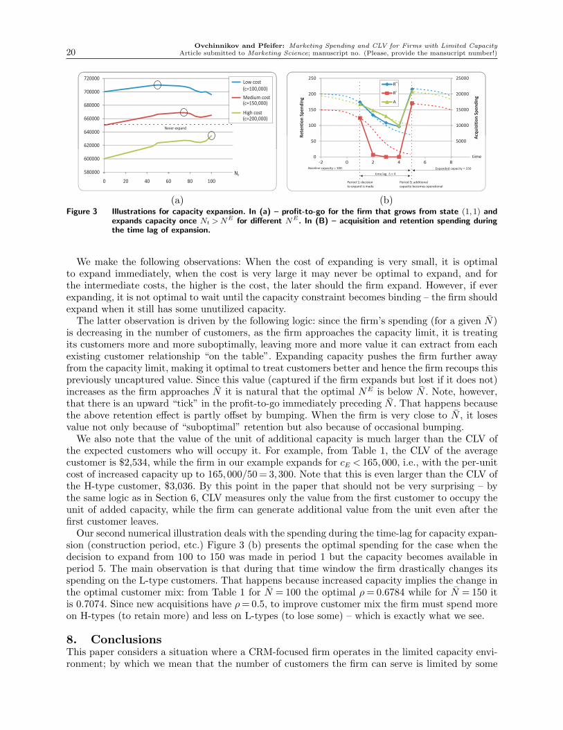
Next we use this heuristic to illustrate our results numerically based on the same parameters asin the previous sections with baseline capacity of 100 that can be expanded by 50 units. Figure 3(a) shows how the profit-to-go of the firm that follows the above heuristic depends upon the valueof NE for three costs, cE.
Ovchinnikov and Pfeifer: Marketing Spending and CLV for Firms with Limited Capacity20 Article submitted to Marketing Science; manuscript no. (Please, provide the mansucript number!)
620000
640000
660000
680000
700000
720000
580000
600000
0 20 40 60 80 100
Never expand
NE
Low cost
Medium cost
High cost
(c=100,000)
(c=150,000)
(c=200,000)
(a)
10000
15000
20000
25000
100
150
200
250
Sp
en
din
g
Re
ten
tio
nS
pe
nd
ing
5000
0
50
‐2 0 2 4 6 8
Acq
uis
itio
n
RH
A
RH
RL
time
Baseline capacity = 100 Expanded capacity = 150
Period 1, decision
to expand is made
Period 5, additional
capacity becomes operational
time lag = 4D
(b)Figure 3 Illustrations for capacity expansion. In (a) – profit-to-go for the firm that grows from state (1,1) and
expands capacity once Nt > NE for different NE. In (B) – acquisition and retention spending duringthe time lag of expansion.
We make the following observations: When the cost of expanding is very small, it is optimalto expand immediately, when the cost is very large it may never be optimal to expand, and forthe intermediate costs, the higher is the cost, the later should the firm expand. However, if everexpanding, it is not optimal to wait until the capacity constraint becomes binding – the firm shouldexpand when it still has some unutilized capacity.
The latter observation is driven by the following logic: since the firm’s spending (for a given N)is decreasing in the number of customers, as the firm approaches the capacity limit, it is treatingits customers more and more suboptimally, leaving more and more value it can extract from eachexisting customer relationship “on the table”. Expanding capacity pushes the firm further awayfrom the capacity limit, making it optimal to treat customers better and hence the firm recoups thispreviously uncaptured value. Since this value (captured if the firm expands but lost if it does not)increases as the firm approaches N it is natural that the optimal NE is below N . Note, however,that there is an upward “tick” in the profit-to-go immediately preceding N . That happens becausethe above retention effect is partly offset by bumping. When the firm is very close to N , it losesvalue not only because of “suboptimal” retention but also because of occasional bumping.
We also note that the value of the unit of additional capacity is much larger than the CLV ofthe expected customers who will occupy it. For example, from Table 1, the CLV of the averagecustomer is $2,534, while the firm in our example expands for cE < 165,000, i.e., with the per-unitcost of increased capacity up to 165,000/50 = 3,300. Note that this is even larger than the CLV ofthe H-type customer, $3,036. By this point in the paper that should not be very surprising – bythe same logic as in Section 6, CLV measures only the value from the first customer to occupy theunit of added capacity, while the firm can generate additional value from the unit even after thefirst customer leaves.
Our second numerical illustration deals with the spending during the time-lag for capacity expan-sion (construction period, etc.) Figure 3 (b) presents the optimal spending for the case when thedecision to expand from 100 to 150 was made in period 1 but the capacity becomes available inperiod 5. The main observation is that during that time window the firm drastically changes itsspending on the L-type customers. That happens because increased capacity implies the change inthe optimal customer mix: from Table 1 for N = 100 the optimal ρ = 0.6784 while for N = 150 itis 0.7074. Since new acquisitions have ρ = 0.5, to improve customer mix the firm must spend moreon H-types (to retain more) and less on L-types (to lose some) – which is exactly what we see.
8. ConclusionsThis paper considers a situation where a CRM-focused firm operates in the limited capacity envi-ronment; by which we mean that the number of customers the firm can serve is limited by some

Ovchinnikov and Pfeifer: Marketing Spending and CLV for Firms with Limited CapacityArticle submitted to Marketing Science; manuscript no. (Please, provide the mansucript number!) 21
N . The firm dynamically decides on customer-specific retention spending and on the per-periodacquisition spending in order to maximize its total net present value from sales to heterogenous cus-tomers over an infinite time horizon. To isolate the effects of the capacity constraint, we assume thatcustomer relationships are otherwise independent. That is, were it not for the capacity constraint,the firm’s optimal spending would be selected so that to separately maximize each customer’s life-time value. We seek to understand how optimal spending given the capacity constraint comparesto the CLV maximizing amounts.
We find that the optimal spending for the firm with limited capacity increases in capacity anddecreases in firm size, which contrasts to the constant (across time, number of customers, customermix, etc.) spending that is optimal for the firm with unlimited capacity. Counterintuitively, however,the optimal retention spending for the firm with limited capacity can exceed the CLV-maximizingspending. As we discuss, that happens because of the complex relationship between acquisitionand retention spending, which makes it beneficial for the firm with limited capacity to overspendon some customers and decrease the lifetime value of each relationship in order to improve thecustomer mix and save on the acquisition spending. We show that this effect is particularly strongin the cases with small discount factor; in those cases the present value of the lifetime value lossesis small, and hence the immediate savings play a bigger role.
At the same time, when the discount factor is high and the firm has only a few customers, itsoptimal spending is effectively equal to the CLV-maximizing amounts. That is, if the firm with highdiscount factor and ample unutilized capacity ignores, by mistake or on purpose, its capacity limitand spends so as to separately maximize the CLVs of its individual customers, then it operatesnearly optimal. As the firm grows, however, it should decrease its spending. Numerically we seethat the spending decreases significantly, but cetainly not all the way to zero, as some managersseem to think.
Once the firm reaches its capacity limit, it can further increase its value by optimizing thecustomer mix, and as a result converge to the case of the firm optimally at capacity. We considerthis case and provide implicit functional equations for the optimal spending. In particular, we showthat a non-discounted CLV (i.e., computed without accounting for the time value of money) ishelpful in determining the optimal spending for firm at capacity: the firm should select spendingsuch that to balance the deviations from the non-discounted CLV-maximizing spending of differentcustomers.
We also discuss customer selection. We show that selecting customers based on their CLVs ismisleading. In addition to customer CLV the firm should also consider the opportunity cost oftying-up a unit of capacity. That cost is not proportional to CLV, and as a result, the firm maybe better off by selecting a customer with a lower CLV. Likewise, the firm may be better off byselecting a customer that contributes less to the firm each period. We also show that these findingsare robust with respect to the uncertainty in retention probability.
Lastly, we extended our model to the case when the firm can expand its limited capacity. Adistinct characteristic of limited capacity, as opposed to other forms of limited resources (such asfor example a budget constraint), is that expansion is “lumpy” and discontinuous: it involves asignificant upfront fixed cost, which adds a significant number of units of capacity, possibly witha delay. We show that the optimal expansion policy is of the threshold form. At optimality thedecision involves a vector of customer counts, but a simple managerial heuristic is to expand whenthe total number of customers becomes large enough. We show that it is not optimal to wait withexpansion until capacity becomes binding: the firm should expand even in anticipation of capacitylimit because it allows for extracting more value out of each customer relationship. Decision forwhen to expand is naturally related to cost: the larger is the cost, the later should the firm expand;in any case, the value of added unit of capacity is much larger than the CLV of the customerwho will occupy it. Finally, if expansion involves the time lag, then the firm’s spending changes
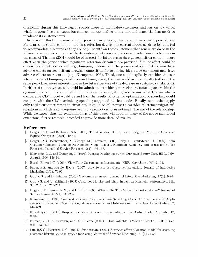
Ovchinnikov and Pfeifer: Marketing Spending and CLV for Firms with Limited Capacity22 Article submitted to Marketing Science; manuscript no. (Please, provide the mansucript number!)
drastically during this time lag: it spends more on high-value customers and less on low-value,which happens because expansion changes the optimal customer mix and hence the firm needs torebalance its customer mix.
In terms of the future research and potential extensions, this paper offers several possibilities.First, price discounts could be used as a retention device; our current model needs to be adjustedto accommodate discounts as they are only “spent” on those customers that renew; we do so in thefollow-up paper. Second, a possible dependency between acquisition and retention effectiveness inthe sense of Thomas (2001) could be of interest for future research; e.g., acquisition could be moreeffective in the periods when significant retention discounts are provided. Similar effect could bedriven by competition as well: e.g., bumping customers in the presence of a competitor may haveadverse effects on acquisition; likewise competition for acquiring high-value customers may haveadverse effects on retention (e.g., Klemperer 1995). Third, one could explicitly consider the casewhere instead of bumping a customer and losing a sale, the firm would incur a penalty (either in thesame period, or, more interestingly, in the future because of the decrease in customer satisfaction).In either of the above cases, it could be valuable to consider a more elaborate state space within thedynamic programming formulation; in that case, however, it may not be immediately clear what acomparable CLV model would be and how the results of dynamic optimization of spending wouldcompare with the CLV-maximizing spending suggested by that model. Finally, our models applyonly to the customer retention situations; it could be of interest to consider “customer migration”situations in which a non-response (e.g., to a promotion) does not imply the end of the relationship.While we expect that the general findings of this paper will apply in many of the above mentionedextensions, future research is needed to provide more detailed results.
References[1] Berger, P.D., and Bechwati, N.N. (2001). The Allocation of Promotion Budget to Maximize Customer
Equity, Omega 29 (2001), 49-61.
[2] Berger, P.D., Eechambadi, N., George, M., Lehmann, D.R., Rizley, R., Venkatesan, R. (2006). FromCustomer Lifetime Value to Shareholder Value: Theory, Empirical Evidence, and Issues for FutureResearch. Journal of Service Research, 9(2), 156-167.
[3] Blattberg, R.C. and Deighton, J. (1996). Manage Marketing by the Customer Equity Test, HBR, July-August 1996, 136-144.
[4] Bursk, Edward C. (1966), View Your Customers as Investments, HBR, May/June 1966, 91-94.
[5] Fader, P.S. and Hardie, B.G.S. (2007). How to Project Customer Retention, Journal of InteractiveMarketing 21(1), 76-90.
[6] Gupta, S. and D. Lehman. (2003) Customers as Assets. Journal of Interactive Marketing, 17(1), 9-24.
[7] Gupta S. and V. Zeithaml (2006) Customer Metrics and Their Impact on Financial Performance. MktSci 25(6) pp. 718-739
[8] Hogan, J.E., Lemon, K.N., and B. Libai (2003) What is the True Value of a Lost customer? Journal ofService Research, 5(3), 196-208.
[9] Klemperer P. (1995) Competition when Consumers have Switching Costs: An Overview with Appli-catoins to Industrial Organization, Macroeconomics, and International Trade. Rev Econ Studies, 62,515-539.
[10] Kowalczyk, L. (2006) Hospital doctors shut doors to new patients. The Boston Globe. November 12,2006.
[11] Kumar, V., J. A. Petersen, and R. P. Leone (2007). ”How Valuable is Word of Mouth?”, HBR, Oct.2007, 139-146.
[12] Liu, B.S-C., Petruzzi, N.C., and D. Sudharshan. (2007) A service effort allocation model for assessingcustomer lifetime value in service marketing. Journal of Services Marketing. 21 (1) 24-35

Ovchinnikov and Pfeifer: Marketing Spending and CLV for Firms with Limited CapacityArticle submitted to Marketing Science; manuscript no. (Please, provide the mansucript number!) 23
[13] Lewis M., 2005. Research Note: A Dynamic Programming Approach to Customer Relationship Pricing.ManSci Vol. 51 (6) pp. 986-994.
[14] Pfeifer, P.E., (1999). On the Use of Customer Lifetime Value as a Limit on Acquisition Spending,Journal of Database Marketing, 7(1), 81-86.
[15] Pfeifer, P.E. and A. Ovchinnikov (2010) Customer Lifetime Value for Firms with Limited Capacity.Working paper, University of Virginia.
[16] Roemer, Ellen (2006). The Impact of Dependence on the Assessment of Customer Lifetime Value inBuyer-Seller Relationships, Journal of Marketing Management, 22, 89-109.
[17] Rust R. T. and T.S. Chung (2006) Marketing Models of Service and Relationships. Mkt Sci 25(6) pp.560-580
[18] Rust, R.T., Zeithaml, V.A., and Lemon, K.N., (2000). Driving Customer Equity: How Customer LifetimeValue is Reshaping Corporate Strategy, The Free Press, New York, NY, USA
[19] Sun B. (2006) Technology Innovation and Implications for Customer Relationship Management. MktSci 25(6) pp. 594-597
[20] Thomas J. S. (2001). A methodology for Linking Customer Acquisition to Customer Retention. JMR38(), 262-268
[21] Topkis, D. M. 1998. Supermodularity and Complimentarity. Princeton U. Press. New Jersey.
[22] Wiesel, T., Skiera, B., and Villanueva, J. (2008). Customer Equity: An Integral Part of FinancialReporting, Journal of Marketing, Vol. 72 (March, 2008), 1-14.

Ovchinnikov and Pfeifer: Marketing Spending and CLV for Firms with Limited Capacity24 Article submitted to Marketing Science; manuscript no. (Please, provide the mansucript number!)
Appendix. ProofsProof of Proposition 1. Recall that if a distribution Jx(y) is stochastically increasing (concave, supermodular,etc.) in parameter x, then the expectation of any increasing function j(y),
∫j(y)dJx(y), is also increasing
(concave, supermodular, etc.) in x (e.g., see Topkis 1998, proposition 3.9.1).Further, because Nt and St are vectors, with respect to the above result, “increasing” means that at least
one component of the vector in increasing, while other components do not decrease (see Topkis 1998, Section2.2). Consider arbitrary components Nt and St that we will increase, and assume other components do notchange (this can be done without loss of generality, because an increase in multiple components can berepresented as a series of single-component-only increases). From the above result, because g is increasingin Nt and N and F is stochastically increasing in Nt and N , by induction π∗t+1 is increasing in Nt and N .Thus,
∂2π
∂N∂St
= β
∫∂π∗t+1
∂N
∂
∂St
dF + β
∫π∗t+1
∂2
∂N∂St
dF ≥ 0
because, in addition to the increasing properties established above, in the first term F is stochasticallyincreasing in St, and in the second term F is stochastically supermodular in (N ,St). Since components Nt
and St were selected arbitrary, πt(Nt, St, N) is supermodular in (N , St) and therefore the optimal spendingS∗t (N) is increasing in N . Q.E.D.Proof of Proposition 2. Let D(N,ρ,S) to be the maximum demand that the firm with N customers withaggregate quality ρ today can face next period if it spends S in total:
D(N,ρ,S) = maxA,RH ,RL, such that NρRH+N(1−ρ)RL+A=S
[NρrH(RH)+ N(1− ρ)rL(RL)+n(A)]. (17)
Observe that if D(·) is increasing, then min[N ,D(·)] is supermodular in (N , ·). Lemma 1 establishes theincreasing and some useful properties of D(·) which we then use to prove the proposition.
Lemma 1. Let R∗H(N,ρ,S), R∗L(N,ρ,S) and A∗(N,ρ,S) be the solutions to the demand function opti-mization problem (17). Then:(a) R∗H(N,ρ,S), R∗L(N,ρ,S) and A∗(N,ρ,S) exist and are unique;
(b) R∗H(N,ρ,S), R∗L(N,ρ,S) and A∗(N,ρ,S) increase in S and decrease in N and ρ;
(c) R∗H(N,ρ,S)≥R∗L(N,ρ,S);
(d) D(N,ρ,S) is increasing in N , ρ and S.
Proof of Lemma 1. Part (a). Because n(·), rL(·) and rH(·) are concave, NρrH(RH)+N(1−ρ)rL(RL)+n(A)is also concave. Therefore the optimal A∗, R∗L and R∗H satisfy Lagrangian FOC:
{NρRH +N(1− ρ)RL + A = S∂n∂A
= ∂rL
∂RL = ∂rH
∂RH =−λ.
Since n(·), rL(·) and rH(·) are increasing and concave, the optimal A∗(λ), RL(λ) and RH(λ) exist andare unique. Further, it is easy to see that all three optimal decisions are increasing in λ (note that λ≤ 0).Therefore, the optimal λ∗(N,ρ,S) also exists and is unique, and so A∗(N,ρ,S), RL(N,ρ,S) and RH(N,ρ,S)exist and are unique.
Part (b). The result follows by implicit differentiation of the constraint for D (first equation in the FOCabove) at the optimal A∗(λ∗(N,ρ,S)), RL(λ∗(N,ρ,S)) and RH(λ∗(N,ρ,S)). The cases with N and S arestraightforward. For the case of ρ, ∂λ∗/∂ρ satisfies:
N(R∗H −R∗L
)+
∂λ∗
∂ρ
(∂A∗
∂λ+ N
(ρ∂R∗H
∂λ+(1− ρ)
∂R∗L
∂λ
))= 0
and so∂λ∗
∂ρ=− N (R∗H −R∗L)
∂A∗∂λ
+ N(ρ ∂R∗H
∂λ+(1− ρ) ∂R∗L
∂λ
) ≤ 0 (18)
if R∗H ≥R∗L, which we show next.Part (c). By assumption rL(·) and rH(·) are increasing concave and at each point the slope of rH is higher
than the slope of rL. Since at the optimal R∗H and R∗L, the slopes of rH and rL are equal (to −λ), ittherefore follows that R∗H ≥R∗L.

Ovchinnikov and Pfeifer: Marketing Spending and CLV for Firms with Limited CapacityArticle submitted to Marketing Science; manuscript no. (Please, provide the mansucript number!) 25
Part (d). We show only the proof for the property in ρ; properties in N and S can be established similarly.By differentiating D over ρ at A∗(λ∗(N,ρ,S)), RL(λ∗(N,ρ,S)) and RH(λ∗(N,ρ,S)) we obtain:
∂D
∂ρ= N
(rH(R∗H
)− rL(R∗L))+∂A∗
∂λ
∂λ∗
∂ρ
∂n
∂A+ N
(ρ∂R∗H
∂λ
∂λ∗
∂ρ
∂rH
∂RH+(1− ρ)
∂R∗L
∂λ
∂λ∗
∂ρ
∂rL
∂RL
)
= N(rH(R∗H)− rL(R∗L)
)−λ∗∂λ∗
∂ρ
(∂A∗
∂λ+ N
(ρ∂R∗H
∂λ+(1− ρ)
∂R∗L
∂λ
))
= N(rH(R∗H)− rL(R∗L)+ λ∗(R∗H −R∗L)
)≥ 0
where the first equation holds because at the optimum ∂n∂A
= ∂rL
∂RL = ∂rH
∂RH =−λ, the second follows from (18),and the inequality follows from (c) because rL and rH are concave, rH has a steeper slope and because atoptimum slopes are equal to −λ. Q.E.D.Proof of Proposition 2 continued. Since by the assumption ∂rH/∂x≥ ∂rL/∂x, and ρ, ξ ≤ 1, it is not difficultto verify that Nt+1 and ρt+1 are increasing in (Nt, ρt, St). Further, for all RH ,RL,A such that NtρtR
H +Nt(1 − ρt)RL + A = St for any given St, gt is increasing in Nt and ρt. Combining these results with (d)of the Lemma, the simplified model satisfies the assumptions of the general model discussed in Section3.2 with decision St and state space Nt = NH + NL. That is, the total optimal marketing spending S∗t ≡NtρtR
∗Ht + Nt(1− ρt)R∗L
t + A∗t is increasing in the firm’s capacity, N and is decreasing in firm’s size Nt.
From (b) both acquisition and retention components of spending also increase with N and decrease with Nt.Further, from (c) at all times the firm spends more on retaining high-value customers. Q.E.D.