Market Structure and the Behavior

of Firms

Perfect Competition vs Monopoly

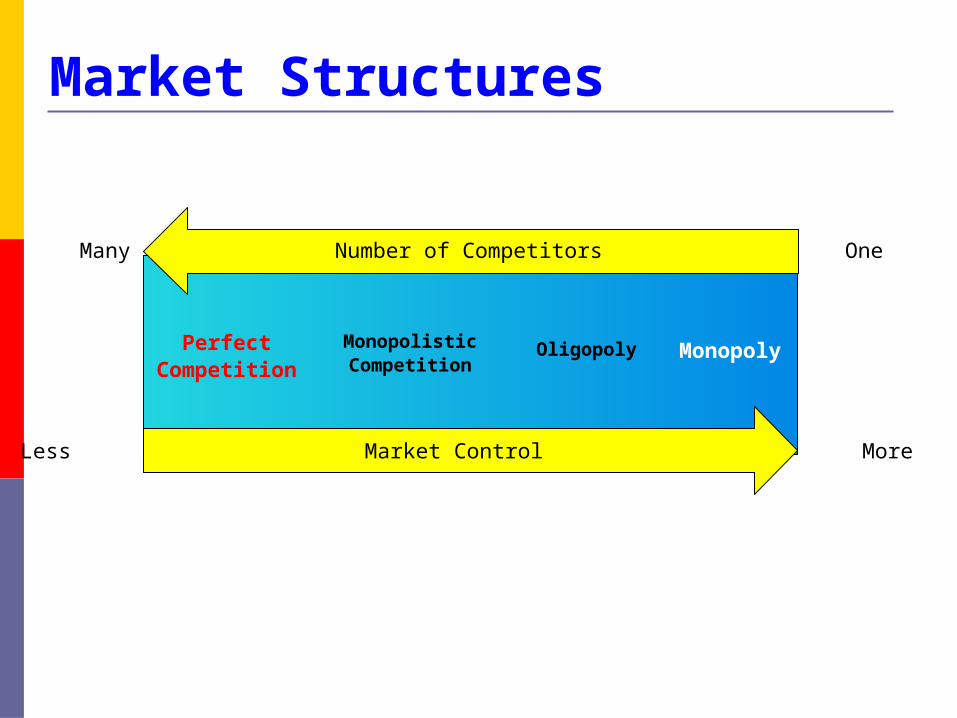
Market Structures

Many Number of Competitors One

Less Market Control More

PerfectCompetition

MonopolyMonopolisticCompetition

Oligopoly

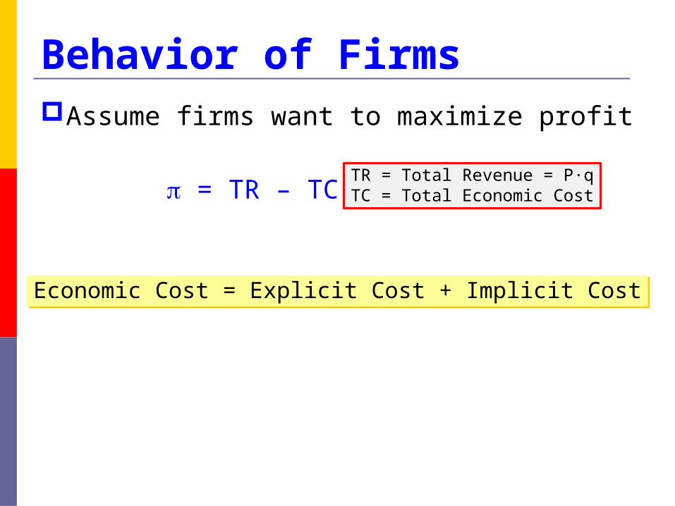
Assume firms want to maximize profit

= TR – TC

Behavior of Firms

TR = Total Revenue = P∙qTC = Total Economic Cost

Economic Cost = Explicit Cost + Implicit CostEconomic Cost = Explicit Cost + Implicit Cost

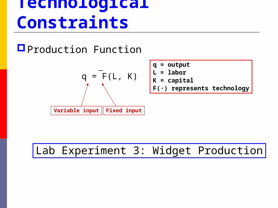
Technological ConstraintsProduction Function

q = F(L, K)

q = outputL = laborK = capitalF(·) represents technology

Lab Experiment 3: Widget Production

_

Variable input Fixed input

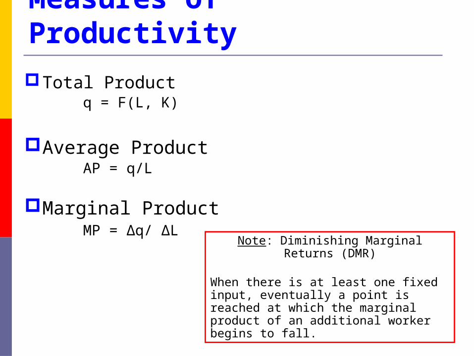
Measures of Productivity

Total Product q = F(L, K)

Average Product AP = q/L

Marginal Product MP = Δq/ ΔL

Note: Diminishing Marginal Returns (DMR)

When there is at least one fixed input, eventually a point is reached at which the marginal product of an additional worker begins to fall.

∆q

∆L

Productivity Graphs

labor

output

labor

q/L

TP

MP

AP

L1L1

DMR

L2

L2

Slope = MPL = ∆q/ ∆L

When MP > AP then AP will riseWhen MP < AP then AP will fall

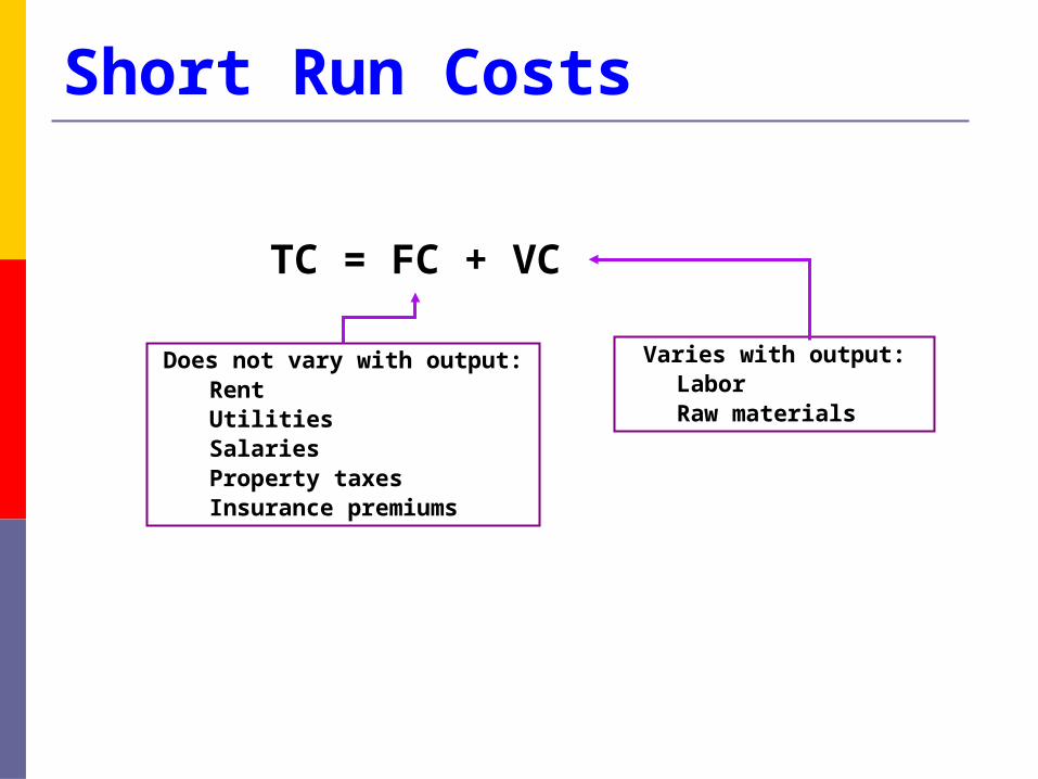
Short Run Costs

TC = FC + VC

Does not vary with output:RentUtilitiesSalariesProperty taxesInsurance premiums

Varies with output:Labor Raw materials

Short Run Cost Curve Family

output

$

output

$

FC

VC

TC

AFC

MC

AVC

ATC

TC = FC + VC ATC = AFC + AVC

ΔTCMC=

Δq

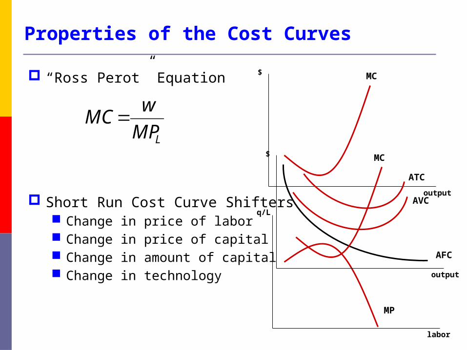
Properties of the Cost Curves

“Ross Perot” Equation

Short Run Cost Curve Shifters Change in price of labor Change in price of capital Change in amount of capital Change in technology

LMP

wMC

output

$ MC

labor

q/L

MP

output

$

AFC

MC

AVC

ATC

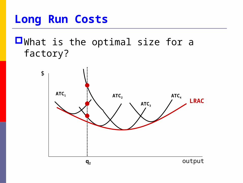
Long Run Costs

What is the optimal size for a factory?

output

$

ATC1 ATC2

ATC3

ATC4

q2

LRAC

Long Run Average Cost Curve

output

$

ATC3

LRAC

qMES

EOS: double the inputs, output more than doubles

DOS: double the inputs, output less than doubles

LRAC falls

LRAC rises

SpecializationSpecialization Coordination/Communication Problems

Coordination/Communication Problems

Perfect Competition: Price Taker Model

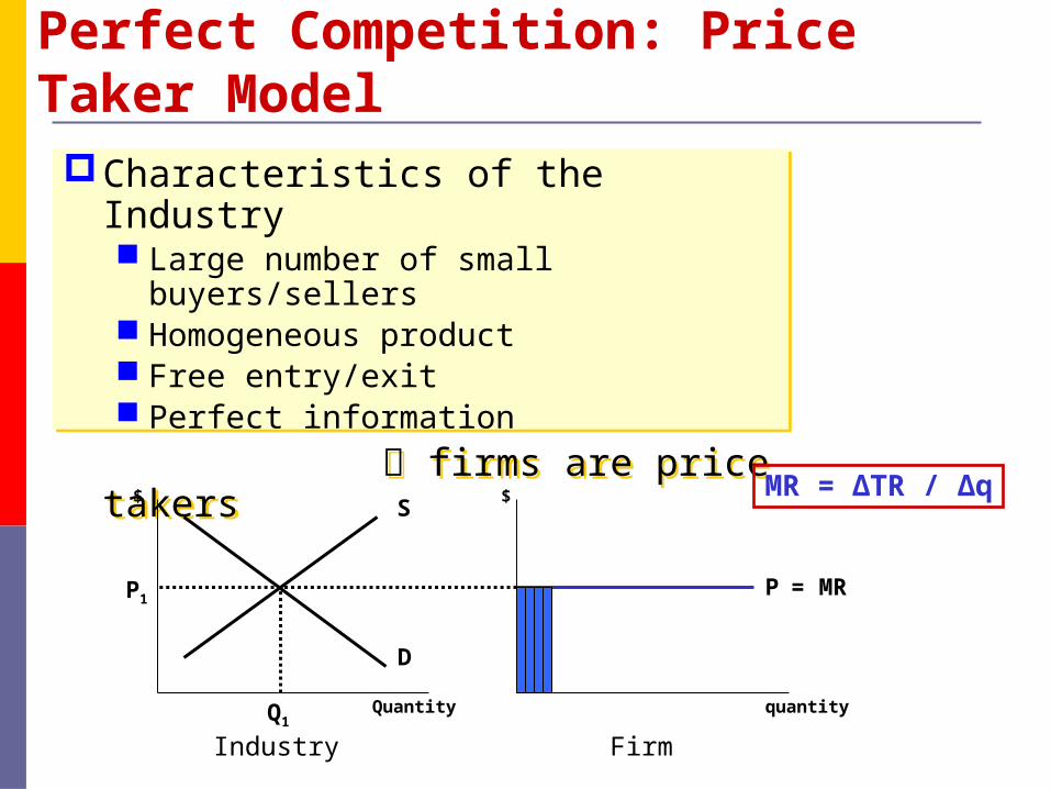
Characteristics of the Industry Large number of small buyers/sellers Homogeneous product Free entry/exit Perfect information

firms are price takers

Characteristics of the Industry Large number of small buyers/sellers Homogeneous product Free entry/exit Perfect information

firms are price takers

S

D

PP1

Q1Quantity quantity

$

Industry Firm

= MR

MR = ΔTR / Δq$

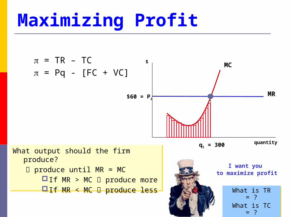
Maximizing Profit

= TR – TC = Pq - [FC + VC]

What output should the firm produce? produce until MR = MC

If MR > MC produce moreIf MR < MC produce less

What output should the firm produce? produce until MR = MC

If MR > MC produce moreIf MR < MC produce less

MR

MC

quantity

$

q1 = 300

$60 = P1

I want you to maximize profit

What is TR = ?What is TC = ?What is TR = ?What is TC = ?

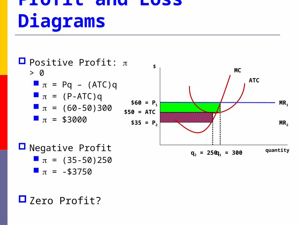
Profit and Loss Diagrams

MC

quantity

$

q1 = 300

$60 = P1

ATC

MR1

$50 = ATC

Positive Profit: > 0 = Pq – (ATC)q = (P-ATC)q = (60-50)300 = $3000

Negative Profit = (35-50)250 = -$3750

Zero Profit?

MR2$35 = P2

q2 = 250

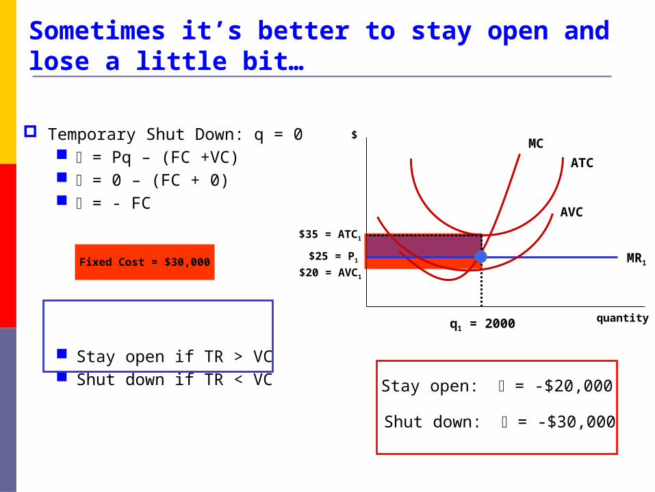
Sometimes it’s better to stay open and lose a little bit…

Temporary Shut Down: q = 0 = Pq – (FC +VC) = 0 – (FC + 0) = - FC

Stay open if TR > VC Shut down if TR < VC

MC

quantity

$

q1 = 2000

$25 = P1

ATC

MR1

$35 = ATC1

AVC

$20 = AVC1

Stay open: = -$20,000

Shut down: = -$30,000

Fixed Cost = $30,000

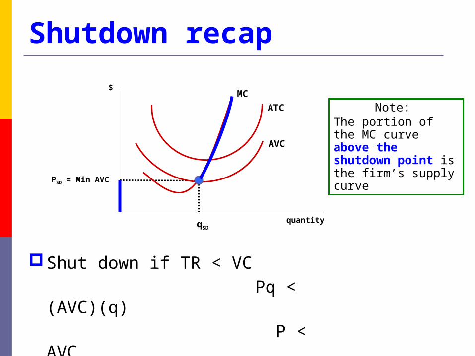
Shutdown recap

Shut down if TR < VC Pq < (AVC)(q) P < AVC

MC

quantity

$

qSD

ATC

AVC

PSD = Min AVC

Note: The portion of the MC curve above the shutdown point is the firm’s supply curve

How should a business react if…

Price rises?Marginal costs rise?Fixed costs rise?

MC

quantity

$

q1

P1

ATC

MR1

AVC

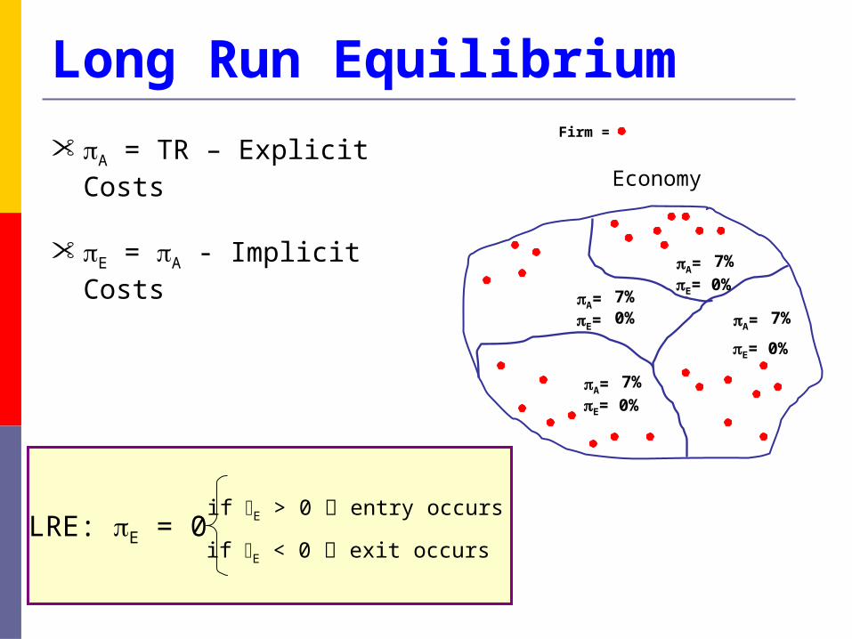
Long Run Equilibrium

• A = TR – Explicit Costs

• E = A - Implicit Costs

A= 6%

A= 6%

A= 6%A= 9%E= 3%

if E > 0 entry occurs

if E < 0 exit occurs

Economy

E= 0%

E= 0%

E= 0%

7%

7%

7%

7%0%

Firm =

LRE: E = 0

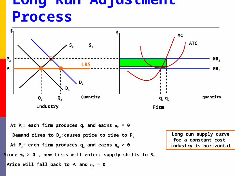
Long Run Adjustment Process

MC

quantity

$

q1

P1

ATC

MR1

MR2

D1

S1

Q1

At P1: each firm produces q1 and earns E = 0

Demand rises to D2:

D2

S2

P2

At P2: each firm produces q2 and earns E > 0

Since E > 0 , new firms will enter: supply shifts to S2

Price will fall back to P1 and E = 0

q2Q3

Industry Firm

Quantity

$

LRS

Long run supply curvefor a constant cost

industry is horizontal

causes price to rise to P2

MES and Market Structure

D

Output

$

Q1

P1

⅛Q1 ¼Q1 ½Q1

ATC1

ATC2 ATC3

ATC4

The greater MES is as a share of market demand, the fewer the number of firms

Industry 1: room for 8 firmsIndustry 2: room for 4 firms Industry 3: room for 2 firms Industry 4: room for 1 firm

“natural monopoly”

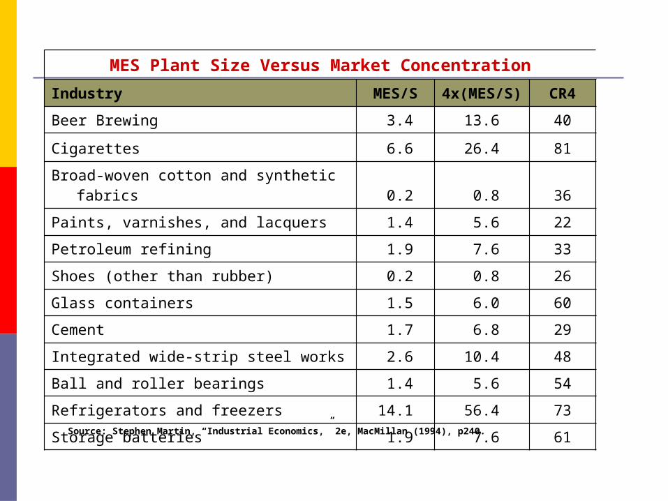
MES Plant Size Versus Market Concentration

Industry MES/S4x(MES/

S) CR4

Beer Brewing 3.4 13.6 40

Cigarettes 6.6 26.4 81

Broad-woven cotton and synthetic fabrics 0.2 0.8 36

Paints, varnishes, and lacquers 1.4 5.6 22

Petroleum refining 1.9 7.6 33

Shoes (other than rubber) 0.2 0.8 26

Glass containers 1.5 6.0 60

Cement 1.7 6.8 29

Integrated wide-strip steel works 2.6 10.4 48

Ball and roller bearings 1.4 5.6 54

Refrigerators and freezers 14.1 56.4 73

Storage batteries 1.9 7.6 61Source: Stephen Martin, “Industrial Economics,” 2e, MacMillan (1994), p240.

MonopolyA Price Searcher Model

Monopoly

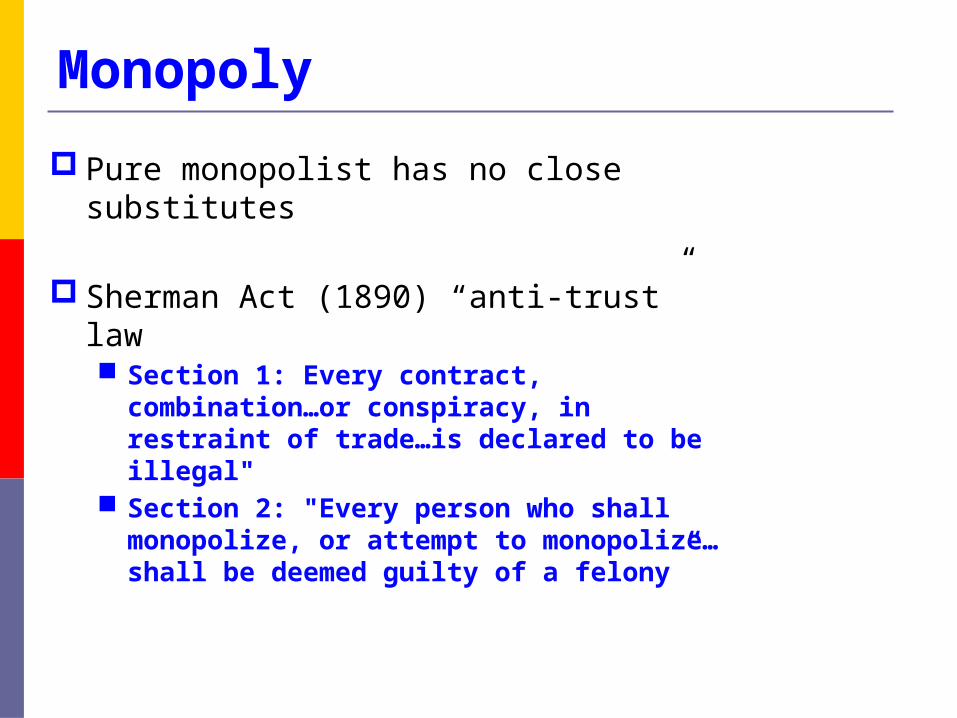
Pure monopolist has no close substitutes

Sherman Act (1890) “anti-trust” law Section 1: Every contract, combination…

or conspiracy, in restraint of trade…is declared to be illegal"

Section 2: "Every person who shall monopolize, or attempt to monopolize…shall be deemed guilty of a felony”

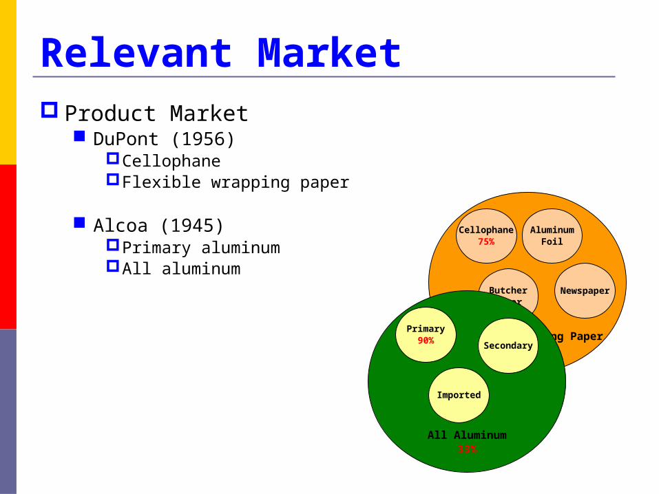
Relevant Market Product Market

DuPont (1956)CellophaneFlexible wrapping paper

Alcoa (1945)Primary aluminumAll aluminum

Flexible Wrapping Paper20%

Cellophane75%

AluminumFoil

ButcherPaper

Newspaper

All Aluminum33%

Primary90%

Secondary

Imported

Global

Relevant Market Geographic Market

Local Regional National Global

Local

Regional

National

Barriers to Entry Economies of Scale

“natural monopoly” Control over key inputs

Alcoa--bauxite DeBeers

GE Superabrasives (Diamond Innovations)

LRAC

Quantity

$

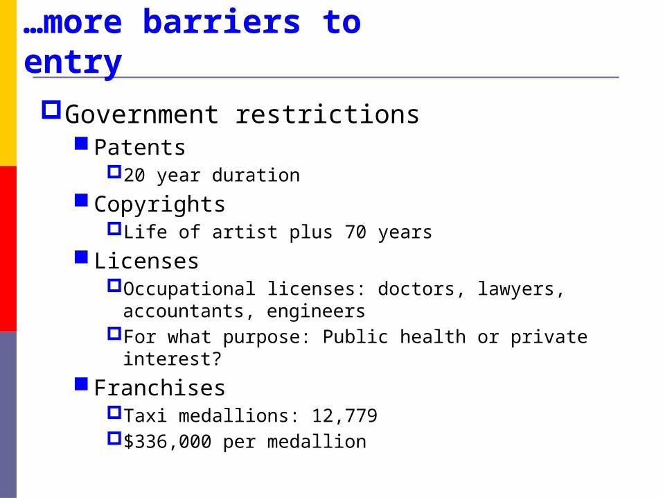
…more barriers to entryGovernment restrictions

Patents20 year duration

CopyrightsLife of artist plus 70 years

Licenses Occupational licenses: doctors, lawyers, accountants,

engineersFor what purpose: Public health or private interest?

FranchisesTaxi medallions: 12,779$336,000 per medallion

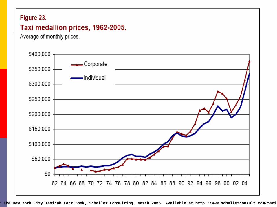
Source: The New York City Taxicab Fact Book, Schaller Consulting, March 2006. Available at http://www.schallerconsult.com/taxi/taxifb.pdf

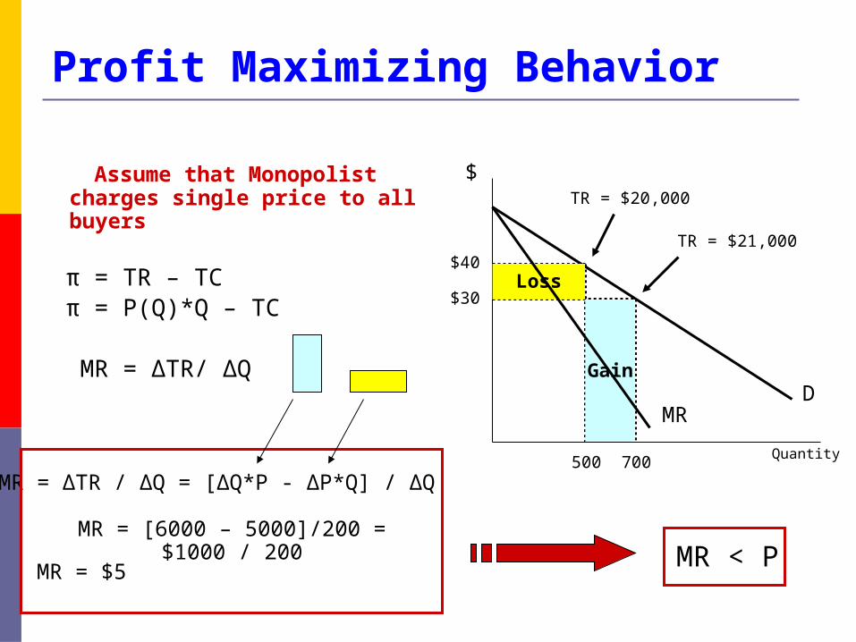
Profit Maximizing Behavior

Assume that Monopolist charges single price to all buyers

π = TR – TC π = P(Q)*Q – TC

MR = ∆TR/ ∆Q

$

$40

$30

500 700

D

TR = $20,000

TR = $21,000

MR = ∆TR / ∆Q = [∆Q*P - ∆P*Q] / ∆Q

Loss

Gain

MR = [6000 – 5000]/200 = $1000 / 200

MR = $5 MR < P

Quantity

MR

MR, P, and Elasticity

Note: If E > 1 then MR > 0 If E < 1 then MR < 0 If E = 1 then MR = 0 If E = ∞ then MR = P [Perfect Competition]

MR = P [ 1 – 1/E ]MR = P [ 1 – 1/E ]

MR = ∆TR / ∆Q = [∆Q*P - ∆P*Q] / ∆Q

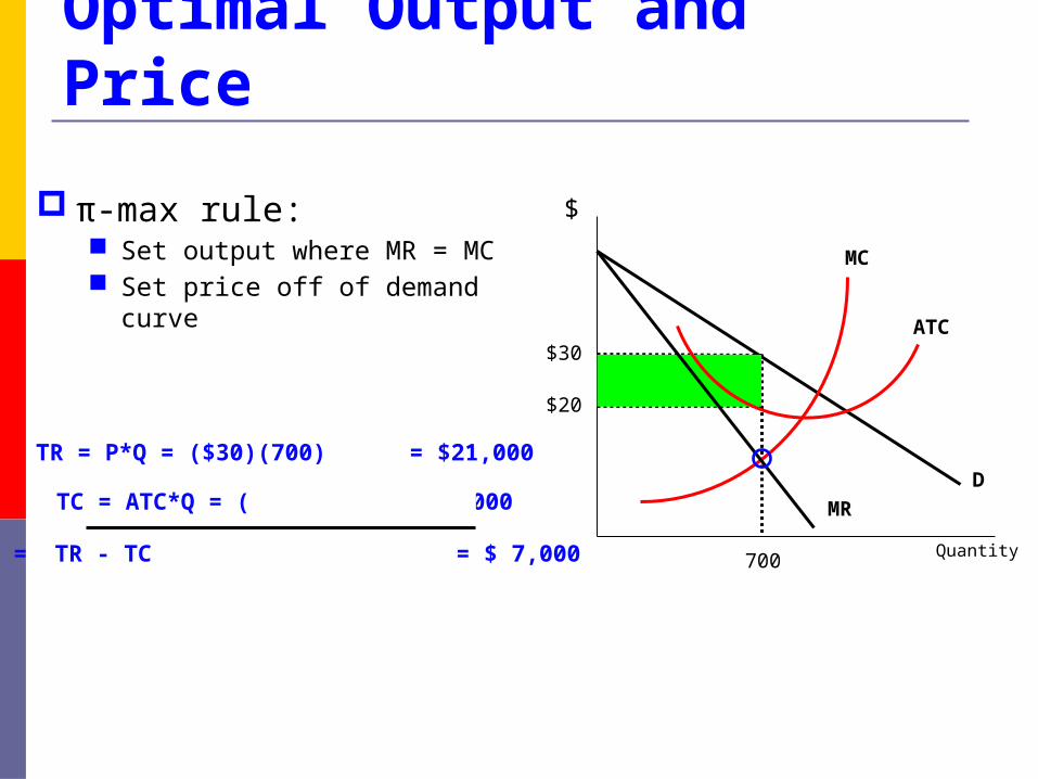
Optimal Output and Price

π-max rule: Set output where MR = MC Set price off of demand curve

$

$20

$30

700

D

Quantity

MR

MC

ATC

TR = P*Q = ($30)(700) = $21,000

TC = ATC*Q = ($20)(700) = $14,000

π = TR - TC = $ 7,000

Optimal Output and Price

π-max rule: Set output where MR = MC Set price off of demand curve

How will monopolist react to: an increase in marginal cost? an increase in fixed cost? an increase in demand?

$

$20

$30

700

D

Quantity

MR

MC

ATC

Welfare Comparison: PC vs. Monop

Perfect Competition: PC, QC

Monopoly: PM, QM

$

D

Quantity

MR

MC = ATC

QcQM

PM

PC

A

B C

PC Monop

CS

PS

Social Welfare

DWL

A+B+C

A+B+C

---

---

A

B

A+B

C

Price Discrimination Definition: price differentials that do not reflect

cost differentials Motivation: to increase profits by capturing more

consumer surplus Necessary Conditions

Market Power Downward sloping demand curve

Segment the market Demographics Usage rates

Prevent resale Movie theatres Röhm-Haas: plastic molding compound

Industrial: $0.85/lb

Dentists: $22/lb

Arsenic ?

Types of Price Discrimination

First Degree Charge each buyer their WTP Captures all CS and DWL

Second Degree Quantity discounts

Third Degree Set prices according to price

elasticity Movie Theatre

MRA = MRK = MC

$

D

Quantity

MR

QcQM

PM

PC MC

MC = $4

EA = 2

EK = 5

MRA = PA[1 – 1/EA]

MRA = MC

PA[1 – 1/2] = 4 PA = $8Charge higher price

to more inelastic group

United States v. Microsoft (2000) Operating Systems

Windows 90% Macs 8% Linux -- Java --

Application Software Word Excel Powerpoint Outlook Access Internet Explorer

“Bundling”