Market Structure and Innovation:

A Dynamic Analysis of the Global Automobile Industry∗

Aamir Rafique Hashmi†

and

Johannes Van Biesebroeck‡

August 6, 2007

Abstract

The question how market structure and innovation are related has been extensively studied

in the literature. However, no studies exist for the automobile industry, which spends more on

R&D than any other industry. We fill this gap by studying the relationship between market

structure and innovation in the global automobile industry for the 1980-2005 period. We use

the dynamic industry framework of Ericson and Pakes [1995] and estimate the parameters of

the model using a two-step procedure proposed by Bajari et al. [2007]. Since the industry has

seen a lot of consolidation since 1980, mergers are an important ingredient of our model.

After estimating the parameters of the model, we simulate the industry forward and study

how changing market structure (mainly due to mergers) affects innovative activity at the firm as

well as at the industry level. Our findings are the following: (1) The effect of market structure

on innovation in the global auto industry depends on the initial state. If the industry is not

very concentrated, as it was in 1980, some consolidation may increase the innovative activity.

However, if the industry is already concentrated, as in 2005, further consolidation may reduce

the incentives to innovate. (2) Mergers reduce the value of merging firms though they may

increase the aggregate value of the industry. (3) Mergers between big firms eventually reduce

consumers’ utility.

Key words: Competition and Innovation; Automobile Industry; Dynamic Games

JEL Classification Codes: C73; L13; L62; O31

∗We thank participants at the conferences of the CEA (Montreal and Halifax), EEA (Vienna), IIOC (Savannah),

SED (Prague), and the CEPA seminar at the University of Toronto for their comments. Financial support from

AUTO21, CFI, and SSHRC is greatly appreciated.†Departments of Economics, National University of Singapore and University of Toronto. E-mail:

aamir.hashmi@gmail.com‡Department of Economics, University of Toronto and NBER. E-mail: johannes.vanbiesebroeck@utoronto.ca

1

1 Introduction

In this paper, we investigate how changes in industry structure interact with the innovative activity

of the incumbent firms in the global automobile industry. The question of interaction between

market structure and innovation has been the subject of intense research since Schumpeter [1950].1

However, there is hardly any study on the global automobile industry. This is surprising given the

fact that the global automobile industry has not only undergone interesting changes in its market

structure in recent years, but is also one of the most innovative industries in the global economy.

The global automobile industry has seen significant consolidation over the last few decades.

Many of the industry giants have found it beneficial to join hands with some of their former rivals.

The mergers between Daimler-Benz and Chrysler and between Hyundai and Kia, the association

between Renault and Nissan and the takeover of Mazda, Jaguar and Volvo by Ford are but a

few examples of this consolidation. On the one hand, this consolidation is the result of increased

competition, which has made it harder for smaller firms to survive on their own. On the other

hand, consolidation intensifies competition as the emerging groups are highly research intensive.

The top 13 firms in the auto industry spent more than 55 billion dollars on R&D in 2005 and have

obtained more than 50,000 patents from the US patent office between 1980 and 2004.

Increasingly, producing cars is a highly research intensive activity: in 2003, more than 13% of all

R&D in the OECD was spent in ISIC industry 34 ‘Motor Vehicles’, more than in any other industry.

Statistics in Table 1 illustrate the comparative importance of R&D in the automotive industry

for the OECD and the three largest economic blocs. The industry is concentrated worldwide,

guaranteeing that the main firms will take actions of competitors into account when deciding on

their own innovative activities. In 2005, more than 85% of all vehicles were produced by the 13

largest firms, which are active in all major regions of the world.2

[Table 1 approximately here]

At the most fundamental level, two features are necessary for innovation to take place. First,

firms need to be able to finance innovation, i.e. there needs to be a margin between price and

marginal cost. Second, firms need to have an incentive to innovate, i.e. innovation has to increase

expected profits. Both conditions are clearly satisfied in the automobile industry. Demand estimates

for this industry—see for example Berry et al. [1995] or Goldberg [1995]—reveal that markups over

marginal costs tend to be large, consistent with the view that fixed costs are important in this1Kamien and Schwartz [1982], Cohen and Levin [1989], Ahn [2002] and Gilbert [2006] are surveys of the relevant

literature.2Throughout, we do not distinguish between minority share holdings and outright control. E.g. Mazda is counted

as part of the Ford group, even though Ford Motor Co. never held more than 33.4% of Mazda’s shares (achieved by

1996).

2

industry. Innovation is also likely to advance a firm’s competitive position through higher product

quality and reliability, the introduction of desirable features in its products, or lower production

cost. A large number of analysts makes a living measuring these benefits for consumers and investors

alike.3

Unlike most of the studies that use reduced form regressions to study the relationship between

market structure and innovation, we do so in a strategic and dynamic environment. There are at

least two reasons for this. First, innovation is inherently a dynamic activity. Firms make R&D

investments today expecting uncertain future rewards through better products or more efficient

production. The magnitude of these benefits are intricately linked to the future market structure

and the level of innovation of competitors.4 Merging or forming strategic alliances with rivals is also

best analyzed in a dynamic framework. Mergers interact with innovation through their influence on

market structure as well as through the consolidation of the knowledge stock in the industry. The

global automobile industry seems an ideal place to study these two forces and their interaction.

Second, we now have computationally tractable methods to estimate models of dynamic com-

petition. In this study, we employ a recently developed technique in the estimation of dynamic

games that does not require one to solve for the equilibrium of the game, see Bajari et al. [2007].

Our study is one of the first to put these new techniques to a practical test, demonstrate their

usefulness and highlight some practical difficulties associated with their application.5

The principal objective of our paper is to study the response of firms in terms of their innovative

activity to changes in the level of competition — a combination of market structure and the level of

innovation of all market participants. We do so in a dynamic environment in which firms produce

differentiated products that differ in quality. Firms invest in R&D to improve the quality of their

products and to lower the cost of production. The market share of a firm depends on the relative

quality of its product and the price, which is set strategically in each period. Investments in R&D

increase the technological knowledge of the firm but the exact outcome of R&D is uncertain. On

average, higher knowledge translates into a higher quality product and lower marginal cost. The

investment in R&D is modeled as a strategic decision: a firm takes the actions of its rivals and their

possible future states into account before making its R&D decision. In addition, firms incorporate

potential future mergers into their expectations.3To name but a few, J.D. Power and Consumer Reports measure defect rates in vehicles; numerous consumer

magazines and internet sites compare the performance and discuss the features of vehicles; and Harbour Consulting

and KPMG continuously compare productivity in the industry.4Aghion and Griffith [2005] provide an overview of the issues involved and review some popular modeling ap-

proaches.5Among a growing list of (working) papers using various approaches, we can point the interested reader to the

following applications: Ryan [2006], studying the effect of environmental regulation on the cement industry; Collard-

Wexler [2005], studying the effect of demand fluctuation in the ready-mix concrete industry; Aguirregabiria and Ho

[2006], studying the airline industry; and Sweeting [2006] estimating switching costs for radio station formats.

3

First, we obtain an estimate of our only dynamic parameter—the cost of innovation—which

can only be pinned down in a dynamic game-theoretic model. Preliminary estimates put the R&D

cost to obtain one new patent (in expectation) at $17.2m if marginal costs decline linearly with

knowledge or at $14.8m if we limit the model to product innovations, i.e. marginal costs are

constant. These numbers seem reasonable, given that the observed median for the R&D to patent

ratio in our sample is $14.9m and the mean is $15.6m.

Second, with parameter estimates in hand, we study how changes in market structure affect the

intensity of innovation. Our main finding is that if the industry is fragmented, some consolidation

may improve the innovation intensity. However, once the industry is concentrated enough, any

further consolidation will only reduce innovation incentives.

Third, we study the effects of mergers on firm values and on consumers’ utility. We find that

mergers destroy some value of the merging firms. However, they help rivals by reducing the extent

of competition in the market. The overall effect of mergers on aggregate industry value is positive

if merging firms are large in size. These large mergers, however, have negative effects on consumers’

utility. On the other hand, consumers seem to benefit when relatively smaller firms merge.

The remainder of the paper is organized as follows. The supply and demand side of the model as

well as the Markov perfect equilibrium concept we rely upon are introduced in Section 2. Section

3 introduces the data. The two-step estimation methodology and the coefficient estimates are

discussed in Section 4. In the first step, we estimate all the static parameters and generate the value

functions using forward simulation. In the second step, we estimate the only dynamic parameter

of the model. The impact of changes in market structure on incentives for innovation, firm value

and consumer utility is in Section 5 and Section 6 concludes.

2 The Model

Our modeling strategy follows Ericson and Pakes [1995]. There are n firms, each producing a

differentiated vehicle. Firms differ in their technological knowledge, which is observable by all

market participants as well as by the econometrician, and in a firm-specific quality index, known

to the market participants but not observed by the econometrician. We denote the technological

knowledge of firm j (j = 1, 2, . . . , n) by ωj ∈ R+ and the quality index by ξj ∈ R. For the industry

as a whole, the vectors containing ω and ξ are denoted by sω and sξ. For later use, we define

the vectors of ω and ξ excluding the firm j as sω−j and sξ

−j . We also define s = {sω, sξ} and

s−j = {sω−j , sξ

−j}.

Time is discrete. At the beginning of each period, firms observe s and make their pricing and

investment decisions (see below). Although the pricing decisions are static, the investment decisions

are dynamic and depend on the current as well as expected future states of the industry.

4

Firms invest to increase their technological knowledge. A higher level of knowledge may boost

demand, for example, by improving vehicle quality or by introducing more innovative product

features. It may also reduce marginal cost by improving the efficiency of production. Hence, the

model features both product and process innovation. The effect of R&D investment on knowledge

is the sum of a deterministic and a random component, capturing that innovation is a stochastic

process. The technological knowledge depreciates at an exogenous rate.

There is no entry or exit in our model, reflective of the evolution of the industry over the last

25 years. However, a firm may ‘exit’ by merging with another firm. Mergers are an important

component of our model as they lead to discrete changes in the market structure and force the

firms to readjust their prices and investments to take new industry structure into account. In our

model, mergers take place for exogenous reasons, but firms take them into account when forming

expectations over future valuations. In the remainder of this section we describe the demand and

supply sides in some detail and then define the Markov perfect equilibrium of the model.

2.1 The Demand Side

Following Berry et al. [1995] and several others studying the automobile industry, we use a discrete

choice model of individual consumer behavior to model the demand side. There are n firms in

the industry producing differentiated vehicles. Vehicles differ in quality, which has two compo-

nents. The first component, observable to the market participants as well as the econometrician,

is positively related to the firm’s technological knowledge, g(ω), with ∂g(ω)/∂ω ≥ 0. The second

component (ξ) is unobservable to the econometrician, but firms and consumers know it and use it

in their pricing and purchase decisions.

There are m consumers in the market in each period and each of them buys one vehicle. m

grows at a constant rate that is exogenously given. The utility of a consumer depends on the

quality of a vehicle, its price and the consumer’s idiosyncratic preferences. The utility consumer i

gets from buying vehicle j is

uij = θωg(ωj) + θp log(pj) + ξj + νij , i = 1, . . . ,m, j = 1, . . . , n. (1)

For simplicity, we will assume that the observable vehicle quality equals log(ωj + 1) and ξj is the

unobservable quality (to the econometrician). pj is the price of the vehicle produced by firm j and

is adjusted for vehicle characteristics such as size and performance characteristics. θω and θp are

preference parameters. θω shows how quality conscious the consumers are and θp is a measure of

their price elasticity. νij is the idiosyncratic utility that consumer i gets from good j. Assuming it

5

is i.i.d. extreme value distributed, gives the following expected market share for firm j:

σj(ωj , ξj , pj , s−j ,p−j) =exp(θω log(ωj + 1) + θp log(pj) + ξj)

n∑k=1

exp(θω log(ωk + 1) + θp log(pk) + ξk)

, (2)

where pj is the price charged by firm j and p−j is the price vector of all the other firms (excluding

firm j) in the industry. The expected demand for vehicle j is simply mσj(·). Each firm’s demand

depends on the full price vector in the industry, directly through the denominator of (2) and

indirectly through its own price because its equilibrium price is a function of its rivals’ prices.

2.2 The Supply Side

We begin our explanation of the supply side with the period profit function. We assume that R&D

investments only generate useful knowledge with a one period lag and that prices can be adjusted

flexibly period by period. Hence, at the beginning of each period, after observing their individual

and industry states, the firms engage in a differentiated products Bertrand-Nash game. Each firm

chooses its own price to maximize profits, taking the prices of its rivals (p−j) and industry state

(s) as given.

The profit maximization problem of an individual firm j is

πj(ωj , ξj , s−j ,p−j) = maxpj

{(pj − mcj(ωj))mσj(·) − fcj}, (3)

where mcj is the marginal cost incurred by firm j to produce a vehicle. The marginal cost is a

function of the firm’s knowledge, capturing cost reducing process innovations. fcj is the fixed cost

of operations faced by firm j. For now, the fixed cost does not play any role.

The first order condition for firm j, after some simplification, is

(pj − mcj(ωj))[1 − σj(·)]θp + pj = 0. (4)

Since there are n firms, we have to solve n such first order conditions simultaneously to obtain the

equilibrium price vector p∗.6 Equilibrium profits are given by

πj(ωj , ξj , s−j) = (p∗j − mcj(ωj))mσj(ωj , ξj , p∗j , s

−j ,p∗−j). (5)

Once we know the functional form and parameter values of the demand and cost functions, we can

evaluate (5) for any industry state s.

The investment in R&D is a strategic and dynamic decision. Each period, firms choose their

R&D investment based on the expected value of future profit streams. The problem is recursive6The existence and uniqueness of equilibrium in this context has been proved by Caplin and Nalebuff [1991].

6

and can be described by the following Bellman equation

Vj(ωj , ξj , s−j) = maxxj∈R+

{πj(ωj , ξj , s−j) − cxj + βEVj(ω′j , ξ

′j , s

′−j)}, (6)

where β is the discount factor, c is the R&D cost per unit of new technological knowledge and xj

is the addition to new knowledge. A prime on a variable denotes its next period value. c is the

only dynamic parameter in our model that we estimate. The solution to (6) is a policy function

xj(ωj , ξj , s−j).

The knowledge stock of the firm evolves as follows:

ω′j = (1 − δ)ωj + x(ωj , ξj , s−j) + εω

j , (7)

where δ is the depreciation rate of technological knowledge and is exogenously given. εω is a random

shock that represents the uncertainty involved in doing R&D. A firm that spends cx on R&D will,

on the average, increase its knowledge stock by x. We assume that εω follows a well defined and

known distribution.7

We assume an exogenous AR(1) process for the evolution of the unobserved component of

quality (ξ).

ξ′j = ρξj + εξj . (8)

2.3 Mergers

Given the recent evolution of the global automotive industry, there is no need to consider entry

or exit, but we do need to deal with mergers. During the 26 year period we study (1980–2005),

a total of 9 mergers, acquisitions and associations took place among the 22 initial firms in our

sample. These were: Ford-Jaguar (1989); GM-Saab (1990); Ford-Volvo (1998); DaimlerBenz-

Chrysler (1998); Hyundai-Kia (1998); Toyota-Daihatsu (1999); Renault-Nissan (1999); and Ford-

Rover (2000). Table 2 indicates how these events have reshaped the structure of the industry.8

There is no clear pattern in the merger activity, making it nearly impossible to predict. Some-

times a merger is forced on a firm, as happened to Hyundai when the Korean government wanted it

to bail out Kia after the Asian economic crisis in 1998. In several instances, a larger firm has taken

over a smaller one, not unexpected in an industry with large scale economies. Such attempts are

not always successful. Several alliances were tried out before a complete merger was attempted, but

fell apart, e.g. DaimlerChrysler with Mitsubishi and GM with Isuzu and Suzuki. At the same time,7This law of motion for the state variable is less general than the one in the main analysis in Ericson and Pakes

[1995], as depreciation is deterministic, but more general than the example they analyze in detail, as we allow x to

take on a continuum of values.8Prior to our sample, in 1979, Ford and Mazda entered into an ‘international partnership’, with Ford taking a

25% stake (increased to 33.4% in 1996).

7

several smaller companies are thriving in spite of incessant merger predictions. Honda, BMW, and

Porsche are consistently among the most profitable firms in the industry. There have also been

instances of two large firms merging or joining forces in one form or another. The merger between

Chrysler and Daimler-Benz is the most recent such example and the association between Nissan

and Renault is another. Even among larger firms, attempts to cooperate sometimes fail as with

Renault and AMC (1979–1987) and with DaimlerChrysler and Hyundai (2000–2004).9

It is especially difficult to introduce mergers in our simple model with only two state variables.

The benefits of a higher level of knowledge—product and process innovations that boost demand

and reduce costs—can be captured instantaneously. This precludes as a motive for merging the

combination of a large firm that has many models and dealerships with a smaller firm that has a

higher level of technological knowledge. Given that the policy function is estimated concave in a

firm’s own knowledge (see below), gaining scale economies in R&D or product development can

also not explain mergers in our model.

In the absence of any clear pattern, it seems reasonable to assume that mergers are random

and occur with an exogenously given probability. We pick this probability to match the average

observed merger rate. To avoid reaching a monopoly state, we model the expected number of

mergers as a declining function of n (see the calibration of the merger probability in the Appendix)

and we impose a lower threshold on the number of active firms on competition policy grounds.

This is consistent with Klepper [2002a] and Klepper [2002b], which argue that the U.S. automobile

industry has settled into a stable oligopoly. An alternative solution would be to introduce entry, but

it would require more radical changes in the empirical strategy. In practice, entry has not played

an important role in the evolution of the global market structure, although this could change with

the development of the Chinese and Indian automotive industries.

Even with this simple merger technology we need to specify the state variables for the newly

created firm and how each firm incorporates possible mergers in the evaluation of its future value.

First, we assume that when two firms merge, the knowledge of the new firm is the sum of the

individual knowledge stocks. Another possibility would be to allow for complementarities in the

knowledge stock or, at the other extreme, assume some overlap in knowledge and discount the sum.

All three assumptions are equally arbitrary, but we feel that simply adding the two knowledge

stocks is closest in spirit to the state transition function for knowledge used throughout. We

further assume that the unobserved quality of the vehicle produced by the merged firm is the

average of the unobserved qualities of the vehicles produced by the original firms. This assumption

finds some support in the data when we estimate ξ’s as the residuals from our demand equation.

Second, consider the situation where A and B are the only firms in the industry and their

respective states are (ωA, ξA) and (ωB, ξB). There is an exogenous probability pm each period that9Past our sample period, even the full-blown merger between Chrysler and Daimler-Benz become undone.

8

they will merge. Firm A will incorporate this information in the calculation of its value functions

as follow:

VA(ωA, ξA, ωB, ξB) = maxxA∈R+

{πA(ωA, ξA, ωB, ξB) − cxA(ωA, ξA, ωB, ξB)

+ β[pmζA(ω′

A, ξ′A, ω′B, ξ′B)EVA(ω′

A + ω′B, (ξA + ξB)/2)

+ (1 − pm)EVA(ω′A, ξ′A, ω′

B, ξ′B)]}

, (9)

where ζA(ω′A, ξ′A, ω′

B, ξ′B) is the share of firm A in the total value of the merged firm. We assume

that it is simply the ratio of the stand alone value of A in the sum of the values of both firms in

absence of the merger:

ζA(ω′A, ξ′A, ω′

B, ξ′B) =EV (ω′

A, ξ′A, ω′B, ξ′B)

EV (ω′A, ξ′A, ω′

B, ξ′B) + EV (ω′B, ξ′B, ω′

A, ξ′A).

The same idea extends to an industry with more firms, but the computations become more

involved—see the Appendix for details.

To summarize, in each period, the sequence of events is the following:

1. Firms observe individual and industry states.

2. Pricing and investment decisions are made.

3. Profits and investment outcomes are realized.

4. Individual and industry states are updated before the mergers.

5. Mergers are drawn randomly (see Appendix for details).

6. The state variables of merged firms are adjusted and the industry states are updated accord-

ingly.

2.4 Markov Perfect Equilibrium

The Markov Perfect Equilibrium of the model consists of V (ω, ξ, s), π(ω, ξ, s), x(ω, ξ, s) and Q(s′, s)

such that:

1. V (ω, ξ, s) satisfies (16) and x(ω, ξ, s) is the optimal policy function;

2. π(ω, ξ, s) maximizes profits conditional on the state of the industry;

3. Q(s′, s) is the transition matrix that gives the probability of state s′ given the current state

s.

9

Estimating the parameters in the period profit function—demand and supply parameters—is

fairly standard. The one dynamic parameter in the model that we estimate, c the cost of R&D,

poses a greater challenge. There are at least two ways to proceed. The first is to compute the

Markov Perfect Equilibrium (MPE), as defined above, from a starting value of c and use maximum

likelihood estimation, as in Rust [1987] or Holmes and Schmitz [1995], to fit the observed investment

decisions to the predictions from the model’s Euler equations. Having solved for the equilibrium

one can simulate the model and study the dynamics of interest. Benkard [2004] uses a similar

approach in his study of the market for wide-bodied commercial aircraft. The main disadvantage

of this approach is that the numerical solution for the MPE is computationally very intensive,

despite some recent innovations by Pakes and McGuire [2001], Doraszelski and Judd [2004] and

Weintraub et al. [2005].

The second is a two-step approach proposed by Bajari et al. [2007]. Their method allows for

the estimation of the policy and value functions and for the recovery of structural parameters of

the model without having to compute the MPE. They get around the problem of computing the

equilibrium by assuming that the data we observe represent an MPE.10 This assumption is not

completely innocuous. For example, in the auto industry firms often undergo structural changes

with adjustments spread over many years. During this transition period, firms do not behave as they

would in equilibrium. A prime example would be the three-year recovery plan Renault initiated at

Nissan, when it took control of the troubled Japanese automaker. Similarly GM and Ford, having

lost a big chunk of their market share in recent years, are undergoing massive restructuring. Their

decisions during this restructuring phase are likely to be different from their decisions in a stable

equilibrium. Nevertheless, the assumption that firms always play their equilibrium strategy sounds

reasonable and, more importantly, does away with the need to compute the MPE.11

Given this assumption, the first step proposed by Bajari et al. [2007] is to estimate the state

transition probabilities and the equilibrium policy functions directly from the observed information

on investments and the evolution of the two state variables. Together with estimates of the period

profit function, these can be used to obtain the value functions by forward-simulation. In the second

step, the value function estimates from the first step are combined with equilibrium conditions of

the model to estimate the structural parameter(s). In Section 4 we elaborate on these steps in some

detail and explain how we apply them to our model. First, we describe the data set.10Alternative approaches that avoid computing the MPE at each iteration include Aguirregabiria and Mira [2007]

and Pakes et al. [2005].11Another implication of this assumption is that one has to rule out the possibility of multiple equilibria or simply

assume that multiple equilibria may exist but the firms only play one and the same equilibrium in all periods. For

a review of the problem of multiple equilibria in these models and its possible solutions see Section 6 in Doraszelski

and Pakes [2006].

10

3 Data

We choose our sample period to be 1980–2005. This period covers most of the consolidation that

has taken place in the industry over the last few decades. We limit the sample to the largest 13 firms

(in terms of unit sales) that are active in 2005. The industry has seen significant consolidation over

the last 25 years and working back to 1980, these 13 groups emerged from 22 initially independent

firms. Throughout, we do not distinguish between full and partial ownership ties, e.g. Nissan and

Renault are treated as a single firm after they initiated an alliance in 1998, even though Renault

never obtained majority control. Table 2 lists all firms in the initial and final year of the sample.

In 2005, our sample accounted for slightly more than 85% of global automobile production. The

remaining 15% was produced by a large number of small firms. Since patenting activity of these

small firms is negligible and other information on them is spotty, we ignore these fringe firms.12

[Table 2 approximately here]

In order to estimate the parameters we need data on the following four variables: gross additions

to a firm’s knowledge (x); knowledge stock (ω); market share; and prices. Our measure of gross

addition to a firm’s knowledge is the number of U.S. patents issued to a firm in a calendar year.13.

Patent information is taken from the database of the National University of Singapore (NUS),

which covers the period 1975–2004. Its main advantage over the more widely used NBER’s patent

database is that coverage is extended beyond 1999. Since different subsidiaries of the same firm

might file for patents, we searched the database using several variations of the names of each firm

and manually scrolled through the results to make sure that all appropriate patents were included.

Our measure of the knowledge stock of a firm is its ‘patent stock’. Using the number of patents

issued to each firm for the period 1975–2004, we construct the patent stock using the perpetual

inventory method: ωt+1 = (1 − δ)ωt + x̃t.14 The sum of patents awarded to each firm from 1975

to 1979 gives the initial patent stock at the beginning of the year 1980. We then depreciate this

patent stock at a constant rate δ and add the patents issued in 1980 to obtain the patent stock at

the beginning of 1981. Continuing this forward, we can construct the patent stock for each firm up12The only sizeable firm in 1980 not included in our sample is Lada in the USSR. British Leyland in the U.K. was

part of the Rover Group and AMC in the U.S became 46% owned by Renault shortly after 1979.13Patents are a widely used as a measure of innovation output. In his survey on use of patents as a measure of

technological progress, Griliches [1990] concludes: “In spite of all the difficulties, patents statistics remain a unique

resource for the analysis of the process of technical change.”[p. 1701] Because of the nature of the industry, all firms

patent in the U.S. It is reasonable, though, to assume that the decision to patent an invention in the U.S. or not is

different for firms not active in the U.S. vehicle market. We control for this in the estimation of the policy function.14The difference between this equation and the law of motion for the knowledge stock, equation (7), is that the

firm plans to obtain xt patents, but the randomness in the innovation process yields the observed x̃t = xt + ε new

patents, with E(x̃t) = xt.

11

to the year 2004.

Our measure of innovation (i.e. the number of patents issued) is only available at the firm

level and is assumed to be useful for the firm’s worldwide activities. Our empirical counterpart to

output is the number of vehicles produced worldwide by each firm and its affiliates. This information

is obtained from Ward’s Info Bank, the Ward’s Automotive Yearbooks, and is supplemented by

information from the online data center of Automotive News for the most recent years. Market

share of a firm is computed as the ratio of the number of vehicles produced by a firm to the total

number of vehicles produced in the global market.

To construct prices for these ‘composite’ models, we estimate a hedonic price regression for

all available models in the market. The log of the list price is the dependent variable and a

host of vehicle characteristics as explanatory variables—see Goldberg and Verboven [2001] for an

example.15 We include a full set of firm-year interaction dummies and these coefficients capture the

relative price for each firm in each year. The log price is relative to the base firm—GM—exactly as

needed to estimate the demand equation in (10) below. For now, we estimate the hedonic regression

only for the U.S. passenger vehicle market, updating the data set in Petrin [2002] to 2004. Figure

1 illustrates the evolution of these prices for a number of firms. We are in the process of compiling

similar information for the European and Japanese markets to estimate prices representative of the

firms’ worldwide sales.16

[Figure 1 approximately here]

4 Estimation Methodology and Results

4.1 Step 1

We now describe the estimation methodology, which closely follows Bajari et al. [2007]. In the

first step, we estimate the demand and cost of production parameters, the transition probabilities

and policy functions and use them to evaluate the value functions using forward simulations. The

results will be presented immediately following the relevant piece of the model.15Bajari and Benkard [2005] discuss the performance of hedonic pricing models when some product characteristics

are unobservable.16The relevant price will then be the weighted average of the firm-year dummies from separate hedonic regressions

in the three regions, using for each firm its sales in the region as weight.

12

4.1.1 Estimation of Demand Parameters

The demand side in our model is static and we do not need the full model to estimate the demand

parameters.17 Following Berry [1994] we can write the log of the market share of firm j relative to

a base firm 0 as

log[σj(·)/σ0(·)] = θω log[(ωj + 1)/(ω0 + 1)] + θp log[pj/p0] + [ξj − ξ0]. (10)

Using the observed market shares and with data on ω’s and prices, we can estimate the above

equation by OLS to get the estimates for θω and θp. However, as producers use information about

the unobserved vehicle quality (ξ) in their pricing decisions, prices will be correlated with the error

term and OLS estimates will be inconsistent. In particular, we expect the price coefficient to be

upwardly biased. We use an IV estimator and follow the instrumenting strategy of Berry et al.

[1995]: the sum of observable characteristics of rival products is an appropriate instrument for own

price. In our case, this boils down to just the sum of rivals’ knowledge. The residuals from (10)

are our empirical estimates of ξ relative to GM.

The demand parameters using three different estimation methods—least squares (OLS), in-

strumental variables (IV) without and with time fixed-effects—are in Table 3. The impact of

knowledge, θω, is estimated similarly under all three specifications: it has a positive impact on

sales, as expected, and is estimated very precisely.

The price coefficient is estimated negatively, even with OLS, which ignores the correlation

between price and unobserved product characteristics. Often, OLS estimates of product level

discrete choice demand systems produce a price coefficient that is positive or close to zero. A firm’s

patent stock seems to control for a lot of the usually unobserved quality variation that can lead to

an upward bias in the price coefficient. Note that we do not observe any other characteristic; the

price variable controls for any observable differences in the products offered by each firm.

Instrumenting for price with the knowledge stock of competitors leads to an estimated demand

curve that is more elastic; again in line with expectations (see for example Berry et al. [1995],

Table III). Including time dummies increases the elasticity further. Using the estimates in the

third column, the price elasticity varies between -7.2 and -1.96. Without enforcing the first order

conditions for optimal price setting, all firms are estimated to price on the elastic portion of demand,

consistent with oligopoly theory. The price-marginal cost markups implied by these estimates

are below those obtained in other studies that estimate demand systems for car models (see, for

example, Berry et al. [1995]). This is reasonable because we work at a much higher level of

aggregation. At the firm level, a much larger fraction of costs will be variable than at the model17We estimate the demand, cost, and policy functions pooling data across all years; time subscripts are omitted.

Throughout, we use GM as the base firm.

13

level. At the same time, the residual demand for a firm will be less elastic than for an individual

model.

[Table 3 approximately here]

For the results in the third column, a 1% price increase has the same effect on demand as a 13%

increase in the knowledge stock. A value of 0.20 for θω means that a firm with a patent stock that

is half of GM’s patent stock, will on average have a market share that is 13% lower than GM’s,

holding price constant.

The average ξ for each firm is reported in Table 4. These ξ’s are residuals from the demand

equation, averaged for each firm over the period of our sample. Some of these are intuitive. For

example, Chrysler has a lower value than Daimler-Benz and the cheapest brand, Hyundai, also

seems to have the lowest unobserved quality. Other values, especially for some of the European

firms, look surprisingly large. The reason is that for these firms we are likely to underestimate the

knowledge stock as they are less prone to register their patents at the US Patent Office (USPO)

At the other extreme, some firms that patent a lot, such as Honda and Chrysler, are estimated to

have lower ξ. Precisely the opposite effect.

4.1.2 Estimation of Production Cost Parameters

We do not observe marginal cost, but once we have the estimates for θω, θp, and the vector ξ

from the demand system, we use the system of first order conditions (4) to recover marginal costs.

Assuming firms are setting prices optimally, we solve for the marginal costs that rationalize the

observed prices and market shares. While it is possible to impose optimal price setting in the

demand estimation to increase precision, we chose not to as it would force the price elasticity to

exceed unity. We denote this new variable by mc and plot it against the patent stock in Figure 2.

[Figure 2 approximately here]

For low values of the patent stock there is no clear relationship between the two. Once the

stock exceeds a thousand patents, there is a clear negative relationship: a higher patent stock is

associated with lower marginal cost. It seems that in this industry, patenting is associated with

product innovations, boosting demand, as well as process innovations, lowering production cost.

While the marginal costs we recover vary by firm and year, we need to be able to predict

marginal costs at any possible state in order to calculate the value function. Assuming that mc is

a linear function of ω, we can run a simple OLS regression of the form

mcj = γ0 + γ1ωj + εcj . (11)

14

In addition, we use two alternative specifications: (i) we impose that γ1 = 0, to study the case in

which marginal cost is constant and does not vary with the technological knowledge of the firm;

(ii) we use log(ωj + 1) instead of ωj , to impose diminishing returns to knowledge in terms of cost

savings. The parameter estimates are in Table 5.

[Table 5 approximately here]

4.1.3 Estimation of the Policy Function

The next task is to characterize the policy function from the observed investment decisions. Ideally,

the control variable x should be modeled as a completely flexible function of a firm’s own state and

the full vector of its rivals’ states that are contained in the vector s. Bajari and Hong [2005] discuss

the resulting distribution of the estimator if this step is carried out nonparametrically. In our

application, we observe at most 22 firms over 25 years, which forces us to estimate this relationship

parametrically.

We postulate the following parsimonious policy function:18

xj = α0 + α1ωj + α2ω2j + α3

∑k 6=j

ωk + α4rankj + εxj . (12)

Optimal innovation depends nonlinearly on the firm’s own knowledge stock, the combined knowl-

edge accumulated by its rivals, and the firm’s knowledge rank in the industry. We expect innovation

to be concave in own knowledge, declining if the accumulated stock becomes too large. Eventually,

depreciation could even lead to declining knowledge stocks.

Under our assumption that firms always play their equilibrium strategy, the OLS estimate of

the above equation will in effect give us the equilibrium policy of the firm as a function of its own

and the industry state. The error term in equation (12) captures the approximation error between

the true policy function x(ωj , ξj , s) and the one we estimate.

The policy function estimates are in Table 6. Results in the first column are OLS estimates for

the entire sample. The coefficients on ‘own stock’ and ‘own stock squared’ have the expected positive

and negative signs respectively. However, the coefficient on the squared variable is statistically18Clearly, many alternative characterizations are possible. We plan to investigate the robustness of our estimates

to more flexible specifications. We do not include ξ in this policy function because of data constraints. We currently

have on average seven observations per firm in the demand estimation, which is not enough to estimate an AR(1)

process for ξ for each firm separately. As described below, in the forward simulations we use the average ξ for each

firm. We tried adding our empirical ξ’s directly to the policy function, but the coefficient was statistically insignificant

and we lost 70% of the data. We have 491 observations to estimate the policy function, but just 155 observations on

empirical ξ’s. For now, we dropped ξ from the policy function estimation. We hope to overcome this problem when

we have more data in future.

15

insignificant. It turns out that this result is driven by a small number of outliers; illustrated in

Figure 3 which plots the number of new patents granted against the depreciated patent stock. For

patent stocks below 1200, there is a clear positive relationship between the flow of new innovations

and the existing stock. Above 1200, there is no clear pattern, but the relationship is certainly

not as steep as for the bottom-left observations. However, due to six outliers for which a firm is

awarded more than 600 new patents in a single year, the relationship appears to be positive.

[Figure 3 approximately here]

Running the same OLS regression excluding these outliers, the estimates of both the linear and

squared coefficients on a firm’s own patent stock are higher (in absolute value), and estimated much

more accurately. The R2 also jumps from the first to the second column. The results now clearly

suggest an increasing but concave relationship between innovation and patent stock.

[Table 6 approximately here]

In contrast, the combined patent stock of a firm’s rivals is a negative predictor for innovation.

The effect is estimated relatively precisely and large in absolute value. At the margin, a firm with

a stock of one thousand patents, is estimated to increase its new patent target by 0.17 for each

additional patent it holds. If all its 21 rivals held one additional patent, the firm is estimated

to lower its target for new patents by 0.055. In fact, raising the patent stock for all firms in the

industry by one is estimated to lower innovation for all firms with a stock of more than 1320 patents,

which is not an uncommonly large stock as can be seen from Figure 3.

This result plays an important role when we forward simulate the value function. It limits

the number of patents a firm wants to accumulate over time, reinforcing the effect of the negative

coefficient on the square of own patents. Without these effects the total patent stock in the industry

would grow implausibly large, especially if we allow for process innovations that lower marginal

costs.

Finally, the coefficient on own rank—a variable indicating how many other firms hold a larger

patent stock—is not estimated significantly different from zero whether the regression is run on the

full sample or omitting the outliers. Conditional on the own patents and the cumulative total of

the rivals, the rank does not seem to play a role. Excluding the rank variable, results in column (3)

of Table 3, the estimated values for the other three coefficients hardly change, but their standard

errors decline. These are the estimates we will use in the simulation of the value function.

16

4.1.4 Estimation of the State Transition Function

The state transition function for the knowledge stock ω is given by (7). It is measured as the

accumulated stock of past patents, which decreases exogenously in value because of economic

obsolescence of knowledge and expiration of patent rights and increases with newly awarded patents

(x).19

The only parameters in the state transition function are the depreciation rate (δ) and the

parameters of the distribution of εω. We do not estimate these parameters from the data, but

assign them values that we believe are reasonable.

We assume a depreciation rate of 15% (i.e. δ = 0.15).20 This is the same depreciation rate used

in Cockburn and Griliches [1988] to construct R&D stock. It captures both patent expirations and

the economic obsolescence of older knowledge. The standard deviation of εω is set to 10% of x.

Given the assumption of a normal distribution with mean zero for εω, a firm that chooses to have

100 new patents in a particular year has a 67% probability of ending up with 90 to 110 patents.21

An alternative approach would be to let the control x be the value of R&D and estimate a

patent production function ∆ωt = f(ωt−1, x, ε) from the data. The stock of knowledge would then

evolve according to ωt = (1 − δ)ωt−1 + ∆ωt. In our model, the cost of innovation is estimated at

cx and we will compare this with observed R&D expenditures as a reality check.

The law of motion for ξ that we specified in (8) poses further challenges. Ideally we would like

to use the time-varying ξ’s as estimated in Section 4.1.1 above and estimate the law of motion as

an AR(1) process for each firm separately. However, we do not have long enough firm-level time

series data to estimate reliable AR(1) processes. For now, we compute the average ξ for each firm

and hold it constant over time. When two firms merge, we simply assign the average of individual

firm ξ’s to the merged firm.

4.1.5 Computation of the Value Function

We can put the previous four building blocks together to obtain a numerical estimate of the value

function starting from any state (ω, ξ, s), given the structural parameter vector θ. For the simple

model described above, θ consists of a single parameter: c – the R&D cost required to obtain one

new patent in expectation. For now, the evaluation of the value function will be conditional on

a starting value for this parameter (c0). In step 2 below we use the equilibrium conditions of the

model to derive a minimum distance estimator for this parameter.19This idea of patent stock is similar to the one used by Cockburn and Griliches [1988].20Of course, we use the same value of δ to construct the patent stock from patent data.21Although we choose the standard deviation of εω arbitrarily, our estimate of the structural parameter c is hardly

affected by this choice.

17

To evaluate the value function we use forward simulation. We first explain our forward sim-

ulation procedure for the case when there are no mergers. For an initial industry state s0, the

estimated demand model and cost equation gives us the equilibrium period profit vector over all

active firms in the industry according to (5).22 The initial state directly determines optimal inno-

vation, according to the estimated policy function, giving the net profit vector: π0(s0) − c0x0(s0).

Next, we use the state transition function to find the next period’s state and denote it by s1. In

order to do this, we draw a vector of εω values, one for each active firm, which enter equation

(7). Following the same steps as above we can compute the expected net profit in period 1 as

π1(s1) − c0x1(s1), which we discount back to period 0 using an appropriate discount factor β. We

continue this process for a sufficiently large number of periods T until the discount factor βT gets

arbitrarily close to zero. In other words, we evaluate the following equation:

V (s0|θ) = E

[T∑

t=0

βt[(πt(st) − c0xt(st)]

], (13)

where the expectation is over future states. We run these forward simulations a large number of

times, using different draws on εω, the only source of uncertainty in the model, and take their

average as a numerical estimate of V (s0|θ).23

The forward simulation of the value function becomes somewhat more complicated in the pres-

ence of mergers. At the end of each period, all firms receive a draw from the uniform distribution

over the unit interval. If in some period two firms receive a draw below p (this value is calculated

in the Appendix) they merge.24 The ω of the merged firm is the sum of ω’s of individual firms and

ξ of the merged firm is the average of individual ξ’s.25 This changes the state of the industry in all

calculations from that point onwards.

In order to allocate the future profits of the merged firm to the value functions of each of the

formerly independent firms, we calculate the share of each firm in their combined value should

they have remained independent—according to equation (17). This still requires the calculation of

future patent stocks for all firms and the profits for the two merging firms as if the merger had not22This subsumes the calculation of the equilibrium price vector by solving the system of first order conditions for

all firms.23The ξj/ξ0 term in equation (10) is fixed at the values that correspond to the year of s0. The ε and e errors in,

respectively, equations (11) and (12), are fixed at zero throughout the simulations.24If only one firm draws a merger, no merger takes place. If two firms draw a merger, they merge. If three firms

draw a merger, we merge two of them randomly and the third remains unmerged. If four firms draw a merger,

we merge two of them randomly and then merge the remaining two. And a similar procedure is used if more than

four firms draw a merger. The probability to draw a merger (i.e. p) is different from the probability of actually

experiencing a merger (i.e. pm). We further clarify this distinction in the Appendix.25The values of ξ (estimated as residuals from equation (10)) for Chrysler and Daimler-Benz a year before their

merger were -0.47 and 0.57. Two years after the merger, ξ for the joint firm was estimated at 0.04, consistent with

our assumption.

18

taken place in all future periods. As a result, the computational burden rises substantially. Starting

from 22 firms, the first merger at time τ requires the calculation of additional value functions for

21 firms, although only 400 − τ future periods will be considered, and so forth.

To compute future profits in the industry, we need an assumption on the evolution of the market

size. We assume that the number of consumers (m) in the industry follows a linear trend over time,

with a slope that matches the observed trend (1980–2005) in the data. Specifically, we assume

m1980 = 37.4 million and increase it by 1.1 million every year. The only other parameter we need

is the discount rate β, which is set at 0.92. Given the static parameter estimates, an initial state of

the industry, and a starting value for the dynamic parameter c0, we simulate forward the evolution

of the industry state and calculate profits for all firms as we go along. We simulate forward for 400

periods—β400 = 3.27 × 10−15—and construct the value functions as the present discounted value

of the profit streams.

The estimated policy function does not feature any intrinsic firm heterogeneity.26 Initial differ-

ences in knowledge stocks persist for some time but eventually vanish. The concavity of innovation

in the own stock and the negative effect of the rivals’ stock leads all firms to converge to one of

two absorbing states. High innovation firms that do positive innovation in steady state all converge

to the same stable (average) patent stock, with only the randomness in the innovation process

(equation (7)) leading to small and temporary differences. A high initial patent stock gives the

firms higher profits early on, which does generate large differences in estimated value functions.

Eventually, firms with a sufficiently high initial patent stock reach a point at which marginal ben-

efits on the demand and cost side are outweighed by the cost of R&D. Alternatively, firms with

such a low initial patent stock that in the policy function the negative effect of rivals’ knowledge

dominates eventually cease innovating and their patent stocks depreciates away.

4.2 Step 2

In step 2 we use the results from the first stage together with the equilibrium conditions on the

MPE to recover the dynamic parameter(s) of the model (θ). The following steps assume that the

model is identified and there is a unique true parameter vector θ0. Bajari et al. [2007] propose

a minimum distance estimator for this true parameter vector. Let x(s) be the equilibrium policy

profile. For this to be a MPE policy profile, it must be true that for all firms, all states, and all

alternative policy profiles x′(s)

Vi(s,x(s), θ) ≥ Vi(s,x′(s), θ), (14)

where x′ 6= x only at the ith element, as all other firms play their Nash strategy. Equation (14)

will hold at the true value of the parameter vector θ0.26ξ’s are permanently different among firms but they do not appear in the estimated policy function.

19

The minimum distance estimator for θ0 is constructed as follows. For each firm i and each

state s we observe in the sample, we use the forward simulation method to calculate Vi(s,x(s), θ).

We do the same calculations using a number of alternative policy profiles x′(s) and compute the

difference Vi(s,x(s), θ) − Vi(s,x′(s), θ). We denote this difference by d(i, s,x′|θ). We then find d

for all i, s and x′(s) for a given value of θ and compute the sum of the squared min{d(i, s,x′|θ), 0}terms. This only penalizes the objective function if the alternative policy x′ leads to a higher value

function, which should not happen if x is the MPE profile. The θ with the smallest sum is our

estimate of θ0, i.e.

θ̂0 = arg min∑i,s,x′

[min{d(i, s,x′|θ), 0}

]2. (15)

The only dynamic parameter in the model is the (average) R&D cost of a obtaining a new

patent (c). Each period, a firm chooses the number of patents it would like to add to its knowledge

stock, denoted by x. The R&D expenditure this requires upfront is c · x and the firm will obtain

x(1 + εω) new patents by the next period.

The minimum distance estimator as defined in (15) gives us an estimate of c. To evaluate

the objective function we have to specify alternative policies that differ from the equilibrium Nash

policy. For each firm j and each industry state s we include 10 observations in the objective function

by choosing x′(s) = (ι+aej)′x(s), where ι is a vector of ones, ej a vector of zeroes with a single one

at position j (both vectors are of length n) and a ∈ {−0.10,−0.08, ...,−0.02, 0.02, ..., 0.08, 0.10}.

Our results indicate that the estimate of c is sensitive to the specification of the marginal cost

function is important for the estimate of c. Assuming that the marginal cost is a linear function of

the patent stock as in equation (11), leads to an estimate of c that is 17.2 million dollars.27 This

specification makes patents valuable. To fit the observed rate of patenting, the model estimates a

relatively high R&D cost per patent.

In contrast, assuming a constant marginal cost, which shuts down the productivity benefit

of knowledge, the estimate falls to 14.8 million dollars. Including the logarithm of the patent

stock instead of the linear term leads to an intermediate estimate of 16.7 million dollars. As a

comparison, the median R&D-per-patent ratio we observe in the sample is 14.9 million dollars,

suggesting the estimate is plausible. R&D expenditures per patent are highly dispersed. Even

omitting the European firms that patent infrequently in the U.S. the standard deviation is $12.5m.

The median R&D-per-patent ratio has been increasing over time, reaching $18.1m in 2004.27This number is based on a normalized price of $10,000 for a GM vehicle.

20

5 Findings

Thus far, we have estimated the structural parameters of the model which gave us some insights into

the importance of innovation in the automotive industry. We found evidence of product and process

innovation affecting both the demand and cost sides in plausible ways. Firms’ optimal innovation

policy depends on the state of the industry and the model produces a plausible estimate for the

R&D cost of new patents. In this section, we use the model to study the interaction between

innovation and market structure. First, we compare some predictions of the model with data.

Second, we study the key question: how do changes in market structure interact with innovation?

However, the primary goal of firms and policy makers is not innovation per se. Instead, the firms

are more interested in the value that innovation creates and policy makers are more concerned

about the consumer welfare. Third, we study how mergers, a major source of change in market

structure in the model and in the data, affects firm value and consumer utility.

5.1 Model Predictions and Data

First, we confront some model predictions with the data. The results in Table 10 compare for

a number of important variables the predictions with the observed values for the top three firms

in the sample: GM, Ford, and Toyota. The model predicts lower market share for GM in both

periods. The market shares for Ford and Toyota are predicted well for 1981 but are over predicted

for 2004. Prices are over predicted for both Ford and Toyota. The reason is that prices in our

model depend on utility, which in turn depends on knowledge stock and ξ. Since Ford and Toyota

have knowledge stocks comparable to GM and ξ’s that are higher than GM, the model predicts a

higher price for their vehicles relative to GM’s.

[Table 10 approximately here]

More importantly, the number of new patents the firms are predicted to apply for are estimated

not too far off. The largest discrepancy is for Ford in 2004, but the actual number of new patents

the firm filed that year (134) is an outlier itself (the average for Ford over the sample period is

260). The model also predicts the evolution of industry state reasonably well.28 In Figure 4 we plot

the mean and the standard deviation of ω by year as in the data and as predicted by the model.

The predicted means and standard deviations evolve more smoothly, but track the data fairly well.

While the estimated valuations for the three firms seem highly unrealistic, their evolution over time

is more reasonable. Incorporating fixed legacy costs for GM and Ford, as indicated in equation (3),

would adjust the levels.28By industry state we mean sω because sξ does not evolve endogenously.

21

What the model does capture well is that firms with a patent stock above a threshold have

an incentive to innovate a lot and converge to the leading firms. The simulations predict firms to

fall into two groups; each of the three firms in Table 10 fall into the high patent stock–high price

group. In the data, we do see the leading firms converging to similar knowledge levels, see Figure

5. The coefficient of variation across the five largest firms falls from 0.61 initially to 0.20 in 2004.

To achieve this outcome, firms with a lower patent stock initially innovate more rapidly to catch

up with the leaders.

[Figure 5 approximately here]

5.2 Market Structure and Innovation

The question how market structure affects innovation has been extensively studied in the literature

and the evidence is mixed. Examining the evidence, Cohen and Levin [1989] (p.1075) cite several

studies that found a negative relationship, but also others that found a positive relationship, and

even one that found an inverted-U relationship. They conclude that “the empirical results concern-

ing how firm size and market structure relate to innovation are perhaps most accurately decribed

as fragile.”(p.1078)

More recently, the theoretical model in Aghion et al. [2005] predicts an inverted-U relationship

in a general equilibrium setting and they find empirical support for it in the manufacturing sector

of the U.K. In their model, competition is exogenous. An increase in competition will lead to more

innovation if firms are technologically close to one another and diminish innovation if they are

technologically far apart. The net aggregate effect depends on the steady state distribution of the

technology gap across industries. In their model, there is no reverse feedback from innovation to

competition. This differs from our set-up. Having estimated the parameters of the model, we are

now in a position to examine how market structure and innovation interact in our model of the

global automobile industry.

The market structure of the global auto industry can most appropriately be classified as an

oligopoly and has been so for a long time. However, the extent of competition faced by firms in this

industry has changed over time as the industry consolidated. We use two definitions of competition:

the inverse of the degree of concentration in the industry and the ratio of marginal cost to price.

Innovation is measured by the R&D intensity, the ratio of R&D expenditures to sales. In our model,

competition and innovation are determined simultaneously and evolve together. Random mergers

reduce the extent of competition exogenously and change the incentives to innovate. Innovation,

in turn, changes the (knowledge) states of the industry and influences the nature of competition in

this way.

To study this relationship we begin with the actual state of the global auto industry in 1980.

22

We set ξj = 0.29 Given the state of the industry, firms make their pricing and R&D investment

decisions. We record these decisions and compute the statistics of interest for individual firms as

well as for the industry as a whole. We then draw mergers randomly and update industry state

based on firms’ R&D investments and the outcome of merger draws. We continue this process

until the number of firms is down to five.30 Figure 6 plots the results based on a random merger

sequence, which is reported in Table 8.31

In Figure 6(a), the X-axis indicates firm level competition as measured by the ratio of marginal

cost to price.32 Innovation intensity, R&D expenditures to sales, is plotted on the Y-axis. The

relationship between competition and innovation turns out to be inverted-U shaped. As the degree

of competition increases, firms increase their innovative activity, but only up to a point. When

competition becomes too intense, the innovative activity declines. In this example, the innovative

activity is at its maximum when mc/p ratio is around 0.59. The same holds in Figure 6(c) when

competition is measured by the cumulative market share of all a firm’s competitors. Innovation

peaks when a firm controls about 10% of the market. In Figure 6(b) we average the mc/p ratios and

innovation intensities over all firms and time periods. The inverted-U pattern still holds, although

the upward-sloping portion of the inverted-U is much longer than the downward-sloping portion.

Figure 6(d) is similar to Figure 6(b), but competition is measured by one minus the Herfindhal’s

index.33

In Figure 7 (solid lines) we depict various components that generated Figure 6(b). Mergers

make the market more concentrated over time and we illustrate how several industry variables

evolve. The price-cost margin increases (7(a)); sales continue to grow along a linear trend (7(b));

aggregate R&D in the industry first increases and then flattens out (7(c)); which is mirrored in

R&D intensity (7(d)). The first two effects follow directly from our assumptions on competition

and the absence of an outside good. The trend in aggregate R&D owes its shape to concave policy

function and mergers. As the industry evolves, smaller firms tend to innovate a lot. They do so

because, due to the steep value function, marginal addition to knowledge adds a lot to their value.

However, in our estimated model there are decreasing returns to knowledge. As firms’ knowledge

increases, benefits from further innovation decline and they innovate less. Mergers tend to expedite

this process of decreasing returns by causing discrete increases in the knowledge stock of market

participants. To see this, we add dotted lines to Figure 7 showing the evolution of the industry in

absence of mergers. Figure 7(c) shows that industry R&D was bound to flatten over time even in the

absence of mergers. However, mergers hasten this process by discretely increasing the knowledge29Since ξ does not enter the policy function, setting ξ = 0 does not affect the results of this subsection.30We set the lower limit at five to allow for the industry to become highly concentrated.31We report the results based on a single merger sequence here, but the conclusions are robust when we use another

sequence or average over several sequences.32This is just one minus the Lerner’s Index. The Lerner’s Index is defined as p−mc

p.

33Herfindhal’s Index =Pn

j=1 s2j . Where sj is the market share of firm j.

23

of merging firms.

The previous analysis started from the initial state of the industry in 1980. At that time, there

were 22 firms in the industry sample and almost half of them had a very small knowledge stock.

Initially, R&D grew rapidly, faster than sales, and innovation intensity increased in the earlier

periods. Once these firms grew bigger and merged, the decreasing returns caused R&D to flatten

while the sales continued to grow along their linear trend and R&D intensity fell. Combining both

episodes in Figure 6 gave rise to the inverted-U relationship.

We now repeat the same experiment but start from the industry state in 2004. At that time,

mergers had reduced the number of firms in the sample to just 13. This is already a concentrated

industry state. In many of the panels of Figure 8, we now have only observations on the left-side,

suggesting a positive relationship between competition and innovation, i.e. as industry becomes

more concentrated, innovation falls.34 We plot the results of this experiment in Figures 8 and 9,

which are comparable with Figures 6 and 7. The reason, as Figure 9 shows, is that now the industry

is already concentrated at the start and we never observe any ‘high competition’ situations. This

makes R&D grow more slowly than sales and R&D intensity declines throughout.

To sum up, forward simulations based on our estimated model of global auto industry show that,

in general, competition is good for innovation. If an innovation-intensive industry is too fragmented

(as the auto industry was in 1980), some consolidation is likely to increase innovative activity.

However, as the industry becomes highly concentrated, further consolidation will negatively affect

the intensity of innovation in the industry. Our results suggest that the global auto industry has

already consolidated enough and any further big mergers (like the one recently proposed between

GM and Nissan and Renault) would reduce innovation. These results depend on the decreasing

returns to knowledge stock reflected in the concave policy function that we estimated.

5.3 Market Structure, Value and Utility

Innovation is not an end in itself. From a producer’s point of view, innovation is desirable because

it creates value by improving quality, boosting demand, and by lowering cost. From a consumer’s

point of view, innovation is desirable because it adds to utility by improving quality and by reducing

price. The ultimate question from welfare point of view is that how changes in market structure,

and the consequent changes in innovative activity and competition, affect firm value and consumer

utility.

In this subsection we look for an answer to this question through the lens of three specific

examples. First, we consider the merger between Daimler-Benz and Chrysler that took place in

1997. This is an example of two medium-sized firms merging. Second, we consider the merger34The random merger sequence used in this experiment is reported in Table 9

24

between Hyundai and Kia in 1998, an example of two relatively small firms merging. Finally we

consider a counterfactual merger between two very large firms Renault-Nissan and Ford in 2004.

As we shall see below, the effect of a merger on value and utility depends importantly on the size

of the firms involved in the merger.

5.3.1 Mergers and Value

First, we consider the merger between Daimler-Benz and Chrysler in 1997.35 This experiment

begins with the actual state of the industry (s) in 1997. We consider the evolution of the industry

under two scenarios, with and without the merger. The values (sum of the expected discounted

profits) for all firms in each period are reported as thin lines in Figure 10 in the absence of a merger

and as thick lines with a merger taking place in 1997.

In this model, mergers are almost always value destroying for merging firms. The reason is that

the value function is very steep at low levels of knowledge but it flattens out for higher knowledge

stocks. When two firms merge, their combined knowledge stock tends to be much less valuable

than the sum of their individual knowledge stocks. In addition, even a firm with zero knowledge

has some value, albeit a low one, as it will capture some market share. A merger destroys this

stand-alone value as well. We see this in Figure 10 for the merger in question. It is, however, not

obvious what would happen to the value of other firms in the industry after the merger. In this

example, the combined value of all firms in the industry (including the merging firms) increases.

The reason is that when medium-sized firms merge into one, competition in the industry is reduced

and this helps rivals to gain a greater market share and enjoy a higher markup. The addition to

the value of rivals more than offsets the loss in the value of merging firms, in this case.

In the second experiment, Hyundai and Kia merge in 1998. The results are reported in Figure

11. Like the previous experiment, the value of the merging firms declines after the merger. Unlike

the previous case, the merger leaves the aggregate industry value unchanged. However, over time,

the model predicts a slightly lower aggregate value with merger than without it (see Figure 11(b)).

Finally we consider a counterfactual merger between Renault-Nissan and Ford in 2004. This

merger is different from the first two because the firms involved in it are quite large. We report the

results of this experiment in Figure 12. The effects are similar to the first experiment above: the

merging firms lose value, but at the industry level, aggregate value increases. However, a notable

difference is in the magnitude of the increase. The aggregate increase is almost twice as large in the

latter case. It is the result of a much more pronounced increase in industry concentration. It helps

rival firms by reducing the competition they face and increases their market share. The merging

firms themselves still lose because the decreasing returns to knowledge effect dominates.35In this and next two experiments, no other mergers are allowed except the ones under review.

25

In sum, mergers result in lost value for merging firms regardless of the size of the merger due to

decreasing returns to knowledge. Rivals benefit, because of reduced competition, and the benefit

increases with the size of merging firms.

5.3.2 Mergers and Utility

What about the effects of these changes in market structure and innovative activity on consumers’

utility? We look at the same three experiments, but now calculate average consumer utility in each

period. Results are in Figure 13. In Figure 13(a) the merger between Daimler-Benz and Chrysler

does not have a noticeable effect on utility right after the merger. However, after approximately 20

periods, the model predicts that average consumer utility will be lower with merger than without. In

Figure 13(b) the merger between Hyundai and Kia increases average utility and this increase persists

over time. In Figure 13(c) the merger between Renault-Nissan and Ford results in immediate

increase in utility. However, over time the utility drops sharply and eventually the utility with

merger is much lower than the utility without it.

To sum up, the bigger the size of the firms involved in a merger, the greater is the negative

effect on consumers’ utility. On the other hand, if two small firms merge, average consumer utility

may actually increase. These findings further support the findings in Section 5.2. There we found

that letting firms merge in an already concentrated industry was harmful for innovation. Here we

find that if we let bigger firms merge, it will have negative effects on consumers’ average utility.

Before we close this section two comments are in order. First, the unobserved relative qualities

(ξs) of the merging firms also play an important role in determining the effect of a merger on

consumers’ utility. Specifically, if two firms with positive ξ’s merger, the negative effect on utility

is greater than if two firms with negative ξ’s merge. Firms with positive ξ’s are already doing well

on their own. Forcing them to merge imposes decreasing returns on well performing firms. One

the other hand, merging two firms with low ξ’s only removes two smaller and less desirable options

from the market. While we report only three specific mergers, the general conclusions hold in many

other experiments that we conducted.

6 Concluding Remarks

We constructed a dynamic game-theoretic industry model of the global automobile industry that

allows for random mergers but no entry or exit. We estimate the structural parameters of the

model using a new method proposed by Bajari and Benkard [2005]. Our application illustrates

the usefulness of their method in terms of saving in computation time and highlight some of the

problems faced by us while employing their methodology.

26

We then use the model to study the interaction between market structure and innovation. Our

principal finding is that, in the global auto industry, the effects of market structure on innovation

depend on the initial state of the industry. If the industry is very fragmented, an increase in concen-

tration (brought about by random mergers in our model) promotes innovative activity. However, if

the industry is already concentrated, a further increase in concentration will discourage innovation.

We confirm the existence of the inverted-U relationship between market structure and innovation,

in Aghion et al. [2005], at least for some initial states. A general implication of our findings is that

observations for an industry may span only a subset of the space, exhibiting a monotone positive

or negative relationship.

Our ultimate interest is how these changes in innovation, brought about by changing market

structure, affect the net value of firms and utility of consumers. Within our limited model, mergers

are always value destroying for the merging parties. The reason is twofold: Decreasing marginal

returns to knowledge and the loss of an independent firm. However, depending on the size of merging

firms, mergers can have positive or negative effects on aggregate industry value. Specifically, the

bigger the size of the merging firms the better it is for rival firms’ values and hence for the aggregate

industry value. The effects on the average utility of consumers also depend on the size of merging

firms. A merger between big firms will, eventually, lower average utility. However, a merger between

smaller firms may increase the average utility over time.

The policy message of this study is clear. The global automobile industry has consolidated

sufficiently to provide good incentives for innovation. Any further consolidation is likely to be

harmful for innovation and diminish competition. However, mergers between small firms (or be-

tween a small and a medium-sized firm) may still be beneficial not only for innovation but also for

consumer welfare.

As with any research work, there are many dimensions along which the present study can

be improved. First, data set needs to be extended. We would especially like to have data to run

hedonic price regressions for European and Japanese firms separately to have better price estimates.

We would also like to have more data on patents by European firms. The European patent office

would be a natural place to look for such data. These data are not yet publicly available. Second,

given the important role played by ξ in our model, the assumption of a constant ξ over time is not

satisfactory, but given the data constraints, it is a natural starting point. With an extended data

set, the law of motion for ξ can be estimated explicitly. Third, with better data and better ξ’s, the

policy function needs to be improved by incorporating ξ’s into it. Fourth, due to the above three

limitations, the model predictions for firm values are far from the observed stock market valuations.

We hope that once the above limitations have been overcome, the value estimates will be more in

line with the data. At that time, it would make sense to also introduce fixed (legacy) costs as a

third state variable.

27

The above limitations notwithstanding, we believe that dynamic models of competition provide a

fruitful modeling environment to study how market structure and innovative activity are related. In

line with earlier surveys, we also believe that this relationship is industry specific and generalization

are unlikely to be very useful for policy purposes. Nevertheless, the current framework provides a

flexible and general approach to study oligopolistic-dynamic interactions and has wide applicability.

28

References

P. Aghion and R. Griffith. Competition and Growth: Reconciling Theory and Evidence. The MIT

Press, Cambridge, MA, 2005.

P. Aghion, N. Bloom, R. Blundell, R. Griffith, and P. Howitt. Competition and Innovation: An

Inverted-U Relationship. Quarterly Journal of Economics, 120(2):701–728, 2005.

V. Aguirregabiria and C.-Y. Ho. A Dynamic Oligopoly Game of the US Airline Industry: Estimation

and Policy Experiments. Working paper, University of Toronto, 2006.

V. Aguirregabiria and P. Mira. Sequential Estimation of Dynamic Discrete Games. Econometrica,

75(1):1–53, 2007.

S. Ahn. Competition, Innovation and Productivity Growth: A Review of Theory and Evidence.

OECD, Economics Department Working Papers No.317, 2002.

P. Bajari and C. L. Benkard. Hedonic Price Indexes with Unobserved Product Characteristics,

and Application to Personal Computers. Journal of Business and Economic Statistics, 23(1):

307–347, January 2005.

P. Bajari and H. Hong. Semiparametric Estimation of a Dynamic Game Model of Incomplete

Information. Working Paper, 2005.

P. Bajari, C. L. Benkard, and J. Levin. Estimating Dynamic Models of Imperfect Competition.

Econometrica, 75(5):1331–1370, September 2007.

C. L. Benkard. A Dynamic Analysis of the Market for Wide-Bodied Commercial Aircraft. Review

of Economic Studies, 71(3):581–611, 2004.

S. Berry. Estimating Discrete-Choice Models of Product Differentiation. Rand Journal of Eco-

nomics, 25(2):242–262, 1994.

S. Berry, J. Levinsohn, and A. Pakes. Automobile Prices in Market Equilibrium. Econometrica, 63

(4):841–890, 1995.

A. Caplin and B. Nalebuff. Aggregation and Imperfect Competition: On the Existence of Equilib-

rium. Econometrica, 59(1):26–61, 1991.

I. Cockburn and Z. Griliches. Industry Effects and Approbriability Measures in the Stock Market’s

Valuation of R&D and Patents. American Economic Review, 78(2):419–423, 1988.

W. M. Cohen and R. C. Levin. Empirical Studies of Innovation and Market Structure. In

R. Schmalensee and R. D. Willig, editors, Handbook of Industrial Organization, volume 2. Elsevier

Science, Amesterdam: North-Holland, 1989.

29

A. Collard-Wexler. Plant Turnover and Demand Fluctuations in the Ready-Mix Concrete Industry.

Working paper, NYU Stern, 2005.

U. Doraszelski and K. L. Judd. Avoiding the Curse of Dimensionality in Dynamic Stochastic

Games. Working paper, Harvard University, 2004.

U. Doraszelski and A. Pakes. A Framework for Applied Dynamic Analysis in I.O. Working paper,

Harvard University, 2006.

R. Ericson and A. Pakes. Markov-Perfect Industry Dynamics: A Framework for Empirical Work.

Review of Economic Studies, 62(1):53–82, 1995.

R. Gilbert. Looking for Mr Schumpeter: Where Are We in the Competition-Innovation Debate?

In A. B. Jaffe, J. Lerner, and S. Stern, editors, Innovation Policy and the Economy (NBER),

volume 6. The MIT Press, Cambridge: Massachusetts, 2006.

P. K. Goldberg. Product Differentiation and Oligopoly in International Markets: The Case of the

U.S. Automobile Industry. Econometrica, 63(4):891–951, 1995.

P. K. Goldberg and F. Verboven. The Evolution of Price Dispersion in the European Car Market.

Review of Economic Studies, 68(4):811–48, 2001.

Z. Griliches. Patent Statistics as Economic Indicators: A Survey. Journal of Economic Literature,

28(4):1661–1707, 1990.

T. J. Holmes and J. A. J. Schmitz. On the Turnover of Business Firms and Business Managers.

Journal of Political Economy, 103(5):1005–1038, 1995.

M. I. Kamien and N. L. Schwartz. Market Structure and Innovation. Cambridge University Press,

Cambridge, UK, 1982.

S. Klepper. The Capabilities of New Firms and the Evolution of the US Automobile Industry.

Industrial and Corporate Change, 11(4):645–666, 2002a.

S. Klepper. Firm Survival and the Evolution of Oligopoly. RAND Journal of Economics, 33(1):

37–61, 2002b.

A. Pakes and P. McGuire. Stochastic Algorithms, Symmetric Markov-perfect Equilibrium and the

Curse of Dimensionality. Econometrica, 69(5):1261–1281, 2001.

A. Pakes, M. Ostrovsky, and S. Berry. Simple Estimators for the Parameters of Discrete Dynamic

Games (with entry/exit examples). Rand Journal of Economics, forthcoming, 2005.

30

A. Petrin. Quantifying the Benefits of New Products: The Case of Minivan. Journal of Political

Economy, 110(4):705–29, 2002.

J. Rust. Optimal Replacement of GMC Bus Engines: An Empirical Model of Harold Zurcher.

Econometrica, 55(5):999–1033, 1987.

S. Ryan. The Cost of Environmental Regulation in a Concentrated Industry. Working paper, MIT,

2006.

J. A. Schumpeter. Capitalism, Socialism and Democracy. Harper, New York, 3 edition, 1950.

A. Sweeting. Estimating the Cost of Format Switching. Working paper, Northwestern University,

2006.

G. Y. Weintraub, C. L. Benkard, and B. V. Roy. Markov Perfect Industry Dynamics with Many

Firms. Working paper, Stanford University, 2005.

31

A Appendix: The Merger Technology

When there are more than two firms in the industry and we allow for mergers, the value function

of firm j is somewhat more complicated. pm(n) denotes the probability that a firm experiences

a merger at the end of the current period and will be calibrated below. This probability is an

increasing function of n and constant across firms. k indexes a firm that j is randomly matched

with to merge and s′−jk is the industry state excluding firms j and k after the merger. The value

function of firm j can then be written as

Vj(ωj , ξj , s−j) = maxxj∈R+

{πj(ωj , ξj , s−j) − cxj(ωj , ξj , s−j)

+ β[ pm

n − 1

∑k 6=j

ζj(·)EVj(ω′j + ω′

k, (ξ′j + ξ′k)/2, s′−jk)

+ (1 − pm)EVj(ω′j , ξ

′j , s

′−j)]}

, (16)

where

ζj(ω′j , ξ

′j , ω

′k, ξ

′k, s

′−jk) =Vj(ω′

j , ξ′j , s

′−j)

Vj(ω′j , ξ

′j , s′

−j) + Vk(ω′k, ξ

′k, s

′−k). (17)

The value is the sum of the period profit, the continuation value should a merger take place (summed

over all rival firms k, and the continuation value in the case no merger takes place. As discussed

earlier, we set a lower bound on the number of firms in the industry, denoted by n. When n = n,

pm = 0 and (16) reduces to (6).

We now show how we can impute the probability that a firm will be involved in a merger (pm),

from the observed number of mergers in the data. Let there be n > 1 firms in the industry and

let p be the probability (same for all firms) that a firm will be up for merger this period. This

probability p differs from the merger probability pm, because mergers only take place if at least

two firms are up for merger.

With only two active firm, pm = p2. With more active firms, the probability that two firms

merge at the end of the period is the sum of the following probabilities (if more than two firms are

up for merger, we pick two at random):

Pr(The firm is up for merger and 1 other firm is also up) = pPn−11

Pr(The firm is up for merger and 2 other firms are up) =23pPn−1

2

Pr(The firm is up for merger and 3 other firm are up) = pPn−13

Pr(The firm is up for merger and 4 other firms are up) =45pPn−1

4

... =...

where Pnk is the binomial probability that out of n firms exactly k are up for mergers and is given

by(nk

)pn(1 − p)n−k. The last term in the above series of probabilities depends on whether n is an

32

odd or an even number. If n is odd, the last term would be n−1n Pn−1

n−1 and if n is even, the last term

would simply be Pn−1n−1 . Adding these terms together, we can write the sum as

pm(n, p) =[ ∑

i∈O,i<n

Pn−1i +

∑i∈E,i<n

i

i + 1Pn−1

i

]· p, (18)

where O = {1, 3, 5, . . .} and E = {2, 4, 6, . . .}. We have derived an expression for pm in terms of

n and p. Our next task is to impute p from the data. In our sample we observe 9 mergers in 26

years. We shall assume for the sake of simplicity that these mergers are evenly spread over the

entire sample period. Then the expected number of mergers in any period is 926 . We make this

expected number of mergers depend on n in a simple way. Let n be the average number of firms

in the industry per period. Then we may write the expected number of mergers as

E(M) =926

· n

n. (19)

If the actual number of firms in the industry is equal to the average over the sample period, we

expect 926 mergers to take place in that period (or we expect 1 merger in every 26

9 such periods). If

the actual number of firms is above the average we expect more mergers and vice versa. The simple

idea behind (19) is that as n declines, we reduce the expected number of mergers that we want to

match by choosing an appropriate p. In other words, we want to make p small as n declines.

So far we have been trying to get a reasonable number of expected mergers from the data. But

if we know p and n, we can easily derive the expected number of mergers by using the following

equation

E(M) =bn

2c∑

M=1

M · P (M), (20)

where P (M) is the probability that M mergers take place. If M = 1 then P (M) = (Pn2 + Pn

3 ).

In words, the probability that one merger will take place is simply the sum of the probabilities that

out of n firms 2 or 3 are up for merger. If 3 firms are up for merger, we shall pick 2 at random and

the third will not merge and remain independent. Equation (20) can explicitly be written as

E(M) =

∑bn

2c−1

i=1 i(Pn2i + Pn

2i+1) + bn2 c(P

n2bn

2c + Pn

n ) if n is odd∑bn2c−1

i=1 i(Pn2i + Pn

2i+1) + n2 Pn

n if n is even.

The last equation implicitly defines p in terms of n and E(M). But in (19) we have already

defined E(M) as a function of n. Hence, given n we can use (19) to solve for E(M) and then use

the last equation above to solve for p. Once we have p, we can use (18) to get pm.

33

Table 1: R&D expenditures by industry in selected countries for 2003 (in PPP $m)

Industry ISIC Rev.3 OECD1 USA EU Japan

Motor vehicles 34 76,199 17,034 21,258 12,765

(13.2%) (8.3%) (16.9%) (15.1%)

Radio, television, telecom. equipment 32 71,623 22,399 13,812 11,081

Total business sector 15-99 577,316 204,004 125,591 84,676

Pharmaceuticals 24.2 57,541 15,962 16,850 6,363

Medical, precision, optical instruments 33 38,440 20,400 6,782 3,619

Computer and related activities 72 38,189 19,854 6,990 1,814

Aircraft and spacecraft 35.1 34,065 15,731 8,518 385

Wholesale & retail trade; repairs 50-52 30,066 26,580 1,039 578

Office, accounting, and computing mach. 30 24,136 7,664 2,568 10,764

R&D2 73 22,417 12,460 4,951

Note: The five most R&D intensive sectors in each of the three country are included and sorted

by total R&D expenditure.1 We only observe statistics from the following countries: USA, EU, Japan, Canada, Korea, Norway,

Poland, Czech Republic.2 For the EU, R&D is included in other sectors.

Source: OECD ANBERD database, Version 2, 2006.

34

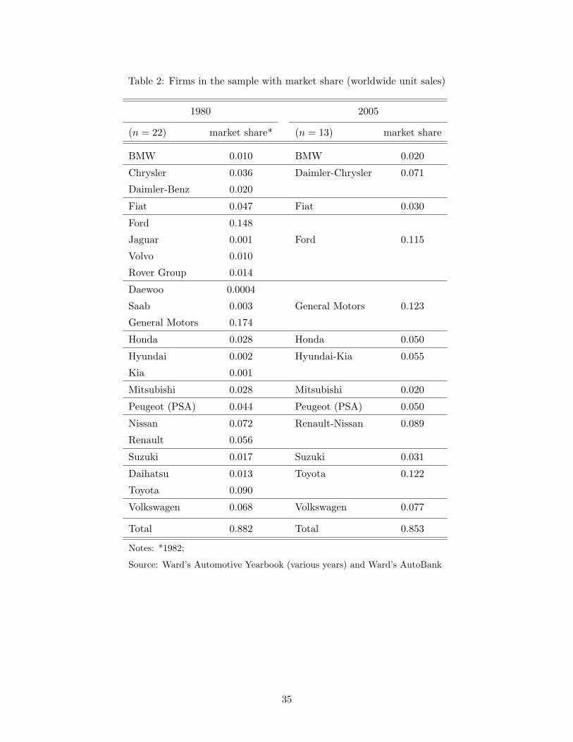
Table 2: Firms in the sample with market share (worldwide unit sales)

1980 2005

(n = 22) market share* (n = 13) market share

BMW 0.010 BMW 0.020

Chrysler 0.036 Daimler-Chrysler 0.071

Daimler-Benz 0.020

Fiat 0.047 Fiat 0.030

Ford 0.148

Jaguar 0.001 Ford 0.115

Volvo 0.010

Rover Group 0.014

Daewoo 0.0004

Saab 0.003 General Motors 0.123

General Motors 0.174

Honda 0.028 Honda 0.050

Hyundai 0.002 Hyundai-Kia 0.055

Kia 0.001

Mitsubishi 0.028 Mitsubishi 0.020

Peugeot (PSA) 0.044 Peugeot (PSA) 0.050

Nissan 0.072 Renault-Nissan 0.089

Renault 0.056

Suzuki 0.017 Suzuki 0.031

Daihatsu 0.013 Toyota 0.122

Toyota 0.090

Volkswagen 0.068 Volkswagen 0.077

Total 0.882 Total 0.853

Notes: *1982;

Source: Ward’s Automotive Yearbook (various years) and Ward’s AutoBank

35

Table 3: Demand Parameter Estimates

The dependent variable is log market share

OLS IV IV

Knowledge (ln(1 + ω)) 0.22∗∗∗ 0.20∗∗∗ 0.20∗∗∗

(0.03) (0.04) (0.04)

Price (ln p) −1.11∗∗∗ −1.82∗ −2.62∗∗

(0.19) (0.96) (1.32)

Time Fixed-Effects No No Yes

R2 0.38 0.32 -

No. of observations 155 155 155

Note: The only instrument in columns (2) and (3) is the

sum of all rivals’ knowledge. All variables are normalized by GM.

Significant at the ∗∗∗ 1%, ∗∗ 5%, and ∗ 10% level.

Table 4: Average ξ’s

Firm Name Average ξ Firm Name Average ξ Firm Name Average ξ

BMW -0.06 Honda -0.47 Renault na

Chrysler -0.50 Hyundai -1.11 Renault-Nissan na

Daewoo na Hyundai-Kia na Rover Group na

Daihatsu na Jaguar na Saab na

Daimler-Benz 0.34 Kia na Suzuki -0.68

Daimler-Chrysler 0.16 Mitsubishi -0.72 Toyota 0.43

Fiat 0.94 Nissan -0.15 Volkswagon 0.73

Ford 0.55 Peugeot-Citroen 1.03 Volvo na

Note: All unobserved qualities are normalized annually by GM quality.

36

Table 5: Parameter Estimates for the Marginal Cost Function

Dependent variable is marginal cost (relative to GM)

OLS OLS OLS

Constant term 0.83∗∗∗ 0.90∗∗∗ 1.01∗∗∗

(0.03) (0.03) (0.04)

Knowledge (ω) −7.36 × 10−5∗∗∗

(2.05 × 10−5)

Log knowledge (log(1 + ω)) −0.03∗∗∗

(0.01)

R2

No. of observations

Note: Significant at the ∗∗∗ 1%, ∗∗ 5%, and ∗ 10% level.

Table 6: Policy Function Estimates

Dependent variable is the number of new patents awarded

Independent Variable OLS OLS OLS

(without outliers) (without outliers)

Own Patent Stock 0.19∗∗∗ 0.28∗∗∗ 0.28∗∗∗

(0.02) (0.02) (0.01)

Own Patent Stock Squared −9.04 × 10−6 −5.55 × 10−5∗∗∗ −5.51 × 10−5∗∗∗

(7.38 × 10−6) (7.41 × 10−6) (6.21 × 10−6)

Sum of Rivals’ Patent Stocks −1.64 × 10−3∗ −2.48 × 10−3∗∗∗ −2.46 × 10−3∗∗∗

(9.39 × 10−4) (7.54 × 10−4) (7.33 × 10−4)

Own Rank −1.60∗ 0.07 −(0.97) (0.80)

R2 0.80 0.84 0.84

No. of observations 491 485 485

Note: Significant at the ∗∗∗ 1%, ∗∗ 5%, and ∗ 10% level.

37

Table 7: List of Abbreviations

Abrvn Firm Name Abrvn Firm Name Abrvn Firm Name

BMW BMW GMS General Motors PSA Peugeot-Citrion

CHR Chrysler HND Honda REN Renault

DBZ Daimler-Benz HYK Hyundai-Kia ROV Rover Group

DCH Daimler-Chrysler HYU Hyundai SAB Saab

DSU Daihatsu JAG Jaguar SZK Suzuki

DWO Daewoo KIA Kia TYO Toyota

FIA Fiat MTB Mitsubishi VOL Volvo

FRD Ford NSN Nissan VOW Volkswagon

Table 8: Merger Sequence 1

Period Merging Firms

2 CHR(139) NSN(674)

3 KIA(0) ROV(0)

4 DWO(0) FRD(443)

5 REN(12) DWO FRD

6 JAG(0) TYO(781)

7 VOL(3) KIA ROV

9 SAB(43) JAG TYO

11 SZK(6) VOL KIA ROV

13 FIA(0) SZK VOL KIA ROV

14 REN DWO FRD FIA SZK VOL KIA ROV

18 HYU(0) REN DWO FRD FIA SZK VOL KIA ROV

20 VOW(179) SAB JAG TYO

24 DSU(7) GMS(1189)

27 CHR NSN VOW SAB JAG TYO

50 PSA(0) MTB(199)

53 HYU REN DWO FRD FIA SZK VOL KIA ROV DSU GMS

56 BMW(28) HYU REN DWO FRD FIA SZK VOL KIA ROV DSU GMS

Notes: (1) Numbers in parenthesis are the first period (i.e. 1980) knowledge

stocks.

(2) Names in boxes are the firms that had merged before the current period .

(3) See Table 7 for the list of abbreviations.

38

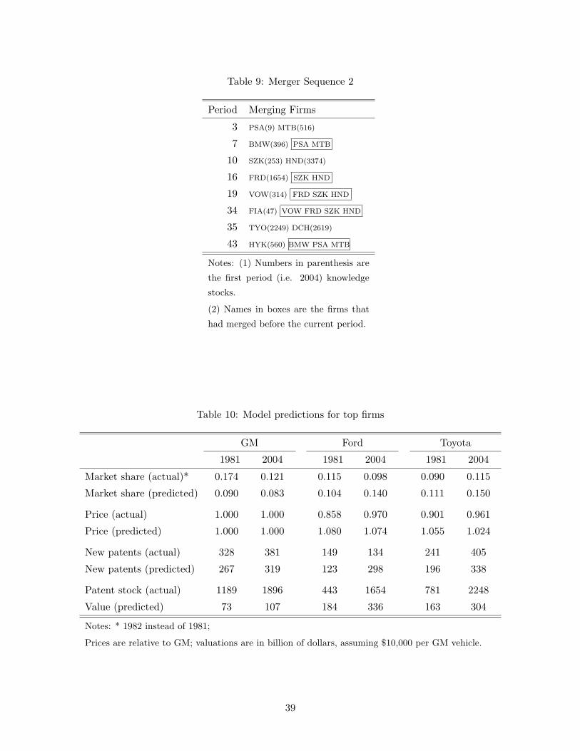
Table 9: Merger Sequence 2

Period Merging Firms

3 PSA(9) MTB(516)

7 BMW(396) PSA MTB

10 SZK(253) HND(3374)

16 FRD(1654) SZK HND

19 VOW(314) FRD SZK HND

34 FIA(47) VOW FRD SZK HND

35 TYO(2249) DCH(2619)

43 HYK(560) BMW PSA MTB

Notes: (1) Numbers in parenthesis are

the first period (i.e. 2004) knowledge

stocks.

(2) Names in boxes are the firms that

had merged before the current period.

Table 10: Model predictions for top firms

GM Ford Toyota

1981 2004 1981 2004 1981 2004

Market share (actual)* 0.174 0.121 0.115 0.098 0.090 0.115

Market share (predicted) 0.090 0.083 0.104 0.140 0.111 0.150

Price (actual) 1.000 1.000 0.858 0.970 0.901 0.961

Price (predicted) 1.000 1.000 1.080 1.074 1.055 1.024

New patents (actual) 328 381 149 134 241 405

New patents (predicted) 267 319 123 298 196 338

Patent stock (actual) 1189 1896 443 1654 781 2248

Value (predicted) 73 107 184 336 163 304

Notes: * 1982 instead of 1981;

Prices are relative to GM; valuations are in billion of dollars, assuming $10,000 per GM vehicle.

39

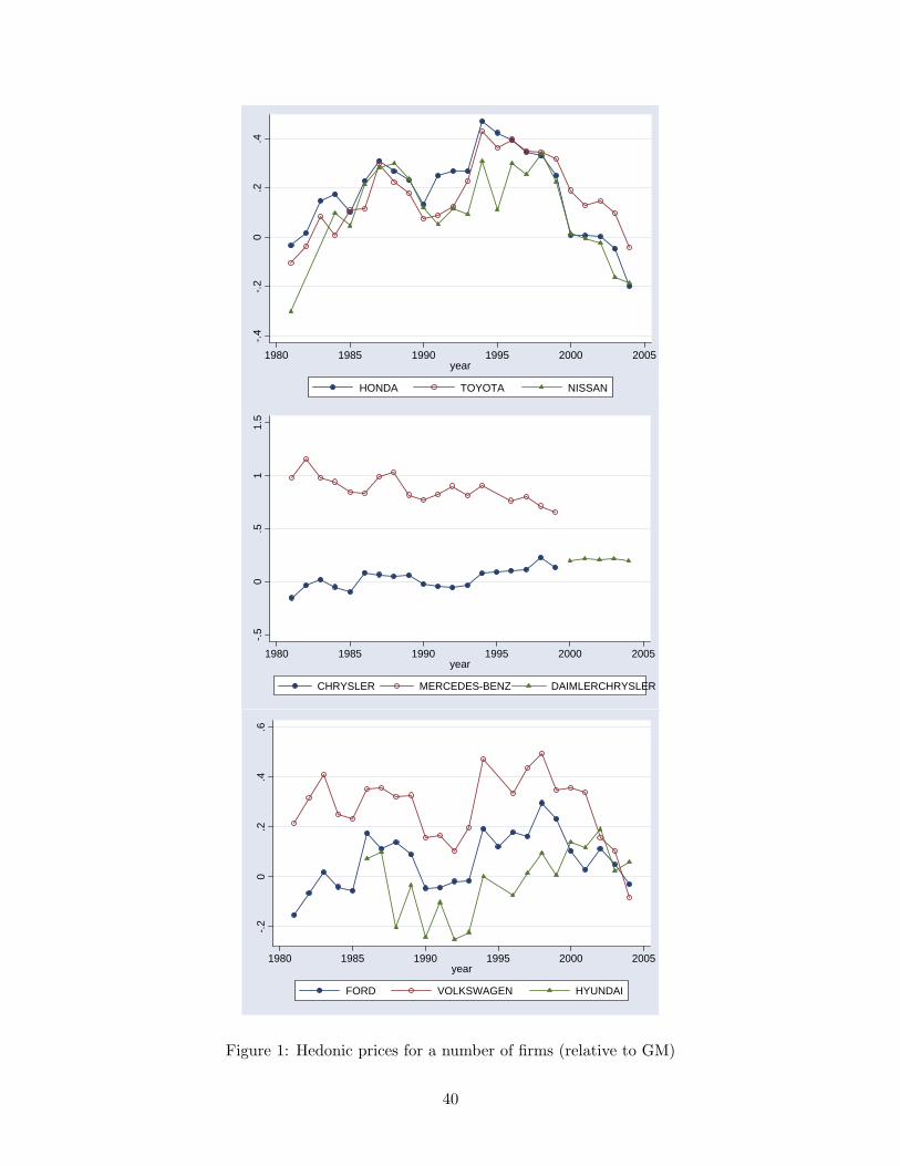
-.4-.2

0.2

.4

1980 1985 1990 1995 2000 2005year

HONDA TOYOTA NISSAN

-.50

.51

1.5

1980 1985 1990 1995 2000 2005year

CHRYSLER MERCEDES-BENZ DAIMLERCHRYSLER

-.20

.2.4

.6

1980 1985 1990 1995 2000 2005year

FORD VOLKSWAGEN HYUNDAI

Figure 1: Hedonic prices for a number of firms (relative to GM)

40

0 500 1000 1500 2000 2500 3000 35000

0.2

0.4

0.6

0.8

1

1.2

1.4

1.6

1.8

2

Patent Stock

Mar

gina

l Cos

t

Figure 2: Marginal Cost and Patent Stock

0 500 1000 1500 2000 2500 3000 35000

100

200

300

400

500

600

700

800

900

Patent Stock

Pate

nts

Issu

ed D

urin

g th

e Y

ear

Figure 3: Patents and Patent Stock

41

1980 1985 1990 1995 20000

200

400

600

800

1000

1200

data

model

Average of Firm ω (by Year)

Year

Ave

rge

ω

1980 1985 1990 1995 2000

400

600

800

1000

1200

data

model

Standard Deviation of Firm ω (by Year)

Year

Stan

dard

Dev

iatio

n ω

Figure 4: Evolution of ω’s: Model (average of 30 random sequences of mergers) and Data

42

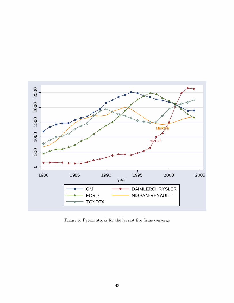
MERGE

MERGE

050

010

0015

0020

0025

00

1980 1985 1990 1995 2000 2005year

GM DAIMLERCHRYSLERFORD NISSAN-RENAULTTOYOTA

Figure 5: Patent stocks for the largest five firms converge

43

0.45

0.5

0.55

0.6

0.65

0

0.050.

1

0.150.

2(a

)

Firm

−le

vel C

ompe

titio

n (m

c/p)

Innovation Intensity

0.54

0.56

0.58

0.6

0.62

0.04

0.05

0.06

0.07

0.08

0.090.

1(b

)

Indu

stry

−le

vel C

ompe

titio

n (m

c/p)

Innovation Intensity

0.7

0.75

0.8

0.85

0.9

0.95

10

0.050.

1

0.150.

2(c

)

1−F

irm M

arke

t Sha

re

Innovation Intensity

0.8

0.85

0.9

0.95

10.

04

0.05

0.06

0.07

0.08

0.090.

1(d

)

1−H

erfin

dhal

Innovation Intensity

Fig

ure

6:C

ompe

titi

onan

dIn

nova

tion

atth

eFir

man

dIn

dust

ryLev

el

44

010

2030

4050

600.

54

0.56

0.580.

6

0.62

(a)

Tim

e P

erio

d

Industry−Level Competition (mc/p)

010

2030

4050

60468101214

x 10

11(b

)

Tim

e P

erio

d

Aggregate Industry Sales

010

2030

4050

6024681012

x 10

10(c

)

Tim

e P

erio

d

Aggregate Industry R&D

010

2030

4050

600.

04

0.05

0.06

0.07

0.08

0.090.

1(d

)

Tim

e P

erio

d

Innovation Intensity in the Industry

Fig

ure

7:C

ompe

titi

onan

dIn

nova

tion

over

Tim

e,W

ith

and

Wit

hout

Mer

gers

(Ind

ustr

yLev

el)

45

0.45

0.5

0.55

0.6

0.65

0

0.050.

1

0.150.

2(a

)

Firm

−le

vel C

ompe

titio

n (m

c/p)

Innovation Intensity

0.54

0.55

0.56

0.57

0.58

0.59

0.6

0.04

0.06

0.080.

1

0.12

0.14

(b)

Indu

stry

−le

vel C

ompe

titio

n (m

c/p)

Innovation Intensity

0.7

0.75

0.8

0.85

0.9

0.95

10

0.050.

1

0.150.

2(c

)

1−F

irm M

arke

t Sha

re

Innovation Intensity

0.82

0.84

0.86

0.88

0.9

0.92

0.04

0.06

0.080.

1

0.12

0.14

(d)

1−H

erfin

dhal

Innovation Intensity

Fig

ure

8:C

ompe

titi

onan

dIn

nova

tion

atth

eFir

man

dIn

dust

ryLev

elw

hen

the

Indu

stry

isC

once

ntra

ted

inth

eIn

itia

lSt

ate

46

010

2030

4050

0.54

0.55

0.56

0.57

0.58

0.590.

6(a

)

Tim

e P

erio

d

Industry−Level Competition (mc/p)

010

2030

4050

56789101112x

1011

(b)

Tim

e P

erio

d

Aggregate Industry Sales

010

2030

4050

5

5.56

6.57

7.58

8.5

x 10

10(c

)

Tim

e P

erio

d

Aggregate Industry R&D

010

2030

4050

0.04

0.06

0.080.

1

0.12

0.14

(d)

Tim

e P

erio

d

Innovation Intensity in the Industry

Fig

ure

9:C

ompe

titi

onan

dIn

nova

tion

over

Tim

e(I

ndus

try

Lev

el)

47

1998 2000 2002 2004 2006 2008 2010 2012 2014 2016

0.5

1

1.5

2

2.5

3

3.5

4x 10

11

sum of DBZ and CHR values w/o merger

DBZ value w/o merger

combined value after merger

CHR value w/o merger

(a) Daimler−Benz and Chrysler Values (w/ and w/o mergers)

Year

Val

ue

1998 2000 2002 2004 2006 2008 2010 2012 2014 20162

2.2

2.4

2.6

2.8

3x 10

12

with merger

without merger

(b) Industry Values (w/ and w/o mergers)

Year

Val

ue

Figure 10: The Effects Daimler-Benz and Chrysler Merger on Firm and Industry Values

48

2000 2005 2010 20150

2

4

6

8x 10

10

sum of HYU and KIA values w/o merger

KIA value w/o merger

combined value after merger

HYU value w/o merger

(a) Hyundai and Kia Values (w/ and w/o mergers)

Year

Val

ue

2000 2005 2010 20152.6

2.65

2.7

2.75

2.8

2.85

2.9x 10

12

without mergerwith merger

(b) Industry Values (w/ and w/o mergers)

Year

Val

ue

Figure 11: The Effects of Hyundai-Kia Merger on Firm and Industry Values

49

2005 2010 2015 20201

2

3

4

5

6

7x 10

11

sum of RNS and FRD values w/o merger

FRD value w/o merger

combined value after merger

RNS value w/o merger

(a) Renault−Nissan and Ford Values (w/ and w/o merger)

Year

Val

ue

2005 2010 2015 20202.45

2.5

2.55

2.6

2.65

2.7

2.75

2.8

2.85x 10

12

with merger

without merger

(b) Industry Values (w/ and w/o merger)

Year

Val

ue

Figure 12: The Effects of Renault-Nissan and Ford Merger on Firm and Industry Values

50

10 20 30 40 500.2

0.3

0.4

0.5w/o merger

w/ merger

(a) Daimler−Benz and Chrysler Merger and Utility

Period

Avg

Util

ity

10 20 30 40 500.3

0.4

0.5

0.6

0.7w/ merger

w/o merger

(b) Hyundai and Kia Merger and Utility

Period

Avg

Util

ity

10 20 30 40 500.45

0.5

0.55

0.6

0.65w/o merger

w/ merger

(c) Renault−Nissan and Ford Merger and Utility

Period

Avg

Util

ity

Figure 13: Mergers and Average Utility

51