Market quality in the time of algorithmictrading

Nidhi Aggarwal∗ Susan Thomas

December 19, 2013

Abstract

We contribute to the emerging literature on the impact of algo-rithmic trading with an analysis of India’s National Stock Exchange.This analysis has three strengths: A clean setting with one dominantexchange, a natural experiment where the introduction of co-locationwas followed by a sharp surge in algorithmic trading, and precise iden-tification of algorithmic orders and trades. The results largely suggestthat increased algorithmic intensity has given improvements of marketquality.

∗The authors are with the Finance Research Group, IGIDR. We are grateful to theNational Stock Exchange of India, Ltd. for both research support. We thank Ajay Shahfor inputs into the research design and Chirag Anand for technological inputs.

1

Contents

1 Introduction 3

2 The impact of algorithmic trading (AT) on markets 4

3 Research setting 63.1 A clean microstructure . . . . . . . . . . . . . . . . . . . . . . 63.2 The introduction of the co-location facility (co-lo) . . . . . . . 73.3 A unique dataset . . . . . . . . . . . . . . . . . . . . . . . . . 8

4 Measurement 84.1 Measuring AT intensity . . . . . . . . . . . . . . . . . . . . . . 84.2 Measuring market quality . . . . . . . . . . . . . . . . . . . . 9

4.2.1 Liquidity . . . . . . . . . . . . . . . . . . . . . . . . . . 94.2.2 Volatility . . . . . . . . . . . . . . . . . . . . . . . . . 114.2.3 Market efficiency . . . . . . . . . . . . . . . . . . . . . 11

5 Methodology 125.1 Co-location and AT intensity . . . . . . . . . . . . . . . . . . 125.2 Choice of samples . . . . . . . . . . . . . . . . . . . . . . . . . 125.3 Threats to validity: did other factors cause changes in market

quality? . . . . . . . . . . . . . . . . . . . . . . . . . . . . . . 15

6 Data 19

7 Results 217.1 How did AT impact market quality? . . . . . . . . . . . . . . 217.2 Threats to validity: Did other factors cause the change in

market quality? . . . . . . . . . . . . . . . . . . . . . . . . . . 25

8 Conclusion 29

A Estimations addressing threats to validity 32

2

1 Introduction

In recent years, there has been a surge of interest in the impact of algorithmictrading (AT) upon market quality. In this paper, we examine the impact ofAT upon market quality at the National Stock Exchange of India (NSE),which is one of the biggest exchanges of the world, with India as a largeemerging market. In addition, this paper improves upon existing measure-ment of the role of AT through clean identification of the impact of AT uponmarket quality, owing to a research design with three unique features.

The first concerns fragmentation of the order flow. In countries such as theUS, trading takes place at numerous venues, each of which has a differentmarket design. This makes it hard to understand the causal impact of onedesign feature such as algorithmic trading at any one trading venue. Incontrast, in our study of NSE, we have a simple setting where NSE accountsfor 80% of equity spot trading and 100% of equity derivatives trading.

The second issue is about disentangling cause and effect where traders volun-tarily shift to algorithmic trading. At NSE, there was a sharp date in January2010 on which the co-location facility was commissioned, after which therewas an S-curve adoption of AT. This gives us a dataset with one group ofdays (prior to the co-location facility) with AT intensity of 15%, and anothergroup of days (after the co-location facility) with AT intensity of 55%.

The third issue is about measurement. Many researchers have been forced towork with crude proxies of algorithmic trading. The data at NSE preciselyflags every order, and counterparties on every trade, as being AT or not.

The analysis shows that, on average, market quality has improved in thefollowing ways: lower transactions costs, larger number of shares availablefor trade, and a reduced imbalance between the number of shares availableto buy and sell. It also shows a sharp drop in the volatility of prices andthe volatility of transactions costs after the increase in algorithmic trading.However, the depth as measured by the monetary value available to tradeworsens with higher algorithmic trading, both at the touch (best bid andoffer) as well as the value available for trading upto the best 5 prices decreases.These results are similar to the findings of Hendershott et al. (2011), whofind that increased algorithmic trading activity in the US caused a drop inquoted as well as effective spreads, but also lowered the quoted depth. Otherthan the depth measures, these results do suggest that, on average, marketquality improved with algorithmic trading.

A key threat to validity of the analysis lies in changing macro-economic

3

conditions. The pre-co-location period happens to lie in 2009, which wasa time of enhanced macroeconomic uncertainty. This raises the possibilitythat some or all of the apparent improvements in market quality were merelydriven by restoration of normalcy in finance and macroeconomics.

We address these concerns through two strategies. First, financial and macroe-conomic uncertainty is controlled for in linear regressions. Second, a matcheddataset is constructed containing days which have similar aggregate volatil-ity. This is equivalent to controlling for aggregate volatility, without assum-ing linearity of the relationship between volatility and market quality. Thisanalysis shows that results that are consistent with the earlier analysis inall but the order imbalance which is the difference in the number of sharesavailable to buy and sell. Here, the estimations (after adjusting for macroe-conomic volatility) show that there was no significant impact of algorithmictrading on the order imbalance. Thus, we conclude that algorithmic tradingimproves market quality, other than the depth measures.

The remainder of the paper is organised as follows: Section 3 provides a briefdetail on the institutional framework. Section 5 discusses the identificationof algorithmic trading activity, measurement of market quality measures andthe approach used for analysis in detail. Section 6 describes the data andgives some summary statistics. Section 7 presents the estimation results.Section 8 concludes.

2 The impact of algorithmic trading (AT) on

markets

Algorithmic Trading (AT) has been defined as the use of computer algorithmsto automatically make trading decisions, submit orders and manage thoseorders after submission (Hendershott et al., 2011). Many researchers havetried to understand how this shift in the use of technology has changed marketquality in terms of liquidity, price efficiency and volatility.

Theoretical models focus on a subset of AT called high frequency trading(HFT), which has a greater focus on low latency of order placement. Thesemodels analyse how a rapidly changing trading environment affects liquiditycosts and investor welfare. Jovanovic and Menkveld (2010) suggest that tothe extent that information is known only to the HFTs, they can reduce wel-fare. However, in markets where information is continually updated, HFTcan improve welfare by posting competitive quotes and reducing informa-

4

tional friction. Biais et al. (2013) show that the rapidity of order placementcan have a positive impact by providing mutual gains from trade, but alsocause negative externalities by increasing adverse selection cost. Cartea andPenalva (2012) build on Grossman and Miller (1988) and show that presenceof HFT makes liquidity traders worse off by increasing the price impact oftheir trade as well as the volatility of the prices. On the other hand, Hoff-mann (2012) modifies Foucault (1999) to show how HFT can have a positiveimpact on market liquidity, conditional on the initial level of market effi-ciency. Martinez and Rosu (2013) show that HFT does not destabilise themarkets, but improves market efficiency by incorporating information intoprices quickly.

The dominant strand in the AT literature is empirical measurement of theimpact of AT. A major drawback in this literature is poor measurement.Most existing datasets do not have precise flagging of orders or trades thatuse AT. Zhang (2010) uses a proxy to observe HFT and finds that highfrequency trading is negatively related to price formation and also increasevolatility. Hasbrouck and Saar (2013) develop a new proxy based on strate-gic runs in the market, and finds that with increased high frequency trad-ing comes narrower spreads, higher displayed depth and lowered short termvolatility. Hendershott et al. (2011) treats electronic messages as a proxy forAT, and uses the onset of automated quote dissemination on the New YorkStock Exchange as an exogenous event. They find that AT lowers liquid-ity costs, and improves quote informativeness, particularly for large marketcapitalization securities.

Another approach to identification is to locate market wide events that areexpected to change the level of AT intensity, or exogenous factors indicatingthe degree of AT in the market. For example, Riordan and Storkenmaier(2012) use the drop in latency at the Deutsche Bourse and find that it iscorrelated with improved market quality measured by decreased spreads andhigher price efficiency.1 Bohemer et al. (2012) use the introduction of co-location facilities at 39 exchanges to locate increases in the level of AT inmarkets and find that higher AT is correlated with better market liquidity,efficiency, but also higher market volatility. In contrast, Chaboud et al.(2009) find no similar relationship between AT and higher volatility on foreignexchange markets.2

1A few studies such as Viljoen et al. (2011), Frino et al. (2013) also examine theimpact of algorithmic trading on the futures market. They find a similar positive impactof algorithmic trading on liquidity and price efficiency.

2Other studies also look at the liquidity provisioning function of algorithmic traders.Hendershott and Riordan (2013) find that algorithmic traders demand liquidity when it is

5

In the best scenario, researchers access proprietary datasets to examine therole of high frequency traders (HFTs, which is a subset of AT) on pricediscovery and efficiency. For example, Menkveld (2013), Carrion (2013),Brogaard (2010), Brogaard et al. (2012), find that HFTs play a beneficialrole in enabling price efficiency and provide liquidity, particularly aroundtimes of market stress.

There is a certain contrast between the broadly benign messages of the re-search literature, and the mistrust that many policy makers and practitionersexpress about the role of AT. The limitations of the datasets used in the exist-ing literature have generated skepticism about the existing literature. In thispaper, we analyse a large exchange with perfect identification of algorithmicorders and trades.

3 Research setting

The research setting in this paper has three strengths compared with the restof the literature. There is a clean market microstructure setting where mostspot trading and all derivatives trading takes place at only one exchange;there is a natural experiment where AT surged after co-location facilities wereintroduced on this exchange; the underlying data infrastructure preciselyflags every order and the counterparties of every trade with a dummy variablesignifying AT.

3.1 A clean microstructure

We analyse the impact of AT on market quality of one of three exchangestrading equity in India,3 the National Stock Exchange (NSE). NSE has thelargest share of the domestic market activity, with 80% of the traded vol-umes on the equity spot market and 100% of the traded volume on equityderivatives (SEBI, 2013). It is also one of the highest ranked equity marketsin the world by transaction intensity.4

cheap and supply liquidity when it is expensive. Carrion (2013) study the high frequencytrading strategies and find that HFTs provide liquidity when it is scarce and consumewhen it is plentiful.

3The other two are the Bombay Stock Exchange and Multi-commodity Stock Exchange.4Source:http://www.world-exchanges.org/files/statistics/2012%20WFE%

20Market%20Highlights.pdf

6

The NSE is an electronic limit order book market, where orders are executedon a price-time priority basis. Information about trades, quotes, and quanti-ties are disseminated by the exchange on a real time basis, with traders beingable to view the best five bid-ask prices at every given point in time. Thereare around 1500 securities that trade on the NSE. Current trading hours arefrom 9:00 am to 3:30 pm (IST), but were from 9:55 am to 3:30 pm before Jan1, 2010. The market opens with a call auction which runs for 15 minutes,after which trading is done using a continuous order matching system.

All spot trades are cleared with netting by novation at a clearing corporationand settled on a T + 2 basis. Netting within the day accounts for roughly70% of the turnover. Of the trades that are settled, typically around 10-15%have a domestic and foreign institutional investor. Most of the trading canbe attributed to retail investors or proprietary trading by securities firms.

3.2 The introduction of the co-location facility (co-lo)

In the international experience, computer technology came into order place-ment owing to the desire to achieve best execution for customers.5 This wasnot a consideration in India, where NSE was and has been the dominantexchange, and there have been no regulations about best execution.

Automated order placement began with a few securities firms establishingtechnology for equity spot arbitrage between NSE and BSE. The securitiesregulator issued regulations governing algorithmic trading in April 20086 buteven after this, the level of AT remained low.7

The decisive event was co-location at NSE,w hich began in January 2010.8

Latency dropped from 10–30 ms to 2–6 ms, and traders who establishedautomated systems in the co-location facility had a significant edge. Thisgave a surge in AT, as is documented later in this paper.

5Some examples of this include Marketplace rules, 2001 by the Canadian SecuritiesAdministration, Regulation National Market Services or Regulation NMS, 2005 by theU.S. SEC and Markets in Financial Instruments Directive or MiFID, 2007 in Europe.

6http://www.sebi.gov.in/circulars/2008/cir072008.pdf7http://www.livemint.com/Opinion/QpU7GHjhTLwClANyUX5T5N/

Indian-markets-slowly-warming-up-to-algorithmic-trading.html8http://www.nseindia.com/technology/content/tech_intro.htm

7

3.3 A unique dataset

The previous literature examining the impact of AT or HFT has generallybeen limited to observing proxies for AT. For example, Hendershott et al.(2011) and Bohemer et al. (2012) use electronic message traffic to capturethe level of algorithmic trading activity in the market, Hasbrouck and Saar(2013) propose a measure called RunsInProcess to identify HFT activity.

The closest that the literature has to a direct measure is where the exchangeidentifies trading firms as ‘engaging primarily in high frequency trading’.Therefore, Brogaard (2010), Brogaard et al. (2012) and Carrion (2013) usedata from NASDAQ that identifies a subset of HFT on a randomly selected120 US securities based on the activity of 26 trading firms tagged by NAS-DAQ as being engaged in HFT. Despite being a very informative dataset,there are concerns about the coverage of the HFT firms in the sample (Bro-gaard et al., 2012; Bohemer et al., 2012). Another study by Hendershottand Riordan (2013) uses DAX dataset on AT orders for 30 securities on 13trading days. While this does not suffer from the problem of coverage of ATfirms, it suffers from the issue of very small sample that covers only a fewsecurities.

Our analysis uses a dataset of all orders and all trades, timestamped to themillisecond, with an AT flag for every order and for every counterparty ofevery trade. This data is available from 2009 onwards, which covers theperiod before the co-location facility also. This is thus a unique datasetwithin the AT literature.

4 Measurement

As with the rest of the literature, there are two main issues that shape theresearch design. The first group of questions is about measuring AT intensityand market quality. The second group of questions is about establishing acausal impact of AT intensity upon market quality.

4.1 Measuring AT intensity

We classify a trade as an AT trade if either buyer or seller was AT. High-frequency data is used to construct a discrete measure, with a resolution offive minutes, of AT intensity. The AT intensity, at-intensityi,t, for any

8

security ‘i’ in any given time interval ‘t’, is the share of AT trades withintotal traded value within the five-minute interval:

at-intensityi,t =ttvATtrade,i,t × 100

ttvi,t

where ttvATtrade,i,t refers to the total traded value of AT trades in timeperiod ‘t’. TTVi,t refers to total traded value of all trades in time period ‘t’.

4.2 Measuring market quality

Liquidity, volatility and market efficiency are measures of market quality,with precise definitions as follows.

4.2.1 Liquidity

Liquiditiy is multi-dimensional in nature, and so we break up measurementinto two parts: transactions costs and depth. Transactions costs are higherfor markets that are less liquid. Depth is lower for markets that are lessliquid. We use the following measures to capture market liquidity:

1. Transactions costs measures:

a) Quoted Spread (qspread): It is measured as the difference betweenthe best ask and the best bid price at any given point of time. In orderto make it comparable across securities, we express it as a percentageof the mid-quote price, which is the average of the best bid and theask prices. Thus, for a security ‘i’ at time ‘t’, qspreadi,t is defined as

qspreadi,t =(PBestAski,t − PBestBidi,t)× 100

PMQi,t

where PBestAski,t and PBestBidi,t are the best ask and bid prices respec-tively. PMQi,t indicates the mid-quote prices.

b) Impact Cost (ic): The qspread only captures the liquidity availableat the best prices. However, the transaction size supported at the bestprice may not be the typical size at which traders typically executetheir trades. Instead, we use the Impact Cost, which measures liquidity

9

for a fixed transaction size Q. For a security ‘i’, at time ‘t’, ICQ,i,t iscalculated as:

icQi,t = 100×PQi,t − PMQi,t

PMQi,t

where PQi,tis the execution price calculated for a market order of Q

and PMQi,tis the mid-quote price. Q is held fixed at a transaction size

of USD 500 (Rs 25,000).9

Lower values of qspread and ic indicate higher liquidity.

2. Depth (depth) measures:

a) top1depth captures the rupee depth at the best bid and ask pricesas:

top1depthi,t = PBestBid,i,t ×QBestBid,i,t + PBestAsk,i,t ×QBestAsk,i,t

where PBestAski,t and PBestBidi,t are the best ask and bid prices respec-tively of security ‘i’ at time ‘t’.

b) top5depth captures the cumulated rupee depth across the best fivebid and ask prices as:

top5depthi,t = Σ5k=1PBestBid,k,i,t×QBestBid,k,i,t+Σ5

k=1PBestAsk,k,i,t×QBestAsk,k,i,t

where PBestAski,t and PBestBidi,t are the best ask and bid prices of se-curity ‘i’ at time ‘t’.

c) Depth measure the total number of shares outstanding at either sideof the book available for execution at any point of time. It is expressedas an average, with units of number of shares, and is computed as:

depthi,t =TSQi,t + TBQi,t

2

where TSQi,t denotes the total sell quantity and TBQi,t denotes thetotal buy quantity of security ‘i’ at time ‘t’.

d) Order Imbalance (oib) is measured as the difference between the buyand sell side depth, and expressed as a percentage of the total depthon average as:

OIBi,t =(TSQi,t − TBQi,t)× 200

TBQi,t + TSQi,t

A market with lower absolute value of order imbalance is viewed as ahigh quality market.

9This is the average transaction size on the spot market at NSE.

10

4.2.2 Volatility

There are two elements of volatility observed from market prices: price andliquidity risk.

1. Price risk (rvol): This is the variance of intra-day returns, where returnsare calculated using traded prices at one second frequency as:

rvoli,t =

√Σ300T=1(ri,T − ri,t)2

n− 1

where ‘t’ indexes the five minutes time interval, while ‘T ’ indexes the onesecond time points. ri,T indicates the mean returns within the five minuteinterval.

2. Liquidity risk (lrisk): We measure liquidity risk as the variance of impactcost over a given time interval. It captures the variation in the transactionscosts faced when executing a market order of size Q at different times in thetrading day.

lrisk is computed as the standard deviation of IC (computed at one-secondfrequency) in a five minute interval:

lriski,t =

√Σ300T=1(ici,T − ici,t)2

n− 1

where ‘t’ indexes the five minutes time interval, while ‘T ’ indexes the onesecond time points. ici,t indicates the mean of IC within the five minuteinterval.

4.2.3 Market efficiency

While there are several measures to calculate the efficiency of market prices,we use the Variance Ratio (vr) of returns. The variance ratio (Lo andMacKinlay, 1988) is defined as the ratio of 1/k times the variance of k-periodreturn to that of one period return, and is calculated as:

vr(k) =V ar[rt(k)]

k · V ar[rt]

where rt is the one period continuously compounded return, rt(k) = rt +rt−1 . . . + rt−k. k indicates the lag at which the variance ratio (vr)is to becomputed.

11

We compute the VR as the ratio of the variance of returns calculated overten minutes to the variance of five minute returns. In an efficient market,where prices are expected to approximate a random walk, these values of vrshould be not be significantly different from 1.

5 Methodology

We use two approaches to establish a causal relationship between the ATintensity and market quality: (a) An comparative analysis of the averagelevels of market quality between a period when AT was low to when AT washigh. (b) A cross-sectional analysis of the effect of AT on market quality atthe level of specific securities between the period of low and high AT.

5.1 Co-location and AT intensity

The introduction of co-location services at the NSE as described in Section3.2 can be a useful exogenous event which gives us an opportunity to measurethe impact of AT intensity upon market quality. Prior to the introductionat co-location services, the level of AT in the market was low.

While we expect a significant increase in the presence of AT trades andorders in the market, we expect that the change would come about throughthe typical S-curve of adoption of innovations.

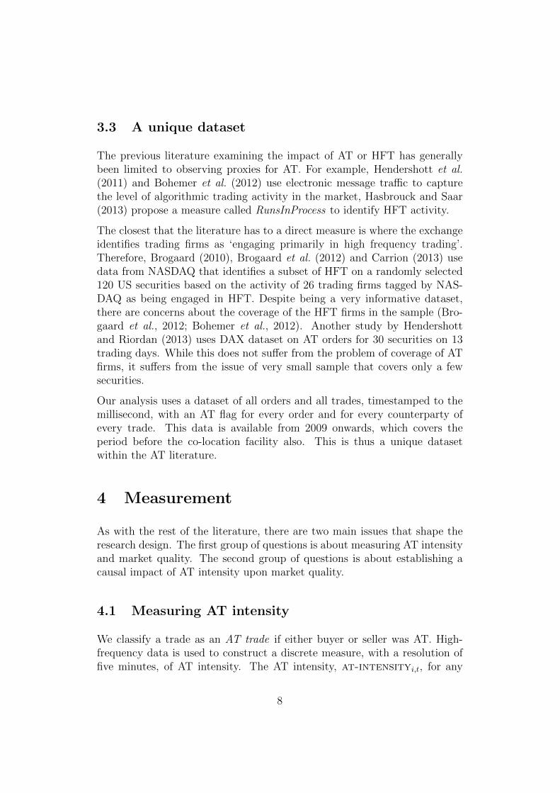
Figure 1 shows that before the introduction of the co-lo in January 2010, theAT intensity on the NSE was low. After the introduction of the co-lo (markedby the dashed vertical line in the graph), AT intensity picked up gradually.The period between January 2010 and July 2011 was an adjustment periodwhere participants were adopting the new technology.

This S-curve of adoption implies that it is not useful to do a sharp study ofa few days before and after the introduction of the co-location facility.

5.2 Choice of samples

We use Figure 1 to select two groups of days, one where the data shows alow level of at-intensity and another where at-intensity is significantlyhigher. Before January 2010, the average AT intensity was at around 20%.After January 2010, at-intensity steadily increased through but stabilized

12

Figure 1 AT intensity between 2009 and 2013

The graph shows AT intensity for the overall equity spot market at NSE between 2009and 2013. AT intensity is measured as a fraction of total traded value of AT trades in aday vis-a-vis the total traded value on that day. The dotted line shows the date on whichco-lo was introduced by NSE. The shaded region indicates the two periods of study.

2009 2010 2011 2012 2013

1020

3040

5060

70

AT In

tens

ity (

%)

Start ofco−loPre co−lo Post co−lo

2009 2010 2011 2012 2013

1020

3040

5060

70

AT In

tens

ity (

%)

at 50% after July 2011. Hence, we choose the following groups of days foranalysis:

• The low-AT sample: 9 July to 7 August 2009

• The high-AT sample: 9 July to 8 August 2012

We examine the average at-intensity of the overall market10 in each ofthe the selected samples in greater detail in Table 1. We also examine theat-intensity of the top 100 securities by market capitalisation.

We see that the average at-intensity for the overall market was about4.33% in the low-at sample. This is significantly higher in the high-atsample at 16.39%. In the universe of 100 large sized securities, we see thatthe average AT intensity in the low-at sample was significantly higher at14.28%, higher by nearly 4× of the overall market. This further rose to53.97% in the high-at sample, an increase of 3×.

10The ‘overall market’ consists all the securities traded on the NSE equity spot marketsduring this period. On average, NSE trades around 1500 securities daily.

13

Table 1 Summary statistics of AT intensity in the low-at and high-atperiods

The table presents summary statistics of at-intensity for the overall market and the top100 securities by market capitalization and liquidity.at-intensity is calculated as the percentage of the total traded value of AT trades vis-a-vis the total traded value for a security within a day. It is calculated for each security inthe low-at (July 6 to August 8, 2009) and high-at (July 6 to August 9, 2012) samplesseparately, and then averaged across all days.

All values in %Overall Market Top100low-at high-at low-at high-at

Min 0.00 0.00 2.36 22.91Q1 1.34 5.44 10.15 46.37Mean 4.10 16.39 14.28 53.97Median 2.33 12.07 14.34 55.14Q3 4.00 21.66 19.16 61.83Max 27.13 77.28 27.13 77.28SD 4.81 15.18 5.98 11.60

In addition to the comparative analysis of the average market quality, we usea fixed effects regression to adjust for the cross-sectional variation in marketquality in relation to the cross-sectional variation in AT intensity. This helpsto reduce the endogeneity bias induced as a result of omitted variables. Themodel used is as follows:

M1 : mkt-qualityi,t = αi + β1at-intensityi,t−1 + β2co-lo-dummyt + εi,t

where i = 1,. . . ,N indexes firms, t = 1,. . . ,T, indexes 5-minute time in-tervals. αi captures the firm specific unobserved factors, mkt-qualityi,t

represents one of the market quality measures (qspread, ic, top1depth,top5depth, oib, depth, lrisk, rvol) for security ‘i’ at time ‘t’. co-lo-dummyi,t is a dummy used to capture the differences due to differences inthe low-at and high-at samples. It takes value ‘1’ for the high-at sampleand zero otherwise. That is,

co-lo-dummyt =

{1 if ‘t’ ∈ Post 2010 period

0 otherwise

at-intensityi,t−1 represents the AT intensity in security ‘i’ in the previousfive minutes. We use the previous five minutes of at-intensity to address

14

the endogeneity issues that can arise because of the feedback relation betweenthe market quality variables and at-intensity. The coefficient of interestis β2 which captures the effect of AT on each market quality variable.

If higher at-intensity results in better market quality, we expect β2 tobe negative for the market quality variables qspread, ic, lrisk, |oib|,rvol and positive for depth, top1depth, top5depth. Thus, we test thehypothesis (H1

0):

H10 : β2 = 0

H1A : β2 < 0

where mkt-quality ∈ (qspread, ic, lrisk, |oib|, rvol).

We expect that better market quality is associated with higher depth, andset the alternative hypothesis to be:

H1A : β2 > 0

where mkt-quality ∈ depth, top1depth, top5depth.

Since the dataset is a panel with of large number of time-dimensional ob-servations, we report the Driscoll-Kraay standard errors which are robust toheteroskedasticity, autocorrelation and cross-sectional dependence (Driscolland Kraay, 1998; Hasbrouck and Saar, 2013).

5.3 Threats to validity: did other factors cause changesin market quality?

In Section 5.2, we selected samples before and after the introduction of co-losuch that AT intensity was significantly higher level in the high-at sample.However, as the two periods are three years apart, there is the possibility ofmany other things having changed. If market volatility is significantly differ-ent between the two samples, then the significant changes in market qualitymight be a consequence of market volatility rather than the change in AT.For example, the low-at sample is observed from the period immediatelyafter the 2008 global financial crisis where market volatility would tend tobe systematically higher compared to that in the high-at period, which iswell after the crisis.

A similar argument holds for liquidity measures. The literature on com-monality of liquidity across securities shows a significant influence of market

15

Figure 2 Market volatility and liquidity between 2009 and 2013

The first graph below shows the daily time series of the implied volatility index, IndiaVIX between 2009 and 2013, while the second graph shows the monthly time series of theimpact cost of buying and selling Rs.5 million (under USD 80,000) worth of the NSE-50index.The dashed line indicates the date on which NSE started co-lo services. The shaded regionsindicates the periods of the low-at and the high-at samples selected for the analysis.

2009 2010 2011 2012 2013

2030

4050

Indi

a V

IX (

%)

Start ofco−lo

2009 2010 2011 2012 2013

2030

4050

Indi

a V

IX (

%)

Pre co−lo Post co−lo

0.06

0.08

0.10

0.12

0.14

Nift

y IC

(%

)

2009 2010 2011 2012 2013

Start ofco−lo

0.06

0.08

0.10

0.12

0.14

Nift

y IC

(%

)

Pre co−lo Post co−lo

16

liquidity on the liquidity of all securities (Chordia et al., 2000), and in turn,market liquidity is strongly related to market volatility (Hameed et al., 2010).

We examine the time series of the volatility and liquidity of the market indexbetween January 2009 to August 2013. Market volatility is measured by thedaily time series of the Indian implied volatility index, India VIX,11 while themarket liquidity is measured by the monthly time series of the Nifty ImpactCost12 in the same period. The graphs shows that both market volatility wasmuch higher in 2009 compared to the 2013. The market impact cost was alsomuch higher showing that market liquidity was significantly lower during theselected low-at sample than the high-at sample.

We address this problem through two strategies.

1. Including conditioning variables in the models of cross-sectionalvariation: We add a control variable that captures market volatility inthe specification given by M1. The market volatility is measured using therealised volatilty of the Nifty index.13 This is used to modify M1 to give M2as follows:

mkt-qualityi,t = αi + β1co-lo-dummyt + β2at-intensityi,t−1

+β3nifty-volt + εi,t

where nifty-voli,t is the variance of five-minute returns on the marketindex.

In the aftermath of the global crisis, there were particularly sharp peaksof volatility within the day. In order to control for these, we introduce anintra-day dummy into M3:

mkt-qualityi,t = αi + β1co-lo-dummyt + β2at-intensityi,t−1

+β3nifty-volt + β4intraday-dummyt + εi,t

where the intraday-dummy takes value 1 if ‘t ’ is the first or the last halfhour of the trade, and zero otherwise. The selection of the first half an hour

11India VIX is a volatility index based on the Nifty Index Option prices. Nifty is NSE’smarket index based on 50 securities which constitute about 70% of the free float marketcaptialization of the securities listed on NSE. India VIX uses the Chicago Board OptionsExchange (CBOE) computation methodology, with few amendments to suit the Indianmarkets. See: http://www.nseindia.com/content/indices/white_paper_IndiaVIX.

pdf12Nifty Impact Cost represents the cost incurred on buying or selling a portfolio of

Nifty stocks for a transaction size of Rs. 50 lacs (around USD 83,333). The numbers aredisseminated by the NSE on a monthly basis.

13Nifty is the market index comprising of the 50 largest firms (that are traded on NSE)in terms of market capitalization and transactions costs that are traded on NSE.

17

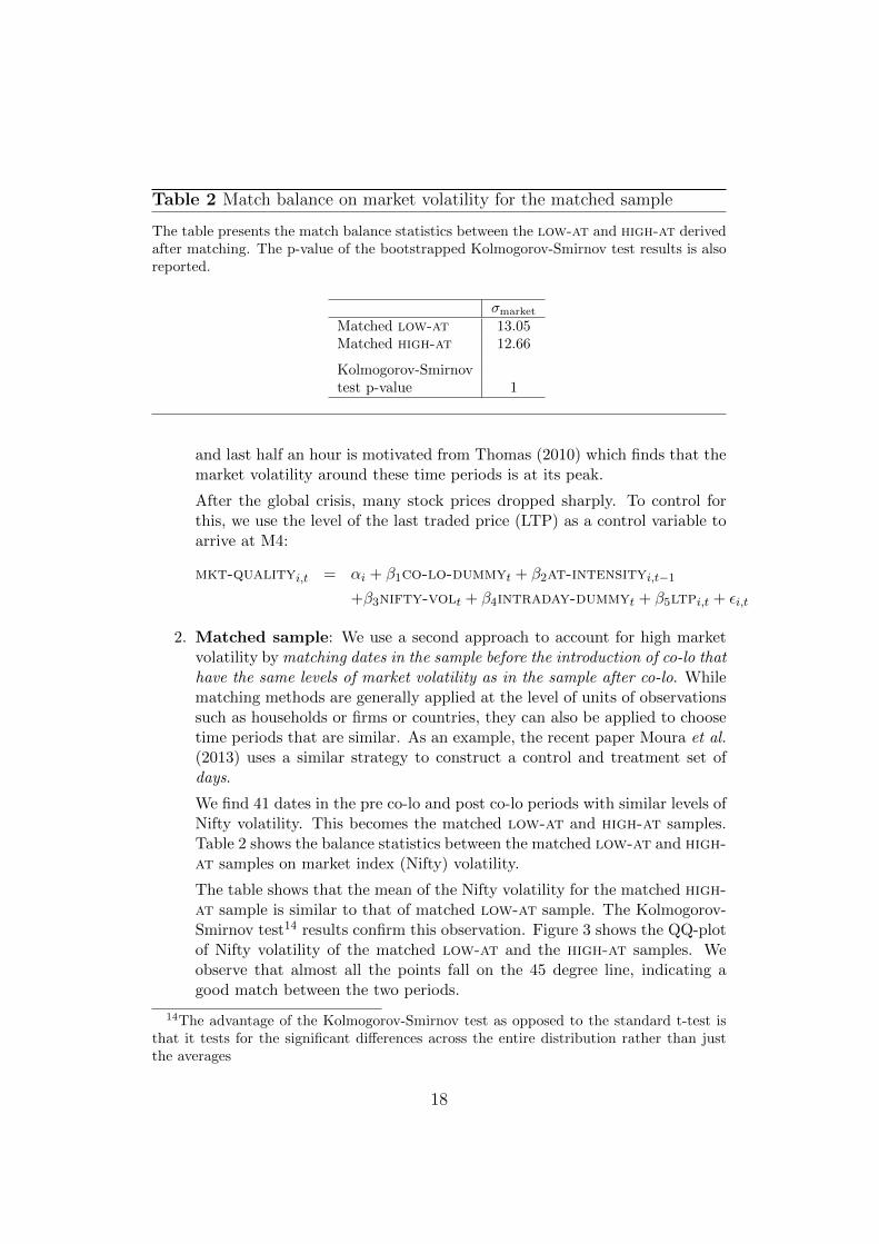
Table 2 Match balance on market volatility for the matched sample

The table presents the match balance statistics between the low-at and high-at derivedafter matching. The p-value of the bootstrapped Kolmogorov-Smirnov test results is alsoreported.

σmarket

Matched low-at 13.05Matched high-at 12.66

Kolmogorov-Smirnovtest p-value 1

and last half an hour is motivated from Thomas (2010) which finds that themarket volatility around these time periods is at its peak.

After the global crisis, many stock prices dropped sharply. To control forthis, we use the level of the last traded price (LTP) as a control variable toarrive at M4:

mkt-qualityi,t = αi + β1co-lo-dummyt + β2at-intensityi,t−1

+β3nifty-volt + β4intraday-dummyt + β5ltpi,t + εi,t

2. Matched sample: We use a second approach to account for high marketvolatility by matching dates in the sample before the introduction of co-lo thathave the same levels of market volatility as in the sample after co-lo. Whilematching methods are generally applied at the level of units of observationssuch as households or firms or countries, they can also be applied to choosetime periods that are similar. As an example, the recent paper Moura et al.(2013) uses a similar strategy to construct a control and treatment set ofdays.

We find 41 dates in the pre co-lo and post co-lo periods with similar levels ofNifty volatility. This becomes the matched low-at and high-at samples.Table 2 shows the balance statistics between the matched low-at and high-at samples on market index (Nifty) volatility.

The table shows that the mean of the Nifty volatility for the matched high-at sample is similar to that of matched low-at sample. The Kolmogorov-Smirnov test14 results confirm this observation. Figure 3 shows the QQ-plotof Nifty volatility of the matched low-at and the high-at samples. Weobserve that almost all the points fall on the 45 degree line, indicating agood match between the two periods.

14The advantage of the Kolmogorov-Smirnov test as opposed to the standard t-test isthat it tests for the significant differences across the entire distribution rather than justthe averages

18

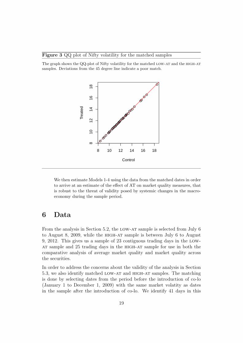
Figure 3 QQ plot of Nifty volatility for the matched samples

The graph shows the QQ-plot of Nifty volatility for the matched low-at and the high-atsamples. Deviations from the 45 degree line indicate a poor match.

●●●

●●●●●

●●●●

●●●●●●●●●●

●●●●●

●●●●●

●●●●

●●

●●

●

8 10 12 14 16 18

810

1214

1618

Control

Trea

ted

We then estimate Models 1-4 using the data from the matched dates in orderto arrive at an estimate of the effect of AT on market quality measures, thatis robust to the threat of validity posed by systemic changes in the macro-economy during the sample period.

6 Data

From the analysis in Section 5.2, the low-at sample is selected from July 6to August 8, 2009, while the high-at sample is between July 6 to August9, 2012. This gives us a sample of 23 contiguous trading days in the low-at sample and 25 trading days in the high-at sample for use in both thecomparative analysis of average market quality and market quality acrossthe securities.

In order to address the concerns about the validity of the analysis in Section5.3, we also identify matched low-at and high-at samples. The matchingis done by selecting dates from the period before the introduction of co-lo(January 1 to December 1, 2009) with the same market volatity as datesin the sample after the introduction of co-lo. We identify 41 days in this

19

matched sample, and we refer to it as matched sample in the rest of thepaper.

We restrict our analysis to the top 10015 securities in terms of market capital-isation and liquidity. During the study period, this set of securities accountedfor about 65% of the total traded volumes on the NSE. Since liquidity andmarket capitalization vary over time, the list of the 100 securities varies be-tween the low-at and the high-at samples. We restrict the analysis forthe top 100 securities of 2012. Table 3 gives the descriptive statistics of thesample.

Table 3 Descriptive statistics of the sample

The table presents descriptive statistics for the sample of top 100 stocks used in theanalysis. Panel A reports the statistics for the low-at sample, while Panel B shows thestatistics for the high-at sample.

Market Cap Price Turnover(Rs. Million) (Rs.) (Rs. Million)

low-at periodMean 325782.06 672.78 1091.25Median 153426.01 675.15 980.54SD 470503.74 48.02 460.37As a % of total 72.44 61.75high-at periodMean 422742.98 719.49 644.03Median 232615.13 715.16 543.78SD 533507.57 24.49 383.39As a % of total 70.54 68.24

The dataset used in the analysis includes the measures of AT intensity aswell as the nine variables of market quality as described in Section 4.2. Allthese variables are calculated at the frequency of five minutes for all the daysin the low-at and high-at samples, simple and matched. This gives us atotal number of 345,282 observations for the one month sample, and 572,094in the matched sample.

We delete the first fifteen minutes observations belonging to each day inthe high-at sample which comes from the pre-opening call auction session.We also delete the observations belonging to the first ten minutes of trade inthe continuous markets in order to reduce the noise caused by high frequencydata on the analysis. We are left with 315,115 observations for the one monthsample, and 509,376 observations for the matched sample.

15Out of these 100 firms, one firm, Coal India Ltd. was not listed in the period beforeco-location services started on January 2010.

20

7 Results

7.1 How did AT impact market quality?

We analyse the behavior of market quality variables discussed in Section 4.2across the two samples – low-at which comes from the one month periodfrom July 6 to Aug 7, 2009 and high-at which comes from the period fromJul 6 to Aug 9, 2012. Figure 4 shows the average behavior of each marketquality variable across the top 100 securities at one-minute frequency in thetwo samples. Table 4 presents three summary statistics for the the at-intensity measure as well as for the nine market quality measures. Theseare the mean of the sample, the standard deviation (marked as SD) andthe median. These values are reported separately for the low-at and thehigh-at samples.

Figure 4 shows that there is a significant improvement in both measures oftransactions costs – qspread and ic – in the high-at sample. qspreaddropped from 5 basis points (bps) to 3bps between these two samples. ic,which measures the cost of a larger transaction at Rs.25,000, dropped from7 bps to 4bps. As shown in Table 4, both are significant decreases at a 5%level of significance.

Across the two Rupee depth measures, there was a decline in the high-atsample. This was true for both the liquidity available at the touch as well asthe best 5 market by price (MBP) limit orders available for the security. Thedepth at the touch declined by more than 56% while the cumulative depthacross the best 5 MBP declined by 28%.

Both the depth measures by number of shares showed significant improve-ment. The total depth increased, on average, by 25% in the high-at sample.The average oib – which is gap between the total depth on the buy side andthe sell side – decreased from 17.47% to below 9%, which is a decrease ofnearly 50%.

Consistent with several studies of the intra-day impact of AT on marketvolatility, Figure 4 shows that there was a sharp drop in both the average levelof intra-day securities volatility rvol in the high-at sample compared to thelow-at sample. Table 4 shows that the average rvol dropped significantlyto about 52% in the sample high-at. Similarly, liquidity risk or lrisk hasdropped by more than 50%.

Lastly, we find that the average variance ratio (vr) of 10 minutes compared

21

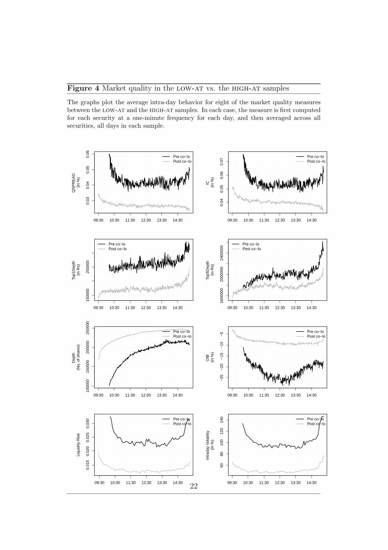
Figure 4 Market quality in the low-at vs. the high-at samples

The graphs plot the average intra-day behavior for eight of the market quality measuresbetween the low-at and the high-at samples. In each case, the measure is first computedfor each security at a one-minute frequency for each day, and then averaged across allsecurities, all days in each sample.

09:30 10:30 11:30 12:30 13:30 14:30

0.03

0.04

0.05

0.06

QS

PR

EA

D

(in %

)

Pre co−loPost co−lo

09:30 10:30 11:30 12:30 13:30 14:300.

040.

050.

060.

07

IC

(in %

)

Pre co−loPost co−lo

09:30 10:30 11:30 12:30 13:30 14:30

1500

0025

0000

Top1

Dep

th

(in R

s)

Pre co−loPost co−lo

09:30 10:30 11:30 12:30 13:30 14:30

1600

000

2000

000

2400

000

Top5

Dep

th

(in R

s)

Pre co−loPost co−lo

09:30 10:30 11:30 12:30 13:30 14:30

1000

0015

0000

2000

0025

0000

Dep

th

(No.

of s

hare

s)

Pre co−loPost co−lo

09:30 10:30 11:30 12:30 13:30 14:30

−25

−20

−15

−10

−5

OIB

(in

%)

Pre co−loPost co−lo

09:30 10:30 11:30 12:30 13:30 14:30

0.01

50.

020

0.02

50.

030

Liqu

idity

Ris

k

Pre co−loPost co−lo

09:30 10:30 11:30 12:30 13:30 14:30

6080

100

120

140

Intr

aday

Vol

atili

ty

(in %

)

Pre co−loPost co−lo

22

Table 4 Summary statistics of the data

The table presents summary statistics of market quality variable for the one month low-at and high-at samples.at-intensity is measured as the percentage of total traded value in which an AT waspresent at either one side or both sides of the trade.qspread is the bid-ask spread as a percentage of mid-quote prices. ic denotes the impactcost computed at a transaction size of Rs. 25,000 (USD 416). top1depth shows the Rupeedepth at the best bid and ask prices, while top5depth shows the cumulated Rupee depthat the top five prices. oib is the order imbalance measured as the difference between thetotal outstanding buy side and sell side shares, and expressed as a percentage of averagetotal depth. σic is the variance of impact cost. rvol is the 5-minutes variance of returnsof each security. vr is the variance ratio computed as the ratio of ten minutes returns tofive minute returns.Values marked with ∗∗ show the values in the high-at sample which are significantlydifferent from low-at values at 0.05%.

low-at high-atMean SD Median Mean SD Median

at-intensity (in %) 13.59 7.58 11.04 54.42∗∗ 10.69 55.57

Transactions costsqspread (in %) 0.05 0.01 0.05 0.03∗∗ 0.01 0.03IC (in %) 0.07 0.02 0.06 0.04∗∗ 0.01 0.04

Depthtop1depth (Rs) 619,873 259,074 272,130 267,791∗∗ 96,428 176,837top5depth (Rs) 2,850,356 983,148 2,077,488 2,034,486∗∗ 579,302 1836,980

depth (No. of shares) 185,447 55,553 194,554 230,949 33,258 239,661oib (in %) -17.14 34.95 -18.66 -8.97∗∗ 15.87 -9.26

Risk, annualised (in %)rvol 102.02 13.50 96.83 51.56∗∗ 5.71 49.82lrisk 69.99 15.63 55.25 37.44∗∗ 6.18 33.67

EfficiencyVR (At k=2) 0.96 0.06 0.96 0.94 0.06 0.92

23

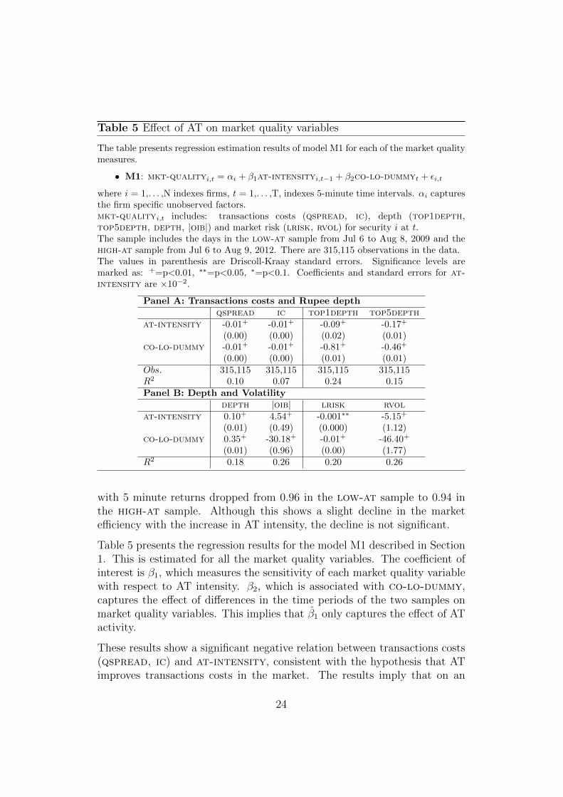
Table 5 Effect of AT on market quality variables

The table presents regression estimation results of model M1 for each of the market qualitymeasures.

• M1: mkt-qualityi,t = αi + β1at-intensityi,t−1 + β2co-lo-dummyt + εi,t

where i = 1,. . . ,N indexes firms, t = 1,. . . ,T, indexes 5-minute time intervals. αi capturesthe firm specific unobserved factors.mkt-qualityi,t includes: transactions costs (qspread, ic), depth (top1depth,top5depth, depth, |oib|) and market risk (lrisk, rvol) for security i at t.The sample includes the days in the low-at sample from Jul 6 to Aug 8, 2009 and thehigh-at sample from Jul 6 to Aug 9, 2012. There are 315,115 observations in the data.The values in parenthesis are Driscoll-Kraay standard errors. Significance levels aremarked as: +=p<0.01, ∗∗=p<0.05, ∗=p<0.1. Coefficients and standard errors for at-intensity are ×10−2.

Panel A: Transactions costs and Rupee depthqspread ic top1depth top5depth

at-intensity -0.01+ -0.01+ -0.09+ -0.17+

(0.00) (0.00) (0.02) (0.01)co-lo-dummy -0.01+ -0.01+ -0.81+ -0.46+

(0.00) (0.00) (0.01) (0.01)Obs. 315,115 315,115 315,115 315,115R2 0.10 0.07 0.24 0.15Panel B: Depth and Volatility

depth |oib| lrisk rvolat-intensity 0.10+ 4.54+ -0.001∗∗ -5.15+

(0.01) (0.49) (0.000) (1.12)co-lo-dummy 0.35+ -30.18+ -0.01+ -46.40+

(0.01) (0.96) (0.00) (1.77)R2 0.18 0.26 0.20 0.26

with 5 minute returns dropped from 0.96 in the low-at sample to 0.94 inthe high-at sample. Although this shows a slight decline in the marketefficiency with the increase in AT intensity, the decline is not significant.

Table 5 presents the regression results for the model M1 described in Section1. This is estimated for all the market quality variables. The coefficient ofinterest is β1, which measures the sensitivity of each market quality variablewith respect to AT intensity. β2, which is associated with co-lo-dummy,captures the effect of differences in the time periods of the two samples onmarket quality variables. This implies that β̂1 only captures the effect of ATactivity.

These results show a significant negative relation between transactions costs(qspread, ic) and at-intensity, consistent with the hypothesis that ATimproves transactions costs in the market. The results imply that on an

24

average, a 1% increase in at-intensity reduces qspread and ic by 1 bps.

The total depth (measured as the number of shares) is also positively im-pacted by at-intensity. A 1% increase in at-intensity intensity increasesdepth by 0.10%. The improvement in transactions costs and total depth ishowever not matched with an increase in the Rupee depth in the markets.We see that a 1% increase in at-intensity brings about a 0.09% declinein Rupee depth at best prices, and 0.17% decline at the top five prices, onaverage. This is contrary to the expectation that AT provides additional liq-uidity. The coefficient associated with |oib| also shows an adverse impact ofAT on oib. We see that a 1% increase in AT can bring about 4.54% wideningin order imbalance on the limit order books.

Both risk measures – lrisk as well as rvol – showed a significant declineas a result of AT activity. Higher levels of AT activity are associated withlower levels of liquidity risk.

Overall the results suggest that AT has a positive improvement market qual-ity by way of reduction in transactions costs and reduction in the risks ofthe security. We also see an improvement in the total depth. But we donot see a corresponding increase in Rupee depth or an improvement in orderimbalance. This result is similar to Hendershott et al. (2011) who also finda decline in quoted depth after the introduction of co-lo.

7.2 Threats to validity: Did other factors cause thechange in market quality?

The results in Section 7.1 show that, around the period of the introduction ofco-lo and the subsequent increase of AT intensity, market quality has tendedto improve. Transactions costs, securities volatility and liquidity risk haveall reduced while total depth has increased as a consequence of AT. On theother hand, the Rupee depth has decreased, and the gap between the buyand the sell side has widened.

However, security liquidity and volatility can be affected by other factorssuch as macro-economic shocks like the global crisis of 2008, that increasemarket volatility and liquidity. In that case, could these results be attributedto the increase in AT after co-lo, or were they instead caused reduced marketvolatility and reduced market price levels (which is the case in the high-atsample)?

We address such questions using the two approaches described in Section 5.3.

25

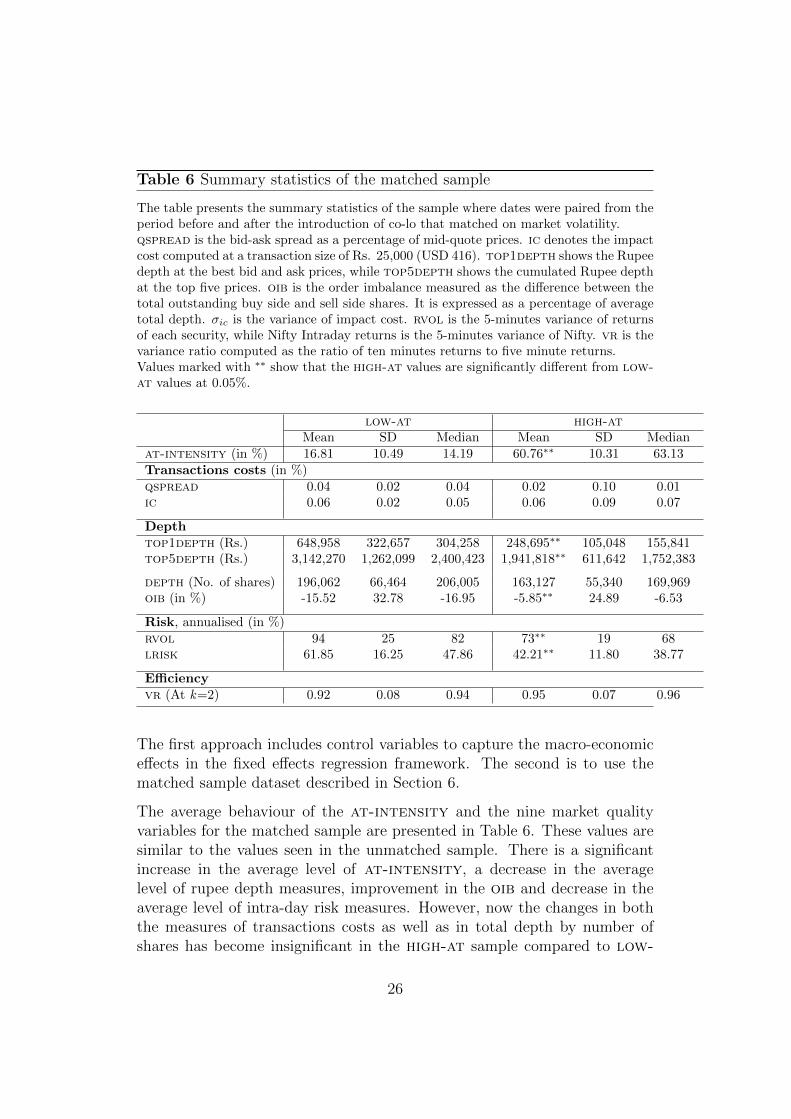
Table 6 Summary statistics of the matched sample

The table presents the summary statistics of the sample where dates were paired from theperiod before and after the introduction of co-lo that matched on market volatility.qspread is the bid-ask spread as a percentage of mid-quote prices. ic denotes the impactcost computed at a transaction size of Rs. 25,000 (USD 416). top1depth shows the Rupeedepth at the best bid and ask prices, while top5depth shows the cumulated Rupee depthat the top five prices. oib is the order imbalance measured as the difference between thetotal outstanding buy side and sell side shares. It is expressed as a percentage of averagetotal depth. σic is the variance of impact cost. rvol is the 5-minutes variance of returnsof each security, while Nifty Intraday returns is the 5-minutes variance of Nifty. vr is thevariance ratio computed as the ratio of ten minutes returns to five minute returns.Values marked with ∗∗ show that the high-at values are significantly different from low-at values at 0.05%.

low-at high-atMean SD Median Mean SD Median

at-intensity (in %) 16.81 10.49 14.19 60.76∗∗ 10.31 63.13Transactions costs (in %)qspread 0.04 0.02 0.04 0.02 0.10 0.01ic 0.06 0.02 0.05 0.06 0.09 0.07

Depthtop1depth (Rs.) 648,958 322,657 304,258 248,695∗∗ 105,048 155,841top5depth (Rs.) 3,142,270 1,262,099 2,400,423 1,941,818∗∗ 611,642 1,752,383

depth (No. of shares) 196,062 66,464 206,005 163,127 55,340 169,969oib (in %) -15.52 32.78 -16.95 -5.85∗∗ 24.89 -6.53

Risk, annualised (in %)rvol 94 25 82 73∗∗ 19 68lrisk 61.85 16.25 47.86 42.21∗∗ 11.80 38.77

Efficiencyvr (At k=2) 0.92 0.08 0.94 0.95 0.07 0.96

The first approach includes control variables to capture the macro-economiceffects in the fixed effects regression framework. The second is to use thematched sample dataset described in Section 6.

The average behaviour of the at-intensity and the nine market qualityvariables for the matched sample are presented in Table 6. These values aresimilar to the values seen in the unmatched sample. There is a significantincrease in the average level of at-intensity, a decrease in the averagelevel of rupee depth measures, improvement in the oib and decrease in theaverage level of intra-day risk measures. However, now the changes in boththe measures of transactions costs as well as in total depth by number ofshares has become insignificant in the high-at sample compared to low-

26

at. This suggests that the some of the improvements in average levels ofliquidity seen in Table 4 might have been influenced by the market volatility,rather than the change in average at-intensity in the market.

Next, we present the estimations of the regression framework with controlvariables added to capture the macroeconomic factors that can influencemarket quality. These lead to the three models – M2, M3, M4 – that aredescribed in Section 5.3. The estimates for each of these models for all thenine market quality variables are presented in Appendix A.

Our focus is only on the estimates for the coefficient of at-intensity, β̂1.We ask whether the coefficient value presented in Table 5 has a differentmagnitude or significance when estimated with controls for macroeconomicfactors such as market volatility, or using the matched sample.

Table 7 presents the following four sets of estimates of β1: (1) M1 which doesnot control for macroeconomic factors and other factors (such as the priceof the security, intraday effects); (2) M4, which controls for macroeconomicfactors; (3) M1’ which is estimated using the matched sample, but withoutany controls for macroeconomic factors; and (4) M4’ which is estimatedusing the matched sample and also includes controls for macroeconomic andother factors. The estimated β̂1 is presented for each market quality variable.

The table shows that the results of lower transactions costs – whether forqspread or ic – holds across all the specification. This is also true for thedepth that is available at the best price (top1depth) and across the bestfive prices (top1depth) in the limit order book. For these four measures ofliquidity, these results suggest that AT has improved market quality.

The results also appear to be consistent across all specifications for the twomeasures of market risk. Intraday price volatility (rvol) has dropped asa consequence of AT. The magnitude of the drop in rvol is higher whenthe estimations use the matched sample, where market volatility is the samefor paired dates in the low-at and high-at samples. This result suggestsa stronger result about the impact of AT on intraday volatility comparedto what the one-month low-at and high-at samples suggested. Intradayliquidity risk, lrisk is consistently lower when AT is higher with a negativevalue of β̂1, but the result is weaker than those for intraday price volatility.

In all the above variabels, we infer that AT has improved market quality.

For two of the market quality variables, the results indicate that higher ATleads to poorer market quality. In the case of the difference in the numberof shares available on the buy and sell side of the limit order book, oib,

27

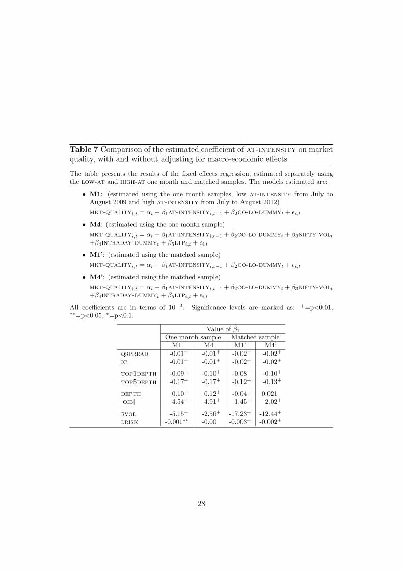
Table 7 Comparison of the estimated coefficient of at-intensity on marketquality, with and without adjusting for macro-economic effects

The table presents the results of the fixed effects regression, estimated separately usingthe low-at and high-at one month and matched samples. The models estimated are:

• M1: (estimated using the one month samples, low at-intensity from July toAugust 2009 and high at-intensity from July to August 2012)

mkt-qualityi,t = αi + β1at-intensityi,t−1 + β2co-lo-dummyt + εi,t

• M4: (estimated using the one month sample)

mkt-qualityi,t = αi + β1at-intensityi,t−1 + β2co-lo-dummyt + β3nifty-volt+β4intraday-dummyt + β5ltpi,t + εi,t

• M1’: (estimated using the matched sample)

mkt-qualityi,t = αi + β1at-intensityi,t−1 + β2co-lo-dummyt + εi,t

• M4’: (estimated using the matched sample)

mkt-qualityi,t = αi + β1at-intensityi,t−1 + β2co-lo-dummyt + β3nifty-volt+β4intraday-dummyt + β5ltpi,t + εi,t

All coefficients are in terms of 10−2. Significance levels are marked as: +=p<0.01,∗∗=p<0.05, ∗=p<0.1.

Value of β̂1One month sample Matched sample

M1 M4 M1’ M4’qspread -0.01+ -0.01+ -0.02+ -0.02+

ic -0.01+ -0.01+ -0.02+ -0.02+

top1depth -0.09+ -0.10+ -0.08+ -0.10+

top5depth -0.17+ -0.17+ -0.12+ -0.13+

depth 0.10+ 0.12+ -0.04+ 0.021|oib| 4.54+ 4.91+ 1.45+ 2.02+

rvol -5.15+ -2.56+ -17.23+ -12.44+

lrisk -0.001∗∗ -0.00 -0.003+ -0.002+

28

higher AT leads to a wider gap between the two. These results are consistentacross all the models estimated. When the estimated is based on the matchedsample, the increase in the gap is smaller.

It is only in the case of depth that the results are inconsistent between theestimation uses the one-month low-at and high-at samples compared tothe matched samples. β̂1 when estimations use the matched sample eithergive a negative value (while the remaining estimates are positive) or an in-significant value. While the results corroborate the findings of Hendershottet al. (2011), it needs to be further investigated as to what leads a decline indepth of the markets as a result of high at-intensity.

Thus, other than for two of the market quality variables, the results show thathigher AT leads to improvements in market quality, and that these resultsare robust even when the estimations adjust for macroeconomic factors.

8 Conclusion

There is a rapidly growing literature on how the presence of algorithmictrading (AT) has changed the liquidity and volatility of markets. This ispartly fueled by the regulatory concerns that the use of technology skews theaccess to markets to a small fraction of the trading community. But, anotherpart of the continuing quest for an answer to this question is founded in thelack of clear identification of whether the orders and trades originate froman AT source or not. While there are some papers that have access to suchdetails from exchanges, the datasets are too small and not comprehensiveenough to yield general results. The larger fraction of research is based onproxy measures of AT, which raises questions about the validity of the results.

In this paper, we use access to data from the equity markets of the NationalStock Exchange (NSE), where every order is tagged by as AT or non-AT.Unlike in other markets, all equity trading is pooled in two exchanges andthe NSE has around 70 percent of the marketshare. Further, the span of thisdata includes the date when the NSE introduced co-location (co-lo) facilities,which serves to identify a specific date beyond which AT intensity was boundto increase in the market. Therefore, this study helps to address concernsabout the lack of generality of previous studies. We use the direct identi-fication of the orders as AT to calculate the at-intensity in the marketany given point in time. We find that the at-intensity did go up after theintroduction of co-lo services, but did not stabilise immediately.

29

We measure the impact of AT on both the average, or overall market quality,as well as in a cross-sectional analysis. Since the span of the analysis coversa wide period, we control for changes in exogenous factors (such as marketvolatility) that as likely as higher levels of at-intensity to cause the changesobserved in market quality. We also repeat the comparative analysis on theaverage and the cross-sectional variation using matched low-at and high-at samples, where dates are selected that are matched on the level of marketvolatility.

Both approaches indicate that transactions costs have decreased with higherlevels of AT, but that market depth has decreased. The decrease in depthholds for depth measured as total value (in Rupees) available for trade atthe touch and at the best five prices available in the limit order book. Thisresult also holds for the overall market depth (in number of shares). Theseresults about lowered costs and worsened depth with higher at-intensityare similar to those Hendershott et al. (2011). The results about intradayprice volatility of prices is similar to much of the empirical literature (Has-brouck and Saar, 2013; Brogaard, 2010). We also test the behaviour of thevolatility of transactions costs, and find that liquidity risk has decreased withthe rise in at-intensity. This runs counter to popular arguments that therise of algorithmic trading has increased liquidity risk in the market. Finally,we analyse the impact of AT on market efficiency as measured by the vari-ance ratio, and find no significant changes in the intra-day behaviour of thevariance ratio because of higher at-intensity.

Thus, the results in the paper mostly validates the findings in the literatureabout how algorithmic trading affects transactions costs and depth. It addsto the understanding about market volatility by showing that higher at-intensity significantly improves (has a negative effect) on both intra-dayprice volatility as well as liquidity risk. Given the clear identification, thecomprehensive cover and the span of the data used in the analysis, theseresults should help address the concerns about the lack of generality of someof the earlier empirical analysis in the literature.

What this work also does is to highlights several new aspects of the impactof AT on the market quality of securities that require further research. Oneobservation that emerges from the analysis is that there is a wide degree ofheterogeneity of at-intensity across securities. In the Indian equity mar-ket, where there was a clear event that facilitated AT into the market atthe same time, where all trading is pooled into two exchanges with no otherdark pools or other avenues of trading available, the question arises as to towhy certain securities attract more AT focus than others. Are the selections

30

temporary patterns, driven by the arrival of news, either about the companyitself, or the overall market environment? Or are these more structural rea-sons for these choices, driven by differences in information asymmetry acrossdifferent companies that are related to differences in corporate disclosurequality? Given the benefits that accrue to the market quality of securitiesthat have a high degree of AT intensity, these are interesting questions forboth investors as well as issuers of securities.

31

A Estimations addressing threats to validity

32

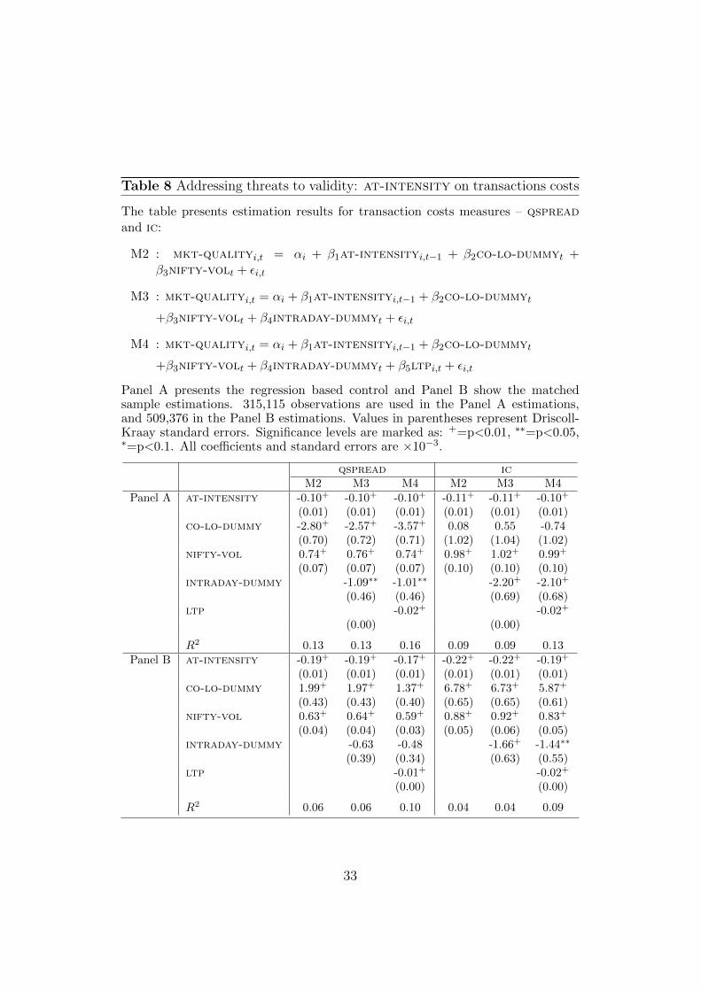
Table 8 Addressing threats to validity: at-intensity on transactions costs

The table presents estimation results for transaction costs measures – qspreadand ic:

M2 : mkt-qualityi,t = αi + β1at-intensityi,t−1 + β2co-lo-dummyt +β3nifty-volt + εi,t

M3 : mkt-qualityi,t = αi + β1at-intensityi,t−1 + β2co-lo-dummyt

+β3nifty-volt + β4intraday-dummyt + εi,t

M4 : mkt-qualityi,t = αi + β1at-intensityi,t−1 + β2co-lo-dummyt

+β3nifty-volt + β4intraday-dummyt + β5ltpi,t + εi,t

Panel A presents the regression based control and Panel B show the matchedsample estimations. 315,115 observations are used in the Panel A estimations,and 509,376 in the Panel B estimations. Values in parentheses represent Driscoll-Kraay standard errors. Significance levels are marked as: +=p<0.01, ∗∗=p<0.05,∗=p<0.1. All coefficients and standard errors are ×10−3.

qspread icM2 M3 M4 M2 M3 M4

Panel A at-intensity -0.10+ -0.10+ -0.10+ -0.11+ -0.11+ -0.10+

(0.01) (0.01) (0.01) (0.01) (0.01) (0.01)co-lo-dummy -2.80+ -2.57+ -3.57+ 0.08 0.55 -0.74

(0.70) (0.72) (0.71) (1.02) (1.04) (1.02)nifty-vol 0.74+ 0.76+ 0.74+ 0.98+ 1.02+ 0.99+

(0.07) (0.07) (0.07) (0.10) (0.10) (0.10)intraday-dummy -1.09∗∗ -1.01∗∗ -2.20+ -2.10+

(0.46) (0.46) (0.69) (0.68)ltp -0.02+ -0.02+

(0.00) (0.00)

R2 0.13 0.13 0.16 0.09 0.09 0.13Panel B at-intensity -0.19+ -0.19+ -0.17+ -0.22+ -0.22+ -0.19+

(0.01) (0.01) (0.01) (0.01) (0.01) (0.01)co-lo-dummy 1.99+ 1.97+ 1.37+ 6.78+ 6.73+ 5.87+

(0.43) (0.43) (0.40) (0.65) (0.65) (0.61)nifty-vol 0.63+ 0.64+ 0.59+ 0.88+ 0.92+ 0.83+

(0.04) (0.04) (0.03) (0.05) (0.06) (0.05)intraday-dummy -0.63 -0.48 -1.66+ -1.44∗∗

(0.39) (0.34) (0.63) (0.55)ltp -0.01+ -0.02+

(0.00) (0.00)

R2 0.06 0.06 0.10 0.04 0.04 0.09

33

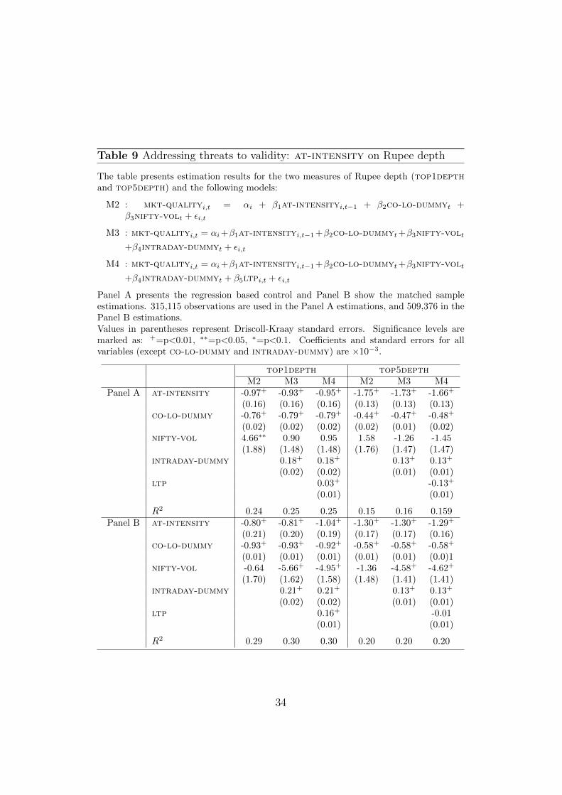
Table 9 Addressing threats to validity: at-intensity on Rupee depth

The table presents estimation results for the two measures of Rupee depth (top1depthand top5depth) and the following models:

M2 : mkt-qualityi,t = αi + β1at-intensityi,t−1 + β2co-lo-dummyt +β3nifty-volt + εi,t

M3 : mkt-qualityi,t = αi+β1at-intensityi,t−1+β2co-lo-dummyt+β3nifty-volt

+β4intraday-dummyt + εi,t

M4 : mkt-qualityi,t = αi+β1at-intensityi,t−1+β2co-lo-dummyt+β3nifty-volt

+β4intraday-dummyt + β5ltpi,t + εi,t

Panel A presents the regression based control and Panel B show the matched sampleestimations. 315,115 observations are used in the Panel A estimations, and 509,376 in thePanel B estimations.Values in parentheses represent Driscoll-Kraay standard errors. Significance levels aremarked as: +=p<0.01, ∗∗=p<0.05, ∗=p<0.1. Coefficients and standard errors for allvariables (except co-lo-dummy and intraday-dummy) are ×10−3.

top1depth top5depthM2 M3 M4 M2 M3 M4

Panel A at-intensity -0.97+ -0.93+ -0.95+ -1.75+ -1.73+ -1.66+

(0.16) (0.16) (0.16) (0.13) (0.13) (0.13)co-lo-dummy -0.76+ -0.79+ -0.79+ -0.44+ -0.47+ -0.48+

(0.02) (0.02) (0.02) (0.02) (0.01) (0.02)nifty-vol 4.66∗∗ 0.90 0.95 1.58 -1.26 -1.45

(1.88) (1.48) (1.48) (1.76) (1.47) (1.47)intraday-dummy 0.18+ 0.18+ 0.13+ 0.13+

(0.02) (0.02) (0.01) (0.01)ltp 0.03+ -0.13+

(0.01) (0.01)

R2 0.24 0.25 0.25 0.15 0.16 0.159Panel B at-intensity -0.80+ -0.81+ -1.04+ -1.30+ -1.30+ -1.29+

(0.21) (0.20) (0.19) (0.17) (0.17) (0.16)co-lo-dummy -0.93+ -0.93+ -0.92+ -0.58+ -0.58+ -0.58+

(0.01) (0.01) (0.01) (0.01) (0.01) (0.0)1nifty-vol -0.64 -5.66+ -4.95+ -1.36 -4.58+ -4.62+

(1.70) (1.62) (1.58) (1.48) (1.41) (1.41)intraday-dummy 0.21+ 0.21+ 0.13+ 0.13+

(0.02) (0.02) (0.01) (0.01)ltp 0.16+ -0.01

(0.01) (0.01)

R2 0.29 0.30 0.30 0.20 0.20 0.20

34

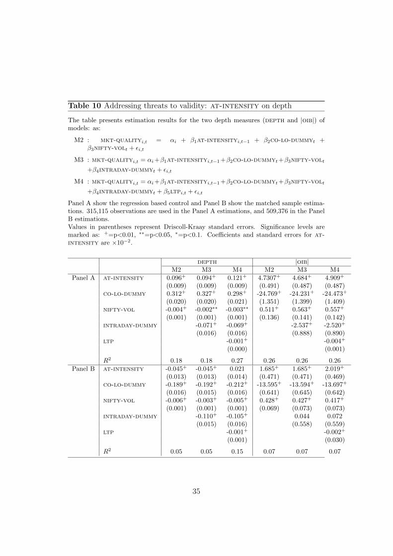
Table 10 Addressing threats to validity: at-intensity on depth

The table presents estimation results for the two depth measures (depth and |oib|) ofmodels: as:

M2 : mkt-qualityi,t = αi + β1at-intensityi,t−1 + β2co-lo-dummyt +β3nifty-volt + εi,t

M3 : mkt-qualityi,t = αi+β1at-intensityi,t−1+β2co-lo-dummyt+β3nifty-volt

+β4intraday-dummyt + εi,t

M4 : mkt-qualityi,t = αi+β1at-intensityi,t−1+β2co-lo-dummyt+β3nifty-volt

+β4intraday-dummyt + β5ltpi,t + εi,t

Panel A show the regression based control and Panel B show the matched sample estima-tions. 315,115 observations are used in the Panel A estimations, and 509,376 in the PanelB estimations.Values in parentheses represent Driscoll-Kraay standard errors. Significance levels aremarked as: +=p<0.01, ∗∗=p<0.05, ∗=p<0.1. Coefficients and standard errors for at-intensity are ×10−2.

depth |oib|M2 M3 M4 M2 M3 M4

Panel A at-intensity 0.096+ 0.094+ 0.121+ 4.7307+ 4.684+ 4.909+

(0.009) (0.009) (0.009) (0.491) (0.487) (0.487)co-lo-dummy 0.312+ 0.327+ 0.298+ -24.769+ -24.231+ -24.473+

(0.020) (0.020) (0.021) (1.351) (1.399) (1.409)nifty-vol -0.004+ -0.002∗∗ -0.003∗∗ 0.511+ 0.563+ 0.557+

(0.001) (0.001) (0.001) (0.136) (0.141) (0.142)intraday-dummy -0.071+ -0.069+ -2.537+ -2.520+

(0.016) (0.016) (0.888) (0.890)ltp -0.001+ -0.004+

(0.000) (0.001)

R2 0.18 0.18 0.27 0.26 0.26 0.26Panel B at-intensity -0.045+ -0.045+ 0.021 1.685+ 1.685+ 2.019+

(0.013) (0.013) (0.014) (0.471) (0.471) (0.469)co-lo-dummy -0.189+ -0.192+ -0.212+ -13.595+ -13.594+ -13.697+

(0.016) (0.015) (0.016) (0.641) (0.645) (0.642)nifty-vol -0.006+ -0.003+ -0.005+ 0.428+ 0.427+ 0.417+

(0.001) (0.001) (0.001) (0.069) (0.073) (0.073)intraday-dummy -0.110+ -0.105+ 0.044 0.072

(0.015) (0.016) (0.558) (0.559)ltp -0.001+ -0.002+

(0.001) (0.030)

R2 0.05 0.05 0.15 0.07 0.07 0.07

35

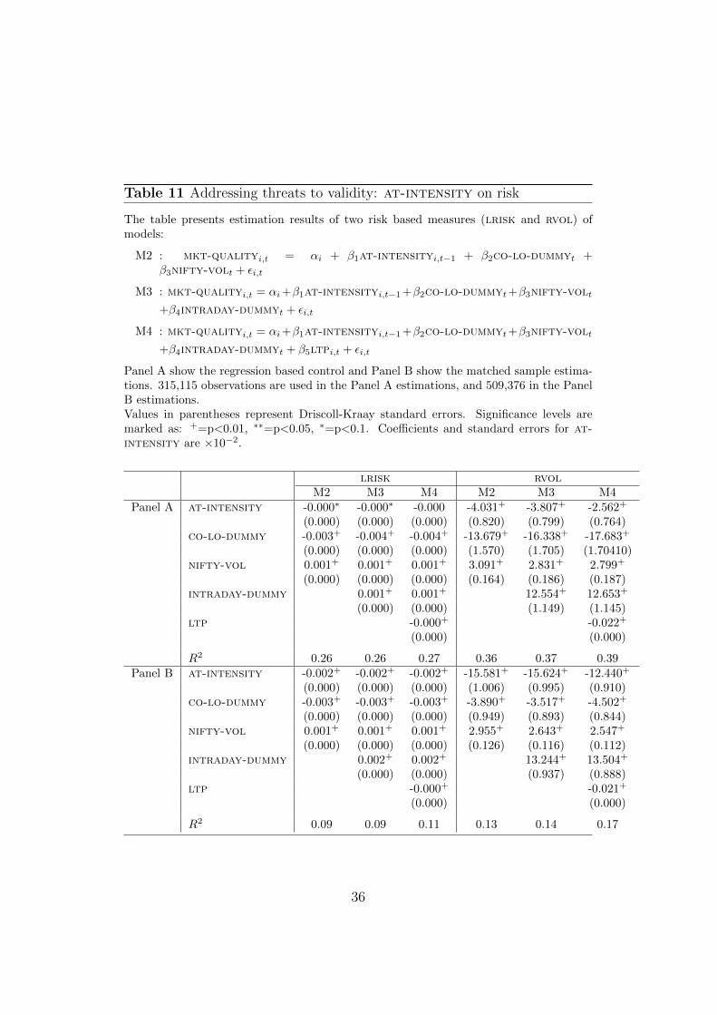
Table 11 Addressing threats to validity: at-intensity on risk

The table presents estimation results of two risk based measures (lrisk and rvol) ofmodels:

M2 : mkt-qualityi,t = αi + β1at-intensityi,t−1 + β2co-lo-dummyt +β3nifty-volt + εi,t

M3 : mkt-qualityi,t = αi+β1at-intensityi,t−1+β2co-lo-dummyt+β3nifty-volt

+β4intraday-dummyt + εi,t

M4 : mkt-qualityi,t = αi+β1at-intensityi,t−1+β2co-lo-dummyt+β3nifty-volt

+β4intraday-dummyt + β5ltpi,t + εi,t

Panel A show the regression based control and Panel B show the matched sample estima-tions. 315,115 observations are used in the Panel A estimations, and 509,376 in the PanelB estimations.Values in parentheses represent Driscoll-Kraay standard errors. Significance levels aremarked as: +=p<0.01, ∗∗=p<0.05, ∗=p<0.1. Coefficients and standard errors for at-intensity are ×10−2.

lrisk rvolM2 M3 M4 M2 M3 M4

Panel A at-intensity -0.000∗ -0.000∗ -0.000 -4.031+ -3.807+ -2.562+

(0.000) (0.000) (0.000) (0.820) (0.799) (0.764)co-lo-dummy -0.003+ -0.004+ -0.004+ -13.679+ -16.338+ -17.683+

(0.000) (0.000) (0.000) (1.570) (1.705) (1.70410)nifty-vol 0.001+ 0.001+ 0.001+ 3.091+ 2.831+ 2.799+

(0.000) (0.000) (0.000) (0.164) (0.186) (0.187)intraday-dummy 0.001+ 0.001+ 12.554+ 12.653+

(0.000) (0.000) (1.149) (1.145)ltp -0.000+ -0.022+

(0.000) (0.000)

R2 0.26 0.26 0.27 0.36 0.37 0.39Panel B at-intensity -0.002+ -0.002+ -0.002+ -15.581+ -15.624+ -12.440+

(0.000) (0.000) (0.000) (1.006) (0.995) (0.910)co-lo-dummy -0.003+ -0.003+ -0.003+ -3.890+ -3.517+ -4.502+

(0.000) (0.000) (0.000) (0.949) (0.893) (0.844)nifty-vol 0.001+ 0.001+ 0.001+ 2.955+ 2.643+ 2.547+

(0.000) (0.000) (0.000) (0.126) (0.116) (0.112)intraday-dummy 0.002+ 0.002+ 13.244+ 13.504+

(0.000) (0.000) (0.937) (0.888)ltp -0.000+ -0.021+

(0.000) (0.000)

R2 0.09 0.09 0.11 0.13 0.14 0.17

36

References

Biais B, Foucault T, Moinas S (2013). “Equilibrium Fast Trading.” Workingpaper. URL http://papers.ssrn.com/sol3/papers.cfm?abstract_id=

1859265.

Bohemer E, Fong K, Wu J (2012). “International Evidence on Algorith-mic Trading.” Working Paper. URL http://papers.ssrn.com/sol3/

papers.cfm?abstract_id=2022034.

Brogaard J (2010). “High Frequency Trading and Its Impact on Market Qual-ity.” Working Paper. URL www.futuresindustry.org/ptg/downloads/

HFT_Trading.pdf.

Brogaard J, Hendershott T, Riordan R (2012). “High frequency trading andprice discovery.” Working Paper, University of California at Berkeley.

Carrion A (2013). “Very fast money: High-frequency trading on the{NASDAQ}.” Journal of Financial Markets, 16(4), 680 – 711.

Cartea A, Penalva J (2012). “Where is the Value in High Frequency Trad-ing?” Quarterly Journal of Finance, 02(03), 1250014.

Chaboud A, Chiquoine B, Hjalmarsson E, Vega C (2009). “Rise of themachines: algorithmic trading in the foreign exchange market.” URLhttp://ideas.repec.org/p/fip/fedgif/980.html.

Chordia T, Roll R, Subrahmanyam A (2000). “Commonality in liquidity.”Journal of Financial Economics, 56(1), 3 – 28.

Driscoll JC, Kraay AC (1998). “Consistent Covariance Matrix EstimationWith Spatially Dependent Panel Data.” The Review of Economics andStatistics, 80(4), 549–560.

Foucault T (1999). “Order flow composition and trading costs in a dynamiclimit order market.” Journal of Financial Markets, 2(2), 99 – 134.

Frino A, Mollica V, Webb RI (2013). “The impact of co-location of securitiesexchanges’ and traders’ computer servers on market liquidity.” Journal ofFutures Markets. ISSN 1096-9934.

Grossman SJ, Miller MH (1988). “Liquidity and Market Structure.” TheJournal of Finance, 43(3), 617–633.

37

Hameed A, Kang W, Vishwanathan S (2010). “Stock Market Declines andLiquidity.” The Journal of Finance, 65(1), 257–293.

Hasbrouck J, Saar G (2013). “Low-latency trading.” Journal of FinancialMarkets, 16(4), 646 – 679.

Hendershott T, Jones CM, Menkveld AJ (2011). “Does Algorithmic TradingImprove Liquidity?” The Journal of Finance, 66(1), 1–33.

Hendershott T, Riordan R (2013). “Algorithmic trading and the market forliquidity.” The Journal of Financial and Quantitative Analysis, Forthcom-ing.

Hoffmann P (2012). “A dynamic limit order market with fast and slowtraders.” Technical report, University Library of Munich, Germany. URLhttp://ideas.repec.org/p/pra/mprapa/39855.html.

Jovanovic B, Menkveld AJ (2010). “Middlemen in Limit Order Mar-kets.” 2010 meeting papers, Society for Economic Dynamics. URLhttp://ideas.repec.org/p/red/sed010/955.html.

Lo A, MacKinlay A (1988). “Stock market prices do not follow random walks:evidence from a simple specification test.” Review of Financial Studies,1(1), 41–66.

Martinez VH, Rosu I (2013). “High-frequency traders, news and volatil-ity.” Working paper. URL http://papers.ssrn.com/sol3/papers.cfm?

abstract_id=1859265.

Menkveld AJ (2013). “High frequency trading and the new market mak-ers.” Journal of Financial Markets, 16(4), 712 – 740. URL http://www.

sciencedirect.com/science/article/pii/S1386418113000281.

Moura M, Pereira F, Attuy G (2013). “Currency Wars in Action:How Foreign Exchange Interventions Work in an Emerging Economy.”(304/2013). URL http://www.insper.edu.br/wp-content/uploads/

2013/06/2013_wpe304.pdf.

Riordan R, Storkenmaier A (2012). “Latency, liquidity and price discovery.”Journal of Financial Markets, 15(4), 416 – 437.

SEBI (2013). “Table 2: The Basic Indicators in Cash Market.” SEBI Bul-letin, November 2013, www.sebi.gov.in/cms/sebi_data/attachdocs/

1385638179478.pdf.

38

Thomas S (2010). “Call auctions: A solution to some difficulties in In-dian finance.” Working Paper. URL http://www.igidr.ac.in/pdf/

publication/WP-2010-006.pdf.

Viljoen T, Zheng H, Westerholm PJ (2011). “Liquidity and Price Discovery ofAlgorithmic Trading: An Intraday Analysis of the SPI 200 Futures.” URLhttp://papers.ssrn.com/sol3/papers.cfm?abstract_id=1913693.

Zhang F (2010). “High-Frequency Trading, Stock Volatility, and Price Dis-covery.” URL http://papers.ssrn.com/sol3/papers.cfm?abstract_

id=1691679.

39