market madness? the case of mad money*
TRANSCRIPT

Market Madness? The Case of Mad Money*
Joseph Engelberg
Caroline Sasseville
Jared Williams‡
October 2010
Abstract: We use the popular television show Mad Money hosted by Jim Cramer to test theories of attention and limits to arbitrage. Stock recommendations on Mad Money constitute attention shocks to a large audience of individual traders. We find that stock recommendations lead to large overnight returns which subsequently reverse over the next few months. The spike-reversal pattern is strongest among small, illiquid stocks that are hard-to-arbitrage. Using daily Nielsen ratings as a direct measure of attention, we find the overnight return is strongest when high income viewership is high. We also find weak price effects among sell recommendations. Taken together, the evidence supports the retail attention hypothesis of Barber and Odean (2008) and illustrates the potential role of media in generating mispricing.
*We thank Brad Barber (the editor), the associate editor, and two anonymous referees for their suggestions. We have also benefited from discussions with Flavio de Andrade, Nick Barberis, Fritz Burkhardt, Jennifer Conrad, Grant Farnsworth, Paul Gao, Dave Haushalter, Zhiguo He, Andrew Hertzberg, Ravi Jagannathan, Pab Jotikasthira, David Matsa, Adam Reed, Ed Van Wesep, and Annette Vissing-Jorgensen. ‡ Contact: Joseph Engelberg, Kenan-Flagler Business School, University of North Carolina at Chapel Hill, (Email) [email protected]; Caroline Sasseville, Barclays Global Investors; and Jared Williams, Smeal College of Business, Penn State University, 344 Business Building (Email) [email protected].

2
I. Introduction
Financial economists have become increasingly interested in the relationship between
attention and asset prices. This interest is motivated by examples of large changes in equity prices
that appear to be driven by attention alone. For example, Huberman and Regev (2001) document the
case of cancer drug company EntreMed whose stock price tripled based on a favorable front-page
article in the New York Times in May of 1998 even though all the information in the article had been
released twelve months earlier in the journal Nature. Retail investors are unlikely to read Nature but
likely to read headline articles in the New York Times. Barber and Odean (2008) argue that such
attention shocks to retail investors cause temporary price pressure since retail buyers are unlikely to
be sellers.
Although anecdotes suggest retail attention can affect returns and there exists a theory to
explain its effect (Barber and Odean [2008]), empiricists face a substantial problem when linking
retail attention to prices: we rarely observe attention directly. This paper, however, considers a
laboratory in which retail traders trade and we can measure their attention directly. We analyze the
market’s reaction to stock recommendations of Jim Cramer, host of the CNBC show Mad Money,
between June 2005 and February 2009.1
We have three main findings. First, equal-weighted portfolios based on Cramer’s
recommendations — but formed before the recommendations are made — have no statistically-
detectable, long-run alpha. Mad Money typically airs at 6 p.m. EST, and portfolios which buy
1 Although our paper is the first to examine the price response to stocks picked on Mad Money, Neumann and Kenny (2007) repeated the analysis that was in an early draft of this paper and included sell recommendations. Also, Keasler and McNeil (2008) analyzed Cramer's recommendations to test whether the market's response to his recommendations is due to information or price pressure. By looking at the spike-reversal pattern and the bid-ask spreads following his recommendations, they conclude that the market's response is due to price pressure rather than new information. Although subsequent papers have confirmed the spike-reversal pattern in returns that we find in this paper, none have considered the role of investor attention (TV viewership), the role of contemporaneous news, the role of arbitrageurs (via short-selling and rebate rates), or the timing of the market's response in the after-hours market that we consider here.

3
recommended stocks at 4 p.m. (more than two hours before they are recommended) perform no
better than the market when held for 50, 150 or 250 trading days (one year).
Second, even though Cramer’s recommendations do not appear informative in the long-run,
there is a strong short-run effect: the average overnight abnormal return following Cramer’s buy
recommendations is 2.4% which corresponds to an average change in market capitalization of $77.1
million.2 Given there is no long-run effect, this implies that the short-run effect must be
temporary. It is. Long portfolios formed the day after Cramer has made his recommendation earn
an annualized alpha of −9.98% at the 50-day horizon, −6.15% at the 150-day horizon and −3.2% at
the 250-day horizon. Among the quintile of stocks that had the highest overnight return, long
portfolios formed the day after Cramer’s recommendation earn an annualized alpha of −29.54% at
the 50-day horizon, −16.66% at the 150-day horizon and −8.91% at the 250-day horizon.
The first two findings provide evidence of media-induced mispricing: stocks recommended
on Mad Money have prices that immediately become too high. The size of the overnight mispricing,
however, should be related to two key factors: (1) the amount of attention paid to a recommendation
and (2) the market frictions that prevent arbitrageurs from correcting the mispricing. Therefore, our
final set of tests considers the cross-section of recommendations and relates the size of the
mispricing to the size of the attention shock and the limits to arbitrage.
First, we show that less prominent buy recommendations on the show have a smaller
overnight response. Stocks recommended during the “lightning round” segment or on Mad Money
shows with many other recommendations have the smallest overnight returns.
Our most direct tests of the attention hypothesis come when we relate viewership to
overnight mispricing. Using proprietary viewership data from Nielsen Media Research, we find a
positive relationship between total viewership and overnight return. A one standard deviation
2 This computation is based on abnormal returns, which are defined as the stock's returned minus it's Fama-French matched portfolio. See Section 2 for more details on the matching methodology.

4
increase in total viewership leads to additional 30 bps in overnight abnormal return. Moreover,
when we divide total viewership by income we find a strong positive relationship between high
income viewership and overnight return, but no relationship between low income viewership and
overnight return. A one standard deviation increase in the number of high income households
watching the show increases abnormal overnight returns by 34 bps while a one standard deviation
increase in poor viewership has no effect. Our results suggest that the link between the exposure of
public information and the market response may be more complex than previously thought. In
particular, the results suggest that who observes an event may be just as important as how many do.
When we consider limits to arbitrage (e.g., Pontiff [1996] and Shleifer and Vishny [1997]), we
find the largest overnight returns in the set of stocks that are hardest to arbitrage: small, illiquid
stocks with high idiosyncratic volatility. Moreover, for a subset of our sample we are able to obtain
short-selling data from a set of securities lenders. Given the fact that the large overnight returns we
observe eventually reverse, an arbitrageur would like to take a short position in the recommended
stocks. Using proprietary lending data we find stocks with short-sale constraints experience the
largest overnight return.
Our final test of the Barber and Odean (2008) attention hypothesis considers sell
recommendations. Barber and Odean (2008) argue that there should be a strong asymmetric effect
with respect to buying and selling following an attention shock. Because retail traders rarely short,
we should see considerably more buying following an attention shock than selling because selling
would require ex-ante ownership whereas buying does not. The predicted asymmetry is precisely
what we find. While first-time buy recommendations have a large overnight return of 2.4%, first-
time sell recommendations have overnight returns that are smaller in magnitude (-0.29%). There is
also no detectable post-recommendation trend in sell-recommendation returns. The evidence
supports the view that an attention shock in the form of a sell recommendation has little effect on
returns, perhaps because retail traders rarely short.

5
Taken together, our findings contribute to several literatures. The first is a growing literature
which considers the relationship between investor attention and prices. While Huberman and Regev
(2001) focus on one stock, Tetlock (2008) considers “repeat news stories” and finds differential
return patterns based on whether news stories are repeated in the media. DellaVigna and Pollet
(2009) find a weaker response to earnings announcements on Fridays when presumably fewer
traders are present. A shortcoming in each of these papers is the identification strategy. Although the
papers infer that asset prices around information events are partially determined by the number of
traders who observe the events, none of these papers can directly measure how many traders observe
the public information. Authors of earlier studies use proxies for this attention, including trading
volume (e.g. Gervais, Kaniel, and Mingelgrin [2001], Barber and Odean [2008], and Hou, Peng, and
Xiong [2008]), the existence of news (Barber and Odean [2008]), firms’ advertising expenses
(Grullon, Kanatas, and Weston [2004]), extreme returns (Barber and Odean [2008]) and up/down
markets (Hou, Peng, and Xiong [2008]). While each of these measures may be related to attention,
they also capture other effects. For example, the most popular measure of attention — trading
volume — is also a popular measure of disagreement in the literature (Chen, Hong, and Stein
[2001]). Our paper is different. Because Mad Money is on television, we can measure the TV
viewership that witnesses these recommendation events and draw a direct link between the number
of traders who observe the event and the consequence for asset prices.
Second, our setting is ideal for testing whether costly arbitrage affects the level of mispricing.
As Pontiff (1996) notes, there are two types of arbitrage costs: transaction costs and holding costs.
We use size and illiquidity to proxy for transaction costs—we assume that small, illiquid stocks have
the highest transaction costs. Idiosyncratic volatility and the difference between the federal funds
rate and the stock’s rebate rate (this difference, or Specialness, is a measure of short-selling costs)
are our measures for holding costs. We find that small, illiquid stocks with high idiosyncratic
volatility and high Specialness experience the highest abnormal overnight returns. These findings
strongly support the notion that arbitrage costs do in fact affect asset mispricing.

6
Third, our findings contribute to the growing literature which analyzes the media’s causal
effect on investor behavior (e.g., Reuter and Zitzewitz [2006] and Engelberg and Parsons [2009]).
As Engelberg and Parsons (2009) point out, it is difficult to isolate the effect of media on investors.
Our setting is particularly advantageous because the “media effect” happens at a well-documented
moment in time. This allows us to search for any contemporaneous news announcements to be
reasonably sure that the Mad Money recommendation was the only effect on investors (Section IV).
In fact, when we can isolate the recommendation as the only event, we find an even stronger pattern
of spike/reversal.3 Consistent with the conclusions in Huberman and Regev (2001), Barber and
Loeffler (1993) and Liu, Smith, and Syed (1990), the evidence here suggests that media
endorsements of particular stocks can induce short-term, temporary mispricing in those stocks.
The paper is organized as follows. In Section II we describe Mad Money and some basic
characteristics of the stocks Cramer tends to recommend. In Section III we provide evidence that
Cramer’s recommendations do not constitute value-relevant information. We show that long-term
portfolios formed before his recommendations have no statistically-detectable alpha. In Section IV
we show that even though his recommendations have no long-term value, there is a strong overnight
response and subsequent reversal. Section V considers the characteristics of stocks where this
overnight mispricing is likely to be greatest: stocks that receive more attention and stocks with the
greatest limits to arbitrage. Section VI considers sell recommendations and finds the asymmetric
return response as predicted in Barber and Odean (2008). Section VII concludes.
II. Recommendation Data
Mad Money is a popular financial television show that airs every weekday evening on CNBC.
Its host, Jim Cramer, is a former hedge fund manager who has been described by the popular press
as “hyperactive,” “hyperkinetic,” “bellowing,” “blustery” and that “he resembles a cross between a
3 This is partially due to the positive correlation between size and the likelihood of news coverage (Chan [2003], Vega [2006], Fang and Peress [2008], Engelberg [2008], Tetlock [2008]).

7
pro wrestler and an air traffic controller.”4 During each episode, Cramer provides stock
recommendations to the sound of bulls roaring, cash registers ringing, bowling pins crashing and a
slew of other sound effects.
Our recommendation data consist of the 1149 first-time buy recommendations made by Jim
Cramer on his television show Mad Money between July 28, 2005 and February 9, 2009. These
1149 recommendations are taken from a website that tracked Cramer's recommendations:
YourMoneyWatch.com5 YourMoneyWatch.com is unaffiliated with Jim Cramer or Mad Money.6
We restrict attention to first-time recommendations to maximize the likelihood and impact of an
attention shock. A stock which is recommended multiple times in a week should produce the largest
attention shock at its first recommendation.
Of these 1149 stocks, 949 are ordinary common shares of American stocks. We are able to match
847 of these recommendations to size and book-to-market quintiles based on NYSE stocks. The size
of each stock is computed at the end of June, and the book-to-market at date t is defined as
((BE)/(market)), where BE is the book equity at the end of the latest fiscal year ending before the
latest June preceding date t, and “market” is defined as the size of the company in the December
preceding the latest June preceding date t.7
4 Sources: Houston Chronicle (July 7, 2005), Boston Herald (February 1, 2006), and Time Magazine (August 15, 2005). 5 We downloaded the data from YourMoneyWatch.com in February of 2009. Since then, YourMoneyWatch.com has gone offline. 6 Another website, TheStreet.com, also tracks Cramer’s recommendations. The two websites heavily overlapped, but there were a few discrepancies. These disagreements probably arise because of the subjective nature of deciding what constitutes a buy recommendation. For example, Cramer sometimes gives conditional recommendations (e.g. “wait three days, then buy") or uses noncommittal language (e.g. “I like the stock"). Of these websites, YourMoneyWatch.com appears to have the stricter standard of what constitutes a buy recommendation. We are not concerned by the disagreement between the sites because our results are qualitatively similar regardless of which site we use. 7 More formally, book equity is defined as shareholder equity minus preferred stock plus investment tax credit (TXDITC) minus post-retirement benefit assets (PRBA). If total stockholder equity (SEQ) is non-missing, we set shareholder equity to equal it. Otherwise, if total common/ordinary equity (CEQ) and total preferred stock (PSTK) are non-missing, we set shareholder equity to be the sum of these variables. Otherwise, we define shareholder equity as total assets (AT) minus total liabilities (LT) minus minority interest (MIB). We define preferred stock to be the redemption value of preferred stock (PSTKRV) if this is non-missing. Otherwise, we

8
19 of the remaining 847 recommendations were made on days for which we lack viewership data
from Nielsen, and CRSP lacked opening price information for 2 of the stocks on the day following the
recommendation. Our final sample consists of the remaining 826 recommendations made between
July 28, 2005 and February 6, 2009.
Relative to stocks in the NYSE, our sample of recommendations is composed of large stocks with
low book-to-market ratios. 238 of the stocks (28.8% of the sample) lie in the largest quintile based
on NYSE cutoff values, while 163 (19.7%) lie in the smallest quintile. As for book-to-market ratios,
305 of the stocks (36.9% of the sample) lie in the lowest quintile based on NYSE cutoff values,
whereas only 81 (9.8%) lie in the highest quintile.
Cramer also tends to recommend recent winners. We sort all the stocks in the CRSP universe
(with CRSP share codes equal to 10 or 11) into deciles based on their prior 12 month returns. 148
(17.9%) of Cramer’s recommendations lie in decile 10 (the “winners” decile), and 153 (18.5%) lie in
decile 9. These two deciles contain more recommendations than any of the other eight deciles. The
least populated momentum deciles are decile 1 (“the losers”), with 19 recommendations (2.3%) and
decile 2, with 39 recommendations (4.7%).
We report summary statistics on the size, book-to-market, and 50 day prior cumulative abnormal
return for our recommendations sample in Table 1.
III. Mad Money and Long-run Returns
Much of our analysis of the return phenomena surrounding the Mad Money recommendations
will be guided by the kind of information disseminated on the show. If Mad Money
recommendations are value-relevant, then our analysis of the attention paid to this value-relevant
information should focus on the speed of incorporation of this value-relevant information into
prices. If the recommendations are noise and lead to noise trading then our analysis should focus on
the interplay between noise traders and smart-money and its consequences for asset prices.
define it to be the liquidating value of preferred stock (PSTKL). If both PSTKRV and PSTKL are missing, we define preferred stock to be total preferred stock (PSTK).

9
Therefore, the point of departure for our analysis is to look for evidence of value-relevant
information in Mad Money recommendations. We do this by forming portfolios which go long Mad
Money recommendations hours before those recommendations are made. Specifically, Mad Money
airs at 6 p.m. EST and we go long Mad Money recommendations at the market close, 4 p.m. EST. By
looking at long-term returns with portfolio formation before the recommendation we can answer the
following question: how would an investor have fared in the long-run had he owned a portfolio of
Mad Money recommendations before the short-term effects from the recommendations themselves?
If the recommendations contained value-relevant information not already impounded in prices
we would expect positive, abnormal returns from such a portfolio. We find none. Table 2 considers
long-only daily calendar-time portfolios that holds Cramer recommendations for 50, 100, 150, 200
and 250 days (one year) through June 30, 2009. We regress the excess return from these equal-
weighted portfolios on the market excess return in Panel A and the standard four factors in Panel B.
We find no statistically detectable alpha and, in fact, find a negative alpha in several specifications.
For example, the intercept from a market (four-factor) model which held Cramer stocks for 100 days
is −0.43 bps per day. An investor who started with $1 on July 28, 2005 and followed the 200-day
strategy — which has an estimated beta of almost exactly 1 — would have had $0.80 on June 30,
2009. If he had invested $1 in the market, he would have had $0.83.
IV. Overnight Returns and Reversals
In the previous section we found no evidence of long-run profits from Mad Money
recommendations. Investors would have been just as well off holding the market portfolio than
holding a portfolio of Mad Money stocks formed hours before the recommendation took place. If
Mad Money recommendations are indeed uninformative, we should expect no response from fully
rational investors. On the other hand, Barber and Odean (2008) argue that individual investors are
not fully rational and will be net-buyers following an attention shock even when the information they
are attentive to is uninformative or stale.

10
To disentangle the two hypotheses, we begin by analyzing the overnight returns following
Cramer’s recommendations. We define the overnight return as:
,
open price,
closing price,
closing price,
where t is the day of Cramer’s recommendation of stock i and t+1 is the first trading day
following the recommendation.
We define a stock’s abnormal overnight return (AOR) as the difference between its overnight
return and the average of all stocks in the CRSP database in the stock’s size and book-to-market
quintile. Since Mad Money airs at 6:00 PM ET, the recommendations are not made public until after
the market closes on the day it is recommended. Hence, the average overnight abnormal return is a
measure of the market’s reaction to Cramer’s recommendation.
Table 3 contains summary statistics concerning the average overnight abnormal return
following Cramer’s recommendations. The size of the overnight returns is substantial, with an
average of 2.4% which corresponds to an average change of $77.1 million in market capitalization.
Given the median AOR is 1.18% it is clear that the larger mean is driven by some particularly large
AORs (maximum = 32.8%).
There are three pieces of evidence to suggest that these large returns are driven by the Mad
Money show. First, the average overnight returns are abnormal relative to size and book-to-market
benchmarks. Market news may come out after hours but the returns we find are much higher than
the benchmark returns over this period. In other words, the positive average overnight returns we
find are not driven by positive “market news” released overnight during this period.
Second, it is possible that Cramer bases his recommendation on current news events for
particular stocks and it is the reaction to that news — not to the recommendation which follows it —
that causes the abnormally high return. For example, if Cramer always made buy recommendations
on days in which firms announce positive earnings after hours we would observe large overnight

11
returns on days in which Cramer made buy recommendations. To test whether this is driving our
results, we search Factiva for any news article about the stock on the trading day before Cramer’s
recommendation, on the day of the recommendation, or on the day after the recommendation. We
used a combination of company name, ticker, and Factiva company code to identify firms in articles.
We exclude articles in which the stock was mentioned in a table (e.g. a table of mutual fund holdings
or a table of the day’s highest volume stocks) and exclude articles in which Cramer’s
recommendation was the news event in the article. Summary statistics for abnormal overnight
return for stocks with and without news is presented in Table 3. If anything, the average AOR is
higher for firms which have no news surrounding the recommendation than the firms which have
news (2.82% vs. 1.88%). This difference is significant at 1% based on a simple t-test.
Third, the return response we observe occurs precisely when the recommendation is made.
We obtain after-hours trade data for a small subset of our recommendations from an ECN.8 Our data
are from NASDAQ’s historical Totalview-ITCH which records all orders and executions on the
NASDAQ system for securities listed on NASDAQ, NYSE, AMEX and regional exchanges.9 It also
includes orders and executions over INET — the Instinet Group’s ECN that NASDAQ acquired in
December of 2005. The ECN orders and executions are particularly relevant for our study since
Cramer’s recommendations are made after hours.
We display the average returns in the afterhours of the days of Cramer’s recommendations in
Panel A of Figure 1. The price at each time (in multiples of 30 minutes) is defined as the price of the
last trade on the ECN prior to that time. The base price for the return calculations is the price of the
last trade on the ECN prior to the 6 PM start of Mad Money. As the graph illustrates, the price
response occurs during the hour Mad Money airs—from 6 to 7. Before 6, the price run-up is
8 This subset corresponds to the sample of recommendations made between November 16, 2005, and June 23, 2006. Because we do not require a measure of abnormal returns for this analysis, we do not restrict this sample to recommendations that can be matched to size and book-to-market quintiles. 9 http://www.nasdaqtrader.com/Trader.aspx?id=ITCH

12
economically insignificant and barely statistically significant.10 Moreover, when we split the
sample into News and No News groups in Panel B we see a large spike in returns at 6 p.m. for stocks
that have no other news except for Cramer’s recommendation. This is clear evidence that overnight
returns are being driven by these recommendations.
We arrive at similar conclusions by examining trading volume in the after-hours market.
Panel C of Figure 1 displays the recommended stock’s turnover on the ECN (scaled by 1000) during
each 30 minute interval. There is scant evidence of abnormal trading volume before the show’s
airing but clear evidence of abnormal trading volume during the show’s airing, especially among the
No News stocks (Panel D). Trading volume remains unusually high following the show’s airing even
though prices remain flat.11
In the previous section we found no evidence of long-run profits from buying Mad Money
recommendations before they become public. However, in this section we found immediate price
increases following Mad Money recommendations. Logically, this leads to our strongest evidence of
mispricing: post-recommendation reversals.
In Table 4 we repeat the portfolio analysis of Table 2 with one critical difference. Instead of
establishing our long position in the hours before the recommendation, we establish the long
position on the close of the day after the recommendation is made.
The top panel presents the equal-weighted portfolio returns for various holding periods
regressed against the standard four factors. The bottom panel presents the same portfolio strategy
among the stocks in the highest quintile of overnight return. The portfolio results provide strong
evidence of reversal, especially among shorter horizons. For example, the average daily return for all
(largest overnight return) stocks with the 50-day ex-post trading strategy is −4.2 bps (−13.9 bps)
which corresponds to an annualized return of about −10% (−30%).
10 The upper bound for the confidence interval at 4:30 is -.04%. 11 Recall that the show airs between 6:00 and 7:00.

13
Evidence for the spike/reversal pattern is also found in our event-time analysis. We plot the
cumulative abnormal returns from days −5 to 100, where event time 1 is defined as the first trading
day following the recommendation. The abnormal return for stock i on day t is defined as the
difference between i’s return on day t and its benchmark portfolio’s return on day t, where the
benchmark portfolio is the Fama-French size and book-to-market matched portfolio. The
cumulative abnormal return is defined by the equation:
, ,
where CAR is the sample mean of CARs on event day t.
Panel A of Figure 2 presents the event-time analysis for our entire sample. The spike/reversal
pattern is illustrated by the large initial abnormal return of 2.4% which falls to less than a percent
within 100 days. We report evidence of the same pattern among News and No News stocks in
Panels B. Perhaps the most dramatic evidence of overnight mispricing comes when we examine the
quintile of stocks which had the highest overnight return (the dotted line in Panel A). If Cramer's
recommendations constituted information these would be the set of recommendations that were
"most informative" and yet we find the strongest evidence of return reversal among these firms.
After Cramer's recommendation, these stocks had an average abnormal return of over 7 percent.
However, 100 days later the CAR is about 2 percent.
V. Cross-Sectional Results
So far we have found evidence of media-induced mispricing. Stocks recommended on the
show Mad Money have large, overnight returns even though there is no evidence that the
information in the recommendation is value-relevant. This suggests that Mad Money
recommendations constitute an attention shock: noise traders buy the recommended stocks and

14
temporarily push up prices (Barber and Odean [2008]). If this is the case, the size of the overnight
mispricing should vary along two dimensions: (1) the size of the attention shock and (2) the market
frictions that prevent arbitrageurs from correcting the mispricing. Therefore, our next set of tests
considers the cross-section of recommendations and relates the size of the mispricing to the size of
the attention shock and the limits to arbitrage.
a. Attention
We begin our analysis of the relationship between the size of the attention shock and the
overnight mispricing by analyzing two characteristics of the recommendation that likely vary with
attention. The first is a dummy variable that takes the value of 1 if a stock is recommended during
the "lightning round" of the show. There are two types of recommendations during episodes of Mad
Money--"discussion segment" picks, which Cramer generally spends several minutes discussing, and
"lightning round" picks, which Cramer generally spends a few seconds discussing. The lightning
round dummy variable proxies for the amount of time Cramer devotes to the recommendation.
Stocks which are allocated less time on the show are likely given less attention by a viewing audience.
The other characteristic is the number of total recommendations made during the show.
Similar to the argument made in Hirshleifer, Lim and Teoh (2009), individuals allocate less
attention to any particular recommendation when many recommendations are made. For example,
if an investor is exposed to only one stock during an entire show, he will likely allocate much more
attention to this stock than one stock which is part of a series of ten stocks recommended on the
show.
To test these hypotheses, we estimate the following model of abnormal overnight returns:
, α β , δ γ , ε ,
where the dependent variable is the benchmark-adjusted overnight return of stock i on day t
and the independent variables include (1) a Lightning Round dummy variable which takes the value
15
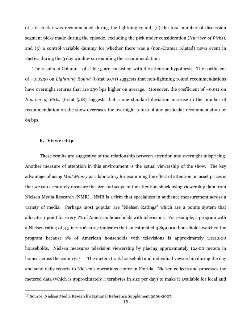
of 1 if stock i was recommended during the lightning round, (2) the total number of discussion
segment picks made during the episode, excluding the pick under consideration (Number of Picks),
and (3) a control variable dummy for whether there was a (non-Cramer related) news event in
Factiva during the 3 day window surrounding the recommendation.
The results in Column 1 of Table 5 are consistent with the attention hypothesis. The coefficient
of −0.0239 on Lightning Round (t-stat 10.71) suggests that non-lightning round recommendations
have overnight returns that are 239 bps higher on average. Moreover, the coefficient of −0.011 on
Number of Picks (t-stat 5.18) suggests that a one standard deviation increase in the number of
recommendation on the show decreases the overnight return of any particular recommendation by
65 bps.
b. Viewership
These results are suggestive of the relationship between attention and overnight mispricing.
Another measure of attention in this environment is the actual viewership of the show. The key
advantage of using Mad Money as a laboratory for examining the effect of attention on asset prices is
that we can accurately measure the size and scope of the attention shock using viewership data from
Nielsen Media Research (NMR). NMR is a firm that specializes in audience measurement across a
variety of media. Perhaps most popular are "Nielsen Ratings" which are a points system that
allocates 1 point for every 1% of American households with televisions. For example, a program with
a Nielsen rating of 3.5 in 2006-2007 indicates that an estimated 3,899,000 households watched the
program because 1% of American households with televisions is approximately 1,114,000
households. Nielsen measures television viewership by placing approximately 12,600 meters in
homes across the country.12 The meters track household and individual viewership during the day
and send daily reports to Nielsen's operations center in Florida. Nielsen collects and processes the
metered data (which is approximately 4 terabytes in size per day) to make it available for local and
12 Source: Nielsen Media Research's National Reference Supplement 2006-2007.

16
national broadcasting networks and cable channels who use the data to measure the success of their
programs and set advertising rates. During "sweeps" months, Nielsen supplements its metered data
collection with personal diaries that households fill out to describe their viewing habits each week.
Beyond the physical count of viewers, Nielsen also collects information about the households they
sample, including age, race, education and income class.
Our data consist of Nielsen's live daily viewership estimates for Mad Money which originally
airs at 6 p.m. EST each weekday (and reruns at 9 p.m. and midnight).13 Our data are broken down
by (1) the time of the show (6 p.m., 9 p.m. or midnight) and by (2) household income classes. Table 1
includes some summary statistics about our 6 p.m. viewership data. The average viewership in our
sample for the 6 p.m. show is 195,982 with a standard deviation of 51,607 households. Nielsen
breaks the viewership into income brackets: we have data on the number of households viewing each
episode with annual incomes less than $20K, between $20K and $30K, between $30K and $40K,
between $40K and $50K, between $50K and $60K, between $60K and $75K, and greater than
$75K. Defining high income viewers as those with household income above $60,000, we find the
average high income viewership in our sample for the 6 p.m. show is 134,503 households with a
standard deviation of 44,885 households.14
If individual traders who watch Mad Money are the noise traders of Barber and Odean
(2008), we should expect to find a positive relationship between the size of the attention shock
measured by Nielsen viewership and the size of the overnight mispricing. We find exactly that.
Column 2 of Table 5 augments Column 1 by adding total viewership in millions (Viewership).
Now the control variables include all of the independent variables in Column 1 (including
Lightning Round, Number of Picks, and News) and Viewership is the total number of households
who watched the show on day t according to NMR.
13 Nielsen also collects DVR or "Tivo" viewership estimates for households who record shows and watch them later. Only the live viewership estimates are used in our analysis. 14 We define high income households as those earning more than $60,000 because the median income for a four person family in the United States is $62,732. (Source: http://www.census.gov/hhes/www/income/4person.html ) All of our qualitative results are robust to using $75K or $50K as the high income cutoff.

17
The positive coefficient of 0.0584 (t-stat 1.80) on Viewership suggests that when more
people are exposed to the recommendation (as measured by viewership) the overnight return is
higher. A one standard deviation in total viewership leads to another 30 bps of overnight return.
This is some of our strongest evidence in support of the attention hypothesis of Barber and Odean
(2008): when we vary the size of the attention shock (which we can directly measure using
viewership) we also vary the size of the overnight mispricing.15
Interestingly, when we consider low income (annual income < $60,000) and high income
(annual income > $60,000) viewership in column 3 of Table 5, we find the dominant effect exists
among high income viewers. This is perhaps because high income individuals, who are likely to be
wealthy, have capital to execute a trade following an attention shock and are more likely to
participate in the market in the first place (see, e.g., Table 6 in Vissing-Jorgensen [2003]). A one
standard deviation increase in High Income Viewership increases abnormal overnight returns by 34
basis points. In contrast, we find no evidence of a relationship between the number of low income
individuals exposed to the recommendations and abnormal overnight returns. This evidence
suggests that attention shocks are not homogenous and that the composition of the cross-section of
traders who receive the shock matters for asset prices. In short, who observes an event may be just
as important as how many do.
c. Limits to Arbitrage
Arbitrageurs have a strong incentive to profit when prices deviate from fundamental
values. Therefore the size of the mispricing should be related to the frictions and forces that prevent
arbitrageurs from correcting any mispricing (Pontiff [1996] and Shleifer and Vishny [1997]). Here
15 It is also worth mentioning that our regression analysis likely underestimates the effect of attention on prices since we only observe variation in casual viewership. Since Webster and Washklag (1983) and Zubayr (1999) find evidence of both channel and program loyalty among television audience members, we can imagine that Cramer's viewers are either loyal viewers (who watch nearly every show) or casual viewers (who do not). By definition, time series variation in viewership only captures variation in casual viewership. Therefore, our regression estimates of the relationship between attention and prices will be driven by casual viewers. To the extent that loyal viewers are more likely to trade following a Cramer recommendation than casual viewers, we have underestimated the relationship between viewership and overnight return.

18
we consider several limits to arbitrage and ask whether the size of the mispricing is related to the size
of the ties that bind the arbitrageur.
We are not the first researchers to test whether arbitrage costs affect the mispricing of assets.
Previous researchers have looked at the relationship between potential limits to arbitrage and
various anomalies, including post-earnings announcement drift (Mendenhall [2004]), the book-to-
market effect (Ali, Hwang, and Trombley [2003]), and the accrual anomaly (Mashruwala, Rajgopal,
and Shevlin [2006]). Our setting differs in that we have a clear case of temporary mispricing
followed by convergence to fundamental value, whereas the other studies focus on anomalies that
may or may not be the result of market mispricing.
We begin by using three stock-specific variables that have been commonly used to proxy for
limits to arbitrage: illiquidity, size and idiosyncratic volatility. Small, illiquid stocks can have high
transaction costs relative to large, liquid stocks, and idiosyncratic volatility poses a holding cost that
an arbitrageur must bear. See Pontiff (2006) for a discussion on why idiosyncratic volatility should
affect arbitrageurs’ willingness to correct mispricing.
Our measure of idiosyncratic volatility is IdioVol, which is defined as the standard deviation
of the abnormal daily returns from days −34 through −5, where day 0 represents the day of the
recommendation. Our measure of Size is the NYSE-based size quintile that the stock is assigned to
when we match the stocks to size and book-to-market quintiles.
Finally, our measure of Illiquidity is developed by Amihud (2002). This measure is defined as:
Average | t|
t
where r is the stock return on day t and is the dollar volume on day t. The
average is calculated over all positive-volume days from days −34 to −5 (inclusive).

19
We are especially interested in the stocks with the most significant limits to arbitrage. Figure
3 considers these stocks in the event-time framework. Panel A considers the CAR around the
recommendation date for the smallest Size quintile of recommendations as well as recommendations
in the largest Illiquidity quintile. Panel B considers the highest IdioVol quintile as well as stocks that
are short-sale constrained (discussed below). If limits to arbitrage prevent arbitrageurs from
immediately correcting mispring, we should see the most dramatic spike/reversal patterns among
these sub-samples of recommendations. This is precisely what we find. For example, among the
smallest Size recommendations, stocks have a mean CAR above 6% shortly after Cramer’s
recommendation. However, within three months the mean CAR among small stocks falls below 0%.
Similar results are found among illiquid stocks and those with high idiosyncratic volatility.
In Table 5 we consider limits to arbitrage in the multivariate regression framework. We
divide the stocks into quintiles based on their Size, IdioVol and Illiquidity, and then regress the
abnormal overnight returns on our attention variables and dummies for the quintiles that the stock
belongs to for each of our three limits to arbitrage variables. For each of our regressions, the dummy
for the least significant limit to arbitrage quintile is omitted from the set of independent variables.
In column 4 of Table 5, we see report the results for the regression with Illiquidity fixed
effects. The coefficient for the largest Illiquidity is 4.9% (t-stat 11.8), which implies that liquidity
plays a large role in the overnight returns.
In Column 5, we add fixed effects for the NYSE-based Size quintile of the recommended
stock. The coefficient for the smallest quintile is 4.0% (t-stat 6.05), showing that the smallest stocks
experience much larger overnight returns following Cramer’s recommendations than do the largest
ones.
In Column 6, we add fixed effects for the IdioVol quintile. As predicted, the quintile of stocks
with the highest idiosyncratic volatilities has significantly larger overnight returns than the quintile
of stocks with the lowest idiosyncratic volatilities (1.5% difference, t-stat 3.49).

20
d. Short-Selling
Short-sale constraints are another potential limit to arbitrage. If an arbitrageur believes a
stock is trading above its fundamental value and he does not already own the stock, he must borrow
shares in order to sell the stock. Such borrowing can be costly, especially when there is a lot of
demand for borrowing. If short-sale constraints are an insignificant limit to arbitrage, these costs
should be unrelated to the level of mispricing. If, however, these costs limit arbitrageurs' ability to
correct mispricing, we should expect a correlation between the size of the mispricing and the cost of
short-selling.
To test these hypotheses we obtain equity lending data for a subset of our
recommendations from a data provider that is both a market maker in the equity loan market and a
data provider for major equity lenders. See Kolasinski, Reed, and Ringgenberg (2008) for a more
detailed description of the equity lending data. For every stock on every day, the lending database
reports the weighted average rebate rate calculated from the loan portfolios of 12 lenders. The cost
of shorting is measured by the difference between the federal funds rate and the rebate rate. (The
rebate rate is the interest rate paid on the collateral posted by the short seller when borrowing the
shares to sell.). For each recommendation, we define a variable called Specialness as the average
difference between these variables between days −34 and −5 (inclusive). As Reed (2007) argues, the
specialness of a stock “represents scarcity in the equity loan market on a daily basis."
The subsample of stocks for which we have short-selling data consists of 271
recommendations made between November 16, 2005 and August 4, 2006. Compared to the full
sample, these stocks have similar book-to-market ratios but are smaller.16 The mean (median) book-
to-market ratio is 0.44 (0.35), and the mean (median) market cap is $6.75 billion ($1.53 billion).
The average value of Specialness is 54.9 bps, with a standard deviation of 153.7 bps. The distribution
16 The stocks in this sample are smaller because Cramer tended to recommend smaller stocks during the time period in which we have short-selling data.
21
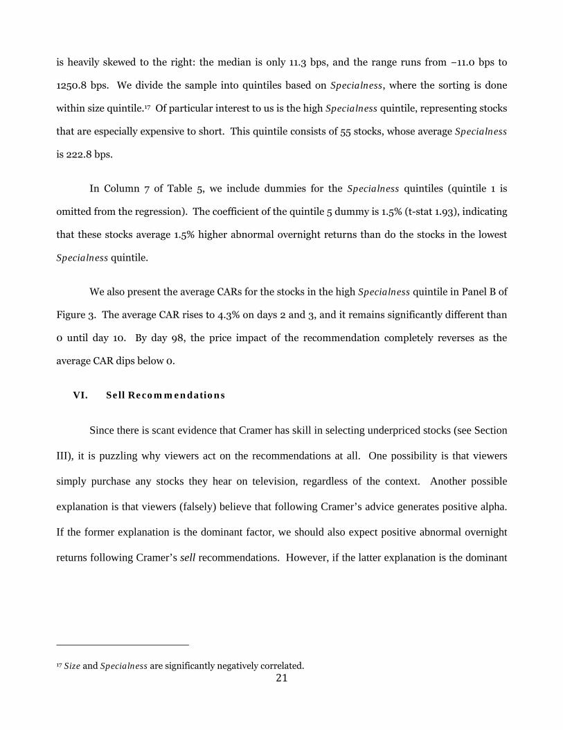
is heavily skewed to the right: the median is only 11.3 bps, and the range runs from −11.0 bps to
1250.8 bps. We divide the sample into quintiles based on Specialness, where the sorting is done
within size quintile.17 Of particular interest to us is the high Specialness quintile, representing stocks
that are especially expensive to short. This quintile consists of 55 stocks, whose average Specialness
is 222.8 bps.
In Column 7 of Table 5, we include dummies for the Specialness quintiles (quintile 1 is
omitted from the regression). The coefficient of the quintile 5 dummy is 1.5% (t-stat 1.93), indicating
that these stocks average 1.5% higher abnormal overnight returns than do the stocks in the lowest
Specialness quintile.
We also present the average CARs for the stocks in the high Specialness quintile in Panel B of
Figure 3. The average CAR rises to 4.3% on days 2 and 3, and it remains significantly different than
0 until day 10. By day 98, the price impact of the recommendation completely reverses as the
average CAR dips below 0.
VI. Sell Recommendations
Since there is scant evidence that Cramer has skill in selecting underpriced stocks (see Section
III), it is puzzling why viewers act on the recommendations at all. One possibility is that viewers
simply purchase any stocks they hear on television, regardless of the context. Another possible
explanation is that viewers (falsely) believe that following Cramer’s advice generates positive alpha.
If the former explanation is the dominant factor, we should also expect positive abnormal overnight
returns following Cramer’s sell recommendations. However, if the latter explanation is the dominant
17 Size and Specialness are significantly negatively correlated.

22
factor, we should see negative abnormal overnight returns following his sell recommendations, but
the returns should be less significant due to short sale constraints.18
To better understand why viewers are acting on the recommendations, we analyze the price
response to Cramer’s sell recommendations. Because YourMoneyWatch.com does not supply sell
recommendations, we gather them from an alternate source (http://www.madmoneyrecap.com/)
which also catalogues Cramer recommendations. From MadMoneyRecap, we gather 1,445 first-
time sell recommendations between July 1, 2005 and December 24, 2008.19 Like the buy
recommendations, these stocks tend to be recent winners with low book-to-market ratios. 277 of the
sell recommendations (19%) are in the top momentum decile, and 546 of the 1445 recommendations
(38%) are in the smallest book-to-market quintile. The sell recommendations differ from the buy
recommendations in that they are most likely to fall in the smallest size quintile: 386 of the
recommendations (27%) lie in the smallest quintile, more than any other quintile.
We find a clear asymmetry between buy and sell recommendations, suggesting that
viewers do not respond the same way to sell recommendations as they do to buy
recommendations. When we compare all first‐time buy recommendations with all first‐time
sell recommendations, we see a considerable asymmetry (Figure 4). First-time buy
recommendations have a large overnight return (2.4%) while the magnitude of the overnight return
is small following first-time sell recommendations (−0.29%). There is also no detectable post-
recommendation trend in sell-recommendation returns. The evidence supports the view that an
18 For sell recommendations, viewers can easily act on the recommendation only if they already own shares of the stock. The idea that short selling is more difficult than purchasing shares and therefore attention can produce asymmetries between the buying and selling of stocks by individual traders also appears in Barber and Odean (2008). 19 The larger number of sell recommendations from does not indicate that Cramer makes more sell recommendations. Casual observation suggests that our source for sell recommendations (http://www.madmoneyrecap.com/) has a weaker standard for what constitutes a sell recommendation than our source for buy recommendations.

23
attention shock in the form of a sell recommendation has little effect on returns, perhaps because it
is difficult for retail traders to short Cramer’s sell recommendations.
VII. Conclusion
We find considerable evidence that Jim Cramer causes individual stock prices to
temporarily rise when he recommends them on his CNBC show Mad Money. The causal
interpretation is supported by the fact that prices rise in the precise hour his show airs and for
stocks that have no other news. Interestingly, this effect exists even though there is no
evidence of information in the recommendations. Calendar‐time portfolios which go long the
recommendations before the show airs find no long‐term alpha. This suggests the initial price
spikes constitute mispricing.
We also find that the size of the mispricing varies considerably in the cross‐section.
When attention towards the recommendations is high or limits to arbitrage are great, we find
much greater mispricing. Moreover, the size of the cross‐sectional variation is large. In a few
cases, prices spike by more than 20% overnight (maximum = 32.8%, Table 3) following a Mad
Money recommendation but limits to arbitrage still prevent “smart money” from correcting
such distortions.
Taken together, the evidence here suggests that media endorsements of individual
stocks may lead to substantial mispricing (Huberman and Regev [2001]) and that limits to
arbitrage is a powerful friction which allows mispricing to persist.

24
References
Ali, A., L. Hwang and M. Trombley (2003): “Arbitrage Risk and the Book-to-Market Anomaly,”
Journal of Financial Economics, 69, 355-373.
Amihud, Y. (2002): “Illiquidity and Stock Returns: Cross-section and Time Series Effects,” Journal
of Financial Markets, 5, 31-56.
Barber, B., and D. Loeffler (1993): “The “Dartboard” Column: Second-Hand Information and Price
Pressure,” The Journal of Financial and Quantitative Analysis, 28, 273-284.
Barber, B., and T. Odean (2008): “All that Glitters: The Effect of Attention and News on the Buying
Behavior of Individual and Institutional Investors,” The Review of Financial Studies, 21, 785-
818.
Chan, W. (2003): “Stock Price Reaction to News and No News: Drift and Reversal after Headlines,”
Journal of Financial Economics, 70, 223-260.
Chen, J., H. Hong, and J. Stein (2001): “Forecasting Crashes: Trading Volume, Past Returns, and
Conditional Skewness in Stock Prices,” Journal of Financial Economics, 61, 345-381.
DellaVigna, S., and J. Pollet (2009): “Investor Inattention and Friday Earnings Announce-ments,"
Journal of Finance, 64, 709-749.
Engelberg, J. (2008): “Costly Information Processing: Evidence from Earnings Announcements,"
Working Paper.
Engelberg, J., and C. Parsons (2009): “The Causal Impact of Media in Financial Markets," Journal of
Finance, forthcoming.
Fang, L., and J. Peress (2008): “Media Coverage and the Cross-Section of Expected Returns,"
Journal of Finance, 64, 2023-2052.
Gervais, S., R. Kaniel, and D. Mingelgrin (2001): “The High-Volume Return Premium," The Journal
of Finance, 56, 877-919.
Grullon, G., G. Kanatas, and J. Weston (2004): “Advertising, Breadth of Ownership, and Liquidity,"
The Review of Financial Studies, 17, 439-461.

25
Hirshleifer, D., S. Lim, and S. Teoh (2009): “Driven to Distraction: Extraneous Events and
Underreaction to Earnings News,” Journal of Finance, 64, 2289–2325.
Hou, K., L. Peng, and W. Xiong (2008): “A Tale of Two Anomalies: The Implications of Investor
Attention for Price and Earnings Momentum," Working Paper.
Huberman, G., and T. Regev (2001): “Contagious Speculation and a Cure for Cancer: A Nonevent
that Made Stock Prices Soar," The Journal of Finance, 56, 387-396.
Keasler, T., and C. McNeil (2008): “Mad Money Stock Recommendations: Market Reaction and
Performance," Journal of Economics and Finance, 34, 1-22.
Kolasinski, A., A. Reed, and M. Ringgenberg (2008): “A Multiple Lender Approach to Understanding
Supply and Demand in the Equity Lending Market," Working Paper.
Liu, P., S. D. Smith, and A. Syed (1990): “Stock Price Reactions to The Wall Street Journal's
Securities Recommendations," The Journal of Financial and Quantitative Analysis, 25, 399-
410.
Mashruwala, C., S. Rajgopal, and T. Shevlin (2006): “Why is the Accrual Anomaly not Arbitraged
Away? The Role of Idiosyncratic Risk and Transaction Costs,” Journal of Accounting and
Economics, 42, 3-33.
Mendenhall, R. (2004): “Arbitrage Risk and Post-Earnings Announcement Drift,” Journal of
Business, 77, 875-894.
Neumann, J., and P. Kenny (2007): “Does Mad Money make the market go mad?" The Quarterly
Review of Economics and Finance, 47, 602-615.
Pontiff, J. (1996): “Costly arbitrage: Evidence from Closed-end Funds," The Quarterly Journal of
Economics, 111, 1135-1152.
Pontiff, J. (2006): “Costly Arbitrage and the Myth of Idiosyncratic Risk,” Journal of Accounting and
Economics, 42, 35-52.
Reed, A. (2007): “Costly Short Selling and Stock Price Adjustment to Earnings Announcements,"
Working Paper.

26
Reuter, J., & Zitzewitz, E. (2006). Do ads influence editors? Advertising and bias in the financial
media. Quarterly Journal of Economics, 121(1), 197-227.
Shleifer, A., and R. Vishny (1997): “The Limits of Arbitrage," The Journal of Finance, 52, 35-55.
Tetlock, P. (2008): “All the News Thats Fit to Reprint: Do Investors React to Stale Information?,"
Working Paper.
Vega, C. (2006): “Stock Price Reaction to Public and Private Information," Journal of Financial
Economics, 82, 103-133.
Vissing-Jorgensen, A. (2003): “Perspectives on Behavioral Finance: Does “Irrationality" Disappear
with Wealth? Evidence from Expectations and Actions," NBER Macroeconomics Annual.
Webster, J., and J. Washklag (1983). "A Theory of Television Program Choice". Communication
Research, 10, 430-446.
Zubayr, C. (1999). "The Loyal Viewer? Patterns of Repeat Viewing in Germany". Journal of
Broadcasting & Electronic Media, 43, 346-363

27
Figure 1: Intraday Returns and Volume Surrounding Recommendations In Panel A we plot intraday returns on the day of Cramer’s recommendation. Prices are based on recorded trades in the NASDAQ’a historical ITCH data feed, which includes after hours trades on INET. Our sample consists of the 382 stocks with at least one trade on the ITCH data prior to 6 PM on the day of the recommendation. In Panel B we plot intraday returns based on whether the stock had a news announcement in Factiva during the 3-day window surrounding Cramer’s recommendation. The News sample consists of 187 stocks, and the No News sample consists of 195 stocks. In Panels C and D we plot intraday turnover (scaled by 1,000) per thirty minute interval based on trading data from NASDAQ’s historical ITCH data feed, which includes after hours trading on INET. In Panels A and C, the 95% bootstrap confidence interval is plotted in dashed lines.
PANEL A: Intraday CARs
PANEL B: CARs With and Without News
-0.005
0
0.005
0.01
0.015
0.02
0.025
0.03
0.035
0.04
0.045
3:30 4:00 4:30 5:00 5:30 6:00 6:30 7:00 7:30 8:00
Ret
urn
Time
Cumulative Return95% CI
-0.005
0
0.005
0.01
0.015
0.02
0.025
0.03
0.035
0.04
0.045
3:30 4:00 4:30 5:00 5:30 6:00 6:30 7:00 7:30 8:00
Ret
urn
Time (p.m.)
No News
News

28
PANEL C: Intraday Volume
PANEL D: Intraday Volume With and Without News
0
0.1
0.2
0.3
0.4
0.5
0.6
0.7
3:30 4:00 4:30 5:00 5:30 6:00 6:30 7:00 7:30 8:00
Tu
rno
ver
Time (p.m.)
30-minute Turnover
95% CI
0
0.1
0.2
0.3
0.4
0.5
0.6
0.7
3:30 4:00 4:30 5:00 5:30 6:00 6:30 7:00 7:30 8:00
Tu
rno
ver
Time (p.m.)
No News
News

29
Figure 2: CARs Sorted by News and Overnight Return We plot average cumulative abnormal returns (CARs) around Cramer’s recommendations in event time, where Day 1 is the first trading day following the recommendation. Abnormal return on a given day is computed as the stock’s return minus its matched portfolio’s equal weighted return. The solid line in Panel A is based on the entire sample consisting of the 826 buy recommendations of non-ADRs that can be matched to size and book to market portfolios. The dashed line in Panel A is based on the 165 observations with the highest overnight return (top quintile). The solid line in Panel B is based on the sample consisting of 464 buy recommendations with no news event in the 3 day window surrounding the recommendation. The dashed line in Panel B is based on the sample consisting of 362 buy recommendations with a news event in the 3 day window surrounding the recommendation.
PANEL A
PANEL B
‐3.00%
‐2.00%
‐1.00%
0.00%
1.00%
2.00%
3.00%
4.00%
5.00%
6.00%
7.00%
8.00%
‐5 5 15 25 35 45 55 65 75 85 95
CAR
Days
All
Highest Overnight Return
‐2.00%
‐1.00%
0.00%
1.00%
2.00%
3.00%
‐5 5 15 25 35 45 55 65 75 85 95
CAR
Days
No News
News

30
Figure 3: CARs and Limits to Arbitrage We plot average cumulative abnormal returns (CARs) around Cramer’s recommendations in event time, where Day 1 is the first trading day following the recommendation. Abnormal return on a given day is computed as the stock’s return minus its matched portfolio’s equal weighted return. Panel A is based on the buy recommendations in the smallest Size quintile (solid line) and the highest Illiquidity quintile (dashed line). Panel B is based on the quintile of buy recommendations with the highest idiosyncratic volatility or IdioVol (solid line) and the highest short-selling constraints or Specialness (dashed line).
PANEL A
PANEL B
‐3.00%
‐2.00%
‐1.00%
0.00%
1.00%
2.00%
3.00%
4.00%
5.00%
6.00%
7.00%
‐5 5 15 25 35 45 55 65 75 85 95
CAR
Days
Small
Illiquid
‐3.00%
‐2.00%
‐1.00%
0.00%
1.00%
2.00%
3.00%
4.00%
5.00%
6.00%
7.00%
‐5 5 15 25 35 45 55 65 75 85 95
CAR
Days
High Idiosyncratic Volatility
Short‐Sale Constrained

31
Figure 4: Sell vs. Buy Recommendations We plot cumulative abnormal returns (CARs) for the first-time sell recommendations and the first-time buy recommendations Jim Cramer issued between July 1, 2005 and December 24, 2008. Day 1 is the first trading day following the recommendation. Abnormal return on a given day is computed as the stock’s return minus its matched portfolio’s equal weighted return.
‐2.00%
‐1.00%
0.00%
1.00%
2.00%
3.00%
‐5 5 15 25 35 45 55 65 75 85 95
CAR
Days
Buy Recommendations
Sell Recommendations

32
Table 1: Summary Statistics
Total viewership is the total number of households (in thousands) viewing the 6 PM ET showing of Mad Money. High (Low) Income Viewership is the number of households earning more than (less than) $60,000 per year viewing the 6 PM ET showing of Mad Money. Size is the market cap, in billions USD, on the last trading day prior to the recommendation. Book-to-market Ratio is defined in Section 2. 50-Day CAR is the cumulative abnormal return in the 50 trading days before the recommendation is made (including the day of the show). Specialness is the average difference between the federal funds rate and the rebate rate between event time days -5 and -34.
Number of
Observations Mean Standard Deviation Minimum
20th Percentile Median
80th Percentile Maximum
Total Viewership 386 195.982 51.607 66 154 192 234 650
Low income Viewership
386 61.479 22.977 9 43 60 78 171
High Income Viewership
386 134.503 44.885 20 97 136 166 479
Size 826 11.866 29.885 0.013 0.587 2.478 12.660 365.839
Book-to-Market Ratio 826 0.414 0.590 -9.689 0.185 0.349 0.599 9.103
50-Day CAR 826 0.084 0.167 -0.437 -0.034 0.062 0.185 1.541
Specialness 271 0.549% 1.537% -0.110% -0.031% 0.113% 0.423% 12.508%

33
Table 2: Before Recommendation Portfolio Returns
The panels present regression results when daily, calendar-time portfolio excess returns are regressed on standard factors. Portfolio returns are calculated from equal-weighted portfolios with returns reported in basis points. Portfolios go long Mad Money recommendations at the market close before the recommendations are made. Stocks stay in the portfolio for 50, 100, 150, 200 and 250 days in columns 1,2,3,4 and 5 respectively. The top panel presents regression results when the calendar-time portfolios are regressed against 1 factor: the excess market return. The bottom panel presents regression results when the calendar-time portfolios are regressed against the standard four factors. All daily factor returns are taken from Ken French’s website. Standard errors are in brackets. *, **, and *** represent significance at the 10%, 5% and 1% levels, respectively.
PANEL A: MARKET MODEL
Hold 50 Days Hold 100 Days Hold 150 Days Hold 200 Days Hold 250 Days
Intercept 0.104 ‐0.427 ‐0.336 ‐0.163 0.990[3.882] [3.208] [2.249] [1.902] [1.729]
MKT ‐ RF 0.893*** 0.882*** 0.954*** 1.004*** 1.022***[0.046] [0.035] [0.028] [0.023] [0.020]
Observations 939 987 987 987 987R‐Squared 0.6062 0.6773 0.8334 0.8859 0.9067
PANEL B: FOUR FACTOR MODEL
Hold 50 Days Hold 100 Days Hold 150 Days Hold 200 Days Hold 250 Days
Intercept 0.287 0.049 ‐0.144 ‐0.095 1.008[3.463] [2.754] [1.858] [1.492] [1.271]
MKT ‐ RF 1.062*** 1.055*** 1.047*** 1.065*** 1.068***[0.045] [0.026] [0.023] [0.020] [0.015]
SMB 0.589*** 0.496*** 0.517*** 0.529*** 0.542***[0.105] [0.059] [0.046] [0.038] [0.031]
HML ‐0.016 ‐0.107 ‐0.075 ‐0.074* ‐0.064*[0.118] [0.071] [0.050] [0.042] [0.035]
MOM 0.332*** 0.293*** 0.143*** 0.077*** 0.051***[0.062] [0.043] [0.030] [0.021] [0.017]
Observations 939 987 987 987 987R‐Squared 0.6857 0.7581 0.8849 0.9294 0.9493

34
Table 3: Abnormal Overnight Returns with and without News
We report statistics on the abnormal overnight returns following Cramer’s buy recommendations. Our sample consists of the 826 first-time recommendations Cramer issued between July 28, 2005 and February 6, 2009. Abnormal overnight returns are defined as the difference between the overnight return of the recommended stock and the average overnight return in the stock’s size and book-to-market matched portfolio. The Recommendations with News sample consists of the stock recommendations for which there was a (non-Cramer related) news article appearing in Factiva during the three day window surrounding the recommendation date. The Recommendations without News sample consists of the other recommendations.
Number of Observations Mean
Standard Deviation Minimum
20th Percentile Median
80th Percentile Maximum
All Recommendations 826 2.405% 3.696% -10.465% 0.151% 1.179% 3.963% 32.809%
Recommendations with News 362 1.880% 3.215% -4.973% 0.060% 0.729% 3.047% 20.182%
Recommendations without News
464 2.815% 3.987% -10.465% 0.233% 1.675% 4.563% 32.809%

35
Table 4: After Recommendation Portfolio Returns
The panels present regression results when daily, calendar-time portfolio excess returns are regressed on the standard four factors. Portfolio returns are calculated from equal-weighted portfolios with returns reported in basis points. Portfolios go long Mad Money recommendations at the market close after the recommendations are made. Stocks stay in the portfolio for 50, 100, 150, 200 and 250 days in columns 1,2,3,4 and 5 respectively. The top panel presents regression results for the entire sample of recommendations and the bottom panel presents results for the set of recommendations which are in the highest quintile of overnight return. All daily factor returns are taken from Ken French’s website. Standard errors are in brackets. *, **, and *** represent significance at the 10%, 5% and 1% levels, respectively.
PANEL A: All Recommendations
Hold 50 Days Hold 100 Days Hold 150 Days Hold 200 Days Hold 250 Days
Intercept ‐4.173 ‐2.674 ‐2.520 ‐2.400* ‐1.282 [3.494] [2.737] [1.814] [1.443] [1.221]
MKT ‐ RF 1.056*** 1.059*** 1.049*** 1.066*** 1.068*** [0.047] [0.026] [0.023] [0.020] [0.015]
SMB 0.552*** 0.479*** 0.500*** 0.514*** 0.528*** [0.108] [0.059] [0.045] [0.038] [0.031]
HML 0.015 ‐0.100 ‐0.071 ‐0.072* ‐0.064* [0.119] [0.071] [0.050] [0.041] [0.034]
MOM 0.334*** 0.292*** 0.138*** 0.073*** 0.048*** [0.063] [0.043] [0.029] [0.021] [0.017]
Observations 938 986 986 986 986 R‐Squared 0.681 0.7619 0.8905 0.9342 0.9532
PANEL B: High Overnight Returns
Hold 50 Days Hold 100 Days Hold 150 Days Hold 200 Days Hold 250 Days
Intercept ‐13.884** 0.082 ‐7.228 ‐6.510* ‐3.704 [6.500] [5.544] [4.433] [3.707] [2.963]
MKT ‐ RF 1.210*** 1.319*** 1.244*** 1.262*** 1.261*** [0.102] [0.085] [0.058] [0.053] [0.042]
SMB 0.397* 0.441*** 0.569*** 0.641*** 0.660*** [0.206] [0.152] [0.117] [0.103] [0.079]
HML 0.016 ‐0.395* ‐0.333** ‐0.221* ‐0.182* [0.280] [0.213] [0.141] [0.119] [0.096]
MOM 0.509*** 0.321*** 0.286*** 0.152*** 0.013 [0.096] [0.078] [0.062] [0.049] [0.037]
Observations 837 910 960 986 986 R‐Squared 0.4327 0.5601 0.6328 0.7354 0.8294

36
Table 5: Determinants of Overnight Mispricing
We report the results of regressions in which the dependent variable is the abnormal overnight return. Abnormal overnight return is defined as the return of the stock minus the average return of all stocks in the size and book-to-market matched portfolio. Lightning Round is a dummy for whether the recommendation was made during the lightning round portion of the show. Number of Picks is the number of discussion segment (i.e., non-lightning round) picks (in units of 10) Cramer makes on the day of the recommendation, excluding the recommendation under consideration. News is a dummy for whether a (non-Cramer related) news article appears in Factiva during the three day window surrounding the recommendation date. Total Viewership is the number of households, in millions, who viewed the 6 PM ET episode of the show. High (Low) Income Viewership is the number of households, in millions, with annual incomes greater than $60,000 (less than $60,000) viewing the 6 PM ET episode of the show. High Illiquidity (High Idiosyncratic Volatility) Dummy is a dummy for the stock being in the highest illiquidity (idiosyncratic volatility) quintile. Small Size Dummy is a dummy for the stock being in the smallest quintile based on NYSE cutoffs. Short Sale Constraint Dummy is a dummy for the stock being in the quintile with the highest Specialness. The regressions in Columns 4-7 also include dummies for Illiquidity quintiles 2, 3, and 4. Similarly, the regressions in Columns 5-7 also include dummies for Size quintiles 2, 3, and 4, the regressions in Columns 6 and 7 include dummies for IdioVol quintiles 2, 3, and 4, and the regression in Column 7 includes dummies for Specialness quintiles 2, 3, and 4. The coefficients of these dummies are omitted to make the table more reader-friendly. Robust standard errors are clustered by recommendation date and are shown in brackets. *, **, and *** denote statistical significance at the 10%, 5%, and 1% level, respectively.

37
Dependent Variable: Abnormal Overnight Return
Lightning Round -0.024*** -0.024*** -0.024*** -0.017*** -0.016*** -0.016*** -0.024***
[0.002] [0.002] [0.002] [0.002] [0.002] [0.002] [0.003]
Number of Picks -0.011*** -0.011*** -0.010*** -0.007*** -0.006*** -0.006*** -0.009*
[0.002] [0.002] [0.002] [0.002] [0.002] [0.002] [0.005]
News -0.008*** -0.008*** -0.008*** -0.001 -0.001 -0.001 -0.002
[0.003] [0.003] [0.003] [0.002] [0.002] [0.002] [0.004]
Total Viewership 0.058*
[0.032]
High Income Viewership 0.076** 0.074** 0.075** 0.067** 0.181**
[0.037] [0.035] [0.033] [0.034] [0.073]
Low Income Viewership -0.003 -0.030 -0.025 -0.009 0.077
[0.060] [0.053] [0.053] [0.052] [0.124]
High Illiquidity Dummy 0.049*** 0.013* 0.014** 0.020
[0.004] [0.007] [0.007] [0.013]
Small Size Dummy 0.040*** 0.033*** 0.036***
[0.007] [0.007] [0.013]
High Idiosyncratic Volatility Dummy 0.015*** 0.002
[0.0078] [0.0078]
Short Sale Constraint Dummy 0.015*
[0.008]
Observations 826 826 826 826 826 826 271
R-squared 0.12 0.12 0.12 0.34 0.37 0.39 0.44