market institutions,prices and distributionof surplus: a...
TRANSCRIPT

Market institutions, prices and distribution of surplus:
a theoretical and experimental investigation
Nejat Anbarci
Department of Economics
Deakin Business School
Geelong VIC 3220, Australia
Nick Feltovich∗
Department of Economics
Monash University
Clayton VIC 3800, Australia
February 22, 2016
Abstract
We examine three common market institutions for exchanging goods, using theory and an experiment. Under
non–negotiable price posting (“posting”), sellers post fixed prices that are seen by buyers who then choose which
seller to visit. Under “haggling”, prices are not posted, but emerge via negotiation or bidding depending on how
many potential trading partners a seller has. Under “flexible pricing”, prices are posted but can be negotiated
upwards or downwards like under haggling. We consider 2–buyer–2–seller (2x2) and 3–buyer–3–seller (3x3)
markets, but capacity constraints mean that local market tightness can vary; in particular, a seller at a given time
may face excess demand, excess supply or neither.
Behaviour in the experiment is largely, but not completely, in line with our theoretical predictions. Efficiency
is highest under posting, though differences become smaller with time and experience. Transaction prices are
highest under haggling and lowest under posting, while buyers’ surplus has the reverse ordering. Sellers fare best
under haggling in the 3x3 market, but prefer posting in the 2x2 market (as higher efficiency under posting offsets
the lower transaction prices). When there is local excess demand, sellers appropriate a majority of the surplus, but
substantially less than the predicted amount. When there is no local excess demand, bargaining tends to favour
the seller relative to the predictions of standard bargaining theory.
Journal of Economic Literature classifications: D83, D43, E03, C78, C90.
Keywords: directed search; posted prices; frictions; institutions; bargaining; auction.
∗Corresponding author. Financial support from the Australian Research Council (DP140100274) and Deakin University is gratefully
acknowledged. We thank participants at the 2016 Australian Economic Theory Workshop, Simon Grant, Benoit Julien, Matthew Leister and
Sephorah Mangin for helpful suggestions and comments.

Determination of the prices of goods and services has been one of the most fundamental, widespread, and long–
lasting questions in economics.1 Historically, much of the study of how prices are formed in markets has placed little
emphasis on the markets themselves. The classical analysis of perfectly competitive markets either ignores market
features as irrelevant or posits mechanisms (Cournot tatonnement, Walrasian auctioneer) that no–one believes to
exist. The theory of industrial organisation has had marked success in understanding the connection between prices
and some aspects of the market, such as the numbers of buyers and sellers, the presence of search costs, or the
degree of substitutability between firms’ products. However, other aspects have received much less attention, such
as whether prices are fixed or negotiable, whether and by whom they are posted (buyers, sellers, or neither), and
whether buyers visit sellers, the reverse, or neither. Many combinations of these factors exist in real markets.
Indeed, heterogeneity in these market institutions exists not only economy–wide, but also for particular goods. A
prime example is housing: in the same region, houses can be sold by auction, by bilateral negotiation between the
seller and individual buyers, and by a fixed posted price. Items on internet shopping websites can often be found
both for auction and at a fixed posted price, and in most big cities, the same souvenir t–shirt can be bought at a
posted price in souvenir shops and by negotiation at market stalls.
Understanding how market institutions have evolved, what their effects are, and how they can co–exist for in-
dividual goods, is clearly a monumental task. In this paper, we take a small step toward this understanding. We
consider a particular (hypothetical) good, we vary the market institution under which it is traded, and we compare
the outcomes. We complement our theoretical analysis with an empirical analysis based on a lab experiment. Using
the lab allows us to minimise issues of selection and endogeneity; to have more precise control over product char-
acteristics, seller costs, buyer values, and agents’ information; and to record aspects of outcomes that may not be
observable in the field, such as those involving units that are not traded.
We keep the underlying setting simple; this obviously entails a cost in realism, but gains us theoretical tractability,
and one has to start somewhere. Our markets are adapted from the competitive–search or directed–search settings
of Shimer (1996), Moen (1997), and Burdett, Shi and Wright (2001), especially the last of these. In these settings,
sellers compete for buyers by posting and committing to selling mechanisms, and buyers direct their search based on
these posted mechanisms. In particular, Burdett, Shi and Wright’s capacity–constrained sellers post uniform prices
that are observed by buyers who then simultaneously choose which seller to visit.
For understanding the effects of market institutions, directed search provides at least two advantages over a
reduced–form competitive–market assumption. First, frictions are possible and indeed likely, due to the combina-
tion of capacity constraints and the coordination problem amongst buyers: even though all potential exchanges are
mutually profitable, some buyers will be unable to buy and some sellers will be unable to sell. Thus, rather than
some level of efficiency being assumed, it will emerge from the solution to the model, and will be measured in
the experiment. Second, even though all of our markets will have equal numbers of buyers and sellers – and thus
market–wide, there will be neither excess demand nor excess supply – the realisations of buyers’ visit choices will
mean that some sellers will face local excess demand and others will not.
We consider three market institutions; this is obviously an incomplete sampling of the institutions in existence,
but arguably covers the most prevalent ones during the last century or so.2 Under non–negotiable price posting
1For example, the “diamonds–water paradox” mentioned in many introductory economics textbooks dates back at least to Adam Smith
(1776).2Bargaining can be traced back to 6000 B.C. (see http://www.barternewyork.net/history-of-bartering.html). Auc-
tions are very old as well: Milgrom and Weber (1982), relying on the Greek historian Herodotus, report that they date back to around the fifth
1

(which we will often simply call “posting”), sellers post prices which are observed by buyers prior to the visit
choice, and any trade is at the posted price. Under negotiated prices (“haggling”), no prices are posted, so the price
is set by bilateral bargaining (if a seller is visited by one buyer) or auction (if a seller is visited by multiple buyers).
Under price posting with negotiation (“flexible prices”), sellers post prices that are observed by buyers, but these
prices are non–binding: they can be revised downward (by bilateral bargaining) or upward (by auction), depending
on how many buyers visit the seller.3 While our posting treatment is a straightforward application of Burdett, Shi and
Wright’s (2001) model (and has been studied experimentally before: see Cason and Noussair, 2007, and Anbarci and
Feltovich, 2013), our flexible–pricing treatment represents the first attempt to study flexible prices in an experimental
directed–search environment.
Our setting departs from the theoretical framework established by Shimer (1996), Moen (1997), and Burdett, Shi
and Wright (2001) in two minor but noteworthy ways. First, in these earlier models, meetings between buyers and
sellers are one–on–one: each seller interacts with at most one buyer. In our haggling and flexible–pricing institutions,
by contrast, we allow for many–on–one meetings – in the form of auctions – when multiple buyers visit the same
seller. Second, our haggling institution allows random rather than directed search, since buyers make their visit
choices without observing posted prices (or any other information).
In Section 2, we theoretically analyse these three market institutions for two market sizes: 2 (sellers) x 2 (buyers)
and 3x3; we also use these sizes in our experiment. Theoretical analysis is complicated by the existence of multiple
equilibria, but under the typical simplifying assumptions used in this literature, we obtain predictions for efficiency
and transaction prices, and consequently the welfare of buyers or sellers, in all three market institutions.
Our experimental results, described in Section 4, are largely but not completely in line with our theoretical
predictions. In both 2x2 and 3x3 markets, observed efficiency is highest under posting, though the difference is small
and diminishes over time, consistent with the theoretical prediction of no difference across institutions. Observed
transaction prices in both markets are highest under haggling and lowest under posting. In the 3x3 market, this is
exactly the predicted ordering. In the 2x2 market, however, it is only partly consistent with the theory, since prices
under haggling and flexible pricing were predicted to be equal to each other, and both higher than under posting.
Finally, haggling yields the highest seller surplus in both markets, while posting yields the highest buyer surplus; both
of these results are consistent with the theory. This broad support for the theory in our market results is despite the
presence of systematic and substantial deviations from standard theoretical predictions in the bargaining and auction
stages under haggling and flexible pricing (see Section 4.1), and suggestive evidence of additional deviations in the
stage where buyers choose which seller to visit under posting and flexible pricing (see Section 4.2).
1 Literature review
We limit our discussion here to the most important and most closely related work to ours – besides that already
mentioned above – to save space and to avoid repeating the literature reviews of others.
century B.C.. In contrast, the use of posted prices by sellers is a relatively recent phenomenon, to our knowledge having begun in 1823 when
Alexander Stewart introduced posted prices in his “Marble Dry Goods Palace” in New York (see Scull and Fuller, 1967).3Both upward and downward flexibility are possible. For example, Han and Strange (2014) showed that during the US housing boom
between 2003 and 2006, 13.5 percent of houses sold above the asking price and 57.1 percent sold below the asking price. Even during the
2007–2010 housing bust, there were non–trivial fractions of both increases and decreases: 8.2 percent sold above the asking price and 74.3
percent sold below the asking price. See also Case and Shiller’s (2003) Table 13.
2

There is a theoretical literature dedicated to comparisons of the three fundamental exchange mechanisms – price
posting, bargaining, and auctions – that make up the market institutions we investigate. This literature is split into
two strands. Within the first one, which considers large numbers (continua) of buyers and sellers, Lu and McAfee
(1996) and Kultti (1999) conduct comparative analyses of bargaining versus auctions and auctions versus price
posting, respectively. Lu and McAfee (1996) use an evolutionary framework and find that bargaining is unstable
under a wide class of evolutionary dynamics, leading auctions to be selected as the only stable equilibrium outcome.
Along similar lines, Kultti (1999) finds that auctions and posted prices are equivalent in that agents’ expected utilities
are the same in both markets. Within the second strand, which considers finite and often small numbers of buyers
and sellers, Julien, Kennes and King (2001) show that sellers’ expected payoffs are higher under auctions than under
price posting in any finite–sized market, though the difference declines monotonically with market size. Julien,
Kennes and King (2002), in a model with two buyers and two sellers, consider three exchange mechanisms: posted
prices, and auctions with and without reserve prices. They show that for sellers, choosing to auction with a reserve
price dominates the other two options: it maximises profit irrespective of which mechanism the other seller chooses.
There is also a theoretical literature focussing specifically on flexible posted prices. Albrecht, Gautier, and
Vroman (2006) and Julien, Kennes, and King (2000) consider labour markets, so that sellers are job seekers, buyers
are (firms with) vacancies, and prices are wages. The main finding in both studies is that sellers sell at a high price
if they are visited by two or more buyers; otherwise, they sell at a low price. This is because buyers who visit the
same seller compete by bidding the posted price up to their reservation value, as they would in an auction (as in
our haggling and flexible–pricing market institutions when a seller is visited by more than one buyer). Thus, the
high price is insensitive to realised demand beyond two buyers visiting a seller. Camera and Selcuk (2009) consider
an alternative model where renegotiated prices are an increasing function of demand. There, a seller or buyer
can request renegotiation of the posted price, which then initiates a potentially infinite alternating–offer bargaining
subgame. Camera and Selcuk identify conditions under which fixed–price trading emerges in equilibrium, even if
posted prices are non–binding.4
We know of no previous experimental work comparing the market institutions we examine here, but there are
now several experimental studies involving directed search. Cason and Noussair (2007) and Anbarci and Feltovich
(2013) test Burdett, Shi and Wright’s (2001) model against alternative models for their ability to characterise subject
behaviour in directed–search environments. Anbarci, Dutu and Feltovich (2015) construct a model of the infla-
tion tax by fitting Burdett, Shi and Wright’s model into the money–search environment in the vein of Lagos and
Wright (2005), which they then test experimentally. Helland, Moen and Preugschat (2015) and Anbarci and Fel-
tovich (2015a) test Lester’s (2011) conjecture that in some finite markets, improving buyers’ price information can
counter–intuitively lead to higher prices. Finally, Kloosterman (2015) tests various theoretical predictions involving
a directed–search labour market with heterogeneous buyers (firms).
2 Theoretical background
We consider mxn markets, with m ≥ 2 sellers and n ≥ 2 buyers. Sellers produce a homogeneous, indivisible,
perishable good and are capacity–constrained; production is costless for the first unit and impossible beyond that.
Buyers are identical, each with valuation U > 0 for the first unit and zero for any additional unit. We consider
4See also Stacey (2015), who analyses a similar setting and tests it using field data.
3

three market institutions. Under posting, sellers simultaneously post prices in [0, U]. Buyers observe these prices
and simultaneously choose a seller to visit. A seller visited by no buyers is unable to sell, while a seller visited by
at least one buyer sells at the posted price; in the case of multiple buyers, one is chosen randomly to buy, while the
other buyers are unable to buy.
Under our second pricing institution, haggling, sellers do not post prices, so buyers simultaneously choose a
seller to visit based on no information at all. A seller visited by no buyers is unable to sell. If exactly one buyer
visits a seller, they bargain over the price. Bargaining is modelled by a variant of the Nash (1953) demand game,
in which the buyer and seller simultaneously make a single price choice in [0, U ]. If the buyer’s “bid price” is at
least as high as the seller’s “offer price”, they trade at a price halfway between these; otherwise they do not trade.
A seller visited by two or more buyers auctions her unit by means of a second–price sealed–bid auction, where the
seller chooses a reserve price and the buyers choose bids (all simultaneously, and in [0, U ]). If one or more bids is at
least as high as the reserve price, the seller sells to the highest bidder, and the price is the larger of the reserve price
and the second–highest bid. If all bids are less than the reserve price, they do not trade.
Our third institution, flexible pricing, is somewhat of a combination of the first two. Sellers begin by posting
prices in [0, U ], after which buyers are informed of these and choose whom to visit, as under posting. However, these
prices are negotiable. If a seller posting price pp is visited by exactly one buyer, they play a Nash demand game as
under haggling, but with the bid and offer prices restricted to [0, pp]. If the seller is visited by multiple buyers, there
is an auction with bids and reserve price restricted to [pp, U ]. The initial posted price is therefore not cheap talk,
but neither is it completely binding; it can be negotiated downwards in case of a single visiting buyer, or upwards if
there are multiple buyers.
Figure 1 shows the sequence of decisions in each version of the setting.
Figure 1: Sequence of decisions in the market (P=posting, H=haggling, F=flexible pricing)
- - -[P, F] Sellerspost prices
[P, F] Buyersobservesellers’ prices
[all] Buyers’visit choices
[P] Trading[H, F] Auctions,bargaining
2.1 Equilibrium predictions
In the experiment, we will use both 2x2 and 3x3 markets, so there are a total of six cases to analyse: each possible
combination of trading institution (posting, haggling, flexible pricing) and market (2x2 and 3x3).5 The two cases
involving posting were covered by Burdett, Shi and Wright (2001); we will not repeat their analysis, but will present
the relevant results below (see Table 1) along with those we obtain for haggling and flexible pricing. Our analysis
proceeds by backward induction.
Final stage (auction)
5We choose the 2x2 market because it is the simplest non–trivial version, and the 3x3 market because it is the next–simplest version
with no structural excess demand or excess supply. Using markets with no structural excess demand or supply has the advantage that in
the experiment, we would expect to observe with substantial frequency all three possibilities: local excess demand, local excess supply, and
local market clearing. Using both 2x2 and 3x3 markets made it possible to conduct sessions with 12, 16, 18 or 20 subjects, reducing wasted
participation fees spent on subjects who show up but are sent away.
4

When multiple buyers visit a seller in the haggling and flexible–pricing treatments, the good is allocated by a
second–price sealed–bid auction. Since there is perfect information about the good’s valuation, which is common to
all buyers, it is weakly dominant for each buyer to bid this valuation. Thus irrespective of the number of buyers (as
long as there are at least two), each buyer will bid pb = U . The seller’s reserve price ps is irrelevant, as is the posted
price pp. The transaction price (and thus the seller’s profit) will be p = U . Each buyer is equally likely to trade, but
profit is zero whether or not they are able to trade at p = U .
Final stage (bargaining)
When exactly one buyer visits a seller in the haggling and flexible–pricing treatments, the good is allocated
by a variant of Nash bargaining where instead of making demands directly, both bargainers choose prices that are
equivalent to proposals for both bargainers’ shares of the cake (worth U in total). Let pb and ps be the buyer’s bid
price and the seller’s offer price respectively; then payoffs are U − (pb + ps)/2 for the buyer and (pb + ps)/2 for
the seller if pb ≥ ps, and zero for both bargainers otherwise. That is, if the buyer’s and seller’s “demands” for
shares of the surplus are compatible, each gets their demand plus half the remainder, while both get zero in case of
disagreement.
Any feasible pair (p, p) of bid and offer prices is a Nash equilibrium. To overcome the multiplicity of equilibria,
we impose risk dominance (Harsanyi and Selten, 1988), which selects a unique Nash equilibrium, shown in Figure 2.
Under flexible pricing when the posted price pp is more than U/2, or under haggling (which can for this purpose be
thought of as a special case of flexible pricing with pp = U ), risk dominance implies a transaction price of p = U/2
(left panel), while when pp < U/2, the transaction price is given by p = pp (right panel). When pp = U/2, the two
outcomes coincide.
Figure 2: Bargaining set (hatched area) and bargaining solution, haggling and flexible–pricing treatments
- -
6 6
` ` `` ` `
` ` `` ` `
` ` `` ` `
` ` `` ` `
` ` `` ` `
` ` `` ` `
` ` `` ` `
` ` `` ` `
` ` `` ` `
`
` ` `` ` `
` ` `` ` `
` ` `` ` `
` ` `` ` `
` ` `` ` `
` ` `` ` `
` ` `` ` `
` ` `` ` `
` ` `` ` `
`Ubuyer = Useller Ubuyer = Useller
Useller Useller
U U
Ubuyer UbuyerU U
pp > U/2(pp = U → haggling)
pp < U/2` ` ` ` ` ` ` ` ` ` ` ` ` ` ` ` ` ` ` ` ` ` ` `@
@@
@@
@@
@@
@@
@@`
``````````````pp
U − pp
t Solution: (U/2, U/2)(p = U/2)
` ` ` ` ` ` ` ` ` ` ` ` ` ` ` ` ` ` ` ` ` ` ` ` ` ` ` ` ` ` ` ` ` ` ` ` ` ` ` ` ` ` ` `@
@@
@@
@@`
```````pp
U − pp
tSolution: (U − pp, pp)(p = pp)
����
��������
������������
������������
������������
������������
������������
�����������
����������
����������
���������
��������
�������
������
������
�����
����
���
��
��
��
������
������
������
������
������
������
������
������
������
������
������
������
������
�����
����
���
��
��
This is also known as the “deal me out” outcome (Sutton, 1986; Binmore, Shaked and Sutton, 1989; Binmore
5

et al., 1998), and is identical to both the Nash (1950) bargaining solution applied to the corresponding unstructured
bargaining problem, and Carlsson’s (1991) limiting solution when bargainers’ errors become arbitrarily small. So, to
the extent that bargaining theory can be considered to make a prediction in this setting, this is arguably the predicted
outcome: the unit is traded with certainty, and the transaction price is p = min(pp, U/2), so that buyer and seller
profits are U − p and p respectively.
Penultimate stage (visit choices)
Suppose sellers in the flexible–pricing treatment and 2x2 market post prices pp1 and pp
2. From the above analysis
of the final stage, both buyers earn zero when they choose the same seller, while if they visit different sellers, the
buyer visiting Seller i earns vi = max(U−ppi , U/2). Hence buyers play a symmetric 2x2 game between themselves,
shown in Figure 3. The game has a symmetric Nash equilibrium in which each buyer visits Seller 1 with probability
Figure 3: The game played between buyers in the 2x2 market under flexible pricing,
given posted prices pp1, pp
2 and with vi = max(U − ppi , U/2)
Buyer 2
Visit Seller 1 Visit Seller 2
Buyer Visit Seller 1 0, 0 v1, v2
1 Visit Seller 2 v2, v1 0, 0
q = v1
v1+v2
. Note that q is bounded by one–third and two–thirds (so that the equilibrium is always completely
mixed), and that it is equal to one–half whenever both posted prices are equal or both are at least U/2, as well as in
the haggling treatment where prices are not posted.
Similarly, in the 3x3 market under flexible pricing, with posted prices pp1, pp
2 and pp3, the three buyers play a
3x3x3 game amongst themselves, which is shown in Figure 4. In the symmetric Nash equilibrium, each buyer visits
Figure 4: The symmetric game played by buyers in the 3x3 market under flexible pricing,
given posted prices pp1, p
p2, p
p3 and with vi = max(U − p
pi , U/2), (only Buyer–1 payoffs shown)
Buyer 2 Buyer 2 Buyer 2
Seller 1 Seller 2 Seller 3 Seller 1 Seller 2 Seller 3 Seller 1 Seller 2 Seller 3
Seller 1 0 0 0 0 v1 v1 0 v1 v1
Buyer 1 Seller 2 v2 0 v2 0 0 0 v2 0 v2
Seller 3 v3 v3 0 v3 v3 0 0 0 0
Buyer 3: Visit Seller 1 Visit Seller 2 Visit Seller 3
Seller i with probability qi, where
qi =
(
vi
vj
)1/2+
(
vi
vk
)1/2− 1
(
vi
vj
)1/2+
(
vi
vk
)1/2+ 1
(1)
with i, j, k ∈ {1, 2, 3} and i 6= j 6= k. For each seller i, qi is bounded by approximately 0.17 and 0.48 (so again the
equilibrium is completely mixed), and that it is equal to one–third whenever all three posted prices are equal or all
6

three are at least U/2, as well as in the haggling treatment.
First stage (price posting)
From the analysis of the final stage, Seller i posting price ppi under flexible pricing earns zero if no–one visits
her, min(ppi , U/2) if exactly one buyer visits, and U if two or more visit. Let Φ1 and Φ2 be the probabilities of Seller
i being visited by exactly one and at least two buyers (respectively), computed from the buyers’ visit probabilities.
Then that seller’s profit is given by
Πi = Φ1 · min(ppi , U/2) + Φ2 · U .
(Note that Πi is continuous but not necessarily differentiable at ppi = U/2.) We look for a symmetric equilibrium in
prices, so suppose all rival sellers post price pp. Note that when ppi ≥ U/2, Πi does not depend on pp
i .6
In the 2x2 market, if ppi ≤ U/2 then we have
∂Πi
∂ppi
= Φ1 + ppi ·
∂Φ1
∂ppi
+ U ·∂Φ2
∂ppi
, (2)
with Φ1 = 2q(1− q) and Φ2 = q2, and with q given by the solution to the buyer–visit stage discussed above. From
here, it is straightforward but tedious to show that this derivative is strictly positive for all ppi < U/2. Since it is
zero for ppi ≥ U/2 as noted above, all prices greater than or equal to U/2 yield equal profit, and each dominates any
price less than U/2. Hence there is a continuum of equilibria in this case; any seller can post any price in[
U2 , U
]
.
In the 3x3 market, if ppi ≤ U/2 then (2) holds, but with Φ1 = 3q(1 − q)2 and Φ2 = q2(3 − 2q) and q given by
(1). Setting ppi = pp and q = 1/3, so that Φ1 = 12/27 and Φ2 = 7/27, and noting that (1) implies ∂q
∂ppi
= − 29(U−p
p
i )
when pp1 = pp
2 = pp3, yields the solution pp = U
3 . Since this is a strict maximum, no ppi equal to U/2 or anything
higher is a best response. Finally, it is easily verified that ∂Πi
∂ppi
< 0 when all sellers post U/2, which means that
posting this price (or anything higher) cannot be an equilibrium strategy.
2.2 Experimental design and hypotheses
In the experiment, we set U = 20; this is with no loss of generality, since a different value of U would only re–scale
absolute variables such as prices, and would leave both relative variables (such as percent changes) and qualitative
effects (signs of differences) unaffected. Table 1 shows some of the important implications of equilibrium behaviour
in our six settings (posting, haggling and flexible pricing institutions, 2x2 and 3x3 markets). The equilibrium predic-
tions for the posting cases are from Burdett, Shi and Wright (2001, Equation 5); the others are from our Section 2.1.
Our hypotheses arise from some of the across–treatment differences visible in Table 1. First, the table predicts
unambiguous order relationships for transaction price – the price at which the good is traded (which may differ from
the posted price) – in both 2x2 and 3x3 markets (though there is one predicted equality in the former), implying a
hypothesis for each market.
Hypothesis 1 Transaction prices in the 2x2 market are lower under posting than under haggling or flexible pricing.
6Profit is also unaffected by changes to opponent posted prices over the interval [U/2, U ]. Both results are due to our solution to the final
stage, where any posted price inh
U
2, U
i
leads to a transaction price of U/2 if one buyer visits or U if multiple buyers visit, which means that
equilibrium visit probabilities are the same for any posted prices in this interval.
7

Table 1: Theoretical predictions
Treatment Market Efficiency Posted Transaction price Profit
price All 1 visit 2+ visits sellers buyers
posting 2x2 0.75 10.00 10.00 10.00 10.00 7.50 7.50
3x3 0.70 9.33 9.33 9.33 9.33 6.57 7.51
haggling 2x2 0.75 13.33 10.00 20.00 10.00 5.00
3x3 0.70 13.68 10.00 20.00 9.63 4.44
flexible 2x2 0.75 10.00∗ 13.33 10.00 20.00 10.00 5.00
pricing 3x3 0.70 6.67 11.58 6.67 20.00 8.15 5.93
*: or any higher value up to 20.00
Hypothesis 2 Transaction prices in the 3x3 market are lowest under posting and highest under haggling.
Note that Hypothesis 1 does not predict a difference between haggling and flexible pricing.
The table also shows that the quantity traded (i.e., efficiency) depends only on the numbers of buyers and sellers,
not the market institution. Hence, we have:
Hypothesis 3 Efficiency in the 2x2 market is equal across posting, haggling and flexible pricing.
Hypothesis 4 Efficiency in the 3x3 market is equal across posting, haggling and flexible pricing.
Since expected profits for buyers and sellers depend only on profit per trade (which is determined by the transac-
tion price) and the probability of trading (which is determined by efficiency), the hypotheses for buyers’ and sellers’
profits follow directly from those hypotheses stated above.
Hypothesis 5 Sellers’ profits in the 2x2 market are lower under posting than under haggling or flexible pricing.
Hypothesis 6 Sellers’ profits in the 3x3 market are lowest under posting and highest under haggling.
Hypothesis 7 Buyers’ profits in the 2x2 market are higher under posting than under haggling or flexible pricing.
Hypothesis 8 Buyers’ profits in the 3x3 market are highest under posting and lowest under haggling.
3 Experimental procedures
The experiment was conducted in MonLEE, the experimental lab at Monash University in Melbourne, Australia;
subjects were mainly undergraduates and were recruited using ORSEE (Greiner, 2015). Subjects played a total of
40 rounds with the market size (2x2 or 3x3) and trading institution (posted prices, haggling, flexible pricing) fixed.
We will often use Post, Hagg and Flex to refer to our trading institution treatments, and by adding a 2 or 3 at the end,
will refer to an individual cell (e.g., “Hagg2” stands for the combination of haggling institution and 2x2 market).
The cell is varied between–subjects; a given subject will take part in only one (some sessions comprise both 2x2
8

Table 2: Session and treatment information
Session Treatment Market type and number of subjects
Matching group 1 Matching group 2
1 Flex 3x3 (12)
2 Hagg 3x3 (18)
4 Flex 3x3 (18)
5 Hagg 3x3 (12) 2x2 (8)
6 Flex 3x3 (12) 2x2 (8)
8 Post 3x3 (12) 2x2 (8)
9 Post 3x3 (18)
10 Hagg 3x3 (12) 2x2 (8)
11 Post 3x3 (12) 2x2 (8)
12 Flex 3x3 (12) 2x2 (8)
13 Post 3x3 (18)
14 Hagg 3x3 (12) 2x2 (8)
15 Flex 2x2 (20)
16 Flex 3x3 (18)
17 Post 2x2 (20)
18 Hagg 2x2 (20)
19 Flex 2x2 (12) 2x2 (8)
20 Post 2x2 (16)
21 Flex 3x3 (12) 2x2 (8)
22 Hagg 3x3 (18)
Treatment 2x2 markets 3x3 markets Subjects
Post 13 10 112
Hagg 11 12 116
Flex 16 14 148
Notes: Sessions 3 and 7 dropped due to programming error in main pro-
gram. Sessions 1 and 2 had programming error in post–experiment ques-
tionnaire, but kept in sample when possible.
and 3x3 markets, but a given subject does not take part in both). A total of 376 subjects participated; Table 2 shows
details about the individual sessions.
Subjects kept the same role (buyer or seller) in all rounds, but were randomly assigned to markets in each round,
so as to preserve the one–shot nature of the stage game by having subjects interact with different people from round
to round. Some sessions with large numbers of subjects were partitioned into two “matching groups” with each at
least twice the size of an individual market, and closed with respect to interaction (i.e., subjects in different matching
groups were never assigned to the same market), allowing two independent observations from the same session.
The experiment was computerised, and programmed using the z–Tree experiment software package (Fischbacher,
2007). All interaction took place anonymously via the computer program; subjects were visually isolated and re-
ceived no identifying information about other subjects. In particular, sellers were labelled on buyers’ computer
screens as “Seller 1” and “Seller 2”, but these ID numbers were randomly re–assigned in each round, and were not
9
made known to the sellers. This anonymity reduces the scope for repeated–game behaviour such as tacit collusion
by sellers (by making it impossible to recognise a deviator in future rounds) or dynamic coordination by buyers
(e.g., alternating who visits the low–priced seller). Written instructions were given to subjects before the first round.
These were read aloud in an attempt to make the rules common knowledge. There was no “instructions quiz”, but
subjects could ask questions before the first round started or at any later point; these were answered privately. All
price choices (posted prices, bids, etc.) were restricted to multiples of AUD 0.10, to ensure that earnings were mul-
tiples of $0.05 (the smallest circulating coin). End–of–round feedback included all posted prices (in Post and Flex
treatments), the number of visits (if a seller) or buyers visiting the same seller (if a buyer), quantity bought or sold,
and profit for the round.
After the 40th round, subjects were given a new set of instructions detailing two additional tasks. First, they
completed an Eckel–Grossman (2008) lottery–choice task to measure their level of risk aversion.7 Immediately
following that, they completed a short questionnaire comprising two questions eliciting subjects’ views of what a
“fair” price would be (1) when a seller was visited by exactly one buyer, and (2) when a seller was visited by multiple
buyers (“In your opinion, what would be a fair price for a buyer to pay a seller when [s/he is the only one to visit]
[more than one buyer visits] that seller?”), followed by several demographic questions.8 After completing these
tasks, subjects were paid. Subjects received (exactly) the sum of their profits from four randomly–chosen rounds,
plus the earnings from the lottery–choice task, plus a show–up fee of $10. (During the experiment, the Australian
dollar varied from roughly 0.70 to 0.80 USD.) Total earnings averaged $42.07, of which $26.94 came from the
market rounds ($31.99 for sellers and $21.89 for buyers), for a session that typically lasted about 90 minutes.
4 Experimental results
Illustrations of the most important market outcomes from the experiment are presented in Figures 5, 6 and 7, which
show time series for efficiency (units sold as a fraction of the maximum possible), average transaction price, and
buyer and seller profit respectively. Later, many of the results from these figures will be revisited with a more
rigorous treatment using regressions.
Efficiency (Figure 5) is highest in the Post treatment, though the difference across the three market institutions
is small, particularly in the 3x3 market, and diminishes over time. Indeed, to a first approximation, efficiency is
well–characterised by the theoretical point prediction of 0.75 in the 2x2 market and 0.70 in the 3x3 market.9 To the
extent that differences exist, they are driven mainly by disagreement in bargaining in the Hagg and Flex treatments
when one buyer visits a seller: the fraction reaching agreement is only 76.4 percent in the first five rounds, but rises
to 94.9 percent in the last five. By contrast, trade occurs in auctions (when two or three buyers visit a seller in the
7Subjects have a single choice among five 50–50 gambles. Options 1–5 respectively are (4, 0.5; 4, 0.5), (6, 0.5; 3, 0.5), (8, 0.5; 2, 0.5),
(10, 0.5; 1, 0.5), and (12, 0.5; 0, 0.5), with payoffs denominated in AUD. Thus a very risk–averse (or suspicious of the experimenter) subject
would choose option 1, while a risk–neutral or risk–seeking subject would choose option 5.8See the appendix for sample instructions and screen–shots, including those for the lottery–choice task and questionnaire. Other experi-
mental materials including the raw data are available from the corresponding author upon request. We note here that a preliminary analysis
of the lottery–choice task and the questionnaire questions showed no power to explain behaviour in the main part of the experiment; hence
we do not present any analysis of those data in this paper.9This is one of a small number of results from our experiment that conform to the theoretical point prediction. Since we are mainly
interested in the theory’s ability to provide directional predictions for treatment effects, rather than point predictions for individual treatments,
we will not dwell on point predictions in what follows.
10

Figure 5: Observed market efficiency by five–round block
Block number Block number1 12 23 34 45 56 67 78 8
1.0 1.0
0.9 0.9
0.8 0.8
0.7 0.7
0.6 0.6
0.5 0.5
sc Post
HaggFlex
2x2 market 3x3 market
s ss
s ss
ss
ss s s s s s
s
c cc
cc c
cc
c c c c cc c c
p
p pp
p p p p
pp p
p p pp
pppppppppppppppppppppppppppppppppppppppppppppppppppppppppppppppppppppppppppppppppppppppppppppppppppppppppppppppppppppppppppppppppppppppppppppppppppppppppppppppppppppppppppppp
ppppppppppppppppppppppppppppppppppppppppppppppppppppppppppppppppppppppppppppppppppppppppppppppppppppppppppppppppppppppppppppppppppppppppppppppppppppppppppppppppppppppppppppppppppppppppppppppppppppppppppppppppppppppppppppppppppppppppppppppppppppppppppppppppppppppppppppppppppppppppppp
ppppppppppppppppppppppppppppppppppppppppppppppppppppppppppppppppppppppppppppppppp
ppppppppppppppppppppppppppppppppppppppppppppppppppppppppppppppppppppppppppppppppppppppppppppppppppppppppppppppppppppppppppppppppppppppppppppppppppppppppppppppppppppppppppppppppppppppppppppppppppppppppppppppppppppppppppppppppppppppppppppppppppppppppppppppppppppppppppppppppppppppppppppppppppppppppppppppppppppppppppppppppppppppppppppppppppppppppppppppppppppppppppppppppppppppppppppppppppppppppppppppppppppppppppppppppppppppppppppp
ppppppppppppppppppppppppppppppppp
ppppppppppppppppppppppppppppppppppppppppppppppppppppppppppppppppppppppppppppppppppppppppppppppppppppppppppppppppppppppp
pppppppppppppppppppppppppppppppppppppppppppppppppppppppppppppppppppppppppppppppppppppppppppppppppppppppppppppp
ppppppppppppppppppppppppppppppppppppppppppppppppppppppppppppppppppppppppppppppppppppppppppppppppppppppppppppppppppppppppppppppppppppppppppppppppppppppppppppppppppppppppppppppppppppppppppppppppppppppppppppppppppppppppppppppppppppppppppppppppppppppppppppppppppppppppppppppp
pppppppppppppppppppppppppppppppppppppppppppppppppppppp
pppppppppppppppppppppppppppppppppppppppppppppppppppppppppppppppppppppppppppppppppppppppppppppppppppppppppppppppppppppppppppppppppppppppppppppppppppppppppppppppppppppppppppppppppppppppppppppppppppppppppppppppppppppppppppppppppppppppppppppppppppppppppppppppppppppppppppppppppppppppppppppppppppppppppppppppppppppppppppppppppppppppppppppppp
ppppppppppppppppppppppppppppppppppppppppppppppppppppppppppppppppppppppppppppppppppppppppppppppppppppppppppppppppppppppppppppppppppppppp
ppppppppppppppppppppppppppppppppppppppppppppppppppppppppppppppppppppppppppppppppppppppppppppppppppppppppppppppppppppppppppppppppppppppppppppppppppppppppppppppppppppppppppppppppppppppppppppppppppppppppppppppppppppppppppppppppppppppppppppppppp
ppppppppppppppppppppppppppppppppppppppppppppppppppppppppppppppppppppppppppppppppppppppppppppppppppppppppppppppppppppppppppppppppppppppppppppppppppppppppppppppppppppppppppppppppppppppppppppppppppppppppppppppppppppppppppppppppppppppppppppppppppppppppppppppppppppppppppppp
ppppppppppppppppppppppppppppppppppppppppp
pppppppppppppppppppppppppppppppppppppppppppppppppppppppppppppppppppppppppppppppppppppppppppppppppppppppppppppppppppppppppppppppppppppppppppppppppppppppppp
ppppppppppppppppppppppppppppppppppppppppppppppppppppppppppppppppppppppppppppppppppppppppppppppppppppppppppppppppppppppppppppppppppppppppppppppppppppppppppppppppppppppppppppppppppp
pppppppppppppppppppppppppppppppppppppppppppppppppppppppppppppppppppppppppppppppppppppppppppppppppppppppppppppppppppppppppppppppppppppppppppppppppppppppppppppppppppppppppp
Hagg and Flex treatments) 92.3 percent of the time in the first five rounds, rising to 96.8 percent in the last five. The
remaining source of inefficiency – frictions caused by buyers’ inability to coordinate in their visit choices (so that
some sellers are not visited by any buyers) – does not vary systematically across treatments.
Transaction prices (Figure 6) in both 2x2 and 3x3 markets are highest in the Hagg treatment and lowest in the
Post treatment. In the 3x3 market, this ordering is exactly the one predicted by the theory (see Hypothesis 2), while
in the 2x2 market, it is only partially consistent with the theory (see Hypothesis 1), since prices in the Hagg and
Flex treatments were predicted to be equal and both larger than in the Post treatment, whereas the figure shows that
observed prices in the Flex treatment are closer to the Post treatment than the Hagg treatment.
Figure 6: Observed average transaction price (in dollars) by five–round block
Block number Block number1 12 23 34 45 56 67 78 8
15 15
10 10
5 5
sc Post
HaggFlex
2x2 market 3x3 market
ss s s s s s s
s s s s s s s sc
c c c c cc c
cc c c c c c c
pp p p
p p p p
p pp p p p
p p
pppppppppppppppppppppppppppppppppppppppppppppppppppppppppppppppppppppppppppppppppppppppp
ppppppppppppppppppppppppppppppppppppppppppppppppppppppppppppppppppppppppppppppppppppppppppppppppppppppppppppppppppppppppppppppppppppppppppppppppppppppppppppppppppppppppppppppppppppppppppppppppppppppppppppppppppppppppppppppppppppppppppppppppppppppppppppppppppppppppppppppppppppppppppppppppppppppppppppppppppppppppppppppppppppppppppppppppppppppppppppppppppppppppppppppppppppp
pppppppppppppppppppppppppppppppppppppppppppppppppppppppppppppppppppppppppppppppppppppppppppppppppppppppppppppppppppppppppppppppppppppppppppppppppppppppppppppppppppppppppppppppppppppppppppppppppppppppppppppppppppppppppppppppppppppppppppppppppppppppppppppppppppppppppppppppppppppppppppppppppppppppppppppppppppppppppppppppppppppppppppppppppppppp
ppppppppppppppppppppppppppppppppppppppppppppppppppppppppppppppppppppppppppppppppppppppppppppppppppppppppppppppppppppppppppppppppppppppppp
ppppppppppppppppppppppppppppppppppppppppppppppppppppppppppppppppppppppppppppppppppppppppppppppppppppppppppppppppppppppppppppppppppppppppppppppppppppppppppppppppppppppppppppppppppppppppppppppppppppppppppppppppppppppppppppppppppppppppppppppppppppppppppppppppppppppppppppppppppppppppppppppppppppppppppppppppp
pppppppppppppppppppppppppppppppppppppppppppppppppppppppppppppppppppppppppppppppppppppppppppppppppppppppppppppppppppppppppppppppp
ppppppppppppppppppppppppppppppppppppppppppppppppppppppppppppppppppppppppppppppppppppppppp
pppppppppppppppppppppppppppppppppppppppppppppppppppppppppppppppppppppppppppppppppppppppppppppppppppppppppppppppppppppppppppppppppppppppppppppppppppppppppppppppppppppppppppppppppppppppppppppppppppppppppppppppppppppppppppppppppppppppppppppppppppppppppppppppppppppppppppppppppppppppppppppppppppppppppppppppppppppppppppppppppppppppppppppppppppppppppppppppppppppppppppppppppppppppppp
ppppppppppppppppppppppppppppppppppppppppppppppppppppppppppppppppppppppppppppppppppppppppppppppppppppppppppppppppppppppppppppppppppppppppppppppppppppppppppppppppppppppppppppppppppppppppppppppppppppppppppppppppppppppp
pppppppppppppppppppppppppppppppppppppppppppppppppppppppppppppppppppppppppppppppppppppppppppppppppppppppppppppppppppppppppppppppppppppppppppppppppppppppppppppppppppppppppppppppppppppppppppppppppppppppppppppppppppppppppppppppppppppppppppppppppppppp
ppp
ppppppppppppppppppppppppppppppppppppppppppppppppppppppppppppppppppppppppppppppppppppppppppppppppppppppppppppppppppppppppppp
ppppppppppppppppppppppppppppppppppppppppppppppppppppppppppppppppppppppppppppppppppppppppppppppppppppppppppppppppppppppppppppppppppppppppppppppppppppppppppppppppppppppppppppppppppppppppppppppppppppppppppppppppppppppppppppppppppppppppppppppppppppppppppppppppppppppppppppp
ppppppppppppppppppppppppppppppppppppppppppppppppppppppppppppppppppppppppppppp
As noted earlier, buyer and seller average profits are determined by efficiency and average transaction prices.
In the 3x3 market, transaction prices are highest in the Hagg treatment and lowest in the Post treatment, while
efficiency does not vary substantially across treatments, so that seller profits are also highest in the Hagg treatment
and lowest in the Post treatment, and by the same token, buyer profits show the reverse ordering. Both of these
11

order relationships are as predicted by the theory (see Hypotheses 6 and 8). In the 2x2 market, across–treatment
Figure 7: Observed average profits (in dollars) by five–round block
Block number Block number Block number Block number1 1 1 12 2 2 23 3 3 34 4 4 45 5 5 56 6 6 67 7 7 78 8 8 8
10
5
0
sc Post
HaggFlex
2x2 sellers 2x2 buyers 3x3 sellers 3x3 buyers
ss s
s s s s s
s s s s s s s scc
c c c c c c
cc c
c c c c c
p
p pp p p p p
pp p p p p p p
ss
ss s s s s s s s s s s s s
c c cc c c
cc
cc c c c
c c cp p p p
p p p p p p p p p pp
p
pppppppppppppppppppppppppppppppppppppppppppppppppppppppppppppppppppppppppppppppppppppppppppppppppppppppppppppppppppppppppppppppppppppppppppppppppppppppppppppppppppppp
pppppppppppppppppppppppppppppppppppppppppppppppppppppppppppppppppppppppppppppppppppppppppppppppppppppppppppppppppppppppppppppppppppppppppppppppppppppppppppppppppppppppppppppppppppppppppppppppppppppppppppppppppppppppppppppppppppppppppppppppppppppppppppppppppppppppppppppppppppppppppppppppppppppppppppppppppppppp
pppppppppppppppppppppppppppppppppppppppppppppppppppppppppppppppppppppppppppppppppppppppppppppppppppppppppppppppppppppppppppppppppppppppppppppppppppppppppppppppppppppppppppppppppppppppppppppppppppppppppppppppppppppppppppppppppppppppppppppppppppppppppppppppppppppppppppppppppppppppppppppppppppppppppppppppppppppppppppppppppppppppppppppppppppppppppppppppppppppppppppppppppppppppppppppppppppppppp
ppppppppppppppppppppppppppppppppppppppppppppppppppppppppppppppppppppppppppppppppppppppppppppppppppppppppppppppppppppppppppppppppppppppppppppppp
pppppppppppppppppppppppppppppppppppppppppppppppppppppppppppppppppppppppppppppppppppppppppppppppppppppppppppppppppppppppppppppppppppppppppppppppppppppppppppppppppppppppppppppppppppppppppppppppppppppppppppppppp
pppppppppppppppppppppppppppppppppppppppppppppppppppppppppppppppppppppppppppppppppppppppppppppppppppppppppppppppppppppppppppppppppppppppppppppppppppppppppppppppp
pppppppppppppppppppppppppppppppppppppppppppppppppppppppppppppppppppppppppppppppppppppppppppppppppppppppppppppppppppppppppppppppppppppppppppppppppppppppppppppppppppppp
pppppppppppppppppppppppppppppppppppppppppppppppppppppppppppppppppppppppppppppppppppppppppppppppppppppppppppppppppppppppppppppppppppppppppppppppppppppppppppppppppppppppppppppppppppppppppppppppppppppppppppppppppppppppppppppppppppppppppppppppppppppppppppppppppppppppppppppppppppppppppppppppppppppppppp
ppppppppppppppppppppppppppppppppppppppppppppppppppppppppppppppppppppppppppppppppppppppppppppppppppppppppppppppppppppppppppppppppppppppppppppppppppppppppppppppppppppppppppppppppppppppppppppppppppppppppppppppppppppppppppppppppppppppppppppp
ppppppppppppppppppppppppppppppppppppppppppppppppppppppppppppppppppppppppppppppppppppppppppppppppppppppppppppppppppppppppppppppppppppppppppppppppppppppppppppppppppppppppppppppppppppppppppppppppppppppppppppppppppppppppppppppppppppppppppppppppppppppppppppppppppppppppp
pppppppppp
pppppppppppppppppppppppppppppppppppppppppppppppppppppppppppppppppppppppppppppppppppppppppppppppppppppppppppppp
pppppppppppppppppppppppppppppppppppppppppppppppppppppppppppppppppppppppppppppppppppppppppppppppppppppppppppppppppppppppppppppppppppppppppppppppppppppppppppppppppppppppppppppppppppppppppppppppppppppppppppppppppppppppp
ppppppppppppppppppppppppppppppppppppppppppppppppppppppppppppppppppppppppppppppppppppppppppppppppppppppppppppppppppppppppppppppppppppppppppppppppppppppppppppppppppppppppppppppppppppppppppppppppppppppppppppppppppppppppppppppppppppppppppppppppppppppppppppppppppppppppppppppppppppppppppppppppppppppppppppppppppppppppppppppppppppppppp
pppppppppppppppppppppppppppppppppppppppppppppppppppppppppppppppppppppppppppppppppppppppppppppppppppppppppppppppppppppppppppppppppppppppppppppppppppppppppppppppppppppppppppppppppppppppppppppppppppppppppppppppppppppppppppppppppppppppppppppppppppppppppppppppppppppppppppppppppppppp pppppppppppppppppppppppppppppppppppppppppppppppppppppppppppppppppppppppppppppppppppppppppppppppppppppppppppppppppppppppppppppppppppppppppppppppppppppppppppppppppppppppppppppppppppppppppppppppppppppppppppppppppppppppppppppppppppppppppppppppppppppppppppppppppppppppppppppppppppppppppppppppppppppppppppppppppppppppppppppppppppppppppppppppppppppppppppppppppppppppppppppppppppppppppppppppppppppppppppppppppppppppppppppppppppppppppppppppppppp
ppppppppppppppppppppppppppppppppppppppppppppppppppppppppppppppppppppppppppppppppppppppppppppppppppppppppppppppppppppppppppppppppppppppppppppppppppppppppppppppppppppppppppppppppppppppppppppppppppppppppppppppppppppppppppppppppppppppppppppppppppppppppppp
pppppppppppppppppppppppppppppppppppppppppppppppppppppppppppppppppppppppppppppppppppppppppppppppppppppppppppppppppppppppppppppppppppppppppppppppppppppppppppppppppppppppppppppppppppppppppppppppppppppppppppppppppppppppppppppppppppppppppppppp ppppppppppppppppppppppppppppppppppppppppppppppppppppppppppppppppppppppppppppppppppppppppppppppppppppppppppppppppppppppppppppppppppppppppppppppppppppppppppppppppppppppppppppppppppppppppppppppppppppppppppppppppppppppppppppppppppppppppppppppppppppppppppppppppppppppppppppppppppppppppppppppppppppppppppppppppppppppppppp
pppppppppppppppppppppppppppppppppppppppppppppppppppppppppppppppppppppppppppppppppppppppppppppppppppppppppppppppppppppppppppppppppppppppppppppppppppppppppppppppppppppppppppppppppppppppppppppppppppppppppppppp
pppppppppppppppppppppppppppppppppppppppppppppppppppppppppppppppppppppppppppppppppppppppppppppppppppppppppppppppppppppppppppppppppppppppppppppppppppppppppppppppppppppppppppppppppppppppppppppppppppppppppppppppppppppppppppppppppppppppppppppppppppppppppppppppppppppppppppppppppppppppppppppppppppppppppppppppppppppppppppppppppppppppppppppppppppppppppppppppppppppppppp pppppppppppppppppppppppppppppppppppppppppppppppppppppppppppppppppppppppppppppppppppppppppppppppppppppppppppppppppppppppppppppppppppppppppppppppppppppppppppppppppppppppppppppppppppppppppppppppppppppppppppppppppppppppppppppppppppppppppppppppppppppppppppppppppppppppppppppppppppppppppppppppppppppppppppppppppppppppppppppppppppppppppppppppppppppppppppppppppppppppppppppppppppppppppppppppppppppppppppppppppppppppppppppppppppppppppppppppppppppppppppppppppppppppppppp
differences in efficiency are larger, and those in transaction price are smaller, than in the 3x3 market. So seller
profit in the 2x2 market is highest in the Hagg treatment as predicted, but it is not higher in the Flex treatment than
in the Post treatment, contrary to the theoretical prediction (Hypothesis 5). Buyer profit does have the predicted
relationship across treatments (Hypothesis 7): higher in Post than in Hagg or Flex.
We begin examining our treatment effects in more detail by disaggregating our observations in the Hagg and
Flex treatments according to the local excess demand. In the 2x2 market in these treatments, a seller is visited by
no buyers 24 percent of the time, exactly one buyer 52 percent of the time, and two buyers 24 percent of the time,
nearly identical to the theoretical predictions of 25, 50 and 25. Similarly, in the 3x3 market, a seller is visited by
zero, one, two and three buyers with frequencies 29 percent, 45 percent, 22 percent, and 4 percent, compared with
the theoretical predictions of 30, 44, 22 and 4 percent.
Figure 8 shows how the number of buyers visiting impacts the transaction price. When one buyer visits a
seller in either of these treatments, their bargaining leads on average to roughly equal sharing of the surplus, with
transaction prices tending towards the equal–split price of $10. When multiple buyers visit a seller, the outcome
of the resulting auction tends to favour the seller, but usually not to the extent predicted by the theory. When there
are two bidders, transaction prices rise over time but only reach an average of $19 in the last five rounds. With
three bidders, transaction prices are typically higher than in the two–bidder case, and essentially converges to the
equilibrium prediction of $20 by the last five rounds.
Intuitively, the combination of very high transaction prices in the case of multiple buyers visiting, and transaction
prices fairly comparable to the non–negotiable posting case when one buyer visits, ought to give sellers in the Flex
treatment – in either 2x2 or 3x3 market – an incentive to post lower prices than in the corresponding Post treatment.
Figure 9 shows that sellers respond to this incentive. In both markets, posted prices are lower in the Post treatment
than in the Flex treatment, though as Table 1 shows, this reduction was only predicted in the 3x3 market.
Table 3 reports results from six Tobit regressions, with either transaction price, seller profit, or buyer profit as the
dependent variable (all three are bounded by 0 and 20), and with separate estimations for the 2x2 and 3x3 markets.
12

Figure 8: Observed average transaction price (in dollars) by five–round block,
dis–aggregated by number of buyers visiting (Hagg and Flex treatments)
Block number Block number Block number Block number1 1 1 12 2 2 23 3 3 34 4 4 45 5 5 56 6 6 67 7 7 78 8 8 8
20
10
0
sc 3 buyers visiting
2 buyers visiting1 buyer visiting
Hagg2 Hagg3 Flex2 Flex3
p p p p p p p p p p p p p p p pp p p p p p p p p p p p p p p p
c cc c c
c c c
cc c c c c c c
cc
c c c c c c
c cc c c
c c c
ss
s s s s ss
s
s s s s ss s
ppppppppppppppppppppppppppppppppppppppppppppppppppppppppppppppppppppppppppppppppppppppppppppppppppppppppppppppppppppppppppppppppppppppppppppppppppppppppppppppppppppppppppppppppppppppppppppppppppppppppppppppppppppppppppppppppppppppppppppppppppppppppppppppppppppppppppppppppppppppppppppppppppppppppppppppppppppppppppppppppppppppppppppppppppppppppppppppppppppppppppppppppppppppppppppppppppppppppppppppppppppppppppppppppppppppppp pppppppppppppppppppppppppppppppppppppppppppppppppppppppppppppppppppppppppppppppppppppppppppppppppppppppppppppppppppppppppppppppppppppppppppppppppppppppppppppppppppppppppppppppppppppppppppppppppppppppppppppppppppppppppppppppppppppppppppppppppppppppppppppppppppppppppppppppppppppppppppppppppppppppppppppppppppppppppppppppppppppppppppppppppppppppppppppppppppppppppppppppppppppppppppppppppppppppppppppppppppppppppppppppppppppppppppppppppppppppppppppppppppppppppppppppppppppppppppppppppppppppppppppppppppppppppppppppppppppppppppppppppppppppppppppppppppppppppppppppppppppppppppppppppppppppppppppppppppppppppppppppppppppppppppppppppppppppppppppppppppppppppppppppppppppppppppppppppppppppppppppppppppppppppppppppppppppppppppppppppppppppppppppppppppppppppppppppppppppppppppppppppppppppppppppppppppppppppppppppppppppppppppppppppppppppppppppp
ppppppppppppppp pppppppppppppppppppppppppppppppppppppppppppppppppppppppppppppppppppppppppppppppppppppppppppppppppppppppppppppppppppppppppppppppppppppppppppppppppppppppppppppppppppppppppppppppppppppppppppppppppppppppppppppppppppppppppppppppppppppppppppppppppppppppppppppppppppppppppppppppppppppppppppppppppppppppppppppppppppppppppppppppppppppppppppppppppppppppppppppppppppppppppppppppppppppppppppppppppppppppppppppppppppppppppppppppppppp
pppppppppppppppppppppppppppppppppppppppppppppppppppppppppppppppppppppppppppppppppppppppppppppppppppppppppppppppppppppppppppppppppppppppppppppppppppppppppppppppppppppppppppppppppppppppppppppppppppppppppppppppppppppppppppppppppppppppppppppppppppppppppppppppppppppppppppppppppppppppppppppp
pppppppppppppppppppppppppppppppppppppppppppppppppppppppppppppppppppppppppppppppppppppppppppppppppppppppppppppppppppppppppppppppppppppppppppppppppppppppppppppppppppppppppppp
pppppp
pppppppppppppppppppppppppppppppppppppppppppppppppppppppppppppppppppppppppppppppppppppppp
ppppppppppppppppppppppppppppppppppppppppppppppppppppppppppppppppppppppppppppppppppppppppppppppppppppppppppppppppppppppppppppppppppppppppppppppppppppppppppppppppppppppppppppppppppppppppppppppppppppppppppppppppppppppppppppppppppppppppppppppppppppppppppppppppppppppppppppppppppppppppppppppppppppppppppppppppp
pppppppppppppppppppppppppppppppppppppppppppppppppppppppppppppppppppppppppp
pppppppppppppppppppppppppppppppppppppppppppppppppppppppppppppppppppppppppppppppppppppppp
pppppppppppppppppppppppppppppppppppppppppppppppppppppppppppppppppppppppppppppppppppppppppppppppppppppppppppppppppppppppppppppppppppppppppppppppppppppppppppp
pppppppppppppppppppppppppppppppppppppppppppppppppppppppppppppppppppppppppppppppppppppppppppppppppppppppppppppppppppppppppppppppppppppppppppppppppppppppppppppppppppppppppppppppppppppppppppppppppppppppppppppppppppppppppppppppppppp
pppppppppppppppppppppppppppppppppppppppppppppppppppppppppppppppppppppppppppppppppppppppppppppppppppppppppppppppppppppppppp
ppppppppppppppppppppppppppppppppppppppppppppppppppppppppppppppppppppppppppppppppppppppppppppppppppppppppppppppppppppppppppppppppppppppppppppppppppppppppppppppppppppppppppppppppppppppppppppppppppppppppppppppppppp
pppppppppppppppppppppppppppppppppppppppppppppppppppppppppppppppppppppppppppppppppppppppppppppppppppppppppppppppppppppppppppppppppppppp
pppppppppppppppppppppppppppppppppppppppppppppppppppppppppppppppppppppppppppppppppppppp
pppppppppppppppppppppppppppppppppppppppppppppppppppppppppppppppppppppppppppppppppppppppppppppppppppppppppppppppppppppppppppppppppppppppppppppppppppppppppppppppppppppppppppppppppppppppppppppppppppppppppppppppppppppppppppppppppppppppppppppppppppppppppppppppppppppppppppppppppppppppppppppppppppppppppppppppppppppppppppppppppppppppppppppppppppppppppppppppppppppppppppppppppppppppp
ppppppppppppppppppppppppppppppppppppppppppppppppppp
pppppppppppppppppppppppppppppppppppppppppppppppppppppppppppppppppppppppppppppppppppppppppppppppppppppppppppppppppppppppppppppppppppppppppppppppppppppppppppppppppppppppppppppppppppppp
pppppppppppppppppppppppppppppppppppppppppppppppppppppppppppppppppppppppppppppppppppppppppppppppppppppppppppppppppppppppppppppppppppppppppppppppppppppppppppppppppppppppppppppppppppppppppppppppppppppppppppppppppppppppppppppppppppppppppppppppppppppppppppppppppppppppppppppppppppppppppppppppppppppppppppppppppppppppppppppppppp
pppppppppp
Figure 9: Observed average posted price (in dollars) by five–round block (Post and Flex treatments)
Block number Block number1 12 23 34 45 56 67 78 8
12 12
10 10
8 8
s PostFlex
2x2 market 3x3 market
s
ss s s s s s
ss
ss s s s s
pp p p p p p
pp
pp
pp
p ppppppppppppppppppppppppppppppppppppppp
ppppppppppppppppppppppppppppppppppppppppppppppppppppppppppppppppppppppppppppppppppppppppppppppppppppppppppppppppppppppppppppppppppppppppppppppppppppppppppppppppppppppppppp
ppppppppppppppppppppppppppppppppppppppppppppppppppppppppppppppppppppppppppppppppppppppppppppppppppppppppppppppppppppppppppppppppppppppppppppppppppppppppppppppppppppppppppppppppppppppppppppppppppppppppppppppppppppppppppppppppppppppppppppppppppppppppppppppppppppppppppppppppppppppppppppppppppppppppppppppppppppppppp
ppppppppppppppppppppppppppppppppppppppppppppppppppppppppppppppppppppppppppppppppppppppppppppppppppppppppppppppppppppppppppppppppppppppppppppppppppppppppppppppppppppppppp
ppppppppppppppppppppppppppppppppppppppppppppppppppppppppppppppppppppppppppppppppppppppppppppppppppppppppppppppppppppppppppppppppppppppppppppppppppppppppppppppppp
ppppppppppppppppppppppppppppppppppppppppppppppppppppppppppppppppppppppppppppppppppppppppppppppppppppppppppppppppppppppppppppppppppppppppppppppppp
ppppppppppppppppppppppppppppppppppppppppppppppppppppppppppppppppppppppppppppppppppppppppppppppppppppppppppppppppppppppppppppppppppppppppppppppppppppppppppppppppppppppppppppppppppppppppppppppppppppppppppppppppppppppppppppppppppppppppppppppppppppppppppppppppppppppppppppppppppppppppppppppppppppppppppppppppppppppppppppppppppppppppppppppppppppppppppppppppppppppppppppppppppppppppppppppppppppppppppppppppppppppppppppppppppppppppppppppppp
pppppppppppppppppppppppppppppppppppppppppppppppppppppppppppppppppppppppppppppppppppppppppppppppppppppppppppppppppppppppppppppppppppppppppppppppppppppppppppppppppppppppppppppppppppppppppppppppppppppppppppppppppp
pppppppppppppppppppppppppppppppppppppppppppppppppppppppppppppppppppppppppppppppppppppppppppppppppppppppppppppppppppppppppppppppppppppppppppppppppppppppppppppppppppppppppppppppppppppppppppppppppppppppppppp
pppppppppppppppppppppppppppppppppppppppppppppppppppppppppppppppppppppppppppppppppppppppppppppppppppppppppppppppppppppppppppppppppppppppppppppppppppppppppppppppppppppppppppppppppp
The main explanatory variables are indicators for the Hagg and Post treatments (so Flex is the baseline). We also
include the round number and its interactions with the two treatment indicators, so as to allow for treatment effects to
change over time. Finally, we include the number of markets in the matching group (which takes on values between
2 and 5 inclusive). The smaller this variable is, the more often any given pair of subjects in the role of seller will be
assigned to the same market, so the greater the incentives for seller collusion will be. All models were estimated by
Stata and include a constant term.
The table displays average marginal effects for each explanatory variable, along with sample sizes and log–
likelihoods for each estimation. In addition, the p–values associated with significance of the difference between the
Post and Hagg indicators (i.e., a significance test of a treatment effect between Post and Hagg) and joint significance
of the two, are shown for each estimation.
The main results are consistent with the patterns visible in Figures 6 and 7. Treatment effects are jointly sig-
13

Table 3: Tobit results (average marginal effects, with standard errors in parentheses)
[1] [2] [3] [4] [5] [6]
Dependent variable Transaction price Seller profit Buyer profit
Market 2x2 3x3 2x2 3x3 2x2 3x3
Post treatment –0.460 −1.638∗∗∗ 0.593∗ −0.629∗∗ 1.148∗∗∗ 1.319∗∗∗
(0.357) (0.297) (0.341) (0.318) (0.347) (0.318)
Hagg treatment 0.985∗∗∗ 1.311∗∗∗ 0.999∗∗∗ 0.444 –0.204 −0.734∗∗∗
(0.367) (0.279) (0.354) (0.306) (0.346) (0.280)
signif. diff. from each other? p < 0.001 p < 0.001 p ≈ 0.27 p < 0.001 p < 0.001 p < 0.001
jointly signif.? p < 0.001 p < 0.001 p ≈ 0.016 p ≈ 0.005 p < 0.001 p < 0.001
Round 0.041∗∗∗ 0.041∗∗∗ 0.064∗∗∗ 0.045∗∗∗ 0.002 –0.009
(0.006) (0.005) (0.010) (0.009) (0.008) (0.007)
Matching group size –0.109 0.354 −0.286∗∗∗ –0.088 –0.057 −0.488∗∗
(num. of markets) (0.110) (0.238) (0.104) (0.259) (0.104) (0.243)
N 2287 2844 3200 4320 3200 4320
|ln(L)| 5930.84 7277.38 8785.63 11464.11 8198.23 10473.65
* (**,***): Marginal effect significantly different from zero at the 10% (5%, 1%) level.
nificant in all six estimations. In the 2x2 market, differences between the Hagg and Post treatment are largely as
predicted by the theory, with transaction prices significantly higher and buyer profits significantly lower in the Hagg
treatment, and seller profits higher but not significantly so. The evidence for the predicted treatment effects between
Flex and Post is more mixed. Buyer profits are significantly higher in Post as predicted, while the predicted lower
transaction prices in Post are seen but not significant, and seller profits are higher in Post than Flex – the opposite of
the theoretical prediction – though with only borderline significance.
In the 3x3 market, support for the theoretical predictions is stronger. In the Post treatment, transaction prices and
seller profits are significantly lower and buyer profits significantly higher than in the Flex treatment, all as predicted.
In the Hagg treatment, transaction prices are significantly higher and buyer profits significantly lower than in the
Flex treatment as predicted, while the difference in seller profits, though having the predicted sign, is not significant.
4.1 Behaviour in the bargaining and auction stages
In this section, we focus on buyer and seller behaviour in the last stage of the Hagg and Flex treatments: Nash
bargaining if a seller meets one buyer, or second–price sealed–bid auction if a seller meets multiple buyers. A
few aspects of behaviour were either mentioned in the previous section or apparent from results shown there (e.g.,
disagreements were more likely in bargaining than in auctions, but both decreased in frequency over time), but some
deserve further elaboration.
In the Hagg treatment, all bargaining situations are identical: no price is posted, so the feasible bargaining set
comprises all non–negative payoff pairs summing to $20, and the disagreement payoffs are zero for both buyer and
seller. Normally, such symmetric bargaining settings show a strong tendency toward equal splits, which here would
imply agreement on a price of $10. However, agreements in this treatment tend to favour the seller slightly, with
mean transaction prices of $10.97 in 2x2 markets and $11.24 in 3x3 markets. These high averages are not due to
14

outliers: in 2x2 markets, 64.0 percent of agreements are at prices above $10, and only 11.6 percent are at prices
below $10, while the corresponding figures for 3x3 markets are even starker: 76.0 percent above $10 and 6.3 percent
below $10.
In the Flex treatment, the bargaining set depends on the posted price, which provides an upper bound on proposed
prices for both buyer and seller. Figure 10 shows scatterplots of the posted and transaction price for all bargaining
agreements in the Flex treatment, separately for 2x2 and 3x3 markets. The horizontal and vertical coordinates of
the points are both perturbed with uniform[−0.2, 0.2] noise, to minimise observations obscuring one another. Also
shown are the 45–degree line and a least–square line that is piecewise linear, with a kink at $10 (as implied by the
deal–me–out solution used to formulate the theoretical predictions).
Figure 10: Bargaining results in Flex treatment – scatterplots of posted and transaction price
(both perturbed with uniform[−0.2, +0.2] noise)
��
��
��
��
��
��
��
��
��
��
��
��
��
��
��
��
��
��
��
��
Posted price ($) Posted price ($)
Transactionprice ($)
0 05 510 1015 1520 20
20 20
15 15
10 10
5 5
0 0
2x2 market 3x3 market
````` ``````` ```````
`````` ``````` `````` `
`````` ``````` `````` `
`````` `````` ``````` `
`````` `````` ``````` `
`````` `````` ``````` `
````` ``````` ``````` `
````` ``````` `````` ``
````` ``````` `````` ``
``
```` `````` ``````` `````
` ``````` ``````` `````` `
`````` `````` ``````` ```
```` `````` ``````` `````
`` `````` ``````` `````
` ``````` ``````` `````
` ``````` `````` ``````
` ``````` `````` ``````
` ``````` `````
linear fit, allowingkink at 10 XXXz
linear fit, allowingkink at 10 XXXXz
``
`
``
` `
`
`
```
` `` ``` ``
`` ``` ``
` `
` `` `
```
`
`
`
`` `` ` ``` ``
````
``
``
`` ``
``
` `
``
`
` `
`` `` ``` ``
``` `
` `` `` ` ````
` ````` `` ``
```
`` ` `
``
````````````
` `` `
`
`
` `` ``
`
```
`` ``` ` `
`
``` `
` ```
``
`
``
` `
``
``
` ` ``` `` ``` `` `
`
`` `
`
``
`
` ```
`
``
``
`` `
``
`
``
``
`
`` `
`
```
`
` ```
`
` `
`
``
``
``
``
`
```
`
`
` `
``
`
` `
``
`
`
`
`
``
````
``
``
``
`
`
`
` ``
`
`
`
`
`
`
`` `
`
``
``
```
`
`` ` `` ` ``
``` `
` ```
` ``
`
` ``
`
` ` `
` `
`
`
`` ``` ````
`
``
`````
``
```
`` `
````` `
`
``
`
`` ``` ` `` `
`
`` ` `
`
`
`
`
`
`
```
```
``
```
` ``` `
`
`
`
` `` ``` ``
` ``
`
`
`
```
`
` ``
`
`
`
``
``
`````
``` `
`
`
``
`` ``` ``
``` ``
```` ```` `````` ``
`````
`
`` ````
`````
``` ` ``
`
``` `
``` `
``
``
```` `` ` ```
`` `` `` ````
`
` `` ```
` ` `
`
`` `` `` ``
` `` ``` ``
` ```````` ``
`` `````
` `` `
``
` ` ``` ``
` ```
```
```
```
``
``
`
`` `` ` `` `
``
`
`
`
`
` ``
`
``
``
` `
``
`
`
`` ``
`` `
`
`
``` `
```
`
``
``
``
``
`
`
`
`
``
``
``
``
`
`
``
`
`
`
`
`
`
``
``
``
`
`
```
```
`
``
`
` `` `
`
`
`
```
`` ``
`` ` `
`
` ``
`
``
`
`
`
`
`
`
``
``` `
```
`
`
` `
```
`
`
`
`
`
`
`
`
``
`
```
``
```
``
`
`
`
``
`
`
`
`
`
`
`
`
``
`
`
``
`
`
`
`
`
`
``
`
`
``
`
`
` ``
`
``
`
``
``
`
`
``
`
`
`
`
`
``
``
```
``
`
``
`
`
`
``
`
``
`
`
``` ``
`
`` `
`
``
``
`
`
```
` ` `` `
`` ` `` ```
`
```
`
``
``
``
`
`
``
`
` `
```
` ```
`` `` ` `
` `
`
`
```````
``
``
`` `
``` ``
`
`
`
`
`
`
`
` `
`
`
`
``
` `
`
``````` `` ``
````````` `` `` `` `` ` `` ` `
````
```
``` ```
`` ```` ```
` `` ``
`` `````
```
``
` `
`
```` ` `` ````
` ` ` ``` ` ` `` `
`
````
``
``
`
``
` ````` `
`
` ` ``
`
```
` `
```
`
``
`
`
`` `
`
` ``
``
``
` ```
` `
```
`
```
`` `
``
`
` ```
`
``
``
```
`
` ````
`
`
``
` ``
```
``
``
`` ``
`
`` `
`
```
```
``
`
``
```
``
` `
`
```` ` ```` `
``
``
`
``
`` `
`
`
` ```
` `
``
`
`
```
`
`
`
``
``
`
```
```
`
`
`
`
``
``
`
`
`
` `
` `` `
````` ``
`````` ``
``
``
``` `` `
`
`
`
```` `` ` `
` ``
``
``
`
``
``` `` `
`
``` ````
```` ` ````
`` `` `` ``` `````
``
`
`` ````
``
```
``
` `
` `
`
`
``` `
`
``
``
``` `` ```
` ```
``
``
`
``
``
`
`
``` ```` ``
`
```
`
`` ``` `` `` ``` `` ``
` ````
` `` ` `` ` `` ```
``
```
`
`
` ``` `
`
` ``` ```
``` ````` `
`
`
`
`` ```
` ` ``
` ``
` `
`
`` ``
``
``
``
` `` `
``
` ``
`
```
```
`
`
``
`
``
``
`
`` ` `
`
``
`
`
``
`
`
` ``` `````
``
`` `
`
``
`
``
` `
`
`
`
`
``
````
`
```
`
`
`
`
``
`
``
`
``` `
` `
`
``
`
`
` `
`
`` `
`
````
`
` ```
`
`
`
`` `
```
`
`
` `` `
`
`` `` ``` ` `
`` `
`
`
` ``` `
` ``
`
`
`
`
``
``
``` ``
``
``` `````
``
``
`` `
`
`
`
```` ``
`
``
``
` `
` `
``
` `` `
`` `
`
`
`
``
``
`
`
`
` `` ``````
````
`
`
`
` `
``
````
``
` ``
``
`` `
``
``
`
``
`
`
`
`
`
``
` ````
`
`
`
`
`
`
`
`
`
`
`
`````
``
``
`
` ``` ` `
`
`
`
`
` ``
``
``
```
` ``` `
` `` `
`
``
```
```
``
`
`
``
``
`
`
`
``
`
`
` ``
`
` ``
``
```
```
`
`
``
```
` `
`
```
`
`
`
`
`
``
``
```
`
`` `
`
``
`
`
`
`
`
``
`
`
`
`
` `
` ``
`
``
`
` ``
` `` ```` `` ``` `
`
`
`
`` `` `
``
`` ``
`
``
```
`` `
`` `` ``
``
`
```
``
``
`
`` ``
`
`
`
` `
` ``
` `
``
``
`
`
`
`
``
``
`
`
``
`
``
`
`
``
`
`
` `
`` ``` `
`
```
``
`
`
` `
` ``
`
` `
```
` ```
`
``
``
`
``
` ``
``
``
` ` ``
`
`
` `
` ``
``
``
`
`
`
``
`` `
``
`
`
``
`
``
`
````
`
` ```
`
` ```
`
`
`
`
`
` `
` `` `
` `
`
``
`
`
` `` `
`
`
`
``
`
`
` `
` `
``
` ``
`
``
`
`
```
``
```
`
` ``
`
```
``
```
`
``
``
``
` `` `
``
`
`
` ```
``
``
` ``
```
```
` `` `` `
` ``` ``` ``
`
`
`
` ``
`` `` ` ```
`` ```
```
`
``` `
```
`
`
`
`
``
`
`
`
`
``
`
`
`
`
``
`
``
``
`
` ``
` `
```
``
`
`
`
`
```
`` `
``
`
`
`
`
``
`
`
`
`
``
`
``
`
`
The most striking result seen in the figure is the lack of any tendency of bargaining to settle on equal splits;
instead, sellers in the Flex treatment capture nearly all of the available surplus (given the restriction imposed by
the posted price), with transaction prices tending to remain close to the original posted price. This outcome is
consistent with deal–me–out when the posted price is below $10, but not when the posted price is above $10 (where
deal–me–out implies an eventual transaction price of $10).
While bargaining tends to favour the seller relative to our theoretical prediction, auction results are less favourable
to the seller than theory predicts, though sellers still receive a substantial majority of the available surplus. In the
Hagg treatment, the mean transaction price when two buyers visit a seller is $16.14 in the 2x2 market and $16.35 in
the 3x3 market, and it is $18.27 in the 3x3 market when all three buyers visit a seller, as compared to the predicted
$20. Figure 11 shows auction results in the Flex treatment, according to the market (2x2 or 3x3) and, for the 3x3
market, the number of bidders (2 or 3), along with the 45–degree line and linear trend lines.
Unlike the bargaining results in the previous figure, there is substantial dispersion in the auction results. When
there are two bidders, transaction prices average roughly midway between the posted price and the theoretically–
predicted price of $20, and the theoretical prediction is seen in only about 20 percent of the observations. The
15

Figure 11: Auction results in Flex treatment – scatterplots of posted and transaction price
(both perturbed with uniform[−0.2, +0.2] noise)
��
��
��
��
��
��
�
��
��
��
��
��
��
�
��
��
��
��
��
��
�
Posted price ($) Posted price ($) Posted price ($)
Transactionprice ($)
0 0 05 5 510 10 1015 15 1520 20 20
20 20 20
15 15 15
10 10 10
5 5 5
0 0 0
2 buyers, 2x2 market 2 buyers, 3x3 market 3 buyers, 3x3 market
` `````` ``````` ````````````` ``````` ``````
``````` `````` `````````````` `````` ```````
``````` `````` ````````````` ````
``` `````` ``````` ``````` `````` ``````` `````` ``````` `
`````` `````` ``````` ``````` `````` ``````` `````` `````
`` ``````` ````
````` ``````` `````` ``````` `````` `
`````` ``````` `````` ``````` ``````
` `````` ``````` `````` ````
linearfit
CCCCCO
linearfit
CCCCCO
linearfit
CCCCCCO
`` `````` `
` ` ```` `` ``` `` ``` ` ``
``` `` ``` `` ``` ` ``` `` `` `````` `` `
` `
` ````
` ``
``
`
```
``````
``
``
`` ```
`` `` `
`` ` ` ``` `` `` `` ```` `` `
` `
`` ` ``` `` ````
`
```
` ```
`
`
`
`` `
` `` ` ```` `
````
`` ``` ````
`
`
`
```` `` ```` ` `` `` ` `
`
` `` `
``
`` ```` ` ``
``
`` `` ``
``
```````
``
`` `` ```
`
` `
```` `
` ``` `````````
```
`` ``` `` ``````` `
``
`
`
`
`` `
```
```
`
`` `
``
`` `
``````
` `` ` `
`
`
`` ```
`
`
`
`
`
`
````
``
``` `
`
`
```
``
``
`
`
`` `
` `` ```` `
`
```` `
` `
``
```` `` ``
`
`
`
` ``
`
`
`
``
` `
`
``
`
`
```
`
` `
`` `
`
`
``
``
`
``
` `
`
`
`
``
````
``
`
`
```
`` `
``
`
``
`
``
```
`
`
` `
`
`
```
``
``
` `` `
```
``
`
``` `
`
``
``
```
`
`
`
``
` ` ```
` ` ``
`` ` `` `
` ```
`
` ``
```` ` ``
` ``````
`` `````` ```` ` `` ` ```` `` ```` ``
``
```
` ``` ```
````
``
``
` ` ` `` ``` `
```
`
``
`
``
``
`
`
``` `
``` `` ` `` `
`
`
`
`` ``
````
`` ```
`` `` ``
`
`
`
`
`
`
`
`
`` `
`
``
` `
`
`
``
``
`
`
``
``
`
`
`
``
` `
`` `` `
`
``
`
``
` `
`` ``
``
``
`
``
``` ````
``` ```````
`
`
```` `` ``` `
```
`
```
` ``
`
`
```````````
`
`
` ```````
`
` `` `` `` ``` ``` ` ``
` ` `
``
`
` ` `` `````
```
`` ``
`
```
``
`
` `
`
`
` `
`````
```
`
`
```
`
``
````
````
` ` ``
` ``````
`
`
```` `
`
`
``
``
`
``
` `
``
`
` `
` `
`
`
```
` `
` `
`
` `
``
```
`
`
`
``` ``
`
` `
`
``
` ``` `
``
``
``
``
``` `` `` ```` `````
`
`
`
`
``
`
`` ` `
`
``
``
``````` ` ` `` ````
``
```` `
`
`
`
`
`
`
`
````` `
```
``
`` ```
``
` ``
` ``
`` `` `` `
`
`
``
``
`````` ```` ` ``` ```` `
``` ` ` `` `` ` `` ` ``
`
` `
``` ``
``
` ```
``
`` ````
`
` `
`
`
`
`
`` ``
`
`
` `` ``
` ` ``` ``
`
``
`
`
` ``
``
```
`
` ```
````
``
`` ` `````
``` ```
`
`
`
``
``
``` `` ````` ` `
``
```
``
````` ``
``
``` `
``` `
``
` `
`` `` ` ` `` ``` `
````
` `` ``
` `` ````````` ```` ```
`
`` ` `` ````
` `` `
``` ``
` ```
` ``
` `
```
`` `
``
`` ``
` ` `` ``
``
` ``
``` `` `
theoretical prediction is more common (occurring 45 percent of the time) when there are three bidders, but average
transaction prices are still well below this level.10 In all three panels, an upward trend is apparent – that is, higher
posted prices tend to lead to higher transaction prices – in contrast to the theoretical prediction of no systematic
relationship between the two.
Tables 4 and 5 report results from additional linear regressions concerning bargaining and auction (resp.) be-
haviour in the Flex treatment. (Tobit regressions, not reported here, yielded similar sign and significance results.)
Table 4 looks at bargaining, so its samples comprise those observations where the seller is visited by exactly one
buyer. The four estimations in the table correspond to the four possible combinations of either buyer or seller
choices (i.e., bids and asks) and either 2x2 or 3x3 markets.11 The dependent variable is always the price choice,
and the right–hand side includes the posted price, on its own and multiplied by a “low price” indicator equal to one
if the posted price is less than 10 (to allow for the deal–me–out bargaining solution as noted above), the low–price
indicator on its own, all three of these multiplied by the round number, and the round number on its own. Random
effects clustered at the subject level are used.
Like Figure 10, this table shows that bargaining outcomes are not well characterised by the deal–me–out solution.
While deal–me–out is consistent with the marginal effect close to the predicted value of one (and only significantly
different from one in Model 7) for posted prices less than 10, as well as the significantly lower marginal effect for
posted prices above 10, the latter marginal effect is still significantly larger than the predicted value of zero for both
buyers and sellers and in both markets. There is also no apparent tendency toward deal–me–out over time, as the
coefficient of the interaction term between posted price and the round number is positive in all four regressions
(though insignificant in three of these), in contrast to the negative sign that would be needed to suggest convergence
10For comparison, transaction prices of exactly $20 are seen in the Hagg treatment about 12 percent of the time when there are 2 bidders
and 42 percent when there are 3 bidders.11In this table and the next, we drop those observations where either (a) the posted price is 0 and one buyer visits, or it is 20 and multiple
buyers visit, in either of which case the subsequent choices by buyer and seller are forced (0 in the former case and 20 in the latter), or (b)
the decision maker does not choose a price before time expires in the bargaining or auction stage (and a default choice is imposed, of the
minimum allowable choice for sellers or the maximum for buyers). Combined, these cases make up about 0.4 percent of observations.
16

Table 4: Regression results, price choices in Flex treatment bargaining stage (average marginal effects unless noted,
with standard errors in parentheses)
[7] [8] [9] [10]
Role: Seller Buyer
Market: 2x2 3x3 2x2 3x3
Posted price...
...if > 10 0.757∗∗∗ 0.338∗∗∗ 0.642∗∗∗ 0.729∗∗∗
(0.101) (0.131) (0.107) (0.114)
...if < 10 0.930∗∗∗ 1.019∗∗∗ 0.989∗∗∗ 0.993∗∗∗
(0.019) (0.099) (0.009) (0.031)
signif. diff. from each other? p ≈ 0.08 p < 0.001 p ≈ 0.002 p ≈ 0.03
Low price (pp < 10) 0.014 –0.152 –0.161 –0.099
(0.131) (0.161) (0.099) (0.112)
Round 0.013∗∗∗ 0.022∗∗∗ 0.018∗∗∗ 0.017∗∗∗
(0.006) (0.009) (0.004) (0.003)
N 644 764 642 762
R2 0.797 0.679 0.810 0.821
* (**,***): Marginal effect significantly different from
zero at the 10% (5%, 1%) level.
toward the deal–me–out prediction of a $10 transaction price whenever the posted price is above $10.
Table 5 looks at auctions, so its samples come from observations where the seller is visited by two or more
buyers. The six estimations in the table correspond to the six possible combinations of either buyer or seller choices
(i.e., bids and reserve prices) and either 2x2 market (with both buyers visiting the seller), 3x3 market with two buyers
visiting the seller, or 3x3 with all three buyers visiting. As in the previous table, the dependent variable is the price
choice, and random effects clustered at the subject level are used. The right–hand side additionally comprises the
posted price, the round number, and their product.
Table 5: Regression results, price choices in Flex treatment auction stage (average marginal effects, with standard
errors in parentheses)
[11] [12] [13] [14] [15] [16]
Role: Seller Buyer
Market: 2x2 3x3 (2 visit) 3x3 (3 visit) 2x2 3x3 (2 visit) 3x3 (3 visit)
Posted price 0.621∗∗∗ 0.551∗∗∗ 0.483∗ 0.199∗∗ 0.188∗∗ 0.339∗∗∗
(0.154) (0.104) (0.247) (0.091) (0.074) (0.120)
Round 0.051∗∗∗ 0.066∗∗∗ 0.010 0.129∗∗∗ 0.098∗∗∗ 0.110∗∗∗
(0.014) (0.016) (0.024) (0.014) (0.020) (0.024)
N 315 366 60 631 729 180
R2 0.174 0.213 0.191 0.285 0.155 0.194
* (**,***): Marginal effect significantly different from zero at the 10% (5%, 1%) level.
Like Figure 11 above, the regression results in this table show only weak evidence for the theoretical prediction
17
of bidding at buyers’ value. The marginal effect of the posted price is positive and significant for all three estimations
involving buyer choices, as opposed to the theoretical predication’s implication of no relationship between the posted
price and bids, though the positive effect of the round number suggests that bids may approach the theoretical
benchmark over time.12 The theory does not make a prediction about seller choices, but we note that sellers’ reserve
prices also rise with the posted price, and this effect is significant, though only weakly so in the 3x3 market with
three buyers visiting (most likely due to small sample size).
4.2 Buyer visit behaviour
As discussed in Section 2.1, the theoretical predictions for market outcomes are based partly on buyers’ playing their
appropriate visit strategies – that is, visiting sellers according to the probabilities given by the symmetric equilibrium,
both on and off the equilibrium path. These probabilities, in turn, depend on the sellers’ posted prices, and in the
Flexible treatment, additionally on buyers’ and sellers’ continuation behaviour in the bargaining and auction stages.13
In this section, we examine buyers’ actual visit choices, in comparison with the theoretical predictions.
We begin by computing the predicted probability of visiting Seller 1 for each individual market–round in the
Posting and Flexible treatments. In the Flexible treatment, this is found by solving for the symmetric equilibrium
of the game shown in Figure 3 for the 2x2 market, or Figure 4 for the 3x3 market, with U = 20 and given the
observed seller posted prices.14 In the Posting treatment, we solve games similar to those in Figures 3 and 4, but
with vi = 20 − ppi (since a seller visited by only one buyer sells to that buyer at the posted price, without any
subsequent negotiation) and with the zeros in the payoff matrices replaced by vi/2 or vi/3, depending on whether
the relevant seller was visited by 2 or 3 buyers.
From here, we construct a reliability diagram, showing how closely the actual probability of visiting a seller
corresponds to the prediction. Along with the predicted probability of visiting Seller 1 for each individual market–
round, we record each buyer’s actual visit choice. Then, we divide the unit interval into thirteen sub–intervals
({0}, (0, 0.1], (0.1, 0.2], (0.2, 0.3], (0.3, 0.4], (0.4, 0.5), {0.5}, (0.5, 0.6], (0.6, 0.7], (0.7, 0.8], (0.8, 0.9], (0.9, 1), {1}).
For each of these sub–intervals, we average the predicted probability of visiting Seller 1 for each observation whose
predicted probability is in that interval, and we calculate the actual frequency of visits to Seller 1 for those same
observations. Finally, at the ordered pair (average predicted probability, actual frequency), we plot a circle
or square with area proportional to the number of occurrences. As an example, one of the intervals we use is the
singleton {0.5}. If there are 100 cases where the predicted probability of visiting Seller 1 was 0.5, and the buyers
actually visited Seller 1 in 47 of those cases, a circle is plotted at (0.5, 0.47), with area proportional to 100.
Figure 12 shows reliability diagrams for our Post2, Post3, Flex2 and Flex3 cells. Also shown are the 45–degree
line (corresponding to perfect calibration between predicted and actual probability of Seller–1 visits) and OLS trend
lines for each of the four cells. The figure shows substantial heterogeneity across the four cells: buyers are under–
responsive to price differences in the Post3 cell, roughly fully responsive in the Flex2 cell, and over–responsive in
12Stronger evidence for convergence toward bidding at buyers’ value comes from the positive coefficient estimate for the round number
(significant in two of the buyer regressions) and the negative coefficient estimate for the interaction term between the round number and
posted price (significant in one of the buyer regressions). Together, these imply that over time, bids are growing faster at lower posted prices
than at higher ones.13In the Posting treatment, buyer visit probabilities depend only on sellers’ prices since there is no bargaining or auction stage. In the
Haggle treatment, the lack of posted prices means buyers will mix uniformly over sellers in the symmetric equilibrium.14Some of this computation was done with the help of McKelvey et al.’s (2014) “Gambit” game theory software.
18
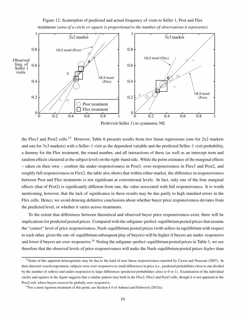
Figure 12: Scatterplots of predicted and actual frequency of visits to Seller 1, Post and Flex
treatments (area of a circle or square is proportional to the number of observations it represents)
��
��
��
��
��
��
��
��
��
��
��
��
��
��
��
��
��
��
��
��
Prob(visit Seller 1) in symmetric NE
Observedfreq. ofSeller 1visits
0 00.2 0.20.4 0.40.6 0.60.8 0.81 1
1 1
0.8 0.8
0.6 0.6
0.4 0.4
0.2 0.2
0 0
2x2 market 3x3 market
iPost treatment
Flex treatmentpppppppppppppppppppppppppppppppppppppppppppppppppppppppppppppppppppppppppppppppppppppppppppppppppppppppp
pppppppppppppp
pppppppppppppp
pppppppppppppp
pppppppppppppp
pppppppppppppp
pppppppppppppp
pppppppppppppp
pppppppppppppp
pppppppppppppp
pppppppppppppp
pppppppppppppppppppppppppppppppppppppppppppppppppppppppppppppppppppp
p p p p p p p p pp p p p p p p p p
p p p p p p p p pp p p p p p p p p
p p p p p p p p pp p p p p p p p p
p p p p p p p p pp p p p p p p p p
p p p p p p p p pp p p
OLS trend (Post)���:
OLS trend(Flex)
CCCCCO OLS trend (Flex)
QQs
OLS trend(Post)
CCCCCO
a
b d
� ��
h� ��
d
a a
a c f m� ��k
a
e
a a
the Flex3 and Post2 cells.15 However, Table 6 presents results from two linear regressions (one for 2x2 markets
and one for 3x3 markets) with a Seller–1 visit as the dependent variable and the predicted Seller–1 visit probability,
a dummy for the Flex treatment, the round number, and all interactions of these (as well as an intercept term and
random effects clustered at the subject level) on the right–hand side. While the point estimates of the marginal effects
– taken on their own – confirm the under–responsiveness in Post3, over–responsiveness in Flex3 and Post2, and
roughly full responsiveness in Flex2, the table also shows that within either market, the difference in responsiveness
between Post and Flex treatments is not significant at conventional levels. In fact, only one of the four marginal
effects (that of Post2) is significantly different from one, the value associated with full responsiveness. It is worth
mentioning, however, that the lack of significance in these results may be due partly to high standard errors in the
Flex cells. Hence, we avoid drawing definitive conclusions about whether buyer price responsiveness deviates from
the predicted level, or whether it varies across treatments.
To the extent that differences between theoretical and observed buyer price responsiveness exist, there will be
implications for predicted posted prices. Compared with the subgame–perfect–equilibriumposted prices that assume
the “correct” level of price responsiveness, Nash–equilibrium posted prices (with sellers in equilibrium with respect
to each other, given the out–of–equilibrium subsequent play of buyers) will be higher if buyers are under–responsive
and lower if buyers are over–responsive.16 Noting the subgame–perfect–equilibrium posted prices in Table 1, we see
therefore that the observed levels of price responsiveness will make the Nash–equilibrium posted prices higher than
15Some of this apparent heterogeneity may be due to the kind of non–linear responsiveness reported by Cason and Noussair (2007). In
their directed–search experiment, subjects were over–responsive to small differences in price (i.e., predicted probabilities close to one divided
by the number of sellers) and under–responsive to large differences (predicted probabilities close to 0 or 1). Examination of the individual
circles and squares in the figure suggests that a similar pattern may hold in the Flex2, Flex3 and Post3 cells, though it is not apparent in the
Post2 cell, where buyers seem to be globally over–responsive.16For a more rigorous treatment of this point, see Section 4.4 of Anbarci and Feltovich (2015a).
19

Table 6: Linear probability regressions, buyer visits to Seller 1
(average marginal effects, with standard errors in parentheses)
[17] [18]
Market 2x2 3x3
Predicted visit probability... 1.575∗∗∗ 1.427∗∗
(0.459) (0.671)
...under posting 2.075∗∗∗ 0.749∗∗∗
(0.431) (0.265)
...under flexible pricing 1.169 1.912∗
(0.754) (1.134)
Signif. diff. from each other? p ≈ 0.30 p ≈ 0.32
Flex treatment 0.003 0.003
(0.031) (0.026)
Round –0.001 0.001
(0.001) (0.001)
N 2320 2880
R2 0.045 0.023
* (**,***): Marginal effect significantly different from
zero at the 10% (5%, 1%) level.
9.33 in the Post3 cell, lower than 6.67 in the Flex3 cell, and lower than 10.00 in the Post2 cell, while not appreciably
changing the prediction of 10.00 or higher for the Flex2 cell. Hence, the subgame–perfect–equilibrium prediction
for the 3x3 market of higher posted prices under posting than under flexible prices is amplified by buyers’ actual
price responsiveness, while in the 2x2 market, buyer behaviour implies lower Nash–equilibrium prices under posting
than under flexible prices, whereas there need not have been a difference in the subgame–perfect–equilibrium prices.
So, while out–of–equilibrium visit behaviour by buyers may partly explain the higher posted prices observed in the
Post3 cell than in the Flex3 cell, it cannot do the same for the corresponding cells in the 2x2 market.
There are a few more minor aspects of buyer visit behaviour that deviate from the assumptions we made in
solving the theoretical model. Under flexible pricing, we had assumed that buyers should be indifferent between
sellers if posted prices are above 10, since at any such price, the buyer will get 10 if he is the only visitor to the
seller, or 0 if he is one of multiple visitors. However, even at these posted prices, buyers are price–responsive. In
the 2x2 market, they visit the lower–priced seller 58.6 percent of the time (instead of the predicted 50 percent) when
the two posted prices differ and both are at least 10, while in the 3x3 market, they visit the lowest–priced seller 42.1
percent of the time (instead of the predicted 33.3 percent) when there is a unique lowest price and all three prices are
at least 10.17 We even see some biases in the Hagg treatment, where even though no prices are posted, buyers can
potentially use the labels given to sellers in determining their visit choices. They appear not to do this systematically
in the 2x2 market – visiting Seller 1 and Seller 2 with frequency 49.4 and 50.6 percent respectively – but in the
17Of course, while such buyer behaviour is at odds with the assumption we had made in Section 2.1, it is sensible given the actual
relationships between posted and transaction prices seen in Section 4.1. Note also that this behaviour in the Flex treatment – with different
price pairs implying the same theoretical visit probabilities but different observed visit frequencies – is consistent with, and perhaps provides
an explanation for, the large standard errors for that treatment seen in Table 6.
20

3x3 market they seem to favour lower–numbered sellers somewhat, visiting Sellers 1, 2 and 3 with frequency 36.5,
32.6 and 30.8 percent respectively. Such favouritism cannot be exploited directly by sellers, who are not told their
numbers, but it does have a slight effect on local market thickness – deviations from uniform random choice increase
the likelihood of being one of multiple visitors to a seller at the expense of the likelihood of being the sole visitor.
5 Discussion
We have used theoretical analysis and a lab experiment to gain understanding of how the market institution affects
market outcomes. We have examined three institutions: price posting both with and without subsequent negotiation
(“flexible pricing” and “posting”, respectively) and negotiation without prior posting (“haggling”). The character-
istics of the good being traded, those of buyers and sellers, and global market thickness are held constant, enabling
us to isolate the effect of the institution itself without many of the confounds that would be present in the field. To
our knowledge, this is the first attempt to compare market institutions under controlled conditions, and also the first
controlled study of price posting with subsequent negotiation (our flexible–pricing treatment).
The results of the experiment support an “as–if” characterisation of rational market behaviour. We find many
examples of deviations from theoretical predictions in individual stages of each experimental cell. In the auction
stage under haggling and flexible pricing, buyers capture a non–negligible share of the surplus (as compared to
the prediction of all surplus going to sellers), even though it is publicly announced that all buyers have the same
valuation. In the bargaining stage under flexible pricing, sellers capture nearly all the available surplus conditional
on agreement, irrespective of the original posted price; this is in contrast to the prediction of multiple bargaining
solutions of an equal split when the posted price favours the seller. And under posting and flexible pricing, buyers’
price responsiveness varies substantially, with over–responsiveness in some cells and under–responsiveness in others.
Despite these deviations, the theoretical predictions for market–level qualitative comparisons (see Section 2.1)
are typically confirmed in the experiment.
1. As predicted, average transaction prices and seller profit in the 3x3 markets were lowest under posting and
highest under haggling, while buyer profit showed the opposite ordering. Correspondingly, buyer profit was
highest under posting and lowest under haggling in both markets.
2. In the 2x2 markets, transaction prices were lower – and buyer profit was higher – under posting than under
haggling or flexible pricing, as predicted (though not all of these differences were significant).
3. While seller profit in 2x2 markets was higher (not lower as predicted) under posting than under flexible pricing,
and while the predicted higher seller profit under haggling than under posting was observed but not significant,
these results are attributable to a short–lived higher efficiency under posting than in the other two institutions,
which countervails the effect of the difference in transaction prices.
The differences we observe between posting without negotiation and prices determined by negotiation (either
haggling or flexible pricing) are, for the most part, consistent with the theoretical results from the bulk of the previous
literature discussed in Section 1. They also lend themselves to nice intuition. For a given posted price, flexible pricing
allows the seller to capture most of the surplus when visited by multiple buyers, while not having to discount too
much when visited by only one buyer, compared with selling at the posted price under non–negotiable posting. This
21

allows sellers under flexible pricing to lower their posted prices compared to non–negotiable posting, while still
averaging higher transaction prices.18
Haggling (without posted prices) presents sellers with a further advantage over flexible pricing. Both perform
similarly when multiple buyers visit, with the seller gaining most of the surplus. But when only one seller visits,
haggling without a previously posted price tends to lead to agreements slightly favouring the seller, while under
flexible pricing, the original posted price caps the amount sellers can receive. Since posted prices under flexible
pricing centre roughly on the equal–split price of $10, transaction prices conditional on one buyer visiting will be
somewhat lower than those corresponding prices under haggling, so that average transaction prices will be lower
under flexible pricing than under haggling.
While the focus of our paper is on the comparison of market institutions, the deviations from theory seen in
our bargaining and auction results deserve some additional comment. We view the deviations in the auction results
as being relatively minor: given that the theory implies a corner solution in this case (bidding equal to value, the
maximum allowable bid), so that only deviations in one direction from this solution were plausible (indeed, even
if the experiment had not prevented bidding above value, the substantial likelihood of incurring money losses from
bidding above value suggests that such bids would have been rare), average bids below the equilibrium prediction
should not be surprising. Moreover, even out of equilibrium, buyers face incentives to raise their bids, and this is
observed in an upward time trend (see Table 5 and footnote 12). Given this time trend, it is reasonable to expect that
with sufficient experience, near–equilibrium behaviour ought to be seen in the auction stage.
On the other hand, it is unlikely that the deal–me–out (or, equivalently, risk dominant, etc.) bargaining predic-
tion would have been observed in our flexible–pricing treatment, even with experienced subjects. As noted in the
discussion surrounding Table 4, there was no discernible time trend toward deal–me–out in the data. Even more
interesting is the way in which deal–me–out fails: not when the posted price is below the equal–split value of $10 so
that deal–me–out implies a transaction price equal to the posted price, but rather, when the posted price is above $10,
implying a deal–me–out transaction price of $10.19 Instead, transaction prices increase nearly one–for–one with the
posted price, which determines the maximum allowable transaction price, and this is true even for posted prices
well above $10. These bargaining outcomes are therefore not only inconsistent with deal–me–out, they are also
inconsistent with equal split. Given the near–universal tendency toward equal splits in bargaining experiments when
neither side is structurally favoured (see Anbarci and Feltovich, 2015b, for a survey), this particular finding is novel
and striking. At first glance, one might attribute the result to our labelling of bargainers as buyers and sellers, which
differs from the typical procedure in bargaining experiments of giving subjects either abstract labels (e.g., “player
1” and “player 2”) or none at all, and might be expected to lead to their bringing their outside–world experience in
buying and selling into the lab. However, the results from our haggling treatment, where the seller’s share of the
surplus is between 55 and 60 percent – more than half, but nowhere near the upper bound of 100 percent – suggest
that labelling per se only has a small effect. Rather, it seems as though when a price is posted, it provides a strong
18As the market size increases, the attraction of flexible versus fixed prices also increases. Conditional on being visited by at least one
buyer, the probability of being visited by multiple buyers in nxn markets (those with equal numbers of buyers and sellers) increases with n:
while only 0.5 in the 2x2 case and 0.58 in the 3x3 case, it is 0.68 when n = 10 and 0.70 when n = 20, and approaches (e−2) asymptotically.19When the posted price is below $10, even random deviations from the prediction can only go in one direction – below the prediction of
the posted price – so it would be reasonable to expect average transaction price to lie below the posted price. When the posted price is above
$10, deviations in both directions from the prediction of $10 are possible, so random errors would tend to cancel out. However, as seen in
Figure 10, transaction prices tend to be close to the posted price.
22

focal point that swamps other plausible focal points – not only deal–me–out and equal–split, but also others such as
split–the–difference (which would imply a transaction price of half the posted price).20
We close by mentioning some of the limitations of this study; these will imply directions for future extensions.
First, the homogeneous–agent assumption we have made is a strong one. If there is dispersion in buyers’ valua-
tions and sellers’ costs, and these are private information, sellers’ benefit from haggling and flexible pricing may
decrease as disagreement rates in bargaining rise and less surplus is extracted in auctions, making posted pricing
more attractive. Posting would also become more attractive if a second assumption were relaxed: that of zero–cost
negotiating (ignoring foregone time, for example). Perhaps most important is a third assumption: exogenous insti-
tutions. If each individual seller were able to choose not just a posted price, but the entire market institution she will
use (posted prices without negotiation, haggling, flexible prices, etc.), and buyers knew which institution each seller
chose before making their visit decisions, we could investigate not only the performance of each institution, but also
which ones thrive and which ones do not.21 This is a non–trivial question: based on our results, sellers would ceteris
paribus prefer haggling without posting prices, but a market with only haggling ought to be vulnerable to invasion
by price–posting sellers (whom buyers would prefer to visit).
References
Albrecht, James, Pieter Gautier, and Susan Vroman (2006), “Equilibrium directed search with multiple applica-
tions”, Review of Economic Studies 73, pp. 869–891.
Anbarci, Nejat, Richard Dutu and Nick Feltovich (2015), “Inflation tax in the lab: a theoretical and experimental
study of competitive search equilibrium with inflation”, Journal of Economic Dynamics and Control 61, pp.
17–33.
Anbarci, Nejat and Nick Feltovich (2013), “Directed search, coordination failure and seller profits: an experimental
comparison of posted pricing with single and multiple prices”, International Economic Review 54, pp. 873–
884.
Anbarci, Nejat and Nick Feltovich (2015a), “Pricing in competitive search markets: experimental evidence of the
roles of price information and fairness perceptions”, working paper, Monash University.
Anbarci, Nejat and Nick Feltovich (2015b), “How fully do people exploit their bargaining position? The effects of
bargaining institution and the 50–50 norm”, working paper, Monash University.
Binmore, Ken, Chris Proulx, Larry Samuelson and Joe Swierzbinski (1998), “Hard bargains and lost opportunities”,
Economic Journal 108, pp. 1279–1298.
Binmore, Ken, Avner Shaked and John Sutton (1989), “An outside option experiment”, Quarterly Journal of Eco-
nomics 104, pp. 753–770.
Burdett, Kenneth, Shouyong Shi and Randall Wright (2001), “Pricing and matching with frictions”, Journal of
Political Economy 109, pp. 1060–1085.
20The only similar result we know of is that of Holm and Runnemark, 2014.21See Geromichalos, 2012, for a theoretical treatment of this topic.
23

Camera, Gabriele and Cemil Selcuk (2009), “Price dispersion with directed search”, Journal of the European
Economic Association 7, pp. 1193–1224.
Carlsson, Hans (1991), “A bargaining model where parties make errors”, Econometrica 59, pp. 1487–1496.
Case, Karl E. and Robert J. Shiller (2003), “Is there a bubble in the housing market?” Brookings Papers on
Economic Activity 34, pp. 299–362.
Cason, Timothy N. and Charles Noussair (2007), “A market with frictions in the matching process: an experimental
study”, International Economic Review 48, pp. 665–691.
Eckel, Catherine C. and Phillip J. Grossman (2008), “Forecasting risk attitudes: an experimental study of actual
and forecast risk attitudes of women and men”, Journal of Economic Behavior & Organization 68, pp. 1–17.
Fischbacher, Urs (2007), “z–Tree: Zurich toolbox for ready–made economic experiments”, Experimental Eco-
nomics 10, pp. 171–178.
Geromichalos, Athanasios (2012), “Directed search and optimal production”, Journal of Economic Theory 147,
pp. 2303–2331.
Greiner, Ben (2015), “Subject pool recruitment procedures: organizing experiments with ORSEE”, Journal of the
Economic Science Association 1, pp. 114–125.
Han, Lu and William C. Strange (2014), “What is the role of the asking price for a house?” Working paper,
University of Toronto.
Helland, Leif, Espen Moen and Edgar Preugschat (2014), “Information and coordination frictions in experimental
posted offer markets”, working paper.
Holm, Hakan and Emma Runnemark (2014), “Equal splits or reference prices: behavioral differences in focal point
selection”, working paper, Lund University.
Julien, Benoit, John Kennes, and Ian P. King (2000), “Bidding for labor”, Review of Economic Dynamics 3, pp.
619–649.
Julien, Benoit, John Kennes, and Ian P. King (2001), “Auctions and posted prices in directed search equilibrium”,
Topics in Macroeconomics 1, Article 1.
Julien, Benoit, John Kennes, and Ian P. King (2002), “Auctions beat posted prices in a small market”, Journal of
Institutional and Theoretical Economics 158, pp. 548–562.
Kloosterman, Andrew (2016), “Directed search with heterogeneous firms: an experimental study”, Experimental
Economics 19, pp. 51–66.
Kultti, Klaus (1999), “Equivalence of auctions and posted prices”, Games and Economic Behavior 27, pp. 106–
113.
Lagos, Ricardo and Randall Wright (2005), “A unified framework for monetary theory and policy analysis”, Journal
of Political Economy 113, pp. 463–484.
24

Lester, Benjamin (2011), “Information and prices with capacity constraints”, American Economic Review 101, pp.
1591–1600.
Lu, Xiaohua and R. Preston McAfee, August 1996, “The evolutionary stability of auctions over bargaining”, Games
and Economic Behavior 15, pp. 228–254.
McKelvey, Richard D., McLennan, Andrew M. and Turocy, Theodore L. (2014), “Gambit: software tools for game
theory”, version 13.1.2, www.gambit-project.org.
Milgrom, Paul R. and Robert J. Weber (1982), “A theory of auctions and competitive bidding”, Econometrica 50,
pp. 1089–1122.
Moen, Espen R. (1997), “Competitive search equilibrium”, Journal of Political Economy 105, pp. 385–411.
Nash, John (1950), “The bargaining problem”, Econometrica 18, pp. 155–162.
Nash, John (1953), “Two–person cooperative games”, Econometrica 21, pp. 128–140.
Peters, Michael (1991), “Ex–ante price offers in matching games non–steady states”, Econometrica 59, pp. 1425–
1454.
Scull, Penrose and Prescott C. Fuller (1967), From Peddlers to Merchant Princes: a History of Selling in America.
Follett, Chicago.
Shimer, Robert (1996), “Contracts in frictional labor markets”, working paper, MIT.
Siegel, Sidney and N. James Castellan, Jr. (1988), Nonparametric Statistics for the Behavioral Sciences, McGraw–
Hill, New York.
Smith, Adam (1776), An Inquiry into the Nature and Causes of the Wealth of Nations, 1st ed., London, W. Strahan.
Stacey, Derek (2015), “Posted prices, search and bargaining”, working paper, Ryerson University.
Sutton, John (1986), “Non–cooperative bargaining theory: an introduction”, Review of Economic Studies 53, pp.
709–724.
25

Appendix A: Experiment instructions
Below is the text of the instructions used in the experiment. Text that differed across treatments is placed inside square brackets, along with the relevant treatment (this was not in the original instructions). Part 2 was the same in all three treatments.
Instructions (Part 1)
You are about to participate in a decision making experiment. Please read these instructions carefully, as the money you earn may depend on how well you understand them. If you have a question at any time, please feel free to ask the experimenter. We ask that you not talk with the other participants during the experiment, and that you put away your mobile phones and other devices at this time.
This experiment has two parts. These instructions are for Part 1; you will receive new instructions after this part has finished. Part 1 is made up of 40 rounds, each consisting of a simple computerised market game. Before the first round, you are assigned a role: buyer or seller. You will remain in the same role throughout the experiment.
In each round, the participants in this session are divided into “markets”. A market is either a group of 4 containing a total of 2 buyers and 2 sellers, or a group of 6 containing 3 buyers and 3 sellers. The other people in your market will be randomly assigned in each round. You will not be told the identity of the people in your market, nor will they be told yours – even after the session ends.
The market game: In each round, a seller can produce one unit of a hypothetical good, at a cost of $0. A buyer can buy up to one unit of the good, which is resold to the experimenter at the end of the round for $20. It is not possible to buy or sell more than one unit in a round. [Post: A round begins with sellers choosing their prices, which are entered as multiples of 0.10, between 0 and 20 inclusive (without the dollar sign). After sellers have chosen their prices, the buyers are told the prices of each of the sellers in their market, and then each buyer chooses which seller to visit. A seller might be visited by zero, one, or more than one buyers. Any seller visited by zero buyers is unable to sell in that round. If exactly one buyer visits a particular seller, then that buyer pays the seller’s price for the seller’s item. If more than one buyer visits the same seller, then since the seller only has one unit, one of the buyers is randomly selected by the computer to purchase it at that seller’s price, and the other buyers are unable to buy.] [Hagg: A round begins with buyers choosing which seller to visit. A seller might be visited by zero, one, or more than one buyers. Any seller visited by zero buyers is unable to sell in that round. If exactly one buyer visits a particular seller, then the buyer and seller negotiate over the final price. The seller chooses an offer price, and the buyer chooses a bid price. Both of these can be any multiple of 0.10, between 0 and 20 inclusive. - If the buyer’s bid price is greater than or equal to the seller’s offer price, then the buyer and seller trade, and the final price is equal to the average of the bid and offer prices ( [bid price + offer price] / 2 ). - If the buyer’s bid price is less than the seller’s offer price, then they do not trade in that round: the buyer doesn’t buy and the seller doesn’t sell. If more than one buyer visits the same seller, then since the seller only has one unit, the unit is auctioned

off to determine which buyer is able to buy. The seller chooses a reserve price, and each buyer chooses a bid price. These can be any multiple of 0.10, between 0 and 20.00 inclusive. - If one or more bids are greater than or equal to the seller’s reserve price, then the seller sells to the buyer with the highest bid (any ties are broken randomly by the computer), and the final price is equal to either the second-highest bid or the reserve price, whichever is larger. The other buyers visiting that seller are unable to buy in that round. - If all of the bids are less than the seller’s reserve price, then they do not trade in that round: the buyers don’t buy and the seller doesn’t sell.] [Flex: A round begins with sellers choosing their prices, which are entered as multiples of 0.10, between 0 and 20 inclusive (without the dollar sign). After sellers have chosen their prices, the buyers are told the prices of each of the sellers in their market, and then each buyer chooses which seller to visit. A seller might be visited by zero, one, or more than one buyers. Any seller visited by zero buyers is unable to sell in that round. If exactly one buyer visits a particular seller, then the buyer and seller negotiate over the final price. The seller chooses an offer price, and the buyer chooses a bid price. These can be any multiple of 0.10, between 0 and the seller’s original price inclusive. - If the buyer’s bid price is greater than or equal to the seller’s offer price, then the buyer and seller trade, and the final price is equal to the average of the bid and offer prices ( [bid price + offer price] / 2 ). - If the buyer’s bid price is less than the seller’s offer price, then they do not trade in that round: the buyer doesn’t buy and the seller doesn’t sell. If more than one buyer visits the same seller, then since the seller only has one unit, the unit is auctioned off to determine which buyer is able to buy. The seller chooses a reserve price, and each buyer chooses a bid price. Both of these can be any multiple of 0.10, between the seller’s original price and 20.00 inclusive. - If one or more bids are greater than or equal to the seller’s reserve price, then the seller sells to the buyer with the highest bid (any ties are broken randomly by the computer), and the final price is equal to either the second-highest bid or the reserve price, whichever is larger. The other buyers visiting that seller are unable to buy in that round. - If all of the bids are less than the seller’s reserve price, then they do not trade in that round: the buyers don’t buy and the seller doesn’t sell.] Profits: Your profit for the round depends on the round’s result. - If you are a seller and you are able to sell, your profit is the price you chose. - If you are a seller and you are unable to sell, your profit is zero. - If you are a buyer and you are able to buy, your profit is $20.00 minus the price you paid. - If you are a buyer and you are unable to buy, your profit is zero. Sequence of play in a round: [Post: (1) The computer randomly forms markets. You are reminded of how many buyers and sellers are in your
market, and whether you are a buyer or seller. (2) Sellers choose their prices. (3) Buyers observe the sellers’ prices, then each buyer chooses which seller to visit. (4) The round ends. You are informed of the results of your market, including each seller’s price, how
many buyers visited you (if you are a seller) or the same seller as you (if you are a buyer), the quantity you bought or sold, and your profit for the round.]

[Hagg: (1) The computer randomly forms markets. You are reminded of how many buyers and sellers are in your
market, and whether you are a buyer or seller. (2) Each buyer chooses which seller to visit. (3) If a seller is visited by exactly one buyer, they negotiate: the buyer chooses a bid price and the seller
chooses an offer price. If a seller is visited by more than one buyer, there is an auction: the buyers bid and the seller chooses a reserve price.
(4) The round ends. You are informed of the results of your market, including how many buyers visited you (if you are a seller) or the same seller as you (if you are a buyer), the quantity you bought or sold, and your profit for the round.]
[Flex: (1) The computer randomly forms markets. You are reminded of how many buyers and sellers are in your
market, and whether you are a buyer or seller. (2) Sellers choose their prices. (3) Buyers observe the sellers’ prices, then each buyer chooses which seller to visit. (4) If a seller is visited by exactly one buyer, they negotiate: the buyer chooses a bid price and the seller
chooses an offer price. If a seller is visited by more than one buyer, there is an auction: the buyers bid and the seller chooses a reserve price.
(5) The round ends. You are informed of the results of your market, including each seller’s price, how many buyers visited you (if you are a seller) or the same seller as you (if you are a buyer), the quantity you bought or sold, and your profit for the round.]
After this, you go on to the next round. Payments: Your payment depends on the results of the experiment. At the end of the experiment, four rounds from Part 1 will be chosen randomly for each participant. You will be paid the total of your profits from those selected rounds, plus whatever you earn in the remainder of the experiment. Payments are made privately and in cash at the end of the session.
Instructions (Part 2)
In this part of the experiment, you will begin by being shown five gambles, and choosing the one you prefer. Each gamble has two possible outcomes, with equal (50%) chance of occurring. The gambles are as follows:
Gamble Random numbers 1-50 (50% chance) Random numbers 51-100 (50% chance)
1 You earn $4 You earn $4
2 You earn $6 You earn $3
3 You earn $8 You earn $2
4 You earn $10 You earn $1
5 You earn $12 You earn $0

After you have chosen one of these gambles, the computer will randomly draw a whole number between 1 and 100 (inclusive). If the random number is 50 or less, your earnings from this task are as shown in the middle column of the table. If the random number is 51 or more, your earnings are given by the right column. The random number drawn for you may be different from the ones drawn for other participants. Once you have chosen a gamble, you will be shown another screen containing a questionnaire. You will receive an additional $10 for answering all of the questions. Once everyone has finished the questionnaire, you will be shown your results from this part and the previous part of the experiment.

Appendix B: Sample screenshots Seller price-posting choice:
Buyer visit choice:

Buyer bargaining stage:
Seller bargaining stage:

Buyer auction stage:
Seller auction stage:

Risky-choice task:
Questionnaire: