market demand estimation for new product development by using fuzzy modeling and discrete choice...

Author's Accepted Manuscript

Market demand estimation for new productdevelopment by using fuzzy modeling anddiscrete choice analysis

R. Aydin, C.K. Kwong, P. Ji, H.M.C. Law

PII: S0925-2312(14)00524-4DOI: http://dx.doi.org/10.1016/j.neucom.2014.01.051Reference: NEUCOM14125

To appear in: Neurocomputing

Received date: 17 September 2013Revised date: 2 January 2014Accepted date: 3 January 2014

Cite this article as: R. Aydin, C.K. Kwong, P. Ji, H.M.C. Law, Market demandestimation for new product development by using fuzzy modeling anddiscrete choice analysis, Neurocomputing, http://dx.doi.org/10.1016/j.neu-com.2014.01.051

This is a PDF file of an unedited manuscript that has been accepted forpublication. As a service to our customers we are providing this early version ofthe manuscript. The manuscript will undergo copyediting, typesetting, andreview of the resulting galley proof before it is published in its final citable form.Please note that during the production process errors may be discovered whichcould affect the content, and all legal disclaimers that apply to the journalpertain.

www.elsevier.com/locate/neucom

http://dx.doi.org/10.1016/j.neucom.2014.01.051







Market demand estimation for new product development by using fuzzy

modeling and discrete choice analysis

R. Aydina, C.K. Kwonga, P. Jia, H.M.C. Lawb

a Department of Industrial and Systems Engineering, The Hong Kong Polytechnic University, Hong Kong b G.E.W. International Corporation Limited, Hong Kong

Keywords: New product development; Discrete choice analysis; Conjoint analysis; Fuzzy

market demand model; Fuzzy regression; Uncertainty.

Abstract

Market demand estimation is an important process to assess the financial feasibility of new

product development (NPD) projects. The development of models for market demand

estimation involves market potential estimation and choice modeling. Previous studies

commonly used conjoint analysis to develop utility functions which were then used in

discrete choice models to generate market share models. The jury of executive opinion

method is commonly used in industries wherein a number of experts and/or consultants are

always involved in the market potential estimation. However, a high degree of fuzziness

always exists in the data obtained from conjoint surveys and the market potential estimation

because of the subjective judgments of respondents and experts. However, ignorance of the

fuzziness would lead to the over-estimation of market demands. This research aims to tackle

the fuzziness associated with market potential estimation and survey data in the development

of market demand models. In this paper, a new methodology of developing fuzzy market

demand models for NPD is proposed to address the fuzziness by which market demands can

be estimated for the worst, normal, and best scenarios. The proposed methodology involves

fuzzy choice modeling based on fuzzy regression and discrete choice analysis, and fuzzy

estimate generation of market potential. To evaluate the effectiveness of the proposed

methodology, a case study of market demand estimation of a new tablet PC is conducted

based on the proposed methodology. The results of the implementation are compared with

2��

those based on a popular multinominal logit (MNL) based demand model. From the

comparison, it can be noted that the estimated market demand based on the MNL model is

very close to that for the normal scenario based on the proposed fuzzy demand model.

However, the MNL model cannot provide estimates for other scenarios.

1. Introduction

Market demand estimation is widely used to assist companies in assessing the financial

feasibility of new product development (NPD) projects. Market demand estimation

commonly involves choice modeling and market potential estimation. Choice modeling [17]

is a common method used in the decision-making process to understand customer buying

behavior and preferences and measure tradeoffs among attributes in a given set of product

alternatives. Early choice modeling applications have been used to solve problems in the

travel, transportation, and tourism industries according to the principle of utility

maximization of customers. In the last decades, choice modeling has been widely applied in

marketing research [16]. In recent years, it has been used to associate consumer preferences

with design attributes for NPD [26]. Choice modeling has a number of applications in the

demand modeling of product design because of the necessity of integrating engineering

design attributes with marketing desired attributes. Choice modeling can capture consumer

preferences for a set of competitive products, thus making this approach suitable for

integrating marketing and engineering approaches in product design [1]. Choice modeling

outputs provide important information to decision makers in determining product features

and variables to satisfy customer expectations. The latest research in choice modeling aims to

understand heterogeneous consumer preferences, estimate market demand under competition

and/or uncertainty, and study uncertainties associated with customer purchasing behavior in

demand modeling [26].

3��

Discrete choice analysis (DCA) is a disaggregate approach to choice modeling that is

based on probabilistic distribution theory, which seeks the utility fraction of a given product

among a set of competitive products. DCA aims to maximize the total utility of individual

consumers who respond to experiments/surveys by capturing the tradeoffs among product

attributes. DCA uses preference data to estimate the choice probabilities of competing

alternatives for individual consumers. These individual estimations are then aggregated to

predict the total choice share. Various DCA models, such as multinomial logit (MNL) [1, 21],

nested logit [8] and mixed logit (MXL) [4, 26], have been applied in the demand modeling.

Conjoint analysis is a popular technique for capturing consumer preferences and

measuring tradeoffs by estimating the consumer part-worth utilities for each attribute level of

a product. Conjoint analysis can be used to generate the utility functions of products and

determine the optimum setting of product attributes by using the collected data of conjoint

surveys. Various types of conjoint analysis such as rankings, ratings, and choice-based

alternatives exist [1]. Conjoint analysis and DCA have been successfully applied to develop

market share models for new products [9, 10]. Market potential estimations are combined

with the generated market share models to develop market demand models. The jury of

executive opinion method [2], wherein several experts are involved in the estimation, is

commonly used in industries to estimate market potential for new products. However,

marketing experts estimate market potential mainly based on their own subjective judgments

and their estimates are always ambiguous such as ‘somehow about 80 thousands’, and ‘close

to 95 thousands’. As described by Kosko [7], fuzziness is "event ambiguity" which indicates

the degree of occurring an event rather than randomness. Thus, estimates of market potential

based on the jury of expert opinion can contain a high degree of fuzziness.

Studies have been conducted to consider the uncertainties in market demand estimation.

Uncertainties such as subjective responses in surveys data, dynamic market conditions, and

4��

rapid technological development can significantly affect the predictive accuracy of developed

market demand models. Therefore, the uncertainties should be considered in the development

of market demand models. Turksen et al. [27] developed a fuzzy set preference model to

solve the problem of linguistic variable ambiguity in demand modeling in which fuzzy set

was introduced to define subject ratings as linguistic ratings rather than numerical ratings,

which is applied on conjoint analysis. Given the vagueness of consumer preferences, Lau et

al. [11] extended the MNL model with switching regression techniques. Fuzzy part-worth

utilities were proposed under different crisp and fuzzy scenarios to determine an optimal

product line extension scheme, and estimate the market share by considering the uncertainty

in consumer preferences [14]. Resende et al. [21] applied the Delta method to consider the

uncertainty of choice model parameters in determining an optimal setting of product design

attributes because of the vagueness in profit and market share estimations.

Demand uncertainty is caused by preference dynamics, demand model misspecification,

choice context, and response variability. Xiong et al. [29] studied uncertainty in consumer

demand by integrating fuzzy set theory into demand modeling to solve a dynamic pricing

problem. Williams et al. [28] used multi-objective robust optimization approach to handle

uncertainty issues in the market share estimation of bundled products. Razu and Takai [20]

attempted to model uncertainty in market demand by estimating customer utility errors by

applying bootstrap and Monte Carlo simulation on choice-based conjoint analysis. Lemos et

al. [13] introduced the evolving fuzzy linear regression tree method to manage the risks and

uncertainties associated with the sales forecasting of petroleum products. Lin et al. [14]

studied the uncertainty of consumer preferences caused by poor awareness of new

technologies, which can lead to the fuzziness of market potential estimation.

Consumer survey data contains high degrees of fuzziness because customer responses

are subjective and imprecise. Although fuzziness in market share estimation was considered

5��

in previous studies, none of them addressed the fuzziness of survey data that was used to

develop market demand models. On the other hand, the jury of executive opinion method is

commonly used in industries to estimate market potential of new products. However, the

fuzziness of the estimation was not addressed as well in previous studies. In this paper, a

novel methodology of developing fuzzy market demand models is proposed to address the

fuzziness. In the proposed method, fuzzy regression is introduced into DCA to address the

fuzziness of the survey data, and the fuzzy estimates of market potential are generated based

on the jury of executive opinion method to address the fuzziness of market potential

estimation.

The rest of this paper is organized as follows. Section 2 describes the proposed

methodology of generating fuzzy market demand models for new products. The proposed

methodology involves conjoint survey design, fuzzy regression analysis, fuzzy market

potential estimation, generation of fuzzy demand models, and defuzzification method.

Section 3 presents a case study of generating a fuzzy demand model to estimate the market

demand of a new tablet PC based on the proposed methodology. Finally, conclusion and

future work are provided in Section 4.

2. Proposed methodology

To address the fuzziness of survey data, a fuzzy regression method is introduced into DCA to

develop choice models. Fuzzy estimates of market potential, which are represented as

triangular fuzzy numbers (TFNs), are generated by the jury of executive opinion method.

Figure 1 shows a flowchart of the proposed methodology for developing fuzzy market

demand models for NPD. First, a conjoint survey is conducted to collect customer

preferences on products. Survey respondents are classified into a number of segments by

using a K-means clustering technique. Thereafter, fuzzy regression is used to generate the

6��

fuzzy utility functions of individual segments. Fuzzy choice (or market share) models are

developed based on the developed fuzzy utility functions and MNL model of DCA. The

fuzzy estimates of market potential are generated based on the jury of executive opinion

method. Once the choice models are developed and the fuzzy estimates are obtained, fuzzy

market demand models can be developed. Finally, a defuzzification method is introduced to

estimate the market demand of new products.

7��

Figure 1. A methodology for developing fuzzy market demand models.

2.1. Conjoint survey design

Rating- [6, 15], ranking- [14], and choice-based [20] conjoint surveys are the three types of

conjoint survey designs. The rating-based conjoint survey is adopted in this research; this

type of survey is widely used in previous studies and requires a set of product profiles with

respect to pre-defined attributes and attribute levels [6]. Rating-based conjoint surveys are

commonly designed based on orthogonal arrays [16]. Consumers are then asked to rate the

product profiles. Survey data is analyzed to generate the following utility functions:

��

�

�

� ��

where �� represents the utility of the j-th product profile in the i-th segment, and �� is

the part-worth utility of the l-th level of the k-th attribute in the segment i. m and �� denotes

the number of attributes and number of attribute levels in the k-th attribute, respectively. �� is defined as a dummy variable that is equal to one if the l-th level of the k-th attribute is

chosen for the product profile j and zero if otherwise. Hence, the total number of dummy

variables is �� .

2.2. Fuzzy utility functions

In this paper, fuzzy linear regression is used to estimate the coefficients of fuzzy utility

functions. The independent variables are the levels of product attributes, whereas the

dependent variables are the ratings of respondents on the product profiles obtained from

surveys. To generate the utility functions, dummy variables are introduced. To improve the

modeling of the preferences of heterogeneous customers, individual rating data is used to

8��

generate individual fuzzy utility functions, that is, a unique fuzzy utility function is generated

for each customer.

Given that human judgment and predictions are involved in the data set, uncertainty

occurs in a system with respect to the relationship between dependent and independent

variables. Tanaka et al. [25] developed a fuzzy linear regression model as an extension of

statistical linear regression analysis by relaxing the strict assumption of statistical models

regarding possibility distributions rather than probabilistic distributions [19]. The

fundamental difference between statistical regression models and fuzzy regression models is

the deviations between the observed and estimated values [23]. In statistical regression, data

variation is explained in terms of an estimated variance of measurement errors, whereas fuzzy

regression variation hinges on the vagueness or impreciseness of the system structure.

Therefore, fuzzy coefficients are determined by these deviations. Fuzzy regression models

can be applied to find the relationship between dependent and independent variables which is

denoted by a fuzzy function [19, 23]. The parameters are commonly denoted by fuzzy

numbers [5]. A fuzzy regression model can be expressed as follows:

�� , j=1,2,...,n, (2)

where �� is the estimated fuzzy output, �� is the fuzzy coefficient of the j-th independent

variable, and � is the non-fuzzy vector of the j-th inputs (independent variable). Fuzzy

coefficients are commonly expressed as TFNs, which can be either symmetric or asymmetric

[24].

The upper and lower intervals of a fuzzy linear regression model are constructed based

on outliers, and model generation depends on the interval estimation (Figure 2).

9��

Figure 2. Fuzzy regression intervals [22].

For symmetrical TFNs ��, the membership functions of �� !�� "�� can be expressed

as follows:

#$%&'(�) �� 1 *+,�-�.,*

/, , !� � "� 0 (� 0 !� � "� (3)

0, otherwise,

where !� is the center value of fuzzy number, and "� is the spread value of the fuzzy

number. Thereafter, a fuzzy linear regression function can be written as follows:

�� !�� "�� !�� "�� !�� "�� !�� "��. (4)

Thus, the membership function can be written as follows:

1 *1�-�23+*/3424 , 5 6

#7��8� � 1, � 6, 8 � 6 (5)

0, � 6, 8 5 6,

where 44 � �4�4� 9 � 4�4�:, :! is the central value of �� , ":44 is the spread value, and

#7��8��= 0 when ":44 0 48; ��:!4.

10��

Tanaka et al. [25] determined the objective function as minimizing the total spread of

the fuzzy coefficients. The purpose of the following model is to determine the central and

spread values of the coefficients with respect to the intervals supported by the h value.

<=�� "��>

� ��?��

which is subject to

� !�� @�� "�*��*>

� �

>

� �A �8BC � �� @�D��E��

� !�� @�� "�*��*>

� �

>

� �F �8BC � �� @�D��G�

"� A 6, �� , �H I, (9)

0�F �@� F �, = � ��J� 9 � <, K � 6� �� J� 9 � L,

where 8BC is the central value, and D� is the spread value of the i-th observed fuzzy data; !�

and "� are the center and spread values of the fuzzy coefficient of the j-th independent

variables respectively; �� is the variable for the j-th independent variable of the i-th

experimental data set. M is the number of experiment data sets, and N is the number of

independent variables. Eqs. (7) and (8) set the upper and lower boundaries of the estimated

data, respectively.

The h value is used to extend the supports of the membership function (confidence

interval) (Figure 3), which is defined as the degree of fitting of the fuzzy linear model. The

increase in h value leads to a decrease in the spread values of fuzzy coefficients.

11��

Figure 3. Supports of membership function with h value [22].

Tanaka et al. [24] revised the objective function of the fuzzy linear regression model as

minimizing the total fuzziness of the regression model by minimizing the total support of the

fuzzy outputs:

<=�� M"� �� *��*N

� �O

>

� �P��6��

2.3. Fuzzy estimates of market potential

Dalrymple [2] discussed the different types of sales forecasting methods, such as subjective,

extrapolation, and quantitative sales forecasting methods, used by companies in terms of

usage intention, effectiveness, and accuracy. The survey results indicate that the jury of

executive opinion (subjective), sales force composite (subjective), and naive methods are the

most common forecasting methods used in the industry.

The jury of executive opinion, which is also known as “expert judgment,” involves a

collection of forecasts/estimations from a number of executives, experts, and/or consultants.

The estimations are always subjective. The final estimation is determined by using simple

average and weighted average methods. To address the fuzziness of market potential

12��

estimation by the jury of executive opinion method, the fuzzy estimates of market potential

represented as TFNs are introduced. A fuzzy estimate of the market potential of market

segment i, <Q& �, can be expressed as �R�� !�� S��, where !� is the center value of the market

potential of the market segment i; R� and S� are the left and right spread values, respectively.

!� denotes the mean value of the market potential of market segment i estimated by

marketing executives or consultants:

!� � �T � !��

� ��

where !�� is the market potential of segment i estimated by the k-th marketing personnel. R� and S� can be determined by using Eqs. (12) and (13), respectively.

R� � !� � UVW� ��X�� !�� J��

S� � UYZ� ��X�� !�� !��[�� First, data on the market potential estimated by marketing executives and/or consultants

are collected. Second, the mean value of the fuzzy estimate of market potential is determined

by using Eq. (11). Finally, the spread values of the fuzzy estimate of market potential can be

determined by using Eqs. (12) and (13).

2.4. Development of fuzzy market demand models

Fuzzy market demand models can be developed by using the fuzzy estimates of market

potential and fuzzy choice models. In this section, the development of fuzzy choice models

based on the developed fuzzy utility functions and MNL model of DCA is described. The

development of fuzzy market demand models is also illustrated. The choice model in DCA is

built based on individual utility functions. DCA models include two main parts in the utility

13��

function, namely, a deterministic part U and a random disturbance �:

�\�� ]��, (14)

�� ^=�6 � �^=��K�� ^=��JK�J �� ^=�_RK_R, (15)

where �\�� represents the total utility of the j-th product profile for respondent n in

segment i, �� is the deterministic utility function of the observable independent variables

of the j-th product profile for respondent n in segment i, and ]�� is the random error of the

j-th product profile for respondent n in segment i. �̂�� is defined as the alternative-specific

constant for respondent n in segment i to capture the average effect of all unobserved factors

on the utility function. �̂�� is the utility coefficient of the l-th level of the k-th attribute for

respondent n in segment i, and �� is the dummy variable of the l-th level of the k-th

attribute for product profile j. �� equals to one if the l-th level of the k-th attribute is chosen

for the product profile j; otherwise, �� is zero [26].

All model coefficients (^s) are assumed identical across all respondents and are linear

within the observed (deterministic) part of the utility function. Random error terms � are

combined with the systematic part of the choice models by considering unobserved factors in

choice decisions. Random error terms are assumed independent and identically distributed

(IID) across respondent choices that reduce computation difficulty. Stochastic distribution is

assigned to estimate the unmeasured or unobserved behavior of the sampled group according

to assumptions made by decision makers [1].

Independence from irrelevant alternatives (IIA), which is one of the main properties of

the choice probabilities of DCA, implies that the ratio of the probabilities of choosing one

alternative over another one is independent of the choice set. IIA fundamentally brings

14��

proportional substitution among alternatives and ignores the correlation among alternatives;

thus, the introduction or exclusion of an alternative will result in an equal percent decrease or

increase in the choice probabilities of all other alternatives in the choice set. This property

provides a computational advantage in terms of adding or extracting alternatives in a choice

set [26]. The IIA property assumes that error terms are IID for the extreme value type 1 (EV1)

distribution, which is also called Gumbel or double-exponential distribution [16]. The mean

and variance of an EV1 distributed random variable are stated as <D(� � ` � 6PaEE# and

bYcVYWde � fgh #i, where ` is the mode parameter, and 1/# is the scale parameter. After a

series of derivations and integrations of the EV1 distribution regarding error terms, as well as

the formulation of pure closed-form MNL model, the estimate of the probability of choosing

the p-th product among the company's existing and competitive products by respondent n in

segment i denoted by QS��j� can be obtained as follows [1]:

QS��j� � Dklmn� Dklm,o� � �� Dklm�� Dklmn ��?�

where ��p is the utility of the p-th product for respondent n in segment i, and �� is the

utility of the k-th company's existing product for respondent n in segment i, and �� is the

utility of the j-th competitive product for respondent n in segment i.

After introducing the developed fuzzy utility functions into the MNL model, a fuzzy

choice model can be obtained and expressed as follows:

QS&��j� � Dkqlmn� Dkqlm,o� � �� Dkqlm�� Dkqlmn ��E�

where QS&��j� is the fuzzy probability of choosing the p-th product among the company's

existing and competitive products by respondent n in segment i, �q��p is the fuzzy utility of

15��

the p-th product for respondent n in segment i, �q�� is the fuzzy utility of the k-th company's

existing product for respondent n in segment i, and �q�� is the fuzzy utility of the j-th

competitive product for respondent n in segment i.

Hence, a fuzzy market demand model can be obtained as follows:

<r& �p � Dkqln� Dkql,o� � �� Dkql�� Dkqln ��R�� !�� S��G�

where <r& �p is the fuzzy market demand of the p-th product in segment i, �q�p is the fuzzy

utility of the p-th product in segment i, �q�� is the fuzzy utility of the j-th competitive product

in segment i, and �q�� is the fuzzy utility of the k-th company's existing product in segment i.

The worst, normal and best scenarios of market demand can be estimated by the

developed fuzzy market demand models via Eqs. (19), (20), and (21), respectively:

<r& �ps � tc��j��s��<Q& � � Dklnu

� Dkl,vo� � � � Dkl�v�� Dklnu ��R�� !�� S��w�

<r& �p� � tc��j��<Q& � � Dklnm

� Dkl,mo� � � � Dkl�m�� Dklnm ��R�� !�� S��J6�

<r& �px � tc��j��x��<Q& � � Dklnv

� Dkl,uo� � � � Dkl�u�� Dklnv ��R�� !�� S��J��

where <r& �ps , <r& �p� , and <r& �px are the fuzzy market demand of the p-th product in segment

i for the worst, normal, and best scenarios, respectively. tc��j��s, tc��j��, and tc��j��x are

the probability of choosing the p-th product in segment i for the worst, normal, and best

scenarios, respectively. ��ps, ��p� , and ��px are the utility of the p-th product in segment i for

16��

the worst, normal and best scenarios, respectively. ��s, �� , and ��x are the utility of the

j-th competitive product in segment i for the worst, normal and best scenarios, respectively.

��s, �� , and ��x are the utility of the k-th company's existing product in segment i for the

worst, normal, and best scenarios, respectively.

2.5. Estimation of market demand for new products by using centroid defuzzification

method

After fuzzy market demand models for a new product are generated, market demands of the

new product in the fuzzy number can be estimated corresponding to the worst, normal, and

best scenarios. To obtain the crisp estimated values of the market demand, a centroid

defuzzification method is adopted as follows [12]:

y � z #$��{x.z #$��{x.��JJ�

where y denotes the defuzzification (crisp) value; a and b are the minimum and maximum

values of x, respectively.

3.�Case�study�

A case study of the market demand estimation of a new tablet PC on the proposed

methodology is presented to illustrate the applicability and evaluate the effectiveness of the

proposed methodology. A computer product manufacturer is planning to develop a new tablet

PC for a particular market. Eight important product attributes were defined based on market

information and a lead user survey. To design a conjoint survey, the company also defined the

levels and their settings for individual attributes. Table 1 shows the eight product attributes

and their corresponding levels The green index was considered because of the increasing

17��

environmental concerns of consumers in the market. Green index “1” denotes that the

materials and components used for producing the products are new. Green index “2” implies

that 30% of the materials used in product manufacture are recycled and the price of the

product is 15% cheaper than that of the products with green index “1.” Green index “3”

indicates that 50% of the materials used in product manufacture are recycled and the price of

the products is 25% cheaper than that of the products with green index “1.”

Table 1. Product attributes and attribute levels of tablet PCs�

Index Attributes Attribute levels 1 CPU (Processor) 1/1.4/1.8 GHz 2 Memory (RAM) 512 MB/1 GB/2 GB 3 Hard Disk 16/32/64 GB 4 Screen Size 7/10 in 5 Screen Resolution 1024×768/1280×800/2048×1536 6 Battery Life 8/10/12 hrs 7 Connectivity Wi-Fi/Wi-Fi + 3G/Wi-Fi + 4 G 8 Green Index 1/2/3

Design of the survey and generation of product profiles for the survey is based on a L18

orthogonal array [18]. Table 2 shows a part of the survey questionnaire in which eighteen

product profiles are generated. The conjoint survey was conducted in a university. All the

respondents are university students with their early 20s and they are all experienced users of

tablet PCs. The students were invited to assess the eighteen product profiles by filling out the

survey questionnaires using the scales “1” to “5” which denote the linguistic variables, ‘very

bad’, ‘bad’, ‘moderate’, ‘good’ and ‘very good’, respectively. About 48% of the respondents

are female. Some outliers were noted and they were removed from the data sets which are for

the data analysis and modeling.

18��

Table 2. A survey questionnaire for tablet PCs

Once the survey data was collected, K-means clustering technique based on SPSS

software package was employed to identify consumer segments. In this case study, two

segments were identified. Thereafter, the ratings were converted to TFNs where the neighbor

functions intersect at the membership value of 0.5. Thus, when the membership value of a

function is “1,” the membership value of neighbor function(s) is “0” or vice versa. Figure 4

shows the membership functions of the linguistic variable used in the survey. Thus, the

ratings of “1” to “5” are converted into TFNs as follows:

“1” (very bad) = (0.83, 0.83); “2” (bad) = (1.67, 0.83); “3” (moderate) = (2.50, 0.83); “4”

(good) = (3.34, 0.83); “5” (very good) = (4.17, 0.83).

Attributes

Profiles CPU RAM Hard

Disk Screen Size

Screen Resolution

Battery Life Connectivity Green

Index Rating (1 – 5)

1 1 GHz 512 MB 16 GB 7 in 1024 × 768 8 hrs Wi-Fi 1

2 1 GHz 1 GB 32 GB 7 in 1280 × 800 10 hrs Wi-Fi + 3G 2

3 1 GHz 2 GB 64 GB 7 in 2048 × 1536 12 hrs Wi-Fi + 4G 3

4 1.4 GHz 512 MB 16 GB 7 in 1280 × 800 10 hrs Wi-Fi + 4G 3

5 1.4 GHz 1 GB 32 GB 7 in� 2048 × 1536 12 hrs Wi-Fi 1

6 1.4 GHz 2 GB 64 GB 7 in� 1024 × 768 8 hrs Wi-Fi + 3G 2

7 1.8 GHz 512 MB 32 GB 7 in� 1024 × 768 12 hrs Wi-Fi + 3G 3


9 1.8 GHz 2 GB 16 GB 7 in 2048 × 1536 10 hrs Wi-Fi 2

10 1 GHz 512 MB 64 GB 10 in� 2048 × 1536 10 hrs Wi-Fi + 3G 1

11 1 GHz 1 GB 16 GB 10 in� 1024 × 768 12 hrs Wi-Fi + 4G 2

12 1 GHz 2 GB 32 GB 10 in� 1280 × 800 8 hrs Wi-Fi 3

13 1.4 GHz 512 MB 32 GB 10 in� 2048 × 1536 8 hrs Wi-Fi + 4G 2

14 1.4 GHz 1 GB 64 GB 10 in� 1024 × 768 10 hrs Wi-Fi 3


16 1.8 GHz 512 MB 64 GB 10 in� 1280 × 800 12 hrs Wi-Fi 2



19��

�

Figure 4. Membership function for linguistic variables.

3.1. Development of fuzzy utility functions

In conjoint analysis, a dummy variable regression method is commonly used to generate

utility functions and the method is adopted in this research. In this case, each product

attribute consists of dummy variables for the attribute levels. If an attribute has _� levels, it

is coded in terms of _� � � dummy variables. Value of a dummy variable is either 1 or 0.

Taking the attribute CPU as an example, its levels were coded as follows.

�� i 1 GHz 1 0 1.4 GHz 0 1 1.8 GHz 0 0

Figure 5 shows the defined dummy variables and coded product profiles.

20��

Figure 5. Coded product profiles with dummy variables.

where �� and �i are the dummy variables for CPU; i� and ii are the dummy

variables for memory; |� and |i are the dummy variables for hard disk; } is a dummy

variable for screen size; ~� and ~i are the dummy variables for screen resolution; h�

and hi are the dummy variables for battery life; �� and �i are the dummy variables for

connectivity; �� and �i are the dummy variables for green index.

After defining the dummy variables and coding the product profiles, fuzzy regression

analysis was introduced to determine the fuzzy coefficients of the regression models. The

development of fuzzy utility functions was implemented using Matlab software. The fuzzy

utility functions for individual respondents in Segments 1 and 2 were generated. The

generated fuzzy utility functions for the first respondent of Segments 1 and 2 denoted as �q��

and �qi�, respectively, are shown as follows:

21��

�q�� P66� 6P6?� � �6P[a� 6�� 6P6E� 6Pa?��i � �6Paw� 6PJ��i� � �6Paw� 6PJ��ii� ��6P[G� 6PJ��|� � ��6P�� 6PJ��|i � �6P�� 6P��}�� 6P�� 6PJ��~� � ��6P[w� 6PJ��~i � �6P�E� 6PJ��h�� 6PJa� 6PJ��hi � ��JP[[� 6PJ�� P6G� 6PJ��i� �6Paw� 6PJ�� 6Paw� 6PJ��i��

�qi� � �aPE6� 6� � ��6PwG� �P[w�� PJa� 6PJG��i � �6P�� 6�i� � ��6PJG� 6�ii� ��6P�J� 6�|� � ��6Pa?� 6�|i � �6Pa?� 6�}� � ��6PG[� 6�~�� 6Paa� 6�~i � �6� 6�h� � ��6Pa?� 6�hi � ��6Pa?� 6�� 6P�J� 6��i � ��P?E� 6�� 6PwG� 6��i��

3.2. Market potential estimation of a new tablet PC

Five marketing executives were invited to estimate the market potential of the two segments.

Their estimations are shown in Table 3.

Table 3. Market potentials of two segments estimated by marketing executives

Marketing Executive Estimated Potential of Segment 1 (×1000)

Estimated Potential of Segment 2 (×1000)

A 76.8 163.2

B 83.2 176.8

C 90.2 191.8

D 84.8 180.2

E 89.6 190.4

The mean value of the fuzzy estimate of the market potential of Segment 1, !�, can be

determined using Eq. (11) as shown below.

!� � E?PG � G[PJ � w6PJ � G�PG � GwP?a � G�PwP

The left and right spread values of the fuzzy estimate are calculated as 8.1 and 5.3 by

22��

using Eqs. (12) and (13), respectively. Thus, <Q& � � �R�� !�� S�� GP�� G�Pw� aP[� . By

following the same procedures, the fuzzy estimate of the market potential of Segment 2, <Q& i,

were estimated as ��EP[� �G6Pa� ��P[�.

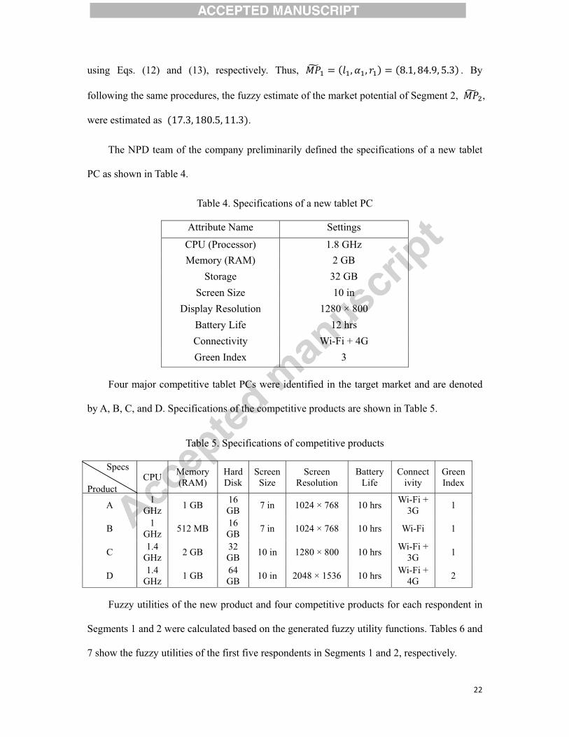
The NPD team of the company preliminarily defined the specifications of a new tablet

PC as shown in Table 4.

Table 4. Specifications of a new tablet PC

Attribute Name Settings

CPU (Processor) 1.8 GHz Memory (RAM) 2 GB

Storage 32 GB Screen Size 10 in

Display Resolution 1280 × 800 Battery Life 12 hrs Connectivity Wi-Fi + 4G Green Index 3

Four major competitive tablet PCs were identified in the target market and are denoted

by A, B, C, and D. Specifications of the competitive products are shown in Table 5.

Table 5. Specifications of competitive products

Fuzzy utilities of the new product and four competitive products for each respondent in

Segments 1 and 2 were calculated based on the generated fuzzy utility functions. Tables 6 and

7 show the fuzzy utilities of the first five respondents in Segments 1 and 2, respectively.

Specs Product

CPU Memory (RAM)

Hard Disk

Screen Size

Screen Resolution

Battery Life

Connectivity

Green Index

A 1 GHz 1 GB 16

GB 7 in 1024 × 768 10 hrs Wi-Fi + 3G 1

B 1 GHz 512 MB 16

GB 7 in 1024 × 768 10 hrs� Wi-Fi 1

C 1.4 GHz 2 GB 32

GB 10 in 1280 × 800� 10 hrs� Wi-Fi + 3G 1

D 1.4 GHz 1 GB 64

GB 10 in 2048 × 1536 10 hrs� Wi-Fi + 4G 2

23��

Table 6. Fuzzy utilities of the first five respondents in Segment 1

New A B C D

Center Spread Center Spread Center Spread Center Spread Center Spread

3.51 0.48 3.86 1.47 2.60 1.47 2.85 1.68 5.00 1.25 2.19 0.20 4.20 0.63 4.35 0.63 1.79 1.31 2.82 1.13 4.31 0.00 3.19 0.27 2.64 0.27 4.45 0.00 4.31 0.00 4.28 0.07 2.68 0.21 2.40 0.21 3.80 0.15 3.83 0.10 3.86 0.07 3.37 0.21 2.67 0.21 3.95 0.15 4.11 0.09

Table 7. Fuzzy utilities of the first five respondents in Segment 2

New A B C D

Center Spread Center Spread Center Spread Center Spread Center Spread

4.59 0.00 1.10 1.39 1.39 1.39 0.69 0.28 2.64 0.28

2.33 0.07 3.79 0.49 2.95 0.49 2.13 0.16 -0.06 0.10

3.47 0.00 1.52 0.83 1.10 0.83 2.50 0.00 2.64 0.00

3.33 0.00 1.39 0.28 0.83 0.28 5.28 0.28 3.20 0.28

4.97 0.07 2.81 0.21 2.54 0.21 2.83 0.16 2.30 0.10

The choice probabilities of individuals in Segments 1 and 2 for the worst, normal, and

best scenarios were calculated by using Eq. (17). Tables 8 and 9 show the choice probabilities

of the first five respondents in Segments 1 and 2, respectively.

Table 8. Choice probabilities of the first five respondents for Segment 1

Worst Scenario Normal Scenario Best Scenario

New A B C D New A B C D New A B C D 1 0.023 0.229 0.065 0.103 0.580 0.128 0.181 0.052 0.066 0.572 0.474 0.095 0.027 0.028 0.375 2 0.021 0.357 0.411 0.063 0.148 0.051 0.381 0.439 0.034 0.096 0.115 0.376 0.434 0.017 0.057 3 0.261 0.112 0.065 0.300 0.262 0.273 0.089 0.051 0.313 0.273 0.282 0.070 0.040 0.324 0.283 4 0.334 0.089 0.067 0.259 0.251 0.383 0.077 0.058 0.238 0.244 0.433 0.066 0.050 0.216 0.235 5 0.197 0.159 0.079 0.268 0.297 0.233 0.143 0.071 0.254 0.299 0.273 0.127 0.063 0.239 0.298

24��

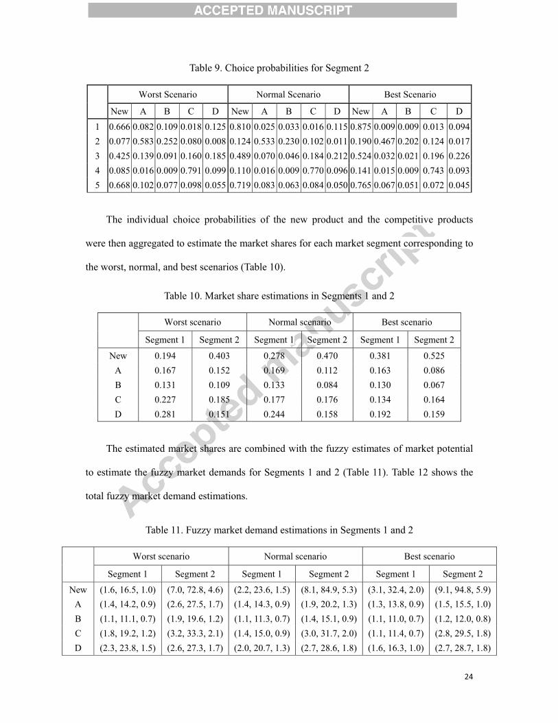
Table 9. Choice probabilities for Segment 2

Worst Scenario Normal Scenario Best Scenario

New A B C D New A B C D New A B C D 1 0.666 0.082 0.109 0.018 0.125 0.810 0.025 0.033 0.016 0.115 0.875 0.009 0.009 0.013 0.0942 0.077 0.583 0.252 0.080 0.008 0.124 0.533 0.230 0.102 0.011 0.190 0.467 0.202 0.124 0.0173 0.425 0.139 0.091 0.160 0.185 0.489 0.070 0.046 0.184 0.212 0.524 0.032 0.021 0.196 0.226 4 0.085 0.016 0.009 0.791 0.099 0.110 0.016 0.009 0.770 0.096 0.141 0.015 0.009 0.743 0.093 5 0.668 0.102 0.077 0.098 0.055 0.719 0.083 0.063 0.084 0.050 0.765 0.067 0.051 0.072 0.045

The individual choice probabilities of the new product and the competitive products

were then aggregated to estimate the market shares for each market segment corresponding to

the worst, normal, and best scenarios (Table 10).

Table 10. Market share estimations in Segments 1 and 2

Worst scenario Normal scenario Best scenario

Segment 1 Segment 2 Segment 1 Segment 2 Segment 1 Segment 2

New 0.194 0.403 0.278 0.470 0.381 0.525 A 0.167 0.152 0.169 0.112 0.163 0.086 B 0.131 0.109 0.133 0.084 0.130 0.067 C 0.227 0.185 0.177 0.176 0.134 0.164 D 0.281 0.151 0.244 0.158 0.192 0.159

The estimated market shares are combined with the fuzzy estimates of market potential

to estimate the fuzzy market demands for Segments 1 and 2 (Table 11). Table 12 shows the

total fuzzy market demand estimations.

Table 11. Fuzzy market demand estimations in Segments 1 and 2


Segment 1 Segment 2 Segment 1 Segment 2 Segment 1 Segment 2

New (1.6, 16.5, 1.0) (7.0, 72.8, 4.6) (2.2, 23.6, 1.5) (8.1, 84.9, 5.3) (3.1, 32.4, 2.0) (9.1, 94.8, 5.9) A (1.4, 14.2, 0.9) (2.6, 27.5, 1.7) (1.4, 14.3, 0.9) (1.9, 20.2, 1.3) (1.3, 13.8, 0.9) (1.5, 15.5, 1.0) B (1.1, 11.1, 0.7) (1.9, 19.6, 1.2) (1.1, 11.3, 0.7) (1.4, 15.1, 0.9) (1.1, 11.0, 0.7) (1.2, 12.0, 0.8) C (1.8, 19.2, 1.2) (3.2, 33.3, 2.1) (1.4, 15.0, 0.9) (3.0, 31.7, 2.0) (1.1, 11.4, 0.7) (2.8, 29.5, 1.8) D (2.3, 23.8, 1.5) (2.6, 27.3, 1.7) (2.0, 20.7, 1.3) (2.7, 28.6, 1.8) (1.6, 16.3, 1.0) (2.7, 28.7, 1.8)

25��

Table 12. Total fuzzy market demand estimations


New (8.6, 89.3, 5.6) (10.3, 108.5, 6.8) (12.2, 127.2, 7.9) A (4.0, 41.7, 2.6) (3.3, 34.5, 2.2) (2.8, 29.3, 1.9) B (3.0, 30.7, 1.9) (2.5, 26.4, 1.6) (2.3, 23.0, 1.5) C (5.0, 52.5, 3.3) (4.4, 46.7, 2.9) (3.9, 40.9, 2.5) D (4.9, 51.1, 3.2) (4.7, 49.3, 3.1) (4.3, 45.0, 2.8)

To estimate the crisp estimated values of the market demand of the new tablet PC, the

centroid defuzzification method was applied to calculate the crisp values for worst, normal,

and best scenarios as shown below.

<rsy � �z � � G6PE��{��P|��P� � � �z �w�Pw � ��{��}P��P| ��z � � G6PE��{��P|��P� � � �z �w�Pw � ��{��}P��P| � � GEPw�T�

<r�y � �z � � wGPJ��{��P~��Pi � � �z ��aP[ � ��{��~P|��P~ ��z � � wGPJ��{��P~��Pi � � �z ��aP[ � ��{��~P|��P~ � � �6E�T

<rxy � �z � � ��a��{��i�Pi��~ � � �z ��[aP� � ��{��|~P��i�Pi ��z � � ��aPJ��{��i�P}��~Pi � � �z ��[aP� � ��{��|~P��i�Pi � � �J?P��T

where <rsy , <r�y , and <rxy are the market demand of the new tablet PC for the worst,

normal, and best scenarios in crisp values, respectively.

To evaluate the effectiveness of the proposed model, a MNL based demand model [10,

15] as shown in Eq. (23) was employed in this research to estimate the market demands using

the same survey data sets. The model was widely used in previous studies to estimate market

demands. The estimation results based on the MNL based demand model are compared with

those based on the proposed fuzzy demand model.

26��

<ry�j� � � �� Dklmn� Dklm,o� � �� Dklm�� Dklmn

��

� ��J[�

where <ry�j� is the estimated total market demand, and �� is the market potential of the

segment i. L� is the number of respondents in the segment i. Market share of segment i is

estimated by taking average of market share estimations of L� respondents in the segment i.

With the use of the same survey data, utility functions of the MNL based demand model

were generated based on a multiple linear regression method with dummy variables. The

following shows the utility functions generated for the first respondent, �� and �i� ,

respectively for Segments 1 and 2.

�� [P�� 6Pa�� 6P�E�i � 6PG[i� � 6PG[ii � 6P[[|� � 6|i � 6PEG}� � 6~�� 6P[[~i � 6P[[h� � 6P�Ehi � JP?E�� P�E�i � 6PG[�� 6PG[�i��

�i� � ?Pa? � �P�E�� Pa�i � 6P�Ei� � 6P[[ii � 6Pa|� � 6P?E|i � 6PJJ}�� P6~� � 6P?E~i � 6h� � 6P?Ehi � 6P?E�� 6Pa�i � JP6�� P�E�i��

The utilities of the new product and four competitive products for each respondent in

Segments 1 and 2 were estimated based on the generated utility functions. Tables 13 shows

the utilities of the new product and the four competitive products of the first five respondents

in Segments 1 and 2.

Table 13. Utilities of the first five respondents in Segment 1 and Segment 2

Segment 1 Segment 2

New A B C D New A B C D 1 3.11 4.72 3.22 2.78 5.11 5.22 0.61 0.94 0.56 2.89 2 2.50 4.17 4.33 1.83 3.17 2.17 4.17 3.17 2.00 -0.67 3 4.61 3.39 2.72 4.78 4.61 3.50 1.50 1.00 2.33 2.50 4 4.56 2.78 2.44 4.06 4.06 3.50 1.17 0.50 5.83 3.33 5 4.06 3.61 2.78 4.22 4.39 5.39 2.94 2.61 2.89 2.22

27��

The choice probabilities of individuals in Segments 1 and 2 were calculated. Tables 14

shows the choice probabilities of the first five respondents in Segments 1 and 2.

Table 14. Choice probabilities of the first five respondents for Segment 1 and Segment 2

Segment 1 Segment 2

New A B C D New A B C D 1 0.066 0.329 0.073 0.047 0.485 0.885 0.009 0.012 0.008 0.086 2 0.067 0.353 0.417 0.034 0.130 0.083 0.615 0.226 0.070 0.005 3 0.276 0.081 0.042 0.326 0.276 0.527 0.071 0.043 0.164 0.194 4 0.399 0.068 0.048 0.242 0.242 0.081 0.008 0.004 0.838 0.069 5 0.222 0.143 0.062 0.263 0.310 0.785 0.068 0.049 0.064 0.033

The individual choice probabilities of the new product and the competitive products

were then aggregated to estimate the market shares of each market segment (Table 15).

Table 15. Market share estimations in Segments 1 and 2

Segment 1 Segment 2

New 0.274 0.499 A 0.187 0.108 B 0.133 0.079 C 0.172 0.165 D 0.234 0.148

Figure 6 compares the market share of the new product estimated based on the proposed

model and MNL based model.

28��

.

Figure 6. Comparison of the market share estimation of the new product.

The market potential �� can be estimated by taking average of those estimated by

marketing executives. For this case, the market potentials of Segment 1 and 2 were calculated

as 84.9 K and 180.5 K, respectively. Thus, the market demand of the new product is

estimated as 113.3 K based on the MNL based demand model. It can be noted that the

estimated market demand based on the MNL based model is very close to that for the normal

scenario based on the proposed model which is 107 K. However, the MNL based demand

model cannot provide market demand estimations for other scenarios that companies may

need to consider in the risk assessment of NPD projects while the proposed model can

provide the estimated market demands for both the worst, and best scenarios. Figure 7

compares the total market demands of the new product estimated based on the proposed

model and MNL based model.

0

0.1

0.2

0.3

0.4

0.5

0.6

Segment�1 Segment�2

A�� Worst�Scenario�(proposed�model)

B�� Normal�Scenario�(proposed�model)

C�� Best�Scenario�(proposed�model)

D�� MNL�based

A

B

C

D

A

BC

D

29��

Figure 7. Comparison of the total market demands of the new product.

The prices of tablet PCs which has similar specifications as the new tablet PC proposed

by the NPD team in this case are around USD 513. Since the green index of the proposed

new tablet PC is 3, the price of the new tablet PC could be set as about USD 385. If the profit

margin without considering the expenses of R&D, product development and marketing is

25%, the profit per tablet PC is about USD 96. Therefore, the total profits are around USD

8.4M, 10.3M, and 12.1M for the worst, normal, and best scenarios, respectively. However, it

is common for a company to invest millions of US dollars on R&D, product development and

marketing regarding development and marketing of a new tablet PC. Thus, the senior

management of the company may think that the profit generated from the NPD project in the

worst scenario may not be good enough for the company to take the risk of conducting the

NPD project even though it may seem to be quite profitable in the normal scenario. Hence,

the proposed fuzzy demand model can provide more information to decision makers in

assessing financial viability of NPD projects.�

4. Conclusion and Further Study

Market demand estimation involves various uncertainties such as inconsistent customer

A� �

B �

C � �D �

0

20

40

60

80

100

120

140

The Total Market Demand ( K)

A - Worst Scenario (proposed model)B - Normal Scenario (proposed model)C - Best Scenario (proposed model)D - MNL-based

30��

behavior, subjective responses of respondents in surveys, unstable market conditions, and

technological development. Two uncertainties are addressed in this research. One is the

subjective judgment of respondents on product profiles in conjoint surveys, which can lead to

a high degree of fuzziness of survey data. Another is the group estimation of market potential

based on a jury of executive opinion method. The two uncertainties have not been considered

in previous studies regarding the development of market demand models. In this paper, a

novel methodology is proposed for market demand estimation while addressing the two

uncertainties. In the proposed methodology, fuzzy regression is introduced into DCA to

address the fuzziness of survey data and fuzzy estimates are generated to address the

fuzziness of the market potential estimation. The developed fuzzy market demand models can

help decision makers examine market demands under different scenarios. The estimated

market demands can also be used to estimate the profits of a NPD project under the worst,

normal, and best scenarios. Those estimated profits under different scenarios are useful for

companies to assess the financial viability of NPD projects. A case study of market demand

estimation of a new tablet PC was conducted based on the proposed methodology to illustrate

the applicability and evaluate the effectiveness of the methodology. The results of the case

study are compared with those based on a popular MNL based demand model. From the

comparison, it can be noted that the estimated market demand based on the MNL model is

very close to that for the normal scenario based on the proposed fuzzy demand model.

However, the MNL model cannot provide estimates for different scenarios while the

proposed model can provide estimated market demands for both the worst, and best scenarios.

In this research, the proposed methodology was applied on market demand estimation of

tablet PCs. In fact, the methodology can be applied on any type of products so long as the

products do not monopolize their markets.

To improve the modeling accuracy of the fuzzy utility functions, the fuzzy least square

31��

regression method can be used to generate the functions, specifically when survey data

contains random errors. In this paper, prices of the new and competing products are not

considered but they may have significant effects on market demand estimation. Future work

could consider the prices in the demand estimation. On the other hand, in this research, only

triangular member functions were adopted. Thus, future work could involve a study of the

effects of different membership functions on the results of demand estimation. This study can

also be extended to consider dynamic consumer preferences and develop a time-varying

market share model. Markov Chain steady state analysis can be introduced to address the

dynamic issue.

Acknowledgement

This work was supported by Hong Kong Polytechnic University (A/C No. RTQ9).

References�

[1] W. Chen, C. Hoyle, H.J. Wassenaar, Decision-Based Design: Integrating Consumer

Preferences into Engineering Design, Springer-Verlag, London, 2013.

[2] D.J. Dalrymple, Sales forecasting practices: Results from a United States survey, Int. J. of

Forecasting. 3 (1987) 379-391.

[3] P. Diamond, H. Tanaka, Fuzzy regression analysis, in: R. Slowinski (Ed.), Fuzzy Sets in

Decision Analysis, Operations Research and Statistics, Kluwer Academic Publishers, Boston,

1998, pp. 349-387.

[4] C. Hoyle, W. Chen, N. Wang, F.S. Koppelman, Integrated Bayesian hierarchical choice

modeling to capture heterogeneous consumer preferences in engineering design, J. of

Mechanical Design (ASME). 132 (2010).

[5] C. Kahraman, A. Beskese, F.T. Bozbura, Fuzzy regression approaches and applications, in:

C. Kahraman (Ed.), Fuzzy Applications in Industrial Engineering, Springer-Verlag, Berlin,

Heidelberg, New York, 2006, pp. 589-615.

32��

[6] R.B. Kazemzadeh, M. Behzadian, M. Aghdasi, A. Albadvi, Integration of marketing

research techniques into house of quality and product family design, Int. J. Adv.

Manufacturing Technology. 41 (2009) 1019-1033.

[7] B. Kosko, Fuzziness vs. probability, Int. J. General Systems. 17 (1990) 211-240.

[8] D. Kumar, W. Chen, T.W. Simpson, A market-driven approach to product family design,

Int. J. of Production Research. 47 (2009) 71-104.

[9] M. Kuzmanovic, M. Martic, An approach to competitive product line design using

conjoint data, Experts Systems with Applications. 39 (8) (2012) 7262-7269.

[10] C.K. Kwong, X.G. Luo, J.F. Tang, A multiobjective optimization approach for product

line design, IEEE Transactions on Engineering Management. 58 (1) (2010) 97-108.

[11] K. Lau, A. Kagan, G.V. Post, Market share modeling within a switching regression

framework, Omega, The Int. Journal of Management Science. 25 (3) (1997) 345-353.

[12] W.V. Leekwijck, E.E. Kerre, Defuzzification: criteria and classification, Fuzzy Sets and

Systems. 108 (1999) 159-178.

[13] A. Lemos, D. Leite, L. Maciel, R. Ballini, W. Caminhas, F. Gomide, Evolving fuzzy

linear regression tree approach for forecasting sales volume of petroleum products, in: IEEE

World Congress on Computational Intelligence (WCCI), 2012.

[14] K.H. Lin, L.H. Shih, Y.T. Cheng, S.C. Lee, Fuzzy product line design model while

considering preferences uncertainty: A case study of notebook computer industry in Taiwan,

Expert Systems with Applications. 38 (2011) 1789-1797.

[15] K.H. Lin, L.H. Shih, S.C. Lee, Optimization of product line design for environmentally

conscious technologies in notebook industry, Int. J. Environ. Sci. Tech. 7 (3) (2010) 473-484

[16] J.J. Louviere, D.A. Hensher, J.D. Swait, Stated Choice Methods: Analysis and

Application. Cambridge University Press, Cambridge, 2000.

[17] D. McFadden, The measurement of urban travel demand, J. of Publics Economics 3.

(1974) 303-328.

[18] T. Mori, Taguchi methods, ASME Press, New York, 2011.

33��

[19] G. Peters, Fuzzy linear regression with fuzzy intervals, Fuzzy Sets and Systems. 63

(1994) 45-55.

[20] S.S. Razu, S. Takai, Reliability and accuracy of bootstrap and Monte Carlo methods for

demand distribution modeling, in: proceedings of the 5th Annual ISC Research Symposium,

2011.

[21] C.B. Resende, C.G. Heckmann, J.J. Michalek, Robust design for profit maximization

under uncertainty of consumer choice model parameters using the delta method, in:

proceedings of the ASME Design Engineering Technical Conferences and Computers in

Engineering Conference, 2011.

[22] A.F. Shapiro, Fuzzy regression models, ARC (Actuarial Research Conference), 2005.

[23] H. Tanaka, H. Ishibuchi, Possibilistic regression analysis based on linear programming,

in: J. Kacprzyk, M. Fedrizzi (Eds.), Fuzzy Regression Analysis, Omnitech Press, Warsaw and

Physica-Verlag, Heidelberg, 1992, pp. 47-60.

[24] H. Tanaka, Fuzzy data analysis by possibilistic linear model, Fuzzy Sets and Systems. 24

(1987) 363-375.

[25] H. Tanaka, S. Uegima, K. Asai, Linear regression analysis with fuzzy model, IEEE

Transactions on Systems, Man, and Cybernetics. 12 (1982) 903-907.

[26] K.E. Train, Discrete Choice Methods with Simulation, Cambridge University Press,

Cambridge, 2009.

[27] I.B. Turksen, I.A. Willson, A fuzzy set preference model for consumer choice, Fuzzy

Sets and Systems. 68 (1994) 253-266.

[28] N.A. Williams, S. Azarm, P.K. Kannan, Multicategory design of bundled products for

retail channels under uncertainty and competition, J. of Mechanical Design (ASME). Vol. 132

(2010).

[29] Y. Xiong, G. Li, K.J. Fernandes, Dynamic pricing model and algorithm for perishable

products with fuzzy demand. Applied Stochastic Models in Business and Industry. 26 (2010)

758-774.

34��

R. Aydin received B.Eng. degrees in Industrial Engineering and Energy Systems Engineering

from Bahcesehir University, Istanbul, Turkey, in 2011 and 2012, respectively. He is currently

working towards a Ph.D. degree in the Department of Industrial and Systems Engineering of

The Hong Kong Polytechnic University, Hong Kong. His research interests include new

product development and green supply chain management.

Dr. C.K. Kwong received the M.Sc. degree in Advanced Manufacturing System from the

University of Nottingham, U.K., and the Ph.D. degree in Manufacturing Engineering from

the University of Warwick, Warwick, U.K. Dr. Kwong currently is an Associate Professor in

the Department of Industrial and Systems Engineering of The Hong Kong Polytechnic

University, Hong Kong. His research interests include new product development, product line

design, design for manufacture, and integrated design.

Dr. P. Ji received the BSc degree from Northeastern Heavy Machinery Institute and a MSc

degree from Beihang University, PRC. He started his academic career since 1984 when he

joined Beihang University as an assistant lecturer. After received his PhD degree from West

Virginia University, USA in 1992, he joined National University of Singapore. He then joined

The Hong Kong Polytechnic University in 1996. Currently Dr. Ji is an Associate Professor in

the Department of Industrial and Systems Engineering of The Hong Kong Polytechnic

University. His research areas are operation management and optimization.

Dr. H.C.M. Law received the BEng(Hons) degree in Manufacturing Engineering and a

MPhil degree and a PhD degree in Environmental Engineering all from The Hong Kong

Polytechnic University, Hong Kong. He currently is a product research and development

manager of G.E.W International Corporation Limited, Hong Kong. His research interests

are new product development and environmental engineering.

Ridvan A

Dr. C.K.

Dr. P. Ji

Dr. H.C.

Aydin

Kwong

M. Law

market demand estimation for new product development by using fuzzy modeling and discrete choice...

Documents