edited by

DAVID BURCH

www.starpathpublications.com

MARINER’S PRESSURE ATLAS

Worldwide Mean Sea Level Pressures and Standard Deviations

for Weather Analysis and Tropical Storm Forecasting

Copyright © 2014 Starpath Publications

All rights reserved. No part of this book may be reproduced or transmitted in any form or by any means, electronic or mechanical, including photocopying, record-ing, or any information storage or retrieval system, without permission in writing from the publisher.

ISBN 978-0-914025-38-2

Published by

Starpath Publications

3050 NW 63rd Street, Seattle, WA 98107

www.starpathpublications.com

“The slightest deviation from the barometric mean between the tropics demands on the part of the commander immediate attention.”

— The Mercantile Marine Magazine, Vol 1, January, 1854, page 8.

At the time of that quote, mariners were using mercury barometers. Three months later in the April issue, they brought up this point again in an article that compares the then new aneroid barometers with the traditional mercury barometers. They speculated that the aneroids may not be linear over their full range and called for a careful study before the above pressure observations will be useful.

This is exactly what happened. Traditional mercury barometers were very tedious to use at sea, but they were accurate once known corrections were made. Common aneroids at the time were not accurate over full range, and before the Internet came about it was very difficult to calibrate an aneroid device. So the use of accurate pressure observations fell out of modern teaching (as the aner-oids replaced mercury devices)—nevertheless, the proposal has been mentioned in Bowditch throughout the years. Now with good electronic barometers and convenient ways to calibrate any barometer, we can again use this valuable in-formation for tropical storm warnings.

Contents

Introduction ....................................................................................................................................... 1

The Data .............................................................................................................................................. 2

Data Comparisons ............................................................................................................................. 4

Tropical Storms .................................................................................................................................. 5

Barometric Pressure in the Tropics ................................................................................................. 6

Bowditch on Pressure in the Tropics ............................................................................................... 8

Worldwide Mean Sea Level Pressures and Standard Deviations ................................................ 9

January — Mean Sea Level Pressure (mb) ......................................................................... 10

January — Standard Deviations (mb) ................................................................................ 12

February — Mean Sea Level Pressure (mb) ...................................................................... 14

February — Standard Deviations (mb) .............................................................................. 16

March — Mean Sea Level Pressure (mb) ........................................................................... 18

March — Standard Deviations (mb) .................................................................................. 20

April — Mean Sea Level Pressure (mb) ............................................................................. 22

April — Standard Deviations (mb) ..................................................................................... 24

May — Mean Sea Level Pressure (mb) ............................................................................... 26

May — Standard Deviations (mb) ...................................................................................... 28

June — Mean Sea Level Pressure (mb) .............................................................................. 30

June — Standard Deviations (mb) ...................................................................................... 32

July — Mean Sea Level Pressure (mb) ................................................................................ 34

July — Standard Deviations (mb) ....................................................................................... 36

August — Mean Sea Level Pressure (mb) .......................................................................... 38

August — Standard Deviations (mb) ................................................................................. 40

September — Mean Sea Level Pressure (mb) .................................................................... 42

September — Standard Deviations (mb) ........................................................................... 44

October — Mean Sea Level Pressure (mb) ........................................................................ 46

October — Standard Deviations (mb) ............................................................................... 48

November — Mean Sea Level Pressure (mb) .................................................................... 50

November — Standard Deviations (mb) ........................................................................... 52

December — Mean Sea Level Pressure (mb) .................................................................... 54

December — Standard Deviations (mb) ........................................................................... 56

1

Introduction

The primary goal of this publication is to make mariners more aware of barometric pressure and how it might add to the safety and efficiency of their time on the water and to provide a specific, dependable method of storm warning in the tropics.

It is also intended to show the great value of an accurate barometer. The days of only caring about rise and fall, fast or slow, should be relegated to the history books. We now have ready access to accurate instruments and all the benefits they provide.

In the past barometric pressure was taught to mariners only on a relative scale–is the pressure rising or falling, and how fast. Almost never was the role of the actual value of the pressure incorporated into the teaching. The primary reason for that was probably because many mariners did not concern themselves with the calibration of their barometers, and that because there was no easy way to do so.

Without dependable pressure readings, one learns very quickly that the actual reading on the dial is not a useful number. Several vessels moored nearby might have large differences in their pressure readings.

That has changed now. With the advent of accurate barometers, both electronic and aneroid, and easy ways to monitor their calibration with Internet reports of accurate pressure, all mariners can now have a barometer on board that will read the correct atmospheric pressure, not to mention that they can now observe the rise and fall at the proper rates. It was known in the 1800s that aneroid barometers were often not linear, which meant that even their indicated rate of change could be far from the truth.

It should be added immediately that there always have been a handful of truly dependable aneroid barometers on the market, but these were and remain expensive instruments. New developments in electronic barometers gives us promise that we can achieve this same or improved accuracy at much more economical costs.

Barometer awareness starts with knowing what typical pressures are and how they vary with the season and location, and that is precisely the content of this publication.

This knowledge for mariners is even more important today than it was in the early days of sailing when it was first being learned. Ironically, the more convenient the weather forecasts become, the more we are dependent on our own observations to check them.

Many if not most mariners underway rely heavily on numerical weather prediction passed on to them at sea via GRIB format. These model forecasts give precise wind and pressure values up to 7 days out, but other than the very first of the map sequence, these are unvetted numerical predictions from just one of the several models used in the official forecasts. Our own observations of wind speed and direction and especially the barometric pressure and its tendency are required to evaluate the GRIB data, and even the official forecasts. The overall pressure patterns and related winds are remarkably good, but the timing of them and their precise location can only be confirmed by our own observations.

Thus measuring an accurate pressure at the synoptic times to compare with the weather maps becomes a standard procedure in modern marine weather analysis.

Another value of this global record of pressures in modern times is the frequency that mariners travel to new parts of the world to begin their voyage. The data shows that the barometer behaves quite differently in different parts of the world.

Those accustomed to weather work in Boston or Seattle, for example, might observe a January pressure of 1017 mb, and then the next day or so note it has dropped to 1011 mb, and unless it had really plummeted down, they would not be particularly alarmed. They have seen this many times with no severe change in weather. The average pressure in January in these regions is about 1017 mb, but with a January standard deviation of 10 or so mb, this observed pressure drop is not out of the ordinary.

The same pressure drop of 6 mb for those living in the tropics in hurricane season, on the other hand, would be a huge and imminent warning for a tropical storm. The main difference is the expected variations in pressure (standard deviations) and that is the primary data of this book.

With the monthly average pressures and the standard deviations, an accurate barometer in the tropics provides a way to forecast an approaching tropical storm or hurricane that can be very useful if you are left without radio or satellite phone communications. Even with forecasts in hand, this technique offers valuable confirmation on the timing of an approaching system.

Outside of the tropics, this data has more indirect value. It shows the source and pattern of monthly climatic wind patterns worldwide, as well as offering a perspective on the magnitudes of barometric pressures more generally. In practice there is no official definition of high or low pressure, it is always relative. But since we include the standard deviations of the pressure from the average value, we do indeed have a way to evaluate the pressures we observe relative to the expected variation. It is not as good a forecasting tool outside of the tropics when the standard deviations are large, but the statistical meanings of these deviations remain the same.

For more details on marine weather and barometer use and calibration in particular we recommend two other books from Starpath Publications: Modern Marine Weather and The Ba-rometer Handbook.

2

The DataThe atmospheric pressure statistics presented here are reproduced from the U.S. Navy Marine Climatic Atlas of the World, Vol IX, 1981. The original data set was assembled in the late 1950s and early 1960s from many nations covering over 120 years, largely from ship observations recorded in logbooks. Thus we only have full data over the oceans of the world.

They were then averaged over 5° quadrangles, and smooth lines drawn through these average values. These data were originally distributed as a DOS computer program on floppy disks, with a few rare printed editions.

Potential errors come about because all data are included in the monthly averages, whereas there is no distinction between time of day or time of month. If a particular station had mostly data from early in the day, or only from the end of the month, then that data could be biased. The original text states that there is no indication that this biases the results. According to the Navy Atlas, the “operationally significant accuracy” of the data is considered to be ±1 mb. This accuracy estimate refers to the marine data over the water. The NWS provided average isobars for the land, but the blending together of the data sets is not always uniform. There are no standard deviations for the land data.

Another question might be related to the age of the data, now quite old. Comparable temperature data could in principle reflect some element of global warming, but there does not seem to be any notable trend in this pressure data. We have tested this several ways, notably using archived data from the National Climatic Data Center. Samples comparisons are given in the next section

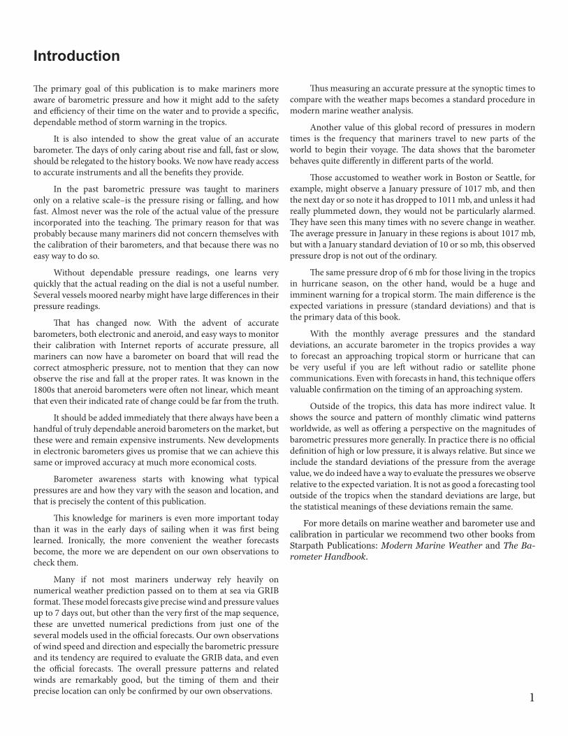
The pressures presented are the mean sea level pressure averaged over the month. It is defined in the usual way as the sum of all values divided by the number of values. Also presented here are the standard deviations of the data for each month. The standard deviation (SD) of a set of data is a measure of its variability. It is the average difference of all values from the mean value. When the SD is small, the data are clustered closely around the mean value, when the SD is large, there is much more variation in the values, as illustrated in Figure 1.

The SD can be used to understand pressure probabilities because studies show that an extended set of pressure measurements for the same location follows what mathematicians call the normal distribution (bell curve). This curve describes much of what we see in nature that stems from more or less random distinctions. The heights of American women, for example, between ages of 18 and 24 follows a normal distribution with a mean value of 65.5 inches and a standard deviation (SD) of 2.5 inches. This SD determines the spread in heights we might encounter.

In normal distributions it is easy to predict the probability of values that differ from the mean value of the data set, as shown in Figure 1. From this distribution we can make Table 1 that tells us about the pressures we might observe and what they can mean.

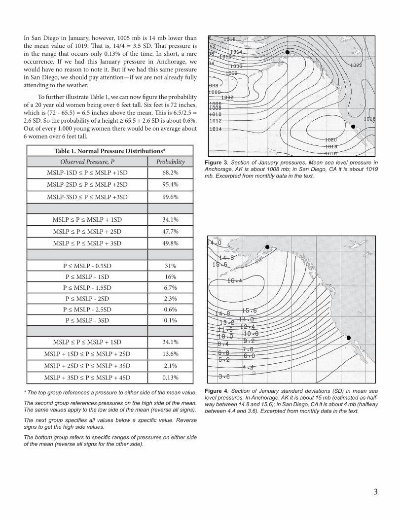
As an example, refer to the sample January data in Figures 3 and 4 for Anchorage, AK and San Diego, CA. In each case some interpolation is called for to learn that the January MSLP in Anchorage is 1008 mb with an SD of 15 mb, and in San Diego it is 1019 mb with an SD of about 4 mb. Evaluating the Anchorage statistics with Table 1, we see that in Anchorage 68% of all January pressures will be between 993 mb and 1023 mb (1008 ±15). Any pressure outside of that range has only a 32% chance of occurring (100% - 68%).

A pressure of 1005 mb, for example, in January in Anchorage is fairly common. It is in the range that occurs 34% of the time.

Figure 1. Three normal distributions of (say) 100 measurements with 3 different standard deviations (SD). When SD is small, the values are all near the mean value (like monthly pressures in the tropics); when it is large they are more spread out (like pressures at high latitudes). To find the SD of a set of numbers, first find the average, then make a list of all the differences between each value and the average, then square each difference (to cancel what side of the average it is on), then find the average of these squared differences, and then take the square root of that. In this sense, the SD is the average difference from the mean for the full set.

SD = 0.4

SD = 1.0

SD = 2.2

1.00.9

0.80.7

0.6

0.5

0.40.3

0.2

0.1

00 1 2 3 4 5-5 -4 -3 -2 -1

Rela

tive

Num

ber o

f Obs

erva

tions

Di�erence from Mean Value

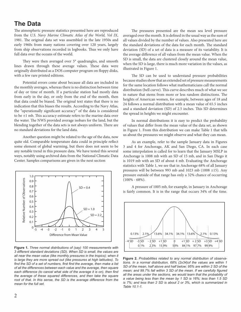
Figure 2. Probabilities related to any normal distribution of observa-tions. In a normal distribution, 68% (2x34)of the values are within 1 SD of the mean, half above and half below; 95% are within 2 SD of the mean; and 99.7% fall within 3 SD of the mean. If we carefully figured all the areas under the sections, we would learn that the probability of a value being less than the mean by 1 SD is 16%; less than 1.5 SD is 7%; and less than 2 SD is about 2 or 3%, which is summarized in Table 10.1-1.

0.13% 2.1% 13.6% 34.1% 34.1% 13.6% 2.1% 0.13%

0 +1 SD + 2 SD +3 SD +4 SD- 4 SD -3 SD - 2 SD +1 SD50% 84.1% 97.7% 99.9%0.1% 2.3% 15.9%

3

In San Diego in January, however, 1005 mb is 14 mb lower than the mean value of 1019. That is, 14/4 = 3.5 SD. That pressure is in the range that occurs only 0.13% of the time. In short, a rare occurrence. If we had this January pressure in Anchorage, we would have no reason to note it. But if we had this same pressure in San Diego, we should pay attention—if we are not already fully attending to the weather.

To further illustrate Table 1, we can now figure the probability of a 20 year old women being over 6 feet tall. Six feet is 72 inches, which is (72 - 65.5) = 6.5 inches above the mean. This is 6.5/2.5 = 2.6 SD. So the probability of a height ≥ 65.5 + 2.6 SD is about 0.6%. Out of every 1,000 young women there would be on average about 6 women over 6 feet tall.

Table 1. Normal Pressure Distributions*Observed Pressure, P Probability

MSLP-1SD ≤ P ≤ MSLP +1SD 68.2%

MSLP-2SD ≤ P ≤ MSLP +2SD 95.4%

MSLP-3SD ≤ P ≤ MSLP +3SD 99.6%

MSLP ≤ P ≤ MSLP + 1SD 34.1%

MSLP ≤ P ≤ MSLP + 2SD 47.7%

MSLP ≤ P ≤ MSLP + 3SD 49.8%

P ≤ MSLP - 0.5SD 31%

P ≤ MSLP - 1SD 16%

P ≤ MSLP - 1.5SD 6.7%

P ≤ MSLP - 2SD 2.3%

P ≤ MSLP - 2.5SD 0.6%

P ≤ MSLP - 3SD 0.1%

MSLP ≤ P ≤ MSLP + 1SD 34.1%

MSLP + 1SD ≤ P ≤ MSLP + 2SD 13.6%

MSLP + 2SD ≤ P ≤ MSLP + 3SD 2.1%

MSLP + 3SD ≤ P ≤ MSLP + 4SD 0.13%

* The top group references a pressure to either side of the mean value.

The second group references pressures on the high side of the mean. The same values apply to the low side of the mean (reverse all signs).

The next group specifies all values below a specific value. Reverse signs to get the high side values.

The bottom group refers to specific ranges of pressures on either side of the mean (reverse all signs for the other side).

Figure 3. Section of January pressures. Mean sea level pressure in Anchorage, AK is about 1008 mb; in San Diego, CA it is about 1019 mb. Excerpted from monthly data in the text.

Figure 4. Section of January standard deviations (SD) in mean sea level pressures. In Anchorage, AK it is about 15 mb (estimated as half-way between 14.8 and 15.6); in San Diego, CA it is about 4 mb (halfway between 4.4 and 3.6). Excerpted from monthly data in the text.

4

Data ComparisonsAs noted earlier we have compared this data from the U.S. Navy Marine Climatic Atlas of the World (MCAW) with more modern data from the National Climatic Data Center (NCDC). A sample comparison is shown in Table 2. It is representative of the comparisons we made this way at several US coastal locations.

Figure 5 shows a comparison of the Navy Data (MCAW) with the latest US Pilot Chart data, but frankly much of the latter is as old as the Navy data. What is unique in the Navy data presented in this book are the standard deviations, which are crucial to understanding and interpreting pressure changes.

* MCAW is the US Navy Marine Climatic Atlas of the World. NCDC isthe National Climatic Data Center. The former data are presented inthis book; the latter are available from the NCDC. The agreement isgenerally very good, since the values of the SD are the most crucial. Inseveral midlatitude coastal comparisons we found the SD are within ±1mb, even when the MSLP might be off several mb.

Table 2. Nantucket Island Pressures*

MCAW <1980 NCDC 1988-2008

Month MSLP SD MSLP SD

Jan 1016.4 10.0 1016.7 9.9

Feb 1015.2 10.8 1014.7 9.5

Mar 1014.7 10.0 1014.7 10.2

Apr 1015.5 9.0 1012.8 8.6

May 1016.0 6.9 1014.7 7.1

Jun 1015.0 6.1 1014.3 6.6

Jul 1016.0 5.2 1014.3 5.1

Aug 1016.0 5.1 1015.5 4.9

Sep 1017.0 6.8 1016.3 6.8

Oct 1017.5 8.0 1016.3 8.6

Nov 1016.0 9.2 1016.7 9.4

Dec 1016.0 9.4 1015.9 10.3

October Pilot Chart

October MSLP

October SD

Figure 5. Right. MSLP pressure data from a US Pilot Chart compared to the MCAW data. The pressures agree well, but there is no compa-rable data for the important standard deviations. The Pilot Charts are online, so this type of comparison can be made for any month and any part of the world. The other lines on the Pilot charts are average tem-peratures (ºC) and the faint lines are the magnetic variations.

7

121

2

3

4

56

7

8

9

10

11

FALLING

RISING

AVG

AVG

MIN

MAX

TROPICAL BARO CLOCK

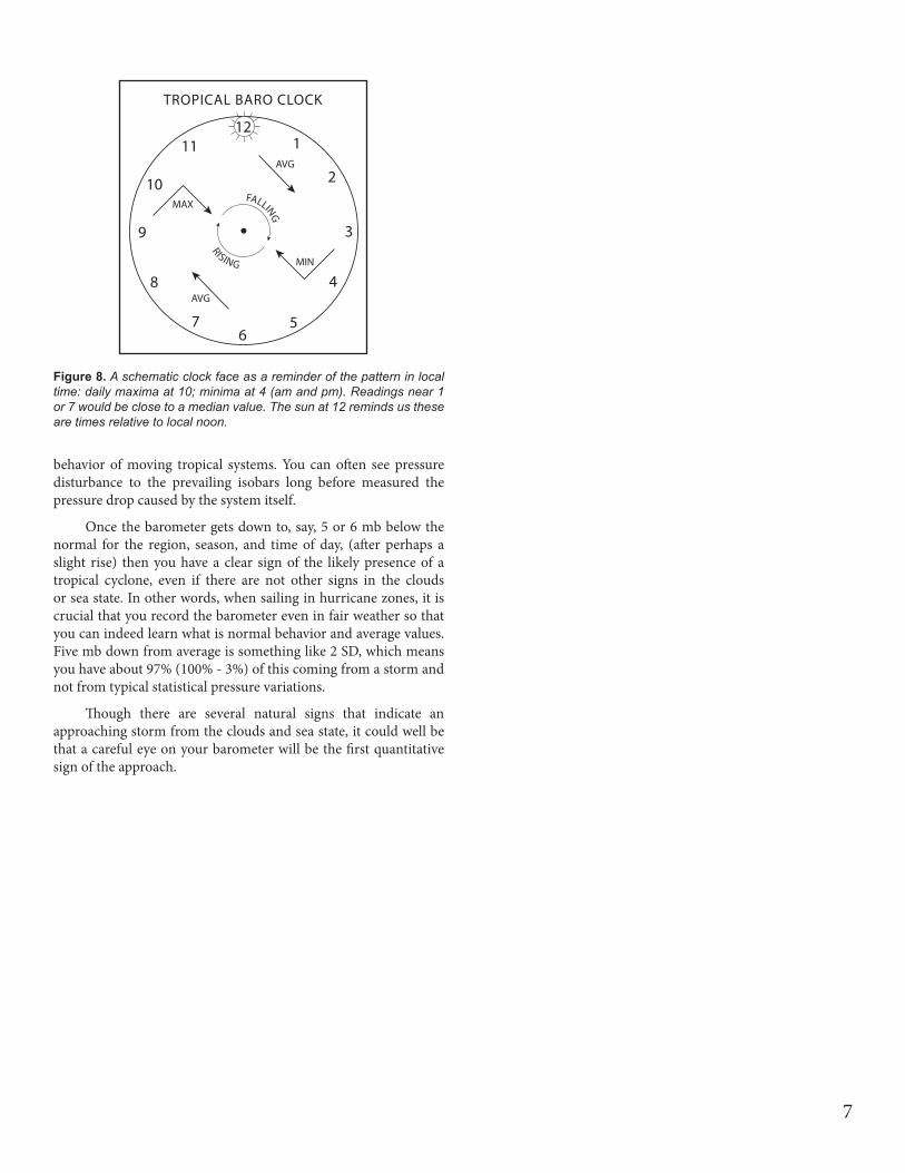
Figure 8. A schematic clock face as a reminder of the pattern in local time: daily maxima at 10; minima at 4 (am and pm). Readings near 1 or 7 would be close to a median value. The sun at 12 reminds us these are times relative to local noon.

behavior of moving tropical systems. You can often see pressure disturbance to the prevailing isobars long before measured the pressure drop caused by the system itself.

Once the barometer gets down to, say, 5 or 6 mb below the normal for the region, season, and time of day, (after perhaps a slight rise) then you have a clear sign of the likely presence of a tropical cyclone, even if there are not other signs in the clouds or sea state. In other words, when sailing in hurricane zones, it is crucial that you record the barometer even in fair weather so that you can indeed learn what is normal behavior and average values. Five mb down from average is something like 2 SD, which means you have about 97% (100% - 3%) of this coming from a storm and not from typical statistical pressure variations.

Though there are several natural signs that indicate an approaching storm from the clouds and sea state, it could well be that a careful eye on your barometer will be the first quantitative sign of the approach.

8

Bowditch on Pressure in the Tropics

The American Practical Navigator, Pub. 9, originally by Nathaniel Bowditch, nicknamed “Bowditch,” is a primary reference on marine navigation and weather. Bowditch includes an extensive and valuable chapter on Tropical Storms. The section on statistical analysis is reproduced below, but the required data has not been readily available for the past 20 years or so.

3510. Statistical Analysis of Barometric Pressure. A method for alerting the mariner to possible tropical cyclone formation involves a statistical comparison of observed weather parameters with the climatology (30 year averaged conditions) for those parameters. Significant fluctuations away from these average conditions could mean the onset of severe weather.

One such statistical method involves a comparison of mean surface pressure in the tropics with the standard deviation (s.d.) of surface pressure. Any significant deviation from the norm could indicate proximity to a tropical cyclone. Analysis shows that surface pressure can be expected to be lower than the mean minus 1 s.d. less than 16% of the time, lower than the mean minus 1.5 s.d.

less than 7% of the time, and lower than the mean minus 2 s.d. less than 3% of the time. Comparison of the observed pressure with the mean will indicate how unusual the present conditions are.

As an example, assume the mean surface pressure in the South China Sea to be about 1005 mb during August with a s.d. of about 2 mb. Therefore, surface pressure can be expected to fall below 1003 mb about 16% of the time and below 1000 mb about 7% of the time. Ambient pressure any lower than that would alert the mariner to the possible onset of heavy weather. Charts showing the mean surface pressure and the s.d. of surface pressure for various global regions can be found in the U.S. Navy Marine Climatic Atlas of the World. [Editors’ note: these are the data included in this book—and there is an unstated important assumption is that the mariner has an accurate barometer to make the observations.]

10

January — Mean Sea Level Pressure (mb)

13