marine distributions of chinook salmon from the west coast
TRANSCRIPT

This article was downloaded by: [Oregon State University]On: 17 August 2011, At: 16:29Publisher: Taylor & FrancisInforma Ltd Registered in England and Wales Registered Number: 1072954 Registeredoffice: Mortimer House, 37-41 Mortimer Street, London W1T 3JH, UK
Transactions of the American FisheriesSocietyPublication details, including instructions for authors andsubscription information:http://www.tandfonline.com/loi/utaf20
Marine Distributions of ChinookSalmon from the West Coast of NorthAmerica Determined by Coded Wire TagRecoveriesLaurie A. Weitkamp aa National Marine Fisheries Service, Northwest Fisheries ScienceCenter, Newport Field Station, 2032 Southeast Oregon StateUniversity Drive, Newport, Oregon, 97365, USA
Available online: 09 Jan 2011
To cite this article: Laurie A. Weitkamp (2010): Marine Distributions of Chinook Salmon fromthe West Coast of North America Determined by Coded Wire Tag Recoveries, Transactions of theAmerican Fisheries Society, 139:1, 147-170
To link to this article: http://dx.doi.org/10.1577/T08-225.1
PLEASE SCROLL DOWN FOR ARTICLE
Full terms and conditions of use: http://www.tandfonline.com/page/terms-and-conditions
This article may be used for research, teaching and private study purposes. Anysubstantial or systematic reproduction, re-distribution, re-selling, loan, sub-licensing,systematic supply or distribution in any form to anyone is expressly forbidden.
The publisher does not give any warranty express or implied or make any representationthat the contents will be complete or accurate or up to date. The accuracy of anyinstructions, formulae and drug doses should be independently verified with primarysources. The publisher shall not be liable for any loss, actions, claims, proceedings,demand or costs or damages whatsoever or howsoever caused arising directly orindirectly in connection with or arising out of the use of this material.

Marine Distributions of Chinook Salmon from the West Coast ofNorth America Determined by Coded Wire Tag Recoveries
LAURIE A. WEITKAMP*National Marine Fisheries Service, Northwest Fisheries Science Center, Newport Field Station,
2032 Southeast Oregon State University Drive, Newport, Oregon 97365, USA
Abstract.—The coded wire tag (CWT) database contains detailed information on millions of Pacific salmon
Oncorhynchus spp. released from hatcheries or smolt traps and recovered in the north Pacific Ocean and its
tributaries. I used this data set to examine the spatial and temporal variation in the marine distributions of 77
hatchery and 16 wild populations of Chinook salmon O. tshawytscha based on recoveries of an estimated
632,000 tagged salmon in coastal waters from southern California to the Bering Sea during 1979–1994 (and
1995–2004 for select hatcheries). Chinook salmon showed 12 distinct region-specific recovery patterns.
Chinook salmon originating in a common freshwater region had similar marine distributions, which were
distinct from those of adjacent regions. Different run types (e.g., spring, summer, and fall runs) originating in
the same region exhibited variation in their marine distributions consistent with recovery at different stages of
their ocean residence period. Recovery patterns were surprisingly stable across years, despite high interannual
variation in ocean conditions. By contrast, ocean age influenced recovery patterns, as older fish were
recovered further from their natal stream than younger fish. Although most of the CWT data used in the
analysis came from hatchery fish, recoveries of tagged wild populations indicate patterns similar to those of
fish from nearby hatcheries. The consistency in these findings across broad geographic areas suggests that
they apply to Chinook salmon across the entire Pacific Rim. Similar findings for tagged coho salmon O.
kisutch indicate that the observed patterns may apply to Pacific salmon as a whole and provide a model for
other highly migratory fishes that have not benefited from such intensive tagging programs. The results also
have implications for the genetic control of migration and salmon’s ability to respond to climate change.
Knowing the spatial dynamics of an organism—
where it is located during each stage of its life—is
crucial to understanding the factors affecting its
survival and reproductive success (Leggett 1985). This
is particularly true for anadromous Pacific salmon
Oncorhynchus spp. because of their use of both
freshwater and marine environments. Although Pacific
salmon spend most of their life in marine waters,
relatively little is know about their location during
marine residence or the factors affecting their distribu-
tion or survival (Pearcy 1992; Quinn 2005). Better
knowledge of these factors is critical for effective
management but is also necessary to understand the
basic biology and, therefore, long-term survival of
these culturally and commercially important species.
Chinook salmon O. tshawytscha have long been the
focus of tagging studies used to determine oceanic
distributions and origins of particular stocks (Neave
1964; Major et al. 1978). Early work determined that
salmon from different freshwater regions had different
marine distributions, although there was considerable
spatial and temporal overlap in distributions (Milne
1957; Wright 1968). Studies in large river basins such
as the Columbia River determined that Chinook
salmon from different parts of the basin or with
different run types also had different marine distribu-
tions (Wahle and Vreeland 1978; Wahle et al. 1981).
(Chinook salmon display variation in the timing when
returning adults enter rivers to spawn [termed ‘‘run
type’’]. These run types typically consist of spring,
summer, or fall runs, based on when they reenter
freshwater.) Using ocean distribution information for
Chinook salmon from North America, Healey (1983)
suggested that stream-type Chinook salmon (those with
yearling smolts, typically spring and some summer run
populations) have a much more offshore distribution
than do ocean-type Chinook salmon (those with
subyearling smolts, typically fall and some summer
run populations), which are largely restricted to
‘‘onshore’’ (coastal) waters. He proposed that these
distributional differences (in addition to other life
history traits) were sufficient to classify the two groups
as separate races, rather than phenotypic variants.
Coded wire tags (CWTs), 1-mm-long pieces of
metal wire etched with a code (Jefferts et al. 1963),
have been used extensively to tag Pacific salmon since
the late 1960s. This program is probably the world’s
largest fish tagging program with respect to the number
of tags deployed and retrieved each year (Guy et al.
1996), and has greatly increased our knowledge of
* Corresponding author: [email protected]
Received November 21, 2008; accepted August 19, 2009Published online December 1, 2009
147
Transactions of the American Fisheries Society 139:147–170, 2010American Fisheries Society 2009DOI: 10.1577/T08-225.1
[Article]
Dow
nloa
ded
by [
Ore
gon
Stat
e U
nive
rsity
] at
16:
29 1
7 A
ugus
t 201
1
salmon distributions. In recent years (late 1990s to
early 2000s), 50 million Pacific salmon (39 million
Chinook salmon) bearing CWTs have been released
annually, while 275,000 tagged salmon are recovered
annually from fisheries, at hatcheries or weirs, and on
spawning grounds (J. K. Johnson, Regional Mark
Processing Center, Portland, Oregon, unpublished
report; available: www.rmis.org). Coded wire tags are
inserted in the nasal cartilage of juvenile salmon prior
to release from the hatchery or in wild fish captured
during out-migration. Each tag code is associated with
both fish type (e.g., stock, size, age) and release
information (e.g., location, date, number tagged); fish
bearing the same code (termed a ‘‘release group’’)
typically number in the thousands of tagged individ-
uals. Information on each release group and recovered
tag is contained in an online database (Regional Mark
Information System [RMIS]; http://www.rmpc.org).
The CWT program is designed specifically for, and
primarily used by, salmon managers to determine the
distributions as well as harvest and survival rates of
salmon stocks. Salmon managers effectively use these
CWT-derived, stock-specific distribution patterns to
design fisheries that specifically target particular
stocks, while avoiding those that have conservation
concerns (PSC 2007; PFMC 2009). In its most wide-
ranging management application, the Pacific Salmon
Commission (PSC) uses CWT data in its Chinook
salmon cohort analysis model, which estimates exploi-
tation histories for 39 indicator stocks from Southeast
Alaska to Oregon (PSC 2007). Despite its widespread
use by managers, however, it is difficult to construct a
coastwide picture of marine distributions from these
studies because of their often limited geographic range,
use of recovery areas based on fishery type rather than
geographic area, and lack of a common methodology
(e.g., release group selection criteria, years, or recovery
areas used).
Owing to the enormous amount of information it
contains and increasingly user-friendly Web access, the
CWT database has also been used to address a number
of salmon-related topics outside of the management
arena. These studies include investigation of the factors
affecting salmon marine survival (Coronado and Hil-
born 1998; Ryding and Skalski 1999; Magnusson and
Hilborn 2003; Quinn et al. 2005; Wells et al. 2006),
movements of both juveniles (Morris et al. 2007;
Trudel et al. 2009) and adults (Norris et al. 2000;
Weitkamp and Neely 2002), and homing fidelity
(Pascual and Quinn 1994; Hard and Heard 1999;
Candy and Beacham 2000).
Here, I use the CWT database to explore the spatial
and temporal variation of marine distributions of
Chinook salmon from the West Coast of North
America, once they become vulnerable to fisheries
(typically after a year in the ocean). This analysis
follows the methodology used in our earlier analysis of
marine distributions of coho salmon O. kisutch(Weitkamp and Neely 2002); it effectively uses
thousands of coastal fishers from southern California
to the Bering Sea as samplers of the marine
environment to detect the presence and abundance of
millions of tagged salmon. The information presented
here forms a comprehensive assessment of Chinook
salmon marine distribution patterns along the West
Coast of North America and provides new insight into
the marine residence period for this species. These
distribution patterns may also serve as an important
model for Pacific salmon and other migratory fishes.
Methods
The objective of this study was to investigate ocean
distribution patterns of Chinook salmon by using
coastal marine fisheries as samplers of coded-wire-
tagged Chinook salmon, employing the RMIS CWT
database. Because Chinook salmon hatcheries often
release tagged fish with more than one run type and
both run type and hatchery location may influence
marine distribution patterns, the basis of this analysis is
the hatchery run type group (HRG), or the specific
hatchery and run type for which marine recovery
patterns were determined. Each HRG was assigned to a
particular freshwater release region based on the
general geographic location or conservation unit
(Myers et al. 1998) of the hatchery; HRGs and release
regions used in the analysis are provided in Table A.1
in the appendix. By contrast, the recovery location of
each tagged salmon was assigned to a marine recovery
area, which has very specific boundaries (see Methods
below). Accordingly, hatcheries were located in
freshwater release regions and their tagged fish were
recovered in marine recovery areas.
In using this database, I assume that the CWT
database is ‘‘correct’’ (i.e., that fisheries were sampled
consistently, adjustments to account for sampling were
appropriate, all recovered tags were read and reported,
and there was no bias due to year or location, etc.).
Given that the CWT program exists for management
purposes, which needs the most complete and accurate
data possible, I expect this assumption is sufficiently
valid and that bias did not unduly influence my results.
Selection of hatcheries, release groups, recoveries,and recovery areas.—The primary goal of this analysis
was to describe the marine recovery patterns of tagged
Chinook salmon coastwide and examine the effects of
hatchery location and run type on recovery patterns
using similar objectives and methodology as our coho
salmon analysis (Weitkamp and Neely 2002). Because
148 WEITKAMP
Dow
nloa
ded
by [
Ore
gon
Stat
e U
nive
rsity
] at
16:
29 1
7 A
ugus
t 201
1
the CWT database contains information on millions of
tagged Chinook salmon released and recovered over
the last four decades, I was able to select particular
hatcheries, release groups, recoveries, and recovery
areas in order to have large numbers of both HRGs and
recoveries, while discarding data that might introduce
bias or ‘‘noise’’ into the analysis. Specifically, hatch-
eries used in the analysis were selected to represent
Chinook salmon populations along the West Coast of
North America and had a minimum of 1,000 estimated
recoveries (after adjusting for sampling effort—see
below) distributed over at least 3 years. Exceptions to
these criteria occurred in release regions in which too
few hatcheries were available that either met the
recovery criteria (e.g., Cook Inlet, Upper Fraser River)
or when hatcheries were within 10 km of each other
(e.g., Quinault Lake and National Fish Hatcheries, and
Wells Hatchery and Spawning Channel, Washington);
in these situations, hatchery data were combined (Table
A.1).
To minimize potentially confounding factors due to
the use of exotic stocks or transportation of fish prior to
release (e.g., Reisenbichler 1988), release groups were
excluded from the analysis if releases (1) contained
experimental fish (release type E or B in the database);
(2) used stocks with names other than the hatchery,
stream, or local river basin name; or (3) occurred
anywhere other than the hatchery or hatchery stream.
By using these criteria, release groups effectively
served as replicates for each HRG. Exceptions to this
last rule included the use of fish released at multiple
locations in Cook Inlet, Queen Charlotte Islands, and
Upper Fraser River due to a shortage of release groups
meeting the criteria.
Recoveries of CWT release groups were selected to
determine the typical distribution of Chinook salmon in
coastal waters. Marine (as defined in the CWT
database) recoveries during 1979–1994 were used in
this analysis because both sampling for CWTs and
fishing effort were more or less constant (RMIS; PSC
2005; PFMC 2009). In particular, prior to 1979
sampling for CWTs was incomplete, while after 1994
the large west coast Vancouver Island troll fishery was
greatly curtailed. Recoveries during 1995–2004 were
also included in the analysis for hatcheries located in
Alaska, northern British Columbia, and the Central
Valley (Sacramento and San Joaquin rivers), Califor-
nia, because few recoveries were available from these
hatcheries prior to 1995 and few (,5%) of their fish
were caught by West Coast Vancouver Island fisheries.
Recovery patterns for these hatcheries between the two
time periods (1979–1994 and 1995–2004) were quite
similar (Bray–Curtis similarity .90%; see next section
for definition), indicating the inclusion of recoveries in
the latter period did not unduly influence recovery
patterns.
All recoveries were adjusted to account for sampling
effort but not the unmarked fish associated with each
CWT release group (both fields are provided in the
database). The adjustment (expansion) factor used to
account for sampling effort was capped at 20 (i.e.,
recovery of a single tag represented a maximum of 20
estimated recoveries) because of the considerable
uncertainty associated with larger adjustment factors.
This had little effect on recovery patterns, however,
because the vast majority (.95%) of expansion factors
were less than 20 and, of those that exceeded 20, over
half concerned less than five recovered tags. Like the
coho analysis, Chinook salmon recoveries were also
restricted to the dominant ocean ages (the age at which
most Chinook salmon from each HRG were caught,
either 1–3 or 2–4 years) to limit variation in recovery
patterns due to ocean age. This age restriction
represents a tradeoff between controlling for the effects
of age versus having enough recoveries for statistically
meaningful analyses.
Hatchery location and marine distribution pat-terns.—To determine where each tag was recovered,
each of the approximately 7,770 coastal marine
recovery location codes in the CWT database were
assigned to one of 21 marine recovery areas used in the
coho analysis (Figure 1; Weitkamp and Neely 2002).
These recovery areas were selected to be approximately
the same size coastwide, to represent geographically
distinct areas where possible, and to have boundaries
that correspond to fisheries management statistical
areas to minimize overlap between recovery areas.
Recoveries with location codes that overlapped multi-
ple recovery areas were evenly divided between
overlapped areas, while those that could not be
assigned to a particular recovery area (e.g., covered
an entire state or province) were discarded; these
recoveries made up less than 0.5% of all recoveries.
Likewise, recoveries with high seas location codes
(those beginning with the number 7) represented less
than 1% of all recoveries and were deliberately
excluded from the analysis.
Once all recoveries were assigned to recovery areas,
I estimated marine distributions from the proportion of
recoveries (Rij) by HRG j in recovery area i over all
years as
Rij ¼
X
k
rijk
X
i
X
k
rijk
;
where rijk
is the estimated number of recoveries from
HRG j in recovery area i in year k. This formulation
MARINE DISTRIBUTIONS OF CHINOOK SALMON 149
Dow
nloa
ded
by [
Ore
gon
Stat
e U
nive
rsity
] at
16:
29 1
7 A
ugus
t 201
1
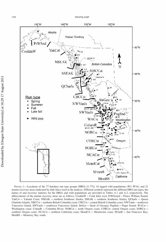
FIGURE 1.—Locations of the 77 hatchery run type groups (HRGs [1–77]), 16 tagged wild populations (W1–W16), and 21
marine recovery areas (indicated by dark lines) used in the analysis. Different symbols represent the different HRG run types; the
names of and recovery statistics for the HRGs and wild populations are provided in Tables A.1 and A.2, respectively. The
abbreviations of the marine recovery areas are as follows: CookInW ¼ Cook Inlet west; PrWSound ¼ Prince William Sound;
YakCst ¼ Yakutat Coast; NSEAK ¼ northern Southeast Alaska; SSEAK ¼ southern Southeast Alaska; QCharIs ¼ Queen
Charlotte Islands; NBCCst¼ northern British Columbia coast; CBCCst¼ central British Columbia coast; NWVanIs¼ northwest
Vancouver Island; SWVanIs ¼ southwest Vancouver Island; StrGeo ¼ Strait of Georgia; PugSnd ¼ Puget Sound; WACst ¼Washington coast; ColumR ¼ Columbia River; NORCst ¼ north Oregon coast; CORCst: central Oregon coast; SORCst ¼southern Oregon coast; NCACst ¼ northern California coast; MendCst ¼ Mendocino coast; SFranB ¼ San Francisco Bay;
MonBS¼Monterey Bay south.
150 WEITKAMP
Dow
nloa
ded
by [
Ore
gon
Stat
e U
nive
rsity
] at
16:
29 1
7 A
ugus
t 201
1

gives equal weight to all recoveries, regardless of the
year in which fish were recovered. This provided the
primary data set for the analysis: the proportion (or
percent by multiplying portions by 100) of recoveries
in each of the 21 recovery areas for each HRG.
I also estimated the weighted average marine
distance of recovery (D; travel by water only) for each
HRG j between all recovery areas in which Chinook
salmon were recovered and the recovery area j in which
their home stream enters the ocean (‘‘home recovery
area’’) as
D ¼X
i
diRij;
where diis marine distance (using great-circle distance)
between the geographic center of recovery area i and
the center of the home recovery area j, and Rij
is the
proportion of recoveries by HRG j in recovery area i,defined above. Because recovery area was the smallest
spatial scale used in this analysis, all recoveries
occurring within the home recovery area had a distance
of zero. Untransformed mean distances were compared
by release region or run type using either Mann–
Whitney test of medians (MW) followed by Bonferroni
test between pairwise groups or Kruskal Wallace (KW)
one-way analysis of variance (ANOVA) on ranks
followed by a KW multiple-comparison test (Zar
1984).
Statistical analysis of marine distributions.—I
employed three complementary multivariate techniques
to explore variation in marine distributions: (1)
nonmetric multidimensional scaling (MDS), (2) anal-
ysis of similarities (ANOSIM; a multivariate analog to
ANOVA) to test for the influence of specific factors on
ocean distributions, and (3) cluster analysis. All
analyses were run using PRIMER-E software (Clarke
and Gorley 2006). These analyses all employed
resemblance matrices constructed using pairwise
Bray–Curtis similarities (S) between each pair of
HRGs (i and j) as
Sij ¼
X
k
2 minðrik; rjkÞX
k
ðrik þ rjkÞ;
where rik
and rjk
are the proportion of recoveries in
recovery area k by HRGs i and j, respectively. In this
application, Bray–Curtis similarity ranges from 0 (no
recoveries in common) to 1 (identical recovery
patterns). Bray–Curtis similarity coefficients are widely
used in ecological studies because they are unaffected
by changes in scale (e.g., using percent or proportions)
or the number of variables (recovery areas) used, and
produces a value of zero when both values being
compared are zero (joint absence problem; Clarke
1993; Legendre and Legendre 1998). Proportions were
deliberately not transformed so that variation in the
original data were retained, although analyses con-
ducted with log or square root transformations
produced similar results.
The MDS is a ranking technique based on a set of
similarity coefficients that places points in two- (2-D)
or three-dimensional (3-D) MDS space in relation to
their similarity (i.e., points farther apart are less similar
than those closer together). Unlike multivariate AN-
OVA, MDS does not require data to be normally
distributed and is better suited for the large number of
variables employed here (21 recovery areas; Clarke
1993). The MDS uses an iterative process to find the
best (minimum) solution; therefore, each run used 25
iterations with random starting locations. Minimum
stress (a measure of agreement between the ranks of
similarities and distances in 2-D [or 3-D] MDS space)
was attained in multiple iterations of each run, while
multiple runs of each data set produced similar
configurations, suggesting true minimum solutions
were attained with this method.
As applied here, the ANOSIM is a permutation
procedure used to test whether particular groups of
HRGs were more similar to each other with respect to
recovery patterns than would be expected strictly by
chance (Clarke 1993). The groups of interest were
those based on release region and run type. The
procedure produces a global R-statistic that typically
ranges from 0 (no separation of groups) to 1 (complete
separation of groups), although negative values
(indicating no separation) are possible (Clarke 1993).
Finally, to evaluate how release region influences
recovery patterns without the added influence of run
type, I analyzed only fall run type HRGs using
hierarchical agglomerative clustering based on group-
averaging linkages. The cluster analysis included the
similarity profile (SIMPROF) test, which determines
the significance of each node of the cluster by
permutation (Clarke 1993).
Comparison of hatchery and wild marine distribu-tions.—Because most salmon tagged with CWTs are
hatchery reared, yet hatchery-reared fish are known to
vary from their wild counterparts in many important
ways (NRC 1996; Quinn 2005), I explored whether
recovery patterns for HRGs were similar to wild
salmon from the same release region. This evaluation
used the methods described above for HRGs (e.g.,
same recovery areas, years of interest, release criteria,
marine recovery metrics). However, because relatively
few wild Chinook salmon have been tagged and
recovered, I included populations that had fewer than
1,000 recoveries and included wild fish that were
MARINE DISTRIBUTIONS OF CHINOOK SALMON 151
Dow
nloa
ded
by [
Ore
gon
Stat
e U
nive
rsity
] at
16:
29 1
7 A
ugus
t 201
1
trapped, tagged, and released from multiple tributaries
within each river basin (Table A.2).
Marine distributions of wild populations were
compared to HRGs at two spatial scales. At fine
spatial scales, I calculated Bray–Curtis similarity
coefficients between each wild population and the
nearest HRG with the same run type to quantify the
similarity between the two. At large spatial scales, all
wild populations were included with all HRGs in an
MDS plot to determine whether wild populations were
similar to hatchery populations from the same release
region, regardless of exact geographic location or run
type.
Marine distributions by year and ocean age.—I
conducted two secondary analyses to explore how
marine distributions varied by year and by ocean age
(ocean age ¼ recovery year – release year). These
analyses were restricted to HRGs used in the main
analysis that had at least 100 estimated recoveries in
each of 10 years (1979–1994 only) or at least four
ocean ages (1–5); too few tagged Chinook salmon were
recovered at ocean age 0 to analyze. For each HRG
used in these analyses, I calculated the proportion of
recoveries in each recovery area and mean distance of
recovery (both described previously) for each year or
ocean age that had a minimum of 100 estimated
recoveries.
Bray–Curtis similarity coefficients were calculated
between years or ocean ages, both within and between
HRGs. Differences in similarity coefficients between
years or ocean ages within HRGs were evaluated using
either nonparametric (KW tests) or parametric one-way
ANOVAs on untransformed data, as appropriate (Zar
1984). This analysis included examination of whether
particular years may have influenced recovery patterns
coastwide (as might be expected from ocean-scale El
Ni~no or La Ni~na events), leading to consistently low
mean similarities with other years. These analyses only
considered similarities calculated within HRGs be-
tween years (i.e., no between-HRG similarities were
included). I also used pairwise Bray–Curtis similarities
as a basis for MDS, ANOSIM, and cluster analyses to
explore variation associated with year or age, using the
methods described for the primary analysis above.
Variation in mean distance by year was evaluated
using coefficient of variation (CV ¼ 100 3 SD/mean)
corrected for small sample sizes (Sokal and Rohlf
1995). Variation in CV by run type was evaluated by
one-way ANOVA on untransformed data, which met
all normality and variance assumptions (Zar 1984). The
effects of ocean age on mean distance of recovery was
explored by converting distance at each age into
standardized anomalies so that mean distances by age
for each HRG had a mean of zero and SD equal to 1.
These were compared across HRGs by ocean age using
KW tests (Zar 1984).
ResultsRecovery Statistics
This analysis was based on an estimated 620,275
hatchery Chinook salmon recovered in coastal waters
of the eastern North Pacific. These tagged salmon
represented 3,375 CWT release groups and 77 HRGs
from Alaska (5), British Columbia (29), Washington
(25), Oregon (12), and California (6; Figure 1). Over
half of the HRGs consisted of fall run types (42), with
lesser numbers of spring (19), summer (14), and late
fall (upriver bright) (2) run types (Table A.1). The
analysis also employed recoveries of an estimated
11,982 wild Chinook salmon that were tagged as
smolts in 16 rivers in Alaska (4), British Columbia (2),
Washington (3), Oregon (1) and California (6; Figure
1; Table A.2). Like hatchery Chinook salmon, most
wild release groups consisted of fall run types (56%),
followed by spring (31%) and summer (13%) run
types. On average, each recovery area recovered an
estimated 29,537 hatchery and 569 wild tagged fish,
representing 47 HRGs and 7 wild populations,
respectively (Table A.3).
Hatchery Location and Marine Distribution Patterns
Marine distribution patterns for the 77 HRGs
indicate a clear latitudinal cline: tagged Chinook
salmon released from northern hatcheries had more
northern distributions than those from southern hatch-
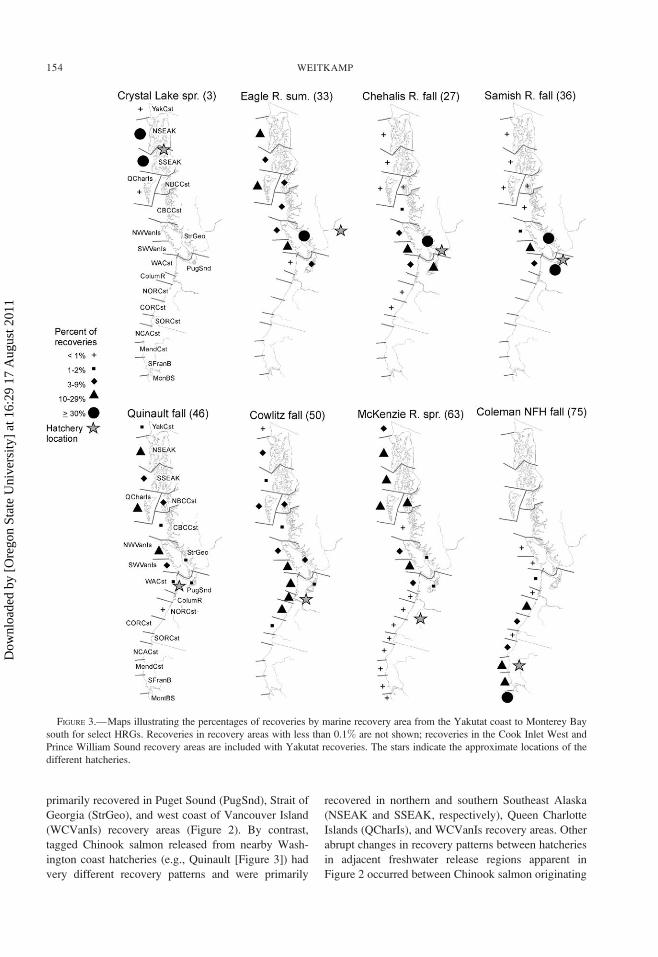
eries (Figures 2, 3). However, the distribution of fish
across recovery areas followed three broad patterns
based on release region: (1) Chinook salmon from
Alaskan hatcheries (HRGs 1–5) were largely recovered
in Alaska, few recoveries occurring south of Alaska;
(2) salmon originating from hatcheries in northern
British Columbia to the Oregon coast (HRGs 6–69)
were widely dispersed and recovered from the home
recovery area (in which the natal stream enters the
ocean) north to Southeast Alaska; and (3) Chinook
salmon from hatcheries in southern Oregon and
California (HRGs 70–77) were rarely caught north of
the Columbia River (ColumR) recovery area. These
southern hatcheries also had the highest number of
recoveries south of the home recovery area (Figures 2,
3).
Within this second group, recovery patterns were
also apparent at finer spatial scales such that Chinook
salmon released from a particular geographic region
generally shared a common recovery pattern which was
distinct from that of adjacent regions. For example,
most Chinook salmon released from Puget Sound
hatcheries (e.g., Samish River [Figure 3]) were
152 WEITKAMP
Dow
nloa
ded
by [
Ore
gon
Stat
e U
nive
rsity
] at
16:
29 1
7 A
ugus
t 201
1

FIGURE 2.—Recovery patterns for coded-wire-tagged Chinook salmon by HRG, arranged by geographic region from north
(top) to south (bottom). Each horizontal bar represents the percentages of recoveries in the 21 marine recovery areas for a single
HRG; recovery area abbreviations and boundaries are provided in Figure 1. Run timing (RT) and HRG numbers are indicated to
the left of the bar chart. See Figure 1 for HRG locations and Table A.1 for HRG names and recovery statistics.
MARINE DISTRIBUTIONS OF CHINOOK SALMON 153
Dow
nloa
ded
by [
Ore
gon
Stat
e U
nive
rsity
] at
16:
29 1
7 A
ugus
t 201
1
primarily recovered in Puget Sound (PugSnd), Strait of
Georgia (StrGeo), and west coast of Vancouver Island
(WCVanIs) recovery areas (Figure 2). By contrast,
tagged Chinook salmon released from nearby Wash-
ington coast hatcheries (e.g., Quinault [Figure 3]) had
very different recovery patterns and were primarily
recovered in northern and southern Southeast Alaska
(NSEAK and SSEAK, respectively), Queen Charlotte
Islands (QCharIs), and WCVanIs recovery areas. Other
abrupt changes in recovery patterns between hatcheries
in adjacent freshwater release regions apparent in
Figure 2 occurred between Chinook salmon originating
FIGURE 3.—Maps illustrating the percentages of recoveries by marine recovery area from the Yakutat coast to Monterey Bay
south for select HRGs. Recoveries in recovery areas with less than 0.1% are not shown; recoveries in the Cook Inlet West and
Prince William Sound recovery areas are included with Yakutat recoveries. The stars indicate the approximate locations of the
different hatcheries.
154 WEITKAMP
Dow
nloa
ded
by [
Ore
gon
Stat
e U
nive
rsity
] at
16:
29 1
7 A
ugus
t 201
1
from (1) southeast Alaska and northern British
Columbia; (2) upper Fraser River, Puget Sound, and
the Washington coast, and (3) the Oregon coast,
southern Oregon–northern California, and the Central
Valley.
Salmon from the same release region but with
different run types also had different marine distribu-
tions in many cases (Figures 2, 3). For example, the
three spring Chinook salmon HRGs from the Will-
amette River (62–64; McKenzie River [Figure 3]) had
similar recovery patterns and were largely caught in
NSEAK, SSEAK, QCharIs, and northern British
Columbia coast (NBCCst) recovery areas. By contrast,
the only fall Chinook salmon from the Willamette
River (Stayton Pond, 65) was largely restricted to
WCVanIs and Washington coast (WACst) recovery
areas (Figure 2). Similarly, most recoveries of fall
Chinook salmon from the lower Fraser River (HRGs
27–28; Chehalis River [Figure 3]) were in or near the
home recovery area (StrGeo, PugSnd, WCVanIs),
while Upper Fraser River summer Chinook salmon
(HRGs 29, 32–34; Eagle River [Figure 3]) also
included recoveries in NSEAK, SSEAK, and NBCCst
recovery areas.
This tendency for spring or summer run types to be
recovered farther from the home recovery area than fall
run types from the same region is also apparent in
mean recovery distance, which was significantly lower
in fall-type HRGs (mean¼ 225 km) than either spring
(380 km) or summer (342 km) run types from the same
region (KW H � 6.7; P , 0.05). In other cases, there
was little variation in recovery patterns for different run
types within common release regions; recovery patterns
for spring and summer Chinook salmon from northern
British Columbia were quite similar, as were those for
spring, summer, and fall Chinook salmon from Puget
Sound, and spring and fall Chinook salmon from
southern Oregon–northern California (Figure 2).
Several HRGs also appeared to have distribution
patterns that differed from the region-specific pattern
(Figure 2), perhaps reflecting transitional distributions.
In particular, both the Elwha (43) and Elk River (69)
had recovery patterns that were intermediate between
the release region in which they are located (Puget
Sound [35–43] and Oregon coast [66–69], respective-
ly) and adjacent regions (Washington coast and
southern Oregon, respectively). Chinook salmon re-
leased from Columbia River hatcheries (including the
Snake and Willamette rivers; HRGs 49–65) also
showed considerable variation in recovery patterns,
mainly due to the proportion of recoveries in NSEAK
and SSEAK recovery areas. However, this variation
appeared to be largely independent of either run type or
hatchery location within the basin (Figure 2).
Statistical Analysis of Hatchery Marine Distributions
Variation in recovery patterns between HRGs was
explored using MDS, ANOSIM, and comparisons of
pairwise Bray–Curtis similarities and confirmed many
of the patterns observed in Figures 2 and 3, discussed
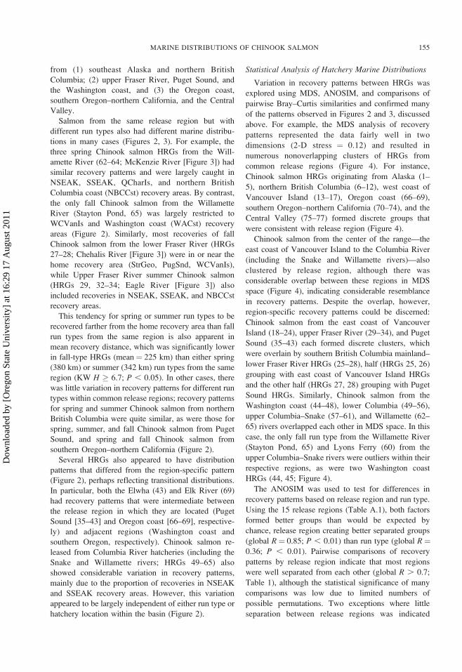
above. For example, the MDS analysis of recovery
patterns represented the data fairly well in two
dimensions (2-D stress ¼ 0.12) and resulted in
numerous nonoverlapping clusters of HRGs from
common release regions (Figure 4). For instance,
Chinook salmon HRGs originating from Alaska (1–
5), northern British Columbia (6–12), west coast of
Vancouver Island (13–17), Oregon coast (66–69),
southern Oregon–northern California (70–74), and the
Central Valley (75–77) formed discrete groups that
were consistent with release region (Figure 4).
Chinook salmon from the center of the range—the
east coast of Vancouver Island to the Columbia River
(including the Snake and Willamette rivers)—also
clustered by release region, although there was
considerable overlap between these regions in MDS
space (Figure 4), indicating considerable resemblance
in recovery patterns. Despite the overlap, however,
region-specific recovery patterns could be discerned:
Chinook salmon from the east coast of Vancouver
Island (18–24), upper Fraser River (29–34), and Puget
Sound (35–43) each formed discrete clusters, which
were overlain by southern British Columbia mainland–
lower Fraser River HRGs (25–28), half (HRGs 25, 26)
grouping with east coast of Vancouver Island HRGs
and the other half (HRGs 27, 28) grouping with Puget
Sound HRGs. Similarly, Chinook salmon from the
Washington coast (44–48), lower Columbia (49–56),
upper Columbia–Snake (57–61), and Willamette (62–
65) rivers overlapped each other in MDS space. In this
case, the only fall run type from the Willamette River
(Stayton Pond, 65) and Lyons Ferry (60) from the
upper Columbia–Snake rivers were outliers within their
respective regions, as were two Washington coast
HRGs (44, 45; Figure 4).
The ANOSIM was used to test for differences in
recovery patterns based on release region and run type.
Using the 15 release regions (Table A.1), both factors
formed better groups than would be expected by
chance, release region creating better separated groups
(global R¼ 0.85; P , 0.01) than run type (global R¼0.36; P , 0.01). Pairwise comparisons of recovery
patterns by release region indicate that most regions
were well separated from each other (global R . 0.7;
Table 1), although the statistical significance of many
comparisons was low due to limited numbers of
possible permutations. Two exceptions where little
separation between release regions was indicated
MARINE DISTRIBUTIONS OF CHINOOK SALMON 155
Dow
nloa
ded
by [
Ore
gon
Stat
e U
nive
rsity
] at
16:
29 1
7 A
ugus
t 201
1
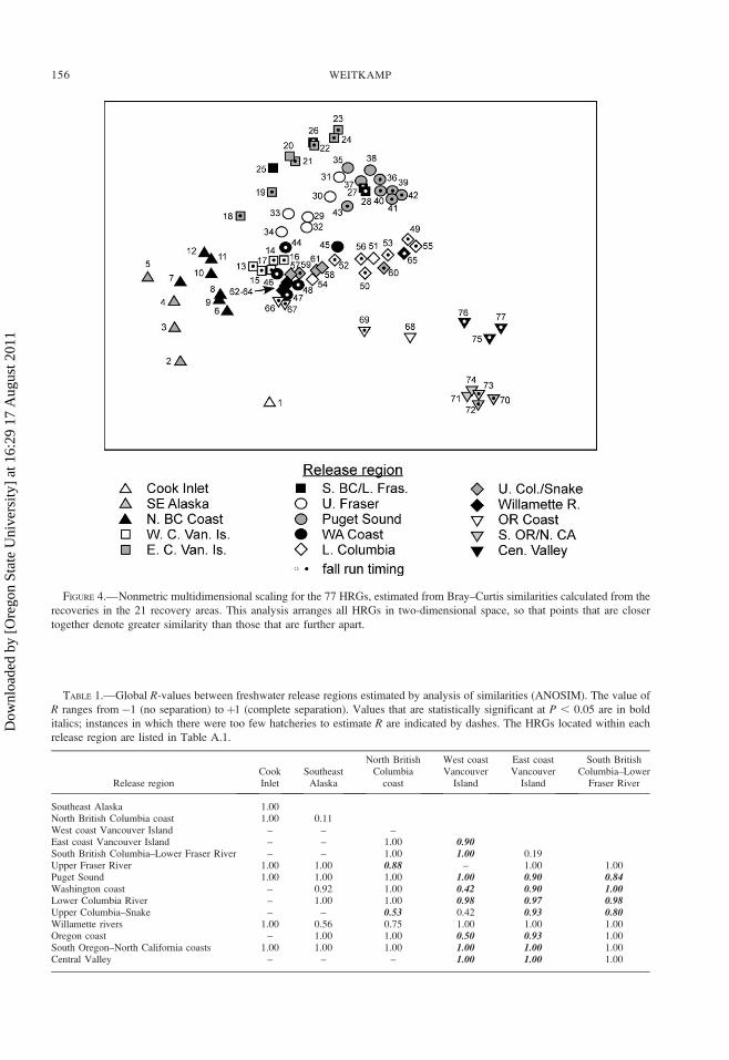
TABLE 1.—Global R-values between freshwater release regions estimated by analysis of similarities (ANOSIM). The value of
R ranges from�1 (no separation) to þ1 (complete separation). Values that are statistically significant at P , 0.05 are in bold
italics; instances in which there were too few hatcheries to estimate R are indicated by dashes. The HRGs located within each
release region are listed in Table A.1.
Release regionCookInlet
SoutheastAlaska
North BritishColumbia
coast
West coastVancouver
Island
East coastVancouver
Island
South BritishColumbia–Lower
Fraser River
Southeast Alaska 1.00North British Columbia coast 1.00 0.11West coast Vancouver Island – – –East coast Vancouver Island – – 1.00 0.90South British Columbia–Lower Fraser River – – 1.00 1.00 0.19Upper Fraser River 1.00 1.00 0.88 – 1.00 1.00Puget Sound 1.00 1.00 1.00 1.00 0.90 0.84Washington coast – 0.92 1.00 0.42 0.90 1.00Lower Columbia River – 1.00 1.00 0.98 0.97 0.98Upper Columbia–Snake – – 0.53 0.42 0.93 0.80Willamette rivers 1.00 0.56 0.75 1.00 1.00 1.00Oregon coast – 1.00 1.00 0.50 0.93 1.00South Oregon–North California coasts 1.00 1.00 1.00 1.00 1.00 1.00Central Valley – – – 1.00 1.00 1.00
FIGURE 4.—Nonmetric multidimensional scaling for the 77 HRGs, estimated from Bray–Curtis similarities calculated from the
recoveries in the 21 recovery areas. This analysis arranges all HRGs in two-dimensional space, so that points that are closer
together denote greater similarity than those that are further apart.
156 WEITKAMP
Dow
nloa
ded
by [
Ore
gon
Stat
e U
nive
rsity
] at
16:
29 1
7 A
ugus
t 201
1
despite high statistical power were between the east
coast of Vancouver Island and southern British
Columbia mainland–lower Fraser River (R ¼ 0.19),
and upper Fraser River and Puget Sound regions (R¼0.26; Table 1); this is consistent with overlap between
these HRGs in the MDS plot (Figure 4).
By run type, ANOSIM indicated that spring runs had
distinct recovery patterns from both summer and fall
runs (R¼ 0.38; P , 0.05), while summer and fall run
types did not form well-separated groups (R¼ 0.10; P
. 0.10). I also used Bray–Curtis similarities calculated
between all pairs of HRGs (n ¼ 2,926) to explore
variation in recovery patterns by run type within
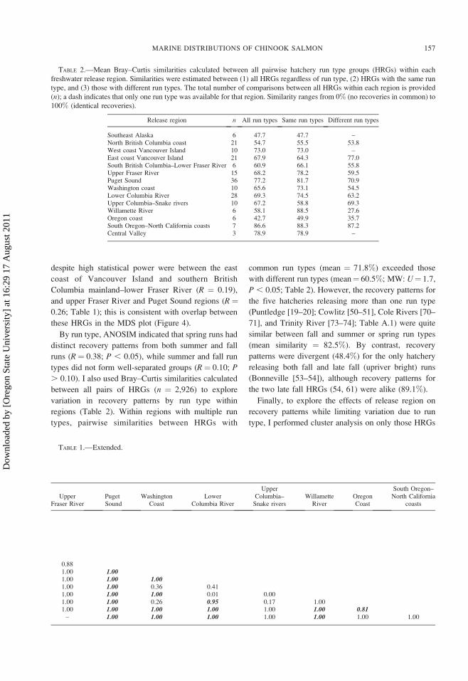
regions (Table 2). Within regions with multiple run
types, pairwise similarities between HRGs with
common run types (mean ¼ 71.8%) exceeded those
with different run types (mean¼ 60.5%; MW: U¼ 1.7,
P , 0.05; Table 2). However, the recovery patterns for
the five hatcheries releasing more than one run type
(Puntledge [19–20]; Cowlitz [50–51], Cole Rivers [70–
71], and Trinity River [73–74]; Table A.1) were quite
similar between fall and summer or spring run types
(mean similarity ¼ 82.5%). By contrast, recovery
patterns were divergent (48.4%) for the only hatchery
releasing both fall and late fall (upriver bright) runs
(Bonneville [53–54]), although recovery patterns for
the two late fall HRGs (54, 61) were alike (89.1%).
Finally, to explore the effects of release region on
recovery patterns while limiting variation due to run
type, I performed cluster analysis on only those HRGs
TABLE 2.—Mean Bray–Curtis similarities calculated between all pairwise hatchery run type groups (HRGs) within each
freshwater release region. Similarities were estimated between (1) all HRGs regardless of run type, (2) HRGs with the same run
type, and (3) those with different run types. The total number of comparisons between all HRGs within each region is provided
(n); a dash indicates that only one run type was available for that region. Similarity ranges from 0% (no recoveries in common) to
100% (identical recoveries).
Release region n All run types Same run types Different run types
Southeast Alaska 6 47.7 47.7 –North British Columbia coast 21 54.7 55.5 53.8West coast Vancouver Island 10 73.0 73.0 –East coast Vancouver Island 21 67.9 64.3 77.0South British Columbia–Lower Fraser River 6 60.9 66.1 55.8Upper Fraser River 15 68.2 78.2 59.5Puget Sound 36 77.2 81.7 70.9Washington coast 10 65.6 73.1 54.5Lower Columbia River 28 69.3 74.5 63.2Upper Columbia–Snake rivers 10 67.2 58.8 69.3Willamette River 6 58.1 88.5 27.6Oregon coast 6 42.7 49.9 35.7South Oregon–North California coasts 7 86.6 88.3 87.2Central Valley 3 78.9 78.9 –
TABLE 1.—Extended.
UpperFraser River
PugetSound
WashingtonCoast
LowerColumbia River
UpperColumbia–
Snake riversWillamette
RiverOregonCoast
South Oregon–North California
coasts
0.881.00 1.001.00 1.00 1.001.00 1.00 0.36 0.411.00 1.00 1.00 0.01 0.001.00 1.00 0.26 0.95 0.17 1.001.00 1.00 1.00 1.00 1.00 1.00 0.81
– 1.00 1.00 1.00 1.00 1.00 1.00 1.00
MARINE DISTRIBUTIONS OF CHINOOK SALMON 157
Dow
nloa
ded
by [
Ore
gon
Stat
e U
nive
rsity
] at
16:
29 1
7 A
ugus
t 201
1

that contained fall Chinook salmon. The resulting
dendrogram contains eight distinct clusters (labeled A–
H in Figure 5) with strong correspondence to release
location. With only two exceptions, all clusters
contained fall Chinook salmon from a single geo-
graphic area, such as Puget Sound (cluster C),
Columbia River (cluster E), or the Central Valley
(cluster H). The two exceptions included HRGs that
were either from coastal areas (cluster B) or HRGs
from adjacent regions (cluster F). In addition, one HRG
identified as transitional in Figure 2 (Elk River [69])
formed its own cluster (A), while another transitional
HRG (Elwha [43]) grouped with other Puget Sound
hatcheries (Figure 5). Like the MDS and ANOSIM
analyses, this analysis confirms that release region
dominates distribution patterns with generally abrupt
transitions between regions.
Comparison of Hatchery and Wild MarineDistributions
Bray–Curtis similarities were calculated between the
16 tagged wild Chinook salmon populations and the
nearest hatchery with the same run type. High mean
Bray–Curtis similarity (average ¼ 75.3%; Table 3)
FIGURE 5.—Dendrogram resulting from a cluster analysis of 42 fall Chinook salmon HRGs based on CWT recovery patterns,
using Bray–Curtis similarities and group-average linkage. The similarity profile permutation test was used to determine that eight
clusters (A–H) were statistically valid. The region of each HRG is provided by name and symbol as in Figure 4.
158 WEITKAMP
Dow
nloa
ded
by [
Ore
gon
Stat
e U
nive
rsity
] at
16:
29 1
7 A
ugus
t 201
1
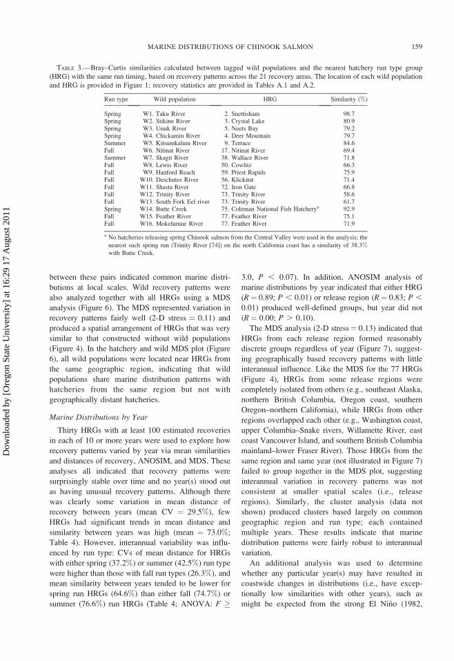
between these pairs indicated common marine distri-
butions at local scales. Wild recovery patterns were
also analyzed together with all HRGs using a MDS
analysis (Figure 6). The MDS represented variation in
recovery patterns fairly well (2-D stress ¼ 0.11) and
produced a spatial arrangement of HRGs that was very
similar to that constructed without wild populations
(Figure 4). In the hatchery and wild MDS plot (Figure
6), all wild populations were located near HRGs from
the same geographic region, indicating that wild
populations share marine distribution patterns with
hatcheries from the same region but not with
geographically distant hatcheries.
Marine Distributions by Year
Thirty HRGs with at least 100 estimated recoveries
in each of 10 or more years were used to explore how
recovery patterns varied by year via mean similarities
and distances of recovery, ANOSIM, and MDS. These
analyses all indicated that recovery patterns were
surprisingly stable over time and no year(s) stood out
as having unusual recovery patterns. Although there
was clearly some variation in mean distance of
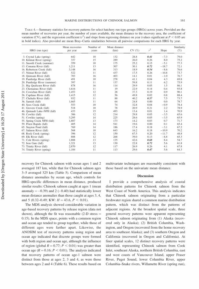
recovery between years (mean CV ¼ 29.5%), few
HRGs had significant trends in mean distance and
similarity between years was high (mean ¼ 73.0%;
Table 4). However, interannual variability was influ-
enced by run type: CVs of mean distance for HRGs
with either spring (37.2%) or summer (42.5%) run type
were higher than those with fall run types (26.3%), and
mean similarity between years tended to be lower for
spring run HRGs (64.6%) than either fall (74.7%) or
summer (76.6%) run HRGs (Table 4; ANOVA: F �
3.0, P , 0.07). In addition, ANOSIM analysis of
marine distributions by year indicated that either HRG
(R¼ 0.89; P , 0.01) or release region (R¼ 0.83; P ,
0.01) produced well-defined groups, but year did not
(R ¼ 0.00; P . 0.10).
The MDS analysis (2-D stress¼ 0.13) indicated that
HRGs from each release region formed reasonably
discrete groups regardless of year (Figure 7), suggest-
ing geographically based recovery patterns with little
interannual influence. Like the MDS for the 77 HRGs
(Figure 4), HRGs from some release regions were
completely isolated from others (e.g., southeast Alaska,
northern British Columbia, Oregon coast, southern
Oregon–northern California), while HRGs from other
regions overlapped each other (e.g., Washington coast,
upper Columbia–Snake rivers, Willamette River, east
coast Vancouver Island, and southern British Columbia
mainland–lower Fraser River). Those HRGs from the
same region and same year (not illustrated in Figure 7)
failed to group together in the MDS plot, suggesting
interannual variation in recovery patterns was not
consistent at smaller spatial scales (i.e., release
regions). Similarly, the cluster analysis (data not
shown) produced clusters based largely on common
geographic region and run type; each contained
multiple years. These results indicate that marine
distribution patterns were fairly robust to interannual
variation.
An additional analysis was used to determine
whether any particular year(s) may have resulted in
coastwide changes in distributions (i.e., have excep-
tionally low similarities with other years), such as
might be expected from the strong El Ni~no (1982,
TABLE 3.—Bray–Curtis similarities calculated between tagged wild populations and the nearest hatchery run type group
(HRG) with the same run timing, based on recovery patterns across the 21 recovery areas. The location of each wild population
and HRG is provided in Figure 1; recovery statistics are provided in Tables A.1 and A.2.
Run type Wild population HRG Similarity (%)
Spring W1. Taku River 2. Snettisham 98.7Spring W2. Stikine River 3. Crystal Lake 80.9Spring W3. Unuk River 5. Neets Bay 79.2Spring W4. Chickamin River 4. Deer Mountain 79.7Summer W5. Kitsumkalum River 9. Terrace 84.6Fall W6. Nitinat River 17. Nitinat River 69.4Summer W7. Skagit River 38. Wallace River 71.8Fall W8. Lewis River 50. Cowlitz 66.3Fall W9. Hanford Reach 59. Priest Rapids 75.9Fall W10. Deschutes River 56. Klickitat 71.4Fall W11. Shasta River 72. Iron Gate 66.8Fall W12. Trinity River 73. Trinity River 58.6Fall W13. South Fork Eel river 73. Trinity River 61.7Spring W14. Butte Creek 75. Coleman National Fish Hatcherya 92.9Fall W15. Feather River 77. Feather River 75.1Fall W16. Mokelumne River 77. Feather River 71.9
a No hatcheries releasing spring Chinook salmon from the Central Valley were used in the analysis; the
nearest such spring run (Trinity River [74]) on the north California coast has a similarity of 38.3%with Butte Creek.
MARINE DISTRIBUTIONS OF CHINOOK SALMON 159
Dow
nloa
ded
by [
Ore
gon
Stat
e U
nive
rsity
] at
16:
29 1
7 A
ugus
t 201
1

1983) or La Ni~na (1988, 1989) events. The results
indicated that although mean similarities between years
1979–1994 were statistically different (KW: H¼ 40.7,
P , 0.01), the difference was caused by 1991 having
higher mean similarity with other years (average ¼76.9%) than the years 1980, 1981, 1983, 1984, and
1993 (70.5–72.2%). Apparently, 1991 was a particu-
larly ‘‘normal’’ year coastwide with respect to Chinook
salmon marine distributions (and ocean conditions in
general; Beamish et al. 2000; Chavez et al. 2003;
Lehodey et al. 2006), while other years (1980, 1981,
1983, 1984, 1993) were less so, but were not
consistently different from other years.
Two region-specific trends in distance over time
(Table 4) can be explained by changes in fishing effort.
The positive trend in distance for southern Oregon–
northern California HRGs (70–74) was consistent with
decreased Chinook salmon landings in northern
California and extreme southern Oregon during the
late 1980s and early 1990s (PFMC 2009), leading to
proportionally higher catches in Oregon recovery areas
and, therefore, greater mean distances for these HRGs.
In the second case, mean distances for west coast
Vancouver Island HRGs (13, 16, 17) decreased due to
increasing proportional recoveries in WCVanIs and
decreasing recoveries in recovery areas north of
Vancouver Island (NSEAK, SSEAK, NBCCst). Al-
though this trend occurred while total landings off
Vancouver Island declined by 30%, west coast
Vancouver Island tidal sport landings increased
fivefold from 1979 to 1994 (PSC 2005), suggesting
these local stocks may have been particularly vulner-
able to these ‘‘inshore’’ fisheries.
Marine Distributions by Ocean Age
Differences in marine recovery patterns by ocean
age were evaluated for 29 HRGs (Table 5) using
comparisons of Bray–Curtis similarities and mean
distances, and ANOSIM and MDS. All analyses
indicate that recovery patterns varied by ocean age,
younger fish generally being caught closer to the home
stream than older fish. For example, mean distance of
FIGURE 6.—Nonmetric multidimensional scaling for the 77 HRGs and 16 wild populations based on the recoveries in the 21
recovery areas.
160 WEITKAMP
Dow
nloa
ded
by [
Ore
gon
Stat
e U
nive
rsity
] at
16:
29 1
7 A
ugus
t 201
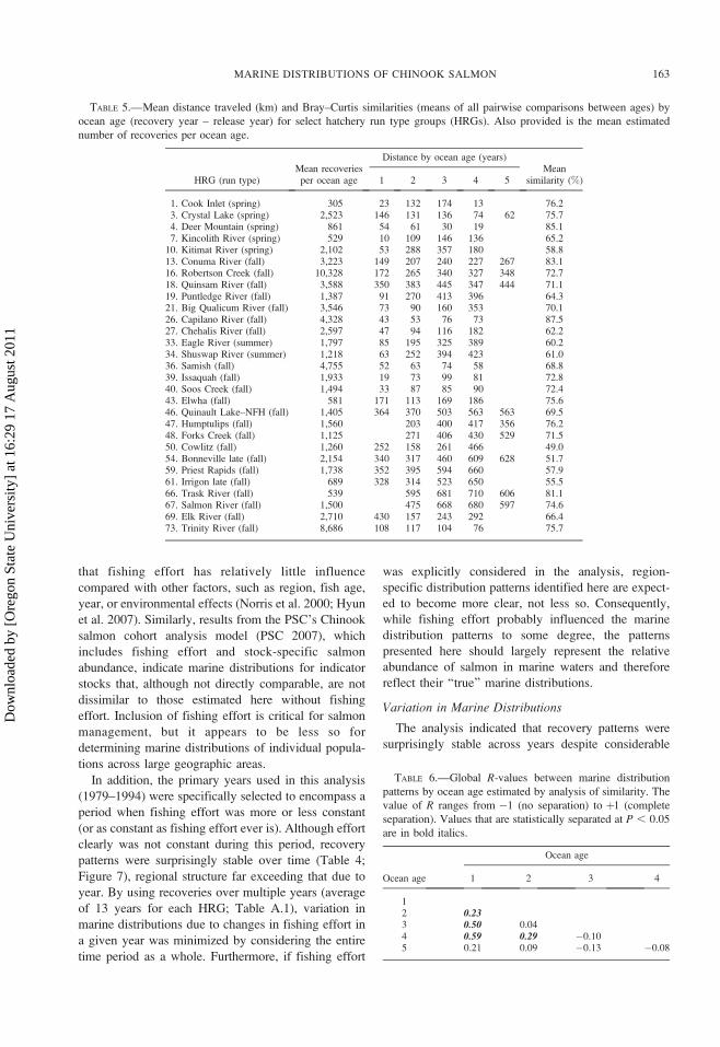
1
recovery for Chinook salmon with ocean ages 1 and 2
averaged 187 km, while that for Chinook salmon ages
3–5 averaged 325 km (Table 5). Comparison of mean
distance anomalies by ocean age, which controls for
HRG-specific differences in mean distance, produced
similar results: Chinook salmon caught at ages 1 (mean
anomaly¼�0.39) and 2 (�0.40) had statistically lower
mean distance anomalies than those caught at ages 3, 4,
and 5 (0.32–0.49; KW: H ¼ 43.6, P , 0.01).
The MDS analysis showed considerable variation in
age-based recovery patterns by release region (data not
shown), although the fit was reasonable (2-D stress ¼0.15). In the MDS space, points with a common region
and ocean age tended to group together, while those of
different ages were farther apart. Likewise, the
ANOSIM test of recovery patterns using region and
ocean age indicated that discrete groups were formed
with both region and ocean age, although the influence
of region (global R¼ 0.77; P , 0.01) was greater than
ocean age (R¼ 0.16; P , 0.01). The analysis indicated
that recovery patterns of ocean age-1 salmon were
distinct from those at ages 2, 3 and 4, as were those
between ages 2 and 4 (Table 6). These results based on
multivariate techniques are reasonably consistent with
those based on the univariate mean distance.
Discussion
I provide a comprehensive analysis of coastal
distribution patterns for Chinook salmon from the
West Coast of North America. This analysis indicates
that Chinook salmon originating from a particular
freshwater region shared a common marine distribution
pattern, which was distinct from the patterns of
adjacent regions. At the broadest spatial scale, three
general recovery patterns were apparent representing
Chinook salmon originating from (1) Alaska (recov-
ered only in Alaska); (2) British Columbia, Wash-
ington, and Oregon (recovered from the home recovery
area to southeast Alaska); and (3) southern Oregon and
California (recovered in Oregon and California). At
finer spatial scales, 12 distinct recovery patterns were
identified, representing Chinook salmon from Cook
Inlet, southeast Alaska, northern British Columbia, east
and west coasts of Vancouver Island, upper Fraser
River, Puget Sound, lower Columbia River, upper
Columbia–Snake rivers, Willamette River (spring run),
TABLE 4.—Summary statistics for recovery patterns for select hatchery run type groups (HRGs) across years. Provided are the
mean number of recoveries per year, the number of years available, the mean distance to the recovery area, the coefficient of
variation (CV), and the regression coefficient (r2) and slope from regressing distance on year (values significant at P , 0.05 are
in bold italics). Also provided are mean Bray–Curtis similarities between all pairwise comparisons for each HRG by year.
HRG (run type)Mean recoveries
per yearNumber of
yearsMean distance
(km) CV (%) r2 SlopeSimilarity
(%)
3. Crystal Lake (spring) 642 10 132 28.8 0.41 �7.3 79.010. Kitimat River (spring) 337 15 289 26.0 0.26 8.0 75.211. Snootli Creek (summer) 359 10 175 25.2 0.15 �5.1 77.313. Conuma River (fall) 1,211 13 307 30.1 0.72 �18.7 72.116. Robertson Creek (fall) 3,148 16 313 18.9 0.54 �8.6 76.617. Nitinat River (fall) 522 11 437 17.5 0.26 �10.8 73.718. Quinsam River (fall) 703 16 403 14.1 0.01 �1.0 76.719. Puntledge River (fall) 491 10 278 41.1 0.04 4.3 69.820. Puntledge River (summer) 397 11 137 59.8 0.11 6.2 75.921. Big Qualicum River (fall) 878 16 114 29.9 0.05 1.5 86.123. Chemainus River (fall) 1,616 11 19 22.9 0.14 0.4 93.824. Cowichan River (fall) 1,453 12 28 37.3 0.19 0.9 90.126. Capilano River (fall) 1,415 12 56 49.8 0.02 0.8 88.427. Chehalis River (fall) 932 11 88 40.2 0.57 7.5 73.736. Samish (fall) 1,665 11 64 24.8 0.00 0.0 78.740. Soos Creek (fall) 553 10 74 32.8 0.04 �0.9 78.441. Grovers Creek (fall) 518 10 78 20.9 0.21 2.2 78.946. Quinault Lake–NFH (fall) 433 15 493 13.4 0.01 1.4 70.950. Cowlitz (fall) 386 12 214 29.8 0.05 �3.5 65.651. Cowlitz (spring) 3,295 14 225 28.6 0.05 �3.5 65.955. Spring Creek NFH (fall) 1,887 13 173 14.2 0.03 0.7 71.759. Priest Rapids (fall) 405 14 541 19.6 0.00 0.1 65.465. Stayton Pond (fall) 769 14 186 17.4 0.18 �3.1 67.267. Salmon River (fall) 568 10 643 16.2 0.18 �10.9 70.268. Rock Creek (spring) 396 12 150 67.5 0.20 �11.7 48.869. Elk River (fall) 888 12 268 39.0 0.13 �8.8 65.371. Cole Rivers (spring) 1,888 13 135 42.6 0.68 8.4 54.772. Iron Gate (fall) 1,321 13 130 22.8 0.72 5.6 61.873. Trinity River (fall) 2,870 12 117 26.9 0.26 4.1 67.874. Trinity River (spring) 1,184 11 113 29.6 0.47 5.6 64.3
MARINE DISTRIBUTIONS OF CHINOOK SALMON 161
Dow
nloa
ded
by [
Ore
gon
Stat
e U
nive
rsity
] at
16:
29 1
7 A
ugus
t 201
1

Oregon coast, southern Oregon–northern California,
and the Central Valley (Figures 2, 4). Recovery
patterns for Chinook salmon from the southern British
Columbia mainland–lower Fraser River and Washing-
ton coast were less distinct and displayed considerable
overlap with marine distributions of adjacent release
regions.
These patterns are familiar to salmon managers who
use distributional differences at even finer spatial and
temporal scales to target fisheries on particular stocks
while avoiding others. For example, in 2008 ocean
fisheries for Chinook salmon were closed from Cape
Falcon (the dividing line between the north Oregon
coast [NORCst] and ColumR recovery areas) to the
U.S.–Mexico border to minimize ocean harvest of
Central Valley Chinook salmon (PFMC 2009). Not
surprisingly, my analysis indicated that 94% of
recoveries of Central Valley HRGs (75–77; Coleman
NFH [Figure 3]) occurred within this area (NORCst to
Monterey Bay South recovery areas), suggesting the
closure was highly effective. While managers are
typically focused on marine distributions of particular
stocks, however, this analysis included populations
along the entire West Coast of North America.
Assumptions Underlying the Analysis
This analysis assumes that the number of Chinook
salmon with CWTs recovered in a particular recovery
area reflects the abundance of tagged fish in that area
relative to other recovery areas. However, catch is a
function of both salmon abundance and fishing effort,
potentially leading to violations of the assumption if
effort is unevenly distributed in space or time. Fishing
effort was deliberately excluded from calculations of
marine recovery patterns in order to simplify the
analysis, yet its absence may bias the marine
distribution patterns or recovery distances provided
here. For example, correspondence between trends in
distance by year and changes in landings in northern
California and off the west coast of Vancouver Island
discussed above point to two examples where fishing
effort clearly influenced recovery patterns.
Despite this potentially confounding factor, howev-
er, the patterns presented here are thought to largely
reflect Chinook salmon abundance in the coastal
eastern North Pacific, with relatively minor influence
from fishing effort. Studies that have deliberately
incorporated fishing effort in estimations of marine
distributions or ocean recovery rates have demonstrated
FIGURE 7.—Nonmetric multidimensional scaling by year for select HRGs based on the recoveries in the 21 recovery areas. For
clarity, the HRG numbers and years are not shown, but the points are coded by release region.
162 WEITKAMP
Dow
nloa
ded
by [
Ore
gon
Stat
e U
nive
rsity
] at
16:
29 1
7 A
ugus
t 201
1
that fishing effort has relatively little influence
compared with other factors, such as region, fish age,
year, or environmental effects (Norris et al. 2000; Hyun
et al. 2007). Similarly, results from the PSC’s Chinook
salmon cohort analysis model (PSC 2007), which
includes fishing effort and stock-specific salmon
abundance, indicate marine distributions for indicator
stocks that, although not directly comparable, are not
dissimilar to those estimated here without fishing
effort. Inclusion of fishing effort is critical for salmon
management, but it appears to be less so for
determining marine distributions of individual popula-
tions across large geographic areas.
In addition, the primary years used in this analysis
(1979–1994) were specifically selected to encompass a
period when fishing effort was more or less constant
(or as constant as fishing effort ever is). Although effort
clearly was not constant during this period, recovery
patterns were surprisingly stable over time (Table 4;
Figure 7), regional structure far exceeding that due to
year. By using recoveries over multiple years (average
of 13 years for each HRG; Table A.1), variation in
marine distributions due to changes in fishing effort in
a given year was minimized by considering the entire
time period as a whole. Furthermore, if fishing effort
was explicitly considered in the analysis, region-
specific distribution patterns identified here are expect-
ed to become more clear, not less so. Consequently,
while fishing effort probably influenced the marine
distribution patterns to some degree, the patterns
presented here should largely represent the relative
abundance of salmon in marine waters and therefore
reflect their ‘‘true’’ marine distributions.
Variation in Marine Distributions
The analysis indicated that recovery patterns were
surprisingly stable across years despite considerable
TABLE 6.—Global R-values between marine distribution
patterns by ocean age estimated by analysis of similarity. The
value of R ranges from �1 (no separation) to þ1 (complete
separation). Values that are statistically separated at P , 0.05
are in bold italics.
Ocean age
Ocean age
1 2 3 4
12 0.233 0.50 0.044 0.59 0.29 �0.105 0.21 0.09 �0.13 �0.08
TABLE 5.—Mean distance traveled (km) and Bray–Curtis similarities (means of all pairwise comparisons between ages) by
ocean age (recovery year – release year) for select hatchery run type groups (HRGs). Also provided is the mean estimated
number of recoveries per ocean age.
HRG (run type)Mean recoveries
per ocean age
Distance by ocean age (years)Mean
similarity (%)1 2 3 4 5
1. Cook Inlet (spring) 305 23 132 174 13 76.23. Crystal Lake (spring) 2,523 146 131 136 74 62 75.74. Deer Mountain (spring) 861 54 61 30 19 85.17. Kincolith River (spring) 529 10 109 146 136 65.2
10. Kitimat River (spring) 2,102 53 288 357 180 58.813. Conuma River (fall) 3,223 149 207 240 227 267 83.116. Robertson Creek (fall) 10,328 172 265 340 327 348 72.718. Quinsam River (fall) 3,588 350 383 445 347 444 71.119. Puntledge River (fall) 1,387 91 270 413 396 64.321. Big Qualicum River (fall) 3,546 73 90 160 353 70.126. Capilano River (fall) 4,328 43 53 76 73 87.527. Chehalis River (fall) 2,597 47 94 116 182 62.233. Eagle River (summer) 1,797 85 195 325 389 60.234. Shuswap River (summer) 1,218 63 252 394 423 61.036. Samish (fall) 4,755 52 63 74 58 68.839. Issaquah (fall) 1,933 19 73 99 81 72.840. Soos Creek (fall) 1,494 33 87 85 90 72.443. Elwha (fall) 581 171 113 169 186 75.646. Quinault Lake–NFH (fall) 1,405 364 370 503 563 563 69.547. Humptulips (fall) 1,560 203 400 417 356 76.248. Forks Creek (fall) 1,125 271 406 430 529 71.550. Cowlitz (fall) 1,260 252 158 261 466 49.054. Bonneville late (fall) 2,154 340 317 460 609 628 51.759. Priest Rapids (fall) 1,738 352 395 594 660 57.961. Irrigon late (fall) 689 328 314 523 650 55.566. Trask River (fall) 539 595 681 710 606 81.167. Salmon River (fall) 1,500 475 668 680 597 74.669. Elk River (fall) 2,710 430 157 243 292 66.473. Trinity River (fall) 8,686 108 117 104 76 75.7
MARINE DISTRIBUTIONS OF CHINOOK SALMON 163
Dow
nloa
ded
by [
Ore
gon
Stat
e U
nive
rsity
] at
16:
29 1
7 A
ugus
t 201
1
variation in ocean conditions observed during 1979–
1994, including strong El Ni~no (1982–83) and La Ni~na
(1988–89) events (Trenberth 1997). These variable
ocean conditions altered marine ecosystems throughout
the northeast Pacific Ocean (e.g., Beamish et al. 2000;
Chavez et al. 2003; Lehodey et al. 2006) and
influenced Chinook salmon survival and growth
directly (Johnson 1988; Magnusson and Hilborn
2003; Wells et al. 2006). Little interannual change in
marine distributions suggest that Chinook salmon
distributions are driven to a larger degree by genetic
control of migration (Brannon and Setter 1989; Kallio-
Nyberg and Ikonen 1992) than by either local
environmental conditions (Hodgson et al. 2006) or
opportunistic foraging opportunities (Kallio-Nyberg et
al. 1999; Healey 2000). This high stability may reflect
a strategy to ‘‘spread the risk’’ in response to
unpredictable ocean conditions (Leggett 1985), result-
ing in higher survival overall than species which are
less dispersed and, therefore, more vulnerable to
catastrophic events.
In contrast, marine distribution patterns were
influenced by ocean age, and individuals that spent
longer in the ocean were recovered farther from the
home stream than those that had recently entered the
ocean (Table 5). Although this finding has previously
been observed (e.g., Wright 1968; Brannon and Setter
1989; Norris et al. 2000), the extent to which it occurs
has not been appreciated. Whether this difference
results primarily from size-dependent swimming
speeds, age-specific habitat choice, or some other
factor is not known.
Run type also influenced marine distribution pat-
terns: fall Chinook salmon were typically recovered
closer to the home stream than were spring or summer
run types. These trends are consistent with Healey’s
(1983, 1991) proposal that stream-type Chinook
salmon have a more oceanic distribution than do
ocean-type Chinook salmon. However, these patterns
were also consistent with the fact that different run
types are caught at different stages of their marine
residence, particularly with respect to their time of
freshwater entry. Specifically, most tagged salmon
used here (88%) were recovered during May–Septem-
ber, while only 12% were recovered during October–
April. Consequently, most spring Chinook salmon that
were sexually mature had already entered freshwater
before these intense marine fisheries began. Therefore,
most spring Chinook salmon caught in marine fisheries
were individuals who were remaining in marine waters
for at least another year, or in the ‘‘offshore feeding
phase’’ (Healey 2000). By contrast, a large but
unknown proportion of fall Chinook salmon are
intercepted by marine fishers during their homeward
migration while making directed movements towards
the natal stream (Healey 2000); summer Chinook
salmon are probably intermediate between spring and
fall Chinook salmon. My results are consistent with
these life history differences: spring and summer
Chinook salmon were caught both farther from their
home stream and had greater temporal variability in
recovery patterns than did fall Chinook salmon,
suggesting behavioral differences (directed migration
versus undirected feeding) associated with run type at
time of capture.
Differences in marine distributions between multiple
run types entering the ocean at a common location
(e.g., Fraser or Columbia rivers) also suggest a strong
genetic component to the patterns, although run-
specific life history differences discussed above
obviously confound the issue. Perhaps the best
evidence for a large genetic component to recovery
comes from marine distributions of nonlocal stocks,
which were deliberately excluded from this analysis.
For example, Rogue River (southern Oregon) Chinook
salmon have been released from the Columbia River
because they are ‘‘south migrating’’ (Nicholas and
Hankin 1988) and therefore readily caught off the
Oregon coast. Analysis of tagged Rogue River
Chinook salmon released from the Columbia River
indicates that only 9% of these fish were recovered
north of the Columbia River recovery area compared
with 87% for native Columbia-origin Chinook salmon
(HRGs 49–65; Figure 2). Because the two groups enter
the ocean at the same location and time (RMIS), the
difference suggests considerable genetic control of
marine distributions.
Marine distribution patterns were also similar
between tagged wild Chinook salmon and hatchery
fish from the same region (Table 3; Figure 6),
consistent with similar studies of Chinook (Healey
and Groot 1987) and coho salmon (Weitkamp and
Neely 2002). Given that most Chinook salmon
hatchery stocks were founded from local wild popu-
lations (Myers et al. 1998), this suggests that selective
forces associated with hatchery rearing (e.g., NRC
1996; Kallio-Nyberg and Koljonen 1997; Quinn 2005)
have had little effect on marine distributions. Alter-
nately, similar marine distributions may simply reflect
that both hatchery and wild individuals belong to a
single homogenized population (e.g., Williamson and
May 2005), although the extent to which this occurs
coastwide is unclear (e.g., Teel et al. 2000; Withler et
al. 2007).
Comparison to Coho Salmon Marine Distributions
Compared with our earlier analysis of coho salmon
marine distributions (Weitkamp and Neely 2002), the
164 WEITKAMP
Dow
nloa
ded
by [
Ore
gon
Stat
e U
nive
rsity
] at
16:
29 1
7 A
ugus
t 201
1
patterns provided here for Chinook salmon had several
obvious similarities and differences, probably reflect-
ing both species-specific life history differences and
common responses to marine environments. For
example, Chinook salmon were much more widely
distributed in the eastern North Pacific than coho
salmon, consistent with their greater marine age at
recovery (typically 1–4 years) than coho salmon (1
year) and the tendency for older fish to be caught
farther from the home stream, discussed previously.
Despite this difference, however, Chinook salmon
marine distribution patterns followed the same model
as coho salmon: fish from a particular freshwater
release region shared a common marine recovery
pattern, limited transition in patterns occurring between
regions. Although distribution patterns within release
regions were not as uniform in Chinook salmon due to
variation associated with ocean age and run type, most
changes in recovery patterns occurred at the same
locations in both species. Consequently, the 12 groups
identified here for Chinook salmon were nearly
identical to the 12 groups identified for coho salmon
(Weitkamp and Neely 2002). In most cases, these
groups were also similar to those based strictly on
genetics (Teel et al. 2003; Waples et al. 2004; Beacham
et al. 2006; Van Doornik et al. 2007).
Finally, both Chinook and coho salmon (L. A.
Weitkamp, unpublished data) displayed surprisingly
low interannual variability in recovery patterns despite
high variability in ocean conditions. The fact that
marine distributions of both species were apparently
unaffected by extreme ocean conditions, even though
survival and growth clearly were (Johnson 1988;
Magnusson and Hilborn 2003; Wells et al. 2006),
suggests a common response to unpredictable ocean
conditions. This implies that widespread and stable
marine distributions may exist in other Pacific salmon
and other fish species, and may be a universal response
to dynamic marine environments.
Implications
The results of this analysis have implications for
basic salmon biology and the ability of Chinook
salmon to respond to climate change. Above all, it
emphasizes the fact that Pacific salmon clearly know
where they are in the ocean. Tagged Chinook salmon
were recovered in coastal waters hundreds to thousands
of kilometers from their natal streams and therefore
were in close proximity to thousands of streams which
they could have easily entered to spawn. Instead, most
(.90%) salmon chose to return to their natal stream
(Healey 1991; Myers et al. 1998; Quinn 2005) and
apparently know how to get there.
The results can also be used to understand how
salmon will respond to climate change, which will
probably increase water temperatures and decrease
coastal productivity in much of the northeast Pacific
Ocean (Crozier et al. 2008). Limited interannual
variation in marine distributions despite variable ocean
conditions reported here suggests that salmon’s
response to deteriorating conditions may result in poor
survival rather than alterations in marine distributions.
Chinook salmon originating from southern Oregon and
California may be particularly susceptible to these
changes because of their extreme southern distribu-
tions, both as juveniles (Trudel et al. 2009) and adults
(Figure 2). Furthermore, recent evidence suggests that
these populations are already limited by temperature
preferences to a fraction of available marine habitats in
this region (Hinke et al. 2005). Current marine
distributions must reflect successful strategies in the
face of variable ocean conditions (Thorpe 1999);
however, it is not clear how—or how quickly—they
can adapt to future conditions.
This analysis indicated that Chinook salmon exhibit
region-specific marine distributions; salmon originat-
ing from a particular freshwater region share common
recovery patterns, which differs from that of adjacent
regions. Distribution patterns varied by run type,
consistent with recovery of fish at different stages of
ocean residency; it is less clear why marine distribu-
tions vary with ocean age. The results also suggest that
some populations may be more vulnerable to climate
change due to their restricted marine distributions.
Similar region-specific marine distributions with lim-
ited interannual variation observed in coho salmon
suggest a universal salmon response to dynamic marine
environments and provide an important model for
migratory fishes which have not benefited from such
intensive tagging programs.
Acknowledgments
The author thanks all the people who tag, collect,
read, and report CWTs and maintain the database in an
easily accessible format. Much of the tedious work
conducted by Kathleen Neely in our coho analysis was
directly used in this analysis. This manuscript was
greatly improved by constructive comments from O.
Johnson, J. Fisher, P. Lawson, M. Trudel, C. Jordan,
M. Ford, and two anonymous reviewers. Funding was
provided by the National Oceanic and Atmospheric
Administration Northwest Fisheries Science Center.
Reference to trade names does not imply endorsement
by the U.S. Government.
References
Beacham, T. D., J. R. Candy, K. L. Jonsen, J. Supernault, M.
Wetklo, L. Deng, K. M. Miller, and R. E. Withler. 2006.
MARINE DISTRIBUTIONS OF CHINOOK SALMON 165
Dow
nloa
ded
by [
Ore
gon
Stat
e U
nive
rsity
] at
16:
29 1
7 A
ugus
t 201
1

Estimation of stock composition and individual identifi-
cation of Chinook salmon across the Pacific Rim by use
of microsatellite variation. Transactions of the American
Fisheries Society 135:861–888.
Beamish, R. J., G. A. McFarlane, and J. R. King. 2000.
Fisheries climatology: understanding decadal scale
processes that naturally regulate British Columbia fish
populations. Pages 94–139 in P. J. Harrison and T. R.
Parsons, editors. Fisheries oceanography: an integrative
approach to fisheries ecology and management. Black-
well Scientific Publications, Oxford, UK.
Brannon, E., and A. Setter. 1989. Marine distribution of a
hatchery fall Chinook salmon population. Pages 63–69 inE. L. Brannon and B. Jonsson, editors. Proceedings of the
salmonid migration and distribution symposium. Univer-
sity of Washington, Seattle.
Candy, J. R., and T. D. Beacham. 2000. Patterns of homing
and straying in southern British Columbia coded-wire-
tagged Chinook (Oncorhynchus tshawytscha) popula-
tions. Fisheries Research 47:41–56.
Chavez, F. P., J. Ryan, S. E. Lluch-Cota, and M. Niquen.
2003. From anchovies to sardines and back: multidecadal
change in the Pacific Ocean. Science 299:217–221.
Clarke, K. R. 1993. Nonparametric multivariate analyses of
changes in community structure. Australian Journal of
Ecology 18:117–143.
Clarke, K. R., and R. N. Gorley. 2006. PRIMER, version 6:
user manual–tutorial. PRIMER-E, Plymouth, UK.
Coronado, C., and R. Hilborn. 1998. Spatial and temporal
factors affecting survival in coho and fall Chinook
salmon in the Pacific Northwest. Bulletin of Marine
Science 62:409–425.
Crozier, L. G., A. P. Hendry, P. W. Lawson, T. P. Quinn, N. J.
Mantua, J. Battin, R. G. Shaw, and R. B. Huey. 2008.
Potential responses to climate change in organisms with
complex life histories: evolution and plasticity in Pacific
salmon. Evolutionary Applications 1:252–270.
Guy, C. S., H. L. Blankenship, and L. A. Nielsen. 1996.
Tagging and marking. Pages 353–384 in B. R. Murphy
and D. W. Willis, editors. Fisheries techniques, 2nd
edition. American Fisheries Society, Bethesda, Mary-
land.
Hard, J. J., and W. R. Heard. 1999. Analysis of straying
variation in Alaskan hatchery Chinook salmon (Onco-rhynchus tshawytscha) following transplantation. Cana-
dian Journal of Fisheries and Aquatic Sciences 56:578–
589.
Healey, M. C. 1983. Coastwide distribution and ocean
migration patterns of stream- and ocean-type Chinook
salmon, Oncorhynchus tshawytscha. Canadian Field-
Naturalist 97:427–433.
Healey, M. C. 1991. Life history of Chinook salmon
(Oncorhynchus tshawytscha). Pages 313–393 in C. Groot
and L. Margolis, editors. Pacific salmon life histories.
University of British Columbia Press, Vancouver.
Healey, M. C. 2000. Pacific salmon migrations in a dynamic
ocean. Pages 29–54 in P. J. Harrison and T. R. Parsons,
editors. Fisheries oceanography: an integrative approach
to fisheries ecology and management. Blackwell Scien-
tific Publications, Oxford, UK.
Healey, M. C., and C. Groot. 1987. Marine migration and
orientation of ocean-type Chinook and sockeye salmon.
Pages 298–312 in M. J. Dadswell, R. J. Clauda, C. M.
Moffitt, and R. L. Saunders, editors. Common strategies
of anadromous and catadromous fishes. American
Fisheries Society, Symposium 1, Bethesda, Maryland.
Hinke, J. T., G. M. Watters, G. W. Boehlert, and P. Zedonis.
2005. Ocean habitat use in autumn by Chinook salmon in
coastal waters of Oregon and California. Marine Ecology
Progress Series 285:181–192.
Hodgson, S., T. P. Quinn, R. Hilborn, R. C. Francis, and D. E.
Rogers. 2006. Marine and freshwater climatic factors
affecting interannual variation in the timing of return
migration to freshwater of sockeye salmon (Oncorhyn-chus nerka). Fisheries Oceanography 15:1–24.
Hyun, S. Y., K. W. Myers, and A. J. Talbot. 2007. Year-to-
year variability in ocean recovery rate of Columbia River
upriver bright fall Chinook salmon (Oncorhynchustshawytscha). Fisheries Oceanography 16:350–362.
Jefferts, K. B., P. K. Bergman, and H. F. Fiscus. 1963. A
coded wire identification system for macroorganisms.
Nature (London) 198:460–462.
Johnson, S. L. 1988. The effects of the 1983 El Ni~no on
Oregon’s coho (Oncorhynchus kisutch) and Chinook (O.tshawytscha) salmon. Fisheries Research 6:105–123.
Kallio-Nyberg, I., and E. Ikonen. 1992. Migration pattern of
two salmon stocks in the Baltic Sea. ICES Journal of
Marine Science 49:191–198.
Kallio-Nyberg, I., and M.-L. Koljonen. 1997. The genetic
consequences of hatchery rearing on life history traits of
the Atlantic salmon: a comparative analysis of sea-
ranched salmon with wild and reared parents. Aquacul-
ture 153:207–224.
Kallio-Nyberg, I., H. Peltonen, and H. Rita. 1999. Effects of
stock-specific and environmental factors on the feeding
migration of Atlantic salmon (Salmo salar) in the Baltic
Sea. Canadian Journal of Fisheries and Aquatic Sciences
56:853–861.
Legendre, P., and L. Legendre. 1998. Numerical ecology, 2nd
edition. Elsevier Press, New York.
Leggett, W. C. 1985. The role of migration in the life history
evolution of fish. Contributions in Marine Science
Supplement 27:277–295.
Lehodey, P., J. Alheit, M. Barange, T. Baumgartner, G.
Beaugrand, K. Drinkwater, J. M. Fromentin, S. R. Hare,
G. Ottersen, R. I. Perry, C. Roy, C. D. Van der Lingen,
and F. Werner. 2006. Climate variability, fish, and
fisheries. Journal of Climate 19:5009–5030.
Major, R. L., J. Ito, and H. Godfrey. 1978. Distribution and
origin of Chinook salmon (Oncorhynchus tshawytscha)
in offshore waters of the North Pacific Ocean. Interna-
tional North Pacific Fisheries Commission Bulletin 38:1–
54.
Magnusson, A., and R. Hilborn. 2003. Estuarine influence on
survival rates of coho (Oncorhynchus kisutch) and
Chinook salmon (Oncorhynchus tshawytscha) released
from hatcheries on the U.S. Pacific coast. Estuaries
26:1094–1103.
Milne, D. J. 1957. Recent British Columbia spring and coho
salmon tagging experiments, and a comparison with
those conducted from 1925 to 1930. Fisheries Research
Board of Canada Bulletin 113:1–56.
Morris, J. F., M. Trudel, M. E. Thiess, R. M. Sweeting, J.
Fisher, S. A. Hinton, E. A. Fergusson, J. A. Orsi, E. V.
166 WEITKAMP
Dow
nloa
ded
by [
Ore
gon
Stat
e U
nive
rsity
] at
16:
29 1
7 A
ugus
t 201
1
Farley, and D. W. Welch. 2007. Stock-specific migra-
tions of juvenile coho salmon derived from coded-wire
tag recoveries on the Continental Shelf of western North
America. Pages 81–104 in C. B. Grimes, R. D. Brodeur,
L. J. Haldorson, and S. M. McKinnell, editors. The
ecology of juvenile salmon in the northeast Pacific
Ocean: regional comparisons. American Fisheries Soci-
ety Symposium 57, Bethesda, Maryland.
Myers, J. M., R. G. Kope, G. J. Bryant, D. Teel, L. J.
Lierheimer, T. C. Wainwright, W. S. Grant, F. W.
Waknitz, K. Neely, S. T. Lindley, and R. S. Waples.
1998. Status review of Chinook salmon from Wash-
ington, Idaho, Oregon, and California. NOAA Technical
Memorandum NMFS-NWFSC-035.
Neave, F. 1964. Ocean migrations of Pacific salmon. Journal
of the Fisheries Research Board of Canada 21:1227–
1244.
Nicholas, J. W., and D. G. Hankin. 1988. Chinook salmon
populations in Oregon coastal river basins: descriptions
of life histories and assessment of recent trends in run
strengths. Oregon Department of Fish and Wildlife, Fish
Division Information Report 88-1, Corvallis.
Norris, J. G., S. Y. Hyun, and J. J. Anderson. 2000. The ocean
distribution of the Columbia River upriver bright fall
Chinook salmon stocks. North Pacific Anadromous Fish
Commission Bulletin 2:221–232.
NRC (National Research Council). 1996. Upstream: salmon
and society in the Pacific Northwest. National Academy
Press, Washington, D.C.
Pascual, M. A., and T. P. Quinn. 1994. Geographical patterns
of straying of fall Chinook salmon, Oncorhynchustshawytscha (Walbaum), from Columbia River (USA)
hatcheries. Aquaculture and Fisheries Management
25(Supplement 2):17–30.
Pearcy, W. G. 1992. Ocean ecology of North Pacific
salmonids. University of Washington, Washington Sea
Grant, Seattle.
PFMC (Pacific Fishery Management Council). 2009. Review
of 2008 ocean salmon fisheries. PFMC, Portland,
Oregon.
PSC (Pacific Salmon Commission). 2005. Catch and escape-
ment of Chinook salmon under Pacific Salmon Com-
mission jurisdiction. PSC, Report TCChinook (05)-2,
Vancouver, British Columbia.
PSC (Pacific Salmon Commission). 2007. Annual report on
catch, escapement, exploitation rate analysis, and model
calibration of Chinook salmon under Pacific Salmon
Commission jurisdiction. PSC, Report TCChinook (07)-
1, Vancouver, British Columbia.
Quinn, T. P. 2005. The behavior and ecology of Pacific
salmon and trout. University of Washington Press,
Seattle.
Quinn, T. P., B. R. Dickerson, and L. A. Vøllestad. 2005.
Marine survival and distribution patterns of two Puget
Sound hatchery populations of coho (Oncorhynchuskisutch) and Chinook (Oncorhynchus tshawytscha)
salmon. Fisheries Research 76:209–220.
Reisenbichler, R. R. 1988. Relation between distance
transferred from natal stream and recovery rate for
hatchery coho salmon. North American Journal of
Fisheries Management 8:172–174.
Ryding, K., and J. Skalski. 1999. Multivariate regression
relationships between ocean conditions and early marine
survival of coho salmon (Oncorhynchus kisutch).
Canadian Journal of Fisheries and Aquatic Sciences
56:2374–2384.
Sokal, R. R., and F. J. Rohlf. 1995. Biometry, 3rd edition.
Freeman, New York.
Teel, D. J., G. B. Milner, G. A. Winans, and W. S. Grant.
2000. Genetic population structure and origin of life
history types in Chinook salmon in British Columbia,
Canada. Transactions of the American Fisheries Society
129:194–209.
Teel, D. J., D. M. Van Doornik, D. Kuligowski, and W. S.
Grant. 2003. Genetic analysis of juvenile coho salmon
(Oncorhynchus kisutch) off Oregon and Washington
reveals few Columbia River wild fish. U.S. National
Marine Fisheries Service Fishery Bulletin 101:640–652.
Thorpe, J. E. 1999. Flexible life history strategies: a context for
understanding migration in salmonids. Bulletin of the
Tohoku National Fisheries Research Institute 62:151–164.
Trenberth, K. E. 1997. The definition of El Ni~no. Bulletin of
the American Meteorological Society 78:2771–2777.
Trudel, M., J. Fisher, J. A. Orsi, J. F. T. Morris, M. E. Thiess,
R. M. Sweeting, S. Hinton, E. A. Fergusson, E. V. Farley
Jr., and D. W. Welch. 2009. Distribution and migration
of juvenile Chinook salmon derived from coded wire tag
recoveries along the continental shelf of western North
America. Transactions of the American Fisheries Society
138:1369–1391.
Van Doornik, D. M., D. J. Teel, D. R. Kuligowski, C. A.
Morgan, and E. Casillas. 2007. Genetic analyses provide
insight into the early ocean stock distribution and
survival of juvenile coho salmon off the coasts of
Washington and Oregon. North American Journal of
Fisheries Management 27:220–237.
Wahle, R. J., E. Chaney, and R. E. Pearson. 1981. Areal
distribution of marked Columbia River basin spring
Chinook salmon recovered in fisheries and at parent
hatcheries. Marine Fisheries Review 43:1–9.
Wahle, R. J., and R. R. Vreeland. 1978. Bioeconomic
contribution of Columbia River hatchery fall Chinook
salmon, 1961 through 1964 broods, to the Pacific salmon
fisheries. U.S. National Marine Fisheries Service Fishery
Bulletin 76:179–208.
Waples, R. S., D. J. Teel, J. M. Myers, and A. R. Marshall.
2004. Life history divergence in Chinook salmon:
historic contingency and parallel evolution. Evolution
58:386–403.
Weitkamp, L., and K. Neely. 2002. Coho salmon (Onco-rhynchus kisutch) ocean migration patterns: insight from
marine coded wire tag recoveries. Canadian Journal of
Fisheries and Aquatic Sciences 59:1100–1115.
Wells, B. K., C. B. Grimes, J. C. Field, and C. S. Reiss. 2006.
Covariation between the average lengths of mature coho
(Oncorhynchus kisutch) and Chinook salmon (O. tsha-wytscha) and the ocean environment. Fisheries Ocean-
ography 15:67–79.
Williamson, K. S., and B. May. 2005. Homogenization of fall-
run Chinook salmon gene pools in the Central Valley of
California, USA. North American Journal of Fisheries
Management 25:993–1009.
Withler, R. E., T. Rundle, and T. D. Beacham. 2007. Genetic
identification of wild and domesticated strains of
MARINE DISTRIBUTIONS OF CHINOOK SALMON 167
Dow
nloa
ded
by [
Ore
gon
Stat
e U
nive
rsity
] at
16:
29 1
7 A
ugus
t 201
1
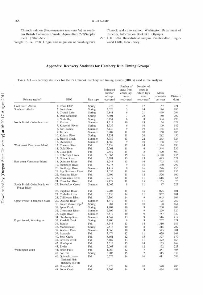
Chinook salmon (Oncorhynchus tshawytscha) in south-
ern British Columbia, Canada. Aquaculture 272(Supple-
ment 1):S161–S171.
Wright, S. G. 1968. Origin and migration of Washington’s
Chinook and coho salmon. Washington Department of
Fisheries, Information Booklet 1, Olympia.
Zar, J. H. 1984. Biostatistical analysis. Prentice-Hall, Engle-
wood Cliffs, New Jersey.
Appendix: Recovery Statistics for Hatchery Run Timing Groups
TABLE A.1.—Recovery statistics for the 77 Chinook hatchery run timing groups (HRGs) used in the analysis.
Release regiona HRG Run type
Estimatednumberof tags
recovered
Number ofareas fromwhich tags
wererecovered
Number ofyears in
which tagswere
recoveredb
Meanrecoveriesper year
Distance(km)
Cook Inlet, Alaska 1. Cook Inletc Spring 976 9 17 57 221Southeast Alaska 2. Snettisham Spring 2,020 3 14 144 186
3. Crystal Lake Spring 9,841 6 21 469 2944. Deer Mountain Spring 3,301 7 22 150 2025. Neets Bay Spring 3,154 6 8 394 196
North British Columbia coast 6. Masset Summer 1,214 10 19 64 3247. Kincolith River Spring 1,737 6 16 109 1428. Fort Babine Summer 3,130 9 19 165 1369. Terrace Summer 3,207 11 20 160 185
10. Kitimat River Spring 7,331 11 26 282 45011. Snootli Creek Summer 5,787 13 22 263 32412. Oweekeno Summer 1,380 9 10 138 353
West coast Vancouver Island 13. Conuma River Fall 15,738 12 14 1,124 29014. Gold River Fall 2,061 11 6 344 33615. Clayoquot Fall 2,452 11 5 490 56016. Robertson Creek Fall 50,365 15 16 3,148 43517. Nitinat River Fall 5,781 13 13 445 527
East coast Vancouver Island 18. Quinsam River Fall 11,248 13 16 703 45919. Puntledge River Fall 5,275 9 16 330 29720. Puntledge River Summer 4,417 8 16 276 15521. Big Qualicum River Fall 14,055 11 16 878 15322. Nanaimo River Fall 6,906 11 12 576 10023. Chemainus River Fall 17,777 11 11 1,616 6524. Cowichan River Fall 17,477 11 15 1,165 75
South British Columbia–lowerFraser River
25. Tenderfoot Creek Summer 1,065 8 11 97 227
26. Capilano River Fall 17,204 11 16 1,075 10127. Chehalis River Fall 10,250 14 11 932 10128. Chilliwack River Fall 9,390 14 9 1,043 104
Upper Fraser–Thompson rivers 29. Quesnel River Summer 1,379 11 11 125 26930. Fraser above Hoped Spring 984 12 10 98 16431. Spius Creek Spring 1,804 10 9 200 10932. Clearwater River Summer 2,509 11 9 279 32033. Eagle River Summer 6,812 10 9 757 32234. Shushwap River Summer 4,647 13 9 516 417
Puget Sound, Washington 35. Kendall Creek Spring 2,400 9 9 267 22136. Samish Fall 18,345 13 14 1,310 18637. Marblemount Spring 2,518 10 8 315 20238. Wallace River Summer 4,360 10 8 545 20139. Issaquah Fall 7,474 12 11 679 16940. Soos Creek Fall 5,661 12 15 377 17941. Grovers Creek Fall 5,187 13 11 472 16342. Hoodsport Fall 2,313 15 14 165 16843. Elwha Fall 2,063 11 12 172 223
Washington coast 44. Hoko Falls Fall 1,760 12 7 251 40845. Sol Duc Spring 2,205 15 7 315 33246. Quinault Lake–
National FishHatchery (NFH)
Fall 6,575 14 16 411 589
47. Humptulips Fall 5,778 14 10 578 48548. Forks Creek Fall 4,267 14 9 474 494
168 WEITKAMP
Dow
nloa
ded
by [
Ore
gon
Stat
e U
nive
rsity
] at
16:
29 1
7 A
ugus
t 201
1
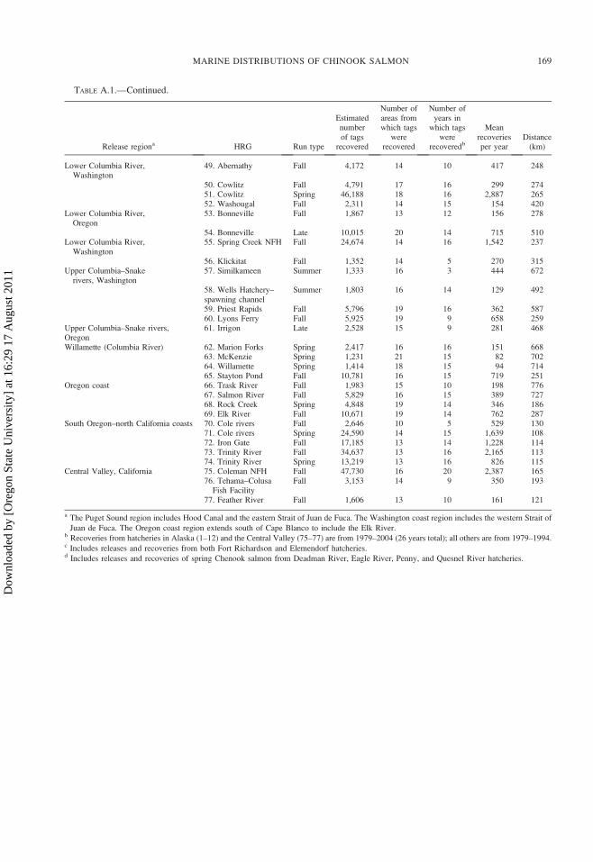
TABLE A.1.—Continued.
Release regiona HRG Run type
Estimatednumberof tags
recovered
Number ofareas fromwhich tags
wererecovered
Number ofyears in
which tagswere
recoveredb
Meanrecoveriesper year
Distance(km)
Lower Columbia River,Washington
49. Abernathy Fall 4,172 14 10 417 248
50. Cowlitz Fall 4,791 17 16 299 27451. Cowlitz Spring 46,188 18 16 2,887 26552. Washougal Fall 2,311 14 15 154 420
Lower Columbia River,Oregon
53. Bonneville Fall 1,867 13 12 156 278
54. Bonneville Late 10,015 20 14 715 510Lower Columbia River,
Washington55. Spring Creek NFH Fall 24,674 14 16 1,542 237
56. Klickitat Fall 1,352 14 5 270 315Upper Columbia–Snake
rivers, Washington57. Similkameen Summer 1,333 16 3 444 672
58. Wells Hatchery–spawning channel
Summer 1,803 16 14 129 492
59. Priest Rapids Fall 5,796 19 16 362 58760. Lyons Ferry Fall 5,925 19 9 658 259
Upper Columbia–Snake rivers,Oregon
61. Irrigon Late 2,528 15 9 281 468
Willamette (Columbia River) 62. Marion Forks Spring 2,417 16 16 151 66863. McKenzie Spring 1,231 21 15 82 70264. Willamette Spring 1,414 18 15 94 71465. Stayton Pond Fall 10,781 16 15 719 251
Oregon coast 66. Trask River Fall 1,983 15 10 198 77667. Salmon River Fall 5,829 16 15 389 72768. Rock Creek Spring 4,848 19 14 346 18669. Elk River Fall 10,671 19 14 762 287
South Oregon–north California coasts 70. Cole rivers Fall 2,646 10 5 529 13071. Cole rivers Spring 24,590 14 15 1,639 10872. Iron Gate Fall 17,185 13 14 1,228 11473. Trinity River Fall 34,637 13 16 2,165 11374. Trinity River Spring 13,219 13 16 826 115
Central Valley, California 75. Coleman NFH Fall 47,730 16 20 2,387 16576. Tehama–Colusa
Fish FacilityFall 3,153 14 9 350 193
77. Feather River Fall 1,606 13 10 161 121
a The Puget Sound region includes Hood Canal and the eastern Strait of Juan de Fuca. The Washington coast region includes the western Strait of
Juan de Fuca. The Oregon coast region extends south of Cape Blanco to include the Elk River.b Recoveries from hatcheries in Alaska (1–12) and the Central Valley (75–77) are from 1979–2004 (26 years total); all others are from 1979–1994.c Includes releases and recoveries from both Fort Richardson and Elemendorf hatcheries.d Includes releases and recoveries of spring Chenook salmon from Deadman River, Eagle River, Penny, and Quesnel River hatcheries.
MARINE DISTRIBUTIONS OF CHINOOK SALMON 169
Dow
nloa
ded
by [
Ore
gon
Stat
e U
nive
rsity
] at
16:
29 1
7 A
ugus
t 201
1
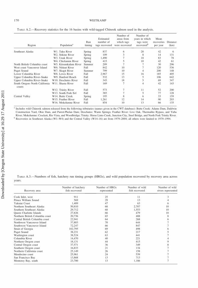
TABLE A.3.—Numbers of fish, hatchery run timing groups (HRGs), and wild population recovered by recovery area across
years.
Recovery areaNumber of hatchery
fish recoveredNumber of HRGs
representedNumber of wildfish recovered
Number of wildrivers represented
Cook Inlet, west 911 25 11 3Prince William Sound 569 29 13 4Yakutat Coast 1,489 47 63 6Northern Southeast Alaska 50,810 68 2,707 10Southern Southeast Alaska 29,712 68 1,553 10Queen Charlotte Islands 27,826 66 479 10Northern British Columbia coast 20,736 65 488 8Central British Columbia coast 22,941 64 268 6Northwest Vancouver Island 37,803 70 644 7Southwest Vancouver Island 72,247 66 847 7Strait of Georgia 102,795 69 498 6Puget Sound 38,231 62 217 5Washington coast 38,524 63 441 7Columbia River 14,470 40 221 4Northern Oregon coast 18,131 44 415 9Central Oregon coast 37,571 36 349 8Southern Oregon coast 16,833 21 134 7Northern California coast 25,149 26 158 7Mendocino coast 25,961 24 539 7San Francisco Bay 13,868 13 713 7Monterey Bay, south 23,700 13 1,186 7
TABLE A.2.—Recovery statistics for the 16 basins with wild-tagged Chinook salmon used in the analysis.
Region PopulationaRun
timing
Estimatednumber of
tags recovered
Number ofareas fromwhich tags
were recovered
Number ofyears in which
tags wererecoveredb
Meanrecoveriesper year
Distance(km)
Southeast Alaska W1. Taku River Spring 837 6 20 42 6W2. Stikine River Spring 109 3 8 14 131W3. Unuk River Spring 1,490 7 18 83 78W4. Chickamin River Spring 415 5 10 42 61
North British Columbia coast W5. Kitsumkalum River Summer 209 7 7 30 206West coast Vancouver Island W6. Nitinat River Fall 842 10 7 120 536Puget Sound W7. Skagit River Summer 799 10 4 200 148Lower Columbia River W8. Lewis River Fall 2,967 15 16 185 405Upper Columbia River–Snake W9. Hanford Reach Fall 532 13 5 106 642Upper Columbia River–Snake W10. Deschutes River Fall 345 18 5 69 347South Oregon–North California
coastsW11. Shasta River Fall 169 7 4 42 143
W12. Trinity River Fall 573 7 11 52 200W13. South Fork Eel Fall 385 7 5 77 128
Central Valley W14. Butte Creek Spring 195 8 6 33 159W15. Feather River Fall 1,261 12 14 90 203W16. Mokelumne River Fall 854 10 13 66 135
a Includes wild Chinook salmon released from the following tributaries (names given in the CWT database): Butte Creek: Adams Dam, Daldwin
Construction Yard, Okie Dam, and Parrot-Phelan Dam; Deschutes: Warm Springs; Feather River: Live Oak, Thermalito Bypass, and Yuba
River; Mokelumne: Crockett, Rio Vista, and Woodbridge; Trinity: Horse Linto Creek, Junction City, Steel Bridge, and North Fork Trinity River.b Recoveries in Southeast Alaska (W1–W4) and the Central Valley (W14–16) are from 1979–2004; all others were limited to 1979–1994.
170 WEITKAMP
Dow
nloa
ded
by [
Ore
gon
Stat
e U
nive
rsity
] at
16:
29 1
7 A
ugus
t 201
1