margin and sensitivity methods for security analysis … · margin and sensitivity methods for...
TRANSCRIPT

MARGIN AND SENSITIVITY METHODS
FOR
SECURITY ANALYSIS
OF
ELECTRIC POWER SYSTEMS
by
Scott Greene
A dissertation submitted in partial fulfillment
of the requirements for the degree of
Doctor of Philosophy
(Electrical Engineering)
University of Wisconsin – Madison
1998
Supervised by Ian Dobson
Department of Electrical and Computer Engineering
University of Wisconsin – Madison
1415 Engineering Drive, Madison WI 53706 USA

c© Copyright by Scott Greene 1998
All Rights Reserved

Abstract
Reliable operation of large scale electric power networks requires that system voltages
and currents stay within design limits. Operation beyond those limits can lead to
equipment failures and blackouts. Security margins measure the amount by which
system loads or power transfers can change before a security violation, such as an
overloaded transmission line, is encountered.
This thesis shows how to efficiently compute security margins defined by limiting
events and instabilities, and the sensitivity of those margins with respect to assump-
tions, system parameters, operating policy, and transactions. Security margins to
voltage collapse blackouts, oscillatory instability, generator limits, voltage constraints
and line overloads are considered. The usefulness of computing the sensitivities of
these margins with respect to interarea transfers, loading parameters, generator dis-
patch, transmission line parameters, and VAR support is established for networks as
large as 1500 buses.
The sensitivity formulas presented apply to a range of power system models.
Conventional sensitivity formulas such as line distribution factors, outage distribution
factors, participation factors and penalty factors are shown to be special cases of the
general sensitivity formulas derived in this thesis. The sensitivity formulas readily
accommodate sparse matrix techniques.
Margin sensitivity methods are shown to work effectively for avoiding voltage
collapse blackouts caused by either saddle node bifurcation of equilibria or immediate
instability due to generator reactive power limits. Extremely fast contingency analysis
for voltage collapse can be implemented with margin sensitivity based rankings.
Interarea transfer can be limited by voltage limits, line limits, or voltage stability.
The sensitivity formulas presented in this thesis apply to security margins defined
by any limit criteria. A method to compute transfer margins by directly locating
intermediate events reduces the total number of loadflow iterations required by each
margin computation and provides sensitivity information at minimal additional cost.
Estimates of the effect of simultaneous transfers on the transfer margins agree well
with the exact computations for a network model derived from a portion of the U.S
grid. The accuracy of the estimates over a useful range of conditions and the ease of
obtaining the estimates suggest that the sensitivity computations will be of practical
value.
i

This thesis is dedicated to the caring educatorsof my youth.

Acknowledgments
I cherish the friendships that accompanied my studies here at the University of Wis-
consin. I thank my wife, my children, my parents, and my sister for their enduring
love and support.
I appreciate the guidance, dedication, and exemplary academic standards of my
advisor, Professor Ian Dobson. I am also indebted to Professor Fernando Alvarado
for his counsel, insight, and encouragement. I thank Professor Chris DeMarco for
numerous enlightening discussions and his willingness to entertain my aberrant ques-
tions. I have enjoyed the instruction and advisement of Professor Bill Long since
before starting graduate school, and I am thankful for his participation on my thesis
committee. I am grateful to Joel Robbin, Professor of Mathematics, for many hours
of tutoring and for giving me an entirely different perspective on engineering.
Professor Claudio Canizares of the University of Waterloo developed software that
started this research and I thank him for his support and friendship.
I thank Dr. Arthur Ekwue and the National Grid Company plc of the United
Kingdom for their interest in our work and for providing the test data and motivation
for the research presented in Chapter 7.
I thank the Grainger Foundation for their generosity and support of the power
engineering program at the University of Wisconsin.
Funding in part from National Science Foundation PYI grant ECS-9157192 and
from the Electric Power Research Institute under contracts RP8010-30, RP8050-03,
WO8050-03 is gratefully acknowledged. Funding in part from the Empire State Elec-
tric Energy Research Corporation and New York State Electric and Gas under ES-
EERCO project EP 95-11 is gratefully acknowledged. The support of the Power
System Engineering Research Center (PSerc) is gratefully acknowledged.
iii

iv
Contents
Abstract i
Acknowledgments iii
1 Introduction 1
1.1 Motivation . . . . . . . . . . . . . . . . . . . . . . . . . . . . . . . . . 1
1.2 Margins and sensitivity . . . . . . . . . . . . . . . . . . . . . . . . . . 2
1.3 Literature review . . . . . . . . . . . . . . . . . . . . . . . . . . . . . 3
1.4 Summary . . . . . . . . . . . . . . . . . . . . . . . . . . . . . . . . . 4
2 Assumptions 7
2.1 Power system operation . . . . . . . . . . . . . . . . . . . . . . . . . 7
2.2 Assumptions . . . . . . . . . . . . . . . . . . . . . . . . . . . . . . . . 10
3 Margin Computations 17
3.1 Previous work . . . . . . . . . . . . . . . . . . . . . . . . . . . . . . . 17
3.2 Anatomy of margin computations . . . . . . . . . . . . . . . . . . . . 18
3.2.1 Description of margin computation program . . . . . . . . . . 25
3.3 Summary . . . . . . . . . . . . . . . . . . . . . . . . . . . . . . . . . 27
4 Sensitivity Computations 29
4.1 Methods of sensitivity analysis . . . . . . . . . . . . . . . . . . . . . . 29
4.2 Sensitivity formulas . . . . . . . . . . . . . . . . . . . . . . . . . . . . 35
4.2.1 Derivation . . . . . . . . . . . . . . . . . . . . . . . . . . . . . 35
4.2.2 Normal vector to the event boundary in parameter space . . . 38
4.2.3 General derivation . . . . . . . . . . . . . . . . . . . . . . . . 39
4.2.4 Fold bifurcation . . . . . . . . . . . . . . . . . . . . . . . . . . 44
4.2.5 Hopf bifurcation and eigenvalue sensitivity . . . . . . . . . . . 45
4.3 Traditional sensitivity . . . . . . . . . . . . . . . . . . . . . . . . . . 47
4.4 Penalty factors, β coefficients, and normal vectors . . . . . . . . . . . 53
4.5 Example: line overload . . . . . . . . . . . . . . . . . . . . . . . . . . 55
5 Voltage Collapse 59
5.1 Introduction . . . . . . . . . . . . . . . . . . . . . . . . . . . . . . . . 59
5.2 Theoretical background and assumptions . . . . . . . . . . . . . . . . 62
v
5.3 Informal derivation . . . . . . . . . . . . . . . . . . . . . . . . . . . . 63
5.4 Application to test system . . . . . . . . . . . . . . . . . . . . . . . . 64
5.4.1 Emergency load shedding . . . . . . . . . . . . . . . . . . . . 65
5.4.2 Direction of load increase . . . . . . . . . . . . . . . . . . . . . 67
5.4.3 Reactive power support . . . . . . . . . . . . . . . . . . . . . 67
5.4.4 Area interchange . . . . . . . . . . . . . . . . . . . . . . . . . 67
5.4.5 Load model . . . . . . . . . . . . . . . . . . . . . . . . . . . . 71
5.4.6 Line susceptance . . . . . . . . . . . . . . . . . . . . . . . . . 71
5.4.7 Generator dispatch . . . . . . . . . . . . . . . . . . . . . . . . 71
5.5 Discussion . . . . . . . . . . . . . . . . . . . . . . . . . . . . . . . . . 74
5.6 Conclusions . . . . . . . . . . . . . . . . . . . . . . . . . . . . . . . . 76
5.7 Appendices . . . . . . . . . . . . . . . . . . . . . . . . . . . . . . . . 77
5.7.A Derivation of sensitivity formulas . . . . . . . . . . . . . . . . . 77
5.7.B Construction of Ψ. . . . . . . . . . . . . . . . . . . . . . . . . . 78
5.7.C Locally closest fold bifurcation. . . . . . . . . . . . . . . . . . . 79
6 Contingency Analysis for Voltage Collapse 81
6.1 Introduction . . . . . . . . . . . . . . . . . . . . . . . . . . . . . . . . 81
6.2 Previous work . . . . . . . . . . . . . . . . . . . . . . . . . . . . . . . 83
6.3 Results . . . . . . . . . . . . . . . . . . . . . . . . . . . . . . . . . . . 85
6.3.1 1390 bus system . . . . . . . . . . . . . . . . . . . . . . . . . . 85
6.3.2 All single contingencies of the 118 bus system . . . . . . . . . 86
6.3.3 Multiple contingencies of 118 bus system . . . . . . . . . . . . 88
6.4 Discussion . . . . . . . . . . . . . . . . . . . . . . . . . . . . . . . . . 90
6.5 Computations . . . . . . . . . . . . . . . . . . . . . . . . . . . . . . . 91
6.5.1 Linear estimate formula . . . . . . . . . . . . . . . . . . . . . 92
6.5.2 Quadratic estimate formula . . . . . . . . . . . . . . . . . . . 93
6.5.3 Computational efficiency . . . . . . . . . . . . . . . . . . . . . 94
6.6 Conclusion . . . . . . . . . . . . . . . . . . . . . . . . . . . . . . . . . 95
7 Margin Sensitivity Applications 97
7.1 Introduction . . . . . . . . . . . . . . . . . . . . . . . . . . . . . . . . 98
7.2 Nominal voltage collapse margin . . . . . . . . . . . . . . . . . . . . . 98
7.3 Loading margin sensitivity . . . . . . . . . . . . . . . . . . . . . . . . 103
7.4 Contingency ranking for voltage collapse . . . . . . . . . . . . . . . . 108
7.5 Voltage collapse due to VAR limits . . . . . . . . . . . . . . . . . . . 114
7.6 Ranking for voltage collapse due to VAR limits . . . . . . . . . . . . 117
7.7 Large deviation contingency analysis . . . . . . . . . . . . . . . . . . 123
7.8 Conclusions . . . . . . . . . . . . . . . . . . . . . . . . . . . . . . . . 125
vi

8 Sensitivity of Transfer Capability Margins 129
8.1 Introduction . . . . . . . . . . . . . . . . . . . . . . . . . . . . . . . . 129
8.2 Overview of transfer capability determination . . . . . . . . . . . . . 130
8.3 Sensitivity . . . . . . . . . . . . . . . . . . . . . . . . . . . . . . . . . 134
8.3.1 Assumptions . . . . . . . . . . . . . . . . . . . . . . . . . . . . 134
8.3.2 Sensitivity formulas . . . . . . . . . . . . . . . . . . . . . . . . 135
8.4 Example . . . . . . . . . . . . . . . . . . . . . . . . . . . . . . . . . . 136
8.4.1 40 bus system . . . . . . . . . . . . . . . . . . . . . . . . . . . 137
8.4.2 1500 bus system . . . . . . . . . . . . . . . . . . . . . . . . . . 142
8.4.3 Sensitivity of the transfer capability to transactions . . . . . . 144
8.4.4 Computational efficiency . . . . . . . . . . . . . . . . . . . . . 147
8.5 Discussion . . . . . . . . . . . . . . . . . . . . . . . . . . . . . . . . . 148
8.6 Conclusions and Future Work . . . . . . . . . . . . . . . . . . . . . . 148
9 Interarea Oscillations 149
9.1 Introduction . . . . . . . . . . . . . . . . . . . . . . . . . . . . . . . . 149
9.2 Assumptions and model . . . . . . . . . . . . . . . . . . . . . . . . . 150
9.3 Motivation . . . . . . . . . . . . . . . . . . . . . . . . . . . . . . . . . 154
9.4 Computations . . . . . . . . . . . . . . . . . . . . . . . . . . . . . . . 155
9.5 Results . . . . . . . . . . . . . . . . . . . . . . . . . . . . . . . . . . . 158
9.6 Discussion and conclusions . . . . . . . . . . . . . . . . . . . . . . . . 168
9.7 Appendix . . . . . . . . . . . . . . . . . . . . . . . . . . . . . . . . . 170
10 Conclusions and Future Research 175
10.1 Conclusions . . . . . . . . . . . . . . . . . . . . . . . . . . . . . . . . 175
10.2 Future work . . . . . . . . . . . . . . . . . . . . . . . . . . . . . . . . 177
Bibliography 181
vii

viii

List of Figures
1 Phase portraits and equilibrium trajectory as parameter changes and
state remains within each basin of attraction . . . . . . . . . . . . . . 12
2 Phase portraits and equilibrium trajectory as parameter changes and
state does not remain within each basin of attraction . . . . . . . . . 13
3 Equilibria trajectories for different values of the parameter p . . . . . 30
4 Nominal trajectory and boundary as function of the parameter p . . . 32
5 Nominal trajectory and estimated boundary . . . . . . . . . . . . . . 34
6 Nose curves as parameter p varies . . . . . . . . . . . . . . . . . . . . 61
7 Loading margin as parameter p varies . . . . . . . . . . . . . . . . . . 61
8 Effect of load shedding on voltage collapse margin . . . . . . . . . . . 66
9 Effect of assumed loading direction on voltage collapse margin . . . . 68
10 Effect of shunt capacitance on voltage collapse margin . . . . . . . . . 69
11 Effect of import into critical area on voltage collapse margin . . . . . 70
12 Effect of composition of load model on voltage collapse margin . . . . 72
13 Effect of susceptance on voltage collapse margin . . . . . . . . . . . . 73
14 Effect of generator dispatch on voltage collapse margin . . . . . . . . 75
15 Nominal and contingency nose curves . . . . . . . . . . . . . . . . . . 82
16 Effect of load increase at Indian Queens on the loading margin to
voltage collapse . . . . . . . . . . . . . . . . . . . . . . . . . . . . . . 109
17 Effect of load decrease at Indian Queens on the loading margin to
voltage collapse . . . . . . . . . . . . . . . . . . . . . . . . . . . . . . 110
18 Effect of load decrease at Indian Queens on the loading margin to
voltage collapse and critical VAR limit . . . . . . . . . . . . . . . . . 111
19 Effect of variation in VAR limits at Exeter on the loading margin to
voltage collapse . . . . . . . . . . . . . . . . . . . . . . . . . . . . . . 112
20 Critical bus voltage versus transfer to Area 3 . . . . . . . . . . . . . . 137
21 Effect of simultaneous transfer on transfer capability limited by low
voltage . . . . . . . . . . . . . . . . . . . . . . . . . . . . . . . . . . . 138
22 Effect of simultaneous transfer on transfer capability limited by voltage
collapse . . . . . . . . . . . . . . . . . . . . . . . . . . . . . . . . . . 139
23 Effect of generator dispatch on transfer capability limited by low voltage140
ix

24 Effect of load variation at a critical bus on transfer capability limited
by low voltage . . . . . . . . . . . . . . . . . . . . . . . . . . . . . . . 141
25 Effect of reactive power support on transfer capability limited by low
voltage . . . . . . . . . . . . . . . . . . . . . . . . . . . . . . . . . . . 142
26 Effect of simultaneous transfer on margin to first flow limit . . . . . . 145
27 Effect of simultaneous transfer on margin to voltage limit . . . . . . . 146
28 One line diagram of 3 bus test system . . . . . . . . . . . . . . . . . . 158
29 Effect of generation dispatch on Hopf margin . . . . . . . . . . . . . . 159
30 Effect of generation dispatch on Hopf margin, extended variation . . . 160
31 Trajectory of critical eigenvalues as generator dispatch is varied for
generator terminal voltage of 1.00 p.u. . . . . . . . . . . . . . . . . . 161
32 Trajectory of critical eigenvalues as generator dispatch is varied for
generator terminal voltage of 1.05 p.u. . . . . . . . . . . . . . . . . . 162
33 Trajectory of critical eigenvalues as generator dispatch is varied for
generator terminal voltage of 1.10 p.u. . . . . . . . . . . . . . . . . . 163
34 One line diagram of 9 bus test system . . . . . . . . . . . . . . . . . . 164
35 Least damped eigenvalues at base case of 9 bus system. . . . . . . . . 165
36 Movement of least damped eigenvalues as transfer to Area 3 increases. 166
37 Movement of critical eigenvalue as transfer to Area 3 increases. . . . . 166
38 Damping of critical mode versus linear estimate as function of transfer
to Area 3 in 9 bus system. . . . . . . . . . . . . . . . . . . . . . . . . 167
39 Linear estimate and actual margin to oscillations as function of export
to Area 2 in 9 bus system. . . . . . . . . . . . . . . . . . . . . . . . . 167
40 Effect of interarea exchange on damping of 37 bus system . . . . . . . 169
x

List of Tables
1 Estimated loading margins for all 500kV line outages in a critical area
of the 1390 bus system. . . . . . . . . . . . . . . . . . . . . . . . . . . 87
2 Estimated loading margins for the 25 worst outages of the 118 bus
system. . . . . . . . . . . . . . . . . . . . . . . . . . . . . . . . . . . . 89
3 Transformer data . . . . . . . . . . . . . . . . . . . . . . . . . . . . . 99
4 Branch data . . . . . . . . . . . . . . . . . . . . . . . . . . . . . . . . 100
5 Nominal stable operating point . . . . . . . . . . . . . . . . . . . . . 101
6 Reactive power limits . . . . . . . . . . . . . . . . . . . . . . . . . . . 102
7 Direction of load increase . . . . . . . . . . . . . . . . . . . . . . . . . 102
8 Nominal point of collapse . . . . . . . . . . . . . . . . . . . . . . . . . 104
9 Left eigenvector corresponding to the zero eigenvalue of the system
Jacobian at the nominal point of collapse . . . . . . . . . . . . . . . . 105
10 Estimated and actual changes in the loading margin to fold bifurcation
resulting from severe non-radial line outages . . . . . . . . . . . . . . 114
11 Estimated and actual changes in the loading margin to fold bifurcation
resulting from radial line outages . . . . . . . . . . . . . . . . . . . . 115
12 Estimated and actual changes in the loading margin to fold bifurcation
resulting from less severe non-radial line outages . . . . . . . . . . . . 116
13 Estimated and actual changes in the loading margin to voltage collapse
resulting from severe non-radial line outages . . . . . . . . . . . . . . 117
14 Estimated and actual changes in the loading margin to voltage collapse
resulting from radial line outages . . . . . . . . . . . . . . . . . . . . 118
15 Estimated and actual changes in the loading margin to voltage collapse
resulting from less severe non-radial line outages . . . . . . . . . . . . 119
16 The loading margins to fold bifurcation and voltage collapse for all line
outages causing an immediate instability prior to fold bifurcation . . 120
17 Comparison of the normal vectors to the parameter set corresponding
to fold bifurcation (W) and immediate instability (N) . . . . . . . . . 122
18 Comparison of linear estimated changes in the loading margin to volt-
age collapse resulting from severe non-radial line outages . . . . . . . 123
19 Comparison of linear estimated changes in the loading margin to volt-
age collapse resulting from less severe non-radial line outages . . . . . 124
xi
20 Comparison of linear, quadratic, and large deviation estimates for
changes in the loading margin to voltage collapse resulting from se-
vere non-radial line outages . . . . . . . . . . . . . . . . . . . . . . . 126
21 Comparison of linear, quadratic, and large deviation estimates for
changes in the loading margin to voltage collapse resulting from less
severe non-radial line outages . . . . . . . . . . . . . . . . . . . . . . 127
22 Area exports at base case, nominal transfer limit, and contingency
transfer limit . . . . . . . . . . . . . . . . . . . . . . . . . . . . . . . 143
23 Sensitivities of the transfer margin with respect to area exports . . . 144
xii
Chapter 1
Introduction
This thesis concerns the stability and security of large electric power systems with
an emphasis on static or longer term stability. One contribution of this thesis is the
establishment of a coherent, consistent, and general framework for margin and sen-
sitivity analysis applicable to a variety of security criteria. This thesis shows how
to efficiently compute the security margins defined by limiting events and instabili-
ties, and the sensitivity of those margins with respect to any model parameter. This
chapter introduces the important concepts and includes an explanation of the most
relevant previous work and a brief summary of the thesis. Chapter 2 states assump-
tions defining admissible power system models. Chapters 3 and 4 detail computational
methods for computing margins and their sensitivities. Chapters 5, 6, and 7 describe
applications regarding voltage collapse. Chapter 8 describes applications regarding
transfer capability. Chapter 9 describes applications regarding oscillatory instabili-
ties. Chapter 10 contains a summary of the thesis and outlines possible avenues for
future work.
1.1 Motivation
Power systems are affected by events that depend upon the state (voltages and cur-
rents) of the power system. The state of the power system is influenced by both
controllable and uncontrollable factors.
For instance, as loads increase, the system generation must increase to keep power
balance and maintain reserve and security margins. Often, at high load levels, gen-
erators reach real and reactive power limitations and the flows on lines exceed limits.
Any of these events can initiate a change in the operation of the power system. The
change in operation is reflected by a change in the equations that model the power
system, or the nature of the solutions that the equations yield. Fundamental questions
of system security, and the questions addressed by this thesis, are:
“How close is the system to the next event?”
“Will the system remain stable after the next event?”
“How can the margin to the next event be increased?”
1

2 CHAPTER 1. INTRODUCTION
1.2 Margins and sensitivity
Some parameters can be set or controlled and others, like loads, are mostly uncon-
trolled. The uncontrolled parameters can vary with time and affect the behavior of
the power system. The difference between the parameter values corresponding to an
event and the current or nominal parameters defines the margin to the event. For
instance, when an increase in loading causes the flow on a line to exceed its rating,
the distance to the line overload can be measured by a suitable norm of the vector
difference in loads, a loading margin. Depending on the application, security margins
can be measured in parameter space with respect to load levels, load model param-
eters, import levels, temperature, or time. When the security margin measures the
distance to an event that causes the system to become unstable, it is called a stability
margin.
In some instances, it may be practical to measure the security margin with a state
variable or a function of state. For example, the amount of additional real power flow
on a line that would cause overload is an easily understood measure of closeness to
overload of that line. Examples of margins measured in state space are increments in
line flows, generator VAR outputs, and voltage levels.
The system equilibrium, and thus margins to events, is affected by both control-
lable and uncontrollable parameters. The sensitivity of margins with respect to un-
controllable parameters quantifies the effects of different assumptions, forecasts, and
measured data. System operation also requires knowledge of how the controllable
parameters can be adjusted to keep the system secure as the uncontrollable parame-
ters change. One way of quantifying the effectiveness of controls is by computing the
sensitivity of the security margin with respect to the control parameter.
Consider the case of a line approaching overload. By computing the sensitivity of
the line flow with respect to different loading patterns, one can estimate the worst
case loading pattern — the one that increases the line flow most rapidly. The loading
margin for this load pattern can then be computed by solving for a continuation of
equilibria as the loading level is gradually increased. 1
Once the loading level at which the line reaches overload is located and hence
the loading margin found, the sensitivity of the loading margin with respect to any
parameters can be calculated. For example, computing the sensitivity of the margin
with respect to the area export set points can be used to assess the possibility of
avoiding the overload by changing the export schedules.
1The continuation neglects the transients and dynamics of the power system. However, the locusof equilibria approximates the trajectory of the system state for sufficiently stable dynamics andslowly varying load level.
1.3. LITERATURE REVIEW 3
This thesis describes how to compute margins to several events, compute the sen-
sitivity of the margins with respect to any parameters, and investigates applications
for the margin and sensitivity computations.
1.3 Literature review
This section contains a brief review of literature helpful for understanding the material
presented in this thesis. The references in this section are relevant to the thesis as a
whole and to the material presented in Chapters 2,3, and 4 in particular.
Several textbooks outside the field of power engineering were particularly useful
for this thesis. The derivations and computational methods presented in Chapters 3
and 4 require an understanding of multivariable calculus. The first two chapters of
[Spivak] and the first chapter of [GP] are recommended. [GV] is an excellent reference
for matrix computations and [HJ] for matrix theory. [BN] is an accessible and clear
reference for differential equations. [GH] is a popular reference for bifurcations but is
not as accessible to the engineer as [Seydel]. [Seydel] is a valuable reference concerning
computations and bifurcations and is most frequently cited in power systems papers
concerning voltage collapse computations. [GZ] presents an exceptional explanation
of the path following, or continuation methods, that form the backbone of the methods
in this report.
The fundamentals of modeling electric power systems are covered in [Bergen],
[WW], [Kundur], and [SauPai]. [Bergen] is the most understandable. [Kundur] is
the most comprehensive and contains a good analysis of generator reactive power
limits. [WW] best describes utility interconnections and economics. [SauPai] has
the clearest explanation of small signal stability, the effects of load models, and Hopf
bifurcations. [Heydt] is the most complete text describing power system computations
but is becoming outdated.
Supplemental to these texts, two survey papers provide good explanation of static
[Sto74] and dynamic [Sto79] power system models and computations. [PPTT], [SM79],
and [DT68] are landmark papers concerning sensitivity, optimization, and computa-
tion in power systems.
Van Cutsem [VC91, VC95, VC293, VC96] has forwarded an approach to steady
state stability analysis influential to this thesis. Specifically, Van Cutsem embraces
the use of loading margins that are path dependent and account for discrete events,
utilizes sensitivities and promotes the use of path following methods as static simula-
tion tools. Van Cutsem also provided the useful interpretation of margin sensitivities
in terms of the Lagrange multipliers of an optimization problem. The new text [VCK]
contains the aggregate of Van Cutsem’s work and a complete description of voltage

4 CHAPTER 1. INTRODUCTION
stability theory and application.
[WF93] and the discussion by Wu, Fischl, and Nwankpa in [GDA97] has also
influenced this thesis, suggesting the use of continuation and sensitivity methods to
assess interarea transfer margins, proposing the use of first and second order Taylor
series estimates for contingency analysis [GDA98], and presenting the transfer margin
computation as an optimization problem.
Chapters 5, 6, and 7 concern voltage collapse in electric power systems. [DCL,
Davos, IEEE1] cover the full breadth of case studies, research and opinions on voltage
collapse. [GDA97] is a concise version of Chapter 5 and computes Taylor series
estimates of the bifurcation set for a practical power system model accounting for
generator reactive power limits. Chapter 9 concerns oscillatory instability in power
systems. [IEEE1] contains a broad range of ideas and experiences concerning interarea
oscillations in power systems.
The research contained in this thesis builds upon earlier work conducted at the
University of Wisconsin. [AJ89] presents a direct method to locate a saddle node
bifurcation point of a power system model and [CA93] compares a continuation
method with a direct method. A more tutorial and detailed presentation is found
in [CanPhD] and [CA91] incorporating models for HVDC systems. Several papers
[Dob93, DL93, ADH94] concern locating the closest saddle node bifurcation to an
operating point or optimizing the distance in parameter space to a bifurcation point
[DL192, Can98]. [DL192] first demonstrates computation of the voltage collapse load-
ing margin sensitivity from the components of the normal vector to the bifurcation set
in parameter space. Derivation of the normal vector to the saddle-node bifurcation
set in parameter space is presented in [Dob92]. Analysis of the immediate instability
precipitated by a generator reactive power limit is contained in [DL292]. [DAD92]
concerns the sensitivity of Hopf bifurcations in power systems.
1.4 Summary
This thesis demonstrates that the sensitivity of the security margin to an event can
be computed with respect to any system parameter, and that the sensitivities are
practical and useful for control, computation, and contingency analysis.
This thesis considers security margins to events defined by voltage collapse and fold
bifurcations, oscillatory instability and Hopf bifurcations, immediate instability due
to generator reactive power limits, voltage limits and line flow limits. The usefulness
of computing the sensitivities of these margins with respect to interarea transfers, load
change and load model parameters, generator dispatch, transmission line parameters
and line compensation, and VAR support is established for systems as large as 1500

1.4. SUMMARY 5
buses.
Chapter 2 motivates and states the basic steady state modeling assumptions used
in this thesis. Chapter 3 presents a thorough explanation of path following methods
for power system security margin computations and improves and extends earlier
work specific to voltage collapse. Established continuation methods for computing
security margins can be improved to directly locate intermediate events of practical
interest. The intermediate events are often points at which the equations that model
the system change. Correct computation of security margins requires that these
intermediate events be accounted for.
Chapter 4 describes how the sensitivity of security margins with respect to system
parameters can be computed and used to estimate an operational boundary in param-
eter space. Sensitivity based estimates can be used to quickly assess the quantitative
effectiveness of various control actions to maintain a sufficient security margin. The
estimates are also useful in determining the importance of uncertainties in data or
model assumptions. The evaluation of the estimates for large power system models
is very efficient. Chapter 4 contains a rigorous and general derivation. It is also
shown that the general sensitivity formulas can, in special cases, be reduced to yield
established sensitivity formulas such as line distribution factors, outage distribution
factors, participation factors and penalty factors.
Chapter 5 demonstrates the practical use of the sensitivity computations for a
range of system parameters on a voltage collapse of the IEEE 118 bus system. The
closeness of the estimates over a useful range of parameter variations and the ease
of obtaining the linear estimate suggest that the sensitivity computations will be of
practical value in avoiding voltage collapse. Chapter 5 contains a rigorous derivation
of the linear and quadratic sensitivity of the loading margin to voltage collapse with
respect to arbitrary parameters and includes material published in [GDA97] and noted
in [VCK].
Chapter 6 extends the work of Chapter 5 to contingency analysis. Chapter 6 shows
that effective contingency ranking for voltage collapse can be obtained by computing
the loading margin sensitivities with respect to each line outage. This approach
can take into account some of the effects of reactive power limits and easily handles
multiple contingencies. The results show that the linear estimates are extremely fast
and provide acceptable contingency ranking. Chapter 6 includes material published
in [GDA98].
Chapter 7 tests the methods of Chapters 5 and 6 on a 40 bus model of the National
Grid Company of the United Kingdom and introduces several new applications. It is
shown that the methods applied to voltage collapse precipitated by fold bifurcation
can be successfully adapted to voltage collapse precipitated by a generator VAR
6 CHAPTER 1. INTRODUCTION
limit. In addition, computation of the sensitivity of the loading margin to voltage
collapse with respect to changes in generator VAR limits is demonstrated. Finally,
the contingency computations of Chapter 6 that model a line outage as a change in
the sparse bus admittance matrix are recomputed instead using changes in the dense
bus impedance matrix (analogous to large deviation outage distribution factors). The
results suggest that this approach is of questionable benefit.
Chapter 8 demonstrates how margin and sensitivity computations can be used to
determine transfer capability margins. The methods are tested on a 1500 bus power
system model. The sensitivity of the transfer margin with respect to area exports is
used to obtain estimates of the effect of simultaneous transfers on transfers limited
by both line flow limits and voltage limits. The results indicate that the methods
should be useful in determining available transfer capabilities.
Chapter 9 describes applications concerning oscillatory instability margins and
eigenvalue sensitivity. Chapter 9 demonstrates the computation of the transfer mar-
gins to oscillatory instability and the sensitivity of these margins with respect to
import set points. If the difficulties attributable to very large system models can be
addressed, the computation would be of practical value in assessing interarea transfer
policies in a deregulated environment.
The conclusions of this thesis are discussed in Chapter 10 together with suggestions
for future work.
Chapter 2
Assumptions
This chapter contains the basic assumptions that provide the foundation for the meth-
ods presented in this report. The mathematical model of a power system presented in
this chapter is general and provides the basis for the computational methods presented
in later chapters for computing security margins and sensitivities of margins.
A useful model accurately recreates some phenomena of the actual system and
specifies which phenomena are ignored and the conditions for which the model is
valid. The simplifying assumptions used to derive a model determine the phenomena
that will be accurately portrayed and those that will be missed.
It is poor engineering practice to assume that an actual system will behave ideally.
However, it is worse practice to operate an actual system in conditions in which even
an ideal system could not properly function. The purpose of steady state stability
analysis in power systems is to identify the operational limits of an ideal system.
One objective of this chapter is to show how to locate the points at which the power
system could not effectively operate subject even to small disturbances. Experience
and judgment can be employed to determine a sufficient safety margin for the actual
system. In the next section we describe the characteristics of the power system to be
included in our model, and distinguish those that will be neglected.
2.1 Power system operation
The methods and assumptions of this thesis are motivated here by a brief description
of power system operation. Power systems interconnect millions of electrical and
mechanical devices. The variety of phenomena exhibited by an actual power system
is immense. The following description includes only the relevant characteristics of
which only a subset will be retained by our model.
One can view the power system as an enormous nonlinear electric circuit1. The
1Modeling a power system as an electric circuit may seem obvious to electrical engineers. However,models of power systems that greatly simplify or ignore the underlying circuit are common anduseful for economic analysis. For modeling gross behavior like emissions or expenditures on a dailyor monthly time scale, circuit descriptions of the system are not useful.
7
8 CHAPTER 2. ASSUMPTIONS
model should retain the fundamental characteristics of electric circuits and the de-
pendence of state variables (voltages and currents) on circuit parameters.
Many power system phenomena are initiated by the aggregate effect of changing
loads. The model should have the ability to partially account for the response of
interconnected generators to fluctuating demands. As loads increase the rotational
speed and hence frequency of individual generators decreases. A control system using
frequency as a feedback increases the mechanical input to the generators which in turn
results in increased electrical output and restoration of frequency. Another control
system implements a dispatch among generators so that increased output is provided
by those generators at which it is most economical to do so and so that interchange
agreements for the transfer of power between areas and utilities are maintained.
With a cumulative increase in demand, system voltages can decline, initiating
several activities. On load tap changing transformers adjust tap positions to main-
tain load side voltages. Shunt capacitors are switched in to provide reactive power
support. Fast starting back-up generation may be brought on-line. The characteristic
of changing system equipment and structure as a function of system state is a feature
we wish to incorporate in our model.
While the demand and then generation increase, so do the flows and losses on
the transmission lines, as well as the flows and losses in the circuits and devices that
make up each generating unit.
When the flows on transmission lines increase, the temperature of the conductors
increases resulting in a loss of mechanical strength and increased sag. The increased
sag can cause a line to become dangerously close to ground increasing the possibility of
flash over and faults. A faulted line can lead to momentary or prolonged outage of the
line. Extended operation of a line beyond its thermal rating can permanently reduce
the strength of the line. Once lines become overloaded, generation is redispatched to
relieve the overloads, and in some cases the lines are interrupted to prevent permanent
damage.
Generators can be damaged by overheating and over or under voltage conditions.
Protective devices range from controls that remove the generator from the network
(severe over or under voltage), to those that limit the output of the generator by
controlling its operation. The latter include mechanical limits on the prime mover to
fix the maximum power output, and control devices that limit the voltage or current
in control circuits or generator windings to prevent overheating, shorting, and unit
failure.
The model should account for the operation of protective devices and changes in
system operation policy resulting from the condition of the system.
Every change in load or generation, switching of a device, or tap change at a

2.1. POWER SYSTEM OPERATION 9
transformer is a disturbance to the power system. Disturbances may also be caused
by random events like lightning strikes and short circuits. If the system is stable, the
controls and dynamics will behave in such a way as to move the system state toward
a new equilibrium after the disturbance. As the system becomes less stable, the rate
at which the system approaches equilibrium after every disturbance decreases. The
duration of time for which the transient effects of a disturbance dominate increases
as the stability of the system decreases. Significantly large disturbances can cause
the system state to diverge from the equilibrium or for the equilibrium to disappear.
When conditions are severe, several generators may reach operational limits and
lines may trip due to shorts caused by steady overload, in turn further compromising
the system security. The security of a system thus depends upon the accumulated
effects of slow events (gradual demand increase and generation response) and discrete
events (protective device operation), as well as the immediate effects of transients.
When the system is unstable or marginally stable, a small disturbance may prop-
agate and grow, eventually causing cascading operation of protective devices. Even
when the system is stable, large random disturbances such as lightning can propa-
gate and trip protective devices. These phenomena, although of importance to power
system operation, are not exhibited by our model.
We wish to include in our model as many of the operational parameters and
characteristics that can reasonably be controlled or forecast, and neglect those that are
beyond control or prediction. For instance, we account for the steady state evolution
of a power system due to protective device and system operation including generator
limits, but we ignore the transient effects caused by operation of the protective devices.
We account for the long term effects of generator dispatch and interarea agreements
but ignore the short time frame effects initiated by the systems that implement those
policies.
We do not account for transient behavior, protective device coordination, or in-
stantaneous limits. Hence we do not model power systems during periods when we
know that transient effects are dominant. For example, we do not model the large
disturbance response of a stable power system, or the dynamic evolution of an unsta-
ble power system. For this reason, the type of analysis emphasized in this thesis is
classified as “steady-state” or “static” as opposed to “transient” or “dynamic”.
The purpose of the next section is to specify the assumptions for a model of a
stable power system so that an unstable system can be detected from the model as a
condition at which the assumptions are violated or become contradictory.
10 CHAPTER 2. ASSUMPTIONS
2.2 Assumptions
In this section we state the primary assumptions underlying the methods presented
in this report for computing security margins and their sensitivities with respect to
parameters. Our primary assumptions are qualitative and not dependent upon spe-
cific equations for the power system. However, secondary assumptions concerning
the quantitative behavior of the power system are necessary for computation and
simulation for any particular application. In this section we state primary assump-
tions essential to motivate the following chapters. In later sections that detail specific
applications, the assumptions necessary for that application will be stated.
We assume that the dynamic behavior of the power system can be represented by
parameterized differential equations,
z = f(z, λ, u) (1)
and difference equations
uk+1 = h(z, λ, uk) (2)
where
z ∈ IRn is the vector of state variables.
λ ∈ IRm is a vector of parameters.
u is a vector of discrete states.
f is continuously differentiable with respect to z,λ and p for every u.
The differential equations (1) account for the circuit behavior and evolution of
state resulting from fluctuating demands. The difference equations (2) account for
the evolution of state due to operation of protective devices, tap changes and other
discrete events.
The distinction between variables and parameters is crucial. Parameters are ac-
tive; they are directly set or assumed. Variables are passive; they assume the values
imposed by solution of the equations. Perhaps the most important aspect of modeling
is determining or assuming what is a parameter and what is a variable. The choice
of variables and parameters can vary for each application.
Our primary assumptions are:
1. At every moment the power system has a state corresponding to a particular
exponentially stable equilibrium solution of equation (1). This state is referred
to as the equilibrium state.
2.2. ASSUMPTIONS 11
2. The operation of state dependent devices can be considered to be dependent
upon the equilibrium state.
3. The system state remains in the basin of attraction of the equilibrium solution
of equation (1).
Fundamental to these assumptions is the distinction between the equilibrium state
and the system state. The system state consists of the instantaneous values of the
state variables. The equilibrium state however, is a theoretical point in state space
that represents the fixed point of the differential equations that model the system at
that moment. The equilibrium (z0, λ0, u0) satisfies
0 = f(z0, λ0, u0) (3)
We do not require that the power system state be at equilibrium, only that the
equations that model the system have an equilibrium.
One characteristic of power systems is that they include devices that reach partic-
ular states at which the equations that model the system change. This characteristic
is independent of many of the other assumptions used to model the power system.
For instance, the removal of a transmission line will require a change in the equations
regardless of the assumptions concerning loads, or balanced three phase operation or
sinusoidal currents. Assumption (2) means that the operation of a circuit breaker
or relay is considered dependent upon the power system equilibrium, not the imme-
diate system state. This assumption frees analysis from complicated time domain
simulation.
Specifically, assumption (2) means that equation (2) has the characteristic that k
is incremented only when the equilibrium solution of (1) violates a limit. In short, the
equations that model the system change when the equilibrium solution of the system
would violate a limit, not when the actual state violates a limit. The word “event”
is used in this thesis to refer to a point at which the assumptions are violated or the
difference equations (2) force a change in the differential equations (1).
The assumptions imply that the dynamic behavior of the power system is qualita-
tively the same as that of a linearized system at the equilibrium solution of equation
(1). The stability of the power system with equilibrium state (z0, λ0) can thus be
determined by the stability of the linear differential equation
z = A∆z (4)
where A = fz|(z0,λ0). Since the power system equilibrium is assumed exponentially
stable, all the eigenvalues of A have negative real parts.
12 CHAPTER 2. ASSUMPTIONS
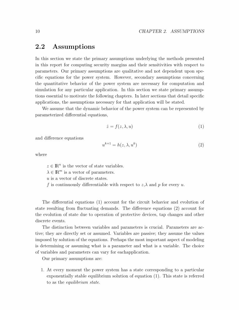
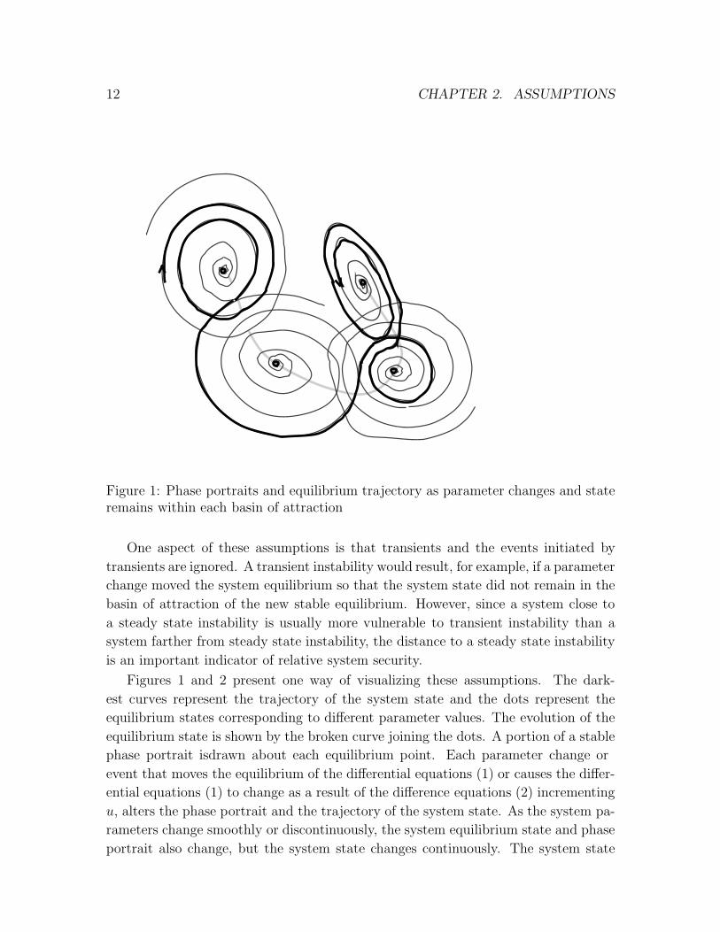
Figure 1: Phase portraits and equilibrium trajectory as parameter changes and stateremains within each basin of attraction
One aspect of these assumptions is that transients and the events initiated by
transients are ignored. A transient instability would result, for example, if a parameter
change moved the system equilibrium so that the system state did not remain in the
basin of attraction of the new stable equilibrium. However, since a system close to
a steady state instability is usually more vulnerable to transient instability than a
system farther from steady state instability, the distance to a steady state instability
is an important indicator of relative system security.
Figures 1 and 2 present one way of visualizing these assumptions. The dark-
est curves represent the trajectory of the system state and the dots represent the
equilibrium states corresponding to different parameter values. The evolution of the
equilibrium state is shown by the broken curve joining the dots. A portion of a stable
phase portrait is drawn about each equilibrium point. Each parameter change or
event that moves the equilibrium of the differential equations (1) or causes the differ-
ential equations (1) to change as a result of the difference equations (2) incrementing
u, alters the phase portrait and the trajectory of the system state. As the system pa-
rameters change smoothly or discontinuously, the system equilibrium state and phase
portrait also change, but the system state changes continuously. The system state
2.2. ASSUMPTIONS 13
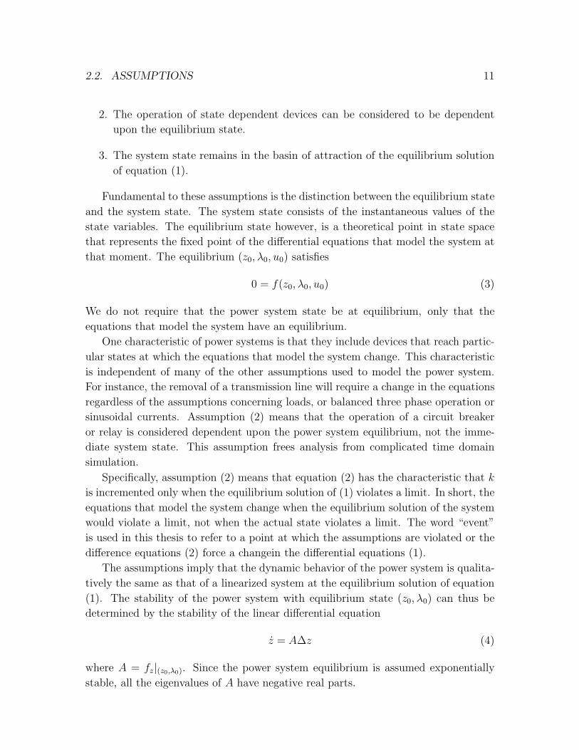
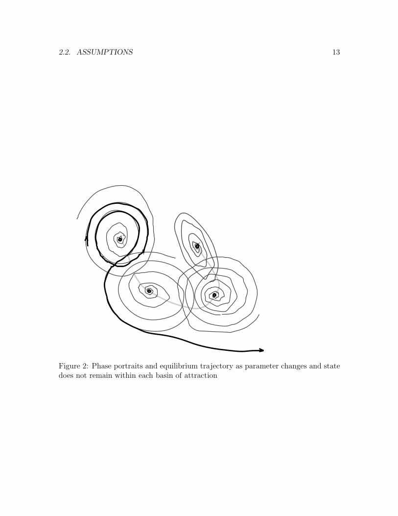
Figure 2: Phase portraits and equilibrium trajectory as parameter changes and statedoes not remain within each basin of attraction

14 CHAPTER 2. ASSUMPTIONS
in both figures initially spirals inward towards the top left equilibrium state. As the
parameters of the system change the equilibrium state of the power system moves
and the trajectory of the system state is altered. The trajectory of the system state
is the transient response of the system to the parameter disturbances. In Figure 1,
the system state remains in the basin of attraction of each equilibrium and traces a
portion of the phase portrait corresponding to each equilibrium. The behavior illus-
trated in Figure 2 does not satisfy the assumptions since the system state does not
remain in the basin of attraction of each equilibrium.
The main assumption required by the methods of this thesis is that the qualitative
behavior of the system state can be determined by analysis of the equilibrium state.2 The complicated trajectory of the system state is not modeled. The analysis of
stability based on the equilibrium state is classified as static stability or steady-state
stability analysis to distinguish it from transient or dynamic stability analysis. This
classification has sometimes led to confusion since some researchers assume that if
a dynamic phenomena is observed, a transient model must be required for analysis.
However, the consequence of a static instability is dynamic. The distinction between
static and dynamic analysis does not concern the consequences of the instability or
phenomena observed but rather the nature of the assumptions employed for analysis.
By locating the parameters λ at which the assumptions break down, we identify
not only the limits of the model but also a boundary at which reliable operation of
the actual power system is unlikely. The model breaks down by only four generic
mechanisms:
1. The stable equilibrium solution disappears as parameters change.
2. The stable equilibrium solution disappears as the difference equations change
the differential equations.
3. The stable equilibrium solution becomes unstable as parameters change.
4. The stable equilibrium solution becomes unstable as the difference equations
change the differential equations.
2These assumptions differ slightly from the often cited quasi-static steady state assumption[VC94, LofPhD, DC89]. One common description of the quasi-static steady state assumption isthat the parameter vector changes slowly compared to the dynamics of the system, so that thesystem state approximately traces a locus of stable equilibria. The quasi-static steady state assump-tions satisfy our assumptions but are stronger. We also allow parameters to occupy discrete statesand hence they change discretely, not necessarily slowly. However, we assume that the state remainsin the basin of attraction of the new stable equilibrium. The term “quasi-static steady state” is alsosometimes cited as justification for the standard load flow equations which assume that the powersystem voltages and currents are sinusoidal of constant frequency.
2.2. ASSUMPTIONS 15
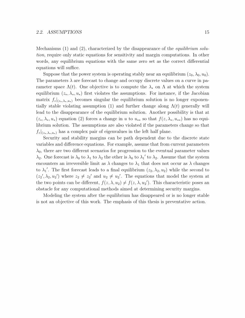
Mechanisms (1) and (2), characterized by the disappearance of the equilibrium solu-
tion, require only static equations for sensitivity and margin computations. In other
words, any equilibrium equations with the same zero set as the correct differential
equations will suffice.
Suppose that the power system is operating stably near an equilibrium (z0, λ0, u0).
The parameters λ are forecast to change and occupy discrete values on a curve in pa-
rameter space Λ(t). One objective is to compute the λ∗ on Λ at which the system
equilibrium (z∗, λ∗, u∗) first violates the assumptions. For instance, if the Jacobian
matrix fz|(z∗,λ∗,u∗) becomes singular the equilibrium solution is no longer exponen-
tially stable violating assumption (1) and further change along Λ(t) generally will
lead to the disappearance of the equilibrium solution. Another possibility is that at
(z∗, λ∗, u∗) equation (2) forces a change in u to u∗∗ so that f(z, λ∗, u∗∗) has no equi-
librium solution. The assumptions are also violated if the parameters change so that
fz|(z∗,λ∗,u∗) has a complex pair of eigenvalues in the left half plane.
Security and stability margins can be path dependent due to the discrete state
variables and difference equations. For example, assume that from current parameters
λ0, there are two different scenarios for progression to the eventual parameter values
λ2. One forecast is λ0 to λ1 to λ2 the other is λ0 to λ1′ to λ2. Assume that the system
encounters an irreversible limit as λ changes to λ1 that does not occur as λ changes
to λ1′. The first forecast leads to a final equilibrium (z2, λ2, u2) while the second to
(z2′, λ2, u2
′) where z2 6= z2′ and u2 6= u2
′. The equations that model the system at
the two points can be different, f(z, λ, u2) 6= f(z, λ, u2′). This characteristic poses an
obstacle for any computational methods aimed at determining security margins.
Modeling the system after the equilibrium has disappeared or is no longer stable
is not an objective of this work. The emphasis of this thesis is preventative action.

16

17
Chapter 3
Margin Computations
This chapter contains a comprehensive explanation of methods to compute margins in
electric power systems. Path following methods have found widespread use in power
systems analysis; this chapter represents a synthesis of several different perspectives
and suggests improvements and extensions to previous implementations. The presen-
tation of the material in this chapter is original and is intended to give insight into
the relation between the computational methods and the power system model.
3.1 Previous work
The practical use of path-following or continuation methods for tracing equilibrium
solutions for power systems analysis most likely predates the first publication of such a
method in the power systems literature. Continuation methods for locating the point
of voltage collapse of power systems have been presented in [Iba, AC92, CA93, CFSB]
and utilized in [GDA97, GDA98, RHSC, VC91]. [Seydel] includes a direct method
for locating a saddle node bifurcation. Similar methods for computing the margin to
voltage collapse are demonstrated in [AJ89, DL192].
The use of steady state continuation programs is now well established and expla-
nation of the “continuation power flow” method appears in the recent power systems
text [Kundur]. Continuation methods can be implemented with any set of power
system equilibrium equations although common descriptions of the programs often
assume the standard power flow equations. [VC94, VC96] use a continuation program
with elaborate equilibrium equations. [DV93] and [LAH95] present other examples of
more detailed equilibrium equations that could also be used in continuation methods.
(See the discussion by Canizares in [LAH95].)
The main ingredients of the material in this chapter are fundamental and well
explained in the texts [Seydel] and [GZ].

18 CHAPTER 3. MARGIN COMPUTATIONS
3.2 Anatomy of margin computations
This section describes methods for computing security margins given a model that
satisfies the assumptions stated in Chapter 2. The problem of computing a security
margin to an event involves finding an equilibrium that satisfies a specific condition.
For example, the condition can be that the equilibrium have a particular variable at a
threshold value, or that the system Jacobian matrix be singular at that equilibrium.
The fundamental problem en route to establishing a security margin is the solution
for a new equilibrium resulting from a specific change in the parameters. Typically,
a forecast of the parameter values at a future time is available without an exact
description of how the parameters progressed to those values. Ideally, the solution
obtained is an equilibrium corresponding to the forecast parameter values that is
connected by a curve of equilibria to the known solution for some reasonable pattern
of parameter variation connecting the current and forecast parameter values. The
solution must satisfy the equilibrium equations, not violate any limits, and lie on a
curve that satisfies the equilibrium and limit conditions for some curve connecting
the current and future parameter values. Unfortunately, even given two equilibrium
points that satisfy the same limit constraints, it is not possible to verify that they are
indeed solutions that satisfy these conditions without very specific restrictions on the
equilibrium equations. See [GZ] for illustrations of what can go wrong. The situation
is complicated even more by the inclusion of limits that can change the form of the
equilibrium equations. We instead first address the solution to a simpler problem
that ignores any limits.
Problem 1 (Simple)
Given : Find : z1 such that
(z0, λ0)
F (z0, λ0) = 0
λ1
(F (z1, λ1) = 0
)
An effective and time-tested method for solving Problem (1) is Newton’s method.
Method 1 (Newton) 1
Begin: z1 → z0
1Notation: Several concepts in this chapter are illustrated with pseudo-code. Superscripts referto iterations, so that zk is the value stored for z after k iterations. Subscripts refer to either initialor final values corresponding to the problem statements. The → should be read as “gets the value”so that a → b means a gets the value b. The expression x → Ax = b means that x gets the valuethat solves Ax = b.

3.2. ANATOMY OF MARGIN COMPUTATIONS 19
While: (|F (zk, λ1)| > tolerance) and (iterations < max)
Do:∆z → Fz|(zk,λ1)∆z = −F (zk, λ1)
zk+1 → zk + ∆z
If ( |F (zk, λ1)| < tolerance ) then z1 → zk, else warning
Many variants exist. For example, the elements of Fz can be updated only every
few iterations (Very Dishonest Newton). In some cases Fz is approximated. There
are many ways to solve the linear system in the iterative step [GV], some invented
specifically for power systems applications [Sto74], like the popular fast decoupled load
flow.
In general there is no guarantee that a solution exists or that the initial guess will be
sufficiently close to it to get convergence within a reasonable number of iterations.
The method may fail for several possible reasons:
1. A solution exists but the initial guess z0 was not close enough to the solution
for the method to converge, or converge fast enough.
2. There is no solution of F (z, λ1) = 0 (previous fold bifurcation for λ < λ1).
3. A solution exists but the method converged to the wrong solution, a solution
on another branch of equilibria.
However, if a solution exists and F is continuously differentiable and regular in a
neighborhood about the solution, the algorithm is guaranteed to converge to the
solution for an initial guess in some neighborhood of that solution(see [GZ] for proof).
Thus, it is prudent to modify Method (1) to improve the initial guess.
Method 2 (Newton with predictor) This method uses a tangent linear approx-
imation to start the Newton iteration. The initial step is often referred to as the
predictor step. Variants exist that use quadratic predictors and predictors that require
more than one previous solution [GZ].
Begin:Zλ → Fz|(z0,λ0)Zλ = −Fλ|(z0,λ0)
z1 → z0 + Zλ(λ1 − λ0)
While: (|F (zk, λ1)| > tolerance) and (iterations < max)
Do:∆z → Fz|(zk,λ1)∆z = −F (zk, λ1)
zk+1 → zk + ∆z
If ( |F (zk, λ1)| < tolerance ) then z1 → zk, else warning

20 CHAPTER 3. MARGIN COMPUTATIONS
Note that for the case when λ appears linearly in F , this method is exactly equivalent
to Method (1) except that the first iteration is performed outside of the loop.
As before, convergence is still not guaranteed and Method (2) can fail for all the
same reasons as Method (1). If the method fails to converge we may restart it for
a different choice of λ1 closer to λ0. However, what if the method converged to the
wrong solution? Can a wrong solution be detected?
In practice, power systems engineers believe that by inspecting the voltage magni-
tudes they can tell if a solution is reasonable2. This suggests a simple way to improve
the method so that convergence to a reasonable solution is more likely. Instead of
solving F (z, λ1) = 0, we solve an augmented set of equations
(F (z, λ)
C(z, λ)
)= 0. The
zero set of the map C specifies a desired characteristic of the solution. For example,
if it was expected that the voltage at a particular bus would drop due to increases in
loading, C can specify a voltage at that bus lower than its present voltage. Rather
than solve for the state corresponding to a specified loading, the loading that corre-
sponds to the specified characteristic of the state is found. Instead of being a fixed
parameter of the solution method, λ is an unknown and λ1 is an initial guess for λ.
Hence, C(z, λ) must include enough equations to allow for the solution of λ. When
λ is multidimensional, λ1 can define a direction from λ0 and the step size in that
direction then is an unknown.
Method 3 (Newton with predictor and corrector) This example uses a par-
ticular corrector so that the state variable with the largest predicted change is fixed at
its linearly predicted value. This method is the basic step employed by [AC92].
Begin:∆λ→ (λ1 − λ0)
k → ∆λ/|λ|Zλ → Fz|(z0,λ0)Zλ = −Fλ|(z0,λ0)
z1 → z0 + Zλ∆λ
i→ Zλ∆λ(i) = Maxi (Zλ∆λ)
2The following discussion is from “Sparseness in Power Systems Equations” in [Reid]:
Larcombe: Power flow equations are nonlinear and so will in general have severalsolutions. How do you ensure that you have the correct solution?
Baumann: This is a difficulty and the analysis that is available is rarely helpful.We usually start with a solution having the same voltage value at each node in thehope of finding a solution with small voltage differences, a feature that the engineersregard as desirable.

3.2. ANATOMY OF MARGIN COMPUTATIONS 21
While: ( |F (zk, λk)| > tolerance ) and (iterations < max)
Do:(
∆z
∆s
)→
(Fz|(zk,λk) Fλ|(zk,λk)ke(i) 0
) (∆z
∆s
)=
(−F (zk, λk)
zk(i)− z1(i)
)
sk+1 → sk + ∆s
λk+1 → λk + ∆sk
If( |F (zk, λk)| < tolerance ) then (z∗, λ∗) → (zk, λk) else warning
Note that since zk(i) − z1(i) = 0 ∀ k ≥ 1, the corrector fixes the i − th variable for
all iterations. Essentially, the selected variable is treated as a parameter, and the
original parameter is treated as a variable. This process of selecting a variable to fix
is sometimes referred to as the parameterization step.
Since the predictor-corrector will converge to a solution for a λ∗ different than the
desired λ1, to solve problem (1) the method needs to be repeatedly run until λ∗ is
within tolerance of the desired λ1. However, most often the goal is to find the λ that
corresponds to some particular event anyway, and λ1 represents the first estimate of
the parameters at that event.
When Fz is nearly singular evaluated at any point during the iteration, Methods
(1) and (2) require solution of an ill conditioned linear system and are thus unstable
and prone to generate numerical errors. However, the Jacobian matrix
(Fz FλCz Cλ
),
not Fz, determines the condition of the predictor-corrector method. For a properly
chosen (Cz, Cλ) numerical instabilities caused by a singular Fz are avoided.
Thus, the appended corrector equation has two beneficial effects. Not only does
it decrease the chances of convergence to an unacceptable solution, but the appended
row improves the conditioning of the Jacobian matrix used in the iterative step.
To find equilibrium solutions very close to or at fold bifurcations of F (z, λ) = 0, a
corrector should be used so that the linear system remains well conditioned even for
Fz singular. It is possible then to avoid numerical instability associated with the
singularity of Fz, and the trajectory of the equilibrium as a parameter is varied can
be traced right around a fold bifurcation.
The process of selecting a corrector equation can be thought of as appending rows
to the Jacobian matrix, not necessarily appending equations to be solved. For exam-
ple, one popular option [CA93, DeM96] is to choose (Cz, Cλ) as the vector orthogonal
to the initial tangent prediction, which is equivalent to selecting C so that (Cz , Cλ)
is a vector in the null space of (Fz, Fλ)T . Note that frequently it is advantageous
to expand the number of state variables to improve sparsity [Alv97] or to locate a
solution with a particular condition such as a bifurcation.
22 CHAPTER 3. MARGIN COMPUTATIONS
Sometimes the process of selecting the corrector equations is referred to as the pa-
rameterization step [CA93], and it can be performed after the predictor step [AC92]
or after the corrector if another equilibrium is to be found [CA93]. The entire method
is then the “predictor-corrector-parameterization” method. 3 The predictor-corrector
or predictor-corrector-parameterization method is the building block of path follow-
ing methods for power systems. If the continuation parameter reflects the actual
time evolving system parameters, the continuation method can be used as a “static
simulator” of the power system, tracing the progression of the system equilibrium.
Alternatively, continuation methods may also be used to trace a set of equilibria that
satisfy some other characteristics such as an operational boundary. In either case,
discrete device operation and limits, realistic parameter forecasts, and interarea and
generator dispatch policy must be accounted for.
It is frequently the case that solution for an equilibrium after a discrete parameter
change will force several limits to be violated. The most common solution then is
to fix one limit at a time and resolve, starting with the most severely violated limit.
Although this method is simple and well accepted, there is no guarantee that the solu-
tion obtained represents a realistic power system equilibrium. For some applications
it is important to identify the order in which the limits are encountered.
The process of applying limits as the system equilibrium evolves needs careful
attention. The operation of the power system changes in response to approaching
and encountering limits. The response to one limit may affect which limits will occur
next. The limits encountered and thus the equations that model the system at any
point are dependent upon the path the system followed to reach that point. Thus,
security margins are path dependent.
For some parameters and applications, it is reasonable to assume that λ evolves in
a piecewise linear manner. For example, from λ0 the parameters are forecast to change
to λ1, and λ may successively occupy discrete values that lie on a ray connecting λ0
to λ1. If the discrete values are close enough together, or if λ changes continuously,
the order that limits are encountered under the assumptions is well defined4.
The repeated objective of a program to trace the equilibrium state of the system as
parameters change in a quasi-continuous piecewise linear pattern is to find the relevant
equilibrium corresponding to the next limit event. Method (3) requires adjustment
for use in a continuation method that accounts for limit events. Essentially, the core
problem to be solved is to find each λ that forces the equilibrium equations to change
3The term “corrector” is usually used to refer to the iterative loop itself, so that methods (1)and (2) are technically predictor-corrector methods as well.
4Of course, the assumptions may not reflect reality. Although we can compute a precise order ofevents under our assumptions, the actual timing may depend on transient effects.

3.2. ANATOMY OF MARGIN COMPUTATIONS 23
due to a limit en route to finding a solution at some maximum forecast parameters.
Problem 2 (Find the next event) Zlim is a vector of limits.
Given : Find : (z∗, λ∗) such that
(z0, λ0, u0)
f(z0, λ0, u0) = 0
F (z, λ) = f(z, λ, u0)
z0 < Zlim
λ1
z∗<= Zlim
z∗[i] = Zlim[i]
F (z∗, λ∗) = 0
OR(z∗ < Zlim
F (z∗, λ1) = 0
)
One possible solution to problem (2) is to use method (3) with the orthogonal
corrector or parameterization step in an interval halving approach. For an initial
guess of λ1, method (3) is used to find another equilibrium. If a limit is not violated
λ is increased and the process repeated until a solution that violates a limit is found
or a solution at λ1 is obtained. If a limit is violated before that, we can then decrease
λ to the midpoint between the last no-limit solution and the first post-limit solution,
eventually finding a point within tolerance of the exact point where the first limit is
reached. The idea is that if you take small enough steps and find a pre-limit point
that is reasonably similar to an acceptable starting point, and then a point with only
one limit violated reasonably close to the pre-limit point, that one limit is likely to
be the next limit. However, the interval halving approach may require an excessive
number of solutions.
An improvement is made by modifying the predictor step of method (3) to predict
the next limit, and then select a corrector to solve directly for the point at which that
limit is reached. The resulting method will exactly locate the parameter and state
corresponding to the next predicted event such as a line flow or bus voltage reaching
an operational limit. For example, if I is the magnitude of a line current of interest
and Imax the limit, the corrector equation would be E(z, λ) = I − Imax.
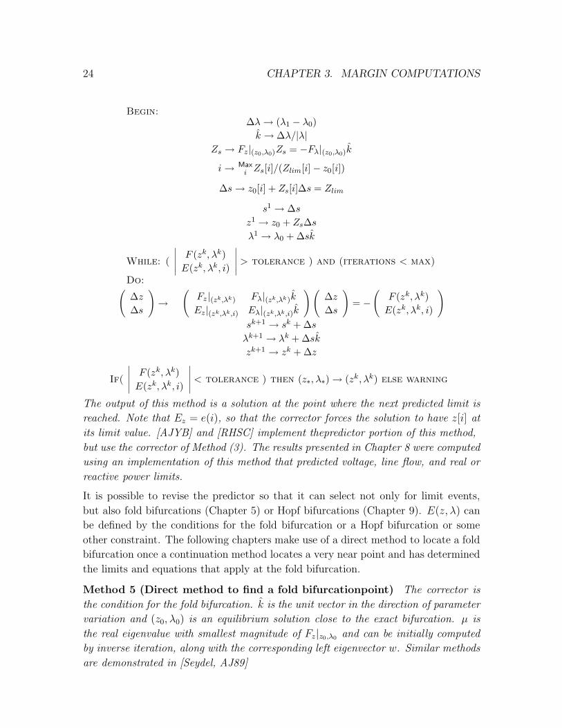
Method 4 (Direct method to locate the next event) Zlim is a vector of the
maximum limits of the z variables. The corrector is selected to be the linearly predicted
next limit event. E(z, λ, i) = z[i]− Zlim[i]
24 CHAPTER 3. MARGIN COMPUTATIONS
Begin:∆λ→ (λ1 − λ0)
k → ∆λ/|λ|Zs → Fz|(z0,λ0)Zs = −Fλ|(z0,λ0)k
i→ Maxi Zs[i]/(Zlim[i]− z0[i])
∆s→ z0[i] + Zs[i]∆s = Zlim
s1 → ∆s
z1 → z0 + Zs∆s
λ1 → λ0 + ∆sk
While: (
∣∣∣∣∣F (zk, λk)
E(zk, λk, i)
∣∣∣∣∣ > tolerance ) and (iterations < max)
Do:(
∆z
∆s
)→
(Fz |(zk,λk) Fλ|(zk,λk)k
Ez|(zk,λk,i) Eλ|(zk,λk,i)k
) (∆z
∆s
)= −
(F (zk, λk)
E(zk, λk, i)
)
sk+1 → sk + ∆s
λk+1 → λk + ∆sk
zk+1 → zk + ∆z
If(
∣∣∣∣∣F (zk, λk)
E(zk, λk, i)
∣∣∣∣∣ < tolerance ) then (z∗, λ∗) → (zk, λk) else warning
The output of this method is a solution at the point where the next predicted limit is
reached. Note that Ez = e(i), so that the corrector forces the solution to have z[i] at
its limit value. [AJYB] and [RHSC] implement the predictor portion of this method,
but use the corrector of Method (3). The results presented in Chapter 8 were computed
using an implementation of this method that predicted voltage, line flow, and real or
reactive power limits.
It is possible to revise the predictor so that it can select not only for limit events,
but also fold bifurcations (Chapter 5) or Hopf bifurcations (Chapter 9). E(z, λ) can
be defined by the conditions for the fold bifurcation or a Hopf bifurcation or some
other constraint. The following chapters make use of a direct method to locate a fold
bifurcation once a continuation method locates a very near point and has determined
the limits and equations that apply at the fold bifurcation.
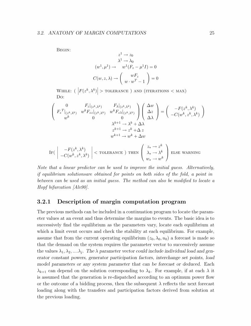
Method 5 (Direct method to find a fold bifurcation point) The corrector is
the condition for the fold bifurcation. k is the unit vector in the direction of parameter
variation and (z0, λ0) is an equilibrium solution close to the exact bifurcation. µ is
the real eigenvalue with smallest magnitude of Fz|z0,λ0 and can be initially computed
by inverse iteration, along with the corresponding left eigenvector w. Similar methods
are demonstrated in [Seydel, AJ89]
3.2. ANATOMY OF MARGIN COMPUTATIONS 25
Begin:z1 → z0λ1 → λ0
(w1, µ1) → w1(Fz − µ1I) = 0
C(w, z, λ) →(
wFzw ·wT − 1
)= 0
While: (∣∣∣F (zk, λk)
∣∣∣ > tolerance ) and (iterations < max)
Do:
0 Fz|(zk,λk) Fλ|(zk,λk)Fz
T |(zk,λk) wkFzz|(zk,λk) wkFzλ|(zk,λk)wk 0 0
∆w
∆z
∆λ
=
(−F (zk, λk)
−C(wk, zk, λk)
)
λk+1 → λk + ∆λ
zk+1 → zk + ∆z
wk+1 → wk + ∆w
If(
∣∣∣∣∣−F (zk, λk)
−C(wk, zk, λk)
∣∣∣∣∣ < tolerance ) then
z∗ → zk
λ∗ → λk
w∗ → wk
else warning
Note that a linear predictor can be used to improve the initial guess. Alternatively,
if equilibrium solutions are obtained for points on both sides of the fold, a point in
between can be used as an initial guess. The method can also be modified to locate a
Hopf bifurcation [Alv90].
3.2.1 Description of margin computation program
The previous methods can be included in a continuation program to locate the param-
eter values at an event and thus determine the margins to events. The basic idea is to
successively find the equilibrium as the parameters vary, locate each equilibrium at
which a limit event occurs and check the stability at each equilibrium. For example,
assume that from the current operating equilibrium (z0, λ0, u0) a forecast is made so
that the demand on the system requires the parameter vector to successively assume
the values λ1, λ2, ....λj. The λ parameter vector could include individual load and gen-
erator constant powers, generator participation factors, interchange set points, load
model parameters or any system parameter that can be forecast or deduced. Each
λk+1 can depend on the solution corresponding to λk. For example, if at each λ it
is assumed that the generation is re-dispatched according to an optimum power flow
or the outcome of a bidding process, then the subsequent λ reflects the next forecast
loading along with the transfers and participation factors derived from solution at
the previous loading.
26 CHAPTER 3. MARGIN COMPUTATIONS
Assume that the forecast provides a piecewise linear estimate of the projected
actual parameter change. In other words, the actual parameter change is forecast to
successively occupy the discrete values λi as well as intermediate values that lie on
lines connecting the λi. Each increment defines a direction of parameter change. The
first direction is k1 = (λ1 − λ0)/|(λ1 − λ0|. The first objective of the program is to
find the equilibrium corresponding to λ1 – the problem we have already addressed.
Several intermediate equilibria corresponding to λ = λ0 + sk1 for s < 1 may be
found as well, especially when those parameter values correspond to limit events.
The process is repeated to find the equilibrium corresponding to λ2 and so on, until
equilibria corresponding to each forecast λ are found, or until an equilibrium at which
the system loses stability is found.
Method 6 (Generic power systems continuation method) Continuation method
to find steady state instability or security limits.
Begin: Obtain state including limits, and forecast parameter changes,
(λ1, λ2, ..., λn).
While (stable and secure) and (λ 6= λn)
Do:
While (stable and secure) and (λ 6= λj)
Do:
1. Call predictor-corrector (corrector determined by
the linear estimate of the next event), return new
equilibrium and at most one limit.
2. Check stability.
3. If stable, apply limit, check stability.
increment j
The output of the program is either the final state at the last forecast parameter values,
or the state and parameters at which the system loses stability or violates a security
constraint.
When the parameter forecast is based on a realistic time evolution of the actual
parameters, the program can be viewed as a static simulator of the power system.
However, there are good uses for parameter forecasts that do not reflect the time
evolution of parameters. Chapter 6 uses this method to determine a theoretical post-
contingency steady state, where λ represents line admittance. Similarly, λ may rep-
resent interchange set points and Method (6) can be used to determine the interarea
transfer boundary at a specific loading level. Thus Method (6) is both a simulation
tool and a computational tool.

3.3. SUMMARY 27
This method has now been successfully implemented with a 1500 bus model for a
major US utility, and used to determine the loading and transfer margins to events at
which system costs increase discretely. The model predicts and finds real and reactive
power output limits, line flow limits, and voltage limits initiating switching operation
or violating security constraints. At each limit event, generation is redispatched
according to a Constrained Economic Dispatch (CED) to determine the next direction
of parameter variation.
Once method (6) has determined the point of instability or security limit violation,
a nominal margin to that event can be defined by the norm of the difference in
the parameter values at the current operating point and those at the event point.
The choice of norm is arbitrary and should be based on convenience and ease of
interpretation. If the current operating point is (z0, λ0, u0) and the point of instability
is (z∗, λ∗, u∗), λ∗−λ0 is a vector in parameter space. The length of the vector can be
measured in any norm.
In some instances, the margin is best measured in state space, not parameter space.
For example, assume that the instability is a Hopf bifurcation and that a detailed load
model was employed so that expressions for the real and reactive power at a bus were
dependent upon state variables (such as voltages and/or time derivatives of voltages).
In this case, the real and reactive powers are state variables, not parameters, but
operators may still wish to measure a margin to instability in real power since it is
easily monitored. In this case the margin can be defined by a norm of z∗ − z0. Note
that it may even be advantageous to measure norms in state and parameter space -
the norm of (z∗, λ∗)−(z0, λ0). One may even choose a measure in a discrete parameter
space; for example, the number of discrete events encountered between the current
operating point and loss of stability.
3.3 Summary
A conceptual continuation program for computing margins to events has been ex-
plained. The continuation program serves two purposes. On one hand, it is a com-
putational tool for locating specific equilibrium solutions, such as fold bifurcations or
limit violations. On the other hand, it is a system simulator, showing the evolution
of the system equilibrium as conditions are altered. The program uses a predictor-
corrector method to trace a curve of equilibria. The corrector serves two roles. First,
it improves the likelihood of convergence to an acceptable solution or a specific type
of solution. Second, it avoids problems due to a poorly conditioned or singular system
Jacobian matrix. The predictor also has two roles. First, it improves the initial guess
of the Newton step so that convergence to a correct solution is more likely. Second,

28 CHAPTER 3. MARGIN COMPUTATIONS
it determines which corrector to use by indicating what the likely next event is.
Suppose that the margin to some event has been computed. How would the
margin change if some parameter was different than forecast? Will it be necessary to
recompute another continuation to find the new margin? This question is answered
in Chapter 4.
Chapter 4
Sensitivity Computations
Chapter 3 described how the security margin to an event boundary could be efficiently
computed by using a corrector that specified the event condition. Once the solution
at an event is obtained in this manner the sensitivity of the margin to that boundary
with respect to almost every power system parameter can be obtained for very little
additional computational cost. This chapter explains and derives the formula for the
sensitivity of a margin with respect to an arbitrary parameter vector.
Suppose that we are interested in locating the point where the power system volt-
ages become unacceptably low due to the gradual increase in demand along some
forecast pattern. The continuation program can trace a curve of equilibria as de-
mand increases, locating intermediate limits that initiate tap changing or generator
protection, until the point where the first low voltage limit occurs is found. The
continuation program may have assumed a particular interarea transfer or pattern
of transfers. How much can the transfer be adjusted without significantly impacting
the margin to a low voltage event? By how much will the load at which that limit is
encountered change for a different transfer?
4.1 Methods of sensitivity analysis
The brute force way to answer the previous questions is as follows. At the initial
operating point, we alter the interarea transfers as proposed and find the correspond-
ing equilibrium. Next, the continuation method is used as before to locate the new
first voltage limit. If several possible changes to the interarea transfer are under
consideration, several continuations are run. This method is outlined below.
Method 7 (Multiple Continuations)
Brute force method to compute points on an event boundary.
Begin: Obtain initial state, parameters, forecast, and control
parameter values (p0, p1, ..., pn).
While (p 6= pn)
Do:
29
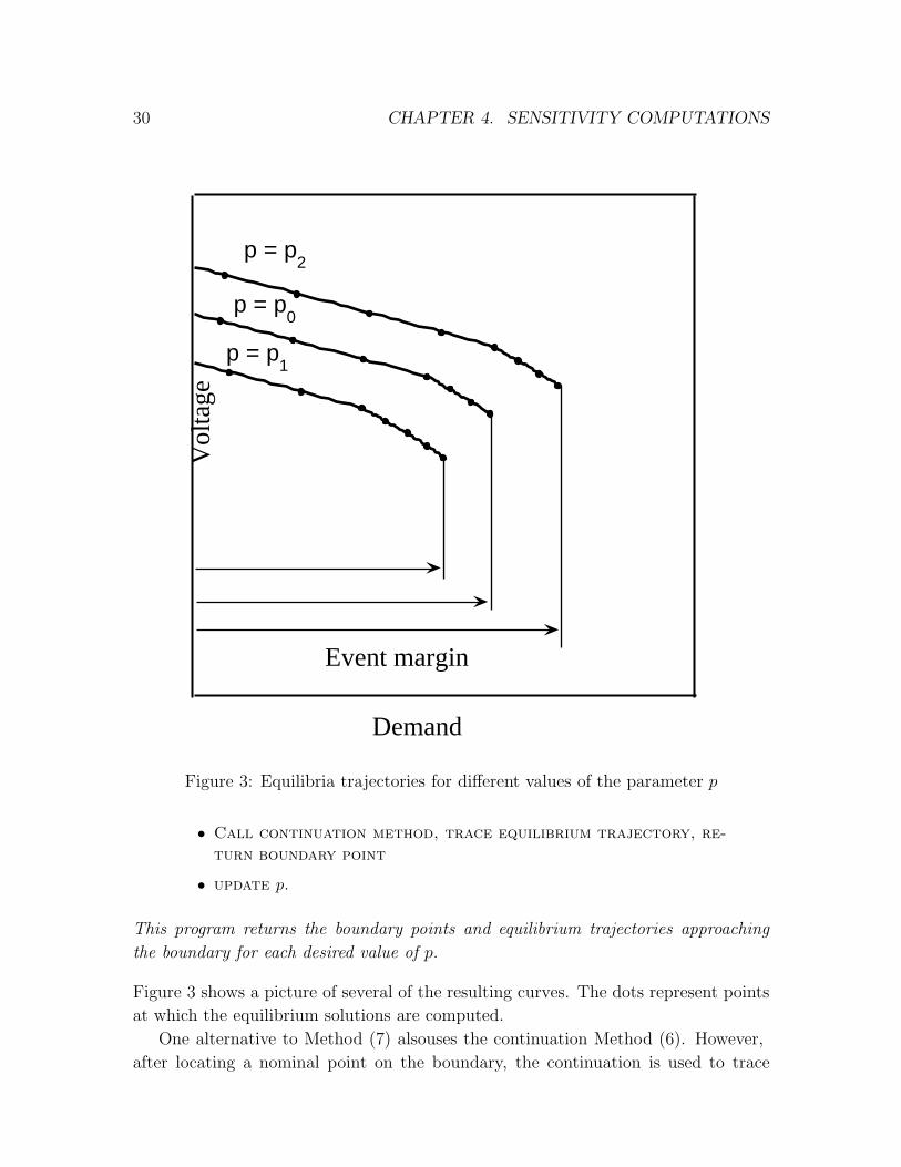
30 CHAPTER 4. SENSITIVITY COMPUTATIONS
Vol
tage
Demand
p = p1
Event margin
p = p0
p = p2
Figure 3: Equilibria trajectories for different values of the parameter p
• Call continuation method, trace equilibrium trajectory, re-
turn boundary point
• update p.
This program returns the boundary points and equilibrium trajectories approaching
the boundary for each desired value of p.
Figure 3 shows a picture of several of the resulting curves. The dots represent points
at which the equilibrium solutions are computed.
One alternative to Method (7) also uses the continuation Method (6). However,
after locating a nominal point on the boundary, the continuation is used to trace

4.1. METHODS OF SENSITIVITY ANALYSIS 31
a portion of the boundary starting from the nominal boundary point. The control
parameter becomes the continuation parameter and a locus of equilibria at which
the limit voltage is encountered is traced. The method is outlined below. [HD95]
implements this method for a small power system. (This method was also suggested
by Canizares in the discussion to [GDA97]).
Method 8 (Boundary Trace) Use the continuation method to find points on a
curve situated on the boundary around a nominal boundary point.
Begin: Obtain initial state, parameters, forecast, and control
parameter p.
Call continuation method to locate nominal boundary point and
condition.
While ( step change > min ) and (p 6= pmax)
Do:
1. Call predictor-corrector routine (corrector is the event
condition at the nominal point), return new equilibrium on
boundary.
2. Check limits.
3. If limits, reduce step change, else increase step
The program ends with either the control parameter at its maximum value and the
resulting change in the margin, or the maximum control parameter change and margin
corresponding to a point on the boundary where the limits in effect change.
Figure 4 shows the sequence of equilibria computed by Method (8) and the initial
continuation to find the nominal point on the boundary. This curve includes all the
boundary points computed by the previous method.
There is an alternative to either Method (7) or (8). Instead of computing addi-
tional points on the boundary, a Taylor series evaluated at the nominal boundary
point can be used to approximate the boundary. The first order Taylor series esti-
mate is equivalent to the initial predictor step that would be implemented by Method
(8). Second order and higher Taylor series approximations are possible, with the
higher order derivatives computed explicitly at the nominal point, or approximated
by computing one or more additional points on the curve. The Taylor series method
is outlined below.
Method 9 (Taylor series approximation) Compute one nominal boundary point,
estimate curve on the boundary.
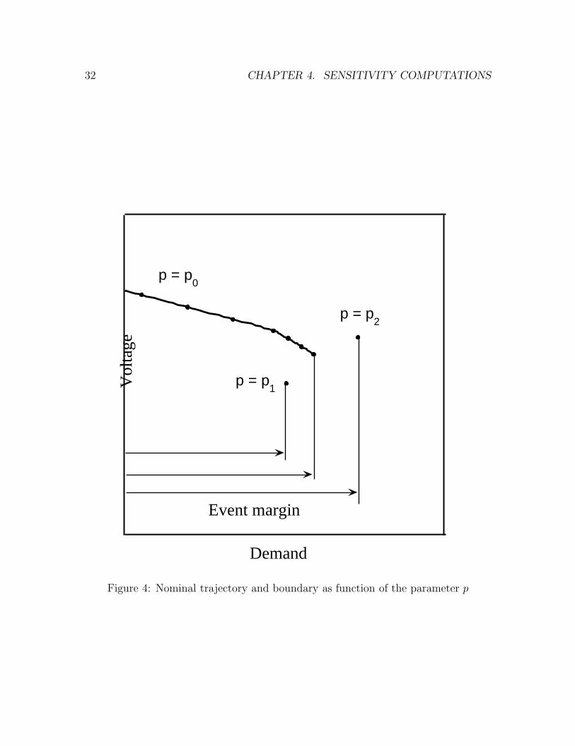
32 CHAPTER 4. SENSITIVITY COMPUTATIONS
Vol
tage
Demand
p = p1
Event margin
p = p0
p = p2
Figure 4: Nominal trajectory and boundary as function of the parameter p

4.1. METHODS OF SENSITIVITY ANALYSIS 33
Begin: Obtain initial state, parameters, forecast, and control
parameter p.
1. call continuation method to locate nominal boundary point.
2. compute derivatives of equilibrium and condition equations
with respect to p at boundary point.
3. Evaluate Taylor series estimates.
The output of this program is a Taylor series approximation of a curve on the boundary
evaluated for any value of p.
Figure 5 shows the Taylor series approximations to the boundary obtained from com-
putation of the nominal boundary point.
The advantage of Method (7) is that events that occur that differ from those of
the nominal continuation can be found en route to establishing the new margins. For
example, if for a given change to the control parameter, a different limit is reached
than for the nominal case, this will be detected. The disadvantage is that each
continuation is time consuming. The advantage of the Method (8) is time savings;
one computes exactly the equilibria of interest. The drawback is that if the change in
parameters changes the events encountered en route to the boundary, the results will
be incorrect and the computation a waste of time. Method (8) partially screens for
this by examining the solutions for limit violations on the boundary1. Method (9) is
less accurate than either continuation approach, but offers the greatest time savings
by many orders of magnitude. Approximate curves for many different parameters can
be computed faster than the exact computation of one curve for one parameter. The
first order Taylor series estimate is always much faster than the other methods since
the first order term is essentially the same as one predictor step. The second order
Taylor series is only worth computing if it is faster than computing a second point
on the boundary (since it is simple to fit a quadratic with two points and a tangent
vector).
Another advantage of Method (9) is that the sensitivity formulas are similar for
any parameter. Thus, if the formulas are evaluated for one parameter they can be
reevaluated for a different parameter at only a fraction of the cost to compute the
first sensitivity. The greater the number of parameters of interest, the greater the
computational savings of Method (9) over Method (8). In addition, the sensitivity
formulas are also useful for determining immediate control action.
1Note that this screening could only detect new limits violated on the boundary, not changesin the order of the limits encountered or limits that should no longer be enforced. For example, achange in the parameter p may cause a previous limit to not be encountered, and thus the equationsused to trace the boundary may not be valid yet the solutions would appear to satisfy the limitconditions.

34 CHAPTER 4. SENSITIVITY COMPUTATIONS
Vol
tage
Demand
∆ p = p1 - p
0
Estimated event margin
p = p0
∆ p = p2 - p
0
Figure 5: Nominal trajectory and estimated boundary
4.2. SENSITIVITY FORMULAS 35
4.2 Sensitivity formulas
This section presents derivations of the formulas for the sensitivity of margins to
events with respect to arbitrary parameters.
4.2.1 Derivation
Assume that (z0, λ0, u0) is a stable operating point where z ∈ IRn and λ ∈ IRm. The
continuation program determines that the point (z∗, λ∗, u∗) corresponds to an event
for variation of the λ parameters in the direction k. Let k be a unit vector in the
norm used to measure the margin.
k = (λ∗ − λ0)/|λ∗ − λ0| (5)
The security margin M to the event is M = |λ∗ − λ0|.The equilibrium equations valid at (z0, λ0, u0) are F (z, λ) = f(z, λ, u0). The
equilibrium equations valid at (z∗, λ∗, u∗) are F (z, λ) = f(z, λ, u∗). E(z, λ) defines
the event equation at (z∗, λ∗, u∗). For many limits, including voltage, flow, and power
limitations, defining the event equation E is simple. However, two events, the fold
and Hopf bifurcations, require special consideration and are discussed in sections 4.2.4
and 4.2.5 and detailed in Chapters 5 and 9 respectively. In general the selection of
the event equations E is analogous to selecting corrector equations C that allow for
direct solution of a boundary point.
Suppose that it is of interest how changing a selected parameter p changes the
state and remaining parameters at which the event described by E occurs. At the
nominal event point
(F (z∗, λ∗, p)
E(z∗, λ∗, p)
)= 0. Define the map H as
H(z, λ, p) =
(F (z, λ, p)
E(z, λ, p)
)(6)
The curve (if it exists) that Method (9) estimates is a subset of the set of equilibria
that satisfy the event conditions in state and parameter space around the nominal
boundary point. This set of equilibria, the preimage of the zero set of H, is denoted
H−1(0). Using calculus on H−1(0) is defensible only when H−1(0) is a differentiable
manifold. It turns out that for very general conditions this will indeed be true and
we are justified in the assumption that there are curves on H−1(0) that describe the
sets of interest to us. The conditions are
1. Hz|(z∗,λ∗) has rank n.

36 CHAPTER 4. SENSITIVITY COMPUTATIONS
2.(Hz Hλk
)∣∣∣(z∗,λ∗)
has rank n+ 1.
Condition (2) is a transversality condition stating that a vector through (z∗, λ∗) in
the k direction intersects H−1(0) transversally. Condition (1) can be interpreted as
a condition of uniqueness. Simply stated, Condition (1) specifies that only one event
occurs at a time. (Note that Condition 2 implies Condition 1. The redundancy
here is intentional and serves to distinguish between the restrictions on E and the
restrictions on k.) The details and implications of these conditions are addressed in
section 4.2.3. For now, assume that H−1(0) is a smooth manifold and a smooth curve
on that manifold parameterized by p is (Z(p),Λ(p)) so that (Z(p0),Λ(p0)) = (z∗, λ∗)
and (F (Z(p),Λ(p), p)
E(Z(p),Λ(p), p)
)= 0 (7)
Assume that p is not a component of λ. The more general case in which p is a
component of λ or λ depends on p is addressed in sections (4.2.2) and (4.2.3).
Since the system is assumed stable at the nominal operating point, Fz is nonsin-
gular as p is varied in a neighborhood about p0. Then as p is adjusted each new
equilibrium (Z(p), λ0, p), satisfying F (Z(p), λ0, p) = 0, can be associated with one
corresponding point (Z(p),Λ(p), p) satisfying H((Z(p),Λ(p), p)) = 0 that is the clos-
est point on H−1(0) in the direction k. The difference in parameter space between the
operating point (Z(p), λ0, p) and the corresponding boundary point (Z(p),Λ(p), p) is
Λ(p)− λ0 = L(p)k (8)
where L(p) is a scalar step in the k direction as a function of p. The margin as a
function of p is
M(p) = |Λ(p)− λ0| = |L(p)k + λ0 − λ0| = |L(p)k| (9)
Since k is a unit vector in the norm used for the margin, the margin as a function of
p is M(p) = L(p). Write Λ(p) in terms of the margin L(p)
Λ(p) = L(p)k + λ0 (10)
Equation (7) can then be written(F (Z(p), L(p)k + λ0, p)
E(Z(p), L(p)k + λ0, p)
)= 0 (11)
Differentiating (11) at (z∗, λ∗) with respect to p and applying the chain rule for
derivatives yields a linear system(Fz Fλk
Ez Eλk
)∣∣∣∣∣∗
(Zp
Lp
)= −
(FpEp
)∣∣∣∣∣∗
(12)
4.2. SENSITIVITY FORMULAS 37
The matrix
(Fz Fλk
Ez Eλk
)∣∣∣∣∣∗
is nonsingular by Condition 2.
Solution of (12) then yields Lp, the sensitivity of the security margin with respect
to p. The first order estimate of the change in margin corresponding to the change
in p of ∆p is
∆L = Lp∆p (13)
Solution of (12) additionally yields Zp, the tangent vector at (z∗, λ∗, p0) to the curve
in state space that describes how the state variables change to satisfy the equilibrium
and event conditions as p varies2. Thus, Zp∆p is the first order Taylor series estimate
of how the state changes on H−1(0) for a parameter change of ∆p.
Since the matrix
(Fz Fλk
Ez Eλk
)∣∣∣∣∣∗
is the same for any3 parameter p, once the matrix
is factored and the sensitivities obtained for one parameter, computing the sensitiv-
ities for any additional parameters only requires obtaining the derivatives
(FpEp
)∣∣∣∣∣∗
and one forward and backward substitution.
If obtaining Lp for many parameters is of primary interest, and there is no desire
to obtain Zp, then full solution of the linear system (12) is not necessary. Since any
set of n + 1 vectors in IRn are linearly dependent there is a non-zero vector w such
that
w
(FzEz
)∣∣∣∣∣∗
= 0 (14)
w is a vector orthogonal to the range of
(FzEz
)∣∣∣∣∣∗
and w is unique up to a scalar
multiplication when
(FzEz
)∣∣∣∣∣∗
is full rank, which is guaranteed by condition (1).
Pre-multiplying (12) by w yields
w
(Fλk
Eλk
)∣∣∣∣∣∗
Lp = −w(FpEp
)∣∣∣∣∣∗
(15)
w
(Fλk
Eλk
)∣∣∣∣∣∗
is not zero since
(Fz Fλk
Ez Eλk
)∣∣∣∣∣∗
is nonsingular, so (15) can be solved
2Zp∆p can thus be used to screen for cases where new limits would be violated (Zp∆p[i] > Zlim[i])
3The presentation assumes that k does not explicitly depend on p and that p is not a componentof λ. The appropriate formulas for these special cases are simply obtained by applying the ChainRule for derivatives (see Appendix 5.7.C).

38 CHAPTER 4. SENSITIVITY COMPUTATIONS
to obtain the sensitivity with respect to p of the margin to the event.
Lp = −w
(FpEp
)∣∣∣∣∣∗
w
(Fλk
Eλk
)∣∣∣∣∣∗
(16)
Note that regardless of the number of parameters under consideration, w needs to be
computed only once.
Higher order sensitivities
Higher order sensitivities of the security margin with respect to p are computed by
repeatedly differentiating (11) at (z∗, λ∗) with respect to p and solving linear sys-
tems of equations. Chapters 5, 6, and 7 use the quadratic sensitivity of the loading
margin to voltage collapse with respect to transmission line parameters to estimate
the effects of line outages. Quadratic sensitivities have found use in optimization
routines. [OloPhD] uses quadratic sensitivities to improve the rate of convergence of
an optimization process. Quadratic sensitivities are also used by [GSHT] for sensitiv-
ity analysis of optimal power flow solutions, and in [NorPhD] for operation of series
compensators.
4.2.2 Normal vector to the event boundary in parameter
space
The sensitivity of the security margin to changes in many parameters is effectively just
an indexing operation once the scaled normal vector is obtained. The normal vector to
the event boundary in parameter space defines to first order the proportions by which
all the parameters must vary to keep the equilibrium at the security boundary. The
normal vector is useful in determining the relative effectiveness of different parameters
on the security margin. Note that if a point on the security boundary is obtained
using a direct method that uses the E equations as corrector equations, obtaining the
normal vector requires only one additional forward and backward substitution using
the previously factored Jacobian matrix.
The vector w used to obtain the margin sensitivity formulas is used to define the
normal vector to the hypersurface in parameter space that represents the surface on
which parameters must vary so that the resulting equilibrium satisfies the event and
equilibrium conditions.

4.2. SENSITIVITY FORMULAS 39
Let (Z(p),Λ(p)) represent arbitrary smooth curves in state space and parameter
space parameterized by p which satisfy
H(Z(p),Λ(p), p) =
(F (Z(p),Λ(p), p)
E(Z(p),Λ(p), p)
)= 0 (17)
and (Z(p0),Λ(p0)) = (z∗, λ∗). The tangent vector (Z, Λ, P ) to the curve (Z(p),Λ(p), p)
at (z∗, λ∗, p0) satisfies(Fz Fλ FpEz Eλ Ep
)∣∣∣∣∣∗
Z
Λ
P
= 0 (18)
Pre-multiplying (18) by w yields
w
(Fλ FpEλ Ep
)∣∣∣∣∣∗
(Λ
P
)= 0 (19)
where w is found from (14). Equation (19) shows that the vector N
N = w
(Fλ FpEλ Ep
)∣∣∣∣∣∗
(20)
is orthogonal to the tangent vector (Λ, P ) at (λ∗, p0) for an arbitrary curve (Z(p),Λ(p), p)
satisfying (17).
4.2.3 General derivation
Preliminary Assumptions
Assume that (z0, λ0, p0) is a stable operating point, and that ∗ = (z∗, λ∗, p0) is the
nominal event point where z ∈ IRn and λ ∈ IRm. Let p represent the parameters of
interest, with p ∈ IRρ.
The smooth map Q : IRρ → IRm describes the explicit dependence of λ on p by
λ = Q(p). Note that Q(p) can be a constant function. Assume that in a neighborhood
V of (z0, λ0, p0), the map F : V → IRn is smooth and
F (z0, λ0, p0) = 0 (21)
Since λ depends explicitly on p,
F (z,Q(p), p) = 0 (22)
As the p parameters change, the stable equilibrium moves to satisfy the F equilibrium
equations. Since (z0, λ0, p0) is asymptotically stable by the assumptions of Chapter
40 CHAPTER 4. SENSITIVITY COMPUTATIONS
2, Fz is nonsingular in an open neighborhood of (z0, λ0, p0) contained in V . By
the Implicit Function Theorem there is a unique smooth map Z(p) defined on a
neighborhood of p0 so that Z(p0) = z0 and
F (Z(p), Q(p), p) = 0 (23)
We are interested in the point on the event boundary that corresponds to each stable
operating point. The λ parameters at the stable operating point depend explicitly
on the p parameters while the parameters corresponding to boundary points depend
implicitly and explicitly on the parameters p. Defining a direction in which to measure
the margin distinguishes between the proportions of each of the parameters that vary
explicitly and those that vary implicitly.
The margin M to the event is the distance between the stable operating point
and the nominal event point along a direction k. It is practical then to represent
λ in coordinates so that the margin to the event is the scalar difference in only
one coordinate. This coordinate then varies implicitly with p while the remaining
coordinates vary explicitly with p.
Let T : IRm → IRm represent a linear isomorphism from λ to (`, s), ` ∈ IR1 and
s ∈ IRm−1 where the columns of T form an orthogonal basis for IRm and ` represents
the projection of λ in the k direction so that
λ = T
(`
s
)=
(k K
) (`
s
)(24)
and (`
s
)= T−1λ (25)
The nominal margin then is
M = |T−1(λ∗ − λ0)| = `∗ − `0 (26)
To emphasize the dependence on p we write
(L(p), S(p)) = T−1Q(p) (27)
In addition, assume F and E are smooth maps in a neighborhood U of (z∗, λ∗, p0)
and that at the nominal event point(F (z∗, λ∗, p0)
E(z∗, λ∗, p0)
)= 0 (28)
Define the smooth map H : U → IRn+1
H(z, λ, p) =
(F (z, λ, p)
E(z, λ, p)
)(29)
and H(z∗, λ∗, p0) = 0
4.2. SENSITIVITY FORMULAS 41
Assumptions
1. Hz|∗ has rank n.
2.(Hz Hλk
)∣∣∣∗
has rank n+ 1.
Properties
1. H−1(0) is locally an m + ρ − 1 manifold in a neighborhood of (z∗, λ∗, p0) and
there exists a neighborhood U of p0 and unique smooth maps (Z(p),Λ(p)) so
that (Z(p0),Λ(p0)) = (z∗, λ∗) and p ∈ U implies that H(Z(p),Λ(p), p) = 0.
2. The set Σ = {(Λ(p), p) | p ∈ U} is an m + ρ − 1 manifold in IRm+ρ that is
diffeomorphic to H−1(0). The vector N = (wHλ, wHp)|∗, where w is given by
wHz|∗ = 0, is in the direction normal to Σ at (λ∗, p0). N is unique up to scalar
multiple.
3. The sensitivity of the margin M with respect to p is
Mp = Lp − Lp = −(wHp + wHλQp
wHλk
)∣∣∣∣∣∗
(30)
Proof
Assumption (2) implies that H is surjective at (z∗, λ∗) and by the Preimage Theorem
(pages 20 -21 [GP] ) H−1(0) is locally an m+ρ−1 manifold. Assumption (1) implies
that there exists a nonzero row vector w such that wHz |(z∗,λ∗) = 0 and w is unique
up to scalar multiple.
Define the smooth map G : IRn × IR1 × IRρ → IRn+1
G(z, `, p) = H(z,T(`, S(p)), p) (31)
The derivative of G with respect to (z, `) is (Hz, Hλk) and is nonsingular at (z∗, λ∗, p0)
by Assumption 2. By the Implicit Function Theorem there exists a neighborhood U
of p0 and unique smooth maps (Z(p), L(p)) so that (Z(p0), L(p0)) = (z∗, `∗) and p ∈ U
implies
G(Z(p), L(p), p) = 0 (32)
By the Preimage Theorem G−1(0) is a manifold. Since T is a diffeomorphism from
λ to (l, s) coordinates, H−1(0) is diffeomorphic to G−1(0). Let Λ(p) = T(L(p), S(p)).
Then
G(Z(p), L(p), p) = H(Z(p),Λ(p), p) = 0 (33)
and Property 1 is proved.

42 CHAPTER 4. SENSITIVITY COMPUTATIONS
Differentiating Equation (33) with respect to p yields
HzZp +HλΛp +Hp = 0 (34)
Pre-multiplying by w and evaluation at (z∗, λ∗, p∗) yields
wHλ|∗Λp + wHp|∗ = 0 (35)
showing that N = (wHλ, wHp)|∗ is normal to the manifold {(Λ(p), p) | p ∈ U} at
(λ∗, p0). N is nonzero by Assumption 2, so we can consider N a map from IRm×IRρ to
IR1 with a kernel spanned by m+ρ−1 basis vectors. Define the map Γ : IRm×IRρ → IR
Γ(λ, p) = wH(Z(p), λ, p) (36)
Assumption 2 implies that (Γλ,Γp)|∗ = (wHλ, wHp)|∗ is surjective. By the Preimage
Theorem, Σ = Γ−1(0) is an m+ρ−1 manifold with codimension 1. In a neighborhood
of (z∗, λ∗, p∗) Σ is diffeomorphic to H−1(0) since the map Π : H−1(0) → Γ−1(0) defined
by
Π(z, λ, p) = (λ, p) (37)
is one to one and onto and the inverse map
Ψ(λ, p) = (Z(p), λ, p) (38)
is smooth. Since Γ is constant on Σ, differentiating (36) with respect to (λ, p), evalu-
ating at (λ∗, p∗), and using wHz|∗ = 0 shows that (wHλ, wHp)|∗ is the normal vector
to Σ at (λ∗, p∗) and Property 2 is proved.
Define the map G : IRn × IRρ → IRn by
G(z, p) = F (z,Q(p), p) (39)
Each point on G−1(0) is associated with one point on G−1(0) by change in the `
coordinates only. On G−1(0), ` and s depend explicitly on p.
On G−1(0), ` depends implicitly on p and s depends explicitly on p. Differentiating
Equation (32) with respect to p yields
GzZp + G`Lp +Gp = 0 (40)
The sensitivities with respect to p are found from the solution of the linear system
(Gz G`
)∣∣∣∗
(Zp
Lp
)= −Gp|∗ (41)

4.2. SENSITIVITY FORMULAS 43
Equation (41) can be written in terms of derivatives of H (see (31)) as
(Hz Hλk
)∣∣∣∗
(Zp
Lp
)= −Hλ|∗KSp −Hp|∗ (42)
Pre-multiplication of (42) by w yields
wHλk|∗Lp = −wHλ|∗KSp − wHp|∗ (43)
Note that wHλk|∗ 6= 0 by Assumption (2). Rearranging (43) yields
Lp = −wHλKSp + wHp
wHλk
∣∣∣∣∣∗
(44)
The margin to the event as a function of p is
M (p) = L(p)− L(p) (45)
The sensitivity of the margin with respect to the p parameters is found by differenti-
ating (45) with respect to p.
Mp = Lp − Lp = −wHλKSp + wHp
wHλk
∣∣∣∣∣∗− Lp (46)
Multiply Lp by unity as wHλk/wHλk and rearranging yields
Mp = −wHp + wHλ
(KSp + kLp
)
wHλk
∣∣∣∣∣∣∗
= − wHp + wHλQp
wHλk
∣∣∣∣∣∗
(47)
satisfying Property 3. Note that if the p parameters do not affect the components of
λ, Equation (47) reduces to the previous formula (16)
Mp = Lp = − wHp
wHλk
∣∣∣∣∣∗
(48)
[GP] presents and derives the Implicit Function Theorem and the Preimage The-
orem is Section 4 of Chapter 1 . In particular note the proposition concluding the
section that shows that the kernel of the derivative of the submersion is the tangent
space to the preimage manifold, which is related to the interpretation here of the
normal vector N . A different construction is presented in [AMR] Section 5, Chapter
3. Of note in [AMR] is supplement 3.5A which discusses Lagrange multipliers.

44 CHAPTER 4. SENSITIVITY COMPUTATIONS
4.2.4 Fold bifurcation
This section informally specifies the construction of E, the event equation for the fold
bifurcation, so that the assumptions of the previous derivations are met. Chapter
5 presents a general and detailed derivation. The derivation here intends to show
the connection between the assumptions used to derive the general results and the
conditions of a generic fold bifurcation employed in Chapter 5 and 6.
In the previous section, Assumption (1) required that only one constraint occurred
at a time. However, in power systems we are commonly concerned with locating the
points at which the system equations F become singular. If Fz has rank n − 1, Ez
must be orthogonal to the kernel of Fz or the matrix
(FzEz
)∣∣∣∣∣∗will not have maximum
rank. One motivation for this section comes from the analysis of direct methods to
locate fold bifurcations discussed in Chapter 3. The specification of E is analogous
to selecting corrector equations for numerical solution.4
Generically, fold bifurcation of the system equations coincides with singularity of
the system Jacobian matrix Fz|∗ due to a simple zero eigenvalue.5 An expression for
a simple eigenvalue µ of Fz|∗ can be written in terms of its corresponding left and
right eigenvectors.
µ = wFz|∗v (49)
where the vectors w and v are normalized so that |v| = 1 and wv = 1. v and w are
smooth functions of z and λ near (z∗, λ∗). One choice for the E equations is
EFOLD(z, λ) = wFzv (50)
and H is defined as
H(z, λ) =
(F (z, λ)
E(z, λ)
)(51)
For this construction to satisfy Assumption (1), the matrix
(FzEz
)∣∣∣∣∣∗
(52)
4One requirement of computational methods for power systems is that sparsity be exploitedwhenever possible. For the purposes of deriving formulas, the sparsity of the equations is not relevant.However, practical application of any analytical results eventually requires a sparse implementation.In short, the computational procedures can differ from the theoretical derivations.
5The general derivation in the appendix of Chapter 5 also applies to certain cases of fold bifurca-tion corresponding to the system Jacobian matrix dropping rank due to the occurrence of a repeatedzero eigenvalue of algebraic multiplicity two and geometric multiplicity one.

4.2. SENSITIVITY FORMULAS 45
must have maximal rank which implies that
Ez|∗v 6= 0 (53)
which can be written as
wFzz|∗(v, v) 6= 0 (54)
Not surprisingly, equation (54) is one condition for a generic fold bifurcation. The
other transversality condition can be found be requiring assumption (2). Since w is
the left eigenvector corresponding to the zero eigenvalue of Fz|∗, the vector (w, 0) is
the vector satisfying equation (14) and
(w 0)
(FzEz
)∣∣∣∣∣∗
= 0 (55)
Assumption (2) requires that
(w 0)
(FλEλ
)∣∣∣∣∣∗6= 0 (56)
which is equivalent to the other generic fold bifurcation condition that
wFλ|∗ 6= 0 (57)
Equations (54) and (57) are the transversality conditions for a generic fold bifur-
cation and identify the construction of E that satisfies the assumptions required by
the derivations for the sensitivity formulas.
4.2.5 Hopf bifurcation and eigenvalue sensitivity
The fold bifurcation corresponds to one real eigenvalue of Fz being zero. The Hopf
bifurcation corresponds to one complex eigenvalue pair with zero real part. Event
equations for Hopf bifurcations can also be written in terms of the critical eigenvalue
and corresponding eigenvectors.
Assume that F are differential equations that define the equilibrium and dynamic
response of the system with z state variables.
EHOPF(z, λ) = Re{µ(z, λ)} = Re{w(z, λ)Fz(z, λ)v(z, λ)} (58)
where the eigenvectors w and v corresponding to the critical eigenvalue µ of Fz are
normalized so that |v| = 1 and wv = 1 (µ is assumed simple). Note that obtaining w,
v and µ and locating a Hopf bifurcation point can require considerable computational
effort for very large power systems. A more detailed analysis is presented in Chapter 9.

46 CHAPTER 4. SENSITIVITY COMPUTATIONS
The Hopf condition satisfies assumption (1) when Fz|∗ is nonsingular, which is
equivalent to assuming that we do not have a fold bifurcation at the same point as a
Hopf bifurcation. One should be wary of situations when the two events do approach
each other, and this is discussed in Chapter 9.
The derivatives of E are required for predictor steps for the continuation method,
for the Jacobian matrix of a direct solution method to locate the Hopf point, and to
compute the Taylor series estimates of margin to Hopf instability. The derivatives of
EHOPF are related to eigenvalue sensitivities as follows: Differentiating Equation (49)
with respect to λ yields
µλ = w(FzzZλ + Fzλ)|∗v (59)
Zλ is found by solving the linear system
Fz|∗Zλ = −Fλ|∗ (60)
Evaluated at the equilibrium, Zλ is a linear map which takes changes in the parameter
and gives the corresponding first order change in the equilibrium state. The sensitivity
of the eigenvalue with respect to λ is
µλ = wFzz|∗(Zλ, v) + wFzλ|∗v (61)
This formula is derived differently in [DAD92]. wFzz|∗(Zλ, v) is the portion of the
sensitivity attributable to the implicit dependence of the equilibrium state on λ.
wFzλ|∗v is the portion of the sensitivity due to the explicit dependence of the Jacobian
matrix elements on λ.
Consider a symbolic formula for the system Jacobian matrix Fz. Each matrix
element is a function of the state and parameters. Varying a parameter moves the
equilibrium, and each matrix element can thus change as a result of the state variable
equilibrium values implicitly depending upon the parameters as well as an explicit
dependence on the parameter (i.e. the parameter appears in the symbolic formula for
the matrix element). The eigenvalues of Fz are functions of the elements of Fz . Thus
the eigenvalues can be thought of as affected by two distinct means: the explicit effect
of the parameters on the elements of the Jacobian matrix, wFzλv, and the implicit
effect of the parameters on the equilibrium at which the Jacobian matrix is evaluated,
wFzz(Zλ, v).
The matrix µλ can be thought of as a map from parameter space to the complex
plane giving the tangent approximation to the eigenvalue locus as a function of the
parameter changes. Real{µλ} is a vector of the same dimension as λ, and may be
thought of as a vector normal to a hypersurface in parameter space. If ∆λ is a
vector tangent to that surface, then Real{µλ}∆λ = 0, which shows that Real{µλ} is
4.3. TRADITIONAL SENSITIVITY 47
the normal vector to the set of parameters for which Real{µ} remains constant. If
Real{µλ} is evaluated at a Hopf bifurcation, Real{µ} = 0 and Real{µλ} is a normal
vector to the Hopf bifurcation set in parameter space.
We expect that by applying the formulas of section (4.2.1) the same results should
be obtained. Let E(z, λ) = Real{wFzv}. The vector u satisfies
(u 1)
(Fz
Real{wFzzv}
)∣∣∣∣∣∗
= 0 (62)
implying that u = (−Real{wFzzv}Fz−1)|∗ and
N = (u 1)
(Fλ
Real{wFzλv}
)∣∣∣∣∣∗
(63)
The normal vector to the Hopf bifurcation set in parameter space is
N = −Real{wFzzv}F−1z Fλ +Real{wFzλv} (64)
evaluated at (z∗, λ∗). Equation (64) agrees with the real part of (61) since Zλ =
−F−1z Fλ.
Participation factors
Note that the formulas for the eigenvalue sensitivity presented in the previous sec-
tion can be reduced to yield participation factors. Participation factors have found
widespread use in power systems [IEEE1, Kundur, WRPK, PAVS, PPAV].
Consider the case where Fz is a constant matrix and λ represents the (i, j) element
of Fz. Then the formula for the eigenvalue sensitivity reduces to w[i]v[j] which is
referred to in power systems as the participation factor of the j − th variable in
the i − th mode. In other words, participation factors are the first order eigenvalue
sensitivities of the system Jacobian matrix with respect to the elements of the matrix.
Participation factors do not account for either the explicit or implicit dependence of
the Jacobian matrix on parameters. Participation factors have been found useful for a
multitude of power system problems. It is interesting to consider what improvements
can be made by using the complete eigenvalue sensitivity formulas.
4.3 Traditional sensitivity
Approximate sensitivity methods have found widespread use in power systems for
many years. The two most generally accepted methods are termed “Distribution
Factors” and “Outage Distribution Factors”. This section shows the relationship
48 CHAPTER 4. SENSITIVITY COMPUTATIONS
between distribution factors or outage distribution factors and the sensitivity formulas
used for this thesis. In short, for a specific set of assumptions, the sensitivity formulas
in this thesis will reduce to the distribution factors calculated by the methods such
as those presented in [Debs, WW] and [Heydt]. That is, the formulas for distribution
factors or linear sensitivity factors presented in most power systems texts are a special
case of the exact sensitivity formulas used in this thesis. However, the formulas used
in this thesis offer several advantages:
• The exact sensitivity formulas account for the dependence on the equilibrium
point at which the linearization is made. The approximate formulas assume a
constant Jacobian.
• The formulas are valid for any choice of equilibrium equations, and can be
applied to find the sensitivity of any state variable or function of state variables
to any parameter.
• The exact sensitivity formulas can be used to obtain the sensitivity of the margin
to an event.
• Quadratic and higher order sensitivities can be obtained by differentiating (68)
and solving additional linear equations as in Chapter 5 and [GDA97].
• The vector formulation of these sensitivity factors leads to efficient computation
using sparse vectorized techniques.
One particular area of application for approximate methods is contingency anal-
ysis. Since many contingencies need to be considered, often in real time, it was
necessary to find a way to predict the effects of contingencies without actually solv-
ing for the post contingency equilibrium. The most common objective of contingency
analysis is to estimate the effects of contingencies on line flows. Overloaded lines
can sag, short, and trip, increasing the flows on other lines and leading to cascading
outages.
• Distribution factors measure the sensitivity of line flows to bus power injections.
They are used for predicting the effects of altering the generation dispatch or
interchanges on line flows.
• Outage distribution factors measure the sensitivity of line flows to line outages.
Distribution factors are essentially the predictions of line flows resulting from
the first iteration of a fast decoupled load flow solution for the predicted generation
pattern. Distribution factors represent the approximate sensitivity of line flows to
4.3. TRADITIONAL SENSITIVITY 49
changes in power injections. Since, to first order, a line outage can be represented by
power injections, distribution factors can be used to derive outage distribution factors
that estimate the change in flows resulting from line outages. Outage distribution
factors are often referred to as “non-linear” sensitivities, that exploit the constant
Jacobian assumption of the fast decoupled load flow and the nonlinear dependence
of the bus impedance matrix on the line parameters.
We first derive a formula for the sensitivity of the flow to an arbitrary parameter
for general assumptions, and then show that for specific assumptions the formula
reduces to a standard expression for a distribution factor. The derivation is a special
case of the derivations presented in Section 4.2, and follows that of Section 4.2.1
closely.
Assume an equilibrium model of the power system that yields static equations
0 = F (θ, p) (65)
where θ is the vector of equilibrium states, and p a vector of parameters.
If F represents the loadflow equations then θ is a vector that includes voltages,
angles, and power output at the slack generator or a distributed slack. Alternatively,
F can also include more detail such as equations modeling the voltage regulators at
generators, area interchange, or FACTS devices.
Let G represent the equation for flow γ on some line so that
0 = G(θ, p)− γ (66)
Our derivation is simplified if we let ψ represent the expanded state vector including
the line flow, so that ψ = (θ, γ) and (65) and (66) can be combined as
0 = H(ψ, p ) (67)
Assume that an equilibrium (ψ ∗, p∗) is a solution to (67) and H ψ |(ψ ∗,p∗) is not
singular (true exactly when Fθ is non-singular). By the implicit function theorem
there is a unique curve in state space parameterized by p that passes through (ψ ∗, p∗)
so that every point on the curve in some neighborhood of ( ψ ∗, p∗) is a solution to (67)
and (65) and the curve is differentiable at (ψ ∗, p∗). Denote this curve by the map
Ψ(p). Then differentiating with respect to p at (ψ ∗, p∗) yields
0 = H ψ |(ψ ∗,p∗)Ψp +Hp|(ψ ∗,p∗) (68)
The vector Ψp is the tangent vector at (ψ ∗, p∗) to the curve Ψ(p) in state space.
The elements of Ψp are the sensitivities of the state variables to the parameter p at
(ψ ∗, p∗). (68) is a linear system of equations that can be efficiently solved to obtain
50 CHAPTER 4. SENSITIVITY COMPUTATIONS
all the sensitivities of the state variables to the parameter p. However, assume that
we are only interested in obtaining the sensitivity of the line flow, Γp. We rewrite
(68) as
0 =
(Fθ 0
Gθ −1
)∣∣∣∣∣(θ∗,p∗)
(Θp
Γp
)+
(FpGp
)∣∣∣∣∣(θ∗,p∗)
(69)
The matrix
(FθGθ
)∣∣∣∣∣(θ∗,p∗)
has n columns and n+ 1 rows. Since every set of n+ 1
vectors in IRn is linearly dependent, there is always a nonzero vector w so that
0 = w
(FθGθ
)∣∣∣∣∣(θ∗,p∗)
(70)
Normalize w so that the last component is unity. Pre-multiplying (69) by w and
solving (69) for Γp yields:
Γp = w
(FpGp
)∣∣∣∣∣(θ∗,p∗)
(71)
Equation (71) is the sensitivity of the line flow with respect to the parameter p.
Note that p can be any parameter, and γ does not need to be a line flow, but could
for example be the sum of tie flows on an interface, or a generator VAR output, or a
voltage. Computing w requires solution of one sparse linear equation and is essentially
equivalent to solving one iteration of the loadflow. Equation (71) can be compared
to another expression for Γp obtained from solving the linear system (69)
Γp = GθΘp = (Gθ[Fθ]−1Fp)|(θ∗,p∗) (72)
It is much quicker to compute either the row vector w or the column vector [Fθ]−1Fp
than it is to compute the inverse Jacobian matrix [Fθ]−1. However, equation (72)
provides a useful insight. When the flow sensitivities are used to compute estimates
of the change in flow by a Taylor series,
∆γ = Γp∆p = GθΘp∆p (73)
the right hand side is the product of the derivative of the flow to the state multi-
plied by the derivative of the state to the parameter, multiplied by the change in
parameter. Θp∆p is then just the estimate for the change in state corresponding to
a change in the parameter. Large deviation sensitivity formulas can be derived from
(73) by replacing Θp∆p with a better estimate for ∆θ. The better estimate results
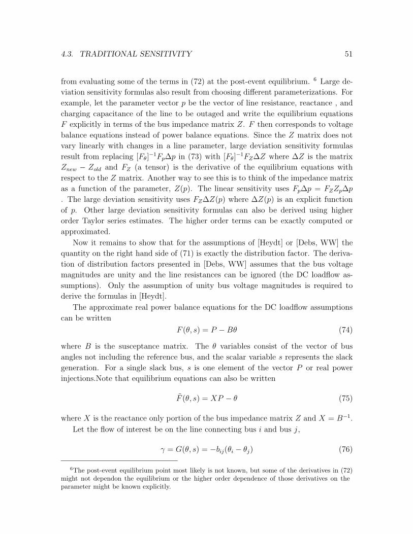
4.3. TRADITIONAL SENSITIVITY 51
from evaluating some of the terms in (72) at the post-event equilibrium. 6 Large de-
viation sensitivity formulas also result from choosing different parameterizations. For
example, let the parameter vector p be the vector of line resistance, reactance , and
charging capacitance of the line to be outaged and write the equilibrium equations
F explicitly in terms of the bus impedance matrix Z. F then corresponds to voltage
balance equations instead of power balance equations. Since the Z matrix does not
vary linearly with changes in a line parameter, large deviation sensitivity formulas
result from replacing [Fθ]−1Fp∆p in (73) with [Fθ]
−1FZ∆Z where ∆Z is the matrix
Znew − Zold and FZ (a tensor) is the derivative of the equilibrium equations with
respect to the Z matrix. Another way to see this is to think of the impedance matrix
as a function of the parameter, Z(p). The linear sensitivity uses Fp∆p = FZZp∆p
. The large deviation sensitivity uses FZ∆Z(p) where ∆Z(p) is an explicit function
of p. Other large deviation sensitivity formulas can also be derived using higher
order Taylor series estimates. The higher order terms can be exactly computed or
approximated.
Now it remains to show that for the assumptions of [Heydt] or [Debs, WW] the
quantity on the right hand side of (71) is exactly the distribution factor. The deriva-
tion of distribution factors presented in [Debs, WW] assumes that the bus voltage
magnitudes are unity and the line resistances can be ignored (the DC loadflow as-
sumptions). Only the assumption of unity bus voltage magnitudes is required to
derive the formulas in [Heydt].
The approximate real power balance equations for the DC loadflow assumptions
can be written
F (θ, s) = P − Bθ (74)
where B is the susceptance matrix. The θ variables consist of the vector of bus
angles not including the reference bus, and the scalar variable s represents the slack
generation. For a single slack bus, s is one element of the vector P or real power
injections. Note that equilibrium equations can also be written
F (θ, s) = XP − θ (75)
where X is the reactance only portion of the bus impedance matrix Z and X = B−1.
Let the flow of interest be on the line connecting bus i and bus j,
γ = G(θ, s) = −bij(θi − θj) (76)
6The post-event equilibrium point most likely is not known, but some of the derivatives in (72)might not depend on the equilibrium or the higher order dependence of those derivatives on theparameter might be known explicitly.

52 CHAPTER 4. SENSITIVITY COMPUTATIONS
Since the equilibrium equations are linear, Fθ is a constant complex matrix where
each column corresponding to a bus angle is exactly a column of the B matrix and
the single column corresponding to the slack generation is zero except for a one in
the row (assume the s row) corresponding to the slack power balance equation. Gθ is
a row vector of all zeros except in the columns corresponding to the buses connected
by the line, which contain the line susceptance; denote this vector b where
b = (0, ...,−bij, 0, ..., bij, 0, ..., 0) (77)
and bij = 1/xij. Assume that the parameter p is a complex power injection at bus k,
so that Gp is zero and Fp = e(k) is a column vector of all zeros except a one in the
k-th row corresponding to the bus injection. Equation (69) becomes
0 =
(B e(s) 0
b 0 −1
)
Θp
SpGp
+
(e(k)
0
)(78)
Equation (70) becomes
0 = w
(B e(s)
b 0
)(79)
If neither bus i or j is the slack bus, w = (bX,−1), and equation (71) becomes
Γp = −bXe(k) (80)
The b row vector “hits” only the i and j rows of X and the e(k) column vector “hits”
only the k-th column of X . Equation (80) can be written
Γp =Xik −Xjk
xij= ρij,k (81)
which is the commonly accepted formula for the distribution factors. Note that if
Equation (75) was used instead of Equation (74) to define the equilibrium condition
the same result is obtained. The steps follow in the same manner except that Fθ is
an identity matrix and Fp is the X matrix multiplied by e(k).
The [Heydt] assumption implies approximate complex equilibrium equations
0 = diag(θ∗)S∗ − Y ∗θ∗ (82)
where θ is complex and “diag” is the map of a vector to a diagonal matrix with
the vector entries in the same order on the diagonal. To get the distribution factor
formulas in [Heydt] simply use the full impedance and admittance matrices (replace
Y with B and Z with X using common notation). Equation (81) becomes
Γp =Zik − Zjk
zij= ρij,k (83)

4.4. PENALTY FACTORS, β COEFFICIENTS, AND NORMAL VECTORS 53
The estimates of line flows computed from these distribution factors are equivalent to
the updates of line flows resulting from one iteration of the fast decoupled loadflow.
Outage distribution factors are traditionally obtained by applying the distribution
factor formula for (complex) power injections that cancel the flow on the outaged line
(compensation). This corresponds to selecting p as a vector of power injections at the
connected buses and can also be derived by assuming that the parameter p represents
the outaged line parameter vector as in [GDA98]. Finally, large deviation sensitivity
formulas should be used for outage distribution factors. This is accomplished by
using the post outage Z bus (or X) bus quantities in the formula, which can be
computed from the Y bus (or B bus) changes using the matrix inversion lemma [Debs,
Bergen]. This is justified since the approximations yield linear models with constant
Jacobian matrices. For example, to derive the large sensitivity outage distribution
factors, replace the Θp∆p term from (73) with ∆Θ = P∆X . Note that different large
sensitivity outage distribution factors can be derived from the general formula (71)
without the fast decoupled loadflow assumptions.
4.4 Penalty factors, β coefficients, and normal vec-
tors
The effectiveness of each generator in a power system in servicing load depends upon
the location of that generator relative to the loads in the network. Due to transmission
losses, a generator that produces power inexpensively but is located a great distance
from loads might not be any more economical than an expensive generator located
close to major loads. The penalty factor associated with a generation bus indicates the
extent to which that generator is hindered by transmission losses. The β coefficients
are the reciprocals of the penalty factors. In this section we derive an expression
for the penalty factors and β coefficients based on the normal vector formula. The
formula is general and applies to many possible models of the power system.
If the cost to generate power at two buses is equal, then the bus with the higher
β (or lower penalty factor) will be most economical. Similarly, a load with a higher
β is more costly to service. In the recent jargon of the California ISO, the β coef-
ficients are referred to as “meter-multipliers”. The penalty factors and “betas” are
usually derived in power systems texts in a chapter concerning economic dispatch and
optimum power flow. The product of each generator’s β coefficient and incremental
cost is shown to be equal to the system Lagrange multiplier, referred to as “system
lambda”. In short, total cost is minimized when the product of each generator’s loss
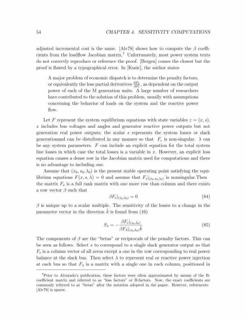
54 CHAPTER 4. SENSITIVITY COMPUTATIONS
adjusted incremental cost is the same. [Alv78] shows how to compute the β coeffi-
cients from the loadflow Jacobian matrix.7 Unfortunately, most power system texts
do not correctly reproduce or reference the proof. [Bergen] comes the closest but the
proof is flawed by a typographical error. In [Kusic], the author states
A major problem of economic dispatch is to determine the penalty factors,
or equivalently the loss partial derivatives ∂PL∂Pi
, as dependent on the output
power of each of the M generation units. A large number of researchers
have contributed to the solution of this problem, usually with assumptions
concerning the behavior of loads on the system and the reactive power
flow.
Let F represent the system equilibrium equations with state variables z = (x, s).
x includes bus voltages and angles and generator reactive power outputs but not
generation real power outputs; the scalar s represents the system losses or slack
generation and can be distributed in any manner so that Fz is non-singular. λ can
be any system parameters. F can include an explicit equation for the total system
line losses in which case the total losses is a variable in x. However, an explicit loss
equation causes a dense row in the Jacobian matrix used for computations and there
is no advantage to including one.
Assume that (x0, s0, λ0) is the present stable operating point satisfying the equi-
librium equations F (x, s, λ) = 0 and assume that Fz|(x0,s0,λ0) is nonsingular. Then
the matrix Fx is a full rank matrix with one more row than column and there exists
a row vector β such that
βFx|(z0,λ0) = 0 (84)
β is unique up to a scalar multiple. The sensitivity of the losses to a change in the
parameter vector in the direction k is found from (16)
Sλ = −βFs|(z0,λ0)
βFλ|(z0,λ0)k(85)
The components of β are the “betas” or reciprocals of the penalty factors. This can
be seen as follows. Select s to correspond to a single slack generator output so that
Fs is a column vector of all zeros except a one in the row corresponding to real power
balance at the slack bus. Then select λ to represent real or reactive power injection
at each bus so that Fλ is a matrix with a single one in each column, positioned in
7Prior to Alvarado’s publication, these factors were often approximated by means of the B-coefficient matrix and referred to as “loss factors” or B-factors. Now, the exact coefficients arecommonly referred to as “betas” after the notation adopted in the paper. However, reference to[Alv78] is sparse.

4.5. EXAMPLE: LINE OVERLOAD 55
the rows corresponding to real or reactive power balance at a bus. If k is a vector
with only one nonzero entry for load increase at one bus, Equation (85) computes
the sensitivity of the required power output of the slack bus with respect to increase
in demand at one bus. If there is one slack generator or marginal generator, it is
convenient to normalize β so that the component corresponding to that generator is
one.
Another interpretation is that the β vector determines the normal vector in pa-
rameter space to the surface on which the parameters must change to maintain an
equilibrium solution. Consider a formulation without a specific slack generator or
slack distribution. Let X(t) represent a curve in state space and Λ(t) a curve in
parameter space as functions of a scalar t so that
F (X(t),Λ(t)) = 0 (86)
Then the tangent vector (X, Λ) to the curve (X(t),Λ(t)) at (x0, λ0) satisfies
(Fx Fλ
)∣∣∣(x0,λ0)
(X
Λ
)= 0 (87)
Pre-multiply (87) by β to obtain the normal vector, N to Λ(t) at λ0 is
N = βFλ|(x0,λ0) (88)
where β is found from (84).
The concept of penalty factors has been generalized. By appropriate choice of the
vector λ the penalty factor or “beta” corresponding to real or reactive power injection
at any bus can be computed. However, there is no reason to limit the parameters
to bus injections or the equations to the standard loadflow equations. For example,
if interchange equations are appended with additional variables to maintain the set
interchanges, the penalty factor associated with each interchange can be computed
and thus the value of power at each interchange. This allows the optimum interchange
set points to be determined within the economic dispatch solution. In addition, linear
and quadratic estimates of the changes in losses resulting from interarea transactions
could be computed efficiently.
4.5 Example: line overload
We conclude this chapter with a simple illustration that uses the sensitivity formulas.
Assume that the critical event located by the continuation program for the forecast
parameter change was a line overload. It is desired to move away from the overload
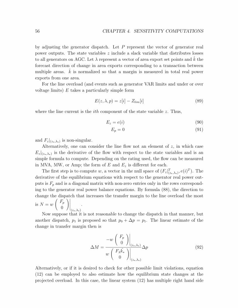
56 CHAPTER 4. SENSITIVITY COMPUTATIONS
by adjusting the generator dispatch. Let P represent the vector of generator real
power outputs. The state variables z include a slack variable that distributes losses
to all generators on AGC. Let λ represent a vector of area export set points and k the
forecast direction of change in area exports corresponding to a transaction between
multiple areas. k is normalized so that a margin is measured in total real power
exports from one area.
For the line overload (and events such as generator VAR limits and under or over
voltage limits) E takes a particularly simple form
E(z, λ, p) = z[i]− Zlim[i] (89)
where the line current is the ith component of the state variable z. Thus,
Ez = e(i) (90)
Ep = 0 (91)
and Fz|(z∗,λ∗) is non-singular.
Alternatively, one can consider the line flow not an element of z, in which case
Ez|(z∗,λ∗) is the derivative of the flow with respect to the state variables and is an
simple formula to compute. Depending on the rating used, the flow can be measured
in MVA, MW, or Amp; the form of E and Ez is different for each.
The first step is to compute w, a vector in the null space of (Fz|T(z∗,λ∗), e(i)T ). The
derivative of the equilibrium equations with respect to the generator real power out-
puts is Fp and is a diagonal matrix with non-zero entries only in the rows correspond-
ing to the generator real power balance equations. By formula (88), the direction to
change the dispatch that increases the transfer margin to the line overload the most
is N = w
(Fp0
)∣∣∣∣∣(z∗,λ∗)
.
Now suppose that it is not reasonable to change the dispatch in that manner, but
another dispatch, p1 is proposed so that p0 + ∆p = p1. The linear estimate of the
change in transfer margin then is
∆M =
−w(Fp0
)∣∣∣∣∣(z∗,λ∗)
w
(Fλk∗
0
)∣∣∣∣∣(z∗,λ∗)
∆p (92)
Alternatively, or if it is desired to check for other possible limit violations, equation
(12) can be employed to also estimate how the equilibrium state changes at the
projected overload. In this case, the linear system (12) has multiple right hand side

4.5. EXAMPLE: LINE OVERLOAD 57
since Fp is a matrix so it is best to parameterize p by a scalar t so that (12) is
computed using the vector right hand side Fpp, yielding Z so that ∆Z = Z∆t where
∆p = Fpp∆t.
Finally, the most economical direction to dispatch generation and not cause over-
load can be found by solving a linear program minimizing the cost of generation
subject to the constraint that equilibrium is met and the line rating is not exceeded.
If Θ(p) is the generator cost function, and β the reciprocals of the penalty factors,
the linear program minimizes Θp∆p subject to the constraints that
β∆p = 0 (93)
and
N∆p ≤ 0 (94)
The next two chapters detail the case where the critical event is a fold bifurcation
of the equilibrium equations.

58
59
Chapter 5
Margin and Sensitivity Methods
for Voltage Collapse
This chapter concerns computing and exploiting the sensitivity of the loading margin
to voltage collapse with respect to various parameters. The main idea of this chapter
is that after the loading margin has been computed for nominal parameters, the effect
on the loading margin of altering the parameters can be predicted by Taylor series
estimates. [GDA97] is a concise version of this chapter.
Loading margin is a fundamental measure of proximity to voltage collapse. Linear
and quadratic estimates to the variation of the loading margin with respect to any
system parameter or control are derived. Tests with a 118 bus system indicate that the
estimates accurately predict the quantitative effect on the loading margin of altering
the system loading, reactive power support, wheeling, load model parameters, line
susceptance, and generator dispatch. The accuracy of the estimates over a useful
range and the ease of obtaining the linear estimate suggest that this method will be
of practical value in avoiding voltage collapse.
5.1 Introduction
Voltage collapse is an instability of heavily loaded electric power systems characterized
by monotonically decreasing voltages and blackout [DCL, Davos]. Secure operation
of a power system requires appropriate planning and control actions to avoid voltage
collapse. This chapter describes and illustrates the use of loading margin sensitivities
for the avoidance of voltage collapse.
For a particular operating point, the amount of additional load in a specific pattern
of load increase that would cause a voltage collapse is called the loading margin.
We are interested in how the loading margin of a power system changes as system
parameters or controls are altered. This chapter describes how to compute linear
and quadratic Taylor series estimates for the variation of the loading margin with
respect to any power system parameter or control. The effects on the loading margin
of changing the following controls and parameters is estimated:

60 CHAPTER 5. VOLTAGE COLLAPSE
• Emergency load shedding
• Reactive power support, shunt capacitance
• Variation in the direction of load increase
• Interarea redispatch, wheeling
• Changes to load model and load composition
• Varying line susceptance, FACTS device
• Generator redispatch
Loading margin sensitivities have a simple geometric meaning. Figure 6 shows
nose curves of a large power system for three values of a power system parameter.
The loading margin is the change in loading between the stable operating point and
the nose of the curve corresponding to each parameter setting. The nose corresponds
to a saddle-node bifurcation point of the power system when it is parameterized by
loading, and is often referred to as the “point of collapse” or “bifurcation point”.
A similar set of curves results for varying any other system parameter, such as the
line impedance or powerfactor of the load. As the parameter increases, the nose
of the curve occurs at a higher loading and the loading margin increases. Figure 7
shows the loading margin as a function of the parameter value. Each nose curve in
Figure 6 contributes one point to Figure 7. The sensitivity of the loading margin
with respect to the parameter at the nominal parameter value is given by the tangent
linear approximation to the curve in Figure 7. Once the loading margin has been
computed for nominal parameters, the effect on the loading margin of altering the
parameters can be predicted by using linear or quadratic estimates. Exhaustively
recomputing the nose for each parameter change is avoided.
Loading margin is an accurate measure of proximity to voltage collapse which takes
full account of system limits and nonlinearities. Moreover, loading margin estimates
can be directly associated with costs, allowing for economic comparison of different
strategies [Alv91]. Methods to compute the nose and hence the loading margin are
presented in [CA93, CFSB, AC92, VC91, Iba] and are discussed in Chapter 2.
Another approach to assessing proximity to voltage collapse uses fast time-domain
simulation to predict whether the system will collapse (e.g. [Kur93, DS93]). This
approach has the advantage of better representing the potentially complex series
of time dependent events which can influence voltage collapse. For example, the
time dependence of generator reactive power limits can be represented. However,
sensitivity information is difficult to obtain from time-domain simulations and requires
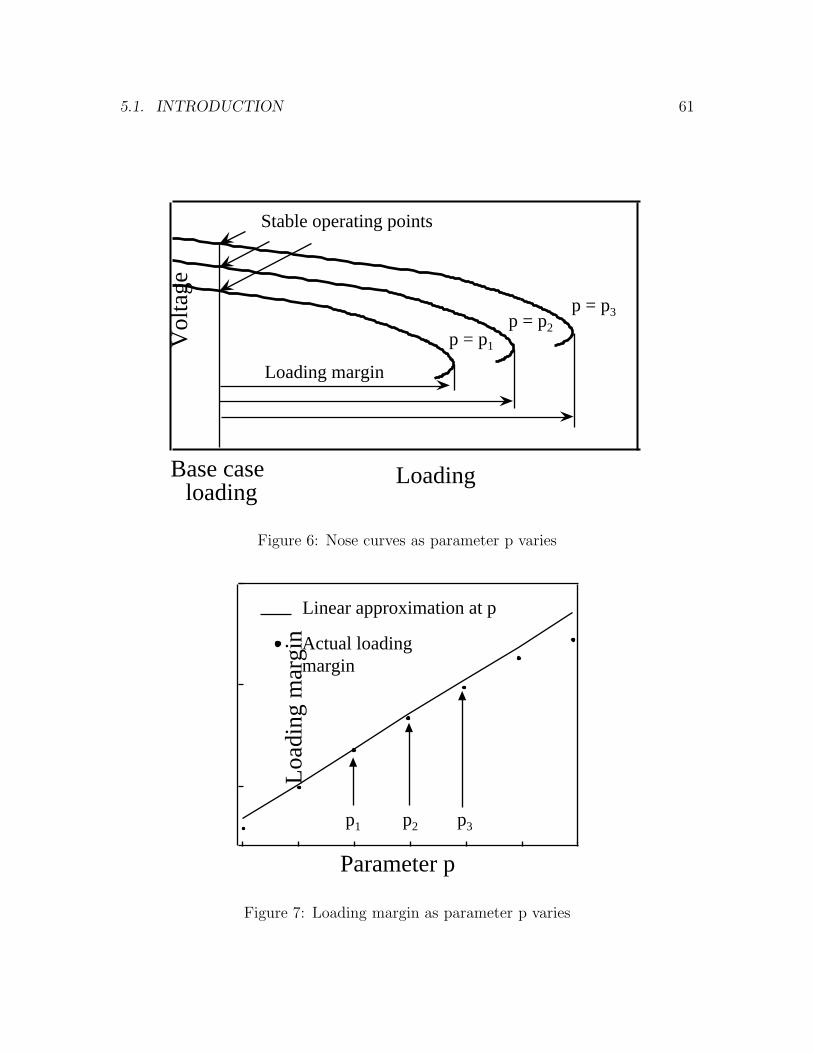
5.1. INTRODUCTION 61
Vol
tage
Loading
p = p1
Loading margin
Stable operating points
Base caseloading
p = p2
p = p3
Figure 6: Nose curves as parameter p varies
Linear approximation at p
Actual loading margin
Loa
ding
mar
gin
Parameter p
p2 p3p1
Figure 7: Loading margin as parameter p varies

62 CHAPTER 5. VOLTAGE COLLAPSE
a new simulation for each parameter variation considered. A single computation of
a loading margin uses a power system model with some approximations but can
yield a wealth of useful sensitivity information. The loading margin and time-domain
simulation approaches are complementary. Recent work combines aspects of both
approaches [VC94].
There has been previous work on the sensitivity of various indices for voltage
collapse. Tiranuchit and Thomas [TT88] computed the sensitivity of the minimum
singular value of the system Jacobian and Overbye and DeMarco [OD91] computed
the sensitivity of an energy function index. The first order sensitivity of the loading
margin was derived by Dobson and Lu [DL192]. This chapter is an extension and
application of [DL192].
In a discussion to [GDA97], Wu, Fischl, and Nwankpa reference [WF93] which uses
an optimization formulation (or regularization method) to derive sensitivity formulas
similar to those here and in [GDA97]. The first order sensitivity formula of [WF93]
can be shown to be equivalent to the first order sensitivity formula derived in this
report and in [GDA97]. However, the second order sensitivity formula of [WF93]
does not agree with the second order sensitivity formula of [GDA97] and this report.
The reason for the discrepancy is an error in the derivation of [WF93]. Wu, Fischl,
and Nwankpa raise several topics motivating the work in Chapter 6 and [GDA98].
The complete discussion and closure to [GDA97] appears in the IEEE Transactions
[GDA97].
5.2 Theoretical background and assumptions
One influential theory of voltage collapse [DC89] models the power system as differ-
ential equations with slowly moving parameters and describes voltage collapse as the
dynamic consequence of a saddle node bifurcation. In a saddle node bifurcation, the
stable operating equilibrium coalesces with an unstable equilibrium and disappears.
The dynamic consequence of a generic saddle node bifurcation is a monotonic decline
in system variables.
Although differential equations are the proper setting for understanding voltage
collapse and are necessary for explaining why voltages dynamically decrease as a
consequence of a saddle node bifurcation, it is possible and very advantageous to
compute loading margins to voltage collapse and their sensitivities using static equa-
tions [Dob94]. These static equations are equivalent to equations derived from the
differential equations by setting all the derivatives to zero. Usually the exact dynamic
equations of the power system are poorly known. For example, both the form and
data for dynamic load models for voltage collapse studies are controversial. However,
5.3. INFORMAL DERIVATION 63
static models of the power system are much better known. The idea is to use the
static models for computations, while supposing there to be underlying dynamics of
a sensible form whose equilibrium equations reduce to the static models. Dobson
[Dob94] proves that there is no loss of accuracy in using static models in place of the
underlying dynamic models when computing loading margins and their sensitivities.
The derivations and application of the sensitivity formulas require the choice of
a nominal stable operating point at which parameters or controls are to be adjusted,
and a projected pattern of load increase. The pattern of load increase determines the
nominal bifurcation point (nose) and also defines the direction in which the loading
margin is measured. The bifurcation point should be computed by a method that
takes into account system limits such as generator reactive power limits as they are
encountered. In general, the limits enforced at the bifurcation are different than those
at the stable operating point. The derivation of the sensitivity formulas requires that
the system equations remain the same as parameters are varied. In particular, the
limits enforced at the bifurcation are assumed to stay the same as parameters are
varied.
5.3 Informal derivation
This section informally derives the first order sensitivity of the loading margin L with
respect to any parameter p. See Chapter 4 and the appendices of this chapter for a
rigorous derivation of this and the quadratic sensitivity formulas.
Suppose that the equilibria of the power system satisfy the equations
f(x, λ, p) = 0 (95)
where x is the vector of state variables and λ is the vector of real and reactive load
powers. Let λ0 be the real and reactive powers at the operating equilibrium. We
specify a pattern of load increase with a unit vector k. Then the load powers at the
saddle node bifurcation causing voltage collapse are
λ = λ0 + kL (96)
where L is the loading margin. The choice of norm is arbitrary, k is a unit vector in
whatever norm is used to measure the loading margin L. Since k is a unit vector, it
also follows that L = |λ− λ0|.At a saddle node bifurcation, the Jacobian matrix fx is singular. For each (x, λ, p)
corresponding to a bifurcation, there is a left eigenvector w(x, λ, p) (a row vector)
corresponding to the zero eigenvalue of fx such that
w(x, λ, p)fx(x, λ, p) = 0 (97)

64 CHAPTER 5. VOLTAGE COLLAPSE
The points (x, λ, p) satisfying (95) and (97) correspond to bifurcations and a curve of
such points can be obtained by varying p about its nominal value p∗. Linearization
of this curve about the bifurcation (x∗, λ∗, p∗) yields
fx|∗∆x + fλ|∗∆λ + fp|∗∆p = 0 (98)
where fλ is the derivative of f with respect to the load powers λ and fp is the
derivative of f with respect to the parameter p. ‘|∗’ means ‘evaluated at (x∗, λ∗, p∗)’.
Pre-multiplication by w = w(x∗, λ∗, p∗) yields
wfλ|∗∆λ + wfp|∗∆p = 0 (99)
since (97) implies that wfx|∗ = 0. Equation (99) can be interpreted as stating that
(wfλ|∗, wfp|∗) is the normal vector at (λ∗, p∗) to the bifurcation set in a load power
and parameter space [DL192].
Using the parameterization of λ by L from (96) yields ∆λ = k∆L and substitution
in (99) gives
wfλk∆L+ wfp ∆p = 0 (100)
and hence the sensitivity of the loading margin to the change in parameters is
Lp|∗ =−wfp|∗wfλ|∗ k
(101)
For the linear estimate we use (101) and
∆L = Lp|∗∆p (102)
The same formula holds for multiple parameters p, in which case wfp|∗ is a vector
(see appendices). This is useful when approximating the combined effects of changes
in several parameters or when comparing the effects of various parameters on the
loading margin.
For the quadratic approximation we use (101), (113) and
∆L = Lp|∗∆p+1
2Lpp|∗(∆p)2 (103)
5.4 Application to test system
The practical use of the sensitivity formulas derived in the previous section and the
appendices is illustrated using a particular voltage collapse of the 118 bus IEEE
standard test system [wahoo]. (Refer to [wahoo] to reproduce the results. Also area

5.4. APPLICATION TO TEST SYSTEM 65
numbers and bus numbers correspond to those in [wahoo].) The system loading and
loading margin is measured by the sum of all real load powers (an L1 norm). The
stable operating point at which we test parameter variation has a total system loading
of 5677 MW. Buses critical to the voltage collapse are in area two. The generator
dispatch distributes the slack so that generators in each area provide additional real
power roughly in proportion to their size. The loads increase proportionally from the
base case loading and the voltage collapse occurs for a total load of 7443 MW and a
loading margin of 1766 MW. Seven generators reach reactive power limits between the
stable operating point and the voltage collapse. (Note that the reactive power limit
for generator 4 is increased to avoid complications caused by an immediate instability
that would have occurred just prior to the voltage collapse. An immediate instability
[DL292] can be caused by a generator reaching a reactive power limit.)
The sensitivity formulas evaluated at the voltage collapse yield linear and quadratic
estimates of the loading margin as a function of any parameter. The performance of
these estimates is tested for seven different parameters representative of a range of
control actions or system uncertainties. The solid lines and dotted curves in Figures
8 thru 14 are the respective linear and quadratic estimates for the loading margin
variation as a function of the chosen parameter.
The dots in Figures 8 thru 14 represent the actual values of the loading margin
as computed by combined continuation and direct methods [CA93]. The large dots
represent the loading margin computed assuming that the reactive power limits which
apply at the voltage collapse remain the same when the parameters are varied. (This
assumption was used in deriving our sensitivity formulas.) The small dots represent
the actual loading margin allowing different reactive power limits to apply at the
voltage collapse. The small dots are computed by enforcing generator reactive power
limits as the loading is increased from the stable operating point.
Both the small and large dots take into account limits as the loading is increased
from the base case, but changes in the limits due to parameter variations are only
accounted for by the small dots. The small dots test the practicality of using the
estimates in a setting where the limits can vary. In Figures 8 thru 13, the assumptions
about limits make little difference and the large dots cover the small dots. The effects
of limits will be addressed as future work in later chapters.
5.4.1 Emergency load shedding
Bus 3 is a strong candidate for load shedding based on the magnitude of the compo-
nents of the left zero eigenvector at the bifurcation. At the stable operating point, bus
3 has a load of 60 MW and 15 MVARs and a voltage of .95 p.u. Figure 8 shows the
results for shedding up to 60 MW of base load at constant power factor. Each MW

66 CHAPTER 5. VOLTAGE COLLAPSE
1800
1900
2000
0 10 20 30 40 50 60
LinearActual
Loa
ding
mar
gin
(MW
)
Load reduction (MW)
Figure 8: Effect of load shedding on voltage collapse margin
of load reduction increases the loading margin by 3.5 MW, and the relation remains
almost linear over the entire range of load shed.
Note that “load shedding” could refer to several distinct situations requiring dif-
ferent use of the Taylor series formulas. For the example shown here, we shed a
specific amount of real and reactive power at the base loading at one bus. However,
the load at that bus still increases from the base case at the same power factor and at
the same rate as assumed for the nominal case. If one wishes instead to estimate the
effect of shedding base load and not increasing the load at this bus, then one must
account for changes to all the system parameters effected. Specifically, the change in
the direction of load increase k , and the change in base load must both be accounted
for. An example of changing the direction of load increase follows.

5.4. APPLICATION TO TEST SYSTEM 67
5.4.2 Direction of load increase
Computing the loading margin requires a direction of load increase to be assumed.
Variation in the direction of load increase can result from temperature dependence of
the loads or inaccuracies in forecasting. Thus it is useful to estimate the sensitivity
of the loading margin to the direction of load increase.
The direction of load increase is multi-dimensional, so that not every conceivable
variation can be parameterized in such a way that a 2-dimensional graph is compre-
hensible. To ease visualization, we choose to parameterize the change in direction
by a scalar. For this example, the direction of load increase is varied by transferring
load increase from the critical bus 1 to a less critical bus in the same area, bus 23.
For a particular loading factor, the total load remains the same but the proportion of
load at bus 23 increases and the proportion at bus 1 decreases. Figure 9 shows that a
linear estimate for the change in the loading margin performs well over the full range
of variation.
5.4.3 Reactive power support
The largest generator in area two is at bus 10, which is connected by a long transmis-
sion line to the high voltage side of the network. At the stable operating point, the
generator at bus 10 is near its reactive power limit. Bus 9 represents the midpoint of
the transmission line, and is a logical place to consider adding reactive power to alle-
viate the voltage collapse. The addition of shunt capacitance at bus 9 could represent
operation of switched capacitors or SVC. Figure 10 shows that the linear estimate is
accurate and quantifies the effectiveness of reactive power support at bus 9.
5.4.4 Area interchange
Recent trends in deregulation are expected to increase wheeling which can affect
system security.
Figure 11 shows the effects on the loading margin of adjusting the flows between
area 2 and the main area. The nominal interchange between the main area and area 2
is 103 MW. Importing an additional 100 MW results in an increase in loading margin
of over 200 MW, which is well predicted by the linear estimate.
The adjustment of the interarea flows caused the number of generators reaching
reactive power limits to change, yet these changes did not significantly affect the
accuracy of the estimates. Most of the additional generators that reached limits were
not at critical buses. The linear estimates were accurate for varying the interarea
flow by plus or minus 100 percent.

68 CHAPTER 5. VOLTAGE COLLAPSE
1760
1770
1780
1790
1800
0 0.2 0.4 0.6 0.8 1
Linear
Actual
Loa
ding
mar
gin
(MW
)
Proportion of load increase transferred from bus 1 to bus 23
Figure 9: Effect of assumed loading direction on voltage collapse margin

5.4. APPLICATION TO TEST SYSTEM 69
1800
1900
2000
0 0.1 0.2 0.3 0.4
Linear
Actual
Loa
ding
mar
gin
(MW
)
Shunt capacitance (p.u.)
Figure 10: Effect of shunt capacitance on voltage collapse margin
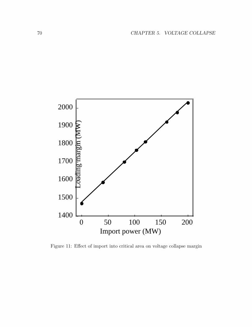
70 CHAPTER 5. VOLTAGE COLLAPSE
1400
1500
1600
1700
1800
1900
2000
0 50 100 150 200
Loa
ding
mar
gin
(MW
)
Import power (MW)
Figure 11: Effect of import into critical area on voltage collapse margin

5.4. APPLICATION TO TEST SYSTEM 71
5.4.5 Load model
Load models are important in voltage collapse studies. The sensitivity of the loading
margin with respect to parameters of a load model can be used to estimate the effect
on the loading margin of using more detailed models. Figure 12 shows the effect on
the loading margin of an additional reactive load Q at bus 3 linearly dependent upon
the bus voltage V so that Q = KV . K can be interpreted as MVARS at 1 p.u.
voltage.
For this case we add voltage dependent load at bus 3, we do not change the con-
stant power factor base load or change the rate of constant power factor load increase.
If instead we were to assume that the original base load was voltage dependent, then
a different computation would be performed taking account changes to all the pa-
rameters affected. In addition, one must specify how the direction of load increase
and the loading margin measure are affected by any parameter changes. It is cer-
tainly possible to have either or both the direction of load increase or the measure
of the loading margin dependent upon some load model parameters. The formulas
presented in this chapter are general and can be applied to these cases, but care must
be taken in computing the derivatives and applying the chain rule correctly.
5.4.6 Line susceptance
Variations in a line susceptance could represent the operation of a FACTS device or
could reflect uncertainty in the network data. Figure 13 shows the effect of altering
the susceptance of the line connecting bus 9 to bus 10.
For this example, the quadratic estimate is required to obtain accurate results
over the full range of variation and the effects of changing limits are noticeable but
not significant.
5.4.7 Generator dispatch
Generators 10 and 12 together assume 50% of the slack for area 2 with generator 10
alone picking up 42% for the nominal dispatch. Figure 14 shows the effect of shifting
slack from generator 10 to generator 12. The two generators participate equally in the
dispatch when 17% of the total area slack is moved from generator 10 to generator 12.
Figure 14 shows that the distribution of real power can greatly affect the loading
margin and that the quadratic estimate is accurate over a much larger range than
the linear estimate. Moreover, the effects of limits can be significant. In this case,
shifting more than 15% of the total area slack to generator 12 prevents generator 10
from reaching its reactive power limit; additional transfer past this point has little

72 CHAPTER 5. VOLTAGE COLLAPSE
1650
1700
1750
1800
0 10 20 30 40 50 60 70 80 90 100
Loa
ding
mar
gin
(MW
)
K
Linear
Quadratic
Actual
Figure 12: Effect of composition of load model on voltage collapse margin

5.4. APPLICATION TO TEST SYSTEM 73
1200
1400
1600
1800
2000
2200
2400
2600
16 24 32 40 48
Linear
Quadratic
Actual, same limits
Actual, different limits
Loa
ding
mar
gin
(MW
)
Susceptance (p.u.)
Figure 13: Effect of susceptance on voltage collapse margin

74 CHAPTER 5. VOLTAGE COLLAPSE
effect on the loading margin.
5.5 Discussion
The loading margin sensitivities only depend on quantities evaluated at the nominal
bifurcation point. Evaluation of the linear sensitivity is particularly simple. Once the
nominal bifurcation point is computed, the linear sensitivity requires computation
of the left eigenvector w and the derivative fp|∗ of the power system equations with
respect to the parameter. In many cases fp|∗ has only one or two nonzero entries. w
can be found by inverse power methods or as a byproduct of a direct method used
to refine location of the bifurcation point [DL192]. Since w is the same regardless of
the parameter chosen, it is very quick to compute the sensitivity to any additional
parameters.
The quadratic estimate additionally requires solution of a sparse set of linear
equations (109,111), the right eigenvector v and some second order derivatives. The
second order derivatives include the matrix wfxx|∗, where fxx|∗ is the Hessian tensor.
wfxx|∗ can be obtained as a byproduct of a direct method that uses a Newton iteration.
The other higher order derivatives are more easily obtained and often evaluate to zero.
When the quadratic term is small, it increases confidence in the accuracy of the linear
estimate. When the quadratic term is not small, it serves as a more accurate estimate.
One source of inaccuracy is the neglect of higher order terms in the estimates.
When the computed bifurcation is near a different bifurcation corresponding to volt-
age collapse of another area of the system, movement of the parameter can cause the
voltage collapse to ‘shift’ from one area to the other. Since the set of critical pa-
rameters and loadings could have significant variations in curvature in this case, the
linear and quadratic estimates would be useful only over a small parameter range.
(The area of the power system corresponding to a bifurcation is described by the
right eigenvector v corresponding to the Jacobian singularity since the components of
v specify the relative participation of bus voltages and angles in the voltage collapse
[DC89, Dob92].)
Another source of inaccuracy is that the estimates assume a fixed set of equations
whereas the form of the equations can change discretely whenever a parameter varia-
tion causes power system limits to change. The 118 bus system results are examples
in which this does not significantly impair the usefulness of the estimates. However,
this source of inaccuracy has the potential to be significant and requires awareness
when using the estimates. Future work could address the effect of limits on loading
margin sensitivities, perhaps by representing the effect of the limits using homotopy
methods [GreMS].

5.5. DISCUSSION 75
1800
2000
2200
2400
2600
2800
0 2 4 6 8 10 12 14 16
Loa
ding
mar
gin
(MW
)
Percentage of area slack shifted fromgenerator 10 to generator 12 (%)
Linear
Quadratic
Actual, same limits
Actual, different limits
Figure 14: Effect of generator dispatch on voltage collapse margin

76 CHAPTER 5. VOLTAGE COLLAPSE
The loading margin and sensitivity computations require only static power systems
equations but accurately reflect the proximity to voltage collapse of the dynamic
power system. In particular, explicit knowledge of load dynamics is not needed.
5.6 Conclusions
In this chapter linear and quadratic Taylor series estimates for the variation of the
loading margin with respect to any power system parameter or control are presented.
These estimates can be used to quickly assess the quantitative effectiveness of various
control actions to maintain a sufficient loading margin to voltage collapse. That is, the
computations approximate the change in loading margin for a given change in each
control. The estimates are also useful in determining the sensitivity of the loading
margin to uncertainties in data. Evaluation of the estimates is efficient; calculation
of any number of estimates requires only computation of a single nose or bifurcation
point of the power system.
The sensitivity formulas are more rigorously derived in the following appendix.
The quadratic estimate is new and the derivation of the linear estimate improves
on previous work in [DL192]. The derivation is independent of the norm chosen to
measure the loading margin.
The practical use of the sensitivity computations is illustrated for a range of system
parameters on a voltage collapse of the IEEE 118 bus system. The likely sources
of inaccuracy discussed in the previous section include variations in the generator
reactive power limits enforced at the nose. The results suggest that the linear estimate
is good for many parameters and can sometimes be improved with the quadratic
estimate. Direct comparison of different control actions can be made in terms of their
effect on the loading margin. The closeness of the estimates over a useful range of
parameter variations and the ease of obtaining the linear estimate suggest that the
sensitivity computations will be of practical value in avoiding voltage collapse.

5.7. APPENDICES 77
5.7 Appendices
Appendix 5.7.A Derivation of sensitivity formulas
Let f : IRn × IRm × IRl → IRn be a smooth function such that the solutions of
0 = f(x, λ, p) (104)
are the equilibria of the power system near (x∗, λ∗, p∗). We assume that f has a fold
bifurcation at (x∗, λ∗, p∗) satisfying:
F(a) f(x∗, λ∗, p∗) = 0
F(b) fx|∗ has rank n− 1
F(c) wfλ|∗ k 6= 0
F(d) wfxx|∗(v, v) 6= 0, where v and w are nonzero
vectors satisfying fx|∗v = 0 and wfx|∗ = 0.
These are the generic conditions for a fold bifurcation [CH]. (They differ slightly
from the conditions for a saddle node bifurcation and the distinction between the two
bifurcations is discussed in [Dob94]. The fold bifurcation is more appropriate when
working with static equations.)
Let λ0 be the base case loading and let the unit vector k ∈ IRm be a given direction
in loading space. The loading is parameterized by ` ∈ IR:
λ(`, k, λ0) = λ0 + ` k (105)
The loading may be measured with any norm, but different norms lead to different
unit vectors k. Let
g(x, `, p) = f(x, λ0 + `k, p) (106)
Since gx = fx, gxx = fxx, and g` = fλk, g also has a fold bifurcation at (x∗, `∗, p∗) and
the corresponding conditions F(a)-(d) are satisfied with g written for f except that
F(c) becomes wg`|∗ 6= 0.
Appendix 5.7.B proves that near (x∗, `∗, p∗) there is a smooth surface Ψ param-
eterized by p so that each point on Ψ corresponds to a fold bifurcation. Points on
Ψ are of the form (X(p), L(p), p) where X(p) defines the variation of the bifurcating
equilibrium with parameter p and L(p) defines the variation of the loading margin
with parameter p. In the useful case of one dimensional p, Ψ is a curve. Points of Ψ
satisfy
g(X(p), L(p), p) = 0 (107)
µ(X(p), L(p), p) = 0 (108)
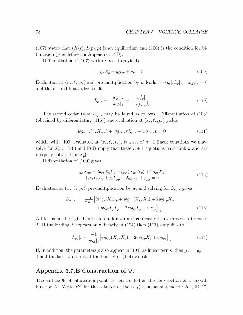
78 CHAPTER 5. VOLTAGE COLLAPSE
(107) states that (X(p), L(p), p) is an equilibrium and (108) is the condition for bi-
furcation (µ is defined in Appendix 5.7.B).
Differentiation of (107) with respect to p yields
gxXp + g`Lp + gp = 0 (109)
Evaluation at (x∗, `∗, p∗) and pre-multiplication by w leads to wg`|∗Lp|∗ + wgp|∗ = 0
and the desired first order result
Lp|∗ = −wgp|∗wg`|∗
= − wfp|∗wfλ|∗ k
(110)
The second order term Lpp|∗ may be found as follows. Differentiation of (108)
(obtained by differentiating (116)) and evaluation at (x∗, `∗, p∗) yields
wgxx|∗(v,Xp|∗) + wgx`|∗vLp|∗ + wgxp|∗v = 0 (111)
which, with (109) evaluated at (x∗, `∗, p∗), is a set of n + 1 linear equations we may
solve for Xp|∗. F(b) and F(d) imply that these n + 1 equations have rank n and are
uniquely solvable for Xp|∗.Differentiation of (109) gives
gxXpp + 2gx`XpLp + gxx(Xp, Xp) + 2gxpXp
+g``LpLp + g`Lpp + 2g`pLp + gpp = 0(112)
Evaluation at (x∗, `∗, p∗), pre-multiplication by w, and solving for Lpp|∗ gives
Lpp|∗ = −1wg`|∗
[2wgx`XpLp + wgxx(Xp, Xp) + 2wgxpXp
+wg``LpLp + 2wg`pLp + wgpp]∣∣∣∗
(113)
All terms on the right hand side are known and can easily be expressed in terms of
f . If the loading λ appears only linearly in (104) then (113) simplifies to
Lpp|∗ =−1
wg`|∗
[wgxx(Xp, Xp) + 2wgxpXp + wgpp
]∣∣∣∗
(114)
If, in addition, the parameters p also appear in (104) as linear terms, then gxp = gpp =
0 and the last two terms of the bracket in (114) vanish.
Appendix 5.7.B Construction of Ψ.
The surface Ψ of bifurcation points is constructed as the zero section of a smooth
function U . Write Bij for the cofactor of the (i, j) element of a matrix B ∈ IRn×n.
5.7. APPENDICES 79
Since condition F(b) states that gx|∗ has rank n − 1, we can find i and j such that
(gx|∗)ij 6= 0. Since the cofactors of a matrix are smooth functions of the entries of the
matrix, there is a neighborhood S ⊂ IRn×n of gx|∗ such that Bij 6= 0 for B ∈ S. De-
fine the smooth functions w(B) = (B1j, B2j , ..., Bnj) and v(B) = (Bi1, Bi2, ..., Bin)T .
Then
w(B)B = detB eTj and Bv(B) = detB ei (115)
where ei is a column vector of all zeros except that the ith position has value one.
w(B) and v(B) are non-zero vectors for B ∈ S. Define w = w(gx|∗) and v = v(gx|∗).It follows from (115) and det gx|∗ = 0 that w gx|∗ = 0 and gx|∗ v = 0 so that w and v
are nonzero vectors satisfying the conditions in the definition of the fold bifurcation.
Define the smooth map β : S → IR by β(B) = w(B)B v(B) It follows from (115)
that β(B) = BijdetB. Since gx is smooth, there is a neighborhood N about (x∗, `∗, p∗)
such that (x, `, p) ∈ N implies gx|(x,`,p) ∈ S. Define µ : N → IR by
µ(x, `, p) = β(gx(x, `, p))
= w(gx(x, `, p))gx(x, `, p)v(gx(x, `, p))(116)
and define U : N → IRn × IR by U(x, `, p) =
(g(x, `, p)
µ(x, `, p)
). Then Ψ is defined as the
zero section of U : Ψ = U−1(0).
The matrix (Ux, U`)|∗ =
(gx|∗ g`|∗
wgxx|∗v wgx`|∗v
)is invertible if a = b = 0 is the
only solution to (Ux, U`)|∗(a
b
)= 0, or, equivalently,
gx|∗a + g`|∗b = 0 (117)
wgxx|∗va+ wgx`|∗vb = 0 (118)
Since F(c) implies that g`|∗ is not in the range of gx|∗, to satisfy (117), b = 0 and
then F(b) implies that a = αv for some scalar α. Then (118) with b = 0 yields
αwgxx|∗(v, v) = 0 and F(d) implies α = 0 and a = 0. Thus (Ux, U`)|∗ is invertible.
It then follows from the implicit function theorem that there is a neighborhood P
of p∗ and smooth functions X : P → IRn and L : P → IR such that {(X(p), L(p), p) |p ∈ P} ⊂ Ψ and U(X(p), L(p), p) = 0, which can be rewritten as (107) and (108).
Appendix 5.7.C Sensitivity of the margin to the locally closest
fold bifurcation.
In the discussion to [GDA97], Canizares inquires about sensitivity of the margin when
we do not assume a particular direction of load increase but instead allow the direction

80 CHAPTER 5. VOLTAGE COLLAPSE
of load increase to vary. For example, one maybe interested in the sensitivity of the
margin to a locally closest bifurcation [Dob93], and thus k would not be a constant
but must vary to satisfy the conditions of a locally closest bifurcation. Similarly, the
example given in this chapter for changing the direction of load increase requires that
k be considered as a function of the parameter being varied. Specifically, equation
(106) could be written
g(x, `, p) = f(x, λ0 + `k(p), p) (119)
to emphasize the dependence of k on p. Equation (110) then becomes
Lp|∗ = −wgp|∗ + wg`|∗kpL0
wg`|∗= −
wfp|∗ + wfλ|∗kpL0
wfλ|∗k(120)
Now we consider the case of the sensitivity of the margin to the locally closest
bifurcation. In this case L0 is the margin from the base loading to the nominal closest
bifurcation in the direction k. At a locally closest bifurcation,
wfλ|∗ −∣∣∣∣wfλ|∗
∣∣∣∣kT = 0 (121)
where |wfλ|∗| is the norm of wfλ|∗. Substituting for wfλ|∗ in the numerator of (120)
yields
Lp|∗ = −wfp|∗ +
∣∣∣∣wfλ|∗∣∣∣∣kTkpL0
wfλ|∗k(122)
In general, to find kp one must specify the norm for k as well as the normalization
of the eigenvectors. However, for the common case where k is a unit vector in an L2
norm, kTkp = 0 and (122) reduces to
Lp|∗ = − wfp|∗wfλ|∗k
(123)
which is exactly the first order sensitivity formula used for the less general param-
eterizations of λ. This result is also obtained in [Dob93]. The derivation of higher
order terms can also be generalized for the case where k changes to identify a locally
closest bifurcation. However, the formulas will be dependent upon the normalizations
assumed and can additionally require computation of the eigenvector sensitivities.

Chapter 6
Contingency Analysis for Voltage
Collapse
This chapter presents a contingency ranking method for voltage collapse. The change
in the loading margin to voltage collapse when line outages occur is estimated. First
a single nose curve is computed by continuation to obtain a nominal loading margin.
Then linear and quadratic sensitivities of the loading margin to each contingency
are computed and used to estimate the resulting change in the loading margin. The
method is tested on a critical area of a 1390 bus system and all the line outages of
the IEEE 118 bus system. The results show the effective ranking of contingencies and
the very fast computation of the linear estimates. This chapter contains the material
presented in [GDA98].
6.1 Introduction
Contingencies such as unexpected line outages often contribute to voltage collapse
blackouts. These contingencies generally reduce or even eliminate the voltage stability
margin. To maintain security against voltage collapse, it is desirable to estimate the
effect of contingencies on the voltage stability margin. Action can then be taken to
increase the margin so that likely contingencies do not cause blackout.
Suppose the power system is operating stably at a certain loading level referred
to as the “base case loading”. By means of a short term load forecast or otherwise,
assume a particular pattern of load increase. The amount of additional load in this
direction that would cause a voltage collapse is called the loading margin to voltage
collapse. The curve marked “nominal” in Figure 15 shows a specific bus voltage as a
function of total system loading. The nose of the curve is associated with voltage col-
lapse [IEEE1, DCL, Davos] and the nominal loading margin is the megawatt distance
between the base case loading and the loading at the nose.
Suppose that a contingency such as loss of a line occurs at the base case loading.
Assuming that the system stabilizes after the transient, the voltage as a function of
loading changes to the curve marked “contingency” in Figure 15. Since the contin-
gency causes the nose to move to a lower loading, the loading margin is reduced. The
81

82 CHAPTER 6. CONTINGENCY ANALYSIS FOR VOLTAGE COLLAPSE
Vol
tage
Loading
Loading margin
Stable operating points
Base case loading
nominal
contingency
Figure 15: Nominal and contingency nose curves
line outage can be modeled by discretely changing the admittance of the line. The
loading margin can then be recomputed. However, the recomputation of the loading
margin can be avoided: if the loading margin is thought of as a smooth function of the
line admittance, then the sensitivity of the loading margin with respect to changes
in the admittance can be calculated and used to estimate the change in the loading
margin due to the line outage.

6.2. PREVIOUS WORK 83
The main idea of this chapter is to compute a single nose curve and associated
sensitivities and to use these to quickly estimate the change in the loading margin to
voltage collapse for any line outage. This approach uses the general loading margin
sensitivity formulas derived in the previous chapters and in [GDA97].
The computations are summarized:
1. A pattern of load increase, generator dispatch policy, and area interchange
schedule are forecast or assumed.
2. A continuation method such as [Iba, AC92, CA93, RHSC, CFSB] is used to
locate the nose and hence determine the nominal loading margin.
3. Quantities needed for the sensitivity formulas are evaluated at the nose point.
Then, for each contingency, the change in loading margin is estimated by eval-
uating the sensitivity formulas presented in section 4.5.
The accuracy of the estimate can be significantly improved by using quadratic sensi-
tivities.
This chapter only addresses security with respect to voltage collapse; security
concerns such as under voltages, thermal overloads, oscillations and transient stability
are not addressed.
6.2 Previous work
The overall approach of this chapter is similar to and inspired by [WF93]. [WF93] use
quadratic estimates to approximate the effect of contingencies on interarea transfer
margins for an 11 bus system. An interarea transfer margin can be viewed as a
particular and useful choice of a loading margin and the linear estimate of [WF93] is
then equivalent to the linear estimate of this chapter and [GDA97]. The derivation in
[WF93] uses an optimization formulation while the derivation in [GDA97] is geometric
in nature. However, the formula of [WF93] for the quadratic estimate neglects the
implicit dependence of the Jacobian on the operating equilibrium and is different
than that used in here (see closure of [GDA97]). The idea of treating a discrete
parameter such as line admittance as a continuous parameter has also been presented
in [AlvPhD]. Second order sensitivities have been used for power system optimization
problems in [PPTT] and [OloPhD].
Contingency screening and analysis concerning line flow and voltage limit vio-
lations, as well as transient stability, have been an active research area for several

84 CHAPTER 6. CONTINGENCY ANALYSIS FOR VOLTAGE COLLAPSE
decades. References[MTK96, SenPhD, Gal84] describe methods of contingency anal-
ysis for several operating criteria such as line overloads and voltage limits. A com-
prehensive bibliography is contained in the recent work [MTK96]. [SenPhD] provides
an excellent synopsis of earlier work, and serves as a useful resource and introduction
to steady state contingency analysis.
The effect of contingencies on long term voltage stability is addressed in [ABH82,
NTSCO, EVMW, FFOCH, FFHH, RAUPG, EIMORT, Weh95, CWF97]. References
[FFOCH, FFHH, EIMORT, CWF97] specifically address the effect of contingencies
on the margin to voltage collapse. Reference [ZGOY] presents a method of estimating
the loading margin to voltage collapse that is applicable to contingency analysis.
[FFOCH] describes a sensitivity based method to estimate the margin to voltage
instability, and proposes performing contingency selection by computing an index de-
pendent upon the post-contingency sensitivity of voltage to reactive power. [FFHH]
compares the method of [FFOCH] to an optimization method and a curve fit method
to determine the margin to voltage instability. [EIMORT], motivated by [FFHH],
demonstrates computing three load flows per contingency and fitting a curve to de-
termine the loading margin. [CWF97] perform a similar curve fit with only 2 load
flows per contingency. [ZGOY] explains a similar approach and concludes that good
results can be obtained with 5 load flow solutions.
The method presented in this chapter differs from [FFHH, EIMORT, CWF97,
ZGOY] in that no curve fitting is used, and that post-contingency loading margins
are estimated by sensitivity analysis as deviations from a nominal loading margin.
The curve fit methods produce voltage profiles so that contingencies can also be
screened for voltage magnitude problems as well as stability margin. However, it is
difficult to properly account for changes in reactive power limits by fitting curves
to only a few equilibrium solutions. The sensitivity method can take account of
reactive power limits when the initial continuation computes the nominal nose. The
curve fit methods require several load flows to be computed per contingency. The
sensitivity methods require a single continuation to find the nominal nose (10 to
100 loadflow solutions) and then require much less computation per contingency.
The linear estimate for each contingency is at least three orders of magnitude faster
than one load flow solution. The quadratic estimate for each contingency is about
equivalent in computational expense to one load flow solution, and thus is faster than
any method requiring multiple loadflow solutions per contingency.
The next section describes the test results and is followed by a discussion; the
computations are detailed in section 4.5.
6.3. RESULTS 85
6.3 Results
The contingency analysis is tested on two systems. A 1390 bus system is used to
assess the computation time and practicality of the method. The 118 bus system
tests the effects of encountering generator VAR limits and evaluates all possible line
outages on a system vulnerable in multiple areas.
For each system, a base case operating point at which the outages are assumed
to occur is identified, a given pattern of load increase is assumed, and a nominal
loading margin is obtained by locating the nose point with a continuation method.
The system loading and loading margin are measured by the sum of all real load
powers. The estimates for each contingency are evaluated at the nominal nose point.
To test the accuracy of the estimates, the actual loading margins are computed for
each outage as follows: A post-contingency operating point at the base case loading
is obtained by solving several load flows, each for a gradually decreased line admit-
tance until the line is completely outaged. This procedure does not necessarily reflect
the settling of the actual system transient, but it is a sensible way to identify a
plausible post-contingency operating point [RHSC] (the procedure is needed to avoid
convergence to a nearby unstable equilibrium). Then a continuation starting from
the post-contingency operating point is used to find the nose as the load is increased
in the specified direction. All load flow and continuation computations are performed
using the PFLOW package [PFLOW]. The estimates are computed using [MATLAB]
and the Sparse Matrix Manipulation System [Alv90, SMMS].
6.3.1 1390 bus system
The estimates are tested on all non-radial 500kV line outages in an area of a 1390
bus system thought to be prone to voltage collapse. The 1390 bus system includes
more than 2000 transmission lines and more than 200 transformers.
The base case operating point at which the outages are assumed to occur has a
total system loading of 94097 MW and reflects a very heavily loaded system. Both
real and reactive power increase from the base case loading at 5 critical buses. The
dispatch distributes slack to 25 generators.
For this test, transformer taps are assumed fixed at the base case loading and
generator VAR limits encountered above the base case loading are ignored. The total
system loading at the nominal point of collapse is 95548 MW corresponding to a
loading margin of 1451 MW.
The results ordered by severity are shown in Table 1. The quadratic estimate
selects the top 5 and top 12 of the most severe outages. The linear estimate selects
3 of the top 5 and 11 of the top 12. In general, the magnitude of the error increases
86 CHAPTER 6. CONTINGENCY ANALYSIS FOR VOLTAGE COLLAPSE
with the severity of the outages and the actual loading margins are less than the
estimates. The result highlighted with slanted typeface indicates a case for which the
quadratic estimate captures a critical outage that the linear estimate misses.The following approximate timings were obtained on a Hewlett Packard 9000 series
700 workstation:
• 1000 linear estimates require 1 CPU second.
• One quadratic estimate requires 15 CPU seconds.
• One iteration of a loadflow requires 2 CPU seconds.
• One loadflow solution requires 5 to 25 CPU seconds.
Thus each linear estimate takes negligible time compared to a loadflow iteration
whereas each quadratic estimate takes about the same time as a loadflow solution
(several loadflow iterations).
6.3.2 All single contingencies of the 118 bus system
The contingency analysis is next tested using a particular base case and voltage col-
lapse of the 118 bus IEEE test system [GDA97, wahoo]. The base case operating point
at which the outages are assumed to occur has a total system loading of 5677 MW.
Both real and reactive loads at 91 buses increase proportionally from the base case
loading. 17 generators participate in the dispatch with the slack distributed so that
generators in each area provide additional real power roughly in proportion to their
size. There are 9 fixed tap transformers. A continuation method is used to obtain the
nominal loading margin and generator VAR limits apply as demand increases. The
nominal voltage collapse occurs for a total load of 7443 MW and a loading margin of
1766 MW. The area interchange is enforced for the entire continuation and the appro-
priate area interchange equations are included in the computation of the estimates.
This case is intended to provide a challenging test for the sensitivity based formulas
since the system is stressed in every area, increasing the possibility that some outages
may cause a voltage collapse in a different area than that of the nominal collapse.
Changes in generator VAR limits were computed during both the procedure to find
the post-contingency operating point and the subsequent continuation.
Linear and quadratic estimates for the post-contingency loading margins are eval-
uated for all of the possible line outages (177 outages). Two of the contingencies are
so severe that a post-contingency operating point does not exist.
For the 175 survivable line outages, the mean post-contingency loading margin
is 1738 MW, 28 MW less than the nominal loading margin of 1766 MW. The mean

6.3. RESULTS 87
Table 1: Estimated loading margins for all 500kV line outages in a critical area ofthe 1390 bus system.
nominal loading margin = 1451 MW
Linear Quadratic Exactestimate estimateMW (rank) MW (rank) MW (rank)1124 (3) 791 (2) 323 (1)1083 (2) 864 (3) 706 (2)1072 (1) 870 (4) 772 (3)1258 (11) 1078 (5) 866 (4)1462 (29) 439 (1) 902 (5)
1197 (6) 1195 (9) 973 (6)1197 (7) 1195 (10) 974 (7)1219 (9) 1194 (8) 1018 (8)1219 (10) 1195 (11) 1020 (9)1216 (8) 1206 (12) 1024 (10)
1184 (4) 1170 (6) 1047 (11)1185 (5) 1172 (7) 1051 (12)1393 (16) 1339 (14) 1172 (13)1416 (19) 1405 (20) 1209 (14)1348 (12) 1338 (13) 1306 (15)
1366 (13) 1363 (15) 1310 (16)1366 (14) 1363 (16) 1311 (17)1398 (17) 1370 (17) 1330 (18)1398 (18) 1370 (18) 1331 (19)1379 (15) 1377 (19) 1369 (20)
1442 (25) 1439 (28) 1382 (21)1421 (20) 1420 (23) 1392 (22)1436 (21) 1417 (22) 1393 (23)1437 (22) 1407 (21) 1394 (24)1441 (23) 1424 (24) 1407 (25)
1441 (24) 1425 (25) 1407 (26)1445 (26) 1432 (26) 1408 (27)1446 (27) 1433 (27) 1409 (28)1450 (28) 1448 (29) 1428 (29)
88 CHAPTER 6. CONTINGENCY ANALYSIS FOR VOLTAGE COLLAPSE
absolute error of the linear estimate is 20 MW and the mean absolute error of the
quadratic estimate is 16 MW. The median error for both the linear and quadratic
estimates is less than 1 MW.
In order to determine how assumptions concerning generator VAR limits affect
the accuracy of the estimates, actual loading margins were also computed enforcing
a fixed set of generator limits, determined by those generators that were at VAR
limits at the nominal nose point. (The formulas assume that a fixed set of equations
model the equilibrium, i.e. that those generators limited at the nominal nose and only
those generators are limited at the post-contingency nose.) The estimates perform
better with the set of generators at VAR limits fixed, although for most outages the
assumption makes little difference: The mean absolute errors reduce to 13 MW and
10 MW for the linear and quadratic estimates respectively; while the mean actual
change in the margin is 21 MW.
The majority of line outages do not significantly affect the loading margin and
these are adequately screened by the estimates. Of the 126 outages causing less than
a 10 MW change in the loading margin, the mean absolute errors of both the linear
and quadratic estimates are less than 1 MW. Only 6 of the 126 outages have an error
greater than 3 MW and the maximum error is 10 MW.
Of the 26 outages that cause between a 10 MW and 50 MW change in margin
(mean change of 22 MW), the mean absolute errors of the linear and quadratic esti-
mates are 14 MW and 11 MW respectively. The median absolute errors of the linear
and quadratic estimates for these outages are 12 MW and 8 MW respectively.
The 25 worst outages resulting in at least a 50 MW change in the margin are
shown in Table 2. Estimates of a negative loading margin indicate that the formulas
predict that no post-contingency solution exists for the base case loading at which
the outage occurs. Both the linear and quadratic estimates select 20 of the 25 most
severe outages and 10 of the worst 12. Fifteen of the 25 most severe outages involve
lines terminating at a transformer bus. Four of the 25 worst cases can be attributed
to the effects of changing generator VAR limits (highlighted with slanted typeface).
Of these four cases, only one could be somewhat anticipated from the quadratic
estimates. With the exception of these four cases, both the quadratic and linear
estimates perform well in ranking and grouping the outages.
6.3.3 Multiple contingencies of 118 bus system
Estimates of the effects of multiple contingencies are easily obtained. Linear esti-
mates of multiple contingencies are simply sums of the linear estimates of the single
contingencies making up the multiple contingency. Quadratic estimates of multiple
contingencies include the sum of the quadratic estimates of the single contingencies

6.3. RESULTS 89
Table 2: Estimated loading margins for the 25 worst outages of the 118 bus system.
nominal loading margin = 1766 MW
Line Linear QuadraticOutage Estimate Estimate Exact1 Exact2
Bus No. MW (rank) MW (rank) MW (rank) MW(rank)9 10 -376 -1635 fatal fatal8 9 93 -962 fatal fatal
26 30 1502 (1) 1394 (1) 1318 (2) 1029 (1)4 5 1641 (2) 1545 (2) 1246 (1) 1224 (2)100 103 1766 (132) 1766 (141) 1766 (139) 1356 (3)25 27 1646 (3) 1571 (3) 1477 (3) 1468 (4)23 25 1691 (5) 1636 (5) 1493 (4) 1488 (5)
69 75 1764 (50) 1762 (48) 1768 (163) 1582 (6)38 65 1664 (4) 1626 (4) 1603 (5) 1591 (7)22 23 1734 (11) 1710 (10) 1638 (7) 1620 (8)17 113 1702 (6) 1669 (6) 1633 (6) 1633 (9)3 5 1731 (8) 1709 (8) 1664 (8) 1664 (10)
11 13 1757 (25) 1750 (19) 1684 (13) 1664 (11)8 30 1739 (12) 1751 (23) 1668 (9) 1667 (12)88 89 1766 (113) 1766 (121) 1766 (119) 1669 (13)17 18 1742 (14) 1724 (12) 1670 (10) 1670 (14)64 65 1762 (39) 1758 (38) 1740 (26) 1671 (15)
15 17 1731 (10) 1710 (9) 1676 (11) 1676 (16)30 38 1740 (13) 1742 (17) 1683 (12) 1683 (17)21 22 1753 (19) 1742 (16) 1689 (16) 1684 (18)4 11 1716 (7) 1697 (7) 1686 (14) 1686 (19)23 32 1731 (9) 1712 (11) 1688 (15) 1687 (20)
5 6 1745 (15) 1732 (13) 1704 (17) 1704 (21)1 3 1760 (31) 1754 (27) 1707 (18) 1707 (22)2 12 1757 (24) 1750 (18) 1711 (19) 1711 (23)
1. VAR limited generators same as those at nominal nose.2. VAR limited generators can differ from those at nominal nose.

90 CHAPTER 6. CONTINGENCY ANALYSIS FOR VOLTAGE COLLAPSE
together with cross terms accounting for interaction between the contingencies.
The quadratic estimate is tested on the 118 bus system with 21 double line outages
composed of combinations of 7 single line outages involving 8 buses. (The mean
change in the loading margin of these 7 single line outages is 30 MW, and the mean
absolute error in the quadratic estimates for these 7 single outages is 13 MW.) The
mean change in the loading margin for the 21 double outages is 63 MW. The mean
absolute error in the quadratic estimate is 32 MW. If the cross term is neglected, and
the estimate found by simply summing the single line quadratic estimates, the mean
absolute error is unchanged. For these contingencies, including the cross term of the
quadratic estimate has a negligible effect on the accuracy of the estimates.
6.4 Discussion
The 1390 bus results show that the sensitivity formulas are practical for ranking the
severity of line outages in large power systems. In particular, the linear estimate
takes very little time. Once the nominal point of collapse is found and the zero left
eigenvector obtained, 2000 single contingencies could be screened in less time than
it takes to solve an average loadflow. The quadratic estimate could then be used to
refine the estimates for those cases with the largest linear estimates. The computation
time required for the quadratic estimate is approximately equal to the computation
time required for an average loadflow.
The linear estimate identifies most severe contingencies. The quadratic term can
significantly improve the linear estimate, and occasionally identifies a severe con-
tingency missed by the linear estimate. Significant second order effects seem to be
correlated to the outages of lines terminating at transformers, tie lines and their
neighbors. Interarea flows are particularly sensitive to outages of tie lines and the
flows from the high voltage networks to the low voltage networks are particularly
sensitive to outages of lines terminating at transformers. These outages cause large
power disturbances and would also be of concern for security issues other than voltage
collapse.
The test results with both systems suggest that estimates whose quadratic term
is small relative to the linear term are often closer approximations of the actual
post-contingency loading margin than those for which the quadratic estimate is large
compared to the linear estimate. The estimates almost always underestimate the
severity of outages. The 118 bus results demonstrate that although in most cases
assumptions regarding changes in limits have little effect, in some cases changes in
limits are significant.
It might be desirable to establish more than one nominal collapse by running
6.5. COMPUTATIONS 91
continuations from the base case for more than one pattern of loading or different
assumptions concerning system operation. For example, since it may be possible to
temporarily violate interarea agreements in emergencies, one might want to compute
nominal noses both with and without the area interchange enforced. This way, con-
tingencies that cause problems under one set of assumptions but not others could
be identified. Also, the nominal nose might be computed for different generator
dispatches or load models. The parameter sensitivity methods in [GDA97] and the
previous chapters can be used to select scenarios for which the loading margin is likely
to vary significantly.
6.5 Computations
For the computations of this chapter, it is sufficient [Dob94] to model the power
system with static equations
0 = F (x, λ, p) (124)
where x is the vector of equilibrium states, λ a vector of load parameters, and p a
vector of parameters such as line admittances. F should include area interchange,
generator dispatch, and any other static controls. If a differential-algebraic or differ-
ential equation model of the power system is available then F can be chosen as the
right hand side of those equations.
For each single non-radial line outage the parameter vector p is a vector with only
three components – one each for conductance, susceptance, and shunt capacitance of
the outaged line.
The first step in the computation is to obtain the projected direction of load in-
crease from the short term load forecast. For λ0 the current vector of load parameters
and λ1 the forecasted short term load, the vector
k =λ1 − λ0
|λ1 − λ0|(125)
defines a unit vector in the direction of load increase.
The second step is to compute the nominal nose by a continuation method. During
the continuation, the system equations will change as limits such as reactive power
limits apply.
The third step is to evaluate quantities at the nose and then, for each contingency,
to evaluate the sensitivity formulas. For the rest of this section, (124) are the power
system equations that apply at the nose. In particular, (124) accounts for the power
system limits enforced at the nose. The linear and quadratic formulas are derived for
general parameter changes in [GDA97] and the previous chapters.
92 CHAPTER 6. CONTINGENCY ANALYSIS FOR VOLTAGE COLLAPSE
6.5.1 Linear estimate formula
The linear estimate requires that the following quantities be computed at the nose:
• w, the left eigenvector corresponding to the zero eigenvalue of the system Jaco-
bian Fx (Fx evaluated at the nose is singular). It is practical and time saving
to compute w simultaneously with locating the nose.
• Fλ, the derivative of F with respect to the load parameters. For constant power
load models Fλ is a diagonal matrix with ones in the rows corresponding to load
buses.
• Fp, the derivative of F with respect to the line parameters evaluated at the
nominal nose point. For a single line outage in any size system Fp has three
columns and only four (five for outage of a tie line) nonzero rows in the rows
corresponding to the power balance equations at the buses connected by the
line. Since the p components appear linearly in F , the nonzero elements of Fpare simply the coefficients of p in F .
Let ∆p be the negative of the admittance vector for the line(s) to be outaged.
From Chapter 3, equations (101,102), the linear estimate for the change in margin
then is:
∆L = Lp∆p =−wFp∆p
wFλk(126)
The denominator of (126) is a scaling factor that is the same for all contingencies.
The numerator of (126) contains the vector Fp∆p which, since p appears linearly
in F , is just the terms in F that contain p. For F representing real and reactive
power balance, Fp∆p is the vector of the pre-contingency real and reactive power
injections on the outaged line. The linear formula is simply the power injections from
the outaged lines scaled by the normalized left eigenvector w = −w/wFλk :
∆L = wPiPi + wQiQi + wPjPj + wQjQj (127)
where P and Q are the pre-contingency real and reactive power injections to the
outaged line, i and j indicate the buses connected by the outaged line, and wPi
represents the scaled left eigenvector component corresponding to real power balance
at bus i. Formula (127) implies that lines with small flows are guaranteed to have
small linear estimates.
Radial line outages that isolate a portion of the network are a special case in which
the power balance equations of the isolated bus should be deleted from F . Thus, for
a radial line outage Fp has only 2 nonzero rows corresponding to power balance at
the connected bus.
6.5. COMPUTATIONS 93
6.5.2 Quadratic estimate formula
The quadratic estimate additionally requires the following quantities evaluated at the
nose:
• v, the right eigenvector corresponding to the zero eigenvalue of Fx.
• wFxx, the matrix formed by product of w with the Hessian tensor Fxx. Fxx does
not need to be found independently since wFxx can be obtained as a by-product
of simultaneously solving for the exact nose point and w with a direct method.
• Fxp, the derivative of the Jacobian with respect to the line parameters. For a
typical single line outage Fxp has at most 34 nonzero elements (16 each for the
matrices corresponding to conductance and susceptance and 2 for the matrix
corresponding to shunt capacitance). Since the line parameters appear linearly
in the equilibrium equations, the nonzero elements are simple expressions of the
voltages and angles at the buses connected by the outaged line.
• Xp, the sensitivity of the nose equilibrium with respect to p. (X is the position
of the nose equilibrium; it varies with line parameters p.)
From Chapter 3, equations (101,102), the quadratic estimate of the change in loading
margin is
∆L = Lp∆p+1
2∆pTLpp∆p (128)
where
Lpp = −XTp wFxxXp + 2wFxpXp
wFλk(129)
and Xp is found by solving a sparse linear system with multiple right hand side:(
FxwFxxv
)Xp =
(−Fp − FλkLp
−wFxpv
)(130)
(wFxxv is a row vector). Note that the linear estimate for the resulting change in the
nose equilibrium is
∆X = Xp∆p (131)
and may be used to identify those contingencies likely to violate additional generator
VAR or voltage limits prior to voltage collapse.(Generator reactive power outputs are
components of X .)
When formulas (128) and (129) are applied to a double contingency, the number of
parameters in p and the dimensions of the vectors and matrices Lp, Lpp double. The
quadratic estimate for a double contingency takes into account interaction between
the two contingencies and is different from the sum of the quadratic estimates for the
corresponding two single contingencies.

94 CHAPTER 6. CONTINGENCY ANALYSIS FOR VOLTAGE COLLAPSE
6.5.3 Computational efficiency
This section analyzes the computational expense of the contingency analysis. For
comparison, each step of the computations will be likened to one loadflow solution
or one iteration of a loadflow solution. Generally, any technique used to speed the
process of computing a loadflow solution or loadflow iteration could also be used to
speed up the computation of the estimates.
The slowest step in the procedure is the initial continuation to find the nomi-
nal nose. This continuation is only performed once, and any number of linear and
quadratic estimates can be subsequently computed. The computational effort re-
quired for this continuation depends strongly on the system, the loading margin, the
continuation algorithm, the desired accuracy, and assumptions about limits, and can
range from several loadflow solutions to hundreds of loadflow solutions.
Quantities to be computed at the nominal nose only once are the left eigenvector w
and the scaling factor wFλk (the quadratic estimate also requires the right eigenvector
v). The cost of computing each eigenvector is roughly equivalent to one loadflow
iteration.
The only computation required for each linear contingency estimate is finding the
numerator of (126), and this just requires evaluating Fp∆p at the nose and multiplying
it by w. Fp∆p could be obtained directly from the nominal loadflow computation (the
pre-contingency flows on the outaged line), but computing it by sparse multiplying
Fp and ∆p is also very fast. The computational effort to obtain wFp∆p for one
contingency is less than 10 flops if Fp∆p is found directly from the loadflow solution
and at most 25 flops if Fp∆p needs to be recomputed. This expense is independent of
system size since Fp always has only four or five nonzero rows. For an N bus system
with 2 N lines, obtaining all the linear estimates requires less than 20 N flops – less
than one iteration of the loadflow for any system with more than just 20 buses (a
load flow iteration requires approximately N 2 flops). On a practical system, once a
nominal nose and the left eigenvector have been found, linear estimates for all the
line outages can be obtained in less time than needed to obtain one loadflow solution.
The quadratic estimate requires the one time computation of v, wFxx, and the
factoring of the matrix
(Fx
wFxxv
)of (130). The quantities v and wFxx are obtained
from solution of the nominal nose at negligible cost. The cost of factoring
(Fx
wFxxv
)
is less than one iteration of a loadflow, and in practice this may require only a partial
refactoring since Fx must be already factored for solution of the nominal nose.
The dominant step in the evaluation of each quadratic estimate is obtaining Xp,
which is found by solving the sparse linear system (130). The cost of setting up

6.6. CONCLUSION 95
(130) for each contingency is just several sparse multiplications, less than N flops.
Solving for Xp is roughly equivalent to three loadflow iterations. The remaining
multiplications to establish the quadratic estimate require less than N flops, so that
each quadratic estimate is roughly as expensive as several iterations of the loadflow
and costs on the order of N2 flops. The additional cost to compute any double
contingency is negligible. The cost to compute one quadratic estimate for any single
or double contingency is about equal to the cost of obtaining one loadflow solution.
6.6 Conclusion
This chapter demonstrates that effective contingency analysis for voltage collapse can
be done by computing the loading margin sensitivities for a single nominal nose curve
computation. This approach can take into account some of the effects of reactive
power limits and easily handles multiple contingencies. The results show that the
linear estimates are extremely fast and provide acceptable contingency ranking. For
example, after the single nose curve and a left eigenvector are computed, the linear
estimates of all single line outages for a practical system are computed in less time
than is typically required for one load flow solution. The quadratic estimates refine
the linear estimates and are more costly but are still faster than previous methods.
The sensitivity calculations in the previous chapters and [GDA97] exploit the same
single nose curve and can be used to quickly select corrective actions to improve the
loading margin to voltage collapse if the contingency analysis indicates a need for
this.

96

97
Chapter 7
Margin sensitivity methods applied
to the power system of Southwest
England
This chapter applies the sensitivity methods developed in the previous two chapters
to a model of the Southwest of England electric power system to determine their
effectiveness in operating the system sufficiently far from voltage collapse blackouts.
The system data was graciously provided by the National Grid Company, plc.
The National Grid Company currently employs path following and sensitivity
techniques for margin determination that are presented in [HSS, HawPhD, ECSW]
based on the methods of [FFOCH]. The margin computation used here is practically
the same, in that a predictor corrector path following method is used to establish the
margin to events. However, the sensitivity computation differs from that presented
in [ECSW]. The computation used in [ECSW] and described in detail in [LofPhD] is
the sensitivity of the smallest singular value of the system Jacobian matrix to system
parameters, and is computed at a nominal stable operating point. The sensitivity
computation used in this chapter is described in Chapters 4, 5, and 6, and [GDA97,
GDA98] and reflects the sensitivity of the margin to the event with respect to any
system parameters. One key difference is that the sensitivity computations tested
here are evaluated at the event point, not the nominal stable operating point.
The two main uses of the sensitivity methods are
1. Quickly quantify the effect of varying power system controls or parameters on
the proximity to voltage collapse
2. Quickly rank the severity of contingencies with respect to voltage collapse
The results confirm that the sensitivity methods perform well on the Southwest of
England model for these uses. This chapter also examines the effect of generator VAR
limits and presents a sensitivity computation for cases in which instability is directly
precipitated by a VAR limit.

98 CHAPTER 7. MARGIN SENSITIVITY APPLICATIONS
7.1 Introduction
For a particular operating point, the amount of additional load in a specific pattern
of load increase that would cause a voltage collapse is called the loading margin. This
chapter describes computing and exploiting the sensitivity of the loading margin to
voltage collapse with respect to various parameters. The main idea is that after the
loading margin has been computed for nominal parameters, the effect on the loading
margin of altering the parameters can be predicted by Taylor series estimates. The
linear Taylor series estimates are extremely quick and easy and allow many variations
on the nominal case to be quickly explored. Exhaustively recomputing the point of
voltage collapse instability for each parameter change is avoided.
7.2 Nominal voltage collapse margin
Computing the nominal voltage collapse
The nominal point of voltage collapse is the theoretical limit of the steady state model
of the power system and is not a reasonable point at which to operate the actual power
system. However, by computing the nominal point of collapse, and thus the loading
margin to collapse, one can assess the security of the actual system operated at a
nominal stable operating point. In addition, the effects of contingencies and events
on the security of the actual system can be analyzed by computing the effects of the
contingencies and events on the loading margin to collapse.
The test system consists of 40 buses representing a portion of the South West
Peninsula power grid and is described in [HawPhD]. For this study, transformer taps
and switched compensation devices were assumed fixed. The branch and transformer
parameters are shown in Tables 3 and 4 respectively.
The derivations and application of the sensitivity formulas [GDA97] require the
choice of a nominal stable operating point at which parameters or controls are to
be adjusted, and a projected pattern of load increase. The nominal stable operating
point is shown in Table 5. Bus types are differentiated as:
• ‘PQ’, bus voltage and angle vary to maintain specified real and reactive power
injections.
• ‘PV’, reactive power output and bus angle vary to maintain specified real power
injection and voltage.
• ‘VA’, real and reactive power output vary to maintain specified bus voltage
and angle.

7.2. NOMINAL VOLTAGE COLLAPSE MARGIN 99
Table 3: Transformer data
Tap Impedance Circuit Resistance Reactance Charging nominalBus Bus Number p.u. p.u. p.u. tap1 29 1 0.001418 0.083418 0 1.1111 29 2 0.00123 0.079708 0 1.1112 30 1 0.001809 0.08 0 1.0012 30 2 0.001473 0.079666 0 1.0013 31 1 0.001628 0.084166 0 0.9584 31 1 0.001614 0.083541 0 0.9585 32 1 0.001701 0.083125 0 1.1025 32 2 0.001743 0.083041 0 1.1029 35 1 0.00075 0.0388 0 1.03810 33 1 0.00073 0.0412 0 1.05611 34 1 0.0004 0.02056 0 1.0248 36 1 0.001458 0.080458 0 1.16927 37 1 0.001859 0.08 0 0.9428 37 1 0.001697 0.080875 0 0.9439 38 1 0.000108 0.006375 0 1.020 19 1 0.00205 0.0805 0 1.022 21 1 0.00205 0.0805 0 1.013 12 1 0 0.033333 0 1.06 5 1 0 0.033333 0 1.0

100 CHAPTER 7. MARGIN SENSITIVITY APPLICATIONS
Table 4: Branch data
Tap Impedance Circuit Resistance Reactance ChargingBus Bus Number p.u. p.u. p.u.29 30 1 0 0.11721 031 32 1 0 0.034641 031 30 1 0 0.07906 032 36 1 0 0.1038 037 36 1 0 0.022255 027 19 1 0.000944 0.00759 0.1247228 21 1 0.000943 0.007571 0.117111 2 1 0.001173 0.009338 0.287871 3 1 0.002284 0.018398 0.55462 4 1 0.001106 0.009019 0.265623 5 1 0.00118 0.009832 0.27724 5 1 0.001173 0.009776 0.275685 9 1 0.000436 0.005956 0.24737 17 1 0.000641 0.005102 0.157188 17 1 0.000641 0.005102 0.157189 11 1 0.001122 0.015332 0.636575 10 1 0.000909 0.012123 0.5023510 11 1 0.000645 0.008821 0.3662711 12 1 0.000963 0.013157 0.5461711 38 1 0.000728 0.009951 0.412912 14 1 0.000483 0.006598 0.2739712 38 1 0.000306 0.003964 0.760412 15 1 0.000936 0.007448 0.2296712 15 2 0.000936 0.007448 0.229712 25 1 0.000779 0.010648 0.4421312 25 2 0.000779 0.010648 0.442114 38 1 0.000246 0.003362 0.1396115 16 1 0.000211 0.002885 0.1197915 16 2 0.000211 0.002885 0.1197916 23 1 0.001964 0.015628 0.4819216 23 2 0.001964 0.015628 0.4819216 24 1 0.000523 0.00713 0.754717 19 1 0.00035 0.024146 0.05897817 21 1 0.00035 0.024146 0.05897817 23 1 0.002077 0.016536 0.509817 23 2 0.002077 0.016536 0.509825 26 1 0.000617 0.008432 0.3501225 26 1 0.000617 0.008432 0.350126 40 1 0.000523 0.00715 0.2965526 40 2 0.00052 0.00711 0.2951 7 1 0.00409 0.034082 0.961111 8 1 0.00409 0.034082 0.96115 7 1 0.000918 0.007305 0.225155 8 1 0.000918 0.007305 0.2251518 17 1 0.000115 0.01055 012 38 1 0.000306 0.003964 0.760416 24 2 0.000523 0.00713 0.7547

7.2. NOMINAL VOLTAGE COLLAPSE MARGIN 101
Table 5: Nominal stable operating pointBus Bus Bus Voltage Angle Load GenerationNo. Name Type (p.u.) (degrees) (MW) (MVAR) (MW) (MVAR)
1 INDQ4 PQ 1.014 -1.437 - - - -2 LAND4 PQ 1.007 -1.648 - - - -3 ABHA4T PQ 1.011 -0.852 - - - -4 ABHA4U PQ 1.008 -1.097 - - - -5 EXET4 PQ 1.016 -0.142 - - - -6 EXET0 PV 1.020 -0.142 - - - 12.97 TAUN4J PQ 1.016 0.956 - - - -8 TAUN4K PQ 1.018 0.865 - - - -9 AXMI4 PQ 1.014 -0.317 - - - -10 CHIC4 PQ 1.013 -0.201 - - - -11 MANN4 PQ 1.008 -0.033 - - - -12 LOVE4 PQ 1.006 0.721 422.0 -63.8 - -13 LOVE0 PV 1.010 0.721 - - - 11.114 NURS4 PQ 1.005 1.212 200.4 48.4 - -15 FLEE4 PQ 1.006 -0.416 469.1 96.5 - -60.016 BRLE4 PQ 1.009 -0.478 - - -108.8 86.317 HINP4 PQ 1.014 2.109 - - - -18 HINP0 PV 1.000 8.683 - - 1099.1 -77.719 HINP2J PQ 0.994 3.476 - - - -20 HINP0J PV 1.000 13.140 - - 207.8 19.621 HINP2K PQ 0.994 3.488 - - - -22 HINP0K PV 1.000 13.153 - - 207.8 19.723 MELK4 PQ 1.015 -0.140 - - -392.6 42.524 DIDC4 PV 1.005 -0.541 - - -38.6 -177.025 BOLN4 PQ 0.998 0.573 518.5 117.3 - -26 NINF4 PQ 0.994 1.710 358.4 153.1 - -27 BRWA2Q PQ 0.987 3.036 - - - -28 BRWA2R PQ 0.987 3.054 - - - -29 INDQ1 PQ 0.898 -8.621 294.8 63.7 - -30 LAND1 PQ 0.969 -5.284 131.6 39.1 - -31 ABHA1 PQ 0.984 -4.412 157.9 46.9 - -32 EXET1 PQ 0.951 -3.881 142.2 22.4 - -33 CHIC1 PQ 0.956 -1.228 40.0 5.6 - -34 MANN1 PQ 0.960 -4.609 368.5 91.6 - -35 AXMI1 PQ 0.967 -2.289 84.2 22.4 - -36 TAUN1 PQ 0.962 -1.860 31.6 6.7 - -37 BRWA1 PQ 0.992 -1.658 200.1 - - -38 FAWL4 PQ 1.005 1.841 156.0 57.4 - -39 FAWL0 PV 1.000 8.420 - - 1806.5 -9.540 DUNG4 VA 0.996 3.400 - - 819.1 -26.4
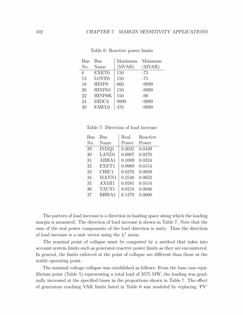
102 CHAPTER 7. MARGIN SENSITIVITY APPLICATIONS
Table 6: Reactive power limits
Bus Bus Maximum MinimumNo. Name (MVAR) (MVAR)
6 EXET0 150 -7513 LOVE0 150 -7518 HINP0 660 -999920 HINP0J 150 -999922 HINP0K 150 -9024 DIDC4 9999 -999939 FAWL0 470 -9999
Table 7: Direction of load increase
Bus Bus Real ReactiveNo. Name Power Power
29 INDQ1 0.2032 0.043930 LAND1 0.0907 0.027031 ABHA1 0.1089 0.032432 EXET1 0.0980 0.015433 CHIC1 0.0276 0.003934 MANN1 0.2540 0.063235 AXMI1 0.0581 0.015436 TAUN1 0.0218 0.004637 BRWA1 0.1379 0.0000
The pattern of load increase is a direction in loading space along which the loading
margin is measured. The direction of load increase is shown in Table 7. Note that the
sum of the real power components of the load direction is unity. Thus the direction
of load increase is a unit vector using the L1 norm.
The nominal point of collapse must be computed by a method that takes into
account system limits such as generator reactive power limits as they are encountered.
In general, the limits enforced at the point of collapse are different than those at the
stable operating point.
The nominal voltage collapse was established as follows: From the base case equi-
librium point (Table 5) representing a total load of 3575 MW, the loading was grad-
ually increased at the specified buses in the proportions shown in Table 7. The effect
of generators reaching VAR limits listed in Table 6 was modeled by replacing ‘PV’
7.3. LOADING MARGIN SENSITIVITY 103
buses with ‘PQ’ buses at the loading at which VAR limits were reached. Transformer
taps were held fixed at the starting ratios. No other changes to the network param-
eters were implemented. In particular, no shunts were adjusted as the loading was
increased. The base case system encountered a voltage collapse at a total load of
5380 MW, and thus the nominal margin is 1805 MW. Prior to voltage collapse, the
PV buses at EXET0, FAWL0, and LOVE0 encountered VAR limits, and the PV bus
at HINP0 was very close to reaching its VAR limit. Table 8 shows the solution at
the nominal point of collapse. Generators that have reached reactive power limits are
indicated in bold face as is the VAR output at HINP0 which is precariously close to
a VAR limit.
The Jacobian of the equilibrium equations with respect to the state variables
at the nominal point of collapse is singular (fold bifurcation). The left eigenvector
corresponding to the zero eigenvalue of the system Jacobian matrix evaluated at
the nominal point of collapse is shown in Table 9, normalized so that the largest
component is unity. This left eigenvector is the normal vector to the set of real
and reactive power injections that correspond to a fold bifurcation of the equilibrium
equations. The left eigenvector indicates that the bus with the greatest influence on
the loading margin is the Indian Queens 132kV bus.
7.3 Loading margin sensitivity
Introduction
This section describes and illustrates the use of loading margin sensitivities to avoid
voltage collapse. The nominal stable operating point and the nominal point of collapse
are described in the previous section.
The derivation of the sensitivity formulas assumes that the system equations re-
main fixed as parameters are varied. In particular, the limits enforced at the point
of collapse are assumed to stay the same as parameters are varied. (A change in the
system limits corresponds to a change in the system equations and the sensitivity
based estimates using the equations valid at the nominal nose can become inaccurate
when the parameters change sufficiently so that the equations change.)
For this study, when a generator represented by a ‘PV’ bus reaches a reactive power
limit, it is converted to a ‘PQ’ bus, effectively changing the equilibrium equations
modeling the system. In [GDA97] and [GDA98], the major cause for inaccuracies of
the sensitivity based estimates is shown to be generator reactive power limits changing
as parameters are varied.
The case studied here is indeed challenging since the generator at HINP0 is very

104 CHAPTER 7. MARGIN SENSITIVITY APPLICATIONS
Table 8: Nominal point of collapse
Bus Bus Bus Voltage Angle Load GenerationNo. Name Type (p.u.) (degrees) (MW) (MVAR) (MW) (MVAR)
1 INDQ4 PQ 0.832 -29.32 - - - -2 LAND4 PQ 0.826 -29.88 - - - -3 ABHA4T PQ 0.863 -27.28 - - - -4 ABHA4U PQ 0.851 -28.03 - - - -5 EXET4 PQ 0.895 -25.03 - - - -6 EXET0 PQ 0.948 -25.03 - - - 150.07 TAUN4J PQ 0.914 -23.43 - - - -8 TAUN4K PQ 0.915 -23.71 - - - -9 AXMI4 PQ 0.899 -24.20 - - - -10 CHIC4 PQ 0.907 -22.47 - - - -11 MANN4 PQ 0.916 -20.09 - - - -12 LOVE4 PQ 0.958 -14.54 422.0 -63.8 - -13 LOVE0 PQ 1.008 -14.54 - - - 150.014 NURS4 PQ 0.957 -14.44 200.4 48.4 - -15 FLEE4 PQ 0.972 -17.45 469.1 96.5 - -60.016 BRLE4 PQ 0.982 -18.12 - - -108.8 86.317 HINP4 PQ 0.937 -21.56 - - - -18 HINP0 PV 1.000 -14.50 - - 1099.1 650.019 HINP2J PQ 0.924 -21.67 - - - -20 HINP0J PV 1.000 -11.38 - - 207.8 107.721 HINP2K PQ 0.924 -21.65 - - - -22 HINP0K PV 1.000 -11.35 - - 207.8 107.623 MELK4 PQ 0.963 -20.77 - - -392.6 42.524 DIDC4 PV 1.005 -18.30 - - -38.6 582.125 BOLN4 PQ 0.958 -8.433 518.5 117.3 - -26 NINF4 PQ 0.971 -2.317 358.4 153.1 - -27 BRWA2Q PQ 0.912 -22.70 - - - -28 BRWA2R PQ 0.912 -22.66 - - - -29 INDQ1 PQ 0.569 -61.26 661.6 142.9 - -30 LAND1 PQ 0.717 -43.48 295.4 87.8 - -31 ABHA1 PQ 0.786 -39.44 354.4 105.3 - -32 EXET1 PQ 0.787 -37.56 319.0 50.2 - -33 CHIC1 PQ 0.852 -25.36 89.8 12.5 - -34 MANN1 PQ 0.821 -33.42 827.0 205.7 - -35 AXMI1 PQ 0.839 -29.97 189.0 50.2 - -36 TAUN1 PQ 0.845 -33.64 70.9 15.1 - -37 BRWA1 PQ 0.883 -34.07 449.0 - - -38 FAWL4 PQ 0.957 -13.97 156.0 57.4 - -39 FAWL0 PQ 0.983 -6.965 - - 1806.5 470.040 DUNG4 AV 0.996 3.400 - - 2748.7 601.2

7.3. LOADING MARGIN SENSITIVITY 105
Table 9: Left eigenvector corresponding to the zero eigenvalue of the system Jacobianat the nominal point of collapse
Bus Bus Real ReactiveNo. Name Power Power1 INDQ4 0.1172 0.30412 LAND4 0.1227 0.29363 ABHA4T 0.0899 0.22404 ABHA4U 0.0984 0.23865 EXET4 0.0683 0.17106 EXET0 0.0683 0.15307 TAUN4J 0.0552 0.14398 TAUN4K 0.0568 0.14459 AXMI4 0.0625 0.154510 CHIC4 0.0522 0.133711 MANN4 0.0404 0.105612 LOVE4 0.0206 0.054213 LOVE0 0.0206 0.049114 NURS4 0.0207 0.059315 FLEE4 0.0238 0.037316 BRLE4 0.0242 0.030717 HINP4 0.0421 0.103118 HINP0 0.0281 0.000019 HINP2J 0.0450 0.091620 HINP0J 0.0258 0.000021 HINP2K 0.0449 0.091522 HINP0K 0.0257 0.000023 MELK4 0.0341 0.065124 DIDC4 0.0221 0.000025 BOLN4 0.0094 0.033726 NINF4 0.0027 0.015727 BRWA2Q 0.0502 0.096728 BRWA2R 0.0500 0.096629 INDQ1 0.9086 1.000030 LAND1 0.3177 0.482031 ABHA1 0.2107 0.309132 EXET1 0.1730 0.247933 CHIC1 0.0660 0.136434 MANN1 0.0988 0.135735 AXMI1 0.0955 0.167036 TAUN1 0.1122 0.157237 BRWA1 0.1085 0.138538 FAWL4 0.0198 0.061739 FAWL0 0.0048 0.059740 DUNG4 0.0000 0.0000

106 CHAPTER 7. MARGIN SENSITIVITY APPLICATIONS
close to a limit at the nominal point of collapse. It is likely that for changes in some
parameters, the maximum VAR limit at HINP0 will be reached prior to the new
collapse point.
Computation of linear sensitivity
The linear estimate of the change in loading margin (∆L) resulting from a change to
an arbitrary parameter (∆p) is:
∆L = Lp∆p =−wFp∆p
wFλk(132)
where :
• Lp is the sensitivity of the loading margin with respect to the parameter.
• F are the power system equilibrium equations (real and reactive power balance
at each bus) that apply at the nose. In particular, F accounts for the power
system limits enforced at the nose.
• Fλ, the derivative of F with respect to the load parameters. For constant power
load models Fλ is a diagonal matrix with ones in the rows corresponding to
buses with loads.
• Fp, the derivative of the equilibrium equations with respect to the parameter
p at the nominal nose point. The parameter can be a vector and then Fp is a
matrix.
• w, the left eigenvector corresponding to the zero eigenvalue of the system Jaco-
bian Fx (Fx evaluated at a fold bifurcation is singular [IEEE1, DCL, Davos]).
• k, the unit vector in the direction of load increase. k also defines the direction in
which the loading margin is measured. The direction of load increase is shown
in Table 7.
The denominator of (132) is a scaling factor that is the same for all parameter
changes. The linear sensitivity can be improved with a quadratic estimate, derived
and explained in [GDA97].
Sensitivity with respect to load variation
Table 9 shows the left eigenvector corresponding to the zero eigenvalue of the system
Jacobian evaluated at the nominal fold point. This left eigenvector indicates that the

7.3. LOADING MARGIN SENSITIVITY 107
voltage collapse is most affected by the load at the 132 KV Indian Queens bus. There
are several situations in which the sensitivity of the margin to voltage collapse with
respect to the load would be of interest.
There is usually uncertainty in the metering or forecast of loads. By computing
the sensitivity to the load, one can estimate the effects of inaccuracy in the nominal
values used. Secondly, it might be possible to interrupt load at a bus, and it would be
useful to know how much margin can be gained for each MW of load shed. Finally,
the sensitivity computation identifies buses that are good candidates for planned
improvements. For example, load margin sensitivity can specify good locations for
VAR support or areas where interruptible contracts can be most profitable.
Methods
The loading margin corresponding to various loads of the same power factor at the
132KV Indian Queens Bus is computed by the same continuation method used to
obtain the nominal fold bifurcation. The results are compared to those obtained
using the linear sensitivity formulas evaluated at the nominal fold bifurcation.
There is 294 MW of 0.98 power factor load at the Indian Queens 132KV bus at
the nominal stable operating point. Results are obtained for variation of ±50MW, or
(±17%) of the base load.
Results
The solid lines in Figures 16 and 17 are the linear estimates for the loading margin
variation as a function of the load shed. The dots in Figures 16 and 17 represent the
actual values of the loading margin as computed by the continuation method.
Figure 16 shows the effects on the loading margin for increasing the load at INDQ0
by 10 MW increments at power factor 0.98. The dots represent the collapse points
as computed by continuation, and the line represents the linear estimate. Figure 17
shows the effects on the loading margin for decreasing the load at INDQ0 by 10 MW
increments at power factor of 0.98.
The agreement between the linear estimates and the actual margins is excellent
over the entire range, but better for the increase in load than the reduction of load.
Closer inspection showed that a reduction of any more than 3 MW caused the gener-
ator at HINP0 to reach its reactive power limit prior to voltage collapse. The nearby
VAR limit at HINPO affected the accuracy of the estimates as speculated. Although
the effect is recognizable as a deviation from the linear estimate, the magnitude of the
error is insignificant. (In fact, the HINP0 VAR limit causes an immediate instability
(see section 7.5). The immediate instability occurs closer to the estimate point of
108 CHAPTER 7. MARGIN SENSITIVITY APPLICATIONS
collapse than the fold point computed and is shown by the circles in Figure 18.)
Sensitivity with respect to VAR limits
Computation of the nominal voltage collapse point showed that Buses EXET0, FAWL0,
and LOVE0 all encounter VAR limits. We find out from sensitivities how the loading
margin to voltage collapse would change if these limits were different.
Methods
The magnitude of the components of the zero left eigenvector (Table 9) corresponding
to reactive power injection indicates that of the three generators that encounter VAR
limits between the nominal stable operating point and the point of collapse, the
generator at the 132 KV bus at Exeter has the greatest influence on the margin
to collapse. The loading margin corresponding to various maximum reactive power
limits at the 132KV Exeter Bus is computed by the same continuation method used
to obtain the nominal fold bifurcation. The results are compared to those obtained
using the linear sensitivity formula evaluated at the nominal fold bifurcation.
The nominal maximum reactive power limit at the Exeter 132KV bus is 150
MVARs. Results are obtained for a variation of 30 MVARs, or (±20%) of the nominal
limit.
Results
The solid lines in Figure 19 shows the linear estimate for the loading margin variation
as a function of the maximum reactive power limit at the 132 KV Exeter bus. The
dots in Figure 19 represent the actual values of the loading margin as computed by
the continuation method. The agreement between the linear estimates and the actual
margins is excellent over the entire range.
7.4 Contingency ranking for voltage collapse
The sensitivity formulas (132) of the previous section can be used to estimate the
effects of contingencies on the margin to voltage collapse. In this case the parameter
p is a vector representing the line admittance, and instead of looking at the effect of
small deviations, the change in the parameter is 100%.

7.4. CONTINGENCY RANKING FOR VOLTAGE COLLAPSE 109
1650
1700
1750
1800
0 10 20 30 40 50
Actual
Linear
Loa
ding
mar
gin
(MW
)
Load Increase(MW)
Figure 16: Effect of load increase at Indian Queens on the loading margin to voltagecollapse

110 CHAPTER 7. MARGIN SENSITIVITY APPLICATIONS
1800
1850
1900
1950
0 10 20 30 40 50
Actual
Linear
Loa
ding
mar
gin
(MW
)
Load Decrease(MW)
Figure 17: Effect of load decrease at Indian Queens on the loading margin to voltagecollapse
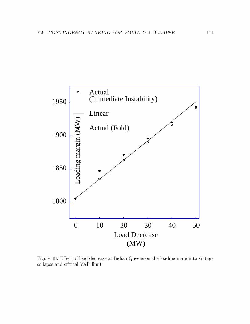
7.4. CONTINGENCY RANKING FOR VOLTAGE COLLAPSE 111
1800
1850
1900
1950
0 10 20 30 40 50
Actual(Immediate Instability)
Linear
Actual (Fold)
Loa
ding
mar
gin
(MW
)
Load Decrease(MW)
Figure 18: Effect of load decrease at Indian Queens on the loading margin to voltagecollapse and critical VAR limit

112 CHAPTER 7. MARGIN SENSITIVITY APPLICATIONS
1780
1790
1800
1810
1820
-40 -30 -20 -10 0 10 20 30
Actual
Linear
Loa
ding
mar
gin
(MW
)
VAR Limit Change(MVAR)
Figure 19: Effect of variation in VAR limits at Exeter on the loading margin to voltagecollapse
7.4. CONTINGENCY RANKING FOR VOLTAGE COLLAPSE 113
Method
The estimates for the effects of contingencies were computed as described in [GDA98].
The actual margins resulting from the contingencies were computed by first identify-
ing a stable post contingency equilibrium at the base case loading and then gradually
increasing the load and accounting for VAR limits until a voltage collapse due to fold
bifurcation of the equilibrium equations was found.
Radial line outages are a special case in which the derived formulas do not strictly
apply since the post outage network will not be connected. We suggest that the
contingency list be first screened to identify radial lines, and that these outages be
analyzed and ranked separately from the other contingencies. 1
Results
Table 10 compares the estimates to the actual margins for all non-radial line outages
resulting in at least a 75 MW reduction in loading margin. The ranks correspond to
the rank of each outage among all other non-radial line outages. Table 11 compares
the estimates to the actual margins for all radial line outages, with ranking shown
among only radial lines. The two most critical radial line outages are among the
most critical line outages and are identified as so. However, the estimates for the
radial line outages tend to be better than the estimates for non-radial outages, and
so the moderate radial outages tend to be ranked too high when included with all
line outages. Table 12 shows the remaining line outages. Outages mis-grouped by
the estimates are shown in bold face. The radial outages were all ranked correctly.
For the four outages causing less than a 10 MW change in margin, the mean
error for the linear estimate was 3.0 MW and the maximum error was 4 MW. For
the ten outages causing between a 10 MW and 20 MW change in margin, the mean
error was 3.9 MW and the maximum error was 13 MW. For the thirteen outages
causing between a 20 MW and 45 MW change in margin, the mean error was 10.4
MW and the maximum error was 26 MW. The estimates captured the thirteen worst
non-radial line outages, all causing greater than 60 MW change in the margin. The
worst results pertained to the outages between BRWA2Q and HINP2J (27.19.1) and
BRWA2R and HINP2K (28.21.1).
As noted in [GDA98], the major cause for inaccuracy was due to changes in the
1For the system used for this report, all radial line outages result in isolation of a single bus. Theestimates were then obtained by assuming a reduced system in which the flows on the outaged lineappear as loads at the bus still connected to the network following the outage, and the left eigenvectorcomponents for that bus adjusted to include the components corresponding to the isolated bus. Theoutage estimates then correspond to the case of adding load at a bus.

114 CHAPTER 7. MARGIN SENSITIVITY APPLICATIONS
Table 10: Estimated and actual changes in the loading margin to fold bifurcationresulting from severe non-radial line outages
(nominal loading margin = 1805 MW)
Actual Estimate VARLine Margin Change Linear Quadratic LimitedOutage MW MW (rank) Generators29.30.1 1464 -341 (1) -172 (1) -266 (1) EXET0
4.5.1 1555 -250 (2) -82 (4) -133 (4) EXET0,FAWL0
7.17.1 1635 -170 (3) -52 (9) -87 (7) EXET0,FAWL0,LOVE0
8.17.1 1637 -168 (4) -54 (8) -89 (6) EXET0,FAWL0,LOVE0
1.7.1 1643 -162 (5) -129 (2) -154 (2) EXET0,FAWL0
1.8.1 1643 -162 (6) -129 (3) -154 (3) EXET0,FAWL0
11.38.1 1650 -155 (7) -70 (5) -101 (5) EXET0,FAWL0,HINP0
2.4.1 1653 -152 (8) -48 (11) -75 (10) EXET0,FAWL0
3.5.1 1653 -152 (9) -51 (10) -80 (9) EXET0,FAWL0
11.12.1 1700 -105 (10) -61 (6) -83 (8) EXET0,FAWL0,HINP0
1.3.1 1718 -87 (11) -56 (7) -71 (11) EXET0,FAWL0
set of limits that apply at the point of collapse. This system proved to be a most
challenging case, since all but nine outages forced a change in the limits applied at
the nose.
As expected, often the change in VAR limits involved the HINP0 bus precariously
close to a limit at the nominal point of collapse. In many instances, encountering this
limit caused an immediate instability and this is addressed in section 7.5.
7.5 Voltage collapse due to VAR limits
The previous sections and the theory presented in [GDA97, GDA98] associate voltage
collapse of the electric power system with a fold bifurcation of the equilibrium equa-
tions used to model the system. Experience [DCL, Davos, FOC90, FFOCH, HSS,
HawPhD] has shown that the VAR limitations of generators are associated with volt-
age instability, and computational experience shows that the effect of changing PV
buses in the equilibrium model of the power system to PQ buses often reduces the
loading margin to voltage collapse.
In some cases, when the system loading is high, the effect of changing a PV bus
to a PQ bus causes the margin to the fold bifurcation to increase. Upon application
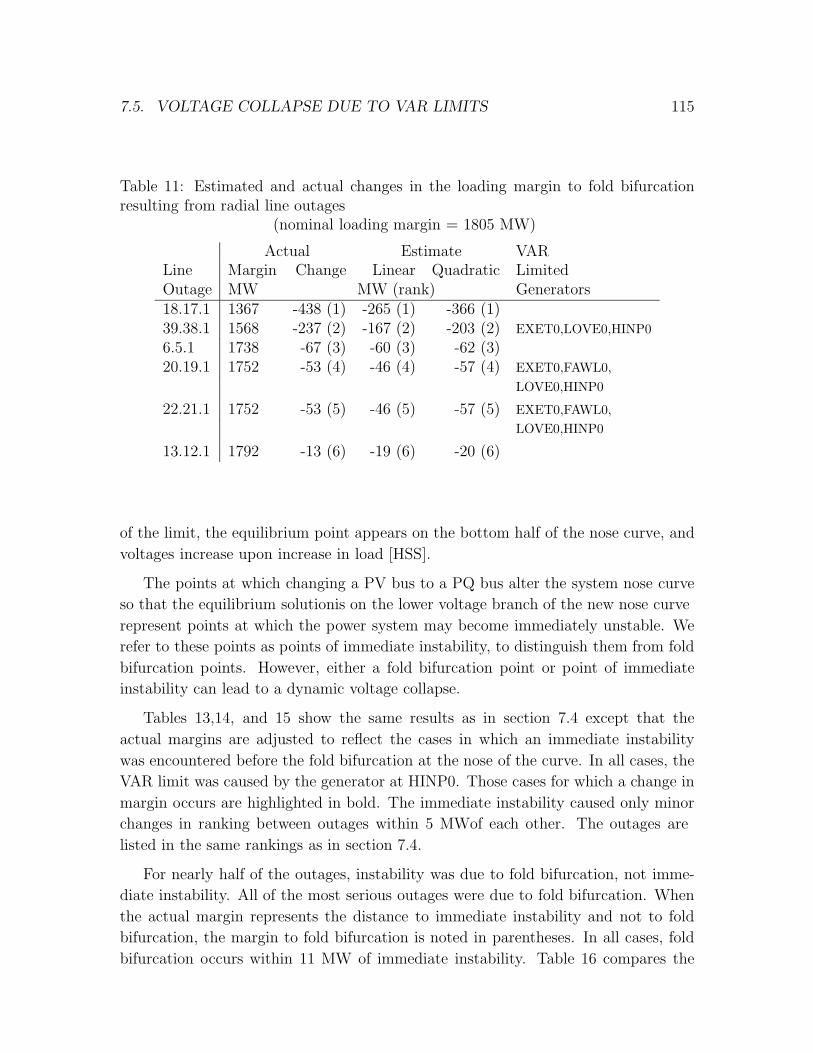
7.5. VOLTAGE COLLAPSE DUE TO VAR LIMITS 115
Table 11: Estimated and actual changes in the loading margin to fold bifurcationresulting from radial line outages
(nominal loading margin = 1805 MW)
Actual Estimate VARLine Margin Change Linear Quadratic LimitedOutage MW MW (rank) Generators18.17.1 1367 -438 (1) -265 (1) -366 (1)39.38.1 1568 -237 (2) -167 (2) -203 (2) EXET0,LOVE0,HINP0
6.5.1 1738 -67 (3) -60 (3) -62 (3)20.19.1 1752 -53 (4) -46 (4) -57 (4) EXET0,FAWL0,
LOVE0,HINP0
22.21.1 1752 -53 (5) -46 (5) -57 (5) EXET0,FAWL0,
LOVE0,HINP0
13.12.1 1792 -13 (6) -19 (6) -20 (6)
of the limit, the equilibrium point appears on the bottom half of the nose curve, and
voltages increase upon increase in load [HSS].
The points at which changing a PV bus to a PQ bus alter the system nose curve
so that the equilibrium solution is on the lower voltage branch of the new nose curve
represent points at which the power system may become immediately unstable. We
refer to these points as points of immediate instability, to distinguish them from fold
bifurcation points. However, either a fold bifurcation point or point of immediate
instability can lead to a dynamic voltage collapse.
Tables 13,14, and 15 show the same results as in section 7.4 except that the
actual margins are adjusted to reflect the cases in which an immediate instability
was encountered before the fold bifurcation at the nose of the curve. In all cases, the
VAR limit was caused by the generator at HINP0. Those cases for which a change in
margin occurs are highlighted in bold. The immediate instability caused only minor
changes in ranking between outages within 5 MW of each other. The outages are
listed in the same rankings as in section 7.4.
For nearly half of the outages, instability was due to fold bifurcation, not imme-
diate instability. All of the most serious outages were due to fold bifurcation. When
the actual margin represents the distance to immediate instability and not to fold
bifurcation, the margin to fold bifurcation is noted in parentheses. In all cases, fold
bifurcation occurs within 11 MW of immediate instability. Table 16 compares the

116 CHAPTER 7. MARGIN SENSITIVITY APPLICATIONS
Table 12: Estimated and actual changes in the loading margin to fold bifurcationresulting from less severe non-radial line outages
(nominal loading margin = 1805 MW)
Actual Estimate VARLine Margin Change Linear Quadratic LimitedOutage MW Generators
31.30.1 1735 -70 -33 -51 EXET0,FAWL09.11.1 1739 -66 -39 -51 EXET0,FAWL0,HINP027.19.1 1747 -58 -6 -8 EXET0,FAWL0,LOVE0,HINP028.21.1 1748 -57 -5 -8 EXET0,FAWL0,LOVE0,HINP05.7.1 1752 -53 -27 -37 EXET0,FAWL0,LOVE05.8.1 1755 -50 -26 -36 EXET0,FAWL0,LOVE010.11.1 1757 -48 -21 -29 EXET0,FAWL0,HINP05.10.1 1759 -46 -29 -37 EXET0,FAWL0,HINP016.24.1 1764 -41 -28 -39 EXET0,FAWL0,LOVE0,HINP016.24.2 1764 -41 -28 -39 EXET0,FAWL0,LOVE0,HINP012.38.1 1767 -38 -12 -12 EXET0,FAWL0,LOVE0,HINP012.38.2 1767 -3 -12 -12 EXET0,FAWL0,LOVE0,HINP017.23.1 1771 -34 -24 -29 EXET0,FAWL0,HINP017.23.2 1771 -34 -24 -29 EXET0,FAWL0,HINP026.40.2 1775 -30 -17 -27 EXET0,FAWL0,LOVE0,HINP026.40.1 1775 -30 -17 -27 EXET0,FAWL0,LOVE0,HINP037.36.1 1777 -28 -4 -8 EXET0,FAWL0,LOVE025.26.1 1778 -27 -17 -25 EXET0,FAWL0,LOVE0,HINP025.26.2 1778 -27 -17 -25 EXET0,FAWL0,LOVE0,HINP05.9.1 1778 -27 -12 -14 EXET0,FAWL0,HINP032.36.1 1779 -26 -14 -21 EXET0,FAWL0,LOVE016.23.1 1785 -20 -18 -23 EXET0,FAWL0,LOVE0,HINP016.23.2 1785 -20 -18 -23 EXET0,FAWL0,LOVE0,HINP012.25.1 1787 -18 -16 -22 EXET0,FAWL0,LOVE0,HINP012.25.2 1787 -18 -16 -22 EXET0,FAWL0,LOVE0,HINP031.32.1 1787 -18 -5 -8 EXET0,FAWL0,LOVE01.2.1 1791 -14 -14 -13 EXET0,FAWL0,LOVE0,HINP015.16.1 1791 -14 -7 -9 EXET0,FAWL0,LOVE0,HINP015.16.2 1791 -14 -7 -9 EXET0,FAWL0,LOVE0,HINP012.15.1 1793 -12 -14 -20 EXET0,FAWL0,LOVE0,HINP012.15.2 1793 -12 -14 -20 EXET0,FAWL0,LOVE0,HINP012.14.1 1800 -5 -4 -4 EXET0,FAWL0,LOVE0,HINP014.38.1 1800 -5 -2 -2 EXET0,FAWL0,LOVE0,HINP017.19.1 1809 4 0 2 EXET0,FAWL0,LOVE017.21.1 1809 4 0 2 EXET0,FAWL0,LOVE0

7.6. RANKING FOR VOLTAGE COLLAPSE DUE TO VAR LIMITS 117
Table 13: Estimated and actual changes in the loading margin to voltage collapseresulting from severe non-radial line outages
(nominal loading margin = 1805 MW)
Actual Estimate VARLine Margin Change Linear Quadratic LimitedOutage MW MW (rank) Generators29.30.1 1464 -341 (1) -172 (1) -266 (1) EXET0
4.5.1 1555 -250 (2) -82 (4) -133 (4) EXET0,FAWL0
7.17.1 1635 -170 (3) -52 (9) -87 (7) EXET0,FAWL0,LOVE0
8.17.1 1637 -168 (4) -54 (8) -89 (6) EXET0,FAWL0,LOVE0
1.7.1 1643 -162 (5) -129 (2) -154 (2) EXET0,FAWL0
1.8.1 1643 -162 (6) -129 (3) -154 (3) EXET0,FAWL0
11.38.1 1650 -155 (7) -70 (5) -101 (5) EXET0,FAWL0,HINP0
2.4.1 1653 -152 (8) -48 (11) -75 (10) EXET0,FAWL0
3.5.1 1653 -152 (9) -51 (10) -80 (9) EXET0,FAWL0
11.12.1 1699 (1700) -106 (10) -61 (6) -83 (8) EXET0,FAWL0,HINP0
1.3.1 1718 -87 (11) -56 (7) -71 (11) EXET0,FAWL0
loading margins to fold bifurcation with the loading margins to immediate instabil-
ity for each outage at which an immediate instability was observed prior to voltage
collapse due to fold bifurcation.
Since all cases of immediate instability resulted from the generator at HINP0
hitting a VAR limit (although this did not always result in an immediate instability)
it is natural to ask how the contingencies affect the loading margin to the HINP0
VAR limit, as opposed to the loading margin to the fold bifurcation. This topic is
addressed in section 7.6.
7.6 Contingency ranking for voltage collapse due
to VAR limits
The sensitivity computations can be easily extended to the case were the voltage
collapse is an immediate instability due to a VAR limit rather than a fold bifurcation.
The derivations of the sensitivity formulas in [GDA97] required the description of
a manifold in which each point on the manifold corresponded to a point of fold
bifurcation. The normal vector to this surface is defined by the zero left eigenvector

118 CHAPTER 7. MARGIN SENSITIVITY APPLICATIONS
Table 14: Estimated and actual changes in the loading margin to voltage collapseresulting from radial line outages
(nominal loading margin = 1805 MW)
Actual Estimate VARLine Margin Change Linear Quadratic LimitedOutage MW MW (rank) Generators18.17.1 1367 -438 (1) -265 (1) -366 (1)39.38.1 1568 -237 (2) -167 (2) -203 (2) EXET0,LOVE0,HINP0
6.5.1 1738 -67 (3) -60 (3) -62 (3)
20.19.1 1750 (1752) -55 (4) -46 (4) -57 (4) EXET0,FAWL0,
LOVE0,HINP0
22.21.1 1750 (1752) -55 (5) -46 (5) -57 (5) EXET0,FAWL0,
LOVE0,HINP0
13.12.1 1792 -13 (6) -19 (6) -20 (6)
of the system Jacobian. Similarly we can construct a manifold in which each point
corresponds to the point at which a particular generator is at a VAR limit. The
normal vector to this surface can then be used in the sensitivity formulas to compute
the sensitivity of the margin to encountering a VAR limit.
Computation of nominal point of instability
Computation of the point of immediate instability is similar to computation of a
fold bifurcation point. The same continuation method can be used, and the point of
collapse is the point at which a VAR limit is encountered and upon further increase
in load the system voltages increase. Thus, the immediate instability can be detected
by computing the sensitivity of the bus voltages to the loading factor after application
of the limit. (Note that the software described in [HSS] performs this check to detect
voltage collapse due to fold bifurcation or immediate instability.) It is in general
easier to locate the exact point of encountering a VAR limit than it is to locate the
exact fold bifurcation point. The equations are sparser, a good initial guess for the
eigenvectors is unnecessary, and the Jacobian is less likely to be poorly conditioned
since the power balance equations are not evaluated at a point of singularity.
For this study, the maximum VAR limit at HINP0 was changed from 660 MVAR
to 630 MVAR. The continuation program was run as before, and again, VAR limits
were reached at EXET0, FAWL0, and LOVE0. However, at a loading 5379 MW,
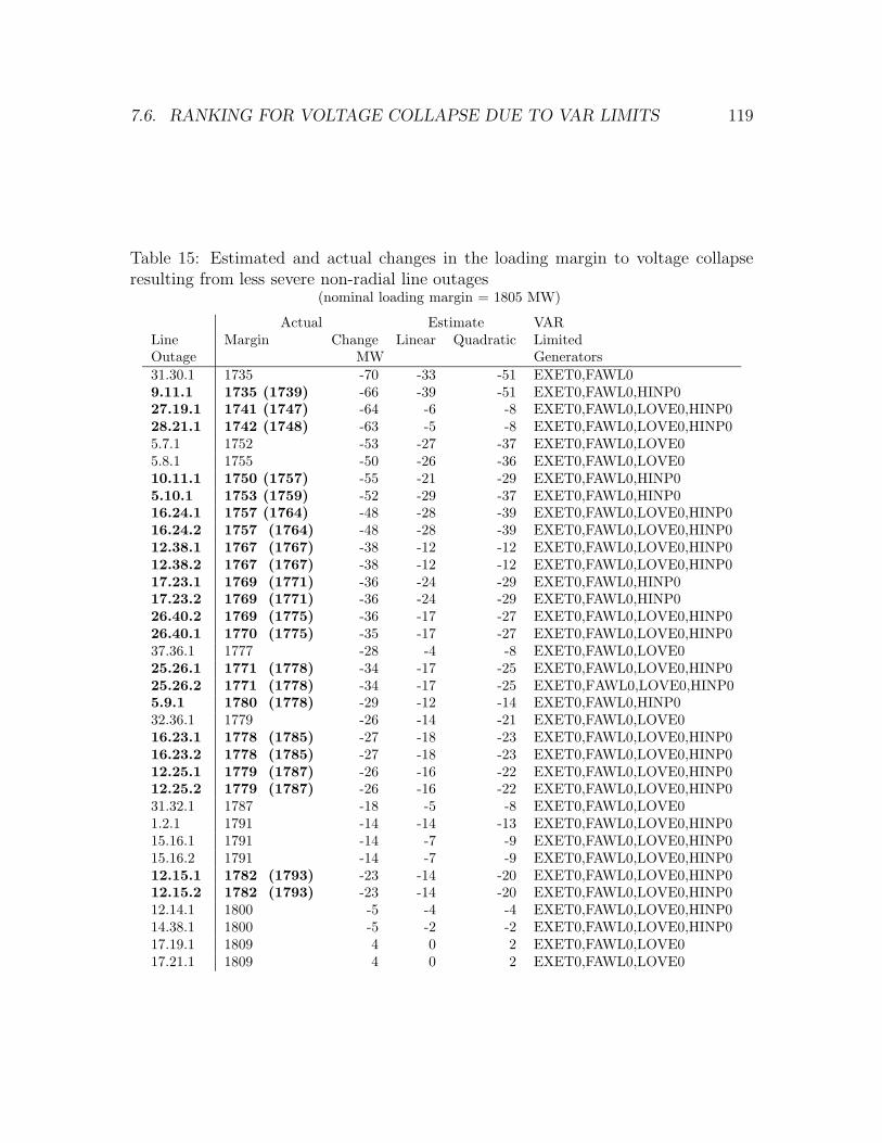
7.6. RANKING FOR VOLTAGE COLLAPSE DUE TO VAR LIMITS 119
Table 15: Estimated and actual changes in the loading margin to voltage collapseresulting from less severe non-radial line outages
(nominal loading margin = 1805 MW)
Actual Estimate VARLine Margin Change Linear Quadratic LimitedOutage MW Generators
31.30.1 1735 -70 -33 -51 EXET0,FAWL09.11.1 1735 (1739) -66 -39 -51 EXET0,FAWL0,HINP027.19.1 1741 (1747) -64 -6 -8 EXET0,FAWL0,LOVE0,HINP028.21.1 1742 (1748) -63 -5 -8 EXET0,FAWL0,LOVE0,HINP05.7.1 1752 -53 -27 -37 EXET0,FAWL0,LOVE05.8.1 1755 -50 -26 -36 EXET0,FAWL0,LOVE010.11.1 1750 (1757) -55 -21 -29 EXET0,FAWL0,HINP05.10.1 1753 (1759) -52 -29 -37 EXET0,FAWL0,HINP016.24.1 1757 (1764) -48 -28 -39 EXET0,FAWL0,LOVE0,HINP016.24.2 1757 (1764) -48 -28 -39 EXET0,FAWL0,LOVE0,HINP012.38.1 1767 (1767) -38 -12 -12 EXET0,FAWL0,LOVE0,HINP012.38.2 1767 (1767) -38 -12 -12 EXET0,FAWL0,LOVE0,HINP017.23.1 1769 (1771) -36 -24 -29 EXET0,FAWL0,HINP017.23.2 1769 (1771) -36 -24 -29 EXET0,FAWL0,HINP026.40.2 1769 (1775) -36 -17 -27 EXET0,FAWL0,LOVE0,HINP026.40.1 1770 (1775) -35 -17 -27 EXET0,FAWL0,LOVE0,HINP037.36.1 1777 -28 -4 -8 EXET0,FAWL0,LOVE025.26.1 1771 (1778) -34 -17 -25 EXET0,FAWL0,LOVE0,HINP025.26.2 1771 (1778) -34 -17 -25 EXET0,FAWL0,LOVE0,HINP05.9.1 1780 (1778) -29 -12 -14 EXET0,FAWL0,HINP032.36.1 1779 -26 -14 -21 EXET0,FAWL0,LOVE016.23.1 1778 (1785) -27 -18 -23 EXET0,FAWL0,LOVE0,HINP016.23.2 1778 (1785) -27 -18 -23 EXET0,FAWL0,LOVE0,HINP012.25.1 1779 (1787) -26 -16 -22 EXET0,FAWL0,LOVE0,HINP012.25.2 1779 (1787) -26 -16 -22 EXET0,FAWL0,LOVE0,HINP031.32.1 1787 -18 -5 -8 EXET0,FAWL0,LOVE01.2.1 1791 -14 -14 -13 EXET0,FAWL0,LOVE0,HINP015.16.1 1791 -14 -7 -9 EXET0,FAWL0,LOVE0,HINP015.16.2 1791 -14 -7 -9 EXET0,FAWL0,LOVE0,HINP012.15.1 1782 (1793) -23 -14 -20 EXET0,FAWL0,LOVE0,HINP012.15.2 1782 (1793) -23 -14 -20 EXET0,FAWL0,LOVE0,HINP012.14.1 1800 -5 -4 -4 EXET0,FAWL0,LOVE0,HINP014.38.1 1800 -5 -2 -2 EXET0,FAWL0,LOVE0,HINP017.19.1 1809 4 0 2 EXET0,FAWL0,LOVE017.21.1 1809 4 0 2 EXET0,FAWL0,LOVE0
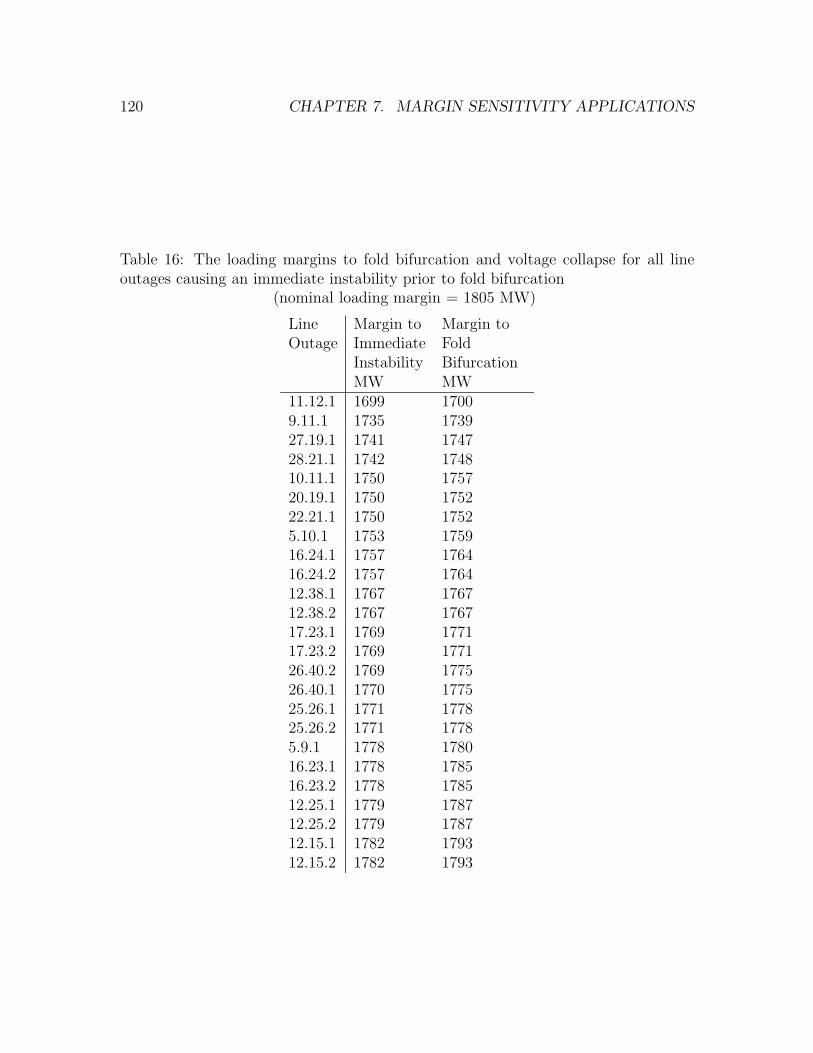
120 CHAPTER 7. MARGIN SENSITIVITY APPLICATIONS
Table 16: The loading margins to fold bifurcation and voltage collapse for all lineoutages causing an immediate instability prior to fold bifurcation
(nominal loading margin = 1805 MW)
Line Margin to Margin toOutage Immediate Fold
Instability BifurcationMW MW
11.12.1 1699 17009.11.1 1735 173927.19.1 1741 174728.21.1 1742 174810.11.1 1750 175720.19.1 1750 175222.21.1 1750 17525.10.1 1753 175916.24.1 1757 176416.24.2 1757 176412.38.1 1767 176712.38.2 1767 176717.23.1 1769 177117.23.2 1769 177126.40.2 1769 177526.40.1 1770 177525.26.1 1771 177825.26.2 1771 17785.9.1 1778 178016.23.1 1778 178516.23.2 1778 178512.25.1 1779 178712.25.2 1779 178712.15.1 1782 179312.15.2 1782 1793
7.6. RANKING FOR VOLTAGE COLLAPSE DUE TO VAR LIMITS 121
HINP0 reaches its VAR limit of 630 MVARS, and the system becomes unstable once
the PV bus is converted to a PQ bus. (A fold bifurcation of the post limit system
occurs at 5385 MW. Note that the point of collapse for the original system occurred
at a loading of 5380 MW due to fold bifurcation.)
Computation of sensitivity
When the voltage collapse is identified with the fold bifurcation of the equilibrium
model, the left zero eigenvector can be used to compute the normal vector to the
surface of bifurcation points in parameter space. Similarly, when the voltage collapse
is identified with the immediate instability due to application of a VAR limit, there
is a normal vector in parameter space to the surface of points at which the critical Q
limit is reached. Chapter 4 details the computation of this vector for general limits.
In short, when equation (132) is evaluated with the vector w computed at the critical
VAR limit point (as opposed to at the fold bifurcation point), ∆L reflects the linear
estimate of the change in margin to the VAR limit for the change in parameter ∆p.
Table 17 compares the VAR limit normal vector N to the zero left eigenvector W.
The angle between N and W is 4.6 degrees. Note that it is considerably easier to
compute N than W. There is no need to compute a Hessian term and computation
of N does not require a good initial guess.
When the sensitivity computations and contingency rankings were repeated using
N in place of W, no significant changes were observed. Tables 18 and 19 compare the
linear estimates for the change in margin resulting from the lines outages computed
with both the left zero eigenvector, W, at the original fold bifurcation point, and
the normal vector to the VAR limit set, N, with the actual margins to instability
for the original system. Note that there is very little difference in the estimates, and
the top twelve contingencies are ranked the same except for two contingencies with a
difference of less than 1 MW are switched. In each case limited by fold bifurcation,
the estimate computed with the zero left eigenvector is better than the estimate
computed with the normal vector. For the one contingency of the top twelve limited
by immediate instability, the VAR limit normal vector is superior.
Table 19 shows the less critical contingencies which tend to be limited by im-
mediate instability as opposed to fold bifurcation. The estimates are very similar,
seldom differing by more than 5 MW. However, the estimates computed with the
normal vector to the VAR limit set are better than those computed with the zero left
eigenvector for the cases that were limited by immediate instability.
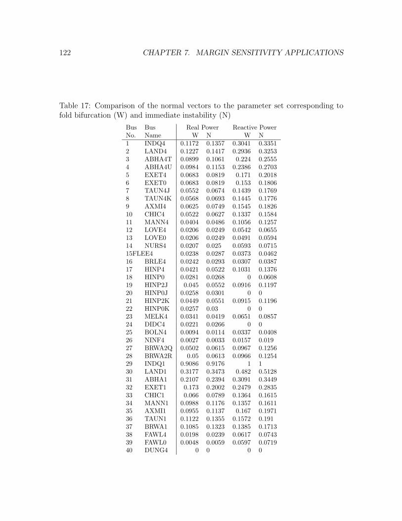
122 CHAPTER 7. MARGIN SENSITIVITY APPLICATIONS
Table 17: Comparison of the normal vectors to the parameter set corresponding tofold bifurcation (W) and immediate instability (N)
Bus Bus Real Power Reactive PowerNo. Name W N W N1 INDQ4 0.1172 0.1357 0.3041 0.33512 LAND4 0.1227 0.1417 0.2936 0.32533 ABHA4T 0.0899 0.1061 0.224 0.25554 ABHA4U 0.0984 0.1153 0.2386 0.27035 EXET4 0.0683 0.0819 0.171 0.20186 EXET0 0.0683 0.0819 0.153 0.18067 TAUN4J 0.0552 0.0674 0.1439 0.17698 TAUN4K 0.0568 0.0693 0.1445 0.17769 AXMI4 0.0625 0.0749 0.1545 0.182610 CHIC4 0.0522 0.0627 0.1337 0.158411 MANN4 0.0404 0.0486 0.1056 0.125712 LOVE4 0.0206 0.0249 0.0542 0.065513 LOVE0 0.0206 0.0249 0.0491 0.059414 NURS4 0.0207 0.025 0.0593 0.071515 FLEE4 0.0238 0.0287 0.0373 0.046216 BRLE4 0.0242 0.0293 0.0307 0.038717 HINP4 0.0421 0.0522 0.1031 0.137618 HINP0 0.0281 0.0268 0 0.060819 HINP2J 0.045 0.0552 0.0916 0.119720 HINP0J 0.0258 0.0301 0 021 HINP2K 0.0449 0.0551 0.0915 0.119622 HINP0K 0.0257 0.03 0 023 MELK4 0.0341 0.0419 0.0651 0.085724 DIDC4 0.0221 0.0266 0 025 BOLN4 0.0094 0.0114 0.0337 0.040826 NINF4 0.0027 0.0033 0.0157 0.01927 BRWA2Q 0.0502 0.0615 0.0967 0.125628 BRWA2R 0.05 0.0613 0.0966 0.125429 INDQ1 0.9086 0.9176 1 130 LAND1 0.3177 0.3473 0.482 0.512831 ABHA1 0.2107 0.2394 0.3091 0.344932 EXET1 0.173 0.2002 0.2479 0.283533 CHIC1 0.066 0.0789 0.1364 0.161534 MANN1 0.0988 0.1176 0.1357 0.161135 AXMI1 0.0955 0.1137 0.167 0.197136 TAUN1 0.1122 0.1355 0.1572 0.19137 BRWA1 0.1085 0.1323 0.1385 0.171338 FAWL4 0.0198 0.0239 0.0617 0.074339 FAWL0 0.0048 0.0059 0.0597 0.071940 DUNG4 0 0 0 0
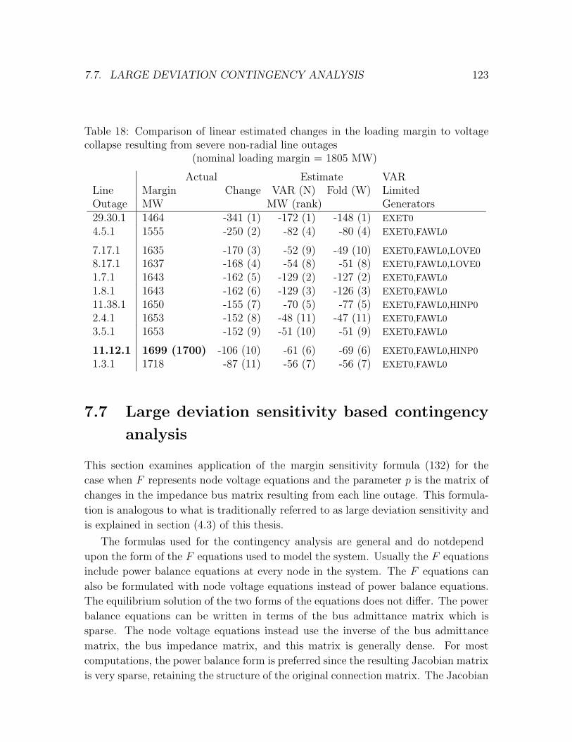
7.7. LARGE DEVIATION CONTINGENCY ANALYSIS 123
Table 18: Comparison of linear estimated changes in the loading margin to voltagecollapse resulting from severe non-radial line outages
(nominal loading margin = 1805 MW)
Actual Estimate VARLine Margin Change VAR (N) Fold (W) LimitedOutage MW MW (rank) Generators29.30.1 1464 -341 (1) -172 (1) -148 (1) EXET0
4.5.1 1555 -250 (2) -82 (4) -80 (4) EXET0,FAWL0
7.17.1 1635 -170 (3) -52 (9) -49 (10) EXET0,FAWL0,LOVE0
8.17.1 1637 -168 (4) -54 (8) -51 (8) EXET0,FAWL0,LOVE0
1.7.1 1643 -162 (5) -129 (2) -127 (2) EXET0,FAWL0
1.8.1 1643 -162 (6) -129 (3) -126 (3) EXET0,FAWL0
11.38.1 1650 -155 (7) -70 (5) -77 (5) EXET0,FAWL0,HINP0
2.4.1 1653 -152 (8) -48 (11) -47 (11) EXET0,FAWL0
3.5.1 1653 -152 (9) -51 (10) -51 (9) EXET0,FAWL0
11.12.1 1699 (1700) -106 (10) -61 (6) -69 (6) EXET0,FAWL0,HINP0
1.3.1 1718 -87 (11) -56 (7) -56 (7) EXET0,FAWL0
7.7 Large deviation sensitivity based contingency
analysis
This section examines application of the margin sensitivity formula (132) for the
case when F represents node voltage equations and the parameter p is the matrix of
changes in the impedance bus matrix resulting from each line outage. This formula-
tion is analogous to what is traditionally referred to as large deviation sensitivity and
is explained in section (4.3) of this thesis.
The formulas used for the contingency analysis are general and do not depend
upon the form of the F equations used to model the system. Usually the F equations
include power balance equations at every node in the system. The F equations can
also be formulated with node voltage equations instead of power balance equations.
The equilibrium solution of the two forms of the equations does not differ. The power
balance equations can be written in terms of the bus admittance matrix which is
sparse. The node voltage equations instead use the inverse of the bus admittance
matrix, the bus impedance matrix, and this matrix is generally dense. For most
computations, the power balance form is preferred since the resulting Jacobian matrix
is very sparse, retaining the structure of the original connection matrix. The Jacobian
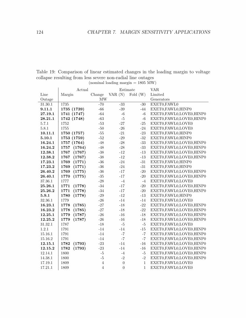
124 CHAPTER 7. MARGIN SENSITIVITY APPLICATIONS
Table 19: Comparison of linear estimated changes in the loading margin to voltagecollapse resulting from less severe non-radial line outages
(nominal loading margin = 1805 MW)
Actual Estimate VARLine Margin Change VAR (N) Fold (W) LimitedOutage MW Generators
31.30.1 1735 -70 -33 -30 EXET0,FAWL09.11.1 1735 (1739) -66 -39 -44 EXET0,FAWL0,HINP027.19.1 1741 (1747) -64 -6 -6 EXET0,FAWL0,LOVE0,HINP028.21.1 1742 (1748) -63 -5 -6 EXET0,FAWL0,LOVE0,HINP05.7.1 1752 -53 -27 -25 EXET0,FAWL0,LOVE05.8.1 1755 -50 -26 -24 EXET0,FAWL0,LOVE010.11.1 1750 (1757) -55 -21 -23 EXET0,FAWL0,HINP05.10.1 1753 (1759) -52 -29 -32 EXET0,FAWL0,HINP016.24.1 1757 (1764) -48 -28 -33 EXET0,FAWL0,LOVE0,HINP016.24.2 1757 (1764) -48 -28 -33 EXET0,FAWL0,LOVE0,HINP012.38.1 1767 (1767) -38 -12 -13 EXET0,FAWL0,LOVE0,HINP012.38.2 1767 (1767) -38 -12 -13 EXET0,FAWL0,LOVE0,HINP017.23.1 1769 (1771) -36 -24 -31 EXET0,FAWL0,HINP017.23.2 1769 (1771) -36 -24 -31 EXET0,FAWL0,HINP026.40.2 1769 (1775) -36 -17 -20 EXET0,FAWL0,LOVE0,HINP026.40.1 1770 (1775) -35 -17 -20 EXET0,FAWL0,LOVE0,HINP037.36.1 1777 -28 -4 -4 EXET0,FAWL0,LOVE025.26.1 1771 (1778) -34 -17 -20 EXET0,FAWL0,LOVE0,HINP025.26.2 1771 (1778) -34 -17 -20 EXET0,FAWL0,LOVE0,HINP05.9.1 1780 (1778) -29 -12 -13 EXET0,FAWL0,HINP032.36.1 1779 -26 -14 -14 EXET0,FAWL0,LOVE016.23.1 1778 (1785) -27 -18 -22 EXET0,FAWL0,LOVE0,HINP016.23.2 1778 (1785) -27 -18 -22 EXET0,FAWL0,LOVE0,HINP012.25.1 1779 (1787) -26 -16 -18 EXET0,FAWL0,LOVE0,HINP012.25.2 1779 (1787) -26 -16 -18 EXET0,FAWL0,LOVE0,HINP031.32.1 1787 -18 -5 -5 EXET0,FAWL0,LOVE01.2.1 1791 -14 -14 -15 EXET0,FAWL0,LOVE0,HINP015.16.1 1791 -14 -7 -7 EXET0,FAWL0,LOVE0,HINP015.16.2 1791 -14 -7 -7 EXET0,FAWL0,LOVE0,HINP012.15.1 1782 (1793) -23 -14 -16 EXET0,FAWL0,LOVE0,HINP012.15.2 1782 (1793) -23 -14 -16 EXET0,FAWL0,LOVE0,HINP012.14.1 1800 -5 -4 -5 EXET0,FAWL0,LOVE0,HINP014.38.1 1800 -5 -2 -2 EXET0,FAWL0,LOVE0,HINP017.19.1 1809 4 0 1 EXET0,FAWL0,LOVE017.21.1 1809 4 0 1 EXET0,FAWL0,LOVE0
7.8. CONCLUSIONS 125
matrix resulting from the node voltage equations is dense.
Note that evaluating the sensitivity formulas assuming the node voltage model
does not require that the equilibrium points or bifurcation points be computed using
those equations. Since the zero set of either the node voltage or power balance equa-
tions is the same, the sparser power balance equations should be used for computing
the nominal boundary point and the normal vectors. The formulas are evaluated as
before, except that a linear transformation is applied to w. The quantity Fp repre-
sents the change in the node voltage equations resulting from a change in the line
impedance p, and is computed using a rank one update of the bus impedance matrix.
The results of the large deviation analysis are compared with those of the pre-
vious analysis for all non-radial line outages. The large deviation sensitivity based
estimates do in general provide bigger estimates and often over estimates for the
changes in margin. However, though of greater magnitude they are no more accurate
than the quadratic estimate, and they appear no better at ranking than the linear
estimate. The large deviation estimates appear more erratic; although the large de-
viation estimate captures 10 of the top 11 contingencies, it mis-ranks a negligible
outage (31.32.1) in the top 11.
The large deviation method utilizes sparse matrix techniques [AST83, SAA85] to
compute the update of the impedance bus matrix and is faster than the quadratic
estimate but not as fast as the linear estimate.
7.8 Conclusions
The methods presented in Chapters 5 and 6 were tested on a small but challenging
case. The nominal voltage collapse occurred at an equilibrium at which a critical VAR
output was precariously close to a limit. It was expected that line outages as well as
small changes in parameters would cause the system to encounter the limit prior to
voltage collapse. This phenomena had previously been associated with inaccuracies
in the estimates and rankings.
For this case, it was shown that the VAR limited changes produced a noticeable
but negligible effect on the estimates. In addition, the formulas were shown to perform
well estimating the effect on the loading margin of altering a generator maximum VAR
limit, illustrating a new application for the methods.
This chapter also tested a new implementation of the sensitivity formulas derived
in Chapter 4 using the node voltage form of the equilibrium equations. Contin-
gency analysis was performed by evaluating the sensitivity formulas for changes in
the impedance matrix resulting from line outages. The initial tests indicate that the
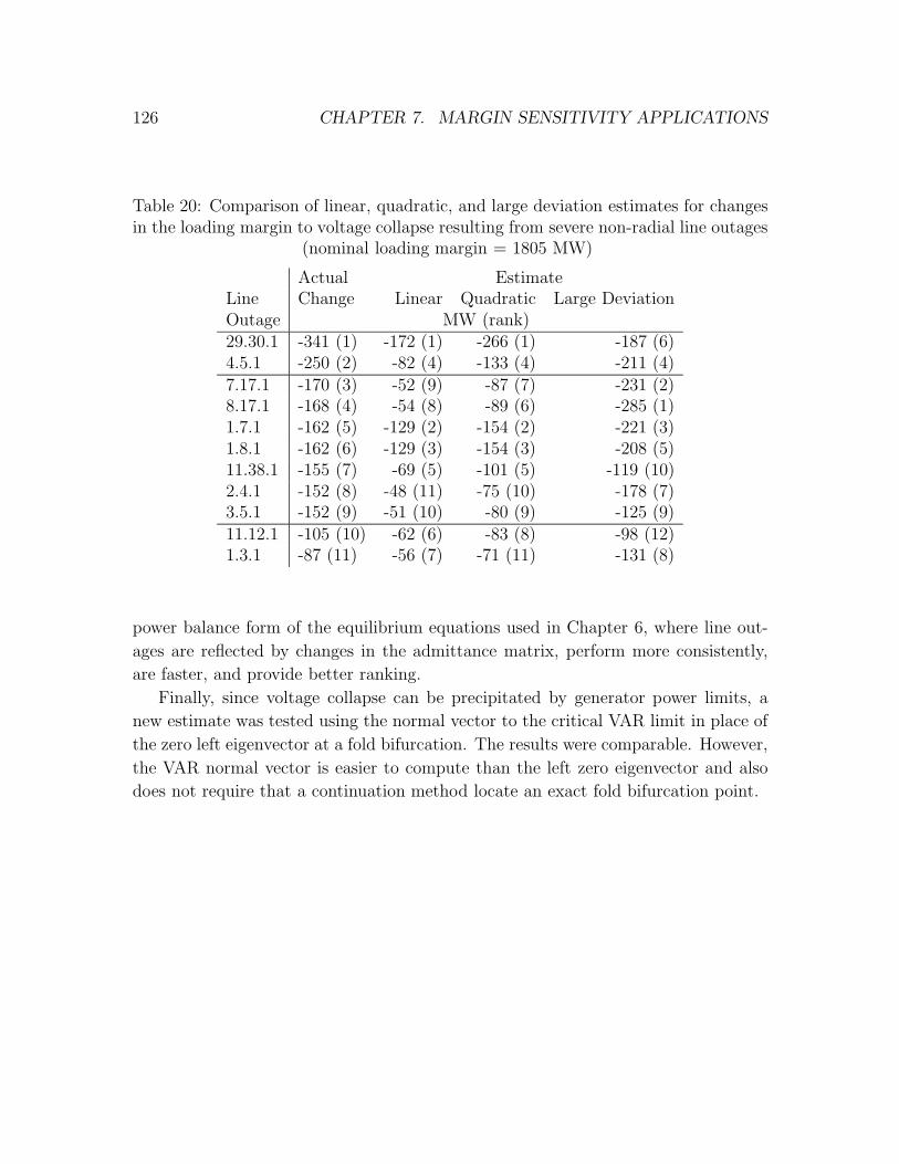
126 CHAPTER 7. MARGIN SENSITIVITY APPLICATIONS
Table 20: Comparison of linear, quadratic, and large deviation estimates for changesin the loading margin to voltage collapse resulting from severe non-radial line outages
(nominal loading margin = 1805 MW)
Actual EstimateLine Change Linear Quadratic Large DeviationOutage MW (rank)29.30.1 -341 (1) -172 (1) -266 (1) -187 (6)4.5.1 -250 (2) -82 (4) -133 (4) -211 (4)
7.17.1 -170 (3) -52 (9) -87 (7) -231 (2)8.17.1 -168 (4) -54 (8) -89 (6) -285 (1)1.7.1 -162 (5) -129 (2) -154 (2) -221 (3)1.8.1 -162 (6) -129 (3) -154 (3) -208 (5)11.38.1 -155 (7) -69 (5) -101 (5) -119 (10)2.4.1 -152 (8) -48 (11) -75 (10) -178 (7)3.5.1 -152 (9) -51 (10) -80 (9) -125 (9)
11.12.1 -105 (10) -62 (6) -83 (8) -98 (12)1.3.1 -87 (11) -56 (7) -71 (11) -131 (8)
power balance form of the equilibrium equations used in Chapter 6, where line out-
ages are reflected by changes in the admittance matrix, perform more consistently,
are faster, and provide better ranking.
Finally, since voltage collapse can be precipitated by generator power limits, a
new estimate was tested using the normal vector to the critical VAR limit in place of
the zero left eigenvector at a fold bifurcation. The results were comparable. However,
the VAR normal vector is easier to compute than the left zero eigenvector and also
does not require that a continuation method locate an exact fold bifurcation point.
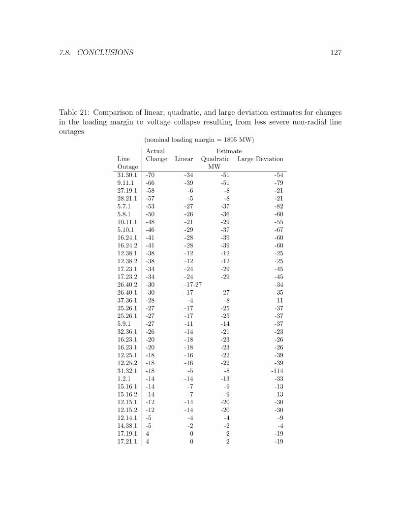
7.8. CONCLUSIONS 127
Table 21: Comparison of linear, quadratic, and large deviation estimates for changesin the loading margin to voltage collapse resulting from less severe non-radial lineoutages
(nominal loading margin = 1805 MW)
Actual EstimateLine Change Linear Quadratic Large DeviationOutage MW
31.30.1 -70 -34 -51 -549.11.1 -66 -39 -51 -7927.19.1 -58 -6 -8 -2128.21.1 -57 -5 -8 -215.7.1 -53 -27 -37 -825.8.1 -50 -26 -36 -6010.11.1 -48 -21 -29 -555.10.1 -46 -29 -37 -6716.24.1 -41 -28 -39 -6016.24.2 -41 -28 -39 -6012.38.1 -38 -12 -12 -2512.38.2 -38 -12 -12 -2517.23.1 -34 -24 -29 -4517.23.2 -34 -24 -29 -4526.40.2 -30 -17 -27 -3426.40.1 -30 -17 -27 -3537.36.1 -28 -4 -8 1125.26.1 -27 -17 -25 -3725.26.1 -27 -17 -25 -375.9.1 -27 -11 -14 -3732.36.1 -26 -14 -21 -2316.23.1 -20 -18 -23 -2616.23.1 -20 -18 -23 -2612.25.1 -18 -16 -22 -3912.25.2 -18 -16 -22 -3931.32.1 -18 -5 -8 -1141.2.1 -14 -14 -13 -3315.16.1 -14 -7 -9 -1315.16.2 -14 -7 -9 -1312.15.1 -12 -14 -20 -3012.15.2 -12 -14 -20 -3012.14.1 -5 -4 -4 -914.38.1 -5 -2 -2 -417.19.1 4 0 2 -1917.21.1 4 0 2 -19

128

129
Chapter 8
Sensitivity of Transfer Capability
Margins
This chapter applies the margin and sensitivity methods to the problem of computing
the transfer capability margin and determining the effect of varying simultaneous
transfers, loading, generation, and reactive power support.
8.1 Introduction
Open access to transmission services requires continual determination of the available
transfer capability (ATC) for each interface of a region or area of the power network.
The ATC indicates how much interarea power transfers can be increased without
compromising system security at a particular moment and for a prescribed interval in
time. The ATC is vital information for the bulk power market. The available transfer
capability is the total transfer capability (TTC) minus existing transfer commitments
together with adjustments to allow some margin of safety. Essentially, transmission
capacity can only be reserved when there is capacity available. While there exists
general agreement concerning the fundamental requirements of the ATC, computa-
tional procedures vary. In addition, once the ATC or TTC is computed under one set
of operating conditions, it is important to determine the effects of varying conditions
and assumptions. It is desirable to understand the effect of increased transfer on
each interface on the ATC of every other interface. This chapter illustrates the use of
sensitivities for estimating the effect on the transfer capability of varying simultane-
ous transfer directions, loading, generation, and reactive power support. The results
apply to the case of transfer limited by line flow limits, voltage limits, generator real
and reactive power limits, and voltage collapse. The computations are illustrated
on a 40 bus, 3 area model and performance is tested with a 1500 bus, twenty area
system. Both systems are derived from a portion of the US grid.
130 CHAPTER 8. SENSITIVITY OF TRANSFER CAPABILITY MARGINS
Previous Work
A concise analysis of ATC computations and current terminology, along with a com-
prehensive bibliography is contained in [Sau97]. Foundational work regarding trans-
mission transfer capability determination is represented in [DGM79, GVHW, LTA72,
LA73, StC53], and, concerning sensitivity and optimal power flow, in [SM79, PPTT,
DT68]. NERC documents [NERC95, NERC96] contain useful terminology and de-
scriptions. The most current information can be found at the OASIS web sites for
each operating region.
Path following methods are used in this chapter to obtain nominal transfer mar-
gins. The details of these methods are explained in Chapter 3 of this thesis. Previous
use of continuation methods for margin determination includes [CA93, CFSB, RHSC,
VC91]. In particular, [RHSC, VC91] illustrate the combined use of continuation meth-
ods and sensitivity analysis for security margin computation. Chapter 1 references
fundamental work in this area.
[GDA97] presents exact analytical margin sensitivity formulas with illustrative
examples including the effect of variation in interarea transfers on the loading margin
to voltage collapse. [WF93] applies sensitivity analysis to the determination of the
contingencies that most limit transfer capability, and motivates the work on contin-
gency analysis presented in [GDA98]. [RAMCJ] demonstrates the use of sensitivity
formulas for locating series compensation to increase power transfer capability.
This chapter continues a research direction in available transfer capability indi-
cated in [Sau97] by applying the margin sensitivity ideas to transfer capability. This
chapter is an extension of the work reported in [GDAS]. This chapter tests the ap-
plication of the methods reported in [GDAS] on a realistic power system example.
8.2 Overview of transfer capability determination
For this chapter we use the main features of the NERC 1995 and 1996 definitions
[NERC95, NERC96]: The power system is judged to be secure for the purpose of
interarea transfer if “all facility loadings are within normal ratings and all voltages are
within normal limits”, the system “remains stable following a disturbance that results
in the loss of any single element”, “the post-contingency system ... has all facility
loadings within emergency ratings and all voltages within emergency limits” [Sau97].
While there exists general agreement concerning the fundamental requirements of
posted transfer capabilities, computational procedures are currently in the process
of refinement. Implementation varies regionally as well as by projected time period
(criteria for next day analysis can differ from seven days ahead). The most current

8.2. OVERVIEW OF TRANSFER CAPABILITY DETERMINATION 131
information can be found at the OASIS web sites for each operating region. This
section outlines the components common to many transfer capability computations
[Sau97].
• Specify Operating Horizon. The time period, or operating horizon, for the
transfer capability computations must be specified. The assumptions used to
establish a base case as well as security criteria can depend upon the operating
horizon.
• Establish Base Case. The base case reflects the most likely condition of the
power system for some point in the (possibly very near) future. Obtaining a
credible base case is not a trivial task since there is always uncertainty with
forecasting the future. The base case must account for the forecast loading
in each area and all scheduled and forced transmission and generator outages
for the identified operating horizon. In addition, transmission reservations and
energy schedules (existing transmission commitments) must be accounted for
in a manner consistent with the operating horizon. Generation dispatch in
each area must be specified along with a stacking order and some criteria to
distribute additional demand arising from deviations to the base case. Normal
and emergency limits for all lines and transformers need to be specified.
• Capacity Benefit Margin Determination Reliability criteria require that a
portion of the total transfer capability be reserved to meet generation reliability
requirements. The reliability criteria can be based on historical analysis, the
result of a Loss of Load Expectation computation, or based on the size of the
largest plant or two largest units in the area.
• Transfer Specification A list of possible transfer directions to consider must
be obtained, along with specification of participation factors for generation and
source and sink for each transfer.
• Contingency Incremental Transfer Capability Computation A list of
contingencies must be obtained and some system of contingency analysis and
incremental transfer adjustment for each transfer direction computed. This step
often makes use of sensitivity and DC loadflow assumptions. The point of this
computation is to establish the limiting contingency and event (usually assumed
to be a flow limit) for each transfer direction.
• Transmission Reliability Margin Determination The transmission relia-
bility margin is determined from the contingency incremental transfer capabil-
ities. The TRM is intended to provide a safety margin for the posted transfer

132 CHAPTER 8. SENSITIVITY OF TRANSFER CAPABILITY MARGINS
capability in view of credible contingencies.
The available transfer capability is defined as
Available Transfer Capability (ATC) =
Total Transfer Capability (TTC)
−Existing Transmission Commitments (ETC)
−Transmission Reliability Margin (TRM)
−Capacity Benefit Margin (CBM)
There is considerable flexibility within the framework described by [NERC95,
NERC96]. Significant variation in implementation exists between regions and areas.
For example, the list of credible contingencies considered and the weighting applied
to each, or the conditions which merit full AC solution and which can be adequately
screened with DC or sensitivity methods can influence the transfer capability compu-
tations. In addition, the existing transactions considered in the computation might
only include firm transactions or they may include non-firm transactions or projec-
tions. In some respects the process of posting available transfer capability is similar
to booking seats on an airplane; each individual airline can decide for each flight how
many tickets should be sold, even if they sell more or less than the number of seats
on the capacity for. However, they most certainly do know exactly what the capacity
of each plane is! Essentially, transfer capability computation involves forecasting,
contingency analysis and ranking, multiple AC power flow solutions, and engineering
judgment based on system experience.
Path following methods
Path following methods are a useful tool for accurately computing transfer capabil-
ities. Path following or continuation methods work by tracing equilibrium solutions
from a known operating point as some parameter is adjusted. The problem of com-
puting a transfer margin to a security violation involves finding an equilibrium that
satisfies a specific condition such as a variable reaching a limit.
Continuation methods can be implemented with any set of power system equi-
librium equations, although common descriptions of the programs often assume the
standard power flow equations. The continuation program used to establish the trans-
fer capabilities must take into account the effects of limits that change the equilibrium
equations and the sequence in which the limits are encountered. In particular, the
continuation program should use a predictor-corrector method so that equilibrium
solutions are found at successive limit events.

8.2. OVERVIEW OF TRANSFER CAPABILITY DETERMINATION 133
The transfer for a particular transfer direction is gradually increased starting at
the base case transfer, and several equilibria computed corresponding to different
transfer levels until the critical security violation is encountered. The real power
transfer at the first security violation is the total transfer capability.
System modeling
This section details the modeling required to compute the transfer capability. The
continuation program used to establish the nominal transfer capability traces equi-
librium solutions, not transient trajectories of the state. Thus, detailed equations
that model the dynamic response of the system yield the same results as steady state
equations provided that they have the same equilibrium solutions [Dob94].
The model must include the following:
• Static equilibrium equations. The equilibrium equations can be standard or
elaborate power balance equations, or the the right hand side of the system
differential, or differential algebraic equations.
• Equilibrium equations that model the interarea transfers. Appending to the
power balance equations equation (133) for each area is sufficient:
Area Export Set Point = Σ(area tie line MW flows) (133)
A transfer between two areas is enforced by raising the export set point of the
sending area and lowering the export set point of the receiving area by the
amount of the transfer.
• Static generator dispatch equations. As the transfers are altered, the dispatch
equations should distribute area slack to the area generators proportionally
according to the generator participation factors. For example, if the generator
participation factor of the ith generator in the area is αi, the dispatch equation
can take the form
(generator i output) = αi Parea slack (134)
A more detailed representation of the voltage control system and governor equa-
tions is probably not necessary because of the time frame appropriate for ATC
computations.
134 CHAPTER 8. SENSITIVITY OF TRANSFER CAPABILITY MARGINS
8.3 Sensitivity
Once the capability for one transfer direction has been determined, it is useful to es-
timate the effect on the transfer capability of adjusting simultaneous transfers, and of
modifying the assumptions used for the initial transfer capability determination. This
section states the sensitivity formulas and outlines the computations. The formulas
are derived and further explained in Chapter 4.
8.3.1 Assumptions
We assume that the transfer capability (CBM, TRM, ATC and TTC) for an interface
has been obtained and also a critical limit and corresponding solved case (the critical
case) at which the limit is encountered has been identified by a continuation method.
For example, DC loadflow methods, transfer distribution factors and outage sensitiv-
ities can be used to find the approximate TTC for many cases and identify a critical
contingency and TRM, then a continuation of AC loadflow solutions could be used
to refine the capability computation and screen for voltage and VAR limits likely to
be encountered between the base case and the critical case. The critical case may
then reflect a post-contingency system, and the system equations at the critical case
could differ from that of the base case. Changes in the equations might reflect a line
contingency or application of generator real and reactive power limits and emergency
dispatch policies.
We assume that the static equations that model the power system just before
encountering the critical event can be written in the form
0 = F (z, λ, p) (135)
where
• z is the vector of n equilibrium states, which can include individual line flows
as well as total flows across each interface.
• λ is a parameter vector of area export set points.
• p is a vector of parameters such as bus power injections, load parameters or
generator participation factors [GDA97]. p can also be considered elements of λ
for computation of the sensitivity of a transfer margin to simultaneous transfer.
• F should include area interchange, generator dispatch, and any other static
controls. If a differential-algebraic or differential equation model of the power
system is available then F can be chosen as the right hand side of those equa-
tions.
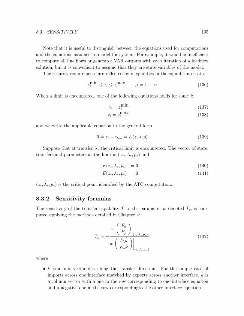
8.3. SENSITIVITY 135
Note that it is useful to distinguish between the equations used for computations
and the equations assumed to model the system. For example, it would be inefficient
to compute all line flows or generator VAR outputs with each iteration of a loadflow
solution, but it is convenient to assume that they are state variables of the model.
The security requirements are reflected by inequalities in the equilibrium states:
zmini ≤ zi ≤ zmax
i , i = 1 · · ·n (136)
When a limit is encountered, one of the following equations holds for some i:
zi = zmini (137)
zi = zmaxi (138)
and we write the applicable equation in the general form
0 = zi − zlim = E(z, λ, p) (139)
Suppose that at transfer λ∗ the critical limit is encountered. The vector of state,
transfers, and parameters at the limit is (z∗, λ∗, p∗) and
F (z∗, λ∗, p∗) = 0 (140)
E(z∗, λ∗, p∗) = 0 (141)
(z∗, λ∗, p∗) is the critical point identified by the ATC computation.
8.3.2 Sensitivity formulas
The sensitivity of the transfer capability T to the parameter p, denoted Tp, is com-
puted applying the methods detailed in Chapter 4:
Tp = −w
(FpEp
)∣∣∣∣∣(z∗,λ∗,p∗)
w
(Fλk
Eλk
)∣∣∣∣∣(z∗,λ∗,p∗)
(142)
where
• k is a unit vector describing the transfer direction. For the simple case of
imports across one interface matched by exports across another interface, k is
a column vector with a one in the row corresponding to one interface equation
and a negative one in the row corresponding to the other interface equation.

136 CHAPTER 8. SENSITIVITY OF TRANSFER CAPABILITY MARGINS
• Fp and Ep are the derivatives of the equilibrium and limit equations with respect
to parameter p.
• Fλk and Eλk are the vectors representing the derivatives of the equilibrium
and limit equations with respect to the interarea transfers in the direction of
scheduled interchange.
• w is a nonzero row vector orthogonal to the range of the Jacobian matrix J of
the equilibrium and limit equations, where
J =
(FzEz
)∣∣∣∣∣(z∗,λ∗,p∗)
(143)
The row vector w is found by solving the linear system
wJ = 0 (144)
The Jacobian matrix J has n columns and n+1 rows. Since every set of n+1 vectors
in Rn is linearly dependent, there is always a nonzero vector w that solves (144).
J generically has rank n, so that w is unique up to a scalar multiple. This scalar
multiple does not affect (142).
The first order estimate of the change in transfer capability corresponding to the
change in p of ∆p is
∆T = Tp∆p (145)
The estimate of the transfers at the critical limit for a change in p is
λ∗(p) = λ0 + k∆T (146)
Note that established sensitivity methods such as outage distribution factors and
transfer distribution factors can be derived using equation (142) as shown in Chapter
4. The derivation of these sensitivities in a general framework is useful since it extends
their application to voltage and VAR limitations.
If the security limit is due to voltage collapse or oscillatory instability, slightly
different sensitivity formulas apply, and these formulas are presented in Chapter 4.
Details concerning the formulas applicable to voltage collapse are presented in Chap-
ter 5. The formulas applicable to oscillatory instability are detailed in Chapter 9.
8.4 Example
The methods are first illustrated with a 40 bus test system to motivate the important
concepts. The methods are then tested on a realistic 1500 bus model and placed in
context of the ATC evaluation.
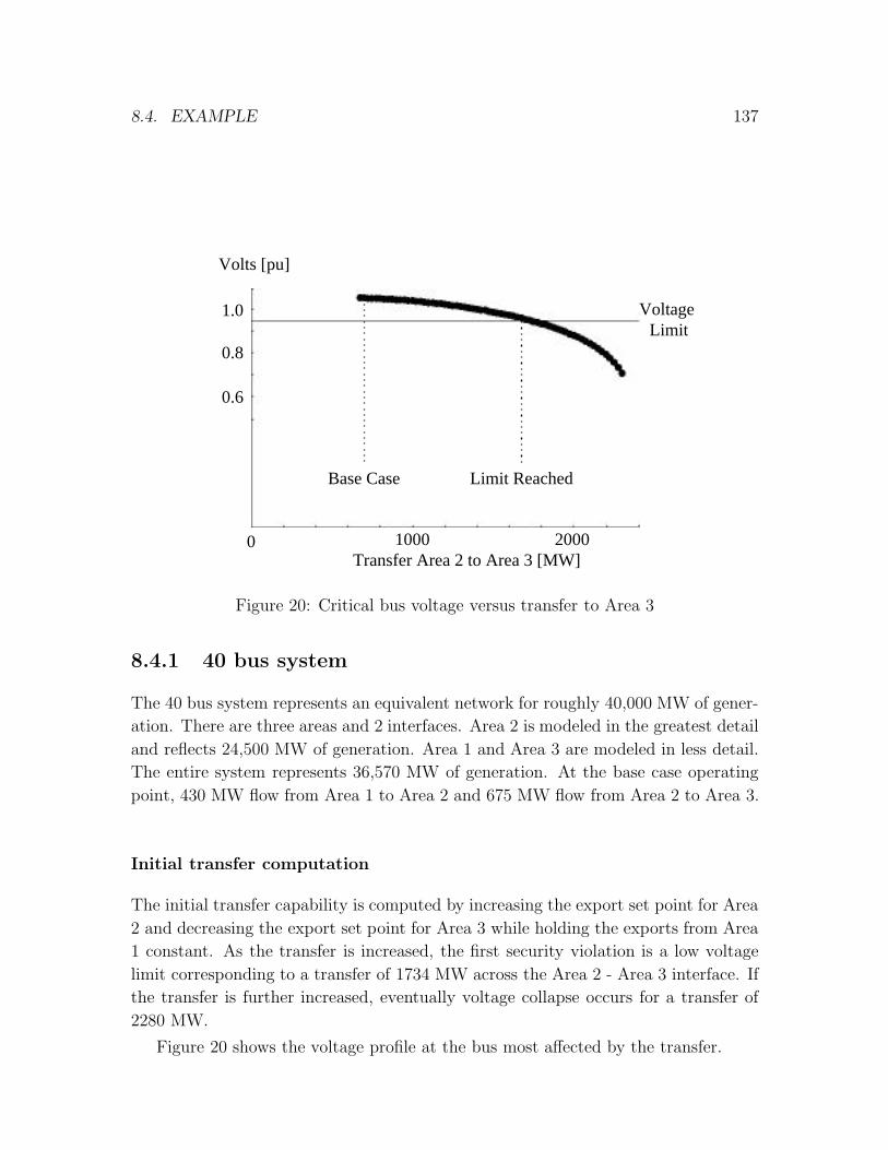
8.4. EXAMPLE 137
Transfer Area 2 to Area 3 [MW]1000 2000
0.6
Volts [pu]
0.8
1.0 Voltage Limit
0
Base Case Limit Reached
Figure 20: Critical bus voltage versus transfer to Area 3
8.4.1 40 bus system
The 40 bus system represents an equivalent network for roughly 40,000 MW of gener-
ation. There are three areas and 2 interfaces. Area 2 is modeled in the greatest detail
and reflects 24,500 MW of generation. Area 1 and Area 3 are modeled in less detail.
The entire system represents 36,570 MW of generation. At the base case operating
point, 430 MW flow from Area 1 to Area 2 and 675 MW flow from Area 2 to Area 3.
Initial transfer computation
The initial transfer capability is computed by increasing the export set point for Area
2 and decreasing the export set point for Area 3 while holding the exports from Area
1 constant. As the transfer is increased, the first security violation is a low voltage
limit corresponding to a transfer of 1734 MW across the Area 2 - Area 3 interface. If
the transfer is further increased, eventually voltage collapse occurs for a transfer of
2280 MW.
Figure 20 shows the voltage profile at the bus most affected by the transfer.

138 CHAPTER 8. SENSITIVITY OF TRANSFER CAPABILITY MARGINS
Transfer Capability
[MW]
600 800500 700200 400100 300
2000
500estimated
actual
Transfer from Area 1 [MW]
nominal
100 MW
90 MW1500
1000
2500
Figure 21: Effect of simultaneous transfer on transfer capability limited by low voltage
Simultaneous transfer
Formula (142) is evaluated to determine the sensitivity of the transfer capability
with respect to export from Area 1 at both the low voltage limit and the voltage
collapse limit. The sensitivities were used to obtain first order estimates of the transfer
capability from Area 2 to Area 3 as a function of the transfer from Area 1 to Area
2. Figure 21 shows the estimates of the transfer capability limited by the low voltage
limit and the actual computed transfer capability for a range of transfer from Area 1.
Figure 22 shows the estimates of the transfer capability limited by voltage collapse
and the actual computed transfer capability for the same range of transfer from Area
1. The dots in Figures 21 and 22 represent the actual computed boundary points
and the line represents the linear estimates. Agreement between estimates and actual
transfer capability is excellent.
Generator Dispatch
Assumptions concerning which generators back off or increase output to satisfy trans-
fers can influence the transfer capability computation. In addition, unplanned gener-
ator outages can cause previously computed transfer margins to be inaccurate.
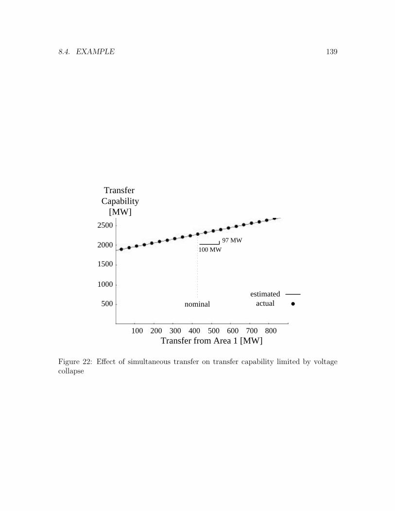
8.4. EXAMPLE 139
Transfer Capability
[MW]
600 800500 700200 400100 300
2500
500estimated
actual
Transfer from Area 1 [MW]
nominal
100 MW
97 MW
1500
1000
2000
Figure 22: Effect of simultaneous transfer on transfer capability limited by voltagecollapse
140 CHAPTER 8. SENSITIVITY OF TRANSFER CAPABILITY MARGINS
Transfer Capability
[MW]
10005000-1000
2000
500
estimatedactual
Change in Base Generation at Selected Bus [MW]
nominal
100 MW57 MW
1500
1000
2500
-500
Figure 23: Effect of generator dispatch on transfer capability limited by low voltage
The largest plant in Area 2 consists of two 1000 MW generator units. The initial
transfer computation assumed that only one unit was operational. The sensitivity
formulas were evaluated for variation of ± 1000 MW to model the effects of either
outage of the remaining unit or additional maximum output provided by the second
unit. Figure 23 compares the estimates for the resulting transfer capability with the
transfer capability computed by full continuation. Agreement is excellent over the
entire range.
Load variation
The variation of individual or aggregate loads can affect the transfer capability. Fig-
ure 24 compares the linear estimates and the actual computations of the transfer
capability resulting from changing the load level at the critical bus. The critical bus
is the bus that reached the initial low voltage limit.
Reactive power support
The sensitivity formulas could prove useful determining the effects of control actions
or planned improvements on the transfer capabilities. Figure 25 shows the effect of
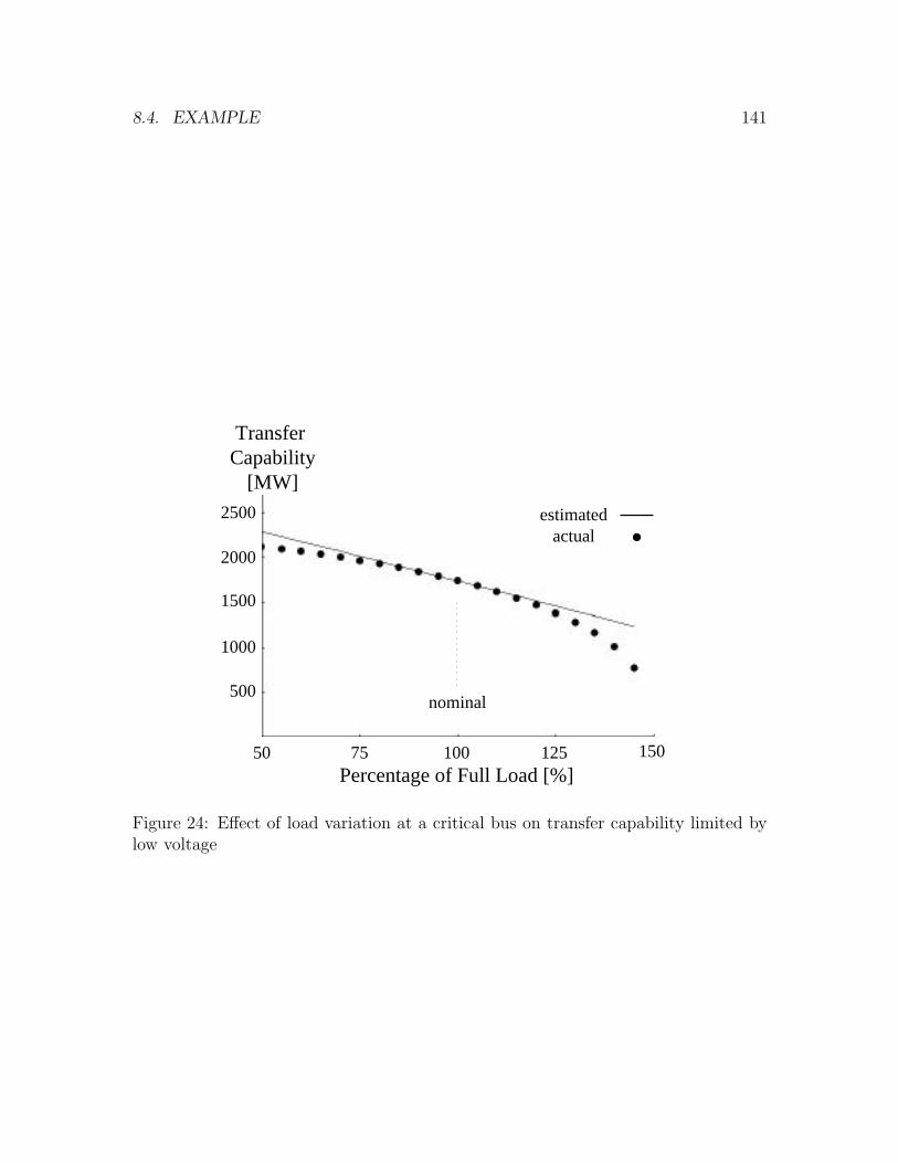
8.4. EXAMPLE 141
Transfer Capability
[MW]
15012510050
2000
500
estimatedactual
Percentage of Full Load [%]
nominal
1500
1000
2500
75
Figure 24: Effect of load variation at a critical bus on transfer capability limited bylow voltage
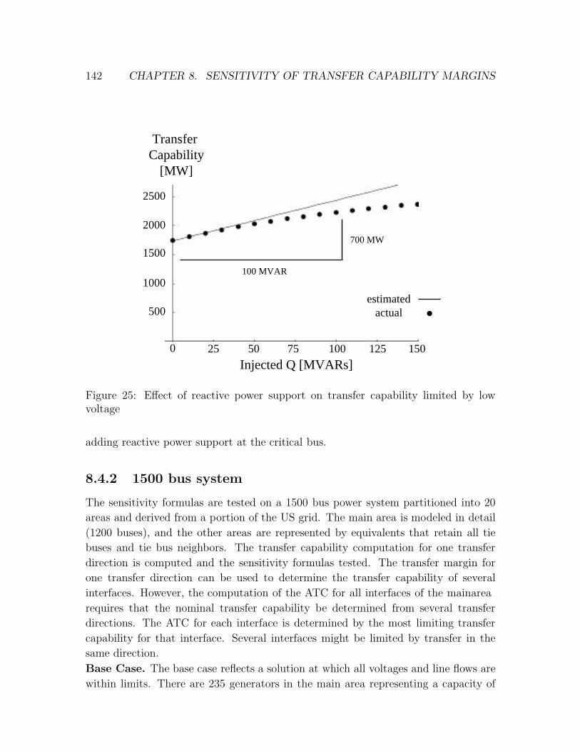
142 CHAPTER 8. SENSITIVITY OF TRANSFER CAPABILITY MARGINS
Transfer Capability
[MW]
100
estimatedactual
Injected Q [MVARs]125 1500 50 7525
2000
500
1500
1000
2500
100 MVAR
700 MW
Figure 25: Effect of reactive power support on transfer capability limited by lowvoltage
adding reactive power support at the critical bus.
8.4.2 1500 bus system
The sensitivity formulas are tested on a 1500 bus power system partitioned into 20
areas and derived from a portion of the US grid. The main area is modeled in detail
(1200 buses), and the other areas are represented by equivalents that retain all tie
buses and tie bus neighbors. The transfer capability computation for one transfer
direction is computed and the sensitivity formulas tested. The transfer margin for
one transfer direction can be used to determine the transfer capability of several
interfaces. However, the computation of the ATC for all interfaces of the main area
requires that the nominal transfer capability be determined from several transfer
directions. The ATC for each interface is determined by the most limiting transfer
capability for that interface. Several interfaces might be limited by transfer in the
same direction.
Base Case. The base case reflects a solution at which all voltages and line flows are
within limits. There are 235 generators in the main area representing a capacity of

8.4. EXAMPLE 143
Table 22: Area exports at base case, nominal transfer limit, and contingency transferlimit
Net Export Net Export Net ExportArea Base Case Flow limit Voltage LimitMain 506 MW 506 MW 506 MW
A 621 MW 1597 MW 1876 MWG -5402 MW -6378 MW -6657 MWN 1330 MW 1330 MW 1330 MW
more than 30,000 MW. The base case main area load is 24,000 MW and the total
load in the entire system is 105,000 MW. The base case existing exports for the main
area and areas A,G, and N are shown in the first column of Table 22. (Note that the
sum of these exports does not equal zero because not all areas are shown.)
The generator incremental dispatch within the main area is determined by a con-
strained economic dispatch using quadratic cost curves for each dispatchable unit.
The incremental dispatch of the other areas is assumed in proportion to the size of
each generator in that area. The assumption concerning which buses act as sources
or sinks for each transfer direction can influence the transfer capability computation.
The relative participation of individual generators depends upon the economics of
each generator. In a competitive environment utilities might be reluctant to share
data that indicates the relative profitability of each of their units.
Transfer Specification. Transfer across the Area A - Main Area interface is in-
creased by increasing import from Area A and increasing export to Area G.
Capacity Benefit Margin For this case, the CBM is selected to be twice the ca-
pacity of the largest unit in the main area. The largest unit in the main area has a
maximum output of 900 MW and the CBM is thus 1800 MW. The 1800 MW is then
allocated among six interfaces based on the results of an off-line analysis.
Transfer Reliability Margin. The critical contingency is known to be the loss of
a 500kV tie line to Area G. The transfer margin is computed for the base case as well
as the critical contingency (CITC).
Nominal and Contingency Incremental Transfer Capability The results in
this Chapter were computed using an implementation of the program described in
Chapter 3 that uses linear sensitivity to predict the next switching, MW,VAR, or flow
limit and then directly computes a full AC solution corresponding to that limiting
event. For the base case the limiting event is an overload on one 500KV line. For the
CITC computation, the limiting event is a bus voltage reaching an emergency low
voltage rating. Table 22 shows the area exports for four of the twenty areas at both
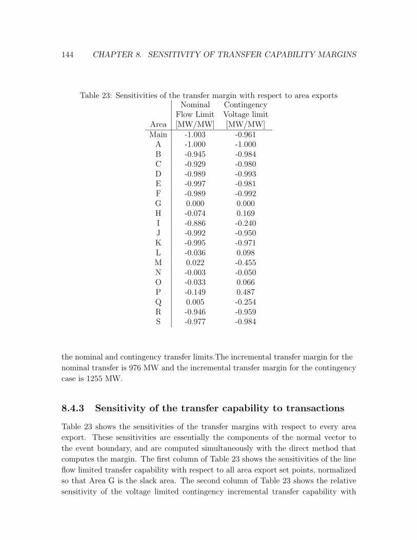
144 CHAPTER 8. SENSITIVITY OF TRANSFER CAPABILITY MARGINS
Table 23: Sensitivities of the transfer margin with respect to area exportsNominal Contingency
Flow Limit Voltage limitArea [MW/MW] [MW/MW]
Main -1.003 -0.961A -1.000 -1.000B -0.945 -0.984C -0.929 -0.980D -0.989 -0.993E -0.997 -0.981F -0.989 -0.992G 0.000 0.000H -0.074 0.169I -0.886 -0.240J -0.992 -0.950K -0.995 -0.971L -0.036 0.098M 0.022 -0.455N -0.003 -0.050O -0.033 0.066P -0.149 0.487Q 0.005 -0.254R -0.946 -0.959S -0.977 -0.984
the nominal and contingency transfer limits. The incremental transfer margin for the
nominal transfer is 976 MW and the incremental transfer margin for the contingency
case is 1255 MW.
8.4.3 Sensitivity of the transfer capability to transactions
Table 23 shows the sensitivities of the transfer margins with respect to every area
export. These sensitivities are essentially the components of the normal vector to
the event boundary, and are computed simultaneously with the direct method that
computes the margin. The first column of Table 23 shows the sensitivities of the line
flow limited transfer capability with respect to all area export set points, normalized
so that Area G is the slack area. The second column of Table 23 shows the relative
sensitivity of the voltage limited contingency incremental transfer capability with
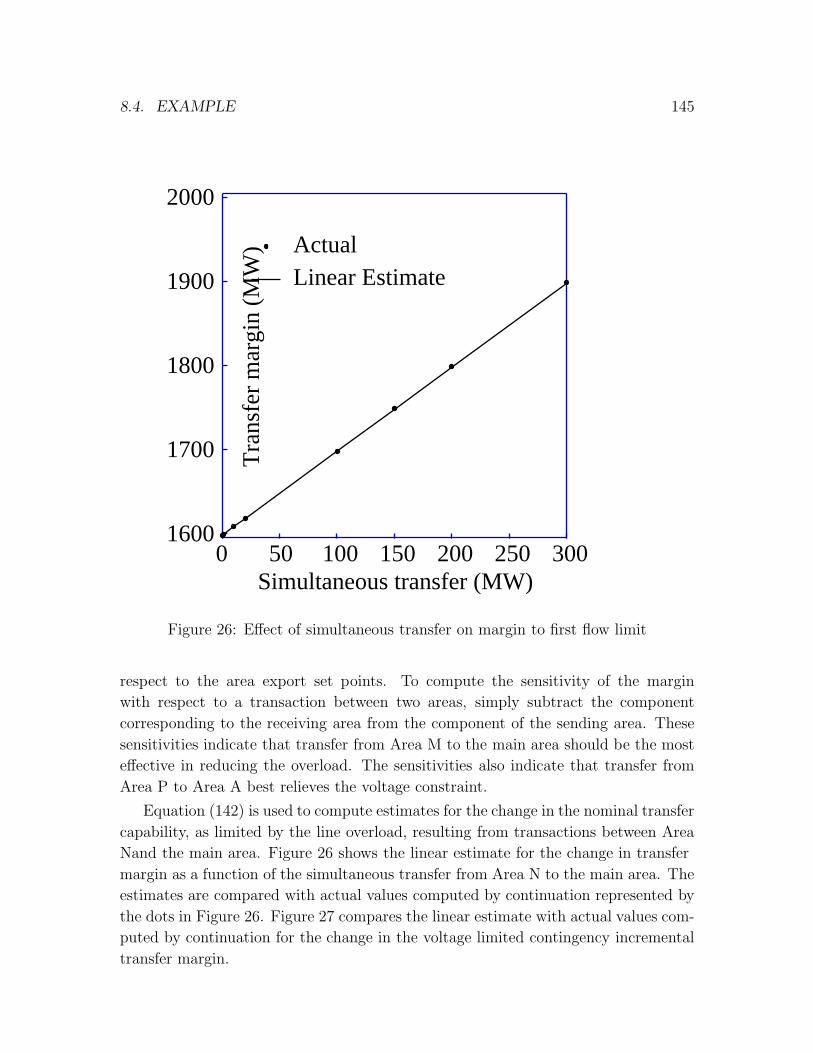
8.4. EXAMPLE 145
1600
1700
1800
1900
2000
0 50 100 150 200 250 300
ActualLinear Estimate
Tra
nsfe
r m
argi
n (M
W)
Simultaneous transfer (MW)
Figure 26: Effect of simultaneous transfer on margin to first flow limit
respect to the area export set points. To compute the sensitivity of the margin
with respect to a transaction between two areas, simply subtract the component
corresponding to the receiving area from the component of the sending area. These
sensitivities indicate that transfer from Area M to the main area should be the most
effective in reducing the overload. The sensitivities also indicate that transfer from
Area P to Area A best relieves the voltage constraint.
Equation (142) is used to compute estimates for the change in the nominal transfer
capability, as limited by the line overload, resulting from transactions between Area
N and the main area. Figure 26 shows the linear estimate for the change in transfer
margin as a function of the simultaneous transfer from Area N to the main area. The
estimates are compared with actual values computed by continuation represented by
the dots in Figure 26. Figure 27 compares the linear estimate with actual values com-
puted by continuation for the change in the voltage limited contingency incremental
transfer margin.
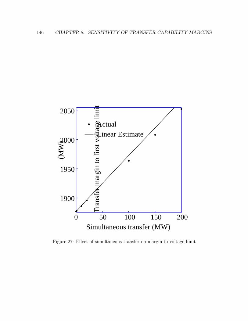
146 CHAPTER 8. SENSITIVITY OF TRANSFER CAPABILITY MARGINS
1900
1950
2000
2050
0 50 100 150 200
ActualLinear Estimate
Tra
nsfe
r m
argi
n to
fir
st v
olta
ge li
mit
(MW
)
Simultaneous transfer (MW)
Figure 27: Effect of simultaneous transfer on margin to voltage limit
8.4. EXAMPLE 147
8.4.4 Computational efficiency
Results were obtained running MATLAB version 5 uncompiled on a 200 MHz Pentium
based computer with 96 MB of RAM.
The continuation program uses exact first order sensitivities at each solved equi-
librium point to compute estimates of the transfer margins to the following events:
• generator maximum and minimum real power limits
• generator minimum reactive power limits
• line and transformer flow limits
• shunt switching events initiated by high and low voltage limits
• low bus voltage limits
Testing the program on several scenarios using the 1500 bus system indicates that
the method is effective and reduces the total number of loadflow solutions required
by each continuation. The program forces a maximum 250 MW step increase. The
average transfer step between event solutions is 120 MW, and the median step is
136 MW. The maximum step size predicted a flow limit for a 227 MW transfer with
less than a .1 MW error. 85% of solutions required 2 loadflow iterations or less
and no solutions required more than 3 iterations. (Note that in all cases maximum
transfer was limited by voltage collapse precipitated by VAR limits causing immediate
instability as indicated by the voltage sensitivity computation after application of the
limit. Direct solution of fold bifurcation solutions most likely would require more
loadflow iterations.) The mean error for the predictor step was 4.8% and the median
error was 3.7%. The majority of events are generator VAR limits and voltage limits.
Voltage and VAR limits tend to yield larger errors than real power or flow limits.
Larger step sizes were correlated with large errors.
The continuation method to establish the limiting event for a transfer direction
usually requires less than one minute. However, depending upon the initial operating
point, one continuation can take from several seconds to several minutes. From a
typical operating point, increasing the largest transfers past several limiting events to
establish the point of maximum transfer (fold bifurcation or immediate instability)
requires about 10 minutes. The method is slowed by the large number of voltage and
VAR limits that are encountered near points of extreme transfer or loading.
Computation of the event normal vector once the event point is found is about
equivalent to one iteration of the loadflow, and required less than one second. Com-
putation of the derivatives with respect to varying transfer directions is a simple index

148 CHAPTER 8. SENSITIVITY OF TRANSFER CAPABILITY MARGINS
operation requiring virtually no time once the normal vector is computed. Thus, once
the limiting event is found, the sensitivity of the transfer margin to that event with
respect to thousands of simultaneous changes in load, generation, interarea transfers
or line status can be obtained in less than one second.
8.5 Discussion
The results show that the computation of transfer margins by continuation methods
is efficient and yields important sensitivity information. The sensitivity information
is obtained as a by-product of the computation to obtain the transfer margins. The
sensitivities prove accurate at estimating the effect on the margins of simultaneous
transfer not considered by the continuation.
The example is representative of only a portion of a complete ATC computation.
The transfer margins would need to be computed for several other transfer directions.
However, the sensitivity of the margins to the area exports indicate which transfer
directions are likely to affect the margin to each event. In addition, the transfer
margins are used to determine the limiting flows on each interface. Once the in-
cremental transfer margins for enough nominal and contingency transfer directions
have been computed, the minimum flows on each interface corresponding to limiting
transfers are established. Then a portion of the CBM is allocated to each interface
and the ATC of each interface is posted for that operating horizon. The entire ATC
computation needs to be repeated for each operating horizon in which the conditions
and assumptions have changed. The practical use of accurate sensitivity information
could ease the computational burden of this process.
8.6 Conclusions and Future Work
This chapter suggests how the sensitivity of the transfer capability can be computed
and used to estimate the effect on the transfer capability of variations in parameters
such as those describing other transfers, operating conditions or assumptions. A con-
tinuation method is used to find the nominal and contingency incremental transfer
capability. The first order sensitivity of this transfer capability to a wide range of
parameters can then be quickly computed. The objective is to use these sensitivities
to quickly extract the maximum possible engineering information from each contin-
uation. The sensitivity methods could contribute to the quick update of transfer
capabilities when operating conditions or other transfers change. The sensitivity in-
formation should greatly reduce the computational burden of computing the available
transfer capability and the transfer reliability margin.
Chapter 9
Eigenvalue and margin sensitivities
for the avoidance of interarea
oscillations
The loss of system stability due to voltage collapse associated with the saddle node or
fold bifurcation was addressed in previous chapters. This chapter concerns oscillatory
instability which is associated with Hopf bifurcation. The fold bifurcation is charac-
terized by a simple zero eigenvalue of the Jacobian matrix of the system equilibrium
equations. The Hopf bifurcation is characterized by an undamped complex pair of
eigenvalues of the Jacobian matrix of the system dynamic equations. Since detec-
tion of Hopf bifurcations requires dynamic equations, not just equilibrium equations,
the analysis is different from that of the previous chapters but still follows the same
general framework.
9.1 Introduction
Interarea oscillations are often observed as oscillations of real power flow between
regions of a power system or groups of generators [IEEE1]. Voltages and current
oscillate with the power swings. If the oscillations are undamped, voltages may exceed
limits causing protective devices to trip and forcing equipment outages. Cascading
outages can lead to blackouts.
Established methods of preventing and controlling interarea oscillations require
the linearization of the system dynamic model about an operating equilibrium point
[IEEE1, Kundur, SauPai, Bergen]. The eigenvalues, and thus qualitative behavior,
of the linearized system depend upon the equilibrium point at which the system is
linearized. Standard linear control system techniques can be applied to the parameters
of the linearized model. However, when the gross operating conditions of the system
change, a new equilibrium point must be calculated and the control techniques applied
to the linearized system at that new equilibrium.
Many of the parameters that influence the system equilibrium point, such as
interarea transfers, do not appear as parameters of the linearized equations and thus
149
150 CHAPTER 9. INTERAREA OSCILLATIONS
the effects of changing these parameters on the dynamic behavior of the power system
can not be ascertained from the linearized equations. In addition, the power system
can be modeled by separate equations for different time scales. The equations that
are used to detect an oscillation (transient time scale) are different than those used
to trace the long time slow evolution of the system (steady state time scale).
This chapter presents a method for avoiding interarea oscillations by determining
the effects of controls and parameters that move the steady state system equilibrium
of the power system. The methods in this chapter can be used to analyze the effect
on an oscillation of varying interarea transfers and wheeling agreements, generator
dispatch, load shedding, and direction of load growth.
Previous Work
References [SauPai, Kundur] include both contemporary and classical approaches to
power system dynamic stability and machine modeling. The texts [WW, Bergen,
Kusic] all contain informative descriptions of the Automatic Generation Control
(AGC) and tie line bias control. The working group paper [Jal92] and its many
discussions provide an accurate assessment of current AGC practices and emphasize
the time scale appropriate for AGC. Anderson and Fouad [AF] is the classic text for
power system control and stability.
The basic mathematical analysis of the Hopf bifurcation is well covered in [GH]
and computational methods to locate Hopf bifurcations are presented in [Seydel] and
[Alv90]. Eigenvalue parametric sensitivity and generalized eigenvalue computation
is addressed in [GV]. Previous work concerning Hopf bifurcations in power systems
includes [AV84], [DAD92] and [MMH95]. [Can95] and [HH91] address saddle node
bifurcation in systems of differential-algebraic equations. Applicable work regarding
small signal stability and eigensensitivity includes [IEEE1], [Mar86], [Sme93]. [DC91]
considers the computational complexity and cost of parametric robust stability de-
termination for power system dynamic models. Methods for computing eigenvalues
and eigenvectors for power systems are presented in [Mar86, WS90, WRPK, AS96]
and for general sparse unsymmetric matrices in [DS93].
9.2 Assumptions and model
In this section we state the primary assumptions underlying the methods presented
in this chapter. The primary assumptions are implied by standard power systems
practice and are qualitative and not dependent upon specific equations for the power
system. However, secondary assumptions regarding the explicit system equations are

9.2. ASSUMPTIONS AND MODEL 151
necessary for computation and quantitative analysis.
Over transient time periods (less than one second to tens of seconds), disturbances
and fluctuating demands result in the system frequency varying about synchronous
speed. Generators respond to frequency fluctuations according to their governor
characteristics and the interarea flows vary around the scheduled transfers. The
dynamic behavior of the power system over transient time periods is assumed to be
represented by parameterized differential equations,
z = F (z, r, λ) (147)
where
F is smooth with respect to z,r and λ.
z is the vector of state variables.
r is the vector of load reference set points for each generator.
λ is a vector of parameters.
The system (147) is often modeled by a differential-algebraic system of equations
x = f(x, y, r, λ)
0 = g(x, y, r, λ)(148)
where
z = (x, y) is the vector of state variables.
f and g are smooth with respect to z,r and λ.
The derivative of g with respect to the y variables, denoted gy is nonsin-
gular evaluated over the range of interest.
The distinction between variables and parameters is crucial. Parameters are ac-
tive; they are directly set or assumed. Variables are passive; they assume the values
imposed by solution of the equations. The choice of variable and parameter is time
scale dependent. The differential-algebraic system of equations (147) account for the
transient behavior of the power system for which the vector load reference set points
is considered a parameter of (147). A perturbation to the parameters cause the state
to move from equilibrium and the system frequency to change.
The steady state behavior of the power system over longer time periods is assumed
to be represented by static equations,
0 = H(z, r, λ) (149)
where

152 CHAPTER 9. INTERAREA OSCILLATIONS
z and r are variables.
λ ∈ Rm is a vector of parameters.
H is smooth with respect to z,λ and r.
H(z0, r0, λ0) = 0 ⇒ F (z0, r0, λ0) = 0
Note that in (147) or (148) r is a parameter, but in (149) r is a variable. The equa-
tions (149) consider the time scale in which generation is economically dispatched
to meet the slowly evolving component of load fluctuation and the Automatic Gen-
eration Control (AGC) acts to maintain scheduled interchanges and restore system
frequency. Equations (147) or (148) represent the behavior of the system as the loads
and the state fluctuate about nominal equilibrium values and system frequency can
deviate from synchronous speed. Equilibria of H are equilibria of F , but H includes
equations that describe how r changes over extended periods of time to account for
economic dispatch, interarea schedules, and AGC, and assumes that system frequency
is synchronous speed.
The electrical output of a generator is controlled by two inputs, the governor droop
and the load reference set point. The governor droop determines how the generator
responds to a change in frequency. The governor droop is a constant parameter, not
a control parameter. The load reference set point determines the steady state power
output of the generator. The load reference set point is a control input that can be
revised according to an economic dispatch and permits control through the AGC.
Immediately following a disturbance the transient response of each generator is
determined by its electrical proximity to the disturbance. The system frequency a
short time (a few seconds) after a disturbance, and the proportion of the disturbance
“picked-up” by each generator, is determined by each generator’s rotating inertia.
Several seconds after a disturbance the system frequency and generator response is
affected by each generator’s governor and droop. The relative outputs of the gener-
ators when the system frequency is restored to synchronous speed is determined by
each generator’s load reference set point. The load reference set point is adjusted only
every few minutes, not seconds [Jal92]. Over transient time periods then, the load
reference is a parameter. Over longer time periods that assume steady state operation
at synchronous speed, the load reference set points are variables determined by the
system conditions and dispatch policy. At steady state the load reference set points
equal the generator power outputs.
Although the separation of the power system model into separate equations for
different time scales is not usually explicitly stated, this corresponds to the standard
practice of solving a loadflow to determine an operating point (solving (149)) but
using a detailed dynamic model (147) to either estimate the stability via eigenvalue
computation, or the transient trajectory following some disturbance. Note that the

9.2. ASSUMPTIONS AND MODEL 153
load reference set points are not always the only quantities that are a variable in
one time scale and a parameter for the other. For instance, it is common to model
loads differently for steady state time scales than for transient time scales. The key
differences between the transient and steady state models are:
• System frequency is a variable for the transient time frame and a constant for
the steady state time frame.
• Economic dispatch and area interchange occur over the steady state time frame
but not the transient time frame.
The time scale separation of the power system model is not an artifact of approx-
imate equations but a reflection of intentional control design. The decoupling of the
transient control from the operational control provides for the secure operation of the
power system during severe disturbances.
The steady state power system model is valid for some particular parameter value
λ0 if:
1. The steady state equations (149) have an equilibrium solution (z0, r0, λ0). (z0, r0)
is referred to as the equilibrium state.
2. (z0, r0) is an exponentially stable equilibrium solution of the differential equa-
tions (147).
3. The system state remains in the basin of attraction of the equilibrium solution
of the differential equations (147).
Fundamental to these assumptions is the distinction between the equilibrium state
and the system state. The system state consists of the instantaneous values of the
state variables. The equilibrium state however, is a theoretical point in state space
that represents the fixed point of the differential equations (147) that model the sys-
tem at that moment. We do not require that the power system state be at equilibrium,
only that the equations that model the system have an equilibrium.
The assumptions imply that the dynamic behavior of the power system is qual-
itatively the same as that of a linearized system at the equilibrium solution of the
differential equations (147). The stability of the power system with equilibrium state
(z0, r0) can thus be determined by the stability of the linear differential equation
z = A∆z (150)
where A = Fz|(z0,r0). Since the power system equilibrium is assumed exponentially
stable, all the eigenvalues of A have negative real part.

154 CHAPTER 9. INTERAREA OSCILLATIONS
By locating the parameters λ at which the assumptions break down, we identify
not only the limits of the model but also a boundary at which reliable operation of the
actual power system is unlikely. The model breaks down by two generic mechanisms:
1. The stable equilibrium solution disappears as parameters change.
2. The stable equilibrium solution becomes unstable as parameters change.
Mechanism (1) is characterized by the disappearance of the equilibrium solution and
is associated with voltage collapse. Mechanism (2) is characterized by a complex pair
of eigenvalues of the linearized equation (150) with zero real part corresponding to
Hopf bifurcation of the differential equations (147) and the occurrence of undamped
oscillations in the actual system. Lightly damped oscillations are problematic in the
actual power system, and correspond to eigenvalues of (150) approaching but not
necessarily crossing the imaginary axes. This chapter presents methods of predicting
and avoiding oscillations by changing λ, the parameters of the equilibrium equations
(149).
9.3 Motivation
Suppose that as a transfer increases on a power system a lightly damped mode ap-
pears. If the transfer further increases will an oscillation occur? If another transfer
is adjusted will the damping of the mode become worse or better?
One approach to answer these questions involves gathering empirical sensitivity
information from repeated computations. Several equilibrium solutions of (149) cor-
responding to different transfer levels (λ) are computed and then the eigenvalues of
(150) corresponding to each equilibrium are found. If several possible changes to the
interarea transfer are under consideration, equilibrium solutions and eigenvalues are
computed for each case. If results are needed for several different load levels, then for
each set of transfers, equilibrium and eigenvalue computations must be repeated at
each loading. This empirical sensitivity analysis is computationally burdensome.
An alternative to empirically determining sensitivity requires evaluating analyt-
ical formulas for the sensitivities of interest. In particular, we are interested in the
sensitivity of the damping of the least damped mode, and the sensitivity of the margin
to onset of oscillations (or unacceptably low damping). Instead of computing many
equilibrium solutions of (149) and corresponding eigenvalues of (150) for each, one or
only a few equilibrium solutions are obtained and the sensitivity with respect to any
parameter evaluated. The damping or margin resulting from changes to parameters
can then be approximated by a Taylor series.

9.4. COMPUTATIONS 155
The advantage of empirical sensitivity determination is accuracy. The disadvan-
tage is computing time. Analytical sensitivity evaluation offers great time savings by
many orders of magnitude.
9.4 Computations
In this section we present the formulas for the sensitivity of an eigenvalue and the
sensitivity of the margin to oscillations, with respect to any parameter.
Eigenvalue sensitivity
Assume that (z0, r0, λ0) is the present stable operating point with a lightly damped
semisimple eigenvalue µ. Let A = Fz|(z0,r0,λ0) represent the Jacobian matrix of (147)
evaluated at (z0, r0, λ0). Then an equation for µ in terms of its corresponding eigen-
vectors is
µ = wAv (151)
where w is the left (row) eigenvector of A corresponding to µ and v is the right
(column) eigenvector of A corresponding to µ. Choose w and v normalized so that
|v| = 1 and wv = 1. We are interested in how µ changes as λ varies. For instance,
λ represents the scheduled interchange transfers. As λ varies, z and r vary to satisfy
(149) and thus µ changes as A is evaluated at a different equilibrium.
µ(z, r, λ) = wFz(z, r, λ) (152)
Thus, computing the sensitivity of µ is a two step process: first the sensitivity of the
equilibrium state to changing λ is computed, and then the sensitivity of µ found by
application of the chain rule. The sensitivity of the equilibrium state with respect to
λ is found by solving the linear system
(Hz Hr
)∣∣∣o
(Zλ
Rλ
)=
(−Hλ
)∣∣∣o
(153)
where 0 = (z0, r0, λ0). The vector Zλ represents the sensitivity of the equilibrium
state with respect to λ. The vector Rλ represents the sensitivity of the load reference
set points (or mechanical inputs) to the generators with respect to λ. The sensitivity
of the eigenvalue with respect to λ is then found by evaluating
µλ =(wFzzv wFzrv
) (Zλ
Rλ
)+ wFzλv (154)
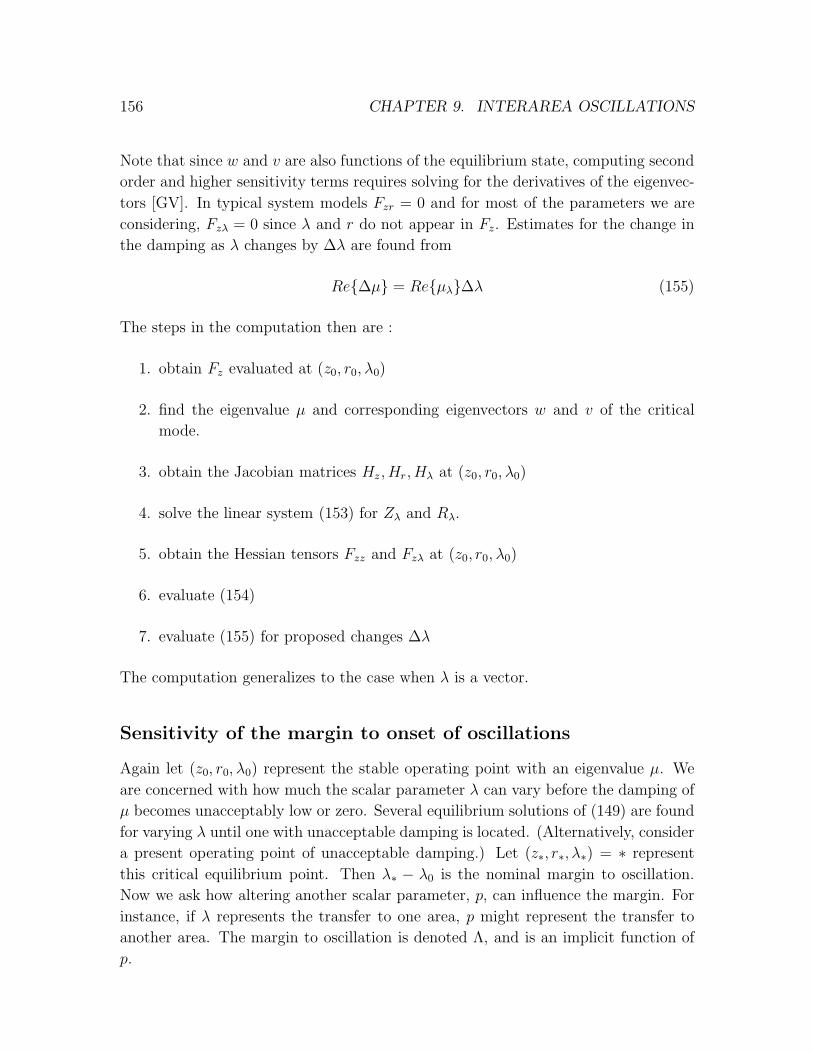
156 CHAPTER 9. INTERAREA OSCILLATIONS
Note that since w and v are also functions of the equilibrium state, computing second
order and higher sensitivity terms requires solving for the derivatives of the eigenvec-
tors [GV]. In typical system models Fzr = 0 and for most of the parameters we are
considering, Fzλ = 0 since λ and r do not appear in Fz. Estimates for the change in
the damping as λ changes by ∆λ are found from
Re{∆µ} = Re{µλ}∆λ (155)
The steps in the computation then are :
1. obtain Fz evaluated at (z0, r0, λ0)
2. find the eigenvalue µ and corresponding eigenvectors w and v of the critical
mode.
3. obtain the Jacobian matrices Hz , Hr, Hλ at (z0, r0, λ0)
4. solve the linear system (153) for Zλ and Rλ.
5. obtain the Hessian tensors Fzz and Fzλ at (z0, r0, λ0)
6. evaluate (154)
7. evaluate (155) for proposed changes ∆λ
The computation generalizes to the case when λ is a vector.
Sensitivity of the margin to onset of oscillations
Again let (z0, r0, λ0) represent the stable operating point with an eigenvalue µ. We
are concerned with how much the scalar parameter λ can vary before the damping of
µ becomes unacceptably low or zero. Several equilibrium solutions of (149) are found
for varying λ until one with unacceptable damping is located. (Alternatively, consider
a present operating point of unacceptable damping.) Let (z∗, r∗, λ∗) = ∗ represent
this critical equilibrium point. Then λ∗ − λ0 is the nominal margin to oscillation.
Now we ask how altering another scalar parameter, p, can influence the margin. For
instance, if λ represents the transfer to one area, p might represent the transfer to
another area. The margin to oscillation is denoted Λ, and is an implicit function of
p.

9.4. COMPUTATIONS 157
Computing the sensitivity of Λ with respect to p involves solving the linear system
(Hz Hr Hλ
wFzzv wFzrv wFzλv
)∣∣∣∣∣∗
Zp
Rp
Λp
=
(−Hp
−wFzpv
)∣∣∣∣∣∗
(156)
The vector (Zp, Rp) represents the sensitivity of the equilibrium state and mechanical
power inputs on the boundary of constant damping of µ as p and λ vary. Again, note
that commonly Fzλ = Fzr = Fzp = 0. Estimates for the change in the margin as p
changes by ∆p are found by
∆Λ = Λp∆p (157)
The steps in the computation are :
1. obtain the critical equilibrium (z∗, r∗, λ∗)
2. find the eigenvalue µ and corresponding eigenvectors w and v of the critical
mode at the critical equilibrium.
3. obtain the Jacobian matrices Hz , Hr, Hλ, Hp at (z∗, r∗, λ∗)
4. obtain the Hessian tensors Fzz,Fzλ and Fzp at (z∗, r∗, λ∗)
5. solve the linear system (156) for Zp,Rp, and Λp.
6. evaluate (157) for proposed changes ∆p
Solution of (156) can be simplified as follows. Compute the vector η satisfying
η
(Hz Hm
wFzzv wFzrv
)∣∣∣∣∣∗
= 0 (158)
Since
(Hz Hr
wFzzv wFzrv
)∣∣∣∣∣∗
has one more row than column, there is always a vector
satisfying (70). Pre-multiplication of equation 156 by η and rearranging yields
Λp = −η
(Hp
wFzpv
)∣∣∣∣∣∗
η
(Hλ
wFzλv
)∣∣∣∣∣∗
(159)
The sensitivity of the margin with respect to p is then found by evaluating (159).

158 CHAPTER 9. INTERAREA OSCILLATIONS
GeneratorGenerator Load
Figure 28: One line diagram of 3 bus test system
9.5 Results
This section presents results concerning measuring distances to instabilities in terms
of interarea flows, tie line flows, or flows on particular lines. Adjusting the dispatch of
generation to maintain specific line flows is one type of power system control that can
not be well represented by the classical approach of linearizing about an operating
point. Adjusting the dispatch or interchange moves the equilibrium without any
change to the parameters that appear explicitly in the linearized model.
3 bus system
The first example involves a three bus, two line system. There is a load bus connected
to two generator buses. Figure 28 shows a one line diagram of the system. From a
nominal stable operating point, increasing the load at the load bus at a constant power
factor causes a Hopf bifurcation to occur. Thus, from the stable operating point, it
is possible to measure the distance to instability with a loading margin. The loading
margin to oscillation instability can be affected by adjusting the generator dispatch.
Figure 29 shows the results for varying the proportion of load assumed by Generator
2 from 0% to 20%. The nominal percentage is assumed to be 10%. The dots represent
the actual computed bifurcation points, and the solid line is the estimate computed
by evaluating equation (157). Note that the range for which the sensitivity gives
an accurate prediction depends on the location of the nominal instability at which
computations are evaluated (Figure 30).
Eigenvalue interaction
Figures 31,32,and 33 illustrate the interaction of two complex pairs of eigenvalues
for the 3 bus power system model as the generator dispatch is varied. Each figure
corresponds to a different setting for the voltage reference set point at one of the
generator buses. Observe that a naive application of linear eigenvalue sensitivity
techniques would yield little useful information. (Imagine tangent vectors to the
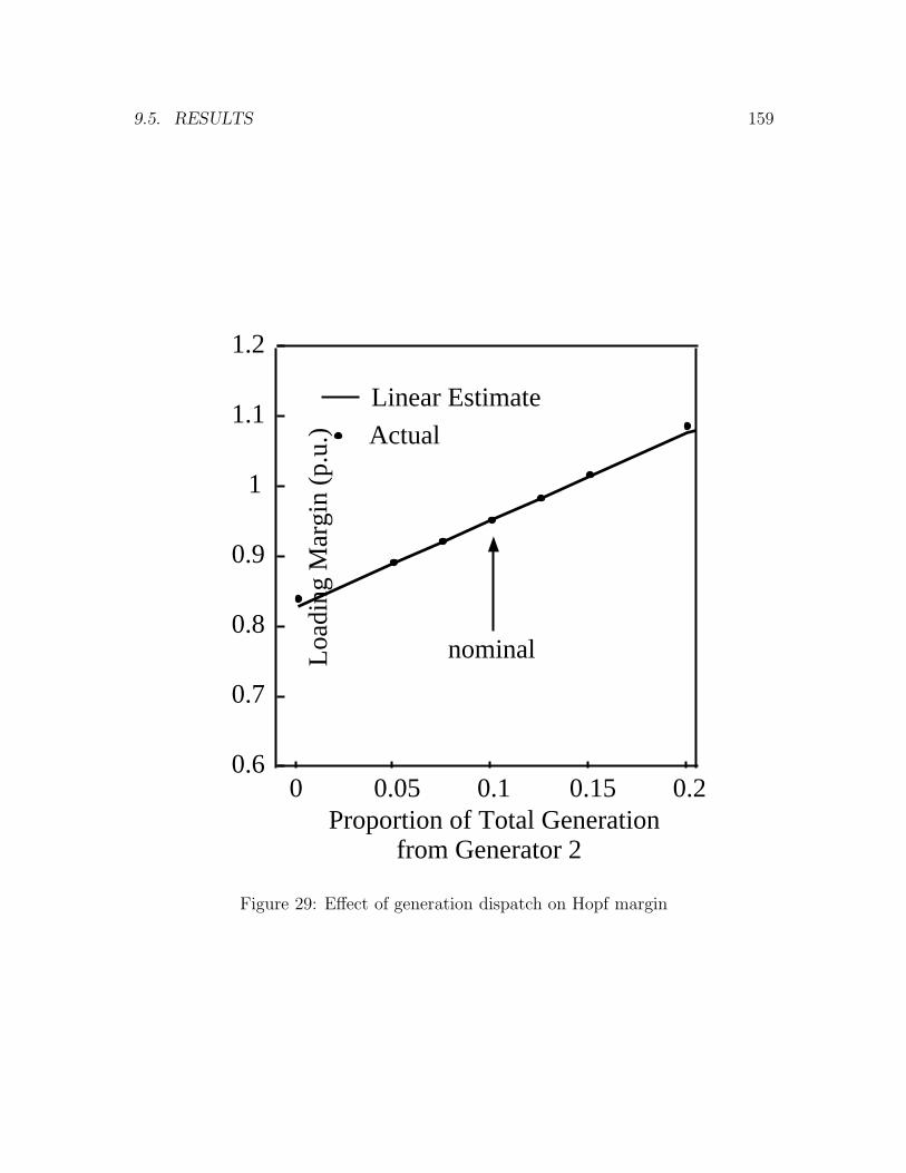
9.5. RESULTS 159
0.6
0.7
0.8
0.9
1
1.1
1.2
0 0.05 0.1 0.15 0.2
Linear Estimate
Actual
Loa
ding
Mar
gin
(p.u
.)
Proportion of Total Generationfrom Generator 2
nominal
Figure 29: Effect of generation dispatch on Hopf margin

160 CHAPTER 9. INTERAREA OSCILLATIONS
0.8
0.9
1
1.1
1.2
1.3
1.4
1.5
1.6
0 0.1 0.2 0.3 0.4 0.5 0.6
Loa
ding
Mar
gin
(p.u
.)
Proportion of Total Generationfrom Generator 2
nominal
Figure 30: Effect of generation dispatch on Hopf margin, extended variation

9.5. RESULTS 161
-4 -3 -2 -1 1 2 3 4
2
4
6
8
10 Frequency [rad/s]
Damping [s-1]
Figure 31: Trajectory of critical eigenvalues as generator dispatch is varied for gen-erator terminal voltage of 1.00 p.u.
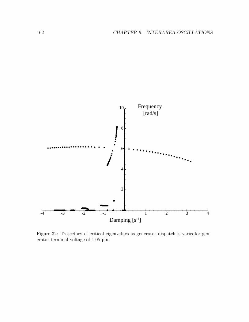
162 CHAPTER 9. INTERAREA OSCILLATIONS
-4 -3 -2 -1 1 2 3 4
2
4
6
8
10 Frequency [rad/s]
Damping [s-1]
Figure 32: Trajectory of critical eigenvalues as generator dispatch is varied for gen-erator terminal voltage of 1.05 p.u.
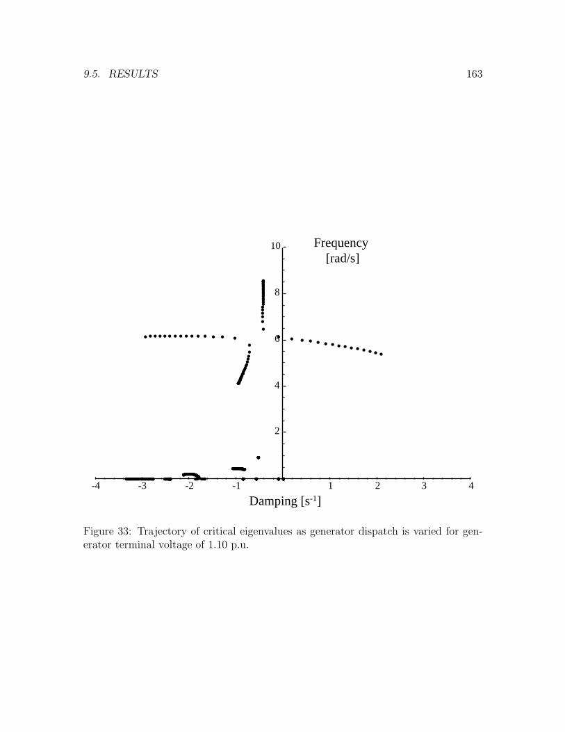
9.5. RESULTS 163
-4 -3 -2 -1 1 2 3 4
2
4
6
8
10 Frequency [rad/s]
Damping [s-1]
Figure 33: Trajectory of critical eigenvalues as generator dispatch is varied for gen-erator terminal voltage of 1.10 p.u.
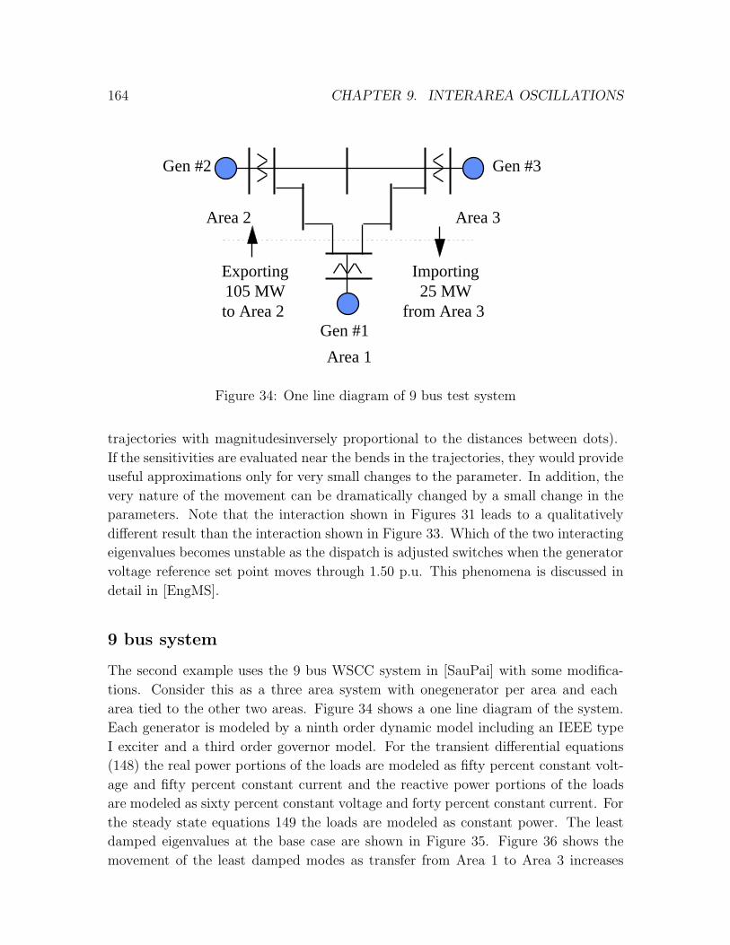
164 CHAPTER 9. INTERAREA OSCILLATIONS
Importing 25 MW
from Area 3
Gen #3Gen #2
Gen #1
Exporting 105 MW to Area 2
Area 1
Area 3Area 2
Figure 34: One line diagram of 9 bus test system
trajectories with magnitudes inversely proportional to the distances between dots).
If the sensitivities are evaluated near the bends in the trajectories, they would provide
useful approximations only for very small changes to the parameter. In addition, the
very nature of the movement can be dramatically changed by a small change in the
parameters. Note that the interaction shown in Figures 31 leads to a qualitatively
different result than the interaction shown in Figure 33. Which of the two interacting
eigenvalues becomes unstable as the dispatch is adjusted switches when the generator
voltage reference set point moves through 1.50 p.u. This phenomena is discussed in
detail in [EngMS].
9 bus system
The second example uses the 9 bus WSCC system in [SauPai] with some modifica-
tions. Consider this as a three area system with one generator per area and each
area tied to the other two areas. Figure 34 shows a one line diagram of the system.
Each generator is modeled by a ninth order dynamic model including an IEEE type
I exciter and a third order governor model. For the transient differential equations
(148) the real power portions of the loads are modeled as fifty percent constant volt-
age and fifty percent constant current and the reactive power portions of the loads
are modeled as sixty percent constant voltage and forty percent constant current. For
the steady state equations 149 the loads are modeled as constant power. The least
damped eigenvalues at the base case are shown in Figure 35. Figure 36 shows the
movement of the least damped modes as transfer from Area 1 to Area 3 increases

9.5. RESULTS 165
-1 -0.5 0
2
1
0
Frequency [Hz]
Damping [s-1]
Figure 35: Least damped eigenvalues at base case of 9 bus system.
and transfer from Area 1 to Area 2 is held constant. Figure 37 shows the movement
of the critical mode as a function of the transfer. Figure 38 shows the damping of
the critical mode as a function of the transfer and the linear estimate of the behavior
computed at the base case. We are interested in how adjusting the interchange with
one area can affect the margin to instability as measured by the interchange with an-
other area. We examine how adjusting the flow between Area 1 and Area 2 influences
the margin to instability as measured by the flow on the tie line connecting Area 1
to Area 3, and how well this behavior is predicted by the sensitivity formulas.
Figure 39 shows the effect of varying the flow between Areas 1 and 2 on the
margin to instability as measured by the flow between Areas 1 and 3. The dots are
the actual bifurcation points for each interchange; the solid line is the Taylor series
estimate computed by evaluating equation (157).
37 bus system
The 37 bus system has 3 generators represented with tenth order models and 25
generators represented with 2nd order models. Loads are considered constant power.
There are three areas represented. At the base case, Area 1 is importing about 70
MW from Area 2 and exporting about 700 MW to Area 3. As the interchange is
adjusted, generators pick up slack proportional to their size.
We are interested in the maximum amount of power that Area 1 can wheel from
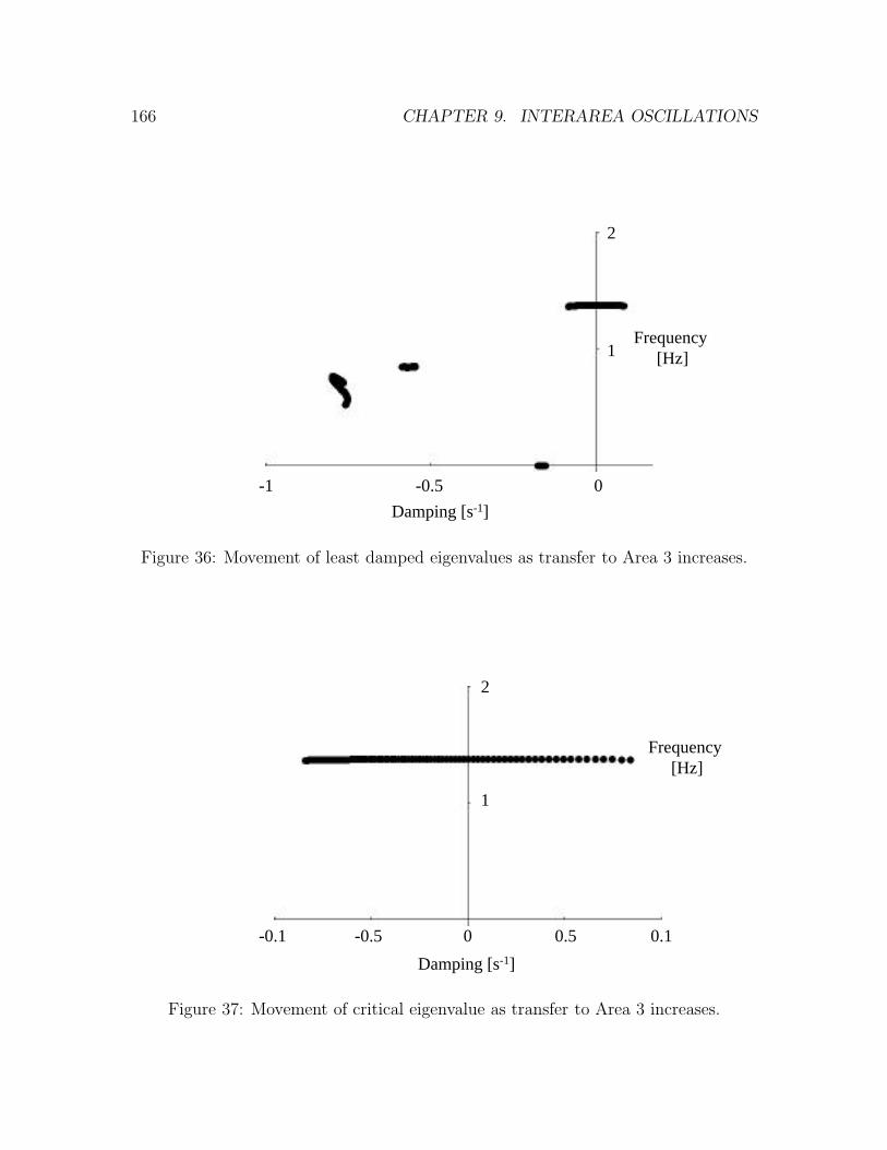
166 CHAPTER 9. INTERAREA OSCILLATIONS
-1 -0.5 0
2
1Frequency
[Hz]
Damping [s-1]
Figure 36: Movement of least damped eigenvalues as transfer to Area 3 increases.
2
1
-0.1 -0.5 0 0.5 0.1
Frequency [Hz]
Damping [s-1]
Figure 37: Movement of critical eigenvalue as transfer to Area 3 increases.

9.5. RESULTS 167
0.1
0.05
-0.1
-30 -20 -10 10 20 40 50Export[MW]
Importing 25 MWat Base Case
Damping [s-1]
Figure 38: Damping of critical mode versus linear estimate as function of transfer toArea 3 in 9 bus system.
30 40 50 60 70 80 90 100
25
50
75
110Export to Area 2 [MW]
Margin [MW]
Base Case
Figure 39: Linear estimate and actual margin to oscillations as function of export toArea 2 in 9 bus system.

168 CHAPTER 9. INTERAREA OSCILLATIONS
Area 2 to Area 3 without interarea oscillation. Eigenanalysis at the base case shows
two modes (of 80 eigenvalues) that are considerably less damped than all others.
Using the sensitivity formulas, the sensitivities of these eigenvalues are computed
with respect to the export set points for each area. These parameters appear in area
interchange equations appended to the equilibrium equations and dispatch equations.
The area interchange equations are just the sum of the real power flows on the tie lines
for each area. The area interchange parameters do not appear in the linearized small
signal equations, and hence are a prime example of the versatility of the sensitivity
formulas derived in this chapter versus classical linearization techniques that can not
account for variation of these parameters.
The computed sensitivities indicate that only one of the two modes is affected
by transfers. A succession of equilibrium points as the wheeling is increased and
decreased between zero MW and 1500 MW is computed using a continuation method
coded in Mathematica.
Figure 40 shows the damping of the sensitive eigenvalue versus the real power
wheeling. The solid line in Figure 40 represents the linear sensitivity of the damping
with respect to transfer from Area 2 to Area 3 computed at the base case. The
sensitivity computation suggests that the transfer would be limited to near 1000 MW
due to oscillation. However, the damping does not vary linearly with the transfer and
the mode never becomes unstable. If more than 1500 MW is wheeled, the system
experiences voltage stability problems.
9.6 Discussion and conclusions
This chapter illustrates the use of eigenvalue and margin sensitivities for estimating
the effects of adjusting parameters of the steady state model on the transient behavior
of the power system. These parameters, such as area export set points, do not appear
in the transient models that determine the oscillatory stability of the system and
can not be studied with traditional linearized techniques. This chapter identifies
eigenvalue interaction as a precursor to oscillatory instability. Future work could
address the possibility of avoiding oscillatory instability by detecting and controlling
eigenvalue interaction.
Several obstacles exist to successfully implementing the continuation methods to
locate Hopf bifurcations in realistic power system models. The most obvious obstacle
is computing all the eigenvalues of very large and possibly ill conditioned systems
[AS96, DS93]. This obstacle can be partially circumvented if measured data or expe-
rience can help to identify a critical mode. Possibly only one or several eigenvalues
and eigenvectors would then need to be computed and tracked. However, unlike the

9.6. DISCUSSION AND CONCLUSIONS 169
250 500 750 1000 1250 1500-0.040
-0.030
-0.020
-0.010
-0.0
Wheeling [MW]
Damping [s-1]
Figure 40: Effect of interarea exchange on damping of 37 bus system
170 CHAPTER 9. INTERAREA OSCILLATIONS
case of fold bifurcation or simple limit constraints, there is no guarantee that a lightly
damped mode will go unstable even as transfer or loading is increased. This point is
illustrated by the 37 bus system results.
Very large power system models not only contain large numbers of dynamic vari-
ables and modes, but even larger numbers of parameters, many of which are poorly
know. Even with a reduced set of important eigenvalues and a small system, eigen-
value behavior and interaction can create numerical challenges as shown by Figures
31, 32, and 33 for the three bus system. The eigenvalues of the system Jacobian ma-
trix can be sensitive to the uncertain parameters, and robust stability determination
for variation in these parameters is computationally infeasible [DC91].
9.7 Appendix
Sensitivity computations for the differential-algebraic model
Accepted practice is to model the power system with differential-algebraic equations
of the form
x = f (x, y, λ)
0 = g(x, y, λ)
Essentially, the “dynamic” variables, x, are those variables for which a differential
equation exists. For example x includes machine rotor speeds and angle deviations.
The “algebraic variables” y are those variables that do not appear explicitly as time
derivatives in the model equations. For example, the direct and quadrature axis
currents of a synchronous machine do not appear as time derivatives in the model
equations. Note that this is not to say that algebraic variables do not have dynamics,
it is simply that the time derivatives of the algebraic variables do not appear explicitly
in the equations.
For illustration, the f equations include the swing dynamics for each modeled
machine and may also include equations for voltage regulators and governor equations
for each generator. The g equations include the stator algebraic equations at each
machine as well as the power balance equations at each bus.
The distinction between algebraic and dynamic variables is a time scale separation.
The algebraic variables may be thought of as those variables with stable dynamics
much faster than those of the dynamic variables.
The parameters, λ, can include everything that is not a variable; there is no dis-
tinction between parameters that appear in the dynamic or static equations. For
example, machine moments of inertia, damping, and control gains, are parameters

9.7. APPENDIX 171
that appear in f while transmission line parameters and generator participation fac-
tors appear in g. λ may include any or all of these.
The maps f and g define another system as follows. Where the derivative of g
with respect to y is nonsingular, by the implicit function theorem there is locally a
map h such that
0 = g(x, h(x, λ), λ) (160)
The map h describes how the algebraic variables depend upon the state variables to
satisfy the algebraic constraints. We can describe the complete system then by the
composition of f with h
x = F (x, λ) = f(x, h(x, λ), λ) (161)
which is valid where h is defined. The equilibria of the system satisfy 0 = F (x, λ)
and the stability of the equilibrium (x0, λ0) is determined by the eigenvalues of the
derivative of F with respect to the state variables x. The remainder of this appendix
assumes that all derivatives are evaluated at (x0, λ0). By the Chain Rule:
Fx = fx + fyhx (162)
where hx is found from the algebraic equations.
0 = g(x, h(x), λ) ⇒ 0 = gx + gyhx ⇒ hx = −[gy]−1gx (163)
and
Fx = fx − fy[gy]−1gx (164)
There is no need to distinguish between the static and dynamic equations as
far as locating equilibrium solutions and fold bifurcations. However, detection of
the Hopf bifurcation requires attention to the Jacobian matrix Fx, not
(fx fygx gy
).
The formulas from the previous section can be applied to the eigenvalues or Hopf
bifurcation of Fx. However, computing the inverse of gy is costly. It is more intuitive
and computationally simpler to approach the problem of locating the eigenvalues of
Fx as a “generalized eigenvalue problem”.
If A and B are two square matrices of the same dimension, the pencil of A and B
is the set of all matrices that can be represented as A− µB for µ a complex number.
Each eigenvalue, µ, of the pencil satisfies
det(A− µB) = 0 (165)
and the eigenvectors corresponding to the each eigenvalue satisfy
Av = µBv (166)
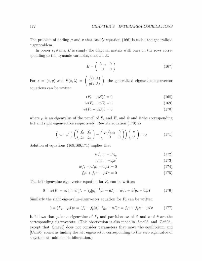
172 CHAPTER 9. INTERAREA OSCILLATIONS
The problem of finding µ and v that satisfy equation (166) is called the generalized
eigenproblem.
In power systems, B is simply the diagonal matrix with ones on the rows corre-
sponding to the dynamic variables, denoted E.
E =
(In×n 0
0 0
)(167)
For z = (x, y) and F (z, λ) =
(f (z, λ)
g(z, λ)
), the generalized eigenvalue-eigenvector
equations can be written
(Fz − µE)v = 0 (168)
w(Fz − µE) = 0 (169)
w(Fz − µE)v = 0 (170)
where µ is an eigenvalue of the pencil of Fz and E, and w and v the corresponding
left and right eigenvectors respectively. Rewrite equation (170) as
(w w′
) ((fx fygx gy
)−
(µ In×n 0
0 0
)) (v
v′
)= 0 (171)
Solution of equations (169,169,171) implies that
wfy = −w′gy (172)
gxv = −gyv′ (173)
wfx + w′gx −wµI = 0 (174)
fxv + fyv′ − µIv = 0 (175)
The left eigenvalue-eigenvector equation for Fx can be written
0 = w(Fx − µI) = w(fx − fy[gy]−1gx − µI) = wfx + w′gx − wµI (176)
Similarly the right eigenvalue-eigenvector equation for Fx can be written
0 = (Fx − µI)v = (fx − fy[gy]−1gx − µI)v = fxv + fyv
′ − µIv (177)
It follows that µ is an eigenvalue of Fx and partitions w of w and v of v are the
corresponding eigenvectors. (This observation is also made in [Sme93] and [Can95],
except that [Sme93] does not consider parameters that move the equilibrium and
[Can95] concerns finding the left eigenvector corresponding to the zero eigenvalue of
a system at saddle node bifurcation.)
9.7. APPENDIX 173
The eigenvalue sensitivity formula is found as in Chapter 4, differentiating equa-
tion (170) with respect to the parameter.
w(FzzZλ + Fzλ − µλE)v = 0 (178)
wµλEv = w(FzzZλ + Fzλ)v (179)
µλ =w(FzzZλ + Fzλ)v
wEv(180)
=w(FzzZλ + Fzλ)v
wv(181)
where Zλ is found from solution of the linear system
FzZλ = −Fλ (182)
Note that the desired normalization is still wv = 1 not wv = 1.
Computational methods for the eigenvector-eigenvalue problem can be converted
to the generalized eigenvalue approach by simply substituting the matrix µE every-
where the matrix µI is found and partitioning the eigenvectors accordingly. The for-
mulation of the eigenproblem for the differential-algebraic equations as a generalized
eigenproblem allows for the application of well established computational methods. In
addition, some routines exist specifically for generalized eigenproblems [GV, MS73].
Note that the error analysis of the generalized eigenproblem differs from that of the
standard eigenproblem. This is particularly apparent for power systems applications
that involve nearly singular gy. Although the inverse of gy does not need to be com-
puted, as gy approaches singularity the eigenvectors become very sensitive and the
sensitivity computations become poorly conditioned. This behavior can be associated
with singularity of the equilibrium equations and proximity to voltage collapse. Es-
sentially, the time scale separation implicit in constructing the differential-algebraic
model is not justified when gy approaches singularity. Future analysis is required
concerning the power system model when the algebraic variables are singular (see
[VSZ91]).

174

175
Chapter 10
Conclusions and Future Research
10.1 Conclusions
This thesis demonstrates that the computation of security margins and the sensitivity
of the security margins with respect to parameters yields practical information useful
for the control and planning of large electric power systems. The security margin
reflects the amount by which parameters can change before a security violation is
reached, and the sensitivity of that margin indicates how that margin is affected by
other parameters. The thesis establishes a coherent, consistent, and general frame-
work for margin and sensitivity analysis applicable to a variety of security criteria.
The thesis shows how to efficiently compute the security margins defined by limit-
ing events and instabilities, and the sensitivity of those margins with respect to any
model parameter.
Applications
This thesis forwards the application of margin and sensitivity methods in the areas of
voltage stability, contingency analysis, oscillatory instability, and transfer capability.
The methods of this thesis find considerable service in the area of voltage stabil-
ity and voltage collapse. The loading margin to voltage collapse is a fundamental
index of relative voltage stability and system security. We show that the sensitivity
of the loading margin to voltage collapse with respect to arbitrary parameters can be
computed efficiently and used to obtain quantitative estimates of the effects of vary-
ing parameters and assumptions. The effective use of the estimates is illustrated for
a range of system parameters including interarea transfers, load model parameters,
shunt compensation, the direction of load increase, generator dispatch, and line pa-
rameters. The closeness of the estimates over a useful range of parameter variations
and the ease of obtaining the linear estimate suggest that the sensitivity computations
will be of practical value in avoiding voltage collapse.
Generator reactive power limits have a significant influence on voltage stability and
generators reaching maximum reactive power limits can precipitate immediate voltage
collapse. The sensitivity based estimates are shown to be useful for approximating
176 CHAPTER 10. CONCLUSIONS AND FUTURE RESEARCH
the change in loading margin corresponding to changes in generator reactive power
limits. This thesis introduces the use of the normal vector to the boundary of a critical
generator reactive power limit and shows that the margin sensitivity methods work
effectively for voltage collapse caused by either saddle node bifurcation of equilibria
or immediate instability due to generator reactive power limits.
This thesis also demonstrates that effective contingency analysis for voltage col-
lapse can be done by computing the loading margin sensitivities from a single nominal
nose curve. The results show that the linear estimates are extremely fast and provide
acceptable contingency ranking. For example, after the single nose curve and a left
eigenvector are computed, the linear estimates of all single line outages for a practical
1390 bus system are computed in less time than is typically required for one load flow
solution. The quadratic estimates refine the linear estimates and are more costly but
are still faster than previous methods.
The margin and sensitivity methods are also shown to be useful for determining
transfer capabilities. Interarea transfer can be limited by several security criteria such
as low voltage limits, line flow limits, or voltage stability. The general sensitivity
formulas presented in this thesis are applicable to security margins defined by any
limit criteria. The sensitivity based estimates of the effect of simultaneous transfers
on the transfer margins are computed and agree well with the exact computations for
a 1500 bus model of a portion of the US grid. A method to compute transfer margins
by directly locating intermediate limit events reduces the total number of loadflow
iterations required by each margin computation and provides sensitivity information
for minimal additional cost.
The use of margin sensitivities for estimating the effects of adjusting steady state
model parameters on the oscillatory stability of the power system is demonstrated.
The steady state parameters such as area export set points do not appear in the
transient time scale models, but do implicitly affect the oscillatory stability. These
eigenvalue and margin sensitivities can not be computed with traditional methods
based on the linearization of the transient time scale equations. Application of the
margin and sensitivity methods to interarea oscillations has identified eigenvalue in-
teraction as a potential mechanism for instability.
Theory
This thesis extends the understanding of security margins and sensitivity computa-
tions for power systems.
This thesis defines admissible power system models based on the fundamental
assumptions of steady state analysis implied by accepted engineering practice. The
sensitivity formulas derived are valid for any power system equations that satisfy the

10.2. FUTURE WORK 177
assumptions and are independent of any approximations used to derive the equations.
It is demonstrated that the general sensitivity formulas derived in this thesis can be
reduced in special cases to yield traditional approximate sensitivity formulas such as
line distribution factors, outage distribution factors, participation factors and penalty
factors. For example, it is shown that large deviation sensitivity formulas result from
reparameterization of the system equations, that participation factors are eigenvalue
sensitivities that neglect the implicit dependence of the system Jacobian matrix on the
equilibrium point, and that exact penalty factors are the components of the normal
vector to the hypersurface in parameter space that describes how system parameters
must change to satisfy equilibrium conditions.
This thesis provides an explanation of established methods for computation of se-
curity margins synthesized from basic principles of numerical analysis. Improvements
to accepted techniques are suggested and applied. For example, by adapting the
corrector step to directly locate intermediate events of practical interest, the normal
vector to each event can be obtained at negligible cost and used to obtain sensitivities
of the security margin with respect to any parameters. In addition, the total number
of solutions required to compute the security margin are minimized.
10.2 Future work
There are several avenues for future research.
Reliability
There is growing concern over the effect of deregulation on the reliability of electric
power systems. Utilities are in need of a reliability indicator that can be tracked over
time and used to quantitatively assess system reliability. Security margins seem well
suited for this role. The loading margin to the first limit violation could be used to
compare the relative security of different systems or of the same system at different
times. In addition, the sensitivity of the reliability margin can be computed to any
parameter and used to forecast the reliability margin resulting from contingencies and
transactions.
Contingency analysis
The methods of Chapter 6 and 7 considered contingency analysis for voltage collapse
precipitated by either saddle node bifurcation of equilibria or immediate instability
due to reactive power limitations. However, the methods could be extended to any

178 CHAPTER 10. CONCLUSIONS AND FUTURE RESEARCH
security criteria or performance index. The normal vector to each event boundary
could be computed in route to establishing the nominal point of collapse, and the
contingencies ranked according to each criteria. For instance, the contingencies ranked
the highest due to their effect on the margin to voltage collapse may not be the
worst contingencies with respect to flow limits or economic cost. Chapter 6 and the
discussion to [GDA98] by Anjan Bose and Hang Liu suggest that the contingency
methods might be improved by computing more than one nominal point of collapse.
For instance, it might prove beneficial to compute the point of collapse corresponding
to different area export schedules, varying assumptions about VAR limits, or by
changing the nominal loading patterns in hopes of capturing contingencies masked
by the nominal continuation.
Constrained economic dispatch
Direct computation of the security margin and the normal vector to the event bound-
ary permits inclusion of security margin constraints in the constrained economic dis-
patch problem. Essentially, the normal vector to the boundary could be used to define
an inequality constraint in an iterative step of the optimization process. Inclusion of
security constraints in the optimization problem allows for the computation of the
components of the nodal prices attributable to reliability. This information could be
used to identify the most profitable locations to offer interruptible contracts or to
locate peaking generation.
Oscillations
Many of the difficulties encountered applying margin sensitivity methods to the prob-
lem of oscillatory instability were attributable to the large number of states repre-
sented by even modest sized power system models. In addition, the behavior of
eigenvalues is notoriously complicated. The possibility of avoiding oscillatory insta-
bility by detecting and controlling eigenvalue interaction should be investigated. One
goal for future research in the area of power system oscillations is the development of
fundamental understanding and heuristic rules for avoiding oscillations. The eigen-
value sensitivity formulas coupled with conjectures regarding power system behavior
may lead to general rules for avoiding oscillations. Approximate information concern-
ing the frequency of an oscillation and the mode shape coupled with knowledge that
increasing a particular parameter always increases the equilibrium value of a partic-
ular state variable could be used to show that changing the parameter in general will
damp that oscillation. For example, if decreasing the interarea transfer between two
areas has the effect of decreasing the angle difference between two buses, and that in

10.2. FUTURE WORK 179
general the damping of an eigenvalue associated with oscillation between those two
areas increases with the decreasing angle difference, then decreasing the interarea
transfer between the two areas would be a general guideline for suppressing oscil-
lation between those two areas. It is possible that the eigenvalue and eigenvector
sensitivity formulas may indicate that only a subset of the generator equations are
required to determine interarea oscillatory modes.

180

BIBLIOGRAPHY 181
Bibliography
[AV84] E.H. Abed, P.P. Varaiya, “Nonlinear oscillations in power systems”, In-
ternational Journal of Electric Energy and Power Systems, vol. 6, no. 1,
Jan. 1984, pp. 37-43.
[AMR] R. Abraham,J.E. Marsden,T. Ratiu, Manifolds, Tensor Analysis, and Ap-
plications, Springer-Verlag, New York, 1988.
[AF] P.M. Anderson,A.A. Fouad, Power System Control and Stability, Iowa
State University Press, Ames Iowa, 1977.
[AC92] V. Ajjarapu, C. Christy, “The continuation power flow: a tool for steady
state voltage stability analysis”, IEEE Trans. Power Systems, vol.7, no.1,
Feb.1992, pp. 416-423.
[AJYB] V. Ajjarapu, N. Jain, Z. Yu, S. Battula “Recent developments to the
continuation power flow”, Proceedings 1993 North American Power Sym-
posium, Washington D.C., Oct. 11-12, 1993, pp. 205-214.
[ABH82] F. Albuyeh, A. Bose, B. Heath, “Reactive power considerations in au-
tomatic contingency selection”, IEEE Trans. Power Apparatus and Sys-
tems, vol PAS-101, no. 1, Jan. 1982, pp. 107-111.
[AST83] O. Alsac, B. Stott, W.F. Tinney, Sparsity oriented compensation meth-
ods for modified network solutions, IEEE Trans. Power Apparatus and
Systems, vol. PAS-102, May 1983, pp. 1050-1060.
[Alv78] F. L. Alvarado, “Penalty factors from Newton’s method”, IEEE
Trans. Power Apparatus and Systems, vol. PAS-97, no. 6, Nov/Dec 1978,
pp. 2031-2040.
[Alv90] F. Alvarado, “Bifurcations in nonlinear systems: computational issues”,
Proceedings of the 1990 IEEE/ISCAS, New Orleans LA, May 1-3, 1990,
IEEE publication CH2868-8, Vol. 2, pp. 1268-1271.
[Alv97] F. L. Alvarado, “Matrix enlarging methods and their application”, BIT,
vol. 37, no. 3, 1997, pp. 473-505.
182 BIBLIOGRAPHY
[Alv91] F. Alvarado et al., “Engineering foundations for the determination of
security costs”, IEEE Trans. Power Systems, vol. 6, no. 3, Aug. 1991,
pp. 1175-1182.
[ADH94] F. Alvarado, I. Dobson, Yi Hu, “Computation of closest bifurcations in
power systems”, IEEE Trans. Power Systems, vol. 9, no. 2, May 1994, pp.
918-928.
[AJ89] F.L. Alvarado, T.H. Jung, “Direct detection of voltage collapse condi-
tions”, Proceedings: Bulk Power System Voltage Phenomena – Voltage
Stability and Security, EPRI-6183, Jan. 1989, pp. 523-538.
[Alv90] F.L. Alvarado, “Manipulation and visualization of sparse matrices”,
ORSA (Operations Research Society of America) Journal on Computing,
2(2):186-207, Spring 1990.
[AlvPhD] F.L. Alvarado, Optimal planning of power systems, PhD Thesis, Univer-
sity of Michigan, 1972.
[SMMS] Sparse Matrix Manipulation System : Users manual and software available
via anonymous ftp at eceserv0.ece.wisc.edu in subdirectory pub/smms93
[AS96] G. Angelidis, A. Semlyen, “Improved methodologies for the calculation of
critical eigenvalues in small signal stability analysis”, IEEE Trans. Power
Systems, vol. 11, no. 3, Aug 1996, pp. 1209-1217.
[Bergen] A.R. Bergen, Power Systems Analysis, Prentice-Hall, Englewood Cliffs
NJ, 1986.
[BN] F. Brauer, J. Nohel, The Qualitative Theory of Ordinary Differential
Equations, Dover, NY, 1969.
[CA93] C.A. Canizares, F.L. Alvarado, “Point of collapse and continuation meth-
ods for large AC/DC systems”, IEEE Trans. Power Systems, vol.7, no.1,
Feb.1993, pp. 1-8.
[CA91] C.A. Canizares, F.L. Alvarado, “Computational experience with the point
of collapse method on very large AC/DC systems”, in [DCL].
[Can98] C.A. Canizares, “Calculating optimal system parameters to maximize the
distance to saddle-node bifurcations”, IEEE Trans. Circuits and Systems
— I:Fundamental Theory and Applications, vol. 45, no. 3, March 1998,
pp.225-237.

BIBLIOGRAPHY 183
[Can95] C.A. Canizares, “Conditions for saddle-node bifurcations in AC/DC
power systems”, Electrical Power & Energy Systems, vol.17, no.1, 1995,
pp. 61-68.
[CanPhD] C.A. Canizares, Voltage Collapse and Transient Energy Function Analy-
ses of AC/DC Systems, PhD. Thesis, University of Wisconsin–Madison,
1991.
[PFLOW] PFLOW : Software available via anonymous ftp at iliniza.uwaterloo.ca in
subdirectory pub/pflow
[CFSB] H.-D. Chiang, A. Flueck, K.S. Shah, N. Balu, “CPFLOW: A practical
tool for tracing power system steady-state stationary behavior due to
load and generation variations”, IEEE Trans. Power Systems, vol. 10, no.
2, May 1995, pp. 623-634.
[CWF97] H-D Chiang, C-S Wang, A.J. Flueck, “Look-ahead voltage and load mar-
gin contingency selection functions for Large-Scale Power Systems”, vol.
12, no. 1, Feb. 1997, pp. 173-180.
[CH] S.N. Chow, J. Hale, Methods of bifurcation theory, section 6.2, Springer
Verlag, NY, 1982.
[CA95] M. L.Crow, J. Ayyagari, “The effect of excitation limits on voltage sta-
bility”, IEEE Trans. Circuits and Systems — I:Fundamental Theory and
Applications, vol. 42, no. 12, Dec. 1995, pp. 1022-1026.
[Davos] L.H. Fink, ed., Proceedings: Bulk power system voltage phenomena III,
voltage stability, security & control, ECC/NSF workshop, Davos, Switzer-
land, Aug. 1994.
[DCL] L.H. Fink, ed., Proceedings: Bulk power system voltage phenomena, volt-
age stability and security, ECC/NSF workshop, Deep Creek Lake, MD,
Aug. 1991, ECC Inc., 4400 Fair Lakes Court, Fairfax, VA 22033-3899.
[Debs] A.S. Debs, Modern Power Systems Control and Operation, Kluwer Aca-
demic, Boston, 1988.
[DV93] C. L. DeMarco, G. C. Verghese, “Bringing phasor dynamics into the power
system load flow”, Proceedings 1993 North American Power Symposium,
Washington D.C., Oct. 11-12, 1993, pp. 463-471.
184 BIBLIOGRAPHY
[DeM96] C. L. DeMarco, “A novel continuation method for computing alternate
power flow solutions”, Proceedings 1996 North American Power Sympo-
sium, Cambridge, MA, Nov. 1996.
[DC91] C. L. DeMarco, G. E. Coxson, “Computational complexity results in para-
metric robust stability analysis with power system applications”, in Sys-
tems and Control Theory for Power Systems, Springer-Verlag, NY, 1991.
[DS93] J. Deuse, M. Stubbe, “Dynamic simulation of voltage collapses, IEEE
Trans. Power Systems, vol.8, no.3, Aug.1993, pp. 894-904.
[DAD92] I. Dobson, Fernando Alvarado and C. L. DeMarco, “Sensitivity of Hopf
bifurcations to power system parameters”, Proceedings of the 31st Confer-
ence on Decision and Control, Tucson, Arizona, Dec. 1992, pp. 2928-2933.
[DC89] I. Dobson, H.-D. Chiang, “Towards a theory of voltage collapse in electric
power systems, Systems and Control Letters, vol. 13, 1989, pp. 253-262.
[Dob94] I. Dobson, “The irrelevance of load dynamics for the loading margin to
voltage collapse and its sensitivities”, in [Davos].
[Dob92] I. Dobson, “Observations on the geometry of saddle node bifurcation and
voltage collapse in electric power systems”, IEEE Trans.Circuits & Sys-
tems,Part 1, vol.39, no.3, Mar.1992, pp. 240-243.
[Dob93] I. Dobson, “Computing a closest bifurcation instability in multidimen-
sional parameter space”, Journal of Nonlinear Science, vol. 3, no. 3, 1993,
pp. 307-327.
[DL192] I. Dobson, L. Lu, “Computing an optimum direction in control space
to avoid saddle node bifurcation and voltage collapse in electric power
systems”, IEEE Trans. Automatic Control, vol 37, no. 10, Oct. 1992, pp.
1616-1620.
[DL292] I. Dobson, L. Lu, “Voltage collapse precipitated by the immediate change
in stability when generator reactive power limits are encountered”, IEEE
Trans. Circuits and Systems, Part 1, vol. 39, no. 9, Sept. 1992, pp. 762-
766.
[DL93] I. Dobson, L. Lu, “New methods for computing a closest saddle node
bifurcation and worst case load power margin for voltage collapse”, IEEE
Trans. Power Systems, vol.8, no.3, Aug.1993, pp. 905-913.
BIBLIOGRAPHY 185
[DT68] H. W. Dommel,W. F. Tinney, “Optimal power flow solutions”, IEEE
Trans. on Power Apparatus and Systems, vol. PAS-87, no.3, Oct. 1968,
pp. 1866-1876.
[DGM79] R. D. Dunlop, R. Gutman and P. P. Marchenko, “Analytical Develop-
ment of Loadability Characteristics for EHV and UHV Transmission
Lines,” IEEE Trans. Power Apparatus and Systems, Vol. PAS-98, No.
2, March/April 1979, pp. 606-617.
[DS93] I. S. Duff, J. A. Scott, “Computing selected eigenvalues of sparse unsym-
metric matrices using subspace iteration”, ACM Transactions on Mathe-
matical Software, vol. 19, No. 2, June 1993.
[EngMS] H. Engdahl, Simulation eveidence for interacting pairs of eigenvalues caus-
ing oscillations in electric power systems, MS. Thesis, Royal Institute of
Technolgy, Stockholm,1998.
[EVMW] G.C. Ejebe, H.P. Van Meeteren, B.F. Wollenberg, “Fast contin-
gency screening and evaluation for voltage security analysis”, IEEE
Trans. Power Systems, vol. 3, no. 4, Nov. 1988, pp. 1582-1590.
[EIMORT] G.C. Ejebe, G.D. Irisarri, S. Mokhtari, O. Obadina, P. Ristanovic, J.
Tong, “Methods for contingency screening and ranking for voltage stabil-
ity analysis of power systems”, IEEE Trans. Power Systems, vol. 11, no.
1, Feb. 1996, pp. 350-356.
[ECSW] A.O. Ekwue, D.T.Y. Cheng, Y.H. Song, H.B. Wan, “Integrated methods
for voltage stability analysis of the NGC system”, Colloquium on Voltage
Collapse, Digest No. 1997/101 Institution of Electrical Engineers, London,
UK.
[PSerc] P. Sauer, M.A. Pai, S. Fernandes, I. Dobson, F. Alvarado, S. Greene, B.
Thomas, H-D Chiang, “Real time control of oscillations of electric power
systems”, ESEERCO Project EP 95-11, Sep. 1996.
[FOC90] N. Flatabø, R. Ognedal, T. Carlsen, “Voltage stability condition in a
power transmission system calculated by sensitivity methods”, IEEE
Trans. Power Systems, vol. 5, no. 4, Nov. 1990, pp. 1286-1293.
[FFOCH] N. Flatabø, O.B. Fosso, R. Ognedal, T. Carlsen, K.R. Heggland, “A
method for calculation of margins to voltage instability applied on
the Norwegian system for maintaining required security level”, IEEE
Trans. Power Systems, vol. 8, no. 2, May 1993, pp. 920-928.

186 BIBLIOGRAPHY
[FCW97] A.J. Flueck, H-D. Chiang, C-S. Wang, “A novel method of look-ahead
contingency ranking for saddle-node bifurcation”, Proceedings of the
20th International Conference on Poweer Industry Computer Applica-
tions 1997, Columbus, Ohio, May 11-16, 1997 pp. 266-271.
[FFHH] O.B. Fosso, N. Flatabø, B. Hakavik, A.T. Holen, “Comparison of meth-
ods for calculation of margins to voltage instability”, Proceedings Athens
Power Tech 1993, Athens, Greece, Sep. 5-8, 1993, pp. 216-221.
[Gal84] F.D. Galiana, “Bound estimates of the severity of line outages in power
system contingency analysis and ranking”, IEEE Trans. Power Apparatus
and Systems, vol PAS-103, no. 9, Sep. 1984, pp. 2612-2624.
[GZ] C.B. Garcia, W.I. Zangwill, Pathways to Solutions, Fixed Points, and
Equilibria, Prentice-Hall, Englewood Cliffs NJ, 1983.
[GVHW] L. L. Garver, P. R. Van Horne and K. A. Wirgau, “Load Supplying Ca-
pability of Generation-Transmission Networks,” IEEE Trans. Power Ap-
paratus and Systems, Vol. PAS-98, No. 3, May/June 1979, pp. 957-962.
[GV] G. Golub, C. VanLoan, Matrix Computations, Johns Hopkins Universtiy
Press, Baltimore, 1983.
[GSHT] P.R. Gribik, D. Shirmohammadi, S. Hao, C.L. Thomas, “Optimal power
flow sensitivity analysis”, IEEE Trans. Power Systems, vol. 6, no. 2, May
1991, pp. 969-976.
[GDA97] S. Greene, I. Dobson, F.L. Alvarado, “Sensitivity of the loading mar-
gin to voltage collapse with respect to arbitrary parameters”, IEEE
Trans. Power Systems, vol. 12, no. 1, Feb. 1997, pp. 262-272.
[GDA98] S. Greene, I. Dobson, F.L. Alvarado, “Contingency analysis for voltage
collapse via sensitivities from a single nose curve”, paper PE-707-PWRS-
2-06-1997,IEEE PES Summer Meeting, Berlin, Germany, July 1997.
[GDAS] S. Greene, I. Dobson, F.L. Alvarado, P.W. Sauer, Initial concepts for
applying sensitivity to transfer capability, NSF Workshop on Available
Transfer Capability, Urbana IL USA, June 1997.
[GreMS] S. Greene, Constraint at a saddle node bifurcation, MS thesis, Univ. of
Wisconsin-Madison, 1993.
BIBLIOGRAPHY 187
[GH] J. Guckenheimer, P. Holmes, Nonlinear Oscillations, Dynamical Systems,
and Bifurcations of Vector Fields, Springer-Verlag, NY, 1983.
[GP] V. Guillemin, A. Pollack, Differential Topology, Prentice-Hall, Englewood
Cliffs NJ, 1974.
[HSS] N. T. Hawkins, G. Shackshaft, M.J. Short, “On-line algorithms for the
avoidance of voltage collapse: reactive power management and voltage
collapse margin assessment”, Proceedings of the IEE Third International
Conference on Power System Monitoring and Control, Institution of Elec-
trical Engineers, London, 1991, pp. 134-139.
[HawPhD] N. T. Hawkins “On-line reactive power management in electric power
systems”, PhD thesis, University of London, Department of Electrical
and Electronic Engineering, Imperial College of Science, Technology, and
Medicine, London, 1996
[Heydt] Heydt, Computer Analysis Methods for Power Systems, Macmillan Pub-
lishing Company, NY, 1986.
[HD95] I. Hiskens, R. J. Davy “A technique for exploring the power flow solution
space boundary”, Proceedings Stockholm Power Tech, Stockholm, June
18-22, 1995 , pp. 478-483.
[HH91] I. Hiskens, D. Hill, “Dynamic aspects of voltage collapse”, in [DCL].
[HJ] R.A. Horn, C.R. Johnson, Matrix Analysis, Cambridge University Press,
Cambridge, 1985.
[Iba] K. Iba et al., “Calculation of critical loading condition with nose curve
using homotopy continuation method”, IEEE Trans. Power Systems, vol.
6, May 1991, pp. 584-593.
[IEEE1] Inter-Area Oscillations in Power Systems, IEEE Special Publication 95-
TP-101, 1995.
[IEEE1] Voltage stability of power systems: concepts, analytical tools, and indus-
try experience, IEEE Special Publication 90TH0358-2-PWR, 1990.
[IEEE3] Recommended techniques for voltage stability analysis, Working Group
on Voltage Stability, System Dynamic Performance Subcommittee IEEE
Special Publication, 1994.

188 BIBLIOGRAPHY
[Jal92] N. Jaleeli, et. al., “Understanding automatic generation control”, IEEE
Transactions on Power Systems, vol. 7, no. 3, Aug. 1992, pp. 1106-1122.
[JJC92] R. Jean-Jumeau, H.D. Chiang, “Parameterizations of the load-flow
equations for eliminating ill-conditioning load flow solutions”, IEEE
Trans. Power Systems, vol. 8, no. 3, Aug. 1995, pp. 1004-1012.
[Kundur] P. Kundur, Power System Stability and Control, McGraw-Hill, NY, 1993.
[Kur93] A. Kurita et al.,“ Multiple time-scale power system dynamic simulation”,
IEEE Trans. Power Systems, vol. 8, no. 1, Feb. 1993, pp. 216-223.
[Kusic] G.L. Kusic, Computer-Aided Power Systems Analysis, Prentice-Hall, En-
glewood Cliffs, NJ, 1986.
[Kwa86] H. G. Kwatny, et al., “Static bifurcation in electric power networks: loss
of steady state stability and voltage collapse”, IEEE Trans. on Circuit
and Systems, vol. CAS-33, no. 10 Oct. 1986, pp. 981-991.
[LTA72] G. L. Landgren, H. L. Terhune, R. K. Angel, “Transmission Interchange
Capability - Analysis by Computer,” IEEE Trans. Power Apparatus and
Systems, Vol. PAS-91, No. 6, Nov/Dec 1972, pp. 2405-2414.
[LA73] G. L. Landgren, S. W. Anderson, “Simultaneous Power Interchange Ca-
pability Analysis,” IEEE Trans. Power Apparatus and Systems, Vol. PAS-
92, No. 6, Nov/Dec 1973, pp. 1973-1986.
[LAH95] P.A. Lof,G. Andersson, D. Hill, “Voltage dependent reactive power limits
for voltage stability studies”, IEEE Trans. Power Systems, vol. 10, no. 1,
Feb. 1995, pp. 220-228.
[LofPhD] Per-Anders Lof, Steady-State Stability Analysis, PhD Thesis, Royal Insti-
tute of Technology, Stockholm, TRITA-EES-9501, ISSN 1100-1607, 1995.
[LLT94] J. Lu, C-W Liu, J. S. Thorp, “New methods for computing a saddle-
node bifurcation point for voltage stability analysis”, IEEE Trans. Power
Systems, vol. 10, no. 2, May 1995, pp. 978-985.
[MMH95] Y.V. Makarov, V. A. Maslennikov, D.J. Hill, “Calculation of oscillatory
stability margins in the space of power system controlled parameters”,
Proceedings Stockholm Power Tech, Stockholm, June 18-22, 1995, pp.
416-421.

BIBLIOGRAPHY 189
[MMH96] Y.V. Makarov, V. A. Maslennikov, D.J. Hill, “Revealing loads having
the biggest influence on power system small disturbance stability”, IEEE
Trans. Power Systems, vol. 11, no. 4, Nov. 1996, pp. 2018-2023.
[MATLAB] MATLAB : The Math Works, Inc. , Natick MA.
[Mar86] N. Martins, “Efficient eigenvalue and frequency response methods applied
to power system small-signal stability studies”, IEEE Transactions on
Power Systems, vol. PWRS-1, no. 1, 1986, pp. 217-226.
[MS73] C.B. Moler, G.W. Stewart, “An algorithm for generalized matrix eigen-
value problems, SIAM Journal of Numerical Analysis, 10, 1973, pp. 241–
256.
[MTK96] H. Mori, H. Tanaka, J. Kanno, “A preconditioned fast decoupled power
flow method for contingency screening”, IEEE Trans. Power Systems, vol.
11, no. 1, Feb. 1996, pp. 357-363.
[NTSCO] K.Nara, K. Tanaka, R.R. Shoults, M.S. Chen, P. Van Olinda, “On-
line contingency selection algorithm for voltage security analysis”, IEEE
Trans. Power Apparatus and Systems, vol PAS-104, no. 4, April 1985, pp.
847-856.
[NERC95] Transmission Transfer Capability Task Force, “Transmission transfer ca-
pability”, North American Reliability Council, Princeton, New Jersey,
May 1995.
[NERC96] Transmission Transfer Capability Task Force, “Available transmission
capability definitions and determination”, North American Reliability
Council, Princeton, New Jersey, June 1996.
[NorPhD] M. Noroozian, Exploring benefits of controllable series compensators in
power systems, PhD Thesis, Royal Institute of Technology, Stockholm,
TRITA-EES-9402, ISSN 1100-1607, 1994.
[OloPhD] M. Olofsson, Optimal operation of the Swedish railway electrical sys-
tem, PhD Thesis, Royal Institute of Technology, Stockholm, TRITA-EES-
9601, ISSN 1100-1607, 1996.
[OD91] T.J. Overbye, C.L. DeMarco, “Voltage security enhancement using energy
based sensitivities”, IEEE Trans. Power Systems, vol. 6, no. 3, Aug. 1991,
pp. 1196–1202.

190 BIBLIOGRAPHY
[PPAV] F. L. Pagola, I. J. Perez-Arriaga and G. C. Verghese, “On sensitivities,
residues and participants: Applications to oscillatory stability analysis
and control,” IEEE Transactions on Power Systems, vol. PWRS-4, no. 1,
1989, pp. 278-285.
[PAVS] I. J. Perez-Arriaga, G. C. Verghese and F. C. Scheweppe, “Selective modal
analysis with applicatons to electric power systems, Part I and II,” IEEE
Transactions on Power Apparatus and Systems, vol. PAS 101, no. 9, 1982,
pp. 3117-3134.
[PPTT] J. Peschon, D. S. Percy, W. F. Tinney, O.J. Tveit, “Sensitivity in power
systems”, IEEE Trans. Power Apparatus and Systems, vol PAS-87, no. 8,
Aug. 1968, pp. 1687-1696.
[RHSC] C. Rajagopalan, S. Hao, D. Shirmohammadi, M.K. Celik, “Voltage col-
lapse operating margin analysis using sensitivity techniques”, Proceedings
Athens Power Tech 1993, Athens, Greece, Sep. 5-8, 1993, pp.332-336.
[RAMCJ] R. Rajaraman, F. Alvarado, A. Maniaci, R. Camfield, S. Jalali, “Deter-
mination of location and amount of series compensation to increase power
transfer capability”, IEEE Trans. Power Systems, vol.13, no.2, May 1998,
pp. 294-300.
[Reid] J. K. Reid editor, Large Sparse Sets of Linear Equations, Proceedings of
the Oxford conference of the Institute of Mathematics and Its Applica-
tions held in April, 1970 Academic Press, London, 1971.
[RAUPG] N.D. Reppen, R.R. Austria, J.A. Uhrin, M.C. Patel,A. Galatic, “Perfor-
mance of methods for ranking and evaluation of voltage collapse contin-
gencies applied to a large-scale network”, Proceedings Athens Power Tech
1993, Athens, Greece, Sep. 5-8, 1993, pp.337-343.
[SRP91] P. W. Sauer, C. Rajagopalan and M. A. Pai, “An explanation and gen-
eralization of the AESOPS and PEALS algorithms,” IEEE Transactions
on Power Systems, vol. 6, no. 1, Feb. 1991, pp. 293-299.
[Sau97] P.W. Sauer, “Technical challenges of computing available transfer capa-
bility (ATC) in electric power systems”, 30th Hawaii International Con-
ference on System Science, Maui, Hawaii, Jan. 1997.
[SauPai] P. W. Sauer, M. A. Pai, Power System Dynamics and Stability, Prentice-
Hall, Englewood Cliffs NJ, 1996.
BIBLIOGRAPHY 191
[SenPhD] Ontoseno Penangsang, Fast linear screening approach for contingency se-
lection of line outages based on voltage quality, PhD Thesis, University
of Wisconsin–Madison, May 1983.
[Seydel] R. Seydel, From equilibrium to chaos; practical bifurcation and stability
analysis, Elsevier, NY, 1988.
[Sme93] T. Smed, “Feasible eigenvalue sensitivity for large power systems,” IEEE
Transactions on Power Systems, vol. 8, no. 2, May 1993, pp. 555-563.
[Spivak] M. Spivak, Calculus on Manifolds, Addison-Wesley, NY, 1965.
[StC53] H. P. St. Clair, “Practical Concepts in Capability and Performance of
Transmission Lines,” AIEE Transactions, Vol. 72, Part III, Dec. 1953,
pp. 1152-1157.
[Sto74] B. Stott, “Review of load flow calculation methods”, Proceedings of the
IEEE, Vol. 62, No. 1, July 1974, pp. 916-929.
[Sto79] B. Stott, “Power System Dynamic Response Calculations”, Proceedings
of the IEEE, Vol. 67, No. 2, Feb. 1979, pp. 219-241.
[SM79] B. Stott, J. L. Marinho, “Linear Programming for Power System Network
Security Applications,” IEEE Trans. on Power Apparatus and Systems,
Vol. PAS-98, No. 3, May/June 1979, pp. 837-848.
[SAA85] B. Stott, O. Alsac, F.L. Alvarado, Analytical and computational improve-
ments in performance-index ranking algorithms for networks, Interna-
tional Journal of Electrical Energy and Power Systems, vol. 7, no. 3, July
1985, pp.154-160.
[TMI83] Y. Tamura, H. Mori, S. Iwamoto, “Relationship between voltage insta-
bility and multiple load flow solutions in electric power systems” IEEE
Trans. on Power Apparatus and Systems, Vol. PAS-102, no. 5, May 1983,
pp. 1115-1125.
[TT88] A. Tiranuchit, R.J. Thomas, “A posturing strategy against voltage insta-
bilities in electric power systems”, IEEE Trans. Power Systems, vol. 3,
no. 1, Feb. 1988, pp. 87–93.
[VCK] T. Van Cutsem, K. Vournas, Voltage Stability of Power Systems, Kluwer
Academic, Boston, 1998.
192 BIBLIOGRAPHY
[VC91] T. Van Cutsem, “A method to compute reactive power margins with
respect to voltage collapse”, IEEE Trans. Power Systems, vol. 6, no. 1,
Feb. 1991, pp. 145–156.
[VC94] T. Van Cutsem, “Extensions and applications of a mid-term voltage sta-
bility analysis method”, in [Davos].
[VC293] T. Van Cutsem, “Analysis of emergency voltage situations”, Proceedings
11th Power System Computation Conference, Avignon, France, Aug. 30
-Sep. 3, 1993.
[VC95] T. Van Cutsem, “An approach to corrective control of voltage instability
using simulation and sensitivity”, IEEE Trans. Power Systems, vol. 10,
no. 2, May 1995, pp. 616–622.
[VC96] T. Van Cutsem, R. Mailhot, “Validation of a fast stability analysis method
on the Hydro-Quebec system”, IEEE Trans. Power Systems, vol. 12, no.
1, Feb. 1997, pp. 282–292.
[VSZ91] V. Venkatasubramanian, H. Schattler, J. Zaborszky, “On the dynamics
of differential-algebraic systems such as the balanced large electric power
system”, in Systems and Control Theory for Power Systems, Springer-
Verlag, NY, 1991.
[SMA] G.C. Verghese, I.J. Perez-Arriaga, F.C. Schweppe, K. W-K. Tsai, “Selec-
tive Modal Analysis”, EPRI Report EL-2830, Research Project 1764-8,
Jan. 1983.
[wahoo] Data available via ftp at wahoo.ee.washington.edu
[WS90] L. Wang and A. Semlyen, “Application of sparse eigenvalue techniques to
the small signal stability analysis of large power systems,” IEEE Trans-
actions on Power Systems, vol. 5, no. 2, May 1990, pp. 635-642.
[Weh95] L. Wehenkel, “Contingency severity assessment for voltage security using
non-parametric regression techniques”, IEEE Trans. Power Systems, vol.
11, no. 1, Feb. 1996, pp. 101-111.
[WW] A. J. Wood, B. F. Wollenberg, Power Generation Operation & Control,
Wiley, NY 1984.
BIBLIOGRAPHY 193
[WRPK] D. Y. Wong, G. J. Rogers, B. Poretta and P. Kundur, “Eigenvalue analysis
of very large power systems”, IEEE Trans. Power Systems, PWRS-5, no.
2, May 1990, pp. 635-642.
[WF93] T. Wu, R. Fischl, “An algorithm for detecting the contingencies which
limit the inter-area megawatt transfer”, Proceedings 1993 North Ameri-
can Power Symposium, Washington D.C., Oct. 11-12, 1993, pp.222-227.
[YHC93] N. Yorino, S. Harada, H. Chen “A Method to approximate a closest load-
ability limit using multiple load flow solutions”, IEEE Trans. Power Sys-
tems, vol. 12, no. 1, Feb. 1997, pp. 424-429.
[ZGOY] Z.C. Zeng, F.D. Galiana, B.T. Ooi, N. Yorino, “A simplified approach to
estimate maximum loading conditions in the load flow problem”, IEEE
Trans. Power Systems, vol. 8, no. 2, May 1993, pp. 646-653.