mapping urban land use / land cover using...
TRANSCRIPT

MAPPING URBAN LAND USE LAND COVER USING QUICKBIRD NDVI IMAGERY FOR RUNOFF CURVE NUMBER DETERMINATION
Pravara Thanapura Engineering Resource Center
Suzette Burckhard Civil and Environmental Engineering Mary Orsquo Neill Engineering Resource Center
Dwight Galster and Mathematics and Statistics South Dakota State University Brookings
South Dakota 57007 USA pravarathanapurasdstateedusuzetteburckhardsdstateedu
maryoneillsdstateedudwightgalstersdstateedu
Eric Warmath
Department of Transportation State of Nevada
1263 S Stewart Street Carson City Nevada 89712 USA
ewarmathdotstatenvus
ABSTRACT
The objective of this study was to evaluate Normalized Difference Vegetation Index (NDVI) data derived from QuickBird (QB) satellite imagery to map impervious areas and open spaces for runoff curve number (CN) determination The image was collected on April 26 2004 and provided by the City of Sioux Falls SD The image was radiometrically and geometrically corrected prior to this study The imagery has four bands (including the blue green red and near-infrared) and was imaged at a 239-meter spatial resolution The red channel (band 3 630-690 nm) and the near infrared channel (band 4 760-900 nm) were used to create the QB NDVI dataset (Band 4 - Band3 Band 4 + Band3) This research employed the urban land cover classification scheme of the runoff curve number table in the TR-55 (NRCS 1986) publication An unsupervised spectral classification approach was used in this study The research hypothesis was that high-resolution NDVI could improve the efficiency and effectiveness of urban land cover data extraction For the accuracy assessment process a simple random sampling scheme was employed using a random number generator to select points from the classified QB NDVI imagery for comparison to the 06-meter spatial resolution orthoimage acquired on April 23 2004 The overall and individual Kappa coefficients were calculated The overall accuracy for the two QB NDVI thematic maps produced was 95 and 73 respectively The average CN values of homogeneous land use land cover and soil type covering approximately 30 of the study area were determined and compared to the SCS CN in order to validate the utility of QB NDVI imagery for CN calculation The overall average CN produced from the spatial modeling was 85 and the average SCS CN was 79
INTRODUCTION
Remote satellite sensing application in hydrology did not start until the first launch of Earth Resources Technology Satellite (ERTS) [later renamed Landsat 1] in July of 1970 (Schultz 1988) Remotely sensed data is rapidly becoming an important source of information in hydrologic modeling monitoring and research (Engman 1982 1993 Melesse and Graham 2004) Its advantages include spectral radiometric spatial and temporal resolutions including its ability to generate information and to provide a means of observing hydrological state variables over large areas or small complex basins It offers an alternative to conventional data collection employed in the estimation of certain hydrologic model parameters The primary benefits obtainable from using remote sensing are the reduction of manpower time and monetary resources required for data collecting and processing For some situations remote
Pecora 16 ldquoGlobal Priorities in Land Remote Sensingrdquo October 23 ndash 27 2005 Sioux Falls South Dakota
sensing provides information that was previously impossible or impractical to obtain using conventional techniques (Thomas and McCuen 1979) Therefore remote sensing technology is a very important tool for successful hydrologic model analysis prediction and validation The National Resource Conservation Service (NRCS) formally the Soil Conservation Service (SCS) has developed a series of hydrologic models in water resource planning and design The SCS Curve Number (SCS-CN) method is the best-known component of the SCS hydrologic models According to Ponce and Hawkins (1996) the origins of the CN methodology can be traced back to the thousand of infiltrometer tests carried out by SCS in the late 1930s and early 1940s The intent was to develop basic data to evaluate the effects of watershed treatment and soil conservation measures on the rainfall-runoff process A major catalyst for the development and implementation of the runoff CN methodology was the passage of the Watershed Protection and Flood Prevention Act (Public Law 83-566) in August 1954 The method and its use are described in the SCS National Engineering Handbook Section 4 Hydrology (NEH-4) [NRCS 1972] The document has since been revised in 1956 64 65 71 72 85 and 1993 The CN method is well established in hydrologic engineering and environmental impact analyses Its major advantage are (1) its simplicity (2) its predictability (3) its stability (4) its reliance on only one parameter and (5) its responsiveness to major runoff-producing watershed properties (soil type land covertreatment surface condition and antecedent condition) [Ponce and Hawkins 1996] Consequently the methodology has been widely used in numerous applications by practicing engineers and hydrologists nationally and internationally (McCuen 1982 2002 2003 Ponce and Hawkins 1996 Golding 1997 McCuen and Okunola 2002 Mishra and Singh 2003)
The CN is an index that represents the combined hydrologic effect of soil group land cover type agricultural land treatment class hydrologic condition and antecedent soil moisture (McCuen 1982) It is the best-known component of a series of SCS hydrologic models most noticeably the TR-55 (NRCS 1986) procedures and the TR-20 computer model (NRCS 1992 McCuen 2002) The CN calculation requires use of storm rainfall and associated streamflow data for annual floods to derive the best means of establishing run off curve numbers A CN of 100 represents a condition of zero potential retention or 100 runoff of incident precipitation
Determination of the CN has been traditionally a time-consuming and labor-intensive procedure A basic problem exists in quantifying detailed spatial extent and distribution of various land cover classes Therefore remote sensing technology has become one of the primary methods for acquiring land cover data for providing detailed mapping information as input into the CN method (Jackson and Ragan 1977 Engman 1982 1993 Draper and Rao 1986 Schultz 1996 Dubavah et al 2000)
In previous studies one of the main problems of using remotely sensed data for estimation of land cover is a spatial resolution issue Moderate spatial resolutions are insufficient to generate the detail necessary to utilize the published SCS land cover table used in the SCS procedures (Ragan and Jackson 1980 Engman 1982 1993) Engman in 1982 and 1993 suggested that one must develop a land cover table analogous that is compatible to the Landsat data Landsat may not be acceptable in small areas with certain land cover types Bondelid et al (1982) stated that special care should be exercised in analyzing small watersheds that contain heterogeneous land cover causing the largest CN errors Engineering designs utilizing the curve number are widely used but the curve number is sensitive to errors in the estimated input values used to derive it (Bondelid et al 1982 McCuen 2002)
Remote sensing GIS GPS and image processing technological capability have improved significantly since the previous studies Commercial high-resolution satellite imagery creates unique opportunities to address and potentially solve old problems The purpose of this applied research is to bridge remote sensing and GIS to produce scientific knowledge by designing technological methodologies for determining the composite of curve numbers in the urban hydrology for small watersheds technical release 55 (TR-55) table NRCS (1986) publication for practicing professionals in urban water resource planning The theoretical foundation is that mapping a high resolution NDVI image generated using the ISODATA algorithm is an efficient and effective information extraction approach for the composite of runoff curve number calculation
METHODS
In this research newly designed technological methodologies were proposed for mapping urban land use land cover using QuickBird NDVI imagery and developing GIS spatial modeling for generating the composite of curve numbers in the TR-55 table NRCS (1986) publication To achieve this goal a sequence for digital processing and analysis was proposed and implemented (Figure 1) In order to assess the utility of QB NDVI imagery and to validate the composite runoff curve number calculation using designed GIS spatial modeling various procedures and
Pecora 16 ldquoGlobal Priorities in Land Remote Sensingrdquo October 23 ndash 27 2005 Sioux Falls South Dakota
comparisons of the generated runoff coefficients were presented reviewed and validated by practicing professionals including the City Drainage Engineer and the City Geographic Information Systems manager for the City of Sioux Falls South Dakota in August 2005
Digital Data
darr Pre-Processing
Data Merging and Integration darr
Decision and Classification darr
Image Classification Unsupervised ndash ISODATA Algorithm
darr Classification Output
darr Assess Accuracy
darr Reports and GIS Data
darr GIS Spatial Modeling
The Composite of Runoff Curve Number Calculation darr
Reject Accept Hypothesis
Figure 1 Sequence for digital processing and analysis
Study Area
The City of Sioux Falls is located in southeastern South Dakota Sioux Falls covers 40208 acres (162716 hectares) and has a population of approximately 138000 Climatologically Sioux Falls is in a continental climate with an average rainfall of 2386 inches (606 cm) and approximately 40 inches (1016 cm) of snow annually The majority of the precipitation comes in spring and summer with May and June being the months of maximum precipitation for the region The study area for this project is centered on 43O 31rsquo 18rdquo north latitude and 96O 44rsquo 42rsquorsquo west longitude in the southwestern part of the city This area encompasses 290142 acres (11742 hectares) with various land use land cover types and includes all or part of 26 hydrological urban sub-basins (Figure 2)
(a) (b)
Figure 2 The 2004 images of the study area at the same scale
(a) The QuickBird multi image (4-3-2) on the left and (b) The QuickBird NDVI image on the right
Pecora 16 ldquoGlobal Priorities in Land Remote Sensingrdquo October 23 ndash 27 2005 Sioux Falls South Dakota
Digital Data amp Pre-Processing The 2004 remotely sensed data and vector GIS data layers were provided by the City of Sioux Falls They include
orthophoto mosaics with 2 ft (06 m) and 05 ft (015 m) resolution a QuickBird satellite image with 796 ft (239 m) resolution and include data layers such as parcels city limit boundary hydrography and streets The data sets were processed and merged to combine the remotely sensed data with the GIS layers for the study area The April 23 2004 orthophoto was used as a reference to integrate all data sets into the same map projection and unit with the Universal Transverse Mercator (UTM) map projection World Geodetic System (WGS) 1984 and horizontal units in feet Software used in this project consisted of ERDAS Imagine 87 ArcMap 9 ArcView 33 and Microsoft Excel 2002
The two digital orthophotographs were acquired on April 23 2004 and May 20 2002 respectively Both orthophotos were collected and scanned to meet the combined requirements of National Map Accuracy Standards 90 of all contours will be within frac12 contour interval and 90 of horizontal positions shall be within 130 of one inch at the specified map scale The specified horizontal map scale was 1 inch = 200 ft (609m) The flight height above terrain was 4000 ft (12192m) for a photo negative scale of 1 inch = 667 ft (2033m) Contour interval for the elevation data was 2 ft (061m) The radiometric density of the digital orthophotograph was 10 bits per channel with a geometric precision of 1 micron Both orthophotos were provided in UTM projection WGS84 datum and planar distance survey units in feet Additionally both orthophotos were subset to the study area and the 2002 orthophoto was degraded 3x3 using ERDAS Imagine 87 Overlaying of the subset orthophotos demonstrated good alignment between images Therefore an image to image registration was not required
The QuickBird leaf-on image was collected on April 26 2004 The image was radiometrically corrected and orthorectified prior to this study with UTM projection WGS84 datum and units in meters The imagery has four bands (including the blue green red and near-infrared) and was imaged at a 239-meter spatial resolution in unsigned 16 bit data type The subset QB image was created in unsigned 8 bit data type The image was observed with no signs of atmospheric contamination The statistical spectral information showed a normal distribution with similar mean median and mode values Geometric correction was performed The subset scene was registered to the 2004 orthophoto with 31 ground control points and the RMS was 06940 pixel Figure 3 demonstrates the result The red channel (band 3 630-690 nm) and the near infrared channel (band 4 760-900 nm) were processed to create the QB NDVI image (NDVI = Band 4 - Band3 Band 4 + Band3) in unsigned 8 bit data type for the study area
The 2004 NRCS SSURGO 124000 data set of the soil survey area (SSA) named ldquoMinnehaha County South Dakotardquo and its standard metadata files were downloaded from the Soil Data Mart at httpsoildatamartnrcsusdagov on June 7 2004 It is a digital soil survey and generally is the most detailed level of soil geographic data developed by the National Cooperative Soil Survey The soil layer was in a single zip file in ArcView shapefile format with a geographic coordinate system and using North American Datum (NAD) 1983 This layer was processed using ArcView 33 geoprocessing and Microsoft Excel 2002 to create a soil layer associated with hydrologic soil groups in the project coordinate system for this study area Overlaying of the soil hydro features to the subset QB image demonstrated a good fit Therefore a vector to image registration was not necessary
(a) (b)
Figure 3 The registered 2004 images comparison at same scale and location (a) The QuickBird multi image (4-3-2) on the left with the 2004 Orthoimage (1-2-3) on the right
(b) The QuickBird NDVI image on the left with the 2004 Orthoimage (1-2-3) on the right
Pecora 16 ldquoGlobal Priorities in Land Remote Sensingrdquo October 23 ndash 27 2005 Sioux Falls South Dakota
Classification Approach With the recent development of new remote sensing systems there are an increasing number of commercially high
resolution data available There is a considerable amount of previous research that has been devoted to exploring the magnitude and impact of spatial resolution on image analysis when changing scale from coarse to fine resolutions Due to the more heterogeneous spectral-radiometric characteristics within land use land cover unit portrayed in high resolution images many applications of traditional single-resolution classification approaches have not led to satisfactory results In general traditional single-resolution classification procedures such as supervised unsupervised and hybrid training approaches are inadequate for discriminating between land use land cover classes where spectralspatial features and spatial patterns vary as a function of spatial resolution Consequently there is an increasing need of researching for more efficient approaches to process and analyze these data products (Chen and Stow 2003)
In this research the relatively simple Normalized Difference Vegetation Index (NDVI) was introduced in order to reduce heterogeneous spectral-radiometric characteristics within land use land cover surfaces portrayed in high resolution images It also was used for improving the accuracy level of details for mapping impervious surfaces and open spaces with different hydrologic conditions as used in the proposed SCS runoff curve number (CN) calculation in this study Additionally this research presented applying the principle behind NDVI using high spatial resolution QuickBird imagery based on the unique interaction differences in land use land cover surfaces with reflected or emitted electromagnetic radiation between QB Red band (630-690nm) and QB NIR band (760-900nm)
NDVI has been shown to correlate green leaf biomass and green leaf area index Chlorophylls the primary photosynthetic pigments in green plants absorb light primarily from the red and blue portions of the spectrum while a higher proportion of infrared is reflected or scattered As a result vigorously growing healthy vegetation has low red-light reflectance and high near-infrared reflectance and hence high NDVI values Impervious surfaces (eg Asphalt concrete buildings etc) and bare land (eg bare soil rock dirt etc) have similar reflectance in the red and the near infrared so these surfaces will have values near zero NDVI is calculated using the formula (Near infrared ndash red)(Near infrared + red) This relatively simply algorithm produces output values in the range of -10 to 10
Figure 4 shows a visual comparison of spectral correlation between QuickBird NDVI in unsigned 8 bit data type (0-255) for impervious areas and open spaces in the urban environment The impervious surfaces are the dark areas with low NDVI DNs and the brighter areas are vegetative covers with high NDVI DNs
(a) The 2004 QuickBird NDVI (b) The QuickBird multi image (4-3-2)
(c) The 2004 Orthophoto (1-2-3) Figure 4 The registered 2004 images visual comparison of impervious areas and vegetative open spaces at
same scale and location in residential areas
Pecora 16 ldquoGlobal Priorities in Land Remote Sensingrdquo October 23 ndash 27 2005 Sioux Falls South Dakota
This research employed the urban land cover of the runoff curve number table in the TR-55 NRCS (1986) publication (Figure 5) The classification schemes defined from the TR-55 are detailed in Table 1 and Table 2 The defined classification schemes were used to generate two QB NDVI thematic maps using the ISODATA algorithm Gaussian Maximum Likelihood Classifier with ERDAS Imagine 87 assigning unsupervised spectral classes and assessing the accuracy of the maps The detailed map information from the second thematic map was then converted as a GIS input into a spatial modeling for calculating the composite of CNrsquos using the composite runoff index spatial model below
This spatial model based on the composite of the CNrsquos equation below can be applied for calculating the runoff index for both the SCS CN method and the rational method the CN number calculated for the SCS CN method and a runoff coefficient is the ldquocrdquo value used in the rational method recommended by the American Society of Civil Engineers and the Water Pollution Control Federation
The Composite of Runoff Indexrsquos Spatial Model (copy 2005 Pravara Thanapura Use with permission)
Runoff Indexcomposite = [ of area covered (ji) x CN(j)] Where CNcomposite is the sum of the component runoff index within an area (i) delineated by description of area of area covered (ji) is the component (j) of the area (i) divided by the total area (i) Note that the component of the area is delineated by surface characteristics of land use land cover andor hydrologic soil group CN(j) is a runoff index of the component (j) of the area (i) determined by the surface characteristics andor its hydrologic soil groups The Composite CNrsquos Weigh Average Equation
CNcomposite = [ of area covered x CN]
Where CNcomposite is the sum of composite runoff curve number within an area of area covered is a component of the area divided by the total area CN is the runoff curve number of the area
In this study the composite of CNrsquos calculation requires the combined surface characteristics and hydrologic effect
of soil groups The surface characteristic was derived from the two QB NDVI thematic maps and the hydrologic soil groups were obtained from the 2004 NRCS SSURGO 124000 data set The soil information covered by hydrologic areas such as rivers or canals are not surveyed or were not available in this data set Therefore they were excluded from the decision rules Swimming pools were considered as impervious areas since these small size water features appeared spectrally impervious on the QB NDVI Additionally they retain precipitation and act as pervious surfaces during storms thus the decision rules would result in a conservative calculation of CNrsquos
There is one heavy industrial area in the southern part of the study area This area was an oil and fuel storage facility The tanks and their associated grass covered containment areas approximately 038 of the study areas 290142 acres (11742 hectares) The tank structures themselves were impervious but they were spectrally ruled as open spaces which resulted in a conservative composite CN calculation Precipitation falling on the containment areas does not interact with the surface and groundwater since precipitation falling in these areas evaporates naturally or is pumped out and treated as wastewater
Pecora 16 ldquoGlobal Priorities in Land Remote Sensingrdquo October 23 ndash 27 2005 Sioux Falls South Dakota
Figure 5 TR-55 runoff curve number table for urban areas
(United States Department of Agriculture 1986)
Pecora 16 ldquoGlobal Priorities in Land Remote Sensingrdquo October 23 ndash 27 2005 Sioux Falls South Dakota
Table 1 Initial land use land cover classification scheme of QuickBird NDVI thematic map1 (Figure 6) [copy 2005 Pravara Thanapura Use with permission]
Labels Rules
Land Use Land Cover Character of Surface
Impervious Areas If land area has lt 25 covered with areas characterized by vegetative open spaces then Impervious Areas (1) If land area gt or = 75 characterized by impervious surfaces (eg Asphalt concrete buildings etc) then Impervious Areas (1) If land area gt or = 75 covered by bare land (eg Bare rock gravel silt clay dirt and sand or any other earthen materials then Impervious Areas (1) Open Spaces Else if land area lt 25 covered with areas characterized by impervious surfaces then Open Spaces (2) If land area gt 75 covered with vegetation naturally existing or planted (eg grass plants tree (leaf-on leaf-off) forest shrub and scrub etc) then Open Spaces (2) Else Impervious Areas (1)
Table 2 Secondary land use land cover classification scheme of QuickBird NDVI thematic map2 (Figure 7) [copy 2005 Pravara Thanapura Use with permission]
Labels Rules
Land Use Land Cover
Character of Surface
Open Spaces If land area = or lt 75 covered with vegetation naturally existing or planted (eg grass plants tree (leaf-on leaf-off) forest shrub and scrub etc) then Open Spaces - Poor condition (1) Else if land area gt 75 covered with vegetation naturally existing or planted (eg grass plants tree (leaf-on leaf-off) forest shrub and scrub etc) then Open Spaces - Good to fair condition (2) Else Open Space Poor condition (1)
Sampling Design amp Accuracy Assessment
A simple random sampling method was chosen to ensure unbiased sample selection To provide a statistically sound assessment of accuracy the simplified worst-case scenario equation was used to calculate the sample sizes to insure sufficient samples for filling in an error matrix for this project The Conservative Sample Size Equation (Congalton and Green 1999)
n = B 4b2
Where n = Total samples of all classes B = The upper (αk) x 100th percentile of the Chi-Squared distribution with 1 degree of freedom (α) k = number of classes b = Significant level = +- 5 accuracy (α - 095 = 005)
Pecora 16 ldquoGlobal Priorities in Land Remote Sensingrdquo October 23 ndash 27 2005 Sioux Falls South Dakota
Over 500 sample points were generated for each thematic map using the ISODATA algorithm to insure good distribution across the study area Figure 6 and 7 show the accuracy assessment sites acquired for the entire classification of each QB NDVI thematic map To accomplish this ERDAS 87rsquos random number generator function was used to create random points from the QB NDVI thematic maps for comparison to the 2004 2 ft (06 m) and the 2002 05 ft (015 m) spatial resolution orthophotos The program automatically discarded random points not sufficiently representing relatively homogenous areas This function minimized registration errors of the image and helped to accurately interpret a true representation of each reference point on the orthophoto To assure visual interpretation consistency these reference points were individually evaluated by one team member with many years of photo interpretation experience In some cases there were conflicts due to lsquoleanrsquo in the orthophoto or mixed pixels around the edges These points were re-evaluated using the 2004 orthophoto Quality control was performed on the data set by the principal author Finally the error matrixes were generated and the overall and individual Kappa coefficients were calculated (Table 3 and 4)
Figure 6 Classification result of NDVI QuickBird thematic map 1and 502 accuracy sites
Figure 7 Classification result of NDVI QuickBird thematic map 2 and the accuracy assessment sites
Pecora 16 ldquoGlobal Priorities in Land Remote Sensingrdquo October 23 ndash 27 2005 Sioux Falls South Dakota
Table 3 Accuracy assessment result of NDVI QuickBird thematic map1
Accuracy Assessment - Unsupervised Thematic Map1(100 spectral clusters) Map Class Name
ID
Labeling
Criteria
Areas (Acres)
Areas ()
Reference Totals
Classified Totals
Number Correct
Producers Accuracy ()
Users Accuracy ()
Kappa Statistics
11 Impervious areas 1-40 127098 4372 258 216 210 8140 9722 09429 Open spaces 41-100 163581 5628 244 286 238 9754 8322 06734 Overall Classification Accuracy = 8924 Overall Kappa Statistics = 07857
12 Impervious areas 1-45 139227 4790 258 241 229 8876 9502 08976 Open spaces 46-100 151453 5210 244 261 232 9508 8889 07838 Overall Classification Accuracy = 9183 Overall Kappa Statistics = 08368
13 Impervious areas 1-50 152654 5252 258 261 247 9574 9464 08896 Open spaces 51-100 138025 4748 244 241 230 9426 9544 09112 Overall Classification Accuracy = 9502 Overall Kappa Statistics = 09003
14 Impervious areas 1-55 167757 5771 258 285 250 9690 8772 07473 Open spaces 56-100 122922 4229 244 217 209 8566 9631 09283 Overall Classification Accuracy = 9143 Overall Kappa Statistics = 0828
15 Impervious areas 1-60 184209 6337 258 306 251 9729 8203 06302 Open spaces 61-100 106470 3663 244 196 189 7746 9643 09305 Overall Classification Accuracy = 8765 Overall Kappa Statistics = 07515
Labeling spectral clusters the lower the numbers the darker the areas are label to impervious areas (low NDVI value) Labeling spectral clusters the higher the numbers are the brighter the areas are label to open spaces (high NDVI value)
Table 4 Accuracy assessment result of NDVI QuickBird thematic map2
Accuracy Assessment - Unsupervised Thematic Map2 (50 spectral clusters) Map Class Name
ID Open Spaces
Labeling
Criteria
Areas (Acres)
Areas ()
Reference Totals
Classified Totals
Number Correct
Producers Accuracy ()
Users Accuracy ()
Kappa Statistics
21 Poor 1-25 73066 2514 242 239 164 6777 6862 04547 Good to Fair 26-50 64959 2235 328 331 253 7713 7644 0445 Overall Classification Accuracy = 7316 Overall Kappa Statistics = 04498
22 Poor 1-30 90677 3119 242 309 197 8140 6375 03701 Good to Fair 31-50 47349 1629 328 261 216 6585 8276 05939 Overall Classification Accuracy = 7246 Overall Kappa Statistics = 0456
Labeling spectral clusters the lower the numbers the darker the areas are label to open spaces-poor condition (low NDVI value) Labeling spectral clusters the higher the numbers the brighter the areas are label to open spaces-good to fair condition (high NDVI value) GIS Spatial Modeling
A spatial modeling or analysis is a set of analytical procedures applied with a GIS A spatial model is a set of clearly defined analytical procedures that run on a spatial database to derive new information describing a new spatial relationship It is structured as a set of rules including a combination of logical expressions mathematical procedures and criteria built using analytical tools in GIS which are applied for the purpose of simulating the process (ESRI staff 1995)
In GIS there are three categories of spatial modeling functions that can be applied to geographic data objects (1) geometric models such as calculating the Euclidean distance between objects generating buffers calculating areas and perimeters and so on (2) coincidence models such as polygon overlay and (3) adjacency models (pathfinding redistricting and allocation) All three model categories support operations on geographic data objects such as points lines polygon TINS and grids (ESRI staff 1995)
In this study the geometric and coincidence modeling functions in ArcView33 geoprocessing were designed in a sequence of steps to build a spatial modeling based on the composite runoff index spatial model The process of spatial
Pecora 16 ldquoGlobal Priorities in Land Remote Sensingrdquo October 23 ndash 27 2005 Sioux Falls South Dakota
modeling created a new data set (ArcView shapefile) of geographic features Each shapefile contained new polygons that described new spatial relationships of the data sets among surface characteristics of land use land cover and hydrologic soil groups including its CN
Next is an example of applying the composite runoff index spatial model to develop spatial modeling for the composite of CNrsquos calculation within the study area Finally the CN results were compared to the TR-55 NRCS (1986) publication (Figure 5) in order to validate the utility of QB NDVI imagery as shown in Table 8
The Composite of Runoff Indexrsquos Spatial Model for SCS CN and SCS adjusted CN (copy 2005 Pravara Thanapura Use with permission)
CNcomposite = [ of area covered (ji) x CN(j)] Where CNcomposite is the sum of the component CN within a parcel boundary (i) delineated by the land activity code of the City of Sioux Falls (Table 5) of area covered is a component (j) of the area (i) divided by the total area (i) Note that the component of the area is a subset of polygon features delineated by surface characteristics of land use land cover (GIS layer = ArcView shapefile) derived from two QB NDVI thematic maps using the ISODATA algorithm and hydrologic soil group as described previously (Figure 8) CN(j) is a runoff curve number (Table 6)of the component (polygon)[j] of the area (i) determined by the surface characteristics and its hydrologic soil groups
Table 5 The 2004 parcel ndash activity codes and a set of rules
Activity Code and Description SCS CN Cover Type1 Rule by Area 11 Single family Residential districts by average lot size - gt= 01 and lt= 0125 acre Residential 18 acre (0125 acres or 50585 sqm2) gt= 40468 and lt= 50585 sqm2
11 Single family Residential districts by average lot size - gt 0125 and lt= 025 acre Residential 14 acre (025 acres or 101171 sqm2) gt 50585 and lt= 101171 sqm2
11 Single family Residential districts by average lot size - gt 025 and lt= 03330 acre Residential 13 acre (03330 acres or 134759 sqm2) gt 101171 and lt= 134759 sqm2
11 Single family Residential districts by average lot size - gt 03330 and lt= 05 acre Residential 12 acre (05 acres or 202341 sqm2) gt 134759 and lt= 202341 sqm2
11 Single family Residential districts by average lot size - gt 05 and lt= 1 acre Residential 1 acre (404683 sqm2) gt 202341and lt= 404683 sqm2
11 Single family Residential districts by average lot size - gt 1 and lt= 2 acres Residential 2 acres (809365 sqm2) gt 404683 and lt= 809365 sqm2
31 Banks and Financial Institutions Urban Districts - Commercial and business gt= 05 acres or 202341 sqm2
33 Other offices Urban Districts - Commercial and business gt= 05 acres or 202341 sqm2
64 Warehousing Distribution Urban Districts - Industrial gt= 05 acres or 202341 sqm2
and Wholesale 1 The samples of activity codes are similar to the cover type of the urban land cover of the runoff curve number table in the TR-55 NRCS (1986) publication [Figure 5]
Pecora 16 ldquoGlobal Priorities in Land Remote Sensingrdquo October 23 ndash 27 2005 Sioux Falls South Dakota
Figure 8 The runoff index GIS data sets derived from the 2004 parcel layer by activity codes delineated by
NDVI QuickBird information and hydrologic soil groups
Table 6 Runoff curve numbers in Percentage for the CN calculation defined from the TR-55 NRCS (1986) Publication (Figure 5)
Land Use Land Cover Curve numbers for
hydrologic Soil Group
Character of Surface A2 B3 C4 D5
Impervious Areas 98 98 98 98 Open Spaces - Poor Condition 68 79 86 89 Open Spaces - Good to Fair Condition1 49 69 79 84
1 CN of fair condition is use for open spaces ndash good to fair condition 1 A The soil characteristics are deep sand deep loess and aggregated silts (McCuen 1982) 2 B The soil characteristics are shallow loess and sandy loam (McCuen 1982) 3 C The soil characteristics are clay loams shallow sandy loam soils low in organic content and soils usually high in clay (McCuen 1982) 4 B The soil characteristics are swell significantly when wet heavy plastic clays and certain saline soils (McCuen 1982)
Pecora 16 ldquoGlobal Priorities in Land Remote Sensingrdquo October 23 ndash 27 2005 Sioux Falls South Dakota
Table 8 The CN Results and SCS CN comparison
GIS Activity Code SCS CN Cover Type1 Rule Samples Total CNID and by Area Areas2 Result
Description (avg) B3 Sample Area4
1 11 Single family Residential districts by average lot size - gt= 01 and lt= 0125 acres 312 3555 acres 8688 85 9994Residential 18 acre gt= 40468 and lt= 50585 sqm2 14386463 sqm2
(0125 acres or 50585 sqm2) 123 2 11 Single family Residential districts by average lot size - gt 0125 and lt= 025 acres 3284 5766 acres 8430 75 9976
Residential 14 acre gt 50585 and lt= 101171 sqm2 23333993 sqm2
(025 acres 101171 sqm2) 1987 3 11 Single family Residential districts by average lot size - gt 025 and lt= 03330 acres 357 10006 acres 8244 72 10000
Residential 13 acre gt 101171 and lt= 134759 sqm2 40492530 sqm2
(03330 acres 134759 sqm2) 345 4 11 Single family Residential districts by average lot size - gt 03330 and lt= 05 acres 140 5451 acres 8203 70 10000
Residential 12 acre gt 134759 and lt= 202341 sqm2 22059243 sqm2
(05 acres 202341 sqm2) 188 5 11 Single family Residential districts by average lot size - gt 05 and lt= 1 acres 43 261 acres 7684 68 9557
Residential 1 acre (404683 sqm2) gt 202341and lt= 404683 sqm2 10562213 sqm2
09 6 11 Single family Residential districts by average lot size - gt 1 and lt= 2 acres 4 456 acres 8527 65 10000
Residential 2 acres (809365 sqm2) gt 404683 and lt= 809365 sqm2 1845352 sqm2
016 7 31 Banks and Urban Districts - Commercial gt= 05 acres 17 1496 acres 9419 92 10000
Financial and business gt= 202341 sqm2 6054050 sqm2
Institutions 052 8 33 Other offices Urban Districts - Commercial gt= 05 acres 56 6396 acres 9321 92 10000
and business gt= 202341 sqm2 25883493 sqm2
22 9 64 Warehousing Urban Districts - Industrial gt= 05 acres 11 2004 acres 8631 88 9400
Distribution and gt= 202341 sqm2 8109837 sqm2
Wholesale 07 4224 89634 acres 8572 79 9881
362733112 sqm2
3089
SCS CNHydrologic Soil Group
Total
1 The samples of activity codes are similar to the cover type of the urban land cover of the runoff curve number table in the TR-55 NRCS (1986) publication [Figure 5] 2 The study area is 290142 acres (11742 hectares) 3The total area of hydrologic soil group B of each sample layer by parcel - activity code 4 B The soil characteristics are shallow loess and sandy loam (McCuen 1982)
RESULTS amp DISCUSSION
The overall accuracy of the two QB NDVI thematic maps produced is presented in Table 3 and Table 4 using classification schemes from Table 1 and Table 2 respectively Figure 6 and 7 shows the two NDVI QuickBird thematic maps with the highest overall classification accuracy used as a GIS input into the Sioux Falls spatial modeling for the composite of CNs calculations
Table 3 shows the overall accuracy results of mapping impervious areas and open spaces obtained from five different labeling criteria when the same unsupervised image of 100 spectral clusters was used The Map ID13 with the combination labeling criteria of impervious areas (DNs range between 1-50) and open spaces (DNs range between 51-100) achieved the highest overall Kappa value of 09003 with the overall classification accuracy of 9505 Comparing the accuracy results to the accuracy results obtained from other labeling criteria showed slightly differing classification accuracy improvement increasing toward the mid DNs of QB NDVI This pattern of change in classification accuracy showed the potential correlations between increasing and decreasing of the DNs and amounts of open spaces (vegetative areas) and impervious areas (non vegetative areas) [Figure 4] The DNs range from 126 to 0 indicates increasing impervious surfaces shown in shades of dark tones The DNs range from 126 to 255 indicates increasing openspaces shown in shades of light tones
Pecora 16 ldquoGlobal Priorities in Land Remote Sensingrdquo October 23 ndash 27 2005 Sioux Falls South Dakota
Table 4 shows the overall accuracy results of mapping two classes obtained from two different labeling criteria utilizing the same unsupervised image of 50 spectral clusters The overall Kappa value for the Map ID 21 and Map ID22 produced was only 044 and 045 respectively The results showed that the spectral classifications were not spectrally distinct among open spaces-poor and good-to-fair conditions Map ID21 was used in this study since its producer and user accuracy in percentages were similar which indicated higher map accuracy compare to Map ID22
Comparing the overall accuracy of the two thematic maps demonstrated using the labeling pixel criteria with the DNs 5050 spectral cluster thresholds for assigning labels into two classes was the best method to use This tended to improve classification accuracy with high Kappa values and similar percentages of producer and user accuracy
Finally the average CN values of different land use land cover descriptions covering homogeneous soil types were calculated and compared to the SCS CN The results of this comparison are shown in Table 8 in order to validate the utility of QB NDVI imagery for CN calculation The overall average CN covering approximately 30 of the study area produced was 85 and the average SCS CN was 79 Comparing CN value within GIS ID produced from different approaches demonstrated that the new design technological methodologies produced conservative CN results similar to those found in the SCS CN table
The finer resolution imagery used in this study allows for better discrimination in land use land cover and the accuracy results validate the hypothesis of this study This is reflected in the fact that overall accuracy for the two QB NDVI thematic maps produced was 95 and 73 respectively Additionally the average CN values among the GIS ID samples described as single family showed that decreasing average lot size produced higher CN numbers or higher runoff This indicates increasing amounts of impervious areas and decreasing amounts of green vegetation as expected
CONCLUSIONS
This applied research demonstrated that the proposed spatial modeling utilizing the fine spatial resolution remotely sensed data and a GIS approach were successful in accurately automating and mapping land use land cover surface characteristics and determining the runoff curve number in the urban hydrology for small watersheds Therefore the hypothesis of this study was accepted Mapping fine spatial resolution QuickBird NDVI imagery generated using the traditional unsupervised classification was a more accurate simpler and efficient data extraction approach that increased speed and potentially reduces costs of both the analysis and mapping process The application of this approach could be beneficial to municipal engineers involved with designing or maintaining stormwater management systems and drainage improvement projects
ACKNOWLEDGEMENTS
The author would like to thank the following employees of the City of Sioux Falls South Dakota for their contribution to the success of this research project Steve Van Aartsen GIS supervisor and his staff for all the data and information contributed for this project Jeff Dunn City Drainage Engineer for his time and the literature provided on hydrology in Sioux Falls and Sam Trebilcock Transportation Planner for his assistance and interest
The author would also like to thank the co authors for their support input effort and specialized expertise in making this project a success Additional thanks go to Mr Kevin Dalsted Director Engineering Resource Center South Dakota State University Brookings South Dakota for the use of the hardware and software that made this research possible
Pecora 16 ldquoGlobal Priorities in Land Remote Sensingrdquo October 23 ndash 27 2005 Sioux Falls South Dakota
REFERENCES
Bondelid TR TJ Jackson and RH McCuen 1982 Estimating runoff curve numbers using remote sensing data Singh Vijay P editor Applied modeling in catchment hydrology Water Resources Publications Littleton Colorado 563 p
Congalton R and K Green 1999 Assessing the Accuracy of Remotely Sensed Data Principles and Practices CRCLewis Press Boca Raton Florida 137 p
Chen DM and D Stow 2003 Strategies for integrating information from multiple spatial resolutions into land-use land-cover classification routines Photogrammetric Engineering amp Remote Sensing 69(11)1279-1287
Draper S E and S G Rao 1986 Runoff prediction using remote sensing imagery Water Resources Bulletin 22(6) 941-949 p
Dubayah R O E F Wood E T Engman K P Czajkowski M Zion and Rhoads 2000 Remote Sensing in Hydrology and Water Management Remote Sensing in Hydrology and Water Management Schultz G A and ET Engman editors Springer Germany 483 p
Engman E T 1982 Remote sensing applications in watershed modeling Applied modeling in catchment hydrology Singh Vijay P editor Water Resources Publications Littleton Colorado 563 p
Engman E T 1993 Remote Sensing Handbook of Hydrology Maidment David R editor New York McGraw- Hill 241-2423 p
Environmental Systems Research Institute Staff 1995 Understanding GIS Version 7 for UNIX and Open VMS John Wiley ampSons New York NY 500 p
Golding B L 1997 Discussion Runoff Curve Number Has It Reached Maturity Journal of Hydrologic Engineering 2(3) 145-148 p
Jackson T J and R M Ragan 1977 State-of-the-art application of Landsat data in urban hydrology International symposium on urban hydrology hydraulics and sediment control University of Kentucky Lexington Kentucky 275-285 p
McCuen R H 1982 A guide to hydrologic analysis using SCS methods NJ Prentice-Hall Englewood Cliffs NJ 145 p
McCuen R H 2002 Approach to confidence interval estimation for curve numbers Journal of Hydrologic Engineering 7(1) 43-48 p
McCuen R H 2003 Discussion of Approach to Confidence Interval Estimation for Curve Numbers Journal of Hydrologic Engineering 8(4) 232-233 p
McCuen R H and O Okunola 2002 Extension of TR-55 for Microwatersheds Journal of Hydrologic Engineering 7(4) 319-325 p
Melesse A M and W D Graham 2004 Storm runoff prediction based on a spatially distributed travel time method utilizing remote sensing and GIS Journal of the American Water Resources Association (JAWRA) 40(4) 863-879 p
Mishra S K and V P Singh 2003 Soil Conservation Service Curve Number (SCS-CN) methodology The Netherlands Kluwer Academic Publishers PO Box 17 3300 AA Dordrecht 536 p
Natural Resources Conservation Service (NRCS) 1972 SCS National Engineering Handbook Section 4 Hydrology URL httpwwwinfousdagovCEDftpCEDneh630-ch10pdf US Department of Agriculture Natural Resources Conservation Service (last date accessed 21 August 2005)
Natural Resources Conservation Service (NRCS) 1986 Urban hydrology for small watersheds TR-55 Technical release 55 URL httpwwwwccnrcsusdagovhydrohydro-tools-models-tr55html US Department of Agriculture National Water and Climate Water (last date accessed 21 August 2005)
Natural Resources Conservation Service (NRCS) 1992 Computer program for project formulation-hydrology Tech Release No 20 URL httpwwwwccnrcsusdagovhydrohydro-tools-models-tr20html US Department of Agriculture National Water and Climate Water (last date accessed 21 August 2005)
Ponce V M and R H Hawkins 1996 Runoff curve number has it reached maturity Journal of Hydrologic Engineering 1(1) 11-19p
Ragan R M and T J Jackson 1980 Runoff synthesis using Landsat and SCS model Journal of Hydraulics division Proceedings of the American Society of Civil Engineers (ASCE) 106(5) 667-678p
Schultz G A 1988 Remote sensing in Hydrology Journal of Hydrology 100(1-3) 239-265 p
Pecora 16 ldquoGlobal Priorities in Land Remote Sensingrdquo October 23 ndash 27 2005 Sioux Falls South Dakota
Schultz G A 1996 Remote sensing applications to hydrology Runoff Hydrological Sciences Journal 41(4) 453-475 p
Thomas J J and R H McCuen 1979 Accuracy of impervious area values estimated using remotely sensed data Water Resources Bulletin 27(3) 373-379 p
Pecora 16 ldquoGlobal Priorities in Land Remote Sensingrdquo October 23 ndash 27 2005 Sioux Falls South Dakota
- ABSTRACT
- METHODS
- Study Area
- Digital Data amp Pre-Processing
- Classification Approach
-
- REFERENCES
-
Mapping Urban Land Use Land Cover Using QuickBird NDVI Imagery for Runoff Curve Number Determination
Pravara Thanapura Engineering Resource Center
Suzette Burckhard Civil and Environmental Engineering
Mary Orsquo Neill Engineering Resource Center
Dwight Galster and Mathematics and Statistics
South Dakota State University Brookings
South Dakota 57007 USA
Eric Warmath
Department of Transportation State of Nevada
1263 S Stewart Street
Carson City Nevada 89712 USA
ABSTRACT
The objective of this study was to evaluate Normalized Difference Vegetation Index (NDVI) data derived from QuickBird (QB) satellite imagery to map impervious areas and open spaces for runoff curve number (CN) determination The image was collected on April 26 2004 and provided by the City of Sioux Falls SD The image was radiometrically and geometrically corrected prior to this study The imagery has four bands (including the blue green red and near-infrared) and was imaged at a 239-meter spatial resolution The red channel (band 3 630-690 nm) and the near infrared channel (band 4 760-900 nm) were used to create the QB NDVI dataset (Band 4 - Band3 Band 4 + Band3) This research employed the urban land cover classification scheme of the runoff curve number table in the TR-55 (NRCS 1986) publication An unsupervised spectral classification approach was used in this study The research hypothesis was that high-resolution NDVI could improve the efficiency and effectiveness of urban land cover data extraction For the accuracy assessment process a simple random sampling scheme was employed using a random number generator to select points from the classified QB NDVI imagery for comparison to the 06-meter spatial resolution orthoimage acquired on April 23 2004 The overall and individual Kappa coefficients were calculated The overall accuracy for the two QB NDVI thematic maps produced was 95 and 73 respectively The average CN values of homogeneous land use land cover and soil type covering approximately 30 of the study area were determined and compared to the SCS CN in order to validate the utility of QB NDVI imagery for CN calculation The overall average CN produced from the spatial modeling was 85 and the average SCS CN was 79
INTRODUCTION
Remote satellite sensing application in hydrology did not start until the first launch of Earth Resources Technology Satellite (ERTS) [later renamed Landsat 1] in July of 1970 QUOTE (Schultz 1988) (Schultz 1988) Remotely sensed data is rapidly becoming an important source of information in hydrologic modeling monitoring and research QUOTE (Engman 1982 Engman 1993 Melesse and Graham 2004) (Engman 1982 1993 Melesse and Graham 2004) QUOTE ADDIN PROCITE yuml1105lsquo190200000000010000)030000F5C_Procite5CPravara_Thanapura1pdt10Engman 1982 8100102000600agraveagrave000000iquestH00agrave1400yumlyumlyumlyuml00000000010000001400000001000000000000000A000000000000ordmI_˜lsaquoEuml00010000000100000000000000tograve12000notW00yumlyumlyumlyuml QUOTE ADDIN PROCITE yuml1105lsquo190200000000010000F030000F5C_Procite5CPravara_Thanapura1pdt1AMelesse amp Graham 2004 8450104000700agraveagrave000000iquestH00 7140014000000010000000000000000000000100000000000000003000000000000AtildeAcircw00000000yumlyumlyumlyuml07AumlAcircwTHORNAcircAcircw0000200uumlntilde1200atildeAcircAcircw0600agraveagrave000000iquestH00 714001400000001000000000000000000000010000000000000000A000000000000ordmI_hUgraveEuml00030000000500000000000000tograve12000notW00yumlyumlyumlyuml Its advantages include spectral radiometric spatial and temporal resolutions including its ability to generate information and to provide a means of observing hydrological state variables over large areas or small complex basins It offers an alternative to conventional data collection employed in the estimation of certain hydrologic model parameters The primary benefits obtainable from using remote sensing are the reduction of manpower time and monetary resources required for data collecting and processing For some situations remote sensing provides information that was previously impossible or impractical to obtain using conventional techniques QUOTE (Thomas and McCuen 1979) (Thomas and McCuen 1979) Therefore remote sensing technology is a very important tool for successful hydrologic model analysis prediction and validation The National Resource Conservation Service (NRCS) formally the Soil Conservation Service (SCS) has developed a series of hydrologic models in water resource planning and design The SCS Curve Number (SCS-CN) method is the best-known component of the SCS hydrologic models According to Ponce and Hawkins (1996) the origins of the CN methodology can be traced back to the thousand of infiltrometer tests carried out by SCS in the late 1930s and early 1940s The intent was to develop basic data to evaluate the effects of watershed treatment and soil conservation measures on the rainfall-runoff process A major catalyst for the development and implementation of the runoff CN methodology was the passage of the Watershed Protection and Flood Prevention Act (Public Law 83-566) in August 1954 The method and its use are described in the SCS National Engineering Handbook Section 4 Hydrology (NEH-4) QUOTE (Soil Conservation Service (SCS) 1972) [NRCS 1972] The document has since been revised in 1956 64 65 71 72 85 and 1993 The CN method is well established in hydrologic engineering and environmental impact analyses Its major advantage are (1) its simplicity (2) its predictability (3) its stability (4) its reliance on only one parameter and (5) its responsiveness to major runoff-producing watershed properties (soil type land covertreatment surface condition and antecedent condition) [ QUOTE (Ponce and Hawkins 1996) Ponce and Hawkins 1996] Consequently the methodology has been widely used in numerous applications by practicing engineers and hydrologists nationally and internationally QUOTE (McCuen 1982 Ponce and Hawkins 1996 Golding 1997 McCuen 2002 McCuen and Okunola 2002 Mishra and Singh 2003 McCuen 2003) (McCuen 1982 2002 2003 Ponce and Hawkins 1996 Golding 1997 McCuen and Okunola 2002 Mishra and Singh 2003) QUOTE ADDIN PROCITE yuml1105lsquo19020000000001000012030000F5C_Procite5CPravara_Thanapura1pdt11Golding 1997 7870102000700agraveagrave0C0000iquestH00xB1400yumlyumlyumlyuml00000000010000001400000001000000000000000A000000000000ordmI_Agrave08Ccedil00030000000500000000000000umlograve12000notW00yumlyumlyumlyuml QUOTE ADDIN PROCITE yuml1105lsquo19020000000001000013030000F5C_Procite5CPravara_Thanapura1pdt19Ponce amp Hawkins 1996 7880104000500agraveagrave000000iquestH00agrave1400yumlyumlyumlyuml000000000100000014000000010000000000000003000000000000002000000000019notAcircw00000000yumlyumlyumlyumlFnotAcircw000000003laquoAcircw0700agraveagrave000000iquestH00agrave1400yumlyumlyumlyuml00000000010000001400000001000000000000000A000000000000ordmI_deg0BIacute00030000000500000000000000umlograve12000notW00yumlyumlyumlyuml QUOTE ADDIN PROCITE yuml1105lsquo19020000000001000015030000F5C_Procite5CPravara_Thanapura1pdt10McCuen 2003 7900102000600agraveagrave000000iquestH00xB1400yumlyumlyumlyuml00000000010000001400000001000000000000000A000000000000ordmI_deg0BIacute00050000000500000000000000umlograve12000notW00yumlyumlyumlyuml QUOTE ADDIN PROCITE yuml1105lsquo1902000000000100001E030000F5C_Procite5CPravara_Thanapura1pdt1AMcCuen amp Okunola 2002 7990104000600agraveagrave000000iquestH00xB1400yumlyumlyumlyuml000000000100000014000000010000000000000003000000000000002000000000019notAcircw00000000yumlyumlyumlyumlFnotAcircw000000003laquoAcircw0700agraveagrave000000iquestH00xB1400yumlyumlyumlyuml00000000010000001400000001000000000000000A000000000000ordmI_deg0BIacute00050000000500000000000000umlograve12000notW00yumlyumlyumlyuml QUOTE ADDIN PROCITE yuml1105lsquo190200000000010000$030000F5C_Procite5CPravara_Thanapura1pdt10McCuen 1982 8050102000600agraveagrave000000iquestH00agrave1400yumlyumlyumlyuml00000000010000001400000001000000000000000A000000000000ordmI_08Ecirc00010000000100000000000000umlograve12000notW00yumlyumlyumlyuml QUOTE ADDIN PROCITE yuml1105lsquo1902000000000100006030000F5C_Procite5CPravara_Thanapura1pdt18Mishra amp Singh 2003 8230104000600agraveagrave000000iquestH00agrave1400yumlyumlyumlyuml000000000100000014000000010000000000000003000000000000002000000000019notAcircw00000000yumlyumlyumlyumlFnotAcircw000000003laquoAcircw0500agraveagrave000000iquestH00agrave1400yumlyumlyumlyuml00000000010000001400000001000000000000000A000000000000ordmI_08Ecirc00010000000100000000000000umlograve12000notW00yumlyumlyumlyuml
The CN is an index that represents the combined hydrologic effect of soil group land cover type agricultural land treatment class hydrologic condition and antecedent soil moisture QUOTE (McCuen 1982) (McCuen 1982) It is the best-known component of a series of SCS hydrologic models most noticeably the TR-55 QUOTE (Natural Resources Conservation Service (NRCS) 1986) (NRCS 1986) QUOTE Natural Resources Conservation Service United States Department of Agriculture 1986 822 procedures and the TR-20 computer model QUOTE (Natural Resources Conservation Service (NRCS) 1984 McCuen 2002) (NRCS 1992 McCuen 2002) QUOTE ADDIN PROCITE yuml1105lsquo19020000000001000011030000F5C_Procite5CPravara_Thanapura1pdt10McCuen 2002 7860102000600agraveagrave000000iquestH00agrave1400yumlyumlyumlyuml00000000010000001400000001000000000000000A000000000000ordmI_pograveEacute00050000000500000000000000umlograve12000notW00yumlyumlyumlyuml The CN calculation requires use of storm rainfall and associated streamflow data for annual floods to derive the best means of establishing run off curve numbers A CN of 100 represents a condition of zero potential retention or 100 runoff of incident precipitation
Determination of the CN has been traditionally a time-consuming and labor-intensive procedure A basic problem exists in quantifying detailed spatial extent and distribution of various land cover classes Therefore remote sensing technology has become one of the primary methods for acquiring land cover data for providing detailed mapping information as input into the CN method (Jackson and Ragan 1977 Engman 1982 1993 Draper and Rao 1986 Schultz 1996 Dubavah et al 2000)
In previous studies one of the main problems of using remotely sensed data for estimation of land cover is a spatial resolution issue Moderate spatial resolutions are insufficient to generate the detail necessary to utilize the published SCS land cover table used in the SCS procedures Egrave008000000010000000000200atilde120080000000500agraveagrave00000005lsquo|yumlyumlyumlyumlm05lsquo|THORNAcircAcircw0000010007000000`00000080000000500000000000005lsquo|yumlyumlyumlyumlm05lsquo|THORNAcircAcircw0000010007000000`00000080000000700agraveagrave00000005lsquo|yumlyumlyumlyumlm05lsquo|THORNAcircAcircw0000010007000000`000000800000007000000000000AtildeAcircw000020000000000IcircAtildeAcircw00000000yumlyumlyumlyuml07AumlAcircw0000000600agraveagrave00000005lsquo|0000200m05lsquo|THORNAcircAcircw0000010007000000latilde1200800010007000000000000AtildeAcircw000020000000000IcircAtildeAcircw00000000yumlyumlyumlyuml07AumlAcircw80000000600agraveagrave00000005lsquo|0000200m05lsquo|THORNAcircAcircw0000010007000000latilde1200800010006000000000000AtildeAcircw000020000000000IcircAtildeAcircw00000000yumlyumlyumlyuml07AumlAcircw8000000020000F5C_Procite5CPravara_Thanapura1pdt19Ragan amp Jackson 1980 6420104000500agraveagrave000000iquestH00agrave1400yumlyumlyumlyuml000000000100000014000000010000000000000003000000000000002000000000019notAcircw00000000yumlyumlyumlyumlFnotAcircw000000003laquoAcircw0700agraveagrave000000iquestH00agrave1400yumlyumlyumlyuml00000000010000001400000001000000000000000A000000000000ordmI_08Ecirc00010000000100000000000000umlograve12000notW00yumlyumlyumlyuml QUOTE (Ragan and Jackson 1980 Engman 1982 Engman 1993) (Ragan and Jackson 1980 Engman 1982 1993) QUOTE ADDIN PROCITE yuml1105lsquo190200000000010000 030000F5C_Procite5CPravara_Thanapura1pdt10Engman 1993 8010102000600agraveagrave000000iquestH00agrave1400yumlyumlyumlyuml00000000010000001400000001000000000000000A000000000000ordmI_08Ecirc00010000000100000000000000umlograve12000notW00yumlyumlyumlyuml QUOTE ADDIN PROCITE yuml1105lsquo190200000000010000)030000F5C_Procite5CPravara_Thanapura1pdt10Engman 1982 8100102000600agraveagrave000000iquestH00agrave1400yumlyumlyumlyuml00000000010000001400000001000000000000000A000000000000ordmI_08Ecirc00010000000100000000000000umlograve12000notW00yumlyumlyumlyuml Engman in 1982 and 1993 suggested that one must develop a land cover table analogous that is compatible to the Landsat data Landsat may not be acceptable in small areas with certain land cover types Bondelid et al (1982) stated that special care should be exercised in analyzing small watersheds that contain heterogeneous land cover causing the largest CN errors Engineering designs utilizing the curve number are widely used but the curve number is sensitive to errors in the estimated input values used to derive it QUOTE (Bondelid et al 1982) (Bondelid et al 1982 McCuen 2002)
Remote sensing GIS GPS and image processing technological capability have improved significantly since the previous studies Commercial high-resolution satellite imagery creates unique opportunities to address and potentially solve old problems The purpose of this applied research is to bridge remote sensing and GIS to produce scientific knowledge by designing technological methodologies for determining the composite of curve numbers in the urban hydrology for small watersheds technical release 55 (TR-55) table NRCS (1986) publication for practicing professionals in urban water resource planning The theoretical foundation is that mapping a high resolution NDVI image generated using the ISODATA algorithm is an efficient and effective information extraction approach for the composite of runoff curve number calculation
METHODS
In this research newly designed technological methodologies were proposed for mapping urban land use land cover using QuickBird NDVI imagery and developing GIS spatial modeling for generating the composite of curve numbers in the TR-55 table NRCS (1986) publication To achieve this goal a sequence for digital processing and analysis was proposed and implemented (Figure 1) In order to assess the utility of QB NDVI imagery and to validate the composite runoff curve number calculation using designed GIS spatial modeling various procedures and comparisons of the generated runoff coefficients were presented reviewed and validated by practicing professionals including the City Drainage Engineer and the City Geographic Information Systems manager for the City of Sioux Falls South Dakota in August 2005
Figure 1 Sequence for digital processing and analysis
Study Area
The City of Sioux Falls is located in southeastern South Dakota Sioux Falls covers 40208 acres (162716 hectares) and has a population of approximately 138000 Climatologically Sioux Falls is in a continental climate with an average rainfall of 2386 inches (606 cm) and approximately 40 inches (1016 cm) of snow annually The majority of the precipitation comes in spring and summer with May and June being the months of maximum precipitation for the region The study area for this project is centered on 43O 31rsquo 18rdquo north latitude and 96O 44rsquo 42rsquorsquo west longitude in the southwestern part of the city This area encompasses 290142 acres (11742 hectares) with various land use land cover types and includes all or part of 26 hydrological urban sub-basins (Figure 2)
(a) (b)
Figure 2 The 2004 images of the study area at the same scale(a) The QuickBird multi image (4-3-2) on the left and (b) The QuickBird NDVI image on the right
Digital Data amp Pre-Processing
The 2004 remotely sensed data and vector GIS data layers were provided by the City of Sioux Falls They include orthophoto mosaics with 2 ft (06 m) and 05 ft (015 m) resolution a QuickBird satellite image with 796 ft (239 m) resolution and include data layers such as parcels city limit boundary hydrography and streets The data sets were processed and merged to combine the remotely sensed data with the GIS layers for the study area The April 23 2004 orthophoto was used as a reference to integrate all data sets into the same map projection and unit with the Universal Transverse Mercator (UTM) map projection World Geodetic System (WGS) 1984 and horizontal units in feet Software used in this project consisted of ERDAS Imagine 87 ArcMap 9 ArcView 33 and Microsoft Excel 2002
The two digital orthophotographs were acquired on April 23 2004 and May 20 2002 respectively Both orthophotos were collected and scanned to meet the combined requirements of National Map Accuracy Standards 90 of all contours will be within frac12 contour interval and 90 of horizontal positions shall be within 130 of one inch at the specified map scale The specified horizontal map scale was 1 inch = 200 ft (609m) The flight height above terrain was 4000 ft (12192m) for a photo negative scale of 1 inch = 667 ft (2033m) Contour interval for the elevation data was 2 ft (061m) The radiometric density of the digital orthophotograph was 10 bits per channel with a geometric precision of 1 micron Both orthophotos were provided in UTM projection WGS84 datum and planar distance survey units in feet Additionally both orthophotos were subset to the study area and the 2002 orthophoto was degraded 3x3 using ERDAS Imagine 87 Overlaying of the subset orthophotos demonstrated good alignment between images Therefore an image to image registration was not required
The QuickBird leaf-on image was collected on April 26 2004 The image was radiometrically corrected and orthorectified prior to this study with UTM projection WGS84 datum and units in meters The imagery has four bands (including the blue green red and near-infrared) and was imaged at a 239-meter spatial resolution in unsigned 16 bit data type The subset QB image was created in unsigned 8 bit data type The image was observed with no signs of atmospheric contamination The statistical spectral information showed a normal distribution with similar mean median and mode values Geometric correction was performed The subset scene was registered to the 2004 orthophoto with 31 ground control points and the RMS was 06940 pixel Figure 3 demonstrates the result The red channel (band 3 630-690 nm) and the near infrared channel (band 4 760-900 nm) were processed to create the QB NDVI image (NDVI = Band 4 - Band3 Band 4 + Band3) in unsigned 8 bit data type for the study area
The 2004 NRCS SSURGO 124000 data set of the soil survey area (SSA) named ldquoMinnehaha County South Dakotardquo and its standard metadata files were downloaded from the Soil Data Mart at on June 7 2004 It is a digital soil survey and generally is the most detailed level of soil geographic data developed by the National Cooperative Soil Survey The soil layer was in a single zip file in ArcView shapefile format with a geographic coordinate system and using North American Datum (NAD) 1983 This layer was processed using ArcView 33 geoprocessing and Microsoft Excel 2002 to create a soil layer associated with hydrologic soil groups in the project coordinate system for this study area Overlaying of the soil hydro features to the subset QB image demonstrated a good fit Therefore a vector to image registration was not necessary
(a) (b)
Figure 3 The registered 2004 images comparison at same scale and location
(a) The QuickBird multi image (4-3-2) on the left with the 2004 Orthoimage (1-2-3) on the right
(b) The QuickBird NDVI image on the left with the 2004 Orthoimage (1-2-3) on the right
Classification Approach
With the recent development of new remote sensing systems there are an increasing number of commercially high resolution data available There is a considerable amount of previous research that has been devoted to exploring the magnitude and impact of spatial resolution on image analysis when changing scale from coarse to fine resolutions Due to the more heterogeneous spectral-radiometric characteristics within land use land cover unit portrayed in high resolution images many applications of traditional single-resolution classification approaches have not led to satisfactory results In general traditional single-resolution classification procedures such as supervised unsupervised and hybrid training approaches are inadequate for discriminating between land use land cover classes where spectralspatial features and spatial patterns vary as a function of spatial resolution Consequently there is an increasing need of researching for more efficient approaches to process and analyze these data products (Chen and Stow 2003)
In this research the relatively simple Normalized Difference Vegetation Index (NDVI) was introduced in order to reduce heterogeneous spectral-radiometric characteristics within land use land cover surfaces portrayed in high resolution images It also was used for improving the accuracy level of details for mapping impervious surfaces and open spaces with different hydrologic conditions as used in the proposed SCS runoff curve number (CN) calculation in this study Additionally this research presented applying the principle behind NDVI using high spatial resolution QuickBird imagery based on the unique interaction differences in land use land cover surfaces with reflected or emitted electromagnetic radiation between QB Red band (630-690nm) and QB NIR band (760-900nm)
NDVI has been shown to correlate green leaf biomass and green leaf area index Chlorophylls the primary photosynthetic pigments in green plants absorb light primarily from the red and blue portions of the spectrum while a higher proportion of infrared is reflected or scattered As a result vigorously growing healthy vegetation has low red-light reflectance and high near-infrared reflectance and hence high NDVI values Impervious surfaces (eg Asphalt concrete buildings etc) and bare land (eg bare soil rock dirt etc) have similar reflectance in the red and the near infrared so these surfaces will have values near zero NDVI is calculated using the formula (Near infrared ndash red)(Near infrared + red) This relatively simply algorithm produces output values in the range of -10 to 10
Figure 4 shows a visual comparison of spectral correlation between QuickBird NDVI in unsigned 8 bit data type (0-255) for impervious areas and open spaces in the urban environment The impervious surfaces are the dark areas with low NDVI DNs and the brighter areas are vegetative covers with high NDVI DNs
(a) The 2004 QuickBird NDVI (b) The QuickBird multi image (4-3-2)
(c) The 2004 Orthophoto (1-2-3)
Figure 4 The registered 2004 images visual comparison of impervious areas and vegetative open spaces at same scale and location in residential areas
This research employed the urban land cover of the runoff curve number table in the TR-55 NRCS (1986) publication (Figure 5) The classification schemes defined from the TR-55 are detailed in Table 1 and Table 2 The defined classification schemes were used to generate two QB NDVI thematic maps using the ISODATA algorithm Gaussian Maximum Likelihood Classifier with ERDAS Imagine 87 assigning unsupervised spectral classes and assessing the accuracy of the maps The detailed map information from the second thematic map was then converted as a GIS input into a spatial modeling for calculating the composite of CNrsquos using the composite runoff index spatial model below
This spatial model based on the composite of the CNrsquos equation below can be applied for calculating the runoff index for both the SCS CN method and the rational method the CN number calculated for the SCS CN method and a runoff coefficient is the ldquocrdquo value used in the rational method recommended by the American Society of Civil Engineers and the Water Pollution Control Federation
The Composite of Runoff Indexrsquos Spatial Model (copy 2005 Pravara Thanapura Use with permission)
Runoff Indexcomposite = ( [ of area covered (ji) x CN(j)]
Where
CNcomposite is the sum of the component runoff index within an area (i) delineated by description of area
of area covered (ji) is the component (j) of the area (i) divided by the total area (i) Note that the component of the area is delineated by surface characteristics of land use land cover andor hydrologic soil group
CN(j) is a runoff index of the component (j) of the area (i) determined by the surface characteristics andor its hydrologic soil groups
The Composite CNrsquos Weigh Average Equation
CNcomposite = ( [ of area covered x CN] Where CNcomposite is the sum of composite runoff curve number within an area
of area covered is a component of the area divided by the total area
CN is the runoff curve number of the area
In this study the composite of CNrsquos calculation requires the combined surface characteristics and hydrologic effect of soil groups The surface characteristic was derived from the two QB NDVI thematic maps and the hydrologic soil groups were obtained from the 2004 NRCS SSURGO 124000 data set The soil information covered by hydrologic areas such as rivers or canals are not surveyed or were not available in this data set Therefore they were excluded from the decision rules Swimming pools were considered as impervious areas since these small size water features appeared spectrally impervious on the QB NDVI Additionally they retain precipitation and act as pervious surfaces during storms thus the decision rules would result in a conservative calculation of CNrsquos
There is one heavy industrial area in the southern part of the study area This area was an oil and fuel storage facility The tanks and their associated grass covered containment areas approximately 038 of the study areas 290142 acres (11742 hectares) The tank structures themselves were impervious but they were spectrally ruled as open spaces which resulted in a conservative composite CN calculation Precipitation falling on the containment areas does not interact with the surface and groundwater since precipitation falling in these areas evaporates naturally or is pumped out and treated as wastewater
Figure 5 TR-55 runoff curve number table for urban areas 14001400000001000000000000000000000010000000000000000A000000000000ordmI_cedil13Eacute00030000000500000000000000tograve12000notW00yumlyumlyumlyuml QUOTE (United States Department of Agriculture 1986) (United States Department of Agriculture 1986)
Table 1 Initial land use land cover classification scheme of QuickBird NDVI thematic map1 (Figure 6)[copy 2005 Pravara Thanapura Use with permission]
Table 2 Secondary land use land cover classification scheme of QuickBird NDVI thematic map2 (Figure 7)
[copy 2005 Pravara Thanapura Use with permission]
Sampling Design amp Accuracy Assessment
A simple random sampling method was chosen to ensure unbiased sample selection To provide a statistically sound assessment of accuracy the simplified worst-case scenario equation was used to calculate the sample sizes to insure sufficient samples for filling in an error matrix for this project
The Conservative Sample Size Equation (Congalton and Green 1999)
n = B 4b2
Where
n = Total samples of all classes
B = The upper (αk) x 100th percentile of the Chi-Squared distribution with 1 degree of freedom (α) k = number of classes
b = Significant level = +- 5 accuracy (α - 095 = 005)
Over 500 sample points were generated for each thematic map using the ISODATA algorithm to insure good distribution across the study area Figure 6 and 7 show the accuracy assessment sites acquired for the entire classification of each QB NDVI thematic map To accomplish this ERDAS 87rsquos random number generator function was used to create random points from the QB NDVI thematic maps for comparison to the 2004 2 ft (06 m) and the 2002 05 ft (015 m) spatial resolution orthophotos The program automatically discarded random points not sufficiently representing relatively homogenous areas This function minimized registration errors of the image and helped to accurately interpret a true representation of each reference point on the orthophoto To assure visual interpretation consistency these reference points were individually evaluated by one team member with many years of photo interpretation experience In some cases there were conflicts due to lsquoleanrsquo in the orthophoto or mixed pixels around the edges These points were re-evaluated using the 2004 orthophoto Quality control was performed on the data set by the principal author Finally the error matrixes were generated and the overall and individual Kappa coefficients were calculated (Table 3 and 4)
Figure 6 Classification result of NDVI QuickBird thematic map 1and 502 accuracy sites
Figure 7 Classification result of NDVI QuickBird thematic map 2 and the accuracy assessment sites
Table 3 Accuracy assessment result of NDVI QuickBird thematic map1
Labeling spectral clusters the lower the numbers the darker the areas are label to impervious areas (low NDVI value)
Labeling spectral clusters the higher the numbers are the brighter the areas are label to open spaces (high NDVI value)
Table 4 Accuracy assessment result of NDVI QuickBird thematic map2
Labeling spectral clusters the lower the numbers the darker the areas are label to open spaces-poor condition (low NDVI value)
Labeling spectral clusters the higher the numbers the brighter the areas are label to open spaces-good to fair condition (high NDVI value)
GIS Spatial Modeling
A spatial modeling or analysis is a set of analytical procedures applied with a GIS A spatial model is a set of clearly defined analytical procedures that run on a spatial database to derive new information describing a new spatial relationship It is structured as a set of rules including a combination of logical expressions mathematical procedures and criteria built using analytical tools in GIS which are applied for the purpose of simulating the process QUOTE (Environmental Systems Research Institude 1995) (ESRI staff 1995)
In GIS there are three categories of spatial modeling functions that can be applied to geographic data objects (1) geometric models such as calculating the Euclidean distance between objects generating buffers calculating areas and perimeters and so on (2) coincidence models such as polygon overlay and (3) adjacency models (pathfinding redistricting and allocation) All three model categories support operations on geographic data objects such as points lines polygon TINS and grids QUOTE (Environmental Systems Research Institude 1995) (ESRI staff 1995)
In this study the geometric and coincidence modeling functions in ArcView33 geoprocessing were designed in a sequence of steps to build a spatial modeling based on the composite runoff index spatial model The process of spatial modeling created a new data set (ArcView shapefile) of geographic features Each shapefile contained new polygons that described new spatial relationships of the data sets among surface characteristics of land use land cover and hydrologic soil groups including its CN
Next is an example of applying the composite runoff index spatial model to develop spatial modeling for the composite of CNrsquos calculation within the study area Finally the CN results were compared to the TR-55 NRCS (1986) publication (Figure 5) in order to validate the utility of QB NDVI imagery as shown in Table 8
The Composite of Runoff Indexrsquos Spatial Model for SCS CN and SCS adjusted CN (copy 2005 Pravara Thanapura Use with permission)
CNcomposite = ( [ of area covered (ji) x CN(j)]
WhereCNcomposite is the sum of the component CN within a parcel boundary (i) delineated by the land activity code of the City of Sioux Falls (Table 5)
of area covered is a component (j) of the area (i) divided by the total area (i) Note that the component of the area is a subset of polygon features delineated by surface characteristics of land use land cover (GIS layer = ArcView shapefile) derived from two QB NDVI thematic maps using the ISODATA algorithm and hydrologic soil group as described previously (Figure 8)
CN(j) is a runoff curve number (Table 6)of the component (polygon)[j] of the area (i) determined by the surface characteristics and its hydrologic soil groups
Table 5 The 2004 parcel ndash activity codes and a set of rules
1 The samples of activity codes are similar to the cover type of the urban land cover of the runoff curve number table in the TR-55 NRCS (1986) publication [Figure 5]
Figure 8 The runoff index GIS data sets derived from the 2004 parcel layer by activity codes delineated by NDVI QuickBird information and hydrologic soil groups
Table 6 Runoff curve numbers in Percentage for the CN calculation defined from the TR-55 NRCS (1986) Publication (Figure 5)
1 CN of fair condition is use for open spaces ndash good to fair condition1 A The soil characteristics are deep sand deep loess and aggregated silts (McCuen 1982)
2 B The soil characteristics are shallow loess and sandy loam (McCuen 1982)
3 C The soil characteristics are clay loams shallow sandy loam soils low in organic content and soils usually high in clay (McCuen 1982)
4 B The soil characteristics are swell significantly when wet heavy plastic clays and certain saline soils (McCuen 1982)
Table 8 The CN Results and SCS CN comparison
GISActivity Code SCS CN Cover Type1RuleSamplesTotal CN
IDand by AreaAreas2Result
Description (avg)
B
3
Sample Area
4
111 Single familyResidential districts by average lot size - gt= 01 and lt= 0125 acres3123555 acres8688859994
Residential 18 acre
gt= 40468 and lt= 50585 sqm
2
14386463 sqm
2
(0125 acres or 50585 sqm
2
)
123
211 Single familyResidential districts by average lot size - gt 0125 and lt= 025 acres32845766 acres8430759976
Residential 14 acre
gt 50585 and lt= 101171 sqm
2
23333993 sqm
2
(025 acres 101171 sqm
2
)
1987
311 Single familyResidential districts by average lot size - gt 025 and lt= 03330 acres35710006 acres82447210000
Residential 13 acre
gt 101171 and lt= 134759 sqm
2
40492530 sqm
2
(03330 acres 134759 sqm
2
)
345
411 Single familyResidential districts by average lot size - gt 03330 and lt= 05 acres1405451 acres82037010000
Residential 12 acre
gt 134759 and lt= 202341 sqm
2
22059243 sqm
2
(05 acres 202341 sqm
2
)
188
511 Single familyResidential districts by average lot size - gt 05 and lt= 1 acres43261 acres7684689557
Residential 1 acre (404683 sqm
2
)gt 202341and lt= 404683 sqm
2
10562213 sqm
2
09
611 Single familyResidential districts by average lot size - gt 1 and lt= 2 acres4456 acres85276510000
Residential 2 acres (809365 sqm
2
)gt 404683 and lt= 809365 sqm
2
1845352 sqm
2
016
731 Banks and Urban Districts - Commercial gt= 05 acres 171496 acres94199210000
Financial and business
gt= 202341 sqm
2
6054050 sqm
2
Institutions 052
833 Other officesUrban Districts - Commercialgt= 05 acres566396 acres93219210000
and business
gt= 202341 sqm
2
25883493 sqm
2
22
964 Warehousing Urban Districts - Industrialgt= 05 acres112004 acres8631889400
Distribution and
gt= 202341 sqm
2
8109837 sqm
2
Wholesale 07
422489634 acres8572799881
362733112 sqm
2
3089
SCS CN
Hydrologic Soil Group
Total
1 The samples of activity codes are similar to the cover type of the urban land cover of the runoff curve number table in the TR-55 NRCS (1986) publication [Figure 5]
2 The study area is 290142 acres (11742 hectares)
3The total area of hydrologic soil group B of each sample layer by parcel - activity code4 B The soil characteristics are shallow loess and sandy loam (McCuen 1982)
RESULTS amp DISCUSSION
The overall accuracy of the two QB NDVI thematic maps produced is presented in Table 3 and Table 4 using classification schemes from Table 1 and Table 2 respectively Figure 6 and 7 shows the two NDVI QuickBird thematic maps with the highest overall classification accuracy used as a GIS input into the Sioux Falls spatial modeling for the composite of CNs calculations
Table 3 shows the overall accuracy results of mapping impervious areas and open spaces obtained from five different labeling criteria when the same unsupervised image of 100 spectral clusters was used The Map ID13 with the combination labeling criteria of impervious areas (DNs range between 1-50) and open spaces (DNs range between 51-100) achieved the highest overall Kappa value of 09003 with the overall classification accuracy of 9505 Comparing the accuracy results to the accuracy results obtained from other labeling criteria showed slightly differing classification accuracy improvement increasing toward the mid DNs of QB NDVI This pattern of change in classification accuracy showed the potential correlations between increasing and decreasing of the DNs and amounts of open spaces (vegetative areas) and impervious areas (non vegetative areas) [Figure 4] The DNs range from 126 to 0 indicates increasing impervious surfaces shown in shades of dark tones The DNs range from 126 to 255 indicates increasing openspaces shown in shades of light tones
Table 4 shows the overall accuracy results of mapping two classes obtained from two different labeling criteria utilizing the same unsupervised image of 50 spectral clusters The overall Kappa value for the Map ID 21 and Map ID22 produced was only 044 and 045 respectively The results showed that the spectral classifications were not spectrally distinct among open spaces-poor and good-to-fair conditions Map ID21 was used in this study since its producer and user accuracy in percentages were similar which indicated higher map accuracy compare to Map ID22
Comparing the overall accuracy of the two thematic maps demonstrated using the labeling pixel criteria with the DNs 5050 spectral cluster thresholds for assigning labels into two classes was the best method to use This tended to improve classification accuracy with high Kappa values and similar percentages of producer and user accuracy
Finally the average CN values of different land use land cover descriptions covering homogeneous soil types were calculated and compared to the SCS CN The results of this comparison are shown in Table 8 in order to validate the utility of QB NDVI imagery for CN calculation The overall average CN covering approximately 30 of the study area produced was 85 and the average SCS CN was 79 Comparing CN value within GIS ID produced from different approaches demonstrated that the new design technological methodologies produced conservative CN results similar to those found in the SCS CN table
The finer resolution imagery used in this study allows for better discrimination in land use land cover and the accuracy results validate the hypothesis of this study This is reflected in the fact that overall accuracy for the two QB NDVI thematic maps produced was 95 and 73 respectively Additionally the average CN values among the GIS ID samples described as single family showed that decreasing average lot size produced higher CN numbers or higher runoff This indicates increasing amounts of impervious areas and decreasing amounts of green vegetation as expected
CONCLUSIONS
This applied research demonstrated that the proposed spatial modeling utilizing the fine spatial resolution remotely sensed data and a GIS approach were successful in accurately automating and mapping land use land cover surface characteristics and determining the runoff curve number in the urban hydrology for small watersheds Therefore the hypothesis of this study was accepted Mapping fine spatial resolution QuickBird NDVI imagery generated using the traditional unsupervised classification was a more accurate simpler and efficient data extraction approach that increased speed and potentially reduces costs of both the analysis and mapping process The application of this approach could be beneficial to municipal engineers involved with designing or maintaining stormwater management systems and drainage improvement projects
AcknowleDgements
The author would like to thank the following employees of the City of Sioux Falls South Dakota for their contribution to the success of this research project Steve Van Aartsen GIS supervisor and his staff for all the data and information contributed for this project Jeff Dunn City Drainage Engineer for his time and the literature provided on hydrology in Sioux Falls and Sam Trebilcock Transportation Planner for his assistance and interest
The author would also like to thank the co authors for their support input effort and specialized expertise in making this project a success Additional thanks go to Mr Kevin Dalsted Director Engineering Resource Center South Dakota State University Brookings South Dakota for the use of the hardware and software that made this research possible
References
Bondelid TR TJ Jackson and RH McCuen 1982 Estimating runoff curve numbers using remote sensing data Singh Vijay P editor Applied modeling in catchment hydrology Water Resources Publications Littleton Colorado 563 p
Congalton R and K Green 1999 Assessing the Accuracy of Remotely Sensed Data Principles and Practices CRCLewis Press Boca Raton Florida 137 p
Chen DM and D Stow 2003 Strategies for integrating information from multiple spatial resolutions into land-use land-cover classification routines Photogrammetric Engineering amp Remote Sensing 69(11)1279-1287
Draper S E and S G Rao 1986 Runoff prediction using remote sensing imagery Water Resources Bulletin 22(6) 941-949 p
Dubayah R O E F Wood E T Engman K P Czajkowski M Zion and Rhoads 2000 Remote Sensing in Hydrology and Water Management Remote Sensing in Hydrology and Water Management Schultz G A and ET Engman editors Springer Germany 483 p
Engman E T 1982 Remote sensing applications in watershed modeling Applied modeling in catchment hydrology Singh Vijay P editor Water Resources Publications Littleton Colorado 563 p
Engman E T 1993 Remote Sensing Handbook of Hydrology Maidment David R editor New York McGraw- Hill 241-2423 p
Environmental Systems Research Institute Staff 1995 Understanding GIS Version 7 for UNIX and Open VMS John Wiley ampSons New York NY 500 p
Golding B L 1997 Discussion Runoff Curve Number Has It Reached Maturity Journal of Hydrologic Engineering 2(3) 145-148 p
Jackson T J and R M Ragan 1977 State-of-the-art application of Landsat data in urban hydrology International symposium on urban hydrology hydraulics and sediment control University of Kentucky Lexington Kentucky 275-285 p
McCuen R H 1982 A guide to hydrologic analysis using SCS methods NJ Prentice-Hall Englewood Cliffs NJ 145 p
McCuen R H 2002 Approach to confidence interval estimation for curve numbers Journal of Hydrologic Engineering 7(1) 43-48 p
McCuen R H 2003 Discussion of Approach to Confidence Interval Estimation for Curve Numbers Journal of Hydrologic Engineering 8(4) 232-233 p
McCuen R H and O Okunola 2002 Extension of TR-55 for Microwatersheds Journal of Hydrologic Engineering 7(4) 319-325 p
Melesse A M and W D Graham 2004 Storm runoff prediction based on a spatially distributed travel time method utilizing remote sensing and GIS Journal of the American Water Resources Association (JAWRA) 40(4) 863-879 p
Mishra S K and V P Singh 2003 Soil Conservation Service Curve Number (SCS-CN) methodology The Netherlands Kluwer Academic Publishers PO Box 17 3300 AA Dordrecht 536 p
Natural Resources Conservation Service (NRCS) 1972 SCS National Engineering Handbook Section 4 Hydrology URL httpwwwinfousdagovCEDftpCEDneh630-ch10pdf US Department of Agriculture Natural Resources Conservation Service (last date accessed 21 August 2005)
Natural Resources Conservation Service (NRCS) 1986 Urban hydrology for small watersheds TR-55 Technical release 55 URL httpwwwwccnrcsusdagovhydrohydro-tools-models-tr55html US Department of Agriculture National Water and Climate Water (last date accessed 21 August 2005)
Natural Resources Conservation Service (NRCS) 1992 Computer program for project formulation-hydrology Tech Release No 20 URL httpwwwwccnrcsusdagovhydrohydro-tools-models-tr20html US Department of Agriculture National Water and Climate Water (last date accessed 21 August 2005)
Ponce V M and R H Hawkins 1996 Runoff curve number has it reached maturity Journal of Hydrologic Engineering 1(1) 11-19p
Ragan R M and T J Jackson 1980 Runoff synthesis using Landsat and SCS model Journal of Hydraulics division Proceedings of the American Society of Civil Engineers (ASCE) 106(5) 667-678p
Schultz G A 1988 Remote sensing in Hydrology Journal of Hydrology 100(1-3) 239-265 p
Schultz G A 1996 Remote sensing applications to hydrology Runoff Hydrological Sciences Journal 41(4) 453-475 p
Thomas J J and R H McCuen 1979 Accuracy of impervious area values estimated using remotely sensed data Water Resources Bulletin 27(3) 373-379 p
Digital Data13
darr13
Pre-Processing 13
Data Merging and Integration 13
darr13
Decision and Classification13
darr13
Image Classification13
Unsupervised ndash ISODATA Algorithm13
darr13
Classification Output13
darr13
Assess Accuracy13
darr13
Reports and GIS Data13
darr13
GIS Spatial Modeling13
The Composite of Runoff Curve Number Calculation13
darr13
Reject Accept Hypothesis13
13
13
Land Use Land Cover
Curve numbers for
hydrologic Soil Group
Character of Surface
A2
B3
C4
D5
Impervious Areas
98
98
98
98
Open Spaces - Poor Condition
68
79
86
89
Open Spaces - Good to Fair Condition1
49
69
79
84
Activity Code and Description
SCS CN Cover Type1
Rule by Area
11 Single family
Residential districts by average lot size -
gt= 01 and lt= 0125 acre
Residential 18 acre (0125 acres or 50585 sqm2)
gt= 40468 and lt= 50585 sqm2
11 Single family
Residential districts by average lot size -
gt 0125 and lt= 025 acre
Residential 14 acre (025 acres or 101171 sqm2)
gt 50585 and lt= 101171 sqm2
11 Single family
Residential districts by average lot size -
gt 025 and lt= 03330 acre
Residential 13 acre (03330 acres or 134759 sqm2)
gt 101171 and lt= 134759 sqm2
11 Single family
Residential districts by average lot size -
gt 03330 and lt= 05 acre
Residential 12 acre (05 acres or 202341 sqm2)
gt 134759 and lt= 202341 sqm2
11 Single family
Residential districts by average lot size -
gt 05 and lt= 1 acre
Residential 1 acre (404683 sqm2)
gt 202341and lt= 404683 sqm2
11 Single family
Residential districts by average lot size -
gt 1 and lt= 2 acres
Residential 2 acres (809365 sqm2)
gt 404683 and lt= 809365 sqm2
31 Banks and Financial Institutions
Urban Districts - Commercial and business
gt= 05 acres or 202341 sqm2
33 Other offices
Urban Districts - Commercial and business
gt= 05 acres or 202341 sqm2
64 Warehousing Distribution
Urban Districts - Industrial
gt= 05 acres or 202341 sqm2
and Wholesale
Accuracy Assessment - Unsupervised Thematic Map2 (50 spectral clusters)
Map
Class Name
Labeling Criteria
Areas (Acres)
Areas ()
Reference Totals
Classified Totals
Number Correct
Producers Accuracy ()
Users Accuracy ()
Kappa Statistics
ID
Open Spaces
21
Poor
1-25
73066
2514
242
239
164
6777
6862
04547
Good to Fair
26-50
64959
2235
328
331
253
7713
7644
0445
Overall Classification Accuracy = 7316
Overall Kappa Statistics = 04498
22
Poor
1-30
90677
3119
242
309
197
8140
6375
03701
Good to Fair
31-50
47349
1629
328
261
216
6585
8276
05939
Overall Classification Accuracy = 7246
Overall Kappa Statistics = 0456
Accuracy Assessment - Unsupervised Thematic Map1(100 spectral clusters)
Map
Class Name
Labeling Criteria
Areas (Acres)
Areas ()
Reference Totals
Classified Totals
Number Correct
Producers Accuracy ()
Users Accuracy ()
Kappa Statistics
ID
11
Impervious areas
1-40
127098
4372
258
216
210
8140
9722
09429
Open spaces
41-100
163581
5628
244
286
238
9754
8322
06734
Overall Classification Accuracy = 8924
Overall Kappa Statistics = 07857
12
Impervious areas
1-45
139227
4790
258
241
229
8876
9502
08976
Open spaces
46-100
151453
5210
244
261
232
9508
8889
07838
Overall Classification Accuracy = 9183
Overall Kappa Statistics = 08368
13
Impervious areas
1-50
152654
5252
258
261
247
9574
9464
08896
Open spaces
51-100
138025
4748
244
241
230
9426
9544
09112
Overall Classification Accuracy = 9502
Overall Kappa Statistics = 09003
14
Impervious areas
1-55
167757
5771
258
285
250
9690
8772
07473
Open spaces
56-100
122922
4229
244
217
209
8566
9631
09283
Overall Classification Accuracy = 9143
Overall Kappa Statistics = 0828
15
Impervious areas
1-60
184209
6337
258
306
251
9729
8203
06302
Open spaces
61-100
106470
3663
244
196
189
7746
9643
09305
Overall Classification Accuracy = 8765
Overall Kappa Statistics = 07515
Labels
Rules
Land Use Land Cover
Character of Surface
Open Spaces
If land area = or lt 75 covered with vegetation naturally existing or planted
(eg grass plants tree (leaf-on leaf-off) forest shrub and scrub etc)
then Open Spaces - Poor condition (1)
Else if land area gt 75 covered with vegetation naturally existing or planted
(eg grass plants tree (leaf-on leaf-off) forest shrub and scrub etc)
then Open Spaces - Good to fair condition (2)
Else Open Space Poor condition (1)
Labels
Rules
Land Use Land Cover
Character of Surface
Impervious Areas
If land area has lt 25 covered with areas characterized by
vegetative open spaces then Impervious Areas (1)
If land area gt or = 75 characterized by impervious surfaces
(eg Asphalt concrete buildings etc) then Impervious Areas (1)
If land area gt or = 75 covered by bare land (eg Bare rock
gravel silt clay dirt and sand or any other earthen materials
then Impervious Areas (1)
Open Spaces
Else if land area lt 25 covered with areas characterized by impervious surfaces
then Open Spaces (2)
If land area gt 75 covered with vegetation naturally existing or planted
(eg grass plants tree (leaf-on leaf-off) forest shrub and scrub etc)
then Open Spaces (2)
Else Impervious Areas (1)

This research employed the urban land cover of the runoff curve number table in the TR-55 NRCS (1986) publication (Figure 5) The classification schemes defined from the TR-55 are detailed in Table 1 and Table 2 The defined classification schemes were used to generate two QB NDVI thematic maps using the ISODATA algorithm Gaussian Maximum Likelihood Classifier with ERDAS Imagine 87 assigning unsupervised spectral classes and assessing the accuracy of the maps The detailed map information from the second thematic map was then converted as a GIS input into a spatial modeling for calculating the composite of CNrsquos using the composite runoff index spatial model below
This spatial model based on the composite of the CNrsquos equation below can be applied for calculating the runoff index for both the SCS CN method and the rational method the CN number calculated for the SCS CN method and a runoff coefficient is the ldquocrdquo value used in the rational method recommended by the American Society of Civil Engineers and the Water Pollution Control Federation
The Composite of Runoff Indexrsquos Spatial Model (copy 2005 Pravara Thanapura Use with permission)
Runoff Indexcomposite = [ of area covered (ji) x CN(j)] Where CNcomposite is the sum of the component runoff index within an area (i) delineated by description of area of area covered (ji) is the component (j) of the area (i) divided by the total area (i) Note that the component of the area is delineated by surface characteristics of land use land cover andor hydrologic soil group CN(j) is a runoff index of the component (j) of the area (i) determined by the surface characteristics andor its hydrologic soil groups The Composite CNrsquos Weigh Average Equation
CNcomposite = [ of area covered x CN]
Where CNcomposite is the sum of composite runoff curve number within an area of area covered is a component of the area divided by the total area CN is the runoff curve number of the area
In this study the composite of CNrsquos calculation requires the combined surface characteristics and hydrologic effect
of soil groups The surface characteristic was derived from the two QB NDVI thematic maps and the hydrologic soil groups were obtained from the 2004 NRCS SSURGO 124000 data set The soil information covered by hydrologic areas such as rivers or canals are not surveyed or were not available in this data set Therefore they were excluded from the decision rules Swimming pools were considered as impervious areas since these small size water features appeared spectrally impervious on the QB NDVI Additionally they retain precipitation and act as pervious surfaces during storms thus the decision rules would result in a conservative calculation of CNrsquos
There is one heavy industrial area in the southern part of the study area This area was an oil and fuel storage facility The tanks and their associated grass covered containment areas approximately 038 of the study areas 290142 acres (11742 hectares) The tank structures themselves were impervious but they were spectrally ruled as open spaces which resulted in a conservative composite CN calculation Precipitation falling on the containment areas does not interact with the surface and groundwater since precipitation falling in these areas evaporates naturally or is pumped out and treated as wastewater
Pecora 16 ldquoGlobal Priorities in Land Remote Sensingrdquo October 23 ndash 27 2005 Sioux Falls South Dakota
Figure 5 TR-55 runoff curve number table for urban areas
(United States Department of Agriculture 1986)
Pecora 16 ldquoGlobal Priorities in Land Remote Sensingrdquo October 23 ndash 27 2005 Sioux Falls South Dakota
Table 1 Initial land use land cover classification scheme of QuickBird NDVI thematic map1 (Figure 6) [copy 2005 Pravara Thanapura Use with permission]
Labels Rules
Land Use Land Cover Character of Surface
Impervious Areas If land area has lt 25 covered with areas characterized by vegetative open spaces then Impervious Areas (1) If land area gt or = 75 characterized by impervious surfaces (eg Asphalt concrete buildings etc) then Impervious Areas (1) If land area gt or = 75 covered by bare land (eg Bare rock gravel silt clay dirt and sand or any other earthen materials then Impervious Areas (1) Open Spaces Else if land area lt 25 covered with areas characterized by impervious surfaces then Open Spaces (2) If land area gt 75 covered with vegetation naturally existing or planted (eg grass plants tree (leaf-on leaf-off) forest shrub and scrub etc) then Open Spaces (2) Else Impervious Areas (1)
Table 2 Secondary land use land cover classification scheme of QuickBird NDVI thematic map2 (Figure 7) [copy 2005 Pravara Thanapura Use with permission]
Labels Rules
Land Use Land Cover
Character of Surface
Open Spaces If land area = or lt 75 covered with vegetation naturally existing or planted (eg grass plants tree (leaf-on leaf-off) forest shrub and scrub etc) then Open Spaces - Poor condition (1) Else if land area gt 75 covered with vegetation naturally existing or planted (eg grass plants tree (leaf-on leaf-off) forest shrub and scrub etc) then Open Spaces - Good to fair condition (2) Else Open Space Poor condition (1)
Sampling Design amp Accuracy Assessment
A simple random sampling method was chosen to ensure unbiased sample selection To provide a statistically sound assessment of accuracy the simplified worst-case scenario equation was used to calculate the sample sizes to insure sufficient samples for filling in an error matrix for this project The Conservative Sample Size Equation (Congalton and Green 1999)
n = B 4b2
Where n = Total samples of all classes B = The upper (αk) x 100th percentile of the Chi-Squared distribution with 1 degree of freedom (α) k = number of classes b = Significant level = +- 5 accuracy (α - 095 = 005)
Pecora 16 ldquoGlobal Priorities in Land Remote Sensingrdquo October 23 ndash 27 2005 Sioux Falls South Dakota
Over 500 sample points were generated for each thematic map using the ISODATA algorithm to insure good distribution across the study area Figure 6 and 7 show the accuracy assessment sites acquired for the entire classification of each QB NDVI thematic map To accomplish this ERDAS 87rsquos random number generator function was used to create random points from the QB NDVI thematic maps for comparison to the 2004 2 ft (06 m) and the 2002 05 ft (015 m) spatial resolution orthophotos The program automatically discarded random points not sufficiently representing relatively homogenous areas This function minimized registration errors of the image and helped to accurately interpret a true representation of each reference point on the orthophoto To assure visual interpretation consistency these reference points were individually evaluated by one team member with many years of photo interpretation experience In some cases there were conflicts due to lsquoleanrsquo in the orthophoto or mixed pixels around the edges These points were re-evaluated using the 2004 orthophoto Quality control was performed on the data set by the principal author Finally the error matrixes were generated and the overall and individual Kappa coefficients were calculated (Table 3 and 4)
Figure 6 Classification result of NDVI QuickBird thematic map 1and 502 accuracy sites
Figure 7 Classification result of NDVI QuickBird thematic map 2 and the accuracy assessment sites
Pecora 16 ldquoGlobal Priorities in Land Remote Sensingrdquo October 23 ndash 27 2005 Sioux Falls South Dakota
Table 3 Accuracy assessment result of NDVI QuickBird thematic map1
Accuracy Assessment - Unsupervised Thematic Map1(100 spectral clusters) Map Class Name
ID
Labeling
Criteria
Areas (Acres)
Areas ()
Reference Totals
Classified Totals
Number Correct
Producers Accuracy ()
Users Accuracy ()
Kappa Statistics
11 Impervious areas 1-40 127098 4372 258 216 210 8140 9722 09429 Open spaces 41-100 163581 5628 244 286 238 9754 8322 06734 Overall Classification Accuracy = 8924 Overall Kappa Statistics = 07857
12 Impervious areas 1-45 139227 4790 258 241 229 8876 9502 08976 Open spaces 46-100 151453 5210 244 261 232 9508 8889 07838 Overall Classification Accuracy = 9183 Overall Kappa Statistics = 08368
13 Impervious areas 1-50 152654 5252 258 261 247 9574 9464 08896 Open spaces 51-100 138025 4748 244 241 230 9426 9544 09112 Overall Classification Accuracy = 9502 Overall Kappa Statistics = 09003
14 Impervious areas 1-55 167757 5771 258 285 250 9690 8772 07473 Open spaces 56-100 122922 4229 244 217 209 8566 9631 09283 Overall Classification Accuracy = 9143 Overall Kappa Statistics = 0828
15 Impervious areas 1-60 184209 6337 258 306 251 9729 8203 06302 Open spaces 61-100 106470 3663 244 196 189 7746 9643 09305 Overall Classification Accuracy = 8765 Overall Kappa Statistics = 07515
Labeling spectral clusters the lower the numbers the darker the areas are label to impervious areas (low NDVI value) Labeling spectral clusters the higher the numbers are the brighter the areas are label to open spaces (high NDVI value)
Table 4 Accuracy assessment result of NDVI QuickBird thematic map2
Accuracy Assessment - Unsupervised Thematic Map2 (50 spectral clusters) Map Class Name
ID Open Spaces
Labeling
Criteria
Areas (Acres)
Areas ()
Reference Totals
Classified Totals
Number Correct
Producers Accuracy ()
Users Accuracy ()
Kappa Statistics
21 Poor 1-25 73066 2514 242 239 164 6777 6862 04547 Good to Fair 26-50 64959 2235 328 331 253 7713 7644 0445 Overall Classification Accuracy = 7316 Overall Kappa Statistics = 04498
22 Poor 1-30 90677 3119 242 309 197 8140 6375 03701 Good to Fair 31-50 47349 1629 328 261 216 6585 8276 05939 Overall Classification Accuracy = 7246 Overall Kappa Statistics = 0456
Labeling spectral clusters the lower the numbers the darker the areas are label to open spaces-poor condition (low NDVI value) Labeling spectral clusters the higher the numbers the brighter the areas are label to open spaces-good to fair condition (high NDVI value) GIS Spatial Modeling
A spatial modeling or analysis is a set of analytical procedures applied with a GIS A spatial model is a set of clearly defined analytical procedures that run on a spatial database to derive new information describing a new spatial relationship It is structured as a set of rules including a combination of logical expressions mathematical procedures and criteria built using analytical tools in GIS which are applied for the purpose of simulating the process (ESRI staff 1995)
In GIS there are three categories of spatial modeling functions that can be applied to geographic data objects (1) geometric models such as calculating the Euclidean distance between objects generating buffers calculating areas and perimeters and so on (2) coincidence models such as polygon overlay and (3) adjacency models (pathfinding redistricting and allocation) All three model categories support operations on geographic data objects such as points lines polygon TINS and grids (ESRI staff 1995)
In this study the geometric and coincidence modeling functions in ArcView33 geoprocessing were designed in a sequence of steps to build a spatial modeling based on the composite runoff index spatial model The process of spatial
Pecora 16 ldquoGlobal Priorities in Land Remote Sensingrdquo October 23 ndash 27 2005 Sioux Falls South Dakota
modeling created a new data set (ArcView shapefile) of geographic features Each shapefile contained new polygons that described new spatial relationships of the data sets among surface characteristics of land use land cover and hydrologic soil groups including its CN
Next is an example of applying the composite runoff index spatial model to develop spatial modeling for the composite of CNrsquos calculation within the study area Finally the CN results were compared to the TR-55 NRCS (1986) publication (Figure 5) in order to validate the utility of QB NDVI imagery as shown in Table 8
The Composite of Runoff Indexrsquos Spatial Model for SCS CN and SCS adjusted CN (copy 2005 Pravara Thanapura Use with permission)
CNcomposite = [ of area covered (ji) x CN(j)] Where CNcomposite is the sum of the component CN within a parcel boundary (i) delineated by the land activity code of the City of Sioux Falls (Table 5) of area covered is a component (j) of the area (i) divided by the total area (i) Note that the component of the area is a subset of polygon features delineated by surface characteristics of land use land cover (GIS layer = ArcView shapefile) derived from two QB NDVI thematic maps using the ISODATA algorithm and hydrologic soil group as described previously (Figure 8) CN(j) is a runoff curve number (Table 6)of the component (polygon)[j] of the area (i) determined by the surface characteristics and its hydrologic soil groups
Table 5 The 2004 parcel ndash activity codes and a set of rules
Activity Code and Description SCS CN Cover Type1 Rule by Area 11 Single family Residential districts by average lot size - gt= 01 and lt= 0125 acre Residential 18 acre (0125 acres or 50585 sqm2) gt= 40468 and lt= 50585 sqm2
11 Single family Residential districts by average lot size - gt 0125 and lt= 025 acre Residential 14 acre (025 acres or 101171 sqm2) gt 50585 and lt= 101171 sqm2
11 Single family Residential districts by average lot size - gt 025 and lt= 03330 acre Residential 13 acre (03330 acres or 134759 sqm2) gt 101171 and lt= 134759 sqm2
11 Single family Residential districts by average lot size - gt 03330 and lt= 05 acre Residential 12 acre (05 acres or 202341 sqm2) gt 134759 and lt= 202341 sqm2
11 Single family Residential districts by average lot size - gt 05 and lt= 1 acre Residential 1 acre (404683 sqm2) gt 202341and lt= 404683 sqm2
11 Single family Residential districts by average lot size - gt 1 and lt= 2 acres Residential 2 acres (809365 sqm2) gt 404683 and lt= 809365 sqm2
31 Banks and Financial Institutions Urban Districts - Commercial and business gt= 05 acres or 202341 sqm2
33 Other offices Urban Districts - Commercial and business gt= 05 acres or 202341 sqm2
64 Warehousing Distribution Urban Districts - Industrial gt= 05 acres or 202341 sqm2
and Wholesale 1 The samples of activity codes are similar to the cover type of the urban land cover of the runoff curve number table in the TR-55 NRCS (1986) publication [Figure 5]
Pecora 16 ldquoGlobal Priorities in Land Remote Sensingrdquo October 23 ndash 27 2005 Sioux Falls South Dakota
Figure 8 The runoff index GIS data sets derived from the 2004 parcel layer by activity codes delineated by
NDVI QuickBird information and hydrologic soil groups
Table 6 Runoff curve numbers in Percentage for the CN calculation defined from the TR-55 NRCS (1986) Publication (Figure 5)
Land Use Land Cover Curve numbers for
hydrologic Soil Group
Character of Surface A2 B3 C4 D5
Impervious Areas 98 98 98 98 Open Spaces - Poor Condition 68 79 86 89 Open Spaces - Good to Fair Condition1 49 69 79 84
1 CN of fair condition is use for open spaces ndash good to fair condition 1 A The soil characteristics are deep sand deep loess and aggregated silts (McCuen 1982) 2 B The soil characteristics are shallow loess and sandy loam (McCuen 1982) 3 C The soil characteristics are clay loams shallow sandy loam soils low in organic content and soils usually high in clay (McCuen 1982) 4 B The soil characteristics are swell significantly when wet heavy plastic clays and certain saline soils (McCuen 1982)
Pecora 16 ldquoGlobal Priorities in Land Remote Sensingrdquo October 23 ndash 27 2005 Sioux Falls South Dakota
Table 8 The CN Results and SCS CN comparison
GIS Activity Code SCS CN Cover Type1 Rule Samples Total CNID and by Area Areas2 Result
Description (avg) B3 Sample Area4
1 11 Single family Residential districts by average lot size - gt= 01 and lt= 0125 acres 312 3555 acres 8688 85 9994Residential 18 acre gt= 40468 and lt= 50585 sqm2 14386463 sqm2
(0125 acres or 50585 sqm2) 123 2 11 Single family Residential districts by average lot size - gt 0125 and lt= 025 acres 3284 5766 acres 8430 75 9976
Residential 14 acre gt 50585 and lt= 101171 sqm2 23333993 sqm2
(025 acres 101171 sqm2) 1987 3 11 Single family Residential districts by average lot size - gt 025 and lt= 03330 acres 357 10006 acres 8244 72 10000
Residential 13 acre gt 101171 and lt= 134759 sqm2 40492530 sqm2
(03330 acres 134759 sqm2) 345 4 11 Single family Residential districts by average lot size - gt 03330 and lt= 05 acres 140 5451 acres 8203 70 10000
Residential 12 acre gt 134759 and lt= 202341 sqm2 22059243 sqm2
(05 acres 202341 sqm2) 188 5 11 Single family Residential districts by average lot size - gt 05 and lt= 1 acres 43 261 acres 7684 68 9557
Residential 1 acre (404683 sqm2) gt 202341and lt= 404683 sqm2 10562213 sqm2
09 6 11 Single family Residential districts by average lot size - gt 1 and lt= 2 acres 4 456 acres 8527 65 10000
Residential 2 acres (809365 sqm2) gt 404683 and lt= 809365 sqm2 1845352 sqm2
016 7 31 Banks and Urban Districts - Commercial gt= 05 acres 17 1496 acres 9419 92 10000
Financial and business gt= 202341 sqm2 6054050 sqm2
Institutions 052 8 33 Other offices Urban Districts - Commercial gt= 05 acres 56 6396 acres 9321 92 10000
and business gt= 202341 sqm2 25883493 sqm2
22 9 64 Warehousing Urban Districts - Industrial gt= 05 acres 11 2004 acres 8631 88 9400
Distribution and gt= 202341 sqm2 8109837 sqm2
Wholesale 07 4224 89634 acres 8572 79 9881
362733112 sqm2
3089
SCS CNHydrologic Soil Group
Total
1 The samples of activity codes are similar to the cover type of the urban land cover of the runoff curve number table in the TR-55 NRCS (1986) publication [Figure 5] 2 The study area is 290142 acres (11742 hectares) 3The total area of hydrologic soil group B of each sample layer by parcel - activity code 4 B The soil characteristics are shallow loess and sandy loam (McCuen 1982)
RESULTS amp DISCUSSION
The overall accuracy of the two QB NDVI thematic maps produced is presented in Table 3 and Table 4 using classification schemes from Table 1 and Table 2 respectively Figure 6 and 7 shows the two NDVI QuickBird thematic maps with the highest overall classification accuracy used as a GIS input into the Sioux Falls spatial modeling for the composite of CNs calculations
Table 3 shows the overall accuracy results of mapping impervious areas and open spaces obtained from five different labeling criteria when the same unsupervised image of 100 spectral clusters was used The Map ID13 with the combination labeling criteria of impervious areas (DNs range between 1-50) and open spaces (DNs range between 51-100) achieved the highest overall Kappa value of 09003 with the overall classification accuracy of 9505 Comparing the accuracy results to the accuracy results obtained from other labeling criteria showed slightly differing classification accuracy improvement increasing toward the mid DNs of QB NDVI This pattern of change in classification accuracy showed the potential correlations between increasing and decreasing of the DNs and amounts of open spaces (vegetative areas) and impervious areas (non vegetative areas) [Figure 4] The DNs range from 126 to 0 indicates increasing impervious surfaces shown in shades of dark tones The DNs range from 126 to 255 indicates increasing openspaces shown in shades of light tones
Pecora 16 ldquoGlobal Priorities in Land Remote Sensingrdquo October 23 ndash 27 2005 Sioux Falls South Dakota
Table 4 shows the overall accuracy results of mapping two classes obtained from two different labeling criteria utilizing the same unsupervised image of 50 spectral clusters The overall Kappa value for the Map ID 21 and Map ID22 produced was only 044 and 045 respectively The results showed that the spectral classifications were not spectrally distinct among open spaces-poor and good-to-fair conditions Map ID21 was used in this study since its producer and user accuracy in percentages were similar which indicated higher map accuracy compare to Map ID22
Comparing the overall accuracy of the two thematic maps demonstrated using the labeling pixel criteria with the DNs 5050 spectral cluster thresholds for assigning labels into two classes was the best method to use This tended to improve classification accuracy with high Kappa values and similar percentages of producer and user accuracy
Finally the average CN values of different land use land cover descriptions covering homogeneous soil types were calculated and compared to the SCS CN The results of this comparison are shown in Table 8 in order to validate the utility of QB NDVI imagery for CN calculation The overall average CN covering approximately 30 of the study area produced was 85 and the average SCS CN was 79 Comparing CN value within GIS ID produced from different approaches demonstrated that the new design technological methodologies produced conservative CN results similar to those found in the SCS CN table
The finer resolution imagery used in this study allows for better discrimination in land use land cover and the accuracy results validate the hypothesis of this study This is reflected in the fact that overall accuracy for the two QB NDVI thematic maps produced was 95 and 73 respectively Additionally the average CN values among the GIS ID samples described as single family showed that decreasing average lot size produced higher CN numbers or higher runoff This indicates increasing amounts of impervious areas and decreasing amounts of green vegetation as expected
CONCLUSIONS
This applied research demonstrated that the proposed spatial modeling utilizing the fine spatial resolution remotely sensed data and a GIS approach were successful in accurately automating and mapping land use land cover surface characteristics and determining the runoff curve number in the urban hydrology for small watersheds Therefore the hypothesis of this study was accepted Mapping fine spatial resolution QuickBird NDVI imagery generated using the traditional unsupervised classification was a more accurate simpler and efficient data extraction approach that increased speed and potentially reduces costs of both the analysis and mapping process The application of this approach could be beneficial to municipal engineers involved with designing or maintaining stormwater management systems and drainage improvement projects
ACKNOWLEDGEMENTS
The author would like to thank the following employees of the City of Sioux Falls South Dakota for their contribution to the success of this research project Steve Van Aartsen GIS supervisor and his staff for all the data and information contributed for this project Jeff Dunn City Drainage Engineer for his time and the literature provided on hydrology in Sioux Falls and Sam Trebilcock Transportation Planner for his assistance and interest
The author would also like to thank the co authors for their support input effort and specialized expertise in making this project a success Additional thanks go to Mr Kevin Dalsted Director Engineering Resource Center South Dakota State University Brookings South Dakota for the use of the hardware and software that made this research possible
Pecora 16 ldquoGlobal Priorities in Land Remote Sensingrdquo October 23 ndash 27 2005 Sioux Falls South Dakota
REFERENCES
Bondelid TR TJ Jackson and RH McCuen 1982 Estimating runoff curve numbers using remote sensing data Singh Vijay P editor Applied modeling in catchment hydrology Water Resources Publications Littleton Colorado 563 p
Congalton R and K Green 1999 Assessing the Accuracy of Remotely Sensed Data Principles and Practices CRCLewis Press Boca Raton Florida 137 p
Chen DM and D Stow 2003 Strategies for integrating information from multiple spatial resolutions into land-use land-cover classification routines Photogrammetric Engineering amp Remote Sensing 69(11)1279-1287
Draper S E and S G Rao 1986 Runoff prediction using remote sensing imagery Water Resources Bulletin 22(6) 941-949 p
Dubayah R O E F Wood E T Engman K P Czajkowski M Zion and Rhoads 2000 Remote Sensing in Hydrology and Water Management Remote Sensing in Hydrology and Water Management Schultz G A and ET Engman editors Springer Germany 483 p
Engman E T 1982 Remote sensing applications in watershed modeling Applied modeling in catchment hydrology Singh Vijay P editor Water Resources Publications Littleton Colorado 563 p
Engman E T 1993 Remote Sensing Handbook of Hydrology Maidment David R editor New York McGraw- Hill 241-2423 p
Environmental Systems Research Institute Staff 1995 Understanding GIS Version 7 for UNIX and Open VMS John Wiley ampSons New York NY 500 p
Golding B L 1997 Discussion Runoff Curve Number Has It Reached Maturity Journal of Hydrologic Engineering 2(3) 145-148 p
Jackson T J and R M Ragan 1977 State-of-the-art application of Landsat data in urban hydrology International symposium on urban hydrology hydraulics and sediment control University of Kentucky Lexington Kentucky 275-285 p
McCuen R H 1982 A guide to hydrologic analysis using SCS methods NJ Prentice-Hall Englewood Cliffs NJ 145 p
McCuen R H 2002 Approach to confidence interval estimation for curve numbers Journal of Hydrologic Engineering 7(1) 43-48 p
McCuen R H 2003 Discussion of Approach to Confidence Interval Estimation for Curve Numbers Journal of Hydrologic Engineering 8(4) 232-233 p
McCuen R H and O Okunola 2002 Extension of TR-55 for Microwatersheds Journal of Hydrologic Engineering 7(4) 319-325 p
Melesse A M and W D Graham 2004 Storm runoff prediction based on a spatially distributed travel time method utilizing remote sensing and GIS Journal of the American Water Resources Association (JAWRA) 40(4) 863-879 p
Mishra S K and V P Singh 2003 Soil Conservation Service Curve Number (SCS-CN) methodology The Netherlands Kluwer Academic Publishers PO Box 17 3300 AA Dordrecht 536 p
Natural Resources Conservation Service (NRCS) 1972 SCS National Engineering Handbook Section 4 Hydrology URL httpwwwinfousdagovCEDftpCEDneh630-ch10pdf US Department of Agriculture Natural Resources Conservation Service (last date accessed 21 August 2005)
Natural Resources Conservation Service (NRCS) 1986 Urban hydrology for small watersheds TR-55 Technical release 55 URL httpwwwwccnrcsusdagovhydrohydro-tools-models-tr55html US Department of Agriculture National Water and Climate Water (last date accessed 21 August 2005)
Natural Resources Conservation Service (NRCS) 1992 Computer program for project formulation-hydrology Tech Release No 20 URL httpwwwwccnrcsusdagovhydrohydro-tools-models-tr20html US Department of Agriculture National Water and Climate Water (last date accessed 21 August 2005)
Ponce V M and R H Hawkins 1996 Runoff curve number has it reached maturity Journal of Hydrologic Engineering 1(1) 11-19p
Ragan R M and T J Jackson 1980 Runoff synthesis using Landsat and SCS model Journal of Hydraulics division Proceedings of the American Society of Civil Engineers (ASCE) 106(5) 667-678p
Schultz G A 1988 Remote sensing in Hydrology Journal of Hydrology 100(1-3) 239-265 p
Pecora 16 ldquoGlobal Priorities in Land Remote Sensingrdquo October 23 ndash 27 2005 Sioux Falls South Dakota
Schultz G A 1996 Remote sensing applications to hydrology Runoff Hydrological Sciences Journal 41(4) 453-475 p
Thomas J J and R H McCuen 1979 Accuracy of impervious area values estimated using remotely sensed data Water Resources Bulletin 27(3) 373-379 p
Pecora 16 ldquoGlobal Priorities in Land Remote Sensingrdquo October 23 ndash 27 2005 Sioux Falls South Dakota
- ABSTRACT
- METHODS
- Study Area
- Digital Data amp Pre-Processing
- Classification Approach
-
- REFERENCES
-
Mapping Urban Land Use Land Cover Using QuickBird NDVI Imagery for Runoff Curve Number Determination
Pravara Thanapura Engineering Resource Center
Suzette Burckhard Civil and Environmental Engineering
Mary Orsquo Neill Engineering Resource Center
Dwight Galster and Mathematics and Statistics
South Dakota State University Brookings
South Dakota 57007 USA
Eric Warmath
Department of Transportation State of Nevada
1263 S Stewart Street
Carson City Nevada 89712 USA
ABSTRACT
The objective of this study was to evaluate Normalized Difference Vegetation Index (NDVI) data derived from QuickBird (QB) satellite imagery to map impervious areas and open spaces for runoff curve number (CN) determination The image was collected on April 26 2004 and provided by the City of Sioux Falls SD The image was radiometrically and geometrically corrected prior to this study The imagery has four bands (including the blue green red and near-infrared) and was imaged at a 239-meter spatial resolution The red channel (band 3 630-690 nm) and the near infrared channel (band 4 760-900 nm) were used to create the QB NDVI dataset (Band 4 - Band3 Band 4 + Band3) This research employed the urban land cover classification scheme of the runoff curve number table in the TR-55 (NRCS 1986) publication An unsupervised spectral classification approach was used in this study The research hypothesis was that high-resolution NDVI could improve the efficiency and effectiveness of urban land cover data extraction For the accuracy assessment process a simple random sampling scheme was employed using a random number generator to select points from the classified QB NDVI imagery for comparison to the 06-meter spatial resolution orthoimage acquired on April 23 2004 The overall and individual Kappa coefficients were calculated The overall accuracy for the two QB NDVI thematic maps produced was 95 and 73 respectively The average CN values of homogeneous land use land cover and soil type covering approximately 30 of the study area were determined and compared to the SCS CN in order to validate the utility of QB NDVI imagery for CN calculation The overall average CN produced from the spatial modeling was 85 and the average SCS CN was 79
INTRODUCTION
Remote satellite sensing application in hydrology did not start until the first launch of Earth Resources Technology Satellite (ERTS) [later renamed Landsat 1] in July of 1970 QUOTE (Schultz 1988) (Schultz 1988) Remotely sensed data is rapidly becoming an important source of information in hydrologic modeling monitoring and research QUOTE (Engman 1982 Engman 1993 Melesse and Graham 2004) (Engman 1982 1993 Melesse and Graham 2004) QUOTE ADDIN PROCITE yuml1105lsquo190200000000010000)030000F5C_Procite5CPravara_Thanapura1pdt10Engman 1982 8100102000600agraveagrave000000iquestH00agrave1400yumlyumlyumlyuml00000000010000001400000001000000000000000A000000000000ordmI_˜lsaquoEuml00010000000100000000000000tograve12000notW00yumlyumlyumlyuml QUOTE ADDIN PROCITE yuml1105lsquo190200000000010000F030000F5C_Procite5CPravara_Thanapura1pdt1AMelesse amp Graham 2004 8450104000700agraveagrave000000iquestH00 7140014000000010000000000000000000000100000000000000003000000000000AtildeAcircw00000000yumlyumlyumlyuml07AumlAcircwTHORNAcircAcircw0000200uumlntilde1200atildeAcircAcircw0600agraveagrave000000iquestH00 714001400000001000000000000000000000010000000000000000A000000000000ordmI_hUgraveEuml00030000000500000000000000tograve12000notW00yumlyumlyumlyuml Its advantages include spectral radiometric spatial and temporal resolutions including its ability to generate information and to provide a means of observing hydrological state variables over large areas or small complex basins It offers an alternative to conventional data collection employed in the estimation of certain hydrologic model parameters The primary benefits obtainable from using remote sensing are the reduction of manpower time and monetary resources required for data collecting and processing For some situations remote sensing provides information that was previously impossible or impractical to obtain using conventional techniques QUOTE (Thomas and McCuen 1979) (Thomas and McCuen 1979) Therefore remote sensing technology is a very important tool for successful hydrologic model analysis prediction and validation The National Resource Conservation Service (NRCS) formally the Soil Conservation Service (SCS) has developed a series of hydrologic models in water resource planning and design The SCS Curve Number (SCS-CN) method is the best-known component of the SCS hydrologic models According to Ponce and Hawkins (1996) the origins of the CN methodology can be traced back to the thousand of infiltrometer tests carried out by SCS in the late 1930s and early 1940s The intent was to develop basic data to evaluate the effects of watershed treatment and soil conservation measures on the rainfall-runoff process A major catalyst for the development and implementation of the runoff CN methodology was the passage of the Watershed Protection and Flood Prevention Act (Public Law 83-566) in August 1954 The method and its use are described in the SCS National Engineering Handbook Section 4 Hydrology (NEH-4) QUOTE (Soil Conservation Service (SCS) 1972) [NRCS 1972] The document has since been revised in 1956 64 65 71 72 85 and 1993 The CN method is well established in hydrologic engineering and environmental impact analyses Its major advantage are (1) its simplicity (2) its predictability (3) its stability (4) its reliance on only one parameter and (5) its responsiveness to major runoff-producing watershed properties (soil type land covertreatment surface condition and antecedent condition) [ QUOTE (Ponce and Hawkins 1996) Ponce and Hawkins 1996] Consequently the methodology has been widely used in numerous applications by practicing engineers and hydrologists nationally and internationally QUOTE (McCuen 1982 Ponce and Hawkins 1996 Golding 1997 McCuen 2002 McCuen and Okunola 2002 Mishra and Singh 2003 McCuen 2003) (McCuen 1982 2002 2003 Ponce and Hawkins 1996 Golding 1997 McCuen and Okunola 2002 Mishra and Singh 2003) QUOTE ADDIN PROCITE yuml1105lsquo19020000000001000012030000F5C_Procite5CPravara_Thanapura1pdt11Golding 1997 7870102000700agraveagrave0C0000iquestH00xB1400yumlyumlyumlyuml00000000010000001400000001000000000000000A000000000000ordmI_Agrave08Ccedil00030000000500000000000000umlograve12000notW00yumlyumlyumlyuml QUOTE ADDIN PROCITE yuml1105lsquo19020000000001000013030000F5C_Procite5CPravara_Thanapura1pdt19Ponce amp Hawkins 1996 7880104000500agraveagrave000000iquestH00agrave1400yumlyumlyumlyuml000000000100000014000000010000000000000003000000000000002000000000019notAcircw00000000yumlyumlyumlyumlFnotAcircw000000003laquoAcircw0700agraveagrave000000iquestH00agrave1400yumlyumlyumlyuml00000000010000001400000001000000000000000A000000000000ordmI_deg0BIacute00030000000500000000000000umlograve12000notW00yumlyumlyumlyuml QUOTE ADDIN PROCITE yuml1105lsquo19020000000001000015030000F5C_Procite5CPravara_Thanapura1pdt10McCuen 2003 7900102000600agraveagrave000000iquestH00xB1400yumlyumlyumlyuml00000000010000001400000001000000000000000A000000000000ordmI_deg0BIacute00050000000500000000000000umlograve12000notW00yumlyumlyumlyuml QUOTE ADDIN PROCITE yuml1105lsquo1902000000000100001E030000F5C_Procite5CPravara_Thanapura1pdt1AMcCuen amp Okunola 2002 7990104000600agraveagrave000000iquestH00xB1400yumlyumlyumlyuml000000000100000014000000010000000000000003000000000000002000000000019notAcircw00000000yumlyumlyumlyumlFnotAcircw000000003laquoAcircw0700agraveagrave000000iquestH00xB1400yumlyumlyumlyuml00000000010000001400000001000000000000000A000000000000ordmI_deg0BIacute00050000000500000000000000umlograve12000notW00yumlyumlyumlyuml QUOTE ADDIN PROCITE yuml1105lsquo190200000000010000$030000F5C_Procite5CPravara_Thanapura1pdt10McCuen 1982 8050102000600agraveagrave000000iquestH00agrave1400yumlyumlyumlyuml00000000010000001400000001000000000000000A000000000000ordmI_08Ecirc00010000000100000000000000umlograve12000notW00yumlyumlyumlyuml QUOTE ADDIN PROCITE yuml1105lsquo1902000000000100006030000F5C_Procite5CPravara_Thanapura1pdt18Mishra amp Singh 2003 8230104000600agraveagrave000000iquestH00agrave1400yumlyumlyumlyuml000000000100000014000000010000000000000003000000000000002000000000019notAcircw00000000yumlyumlyumlyumlFnotAcircw000000003laquoAcircw0500agraveagrave000000iquestH00agrave1400yumlyumlyumlyuml00000000010000001400000001000000000000000A000000000000ordmI_08Ecirc00010000000100000000000000umlograve12000notW00yumlyumlyumlyuml
The CN is an index that represents the combined hydrologic effect of soil group land cover type agricultural land treatment class hydrologic condition and antecedent soil moisture QUOTE (McCuen 1982) (McCuen 1982) It is the best-known component of a series of SCS hydrologic models most noticeably the TR-55 QUOTE (Natural Resources Conservation Service (NRCS) 1986) (NRCS 1986) QUOTE Natural Resources Conservation Service United States Department of Agriculture 1986 822 procedures and the TR-20 computer model QUOTE (Natural Resources Conservation Service (NRCS) 1984 McCuen 2002) (NRCS 1992 McCuen 2002) QUOTE ADDIN PROCITE yuml1105lsquo19020000000001000011030000F5C_Procite5CPravara_Thanapura1pdt10McCuen 2002 7860102000600agraveagrave000000iquestH00agrave1400yumlyumlyumlyuml00000000010000001400000001000000000000000A000000000000ordmI_pograveEacute00050000000500000000000000umlograve12000notW00yumlyumlyumlyuml The CN calculation requires use of storm rainfall and associated streamflow data for annual floods to derive the best means of establishing run off curve numbers A CN of 100 represents a condition of zero potential retention or 100 runoff of incident precipitation
Determination of the CN has been traditionally a time-consuming and labor-intensive procedure A basic problem exists in quantifying detailed spatial extent and distribution of various land cover classes Therefore remote sensing technology has become one of the primary methods for acquiring land cover data for providing detailed mapping information as input into the CN method (Jackson and Ragan 1977 Engman 1982 1993 Draper and Rao 1986 Schultz 1996 Dubavah et al 2000)
In previous studies one of the main problems of using remotely sensed data for estimation of land cover is a spatial resolution issue Moderate spatial resolutions are insufficient to generate the detail necessary to utilize the published SCS land cover table used in the SCS procedures Egrave008000000010000000000200atilde120080000000500agraveagrave00000005lsquo|yumlyumlyumlyumlm05lsquo|THORNAcircAcircw0000010007000000`00000080000000500000000000005lsquo|yumlyumlyumlyumlm05lsquo|THORNAcircAcircw0000010007000000`00000080000000700agraveagrave00000005lsquo|yumlyumlyumlyumlm05lsquo|THORNAcircAcircw0000010007000000`000000800000007000000000000AtildeAcircw000020000000000IcircAtildeAcircw00000000yumlyumlyumlyuml07AumlAcircw0000000600agraveagrave00000005lsquo|0000200m05lsquo|THORNAcircAcircw0000010007000000latilde1200800010007000000000000AtildeAcircw000020000000000IcircAtildeAcircw00000000yumlyumlyumlyuml07AumlAcircw80000000600agraveagrave00000005lsquo|0000200m05lsquo|THORNAcircAcircw0000010007000000latilde1200800010006000000000000AtildeAcircw000020000000000IcircAtildeAcircw00000000yumlyumlyumlyuml07AumlAcircw8000000020000F5C_Procite5CPravara_Thanapura1pdt19Ragan amp Jackson 1980 6420104000500agraveagrave000000iquestH00agrave1400yumlyumlyumlyuml000000000100000014000000010000000000000003000000000000002000000000019notAcircw00000000yumlyumlyumlyumlFnotAcircw000000003laquoAcircw0700agraveagrave000000iquestH00agrave1400yumlyumlyumlyuml00000000010000001400000001000000000000000A000000000000ordmI_08Ecirc00010000000100000000000000umlograve12000notW00yumlyumlyumlyuml QUOTE (Ragan and Jackson 1980 Engman 1982 Engman 1993) (Ragan and Jackson 1980 Engman 1982 1993) QUOTE ADDIN PROCITE yuml1105lsquo190200000000010000 030000F5C_Procite5CPravara_Thanapura1pdt10Engman 1993 8010102000600agraveagrave000000iquestH00agrave1400yumlyumlyumlyuml00000000010000001400000001000000000000000A000000000000ordmI_08Ecirc00010000000100000000000000umlograve12000notW00yumlyumlyumlyuml QUOTE ADDIN PROCITE yuml1105lsquo190200000000010000)030000F5C_Procite5CPravara_Thanapura1pdt10Engman 1982 8100102000600agraveagrave000000iquestH00agrave1400yumlyumlyumlyuml00000000010000001400000001000000000000000A000000000000ordmI_08Ecirc00010000000100000000000000umlograve12000notW00yumlyumlyumlyuml Engman in 1982 and 1993 suggested that one must develop a land cover table analogous that is compatible to the Landsat data Landsat may not be acceptable in small areas with certain land cover types Bondelid et al (1982) stated that special care should be exercised in analyzing small watersheds that contain heterogeneous land cover causing the largest CN errors Engineering designs utilizing the curve number are widely used but the curve number is sensitive to errors in the estimated input values used to derive it QUOTE (Bondelid et al 1982) (Bondelid et al 1982 McCuen 2002)
Remote sensing GIS GPS and image processing technological capability have improved significantly since the previous studies Commercial high-resolution satellite imagery creates unique opportunities to address and potentially solve old problems The purpose of this applied research is to bridge remote sensing and GIS to produce scientific knowledge by designing technological methodologies for determining the composite of curve numbers in the urban hydrology for small watersheds technical release 55 (TR-55) table NRCS (1986) publication for practicing professionals in urban water resource planning The theoretical foundation is that mapping a high resolution NDVI image generated using the ISODATA algorithm is an efficient and effective information extraction approach for the composite of runoff curve number calculation
METHODS
In this research newly designed technological methodologies were proposed for mapping urban land use land cover using QuickBird NDVI imagery and developing GIS spatial modeling for generating the composite of curve numbers in the TR-55 table NRCS (1986) publication To achieve this goal a sequence for digital processing and analysis was proposed and implemented (Figure 1) In order to assess the utility of QB NDVI imagery and to validate the composite runoff curve number calculation using designed GIS spatial modeling various procedures and comparisons of the generated runoff coefficients were presented reviewed and validated by practicing professionals including the City Drainage Engineer and the City Geographic Information Systems manager for the City of Sioux Falls South Dakota in August 2005
Figure 1 Sequence for digital processing and analysis
Study Area
The City of Sioux Falls is located in southeastern South Dakota Sioux Falls covers 40208 acres (162716 hectares) and has a population of approximately 138000 Climatologically Sioux Falls is in a continental climate with an average rainfall of 2386 inches (606 cm) and approximately 40 inches (1016 cm) of snow annually The majority of the precipitation comes in spring and summer with May and June being the months of maximum precipitation for the region The study area for this project is centered on 43O 31rsquo 18rdquo north latitude and 96O 44rsquo 42rsquorsquo west longitude in the southwestern part of the city This area encompasses 290142 acres (11742 hectares) with various land use land cover types and includes all or part of 26 hydrological urban sub-basins (Figure 2)
(a) (b)
Figure 2 The 2004 images of the study area at the same scale(a) The QuickBird multi image (4-3-2) on the left and (b) The QuickBird NDVI image on the right
Digital Data amp Pre-Processing
The 2004 remotely sensed data and vector GIS data layers were provided by the City of Sioux Falls They include orthophoto mosaics with 2 ft (06 m) and 05 ft (015 m) resolution a QuickBird satellite image with 796 ft (239 m) resolution and include data layers such as parcels city limit boundary hydrography and streets The data sets were processed and merged to combine the remotely sensed data with the GIS layers for the study area The April 23 2004 orthophoto was used as a reference to integrate all data sets into the same map projection and unit with the Universal Transverse Mercator (UTM) map projection World Geodetic System (WGS) 1984 and horizontal units in feet Software used in this project consisted of ERDAS Imagine 87 ArcMap 9 ArcView 33 and Microsoft Excel 2002
The two digital orthophotographs were acquired on April 23 2004 and May 20 2002 respectively Both orthophotos were collected and scanned to meet the combined requirements of National Map Accuracy Standards 90 of all contours will be within frac12 contour interval and 90 of horizontal positions shall be within 130 of one inch at the specified map scale The specified horizontal map scale was 1 inch = 200 ft (609m) The flight height above terrain was 4000 ft (12192m) for a photo negative scale of 1 inch = 667 ft (2033m) Contour interval for the elevation data was 2 ft (061m) The radiometric density of the digital orthophotograph was 10 bits per channel with a geometric precision of 1 micron Both orthophotos were provided in UTM projection WGS84 datum and planar distance survey units in feet Additionally both orthophotos were subset to the study area and the 2002 orthophoto was degraded 3x3 using ERDAS Imagine 87 Overlaying of the subset orthophotos demonstrated good alignment between images Therefore an image to image registration was not required
The QuickBird leaf-on image was collected on April 26 2004 The image was radiometrically corrected and orthorectified prior to this study with UTM projection WGS84 datum and units in meters The imagery has four bands (including the blue green red and near-infrared) and was imaged at a 239-meter spatial resolution in unsigned 16 bit data type The subset QB image was created in unsigned 8 bit data type The image was observed with no signs of atmospheric contamination The statistical spectral information showed a normal distribution with similar mean median and mode values Geometric correction was performed The subset scene was registered to the 2004 orthophoto with 31 ground control points and the RMS was 06940 pixel Figure 3 demonstrates the result The red channel (band 3 630-690 nm) and the near infrared channel (band 4 760-900 nm) were processed to create the QB NDVI image (NDVI = Band 4 - Band3 Band 4 + Band3) in unsigned 8 bit data type for the study area
The 2004 NRCS SSURGO 124000 data set of the soil survey area (SSA) named ldquoMinnehaha County South Dakotardquo and its standard metadata files were downloaded from the Soil Data Mart at on June 7 2004 It is a digital soil survey and generally is the most detailed level of soil geographic data developed by the National Cooperative Soil Survey The soil layer was in a single zip file in ArcView shapefile format with a geographic coordinate system and using North American Datum (NAD) 1983 This layer was processed using ArcView 33 geoprocessing and Microsoft Excel 2002 to create a soil layer associated with hydrologic soil groups in the project coordinate system for this study area Overlaying of the soil hydro features to the subset QB image demonstrated a good fit Therefore a vector to image registration was not necessary
(a) (b)
Figure 3 The registered 2004 images comparison at same scale and location
(a) The QuickBird multi image (4-3-2) on the left with the 2004 Orthoimage (1-2-3) on the right
(b) The QuickBird NDVI image on the left with the 2004 Orthoimage (1-2-3) on the right
Classification Approach
With the recent development of new remote sensing systems there are an increasing number of commercially high resolution data available There is a considerable amount of previous research that has been devoted to exploring the magnitude and impact of spatial resolution on image analysis when changing scale from coarse to fine resolutions Due to the more heterogeneous spectral-radiometric characteristics within land use land cover unit portrayed in high resolution images many applications of traditional single-resolution classification approaches have not led to satisfactory results In general traditional single-resolution classification procedures such as supervised unsupervised and hybrid training approaches are inadequate for discriminating between land use land cover classes where spectralspatial features and spatial patterns vary as a function of spatial resolution Consequently there is an increasing need of researching for more efficient approaches to process and analyze these data products (Chen and Stow 2003)
In this research the relatively simple Normalized Difference Vegetation Index (NDVI) was introduced in order to reduce heterogeneous spectral-radiometric characteristics within land use land cover surfaces portrayed in high resolution images It also was used for improving the accuracy level of details for mapping impervious surfaces and open spaces with different hydrologic conditions as used in the proposed SCS runoff curve number (CN) calculation in this study Additionally this research presented applying the principle behind NDVI using high spatial resolution QuickBird imagery based on the unique interaction differences in land use land cover surfaces with reflected or emitted electromagnetic radiation between QB Red band (630-690nm) and QB NIR band (760-900nm)
NDVI has been shown to correlate green leaf biomass and green leaf area index Chlorophylls the primary photosynthetic pigments in green plants absorb light primarily from the red and blue portions of the spectrum while a higher proportion of infrared is reflected or scattered As a result vigorously growing healthy vegetation has low red-light reflectance and high near-infrared reflectance and hence high NDVI values Impervious surfaces (eg Asphalt concrete buildings etc) and bare land (eg bare soil rock dirt etc) have similar reflectance in the red and the near infrared so these surfaces will have values near zero NDVI is calculated using the formula (Near infrared ndash red)(Near infrared + red) This relatively simply algorithm produces output values in the range of -10 to 10
Figure 4 shows a visual comparison of spectral correlation between QuickBird NDVI in unsigned 8 bit data type (0-255) for impervious areas and open spaces in the urban environment The impervious surfaces are the dark areas with low NDVI DNs and the brighter areas are vegetative covers with high NDVI DNs
(a) The 2004 QuickBird NDVI (b) The QuickBird multi image (4-3-2)
(c) The 2004 Orthophoto (1-2-3)
Figure 4 The registered 2004 images visual comparison of impervious areas and vegetative open spaces at same scale and location in residential areas
This research employed the urban land cover of the runoff curve number table in the TR-55 NRCS (1986) publication (Figure 5) The classification schemes defined from the TR-55 are detailed in Table 1 and Table 2 The defined classification schemes were used to generate two QB NDVI thematic maps using the ISODATA algorithm Gaussian Maximum Likelihood Classifier with ERDAS Imagine 87 assigning unsupervised spectral classes and assessing the accuracy of the maps The detailed map information from the second thematic map was then converted as a GIS input into a spatial modeling for calculating the composite of CNrsquos using the composite runoff index spatial model below
This spatial model based on the composite of the CNrsquos equation below can be applied for calculating the runoff index for both the SCS CN method and the rational method the CN number calculated for the SCS CN method and a runoff coefficient is the ldquocrdquo value used in the rational method recommended by the American Society of Civil Engineers and the Water Pollution Control Federation
The Composite of Runoff Indexrsquos Spatial Model (copy 2005 Pravara Thanapura Use with permission)
Runoff Indexcomposite = ( [ of area covered (ji) x CN(j)]
Where
CNcomposite is the sum of the component runoff index within an area (i) delineated by description of area
of area covered (ji) is the component (j) of the area (i) divided by the total area (i) Note that the component of the area is delineated by surface characteristics of land use land cover andor hydrologic soil group
CN(j) is a runoff index of the component (j) of the area (i) determined by the surface characteristics andor its hydrologic soil groups
The Composite CNrsquos Weigh Average Equation
CNcomposite = ( [ of area covered x CN] Where CNcomposite is the sum of composite runoff curve number within an area
of area covered is a component of the area divided by the total area
CN is the runoff curve number of the area
In this study the composite of CNrsquos calculation requires the combined surface characteristics and hydrologic effect of soil groups The surface characteristic was derived from the two QB NDVI thematic maps and the hydrologic soil groups were obtained from the 2004 NRCS SSURGO 124000 data set The soil information covered by hydrologic areas such as rivers or canals are not surveyed or were not available in this data set Therefore they were excluded from the decision rules Swimming pools were considered as impervious areas since these small size water features appeared spectrally impervious on the QB NDVI Additionally they retain precipitation and act as pervious surfaces during storms thus the decision rules would result in a conservative calculation of CNrsquos
There is one heavy industrial area in the southern part of the study area This area was an oil and fuel storage facility The tanks and their associated grass covered containment areas approximately 038 of the study areas 290142 acres (11742 hectares) The tank structures themselves were impervious but they were spectrally ruled as open spaces which resulted in a conservative composite CN calculation Precipitation falling on the containment areas does not interact with the surface and groundwater since precipitation falling in these areas evaporates naturally or is pumped out and treated as wastewater
Figure 5 TR-55 runoff curve number table for urban areas 14001400000001000000000000000000000010000000000000000A000000000000ordmI_cedil13Eacute00030000000500000000000000tograve12000notW00yumlyumlyumlyuml QUOTE (United States Department of Agriculture 1986) (United States Department of Agriculture 1986)
Table 1 Initial land use land cover classification scheme of QuickBird NDVI thematic map1 (Figure 6)[copy 2005 Pravara Thanapura Use with permission]
Table 2 Secondary land use land cover classification scheme of QuickBird NDVI thematic map2 (Figure 7)
[copy 2005 Pravara Thanapura Use with permission]
Sampling Design amp Accuracy Assessment
A simple random sampling method was chosen to ensure unbiased sample selection To provide a statistically sound assessment of accuracy the simplified worst-case scenario equation was used to calculate the sample sizes to insure sufficient samples for filling in an error matrix for this project
The Conservative Sample Size Equation (Congalton and Green 1999)
n = B 4b2
Where
n = Total samples of all classes
B = The upper (αk) x 100th percentile of the Chi-Squared distribution with 1 degree of freedom (α) k = number of classes
b = Significant level = +- 5 accuracy (α - 095 = 005)
Over 500 sample points were generated for each thematic map using the ISODATA algorithm to insure good distribution across the study area Figure 6 and 7 show the accuracy assessment sites acquired for the entire classification of each QB NDVI thematic map To accomplish this ERDAS 87rsquos random number generator function was used to create random points from the QB NDVI thematic maps for comparison to the 2004 2 ft (06 m) and the 2002 05 ft (015 m) spatial resolution orthophotos The program automatically discarded random points not sufficiently representing relatively homogenous areas This function minimized registration errors of the image and helped to accurately interpret a true representation of each reference point on the orthophoto To assure visual interpretation consistency these reference points were individually evaluated by one team member with many years of photo interpretation experience In some cases there were conflicts due to lsquoleanrsquo in the orthophoto or mixed pixels around the edges These points were re-evaluated using the 2004 orthophoto Quality control was performed on the data set by the principal author Finally the error matrixes were generated and the overall and individual Kappa coefficients were calculated (Table 3 and 4)
Figure 6 Classification result of NDVI QuickBird thematic map 1and 502 accuracy sites
Figure 7 Classification result of NDVI QuickBird thematic map 2 and the accuracy assessment sites
Table 3 Accuracy assessment result of NDVI QuickBird thematic map1
Labeling spectral clusters the lower the numbers the darker the areas are label to impervious areas (low NDVI value)
Labeling spectral clusters the higher the numbers are the brighter the areas are label to open spaces (high NDVI value)
Table 4 Accuracy assessment result of NDVI QuickBird thematic map2
Labeling spectral clusters the lower the numbers the darker the areas are label to open spaces-poor condition (low NDVI value)
Labeling spectral clusters the higher the numbers the brighter the areas are label to open spaces-good to fair condition (high NDVI value)
GIS Spatial Modeling
A spatial modeling or analysis is a set of analytical procedures applied with a GIS A spatial model is a set of clearly defined analytical procedures that run on a spatial database to derive new information describing a new spatial relationship It is structured as a set of rules including a combination of logical expressions mathematical procedures and criteria built using analytical tools in GIS which are applied for the purpose of simulating the process QUOTE (Environmental Systems Research Institude 1995) (ESRI staff 1995)
In GIS there are three categories of spatial modeling functions that can be applied to geographic data objects (1) geometric models such as calculating the Euclidean distance between objects generating buffers calculating areas and perimeters and so on (2) coincidence models such as polygon overlay and (3) adjacency models (pathfinding redistricting and allocation) All three model categories support operations on geographic data objects such as points lines polygon TINS and grids QUOTE (Environmental Systems Research Institude 1995) (ESRI staff 1995)
In this study the geometric and coincidence modeling functions in ArcView33 geoprocessing were designed in a sequence of steps to build a spatial modeling based on the composite runoff index spatial model The process of spatial modeling created a new data set (ArcView shapefile) of geographic features Each shapefile contained new polygons that described new spatial relationships of the data sets among surface characteristics of land use land cover and hydrologic soil groups including its CN
Next is an example of applying the composite runoff index spatial model to develop spatial modeling for the composite of CNrsquos calculation within the study area Finally the CN results were compared to the TR-55 NRCS (1986) publication (Figure 5) in order to validate the utility of QB NDVI imagery as shown in Table 8
The Composite of Runoff Indexrsquos Spatial Model for SCS CN and SCS adjusted CN (copy 2005 Pravara Thanapura Use with permission)
CNcomposite = ( [ of area covered (ji) x CN(j)]
WhereCNcomposite is the sum of the component CN within a parcel boundary (i) delineated by the land activity code of the City of Sioux Falls (Table 5)
of area covered is a component (j) of the area (i) divided by the total area (i) Note that the component of the area is a subset of polygon features delineated by surface characteristics of land use land cover (GIS layer = ArcView shapefile) derived from two QB NDVI thematic maps using the ISODATA algorithm and hydrologic soil group as described previously (Figure 8)
CN(j) is a runoff curve number (Table 6)of the component (polygon)[j] of the area (i) determined by the surface characteristics and its hydrologic soil groups
Table 5 The 2004 parcel ndash activity codes and a set of rules
1 The samples of activity codes are similar to the cover type of the urban land cover of the runoff curve number table in the TR-55 NRCS (1986) publication [Figure 5]
Figure 8 The runoff index GIS data sets derived from the 2004 parcel layer by activity codes delineated by NDVI QuickBird information and hydrologic soil groups
Table 6 Runoff curve numbers in Percentage for the CN calculation defined from the TR-55 NRCS (1986) Publication (Figure 5)
1 CN of fair condition is use for open spaces ndash good to fair condition1 A The soil characteristics are deep sand deep loess and aggregated silts (McCuen 1982)
2 B The soil characteristics are shallow loess and sandy loam (McCuen 1982)
3 C The soil characteristics are clay loams shallow sandy loam soils low in organic content and soils usually high in clay (McCuen 1982)
4 B The soil characteristics are swell significantly when wet heavy plastic clays and certain saline soils (McCuen 1982)
Table 8 The CN Results and SCS CN comparison
GISActivity Code SCS CN Cover Type1RuleSamplesTotal CN
IDand by AreaAreas2Result
Description (avg)
B
3
Sample Area
4
111 Single familyResidential districts by average lot size - gt= 01 and lt= 0125 acres3123555 acres8688859994
Residential 18 acre
gt= 40468 and lt= 50585 sqm
2
14386463 sqm
2
(0125 acres or 50585 sqm
2
)
123
211 Single familyResidential districts by average lot size - gt 0125 and lt= 025 acres32845766 acres8430759976
Residential 14 acre
gt 50585 and lt= 101171 sqm
2
23333993 sqm
2
(025 acres 101171 sqm
2
)
1987
311 Single familyResidential districts by average lot size - gt 025 and lt= 03330 acres35710006 acres82447210000
Residential 13 acre
gt 101171 and lt= 134759 sqm
2
40492530 sqm
2
(03330 acres 134759 sqm
2
)
345
411 Single familyResidential districts by average lot size - gt 03330 and lt= 05 acres1405451 acres82037010000
Residential 12 acre
gt 134759 and lt= 202341 sqm
2
22059243 sqm
2
(05 acres 202341 sqm
2
)
188
511 Single familyResidential districts by average lot size - gt 05 and lt= 1 acres43261 acres7684689557
Residential 1 acre (404683 sqm
2
)gt 202341and lt= 404683 sqm
2
10562213 sqm
2
09
611 Single familyResidential districts by average lot size - gt 1 and lt= 2 acres4456 acres85276510000
Residential 2 acres (809365 sqm
2
)gt 404683 and lt= 809365 sqm
2
1845352 sqm
2
016
731 Banks and Urban Districts - Commercial gt= 05 acres 171496 acres94199210000
Financial and business
gt= 202341 sqm
2
6054050 sqm
2
Institutions 052
833 Other officesUrban Districts - Commercialgt= 05 acres566396 acres93219210000
and business
gt= 202341 sqm
2
25883493 sqm
2
22
964 Warehousing Urban Districts - Industrialgt= 05 acres112004 acres8631889400
Distribution and
gt= 202341 sqm
2
8109837 sqm
2
Wholesale 07
422489634 acres8572799881
362733112 sqm
2
3089
SCS CN
Hydrologic Soil Group
Total
1 The samples of activity codes are similar to the cover type of the urban land cover of the runoff curve number table in the TR-55 NRCS (1986) publication [Figure 5]
2 The study area is 290142 acres (11742 hectares)
3The total area of hydrologic soil group B of each sample layer by parcel - activity code4 B The soil characteristics are shallow loess and sandy loam (McCuen 1982)
RESULTS amp DISCUSSION
The overall accuracy of the two QB NDVI thematic maps produced is presented in Table 3 and Table 4 using classification schemes from Table 1 and Table 2 respectively Figure 6 and 7 shows the two NDVI QuickBird thematic maps with the highest overall classification accuracy used as a GIS input into the Sioux Falls spatial modeling for the composite of CNs calculations
Table 3 shows the overall accuracy results of mapping impervious areas and open spaces obtained from five different labeling criteria when the same unsupervised image of 100 spectral clusters was used The Map ID13 with the combination labeling criteria of impervious areas (DNs range between 1-50) and open spaces (DNs range between 51-100) achieved the highest overall Kappa value of 09003 with the overall classification accuracy of 9505 Comparing the accuracy results to the accuracy results obtained from other labeling criteria showed slightly differing classification accuracy improvement increasing toward the mid DNs of QB NDVI This pattern of change in classification accuracy showed the potential correlations between increasing and decreasing of the DNs and amounts of open spaces (vegetative areas) and impervious areas (non vegetative areas) [Figure 4] The DNs range from 126 to 0 indicates increasing impervious surfaces shown in shades of dark tones The DNs range from 126 to 255 indicates increasing openspaces shown in shades of light tones
Table 4 shows the overall accuracy results of mapping two classes obtained from two different labeling criteria utilizing the same unsupervised image of 50 spectral clusters The overall Kappa value for the Map ID 21 and Map ID22 produced was only 044 and 045 respectively The results showed that the spectral classifications were not spectrally distinct among open spaces-poor and good-to-fair conditions Map ID21 was used in this study since its producer and user accuracy in percentages were similar which indicated higher map accuracy compare to Map ID22
Comparing the overall accuracy of the two thematic maps demonstrated using the labeling pixel criteria with the DNs 5050 spectral cluster thresholds for assigning labels into two classes was the best method to use This tended to improve classification accuracy with high Kappa values and similar percentages of producer and user accuracy
Finally the average CN values of different land use land cover descriptions covering homogeneous soil types were calculated and compared to the SCS CN The results of this comparison are shown in Table 8 in order to validate the utility of QB NDVI imagery for CN calculation The overall average CN covering approximately 30 of the study area produced was 85 and the average SCS CN was 79 Comparing CN value within GIS ID produced from different approaches demonstrated that the new design technological methodologies produced conservative CN results similar to those found in the SCS CN table
The finer resolution imagery used in this study allows for better discrimination in land use land cover and the accuracy results validate the hypothesis of this study This is reflected in the fact that overall accuracy for the two QB NDVI thematic maps produced was 95 and 73 respectively Additionally the average CN values among the GIS ID samples described as single family showed that decreasing average lot size produced higher CN numbers or higher runoff This indicates increasing amounts of impervious areas and decreasing amounts of green vegetation as expected
CONCLUSIONS
This applied research demonstrated that the proposed spatial modeling utilizing the fine spatial resolution remotely sensed data and a GIS approach were successful in accurately automating and mapping land use land cover surface characteristics and determining the runoff curve number in the urban hydrology for small watersheds Therefore the hypothesis of this study was accepted Mapping fine spatial resolution QuickBird NDVI imagery generated using the traditional unsupervised classification was a more accurate simpler and efficient data extraction approach that increased speed and potentially reduces costs of both the analysis and mapping process The application of this approach could be beneficial to municipal engineers involved with designing or maintaining stormwater management systems and drainage improvement projects
AcknowleDgements
The author would like to thank the following employees of the City of Sioux Falls South Dakota for their contribution to the success of this research project Steve Van Aartsen GIS supervisor and his staff for all the data and information contributed for this project Jeff Dunn City Drainage Engineer for his time and the literature provided on hydrology in Sioux Falls and Sam Trebilcock Transportation Planner for his assistance and interest
The author would also like to thank the co authors for their support input effort and specialized expertise in making this project a success Additional thanks go to Mr Kevin Dalsted Director Engineering Resource Center South Dakota State University Brookings South Dakota for the use of the hardware and software that made this research possible
References
Bondelid TR TJ Jackson and RH McCuen 1982 Estimating runoff curve numbers using remote sensing data Singh Vijay P editor Applied modeling in catchment hydrology Water Resources Publications Littleton Colorado 563 p
Congalton R and K Green 1999 Assessing the Accuracy of Remotely Sensed Data Principles and Practices CRCLewis Press Boca Raton Florida 137 p
Chen DM and D Stow 2003 Strategies for integrating information from multiple spatial resolutions into land-use land-cover classification routines Photogrammetric Engineering amp Remote Sensing 69(11)1279-1287
Draper S E and S G Rao 1986 Runoff prediction using remote sensing imagery Water Resources Bulletin 22(6) 941-949 p
Dubayah R O E F Wood E T Engman K P Czajkowski M Zion and Rhoads 2000 Remote Sensing in Hydrology and Water Management Remote Sensing in Hydrology and Water Management Schultz G A and ET Engman editors Springer Germany 483 p
Engman E T 1982 Remote sensing applications in watershed modeling Applied modeling in catchment hydrology Singh Vijay P editor Water Resources Publications Littleton Colorado 563 p
Engman E T 1993 Remote Sensing Handbook of Hydrology Maidment David R editor New York McGraw- Hill 241-2423 p
Environmental Systems Research Institute Staff 1995 Understanding GIS Version 7 for UNIX and Open VMS John Wiley ampSons New York NY 500 p
Golding B L 1997 Discussion Runoff Curve Number Has It Reached Maturity Journal of Hydrologic Engineering 2(3) 145-148 p
Jackson T J and R M Ragan 1977 State-of-the-art application of Landsat data in urban hydrology International symposium on urban hydrology hydraulics and sediment control University of Kentucky Lexington Kentucky 275-285 p
McCuen R H 1982 A guide to hydrologic analysis using SCS methods NJ Prentice-Hall Englewood Cliffs NJ 145 p
McCuen R H 2002 Approach to confidence interval estimation for curve numbers Journal of Hydrologic Engineering 7(1) 43-48 p
McCuen R H 2003 Discussion of Approach to Confidence Interval Estimation for Curve Numbers Journal of Hydrologic Engineering 8(4) 232-233 p
McCuen R H and O Okunola 2002 Extension of TR-55 for Microwatersheds Journal of Hydrologic Engineering 7(4) 319-325 p
Melesse A M and W D Graham 2004 Storm runoff prediction based on a spatially distributed travel time method utilizing remote sensing and GIS Journal of the American Water Resources Association (JAWRA) 40(4) 863-879 p
Mishra S K and V P Singh 2003 Soil Conservation Service Curve Number (SCS-CN) methodology The Netherlands Kluwer Academic Publishers PO Box 17 3300 AA Dordrecht 536 p
Natural Resources Conservation Service (NRCS) 1972 SCS National Engineering Handbook Section 4 Hydrology URL httpwwwinfousdagovCEDftpCEDneh630-ch10pdf US Department of Agriculture Natural Resources Conservation Service (last date accessed 21 August 2005)
Natural Resources Conservation Service (NRCS) 1986 Urban hydrology for small watersheds TR-55 Technical release 55 URL httpwwwwccnrcsusdagovhydrohydro-tools-models-tr55html US Department of Agriculture National Water and Climate Water (last date accessed 21 August 2005)
Natural Resources Conservation Service (NRCS) 1992 Computer program for project formulation-hydrology Tech Release No 20 URL httpwwwwccnrcsusdagovhydrohydro-tools-models-tr20html US Department of Agriculture National Water and Climate Water (last date accessed 21 August 2005)
Ponce V M and R H Hawkins 1996 Runoff curve number has it reached maturity Journal of Hydrologic Engineering 1(1) 11-19p
Ragan R M and T J Jackson 1980 Runoff synthesis using Landsat and SCS model Journal of Hydraulics division Proceedings of the American Society of Civil Engineers (ASCE) 106(5) 667-678p
Schultz G A 1988 Remote sensing in Hydrology Journal of Hydrology 100(1-3) 239-265 p
Schultz G A 1996 Remote sensing applications to hydrology Runoff Hydrological Sciences Journal 41(4) 453-475 p
Thomas J J and R H McCuen 1979 Accuracy of impervious area values estimated using remotely sensed data Water Resources Bulletin 27(3) 373-379 p
Digital Data13
darr13
Pre-Processing 13
Data Merging and Integration 13
darr13
Decision and Classification13
darr13
Image Classification13
Unsupervised ndash ISODATA Algorithm13
darr13
Classification Output13
darr13
Assess Accuracy13
darr13
Reports and GIS Data13
darr13
GIS Spatial Modeling13
The Composite of Runoff Curve Number Calculation13
darr13
Reject Accept Hypothesis13
13
13
Land Use Land Cover
Curve numbers for
hydrologic Soil Group
Character of Surface
A2
B3
C4
D5
Impervious Areas
98
98
98
98
Open Spaces - Poor Condition
68
79
86
89
Open Spaces - Good to Fair Condition1
49
69
79
84
Activity Code and Description
SCS CN Cover Type1
Rule by Area
11 Single family
Residential districts by average lot size -
gt= 01 and lt= 0125 acre
Residential 18 acre (0125 acres or 50585 sqm2)
gt= 40468 and lt= 50585 sqm2
11 Single family
Residential districts by average lot size -
gt 0125 and lt= 025 acre
Residential 14 acre (025 acres or 101171 sqm2)
gt 50585 and lt= 101171 sqm2
11 Single family
Residential districts by average lot size -
gt 025 and lt= 03330 acre
Residential 13 acre (03330 acres or 134759 sqm2)
gt 101171 and lt= 134759 sqm2
11 Single family
Residential districts by average lot size -
gt 03330 and lt= 05 acre
Residential 12 acre (05 acres or 202341 sqm2)
gt 134759 and lt= 202341 sqm2
11 Single family
Residential districts by average lot size -
gt 05 and lt= 1 acre
Residential 1 acre (404683 sqm2)
gt 202341and lt= 404683 sqm2
11 Single family
Residential districts by average lot size -
gt 1 and lt= 2 acres
Residential 2 acres (809365 sqm2)
gt 404683 and lt= 809365 sqm2
31 Banks and Financial Institutions
Urban Districts - Commercial and business
gt= 05 acres or 202341 sqm2
33 Other offices
Urban Districts - Commercial and business
gt= 05 acres or 202341 sqm2
64 Warehousing Distribution
Urban Districts - Industrial
gt= 05 acres or 202341 sqm2
and Wholesale
Accuracy Assessment - Unsupervised Thematic Map2 (50 spectral clusters)
Map
Class Name
Labeling Criteria
Areas (Acres)
Areas ()
Reference Totals
Classified Totals
Number Correct
Producers Accuracy ()
Users Accuracy ()
Kappa Statistics
ID
Open Spaces
21
Poor
1-25
73066
2514
242
239
164
6777
6862
04547
Good to Fair
26-50
64959
2235
328
331
253
7713
7644
0445
Overall Classification Accuracy = 7316
Overall Kappa Statistics = 04498
22
Poor
1-30
90677
3119
242
309
197
8140
6375
03701
Good to Fair
31-50
47349
1629
328
261
216
6585
8276
05939
Overall Classification Accuracy = 7246
Overall Kappa Statistics = 0456
Accuracy Assessment - Unsupervised Thematic Map1(100 spectral clusters)
Map
Class Name
Labeling Criteria
Areas (Acres)
Areas ()
Reference Totals
Classified Totals
Number Correct
Producers Accuracy ()
Users Accuracy ()
Kappa Statistics
ID
11
Impervious areas
1-40
127098
4372
258
216
210
8140
9722
09429
Open spaces
41-100
163581
5628
244
286
238
9754
8322
06734
Overall Classification Accuracy = 8924
Overall Kappa Statistics = 07857
12
Impervious areas
1-45
139227
4790
258
241
229
8876
9502
08976
Open spaces
46-100
151453
5210
244
261
232
9508
8889
07838
Overall Classification Accuracy = 9183
Overall Kappa Statistics = 08368
13
Impervious areas
1-50
152654
5252
258
261
247
9574
9464
08896
Open spaces
51-100
138025
4748
244
241
230
9426
9544
09112
Overall Classification Accuracy = 9502
Overall Kappa Statistics = 09003
14
Impervious areas
1-55
167757
5771
258
285
250
9690
8772
07473
Open spaces
56-100
122922
4229
244
217
209
8566
9631
09283
Overall Classification Accuracy = 9143
Overall Kappa Statistics = 0828
15
Impervious areas
1-60
184209
6337
258
306
251
9729
8203
06302
Open spaces
61-100
106470
3663
244
196
189
7746
9643
09305
Overall Classification Accuracy = 8765
Overall Kappa Statistics = 07515
Labels
Rules
Land Use Land Cover
Character of Surface
Open Spaces
If land area = or lt 75 covered with vegetation naturally existing or planted
(eg grass plants tree (leaf-on leaf-off) forest shrub and scrub etc)
then Open Spaces - Poor condition (1)
Else if land area gt 75 covered with vegetation naturally existing or planted
(eg grass plants tree (leaf-on leaf-off) forest shrub and scrub etc)
then Open Spaces - Good to fair condition (2)
Else Open Space Poor condition (1)
Labels
Rules
Land Use Land Cover
Character of Surface
Impervious Areas
If land area has lt 25 covered with areas characterized by
vegetative open spaces then Impervious Areas (1)
If land area gt or = 75 characterized by impervious surfaces
(eg Asphalt concrete buildings etc) then Impervious Areas (1)
If land area gt or = 75 covered by bare land (eg Bare rock
gravel silt clay dirt and sand or any other earthen materials
then Impervious Areas (1)
Open Spaces
Else if land area lt 25 covered with areas characterized by impervious surfaces
then Open Spaces (2)
If land area gt 75 covered with vegetation naturally existing or planted
(eg grass plants tree (leaf-on leaf-off) forest shrub and scrub etc)
then Open Spaces (2)
Else Impervious Areas (1)
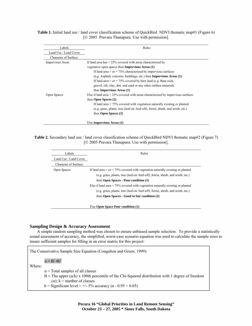

Over 500 sample points were generated for each thematic map using the ISODATA algorithm to insure good distribution across the study area Figure 6 and 7 show the accuracy assessment sites acquired for the entire classification of each QB NDVI thematic map To accomplish this ERDAS 87rsquos random number generator function was used to create random points from the QB NDVI thematic maps for comparison to the 2004 2 ft (06 m) and the 2002 05 ft (015 m) spatial resolution orthophotos The program automatically discarded random points not sufficiently representing relatively homogenous areas This function minimized registration errors of the image and helped to accurately interpret a true representation of each reference point on the orthophoto To assure visual interpretation consistency these reference points were individually evaluated by one team member with many years of photo interpretation experience In some cases there were conflicts due to lsquoleanrsquo in the orthophoto or mixed pixels around the edges These points were re-evaluated using the 2004 orthophoto Quality control was performed on the data set by the principal author Finally the error matrixes were generated and the overall and individual Kappa coefficients were calculated (Table 3 and 4)
Figure 6 Classification result of NDVI QuickBird thematic map 1and 502 accuracy sites
Figure 7 Classification result of NDVI QuickBird thematic map 2 and the accuracy assessment sites
Pecora 16 ldquoGlobal Priorities in Land Remote Sensingrdquo October 23 ndash 27 2005 Sioux Falls South Dakota
Table 3 Accuracy assessment result of NDVI QuickBird thematic map1
Accuracy Assessment - Unsupervised Thematic Map1(100 spectral clusters) Map Class Name
ID
Labeling
Criteria
Areas (Acres)
Areas ()
Reference Totals
Classified Totals
Number Correct
Producers Accuracy ()
Users Accuracy ()
Kappa Statistics
11 Impervious areas 1-40 127098 4372 258 216 210 8140 9722 09429 Open spaces 41-100 163581 5628 244 286 238 9754 8322 06734 Overall Classification Accuracy = 8924 Overall Kappa Statistics = 07857
12 Impervious areas 1-45 139227 4790 258 241 229 8876 9502 08976 Open spaces 46-100 151453 5210 244 261 232 9508 8889 07838 Overall Classification Accuracy = 9183 Overall Kappa Statistics = 08368
13 Impervious areas 1-50 152654 5252 258 261 247 9574 9464 08896 Open spaces 51-100 138025 4748 244 241 230 9426 9544 09112 Overall Classification Accuracy = 9502 Overall Kappa Statistics = 09003
14 Impervious areas 1-55 167757 5771 258 285 250 9690 8772 07473 Open spaces 56-100 122922 4229 244 217 209 8566 9631 09283 Overall Classification Accuracy = 9143 Overall Kappa Statistics = 0828
15 Impervious areas 1-60 184209 6337 258 306 251 9729 8203 06302 Open spaces 61-100 106470 3663 244 196 189 7746 9643 09305 Overall Classification Accuracy = 8765 Overall Kappa Statistics = 07515
Labeling spectral clusters the lower the numbers the darker the areas are label to impervious areas (low NDVI value) Labeling spectral clusters the higher the numbers are the brighter the areas are label to open spaces (high NDVI value)
Table 4 Accuracy assessment result of NDVI QuickBird thematic map2
Accuracy Assessment - Unsupervised Thematic Map2 (50 spectral clusters) Map Class Name
ID Open Spaces
Labeling
Criteria
Areas (Acres)
Areas ()
Reference Totals
Classified Totals
Number Correct
Producers Accuracy ()
Users Accuracy ()
Kappa Statistics
21 Poor 1-25 73066 2514 242 239 164 6777 6862 04547 Good to Fair 26-50 64959 2235 328 331 253 7713 7644 0445 Overall Classification Accuracy = 7316 Overall Kappa Statistics = 04498
22 Poor 1-30 90677 3119 242 309 197 8140 6375 03701 Good to Fair 31-50 47349 1629 328 261 216 6585 8276 05939 Overall Classification Accuracy = 7246 Overall Kappa Statistics = 0456
Labeling spectral clusters the lower the numbers the darker the areas are label to open spaces-poor condition (low NDVI value) Labeling spectral clusters the higher the numbers the brighter the areas are label to open spaces-good to fair condition (high NDVI value) GIS Spatial Modeling
A spatial modeling or analysis is a set of analytical procedures applied with a GIS A spatial model is a set of clearly defined analytical procedures that run on a spatial database to derive new information describing a new spatial relationship It is structured as a set of rules including a combination of logical expressions mathematical procedures and criteria built using analytical tools in GIS which are applied for the purpose of simulating the process (ESRI staff 1995)
In GIS there are three categories of spatial modeling functions that can be applied to geographic data objects (1) geometric models such as calculating the Euclidean distance between objects generating buffers calculating areas and perimeters and so on (2) coincidence models such as polygon overlay and (3) adjacency models (pathfinding redistricting and allocation) All three model categories support operations on geographic data objects such as points lines polygon TINS and grids (ESRI staff 1995)
In this study the geometric and coincidence modeling functions in ArcView33 geoprocessing were designed in a sequence of steps to build a spatial modeling based on the composite runoff index spatial model The process of spatial
Pecora 16 ldquoGlobal Priorities in Land Remote Sensingrdquo October 23 ndash 27 2005 Sioux Falls South Dakota
modeling created a new data set (ArcView shapefile) of geographic features Each shapefile contained new polygons that described new spatial relationships of the data sets among surface characteristics of land use land cover and hydrologic soil groups including its CN
Next is an example of applying the composite runoff index spatial model to develop spatial modeling for the composite of CNrsquos calculation within the study area Finally the CN results were compared to the TR-55 NRCS (1986) publication (Figure 5) in order to validate the utility of QB NDVI imagery as shown in Table 8
The Composite of Runoff Indexrsquos Spatial Model for SCS CN and SCS adjusted CN (copy 2005 Pravara Thanapura Use with permission)
CNcomposite = [ of area covered (ji) x CN(j)] Where CNcomposite is the sum of the component CN within a parcel boundary (i) delineated by the land activity code of the City of Sioux Falls (Table 5) of area covered is a component (j) of the area (i) divided by the total area (i) Note that the component of the area is a subset of polygon features delineated by surface characteristics of land use land cover (GIS layer = ArcView shapefile) derived from two QB NDVI thematic maps using the ISODATA algorithm and hydrologic soil group as described previously (Figure 8) CN(j) is a runoff curve number (Table 6)of the component (polygon)[j] of the area (i) determined by the surface characteristics and its hydrologic soil groups
Table 5 The 2004 parcel ndash activity codes and a set of rules
Activity Code and Description SCS CN Cover Type1 Rule by Area 11 Single family Residential districts by average lot size - gt= 01 and lt= 0125 acre Residential 18 acre (0125 acres or 50585 sqm2) gt= 40468 and lt= 50585 sqm2
11 Single family Residential districts by average lot size - gt 0125 and lt= 025 acre Residential 14 acre (025 acres or 101171 sqm2) gt 50585 and lt= 101171 sqm2
11 Single family Residential districts by average lot size - gt 025 and lt= 03330 acre Residential 13 acre (03330 acres or 134759 sqm2) gt 101171 and lt= 134759 sqm2
11 Single family Residential districts by average lot size - gt 03330 and lt= 05 acre Residential 12 acre (05 acres or 202341 sqm2) gt 134759 and lt= 202341 sqm2
11 Single family Residential districts by average lot size - gt 05 and lt= 1 acre Residential 1 acre (404683 sqm2) gt 202341and lt= 404683 sqm2
11 Single family Residential districts by average lot size - gt 1 and lt= 2 acres Residential 2 acres (809365 sqm2) gt 404683 and lt= 809365 sqm2
31 Banks and Financial Institutions Urban Districts - Commercial and business gt= 05 acres or 202341 sqm2
33 Other offices Urban Districts - Commercial and business gt= 05 acres or 202341 sqm2
64 Warehousing Distribution Urban Districts - Industrial gt= 05 acres or 202341 sqm2
and Wholesale 1 The samples of activity codes are similar to the cover type of the urban land cover of the runoff curve number table in the TR-55 NRCS (1986) publication [Figure 5]
Pecora 16 ldquoGlobal Priorities in Land Remote Sensingrdquo October 23 ndash 27 2005 Sioux Falls South Dakota
Figure 8 The runoff index GIS data sets derived from the 2004 parcel layer by activity codes delineated by
NDVI QuickBird information and hydrologic soil groups
Table 6 Runoff curve numbers in Percentage for the CN calculation defined from the TR-55 NRCS (1986) Publication (Figure 5)
Land Use Land Cover Curve numbers for
hydrologic Soil Group
Character of Surface A2 B3 C4 D5
Impervious Areas 98 98 98 98 Open Spaces - Poor Condition 68 79 86 89 Open Spaces - Good to Fair Condition1 49 69 79 84
1 CN of fair condition is use for open spaces ndash good to fair condition 1 A The soil characteristics are deep sand deep loess and aggregated silts (McCuen 1982) 2 B The soil characteristics are shallow loess and sandy loam (McCuen 1982) 3 C The soil characteristics are clay loams shallow sandy loam soils low in organic content and soils usually high in clay (McCuen 1982) 4 B The soil characteristics are swell significantly when wet heavy plastic clays and certain saline soils (McCuen 1982)
Pecora 16 ldquoGlobal Priorities in Land Remote Sensingrdquo October 23 ndash 27 2005 Sioux Falls South Dakota
Table 8 The CN Results and SCS CN comparison
GIS Activity Code SCS CN Cover Type1 Rule Samples Total CNID and by Area Areas2 Result
Description (avg) B3 Sample Area4
1 11 Single family Residential districts by average lot size - gt= 01 and lt= 0125 acres 312 3555 acres 8688 85 9994Residential 18 acre gt= 40468 and lt= 50585 sqm2 14386463 sqm2
(0125 acres or 50585 sqm2) 123 2 11 Single family Residential districts by average lot size - gt 0125 and lt= 025 acres 3284 5766 acres 8430 75 9976
Residential 14 acre gt 50585 and lt= 101171 sqm2 23333993 sqm2
(025 acres 101171 sqm2) 1987 3 11 Single family Residential districts by average lot size - gt 025 and lt= 03330 acres 357 10006 acres 8244 72 10000
Residential 13 acre gt 101171 and lt= 134759 sqm2 40492530 sqm2
(03330 acres 134759 sqm2) 345 4 11 Single family Residential districts by average lot size - gt 03330 and lt= 05 acres 140 5451 acres 8203 70 10000
Residential 12 acre gt 134759 and lt= 202341 sqm2 22059243 sqm2
(05 acres 202341 sqm2) 188 5 11 Single family Residential districts by average lot size - gt 05 and lt= 1 acres 43 261 acres 7684 68 9557
Residential 1 acre (404683 sqm2) gt 202341and lt= 404683 sqm2 10562213 sqm2
09 6 11 Single family Residential districts by average lot size - gt 1 and lt= 2 acres 4 456 acres 8527 65 10000
Residential 2 acres (809365 sqm2) gt 404683 and lt= 809365 sqm2 1845352 sqm2
016 7 31 Banks and Urban Districts - Commercial gt= 05 acres 17 1496 acres 9419 92 10000
Financial and business gt= 202341 sqm2 6054050 sqm2
Institutions 052 8 33 Other offices Urban Districts - Commercial gt= 05 acres 56 6396 acres 9321 92 10000
and business gt= 202341 sqm2 25883493 sqm2
22 9 64 Warehousing Urban Districts - Industrial gt= 05 acres 11 2004 acres 8631 88 9400
Distribution and gt= 202341 sqm2 8109837 sqm2
Wholesale 07 4224 89634 acres 8572 79 9881
362733112 sqm2
3089
SCS CNHydrologic Soil Group
Total
1 The samples of activity codes are similar to the cover type of the urban land cover of the runoff curve number table in the TR-55 NRCS (1986) publication [Figure 5] 2 The study area is 290142 acres (11742 hectares) 3The total area of hydrologic soil group B of each sample layer by parcel - activity code 4 B The soil characteristics are shallow loess and sandy loam (McCuen 1982)
RESULTS amp DISCUSSION
The overall accuracy of the two QB NDVI thematic maps produced is presented in Table 3 and Table 4 using classification schemes from Table 1 and Table 2 respectively Figure 6 and 7 shows the two NDVI QuickBird thematic maps with the highest overall classification accuracy used as a GIS input into the Sioux Falls spatial modeling for the composite of CNs calculations
Table 3 shows the overall accuracy results of mapping impervious areas and open spaces obtained from five different labeling criteria when the same unsupervised image of 100 spectral clusters was used The Map ID13 with the combination labeling criteria of impervious areas (DNs range between 1-50) and open spaces (DNs range between 51-100) achieved the highest overall Kappa value of 09003 with the overall classification accuracy of 9505 Comparing the accuracy results to the accuracy results obtained from other labeling criteria showed slightly differing classification accuracy improvement increasing toward the mid DNs of QB NDVI This pattern of change in classification accuracy showed the potential correlations between increasing and decreasing of the DNs and amounts of open spaces (vegetative areas) and impervious areas (non vegetative areas) [Figure 4] The DNs range from 126 to 0 indicates increasing impervious surfaces shown in shades of dark tones The DNs range from 126 to 255 indicates increasing openspaces shown in shades of light tones
Pecora 16 ldquoGlobal Priorities in Land Remote Sensingrdquo October 23 ndash 27 2005 Sioux Falls South Dakota
Table 4 shows the overall accuracy results of mapping two classes obtained from two different labeling criteria utilizing the same unsupervised image of 50 spectral clusters The overall Kappa value for the Map ID 21 and Map ID22 produced was only 044 and 045 respectively The results showed that the spectral classifications were not spectrally distinct among open spaces-poor and good-to-fair conditions Map ID21 was used in this study since its producer and user accuracy in percentages were similar which indicated higher map accuracy compare to Map ID22
Comparing the overall accuracy of the two thematic maps demonstrated using the labeling pixel criteria with the DNs 5050 spectral cluster thresholds for assigning labels into two classes was the best method to use This tended to improve classification accuracy with high Kappa values and similar percentages of producer and user accuracy
Finally the average CN values of different land use land cover descriptions covering homogeneous soil types were calculated and compared to the SCS CN The results of this comparison are shown in Table 8 in order to validate the utility of QB NDVI imagery for CN calculation The overall average CN covering approximately 30 of the study area produced was 85 and the average SCS CN was 79 Comparing CN value within GIS ID produced from different approaches demonstrated that the new design technological methodologies produced conservative CN results similar to those found in the SCS CN table
The finer resolution imagery used in this study allows for better discrimination in land use land cover and the accuracy results validate the hypothesis of this study This is reflected in the fact that overall accuracy for the two QB NDVI thematic maps produced was 95 and 73 respectively Additionally the average CN values among the GIS ID samples described as single family showed that decreasing average lot size produced higher CN numbers or higher runoff This indicates increasing amounts of impervious areas and decreasing amounts of green vegetation as expected
CONCLUSIONS
This applied research demonstrated that the proposed spatial modeling utilizing the fine spatial resolution remotely sensed data and a GIS approach were successful in accurately automating and mapping land use land cover surface characteristics and determining the runoff curve number in the urban hydrology for small watersheds Therefore the hypothesis of this study was accepted Mapping fine spatial resolution QuickBird NDVI imagery generated using the traditional unsupervised classification was a more accurate simpler and efficient data extraction approach that increased speed and potentially reduces costs of both the analysis and mapping process The application of this approach could be beneficial to municipal engineers involved with designing or maintaining stormwater management systems and drainage improvement projects
ACKNOWLEDGEMENTS
The author would like to thank the following employees of the City of Sioux Falls South Dakota for their contribution to the success of this research project Steve Van Aartsen GIS supervisor and his staff for all the data and information contributed for this project Jeff Dunn City Drainage Engineer for his time and the literature provided on hydrology in Sioux Falls and Sam Trebilcock Transportation Planner for his assistance and interest
The author would also like to thank the co authors for their support input effort and specialized expertise in making this project a success Additional thanks go to Mr Kevin Dalsted Director Engineering Resource Center South Dakota State University Brookings South Dakota for the use of the hardware and software that made this research possible
Pecora 16 ldquoGlobal Priorities in Land Remote Sensingrdquo October 23 ndash 27 2005 Sioux Falls South Dakota
REFERENCES
Bondelid TR TJ Jackson and RH McCuen 1982 Estimating runoff curve numbers using remote sensing data Singh Vijay P editor Applied modeling in catchment hydrology Water Resources Publications Littleton Colorado 563 p
Congalton R and K Green 1999 Assessing the Accuracy of Remotely Sensed Data Principles and Practices CRCLewis Press Boca Raton Florida 137 p
Chen DM and D Stow 2003 Strategies for integrating information from multiple spatial resolutions into land-use land-cover classification routines Photogrammetric Engineering amp Remote Sensing 69(11)1279-1287
Draper S E and S G Rao 1986 Runoff prediction using remote sensing imagery Water Resources Bulletin 22(6) 941-949 p
Dubayah R O E F Wood E T Engman K P Czajkowski M Zion and Rhoads 2000 Remote Sensing in Hydrology and Water Management Remote Sensing in Hydrology and Water Management Schultz G A and ET Engman editors Springer Germany 483 p
Engman E T 1982 Remote sensing applications in watershed modeling Applied modeling in catchment hydrology Singh Vijay P editor Water Resources Publications Littleton Colorado 563 p
Engman E T 1993 Remote Sensing Handbook of Hydrology Maidment David R editor New York McGraw- Hill 241-2423 p
Environmental Systems Research Institute Staff 1995 Understanding GIS Version 7 for UNIX and Open VMS John Wiley ampSons New York NY 500 p
Golding B L 1997 Discussion Runoff Curve Number Has It Reached Maturity Journal of Hydrologic Engineering 2(3) 145-148 p
Jackson T J and R M Ragan 1977 State-of-the-art application of Landsat data in urban hydrology International symposium on urban hydrology hydraulics and sediment control University of Kentucky Lexington Kentucky 275-285 p
McCuen R H 1982 A guide to hydrologic analysis using SCS methods NJ Prentice-Hall Englewood Cliffs NJ 145 p
McCuen R H 2002 Approach to confidence interval estimation for curve numbers Journal of Hydrologic Engineering 7(1) 43-48 p
McCuen R H 2003 Discussion of Approach to Confidence Interval Estimation for Curve Numbers Journal of Hydrologic Engineering 8(4) 232-233 p
McCuen R H and O Okunola 2002 Extension of TR-55 for Microwatersheds Journal of Hydrologic Engineering 7(4) 319-325 p
Melesse A M and W D Graham 2004 Storm runoff prediction based on a spatially distributed travel time method utilizing remote sensing and GIS Journal of the American Water Resources Association (JAWRA) 40(4) 863-879 p
Mishra S K and V P Singh 2003 Soil Conservation Service Curve Number (SCS-CN) methodology The Netherlands Kluwer Academic Publishers PO Box 17 3300 AA Dordrecht 536 p
Natural Resources Conservation Service (NRCS) 1972 SCS National Engineering Handbook Section 4 Hydrology URL httpwwwinfousdagovCEDftpCEDneh630-ch10pdf US Department of Agriculture Natural Resources Conservation Service (last date accessed 21 August 2005)
Natural Resources Conservation Service (NRCS) 1986 Urban hydrology for small watersheds TR-55 Technical release 55 URL httpwwwwccnrcsusdagovhydrohydro-tools-models-tr55html US Department of Agriculture National Water and Climate Water (last date accessed 21 August 2005)
Natural Resources Conservation Service (NRCS) 1992 Computer program for project formulation-hydrology Tech Release No 20 URL httpwwwwccnrcsusdagovhydrohydro-tools-models-tr20html US Department of Agriculture National Water and Climate Water (last date accessed 21 August 2005)
Ponce V M and R H Hawkins 1996 Runoff curve number has it reached maturity Journal of Hydrologic Engineering 1(1) 11-19p
Ragan R M and T J Jackson 1980 Runoff synthesis using Landsat and SCS model Journal of Hydraulics division Proceedings of the American Society of Civil Engineers (ASCE) 106(5) 667-678p
Schultz G A 1988 Remote sensing in Hydrology Journal of Hydrology 100(1-3) 239-265 p
Pecora 16 ldquoGlobal Priorities in Land Remote Sensingrdquo October 23 ndash 27 2005 Sioux Falls South Dakota
Schultz G A 1996 Remote sensing applications to hydrology Runoff Hydrological Sciences Journal 41(4) 453-475 p
Thomas J J and R H McCuen 1979 Accuracy of impervious area values estimated using remotely sensed data Water Resources Bulletin 27(3) 373-379 p
Pecora 16 ldquoGlobal Priorities in Land Remote Sensingrdquo October 23 ndash 27 2005 Sioux Falls South Dakota
- ABSTRACT
- METHODS
- Study Area
- Digital Data amp Pre-Processing
- Classification Approach
-
- REFERENCES
-
Mapping Urban Land Use Land Cover Using QuickBird NDVI Imagery for Runoff Curve Number Determination
Pravara Thanapura Engineering Resource Center
Suzette Burckhard Civil and Environmental Engineering
Mary Orsquo Neill Engineering Resource Center
Dwight Galster and Mathematics and Statistics
South Dakota State University Brookings
South Dakota 57007 USA
Eric Warmath
Department of Transportation State of Nevada
1263 S Stewart Street
Carson City Nevada 89712 USA
ABSTRACT
The objective of this study was to evaluate Normalized Difference Vegetation Index (NDVI) data derived from QuickBird (QB) satellite imagery to map impervious areas and open spaces for runoff curve number (CN) determination The image was collected on April 26 2004 and provided by the City of Sioux Falls SD The image was radiometrically and geometrically corrected prior to this study The imagery has four bands (including the blue green red and near-infrared) and was imaged at a 239-meter spatial resolution The red channel (band 3 630-690 nm) and the near infrared channel (band 4 760-900 nm) were used to create the QB NDVI dataset (Band 4 - Band3 Band 4 + Band3) This research employed the urban land cover classification scheme of the runoff curve number table in the TR-55 (NRCS 1986) publication An unsupervised spectral classification approach was used in this study The research hypothesis was that high-resolution NDVI could improve the efficiency and effectiveness of urban land cover data extraction For the accuracy assessment process a simple random sampling scheme was employed using a random number generator to select points from the classified QB NDVI imagery for comparison to the 06-meter spatial resolution orthoimage acquired on April 23 2004 The overall and individual Kappa coefficients were calculated The overall accuracy for the two QB NDVI thematic maps produced was 95 and 73 respectively The average CN values of homogeneous land use land cover and soil type covering approximately 30 of the study area were determined and compared to the SCS CN in order to validate the utility of QB NDVI imagery for CN calculation The overall average CN produced from the spatial modeling was 85 and the average SCS CN was 79
INTRODUCTION
Remote satellite sensing application in hydrology did not start until the first launch of Earth Resources Technology Satellite (ERTS) [later renamed Landsat 1] in July of 1970 QUOTE (Schultz 1988) (Schultz 1988) Remotely sensed data is rapidly becoming an important source of information in hydrologic modeling monitoring and research QUOTE (Engman 1982 Engman 1993 Melesse and Graham 2004) (Engman 1982 1993 Melesse and Graham 2004) QUOTE ADDIN PROCITE yuml1105lsquo190200000000010000)030000F5C_Procite5CPravara_Thanapura1pdt10Engman 1982 8100102000600agraveagrave000000iquestH00agrave1400yumlyumlyumlyuml00000000010000001400000001000000000000000A000000000000ordmI_˜lsaquoEuml00010000000100000000000000tograve12000notW00yumlyumlyumlyuml QUOTE ADDIN PROCITE yuml1105lsquo190200000000010000F030000F5C_Procite5CPravara_Thanapura1pdt1AMelesse amp Graham 2004 8450104000700agraveagrave000000iquestH00 7140014000000010000000000000000000000100000000000000003000000000000AtildeAcircw00000000yumlyumlyumlyuml07AumlAcircwTHORNAcircAcircw0000200uumlntilde1200atildeAcircAcircw0600agraveagrave000000iquestH00 714001400000001000000000000000000000010000000000000000A000000000000ordmI_hUgraveEuml00030000000500000000000000tograve12000notW00yumlyumlyumlyuml Its advantages include spectral radiometric spatial and temporal resolutions including its ability to generate information and to provide a means of observing hydrological state variables over large areas or small complex basins It offers an alternative to conventional data collection employed in the estimation of certain hydrologic model parameters The primary benefits obtainable from using remote sensing are the reduction of manpower time and monetary resources required for data collecting and processing For some situations remote sensing provides information that was previously impossible or impractical to obtain using conventional techniques QUOTE (Thomas and McCuen 1979) (Thomas and McCuen 1979) Therefore remote sensing technology is a very important tool for successful hydrologic model analysis prediction and validation The National Resource Conservation Service (NRCS) formally the Soil Conservation Service (SCS) has developed a series of hydrologic models in water resource planning and design The SCS Curve Number (SCS-CN) method is the best-known component of the SCS hydrologic models According to Ponce and Hawkins (1996) the origins of the CN methodology can be traced back to the thousand of infiltrometer tests carried out by SCS in the late 1930s and early 1940s The intent was to develop basic data to evaluate the effects of watershed treatment and soil conservation measures on the rainfall-runoff process A major catalyst for the development and implementation of the runoff CN methodology was the passage of the Watershed Protection and Flood Prevention Act (Public Law 83-566) in August 1954 The method and its use are described in the SCS National Engineering Handbook Section 4 Hydrology (NEH-4) QUOTE (Soil Conservation Service (SCS) 1972) [NRCS 1972] The document has since been revised in 1956 64 65 71 72 85 and 1993 The CN method is well established in hydrologic engineering and environmental impact analyses Its major advantage are (1) its simplicity (2) its predictability (3) its stability (4) its reliance on only one parameter and (5) its responsiveness to major runoff-producing watershed properties (soil type land covertreatment surface condition and antecedent condition) [ QUOTE (Ponce and Hawkins 1996) Ponce and Hawkins 1996] Consequently the methodology has been widely used in numerous applications by practicing engineers and hydrologists nationally and internationally QUOTE (McCuen 1982 Ponce and Hawkins 1996 Golding 1997 McCuen 2002 McCuen and Okunola 2002 Mishra and Singh 2003 McCuen 2003) (McCuen 1982 2002 2003 Ponce and Hawkins 1996 Golding 1997 McCuen and Okunola 2002 Mishra and Singh 2003) QUOTE ADDIN PROCITE yuml1105lsquo19020000000001000012030000F5C_Procite5CPravara_Thanapura1pdt11Golding 1997 7870102000700agraveagrave0C0000iquestH00xB1400yumlyumlyumlyuml00000000010000001400000001000000000000000A000000000000ordmI_Agrave08Ccedil00030000000500000000000000umlograve12000notW00yumlyumlyumlyuml QUOTE ADDIN PROCITE yuml1105lsquo19020000000001000013030000F5C_Procite5CPravara_Thanapura1pdt19Ponce amp Hawkins 1996 7880104000500agraveagrave000000iquestH00agrave1400yumlyumlyumlyuml000000000100000014000000010000000000000003000000000000002000000000019notAcircw00000000yumlyumlyumlyumlFnotAcircw000000003laquoAcircw0700agraveagrave000000iquestH00agrave1400yumlyumlyumlyuml00000000010000001400000001000000000000000A000000000000ordmI_deg0BIacute00030000000500000000000000umlograve12000notW00yumlyumlyumlyuml QUOTE ADDIN PROCITE yuml1105lsquo19020000000001000015030000F5C_Procite5CPravara_Thanapura1pdt10McCuen 2003 7900102000600agraveagrave000000iquestH00xB1400yumlyumlyumlyuml00000000010000001400000001000000000000000A000000000000ordmI_deg0BIacute00050000000500000000000000umlograve12000notW00yumlyumlyumlyuml QUOTE ADDIN PROCITE yuml1105lsquo1902000000000100001E030000F5C_Procite5CPravara_Thanapura1pdt1AMcCuen amp Okunola 2002 7990104000600agraveagrave000000iquestH00xB1400yumlyumlyumlyuml000000000100000014000000010000000000000003000000000000002000000000019notAcircw00000000yumlyumlyumlyumlFnotAcircw000000003laquoAcircw0700agraveagrave000000iquestH00xB1400yumlyumlyumlyuml00000000010000001400000001000000000000000A000000000000ordmI_deg0BIacute00050000000500000000000000umlograve12000notW00yumlyumlyumlyuml QUOTE ADDIN PROCITE yuml1105lsquo190200000000010000$030000F5C_Procite5CPravara_Thanapura1pdt10McCuen 1982 8050102000600agraveagrave000000iquestH00agrave1400yumlyumlyumlyuml00000000010000001400000001000000000000000A000000000000ordmI_08Ecirc00010000000100000000000000umlograve12000notW00yumlyumlyumlyuml QUOTE ADDIN PROCITE yuml1105lsquo1902000000000100006030000F5C_Procite5CPravara_Thanapura1pdt18Mishra amp Singh 2003 8230104000600agraveagrave000000iquestH00agrave1400yumlyumlyumlyuml000000000100000014000000010000000000000003000000000000002000000000019notAcircw00000000yumlyumlyumlyumlFnotAcircw000000003laquoAcircw0500agraveagrave000000iquestH00agrave1400yumlyumlyumlyuml00000000010000001400000001000000000000000A000000000000ordmI_08Ecirc00010000000100000000000000umlograve12000notW00yumlyumlyumlyuml
The CN is an index that represents the combined hydrologic effect of soil group land cover type agricultural land treatment class hydrologic condition and antecedent soil moisture QUOTE (McCuen 1982) (McCuen 1982) It is the best-known component of a series of SCS hydrologic models most noticeably the TR-55 QUOTE (Natural Resources Conservation Service (NRCS) 1986) (NRCS 1986) QUOTE Natural Resources Conservation Service United States Department of Agriculture 1986 822 procedures and the TR-20 computer model QUOTE (Natural Resources Conservation Service (NRCS) 1984 McCuen 2002) (NRCS 1992 McCuen 2002) QUOTE ADDIN PROCITE yuml1105lsquo19020000000001000011030000F5C_Procite5CPravara_Thanapura1pdt10McCuen 2002 7860102000600agraveagrave000000iquestH00agrave1400yumlyumlyumlyuml00000000010000001400000001000000000000000A000000000000ordmI_pograveEacute00050000000500000000000000umlograve12000notW00yumlyumlyumlyuml The CN calculation requires use of storm rainfall and associated streamflow data for annual floods to derive the best means of establishing run off curve numbers A CN of 100 represents a condition of zero potential retention or 100 runoff of incident precipitation
Determination of the CN has been traditionally a time-consuming and labor-intensive procedure A basic problem exists in quantifying detailed spatial extent and distribution of various land cover classes Therefore remote sensing technology has become one of the primary methods for acquiring land cover data for providing detailed mapping information as input into the CN method (Jackson and Ragan 1977 Engman 1982 1993 Draper and Rao 1986 Schultz 1996 Dubavah et al 2000)
In previous studies one of the main problems of using remotely sensed data for estimation of land cover is a spatial resolution issue Moderate spatial resolutions are insufficient to generate the detail necessary to utilize the published SCS land cover table used in the SCS procedures Egrave008000000010000000000200atilde120080000000500agraveagrave00000005lsquo|yumlyumlyumlyumlm05lsquo|THORNAcircAcircw0000010007000000`00000080000000500000000000005lsquo|yumlyumlyumlyumlm05lsquo|THORNAcircAcircw0000010007000000`00000080000000700agraveagrave00000005lsquo|yumlyumlyumlyumlm05lsquo|THORNAcircAcircw0000010007000000`000000800000007000000000000AtildeAcircw000020000000000IcircAtildeAcircw00000000yumlyumlyumlyuml07AumlAcircw0000000600agraveagrave00000005lsquo|0000200m05lsquo|THORNAcircAcircw0000010007000000latilde1200800010007000000000000AtildeAcircw000020000000000IcircAtildeAcircw00000000yumlyumlyumlyuml07AumlAcircw80000000600agraveagrave00000005lsquo|0000200m05lsquo|THORNAcircAcircw0000010007000000latilde1200800010006000000000000AtildeAcircw000020000000000IcircAtildeAcircw00000000yumlyumlyumlyuml07AumlAcircw8000000020000F5C_Procite5CPravara_Thanapura1pdt19Ragan amp Jackson 1980 6420104000500agraveagrave000000iquestH00agrave1400yumlyumlyumlyuml000000000100000014000000010000000000000003000000000000002000000000019notAcircw00000000yumlyumlyumlyumlFnotAcircw000000003laquoAcircw0700agraveagrave000000iquestH00agrave1400yumlyumlyumlyuml00000000010000001400000001000000000000000A000000000000ordmI_08Ecirc00010000000100000000000000umlograve12000notW00yumlyumlyumlyuml QUOTE (Ragan and Jackson 1980 Engman 1982 Engman 1993) (Ragan and Jackson 1980 Engman 1982 1993) QUOTE ADDIN PROCITE yuml1105lsquo190200000000010000 030000F5C_Procite5CPravara_Thanapura1pdt10Engman 1993 8010102000600agraveagrave000000iquestH00agrave1400yumlyumlyumlyuml00000000010000001400000001000000000000000A000000000000ordmI_08Ecirc00010000000100000000000000umlograve12000notW00yumlyumlyumlyuml QUOTE ADDIN PROCITE yuml1105lsquo190200000000010000)030000F5C_Procite5CPravara_Thanapura1pdt10Engman 1982 8100102000600agraveagrave000000iquestH00agrave1400yumlyumlyumlyuml00000000010000001400000001000000000000000A000000000000ordmI_08Ecirc00010000000100000000000000umlograve12000notW00yumlyumlyumlyuml Engman in 1982 and 1993 suggested that one must develop a land cover table analogous that is compatible to the Landsat data Landsat may not be acceptable in small areas with certain land cover types Bondelid et al (1982) stated that special care should be exercised in analyzing small watersheds that contain heterogeneous land cover causing the largest CN errors Engineering designs utilizing the curve number are widely used but the curve number is sensitive to errors in the estimated input values used to derive it QUOTE (Bondelid et al 1982) (Bondelid et al 1982 McCuen 2002)
Remote sensing GIS GPS and image processing technological capability have improved significantly since the previous studies Commercial high-resolution satellite imagery creates unique opportunities to address and potentially solve old problems The purpose of this applied research is to bridge remote sensing and GIS to produce scientific knowledge by designing technological methodologies for determining the composite of curve numbers in the urban hydrology for small watersheds technical release 55 (TR-55) table NRCS (1986) publication for practicing professionals in urban water resource planning The theoretical foundation is that mapping a high resolution NDVI image generated using the ISODATA algorithm is an efficient and effective information extraction approach for the composite of runoff curve number calculation
METHODS
In this research newly designed technological methodologies were proposed for mapping urban land use land cover using QuickBird NDVI imagery and developing GIS spatial modeling for generating the composite of curve numbers in the TR-55 table NRCS (1986) publication To achieve this goal a sequence for digital processing and analysis was proposed and implemented (Figure 1) In order to assess the utility of QB NDVI imagery and to validate the composite runoff curve number calculation using designed GIS spatial modeling various procedures and comparisons of the generated runoff coefficients were presented reviewed and validated by practicing professionals including the City Drainage Engineer and the City Geographic Information Systems manager for the City of Sioux Falls South Dakota in August 2005
Figure 1 Sequence for digital processing and analysis
Study Area
The City of Sioux Falls is located in southeastern South Dakota Sioux Falls covers 40208 acres (162716 hectares) and has a population of approximately 138000 Climatologically Sioux Falls is in a continental climate with an average rainfall of 2386 inches (606 cm) and approximately 40 inches (1016 cm) of snow annually The majority of the precipitation comes in spring and summer with May and June being the months of maximum precipitation for the region The study area for this project is centered on 43O 31rsquo 18rdquo north latitude and 96O 44rsquo 42rsquorsquo west longitude in the southwestern part of the city This area encompasses 290142 acres (11742 hectares) with various land use land cover types and includes all or part of 26 hydrological urban sub-basins (Figure 2)
(a) (b)
Figure 2 The 2004 images of the study area at the same scale(a) The QuickBird multi image (4-3-2) on the left and (b) The QuickBird NDVI image on the right
Digital Data amp Pre-Processing
The 2004 remotely sensed data and vector GIS data layers were provided by the City of Sioux Falls They include orthophoto mosaics with 2 ft (06 m) and 05 ft (015 m) resolution a QuickBird satellite image with 796 ft (239 m) resolution and include data layers such as parcels city limit boundary hydrography and streets The data sets were processed and merged to combine the remotely sensed data with the GIS layers for the study area The April 23 2004 orthophoto was used as a reference to integrate all data sets into the same map projection and unit with the Universal Transverse Mercator (UTM) map projection World Geodetic System (WGS) 1984 and horizontal units in feet Software used in this project consisted of ERDAS Imagine 87 ArcMap 9 ArcView 33 and Microsoft Excel 2002
The two digital orthophotographs were acquired on April 23 2004 and May 20 2002 respectively Both orthophotos were collected and scanned to meet the combined requirements of National Map Accuracy Standards 90 of all contours will be within frac12 contour interval and 90 of horizontal positions shall be within 130 of one inch at the specified map scale The specified horizontal map scale was 1 inch = 200 ft (609m) The flight height above terrain was 4000 ft (12192m) for a photo negative scale of 1 inch = 667 ft (2033m) Contour interval for the elevation data was 2 ft (061m) The radiometric density of the digital orthophotograph was 10 bits per channel with a geometric precision of 1 micron Both orthophotos were provided in UTM projection WGS84 datum and planar distance survey units in feet Additionally both orthophotos were subset to the study area and the 2002 orthophoto was degraded 3x3 using ERDAS Imagine 87 Overlaying of the subset orthophotos demonstrated good alignment between images Therefore an image to image registration was not required
The QuickBird leaf-on image was collected on April 26 2004 The image was radiometrically corrected and orthorectified prior to this study with UTM projection WGS84 datum and units in meters The imagery has four bands (including the blue green red and near-infrared) and was imaged at a 239-meter spatial resolution in unsigned 16 bit data type The subset QB image was created in unsigned 8 bit data type The image was observed with no signs of atmospheric contamination The statistical spectral information showed a normal distribution with similar mean median and mode values Geometric correction was performed The subset scene was registered to the 2004 orthophoto with 31 ground control points and the RMS was 06940 pixel Figure 3 demonstrates the result The red channel (band 3 630-690 nm) and the near infrared channel (band 4 760-900 nm) were processed to create the QB NDVI image (NDVI = Band 4 - Band3 Band 4 + Band3) in unsigned 8 bit data type for the study area
The 2004 NRCS SSURGO 124000 data set of the soil survey area (SSA) named ldquoMinnehaha County South Dakotardquo and its standard metadata files were downloaded from the Soil Data Mart at on June 7 2004 It is a digital soil survey and generally is the most detailed level of soil geographic data developed by the National Cooperative Soil Survey The soil layer was in a single zip file in ArcView shapefile format with a geographic coordinate system and using North American Datum (NAD) 1983 This layer was processed using ArcView 33 geoprocessing and Microsoft Excel 2002 to create a soil layer associated with hydrologic soil groups in the project coordinate system for this study area Overlaying of the soil hydro features to the subset QB image demonstrated a good fit Therefore a vector to image registration was not necessary
(a) (b)
Figure 3 The registered 2004 images comparison at same scale and location
(a) The QuickBird multi image (4-3-2) on the left with the 2004 Orthoimage (1-2-3) on the right
(b) The QuickBird NDVI image on the left with the 2004 Orthoimage (1-2-3) on the right
Classification Approach
With the recent development of new remote sensing systems there are an increasing number of commercially high resolution data available There is a considerable amount of previous research that has been devoted to exploring the magnitude and impact of spatial resolution on image analysis when changing scale from coarse to fine resolutions Due to the more heterogeneous spectral-radiometric characteristics within land use land cover unit portrayed in high resolution images many applications of traditional single-resolution classification approaches have not led to satisfactory results In general traditional single-resolution classification procedures such as supervised unsupervised and hybrid training approaches are inadequate for discriminating between land use land cover classes where spectralspatial features and spatial patterns vary as a function of spatial resolution Consequently there is an increasing need of researching for more efficient approaches to process and analyze these data products (Chen and Stow 2003)
In this research the relatively simple Normalized Difference Vegetation Index (NDVI) was introduced in order to reduce heterogeneous spectral-radiometric characteristics within land use land cover surfaces portrayed in high resolution images It also was used for improving the accuracy level of details for mapping impervious surfaces and open spaces with different hydrologic conditions as used in the proposed SCS runoff curve number (CN) calculation in this study Additionally this research presented applying the principle behind NDVI using high spatial resolution QuickBird imagery based on the unique interaction differences in land use land cover surfaces with reflected or emitted electromagnetic radiation between QB Red band (630-690nm) and QB NIR band (760-900nm)
NDVI has been shown to correlate green leaf biomass and green leaf area index Chlorophylls the primary photosynthetic pigments in green plants absorb light primarily from the red and blue portions of the spectrum while a higher proportion of infrared is reflected or scattered As a result vigorously growing healthy vegetation has low red-light reflectance and high near-infrared reflectance and hence high NDVI values Impervious surfaces (eg Asphalt concrete buildings etc) and bare land (eg bare soil rock dirt etc) have similar reflectance in the red and the near infrared so these surfaces will have values near zero NDVI is calculated using the formula (Near infrared ndash red)(Near infrared + red) This relatively simply algorithm produces output values in the range of -10 to 10
Figure 4 shows a visual comparison of spectral correlation between QuickBird NDVI in unsigned 8 bit data type (0-255) for impervious areas and open spaces in the urban environment The impervious surfaces are the dark areas with low NDVI DNs and the brighter areas are vegetative covers with high NDVI DNs
(a) The 2004 QuickBird NDVI (b) The QuickBird multi image (4-3-2)
(c) The 2004 Orthophoto (1-2-3)
Figure 4 The registered 2004 images visual comparison of impervious areas and vegetative open spaces at same scale and location in residential areas
This research employed the urban land cover of the runoff curve number table in the TR-55 NRCS (1986) publication (Figure 5) The classification schemes defined from the TR-55 are detailed in Table 1 and Table 2 The defined classification schemes were used to generate two QB NDVI thematic maps using the ISODATA algorithm Gaussian Maximum Likelihood Classifier with ERDAS Imagine 87 assigning unsupervised spectral classes and assessing the accuracy of the maps The detailed map information from the second thematic map was then converted as a GIS input into a spatial modeling for calculating the composite of CNrsquos using the composite runoff index spatial model below
This spatial model based on the composite of the CNrsquos equation below can be applied for calculating the runoff index for both the SCS CN method and the rational method the CN number calculated for the SCS CN method and a runoff coefficient is the ldquocrdquo value used in the rational method recommended by the American Society of Civil Engineers and the Water Pollution Control Federation
The Composite of Runoff Indexrsquos Spatial Model (copy 2005 Pravara Thanapura Use with permission)
Runoff Indexcomposite = ( [ of area covered (ji) x CN(j)]
Where
CNcomposite is the sum of the component runoff index within an area (i) delineated by description of area
of area covered (ji) is the component (j) of the area (i) divided by the total area (i) Note that the component of the area is delineated by surface characteristics of land use land cover andor hydrologic soil group
CN(j) is a runoff index of the component (j) of the area (i) determined by the surface characteristics andor its hydrologic soil groups
The Composite CNrsquos Weigh Average Equation
CNcomposite = ( [ of area covered x CN] Where CNcomposite is the sum of composite runoff curve number within an area
of area covered is a component of the area divided by the total area
CN is the runoff curve number of the area
In this study the composite of CNrsquos calculation requires the combined surface characteristics and hydrologic effect of soil groups The surface characteristic was derived from the two QB NDVI thematic maps and the hydrologic soil groups were obtained from the 2004 NRCS SSURGO 124000 data set The soil information covered by hydrologic areas such as rivers or canals are not surveyed or were not available in this data set Therefore they were excluded from the decision rules Swimming pools were considered as impervious areas since these small size water features appeared spectrally impervious on the QB NDVI Additionally they retain precipitation and act as pervious surfaces during storms thus the decision rules would result in a conservative calculation of CNrsquos
There is one heavy industrial area in the southern part of the study area This area was an oil and fuel storage facility The tanks and their associated grass covered containment areas approximately 038 of the study areas 290142 acres (11742 hectares) The tank structures themselves were impervious but they were spectrally ruled as open spaces which resulted in a conservative composite CN calculation Precipitation falling on the containment areas does not interact with the surface and groundwater since precipitation falling in these areas evaporates naturally or is pumped out and treated as wastewater
Figure 5 TR-55 runoff curve number table for urban areas 14001400000001000000000000000000000010000000000000000A000000000000ordmI_cedil13Eacute00030000000500000000000000tograve12000notW00yumlyumlyumlyuml QUOTE (United States Department of Agriculture 1986) (United States Department of Agriculture 1986)
Table 1 Initial land use land cover classification scheme of QuickBird NDVI thematic map1 (Figure 6)[copy 2005 Pravara Thanapura Use with permission]
Table 2 Secondary land use land cover classification scheme of QuickBird NDVI thematic map2 (Figure 7)
[copy 2005 Pravara Thanapura Use with permission]
Sampling Design amp Accuracy Assessment
A simple random sampling method was chosen to ensure unbiased sample selection To provide a statistically sound assessment of accuracy the simplified worst-case scenario equation was used to calculate the sample sizes to insure sufficient samples for filling in an error matrix for this project
The Conservative Sample Size Equation (Congalton and Green 1999)
n = B 4b2
Where
n = Total samples of all classes
B = The upper (αk) x 100th percentile of the Chi-Squared distribution with 1 degree of freedom (α) k = number of classes
b = Significant level = +- 5 accuracy (α - 095 = 005)
Over 500 sample points were generated for each thematic map using the ISODATA algorithm to insure good distribution across the study area Figure 6 and 7 show the accuracy assessment sites acquired for the entire classification of each QB NDVI thematic map To accomplish this ERDAS 87rsquos random number generator function was used to create random points from the QB NDVI thematic maps for comparison to the 2004 2 ft (06 m) and the 2002 05 ft (015 m) spatial resolution orthophotos The program automatically discarded random points not sufficiently representing relatively homogenous areas This function minimized registration errors of the image and helped to accurately interpret a true representation of each reference point on the orthophoto To assure visual interpretation consistency these reference points were individually evaluated by one team member with many years of photo interpretation experience In some cases there were conflicts due to lsquoleanrsquo in the orthophoto or mixed pixels around the edges These points were re-evaluated using the 2004 orthophoto Quality control was performed on the data set by the principal author Finally the error matrixes were generated and the overall and individual Kappa coefficients were calculated (Table 3 and 4)
Figure 6 Classification result of NDVI QuickBird thematic map 1and 502 accuracy sites
Figure 7 Classification result of NDVI QuickBird thematic map 2 and the accuracy assessment sites
Table 3 Accuracy assessment result of NDVI QuickBird thematic map1
Labeling spectral clusters the lower the numbers the darker the areas are label to impervious areas (low NDVI value)
Labeling spectral clusters the higher the numbers are the brighter the areas are label to open spaces (high NDVI value)
Table 4 Accuracy assessment result of NDVI QuickBird thematic map2
Labeling spectral clusters the lower the numbers the darker the areas are label to open spaces-poor condition (low NDVI value)
Labeling spectral clusters the higher the numbers the brighter the areas are label to open spaces-good to fair condition (high NDVI value)
GIS Spatial Modeling
A spatial modeling or analysis is a set of analytical procedures applied with a GIS A spatial model is a set of clearly defined analytical procedures that run on a spatial database to derive new information describing a new spatial relationship It is structured as a set of rules including a combination of logical expressions mathematical procedures and criteria built using analytical tools in GIS which are applied for the purpose of simulating the process QUOTE (Environmental Systems Research Institude 1995) (ESRI staff 1995)
In GIS there are three categories of spatial modeling functions that can be applied to geographic data objects (1) geometric models such as calculating the Euclidean distance between objects generating buffers calculating areas and perimeters and so on (2) coincidence models such as polygon overlay and (3) adjacency models (pathfinding redistricting and allocation) All three model categories support operations on geographic data objects such as points lines polygon TINS and grids QUOTE (Environmental Systems Research Institude 1995) (ESRI staff 1995)
In this study the geometric and coincidence modeling functions in ArcView33 geoprocessing were designed in a sequence of steps to build a spatial modeling based on the composite runoff index spatial model The process of spatial modeling created a new data set (ArcView shapefile) of geographic features Each shapefile contained new polygons that described new spatial relationships of the data sets among surface characteristics of land use land cover and hydrologic soil groups including its CN
Next is an example of applying the composite runoff index spatial model to develop spatial modeling for the composite of CNrsquos calculation within the study area Finally the CN results were compared to the TR-55 NRCS (1986) publication (Figure 5) in order to validate the utility of QB NDVI imagery as shown in Table 8
The Composite of Runoff Indexrsquos Spatial Model for SCS CN and SCS adjusted CN (copy 2005 Pravara Thanapura Use with permission)
CNcomposite = ( [ of area covered (ji) x CN(j)]
WhereCNcomposite is the sum of the component CN within a parcel boundary (i) delineated by the land activity code of the City of Sioux Falls (Table 5)
of area covered is a component (j) of the area (i) divided by the total area (i) Note that the component of the area is a subset of polygon features delineated by surface characteristics of land use land cover (GIS layer = ArcView shapefile) derived from two QB NDVI thematic maps using the ISODATA algorithm and hydrologic soil group as described previously (Figure 8)
CN(j) is a runoff curve number (Table 6)of the component (polygon)[j] of the area (i) determined by the surface characteristics and its hydrologic soil groups
Table 5 The 2004 parcel ndash activity codes and a set of rules
1 The samples of activity codes are similar to the cover type of the urban land cover of the runoff curve number table in the TR-55 NRCS (1986) publication [Figure 5]
Figure 8 The runoff index GIS data sets derived from the 2004 parcel layer by activity codes delineated by NDVI QuickBird information and hydrologic soil groups
Table 6 Runoff curve numbers in Percentage for the CN calculation defined from the TR-55 NRCS (1986) Publication (Figure 5)
1 CN of fair condition is use for open spaces ndash good to fair condition1 A The soil characteristics are deep sand deep loess and aggregated silts (McCuen 1982)
2 B The soil characteristics are shallow loess and sandy loam (McCuen 1982)
3 C The soil characteristics are clay loams shallow sandy loam soils low in organic content and soils usually high in clay (McCuen 1982)
4 B The soil characteristics are swell significantly when wet heavy plastic clays and certain saline soils (McCuen 1982)
Table 8 The CN Results and SCS CN comparison
GISActivity Code SCS CN Cover Type1RuleSamplesTotal CN
IDand by AreaAreas2Result
Description (avg)
B
3
Sample Area
4
111 Single familyResidential districts by average lot size - gt= 01 and lt= 0125 acres3123555 acres8688859994
Residential 18 acre
gt= 40468 and lt= 50585 sqm
2
14386463 sqm
2
(0125 acres or 50585 sqm
2
)
123
211 Single familyResidential districts by average lot size - gt 0125 and lt= 025 acres32845766 acres8430759976
Residential 14 acre
gt 50585 and lt= 101171 sqm
2
23333993 sqm
2
(025 acres 101171 sqm
2
)
1987
311 Single familyResidential districts by average lot size - gt 025 and lt= 03330 acres35710006 acres82447210000
Residential 13 acre
gt 101171 and lt= 134759 sqm
2
40492530 sqm
2
(03330 acres 134759 sqm
2
)
345
411 Single familyResidential districts by average lot size - gt 03330 and lt= 05 acres1405451 acres82037010000
Residential 12 acre
gt 134759 and lt= 202341 sqm
2
22059243 sqm
2
(05 acres 202341 sqm
2
)
188
511 Single familyResidential districts by average lot size - gt 05 and lt= 1 acres43261 acres7684689557
Residential 1 acre (404683 sqm
2
)gt 202341and lt= 404683 sqm
2
10562213 sqm
2
09
611 Single familyResidential districts by average lot size - gt 1 and lt= 2 acres4456 acres85276510000
Residential 2 acres (809365 sqm
2
)gt 404683 and lt= 809365 sqm
2
1845352 sqm
2
016
731 Banks and Urban Districts - Commercial gt= 05 acres 171496 acres94199210000
Financial and business
gt= 202341 sqm
2
6054050 sqm
2
Institutions 052
833 Other officesUrban Districts - Commercialgt= 05 acres566396 acres93219210000
and business
gt= 202341 sqm
2
25883493 sqm
2
22
964 Warehousing Urban Districts - Industrialgt= 05 acres112004 acres8631889400
Distribution and
gt= 202341 sqm
2
8109837 sqm
2
Wholesale 07
422489634 acres8572799881
362733112 sqm
2
3089
SCS CN
Hydrologic Soil Group
Total
1 The samples of activity codes are similar to the cover type of the urban land cover of the runoff curve number table in the TR-55 NRCS (1986) publication [Figure 5]
2 The study area is 290142 acres (11742 hectares)
3The total area of hydrologic soil group B of each sample layer by parcel - activity code4 B The soil characteristics are shallow loess and sandy loam (McCuen 1982)
RESULTS amp DISCUSSION
The overall accuracy of the two QB NDVI thematic maps produced is presented in Table 3 and Table 4 using classification schemes from Table 1 and Table 2 respectively Figure 6 and 7 shows the two NDVI QuickBird thematic maps with the highest overall classification accuracy used as a GIS input into the Sioux Falls spatial modeling for the composite of CNs calculations
Table 3 shows the overall accuracy results of mapping impervious areas and open spaces obtained from five different labeling criteria when the same unsupervised image of 100 spectral clusters was used The Map ID13 with the combination labeling criteria of impervious areas (DNs range between 1-50) and open spaces (DNs range between 51-100) achieved the highest overall Kappa value of 09003 with the overall classification accuracy of 9505 Comparing the accuracy results to the accuracy results obtained from other labeling criteria showed slightly differing classification accuracy improvement increasing toward the mid DNs of QB NDVI This pattern of change in classification accuracy showed the potential correlations between increasing and decreasing of the DNs and amounts of open spaces (vegetative areas) and impervious areas (non vegetative areas) [Figure 4] The DNs range from 126 to 0 indicates increasing impervious surfaces shown in shades of dark tones The DNs range from 126 to 255 indicates increasing openspaces shown in shades of light tones
Table 4 shows the overall accuracy results of mapping two classes obtained from two different labeling criteria utilizing the same unsupervised image of 50 spectral clusters The overall Kappa value for the Map ID 21 and Map ID22 produced was only 044 and 045 respectively The results showed that the spectral classifications were not spectrally distinct among open spaces-poor and good-to-fair conditions Map ID21 was used in this study since its producer and user accuracy in percentages were similar which indicated higher map accuracy compare to Map ID22
Comparing the overall accuracy of the two thematic maps demonstrated using the labeling pixel criteria with the DNs 5050 spectral cluster thresholds for assigning labels into two classes was the best method to use This tended to improve classification accuracy with high Kappa values and similar percentages of producer and user accuracy
Finally the average CN values of different land use land cover descriptions covering homogeneous soil types were calculated and compared to the SCS CN The results of this comparison are shown in Table 8 in order to validate the utility of QB NDVI imagery for CN calculation The overall average CN covering approximately 30 of the study area produced was 85 and the average SCS CN was 79 Comparing CN value within GIS ID produced from different approaches demonstrated that the new design technological methodologies produced conservative CN results similar to those found in the SCS CN table
The finer resolution imagery used in this study allows for better discrimination in land use land cover and the accuracy results validate the hypothesis of this study This is reflected in the fact that overall accuracy for the two QB NDVI thematic maps produced was 95 and 73 respectively Additionally the average CN values among the GIS ID samples described as single family showed that decreasing average lot size produced higher CN numbers or higher runoff This indicates increasing amounts of impervious areas and decreasing amounts of green vegetation as expected
CONCLUSIONS
This applied research demonstrated that the proposed spatial modeling utilizing the fine spatial resolution remotely sensed data and a GIS approach were successful in accurately automating and mapping land use land cover surface characteristics and determining the runoff curve number in the urban hydrology for small watersheds Therefore the hypothesis of this study was accepted Mapping fine spatial resolution QuickBird NDVI imagery generated using the traditional unsupervised classification was a more accurate simpler and efficient data extraction approach that increased speed and potentially reduces costs of both the analysis and mapping process The application of this approach could be beneficial to municipal engineers involved with designing or maintaining stormwater management systems and drainage improvement projects
AcknowleDgements
The author would like to thank the following employees of the City of Sioux Falls South Dakota for their contribution to the success of this research project Steve Van Aartsen GIS supervisor and his staff for all the data and information contributed for this project Jeff Dunn City Drainage Engineer for his time and the literature provided on hydrology in Sioux Falls and Sam Trebilcock Transportation Planner for his assistance and interest
The author would also like to thank the co authors for their support input effort and specialized expertise in making this project a success Additional thanks go to Mr Kevin Dalsted Director Engineering Resource Center South Dakota State University Brookings South Dakota for the use of the hardware and software that made this research possible
References
Bondelid TR TJ Jackson and RH McCuen 1982 Estimating runoff curve numbers using remote sensing data Singh Vijay P editor Applied modeling in catchment hydrology Water Resources Publications Littleton Colorado 563 p
Congalton R and K Green 1999 Assessing the Accuracy of Remotely Sensed Data Principles and Practices CRCLewis Press Boca Raton Florida 137 p
Chen DM and D Stow 2003 Strategies for integrating information from multiple spatial resolutions into land-use land-cover classification routines Photogrammetric Engineering amp Remote Sensing 69(11)1279-1287
Draper S E and S G Rao 1986 Runoff prediction using remote sensing imagery Water Resources Bulletin 22(6) 941-949 p
Dubayah R O E F Wood E T Engman K P Czajkowski M Zion and Rhoads 2000 Remote Sensing in Hydrology and Water Management Remote Sensing in Hydrology and Water Management Schultz G A and ET Engman editors Springer Germany 483 p
Engman E T 1982 Remote sensing applications in watershed modeling Applied modeling in catchment hydrology Singh Vijay P editor Water Resources Publications Littleton Colorado 563 p
Engman E T 1993 Remote Sensing Handbook of Hydrology Maidment David R editor New York McGraw- Hill 241-2423 p
Environmental Systems Research Institute Staff 1995 Understanding GIS Version 7 for UNIX and Open VMS John Wiley ampSons New York NY 500 p
Golding B L 1997 Discussion Runoff Curve Number Has It Reached Maturity Journal of Hydrologic Engineering 2(3) 145-148 p
Jackson T J and R M Ragan 1977 State-of-the-art application of Landsat data in urban hydrology International symposium on urban hydrology hydraulics and sediment control University of Kentucky Lexington Kentucky 275-285 p
McCuen R H 1982 A guide to hydrologic analysis using SCS methods NJ Prentice-Hall Englewood Cliffs NJ 145 p
McCuen R H 2002 Approach to confidence interval estimation for curve numbers Journal of Hydrologic Engineering 7(1) 43-48 p
McCuen R H 2003 Discussion of Approach to Confidence Interval Estimation for Curve Numbers Journal of Hydrologic Engineering 8(4) 232-233 p
McCuen R H and O Okunola 2002 Extension of TR-55 for Microwatersheds Journal of Hydrologic Engineering 7(4) 319-325 p
Melesse A M and W D Graham 2004 Storm runoff prediction based on a spatially distributed travel time method utilizing remote sensing and GIS Journal of the American Water Resources Association (JAWRA) 40(4) 863-879 p
Mishra S K and V P Singh 2003 Soil Conservation Service Curve Number (SCS-CN) methodology The Netherlands Kluwer Academic Publishers PO Box 17 3300 AA Dordrecht 536 p
Natural Resources Conservation Service (NRCS) 1972 SCS National Engineering Handbook Section 4 Hydrology URL httpwwwinfousdagovCEDftpCEDneh630-ch10pdf US Department of Agriculture Natural Resources Conservation Service (last date accessed 21 August 2005)
Natural Resources Conservation Service (NRCS) 1986 Urban hydrology for small watersheds TR-55 Technical release 55 URL httpwwwwccnrcsusdagovhydrohydro-tools-models-tr55html US Department of Agriculture National Water and Climate Water (last date accessed 21 August 2005)
Natural Resources Conservation Service (NRCS) 1992 Computer program for project formulation-hydrology Tech Release No 20 URL httpwwwwccnrcsusdagovhydrohydro-tools-models-tr20html US Department of Agriculture National Water and Climate Water (last date accessed 21 August 2005)
Ponce V M and R H Hawkins 1996 Runoff curve number has it reached maturity Journal of Hydrologic Engineering 1(1) 11-19p
Ragan R M and T J Jackson 1980 Runoff synthesis using Landsat and SCS model Journal of Hydraulics division Proceedings of the American Society of Civil Engineers (ASCE) 106(5) 667-678p
Schultz G A 1988 Remote sensing in Hydrology Journal of Hydrology 100(1-3) 239-265 p
Schultz G A 1996 Remote sensing applications to hydrology Runoff Hydrological Sciences Journal 41(4) 453-475 p
Thomas J J and R H McCuen 1979 Accuracy of impervious area values estimated using remotely sensed data Water Resources Bulletin 27(3) 373-379 p
Digital Data13
darr13
Pre-Processing 13
Data Merging and Integration 13
darr13
Decision and Classification13
darr13
Image Classification13
Unsupervised ndash ISODATA Algorithm13
darr13
Classification Output13
darr13
Assess Accuracy13
darr13
Reports and GIS Data13
darr13
GIS Spatial Modeling13
The Composite of Runoff Curve Number Calculation13
darr13
Reject Accept Hypothesis13
13
13
Land Use Land Cover
Curve numbers for
hydrologic Soil Group
Character of Surface
A2
B3
C4
D5
Impervious Areas
98
98
98
98
Open Spaces - Poor Condition
68
79
86
89
Open Spaces - Good to Fair Condition1
49
69
79
84
Activity Code and Description
SCS CN Cover Type1
Rule by Area
11 Single family
Residential districts by average lot size -
gt= 01 and lt= 0125 acre
Residential 18 acre (0125 acres or 50585 sqm2)
gt= 40468 and lt= 50585 sqm2
11 Single family
Residential districts by average lot size -
gt 0125 and lt= 025 acre
Residential 14 acre (025 acres or 101171 sqm2)
gt 50585 and lt= 101171 sqm2
11 Single family
Residential districts by average lot size -
gt 025 and lt= 03330 acre
Residential 13 acre (03330 acres or 134759 sqm2)
gt 101171 and lt= 134759 sqm2
11 Single family
Residential districts by average lot size -
gt 03330 and lt= 05 acre
Residential 12 acre (05 acres or 202341 sqm2)
gt 134759 and lt= 202341 sqm2
11 Single family
Residential districts by average lot size -
gt 05 and lt= 1 acre
Residential 1 acre (404683 sqm2)
gt 202341and lt= 404683 sqm2
11 Single family
Residential districts by average lot size -
gt 1 and lt= 2 acres
Residential 2 acres (809365 sqm2)
gt 404683 and lt= 809365 sqm2
31 Banks and Financial Institutions
Urban Districts - Commercial and business
gt= 05 acres or 202341 sqm2
33 Other offices
Urban Districts - Commercial and business
gt= 05 acres or 202341 sqm2
64 Warehousing Distribution
Urban Districts - Industrial
gt= 05 acres or 202341 sqm2
and Wholesale
Accuracy Assessment - Unsupervised Thematic Map2 (50 spectral clusters)
Map
Class Name
Labeling Criteria
Areas (Acres)
Areas ()
Reference Totals
Classified Totals
Number Correct
Producers Accuracy ()
Users Accuracy ()
Kappa Statistics
ID
Open Spaces
21
Poor
1-25
73066
2514
242
239
164
6777
6862
04547
Good to Fair
26-50
64959
2235
328
331
253
7713
7644
0445
Overall Classification Accuracy = 7316
Overall Kappa Statistics = 04498
22
Poor
1-30
90677
3119
242
309
197
8140
6375
03701
Good to Fair
31-50
47349
1629
328
261
216
6585
8276
05939
Overall Classification Accuracy = 7246
Overall Kappa Statistics = 0456
Accuracy Assessment - Unsupervised Thematic Map1(100 spectral clusters)
Map
Class Name
Labeling Criteria
Areas (Acres)
Areas ()
Reference Totals
Classified Totals
Number Correct
Producers Accuracy ()
Users Accuracy ()
Kappa Statistics
ID
11
Impervious areas
1-40
127098
4372
258
216
210
8140
9722
09429
Open spaces
41-100
163581
5628
244
286
238
9754
8322
06734
Overall Classification Accuracy = 8924
Overall Kappa Statistics = 07857
12
Impervious areas
1-45
139227
4790
258
241
229
8876
9502
08976
Open spaces
46-100
151453
5210
244
261
232
9508
8889
07838
Overall Classification Accuracy = 9183
Overall Kappa Statistics = 08368
13
Impervious areas
1-50
152654
5252
258
261
247
9574
9464
08896
Open spaces
51-100
138025
4748
244
241
230
9426
9544
09112
Overall Classification Accuracy = 9502
Overall Kappa Statistics = 09003
14
Impervious areas
1-55
167757
5771
258
285
250
9690
8772
07473
Open spaces
56-100
122922
4229
244
217
209
8566
9631
09283
Overall Classification Accuracy = 9143
Overall Kappa Statistics = 0828
15
Impervious areas
1-60
184209
6337
258
306
251
9729
8203
06302
Open spaces
61-100
106470
3663
244
196
189
7746
9643
09305
Overall Classification Accuracy = 8765
Overall Kappa Statistics = 07515
Labels
Rules
Land Use Land Cover
Character of Surface
Open Spaces
If land area = or lt 75 covered with vegetation naturally existing or planted
(eg grass plants tree (leaf-on leaf-off) forest shrub and scrub etc)
then Open Spaces - Poor condition (1)
Else if land area gt 75 covered with vegetation naturally existing or planted
(eg grass plants tree (leaf-on leaf-off) forest shrub and scrub etc)
then Open Spaces - Good to fair condition (2)
Else Open Space Poor condition (1)
Labels
Rules
Land Use Land Cover
Character of Surface
Impervious Areas
If land area has lt 25 covered with areas characterized by
vegetative open spaces then Impervious Areas (1)
If land area gt or = 75 characterized by impervious surfaces
(eg Asphalt concrete buildings etc) then Impervious Areas (1)
If land area gt or = 75 covered by bare land (eg Bare rock
gravel silt clay dirt and sand or any other earthen materials
then Impervious Areas (1)
Open Spaces
Else if land area lt 25 covered with areas characterized by impervious surfaces
then Open Spaces (2)
If land area gt 75 covered with vegetation naturally existing or planted
(eg grass plants tree (leaf-on leaf-off) forest shrub and scrub etc)
then Open Spaces (2)
Else Impervious Areas (1)
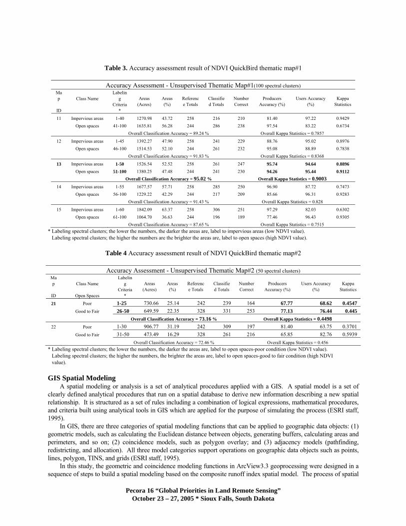
Table 3 Accuracy assessment result of NDVI QuickBird thematic map1
Accuracy Assessment - Unsupervised Thematic Map1(100 spectral clusters) Map Class Name
ID
Labeling
Criteria
Areas (Acres)
Areas ()
Reference Totals
Classified Totals
Number Correct
Producers Accuracy ()
Users Accuracy ()
Kappa Statistics
11 Impervious areas 1-40 127098 4372 258 216 210 8140 9722 09429 Open spaces 41-100 163581 5628 244 286 238 9754 8322 06734 Overall Classification Accuracy = 8924 Overall Kappa Statistics = 07857
12 Impervious areas 1-45 139227 4790 258 241 229 8876 9502 08976 Open spaces 46-100 151453 5210 244 261 232 9508 8889 07838 Overall Classification Accuracy = 9183 Overall Kappa Statistics = 08368
13 Impervious areas 1-50 152654 5252 258 261 247 9574 9464 08896 Open spaces 51-100 138025 4748 244 241 230 9426 9544 09112 Overall Classification Accuracy = 9502 Overall Kappa Statistics = 09003
14 Impervious areas 1-55 167757 5771 258 285 250 9690 8772 07473 Open spaces 56-100 122922 4229 244 217 209 8566 9631 09283 Overall Classification Accuracy = 9143 Overall Kappa Statistics = 0828
15 Impervious areas 1-60 184209 6337 258 306 251 9729 8203 06302 Open spaces 61-100 106470 3663 244 196 189 7746 9643 09305 Overall Classification Accuracy = 8765 Overall Kappa Statistics = 07515
Labeling spectral clusters the lower the numbers the darker the areas are label to impervious areas (low NDVI value) Labeling spectral clusters the higher the numbers are the brighter the areas are label to open spaces (high NDVI value)
Table 4 Accuracy assessment result of NDVI QuickBird thematic map2
Accuracy Assessment - Unsupervised Thematic Map2 (50 spectral clusters) Map Class Name
ID Open Spaces
Labeling
Criteria
Areas (Acres)
Areas ()
Reference Totals
Classified Totals
Number Correct
Producers Accuracy ()
Users Accuracy ()
Kappa Statistics
21 Poor 1-25 73066 2514 242 239 164 6777 6862 04547 Good to Fair 26-50 64959 2235 328 331 253 7713 7644 0445 Overall Classification Accuracy = 7316 Overall Kappa Statistics = 04498
22 Poor 1-30 90677 3119 242 309 197 8140 6375 03701 Good to Fair 31-50 47349 1629 328 261 216 6585 8276 05939 Overall Classification Accuracy = 7246 Overall Kappa Statistics = 0456
Labeling spectral clusters the lower the numbers the darker the areas are label to open spaces-poor condition (low NDVI value) Labeling spectral clusters the higher the numbers the brighter the areas are label to open spaces-good to fair condition (high NDVI value) GIS Spatial Modeling
A spatial modeling or analysis is a set of analytical procedures applied with a GIS A spatial model is a set of clearly defined analytical procedures that run on a spatial database to derive new information describing a new spatial relationship It is structured as a set of rules including a combination of logical expressions mathematical procedures and criteria built using analytical tools in GIS which are applied for the purpose of simulating the process (ESRI staff 1995)
In GIS there are three categories of spatial modeling functions that can be applied to geographic data objects (1) geometric models such as calculating the Euclidean distance between objects generating buffers calculating areas and perimeters and so on (2) coincidence models such as polygon overlay and (3) adjacency models (pathfinding redistricting and allocation) All three model categories support operations on geographic data objects such as points lines polygon TINS and grids (ESRI staff 1995)
In this study the geometric and coincidence modeling functions in ArcView33 geoprocessing were designed in a sequence of steps to build a spatial modeling based on the composite runoff index spatial model The process of spatial
Pecora 16 ldquoGlobal Priorities in Land Remote Sensingrdquo October 23 ndash 27 2005 Sioux Falls South Dakota
modeling created a new data set (ArcView shapefile) of geographic features Each shapefile contained new polygons that described new spatial relationships of the data sets among surface characteristics of land use land cover and hydrologic soil groups including its CN
Next is an example of applying the composite runoff index spatial model to develop spatial modeling for the composite of CNrsquos calculation within the study area Finally the CN results were compared to the TR-55 NRCS (1986) publication (Figure 5) in order to validate the utility of QB NDVI imagery as shown in Table 8
The Composite of Runoff Indexrsquos Spatial Model for SCS CN and SCS adjusted CN (copy 2005 Pravara Thanapura Use with permission)
CNcomposite = [ of area covered (ji) x CN(j)] Where CNcomposite is the sum of the component CN within a parcel boundary (i) delineated by the land activity code of the City of Sioux Falls (Table 5) of area covered is a component (j) of the area (i) divided by the total area (i) Note that the component of the area is a subset of polygon features delineated by surface characteristics of land use land cover (GIS layer = ArcView shapefile) derived from two QB NDVI thematic maps using the ISODATA algorithm and hydrologic soil group as described previously (Figure 8) CN(j) is a runoff curve number (Table 6)of the component (polygon)[j] of the area (i) determined by the surface characteristics and its hydrologic soil groups
Table 5 The 2004 parcel ndash activity codes and a set of rules
Activity Code and Description SCS CN Cover Type1 Rule by Area 11 Single family Residential districts by average lot size - gt= 01 and lt= 0125 acre Residential 18 acre (0125 acres or 50585 sqm2) gt= 40468 and lt= 50585 sqm2
11 Single family Residential districts by average lot size - gt 0125 and lt= 025 acre Residential 14 acre (025 acres or 101171 sqm2) gt 50585 and lt= 101171 sqm2
11 Single family Residential districts by average lot size - gt 025 and lt= 03330 acre Residential 13 acre (03330 acres or 134759 sqm2) gt 101171 and lt= 134759 sqm2
11 Single family Residential districts by average lot size - gt 03330 and lt= 05 acre Residential 12 acre (05 acres or 202341 sqm2) gt 134759 and lt= 202341 sqm2
11 Single family Residential districts by average lot size - gt 05 and lt= 1 acre Residential 1 acre (404683 sqm2) gt 202341and lt= 404683 sqm2
11 Single family Residential districts by average lot size - gt 1 and lt= 2 acres Residential 2 acres (809365 sqm2) gt 404683 and lt= 809365 sqm2
31 Banks and Financial Institutions Urban Districts - Commercial and business gt= 05 acres or 202341 sqm2
33 Other offices Urban Districts - Commercial and business gt= 05 acres or 202341 sqm2
64 Warehousing Distribution Urban Districts - Industrial gt= 05 acres or 202341 sqm2
and Wholesale 1 The samples of activity codes are similar to the cover type of the urban land cover of the runoff curve number table in the TR-55 NRCS (1986) publication [Figure 5]
Pecora 16 ldquoGlobal Priorities in Land Remote Sensingrdquo October 23 ndash 27 2005 Sioux Falls South Dakota
Figure 8 The runoff index GIS data sets derived from the 2004 parcel layer by activity codes delineated by
NDVI QuickBird information and hydrologic soil groups
Table 6 Runoff curve numbers in Percentage for the CN calculation defined from the TR-55 NRCS (1986) Publication (Figure 5)
Land Use Land Cover Curve numbers for
hydrologic Soil Group
Character of Surface A2 B3 C4 D5
Impervious Areas 98 98 98 98 Open Spaces - Poor Condition 68 79 86 89 Open Spaces - Good to Fair Condition1 49 69 79 84
1 CN of fair condition is use for open spaces ndash good to fair condition 1 A The soil characteristics are deep sand deep loess and aggregated silts (McCuen 1982) 2 B The soil characteristics are shallow loess and sandy loam (McCuen 1982) 3 C The soil characteristics are clay loams shallow sandy loam soils low in organic content and soils usually high in clay (McCuen 1982) 4 B The soil characteristics are swell significantly when wet heavy plastic clays and certain saline soils (McCuen 1982)
Pecora 16 ldquoGlobal Priorities in Land Remote Sensingrdquo October 23 ndash 27 2005 Sioux Falls South Dakota
Table 8 The CN Results and SCS CN comparison
GIS Activity Code SCS CN Cover Type1 Rule Samples Total CNID and by Area Areas2 Result
Description (avg) B3 Sample Area4
1 11 Single family Residential districts by average lot size - gt= 01 and lt= 0125 acres 312 3555 acres 8688 85 9994Residential 18 acre gt= 40468 and lt= 50585 sqm2 14386463 sqm2
(0125 acres or 50585 sqm2) 123 2 11 Single family Residential districts by average lot size - gt 0125 and lt= 025 acres 3284 5766 acres 8430 75 9976
Residential 14 acre gt 50585 and lt= 101171 sqm2 23333993 sqm2
(025 acres 101171 sqm2) 1987 3 11 Single family Residential districts by average lot size - gt 025 and lt= 03330 acres 357 10006 acres 8244 72 10000
Residential 13 acre gt 101171 and lt= 134759 sqm2 40492530 sqm2
(03330 acres 134759 sqm2) 345 4 11 Single family Residential districts by average lot size - gt 03330 and lt= 05 acres 140 5451 acres 8203 70 10000
Residential 12 acre gt 134759 and lt= 202341 sqm2 22059243 sqm2
(05 acres 202341 sqm2) 188 5 11 Single family Residential districts by average lot size - gt 05 and lt= 1 acres 43 261 acres 7684 68 9557
Residential 1 acre (404683 sqm2) gt 202341and lt= 404683 sqm2 10562213 sqm2
09 6 11 Single family Residential districts by average lot size - gt 1 and lt= 2 acres 4 456 acres 8527 65 10000
Residential 2 acres (809365 sqm2) gt 404683 and lt= 809365 sqm2 1845352 sqm2
016 7 31 Banks and Urban Districts - Commercial gt= 05 acres 17 1496 acres 9419 92 10000
Financial and business gt= 202341 sqm2 6054050 sqm2
Institutions 052 8 33 Other offices Urban Districts - Commercial gt= 05 acres 56 6396 acres 9321 92 10000
and business gt= 202341 sqm2 25883493 sqm2
22 9 64 Warehousing Urban Districts - Industrial gt= 05 acres 11 2004 acres 8631 88 9400
Distribution and gt= 202341 sqm2 8109837 sqm2
Wholesale 07 4224 89634 acres 8572 79 9881
362733112 sqm2
3089
SCS CNHydrologic Soil Group
Total
1 The samples of activity codes are similar to the cover type of the urban land cover of the runoff curve number table in the TR-55 NRCS (1986) publication [Figure 5] 2 The study area is 290142 acres (11742 hectares) 3The total area of hydrologic soil group B of each sample layer by parcel - activity code 4 B The soil characteristics are shallow loess and sandy loam (McCuen 1982)
RESULTS amp DISCUSSION
The overall accuracy of the two QB NDVI thematic maps produced is presented in Table 3 and Table 4 using classification schemes from Table 1 and Table 2 respectively Figure 6 and 7 shows the two NDVI QuickBird thematic maps with the highest overall classification accuracy used as a GIS input into the Sioux Falls spatial modeling for the composite of CNs calculations
Table 3 shows the overall accuracy results of mapping impervious areas and open spaces obtained from five different labeling criteria when the same unsupervised image of 100 spectral clusters was used The Map ID13 with the combination labeling criteria of impervious areas (DNs range between 1-50) and open spaces (DNs range between 51-100) achieved the highest overall Kappa value of 09003 with the overall classification accuracy of 9505 Comparing the accuracy results to the accuracy results obtained from other labeling criteria showed slightly differing classification accuracy improvement increasing toward the mid DNs of QB NDVI This pattern of change in classification accuracy showed the potential correlations between increasing and decreasing of the DNs and amounts of open spaces (vegetative areas) and impervious areas (non vegetative areas) [Figure 4] The DNs range from 126 to 0 indicates increasing impervious surfaces shown in shades of dark tones The DNs range from 126 to 255 indicates increasing openspaces shown in shades of light tones
Pecora 16 ldquoGlobal Priorities in Land Remote Sensingrdquo October 23 ndash 27 2005 Sioux Falls South Dakota
Table 4 shows the overall accuracy results of mapping two classes obtained from two different labeling criteria utilizing the same unsupervised image of 50 spectral clusters The overall Kappa value for the Map ID 21 and Map ID22 produced was only 044 and 045 respectively The results showed that the spectral classifications were not spectrally distinct among open spaces-poor and good-to-fair conditions Map ID21 was used in this study since its producer and user accuracy in percentages were similar which indicated higher map accuracy compare to Map ID22
Comparing the overall accuracy of the two thematic maps demonstrated using the labeling pixel criteria with the DNs 5050 spectral cluster thresholds for assigning labels into two classes was the best method to use This tended to improve classification accuracy with high Kappa values and similar percentages of producer and user accuracy
Finally the average CN values of different land use land cover descriptions covering homogeneous soil types were calculated and compared to the SCS CN The results of this comparison are shown in Table 8 in order to validate the utility of QB NDVI imagery for CN calculation The overall average CN covering approximately 30 of the study area produced was 85 and the average SCS CN was 79 Comparing CN value within GIS ID produced from different approaches demonstrated that the new design technological methodologies produced conservative CN results similar to those found in the SCS CN table
The finer resolution imagery used in this study allows for better discrimination in land use land cover and the accuracy results validate the hypothesis of this study This is reflected in the fact that overall accuracy for the two QB NDVI thematic maps produced was 95 and 73 respectively Additionally the average CN values among the GIS ID samples described as single family showed that decreasing average lot size produced higher CN numbers or higher runoff This indicates increasing amounts of impervious areas and decreasing amounts of green vegetation as expected
CONCLUSIONS
This applied research demonstrated that the proposed spatial modeling utilizing the fine spatial resolution remotely sensed data and a GIS approach were successful in accurately automating and mapping land use land cover surface characteristics and determining the runoff curve number in the urban hydrology for small watersheds Therefore the hypothesis of this study was accepted Mapping fine spatial resolution QuickBird NDVI imagery generated using the traditional unsupervised classification was a more accurate simpler and efficient data extraction approach that increased speed and potentially reduces costs of both the analysis and mapping process The application of this approach could be beneficial to municipal engineers involved with designing or maintaining stormwater management systems and drainage improvement projects
ACKNOWLEDGEMENTS
The author would like to thank the following employees of the City of Sioux Falls South Dakota for their contribution to the success of this research project Steve Van Aartsen GIS supervisor and his staff for all the data and information contributed for this project Jeff Dunn City Drainage Engineer for his time and the literature provided on hydrology in Sioux Falls and Sam Trebilcock Transportation Planner for his assistance and interest
The author would also like to thank the co authors for their support input effort and specialized expertise in making this project a success Additional thanks go to Mr Kevin Dalsted Director Engineering Resource Center South Dakota State University Brookings South Dakota for the use of the hardware and software that made this research possible
Pecora 16 ldquoGlobal Priorities in Land Remote Sensingrdquo October 23 ndash 27 2005 Sioux Falls South Dakota
REFERENCES
Bondelid TR TJ Jackson and RH McCuen 1982 Estimating runoff curve numbers using remote sensing data Singh Vijay P editor Applied modeling in catchment hydrology Water Resources Publications Littleton Colorado 563 p
Congalton R and K Green 1999 Assessing the Accuracy of Remotely Sensed Data Principles and Practices CRCLewis Press Boca Raton Florida 137 p
Chen DM and D Stow 2003 Strategies for integrating information from multiple spatial resolutions into land-use land-cover classification routines Photogrammetric Engineering amp Remote Sensing 69(11)1279-1287
Draper S E and S G Rao 1986 Runoff prediction using remote sensing imagery Water Resources Bulletin 22(6) 941-949 p
Dubayah R O E F Wood E T Engman K P Czajkowski M Zion and Rhoads 2000 Remote Sensing in Hydrology and Water Management Remote Sensing in Hydrology and Water Management Schultz G A and ET Engman editors Springer Germany 483 p
Engman E T 1982 Remote sensing applications in watershed modeling Applied modeling in catchment hydrology Singh Vijay P editor Water Resources Publications Littleton Colorado 563 p
Engman E T 1993 Remote Sensing Handbook of Hydrology Maidment David R editor New York McGraw- Hill 241-2423 p
Environmental Systems Research Institute Staff 1995 Understanding GIS Version 7 for UNIX and Open VMS John Wiley ampSons New York NY 500 p
Golding B L 1997 Discussion Runoff Curve Number Has It Reached Maturity Journal of Hydrologic Engineering 2(3) 145-148 p
Jackson T J and R M Ragan 1977 State-of-the-art application of Landsat data in urban hydrology International symposium on urban hydrology hydraulics and sediment control University of Kentucky Lexington Kentucky 275-285 p
McCuen R H 1982 A guide to hydrologic analysis using SCS methods NJ Prentice-Hall Englewood Cliffs NJ 145 p
McCuen R H 2002 Approach to confidence interval estimation for curve numbers Journal of Hydrologic Engineering 7(1) 43-48 p
McCuen R H 2003 Discussion of Approach to Confidence Interval Estimation for Curve Numbers Journal of Hydrologic Engineering 8(4) 232-233 p
McCuen R H and O Okunola 2002 Extension of TR-55 for Microwatersheds Journal of Hydrologic Engineering 7(4) 319-325 p
Melesse A M and W D Graham 2004 Storm runoff prediction based on a spatially distributed travel time method utilizing remote sensing and GIS Journal of the American Water Resources Association (JAWRA) 40(4) 863-879 p
Mishra S K and V P Singh 2003 Soil Conservation Service Curve Number (SCS-CN) methodology The Netherlands Kluwer Academic Publishers PO Box 17 3300 AA Dordrecht 536 p
Natural Resources Conservation Service (NRCS) 1972 SCS National Engineering Handbook Section 4 Hydrology URL httpwwwinfousdagovCEDftpCEDneh630-ch10pdf US Department of Agriculture Natural Resources Conservation Service (last date accessed 21 August 2005)
Natural Resources Conservation Service (NRCS) 1986 Urban hydrology for small watersheds TR-55 Technical release 55 URL httpwwwwccnrcsusdagovhydrohydro-tools-models-tr55html US Department of Agriculture National Water and Climate Water (last date accessed 21 August 2005)
Natural Resources Conservation Service (NRCS) 1992 Computer program for project formulation-hydrology Tech Release No 20 URL httpwwwwccnrcsusdagovhydrohydro-tools-models-tr20html US Department of Agriculture National Water and Climate Water (last date accessed 21 August 2005)
Ponce V M and R H Hawkins 1996 Runoff curve number has it reached maturity Journal of Hydrologic Engineering 1(1) 11-19p
Ragan R M and T J Jackson 1980 Runoff synthesis using Landsat and SCS model Journal of Hydraulics division Proceedings of the American Society of Civil Engineers (ASCE) 106(5) 667-678p
Schultz G A 1988 Remote sensing in Hydrology Journal of Hydrology 100(1-3) 239-265 p
Pecora 16 ldquoGlobal Priorities in Land Remote Sensingrdquo October 23 ndash 27 2005 Sioux Falls South Dakota
Schultz G A 1996 Remote sensing applications to hydrology Runoff Hydrological Sciences Journal 41(4) 453-475 p
Thomas J J and R H McCuen 1979 Accuracy of impervious area values estimated using remotely sensed data Water Resources Bulletin 27(3) 373-379 p
Pecora 16 ldquoGlobal Priorities in Land Remote Sensingrdquo October 23 ndash 27 2005 Sioux Falls South Dakota
- ABSTRACT
- METHODS
- Study Area
- Digital Data amp Pre-Processing
- Classification Approach
-
- REFERENCES
-
Mapping Urban Land Use Land Cover Using QuickBird NDVI Imagery for Runoff Curve Number Determination
Pravara Thanapura Engineering Resource Center
Suzette Burckhard Civil and Environmental Engineering
Mary Orsquo Neill Engineering Resource Center
Dwight Galster and Mathematics and Statistics
South Dakota State University Brookings
South Dakota 57007 USA
Eric Warmath
Department of Transportation State of Nevada
1263 S Stewart Street
Carson City Nevada 89712 USA
ABSTRACT
The objective of this study was to evaluate Normalized Difference Vegetation Index (NDVI) data derived from QuickBird (QB) satellite imagery to map impervious areas and open spaces for runoff curve number (CN) determination The image was collected on April 26 2004 and provided by the City of Sioux Falls SD The image was radiometrically and geometrically corrected prior to this study The imagery has four bands (including the blue green red and near-infrared) and was imaged at a 239-meter spatial resolution The red channel (band 3 630-690 nm) and the near infrared channel (band 4 760-900 nm) were used to create the QB NDVI dataset (Band 4 - Band3 Band 4 + Band3) This research employed the urban land cover classification scheme of the runoff curve number table in the TR-55 (NRCS 1986) publication An unsupervised spectral classification approach was used in this study The research hypothesis was that high-resolution NDVI could improve the efficiency and effectiveness of urban land cover data extraction For the accuracy assessment process a simple random sampling scheme was employed using a random number generator to select points from the classified QB NDVI imagery for comparison to the 06-meter spatial resolution orthoimage acquired on April 23 2004 The overall and individual Kappa coefficients were calculated The overall accuracy for the two QB NDVI thematic maps produced was 95 and 73 respectively The average CN values of homogeneous land use land cover and soil type covering approximately 30 of the study area were determined and compared to the SCS CN in order to validate the utility of QB NDVI imagery for CN calculation The overall average CN produced from the spatial modeling was 85 and the average SCS CN was 79
INTRODUCTION
Remote satellite sensing application in hydrology did not start until the first launch of Earth Resources Technology Satellite (ERTS) [later renamed Landsat 1] in July of 1970 QUOTE (Schultz 1988) (Schultz 1988) Remotely sensed data is rapidly becoming an important source of information in hydrologic modeling monitoring and research QUOTE (Engman 1982 Engman 1993 Melesse and Graham 2004) (Engman 1982 1993 Melesse and Graham 2004) QUOTE ADDIN PROCITE yuml1105lsquo190200000000010000)030000F5C_Procite5CPravara_Thanapura1pdt10Engman 1982 8100102000600agraveagrave000000iquestH00agrave1400yumlyumlyumlyuml00000000010000001400000001000000000000000A000000000000ordmI_˜lsaquoEuml00010000000100000000000000tograve12000notW00yumlyumlyumlyuml QUOTE ADDIN PROCITE yuml1105lsquo190200000000010000F030000F5C_Procite5CPravara_Thanapura1pdt1AMelesse amp Graham 2004 8450104000700agraveagrave000000iquestH00 7140014000000010000000000000000000000100000000000000003000000000000AtildeAcircw00000000yumlyumlyumlyuml07AumlAcircwTHORNAcircAcircw0000200uumlntilde1200atildeAcircAcircw0600agraveagrave000000iquestH00 714001400000001000000000000000000000010000000000000000A000000000000ordmI_hUgraveEuml00030000000500000000000000tograve12000notW00yumlyumlyumlyuml Its advantages include spectral radiometric spatial and temporal resolutions including its ability to generate information and to provide a means of observing hydrological state variables over large areas or small complex basins It offers an alternative to conventional data collection employed in the estimation of certain hydrologic model parameters The primary benefits obtainable from using remote sensing are the reduction of manpower time and monetary resources required for data collecting and processing For some situations remote sensing provides information that was previously impossible or impractical to obtain using conventional techniques QUOTE (Thomas and McCuen 1979) (Thomas and McCuen 1979) Therefore remote sensing technology is a very important tool for successful hydrologic model analysis prediction and validation The National Resource Conservation Service (NRCS) formally the Soil Conservation Service (SCS) has developed a series of hydrologic models in water resource planning and design The SCS Curve Number (SCS-CN) method is the best-known component of the SCS hydrologic models According to Ponce and Hawkins (1996) the origins of the CN methodology can be traced back to the thousand of infiltrometer tests carried out by SCS in the late 1930s and early 1940s The intent was to develop basic data to evaluate the effects of watershed treatment and soil conservation measures on the rainfall-runoff process A major catalyst for the development and implementation of the runoff CN methodology was the passage of the Watershed Protection and Flood Prevention Act (Public Law 83-566) in August 1954 The method and its use are described in the SCS National Engineering Handbook Section 4 Hydrology (NEH-4) QUOTE (Soil Conservation Service (SCS) 1972) [NRCS 1972] The document has since been revised in 1956 64 65 71 72 85 and 1993 The CN method is well established in hydrologic engineering and environmental impact analyses Its major advantage are (1) its simplicity (2) its predictability (3) its stability (4) its reliance on only one parameter and (5) its responsiveness to major runoff-producing watershed properties (soil type land covertreatment surface condition and antecedent condition) [ QUOTE (Ponce and Hawkins 1996) Ponce and Hawkins 1996] Consequently the methodology has been widely used in numerous applications by practicing engineers and hydrologists nationally and internationally QUOTE (McCuen 1982 Ponce and Hawkins 1996 Golding 1997 McCuen 2002 McCuen and Okunola 2002 Mishra and Singh 2003 McCuen 2003) (McCuen 1982 2002 2003 Ponce and Hawkins 1996 Golding 1997 McCuen and Okunola 2002 Mishra and Singh 2003) QUOTE ADDIN PROCITE yuml1105lsquo19020000000001000012030000F5C_Procite5CPravara_Thanapura1pdt11Golding 1997 7870102000700agraveagrave0C0000iquestH00xB1400yumlyumlyumlyuml00000000010000001400000001000000000000000A000000000000ordmI_Agrave08Ccedil00030000000500000000000000umlograve12000notW00yumlyumlyumlyuml QUOTE ADDIN PROCITE yuml1105lsquo19020000000001000013030000F5C_Procite5CPravara_Thanapura1pdt19Ponce amp Hawkins 1996 7880104000500agraveagrave000000iquestH00agrave1400yumlyumlyumlyuml000000000100000014000000010000000000000003000000000000002000000000019notAcircw00000000yumlyumlyumlyumlFnotAcircw000000003laquoAcircw0700agraveagrave000000iquestH00agrave1400yumlyumlyumlyuml00000000010000001400000001000000000000000A000000000000ordmI_deg0BIacute00030000000500000000000000umlograve12000notW00yumlyumlyumlyuml QUOTE ADDIN PROCITE yuml1105lsquo19020000000001000015030000F5C_Procite5CPravara_Thanapura1pdt10McCuen 2003 7900102000600agraveagrave000000iquestH00xB1400yumlyumlyumlyuml00000000010000001400000001000000000000000A000000000000ordmI_deg0BIacute00050000000500000000000000umlograve12000notW00yumlyumlyumlyuml QUOTE ADDIN PROCITE yuml1105lsquo1902000000000100001E030000F5C_Procite5CPravara_Thanapura1pdt1AMcCuen amp Okunola 2002 7990104000600agraveagrave000000iquestH00xB1400yumlyumlyumlyuml000000000100000014000000010000000000000003000000000000002000000000019notAcircw00000000yumlyumlyumlyumlFnotAcircw000000003laquoAcircw0700agraveagrave000000iquestH00xB1400yumlyumlyumlyuml00000000010000001400000001000000000000000A000000000000ordmI_deg0BIacute00050000000500000000000000umlograve12000notW00yumlyumlyumlyuml QUOTE ADDIN PROCITE yuml1105lsquo190200000000010000$030000F5C_Procite5CPravara_Thanapura1pdt10McCuen 1982 8050102000600agraveagrave000000iquestH00agrave1400yumlyumlyumlyuml00000000010000001400000001000000000000000A000000000000ordmI_08Ecirc00010000000100000000000000umlograve12000notW00yumlyumlyumlyuml QUOTE ADDIN PROCITE yuml1105lsquo1902000000000100006030000F5C_Procite5CPravara_Thanapura1pdt18Mishra amp Singh 2003 8230104000600agraveagrave000000iquestH00agrave1400yumlyumlyumlyuml000000000100000014000000010000000000000003000000000000002000000000019notAcircw00000000yumlyumlyumlyumlFnotAcircw000000003laquoAcircw0500agraveagrave000000iquestH00agrave1400yumlyumlyumlyuml00000000010000001400000001000000000000000A000000000000ordmI_08Ecirc00010000000100000000000000umlograve12000notW00yumlyumlyumlyuml
The CN is an index that represents the combined hydrologic effect of soil group land cover type agricultural land treatment class hydrologic condition and antecedent soil moisture QUOTE (McCuen 1982) (McCuen 1982) It is the best-known component of a series of SCS hydrologic models most noticeably the TR-55 QUOTE (Natural Resources Conservation Service (NRCS) 1986) (NRCS 1986) QUOTE Natural Resources Conservation Service United States Department of Agriculture 1986 822 procedures and the TR-20 computer model QUOTE (Natural Resources Conservation Service (NRCS) 1984 McCuen 2002) (NRCS 1992 McCuen 2002) QUOTE ADDIN PROCITE yuml1105lsquo19020000000001000011030000F5C_Procite5CPravara_Thanapura1pdt10McCuen 2002 7860102000600agraveagrave000000iquestH00agrave1400yumlyumlyumlyuml00000000010000001400000001000000000000000A000000000000ordmI_pograveEacute00050000000500000000000000umlograve12000notW00yumlyumlyumlyuml The CN calculation requires use of storm rainfall and associated streamflow data for annual floods to derive the best means of establishing run off curve numbers A CN of 100 represents a condition of zero potential retention or 100 runoff of incident precipitation
Determination of the CN has been traditionally a time-consuming and labor-intensive procedure A basic problem exists in quantifying detailed spatial extent and distribution of various land cover classes Therefore remote sensing technology has become one of the primary methods for acquiring land cover data for providing detailed mapping information as input into the CN method (Jackson and Ragan 1977 Engman 1982 1993 Draper and Rao 1986 Schultz 1996 Dubavah et al 2000)
In previous studies one of the main problems of using remotely sensed data for estimation of land cover is a spatial resolution issue Moderate spatial resolutions are insufficient to generate the detail necessary to utilize the published SCS land cover table used in the SCS procedures Egrave008000000010000000000200atilde120080000000500agraveagrave00000005lsquo|yumlyumlyumlyumlm05lsquo|THORNAcircAcircw0000010007000000`00000080000000500000000000005lsquo|yumlyumlyumlyumlm05lsquo|THORNAcircAcircw0000010007000000`00000080000000700agraveagrave00000005lsquo|yumlyumlyumlyumlm05lsquo|THORNAcircAcircw0000010007000000`000000800000007000000000000AtildeAcircw000020000000000IcircAtildeAcircw00000000yumlyumlyumlyuml07AumlAcircw0000000600agraveagrave00000005lsquo|0000200m05lsquo|THORNAcircAcircw0000010007000000latilde1200800010007000000000000AtildeAcircw000020000000000IcircAtildeAcircw00000000yumlyumlyumlyuml07AumlAcircw80000000600agraveagrave00000005lsquo|0000200m05lsquo|THORNAcircAcircw0000010007000000latilde1200800010006000000000000AtildeAcircw000020000000000IcircAtildeAcircw00000000yumlyumlyumlyuml07AumlAcircw8000000020000F5C_Procite5CPravara_Thanapura1pdt19Ragan amp Jackson 1980 6420104000500agraveagrave000000iquestH00agrave1400yumlyumlyumlyuml000000000100000014000000010000000000000003000000000000002000000000019notAcircw00000000yumlyumlyumlyumlFnotAcircw000000003laquoAcircw0700agraveagrave000000iquestH00agrave1400yumlyumlyumlyuml00000000010000001400000001000000000000000A000000000000ordmI_08Ecirc00010000000100000000000000umlograve12000notW00yumlyumlyumlyuml QUOTE (Ragan and Jackson 1980 Engman 1982 Engman 1993) (Ragan and Jackson 1980 Engman 1982 1993) QUOTE ADDIN PROCITE yuml1105lsquo190200000000010000 030000F5C_Procite5CPravara_Thanapura1pdt10Engman 1993 8010102000600agraveagrave000000iquestH00agrave1400yumlyumlyumlyuml00000000010000001400000001000000000000000A000000000000ordmI_08Ecirc00010000000100000000000000umlograve12000notW00yumlyumlyumlyuml QUOTE ADDIN PROCITE yuml1105lsquo190200000000010000)030000F5C_Procite5CPravara_Thanapura1pdt10Engman 1982 8100102000600agraveagrave000000iquestH00agrave1400yumlyumlyumlyuml00000000010000001400000001000000000000000A000000000000ordmI_08Ecirc00010000000100000000000000umlograve12000notW00yumlyumlyumlyuml Engman in 1982 and 1993 suggested that one must develop a land cover table analogous that is compatible to the Landsat data Landsat may not be acceptable in small areas with certain land cover types Bondelid et al (1982) stated that special care should be exercised in analyzing small watersheds that contain heterogeneous land cover causing the largest CN errors Engineering designs utilizing the curve number are widely used but the curve number is sensitive to errors in the estimated input values used to derive it QUOTE (Bondelid et al 1982) (Bondelid et al 1982 McCuen 2002)
Remote sensing GIS GPS and image processing technological capability have improved significantly since the previous studies Commercial high-resolution satellite imagery creates unique opportunities to address and potentially solve old problems The purpose of this applied research is to bridge remote sensing and GIS to produce scientific knowledge by designing technological methodologies for determining the composite of curve numbers in the urban hydrology for small watersheds technical release 55 (TR-55) table NRCS (1986) publication for practicing professionals in urban water resource planning The theoretical foundation is that mapping a high resolution NDVI image generated using the ISODATA algorithm is an efficient and effective information extraction approach for the composite of runoff curve number calculation
METHODS
In this research newly designed technological methodologies were proposed for mapping urban land use land cover using QuickBird NDVI imagery and developing GIS spatial modeling for generating the composite of curve numbers in the TR-55 table NRCS (1986) publication To achieve this goal a sequence for digital processing and analysis was proposed and implemented (Figure 1) In order to assess the utility of QB NDVI imagery and to validate the composite runoff curve number calculation using designed GIS spatial modeling various procedures and comparisons of the generated runoff coefficients were presented reviewed and validated by practicing professionals including the City Drainage Engineer and the City Geographic Information Systems manager for the City of Sioux Falls South Dakota in August 2005
Figure 1 Sequence for digital processing and analysis
Study Area
The City of Sioux Falls is located in southeastern South Dakota Sioux Falls covers 40208 acres (162716 hectares) and has a population of approximately 138000 Climatologically Sioux Falls is in a continental climate with an average rainfall of 2386 inches (606 cm) and approximately 40 inches (1016 cm) of snow annually The majority of the precipitation comes in spring and summer with May and June being the months of maximum precipitation for the region The study area for this project is centered on 43O 31rsquo 18rdquo north latitude and 96O 44rsquo 42rsquorsquo west longitude in the southwestern part of the city This area encompasses 290142 acres (11742 hectares) with various land use land cover types and includes all or part of 26 hydrological urban sub-basins (Figure 2)
(a) (b)
Figure 2 The 2004 images of the study area at the same scale(a) The QuickBird multi image (4-3-2) on the left and (b) The QuickBird NDVI image on the right
Digital Data amp Pre-Processing
The 2004 remotely sensed data and vector GIS data layers were provided by the City of Sioux Falls They include orthophoto mosaics with 2 ft (06 m) and 05 ft (015 m) resolution a QuickBird satellite image with 796 ft (239 m) resolution and include data layers such as parcels city limit boundary hydrography and streets The data sets were processed and merged to combine the remotely sensed data with the GIS layers for the study area The April 23 2004 orthophoto was used as a reference to integrate all data sets into the same map projection and unit with the Universal Transverse Mercator (UTM) map projection World Geodetic System (WGS) 1984 and horizontal units in feet Software used in this project consisted of ERDAS Imagine 87 ArcMap 9 ArcView 33 and Microsoft Excel 2002
The two digital orthophotographs were acquired on April 23 2004 and May 20 2002 respectively Both orthophotos were collected and scanned to meet the combined requirements of National Map Accuracy Standards 90 of all contours will be within frac12 contour interval and 90 of horizontal positions shall be within 130 of one inch at the specified map scale The specified horizontal map scale was 1 inch = 200 ft (609m) The flight height above terrain was 4000 ft (12192m) for a photo negative scale of 1 inch = 667 ft (2033m) Contour interval for the elevation data was 2 ft (061m) The radiometric density of the digital orthophotograph was 10 bits per channel with a geometric precision of 1 micron Both orthophotos were provided in UTM projection WGS84 datum and planar distance survey units in feet Additionally both orthophotos were subset to the study area and the 2002 orthophoto was degraded 3x3 using ERDAS Imagine 87 Overlaying of the subset orthophotos demonstrated good alignment between images Therefore an image to image registration was not required
The QuickBird leaf-on image was collected on April 26 2004 The image was radiometrically corrected and orthorectified prior to this study with UTM projection WGS84 datum and units in meters The imagery has four bands (including the blue green red and near-infrared) and was imaged at a 239-meter spatial resolution in unsigned 16 bit data type The subset QB image was created in unsigned 8 bit data type The image was observed with no signs of atmospheric contamination The statistical spectral information showed a normal distribution with similar mean median and mode values Geometric correction was performed The subset scene was registered to the 2004 orthophoto with 31 ground control points and the RMS was 06940 pixel Figure 3 demonstrates the result The red channel (band 3 630-690 nm) and the near infrared channel (band 4 760-900 nm) were processed to create the QB NDVI image (NDVI = Band 4 - Band3 Band 4 + Band3) in unsigned 8 bit data type for the study area
The 2004 NRCS SSURGO 124000 data set of the soil survey area (SSA) named ldquoMinnehaha County South Dakotardquo and its standard metadata files were downloaded from the Soil Data Mart at on June 7 2004 It is a digital soil survey and generally is the most detailed level of soil geographic data developed by the National Cooperative Soil Survey The soil layer was in a single zip file in ArcView shapefile format with a geographic coordinate system and using North American Datum (NAD) 1983 This layer was processed using ArcView 33 geoprocessing and Microsoft Excel 2002 to create a soil layer associated with hydrologic soil groups in the project coordinate system for this study area Overlaying of the soil hydro features to the subset QB image demonstrated a good fit Therefore a vector to image registration was not necessary
(a) (b)
Figure 3 The registered 2004 images comparison at same scale and location
(a) The QuickBird multi image (4-3-2) on the left with the 2004 Orthoimage (1-2-3) on the right
(b) The QuickBird NDVI image on the left with the 2004 Orthoimage (1-2-3) on the right
Classification Approach
With the recent development of new remote sensing systems there are an increasing number of commercially high resolution data available There is a considerable amount of previous research that has been devoted to exploring the magnitude and impact of spatial resolution on image analysis when changing scale from coarse to fine resolutions Due to the more heterogeneous spectral-radiometric characteristics within land use land cover unit portrayed in high resolution images many applications of traditional single-resolution classification approaches have not led to satisfactory results In general traditional single-resolution classification procedures such as supervised unsupervised and hybrid training approaches are inadequate for discriminating between land use land cover classes where spectralspatial features and spatial patterns vary as a function of spatial resolution Consequently there is an increasing need of researching for more efficient approaches to process and analyze these data products (Chen and Stow 2003)
In this research the relatively simple Normalized Difference Vegetation Index (NDVI) was introduced in order to reduce heterogeneous spectral-radiometric characteristics within land use land cover surfaces portrayed in high resolution images It also was used for improving the accuracy level of details for mapping impervious surfaces and open spaces with different hydrologic conditions as used in the proposed SCS runoff curve number (CN) calculation in this study Additionally this research presented applying the principle behind NDVI using high spatial resolution QuickBird imagery based on the unique interaction differences in land use land cover surfaces with reflected or emitted electromagnetic radiation between QB Red band (630-690nm) and QB NIR band (760-900nm)
NDVI has been shown to correlate green leaf biomass and green leaf area index Chlorophylls the primary photosynthetic pigments in green plants absorb light primarily from the red and blue portions of the spectrum while a higher proportion of infrared is reflected or scattered As a result vigorously growing healthy vegetation has low red-light reflectance and high near-infrared reflectance and hence high NDVI values Impervious surfaces (eg Asphalt concrete buildings etc) and bare land (eg bare soil rock dirt etc) have similar reflectance in the red and the near infrared so these surfaces will have values near zero NDVI is calculated using the formula (Near infrared ndash red)(Near infrared + red) This relatively simply algorithm produces output values in the range of -10 to 10
Figure 4 shows a visual comparison of spectral correlation between QuickBird NDVI in unsigned 8 bit data type (0-255) for impervious areas and open spaces in the urban environment The impervious surfaces are the dark areas with low NDVI DNs and the brighter areas are vegetative covers with high NDVI DNs
(a) The 2004 QuickBird NDVI (b) The QuickBird multi image (4-3-2)
(c) The 2004 Orthophoto (1-2-3)
Figure 4 The registered 2004 images visual comparison of impervious areas and vegetative open spaces at same scale and location in residential areas
This research employed the urban land cover of the runoff curve number table in the TR-55 NRCS (1986) publication (Figure 5) The classification schemes defined from the TR-55 are detailed in Table 1 and Table 2 The defined classification schemes were used to generate two QB NDVI thematic maps using the ISODATA algorithm Gaussian Maximum Likelihood Classifier with ERDAS Imagine 87 assigning unsupervised spectral classes and assessing the accuracy of the maps The detailed map information from the second thematic map was then converted as a GIS input into a spatial modeling for calculating the composite of CNrsquos using the composite runoff index spatial model below
This spatial model based on the composite of the CNrsquos equation below can be applied for calculating the runoff index for both the SCS CN method and the rational method the CN number calculated for the SCS CN method and a runoff coefficient is the ldquocrdquo value used in the rational method recommended by the American Society of Civil Engineers and the Water Pollution Control Federation
The Composite of Runoff Indexrsquos Spatial Model (copy 2005 Pravara Thanapura Use with permission)
Runoff Indexcomposite = ( [ of area covered (ji) x CN(j)]
Where
CNcomposite is the sum of the component runoff index within an area (i) delineated by description of area
of area covered (ji) is the component (j) of the area (i) divided by the total area (i) Note that the component of the area is delineated by surface characteristics of land use land cover andor hydrologic soil group
CN(j) is a runoff index of the component (j) of the area (i) determined by the surface characteristics andor its hydrologic soil groups
The Composite CNrsquos Weigh Average Equation
CNcomposite = ( [ of area covered x CN] Where CNcomposite is the sum of composite runoff curve number within an area
of area covered is a component of the area divided by the total area
CN is the runoff curve number of the area
In this study the composite of CNrsquos calculation requires the combined surface characteristics and hydrologic effect of soil groups The surface characteristic was derived from the two QB NDVI thematic maps and the hydrologic soil groups were obtained from the 2004 NRCS SSURGO 124000 data set The soil information covered by hydrologic areas such as rivers or canals are not surveyed or were not available in this data set Therefore they were excluded from the decision rules Swimming pools were considered as impervious areas since these small size water features appeared spectrally impervious on the QB NDVI Additionally they retain precipitation and act as pervious surfaces during storms thus the decision rules would result in a conservative calculation of CNrsquos
There is one heavy industrial area in the southern part of the study area This area was an oil and fuel storage facility The tanks and their associated grass covered containment areas approximately 038 of the study areas 290142 acres (11742 hectares) The tank structures themselves were impervious but they were spectrally ruled as open spaces which resulted in a conservative composite CN calculation Precipitation falling on the containment areas does not interact with the surface and groundwater since precipitation falling in these areas evaporates naturally or is pumped out and treated as wastewater
Figure 5 TR-55 runoff curve number table for urban areas 14001400000001000000000000000000000010000000000000000A000000000000ordmI_cedil13Eacute00030000000500000000000000tograve12000notW00yumlyumlyumlyuml QUOTE (United States Department of Agriculture 1986) (United States Department of Agriculture 1986)
Table 1 Initial land use land cover classification scheme of QuickBird NDVI thematic map1 (Figure 6)[copy 2005 Pravara Thanapura Use with permission]
Table 2 Secondary land use land cover classification scheme of QuickBird NDVI thematic map2 (Figure 7)
[copy 2005 Pravara Thanapura Use with permission]
Sampling Design amp Accuracy Assessment
A simple random sampling method was chosen to ensure unbiased sample selection To provide a statistically sound assessment of accuracy the simplified worst-case scenario equation was used to calculate the sample sizes to insure sufficient samples for filling in an error matrix for this project
The Conservative Sample Size Equation (Congalton and Green 1999)
n = B 4b2
Where
n = Total samples of all classes
B = The upper (αk) x 100th percentile of the Chi-Squared distribution with 1 degree of freedom (α) k = number of classes
b = Significant level = +- 5 accuracy (α - 095 = 005)
Over 500 sample points were generated for each thematic map using the ISODATA algorithm to insure good distribution across the study area Figure 6 and 7 show the accuracy assessment sites acquired for the entire classification of each QB NDVI thematic map To accomplish this ERDAS 87rsquos random number generator function was used to create random points from the QB NDVI thematic maps for comparison to the 2004 2 ft (06 m) and the 2002 05 ft (015 m) spatial resolution orthophotos The program automatically discarded random points not sufficiently representing relatively homogenous areas This function minimized registration errors of the image and helped to accurately interpret a true representation of each reference point on the orthophoto To assure visual interpretation consistency these reference points were individually evaluated by one team member with many years of photo interpretation experience In some cases there were conflicts due to lsquoleanrsquo in the orthophoto or mixed pixels around the edges These points were re-evaluated using the 2004 orthophoto Quality control was performed on the data set by the principal author Finally the error matrixes were generated and the overall and individual Kappa coefficients were calculated (Table 3 and 4)
Figure 6 Classification result of NDVI QuickBird thematic map 1and 502 accuracy sites
Figure 7 Classification result of NDVI QuickBird thematic map 2 and the accuracy assessment sites
Table 3 Accuracy assessment result of NDVI QuickBird thematic map1
Labeling spectral clusters the lower the numbers the darker the areas are label to impervious areas (low NDVI value)
Labeling spectral clusters the higher the numbers are the brighter the areas are label to open spaces (high NDVI value)
Table 4 Accuracy assessment result of NDVI QuickBird thematic map2
Labeling spectral clusters the lower the numbers the darker the areas are label to open spaces-poor condition (low NDVI value)
Labeling spectral clusters the higher the numbers the brighter the areas are label to open spaces-good to fair condition (high NDVI value)
GIS Spatial Modeling
A spatial modeling or analysis is a set of analytical procedures applied with a GIS A spatial model is a set of clearly defined analytical procedures that run on a spatial database to derive new information describing a new spatial relationship It is structured as a set of rules including a combination of logical expressions mathematical procedures and criteria built using analytical tools in GIS which are applied for the purpose of simulating the process QUOTE (Environmental Systems Research Institude 1995) (ESRI staff 1995)
In GIS there are three categories of spatial modeling functions that can be applied to geographic data objects (1) geometric models such as calculating the Euclidean distance between objects generating buffers calculating areas and perimeters and so on (2) coincidence models such as polygon overlay and (3) adjacency models (pathfinding redistricting and allocation) All three model categories support operations on geographic data objects such as points lines polygon TINS and grids QUOTE (Environmental Systems Research Institude 1995) (ESRI staff 1995)
In this study the geometric and coincidence modeling functions in ArcView33 geoprocessing were designed in a sequence of steps to build a spatial modeling based on the composite runoff index spatial model The process of spatial modeling created a new data set (ArcView shapefile) of geographic features Each shapefile contained new polygons that described new spatial relationships of the data sets among surface characteristics of land use land cover and hydrologic soil groups including its CN
Next is an example of applying the composite runoff index spatial model to develop spatial modeling for the composite of CNrsquos calculation within the study area Finally the CN results were compared to the TR-55 NRCS (1986) publication (Figure 5) in order to validate the utility of QB NDVI imagery as shown in Table 8
The Composite of Runoff Indexrsquos Spatial Model for SCS CN and SCS adjusted CN (copy 2005 Pravara Thanapura Use with permission)
CNcomposite = ( [ of area covered (ji) x CN(j)]
WhereCNcomposite is the sum of the component CN within a parcel boundary (i) delineated by the land activity code of the City of Sioux Falls (Table 5)
of area covered is a component (j) of the area (i) divided by the total area (i) Note that the component of the area is a subset of polygon features delineated by surface characteristics of land use land cover (GIS layer = ArcView shapefile) derived from two QB NDVI thematic maps using the ISODATA algorithm and hydrologic soil group as described previously (Figure 8)
CN(j) is a runoff curve number (Table 6)of the component (polygon)[j] of the area (i) determined by the surface characteristics and its hydrologic soil groups
Table 5 The 2004 parcel ndash activity codes and a set of rules
1 The samples of activity codes are similar to the cover type of the urban land cover of the runoff curve number table in the TR-55 NRCS (1986) publication [Figure 5]
Figure 8 The runoff index GIS data sets derived from the 2004 parcel layer by activity codes delineated by NDVI QuickBird information and hydrologic soil groups
Table 6 Runoff curve numbers in Percentage for the CN calculation defined from the TR-55 NRCS (1986) Publication (Figure 5)
1 CN of fair condition is use for open spaces ndash good to fair condition1 A The soil characteristics are deep sand deep loess and aggregated silts (McCuen 1982)
2 B The soil characteristics are shallow loess and sandy loam (McCuen 1982)
3 C The soil characteristics are clay loams shallow sandy loam soils low in organic content and soils usually high in clay (McCuen 1982)
4 B The soil characteristics are swell significantly when wet heavy plastic clays and certain saline soils (McCuen 1982)
Table 8 The CN Results and SCS CN comparison
GISActivity Code SCS CN Cover Type1RuleSamplesTotal CN
IDand by AreaAreas2Result
Description (avg)
B
3
Sample Area
4
111 Single familyResidential districts by average lot size - gt= 01 and lt= 0125 acres3123555 acres8688859994
Residential 18 acre
gt= 40468 and lt= 50585 sqm
2
14386463 sqm
2
(0125 acres or 50585 sqm
2
)
123
211 Single familyResidential districts by average lot size - gt 0125 and lt= 025 acres32845766 acres8430759976
Residential 14 acre
gt 50585 and lt= 101171 sqm
2
23333993 sqm
2
(025 acres 101171 sqm
2
)
1987
311 Single familyResidential districts by average lot size - gt 025 and lt= 03330 acres35710006 acres82447210000
Residential 13 acre
gt 101171 and lt= 134759 sqm
2
40492530 sqm
2
(03330 acres 134759 sqm
2
)
345
411 Single familyResidential districts by average lot size - gt 03330 and lt= 05 acres1405451 acres82037010000
Residential 12 acre
gt 134759 and lt= 202341 sqm
2
22059243 sqm
2
(05 acres 202341 sqm
2
)
188
511 Single familyResidential districts by average lot size - gt 05 and lt= 1 acres43261 acres7684689557
Residential 1 acre (404683 sqm
2
)gt 202341and lt= 404683 sqm
2
10562213 sqm
2
09
611 Single familyResidential districts by average lot size - gt 1 and lt= 2 acres4456 acres85276510000
Residential 2 acres (809365 sqm
2
)gt 404683 and lt= 809365 sqm
2
1845352 sqm
2
016
731 Banks and Urban Districts - Commercial gt= 05 acres 171496 acres94199210000
Financial and business
gt= 202341 sqm
2
6054050 sqm
2
Institutions 052
833 Other officesUrban Districts - Commercialgt= 05 acres566396 acres93219210000
and business
gt= 202341 sqm
2
25883493 sqm
2
22
964 Warehousing Urban Districts - Industrialgt= 05 acres112004 acres8631889400
Distribution and
gt= 202341 sqm
2
8109837 sqm
2
Wholesale 07
422489634 acres8572799881
362733112 sqm
2
3089
SCS CN
Hydrologic Soil Group
Total
1 The samples of activity codes are similar to the cover type of the urban land cover of the runoff curve number table in the TR-55 NRCS (1986) publication [Figure 5]
2 The study area is 290142 acres (11742 hectares)
3The total area of hydrologic soil group B of each sample layer by parcel - activity code4 B The soil characteristics are shallow loess and sandy loam (McCuen 1982)
RESULTS amp DISCUSSION
The overall accuracy of the two QB NDVI thematic maps produced is presented in Table 3 and Table 4 using classification schemes from Table 1 and Table 2 respectively Figure 6 and 7 shows the two NDVI QuickBird thematic maps with the highest overall classification accuracy used as a GIS input into the Sioux Falls spatial modeling for the composite of CNs calculations
Table 3 shows the overall accuracy results of mapping impervious areas and open spaces obtained from five different labeling criteria when the same unsupervised image of 100 spectral clusters was used The Map ID13 with the combination labeling criteria of impervious areas (DNs range between 1-50) and open spaces (DNs range between 51-100) achieved the highest overall Kappa value of 09003 with the overall classification accuracy of 9505 Comparing the accuracy results to the accuracy results obtained from other labeling criteria showed slightly differing classification accuracy improvement increasing toward the mid DNs of QB NDVI This pattern of change in classification accuracy showed the potential correlations between increasing and decreasing of the DNs and amounts of open spaces (vegetative areas) and impervious areas (non vegetative areas) [Figure 4] The DNs range from 126 to 0 indicates increasing impervious surfaces shown in shades of dark tones The DNs range from 126 to 255 indicates increasing openspaces shown in shades of light tones
Table 4 shows the overall accuracy results of mapping two classes obtained from two different labeling criteria utilizing the same unsupervised image of 50 spectral clusters The overall Kappa value for the Map ID 21 and Map ID22 produced was only 044 and 045 respectively The results showed that the spectral classifications were not spectrally distinct among open spaces-poor and good-to-fair conditions Map ID21 was used in this study since its producer and user accuracy in percentages were similar which indicated higher map accuracy compare to Map ID22
Comparing the overall accuracy of the two thematic maps demonstrated using the labeling pixel criteria with the DNs 5050 spectral cluster thresholds for assigning labels into two classes was the best method to use This tended to improve classification accuracy with high Kappa values and similar percentages of producer and user accuracy
Finally the average CN values of different land use land cover descriptions covering homogeneous soil types were calculated and compared to the SCS CN The results of this comparison are shown in Table 8 in order to validate the utility of QB NDVI imagery for CN calculation The overall average CN covering approximately 30 of the study area produced was 85 and the average SCS CN was 79 Comparing CN value within GIS ID produced from different approaches demonstrated that the new design technological methodologies produced conservative CN results similar to those found in the SCS CN table
The finer resolution imagery used in this study allows for better discrimination in land use land cover and the accuracy results validate the hypothesis of this study This is reflected in the fact that overall accuracy for the two QB NDVI thematic maps produced was 95 and 73 respectively Additionally the average CN values among the GIS ID samples described as single family showed that decreasing average lot size produced higher CN numbers or higher runoff This indicates increasing amounts of impervious areas and decreasing amounts of green vegetation as expected
CONCLUSIONS
This applied research demonstrated that the proposed spatial modeling utilizing the fine spatial resolution remotely sensed data and a GIS approach were successful in accurately automating and mapping land use land cover surface characteristics and determining the runoff curve number in the urban hydrology for small watersheds Therefore the hypothesis of this study was accepted Mapping fine spatial resolution QuickBird NDVI imagery generated using the traditional unsupervised classification was a more accurate simpler and efficient data extraction approach that increased speed and potentially reduces costs of both the analysis and mapping process The application of this approach could be beneficial to municipal engineers involved with designing or maintaining stormwater management systems and drainage improvement projects
AcknowleDgements
The author would like to thank the following employees of the City of Sioux Falls South Dakota for their contribution to the success of this research project Steve Van Aartsen GIS supervisor and his staff for all the data and information contributed for this project Jeff Dunn City Drainage Engineer for his time and the literature provided on hydrology in Sioux Falls and Sam Trebilcock Transportation Planner for his assistance and interest
The author would also like to thank the co authors for their support input effort and specialized expertise in making this project a success Additional thanks go to Mr Kevin Dalsted Director Engineering Resource Center South Dakota State University Brookings South Dakota for the use of the hardware and software that made this research possible
References
Bondelid TR TJ Jackson and RH McCuen 1982 Estimating runoff curve numbers using remote sensing data Singh Vijay P editor Applied modeling in catchment hydrology Water Resources Publications Littleton Colorado 563 p
Congalton R and K Green 1999 Assessing the Accuracy of Remotely Sensed Data Principles and Practices CRCLewis Press Boca Raton Florida 137 p
Chen DM and D Stow 2003 Strategies for integrating information from multiple spatial resolutions into land-use land-cover classification routines Photogrammetric Engineering amp Remote Sensing 69(11)1279-1287
Draper S E and S G Rao 1986 Runoff prediction using remote sensing imagery Water Resources Bulletin 22(6) 941-949 p
Dubayah R O E F Wood E T Engman K P Czajkowski M Zion and Rhoads 2000 Remote Sensing in Hydrology and Water Management Remote Sensing in Hydrology and Water Management Schultz G A and ET Engman editors Springer Germany 483 p
Engman E T 1982 Remote sensing applications in watershed modeling Applied modeling in catchment hydrology Singh Vijay P editor Water Resources Publications Littleton Colorado 563 p
Engman E T 1993 Remote Sensing Handbook of Hydrology Maidment David R editor New York McGraw- Hill 241-2423 p
Environmental Systems Research Institute Staff 1995 Understanding GIS Version 7 for UNIX and Open VMS John Wiley ampSons New York NY 500 p
Golding B L 1997 Discussion Runoff Curve Number Has It Reached Maturity Journal of Hydrologic Engineering 2(3) 145-148 p
Jackson T J and R M Ragan 1977 State-of-the-art application of Landsat data in urban hydrology International symposium on urban hydrology hydraulics and sediment control University of Kentucky Lexington Kentucky 275-285 p
McCuen R H 1982 A guide to hydrologic analysis using SCS methods NJ Prentice-Hall Englewood Cliffs NJ 145 p
McCuen R H 2002 Approach to confidence interval estimation for curve numbers Journal of Hydrologic Engineering 7(1) 43-48 p
McCuen R H 2003 Discussion of Approach to Confidence Interval Estimation for Curve Numbers Journal of Hydrologic Engineering 8(4) 232-233 p
McCuen R H and O Okunola 2002 Extension of TR-55 for Microwatersheds Journal of Hydrologic Engineering 7(4) 319-325 p
Melesse A M and W D Graham 2004 Storm runoff prediction based on a spatially distributed travel time method utilizing remote sensing and GIS Journal of the American Water Resources Association (JAWRA) 40(4) 863-879 p
Mishra S K and V P Singh 2003 Soil Conservation Service Curve Number (SCS-CN) methodology The Netherlands Kluwer Academic Publishers PO Box 17 3300 AA Dordrecht 536 p
Natural Resources Conservation Service (NRCS) 1972 SCS National Engineering Handbook Section 4 Hydrology URL httpwwwinfousdagovCEDftpCEDneh630-ch10pdf US Department of Agriculture Natural Resources Conservation Service (last date accessed 21 August 2005)
Natural Resources Conservation Service (NRCS) 1986 Urban hydrology for small watersheds TR-55 Technical release 55 URL httpwwwwccnrcsusdagovhydrohydro-tools-models-tr55html US Department of Agriculture National Water and Climate Water (last date accessed 21 August 2005)
Natural Resources Conservation Service (NRCS) 1992 Computer program for project formulation-hydrology Tech Release No 20 URL httpwwwwccnrcsusdagovhydrohydro-tools-models-tr20html US Department of Agriculture National Water and Climate Water (last date accessed 21 August 2005)
Ponce V M and R H Hawkins 1996 Runoff curve number has it reached maturity Journal of Hydrologic Engineering 1(1) 11-19p
Ragan R M and T J Jackson 1980 Runoff synthesis using Landsat and SCS model Journal of Hydraulics division Proceedings of the American Society of Civil Engineers (ASCE) 106(5) 667-678p
Schultz G A 1988 Remote sensing in Hydrology Journal of Hydrology 100(1-3) 239-265 p
Schultz G A 1996 Remote sensing applications to hydrology Runoff Hydrological Sciences Journal 41(4) 453-475 p
Thomas J J and R H McCuen 1979 Accuracy of impervious area values estimated using remotely sensed data Water Resources Bulletin 27(3) 373-379 p
Digital Data13
darr13
Pre-Processing 13
Data Merging and Integration 13
darr13
Decision and Classification13
darr13
Image Classification13
Unsupervised ndash ISODATA Algorithm13
darr13
Classification Output13
darr13
Assess Accuracy13
darr13
Reports and GIS Data13
darr13
GIS Spatial Modeling13
The Composite of Runoff Curve Number Calculation13
darr13
Reject Accept Hypothesis13
13
13
Land Use Land Cover
Curve numbers for
hydrologic Soil Group
Character of Surface
A2
B3
C4
D5
Impervious Areas
98
98
98
98
Open Spaces - Poor Condition
68
79
86
89
Open Spaces - Good to Fair Condition1
49
69
79
84
Activity Code and Description
SCS CN Cover Type1
Rule by Area
11 Single family
Residential districts by average lot size -
gt= 01 and lt= 0125 acre
Residential 18 acre (0125 acres or 50585 sqm2)
gt= 40468 and lt= 50585 sqm2
11 Single family
Residential districts by average lot size -
gt 0125 and lt= 025 acre
Residential 14 acre (025 acres or 101171 sqm2)
gt 50585 and lt= 101171 sqm2
11 Single family
Residential districts by average lot size -
gt 025 and lt= 03330 acre
Residential 13 acre (03330 acres or 134759 sqm2)
gt 101171 and lt= 134759 sqm2
11 Single family
Residential districts by average lot size -
gt 03330 and lt= 05 acre
Residential 12 acre (05 acres or 202341 sqm2)
gt 134759 and lt= 202341 sqm2
11 Single family
Residential districts by average lot size -
gt 05 and lt= 1 acre
Residential 1 acre (404683 sqm2)
gt 202341and lt= 404683 sqm2
11 Single family
Residential districts by average lot size -
gt 1 and lt= 2 acres
Residential 2 acres (809365 sqm2)
gt 404683 and lt= 809365 sqm2
31 Banks and Financial Institutions
Urban Districts - Commercial and business
gt= 05 acres or 202341 sqm2
33 Other offices
Urban Districts - Commercial and business
gt= 05 acres or 202341 sqm2
64 Warehousing Distribution
Urban Districts - Industrial
gt= 05 acres or 202341 sqm2
and Wholesale
Accuracy Assessment - Unsupervised Thematic Map2 (50 spectral clusters)
Map
Class Name
Labeling Criteria
Areas (Acres)
Areas ()
Reference Totals
Classified Totals
Number Correct
Producers Accuracy ()
Users Accuracy ()
Kappa Statistics
ID
Open Spaces
21
Poor
1-25
73066
2514
242
239
164
6777
6862
04547
Good to Fair
26-50
64959
2235
328
331
253
7713
7644
0445
Overall Classification Accuracy = 7316
Overall Kappa Statistics = 04498
22
Poor
1-30
90677
3119
242
309
197
8140
6375
03701
Good to Fair
31-50
47349
1629
328
261
216
6585
8276
05939
Overall Classification Accuracy = 7246
Overall Kappa Statistics = 0456
Accuracy Assessment - Unsupervised Thematic Map1(100 spectral clusters)
Map
Class Name
Labeling Criteria
Areas (Acres)
Areas ()
Reference Totals
Classified Totals
Number Correct
Producers Accuracy ()
Users Accuracy ()
Kappa Statistics
ID
11
Impervious areas
1-40
127098
4372
258
216
210
8140
9722
09429
Open spaces
41-100
163581
5628
244
286
238
9754
8322
06734
Overall Classification Accuracy = 8924
Overall Kappa Statistics = 07857
12
Impervious areas
1-45
139227
4790
258
241
229
8876
9502
08976
Open spaces
46-100
151453
5210
244
261
232
9508
8889
07838
Overall Classification Accuracy = 9183
Overall Kappa Statistics = 08368
13
Impervious areas
1-50
152654
5252
258
261
247
9574
9464
08896
Open spaces
51-100
138025
4748
244
241
230
9426
9544
09112
Overall Classification Accuracy = 9502
Overall Kappa Statistics = 09003
14
Impervious areas
1-55
167757
5771
258
285
250
9690
8772
07473
Open spaces
56-100
122922
4229
244
217
209
8566
9631
09283
Overall Classification Accuracy = 9143
Overall Kappa Statistics = 0828
15
Impervious areas
1-60
184209
6337
258
306
251
9729
8203
06302
Open spaces
61-100
106470
3663
244
196
189
7746
9643
09305
Overall Classification Accuracy = 8765
Overall Kappa Statistics = 07515
Labels
Rules
Land Use Land Cover
Character of Surface
Open Spaces
If land area = or lt 75 covered with vegetation naturally existing or planted
(eg grass plants tree (leaf-on leaf-off) forest shrub and scrub etc)
then Open Spaces - Poor condition (1)
Else if land area gt 75 covered with vegetation naturally existing or planted
(eg grass plants tree (leaf-on leaf-off) forest shrub and scrub etc)
then Open Spaces - Good to fair condition (2)
Else Open Space Poor condition (1)
Labels
Rules
Land Use Land Cover
Character of Surface
Impervious Areas
If land area has lt 25 covered with areas characterized by
vegetative open spaces then Impervious Areas (1)
If land area gt or = 75 characterized by impervious surfaces
(eg Asphalt concrete buildings etc) then Impervious Areas (1)
If land area gt or = 75 covered by bare land (eg Bare rock
gravel silt clay dirt and sand or any other earthen materials
then Impervious Areas (1)
Open Spaces
Else if land area lt 25 covered with areas characterized by impervious surfaces
then Open Spaces (2)
If land area gt 75 covered with vegetation naturally existing or planted
(eg grass plants tree (leaf-on leaf-off) forest shrub and scrub etc)
then Open Spaces (2)
Else Impervious Areas (1)
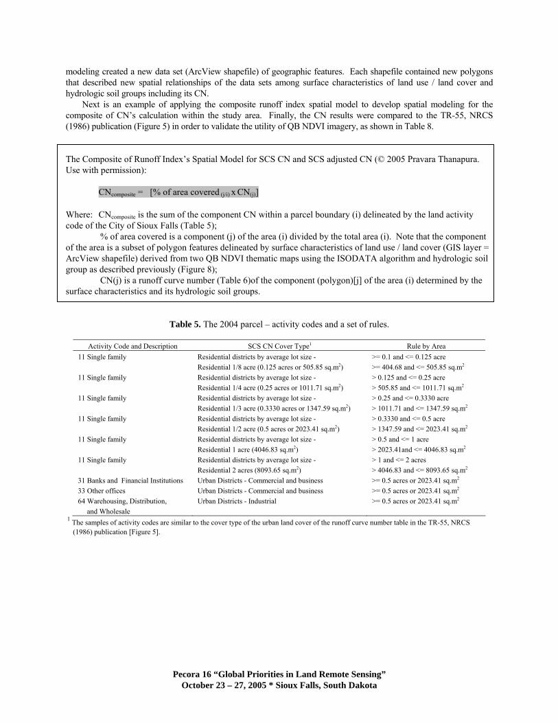
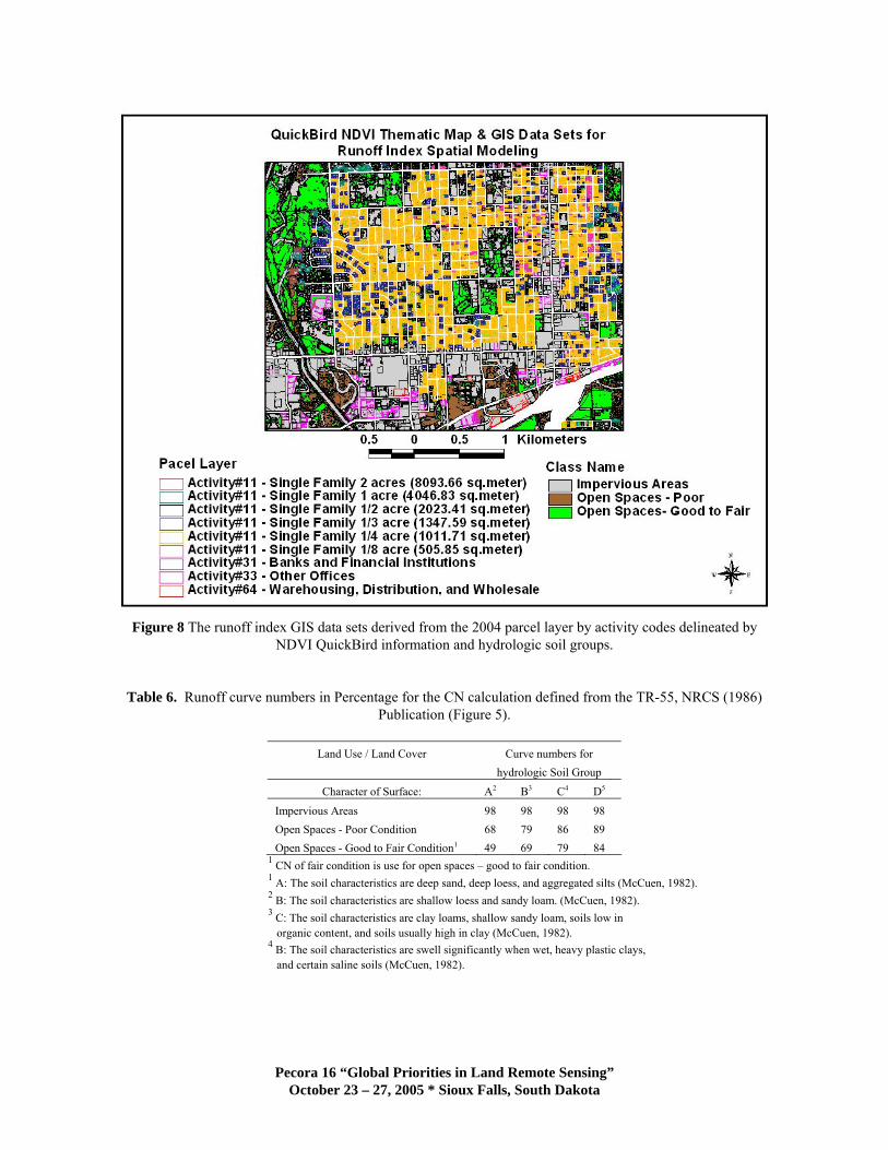

Table 8 The CN Results and SCS CN comparison
GIS Activity Code SCS CN Cover Type1 Rule Samples Total CNID and by Area Areas2 Result
Description (avg) B3 Sample Area4
1 11 Single family Residential districts by average lot size - gt= 01 and lt= 0125 acres 312 3555 acres 8688 85 9994Residential 18 acre gt= 40468 and lt= 50585 sqm2 14386463 sqm2
(0125 acres or 50585 sqm2) 123 2 11 Single family Residential districts by average lot size - gt 0125 and lt= 025 acres 3284 5766 acres 8430 75 9976
Residential 14 acre gt 50585 and lt= 101171 sqm2 23333993 sqm2
(025 acres 101171 sqm2) 1987 3 11 Single family Residential districts by average lot size - gt 025 and lt= 03330 acres 357 10006 acres 8244 72 10000
Residential 13 acre gt 101171 and lt= 134759 sqm2 40492530 sqm2
(03330 acres 134759 sqm2) 345 4 11 Single family Residential districts by average lot size - gt 03330 and lt= 05 acres 140 5451 acres 8203 70 10000
Residential 12 acre gt 134759 and lt= 202341 sqm2 22059243 sqm2
(05 acres 202341 sqm2) 188 5 11 Single family Residential districts by average lot size - gt 05 and lt= 1 acres 43 261 acres 7684 68 9557
Residential 1 acre (404683 sqm2) gt 202341and lt= 404683 sqm2 10562213 sqm2
09 6 11 Single family Residential districts by average lot size - gt 1 and lt= 2 acres 4 456 acres 8527 65 10000
Residential 2 acres (809365 sqm2) gt 404683 and lt= 809365 sqm2 1845352 sqm2
016 7 31 Banks and Urban Districts - Commercial gt= 05 acres 17 1496 acres 9419 92 10000
Financial and business gt= 202341 sqm2 6054050 sqm2
Institutions 052 8 33 Other offices Urban Districts - Commercial gt= 05 acres 56 6396 acres 9321 92 10000
and business gt= 202341 sqm2 25883493 sqm2
22 9 64 Warehousing Urban Districts - Industrial gt= 05 acres 11 2004 acres 8631 88 9400
Distribution and gt= 202341 sqm2 8109837 sqm2
Wholesale 07 4224 89634 acres 8572 79 9881
362733112 sqm2
3089
SCS CNHydrologic Soil Group
Total
1 The samples of activity codes are similar to the cover type of the urban land cover of the runoff curve number table in the TR-55 NRCS (1986) publication [Figure 5] 2 The study area is 290142 acres (11742 hectares) 3The total area of hydrologic soil group B of each sample layer by parcel - activity code 4 B The soil characteristics are shallow loess and sandy loam (McCuen 1982)
RESULTS amp DISCUSSION
The overall accuracy of the two QB NDVI thematic maps produced is presented in Table 3 and Table 4 using classification schemes from Table 1 and Table 2 respectively Figure 6 and 7 shows the two NDVI QuickBird thematic maps with the highest overall classification accuracy used as a GIS input into the Sioux Falls spatial modeling for the composite of CNs calculations
Table 3 shows the overall accuracy results of mapping impervious areas and open spaces obtained from five different labeling criteria when the same unsupervised image of 100 spectral clusters was used The Map ID13 with the combination labeling criteria of impervious areas (DNs range between 1-50) and open spaces (DNs range between 51-100) achieved the highest overall Kappa value of 09003 with the overall classification accuracy of 9505 Comparing the accuracy results to the accuracy results obtained from other labeling criteria showed slightly differing classification accuracy improvement increasing toward the mid DNs of QB NDVI This pattern of change in classification accuracy showed the potential correlations between increasing and decreasing of the DNs and amounts of open spaces (vegetative areas) and impervious areas (non vegetative areas) [Figure 4] The DNs range from 126 to 0 indicates increasing impervious surfaces shown in shades of dark tones The DNs range from 126 to 255 indicates increasing openspaces shown in shades of light tones
Pecora 16 ldquoGlobal Priorities in Land Remote Sensingrdquo October 23 ndash 27 2005 Sioux Falls South Dakota
Table 4 shows the overall accuracy results of mapping two classes obtained from two different labeling criteria utilizing the same unsupervised image of 50 spectral clusters The overall Kappa value for the Map ID 21 and Map ID22 produced was only 044 and 045 respectively The results showed that the spectral classifications were not spectrally distinct among open spaces-poor and good-to-fair conditions Map ID21 was used in this study since its producer and user accuracy in percentages were similar which indicated higher map accuracy compare to Map ID22
Comparing the overall accuracy of the two thematic maps demonstrated using the labeling pixel criteria with the DNs 5050 spectral cluster thresholds for assigning labels into two classes was the best method to use This tended to improve classification accuracy with high Kappa values and similar percentages of producer and user accuracy
Finally the average CN values of different land use land cover descriptions covering homogeneous soil types were calculated and compared to the SCS CN The results of this comparison are shown in Table 8 in order to validate the utility of QB NDVI imagery for CN calculation The overall average CN covering approximately 30 of the study area produced was 85 and the average SCS CN was 79 Comparing CN value within GIS ID produced from different approaches demonstrated that the new design technological methodologies produced conservative CN results similar to those found in the SCS CN table
The finer resolution imagery used in this study allows for better discrimination in land use land cover and the accuracy results validate the hypothesis of this study This is reflected in the fact that overall accuracy for the two QB NDVI thematic maps produced was 95 and 73 respectively Additionally the average CN values among the GIS ID samples described as single family showed that decreasing average lot size produced higher CN numbers or higher runoff This indicates increasing amounts of impervious areas and decreasing amounts of green vegetation as expected
CONCLUSIONS
This applied research demonstrated that the proposed spatial modeling utilizing the fine spatial resolution remotely sensed data and a GIS approach were successful in accurately automating and mapping land use land cover surface characteristics and determining the runoff curve number in the urban hydrology for small watersheds Therefore the hypothesis of this study was accepted Mapping fine spatial resolution QuickBird NDVI imagery generated using the traditional unsupervised classification was a more accurate simpler and efficient data extraction approach that increased speed and potentially reduces costs of both the analysis and mapping process The application of this approach could be beneficial to municipal engineers involved with designing or maintaining stormwater management systems and drainage improvement projects
ACKNOWLEDGEMENTS
The author would like to thank the following employees of the City of Sioux Falls South Dakota for their contribution to the success of this research project Steve Van Aartsen GIS supervisor and his staff for all the data and information contributed for this project Jeff Dunn City Drainage Engineer for his time and the literature provided on hydrology in Sioux Falls and Sam Trebilcock Transportation Planner for his assistance and interest
The author would also like to thank the co authors for their support input effort and specialized expertise in making this project a success Additional thanks go to Mr Kevin Dalsted Director Engineering Resource Center South Dakota State University Brookings South Dakota for the use of the hardware and software that made this research possible
Pecora 16 ldquoGlobal Priorities in Land Remote Sensingrdquo October 23 ndash 27 2005 Sioux Falls South Dakota
REFERENCES
Bondelid TR TJ Jackson and RH McCuen 1982 Estimating runoff curve numbers using remote sensing data Singh Vijay P editor Applied modeling in catchment hydrology Water Resources Publications Littleton Colorado 563 p
Congalton R and K Green 1999 Assessing the Accuracy of Remotely Sensed Data Principles and Practices CRCLewis Press Boca Raton Florida 137 p
Chen DM and D Stow 2003 Strategies for integrating information from multiple spatial resolutions into land-use land-cover classification routines Photogrammetric Engineering amp Remote Sensing 69(11)1279-1287
Draper S E and S G Rao 1986 Runoff prediction using remote sensing imagery Water Resources Bulletin 22(6) 941-949 p
Dubayah R O E F Wood E T Engman K P Czajkowski M Zion and Rhoads 2000 Remote Sensing in Hydrology and Water Management Remote Sensing in Hydrology and Water Management Schultz G A and ET Engman editors Springer Germany 483 p
Engman E T 1982 Remote sensing applications in watershed modeling Applied modeling in catchment hydrology Singh Vijay P editor Water Resources Publications Littleton Colorado 563 p
Engman E T 1993 Remote Sensing Handbook of Hydrology Maidment David R editor New York McGraw- Hill 241-2423 p
Environmental Systems Research Institute Staff 1995 Understanding GIS Version 7 for UNIX and Open VMS John Wiley ampSons New York NY 500 p
Golding B L 1997 Discussion Runoff Curve Number Has It Reached Maturity Journal of Hydrologic Engineering 2(3) 145-148 p
Jackson T J and R M Ragan 1977 State-of-the-art application of Landsat data in urban hydrology International symposium on urban hydrology hydraulics and sediment control University of Kentucky Lexington Kentucky 275-285 p
McCuen R H 1982 A guide to hydrologic analysis using SCS methods NJ Prentice-Hall Englewood Cliffs NJ 145 p
McCuen R H 2002 Approach to confidence interval estimation for curve numbers Journal of Hydrologic Engineering 7(1) 43-48 p
McCuen R H 2003 Discussion of Approach to Confidence Interval Estimation for Curve Numbers Journal of Hydrologic Engineering 8(4) 232-233 p
McCuen R H and O Okunola 2002 Extension of TR-55 for Microwatersheds Journal of Hydrologic Engineering 7(4) 319-325 p
Melesse A M and W D Graham 2004 Storm runoff prediction based on a spatially distributed travel time method utilizing remote sensing and GIS Journal of the American Water Resources Association (JAWRA) 40(4) 863-879 p
Mishra S K and V P Singh 2003 Soil Conservation Service Curve Number (SCS-CN) methodology The Netherlands Kluwer Academic Publishers PO Box 17 3300 AA Dordrecht 536 p
Natural Resources Conservation Service (NRCS) 1972 SCS National Engineering Handbook Section 4 Hydrology URL httpwwwinfousdagovCEDftpCEDneh630-ch10pdf US Department of Agriculture Natural Resources Conservation Service (last date accessed 21 August 2005)
Natural Resources Conservation Service (NRCS) 1986 Urban hydrology for small watersheds TR-55 Technical release 55 URL httpwwwwccnrcsusdagovhydrohydro-tools-models-tr55html US Department of Agriculture National Water and Climate Water (last date accessed 21 August 2005)
Natural Resources Conservation Service (NRCS) 1992 Computer program for project formulation-hydrology Tech Release No 20 URL httpwwwwccnrcsusdagovhydrohydro-tools-models-tr20html US Department of Agriculture National Water and Climate Water (last date accessed 21 August 2005)
Ponce V M and R H Hawkins 1996 Runoff curve number has it reached maturity Journal of Hydrologic Engineering 1(1) 11-19p
Ragan R M and T J Jackson 1980 Runoff synthesis using Landsat and SCS model Journal of Hydraulics division Proceedings of the American Society of Civil Engineers (ASCE) 106(5) 667-678p
Schultz G A 1988 Remote sensing in Hydrology Journal of Hydrology 100(1-3) 239-265 p
Pecora 16 ldquoGlobal Priorities in Land Remote Sensingrdquo October 23 ndash 27 2005 Sioux Falls South Dakota
Schultz G A 1996 Remote sensing applications to hydrology Runoff Hydrological Sciences Journal 41(4) 453-475 p
Thomas J J and R H McCuen 1979 Accuracy of impervious area values estimated using remotely sensed data Water Resources Bulletin 27(3) 373-379 p
Pecora 16 ldquoGlobal Priorities in Land Remote Sensingrdquo October 23 ndash 27 2005 Sioux Falls South Dakota
- ABSTRACT
- METHODS
- Study Area
- Digital Data amp Pre-Processing
- Classification Approach
-
- REFERENCES
-
Mapping Urban Land Use Land Cover Using QuickBird NDVI Imagery for Runoff Curve Number Determination
Pravara Thanapura Engineering Resource Center
Suzette Burckhard Civil and Environmental Engineering
Mary Orsquo Neill Engineering Resource Center
Dwight Galster and Mathematics and Statistics
South Dakota State University Brookings
South Dakota 57007 USA
Eric Warmath
Department of Transportation State of Nevada
1263 S Stewart Street
Carson City Nevada 89712 USA
ABSTRACT
The objective of this study was to evaluate Normalized Difference Vegetation Index (NDVI) data derived from QuickBird (QB) satellite imagery to map impervious areas and open spaces for runoff curve number (CN) determination The image was collected on April 26 2004 and provided by the City of Sioux Falls SD The image was radiometrically and geometrically corrected prior to this study The imagery has four bands (including the blue green red and near-infrared) and was imaged at a 239-meter spatial resolution The red channel (band 3 630-690 nm) and the near infrared channel (band 4 760-900 nm) were used to create the QB NDVI dataset (Band 4 - Band3 Band 4 + Band3) This research employed the urban land cover classification scheme of the runoff curve number table in the TR-55 (NRCS 1986) publication An unsupervised spectral classification approach was used in this study The research hypothesis was that high-resolution NDVI could improve the efficiency and effectiveness of urban land cover data extraction For the accuracy assessment process a simple random sampling scheme was employed using a random number generator to select points from the classified QB NDVI imagery for comparison to the 06-meter spatial resolution orthoimage acquired on April 23 2004 The overall and individual Kappa coefficients were calculated The overall accuracy for the two QB NDVI thematic maps produced was 95 and 73 respectively The average CN values of homogeneous land use land cover and soil type covering approximately 30 of the study area were determined and compared to the SCS CN in order to validate the utility of QB NDVI imagery for CN calculation The overall average CN produced from the spatial modeling was 85 and the average SCS CN was 79
INTRODUCTION
Remote satellite sensing application in hydrology did not start until the first launch of Earth Resources Technology Satellite (ERTS) [later renamed Landsat 1] in July of 1970 QUOTE (Schultz 1988) (Schultz 1988) Remotely sensed data is rapidly becoming an important source of information in hydrologic modeling monitoring and research QUOTE (Engman 1982 Engman 1993 Melesse and Graham 2004) (Engman 1982 1993 Melesse and Graham 2004) QUOTE ADDIN PROCITE yuml1105lsquo190200000000010000)030000F5C_Procite5CPravara_Thanapura1pdt10Engman 1982 8100102000600agraveagrave000000iquestH00agrave1400yumlyumlyumlyuml00000000010000001400000001000000000000000A000000000000ordmI_˜lsaquoEuml00010000000100000000000000tograve12000notW00yumlyumlyumlyuml QUOTE ADDIN PROCITE yuml1105lsquo190200000000010000F030000F5C_Procite5CPravara_Thanapura1pdt1AMelesse amp Graham 2004 8450104000700agraveagrave000000iquestH00 7140014000000010000000000000000000000100000000000000003000000000000AtildeAcircw00000000yumlyumlyumlyuml07AumlAcircwTHORNAcircAcircw0000200uumlntilde1200atildeAcircAcircw0600agraveagrave000000iquestH00 714001400000001000000000000000000000010000000000000000A000000000000ordmI_hUgraveEuml00030000000500000000000000tograve12000notW00yumlyumlyumlyuml Its advantages include spectral radiometric spatial and temporal resolutions including its ability to generate information and to provide a means of observing hydrological state variables over large areas or small complex basins It offers an alternative to conventional data collection employed in the estimation of certain hydrologic model parameters The primary benefits obtainable from using remote sensing are the reduction of manpower time and monetary resources required for data collecting and processing For some situations remote sensing provides information that was previously impossible or impractical to obtain using conventional techniques QUOTE (Thomas and McCuen 1979) (Thomas and McCuen 1979) Therefore remote sensing technology is a very important tool for successful hydrologic model analysis prediction and validation The National Resource Conservation Service (NRCS) formally the Soil Conservation Service (SCS) has developed a series of hydrologic models in water resource planning and design The SCS Curve Number (SCS-CN) method is the best-known component of the SCS hydrologic models According to Ponce and Hawkins (1996) the origins of the CN methodology can be traced back to the thousand of infiltrometer tests carried out by SCS in the late 1930s and early 1940s The intent was to develop basic data to evaluate the effects of watershed treatment and soil conservation measures on the rainfall-runoff process A major catalyst for the development and implementation of the runoff CN methodology was the passage of the Watershed Protection and Flood Prevention Act (Public Law 83-566) in August 1954 The method and its use are described in the SCS National Engineering Handbook Section 4 Hydrology (NEH-4) QUOTE (Soil Conservation Service (SCS) 1972) [NRCS 1972] The document has since been revised in 1956 64 65 71 72 85 and 1993 The CN method is well established in hydrologic engineering and environmental impact analyses Its major advantage are (1) its simplicity (2) its predictability (3) its stability (4) its reliance on only one parameter and (5) its responsiveness to major runoff-producing watershed properties (soil type land covertreatment surface condition and antecedent condition) [ QUOTE (Ponce and Hawkins 1996) Ponce and Hawkins 1996] Consequently the methodology has been widely used in numerous applications by practicing engineers and hydrologists nationally and internationally QUOTE (McCuen 1982 Ponce and Hawkins 1996 Golding 1997 McCuen 2002 McCuen and Okunola 2002 Mishra and Singh 2003 McCuen 2003) (McCuen 1982 2002 2003 Ponce and Hawkins 1996 Golding 1997 McCuen and Okunola 2002 Mishra and Singh 2003) QUOTE ADDIN PROCITE yuml1105lsquo19020000000001000012030000F5C_Procite5CPravara_Thanapura1pdt11Golding 1997 7870102000700agraveagrave0C0000iquestH00xB1400yumlyumlyumlyuml00000000010000001400000001000000000000000A000000000000ordmI_Agrave08Ccedil00030000000500000000000000umlograve12000notW00yumlyumlyumlyuml QUOTE ADDIN PROCITE yuml1105lsquo19020000000001000013030000F5C_Procite5CPravara_Thanapura1pdt19Ponce amp Hawkins 1996 7880104000500agraveagrave000000iquestH00agrave1400yumlyumlyumlyuml000000000100000014000000010000000000000003000000000000002000000000019notAcircw00000000yumlyumlyumlyumlFnotAcircw000000003laquoAcircw0700agraveagrave000000iquestH00agrave1400yumlyumlyumlyuml00000000010000001400000001000000000000000A000000000000ordmI_deg0BIacute00030000000500000000000000umlograve12000notW00yumlyumlyumlyuml QUOTE ADDIN PROCITE yuml1105lsquo19020000000001000015030000F5C_Procite5CPravara_Thanapura1pdt10McCuen 2003 7900102000600agraveagrave000000iquestH00xB1400yumlyumlyumlyuml00000000010000001400000001000000000000000A000000000000ordmI_deg0BIacute00050000000500000000000000umlograve12000notW00yumlyumlyumlyuml QUOTE ADDIN PROCITE yuml1105lsquo1902000000000100001E030000F5C_Procite5CPravara_Thanapura1pdt1AMcCuen amp Okunola 2002 7990104000600agraveagrave000000iquestH00xB1400yumlyumlyumlyuml000000000100000014000000010000000000000003000000000000002000000000019notAcircw00000000yumlyumlyumlyumlFnotAcircw000000003laquoAcircw0700agraveagrave000000iquestH00xB1400yumlyumlyumlyuml00000000010000001400000001000000000000000A000000000000ordmI_deg0BIacute00050000000500000000000000umlograve12000notW00yumlyumlyumlyuml QUOTE ADDIN PROCITE yuml1105lsquo190200000000010000$030000F5C_Procite5CPravara_Thanapura1pdt10McCuen 1982 8050102000600agraveagrave000000iquestH00agrave1400yumlyumlyumlyuml00000000010000001400000001000000000000000A000000000000ordmI_08Ecirc00010000000100000000000000umlograve12000notW00yumlyumlyumlyuml QUOTE ADDIN PROCITE yuml1105lsquo1902000000000100006030000F5C_Procite5CPravara_Thanapura1pdt18Mishra amp Singh 2003 8230104000600agraveagrave000000iquestH00agrave1400yumlyumlyumlyuml000000000100000014000000010000000000000003000000000000002000000000019notAcircw00000000yumlyumlyumlyumlFnotAcircw000000003laquoAcircw0500agraveagrave000000iquestH00agrave1400yumlyumlyumlyuml00000000010000001400000001000000000000000A000000000000ordmI_08Ecirc00010000000100000000000000umlograve12000notW00yumlyumlyumlyuml
The CN is an index that represents the combined hydrologic effect of soil group land cover type agricultural land treatment class hydrologic condition and antecedent soil moisture QUOTE (McCuen 1982) (McCuen 1982) It is the best-known component of a series of SCS hydrologic models most noticeably the TR-55 QUOTE (Natural Resources Conservation Service (NRCS) 1986) (NRCS 1986) QUOTE Natural Resources Conservation Service United States Department of Agriculture 1986 822 procedures and the TR-20 computer model QUOTE (Natural Resources Conservation Service (NRCS) 1984 McCuen 2002) (NRCS 1992 McCuen 2002) QUOTE ADDIN PROCITE yuml1105lsquo19020000000001000011030000F5C_Procite5CPravara_Thanapura1pdt10McCuen 2002 7860102000600agraveagrave000000iquestH00agrave1400yumlyumlyumlyuml00000000010000001400000001000000000000000A000000000000ordmI_pograveEacute00050000000500000000000000umlograve12000notW00yumlyumlyumlyuml The CN calculation requires use of storm rainfall and associated streamflow data for annual floods to derive the best means of establishing run off curve numbers A CN of 100 represents a condition of zero potential retention or 100 runoff of incident precipitation
Determination of the CN has been traditionally a time-consuming and labor-intensive procedure A basic problem exists in quantifying detailed spatial extent and distribution of various land cover classes Therefore remote sensing technology has become one of the primary methods for acquiring land cover data for providing detailed mapping information as input into the CN method (Jackson and Ragan 1977 Engman 1982 1993 Draper and Rao 1986 Schultz 1996 Dubavah et al 2000)
In previous studies one of the main problems of using remotely sensed data for estimation of land cover is a spatial resolution issue Moderate spatial resolutions are insufficient to generate the detail necessary to utilize the published SCS land cover table used in the SCS procedures Egrave008000000010000000000200atilde120080000000500agraveagrave00000005lsquo|yumlyumlyumlyumlm05lsquo|THORNAcircAcircw0000010007000000`00000080000000500000000000005lsquo|yumlyumlyumlyumlm05lsquo|THORNAcircAcircw0000010007000000`00000080000000700agraveagrave00000005lsquo|yumlyumlyumlyumlm05lsquo|THORNAcircAcircw0000010007000000`000000800000007000000000000AtildeAcircw000020000000000IcircAtildeAcircw00000000yumlyumlyumlyuml07AumlAcircw0000000600agraveagrave00000005lsquo|0000200m05lsquo|THORNAcircAcircw0000010007000000latilde1200800010007000000000000AtildeAcircw000020000000000IcircAtildeAcircw00000000yumlyumlyumlyuml07AumlAcircw80000000600agraveagrave00000005lsquo|0000200m05lsquo|THORNAcircAcircw0000010007000000latilde1200800010006000000000000AtildeAcircw000020000000000IcircAtildeAcircw00000000yumlyumlyumlyuml07AumlAcircw8000000020000F5C_Procite5CPravara_Thanapura1pdt19Ragan amp Jackson 1980 6420104000500agraveagrave000000iquestH00agrave1400yumlyumlyumlyuml000000000100000014000000010000000000000003000000000000002000000000019notAcircw00000000yumlyumlyumlyumlFnotAcircw000000003laquoAcircw0700agraveagrave000000iquestH00agrave1400yumlyumlyumlyuml00000000010000001400000001000000000000000A000000000000ordmI_08Ecirc00010000000100000000000000umlograve12000notW00yumlyumlyumlyuml QUOTE (Ragan and Jackson 1980 Engman 1982 Engman 1993) (Ragan and Jackson 1980 Engman 1982 1993) QUOTE ADDIN PROCITE yuml1105lsquo190200000000010000 030000F5C_Procite5CPravara_Thanapura1pdt10Engman 1993 8010102000600agraveagrave000000iquestH00agrave1400yumlyumlyumlyuml00000000010000001400000001000000000000000A000000000000ordmI_08Ecirc00010000000100000000000000umlograve12000notW00yumlyumlyumlyuml QUOTE ADDIN PROCITE yuml1105lsquo190200000000010000)030000F5C_Procite5CPravara_Thanapura1pdt10Engman 1982 8100102000600agraveagrave000000iquestH00agrave1400yumlyumlyumlyuml00000000010000001400000001000000000000000A000000000000ordmI_08Ecirc00010000000100000000000000umlograve12000notW00yumlyumlyumlyuml Engman in 1982 and 1993 suggested that one must develop a land cover table analogous that is compatible to the Landsat data Landsat may not be acceptable in small areas with certain land cover types Bondelid et al (1982) stated that special care should be exercised in analyzing small watersheds that contain heterogeneous land cover causing the largest CN errors Engineering designs utilizing the curve number are widely used but the curve number is sensitive to errors in the estimated input values used to derive it QUOTE (Bondelid et al 1982) (Bondelid et al 1982 McCuen 2002)
Remote sensing GIS GPS and image processing technological capability have improved significantly since the previous studies Commercial high-resolution satellite imagery creates unique opportunities to address and potentially solve old problems The purpose of this applied research is to bridge remote sensing and GIS to produce scientific knowledge by designing technological methodologies for determining the composite of curve numbers in the urban hydrology for small watersheds technical release 55 (TR-55) table NRCS (1986) publication for practicing professionals in urban water resource planning The theoretical foundation is that mapping a high resolution NDVI image generated using the ISODATA algorithm is an efficient and effective information extraction approach for the composite of runoff curve number calculation
METHODS
In this research newly designed technological methodologies were proposed for mapping urban land use land cover using QuickBird NDVI imagery and developing GIS spatial modeling for generating the composite of curve numbers in the TR-55 table NRCS (1986) publication To achieve this goal a sequence for digital processing and analysis was proposed and implemented (Figure 1) In order to assess the utility of QB NDVI imagery and to validate the composite runoff curve number calculation using designed GIS spatial modeling various procedures and comparisons of the generated runoff coefficients were presented reviewed and validated by practicing professionals including the City Drainage Engineer and the City Geographic Information Systems manager for the City of Sioux Falls South Dakota in August 2005
Figure 1 Sequence for digital processing and analysis
Study Area
The City of Sioux Falls is located in southeastern South Dakota Sioux Falls covers 40208 acres (162716 hectares) and has a population of approximately 138000 Climatologically Sioux Falls is in a continental climate with an average rainfall of 2386 inches (606 cm) and approximately 40 inches (1016 cm) of snow annually The majority of the precipitation comes in spring and summer with May and June being the months of maximum precipitation for the region The study area for this project is centered on 43O 31rsquo 18rdquo north latitude and 96O 44rsquo 42rsquorsquo west longitude in the southwestern part of the city This area encompasses 290142 acres (11742 hectares) with various land use land cover types and includes all or part of 26 hydrological urban sub-basins (Figure 2)
(a) (b)
Figure 2 The 2004 images of the study area at the same scale(a) The QuickBird multi image (4-3-2) on the left and (b) The QuickBird NDVI image on the right
Digital Data amp Pre-Processing
The 2004 remotely sensed data and vector GIS data layers were provided by the City of Sioux Falls They include orthophoto mosaics with 2 ft (06 m) and 05 ft (015 m) resolution a QuickBird satellite image with 796 ft (239 m) resolution and include data layers such as parcels city limit boundary hydrography and streets The data sets were processed and merged to combine the remotely sensed data with the GIS layers for the study area The April 23 2004 orthophoto was used as a reference to integrate all data sets into the same map projection and unit with the Universal Transverse Mercator (UTM) map projection World Geodetic System (WGS) 1984 and horizontal units in feet Software used in this project consisted of ERDAS Imagine 87 ArcMap 9 ArcView 33 and Microsoft Excel 2002
The two digital orthophotographs were acquired on April 23 2004 and May 20 2002 respectively Both orthophotos were collected and scanned to meet the combined requirements of National Map Accuracy Standards 90 of all contours will be within frac12 contour interval and 90 of horizontal positions shall be within 130 of one inch at the specified map scale The specified horizontal map scale was 1 inch = 200 ft (609m) The flight height above terrain was 4000 ft (12192m) for a photo negative scale of 1 inch = 667 ft (2033m) Contour interval for the elevation data was 2 ft (061m) The radiometric density of the digital orthophotograph was 10 bits per channel with a geometric precision of 1 micron Both orthophotos were provided in UTM projection WGS84 datum and planar distance survey units in feet Additionally both orthophotos were subset to the study area and the 2002 orthophoto was degraded 3x3 using ERDAS Imagine 87 Overlaying of the subset orthophotos demonstrated good alignment between images Therefore an image to image registration was not required
The QuickBird leaf-on image was collected on April 26 2004 The image was radiometrically corrected and orthorectified prior to this study with UTM projection WGS84 datum and units in meters The imagery has four bands (including the blue green red and near-infrared) and was imaged at a 239-meter spatial resolution in unsigned 16 bit data type The subset QB image was created in unsigned 8 bit data type The image was observed with no signs of atmospheric contamination The statistical spectral information showed a normal distribution with similar mean median and mode values Geometric correction was performed The subset scene was registered to the 2004 orthophoto with 31 ground control points and the RMS was 06940 pixel Figure 3 demonstrates the result The red channel (band 3 630-690 nm) and the near infrared channel (band 4 760-900 nm) were processed to create the QB NDVI image (NDVI = Band 4 - Band3 Band 4 + Band3) in unsigned 8 bit data type for the study area
The 2004 NRCS SSURGO 124000 data set of the soil survey area (SSA) named ldquoMinnehaha County South Dakotardquo and its standard metadata files were downloaded from the Soil Data Mart at on June 7 2004 It is a digital soil survey and generally is the most detailed level of soil geographic data developed by the National Cooperative Soil Survey The soil layer was in a single zip file in ArcView shapefile format with a geographic coordinate system and using North American Datum (NAD) 1983 This layer was processed using ArcView 33 geoprocessing and Microsoft Excel 2002 to create a soil layer associated with hydrologic soil groups in the project coordinate system for this study area Overlaying of the soil hydro features to the subset QB image demonstrated a good fit Therefore a vector to image registration was not necessary
(a) (b)
Figure 3 The registered 2004 images comparison at same scale and location
(a) The QuickBird multi image (4-3-2) on the left with the 2004 Orthoimage (1-2-3) on the right
(b) The QuickBird NDVI image on the left with the 2004 Orthoimage (1-2-3) on the right
Classification Approach
With the recent development of new remote sensing systems there are an increasing number of commercially high resolution data available There is a considerable amount of previous research that has been devoted to exploring the magnitude and impact of spatial resolution on image analysis when changing scale from coarse to fine resolutions Due to the more heterogeneous spectral-radiometric characteristics within land use land cover unit portrayed in high resolution images many applications of traditional single-resolution classification approaches have not led to satisfactory results In general traditional single-resolution classification procedures such as supervised unsupervised and hybrid training approaches are inadequate for discriminating between land use land cover classes where spectralspatial features and spatial patterns vary as a function of spatial resolution Consequently there is an increasing need of researching for more efficient approaches to process and analyze these data products (Chen and Stow 2003)
In this research the relatively simple Normalized Difference Vegetation Index (NDVI) was introduced in order to reduce heterogeneous spectral-radiometric characteristics within land use land cover surfaces portrayed in high resolution images It also was used for improving the accuracy level of details for mapping impervious surfaces and open spaces with different hydrologic conditions as used in the proposed SCS runoff curve number (CN) calculation in this study Additionally this research presented applying the principle behind NDVI using high spatial resolution QuickBird imagery based on the unique interaction differences in land use land cover surfaces with reflected or emitted electromagnetic radiation between QB Red band (630-690nm) and QB NIR band (760-900nm)
NDVI has been shown to correlate green leaf biomass and green leaf area index Chlorophylls the primary photosynthetic pigments in green plants absorb light primarily from the red and blue portions of the spectrum while a higher proportion of infrared is reflected or scattered As a result vigorously growing healthy vegetation has low red-light reflectance and high near-infrared reflectance and hence high NDVI values Impervious surfaces (eg Asphalt concrete buildings etc) and bare land (eg bare soil rock dirt etc) have similar reflectance in the red and the near infrared so these surfaces will have values near zero NDVI is calculated using the formula (Near infrared ndash red)(Near infrared + red) This relatively simply algorithm produces output values in the range of -10 to 10
Figure 4 shows a visual comparison of spectral correlation between QuickBird NDVI in unsigned 8 bit data type (0-255) for impervious areas and open spaces in the urban environment The impervious surfaces are the dark areas with low NDVI DNs and the brighter areas are vegetative covers with high NDVI DNs
(a) The 2004 QuickBird NDVI (b) The QuickBird multi image (4-3-2)
(c) The 2004 Orthophoto (1-2-3)
Figure 4 The registered 2004 images visual comparison of impervious areas and vegetative open spaces at same scale and location in residential areas
This research employed the urban land cover of the runoff curve number table in the TR-55 NRCS (1986) publication (Figure 5) The classification schemes defined from the TR-55 are detailed in Table 1 and Table 2 The defined classification schemes were used to generate two QB NDVI thematic maps using the ISODATA algorithm Gaussian Maximum Likelihood Classifier with ERDAS Imagine 87 assigning unsupervised spectral classes and assessing the accuracy of the maps The detailed map information from the second thematic map was then converted as a GIS input into a spatial modeling for calculating the composite of CNrsquos using the composite runoff index spatial model below
This spatial model based on the composite of the CNrsquos equation below can be applied for calculating the runoff index for both the SCS CN method and the rational method the CN number calculated for the SCS CN method and a runoff coefficient is the ldquocrdquo value used in the rational method recommended by the American Society of Civil Engineers and the Water Pollution Control Federation
The Composite of Runoff Indexrsquos Spatial Model (copy 2005 Pravara Thanapura Use with permission)
Runoff Indexcomposite = ( [ of area covered (ji) x CN(j)]
Where
CNcomposite is the sum of the component runoff index within an area (i) delineated by description of area
of area covered (ji) is the component (j) of the area (i) divided by the total area (i) Note that the component of the area is delineated by surface characteristics of land use land cover andor hydrologic soil group
CN(j) is a runoff index of the component (j) of the area (i) determined by the surface characteristics andor its hydrologic soil groups
The Composite CNrsquos Weigh Average Equation
CNcomposite = ( [ of area covered x CN] Where CNcomposite is the sum of composite runoff curve number within an area
of area covered is a component of the area divided by the total area
CN is the runoff curve number of the area
In this study the composite of CNrsquos calculation requires the combined surface characteristics and hydrologic effect of soil groups The surface characteristic was derived from the two QB NDVI thematic maps and the hydrologic soil groups were obtained from the 2004 NRCS SSURGO 124000 data set The soil information covered by hydrologic areas such as rivers or canals are not surveyed or were not available in this data set Therefore they were excluded from the decision rules Swimming pools were considered as impervious areas since these small size water features appeared spectrally impervious on the QB NDVI Additionally they retain precipitation and act as pervious surfaces during storms thus the decision rules would result in a conservative calculation of CNrsquos
There is one heavy industrial area in the southern part of the study area This area was an oil and fuel storage facility The tanks and their associated grass covered containment areas approximately 038 of the study areas 290142 acres (11742 hectares) The tank structures themselves were impervious but they were spectrally ruled as open spaces which resulted in a conservative composite CN calculation Precipitation falling on the containment areas does not interact with the surface and groundwater since precipitation falling in these areas evaporates naturally or is pumped out and treated as wastewater
Figure 5 TR-55 runoff curve number table for urban areas 14001400000001000000000000000000000010000000000000000A000000000000ordmI_cedil13Eacute00030000000500000000000000tograve12000notW00yumlyumlyumlyuml QUOTE (United States Department of Agriculture 1986) (United States Department of Agriculture 1986)
Table 1 Initial land use land cover classification scheme of QuickBird NDVI thematic map1 (Figure 6)[copy 2005 Pravara Thanapura Use with permission]
Table 2 Secondary land use land cover classification scheme of QuickBird NDVI thematic map2 (Figure 7)
[copy 2005 Pravara Thanapura Use with permission]
Sampling Design amp Accuracy Assessment
A simple random sampling method was chosen to ensure unbiased sample selection To provide a statistically sound assessment of accuracy the simplified worst-case scenario equation was used to calculate the sample sizes to insure sufficient samples for filling in an error matrix for this project
The Conservative Sample Size Equation (Congalton and Green 1999)
n = B 4b2
Where
n = Total samples of all classes
B = The upper (αk) x 100th percentile of the Chi-Squared distribution with 1 degree of freedom (α) k = number of classes
b = Significant level = +- 5 accuracy (α - 095 = 005)
Over 500 sample points were generated for each thematic map using the ISODATA algorithm to insure good distribution across the study area Figure 6 and 7 show the accuracy assessment sites acquired for the entire classification of each QB NDVI thematic map To accomplish this ERDAS 87rsquos random number generator function was used to create random points from the QB NDVI thematic maps for comparison to the 2004 2 ft (06 m) and the 2002 05 ft (015 m) spatial resolution orthophotos The program automatically discarded random points not sufficiently representing relatively homogenous areas This function minimized registration errors of the image and helped to accurately interpret a true representation of each reference point on the orthophoto To assure visual interpretation consistency these reference points were individually evaluated by one team member with many years of photo interpretation experience In some cases there were conflicts due to lsquoleanrsquo in the orthophoto or mixed pixels around the edges These points were re-evaluated using the 2004 orthophoto Quality control was performed on the data set by the principal author Finally the error matrixes were generated and the overall and individual Kappa coefficients were calculated (Table 3 and 4)
Figure 6 Classification result of NDVI QuickBird thematic map 1and 502 accuracy sites
Figure 7 Classification result of NDVI QuickBird thematic map 2 and the accuracy assessment sites
Table 3 Accuracy assessment result of NDVI QuickBird thematic map1
Labeling spectral clusters the lower the numbers the darker the areas are label to impervious areas (low NDVI value)
Labeling spectral clusters the higher the numbers are the brighter the areas are label to open spaces (high NDVI value)
Table 4 Accuracy assessment result of NDVI QuickBird thematic map2
Labeling spectral clusters the lower the numbers the darker the areas are label to open spaces-poor condition (low NDVI value)
Labeling spectral clusters the higher the numbers the brighter the areas are label to open spaces-good to fair condition (high NDVI value)
GIS Spatial Modeling
A spatial modeling or analysis is a set of analytical procedures applied with a GIS A spatial model is a set of clearly defined analytical procedures that run on a spatial database to derive new information describing a new spatial relationship It is structured as a set of rules including a combination of logical expressions mathematical procedures and criteria built using analytical tools in GIS which are applied for the purpose of simulating the process QUOTE (Environmental Systems Research Institude 1995) (ESRI staff 1995)
In GIS there are three categories of spatial modeling functions that can be applied to geographic data objects (1) geometric models such as calculating the Euclidean distance between objects generating buffers calculating areas and perimeters and so on (2) coincidence models such as polygon overlay and (3) adjacency models (pathfinding redistricting and allocation) All three model categories support operations on geographic data objects such as points lines polygon TINS and grids QUOTE (Environmental Systems Research Institude 1995) (ESRI staff 1995)
In this study the geometric and coincidence modeling functions in ArcView33 geoprocessing were designed in a sequence of steps to build a spatial modeling based on the composite runoff index spatial model The process of spatial modeling created a new data set (ArcView shapefile) of geographic features Each shapefile contained new polygons that described new spatial relationships of the data sets among surface characteristics of land use land cover and hydrologic soil groups including its CN
Next is an example of applying the composite runoff index spatial model to develop spatial modeling for the composite of CNrsquos calculation within the study area Finally the CN results were compared to the TR-55 NRCS (1986) publication (Figure 5) in order to validate the utility of QB NDVI imagery as shown in Table 8
The Composite of Runoff Indexrsquos Spatial Model for SCS CN and SCS adjusted CN (copy 2005 Pravara Thanapura Use with permission)
CNcomposite = ( [ of area covered (ji) x CN(j)]
WhereCNcomposite is the sum of the component CN within a parcel boundary (i) delineated by the land activity code of the City of Sioux Falls (Table 5)
of area covered is a component (j) of the area (i) divided by the total area (i) Note that the component of the area is a subset of polygon features delineated by surface characteristics of land use land cover (GIS layer = ArcView shapefile) derived from two QB NDVI thematic maps using the ISODATA algorithm and hydrologic soil group as described previously (Figure 8)
CN(j) is a runoff curve number (Table 6)of the component (polygon)[j] of the area (i) determined by the surface characteristics and its hydrologic soil groups
Table 5 The 2004 parcel ndash activity codes and a set of rules
1 The samples of activity codes are similar to the cover type of the urban land cover of the runoff curve number table in the TR-55 NRCS (1986) publication [Figure 5]
Figure 8 The runoff index GIS data sets derived from the 2004 parcel layer by activity codes delineated by NDVI QuickBird information and hydrologic soil groups
Table 6 Runoff curve numbers in Percentage for the CN calculation defined from the TR-55 NRCS (1986) Publication (Figure 5)
1 CN of fair condition is use for open spaces ndash good to fair condition1 A The soil characteristics are deep sand deep loess and aggregated silts (McCuen 1982)
2 B The soil characteristics are shallow loess and sandy loam (McCuen 1982)
3 C The soil characteristics are clay loams shallow sandy loam soils low in organic content and soils usually high in clay (McCuen 1982)
4 B The soil characteristics are swell significantly when wet heavy plastic clays and certain saline soils (McCuen 1982)
Table 8 The CN Results and SCS CN comparison
GISActivity Code SCS CN Cover Type1RuleSamplesTotal CN
IDand by AreaAreas2Result
Description (avg)
B
3
Sample Area
4
111 Single familyResidential districts by average lot size - gt= 01 and lt= 0125 acres3123555 acres8688859994
Residential 18 acre
gt= 40468 and lt= 50585 sqm
2
14386463 sqm
2
(0125 acres or 50585 sqm
2
)
123
211 Single familyResidential districts by average lot size - gt 0125 and lt= 025 acres32845766 acres8430759976
Residential 14 acre
gt 50585 and lt= 101171 sqm
2
23333993 sqm
2
(025 acres 101171 sqm
2
)
1987
311 Single familyResidential districts by average lot size - gt 025 and lt= 03330 acres35710006 acres82447210000
Residential 13 acre
gt 101171 and lt= 134759 sqm
2
40492530 sqm
2
(03330 acres 134759 sqm
2
)
345
411 Single familyResidential districts by average lot size - gt 03330 and lt= 05 acres1405451 acres82037010000
Residential 12 acre
gt 134759 and lt= 202341 sqm
2
22059243 sqm
2
(05 acres 202341 sqm
2
)
188
511 Single familyResidential districts by average lot size - gt 05 and lt= 1 acres43261 acres7684689557
Residential 1 acre (404683 sqm
2
)gt 202341and lt= 404683 sqm
2
10562213 sqm
2
09
611 Single familyResidential districts by average lot size - gt 1 and lt= 2 acres4456 acres85276510000
Residential 2 acres (809365 sqm
2
)gt 404683 and lt= 809365 sqm
2
1845352 sqm
2
016
731 Banks and Urban Districts - Commercial gt= 05 acres 171496 acres94199210000
Financial and business
gt= 202341 sqm
2
6054050 sqm
2
Institutions 052
833 Other officesUrban Districts - Commercialgt= 05 acres566396 acres93219210000
and business
gt= 202341 sqm
2
25883493 sqm
2
22
964 Warehousing Urban Districts - Industrialgt= 05 acres112004 acres8631889400
Distribution and
gt= 202341 sqm
2
8109837 sqm
2
Wholesale 07
422489634 acres8572799881
362733112 sqm
2
3089
SCS CN
Hydrologic Soil Group
Total
1 The samples of activity codes are similar to the cover type of the urban land cover of the runoff curve number table in the TR-55 NRCS (1986) publication [Figure 5]
2 The study area is 290142 acres (11742 hectares)
3The total area of hydrologic soil group B of each sample layer by parcel - activity code4 B The soil characteristics are shallow loess and sandy loam (McCuen 1982)
RESULTS amp DISCUSSION
The overall accuracy of the two QB NDVI thematic maps produced is presented in Table 3 and Table 4 using classification schemes from Table 1 and Table 2 respectively Figure 6 and 7 shows the two NDVI QuickBird thematic maps with the highest overall classification accuracy used as a GIS input into the Sioux Falls spatial modeling for the composite of CNs calculations
Table 3 shows the overall accuracy results of mapping impervious areas and open spaces obtained from five different labeling criteria when the same unsupervised image of 100 spectral clusters was used The Map ID13 with the combination labeling criteria of impervious areas (DNs range between 1-50) and open spaces (DNs range between 51-100) achieved the highest overall Kappa value of 09003 with the overall classification accuracy of 9505 Comparing the accuracy results to the accuracy results obtained from other labeling criteria showed slightly differing classification accuracy improvement increasing toward the mid DNs of QB NDVI This pattern of change in classification accuracy showed the potential correlations between increasing and decreasing of the DNs and amounts of open spaces (vegetative areas) and impervious areas (non vegetative areas) [Figure 4] The DNs range from 126 to 0 indicates increasing impervious surfaces shown in shades of dark tones The DNs range from 126 to 255 indicates increasing openspaces shown in shades of light tones
Table 4 shows the overall accuracy results of mapping two classes obtained from two different labeling criteria utilizing the same unsupervised image of 50 spectral clusters The overall Kappa value for the Map ID 21 and Map ID22 produced was only 044 and 045 respectively The results showed that the spectral classifications were not spectrally distinct among open spaces-poor and good-to-fair conditions Map ID21 was used in this study since its producer and user accuracy in percentages were similar which indicated higher map accuracy compare to Map ID22
Comparing the overall accuracy of the two thematic maps demonstrated using the labeling pixel criteria with the DNs 5050 spectral cluster thresholds for assigning labels into two classes was the best method to use This tended to improve classification accuracy with high Kappa values and similar percentages of producer and user accuracy
Finally the average CN values of different land use land cover descriptions covering homogeneous soil types were calculated and compared to the SCS CN The results of this comparison are shown in Table 8 in order to validate the utility of QB NDVI imagery for CN calculation The overall average CN covering approximately 30 of the study area produced was 85 and the average SCS CN was 79 Comparing CN value within GIS ID produced from different approaches demonstrated that the new design technological methodologies produced conservative CN results similar to those found in the SCS CN table
The finer resolution imagery used in this study allows for better discrimination in land use land cover and the accuracy results validate the hypothesis of this study This is reflected in the fact that overall accuracy for the two QB NDVI thematic maps produced was 95 and 73 respectively Additionally the average CN values among the GIS ID samples described as single family showed that decreasing average lot size produced higher CN numbers or higher runoff This indicates increasing amounts of impervious areas and decreasing amounts of green vegetation as expected
CONCLUSIONS
This applied research demonstrated that the proposed spatial modeling utilizing the fine spatial resolution remotely sensed data and a GIS approach were successful in accurately automating and mapping land use land cover surface characteristics and determining the runoff curve number in the urban hydrology for small watersheds Therefore the hypothesis of this study was accepted Mapping fine spatial resolution QuickBird NDVI imagery generated using the traditional unsupervised classification was a more accurate simpler and efficient data extraction approach that increased speed and potentially reduces costs of both the analysis and mapping process The application of this approach could be beneficial to municipal engineers involved with designing or maintaining stormwater management systems and drainage improvement projects
AcknowleDgements
The author would like to thank the following employees of the City of Sioux Falls South Dakota for their contribution to the success of this research project Steve Van Aartsen GIS supervisor and his staff for all the data and information contributed for this project Jeff Dunn City Drainage Engineer for his time and the literature provided on hydrology in Sioux Falls and Sam Trebilcock Transportation Planner for his assistance and interest
The author would also like to thank the co authors for their support input effort and specialized expertise in making this project a success Additional thanks go to Mr Kevin Dalsted Director Engineering Resource Center South Dakota State University Brookings South Dakota for the use of the hardware and software that made this research possible
References
Bondelid TR TJ Jackson and RH McCuen 1982 Estimating runoff curve numbers using remote sensing data Singh Vijay P editor Applied modeling in catchment hydrology Water Resources Publications Littleton Colorado 563 p
Congalton R and K Green 1999 Assessing the Accuracy of Remotely Sensed Data Principles and Practices CRCLewis Press Boca Raton Florida 137 p
Chen DM and D Stow 2003 Strategies for integrating information from multiple spatial resolutions into land-use land-cover classification routines Photogrammetric Engineering amp Remote Sensing 69(11)1279-1287
Draper S E and S G Rao 1986 Runoff prediction using remote sensing imagery Water Resources Bulletin 22(6) 941-949 p
Dubayah R O E F Wood E T Engman K P Czajkowski M Zion and Rhoads 2000 Remote Sensing in Hydrology and Water Management Remote Sensing in Hydrology and Water Management Schultz G A and ET Engman editors Springer Germany 483 p
Engman E T 1982 Remote sensing applications in watershed modeling Applied modeling in catchment hydrology Singh Vijay P editor Water Resources Publications Littleton Colorado 563 p
Engman E T 1993 Remote Sensing Handbook of Hydrology Maidment David R editor New York McGraw- Hill 241-2423 p
Environmental Systems Research Institute Staff 1995 Understanding GIS Version 7 for UNIX and Open VMS John Wiley ampSons New York NY 500 p
Golding B L 1997 Discussion Runoff Curve Number Has It Reached Maturity Journal of Hydrologic Engineering 2(3) 145-148 p
Jackson T J and R M Ragan 1977 State-of-the-art application of Landsat data in urban hydrology International symposium on urban hydrology hydraulics and sediment control University of Kentucky Lexington Kentucky 275-285 p
McCuen R H 1982 A guide to hydrologic analysis using SCS methods NJ Prentice-Hall Englewood Cliffs NJ 145 p
McCuen R H 2002 Approach to confidence interval estimation for curve numbers Journal of Hydrologic Engineering 7(1) 43-48 p
McCuen R H 2003 Discussion of Approach to Confidence Interval Estimation for Curve Numbers Journal of Hydrologic Engineering 8(4) 232-233 p
McCuen R H and O Okunola 2002 Extension of TR-55 for Microwatersheds Journal of Hydrologic Engineering 7(4) 319-325 p
Melesse A M and W D Graham 2004 Storm runoff prediction based on a spatially distributed travel time method utilizing remote sensing and GIS Journal of the American Water Resources Association (JAWRA) 40(4) 863-879 p
Mishra S K and V P Singh 2003 Soil Conservation Service Curve Number (SCS-CN) methodology The Netherlands Kluwer Academic Publishers PO Box 17 3300 AA Dordrecht 536 p
Natural Resources Conservation Service (NRCS) 1972 SCS National Engineering Handbook Section 4 Hydrology URL httpwwwinfousdagovCEDftpCEDneh630-ch10pdf US Department of Agriculture Natural Resources Conservation Service (last date accessed 21 August 2005)
Natural Resources Conservation Service (NRCS) 1986 Urban hydrology for small watersheds TR-55 Technical release 55 URL httpwwwwccnrcsusdagovhydrohydro-tools-models-tr55html US Department of Agriculture National Water and Climate Water (last date accessed 21 August 2005)
Natural Resources Conservation Service (NRCS) 1992 Computer program for project formulation-hydrology Tech Release No 20 URL httpwwwwccnrcsusdagovhydrohydro-tools-models-tr20html US Department of Agriculture National Water and Climate Water (last date accessed 21 August 2005)
Ponce V M and R H Hawkins 1996 Runoff curve number has it reached maturity Journal of Hydrologic Engineering 1(1) 11-19p
Ragan R M and T J Jackson 1980 Runoff synthesis using Landsat and SCS model Journal of Hydraulics division Proceedings of the American Society of Civil Engineers (ASCE) 106(5) 667-678p
Schultz G A 1988 Remote sensing in Hydrology Journal of Hydrology 100(1-3) 239-265 p
Schultz G A 1996 Remote sensing applications to hydrology Runoff Hydrological Sciences Journal 41(4) 453-475 p
Thomas J J and R H McCuen 1979 Accuracy of impervious area values estimated using remotely sensed data Water Resources Bulletin 27(3) 373-379 p
Digital Data13
darr13
Pre-Processing 13
Data Merging and Integration 13
darr13
Decision and Classification13
darr13
Image Classification13
Unsupervised ndash ISODATA Algorithm13
darr13
Classification Output13
darr13
Assess Accuracy13
darr13
Reports and GIS Data13
darr13
GIS Spatial Modeling13
The Composite of Runoff Curve Number Calculation13
darr13
Reject Accept Hypothesis13
13
13
Land Use Land Cover
Curve numbers for
hydrologic Soil Group
Character of Surface
A2
B3
C4
D5
Impervious Areas
98
98
98
98
Open Spaces - Poor Condition
68
79
86
89
Open Spaces - Good to Fair Condition1
49
69
79
84
Activity Code and Description
SCS CN Cover Type1
Rule by Area
11 Single family
Residential districts by average lot size -
gt= 01 and lt= 0125 acre
Residential 18 acre (0125 acres or 50585 sqm2)
gt= 40468 and lt= 50585 sqm2
11 Single family
Residential districts by average lot size -
gt 0125 and lt= 025 acre
Residential 14 acre (025 acres or 101171 sqm2)
gt 50585 and lt= 101171 sqm2
11 Single family
Residential districts by average lot size -
gt 025 and lt= 03330 acre
Residential 13 acre (03330 acres or 134759 sqm2)
gt 101171 and lt= 134759 sqm2
11 Single family
Residential districts by average lot size -
gt 03330 and lt= 05 acre
Residential 12 acre (05 acres or 202341 sqm2)
gt 134759 and lt= 202341 sqm2
11 Single family
Residential districts by average lot size -
gt 05 and lt= 1 acre
Residential 1 acre (404683 sqm2)
gt 202341and lt= 404683 sqm2
11 Single family
Residential districts by average lot size -
gt 1 and lt= 2 acres
Residential 2 acres (809365 sqm2)
gt 404683 and lt= 809365 sqm2
31 Banks and Financial Institutions
Urban Districts - Commercial and business
gt= 05 acres or 202341 sqm2
33 Other offices
Urban Districts - Commercial and business
gt= 05 acres or 202341 sqm2
64 Warehousing Distribution
Urban Districts - Industrial
gt= 05 acres or 202341 sqm2
and Wholesale
Accuracy Assessment - Unsupervised Thematic Map2 (50 spectral clusters)
Map
Class Name
Labeling Criteria
Areas (Acres)
Areas ()
Reference Totals
Classified Totals
Number Correct
Producers Accuracy ()
Users Accuracy ()
Kappa Statistics
ID
Open Spaces
21
Poor
1-25
73066
2514
242
239
164
6777
6862
04547
Good to Fair
26-50
64959
2235
328
331
253
7713
7644
0445
Overall Classification Accuracy = 7316
Overall Kappa Statistics = 04498
22
Poor
1-30
90677
3119
242
309
197
8140
6375
03701
Good to Fair
31-50
47349
1629
328
261
216
6585
8276
05939
Overall Classification Accuracy = 7246
Overall Kappa Statistics = 0456
Accuracy Assessment - Unsupervised Thematic Map1(100 spectral clusters)
Map
Class Name
Labeling Criteria
Areas (Acres)
Areas ()
Reference Totals
Classified Totals
Number Correct
Producers Accuracy ()
Users Accuracy ()
Kappa Statistics
ID
11
Impervious areas
1-40
127098
4372
258
216
210
8140
9722
09429
Open spaces
41-100
163581
5628
244
286
238
9754
8322
06734
Overall Classification Accuracy = 8924
Overall Kappa Statistics = 07857
12
Impervious areas
1-45
139227
4790
258
241
229
8876
9502
08976
Open spaces
46-100
151453
5210
244
261
232
9508
8889
07838
Overall Classification Accuracy = 9183
Overall Kappa Statistics = 08368
13
Impervious areas
1-50
152654
5252
258
261
247
9574
9464
08896
Open spaces
51-100
138025
4748
244
241
230
9426
9544
09112
Overall Classification Accuracy = 9502
Overall Kappa Statistics = 09003
14
Impervious areas
1-55
167757
5771
258
285
250
9690
8772
07473
Open spaces
56-100
122922
4229
244
217
209
8566
9631
09283
Overall Classification Accuracy = 9143
Overall Kappa Statistics = 0828
15
Impervious areas
1-60
184209
6337
258
306
251
9729
8203
06302
Open spaces
61-100
106470
3663
244
196
189
7746
9643
09305
Overall Classification Accuracy = 8765
Overall Kappa Statistics = 07515
Labels
Rules
Land Use Land Cover
Character of Surface
Open Spaces
If land area = or lt 75 covered with vegetation naturally existing or planted
(eg grass plants tree (leaf-on leaf-off) forest shrub and scrub etc)
then Open Spaces - Poor condition (1)
Else if land area gt 75 covered with vegetation naturally existing or planted
(eg grass plants tree (leaf-on leaf-off) forest shrub and scrub etc)
then Open Spaces - Good to fair condition (2)
Else Open Space Poor condition (1)
Labels
Rules
Land Use Land Cover
Character of Surface
Impervious Areas
If land area has lt 25 covered with areas characterized by
vegetative open spaces then Impervious Areas (1)
If land area gt or = 75 characterized by impervious surfaces
(eg Asphalt concrete buildings etc) then Impervious Areas (1)
If land area gt or = 75 covered by bare land (eg Bare rock
gravel silt clay dirt and sand or any other earthen materials
then Impervious Areas (1)
Open Spaces
Else if land area lt 25 covered with areas characterized by impervious surfaces
then Open Spaces (2)
If land area gt 75 covered with vegetation naturally existing or planted
(eg grass plants tree (leaf-on leaf-off) forest shrub and scrub etc)
then Open Spaces (2)
Else Impervious Areas (1)

Table 4 shows the overall accuracy results of mapping two classes obtained from two different labeling criteria utilizing the same unsupervised image of 50 spectral clusters The overall Kappa value for the Map ID 21 and Map ID22 produced was only 044 and 045 respectively The results showed that the spectral classifications were not spectrally distinct among open spaces-poor and good-to-fair conditions Map ID21 was used in this study since its producer and user accuracy in percentages were similar which indicated higher map accuracy compare to Map ID22
Comparing the overall accuracy of the two thematic maps demonstrated using the labeling pixel criteria with the DNs 5050 spectral cluster thresholds for assigning labels into two classes was the best method to use This tended to improve classification accuracy with high Kappa values and similar percentages of producer and user accuracy
Finally the average CN values of different land use land cover descriptions covering homogeneous soil types were calculated and compared to the SCS CN The results of this comparison are shown in Table 8 in order to validate the utility of QB NDVI imagery for CN calculation The overall average CN covering approximately 30 of the study area produced was 85 and the average SCS CN was 79 Comparing CN value within GIS ID produced from different approaches demonstrated that the new design technological methodologies produced conservative CN results similar to those found in the SCS CN table
The finer resolution imagery used in this study allows for better discrimination in land use land cover and the accuracy results validate the hypothesis of this study This is reflected in the fact that overall accuracy for the two QB NDVI thematic maps produced was 95 and 73 respectively Additionally the average CN values among the GIS ID samples described as single family showed that decreasing average lot size produced higher CN numbers or higher runoff This indicates increasing amounts of impervious areas and decreasing amounts of green vegetation as expected
CONCLUSIONS
This applied research demonstrated that the proposed spatial modeling utilizing the fine spatial resolution remotely sensed data and a GIS approach were successful in accurately automating and mapping land use land cover surface characteristics and determining the runoff curve number in the urban hydrology for small watersheds Therefore the hypothesis of this study was accepted Mapping fine spatial resolution QuickBird NDVI imagery generated using the traditional unsupervised classification was a more accurate simpler and efficient data extraction approach that increased speed and potentially reduces costs of both the analysis and mapping process The application of this approach could be beneficial to municipal engineers involved with designing or maintaining stormwater management systems and drainage improvement projects
ACKNOWLEDGEMENTS
The author would like to thank the following employees of the City of Sioux Falls South Dakota for their contribution to the success of this research project Steve Van Aartsen GIS supervisor and his staff for all the data and information contributed for this project Jeff Dunn City Drainage Engineer for his time and the literature provided on hydrology in Sioux Falls and Sam Trebilcock Transportation Planner for his assistance and interest
The author would also like to thank the co authors for their support input effort and specialized expertise in making this project a success Additional thanks go to Mr Kevin Dalsted Director Engineering Resource Center South Dakota State University Brookings South Dakota for the use of the hardware and software that made this research possible
Pecora 16 ldquoGlobal Priorities in Land Remote Sensingrdquo October 23 ndash 27 2005 Sioux Falls South Dakota
REFERENCES
Bondelid TR TJ Jackson and RH McCuen 1982 Estimating runoff curve numbers using remote sensing data Singh Vijay P editor Applied modeling in catchment hydrology Water Resources Publications Littleton Colorado 563 p
Congalton R and K Green 1999 Assessing the Accuracy of Remotely Sensed Data Principles and Practices CRCLewis Press Boca Raton Florida 137 p
Chen DM and D Stow 2003 Strategies for integrating information from multiple spatial resolutions into land-use land-cover classification routines Photogrammetric Engineering amp Remote Sensing 69(11)1279-1287
Draper S E and S G Rao 1986 Runoff prediction using remote sensing imagery Water Resources Bulletin 22(6) 941-949 p
Dubayah R O E F Wood E T Engman K P Czajkowski M Zion and Rhoads 2000 Remote Sensing in Hydrology and Water Management Remote Sensing in Hydrology and Water Management Schultz G A and ET Engman editors Springer Germany 483 p
Engman E T 1982 Remote sensing applications in watershed modeling Applied modeling in catchment hydrology Singh Vijay P editor Water Resources Publications Littleton Colorado 563 p
Engman E T 1993 Remote Sensing Handbook of Hydrology Maidment David R editor New York McGraw- Hill 241-2423 p
Environmental Systems Research Institute Staff 1995 Understanding GIS Version 7 for UNIX and Open VMS John Wiley ampSons New York NY 500 p
Golding B L 1997 Discussion Runoff Curve Number Has It Reached Maturity Journal of Hydrologic Engineering 2(3) 145-148 p
Jackson T J and R M Ragan 1977 State-of-the-art application of Landsat data in urban hydrology International symposium on urban hydrology hydraulics and sediment control University of Kentucky Lexington Kentucky 275-285 p
McCuen R H 1982 A guide to hydrologic analysis using SCS methods NJ Prentice-Hall Englewood Cliffs NJ 145 p
McCuen R H 2002 Approach to confidence interval estimation for curve numbers Journal of Hydrologic Engineering 7(1) 43-48 p
McCuen R H 2003 Discussion of Approach to Confidence Interval Estimation for Curve Numbers Journal of Hydrologic Engineering 8(4) 232-233 p
McCuen R H and O Okunola 2002 Extension of TR-55 for Microwatersheds Journal of Hydrologic Engineering 7(4) 319-325 p
Melesse A M and W D Graham 2004 Storm runoff prediction based on a spatially distributed travel time method utilizing remote sensing and GIS Journal of the American Water Resources Association (JAWRA) 40(4) 863-879 p
Mishra S K and V P Singh 2003 Soil Conservation Service Curve Number (SCS-CN) methodology The Netherlands Kluwer Academic Publishers PO Box 17 3300 AA Dordrecht 536 p
Natural Resources Conservation Service (NRCS) 1972 SCS National Engineering Handbook Section 4 Hydrology URL httpwwwinfousdagovCEDftpCEDneh630-ch10pdf US Department of Agriculture Natural Resources Conservation Service (last date accessed 21 August 2005)
Natural Resources Conservation Service (NRCS) 1986 Urban hydrology for small watersheds TR-55 Technical release 55 URL httpwwwwccnrcsusdagovhydrohydro-tools-models-tr55html US Department of Agriculture National Water and Climate Water (last date accessed 21 August 2005)
Natural Resources Conservation Service (NRCS) 1992 Computer program for project formulation-hydrology Tech Release No 20 URL httpwwwwccnrcsusdagovhydrohydro-tools-models-tr20html US Department of Agriculture National Water and Climate Water (last date accessed 21 August 2005)
Ponce V M and R H Hawkins 1996 Runoff curve number has it reached maturity Journal of Hydrologic Engineering 1(1) 11-19p
Ragan R M and T J Jackson 1980 Runoff synthesis using Landsat and SCS model Journal of Hydraulics division Proceedings of the American Society of Civil Engineers (ASCE) 106(5) 667-678p
Schultz G A 1988 Remote sensing in Hydrology Journal of Hydrology 100(1-3) 239-265 p
Pecora 16 ldquoGlobal Priorities in Land Remote Sensingrdquo October 23 ndash 27 2005 Sioux Falls South Dakota
Schultz G A 1996 Remote sensing applications to hydrology Runoff Hydrological Sciences Journal 41(4) 453-475 p
Thomas J J and R H McCuen 1979 Accuracy of impervious area values estimated using remotely sensed data Water Resources Bulletin 27(3) 373-379 p
Pecora 16 ldquoGlobal Priorities in Land Remote Sensingrdquo October 23 ndash 27 2005 Sioux Falls South Dakota
- ABSTRACT
- METHODS
- Study Area
- Digital Data amp Pre-Processing
- Classification Approach
-
- REFERENCES
-
Mapping Urban Land Use Land Cover Using QuickBird NDVI Imagery for Runoff Curve Number Determination
Pravara Thanapura Engineering Resource Center
Suzette Burckhard Civil and Environmental Engineering
Mary Orsquo Neill Engineering Resource Center
Dwight Galster and Mathematics and Statistics
South Dakota State University Brookings
South Dakota 57007 USA
Eric Warmath
Department of Transportation State of Nevada
1263 S Stewart Street
Carson City Nevada 89712 USA
ABSTRACT
The objective of this study was to evaluate Normalized Difference Vegetation Index (NDVI) data derived from QuickBird (QB) satellite imagery to map impervious areas and open spaces for runoff curve number (CN) determination The image was collected on April 26 2004 and provided by the City of Sioux Falls SD The image was radiometrically and geometrically corrected prior to this study The imagery has four bands (including the blue green red and near-infrared) and was imaged at a 239-meter spatial resolution The red channel (band 3 630-690 nm) and the near infrared channel (band 4 760-900 nm) were used to create the QB NDVI dataset (Band 4 - Band3 Band 4 + Band3) This research employed the urban land cover classification scheme of the runoff curve number table in the TR-55 (NRCS 1986) publication An unsupervised spectral classification approach was used in this study The research hypothesis was that high-resolution NDVI could improve the efficiency and effectiveness of urban land cover data extraction For the accuracy assessment process a simple random sampling scheme was employed using a random number generator to select points from the classified QB NDVI imagery for comparison to the 06-meter spatial resolution orthoimage acquired on April 23 2004 The overall and individual Kappa coefficients were calculated The overall accuracy for the two QB NDVI thematic maps produced was 95 and 73 respectively The average CN values of homogeneous land use land cover and soil type covering approximately 30 of the study area were determined and compared to the SCS CN in order to validate the utility of QB NDVI imagery for CN calculation The overall average CN produced from the spatial modeling was 85 and the average SCS CN was 79
INTRODUCTION
Remote satellite sensing application in hydrology did not start until the first launch of Earth Resources Technology Satellite (ERTS) [later renamed Landsat 1] in July of 1970 QUOTE (Schultz 1988) (Schultz 1988) Remotely sensed data is rapidly becoming an important source of information in hydrologic modeling monitoring and research QUOTE (Engman 1982 Engman 1993 Melesse and Graham 2004) (Engman 1982 1993 Melesse and Graham 2004) QUOTE ADDIN PROCITE yuml1105lsquo190200000000010000)030000F5C_Procite5CPravara_Thanapura1pdt10Engman 1982 8100102000600agraveagrave000000iquestH00agrave1400yumlyumlyumlyuml00000000010000001400000001000000000000000A000000000000ordmI_˜lsaquoEuml00010000000100000000000000tograve12000notW00yumlyumlyumlyuml QUOTE ADDIN PROCITE yuml1105lsquo190200000000010000F030000F5C_Procite5CPravara_Thanapura1pdt1AMelesse amp Graham 2004 8450104000700agraveagrave000000iquestH00 7140014000000010000000000000000000000100000000000000003000000000000AtildeAcircw00000000yumlyumlyumlyuml07AumlAcircwTHORNAcircAcircw0000200uumlntilde1200atildeAcircAcircw0600agraveagrave000000iquestH00 714001400000001000000000000000000000010000000000000000A000000000000ordmI_hUgraveEuml00030000000500000000000000tograve12000notW00yumlyumlyumlyuml Its advantages include spectral radiometric spatial and temporal resolutions including its ability to generate information and to provide a means of observing hydrological state variables over large areas or small complex basins It offers an alternative to conventional data collection employed in the estimation of certain hydrologic model parameters The primary benefits obtainable from using remote sensing are the reduction of manpower time and monetary resources required for data collecting and processing For some situations remote sensing provides information that was previously impossible or impractical to obtain using conventional techniques QUOTE (Thomas and McCuen 1979) (Thomas and McCuen 1979) Therefore remote sensing technology is a very important tool for successful hydrologic model analysis prediction and validation The National Resource Conservation Service (NRCS) formally the Soil Conservation Service (SCS) has developed a series of hydrologic models in water resource planning and design The SCS Curve Number (SCS-CN) method is the best-known component of the SCS hydrologic models According to Ponce and Hawkins (1996) the origins of the CN methodology can be traced back to the thousand of infiltrometer tests carried out by SCS in the late 1930s and early 1940s The intent was to develop basic data to evaluate the effects of watershed treatment and soil conservation measures on the rainfall-runoff process A major catalyst for the development and implementation of the runoff CN methodology was the passage of the Watershed Protection and Flood Prevention Act (Public Law 83-566) in August 1954 The method and its use are described in the SCS National Engineering Handbook Section 4 Hydrology (NEH-4) QUOTE (Soil Conservation Service (SCS) 1972) [NRCS 1972] The document has since been revised in 1956 64 65 71 72 85 and 1993 The CN method is well established in hydrologic engineering and environmental impact analyses Its major advantage are (1) its simplicity (2) its predictability (3) its stability (4) its reliance on only one parameter and (5) its responsiveness to major runoff-producing watershed properties (soil type land covertreatment surface condition and antecedent condition) [ QUOTE (Ponce and Hawkins 1996) Ponce and Hawkins 1996] Consequently the methodology has been widely used in numerous applications by practicing engineers and hydrologists nationally and internationally QUOTE (McCuen 1982 Ponce and Hawkins 1996 Golding 1997 McCuen 2002 McCuen and Okunola 2002 Mishra and Singh 2003 McCuen 2003) (McCuen 1982 2002 2003 Ponce and Hawkins 1996 Golding 1997 McCuen and Okunola 2002 Mishra and Singh 2003) QUOTE ADDIN PROCITE yuml1105lsquo19020000000001000012030000F5C_Procite5CPravara_Thanapura1pdt11Golding 1997 7870102000700agraveagrave0C0000iquestH00xB1400yumlyumlyumlyuml00000000010000001400000001000000000000000A000000000000ordmI_Agrave08Ccedil00030000000500000000000000umlograve12000notW00yumlyumlyumlyuml QUOTE ADDIN PROCITE yuml1105lsquo19020000000001000013030000F5C_Procite5CPravara_Thanapura1pdt19Ponce amp Hawkins 1996 7880104000500agraveagrave000000iquestH00agrave1400yumlyumlyumlyuml000000000100000014000000010000000000000003000000000000002000000000019notAcircw00000000yumlyumlyumlyumlFnotAcircw000000003laquoAcircw0700agraveagrave000000iquestH00agrave1400yumlyumlyumlyuml00000000010000001400000001000000000000000A000000000000ordmI_deg0BIacute00030000000500000000000000umlograve12000notW00yumlyumlyumlyuml QUOTE ADDIN PROCITE yuml1105lsquo19020000000001000015030000F5C_Procite5CPravara_Thanapura1pdt10McCuen 2003 7900102000600agraveagrave000000iquestH00xB1400yumlyumlyumlyuml00000000010000001400000001000000000000000A000000000000ordmI_deg0BIacute00050000000500000000000000umlograve12000notW00yumlyumlyumlyuml QUOTE ADDIN PROCITE yuml1105lsquo1902000000000100001E030000F5C_Procite5CPravara_Thanapura1pdt1AMcCuen amp Okunola 2002 7990104000600agraveagrave000000iquestH00xB1400yumlyumlyumlyuml000000000100000014000000010000000000000003000000000000002000000000019notAcircw00000000yumlyumlyumlyumlFnotAcircw000000003laquoAcircw0700agraveagrave000000iquestH00xB1400yumlyumlyumlyuml00000000010000001400000001000000000000000A000000000000ordmI_deg0BIacute00050000000500000000000000umlograve12000notW00yumlyumlyumlyuml QUOTE ADDIN PROCITE yuml1105lsquo190200000000010000$030000F5C_Procite5CPravara_Thanapura1pdt10McCuen 1982 8050102000600agraveagrave000000iquestH00agrave1400yumlyumlyumlyuml00000000010000001400000001000000000000000A000000000000ordmI_08Ecirc00010000000100000000000000umlograve12000notW00yumlyumlyumlyuml QUOTE ADDIN PROCITE yuml1105lsquo1902000000000100006030000F5C_Procite5CPravara_Thanapura1pdt18Mishra amp Singh 2003 8230104000600agraveagrave000000iquestH00agrave1400yumlyumlyumlyuml000000000100000014000000010000000000000003000000000000002000000000019notAcircw00000000yumlyumlyumlyumlFnotAcircw000000003laquoAcircw0500agraveagrave000000iquestH00agrave1400yumlyumlyumlyuml00000000010000001400000001000000000000000A000000000000ordmI_08Ecirc00010000000100000000000000umlograve12000notW00yumlyumlyumlyuml
The CN is an index that represents the combined hydrologic effect of soil group land cover type agricultural land treatment class hydrologic condition and antecedent soil moisture QUOTE (McCuen 1982) (McCuen 1982) It is the best-known component of a series of SCS hydrologic models most noticeably the TR-55 QUOTE (Natural Resources Conservation Service (NRCS) 1986) (NRCS 1986) QUOTE Natural Resources Conservation Service United States Department of Agriculture 1986 822 procedures and the TR-20 computer model QUOTE (Natural Resources Conservation Service (NRCS) 1984 McCuen 2002) (NRCS 1992 McCuen 2002) QUOTE ADDIN PROCITE yuml1105lsquo19020000000001000011030000F5C_Procite5CPravara_Thanapura1pdt10McCuen 2002 7860102000600agraveagrave000000iquestH00agrave1400yumlyumlyumlyuml00000000010000001400000001000000000000000A000000000000ordmI_pograveEacute00050000000500000000000000umlograve12000notW00yumlyumlyumlyuml The CN calculation requires use of storm rainfall and associated streamflow data for annual floods to derive the best means of establishing run off curve numbers A CN of 100 represents a condition of zero potential retention or 100 runoff of incident precipitation
Determination of the CN has been traditionally a time-consuming and labor-intensive procedure A basic problem exists in quantifying detailed spatial extent and distribution of various land cover classes Therefore remote sensing technology has become one of the primary methods for acquiring land cover data for providing detailed mapping information as input into the CN method (Jackson and Ragan 1977 Engman 1982 1993 Draper and Rao 1986 Schultz 1996 Dubavah et al 2000)
In previous studies one of the main problems of using remotely sensed data for estimation of land cover is a spatial resolution issue Moderate spatial resolutions are insufficient to generate the detail necessary to utilize the published SCS land cover table used in the SCS procedures Egrave008000000010000000000200atilde120080000000500agraveagrave00000005lsquo|yumlyumlyumlyumlm05lsquo|THORNAcircAcircw0000010007000000`00000080000000500000000000005lsquo|yumlyumlyumlyumlm05lsquo|THORNAcircAcircw0000010007000000`00000080000000700agraveagrave00000005lsquo|yumlyumlyumlyumlm05lsquo|THORNAcircAcircw0000010007000000`000000800000007000000000000AtildeAcircw000020000000000IcircAtildeAcircw00000000yumlyumlyumlyuml07AumlAcircw0000000600agraveagrave00000005lsquo|0000200m05lsquo|THORNAcircAcircw0000010007000000latilde1200800010007000000000000AtildeAcircw000020000000000IcircAtildeAcircw00000000yumlyumlyumlyuml07AumlAcircw80000000600agraveagrave00000005lsquo|0000200m05lsquo|THORNAcircAcircw0000010007000000latilde1200800010006000000000000AtildeAcircw000020000000000IcircAtildeAcircw00000000yumlyumlyumlyuml07AumlAcircw8000000020000F5C_Procite5CPravara_Thanapura1pdt19Ragan amp Jackson 1980 6420104000500agraveagrave000000iquestH00agrave1400yumlyumlyumlyuml000000000100000014000000010000000000000003000000000000002000000000019notAcircw00000000yumlyumlyumlyumlFnotAcircw000000003laquoAcircw0700agraveagrave000000iquestH00agrave1400yumlyumlyumlyuml00000000010000001400000001000000000000000A000000000000ordmI_08Ecirc00010000000100000000000000umlograve12000notW00yumlyumlyumlyuml QUOTE (Ragan and Jackson 1980 Engman 1982 Engman 1993) (Ragan and Jackson 1980 Engman 1982 1993) QUOTE ADDIN PROCITE yuml1105lsquo190200000000010000 030000F5C_Procite5CPravara_Thanapura1pdt10Engman 1993 8010102000600agraveagrave000000iquestH00agrave1400yumlyumlyumlyuml00000000010000001400000001000000000000000A000000000000ordmI_08Ecirc00010000000100000000000000umlograve12000notW00yumlyumlyumlyuml QUOTE ADDIN PROCITE yuml1105lsquo190200000000010000)030000F5C_Procite5CPravara_Thanapura1pdt10Engman 1982 8100102000600agraveagrave000000iquestH00agrave1400yumlyumlyumlyuml00000000010000001400000001000000000000000A000000000000ordmI_08Ecirc00010000000100000000000000umlograve12000notW00yumlyumlyumlyuml Engman in 1982 and 1993 suggested that one must develop a land cover table analogous that is compatible to the Landsat data Landsat may not be acceptable in small areas with certain land cover types Bondelid et al (1982) stated that special care should be exercised in analyzing small watersheds that contain heterogeneous land cover causing the largest CN errors Engineering designs utilizing the curve number are widely used but the curve number is sensitive to errors in the estimated input values used to derive it QUOTE (Bondelid et al 1982) (Bondelid et al 1982 McCuen 2002)
Remote sensing GIS GPS and image processing technological capability have improved significantly since the previous studies Commercial high-resolution satellite imagery creates unique opportunities to address and potentially solve old problems The purpose of this applied research is to bridge remote sensing and GIS to produce scientific knowledge by designing technological methodologies for determining the composite of curve numbers in the urban hydrology for small watersheds technical release 55 (TR-55) table NRCS (1986) publication for practicing professionals in urban water resource planning The theoretical foundation is that mapping a high resolution NDVI image generated using the ISODATA algorithm is an efficient and effective information extraction approach for the composite of runoff curve number calculation
METHODS
In this research newly designed technological methodologies were proposed for mapping urban land use land cover using QuickBird NDVI imagery and developing GIS spatial modeling for generating the composite of curve numbers in the TR-55 table NRCS (1986) publication To achieve this goal a sequence for digital processing and analysis was proposed and implemented (Figure 1) In order to assess the utility of QB NDVI imagery and to validate the composite runoff curve number calculation using designed GIS spatial modeling various procedures and comparisons of the generated runoff coefficients were presented reviewed and validated by practicing professionals including the City Drainage Engineer and the City Geographic Information Systems manager for the City of Sioux Falls South Dakota in August 2005
Figure 1 Sequence for digital processing and analysis
Study Area
The City of Sioux Falls is located in southeastern South Dakota Sioux Falls covers 40208 acres (162716 hectares) and has a population of approximately 138000 Climatologically Sioux Falls is in a continental climate with an average rainfall of 2386 inches (606 cm) and approximately 40 inches (1016 cm) of snow annually The majority of the precipitation comes in spring and summer with May and June being the months of maximum precipitation for the region The study area for this project is centered on 43O 31rsquo 18rdquo north latitude and 96O 44rsquo 42rsquorsquo west longitude in the southwestern part of the city This area encompasses 290142 acres (11742 hectares) with various land use land cover types and includes all or part of 26 hydrological urban sub-basins (Figure 2)
(a) (b)
Figure 2 The 2004 images of the study area at the same scale(a) The QuickBird multi image (4-3-2) on the left and (b) The QuickBird NDVI image on the right
Digital Data amp Pre-Processing
The 2004 remotely sensed data and vector GIS data layers were provided by the City of Sioux Falls They include orthophoto mosaics with 2 ft (06 m) and 05 ft (015 m) resolution a QuickBird satellite image with 796 ft (239 m) resolution and include data layers such as parcels city limit boundary hydrography and streets The data sets were processed and merged to combine the remotely sensed data with the GIS layers for the study area The April 23 2004 orthophoto was used as a reference to integrate all data sets into the same map projection and unit with the Universal Transverse Mercator (UTM) map projection World Geodetic System (WGS) 1984 and horizontal units in feet Software used in this project consisted of ERDAS Imagine 87 ArcMap 9 ArcView 33 and Microsoft Excel 2002
The two digital orthophotographs were acquired on April 23 2004 and May 20 2002 respectively Both orthophotos were collected and scanned to meet the combined requirements of National Map Accuracy Standards 90 of all contours will be within frac12 contour interval and 90 of horizontal positions shall be within 130 of one inch at the specified map scale The specified horizontal map scale was 1 inch = 200 ft (609m) The flight height above terrain was 4000 ft (12192m) for a photo negative scale of 1 inch = 667 ft (2033m) Contour interval for the elevation data was 2 ft (061m) The radiometric density of the digital orthophotograph was 10 bits per channel with a geometric precision of 1 micron Both orthophotos were provided in UTM projection WGS84 datum and planar distance survey units in feet Additionally both orthophotos were subset to the study area and the 2002 orthophoto was degraded 3x3 using ERDAS Imagine 87 Overlaying of the subset orthophotos demonstrated good alignment between images Therefore an image to image registration was not required
The QuickBird leaf-on image was collected on April 26 2004 The image was radiometrically corrected and orthorectified prior to this study with UTM projection WGS84 datum and units in meters The imagery has four bands (including the blue green red and near-infrared) and was imaged at a 239-meter spatial resolution in unsigned 16 bit data type The subset QB image was created in unsigned 8 bit data type The image was observed with no signs of atmospheric contamination The statistical spectral information showed a normal distribution with similar mean median and mode values Geometric correction was performed The subset scene was registered to the 2004 orthophoto with 31 ground control points and the RMS was 06940 pixel Figure 3 demonstrates the result The red channel (band 3 630-690 nm) and the near infrared channel (band 4 760-900 nm) were processed to create the QB NDVI image (NDVI = Band 4 - Band3 Band 4 + Band3) in unsigned 8 bit data type for the study area
The 2004 NRCS SSURGO 124000 data set of the soil survey area (SSA) named ldquoMinnehaha County South Dakotardquo and its standard metadata files were downloaded from the Soil Data Mart at on June 7 2004 It is a digital soil survey and generally is the most detailed level of soil geographic data developed by the National Cooperative Soil Survey The soil layer was in a single zip file in ArcView shapefile format with a geographic coordinate system and using North American Datum (NAD) 1983 This layer was processed using ArcView 33 geoprocessing and Microsoft Excel 2002 to create a soil layer associated with hydrologic soil groups in the project coordinate system for this study area Overlaying of the soil hydro features to the subset QB image demonstrated a good fit Therefore a vector to image registration was not necessary
(a) (b)
Figure 3 The registered 2004 images comparison at same scale and location
(a) The QuickBird multi image (4-3-2) on the left with the 2004 Orthoimage (1-2-3) on the right
(b) The QuickBird NDVI image on the left with the 2004 Orthoimage (1-2-3) on the right
Classification Approach
With the recent development of new remote sensing systems there are an increasing number of commercially high resolution data available There is a considerable amount of previous research that has been devoted to exploring the magnitude and impact of spatial resolution on image analysis when changing scale from coarse to fine resolutions Due to the more heterogeneous spectral-radiometric characteristics within land use land cover unit portrayed in high resolution images many applications of traditional single-resolution classification approaches have not led to satisfactory results In general traditional single-resolution classification procedures such as supervised unsupervised and hybrid training approaches are inadequate for discriminating between land use land cover classes where spectralspatial features and spatial patterns vary as a function of spatial resolution Consequently there is an increasing need of researching for more efficient approaches to process and analyze these data products (Chen and Stow 2003)
In this research the relatively simple Normalized Difference Vegetation Index (NDVI) was introduced in order to reduce heterogeneous spectral-radiometric characteristics within land use land cover surfaces portrayed in high resolution images It also was used for improving the accuracy level of details for mapping impervious surfaces and open spaces with different hydrologic conditions as used in the proposed SCS runoff curve number (CN) calculation in this study Additionally this research presented applying the principle behind NDVI using high spatial resolution QuickBird imagery based on the unique interaction differences in land use land cover surfaces with reflected or emitted electromagnetic radiation between QB Red band (630-690nm) and QB NIR band (760-900nm)
NDVI has been shown to correlate green leaf biomass and green leaf area index Chlorophylls the primary photosynthetic pigments in green plants absorb light primarily from the red and blue portions of the spectrum while a higher proportion of infrared is reflected or scattered As a result vigorously growing healthy vegetation has low red-light reflectance and high near-infrared reflectance and hence high NDVI values Impervious surfaces (eg Asphalt concrete buildings etc) and bare land (eg bare soil rock dirt etc) have similar reflectance in the red and the near infrared so these surfaces will have values near zero NDVI is calculated using the formula (Near infrared ndash red)(Near infrared + red) This relatively simply algorithm produces output values in the range of -10 to 10
Figure 4 shows a visual comparison of spectral correlation between QuickBird NDVI in unsigned 8 bit data type (0-255) for impervious areas and open spaces in the urban environment The impervious surfaces are the dark areas with low NDVI DNs and the brighter areas are vegetative covers with high NDVI DNs
(a) The 2004 QuickBird NDVI (b) The QuickBird multi image (4-3-2)
(c) The 2004 Orthophoto (1-2-3)
Figure 4 The registered 2004 images visual comparison of impervious areas and vegetative open spaces at same scale and location in residential areas
This research employed the urban land cover of the runoff curve number table in the TR-55 NRCS (1986) publication (Figure 5) The classification schemes defined from the TR-55 are detailed in Table 1 and Table 2 The defined classification schemes were used to generate two QB NDVI thematic maps using the ISODATA algorithm Gaussian Maximum Likelihood Classifier with ERDAS Imagine 87 assigning unsupervised spectral classes and assessing the accuracy of the maps The detailed map information from the second thematic map was then converted as a GIS input into a spatial modeling for calculating the composite of CNrsquos using the composite runoff index spatial model below
This spatial model based on the composite of the CNrsquos equation below can be applied for calculating the runoff index for both the SCS CN method and the rational method the CN number calculated for the SCS CN method and a runoff coefficient is the ldquocrdquo value used in the rational method recommended by the American Society of Civil Engineers and the Water Pollution Control Federation
The Composite of Runoff Indexrsquos Spatial Model (copy 2005 Pravara Thanapura Use with permission)
Runoff Indexcomposite = ( [ of area covered (ji) x CN(j)]
Where
CNcomposite is the sum of the component runoff index within an area (i) delineated by description of area
of area covered (ji) is the component (j) of the area (i) divided by the total area (i) Note that the component of the area is delineated by surface characteristics of land use land cover andor hydrologic soil group
CN(j) is a runoff index of the component (j) of the area (i) determined by the surface characteristics andor its hydrologic soil groups
The Composite CNrsquos Weigh Average Equation
CNcomposite = ( [ of area covered x CN] Where CNcomposite is the sum of composite runoff curve number within an area
of area covered is a component of the area divided by the total area
CN is the runoff curve number of the area
In this study the composite of CNrsquos calculation requires the combined surface characteristics and hydrologic effect of soil groups The surface characteristic was derived from the two QB NDVI thematic maps and the hydrologic soil groups were obtained from the 2004 NRCS SSURGO 124000 data set The soil information covered by hydrologic areas such as rivers or canals are not surveyed or were not available in this data set Therefore they were excluded from the decision rules Swimming pools were considered as impervious areas since these small size water features appeared spectrally impervious on the QB NDVI Additionally they retain precipitation and act as pervious surfaces during storms thus the decision rules would result in a conservative calculation of CNrsquos
There is one heavy industrial area in the southern part of the study area This area was an oil and fuel storage facility The tanks and their associated grass covered containment areas approximately 038 of the study areas 290142 acres (11742 hectares) The tank structures themselves were impervious but they were spectrally ruled as open spaces which resulted in a conservative composite CN calculation Precipitation falling on the containment areas does not interact with the surface and groundwater since precipitation falling in these areas evaporates naturally or is pumped out and treated as wastewater
Figure 5 TR-55 runoff curve number table for urban areas 14001400000001000000000000000000000010000000000000000A000000000000ordmI_cedil13Eacute00030000000500000000000000tograve12000notW00yumlyumlyumlyuml QUOTE (United States Department of Agriculture 1986) (United States Department of Agriculture 1986)
Table 1 Initial land use land cover classification scheme of QuickBird NDVI thematic map1 (Figure 6)[copy 2005 Pravara Thanapura Use with permission]
Table 2 Secondary land use land cover classification scheme of QuickBird NDVI thematic map2 (Figure 7)
[copy 2005 Pravara Thanapura Use with permission]
Sampling Design amp Accuracy Assessment
A simple random sampling method was chosen to ensure unbiased sample selection To provide a statistically sound assessment of accuracy the simplified worst-case scenario equation was used to calculate the sample sizes to insure sufficient samples for filling in an error matrix for this project
The Conservative Sample Size Equation (Congalton and Green 1999)
n = B 4b2
Where
n = Total samples of all classes
B = The upper (αk) x 100th percentile of the Chi-Squared distribution with 1 degree of freedom (α) k = number of classes
b = Significant level = +- 5 accuracy (α - 095 = 005)
Over 500 sample points were generated for each thematic map using the ISODATA algorithm to insure good distribution across the study area Figure 6 and 7 show the accuracy assessment sites acquired for the entire classification of each QB NDVI thematic map To accomplish this ERDAS 87rsquos random number generator function was used to create random points from the QB NDVI thematic maps for comparison to the 2004 2 ft (06 m) and the 2002 05 ft (015 m) spatial resolution orthophotos The program automatically discarded random points not sufficiently representing relatively homogenous areas This function minimized registration errors of the image and helped to accurately interpret a true representation of each reference point on the orthophoto To assure visual interpretation consistency these reference points were individually evaluated by one team member with many years of photo interpretation experience In some cases there were conflicts due to lsquoleanrsquo in the orthophoto or mixed pixels around the edges These points were re-evaluated using the 2004 orthophoto Quality control was performed on the data set by the principal author Finally the error matrixes were generated and the overall and individual Kappa coefficients were calculated (Table 3 and 4)
Figure 6 Classification result of NDVI QuickBird thematic map 1and 502 accuracy sites
Figure 7 Classification result of NDVI QuickBird thematic map 2 and the accuracy assessment sites
Table 3 Accuracy assessment result of NDVI QuickBird thematic map1
Labeling spectral clusters the lower the numbers the darker the areas are label to impervious areas (low NDVI value)
Labeling spectral clusters the higher the numbers are the brighter the areas are label to open spaces (high NDVI value)
Table 4 Accuracy assessment result of NDVI QuickBird thematic map2
Labeling spectral clusters the lower the numbers the darker the areas are label to open spaces-poor condition (low NDVI value)
Labeling spectral clusters the higher the numbers the brighter the areas are label to open spaces-good to fair condition (high NDVI value)
GIS Spatial Modeling
A spatial modeling or analysis is a set of analytical procedures applied with a GIS A spatial model is a set of clearly defined analytical procedures that run on a spatial database to derive new information describing a new spatial relationship It is structured as a set of rules including a combination of logical expressions mathematical procedures and criteria built using analytical tools in GIS which are applied for the purpose of simulating the process QUOTE (Environmental Systems Research Institude 1995) (ESRI staff 1995)
In GIS there are three categories of spatial modeling functions that can be applied to geographic data objects (1) geometric models such as calculating the Euclidean distance between objects generating buffers calculating areas and perimeters and so on (2) coincidence models such as polygon overlay and (3) adjacency models (pathfinding redistricting and allocation) All three model categories support operations on geographic data objects such as points lines polygon TINS and grids QUOTE (Environmental Systems Research Institude 1995) (ESRI staff 1995)
In this study the geometric and coincidence modeling functions in ArcView33 geoprocessing were designed in a sequence of steps to build a spatial modeling based on the composite runoff index spatial model The process of spatial modeling created a new data set (ArcView shapefile) of geographic features Each shapefile contained new polygons that described new spatial relationships of the data sets among surface characteristics of land use land cover and hydrologic soil groups including its CN
Next is an example of applying the composite runoff index spatial model to develop spatial modeling for the composite of CNrsquos calculation within the study area Finally the CN results were compared to the TR-55 NRCS (1986) publication (Figure 5) in order to validate the utility of QB NDVI imagery as shown in Table 8
The Composite of Runoff Indexrsquos Spatial Model for SCS CN and SCS adjusted CN (copy 2005 Pravara Thanapura Use with permission)
CNcomposite = ( [ of area covered (ji) x CN(j)]
WhereCNcomposite is the sum of the component CN within a parcel boundary (i) delineated by the land activity code of the City of Sioux Falls (Table 5)
of area covered is a component (j) of the area (i) divided by the total area (i) Note that the component of the area is a subset of polygon features delineated by surface characteristics of land use land cover (GIS layer = ArcView shapefile) derived from two QB NDVI thematic maps using the ISODATA algorithm and hydrologic soil group as described previously (Figure 8)
CN(j) is a runoff curve number (Table 6)of the component (polygon)[j] of the area (i) determined by the surface characteristics and its hydrologic soil groups
Table 5 The 2004 parcel ndash activity codes and a set of rules
1 The samples of activity codes are similar to the cover type of the urban land cover of the runoff curve number table in the TR-55 NRCS (1986) publication [Figure 5]
Figure 8 The runoff index GIS data sets derived from the 2004 parcel layer by activity codes delineated by NDVI QuickBird information and hydrologic soil groups
Table 6 Runoff curve numbers in Percentage for the CN calculation defined from the TR-55 NRCS (1986) Publication (Figure 5)
1 CN of fair condition is use for open spaces ndash good to fair condition1 A The soil characteristics are deep sand deep loess and aggregated silts (McCuen 1982)
2 B The soil characteristics are shallow loess and sandy loam (McCuen 1982)
3 C The soil characteristics are clay loams shallow sandy loam soils low in organic content and soils usually high in clay (McCuen 1982)
4 B The soil characteristics are swell significantly when wet heavy plastic clays and certain saline soils (McCuen 1982)
Table 8 The CN Results and SCS CN comparison
GISActivity Code SCS CN Cover Type1RuleSamplesTotal CN
IDand by AreaAreas2Result
Description (avg)
B
3
Sample Area
4
111 Single familyResidential districts by average lot size - gt= 01 and lt= 0125 acres3123555 acres8688859994
Residential 18 acre
gt= 40468 and lt= 50585 sqm
2
14386463 sqm
2
(0125 acres or 50585 sqm
2
)
123
211 Single familyResidential districts by average lot size - gt 0125 and lt= 025 acres32845766 acres8430759976
Residential 14 acre
gt 50585 and lt= 101171 sqm
2
23333993 sqm
2
(025 acres 101171 sqm
2
)
1987
311 Single familyResidential districts by average lot size - gt 025 and lt= 03330 acres35710006 acres82447210000
Residential 13 acre
gt 101171 and lt= 134759 sqm
2
40492530 sqm
2
(03330 acres 134759 sqm
2
)
345
411 Single familyResidential districts by average lot size - gt 03330 and lt= 05 acres1405451 acres82037010000
Residential 12 acre
gt 134759 and lt= 202341 sqm
2
22059243 sqm
2
(05 acres 202341 sqm
2
)
188
511 Single familyResidential districts by average lot size - gt 05 and lt= 1 acres43261 acres7684689557
Residential 1 acre (404683 sqm
2
)gt 202341and lt= 404683 sqm
2
10562213 sqm
2
09
611 Single familyResidential districts by average lot size - gt 1 and lt= 2 acres4456 acres85276510000
Residential 2 acres (809365 sqm
2
)gt 404683 and lt= 809365 sqm
2
1845352 sqm
2
016
731 Banks and Urban Districts - Commercial gt= 05 acres 171496 acres94199210000
Financial and business
gt= 202341 sqm
2
6054050 sqm
2
Institutions 052
833 Other officesUrban Districts - Commercialgt= 05 acres566396 acres93219210000
and business
gt= 202341 sqm
2
25883493 sqm
2
22
964 Warehousing Urban Districts - Industrialgt= 05 acres112004 acres8631889400
Distribution and
gt= 202341 sqm
2
8109837 sqm
2
Wholesale 07
422489634 acres8572799881
362733112 sqm
2
3089
SCS CN
Hydrologic Soil Group
Total
1 The samples of activity codes are similar to the cover type of the urban land cover of the runoff curve number table in the TR-55 NRCS (1986) publication [Figure 5]
2 The study area is 290142 acres (11742 hectares)
3The total area of hydrologic soil group B of each sample layer by parcel - activity code4 B The soil characteristics are shallow loess and sandy loam (McCuen 1982)
RESULTS amp DISCUSSION
The overall accuracy of the two QB NDVI thematic maps produced is presented in Table 3 and Table 4 using classification schemes from Table 1 and Table 2 respectively Figure 6 and 7 shows the two NDVI QuickBird thematic maps with the highest overall classification accuracy used as a GIS input into the Sioux Falls spatial modeling for the composite of CNs calculations
Table 3 shows the overall accuracy results of mapping impervious areas and open spaces obtained from five different labeling criteria when the same unsupervised image of 100 spectral clusters was used The Map ID13 with the combination labeling criteria of impervious areas (DNs range between 1-50) and open spaces (DNs range between 51-100) achieved the highest overall Kappa value of 09003 with the overall classification accuracy of 9505 Comparing the accuracy results to the accuracy results obtained from other labeling criteria showed slightly differing classification accuracy improvement increasing toward the mid DNs of QB NDVI This pattern of change in classification accuracy showed the potential correlations between increasing and decreasing of the DNs and amounts of open spaces (vegetative areas) and impervious areas (non vegetative areas) [Figure 4] The DNs range from 126 to 0 indicates increasing impervious surfaces shown in shades of dark tones The DNs range from 126 to 255 indicates increasing openspaces shown in shades of light tones
Table 4 shows the overall accuracy results of mapping two classes obtained from two different labeling criteria utilizing the same unsupervised image of 50 spectral clusters The overall Kappa value for the Map ID 21 and Map ID22 produced was only 044 and 045 respectively The results showed that the spectral classifications were not spectrally distinct among open spaces-poor and good-to-fair conditions Map ID21 was used in this study since its producer and user accuracy in percentages were similar which indicated higher map accuracy compare to Map ID22
Comparing the overall accuracy of the two thematic maps demonstrated using the labeling pixel criteria with the DNs 5050 spectral cluster thresholds for assigning labels into two classes was the best method to use This tended to improve classification accuracy with high Kappa values and similar percentages of producer and user accuracy
Finally the average CN values of different land use land cover descriptions covering homogeneous soil types were calculated and compared to the SCS CN The results of this comparison are shown in Table 8 in order to validate the utility of QB NDVI imagery for CN calculation The overall average CN covering approximately 30 of the study area produced was 85 and the average SCS CN was 79 Comparing CN value within GIS ID produced from different approaches demonstrated that the new design technological methodologies produced conservative CN results similar to those found in the SCS CN table
The finer resolution imagery used in this study allows for better discrimination in land use land cover and the accuracy results validate the hypothesis of this study This is reflected in the fact that overall accuracy for the two QB NDVI thematic maps produced was 95 and 73 respectively Additionally the average CN values among the GIS ID samples described as single family showed that decreasing average lot size produced higher CN numbers or higher runoff This indicates increasing amounts of impervious areas and decreasing amounts of green vegetation as expected
CONCLUSIONS
This applied research demonstrated that the proposed spatial modeling utilizing the fine spatial resolution remotely sensed data and a GIS approach were successful in accurately automating and mapping land use land cover surface characteristics and determining the runoff curve number in the urban hydrology for small watersheds Therefore the hypothesis of this study was accepted Mapping fine spatial resolution QuickBird NDVI imagery generated using the traditional unsupervised classification was a more accurate simpler and efficient data extraction approach that increased speed and potentially reduces costs of both the analysis and mapping process The application of this approach could be beneficial to municipal engineers involved with designing or maintaining stormwater management systems and drainage improvement projects
AcknowleDgements
The author would like to thank the following employees of the City of Sioux Falls South Dakota for their contribution to the success of this research project Steve Van Aartsen GIS supervisor and his staff for all the data and information contributed for this project Jeff Dunn City Drainage Engineer for his time and the literature provided on hydrology in Sioux Falls and Sam Trebilcock Transportation Planner for his assistance and interest
The author would also like to thank the co authors for their support input effort and specialized expertise in making this project a success Additional thanks go to Mr Kevin Dalsted Director Engineering Resource Center South Dakota State University Brookings South Dakota for the use of the hardware and software that made this research possible
References
Bondelid TR TJ Jackson and RH McCuen 1982 Estimating runoff curve numbers using remote sensing data Singh Vijay P editor Applied modeling in catchment hydrology Water Resources Publications Littleton Colorado 563 p
Congalton R and K Green 1999 Assessing the Accuracy of Remotely Sensed Data Principles and Practices CRCLewis Press Boca Raton Florida 137 p
Chen DM and D Stow 2003 Strategies for integrating information from multiple spatial resolutions into land-use land-cover classification routines Photogrammetric Engineering amp Remote Sensing 69(11)1279-1287
Draper S E and S G Rao 1986 Runoff prediction using remote sensing imagery Water Resources Bulletin 22(6) 941-949 p
Dubayah R O E F Wood E T Engman K P Czajkowski M Zion and Rhoads 2000 Remote Sensing in Hydrology and Water Management Remote Sensing in Hydrology and Water Management Schultz G A and ET Engman editors Springer Germany 483 p
Engman E T 1982 Remote sensing applications in watershed modeling Applied modeling in catchment hydrology Singh Vijay P editor Water Resources Publications Littleton Colorado 563 p
Engman E T 1993 Remote Sensing Handbook of Hydrology Maidment David R editor New York McGraw- Hill 241-2423 p
Environmental Systems Research Institute Staff 1995 Understanding GIS Version 7 for UNIX and Open VMS John Wiley ampSons New York NY 500 p
Golding B L 1997 Discussion Runoff Curve Number Has It Reached Maturity Journal of Hydrologic Engineering 2(3) 145-148 p
Jackson T J and R M Ragan 1977 State-of-the-art application of Landsat data in urban hydrology International symposium on urban hydrology hydraulics and sediment control University of Kentucky Lexington Kentucky 275-285 p
McCuen R H 1982 A guide to hydrologic analysis using SCS methods NJ Prentice-Hall Englewood Cliffs NJ 145 p
McCuen R H 2002 Approach to confidence interval estimation for curve numbers Journal of Hydrologic Engineering 7(1) 43-48 p
McCuen R H 2003 Discussion of Approach to Confidence Interval Estimation for Curve Numbers Journal of Hydrologic Engineering 8(4) 232-233 p
McCuen R H and O Okunola 2002 Extension of TR-55 for Microwatersheds Journal of Hydrologic Engineering 7(4) 319-325 p
Melesse A M and W D Graham 2004 Storm runoff prediction based on a spatially distributed travel time method utilizing remote sensing and GIS Journal of the American Water Resources Association (JAWRA) 40(4) 863-879 p
Mishra S K and V P Singh 2003 Soil Conservation Service Curve Number (SCS-CN) methodology The Netherlands Kluwer Academic Publishers PO Box 17 3300 AA Dordrecht 536 p
Natural Resources Conservation Service (NRCS) 1972 SCS National Engineering Handbook Section 4 Hydrology URL httpwwwinfousdagovCEDftpCEDneh630-ch10pdf US Department of Agriculture Natural Resources Conservation Service (last date accessed 21 August 2005)
Natural Resources Conservation Service (NRCS) 1986 Urban hydrology for small watersheds TR-55 Technical release 55 URL httpwwwwccnrcsusdagovhydrohydro-tools-models-tr55html US Department of Agriculture National Water and Climate Water (last date accessed 21 August 2005)
Natural Resources Conservation Service (NRCS) 1992 Computer program for project formulation-hydrology Tech Release No 20 URL httpwwwwccnrcsusdagovhydrohydro-tools-models-tr20html US Department of Agriculture National Water and Climate Water (last date accessed 21 August 2005)
Ponce V M and R H Hawkins 1996 Runoff curve number has it reached maturity Journal of Hydrologic Engineering 1(1) 11-19p
Ragan R M and T J Jackson 1980 Runoff synthesis using Landsat and SCS model Journal of Hydraulics division Proceedings of the American Society of Civil Engineers (ASCE) 106(5) 667-678p
Schultz G A 1988 Remote sensing in Hydrology Journal of Hydrology 100(1-3) 239-265 p
Schultz G A 1996 Remote sensing applications to hydrology Runoff Hydrological Sciences Journal 41(4) 453-475 p
Thomas J J and R H McCuen 1979 Accuracy of impervious area values estimated using remotely sensed data Water Resources Bulletin 27(3) 373-379 p
Digital Data13
darr13
Pre-Processing 13
Data Merging and Integration 13
darr13
Decision and Classification13
darr13
Image Classification13
Unsupervised ndash ISODATA Algorithm13
darr13
Classification Output13
darr13
Assess Accuracy13
darr13
Reports and GIS Data13
darr13
GIS Spatial Modeling13
The Composite of Runoff Curve Number Calculation13
darr13
Reject Accept Hypothesis13
13
13
Land Use Land Cover
Curve numbers for
hydrologic Soil Group
Character of Surface
A2
B3
C4
D5
Impervious Areas
98
98
98
98
Open Spaces - Poor Condition
68
79
86
89
Open Spaces - Good to Fair Condition1
49
69
79
84
Activity Code and Description
SCS CN Cover Type1
Rule by Area
11 Single family
Residential districts by average lot size -
gt= 01 and lt= 0125 acre
Residential 18 acre (0125 acres or 50585 sqm2)
gt= 40468 and lt= 50585 sqm2
11 Single family
Residential districts by average lot size -
gt 0125 and lt= 025 acre
Residential 14 acre (025 acres or 101171 sqm2)
gt 50585 and lt= 101171 sqm2
11 Single family
Residential districts by average lot size -
gt 025 and lt= 03330 acre
Residential 13 acre (03330 acres or 134759 sqm2)
gt 101171 and lt= 134759 sqm2
11 Single family
Residential districts by average lot size -
gt 03330 and lt= 05 acre
Residential 12 acre (05 acres or 202341 sqm2)
gt 134759 and lt= 202341 sqm2
11 Single family
Residential districts by average lot size -
gt 05 and lt= 1 acre
Residential 1 acre (404683 sqm2)
gt 202341and lt= 404683 sqm2
11 Single family
Residential districts by average lot size -
gt 1 and lt= 2 acres
Residential 2 acres (809365 sqm2)
gt 404683 and lt= 809365 sqm2
31 Banks and Financial Institutions
Urban Districts - Commercial and business
gt= 05 acres or 202341 sqm2
33 Other offices
Urban Districts - Commercial and business
gt= 05 acres or 202341 sqm2
64 Warehousing Distribution
Urban Districts - Industrial
gt= 05 acres or 202341 sqm2
and Wholesale
Accuracy Assessment - Unsupervised Thematic Map2 (50 spectral clusters)
Map
Class Name
Labeling Criteria
Areas (Acres)
Areas ()
Reference Totals
Classified Totals
Number Correct
Producers Accuracy ()
Users Accuracy ()
Kappa Statistics
ID
Open Spaces
21
Poor
1-25
73066
2514
242
239
164
6777
6862
04547
Good to Fair
26-50
64959
2235
328
331
253
7713
7644
0445
Overall Classification Accuracy = 7316
Overall Kappa Statistics = 04498
22
Poor
1-30
90677
3119
242
309
197
8140
6375
03701
Good to Fair
31-50
47349
1629
328
261
216
6585
8276
05939
Overall Classification Accuracy = 7246
Overall Kappa Statistics = 0456
Accuracy Assessment - Unsupervised Thematic Map1(100 spectral clusters)
Map
Class Name
Labeling Criteria
Areas (Acres)
Areas ()
Reference Totals
Classified Totals
Number Correct
Producers Accuracy ()
Users Accuracy ()
Kappa Statistics
ID
11
Impervious areas
1-40
127098
4372
258
216
210
8140
9722
09429
Open spaces
41-100
163581
5628
244
286
238
9754
8322
06734
Overall Classification Accuracy = 8924
Overall Kappa Statistics = 07857
12
Impervious areas
1-45
139227
4790
258
241
229
8876
9502
08976
Open spaces
46-100
151453
5210
244
261
232
9508
8889
07838
Overall Classification Accuracy = 9183
Overall Kappa Statistics = 08368
13
Impervious areas
1-50
152654
5252
258
261
247
9574
9464
08896
Open spaces
51-100
138025
4748
244
241
230
9426
9544
09112
Overall Classification Accuracy = 9502
Overall Kappa Statistics = 09003
14
Impervious areas
1-55
167757
5771
258
285
250
9690
8772
07473
Open spaces
56-100
122922
4229
244
217
209
8566
9631
09283
Overall Classification Accuracy = 9143
Overall Kappa Statistics = 0828
15
Impervious areas
1-60
184209
6337
258
306
251
9729
8203
06302
Open spaces
61-100
106470
3663
244
196
189
7746
9643
09305
Overall Classification Accuracy = 8765
Overall Kappa Statistics = 07515
Labels
Rules
Land Use Land Cover
Character of Surface
Open Spaces
If land area = or lt 75 covered with vegetation naturally existing or planted
(eg grass plants tree (leaf-on leaf-off) forest shrub and scrub etc)
then Open Spaces - Poor condition (1)
Else if land area gt 75 covered with vegetation naturally existing or planted
(eg grass plants tree (leaf-on leaf-off) forest shrub and scrub etc)
then Open Spaces - Good to fair condition (2)
Else Open Space Poor condition (1)
Labels
Rules
Land Use Land Cover
Character of Surface
Impervious Areas
If land area has lt 25 covered with areas characterized by
vegetative open spaces then Impervious Areas (1)
If land area gt or = 75 characterized by impervious surfaces
(eg Asphalt concrete buildings etc) then Impervious Areas (1)
If land area gt or = 75 covered by bare land (eg Bare rock
gravel silt clay dirt and sand or any other earthen materials
then Impervious Areas (1)
Open Spaces
Else if land area lt 25 covered with areas characterized by impervious surfaces
then Open Spaces (2)
If land area gt 75 covered with vegetation naturally existing or planted
(eg grass plants tree (leaf-on leaf-off) forest shrub and scrub etc)
then Open Spaces (2)
Else Impervious Areas (1)

Schultz G A 1996 Remote sensing applications to hydrology Runoff Hydrological Sciences Journal 41(4) 453-475 p
Thomas J J and R H McCuen 1979 Accuracy of impervious area values estimated using remotely sensed data Water Resources Bulletin 27(3) 373-379 p
Pecora 16 ldquoGlobal Priorities in Land Remote Sensingrdquo October 23 ndash 27 2005 Sioux Falls South Dakota
- ABSTRACT
- METHODS
- Study Area
- Digital Data amp Pre-Processing
- Classification Approach
-
- REFERENCES
-
Mapping Urban Land Use Land Cover Using QuickBird NDVI Imagery for Runoff Curve Number Determination
Pravara Thanapura Engineering Resource Center
Suzette Burckhard Civil and Environmental Engineering
Mary Orsquo Neill Engineering Resource Center
Dwight Galster and Mathematics and Statistics
South Dakota State University Brookings
South Dakota 57007 USA
Eric Warmath
Department of Transportation State of Nevada
1263 S Stewart Street
Carson City Nevada 89712 USA
ABSTRACT
The objective of this study was to evaluate Normalized Difference Vegetation Index (NDVI) data derived from QuickBird (QB) satellite imagery to map impervious areas and open spaces for runoff curve number (CN) determination The image was collected on April 26 2004 and provided by the City of Sioux Falls SD The image was radiometrically and geometrically corrected prior to this study The imagery has four bands (including the blue green red and near-infrared) and was imaged at a 239-meter spatial resolution The red channel (band 3 630-690 nm) and the near infrared channel (band 4 760-900 nm) were used to create the QB NDVI dataset (Band 4 - Band3 Band 4 + Band3) This research employed the urban land cover classification scheme of the runoff curve number table in the TR-55 (NRCS 1986) publication An unsupervised spectral classification approach was used in this study The research hypothesis was that high-resolution NDVI could improve the efficiency and effectiveness of urban land cover data extraction For the accuracy assessment process a simple random sampling scheme was employed using a random number generator to select points from the classified QB NDVI imagery for comparison to the 06-meter spatial resolution orthoimage acquired on April 23 2004 The overall and individual Kappa coefficients were calculated The overall accuracy for the two QB NDVI thematic maps produced was 95 and 73 respectively The average CN values of homogeneous land use land cover and soil type covering approximately 30 of the study area were determined and compared to the SCS CN in order to validate the utility of QB NDVI imagery for CN calculation The overall average CN produced from the spatial modeling was 85 and the average SCS CN was 79
INTRODUCTION
Remote satellite sensing application in hydrology did not start until the first launch of Earth Resources Technology Satellite (ERTS) [later renamed Landsat 1] in July of 1970 QUOTE (Schultz 1988) (Schultz 1988) Remotely sensed data is rapidly becoming an important source of information in hydrologic modeling monitoring and research QUOTE (Engman 1982 Engman 1993 Melesse and Graham 2004) (Engman 1982 1993 Melesse and Graham 2004) QUOTE ADDIN PROCITE yuml1105lsquo190200000000010000)030000F5C_Procite5CPravara_Thanapura1pdt10Engman 1982 8100102000600agraveagrave000000iquestH00agrave1400yumlyumlyumlyuml00000000010000001400000001000000000000000A000000000000ordmI_˜lsaquoEuml00010000000100000000000000tograve12000notW00yumlyumlyumlyuml QUOTE ADDIN PROCITE yuml1105lsquo190200000000010000F030000F5C_Procite5CPravara_Thanapura1pdt1AMelesse amp Graham 2004 8450104000700agraveagrave000000iquestH00 7140014000000010000000000000000000000100000000000000003000000000000AtildeAcircw00000000yumlyumlyumlyuml07AumlAcircwTHORNAcircAcircw0000200uumlntilde1200atildeAcircAcircw0600agraveagrave000000iquestH00 714001400000001000000000000000000000010000000000000000A000000000000ordmI_hUgraveEuml00030000000500000000000000tograve12000notW00yumlyumlyumlyuml Its advantages include spectral radiometric spatial and temporal resolutions including its ability to generate information and to provide a means of observing hydrological state variables over large areas or small complex basins It offers an alternative to conventional data collection employed in the estimation of certain hydrologic model parameters The primary benefits obtainable from using remote sensing are the reduction of manpower time and monetary resources required for data collecting and processing For some situations remote sensing provides information that was previously impossible or impractical to obtain using conventional techniques QUOTE (Thomas and McCuen 1979) (Thomas and McCuen 1979) Therefore remote sensing technology is a very important tool for successful hydrologic model analysis prediction and validation The National Resource Conservation Service (NRCS) formally the Soil Conservation Service (SCS) has developed a series of hydrologic models in water resource planning and design The SCS Curve Number (SCS-CN) method is the best-known component of the SCS hydrologic models According to Ponce and Hawkins (1996) the origins of the CN methodology can be traced back to the thousand of infiltrometer tests carried out by SCS in the late 1930s and early 1940s The intent was to develop basic data to evaluate the effects of watershed treatment and soil conservation measures on the rainfall-runoff process A major catalyst for the development and implementation of the runoff CN methodology was the passage of the Watershed Protection and Flood Prevention Act (Public Law 83-566) in August 1954 The method and its use are described in the SCS National Engineering Handbook Section 4 Hydrology (NEH-4) QUOTE (Soil Conservation Service (SCS) 1972) [NRCS 1972] The document has since been revised in 1956 64 65 71 72 85 and 1993 The CN method is well established in hydrologic engineering and environmental impact analyses Its major advantage are (1) its simplicity (2) its predictability (3) its stability (4) its reliance on only one parameter and (5) its responsiveness to major runoff-producing watershed properties (soil type land covertreatment surface condition and antecedent condition) [ QUOTE (Ponce and Hawkins 1996) Ponce and Hawkins 1996] Consequently the methodology has been widely used in numerous applications by practicing engineers and hydrologists nationally and internationally QUOTE (McCuen 1982 Ponce and Hawkins 1996 Golding 1997 McCuen 2002 McCuen and Okunola 2002 Mishra and Singh 2003 McCuen 2003) (McCuen 1982 2002 2003 Ponce and Hawkins 1996 Golding 1997 McCuen and Okunola 2002 Mishra and Singh 2003) QUOTE ADDIN PROCITE yuml1105lsquo19020000000001000012030000F5C_Procite5CPravara_Thanapura1pdt11Golding 1997 7870102000700agraveagrave0C0000iquestH00xB1400yumlyumlyumlyuml00000000010000001400000001000000000000000A000000000000ordmI_Agrave08Ccedil00030000000500000000000000umlograve12000notW00yumlyumlyumlyuml QUOTE ADDIN PROCITE yuml1105lsquo19020000000001000013030000F5C_Procite5CPravara_Thanapura1pdt19Ponce amp Hawkins 1996 7880104000500agraveagrave000000iquestH00agrave1400yumlyumlyumlyuml000000000100000014000000010000000000000003000000000000002000000000019notAcircw00000000yumlyumlyumlyumlFnotAcircw000000003laquoAcircw0700agraveagrave000000iquestH00agrave1400yumlyumlyumlyuml00000000010000001400000001000000000000000A000000000000ordmI_deg0BIacute00030000000500000000000000umlograve12000notW00yumlyumlyumlyuml QUOTE ADDIN PROCITE yuml1105lsquo19020000000001000015030000F5C_Procite5CPravara_Thanapura1pdt10McCuen 2003 7900102000600agraveagrave000000iquestH00xB1400yumlyumlyumlyuml00000000010000001400000001000000000000000A000000000000ordmI_deg0BIacute00050000000500000000000000umlograve12000notW00yumlyumlyumlyuml QUOTE ADDIN PROCITE yuml1105lsquo1902000000000100001E030000F5C_Procite5CPravara_Thanapura1pdt1AMcCuen amp Okunola 2002 7990104000600agraveagrave000000iquestH00xB1400yumlyumlyumlyuml000000000100000014000000010000000000000003000000000000002000000000019notAcircw00000000yumlyumlyumlyumlFnotAcircw000000003laquoAcircw0700agraveagrave000000iquestH00xB1400yumlyumlyumlyuml00000000010000001400000001000000000000000A000000000000ordmI_deg0BIacute00050000000500000000000000umlograve12000notW00yumlyumlyumlyuml QUOTE ADDIN PROCITE yuml1105lsquo190200000000010000$030000F5C_Procite5CPravara_Thanapura1pdt10McCuen 1982 8050102000600agraveagrave000000iquestH00agrave1400yumlyumlyumlyuml00000000010000001400000001000000000000000A000000000000ordmI_08Ecirc00010000000100000000000000umlograve12000notW00yumlyumlyumlyuml QUOTE ADDIN PROCITE yuml1105lsquo1902000000000100006030000F5C_Procite5CPravara_Thanapura1pdt18Mishra amp Singh 2003 8230104000600agraveagrave000000iquestH00agrave1400yumlyumlyumlyuml000000000100000014000000010000000000000003000000000000002000000000019notAcircw00000000yumlyumlyumlyumlFnotAcircw000000003laquoAcircw0500agraveagrave000000iquestH00agrave1400yumlyumlyumlyuml00000000010000001400000001000000000000000A000000000000ordmI_08Ecirc00010000000100000000000000umlograve12000notW00yumlyumlyumlyuml
The CN is an index that represents the combined hydrologic effect of soil group land cover type agricultural land treatment class hydrologic condition and antecedent soil moisture QUOTE (McCuen 1982) (McCuen 1982) It is the best-known component of a series of SCS hydrologic models most noticeably the TR-55 QUOTE (Natural Resources Conservation Service (NRCS) 1986) (NRCS 1986) QUOTE Natural Resources Conservation Service United States Department of Agriculture 1986 822 procedures and the TR-20 computer model QUOTE (Natural Resources Conservation Service (NRCS) 1984 McCuen 2002) (NRCS 1992 McCuen 2002) QUOTE ADDIN PROCITE yuml1105lsquo19020000000001000011030000F5C_Procite5CPravara_Thanapura1pdt10McCuen 2002 7860102000600agraveagrave000000iquestH00agrave1400yumlyumlyumlyuml00000000010000001400000001000000000000000A000000000000ordmI_pograveEacute00050000000500000000000000umlograve12000notW00yumlyumlyumlyuml The CN calculation requires use of storm rainfall and associated streamflow data for annual floods to derive the best means of establishing run off curve numbers A CN of 100 represents a condition of zero potential retention or 100 runoff of incident precipitation
Determination of the CN has been traditionally a time-consuming and labor-intensive procedure A basic problem exists in quantifying detailed spatial extent and distribution of various land cover classes Therefore remote sensing technology has become one of the primary methods for acquiring land cover data for providing detailed mapping information as input into the CN method (Jackson and Ragan 1977 Engman 1982 1993 Draper and Rao 1986 Schultz 1996 Dubavah et al 2000)
In previous studies one of the main problems of using remotely sensed data for estimation of land cover is a spatial resolution issue Moderate spatial resolutions are insufficient to generate the detail necessary to utilize the published SCS land cover table used in the SCS procedures Egrave008000000010000000000200atilde120080000000500agraveagrave00000005lsquo|yumlyumlyumlyumlm05lsquo|THORNAcircAcircw0000010007000000`00000080000000500000000000005lsquo|yumlyumlyumlyumlm05lsquo|THORNAcircAcircw0000010007000000`00000080000000700agraveagrave00000005lsquo|yumlyumlyumlyumlm05lsquo|THORNAcircAcircw0000010007000000`000000800000007000000000000AtildeAcircw000020000000000IcircAtildeAcircw00000000yumlyumlyumlyuml07AumlAcircw0000000600agraveagrave00000005lsquo|0000200m05lsquo|THORNAcircAcircw0000010007000000latilde1200800010007000000000000AtildeAcircw000020000000000IcircAtildeAcircw00000000yumlyumlyumlyuml07AumlAcircw80000000600agraveagrave00000005lsquo|0000200m05lsquo|THORNAcircAcircw0000010007000000latilde1200800010006000000000000AtildeAcircw000020000000000IcircAtildeAcircw00000000yumlyumlyumlyuml07AumlAcircw8000000020000F5C_Procite5CPravara_Thanapura1pdt19Ragan amp Jackson 1980 6420104000500agraveagrave000000iquestH00agrave1400yumlyumlyumlyuml000000000100000014000000010000000000000003000000000000002000000000019notAcircw00000000yumlyumlyumlyumlFnotAcircw000000003laquoAcircw0700agraveagrave000000iquestH00agrave1400yumlyumlyumlyuml00000000010000001400000001000000000000000A000000000000ordmI_08Ecirc00010000000100000000000000umlograve12000notW00yumlyumlyumlyuml QUOTE (Ragan and Jackson 1980 Engman 1982 Engman 1993) (Ragan and Jackson 1980 Engman 1982 1993) QUOTE ADDIN PROCITE yuml1105lsquo190200000000010000 030000F5C_Procite5CPravara_Thanapura1pdt10Engman 1993 8010102000600agraveagrave000000iquestH00agrave1400yumlyumlyumlyuml00000000010000001400000001000000000000000A000000000000ordmI_08Ecirc00010000000100000000000000umlograve12000notW00yumlyumlyumlyuml QUOTE ADDIN PROCITE yuml1105lsquo190200000000010000)030000F5C_Procite5CPravara_Thanapura1pdt10Engman 1982 8100102000600agraveagrave000000iquestH00agrave1400yumlyumlyumlyuml00000000010000001400000001000000000000000A000000000000ordmI_08Ecirc00010000000100000000000000umlograve12000notW00yumlyumlyumlyuml Engman in 1982 and 1993 suggested that one must develop a land cover table analogous that is compatible to the Landsat data Landsat may not be acceptable in small areas with certain land cover types Bondelid et al (1982) stated that special care should be exercised in analyzing small watersheds that contain heterogeneous land cover causing the largest CN errors Engineering designs utilizing the curve number are widely used but the curve number is sensitive to errors in the estimated input values used to derive it QUOTE (Bondelid et al 1982) (Bondelid et al 1982 McCuen 2002)
Remote sensing GIS GPS and image processing technological capability have improved significantly since the previous studies Commercial high-resolution satellite imagery creates unique opportunities to address and potentially solve old problems The purpose of this applied research is to bridge remote sensing and GIS to produce scientific knowledge by designing technological methodologies for determining the composite of curve numbers in the urban hydrology for small watersheds technical release 55 (TR-55) table NRCS (1986) publication for practicing professionals in urban water resource planning The theoretical foundation is that mapping a high resolution NDVI image generated using the ISODATA algorithm is an efficient and effective information extraction approach for the composite of runoff curve number calculation
METHODS
In this research newly designed technological methodologies were proposed for mapping urban land use land cover using QuickBird NDVI imagery and developing GIS spatial modeling for generating the composite of curve numbers in the TR-55 table NRCS (1986) publication To achieve this goal a sequence for digital processing and analysis was proposed and implemented (Figure 1) In order to assess the utility of QB NDVI imagery and to validate the composite runoff curve number calculation using designed GIS spatial modeling various procedures and comparisons of the generated runoff coefficients were presented reviewed and validated by practicing professionals including the City Drainage Engineer and the City Geographic Information Systems manager for the City of Sioux Falls South Dakota in August 2005
Figure 1 Sequence for digital processing and analysis
Study Area
The City of Sioux Falls is located in southeastern South Dakota Sioux Falls covers 40208 acres (162716 hectares) and has a population of approximately 138000 Climatologically Sioux Falls is in a continental climate with an average rainfall of 2386 inches (606 cm) and approximately 40 inches (1016 cm) of snow annually The majority of the precipitation comes in spring and summer with May and June being the months of maximum precipitation for the region The study area for this project is centered on 43O 31rsquo 18rdquo north latitude and 96O 44rsquo 42rsquorsquo west longitude in the southwestern part of the city This area encompasses 290142 acres (11742 hectares) with various land use land cover types and includes all or part of 26 hydrological urban sub-basins (Figure 2)
(a) (b)
Figure 2 The 2004 images of the study area at the same scale(a) The QuickBird multi image (4-3-2) on the left and (b) The QuickBird NDVI image on the right
Digital Data amp Pre-Processing
The 2004 remotely sensed data and vector GIS data layers were provided by the City of Sioux Falls They include orthophoto mosaics with 2 ft (06 m) and 05 ft (015 m) resolution a QuickBird satellite image with 796 ft (239 m) resolution and include data layers such as parcels city limit boundary hydrography and streets The data sets were processed and merged to combine the remotely sensed data with the GIS layers for the study area The April 23 2004 orthophoto was used as a reference to integrate all data sets into the same map projection and unit with the Universal Transverse Mercator (UTM) map projection World Geodetic System (WGS) 1984 and horizontal units in feet Software used in this project consisted of ERDAS Imagine 87 ArcMap 9 ArcView 33 and Microsoft Excel 2002
The two digital orthophotographs were acquired on April 23 2004 and May 20 2002 respectively Both orthophotos were collected and scanned to meet the combined requirements of National Map Accuracy Standards 90 of all contours will be within frac12 contour interval and 90 of horizontal positions shall be within 130 of one inch at the specified map scale The specified horizontal map scale was 1 inch = 200 ft (609m) The flight height above terrain was 4000 ft (12192m) for a photo negative scale of 1 inch = 667 ft (2033m) Contour interval for the elevation data was 2 ft (061m) The radiometric density of the digital orthophotograph was 10 bits per channel with a geometric precision of 1 micron Both orthophotos were provided in UTM projection WGS84 datum and planar distance survey units in feet Additionally both orthophotos were subset to the study area and the 2002 orthophoto was degraded 3x3 using ERDAS Imagine 87 Overlaying of the subset orthophotos demonstrated good alignment between images Therefore an image to image registration was not required
The QuickBird leaf-on image was collected on April 26 2004 The image was radiometrically corrected and orthorectified prior to this study with UTM projection WGS84 datum and units in meters The imagery has four bands (including the blue green red and near-infrared) and was imaged at a 239-meter spatial resolution in unsigned 16 bit data type The subset QB image was created in unsigned 8 bit data type The image was observed with no signs of atmospheric contamination The statistical spectral information showed a normal distribution with similar mean median and mode values Geometric correction was performed The subset scene was registered to the 2004 orthophoto with 31 ground control points and the RMS was 06940 pixel Figure 3 demonstrates the result The red channel (band 3 630-690 nm) and the near infrared channel (band 4 760-900 nm) were processed to create the QB NDVI image (NDVI = Band 4 - Band3 Band 4 + Band3) in unsigned 8 bit data type for the study area
The 2004 NRCS SSURGO 124000 data set of the soil survey area (SSA) named ldquoMinnehaha County South Dakotardquo and its standard metadata files were downloaded from the Soil Data Mart at on June 7 2004 It is a digital soil survey and generally is the most detailed level of soil geographic data developed by the National Cooperative Soil Survey The soil layer was in a single zip file in ArcView shapefile format with a geographic coordinate system and using North American Datum (NAD) 1983 This layer was processed using ArcView 33 geoprocessing and Microsoft Excel 2002 to create a soil layer associated with hydrologic soil groups in the project coordinate system for this study area Overlaying of the soil hydro features to the subset QB image demonstrated a good fit Therefore a vector to image registration was not necessary
(a) (b)
Figure 3 The registered 2004 images comparison at same scale and location
(a) The QuickBird multi image (4-3-2) on the left with the 2004 Orthoimage (1-2-3) on the right
(b) The QuickBird NDVI image on the left with the 2004 Orthoimage (1-2-3) on the right
Classification Approach
With the recent development of new remote sensing systems there are an increasing number of commercially high resolution data available There is a considerable amount of previous research that has been devoted to exploring the magnitude and impact of spatial resolution on image analysis when changing scale from coarse to fine resolutions Due to the more heterogeneous spectral-radiometric characteristics within land use land cover unit portrayed in high resolution images many applications of traditional single-resolution classification approaches have not led to satisfactory results In general traditional single-resolution classification procedures such as supervised unsupervised and hybrid training approaches are inadequate for discriminating between land use land cover classes where spectralspatial features and spatial patterns vary as a function of spatial resolution Consequently there is an increasing need of researching for more efficient approaches to process and analyze these data products (Chen and Stow 2003)
In this research the relatively simple Normalized Difference Vegetation Index (NDVI) was introduced in order to reduce heterogeneous spectral-radiometric characteristics within land use land cover surfaces portrayed in high resolution images It also was used for improving the accuracy level of details for mapping impervious surfaces and open spaces with different hydrologic conditions as used in the proposed SCS runoff curve number (CN) calculation in this study Additionally this research presented applying the principle behind NDVI using high spatial resolution QuickBird imagery based on the unique interaction differences in land use land cover surfaces with reflected or emitted electromagnetic radiation between QB Red band (630-690nm) and QB NIR band (760-900nm)
NDVI has been shown to correlate green leaf biomass and green leaf area index Chlorophylls the primary photosynthetic pigments in green plants absorb light primarily from the red and blue portions of the spectrum while a higher proportion of infrared is reflected or scattered As a result vigorously growing healthy vegetation has low red-light reflectance and high near-infrared reflectance and hence high NDVI values Impervious surfaces (eg Asphalt concrete buildings etc) and bare land (eg bare soil rock dirt etc) have similar reflectance in the red and the near infrared so these surfaces will have values near zero NDVI is calculated using the formula (Near infrared ndash red)(Near infrared + red) This relatively simply algorithm produces output values in the range of -10 to 10
Figure 4 shows a visual comparison of spectral correlation between QuickBird NDVI in unsigned 8 bit data type (0-255) for impervious areas and open spaces in the urban environment The impervious surfaces are the dark areas with low NDVI DNs and the brighter areas are vegetative covers with high NDVI DNs
(a) The 2004 QuickBird NDVI (b) The QuickBird multi image (4-3-2)
(c) The 2004 Orthophoto (1-2-3)
Figure 4 The registered 2004 images visual comparison of impervious areas and vegetative open spaces at same scale and location in residential areas
This research employed the urban land cover of the runoff curve number table in the TR-55 NRCS (1986) publication (Figure 5) The classification schemes defined from the TR-55 are detailed in Table 1 and Table 2 The defined classification schemes were used to generate two QB NDVI thematic maps using the ISODATA algorithm Gaussian Maximum Likelihood Classifier with ERDAS Imagine 87 assigning unsupervised spectral classes and assessing the accuracy of the maps The detailed map information from the second thematic map was then converted as a GIS input into a spatial modeling for calculating the composite of CNrsquos using the composite runoff index spatial model below
This spatial model based on the composite of the CNrsquos equation below can be applied for calculating the runoff index for both the SCS CN method and the rational method the CN number calculated for the SCS CN method and a runoff coefficient is the ldquocrdquo value used in the rational method recommended by the American Society of Civil Engineers and the Water Pollution Control Federation
The Composite of Runoff Indexrsquos Spatial Model (copy 2005 Pravara Thanapura Use with permission)
Runoff Indexcomposite = ( [ of area covered (ji) x CN(j)]
Where
CNcomposite is the sum of the component runoff index within an area (i) delineated by description of area
of area covered (ji) is the component (j) of the area (i) divided by the total area (i) Note that the component of the area is delineated by surface characteristics of land use land cover andor hydrologic soil group
CN(j) is a runoff index of the component (j) of the area (i) determined by the surface characteristics andor its hydrologic soil groups
The Composite CNrsquos Weigh Average Equation
CNcomposite = ( [ of area covered x CN] Where CNcomposite is the sum of composite runoff curve number within an area
of area covered is a component of the area divided by the total area
CN is the runoff curve number of the area
In this study the composite of CNrsquos calculation requires the combined surface characteristics and hydrologic effect of soil groups The surface characteristic was derived from the two QB NDVI thematic maps and the hydrologic soil groups were obtained from the 2004 NRCS SSURGO 124000 data set The soil information covered by hydrologic areas such as rivers or canals are not surveyed or were not available in this data set Therefore they were excluded from the decision rules Swimming pools were considered as impervious areas since these small size water features appeared spectrally impervious on the QB NDVI Additionally they retain precipitation and act as pervious surfaces during storms thus the decision rules would result in a conservative calculation of CNrsquos
There is one heavy industrial area in the southern part of the study area This area was an oil and fuel storage facility The tanks and their associated grass covered containment areas approximately 038 of the study areas 290142 acres (11742 hectares) The tank structures themselves were impervious but they were spectrally ruled as open spaces which resulted in a conservative composite CN calculation Precipitation falling on the containment areas does not interact with the surface and groundwater since precipitation falling in these areas evaporates naturally or is pumped out and treated as wastewater
Figure 5 TR-55 runoff curve number table for urban areas 14001400000001000000000000000000000010000000000000000A000000000000ordmI_cedil13Eacute00030000000500000000000000tograve12000notW00yumlyumlyumlyuml QUOTE (United States Department of Agriculture 1986) (United States Department of Agriculture 1986)
Table 1 Initial land use land cover classification scheme of QuickBird NDVI thematic map1 (Figure 6)[copy 2005 Pravara Thanapura Use with permission]
Table 2 Secondary land use land cover classification scheme of QuickBird NDVI thematic map2 (Figure 7)
[copy 2005 Pravara Thanapura Use with permission]
Sampling Design amp Accuracy Assessment
A simple random sampling method was chosen to ensure unbiased sample selection To provide a statistically sound assessment of accuracy the simplified worst-case scenario equation was used to calculate the sample sizes to insure sufficient samples for filling in an error matrix for this project
The Conservative Sample Size Equation (Congalton and Green 1999)
n = B 4b2
Where
n = Total samples of all classes
B = The upper (αk) x 100th percentile of the Chi-Squared distribution with 1 degree of freedom (α) k = number of classes
b = Significant level = +- 5 accuracy (α - 095 = 005)
Over 500 sample points were generated for each thematic map using the ISODATA algorithm to insure good distribution across the study area Figure 6 and 7 show the accuracy assessment sites acquired for the entire classification of each QB NDVI thematic map To accomplish this ERDAS 87rsquos random number generator function was used to create random points from the QB NDVI thematic maps for comparison to the 2004 2 ft (06 m) and the 2002 05 ft (015 m) spatial resolution orthophotos The program automatically discarded random points not sufficiently representing relatively homogenous areas This function minimized registration errors of the image and helped to accurately interpret a true representation of each reference point on the orthophoto To assure visual interpretation consistency these reference points were individually evaluated by one team member with many years of photo interpretation experience In some cases there were conflicts due to lsquoleanrsquo in the orthophoto or mixed pixels around the edges These points were re-evaluated using the 2004 orthophoto Quality control was performed on the data set by the principal author Finally the error matrixes were generated and the overall and individual Kappa coefficients were calculated (Table 3 and 4)
Figure 6 Classification result of NDVI QuickBird thematic map 1and 502 accuracy sites
Figure 7 Classification result of NDVI QuickBird thematic map 2 and the accuracy assessment sites
Table 3 Accuracy assessment result of NDVI QuickBird thematic map1
Labeling spectral clusters the lower the numbers the darker the areas are label to impervious areas (low NDVI value)
Labeling spectral clusters the higher the numbers are the brighter the areas are label to open spaces (high NDVI value)
Table 4 Accuracy assessment result of NDVI QuickBird thematic map2
Labeling spectral clusters the lower the numbers the darker the areas are label to open spaces-poor condition (low NDVI value)
Labeling spectral clusters the higher the numbers the brighter the areas are label to open spaces-good to fair condition (high NDVI value)
GIS Spatial Modeling
A spatial modeling or analysis is a set of analytical procedures applied with a GIS A spatial model is a set of clearly defined analytical procedures that run on a spatial database to derive new information describing a new spatial relationship It is structured as a set of rules including a combination of logical expressions mathematical procedures and criteria built using analytical tools in GIS which are applied for the purpose of simulating the process QUOTE (Environmental Systems Research Institude 1995) (ESRI staff 1995)
In GIS there are three categories of spatial modeling functions that can be applied to geographic data objects (1) geometric models such as calculating the Euclidean distance between objects generating buffers calculating areas and perimeters and so on (2) coincidence models such as polygon overlay and (3) adjacency models (pathfinding redistricting and allocation) All three model categories support operations on geographic data objects such as points lines polygon TINS and grids QUOTE (Environmental Systems Research Institude 1995) (ESRI staff 1995)
In this study the geometric and coincidence modeling functions in ArcView33 geoprocessing were designed in a sequence of steps to build a spatial modeling based on the composite runoff index spatial model The process of spatial modeling created a new data set (ArcView shapefile) of geographic features Each shapefile contained new polygons that described new spatial relationships of the data sets among surface characteristics of land use land cover and hydrologic soil groups including its CN
Next is an example of applying the composite runoff index spatial model to develop spatial modeling for the composite of CNrsquos calculation within the study area Finally the CN results were compared to the TR-55 NRCS (1986) publication (Figure 5) in order to validate the utility of QB NDVI imagery as shown in Table 8
The Composite of Runoff Indexrsquos Spatial Model for SCS CN and SCS adjusted CN (copy 2005 Pravara Thanapura Use with permission)
CNcomposite = ( [ of area covered (ji) x CN(j)]
WhereCNcomposite is the sum of the component CN within a parcel boundary (i) delineated by the land activity code of the City of Sioux Falls (Table 5)
of area covered is a component (j) of the area (i) divided by the total area (i) Note that the component of the area is a subset of polygon features delineated by surface characteristics of land use land cover (GIS layer = ArcView shapefile) derived from two QB NDVI thematic maps using the ISODATA algorithm and hydrologic soil group as described previously (Figure 8)
CN(j) is a runoff curve number (Table 6)of the component (polygon)[j] of the area (i) determined by the surface characteristics and its hydrologic soil groups
Table 5 The 2004 parcel ndash activity codes and a set of rules
1 The samples of activity codes are similar to the cover type of the urban land cover of the runoff curve number table in the TR-55 NRCS (1986) publication [Figure 5]
Figure 8 The runoff index GIS data sets derived from the 2004 parcel layer by activity codes delineated by NDVI QuickBird information and hydrologic soil groups
Table 6 Runoff curve numbers in Percentage for the CN calculation defined from the TR-55 NRCS (1986) Publication (Figure 5)
1 CN of fair condition is use for open spaces ndash good to fair condition1 A The soil characteristics are deep sand deep loess and aggregated silts (McCuen 1982)
2 B The soil characteristics are shallow loess and sandy loam (McCuen 1982)
3 C The soil characteristics are clay loams shallow sandy loam soils low in organic content and soils usually high in clay (McCuen 1982)
4 B The soil characteristics are swell significantly when wet heavy plastic clays and certain saline soils (McCuen 1982)
Table 8 The CN Results and SCS CN comparison
GISActivity Code SCS CN Cover Type1RuleSamplesTotal CN
IDand by AreaAreas2Result
Description (avg)
B
3
Sample Area
4
111 Single familyResidential districts by average lot size - gt= 01 and lt= 0125 acres3123555 acres8688859994
Residential 18 acre
gt= 40468 and lt= 50585 sqm
2
14386463 sqm
2
(0125 acres or 50585 sqm
2
)
123
211 Single familyResidential districts by average lot size - gt 0125 and lt= 025 acres32845766 acres8430759976
Residential 14 acre
gt 50585 and lt= 101171 sqm
2
23333993 sqm
2
(025 acres 101171 sqm
2
)
1987
311 Single familyResidential districts by average lot size - gt 025 and lt= 03330 acres35710006 acres82447210000
Residential 13 acre
gt 101171 and lt= 134759 sqm
2
40492530 sqm
2
(03330 acres 134759 sqm
2
)
345
411 Single familyResidential districts by average lot size - gt 03330 and lt= 05 acres1405451 acres82037010000
Residential 12 acre
gt 134759 and lt= 202341 sqm
2
22059243 sqm
2
(05 acres 202341 sqm
2
)
188
511 Single familyResidential districts by average lot size - gt 05 and lt= 1 acres43261 acres7684689557
Residential 1 acre (404683 sqm
2
)gt 202341and lt= 404683 sqm
2
10562213 sqm
2
09
611 Single familyResidential districts by average lot size - gt 1 and lt= 2 acres4456 acres85276510000
Residential 2 acres (809365 sqm
2
)gt 404683 and lt= 809365 sqm
2
1845352 sqm
2
016
731 Banks and Urban Districts - Commercial gt= 05 acres 171496 acres94199210000
Financial and business
gt= 202341 sqm
2
6054050 sqm
2
Institutions 052
833 Other officesUrban Districts - Commercialgt= 05 acres566396 acres93219210000
and business
gt= 202341 sqm
2
25883493 sqm
2
22
964 Warehousing Urban Districts - Industrialgt= 05 acres112004 acres8631889400
Distribution and
gt= 202341 sqm
2
8109837 sqm
2
Wholesale 07
422489634 acres8572799881
362733112 sqm
2
3089
SCS CN
Hydrologic Soil Group
Total
1 The samples of activity codes are similar to the cover type of the urban land cover of the runoff curve number table in the TR-55 NRCS (1986) publication [Figure 5]
2 The study area is 290142 acres (11742 hectares)
3The total area of hydrologic soil group B of each sample layer by parcel - activity code4 B The soil characteristics are shallow loess and sandy loam (McCuen 1982)
RESULTS amp DISCUSSION
The overall accuracy of the two QB NDVI thematic maps produced is presented in Table 3 and Table 4 using classification schemes from Table 1 and Table 2 respectively Figure 6 and 7 shows the two NDVI QuickBird thematic maps with the highest overall classification accuracy used as a GIS input into the Sioux Falls spatial modeling for the composite of CNs calculations
Table 3 shows the overall accuracy results of mapping impervious areas and open spaces obtained from five different labeling criteria when the same unsupervised image of 100 spectral clusters was used The Map ID13 with the combination labeling criteria of impervious areas (DNs range between 1-50) and open spaces (DNs range between 51-100) achieved the highest overall Kappa value of 09003 with the overall classification accuracy of 9505 Comparing the accuracy results to the accuracy results obtained from other labeling criteria showed slightly differing classification accuracy improvement increasing toward the mid DNs of QB NDVI This pattern of change in classification accuracy showed the potential correlations between increasing and decreasing of the DNs and amounts of open spaces (vegetative areas) and impervious areas (non vegetative areas) [Figure 4] The DNs range from 126 to 0 indicates increasing impervious surfaces shown in shades of dark tones The DNs range from 126 to 255 indicates increasing openspaces shown in shades of light tones
Table 4 shows the overall accuracy results of mapping two classes obtained from two different labeling criteria utilizing the same unsupervised image of 50 spectral clusters The overall Kappa value for the Map ID 21 and Map ID22 produced was only 044 and 045 respectively The results showed that the spectral classifications were not spectrally distinct among open spaces-poor and good-to-fair conditions Map ID21 was used in this study since its producer and user accuracy in percentages were similar which indicated higher map accuracy compare to Map ID22
Comparing the overall accuracy of the two thematic maps demonstrated using the labeling pixel criteria with the DNs 5050 spectral cluster thresholds for assigning labels into two classes was the best method to use This tended to improve classification accuracy with high Kappa values and similar percentages of producer and user accuracy
Finally the average CN values of different land use land cover descriptions covering homogeneous soil types were calculated and compared to the SCS CN The results of this comparison are shown in Table 8 in order to validate the utility of QB NDVI imagery for CN calculation The overall average CN covering approximately 30 of the study area produced was 85 and the average SCS CN was 79 Comparing CN value within GIS ID produced from different approaches demonstrated that the new design technological methodologies produced conservative CN results similar to those found in the SCS CN table
The finer resolution imagery used in this study allows for better discrimination in land use land cover and the accuracy results validate the hypothesis of this study This is reflected in the fact that overall accuracy for the two QB NDVI thematic maps produced was 95 and 73 respectively Additionally the average CN values among the GIS ID samples described as single family showed that decreasing average lot size produced higher CN numbers or higher runoff This indicates increasing amounts of impervious areas and decreasing amounts of green vegetation as expected
CONCLUSIONS
This applied research demonstrated that the proposed spatial modeling utilizing the fine spatial resolution remotely sensed data and a GIS approach were successful in accurately automating and mapping land use land cover surface characteristics and determining the runoff curve number in the urban hydrology for small watersheds Therefore the hypothesis of this study was accepted Mapping fine spatial resolution QuickBird NDVI imagery generated using the traditional unsupervised classification was a more accurate simpler and efficient data extraction approach that increased speed and potentially reduces costs of both the analysis and mapping process The application of this approach could be beneficial to municipal engineers involved with designing or maintaining stormwater management systems and drainage improvement projects
AcknowleDgements
The author would like to thank the following employees of the City of Sioux Falls South Dakota for their contribution to the success of this research project Steve Van Aartsen GIS supervisor and his staff for all the data and information contributed for this project Jeff Dunn City Drainage Engineer for his time and the literature provided on hydrology in Sioux Falls and Sam Trebilcock Transportation Planner for his assistance and interest
The author would also like to thank the co authors for their support input effort and specialized expertise in making this project a success Additional thanks go to Mr Kevin Dalsted Director Engineering Resource Center South Dakota State University Brookings South Dakota for the use of the hardware and software that made this research possible
References
Bondelid TR TJ Jackson and RH McCuen 1982 Estimating runoff curve numbers using remote sensing data Singh Vijay P editor Applied modeling in catchment hydrology Water Resources Publications Littleton Colorado 563 p
Congalton R and K Green 1999 Assessing the Accuracy of Remotely Sensed Data Principles and Practices CRCLewis Press Boca Raton Florida 137 p
Chen DM and D Stow 2003 Strategies for integrating information from multiple spatial resolutions into land-use land-cover classification routines Photogrammetric Engineering amp Remote Sensing 69(11)1279-1287
Draper S E and S G Rao 1986 Runoff prediction using remote sensing imagery Water Resources Bulletin 22(6) 941-949 p
Dubayah R O E F Wood E T Engman K P Czajkowski M Zion and Rhoads 2000 Remote Sensing in Hydrology and Water Management Remote Sensing in Hydrology and Water Management Schultz G A and ET Engman editors Springer Germany 483 p
Engman E T 1982 Remote sensing applications in watershed modeling Applied modeling in catchment hydrology Singh Vijay P editor Water Resources Publications Littleton Colorado 563 p
Engman E T 1993 Remote Sensing Handbook of Hydrology Maidment David R editor New York McGraw- Hill 241-2423 p
Environmental Systems Research Institute Staff 1995 Understanding GIS Version 7 for UNIX and Open VMS John Wiley ampSons New York NY 500 p
Golding B L 1997 Discussion Runoff Curve Number Has It Reached Maturity Journal of Hydrologic Engineering 2(3) 145-148 p
Jackson T J and R M Ragan 1977 State-of-the-art application of Landsat data in urban hydrology International symposium on urban hydrology hydraulics and sediment control University of Kentucky Lexington Kentucky 275-285 p
McCuen R H 1982 A guide to hydrologic analysis using SCS methods NJ Prentice-Hall Englewood Cliffs NJ 145 p
McCuen R H 2002 Approach to confidence interval estimation for curve numbers Journal of Hydrologic Engineering 7(1) 43-48 p
McCuen R H 2003 Discussion of Approach to Confidence Interval Estimation for Curve Numbers Journal of Hydrologic Engineering 8(4) 232-233 p
McCuen R H and O Okunola 2002 Extension of TR-55 for Microwatersheds Journal of Hydrologic Engineering 7(4) 319-325 p
Melesse A M and W D Graham 2004 Storm runoff prediction based on a spatially distributed travel time method utilizing remote sensing and GIS Journal of the American Water Resources Association (JAWRA) 40(4) 863-879 p
Mishra S K and V P Singh 2003 Soil Conservation Service Curve Number (SCS-CN) methodology The Netherlands Kluwer Academic Publishers PO Box 17 3300 AA Dordrecht 536 p
Natural Resources Conservation Service (NRCS) 1972 SCS National Engineering Handbook Section 4 Hydrology URL httpwwwinfousdagovCEDftpCEDneh630-ch10pdf US Department of Agriculture Natural Resources Conservation Service (last date accessed 21 August 2005)
Natural Resources Conservation Service (NRCS) 1986 Urban hydrology for small watersheds TR-55 Technical release 55 URL httpwwwwccnrcsusdagovhydrohydro-tools-models-tr55html US Department of Agriculture National Water and Climate Water (last date accessed 21 August 2005)
Natural Resources Conservation Service (NRCS) 1992 Computer program for project formulation-hydrology Tech Release No 20 URL httpwwwwccnrcsusdagovhydrohydro-tools-models-tr20html US Department of Agriculture National Water and Climate Water (last date accessed 21 August 2005)
Ponce V M and R H Hawkins 1996 Runoff curve number has it reached maturity Journal of Hydrologic Engineering 1(1) 11-19p
Ragan R M and T J Jackson 1980 Runoff synthesis using Landsat and SCS model Journal of Hydraulics division Proceedings of the American Society of Civil Engineers (ASCE) 106(5) 667-678p
Schultz G A 1988 Remote sensing in Hydrology Journal of Hydrology 100(1-3) 239-265 p
Schultz G A 1996 Remote sensing applications to hydrology Runoff Hydrological Sciences Journal 41(4) 453-475 p
Thomas J J and R H McCuen 1979 Accuracy of impervious area values estimated using remotely sensed data Water Resources Bulletin 27(3) 373-379 p
Digital Data13
darr13
Pre-Processing 13
Data Merging and Integration 13
darr13
Decision and Classification13
darr13
Image Classification13
Unsupervised ndash ISODATA Algorithm13
darr13
Classification Output13
darr13
Assess Accuracy13
darr13
Reports and GIS Data13
darr13
GIS Spatial Modeling13
The Composite of Runoff Curve Number Calculation13
darr13
Reject Accept Hypothesis13
13
13
Land Use Land Cover
Curve numbers for
hydrologic Soil Group
Character of Surface
A2
B3
C4
D5
Impervious Areas
98
98
98
98
Open Spaces - Poor Condition
68
79
86
89
Open Spaces - Good to Fair Condition1
49
69
79
84
Activity Code and Description
SCS CN Cover Type1
Rule by Area
11 Single family
Residential districts by average lot size -
gt= 01 and lt= 0125 acre
Residential 18 acre (0125 acres or 50585 sqm2)
gt= 40468 and lt= 50585 sqm2
11 Single family
Residential districts by average lot size -
gt 0125 and lt= 025 acre
Residential 14 acre (025 acres or 101171 sqm2)
gt 50585 and lt= 101171 sqm2
11 Single family
Residential districts by average lot size -
gt 025 and lt= 03330 acre
Residential 13 acre (03330 acres or 134759 sqm2)
gt 101171 and lt= 134759 sqm2
11 Single family
Residential districts by average lot size -
gt 03330 and lt= 05 acre
Residential 12 acre (05 acres or 202341 sqm2)
gt 134759 and lt= 202341 sqm2
11 Single family
Residential districts by average lot size -
gt 05 and lt= 1 acre
Residential 1 acre (404683 sqm2)
gt 202341and lt= 404683 sqm2
11 Single family
Residential districts by average lot size -
gt 1 and lt= 2 acres
Residential 2 acres (809365 sqm2)
gt 404683 and lt= 809365 sqm2
31 Banks and Financial Institutions
Urban Districts - Commercial and business
gt= 05 acres or 202341 sqm2
33 Other offices
Urban Districts - Commercial and business
gt= 05 acres or 202341 sqm2
64 Warehousing Distribution
Urban Districts - Industrial
gt= 05 acres or 202341 sqm2
and Wholesale
Accuracy Assessment - Unsupervised Thematic Map2 (50 spectral clusters)
Map
Class Name
Labeling Criteria
Areas (Acres)
Areas ()
Reference Totals
Classified Totals
Number Correct
Producers Accuracy ()
Users Accuracy ()
Kappa Statistics
ID
Open Spaces
21
Poor
1-25
73066
2514
242
239
164
6777
6862
04547
Good to Fair
26-50
64959
2235
328
331
253
7713
7644
0445
Overall Classification Accuracy = 7316
Overall Kappa Statistics = 04498
22
Poor
1-30
90677
3119
242
309
197
8140
6375
03701
Good to Fair
31-50
47349
1629
328
261
216
6585
8276
05939
Overall Classification Accuracy = 7246
Overall Kappa Statistics = 0456
Accuracy Assessment - Unsupervised Thematic Map1(100 spectral clusters)
Map
Class Name
Labeling Criteria
Areas (Acres)
Areas ()
Reference Totals
Classified Totals
Number Correct
Producers Accuracy ()
Users Accuracy ()
Kappa Statistics
ID
11
Impervious areas
1-40
127098
4372
258
216
210
8140
9722
09429
Open spaces
41-100
163581
5628
244
286
238
9754
8322
06734
Overall Classification Accuracy = 8924
Overall Kappa Statistics = 07857
12
Impervious areas
1-45
139227
4790
258
241
229
8876
9502
08976
Open spaces
46-100
151453
5210
244
261
232
9508
8889
07838
Overall Classification Accuracy = 9183
Overall Kappa Statistics = 08368
13
Impervious areas
1-50
152654
5252
258
261
247
9574
9464
08896
Open spaces
51-100
138025
4748
244
241
230
9426
9544
09112
Overall Classification Accuracy = 9502
Overall Kappa Statistics = 09003
14
Impervious areas
1-55
167757
5771
258
285
250
9690
8772
07473
Open spaces
56-100
122922
4229
244
217
209
8566
9631
09283
Overall Classification Accuracy = 9143
Overall Kappa Statistics = 0828
15
Impervious areas
1-60
184209
6337
258
306
251
9729
8203
06302
Open spaces
61-100
106470
3663
244
196
189
7746
9643
09305
Overall Classification Accuracy = 8765
Overall Kappa Statistics = 07515
Labels
Rules
Land Use Land Cover
Character of Surface
Open Spaces
If land area = or lt 75 covered with vegetation naturally existing or planted
(eg grass plants tree (leaf-on leaf-off) forest shrub and scrub etc)
then Open Spaces - Poor condition (1)
Else if land area gt 75 covered with vegetation naturally existing or planted
(eg grass plants tree (leaf-on leaf-off) forest shrub and scrub etc)
then Open Spaces - Good to fair condition (2)
Else Open Space Poor condition (1)
Labels
Rules
Land Use Land Cover
Character of Surface
Impervious Areas
If land area has lt 25 covered with areas characterized by
vegetative open spaces then Impervious Areas (1)
If land area gt or = 75 characterized by impervious surfaces
(eg Asphalt concrete buildings etc) then Impervious Areas (1)
If land area gt or = 75 covered by bare land (eg Bare rock
gravel silt clay dirt and sand or any other earthen materials
then Impervious Areas (1)
Open Spaces
Else if land area lt 25 covered with areas characterized by impervious surfaces
then Open Spaces (2)
If land area gt 75 covered with vegetation naturally existing or planted
(eg grass plants tree (leaf-on leaf-off) forest shrub and scrub etc)
then Open Spaces (2)
Else Impervious Areas (1)

Classification Scheme - Map1
Classification Scheme - Map2
Defined SCS CN Table
Defined SCS adjusted CN Table
FSD-AOI Activity Codes
FSD-AOI CN Result
Area Covered by Soil Type 1of2
Area Covered by Soil Type 2of2
Area Covered by Soil Type
Area Covered by Soil Type_origi
FSD-AOI CN Result Original
Map1-Results-06-10-2005 - Table
Map2-Results-06-10-2005 - Table
Table1
Table2
Table3
Table 91
| Table 91 | Runoff curve numbers for hydrologic soil-cover complexes | |||||||||||||||
| Cover | ||||||||||||||||
| Land use | Treatment | Hydrologic | Hydrologic soil group | |||||||||||||
| or practice | condition | A | B | C | D | |||||||||||
| Fallow | Straight row | ---- | 77 | 86 | 91 | 94 | ||||||||||
| Row crops | Straight row | Poor | 72 | 81 | 88 | 91 | ||||||||||
| Straight row | Good | 67 | 78 | 85 | 89 | |||||||||||
| Contoured | Poor | 70 | 79 | 84 | 88 | |||||||||||
| Contoured | Good | 65 | 75 | 82 | 86 | |||||||||||
| Contoured and terraced | Poor | 66 | 74 | 80 | 82 | |||||||||||
| Contoured and terraced | Good | 62 | 71 | 78 | 81 | |||||||||||
| Small grain | Straight row | Poor | 65 | 76 | 84 | 88 | ||||||||||
| Straight row | Good | 63 | 75 | 83 | 87 | |||||||||||
| Contoured | Poor | 63 | 74 | 82 | 85 | |||||||||||
| Contoured | Good | 61 | 73 | 81 | 84 | |||||||||||
| Contoured and terraced | Poor | 61 | 72 | 79 | 82 | |||||||||||
| Contoured and terraced | Good | 59 | 70 | 78 | 81 | |||||||||||
| Close-seeded | Straight row | Poor | 66 | 77 | 85 | 89 | ||||||||||
| Straight row | Good | 58 | 72 | 81 | 85 | |||||||||||
| or | Contoured | Poor | 64 | 75 | 83 | 85 | ||||||||||
| rotation | Contoured | Good | 55 | 69 | 78 | 83 | ||||||||||
| meadow | Contoured and terraced | Poor | 63 | 73 | 80 | 83 | ||||||||||
| Contoured and terraced | Good | 51 | 67 | 76 | 80 | |||||||||||
| Pasture | Poor | 68 | 79 | 86 | 89 | |||||||||||
| or range | Fair | 49 | 69 | 79 | 84 | |||||||||||
| Good | 39 | 61 | 74 | 80 | ||||||||||||
| Contoured | Poor | 47 | 67 | 81 | 88 | |||||||||||
| Contoured | Fair | 25 | 59 | 75 | 83 | |||||||||||
| Contoured | Good | 6 | 35 | 70 | 79 | |||||||||||
| Meadow | Good | 30 | 58 | 71 | 78 | |||||||||||
| Woods | Poor | 45 | 66 | 77 | 83 | |||||||||||
| Fair | 36 | 60 | 73 | 79 | ||||||||||||
| Good | 25 | 55 | 70 | 77 | ||||||||||||
| Farmsteads | ---- | 59 | 74 | 82 | 86 | |||||||||||
| ---- | 72 | 82 | 87 | 89 | ||||||||||||
| ---- | 74 | 84 | 90 | 92 |
| Table 3 | Pennsylvania Landsat Runoff Curve Numbers (from Bondelid et al 1980) | ||||||||||||
| Hydrologic Soil Group | |||||||||||||
| Land Cover | |||||||||||||
| A | B | C | D | ||||||||||
| Woods | 25 | 55 | 70 | 77 | |||||||||
| Agricultural | 64 | 75 | 83 | 87 | |||||||||
| Residential | 60 | 74 | 83 | 87 | |||||||||
| Highly Impervious | 90 | 93 | 94 | 95 | |||||||||
| Water | 98 | 98 | 98 | 98 |
| Table 2 | Runoff Curve Numbers for Landsat Rural Land Cover Delineations (from Slack and Welch 1980) | ||||||||||||
| Hydrologic Soil Group | |||||||||||||
| Land Use Description | |||||||||||||
| A | B | C | D | ||||||||||
| Agricultural vegetated | 52 | 68 | 79 | 84 | |||||||||
| Bare Ground | 77 | 86 | 91 | 94 | |||||||||
| Forest Land | 30 | 58 | 72 | 78 |
| Table 1 | Runoff Curve Numbers for Landsat Land Use Delineations (from Ragan and Jackson 1980) | ||||||||||||
| Hydrologic Soil Group | |||||||||||||
| Land Use Description | |||||||||||||
| A | B | C | D | ||||||||||
| Forest Land | 25 | 55 | 70 | 77 | |||||||||
| Grassed Open Space | 36 | 60 | 73 | 78 | |||||||||
| Highly Impervious | |||||||||||||
| (Commercial-Industrial-Parking Lot) | 90 | 93 | 94 | 94 | |||||||||
| Residential | 60 | 74 | 83 | 87 | |||||||||
| Bare Ground | 72 | 82 | 88 | 90 |
| Map | Class Name | Labeling Criteria | Areas (Acres) | Areas () | Reference Totals | Classified Totals | Number Correct | Producers Accuracy () | Users Accuracy () | Kappa Statistics | ||||||||||||||
| ID | Open Spaces | |||||||||||||||||||||||
| Map 21 | 21 | Poor | 1-25 | 73066 | 2514 | 242 | 239 | 164 | 6777 | 6862 | 04547 | |||||||||||||
| Good to Fair | 26-50 | 64959 | 2235 | 328 | 331 | 253 | 7713 | 7644 | 0445 | |||||||||||||||
| Map 22 | 22 | Poor | 1-30 | 90677 | 3119 | 242 | 309 | 197 | 8140 | 6375 | 03701 | |||||||||||||
| Good to Fair | 31-50 | 47349 | 1629 | 328 | 261 | 216 | 6585 | 8276 | 05939 | |||||||||||||||
| Overall Classification Accuracy = 7246 | Overall Kappa Statistics = 0456 | |||||||||||||||||||||||
| Labeling spectral clusters the lower the numbers the darker the areas are label to open spaces-poor condition (low NDVI value) | ||||||||||||||||||||||||
| Labeling spectral clusters the higher the numbers the brighter the areas are label to open spaces-good to fair condition (high NDVI | ||||||||||||||||||||||||
| value) |
| Map | Class Name | Labeling Criteria | Areas (Acres) | Areas () | Reference Totals | Classified Totals | Number Correct | Producers Accuracy () | Users Accuracy () | Kappa Statistics | ||||||||||||||
| ID | ||||||||||||||||||||||||
| Map 13 | 11 | Impervious areas | 1-40 | 127098 | 4372 | 258 | 216 | 210 | 8140 | 9722 | 09429 | |||||||||||||
| Open spaces | 41-100 | 163581 | 5628 | 244 | 286 | 238 | 9754 | 8322 | 06734 | |||||||||||||||
| Overall Classification Accuracy = 8924 | Overall Kappa Statistics = 07857 | |||||||||||||||||||||||
| Map 14 | 12 | Impervious areas | 1-45 | 139227 | 4790 | 258 | 241 | 229 | 8876 | 9502 | 08976 | |||||||||||||
| Open spaces | 46-100 | 151453 | 5210 | 244 | 261 | 232 | 9508 | 8889 | 07838 | |||||||||||||||
| Overall Classification Accuracy = 9183 | Overall Kappa Statistics = 08368 | |||||||||||||||||||||||
| Map 11 | 13 | Impervious areas | 1-50 | 152654 | 5252 | 258 | 261 | 247 | 9574 | 9464 | 08896 | |||||||||||||
| Open spaces | 51-100 | 138025 | 4748 | 244 | 241 | 230 | 9426 | 9544 | 09112 | |||||||||||||||
| Map 15 | 14 | Impervious areas | 1-55 | 167757 | 5771 | 258 | 285 | 250 | 9690 | 8772 | 07473 | |||||||||||||
| Open spaces | 56-100 | 122922 | 4229 | 244 | 217 | 209 | 8566 | 9631 | 09283 | |||||||||||||||
| Overall Classification Accuracy = 9143 | Overall Kappa Statistics = 0828 | |||||||||||||||||||||||
| Map 12 | 15 | Impervious areas | 1-60 | 184209 | 6337 | 258 | 306 | 251 | 9729 | 8203 | 06302 | |||||||||||||
| Open spaces | 61-100 | 106470 | 3663 | 244 | 196 | 189 | 7746 | 9643 | 09305 | |||||||||||||||
| Overall Classification Accuracy = 8765 | Overall Kappa Statistics = 07515 | |||||||||||||||||||||||
| Labeling spectral clusters the lower the numbers the darker the areas are label to impervious areas (low NDVI value) | ||||||||||||||||||||||||
| Labeling spectral clusters the higher the numbers are the brighter the areas are label to open spaces (high NDVI value) |
| GIS | Activity Code | Rule | Samples | Total | Total | CN | Adjusted | ||||||||||
| ID | and | by Area | Areas | Areas | (Avg) | CN | |||||||||||
| Description | (avg) | ||||||||||||||||
| 1 | 11 Single family | Residential districts by average lot size - | gt= 01 and lt= 0125 acres | 312 | 3555 acres | 123 | 8688 | 7025 | |||||||||
| Residential 18 acre | |||||||||||||||||
| (0125 acres or 50585 sqm2) | |||||||||||||||||
| 2 | 11 Single family | Residential districts by average lot size - | gt 0125 and lt= 025 acres | 3284 | 5766 acres | 1987 | 8430 | 5935 | |||||||||
| Residential 14 acre | |||||||||||||||||
| (025 acres 101171 sqm2) | |||||||||||||||||
| 3 | 11 Single family | Residential districts by average lot size - | gt 025 and lt= 03330 acres | 357 | 10006 acres | 345 | 8244 | 5843 | |||||||||
| Residential 13 acre | |||||||||||||||||
| (03330 acres 134759 sqm2) | |||||||||||||||||
| 4 | 11 Single family | Residential districts by average lot size - | gt 03330 and lt= 05 acres | 140 | 5451 acres | 188 | 8203 | 5721 | |||||||||
| Residential 12 acre | |||||||||||||||||
| (05 acres 202341 sqm2) | |||||||||||||||||
| 5 | 11 Single family | Residential districts by average lot size - | gt 05 and lt= 1 acres | 43 | 261 acres | 090 | 7684 | 5600 | |||||||||
| 6 | 11 Single family | Residential districts by average lot size - | gt 1 and lt= 2 acres | 4 | 456 acres | 016 | 8527 | 5824 | |||||||||
| 7 | 31 Banks and | Urban Districts - Commercial | gt= 05 acres | 17 | 1496 acres | 052 | 9419 | 8351 | |||||||||
| Financial | and business | ||||||||||||||||
| Institutions | |||||||||||||||||
| 8 | 33 Other offices | Urban Districts - Commercial | gt= 05 acres | 56 | 6396 acres | 220 | 9321 | 8303 | |||||||||
| and business | |||||||||||||||||
| 9 | 64 Warehousing | Urban Districts - Industrial | gt= 05 acres | 11 | 2004 acres | 070 | 8631 | 6595 | |||||||||
| Distribution and | |||||||||||||||||
| Wholesale | |||||||||||||||||
| Total | 4224 | 89634 | 3089 | 8572 | 6577 | ||||||||||||
| Note | 1 The samples of activity codes are similar to the cover type of the urban land cover of the runoff curve number table in the TR-55 (NRCS 1986) publication [Figure 4] | ||||||||||||||||
| 2 The study area is 290142 acres | |||||||||||||||||
| 3 is Total areas of hydrologic soil group by character of surface and hydrologic condition by activity code in Percentage |
| GIS | Activity Code | Hydrologic Soil Group by Character of Surface () with CN amp Adjusted CN (CNadj) | |||||||||||||||||||||||||||||||||||||||
| ID | and | A | B | C | D | ||||||||||||||||||||||||||||||||||||
| Description | Impervious | Open P | Open GtoF | ||||||||||||||||||||||||||||||||||||||
| 1 | 11 Single family | Residential districts by average lot size - | 5040 | 3259 | 1694 | 9994 | 003 | 001 | 001 | 006 | |||||||||||||||||||||||||||||||
| Residential 18 acre | (CN=98) | (CN=79) | (CN=69) | (CN=98) | (CN=89) | (CN=84) | |||||||||||||||||||||||||||||||||||
| (0125 acres or 50585 sqm2) | (CNadj=65) | (CNadj=65) | |||||||||||||||||||||||||||||||||||||||
| 2 | 11 Single family | Residential districts by average lot size - | 4087 | 3217 | 2694 | 9976 | 010 | 009 | 005 | 024 | |||||||||||||||||||||||||||||||
| Residential 14 acre | (CN=98) | (CN=79) | (CN=69) | (CN=98) | (CN=89) | (CN=84) | |||||||||||||||||||||||||||||||||||
| (025 acres 101171 sqm2) | (CNadj=38) | (CNadj=38) | |||||||||||||||||||||||||||||||||||||||
| 3 | 11 Single family | Residential districts by average lot size - | 3533 | 3193 | 3271 | 10000 | |||||||||||||||||||||||||||||||||||
| Residential 13 acre | (CN=98) | (CN=79) | (CN=69) | ||||||||||||||||||||||||||||||||||||||
| (03330 acres 134759 sqm2) | (CNadj=30) | ||||||||||||||||||||||||||||||||||||||||
| 4 | 11 Single family | Residential districts by average lot size - | 3400 | 3161 | 3436 | 10000 | |||||||||||||||||||||||||||||||||||
| Residential 12 acre | (CN=98) | (CN=79) | (CN=69) | ||||||||||||||||||||||||||||||||||||||
| (05 acres 202341 sqm2) | (CNadj=25) | ||||||||||||||||||||||||||||||||||||||||
| 5 | 11 Single family | Residential districts by average lot size - | 2614 | 3143 | 3798 | 9557 | 257 | 169 | 008 | 443 | |||||||||||||||||||||||||||||||
| Residential 1 acre (404683 sqm2) | (CN=98) | (CN=79) | (CN=69) | (CN=98) | (CN=89) | (CN=84) | |||||||||||||||||||||||||||||||||||
| (CNadj=20) | (CNadj=20) | ||||||||||||||||||||||||||||||||||||||||
| 6 | 11 Single family | Residential districts by average lot size - | 2610 | 3882 | 1273 | 7774 | 051 | 1557 | 154 | 2226 | |||||||||||||||||||||||||||||||
| Residential 2 acres (809365 sqm2) | (CN=98) | (CN=79) | (CN=69) | (CN=98) | (CN=89) | (CN=84) | |||||||||||||||||||||||||||||||||||
| (Cnadj=12) | (Cnadj=12) | ||||||||||||||||||||||||||||||||||||||||
| 7 | 31 Banks and | Urban Districts - Commercial | 7304 | 909 | 682 | 8903 | 869 | 144 | 085 | 1096 | |||||||||||||||||||||||||||||||
| Financial | and business | (CN=98) | (CN=79) | (CN=69) | (CN=98) | (CN=89) | (CN=84) | ||||||||||||||||||||||||||||||||||
| Institutions | (CNadj=85) | (CNadj=85) | |||||||||||||||||||||||||||||||||||||||
| 8 | 33 Other offices | Urban Districts - Commercial | 026 | 005 | 002 | 032 | 6454 | 1099 | 1349 | 8903 | 543 | 059 | 020 | 622 | 290 | 060 | 090 | 439 | |||||||||||||||||||||||
| and business | (CN = 98) | (CN =68) | (CN = 49) | (CN = 98) | (CN=79) | (CN=69) | (CN = 98) | (CN =86) | (CN = 79) | (CN=98) | (CN=89) | (CN=84) | |||||||||||||||||||||||||||||
| (CNadj=85) | (CNadj=85) | (CNadj=85) | (CNadj=85) | ||||||||||||||||||||||||||||||||||||||
| 9 | 64 Warehousing | Urban Districts - Industrial | 459 | 048 | 503 | 8496 | 1146 | 357 | 9491 | ||||||||||||||||||||||||||||||||
| Distribution and | (CN = 98) | (CN =68) | (CN=98) | (CN = 79) | (CN = 69) | ||||||||||||||||||||||||||||||||||||
| Wholesale | (CNadj=72) | (CNadj=72) | |||||||||||||||||||||||||||||||||||||||
| Note | 1 The samples of activity codes are similar to the cover type of the urban land cover of the runoff curve number table in the TR-55 (NRCS 1986) publication [Figure 4] | ||||||||||||||||||||||||||||||||||||||||
| 2 The study area is 290142 acres | |||||||||||||||||||||||||||||||||||||||||
| 3 is Total sample areas of hydrologic soil group by character of surface and hydrologic condition by activity code in Percentage | |||||||||||||||||||||||||||||||||||||||||
| 4 is Total sample areas of hydrologic soil group by activity code in Percentage |
| GIS | Hydrologic Soil Group by Character of Surface () with CN amp Adjusted CN (CNadj) | |||||||||||||||||||||||||||||||||||
| ID | A | B | C | D | ||||||||||||||||||||||||||||||||
| Open | Total | Open | Total | Open | Total | Open | Total | |||||||||||||||||||||||||||||
| 1 | 5040 | 3259 | 1694 | 9994 | 003 | 001 | 001 | 006 | ||||||||||||||||||||||||||||
| (CN=98) | (CN=79) | (CN=69) | (CN=98) | (CN=89) | (CN=84) | |||||||||||||||||||||||||||||||
| (CNadj=65) | (CNadj=65) | |||||||||||||||||||||||||||||||||||
| 2 | 4087 | 3217 | 2694 | 9976 | 010 | 009 | 005 | 024 | ||||||||||||||||||||||||||||
| (CN=98) | (CN=79) | (CN=69) | (CN=98) | (CN=89) | (CN=84) | |||||||||||||||||||||||||||||||
| (CNadj=38) | (CNadj=38) | |||||||||||||||||||||||||||||||||||
| 3 | 3533 | 3193 | 3271 | 10000 | ||||||||||||||||||||||||||||||||
| (CN=98) | (CN=79) | (CN=69) | ||||||||||||||||||||||||||||||||||
| (CNadj=30) | ||||||||||||||||||||||||||||||||||||
| 4 | 3400 | 3161 | 3436 | 10000 | ||||||||||||||||||||||||||||||||
| (CN=98) | (CN=79) | (CN=69) | ||||||||||||||||||||||||||||||||||
| (CNadj=25) | ||||||||||||||||||||||||||||||||||||
| 5 | 2614 | 3143 | 3798 | 9557 | 257 | 169 | 008 | 443 | ||||||||||||||||||||||||||||
| (CN=98) | (CN=79) | (CN=69) | (CN=98) | (CN=89) | (CN=84) | |||||||||||||||||||||||||||||||
| (CNadj=20) | (CNadj=20) | |||||||||||||||||||||||||||||||||||
| 6 | 2610 | 3882 | 1273 | 7774 | 051 | 1557 | 154 | 2226 | ||||||||||||||||||||||||||||
| (CN=98) | (CN=79) | (CN=69) | (CN=98) | (CN=89) | (CN=84) | |||||||||||||||||||||||||||||||
| (Cnadj=12) | (Cnadj=12) | |||||||||||||||||||||||||||||||||||
| 7 | 7304 | 909 | 682 | 8903 | 869 | 144 | 085 | 1096 | ||||||||||||||||||||||||||||
| (CN=98) | (CN=79) | (CN=69) | (CN=98) | (CN=89) | (CN=84) | |||||||||||||||||||||||||||||||
| (CNadj=85) | (CNadj=85) | |||||||||||||||||||||||||||||||||||
| 8 | 026 | 005 | 002 | 032 | 6454 | 1099 | 1349 | 8903 | 543 | 059 | 020 | 622 | 290 | 060 | 090 | 439 | ||||||||||||||||||||
| (CN = 98) | (CN =68) | (CN = 49) | (CN = 98) | (CN=79) | (CN=69) | (CN = 98) | (CN =86) | (CN = 79) | (CN=98) | (CN=89) | (CN=84) | |||||||||||||||||||||||||
| (CNadj=85) | (CNadj=85) | (CNadj=85) | (CNadj=85) | |||||||||||||||||||||||||||||||||
| 9 | 459 | 048 | 503 | 8496 | 1146 | 357 | 9491 | |||||||||||||||||||||||||||||
| (CN = 98) | (CN =68) | (CN=98) | (CN = 79) | (CN = 69) | ||||||||||||||||||||||||||||||||
| (CNadj=72) | (CNadj=72) | |||||||||||||||||||||||||||||||||||
| Note | 1 is Total sample areas of hydrologic soil group by character of surface and hydrologic condition by activity code in Percentage | |||||||||||||||||||||||||||||||||||
| 2 is Total sample areas of hydrologic soil group by activity code in Percentage |
| GIS | Hydrologic Soil Group by Character of Surface () with CN amp Adjusted CN (CNadj) | ||||||||||||||||||||||
| ID | C | D | |||||||||||||||||||||
| Open | Total | Open | Total | ||||||||||||||||||||
| 1 | 003 | 001 | 001 | 006 | |||||||||||||||||||
| (CN=98) | (CN=89) | (CN=84) | |||||||||||||||||||||
| (CNadj=65) | |||||||||||||||||||||||
| 2 | 010 | 009 | 005 | 024 | |||||||||||||||||||
| (CN=98) | (CN=89) | (CN=84) | |||||||||||||||||||||
| (CNadj=38) | |||||||||||||||||||||||
| 3 | |||||||||||||||||||||||
| 4 | |||||||||||||||||||||||
| 5 | 257 | 169 | 008 | 443 | |||||||||||||||||||
| (CN=98) | (CN=89) | (CN=84) | |||||||||||||||||||||
| (CNadj=20) | |||||||||||||||||||||||
| 6 | 051 | 1557 | 154 | 2226 | 051 | 1557 | 154 | 2226 | |||||||||||||||
| (CN=98) | (CN=89) | (CN=84) | |||||||||||||||||||||
| (Cnadj=12) | |||||||||||||||||||||||
| 7 | 869 | 144 | 085 | 1096 | |||||||||||||||||||
| (CN=98) | (CN=89) | (CN=84) | |||||||||||||||||||||
| (CNadj=85) | |||||||||||||||||||||||
| 8 | 543 | 059 | 020 | 622 | 290 | 060 | 090 | 439 | |||||||||||||||
| (CN = 98) | (CN =86) | (CN = 79) | (CN=98) | (CN=89) | (CN=84) | ||||||||||||||||||
| (CNadj=85) | (CNadj=85) | ||||||||||||||||||||||
| 9 | |||||||||||||||||||||||
| Note | 1 is Total sample area of hydrologic soil group by character of surface and hydrologic condition by activity code in percentage | ||||||||||||||||||||||
| 2 is Total sample areaa of hydrologic soil group by activity code in percentage |
| GIS | Hydrologic Soil Group by Character of Surface () with CN amp Adjusted CN (CNadj) | |||||||||||||||||||||||||||||||||
| ID | A | B | ||||||||||||||||||||||||||||||||
| Open | Total | Open | Total | |||||||||||||||||||||||||||||||
| 1 | 5040 | 3259 | 1694 | 9994 | ||||||||||||||||||||||||||||||
| (CN=98) | (CN=79) | (CN=69) | ||||||||||||||||||||||||||||||||
| (CNadj=65) | ||||||||||||||||||||||||||||||||||
| 2 | 4087 | 3217 | 2694 | 9976 | ||||||||||||||||||||||||||||||
| (CN=98) | (CN=79) | (CN=69) | ||||||||||||||||||||||||||||||||
| (CNadj=38) | ||||||||||||||||||||||||||||||||||
| 3 | 3533 | 3193 | 3271 | 10000 | ||||||||||||||||||||||||||||||
| (CN=98) | (CN=79) | (CN=69) | ||||||||||||||||||||||||||||||||
| (CNadj=30) | ||||||||||||||||||||||||||||||||||
| 4 | 3400 | 3161 | 3436 | 10000 | ||||||||||||||||||||||||||||||
| (CN=98) | (CN=79) | (CN=69) | ||||||||||||||||||||||||||||||||
| (CNadj=25) | ||||||||||||||||||||||||||||||||||
| 5 | 2614 | 3143 | 3798 | 9557 | ||||||||||||||||||||||||||||||
| (CN=98) | (CN=79) | (CN=69) | ||||||||||||||||||||||||||||||||
| (CNadj=20) | ||||||||||||||||||||||||||||||||||
| 6 | 2610 | 3882 | 1273 | 7774 | 2610 | 3882 | 1273 | 7774 | ||||||||||||||||||||||||||
| (CN=98) | (CN=79) | (CN=69) | ||||||||||||||||||||||||||||||||
| (Cnadj=12) | ||||||||||||||||||||||||||||||||||
| 7 | 7304 | 909 | 682 | 8903 | ||||||||||||||||||||||||||||||
| (CN=98) | (CN=79) | (CN=69) | ||||||||||||||||||||||||||||||||
| (CNadj=85) | ||||||||||||||||||||||||||||||||||
| 8 | 026 | 005 | 002 | 032 | 6454 | 1099 | 1349 | 8903 | ||||||||||||||||||||||||||
| (CN = 98) | (CN =68) | (CN = 49) | (CN = 98) | (CN=79) | (CN=69) | |||||||||||||||||||||||||||||
| (CNadj=85) | (CNadj=85) | |||||||||||||||||||||||||||||||||
| 9 | 459 | 048 | 503 | 8496 | 1146 | 357 | 9491 | 459 | 048 | 503 | 8496 | 1146 | 357 | 9491 | ||||||||||||||||||||
| (CN = 98) | (CN =68) | (CN=98) | (CN = 79) | (CN = 69) | ||||||||||||||||||||||||||||||
| (CNadj=72) | (CNadj=72) | |||||||||||||||||||||||||||||||||
| Note | 1 is Total sample area of hydrologic soil group by character of surface and hydrologic condition by activity code in percentage | |||||||||||||||||||||||||||||||||
| 2 is Total sample area of hydrologic soil group by activity code in percentage |
| GIS | Activity Code | SCS CN Cover Type1 | Rule | Samples | Total | CN | SCS CN | Adjusted | |||||||||||
| ID | and | by Area | Areas2 | Result | Hydrologic Soil Group | CN | |||||||||||||
| Description | (avg) | (avg) | |||||||||||||||||
| 1 | 11 Single family | Residential districts by average lot size - | gt= 01 and lt= 0125 acres | 312 | 3555 acres | 8688 | 85 | 9994 | 7025 | ||||||||||
| Residential 18 acre | |||||||||||||||||||
| 123 | |||||||||||||||||||
| 2 | 11 Single family | Residential districts by average lot size - | gt 0125 and lt= 025 acres | 3284 | 5766 acres | 8430 | 75 | 9976 | 5935 | ||||||||||
| Residential 14 acre | |||||||||||||||||||
| 1987 | |||||||||||||||||||
| 3 | 11 Single family | Residential districts by average lot size - | gt 025 and lt= 03330 acres | 357 | 10006 acres | 8244 | 72 | 10000 | 5843 | ||||||||||
| Residential 13 acre | |||||||||||||||||||
| 345 | |||||||||||||||||||
| 4 | 11 Single family | Residential districts by average lot size - | gt 03330 and lt= 05 acres | 140 | 5451 acres | 8203 | 70 | 10000 | 5721 | ||||||||||
| Residential 12 acre | |||||||||||||||||||
| 188 | |||||||||||||||||||
| 5 | 11 Single family | Residential districts by average lot size - | gt 05 and lt= 1 acres | 43 | 261 acres | 7684 | 68 | 9557 | 5600 | ||||||||||
| 09 | |||||||||||||||||||
| 6 | 11 Single family | Residential districts by average lot size - | gt 1 and lt= 2 acres | 4 | 456 acres | 8527 | 65 | 10000 | 5824 | ||||||||||
| 016 | |||||||||||||||||||
| 7 | 31 Banks and | Urban Districts - Commercial | gt= 05 acres | 17 | 1496 acres | 9419 | 92 | 10000 | 8351 | ||||||||||
| Financial | and business | ||||||||||||||||||
| Institutions | 052 | ||||||||||||||||||
| 8 | 33 Other offices | Urban Districts - Commercial | gt= 05 acres | 56 | 6396 acres | 9321 | 92 | 10000 | 8303 | ||||||||||
| and business | |||||||||||||||||||
| 22 | |||||||||||||||||||
| 9 | 64 Warehousing | Urban Districts - Industrial | gt= 05 acres | 11 | 2004 acres | 8631 | 88 | 9400 | 6595 | ||||||||||
| Distribution and | |||||||||||||||||||
| Wholesale | 07 | ||||||||||||||||||
| Total | 4224 | 89634 acres | 8572 | 79 | 9881 | 6577 | |||||||||||||
| 3089 | |||||||||||||||||||
| Note | 1 The samples of activity codes are similar to the cover type of the urban land cover of the runoff curve number table in the TR-55 (NRCS 1986) publication [Figure 4] | ||||||||||||||||||
| 2 The study area is 290142 acres | |||||||||||||||||||
| 3 Hydroloogic soil group B characteristics are shallow loess and sandy loam | |||||||||||||||||||
| 4 The total area of hydrologic soil group B of each sample layer by parcel - acticity code |
| GIS ID | Activity Code and Description | Rule by Area | |||||
| 1 | 11 Single family | Residential districts by average lot size - | gt= 01 and lt= 0125 acre | ||||
| Impervious areas of residential districts by average lot size | |||||||
| 2 | 11 Single family | Residential districts by average lot size - | gt 0125 and lt= 025 acre | ||||
| 3 | 11 Single family | Residential districts by average lot size - | gt 025 and lt= 03330 acre | ||||
| 4 | 11 Single family | Residential districts by average lot size - | gt 03330 and lt= 05 acre | ||||
| 5 | 11 Single family | Residential districts by average lot size - | gt 05 and lt= 1 acre | ||||
| 6 | 11 Single family | Residential districts by average lot size - | gt 1 and lt= 2 acres | ||||
| 7 | 31 Banks and Financial Institutions | Urban Districts - Commercial and business | |||||
| 8 | 33 Other offices | Urban Districts - Commercial and business | |||||
| 9 | 64 Warehousing Distribution | Urban Districts - Industrial | |||||
| and Wholesale | |||||||
| 1 The samples of activity codes are similar to the cover type of the urban land cover of the runoff curve number table in the TR-55 (NRCS 1986) publication [Figure 4] | |||||||
| Note | 1 acre = 40468 sqm frac12 acre = 20234 13 acre = 13355 frac14 acre = 10117 18 acre = 5059 sq m |
| Table 7 Runoff curve numbers in Percentage for the adjusted CN calculations defined from the TR-55 (NRCS 1986) Publication (Figure 4) | |||||||||
| Land Use Land Cover | Curve numbers for hydrologic Soil Group | ||||||||
| Description of Area | A | B | C | D | |||||
| Impervious areas of Urban Districts | |||||||||
| Commercial and business | 85 | 85 | 85 | 85 | |||||
| Industrial | 72 | 72 | 72 | 72 | |||||
| Impervious areas of residential districts by average lot size | |||||||||
| 65 | 65 | 65 | 65 | ||||||
| 38 | 38 | 38 | 38 | ||||||
| 30 | 30 | 30 | 30 | ||||||
| 25 | 25 | 25 | 25 | ||||||
| 20 | 20 | 20 | 20 | ||||||
| 12 | 12 | 12 | 12 | ||||||
| Character of Surface | A | B | C | D | |||||
| Open Spaces - Poor Condition | 68 | 79 | 86 | 89 | |||||
| 49 | 69 | 79 | 84 | ||||||
| Note 1 ndash CN of Fair condition are use for open spaces ndash good to fair condition |
| Table 6 Runoff curve numbers in Percentage for the CN and adjusted CN calculations defined from the TR-55 (NRCS 1986) Publication (Figure 4) | |||||||||
| Land Use Land Cover | Curve numbers for | ||||||||
| hydrologic Soil Group | |||||||||
| Character of Surface | A | B | C | D | |||||
| Impervious Areas | 98 | 98 | 98 | 98 | |||||
| Open Spaces - Poor Condition | 68 | 79 | 86 | 89 | |||||
| 49 | 69 | 79 | 84 | ||||||
| Note 1 ndash CN of Fair condition are use for open spaces ndash good to fair condition |
| Table 2 Classification Scheme for NDVI QuickBrid Thematic Map2 | |||
| Labels | Rules | ||
| Land Use Land Cover | |||
| Character of Surface | |||
| Open Spaces | If land area = or lt 75 covered with vegetation naturally existing or planted | ||
| (eg grass plants tree (leaf-on leaf-off) forest shrub and scrub etc) | |||
| Else if land area gt 75 covered with vegetation naturally existing or planted | |||
| (eg grass plants tree (leaf-on leaf-off) forest shrub and scrub etc) |
| Labels | Rules | ||
| Land Use Land Cover | |||
| Character of Surface | |||
| Impervious Areas | If land area has lt 25 covered with areas characterized by | ||
| If land area gt or = 75 characterized by impervious surfaces | |||
| If land area gt or = 75 covered by bare land (eg Bare rock | |||
| gravel silt clay dirt and sand or any other earthen materials | |||
| Open Spaces | Else if land area lt 25 covered with areas characterized by impervious surfaces | ||
| If land area gt 75 covered with vegetation naturally existing or planted | |||
| (eg grass plants tree (leaf-on leaf-off) forest shrub and scrub etc) |

Classification Scheme - Map2
Defined SCS CN Table
Defined SCS adjusted CN Table
FSD-AOI Activity Codes
FSD-AOI CN Result
Area Covered by Soil Type 1of2
Area Covered by Soil Type 2of2
Area Covered by Soil Type
Area Covered by Soil Type_origi
FSD-AOI CN Result Original
Map1-Results-06-10-2005 - Table
Map2-Results-06-10-2005 - Table
Table1
Table2
Table3
Table 91
| Table 91 | Runoff curve numbers for hydrologic soil-cover complexes | |||||||||||||||
| Cover | ||||||||||||||||
| Land use | Treatment | Hydrologic | Hydrologic soil group | |||||||||||||
| or practice | condition | A | B | C | D | |||||||||||
| Fallow | Straight row | ---- | 77 | 86 | 91 | 94 | ||||||||||
| Row crops | Straight row | Poor | 72 | 81 | 88 | 91 | ||||||||||
| Straight row | Good | 67 | 78 | 85 | 89 | |||||||||||
| Contoured | Poor | 70 | 79 | 84 | 88 | |||||||||||
| Contoured | Good | 65 | 75 | 82 | 86 | |||||||||||
| Contoured and terraced | Poor | 66 | 74 | 80 | 82 | |||||||||||
| Contoured and terraced | Good | 62 | 71 | 78 | 81 | |||||||||||
| Small grain | Straight row | Poor | 65 | 76 | 84 | 88 | ||||||||||
| Straight row | Good | 63 | 75 | 83 | 87 | |||||||||||
| Contoured | Poor | 63 | 74 | 82 | 85 | |||||||||||
| Contoured | Good | 61 | 73 | 81 | 84 | |||||||||||
| Contoured and terraced | Poor | 61 | 72 | 79 | 82 | |||||||||||
| Contoured and terraced | Good | 59 | 70 | 78 | 81 | |||||||||||
| Close-seeded | Straight row | Poor | 66 | 77 | 85 | 89 | ||||||||||
| Straight row | Good | 58 | 72 | 81 | 85 | |||||||||||
| or | Contoured | Poor | 64 | 75 | 83 | 85 | ||||||||||
| rotation | Contoured | Good | 55 | 69 | 78 | 83 | ||||||||||
| meadow | Contoured and terraced | Poor | 63 | 73 | 80 | 83 | ||||||||||
| Contoured and terraced | Good | 51 | 67 | 76 | 80 | |||||||||||
| Pasture | Poor | 68 | 79 | 86 | 89 | |||||||||||
| or range | Fair | 49 | 69 | 79 | 84 | |||||||||||
| Good | 39 | 61 | 74 | 80 | ||||||||||||
| Contoured | Poor | 47 | 67 | 81 | 88 | |||||||||||
| Contoured | Fair | 25 | 59 | 75 | 83 | |||||||||||
| Contoured | Good | 6 | 35 | 70 | 79 | |||||||||||
| Meadow | Good | 30 | 58 | 71 | 78 | |||||||||||
| Woods | Poor | 45 | 66 | 77 | 83 | |||||||||||
| Fair | 36 | 60 | 73 | 79 | ||||||||||||
| Good | 25 | 55 | 70 | 77 | ||||||||||||
| Farmsteads | ---- | 59 | 74 | 82 | 86 | |||||||||||
| ---- | 72 | 82 | 87 | 89 | ||||||||||||
| ---- | 74 | 84 | 90 | 92 |
| Table 3 | Pennsylvania Landsat Runoff Curve Numbers (from Bondelid et al 1980) | ||||||||||||
| Hydrologic Soil Group | |||||||||||||
| Land Cover | |||||||||||||
| A | B | C | D | ||||||||||
| Woods | 25 | 55 | 70 | 77 | |||||||||
| Agricultural | 64 | 75 | 83 | 87 | |||||||||
| Residential | 60 | 74 | 83 | 87 | |||||||||
| Highly Impervious | 90 | 93 | 94 | 95 | |||||||||
| Water | 98 | 98 | 98 | 98 |
| Table 2 | Runoff Curve Numbers for Landsat Rural Land Cover Delineations (from Slack and Welch 1980) | ||||||||||||
| Hydrologic Soil Group | |||||||||||||
| Land Use Description | |||||||||||||
| A | B | C | D | ||||||||||
| Agricultural vegetated | 52 | 68 | 79 | 84 | |||||||||
| Bare Ground | 77 | 86 | 91 | 94 | |||||||||
| Forest Land | 30 | 58 | 72 | 78 |
| Table 1 | Runoff Curve Numbers for Landsat Land Use Delineations (from Ragan and Jackson 1980) | ||||||||||||
| Hydrologic Soil Group | |||||||||||||
| Land Use Description | |||||||||||||
| A | B | C | D | ||||||||||
| Forest Land | 25 | 55 | 70 | 77 | |||||||||
| Grassed Open Space | 36 | 60 | 73 | 78 | |||||||||
| Highly Impervious | |||||||||||||
| (Commercial-Industrial-Parking Lot) | 90 | 93 | 94 | 94 | |||||||||
| Residential | 60 | 74 | 83 | 87 | |||||||||
| Bare Ground | 72 | 82 | 88 | 90 |
| Map | Class Name | Labeling Criteria | Areas (Acres) | Areas () | Reference Totals | Classified Totals | Number Correct | Producers Accuracy () | Users Accuracy () | Kappa Statistics | ||||||||||||||
| ID | Open Spaces | |||||||||||||||||||||||
| Map 21 | 21 | Poor | 1-25 | 73066 | 2514 | 242 | 239 | 164 | 6777 | 6862 | 04547 | |||||||||||||
| Good to Fair | 26-50 | 64959 | 2235 | 328 | 331 | 253 | 7713 | 7644 | 0445 | |||||||||||||||
| Map 22 | 22 | Poor | 1-30 | 90677 | 3119 | 242 | 309 | 197 | 8140 | 6375 | 03701 | |||||||||||||
| Good to Fair | 31-50 | 47349 | 1629 | 328 | 261 | 216 | 6585 | 8276 | 05939 | |||||||||||||||
| Overall Classification Accuracy = 7246 | Overall Kappa Statistics = 0456 | |||||||||||||||||||||||
| Labeling spectral clusters the lower the numbers the darker the areas are label to open spaces-poor condition (low NDVI value) | ||||||||||||||||||||||||
| Labeling spectral clusters the higher the numbers the brighter the areas are label to open spaces-good to fair condition (high NDVI | ||||||||||||||||||||||||
| value) |
| Map | Class Name | Labeling Criteria | Areas (Acres) | Areas () | Reference Totals | Classified Totals | Number Correct | Producers Accuracy () | Users Accuracy () | Kappa Statistics | ||||||||||||||
| ID | ||||||||||||||||||||||||
| Map 13 | 11 | Impervious areas | 1-40 | 127098 | 4372 | 258 | 216 | 210 | 8140 | 9722 | 09429 | |||||||||||||
| Open spaces | 41-100 | 163581 | 5628 | 244 | 286 | 238 | 9754 | 8322 | 06734 | |||||||||||||||
| Overall Classification Accuracy = 8924 | Overall Kappa Statistics = 07857 | |||||||||||||||||||||||
| Map 14 | 12 | Impervious areas | 1-45 | 139227 | 4790 | 258 | 241 | 229 | 8876 | 9502 | 08976 | |||||||||||||
| Open spaces | 46-100 | 151453 | 5210 | 244 | 261 | 232 | 9508 | 8889 | 07838 | |||||||||||||||
| Overall Classification Accuracy = 9183 | Overall Kappa Statistics = 08368 | |||||||||||||||||||||||
| Map 11 | 13 | Impervious areas | 1-50 | 152654 | 5252 | 258 | 261 | 247 | 9574 | 9464 | 08896 | |||||||||||||
| Open spaces | 51-100 | 138025 | 4748 | 244 | 241 | 230 | 9426 | 9544 | 09112 | |||||||||||||||
| Map 15 | 14 | Impervious areas | 1-55 | 167757 | 5771 | 258 | 285 | 250 | 9690 | 8772 | 07473 | |||||||||||||
| Open spaces | 56-100 | 122922 | 4229 | 244 | 217 | 209 | 8566 | 9631 | 09283 | |||||||||||||||
| Overall Classification Accuracy = 9143 | Overall Kappa Statistics = 0828 | |||||||||||||||||||||||
| Map 12 | 15 | Impervious areas | 1-60 | 184209 | 6337 | 258 | 306 | 251 | 9729 | 8203 | 06302 | |||||||||||||
| Open spaces | 61-100 | 106470 | 3663 | 244 | 196 | 189 | 7746 | 9643 | 09305 | |||||||||||||||
| Overall Classification Accuracy = 8765 | Overall Kappa Statistics = 07515 | |||||||||||||||||||||||
| Labeling spectral clusters the lower the numbers the darker the areas are label to impervious areas (low NDVI value) | ||||||||||||||||||||||||
| Labeling spectral clusters the higher the numbers are the brighter the areas are label to open spaces (high NDVI value) |
| GIS | Activity Code | Rule | Samples | Total | Total | CN | Adjusted | ||||||||||
| ID | and | by Area | Areas | Areas | (Avg) | CN | |||||||||||
| Description | (avg) | ||||||||||||||||
| 1 | 11 Single family | Residential districts by average lot size - | gt= 01 and lt= 0125 acres | 312 | 3555 acres | 123 | 8688 | 7025 | |||||||||
| Residential 18 acre | |||||||||||||||||
| (0125 acres or 50585 sqm2) | |||||||||||||||||
| 2 | 11 Single family | Residential districts by average lot size - | gt 0125 and lt= 025 acres | 3284 | 5766 acres | 1987 | 8430 | 5935 | |||||||||
| Residential 14 acre | |||||||||||||||||
| (025 acres 101171 sqm2) | |||||||||||||||||
| 3 | 11 Single family | Residential districts by average lot size - | gt 025 and lt= 03330 acres | 357 | 10006 acres | 345 | 8244 | 5843 | |||||||||
| Residential 13 acre | |||||||||||||||||
| (03330 acres 134759 sqm2) | |||||||||||||||||
| 4 | 11 Single family | Residential districts by average lot size - | gt 03330 and lt= 05 acres | 140 | 5451 acres | 188 | 8203 | 5721 | |||||||||
| Residential 12 acre | |||||||||||||||||
| (05 acres 202341 sqm2) | |||||||||||||||||
| 5 | 11 Single family | Residential districts by average lot size - | gt 05 and lt= 1 acres | 43 | 261 acres | 090 | 7684 | 5600 | |||||||||
| 6 | 11 Single family | Residential districts by average lot size - | gt 1 and lt= 2 acres | 4 | 456 acres | 016 | 8527 | 5824 | |||||||||
| 7 | 31 Banks and | Urban Districts - Commercial | gt= 05 acres | 17 | 1496 acres | 052 | 9419 | 8351 | |||||||||
| Financial | and business | ||||||||||||||||
| Institutions | |||||||||||||||||
| 8 | 33 Other offices | Urban Districts - Commercial | gt= 05 acres | 56 | 6396 acres | 220 | 9321 | 8303 | |||||||||
| and business | |||||||||||||||||
| 9 | 64 Warehousing | Urban Districts - Industrial | gt= 05 acres | 11 | 2004 acres | 070 | 8631 | 6595 | |||||||||
| Distribution and | |||||||||||||||||
| Wholesale | |||||||||||||||||
| Total | 4224 | 89634 | 3089 | 8572 | 6577 | ||||||||||||
| Note | 1 The samples of activity codes are similar to the cover type of the urban land cover of the runoff curve number table in the TR-55 (NRCS 1986) publication [Figure 4] | ||||||||||||||||
| 2 The study area is 290142 acres | |||||||||||||||||
| 3 is Total areas of hydrologic soil group by character of surface and hydrologic condition by activity code in Percentage |
| GIS | Activity Code | Hydrologic Soil Group by Character of Surface () with CN amp Adjusted CN (CNadj) | |||||||||||||||||||||||||||||||||||||||
| ID | and | A | B | C | D | ||||||||||||||||||||||||||||||||||||
| Description | Impervious | Open P | Open GtoF | ||||||||||||||||||||||||||||||||||||||
| 1 | 11 Single family | Residential districts by average lot size - | 5040 | 3259 | 1694 | 9994 | 003 | 001 | 001 | 006 | |||||||||||||||||||||||||||||||
| Residential 18 acre | (CN=98) | (CN=79) | (CN=69) | (CN=98) | (CN=89) | (CN=84) | |||||||||||||||||||||||||||||||||||
| (0125 acres or 50585 sqm2) | (CNadj=65) | (CNadj=65) | |||||||||||||||||||||||||||||||||||||||
| 2 | 11 Single family | Residential districts by average lot size - | 4087 | 3217 | 2694 | 9976 | 010 | 009 | 005 | 024 | |||||||||||||||||||||||||||||||
| Residential 14 acre | (CN=98) | (CN=79) | (CN=69) | (CN=98) | (CN=89) | (CN=84) | |||||||||||||||||||||||||||||||||||
| (025 acres 101171 sqm2) | (CNadj=38) | (CNadj=38) | |||||||||||||||||||||||||||||||||||||||
| 3 | 11 Single family | Residential districts by average lot size - | 3533 | 3193 | 3271 | 10000 | |||||||||||||||||||||||||||||||||||
| Residential 13 acre | (CN=98) | (CN=79) | (CN=69) | ||||||||||||||||||||||||||||||||||||||
| (03330 acres 134759 sqm2) | (CNadj=30) | ||||||||||||||||||||||||||||||||||||||||
| 4 | 11 Single family | Residential districts by average lot size - | 3400 | 3161 | 3436 | 10000 | |||||||||||||||||||||||||||||||||||
| Residential 12 acre | (CN=98) | (CN=79) | (CN=69) | ||||||||||||||||||||||||||||||||||||||
| (05 acres 202341 sqm2) | (CNadj=25) | ||||||||||||||||||||||||||||||||||||||||
| 5 | 11 Single family | Residential districts by average lot size - | 2614 | 3143 | 3798 | 9557 | 257 | 169 | 008 | 443 | |||||||||||||||||||||||||||||||
| Residential 1 acre (404683 sqm2) | (CN=98) | (CN=79) | (CN=69) | (CN=98) | (CN=89) | (CN=84) | |||||||||||||||||||||||||||||||||||
| (CNadj=20) | (CNadj=20) | ||||||||||||||||||||||||||||||||||||||||
| 6 | 11 Single family | Residential districts by average lot size - | 2610 | 3882 | 1273 | 7774 | 051 | 1557 | 154 | 2226 | |||||||||||||||||||||||||||||||
| Residential 2 acres (809365 sqm2) | (CN=98) | (CN=79) | (CN=69) | (CN=98) | (CN=89) | (CN=84) | |||||||||||||||||||||||||||||||||||
| (Cnadj=12) | (Cnadj=12) | ||||||||||||||||||||||||||||||||||||||||
| 7 | 31 Banks and | Urban Districts - Commercial | 7304 | 909 | 682 | 8903 | 869 | 144 | 085 | 1096 | |||||||||||||||||||||||||||||||
| Financial | and business | (CN=98) | (CN=79) | (CN=69) | (CN=98) | (CN=89) | (CN=84) | ||||||||||||||||||||||||||||||||||
| Institutions | (CNadj=85) | (CNadj=85) | |||||||||||||||||||||||||||||||||||||||
| 8 | 33 Other offices | Urban Districts - Commercial | 026 | 005 | 002 | 032 | 6454 | 1099 | 1349 | 8903 | 543 | 059 | 020 | 622 | 290 | 060 | 090 | 439 | |||||||||||||||||||||||
| and business | (CN = 98) | (CN =68) | (CN = 49) | (CN = 98) | (CN=79) | (CN=69) | (CN = 98) | (CN =86) | (CN = 79) | (CN=98) | (CN=89) | (CN=84) | |||||||||||||||||||||||||||||
| (CNadj=85) | (CNadj=85) | (CNadj=85) | (CNadj=85) | ||||||||||||||||||||||||||||||||||||||
| 9 | 64 Warehousing | Urban Districts - Industrial | 459 | 048 | 503 | 8496 | 1146 | 357 | 9491 | ||||||||||||||||||||||||||||||||
| Distribution and | (CN = 98) | (CN =68) | (CN=98) | (CN = 79) | (CN = 69) | ||||||||||||||||||||||||||||||||||||
| Wholesale | (CNadj=72) | (CNadj=72) | |||||||||||||||||||||||||||||||||||||||
| Note | 1 The samples of activity codes are similar to the cover type of the urban land cover of the runoff curve number table in the TR-55 (NRCS 1986) publication [Figure 4] | ||||||||||||||||||||||||||||||||||||||||
| 2 The study area is 290142 acres | |||||||||||||||||||||||||||||||||||||||||
| 3 is Total sample areas of hydrologic soil group by character of surface and hydrologic condition by activity code in Percentage | |||||||||||||||||||||||||||||||||||||||||
| 4 is Total sample areas of hydrologic soil group by activity code in Percentage |
| GIS | Hydrologic Soil Group by Character of Surface () with CN amp Adjusted CN (CNadj) | |||||||||||||||||||||||||||||||||||
| ID | A | B | C | D | ||||||||||||||||||||||||||||||||
| Open | Total | Open | Total | Open | Total | Open | Total | |||||||||||||||||||||||||||||
| 1 | 5040 | 3259 | 1694 | 9994 | 003 | 001 | 001 | 006 | ||||||||||||||||||||||||||||
| (CN=98) | (CN=79) | (CN=69) | (CN=98) | (CN=89) | (CN=84) | |||||||||||||||||||||||||||||||
| (CNadj=65) | (CNadj=65) | |||||||||||||||||||||||||||||||||||
| 2 | 4087 | 3217 | 2694 | 9976 | 010 | 009 | 005 | 024 | ||||||||||||||||||||||||||||
| (CN=98) | (CN=79) | (CN=69) | (CN=98) | (CN=89) | (CN=84) | |||||||||||||||||||||||||||||||
| (CNadj=38) | (CNadj=38) | |||||||||||||||||||||||||||||||||||
| 3 | 3533 | 3193 | 3271 | 10000 | ||||||||||||||||||||||||||||||||
| (CN=98) | (CN=79) | (CN=69) | ||||||||||||||||||||||||||||||||||
| (CNadj=30) | ||||||||||||||||||||||||||||||||||||
| 4 | 3400 | 3161 | 3436 | 10000 | ||||||||||||||||||||||||||||||||
| (CN=98) | (CN=79) | (CN=69) | ||||||||||||||||||||||||||||||||||
| (CNadj=25) | ||||||||||||||||||||||||||||||||||||
| 5 | 2614 | 3143 | 3798 | 9557 | 257 | 169 | 008 | 443 | ||||||||||||||||||||||||||||
| (CN=98) | (CN=79) | (CN=69) | (CN=98) | (CN=89) | (CN=84) | |||||||||||||||||||||||||||||||
| (CNadj=20) | (CNadj=20) | |||||||||||||||||||||||||||||||||||
| 6 | 2610 | 3882 | 1273 | 7774 | 051 | 1557 | 154 | 2226 | ||||||||||||||||||||||||||||
| (CN=98) | (CN=79) | (CN=69) | (CN=98) | (CN=89) | (CN=84) | |||||||||||||||||||||||||||||||
| (Cnadj=12) | (Cnadj=12) | |||||||||||||||||||||||||||||||||||
| 7 | 7304 | 909 | 682 | 8903 | 869 | 144 | 085 | 1096 | ||||||||||||||||||||||||||||
| (CN=98) | (CN=79) | (CN=69) | (CN=98) | (CN=89) | (CN=84) | |||||||||||||||||||||||||||||||
| (CNadj=85) | (CNadj=85) | |||||||||||||||||||||||||||||||||||
| 8 | 026 | 005 | 002 | 032 | 6454 | 1099 | 1349 | 8903 | 543 | 059 | 020 | 622 | 290 | 060 | 090 | 439 | ||||||||||||||||||||
| (CN = 98) | (CN =68) | (CN = 49) | (CN = 98) | (CN=79) | (CN=69) | (CN = 98) | (CN =86) | (CN = 79) | (CN=98) | (CN=89) | (CN=84) | |||||||||||||||||||||||||
| (CNadj=85) | (CNadj=85) | (CNadj=85) | (CNadj=85) | |||||||||||||||||||||||||||||||||
| 9 | 459 | 048 | 503 | 8496 | 1146 | 357 | 9491 | |||||||||||||||||||||||||||||
| (CN = 98) | (CN =68) | (CN=98) | (CN = 79) | (CN = 69) | ||||||||||||||||||||||||||||||||
| (CNadj=72) | (CNadj=72) | |||||||||||||||||||||||||||||||||||
| Note | 1 is Total sample areas of hydrologic soil group by character of surface and hydrologic condition by activity code in Percentage | |||||||||||||||||||||||||||||||||||
| 2 is Total sample areas of hydrologic soil group by activity code in Percentage |
| GIS | Hydrologic Soil Group by Character of Surface () with CN amp Adjusted CN (CNadj) | ||||||||||||||||||||||
| ID | C | D | |||||||||||||||||||||
| Open | Total | Open | Total | ||||||||||||||||||||
| 1 | 003 | 001 | 001 | 006 | |||||||||||||||||||
| (CN=98) | (CN=89) | (CN=84) | |||||||||||||||||||||
| (CNadj=65) | |||||||||||||||||||||||
| 2 | 010 | 009 | 005 | 024 | |||||||||||||||||||
| (CN=98) | (CN=89) | (CN=84) | |||||||||||||||||||||
| (CNadj=38) | |||||||||||||||||||||||
| 3 | |||||||||||||||||||||||
| 4 | |||||||||||||||||||||||
| 5 | 257 | 169 | 008 | 443 | |||||||||||||||||||
| (CN=98) | (CN=89) | (CN=84) | |||||||||||||||||||||
| (CNadj=20) | |||||||||||||||||||||||
| 6 | 051 | 1557 | 154 | 2226 | 051 | 1557 | 154 | 2226 | |||||||||||||||
| (CN=98) | (CN=89) | (CN=84) | |||||||||||||||||||||
| (Cnadj=12) | |||||||||||||||||||||||
| 7 | 869 | 144 | 085 | 1096 | |||||||||||||||||||
| (CN=98) | (CN=89) | (CN=84) | |||||||||||||||||||||
| (CNadj=85) | |||||||||||||||||||||||
| 8 | 543 | 059 | 020 | 622 | 290 | 060 | 090 | 439 | |||||||||||||||
| (CN = 98) | (CN =86) | (CN = 79) | (CN=98) | (CN=89) | (CN=84) | ||||||||||||||||||
| (CNadj=85) | (CNadj=85) | ||||||||||||||||||||||
| 9 | |||||||||||||||||||||||
| Note | 1 is Total sample area of hydrologic soil group by character of surface and hydrologic condition by activity code in percentage | ||||||||||||||||||||||
| 2 is Total sample areaa of hydrologic soil group by activity code in percentage |
| GIS | Hydrologic Soil Group by Character of Surface () with CN amp Adjusted CN (CNadj) | |||||||||||||||||||||||||||||||||
| ID | A | B | ||||||||||||||||||||||||||||||||
| Open | Total | Open | Total | |||||||||||||||||||||||||||||||
| 1 | 5040 | 3259 | 1694 | 9994 | ||||||||||||||||||||||||||||||
| (CN=98) | (CN=79) | (CN=69) | ||||||||||||||||||||||||||||||||
| (CNadj=65) | ||||||||||||||||||||||||||||||||||
| 2 | 4087 | 3217 | 2694 | 9976 | ||||||||||||||||||||||||||||||
| (CN=98) | (CN=79) | (CN=69) | ||||||||||||||||||||||||||||||||
| (CNadj=38) | ||||||||||||||||||||||||||||||||||
| 3 | 3533 | 3193 | 3271 | 10000 | ||||||||||||||||||||||||||||||
| (CN=98) | (CN=79) | (CN=69) | ||||||||||||||||||||||||||||||||
| (CNadj=30) | ||||||||||||||||||||||||||||||||||
| 4 | 3400 | 3161 | 3436 | 10000 | ||||||||||||||||||||||||||||||
| (CN=98) | (CN=79) | (CN=69) | ||||||||||||||||||||||||||||||||
| (CNadj=25) | ||||||||||||||||||||||||||||||||||
| 5 | 2614 | 3143 | 3798 | 9557 | ||||||||||||||||||||||||||||||
| (CN=98) | (CN=79) | (CN=69) | ||||||||||||||||||||||||||||||||
| (CNadj=20) | ||||||||||||||||||||||||||||||||||
| 6 | 2610 | 3882 | 1273 | 7774 | 2610 | 3882 | 1273 | 7774 | ||||||||||||||||||||||||||
| (CN=98) | (CN=79) | (CN=69) | ||||||||||||||||||||||||||||||||
| (Cnadj=12) | ||||||||||||||||||||||||||||||||||
| 7 | 7304 | 909 | 682 | 8903 | ||||||||||||||||||||||||||||||
| (CN=98) | (CN=79) | (CN=69) | ||||||||||||||||||||||||||||||||
| (CNadj=85) | ||||||||||||||||||||||||||||||||||
| 8 | 026 | 005 | 002 | 032 | 6454 | 1099 | 1349 | 8903 | ||||||||||||||||||||||||||
| (CN = 98) | (CN =68) | (CN = 49) | (CN = 98) | (CN=79) | (CN=69) | |||||||||||||||||||||||||||||
| (CNadj=85) | (CNadj=85) | |||||||||||||||||||||||||||||||||
| 9 | 459 | 048 | 503 | 8496 | 1146 | 357 | 9491 | 459 | 048 | 503 | 8496 | 1146 | 357 | 9491 | ||||||||||||||||||||
| (CN = 98) | (CN =68) | (CN=98) | (CN = 79) | (CN = 69) | ||||||||||||||||||||||||||||||
| (CNadj=72) | (CNadj=72) | |||||||||||||||||||||||||||||||||
| Note | 1 is Total sample area of hydrologic soil group by character of surface and hydrologic condition by activity code in percentage | |||||||||||||||||||||||||||||||||
| 2 is Total sample area of hydrologic soil group by activity code in percentage |
| GIS | Activity Code | SCS CN Cover Type1 | Rule | Samples | Total | CN | SCS CN | Adjusted | |||||||||||
| ID | and | by Area | Areas2 | Result | Hydrologic Soil Group | CN | |||||||||||||
| Description | (avg) | (avg) | |||||||||||||||||
| 1 | 11 Single family | Residential districts by average lot size - | gt= 01 and lt= 0125 acres | 312 | 3555 acres | 8688 | 85 | 9994 | 7025 | ||||||||||
| Residential 18 acre | |||||||||||||||||||
| 123 | |||||||||||||||||||
| 2 | 11 Single family | Residential districts by average lot size - | gt 0125 and lt= 025 acres | 3284 | 5766 acres | 8430 | 75 | 9976 | 5935 | ||||||||||
| Residential 14 acre | |||||||||||||||||||
| 1987 | |||||||||||||||||||
| 3 | 11 Single family | Residential districts by average lot size - | gt 025 and lt= 03330 acres | 357 | 10006 acres | 8244 | 72 | 10000 | 5843 | ||||||||||
| Residential 13 acre | |||||||||||||||||||
| 345 | |||||||||||||||||||
| 4 | 11 Single family | Residential districts by average lot size - | gt 03330 and lt= 05 acres | 140 | 5451 acres | 8203 | 70 | 10000 | 5721 | ||||||||||
| Residential 12 acre | |||||||||||||||||||
| 188 | |||||||||||||||||||
| 5 | 11 Single family | Residential districts by average lot size - | gt 05 and lt= 1 acres | 43 | 261 acres | 7684 | 68 | 9557 | 5600 | ||||||||||
| 09 | |||||||||||||||||||
| 6 | 11 Single family | Residential districts by average lot size - | gt 1 and lt= 2 acres | 4 | 456 acres | 8527 | 65 | 10000 | 5824 | ||||||||||
| 016 | |||||||||||||||||||
| 7 | 31 Banks and | Urban Districts - Commercial | gt= 05 acres | 17 | 1496 acres | 9419 | 92 | 10000 | 8351 | ||||||||||
| Financial | and business | ||||||||||||||||||
| Institutions | 052 | ||||||||||||||||||
| 8 | 33 Other offices | Urban Districts - Commercial | gt= 05 acres | 56 | 6396 acres | 9321 | 92 | 10000 | 8303 | ||||||||||
| and business | |||||||||||||||||||
| 22 | |||||||||||||||||||
| 9 | 64 Warehousing | Urban Districts - Industrial | gt= 05 acres | 11 | 2004 acres | 8631 | 88 | 9400 | 6595 | ||||||||||
| Distribution and | |||||||||||||||||||
| Wholesale | 07 | ||||||||||||||||||
| Total | 4224 | 89634 acres | 8572 | 79 | 9881 | 6577 | |||||||||||||
| 3089 | |||||||||||||||||||
| Note | 1 The samples of activity codes are similar to the cover type of the urban land cover of the runoff curve number table in the TR-55 (NRCS 1986) publication [Figure 4] | ||||||||||||||||||
| 2 The study area is 290142 acres | |||||||||||||||||||
| 3 Hydroloogic soil group B characteristics are shallow loess and sandy loam | |||||||||||||||||||
| 4 The total area of hydrologic soil group B of each sample layer by parcel - acticity code |
| GIS ID | Activity Code and Description | Rule by Area | |||||
| 1 | 11 Single family | Residential districts by average lot size - | gt= 01 and lt= 0125 acre | ||||
| Impervious areas of residential districts by average lot size | |||||||
| 2 | 11 Single family | Residential districts by average lot size - | gt 0125 and lt= 025 acre | ||||
| 3 | 11 Single family | Residential districts by average lot size - | gt 025 and lt= 03330 acre | ||||
| 4 | 11 Single family | Residential districts by average lot size - | gt 03330 and lt= 05 acre | ||||
| 5 | 11 Single family | Residential districts by average lot size - | gt 05 and lt= 1 acre | ||||
| 6 | 11 Single family | Residential districts by average lot size - | gt 1 and lt= 2 acres | ||||
| 7 | 31 Banks and Financial Institutions | Urban Districts - Commercial and business | |||||
| 8 | 33 Other offices | Urban Districts - Commercial and business | |||||
| 9 | 64 Warehousing Distribution | Urban Districts - Industrial | |||||
| and Wholesale | |||||||
| 1 The samples of activity codes are similar to the cover type of the urban land cover of the runoff curve number table in the TR-55 (NRCS 1986) publication [Figure 4] | |||||||
| Note | 1 acre = 40468 sqm frac12 acre = 20234 13 acre = 13355 frac14 acre = 10117 18 acre = 5059 sq m |
| Table 7 Runoff curve numbers in Percentage for the adjusted CN calculations defined from the TR-55 (NRCS 1986) Publication (Figure 4) | |||||||||
| Land Use Land Cover | Curve numbers for hydrologic Soil Group | ||||||||
| Description of Area | A | B | C | D | |||||
| Impervious areas of Urban Districts | |||||||||
| Commercial and business | 85 | 85 | 85 | 85 | |||||
| Industrial | 72 | 72 | 72 | 72 | |||||
| Impervious areas of residential districts by average lot size | |||||||||
| 65 | 65 | 65 | 65 | ||||||
| 38 | 38 | 38 | 38 | ||||||
| 30 | 30 | 30 | 30 | ||||||
| 25 | 25 | 25 | 25 | ||||||
| 20 | 20 | 20 | 20 | ||||||
| 12 | 12 | 12 | 12 | ||||||
| Character of Surface | A | B | C | D | |||||
| Open Spaces - Poor Condition | 68 | 79 | 86 | 89 | |||||
| 49 | 69 | 79 | 84 | ||||||
| Note 1 ndash CN of Fair condition are use for open spaces ndash good to fair condition |
| Table 6 Runoff curve numbers in Percentage for the CN and adjusted CN calculations defined from the TR-55 (NRCS 1986) Publication (Figure 4) | |||||||||
| Land Use Land Cover | Curve numbers for | ||||||||
| hydrologic Soil Group | |||||||||
| Character of Surface | A | B | C | D | |||||
| Impervious Areas | 98 | 98 | 98 | 98 | |||||
| Open Spaces - Poor Condition | 68 | 79 | 86 | 89 | |||||
| 49 | 69 | 79 | 84 | ||||||
| Note 1 ndash CN of Fair condition are use for open spaces ndash good to fair condition |
| Table 2 Classification Scheme for NDVI QuickBrid Thematic Map2 | |||
| Labels | Rules | ||
| Land Use Land Cover | |||
| Character of Surface | |||
| Open Spaces | If land area = or lt 75 covered with vegetation naturally existing or planted | ||
| (eg grass plants tree (leaf-on leaf-off) forest shrub and scrub etc) | |||
| Else if land area gt 75 covered with vegetation naturally existing or planted | |||
| (eg grass plants tree (leaf-on leaf-off) forest shrub and scrub etc) |

Defined SCS CN Table
Defined SCS adjusted CN Table
FSD-AOI Activity Codes
FSD-AOI CN Result
Area Covered by Soil Type 1of2
Area Covered by Soil Type 2of2
Area Covered by Soil Type
Area Covered by Soil Type_origi
FSD-AOI CN Result Original
Map1-Results-06-10-2005 - Table
Map2-Results-06-10-2005 - Table
Table1
Table2
Table3
Table 91
| Table 91 | Runoff curve numbers for hydrologic soil-cover complexes | |||||||||||||||
| Cover | ||||||||||||||||
| Land use | Treatment | Hydrologic | Hydrologic soil group | |||||||||||||
| or practice | condition | A | B | C | D | |||||||||||
| Fallow | Straight row | ---- | 77 | 86 | 91 | 94 | ||||||||||
| Row crops | Straight row | Poor | 72 | 81 | 88 | 91 | ||||||||||
| Straight row | Good | 67 | 78 | 85 | 89 | |||||||||||
| Contoured | Poor | 70 | 79 | 84 | 88 | |||||||||||
| Contoured | Good | 65 | 75 | 82 | 86 | |||||||||||
| Contoured and terraced | Poor | 66 | 74 | 80 | 82 | |||||||||||
| Contoured and terraced | Good | 62 | 71 | 78 | 81 | |||||||||||
| Small grain | Straight row | Poor | 65 | 76 | 84 | 88 | ||||||||||
| Straight row | Good | 63 | 75 | 83 | 87 | |||||||||||
| Contoured | Poor | 63 | 74 | 82 | 85 | |||||||||||
| Contoured | Good | 61 | 73 | 81 | 84 | |||||||||||
| Contoured and terraced | Poor | 61 | 72 | 79 | 82 | |||||||||||
| Contoured and terraced | Good | 59 | 70 | 78 | 81 | |||||||||||
| Close-seeded | Straight row | Poor | 66 | 77 | 85 | 89 | ||||||||||
| Straight row | Good | 58 | 72 | 81 | 85 | |||||||||||
| or | Contoured | Poor | 64 | 75 | 83 | 85 | ||||||||||
| rotation | Contoured | Good | 55 | 69 | 78 | 83 | ||||||||||
| meadow | Contoured and terraced | Poor | 63 | 73 | 80 | 83 | ||||||||||
| Contoured and terraced | Good | 51 | 67 | 76 | 80 | |||||||||||
| Pasture | Poor | 68 | 79 | 86 | 89 | |||||||||||
| or range | Fair | 49 | 69 | 79 | 84 | |||||||||||
| Good | 39 | 61 | 74 | 80 | ||||||||||||
| Contoured | Poor | 47 | 67 | 81 | 88 | |||||||||||
| Contoured | Fair | 25 | 59 | 75 | 83 | |||||||||||
| Contoured | Good | 6 | 35 | 70 | 79 | |||||||||||
| Meadow | Good | 30 | 58 | 71 | 78 | |||||||||||
| Woods | Poor | 45 | 66 | 77 | 83 | |||||||||||
| Fair | 36 | 60 | 73 | 79 | ||||||||||||
| Good | 25 | 55 | 70 | 77 | ||||||||||||
| Farmsteads | ---- | 59 | 74 | 82 | 86 | |||||||||||
| ---- | 72 | 82 | 87 | 89 | ||||||||||||
| ---- | 74 | 84 | 90 | 92 |
| Table 3 | Pennsylvania Landsat Runoff Curve Numbers (from Bondelid et al 1980) | ||||||||||||
| Hydrologic Soil Group | |||||||||||||
| Land Cover | |||||||||||||
| A | B | C | D | ||||||||||
| Woods | 25 | 55 | 70 | 77 | |||||||||
| Agricultural | 64 | 75 | 83 | 87 | |||||||||
| Residential | 60 | 74 | 83 | 87 | |||||||||
| Highly Impervious | 90 | 93 | 94 | 95 | |||||||||
| Water | 98 | 98 | 98 | 98 |
| Table 2 | Runoff Curve Numbers for Landsat Rural Land Cover Delineations (from Slack and Welch 1980) | ||||||||||||
| Hydrologic Soil Group | |||||||||||||
| Land Use Description | |||||||||||||
| A | B | C | D | ||||||||||
| Agricultural vegetated | 52 | 68 | 79 | 84 | |||||||||
| Bare Ground | 77 | 86 | 91 | 94 | |||||||||
| Forest Land | 30 | 58 | 72 | 78 |
| Table 1 | Runoff Curve Numbers for Landsat Land Use Delineations (from Ragan and Jackson 1980) | ||||||||||||
| Hydrologic Soil Group | |||||||||||||
| Land Use Description | |||||||||||||
| A | B | C | D | ||||||||||
| Forest Land | 25 | 55 | 70 | 77 | |||||||||
| Grassed Open Space | 36 | 60 | 73 | 78 | |||||||||
| Highly Impervious | |||||||||||||
| (Commercial-Industrial-Parking Lot) | 90 | 93 | 94 | 94 | |||||||||
| Residential | 60 | 74 | 83 | 87 | |||||||||
| Bare Ground | 72 | 82 | 88 | 90 |
| Map | Class Name | Labeling Criteria | Areas (Acres) | Areas () | Reference Totals | Classified Totals | Number Correct | Producers Accuracy () | Users Accuracy () | Kappa Statistics | ||||||||||||||
| ID | Open Spaces | |||||||||||||||||||||||
| Map 21 | 21 | Poor | 1-25 | 73066 | 2514 | 242 | 239 | 164 | 6777 | 6862 | 04547 | |||||||||||||
| Good to Fair | 26-50 | 64959 | 2235 | 328 | 331 | 253 | 7713 | 7644 | 0445 | |||||||||||||||
| Map 22 | 22 | Poor | 1-30 | 90677 | 3119 | 242 | 309 | 197 | 8140 | 6375 | 03701 | |||||||||||||
| Good to Fair | 31-50 | 47349 | 1629 | 328 | 261 | 216 | 6585 | 8276 | 05939 | |||||||||||||||
| Overall Classification Accuracy = 7246 | Overall Kappa Statistics = 0456 | |||||||||||||||||||||||
| Labeling spectral clusters the lower the numbers the darker the areas are label to open spaces-poor condition (low NDVI value) | ||||||||||||||||||||||||
| Labeling spectral clusters the higher the numbers the brighter the areas are label to open spaces-good to fair condition (high NDVI | ||||||||||||||||||||||||
| value) |
| Map | Class Name | Labeling Criteria | Areas (Acres) | Areas () | Reference Totals | Classified Totals | Number Correct | Producers Accuracy () | Users Accuracy () | Kappa Statistics | ||||||||||||||
| ID | ||||||||||||||||||||||||
| Map 13 | 11 | Impervious areas | 1-40 | 127098 | 4372 | 258 | 216 | 210 | 8140 | 9722 | 09429 | |||||||||||||
| Open spaces | 41-100 | 163581 | 5628 | 244 | 286 | 238 | 9754 | 8322 | 06734 | |||||||||||||||
| Overall Classification Accuracy = 8924 | Overall Kappa Statistics = 07857 | |||||||||||||||||||||||
| Map 14 | 12 | Impervious areas | 1-45 | 139227 | 4790 | 258 | 241 | 229 | 8876 | 9502 | 08976 | |||||||||||||
| Open spaces | 46-100 | 151453 | 5210 | 244 | 261 | 232 | 9508 | 8889 | 07838 | |||||||||||||||
| Overall Classification Accuracy = 9183 | Overall Kappa Statistics = 08368 | |||||||||||||||||||||||
| Map 11 | 13 | Impervious areas | 1-50 | 152654 | 5252 | 258 | 261 | 247 | 9574 | 9464 | 08896 | |||||||||||||
| Open spaces | 51-100 | 138025 | 4748 | 244 | 241 | 230 | 9426 | 9544 | 09112 | |||||||||||||||
| Map 15 | 14 | Impervious areas | 1-55 | 167757 | 5771 | 258 | 285 | 250 | 9690 | 8772 | 07473 | |||||||||||||
| Open spaces | 56-100 | 122922 | 4229 | 244 | 217 | 209 | 8566 | 9631 | 09283 | |||||||||||||||
| Overall Classification Accuracy = 9143 | Overall Kappa Statistics = 0828 | |||||||||||||||||||||||
| Map 12 | 15 | Impervious areas | 1-60 | 184209 | 6337 | 258 | 306 | 251 | 9729 | 8203 | 06302 | |||||||||||||
| Open spaces | 61-100 | 106470 | 3663 | 244 | 196 | 189 | 7746 | 9643 | 09305 | |||||||||||||||
| Overall Classification Accuracy = 8765 | Overall Kappa Statistics = 07515 | |||||||||||||||||||||||
| Labeling spectral clusters the lower the numbers the darker the areas are label to impervious areas (low NDVI value) | ||||||||||||||||||||||||
| Labeling spectral clusters the higher the numbers are the brighter the areas are label to open spaces (high NDVI value) |
| GIS | Activity Code | Rule | Samples | Total | Total | CN | Adjusted | ||||||||||
| ID | and | by Area | Areas | Areas | (Avg) | CN | |||||||||||
| Description | (avg) | ||||||||||||||||
| 1 | 11 Single family | Residential districts by average lot size - | gt= 01 and lt= 0125 acres | 312 | 3555 acres | 123 | 8688 | 7025 | |||||||||
| Residential 18 acre | |||||||||||||||||
| (0125 acres or 50585 sqm2) | |||||||||||||||||
| 2 | 11 Single family | Residential districts by average lot size - | gt 0125 and lt= 025 acres | 3284 | 5766 acres | 1987 | 8430 | 5935 | |||||||||
| Residential 14 acre | |||||||||||||||||
| (025 acres 101171 sqm2) | |||||||||||||||||
| 3 | 11 Single family | Residential districts by average lot size - | gt 025 and lt= 03330 acres | 357 | 10006 acres | 345 | 8244 | 5843 | |||||||||
| Residential 13 acre | |||||||||||||||||
| (03330 acres 134759 sqm2) | |||||||||||||||||
| 4 | 11 Single family | Residential districts by average lot size - | gt 03330 and lt= 05 acres | 140 | 5451 acres | 188 | 8203 | 5721 | |||||||||
| Residential 12 acre | |||||||||||||||||
| (05 acres 202341 sqm2) | |||||||||||||||||
| 5 | 11 Single family | Residential districts by average lot size - | gt 05 and lt= 1 acres | 43 | 261 acres | 090 | 7684 | 5600 | |||||||||
| 6 | 11 Single family | Residential districts by average lot size - | gt 1 and lt= 2 acres | 4 | 456 acres | 016 | 8527 | 5824 | |||||||||
| 7 | 31 Banks and | Urban Districts - Commercial | gt= 05 acres | 17 | 1496 acres | 052 | 9419 | 8351 | |||||||||
| Financial | and business | ||||||||||||||||
| Institutions | |||||||||||||||||
| 8 | 33 Other offices | Urban Districts - Commercial | gt= 05 acres | 56 | 6396 acres | 220 | 9321 | 8303 | |||||||||
| and business | |||||||||||||||||
| 9 | 64 Warehousing | Urban Districts - Industrial | gt= 05 acres | 11 | 2004 acres | 070 | 8631 | 6595 | |||||||||
| Distribution and | |||||||||||||||||
| Wholesale | |||||||||||||||||
| Total | 4224 | 89634 | 3089 | 8572 | 6577 | ||||||||||||
| Note | 1 The samples of activity codes are similar to the cover type of the urban land cover of the runoff curve number table in the TR-55 (NRCS 1986) publication [Figure 4] | ||||||||||||||||
| 2 The study area is 290142 acres | |||||||||||||||||
| 3 is Total areas of hydrologic soil group by character of surface and hydrologic condition by activity code in Percentage |
| GIS | Activity Code | Hydrologic Soil Group by Character of Surface () with CN amp Adjusted CN (CNadj) | |||||||||||||||||||||||||||||||||||||||
| ID | and | A | B | C | D | ||||||||||||||||||||||||||||||||||||
| Description | Impervious | Open P | Open GtoF | ||||||||||||||||||||||||||||||||||||||
| 1 | 11 Single family | Residential districts by average lot size - | 5040 | 3259 | 1694 | 9994 | 003 | 001 | 001 | 006 | |||||||||||||||||||||||||||||||
| Residential 18 acre | (CN=98) | (CN=79) | (CN=69) | (CN=98) | (CN=89) | (CN=84) | |||||||||||||||||||||||||||||||||||
| (0125 acres or 50585 sqm2) | (CNadj=65) | (CNadj=65) | |||||||||||||||||||||||||||||||||||||||
| 2 | 11 Single family | Residential districts by average lot size - | 4087 | 3217 | 2694 | 9976 | 010 | 009 | 005 | 024 | |||||||||||||||||||||||||||||||
| Residential 14 acre | (CN=98) | (CN=79) | (CN=69) | (CN=98) | (CN=89) | (CN=84) | |||||||||||||||||||||||||||||||||||
| (025 acres 101171 sqm2) | (CNadj=38) | (CNadj=38) | |||||||||||||||||||||||||||||||||||||||
| 3 | 11 Single family | Residential districts by average lot size - | 3533 | 3193 | 3271 | 10000 | |||||||||||||||||||||||||||||||||||
| Residential 13 acre | (CN=98) | (CN=79) | (CN=69) | ||||||||||||||||||||||||||||||||||||||
| (03330 acres 134759 sqm2) | (CNadj=30) | ||||||||||||||||||||||||||||||||||||||||
| 4 | 11 Single family | Residential districts by average lot size - | 3400 | 3161 | 3436 | 10000 | |||||||||||||||||||||||||||||||||||
| Residential 12 acre | (CN=98) | (CN=79) | (CN=69) | ||||||||||||||||||||||||||||||||||||||
| (05 acres 202341 sqm2) | (CNadj=25) | ||||||||||||||||||||||||||||||||||||||||
| 5 | 11 Single family | Residential districts by average lot size - | 2614 | 3143 | 3798 | 9557 | 257 | 169 | 008 | 443 | |||||||||||||||||||||||||||||||
| Residential 1 acre (404683 sqm2) | (CN=98) | (CN=79) | (CN=69) | (CN=98) | (CN=89) | (CN=84) | |||||||||||||||||||||||||||||||||||
| (CNadj=20) | (CNadj=20) | ||||||||||||||||||||||||||||||||||||||||
| 6 | 11 Single family | Residential districts by average lot size - | 2610 | 3882 | 1273 | 7774 | 051 | 1557 | 154 | 2226 | |||||||||||||||||||||||||||||||
| Residential 2 acres (809365 sqm2) | (CN=98) | (CN=79) | (CN=69) | (CN=98) | (CN=89) | (CN=84) | |||||||||||||||||||||||||||||||||||
| (Cnadj=12) | (Cnadj=12) | ||||||||||||||||||||||||||||||||||||||||
| 7 | 31 Banks and | Urban Districts - Commercial | 7304 | 909 | 682 | 8903 | 869 | 144 | 085 | 1096 | |||||||||||||||||||||||||||||||
| Financial | and business | (CN=98) | (CN=79) | (CN=69) | (CN=98) | (CN=89) | (CN=84) | ||||||||||||||||||||||||||||||||||
| Institutions | (CNadj=85) | (CNadj=85) | |||||||||||||||||||||||||||||||||||||||
| 8 | 33 Other offices | Urban Districts - Commercial | 026 | 005 | 002 | 032 | 6454 | 1099 | 1349 | 8903 | 543 | 059 | 020 | 622 | 290 | 060 | 090 | 439 | |||||||||||||||||||||||
| and business | (CN = 98) | (CN =68) | (CN = 49) | (CN = 98) | (CN=79) | (CN=69) | (CN = 98) | (CN =86) | (CN = 79) | (CN=98) | (CN=89) | (CN=84) | |||||||||||||||||||||||||||||
| (CNadj=85) | (CNadj=85) | (CNadj=85) | (CNadj=85) | ||||||||||||||||||||||||||||||||||||||
| 9 | 64 Warehousing | Urban Districts - Industrial | 459 | 048 | 503 | 8496 | 1146 | 357 | 9491 | ||||||||||||||||||||||||||||||||
| Distribution and | (CN = 98) | (CN =68) | (CN=98) | (CN = 79) | (CN = 69) | ||||||||||||||||||||||||||||||||||||
| Wholesale | (CNadj=72) | (CNadj=72) | |||||||||||||||||||||||||||||||||||||||
| Note | 1 The samples of activity codes are similar to the cover type of the urban land cover of the runoff curve number table in the TR-55 (NRCS 1986) publication [Figure 4] | ||||||||||||||||||||||||||||||||||||||||
| 2 The study area is 290142 acres | |||||||||||||||||||||||||||||||||||||||||
| 3 is Total sample areas of hydrologic soil group by character of surface and hydrologic condition by activity code in Percentage | |||||||||||||||||||||||||||||||||||||||||
| 4 is Total sample areas of hydrologic soil group by activity code in Percentage |
| GIS | Hydrologic Soil Group by Character of Surface () with CN amp Adjusted CN (CNadj) | |||||||||||||||||||||||||||||||||||
| ID | A | B | C | D | ||||||||||||||||||||||||||||||||
| Open | Total | Open | Total | Open | Total | Open | Total | |||||||||||||||||||||||||||||
| 1 | 5040 | 3259 | 1694 | 9994 | 003 | 001 | 001 | 006 | ||||||||||||||||||||||||||||
| (CN=98) | (CN=79) | (CN=69) | (CN=98) | (CN=89) | (CN=84) | |||||||||||||||||||||||||||||||
| (CNadj=65) | (CNadj=65) | |||||||||||||||||||||||||||||||||||
| 2 | 4087 | 3217 | 2694 | 9976 | 010 | 009 | 005 | 024 | ||||||||||||||||||||||||||||
| (CN=98) | (CN=79) | (CN=69) | (CN=98) | (CN=89) | (CN=84) | |||||||||||||||||||||||||||||||
| (CNadj=38) | (CNadj=38) | |||||||||||||||||||||||||||||||||||
| 3 | 3533 | 3193 | 3271 | 10000 | ||||||||||||||||||||||||||||||||
| (CN=98) | (CN=79) | (CN=69) | ||||||||||||||||||||||||||||||||||
| (CNadj=30) | ||||||||||||||||||||||||||||||||||||
| 4 | 3400 | 3161 | 3436 | 10000 | ||||||||||||||||||||||||||||||||
| (CN=98) | (CN=79) | (CN=69) | ||||||||||||||||||||||||||||||||||
| (CNadj=25) | ||||||||||||||||||||||||||||||||||||
| 5 | 2614 | 3143 | 3798 | 9557 | 257 | 169 | 008 | 443 | ||||||||||||||||||||||||||||
| (CN=98) | (CN=79) | (CN=69) | (CN=98) | (CN=89) | (CN=84) | |||||||||||||||||||||||||||||||
| (CNadj=20) | (CNadj=20) | |||||||||||||||||||||||||||||||||||
| 6 | 2610 | 3882 | 1273 | 7774 | 051 | 1557 | 154 | 2226 | ||||||||||||||||||||||||||||
| (CN=98) | (CN=79) | (CN=69) | (CN=98) | (CN=89) | (CN=84) | |||||||||||||||||||||||||||||||
| (Cnadj=12) | (Cnadj=12) | |||||||||||||||||||||||||||||||||||
| 7 | 7304 | 909 | 682 | 8903 | 869 | 144 | 085 | 1096 | ||||||||||||||||||||||||||||
| (CN=98) | (CN=79) | (CN=69) | (CN=98) | (CN=89) | (CN=84) | |||||||||||||||||||||||||||||||
| (CNadj=85) | (CNadj=85) | |||||||||||||||||||||||||||||||||||
| 8 | 026 | 005 | 002 | 032 | 6454 | 1099 | 1349 | 8903 | 543 | 059 | 020 | 622 | 290 | 060 | 090 | 439 | ||||||||||||||||||||
| (CN = 98) | (CN =68) | (CN = 49) | (CN = 98) | (CN=79) | (CN=69) | (CN = 98) | (CN =86) | (CN = 79) | (CN=98) | (CN=89) | (CN=84) | |||||||||||||||||||||||||
| (CNadj=85) | (CNadj=85) | (CNadj=85) | (CNadj=85) | |||||||||||||||||||||||||||||||||
| 9 | 459 | 048 | 503 | 8496 | 1146 | 357 | 9491 | |||||||||||||||||||||||||||||
| (CN = 98) | (CN =68) | (CN=98) | (CN = 79) | (CN = 69) | ||||||||||||||||||||||||||||||||
| (CNadj=72) | (CNadj=72) | |||||||||||||||||||||||||||||||||||
| Note | 1 is Total sample areas of hydrologic soil group by character of surface and hydrologic condition by activity code in Percentage | |||||||||||||||||||||||||||||||||||
| 2 is Total sample areas of hydrologic soil group by activity code in Percentage |
| GIS | Hydrologic Soil Group by Character of Surface () with CN amp Adjusted CN (CNadj) | ||||||||||||||||||||||
| ID | C | D | |||||||||||||||||||||
| Open | Total | Open | Total | ||||||||||||||||||||
| 1 | 003 | 001 | 001 | 006 | |||||||||||||||||||
| (CN=98) | (CN=89) | (CN=84) | |||||||||||||||||||||
| (CNadj=65) | |||||||||||||||||||||||
| 2 | 010 | 009 | 005 | 024 | |||||||||||||||||||
| (CN=98) | (CN=89) | (CN=84) | |||||||||||||||||||||
| (CNadj=38) | |||||||||||||||||||||||
| 3 | |||||||||||||||||||||||
| 4 | |||||||||||||||||||||||
| 5 | 257 | 169 | 008 | 443 | |||||||||||||||||||
| (CN=98) | (CN=89) | (CN=84) | |||||||||||||||||||||
| (CNadj=20) | |||||||||||||||||||||||
| 6 | 051 | 1557 | 154 | 2226 | 051 | 1557 | 154 | 2226 | |||||||||||||||
| (CN=98) | (CN=89) | (CN=84) | |||||||||||||||||||||
| (Cnadj=12) | |||||||||||||||||||||||
| 7 | 869 | 144 | 085 | 1096 | |||||||||||||||||||
| (CN=98) | (CN=89) | (CN=84) | |||||||||||||||||||||
| (CNadj=85) | |||||||||||||||||||||||
| 8 | 543 | 059 | 020 | 622 | 290 | 060 | 090 | 439 | |||||||||||||||
| (CN = 98) | (CN =86) | (CN = 79) | (CN=98) | (CN=89) | (CN=84) | ||||||||||||||||||
| (CNadj=85) | (CNadj=85) | ||||||||||||||||||||||
| 9 | |||||||||||||||||||||||
| Note | 1 is Total sample area of hydrologic soil group by character of surface and hydrologic condition by activity code in percentage | ||||||||||||||||||||||
| 2 is Total sample areaa of hydrologic soil group by activity code in percentage |
| GIS | Hydrologic Soil Group by Character of Surface () with CN amp Adjusted CN (CNadj) | |||||||||||||||||||||||||||||||||
| ID | A | B | ||||||||||||||||||||||||||||||||
| Open | Total | Open | Total | |||||||||||||||||||||||||||||||
| 1 | 5040 | 3259 | 1694 | 9994 | ||||||||||||||||||||||||||||||
| (CN=98) | (CN=79) | (CN=69) | ||||||||||||||||||||||||||||||||
| (CNadj=65) | ||||||||||||||||||||||||||||||||||
| 2 | 4087 | 3217 | 2694 | 9976 | ||||||||||||||||||||||||||||||
| (CN=98) | (CN=79) | (CN=69) | ||||||||||||||||||||||||||||||||
| (CNadj=38) | ||||||||||||||||||||||||||||||||||
| 3 | 3533 | 3193 | 3271 | 10000 | ||||||||||||||||||||||||||||||
| (CN=98) | (CN=79) | (CN=69) | ||||||||||||||||||||||||||||||||
| (CNadj=30) | ||||||||||||||||||||||||||||||||||
| 4 | 3400 | 3161 | 3436 | 10000 | ||||||||||||||||||||||||||||||
| (CN=98) | (CN=79) | (CN=69) | ||||||||||||||||||||||||||||||||
| (CNadj=25) | ||||||||||||||||||||||||||||||||||
| 5 | 2614 | 3143 | 3798 | 9557 | ||||||||||||||||||||||||||||||
| (CN=98) | (CN=79) | (CN=69) | ||||||||||||||||||||||||||||||||
| (CNadj=20) | ||||||||||||||||||||||||||||||||||
| 6 | 2610 | 3882 | 1273 | 7774 | 2610 | 3882 | 1273 | 7774 | ||||||||||||||||||||||||||
| (CN=98) | (CN=79) | (CN=69) | ||||||||||||||||||||||||||||||||
| (Cnadj=12) | ||||||||||||||||||||||||||||||||||
| 7 | 7304 | 909 | 682 | 8903 | ||||||||||||||||||||||||||||||
| (CN=98) | (CN=79) | (CN=69) | ||||||||||||||||||||||||||||||||
| (CNadj=85) | ||||||||||||||||||||||||||||||||||
| 8 | 026 | 005 | 002 | 032 | 6454 | 1099 | 1349 | 8903 | ||||||||||||||||||||||||||
| (CN = 98) | (CN =68) | (CN = 49) | (CN = 98) | (CN=79) | (CN=69) | |||||||||||||||||||||||||||||
| (CNadj=85) | (CNadj=85) | |||||||||||||||||||||||||||||||||
| 9 | 459 | 048 | 503 | 8496 | 1146 | 357 | 9491 | 459 | 048 | 503 | 8496 | 1146 | 357 | 9491 | ||||||||||||||||||||
| (CN = 98) | (CN =68) | (CN=98) | (CN = 79) | (CN = 69) | ||||||||||||||||||||||||||||||
| (CNadj=72) | (CNadj=72) | |||||||||||||||||||||||||||||||||
| Note | 1 is Total sample area of hydrologic soil group by character of surface and hydrologic condition by activity code in percentage | |||||||||||||||||||||||||||||||||
| 2 is Total sample area of hydrologic soil group by activity code in percentage |
| GIS | Activity Code | SCS CN Cover Type1 | Rule | Samples | Total | CN | SCS CN | Adjusted | |||||||||||
| ID | and | by Area | Areas2 | Result | Hydrologic Soil Group | CN | |||||||||||||
| Description | (avg) | (avg) | |||||||||||||||||
| 1 | 11 Single family | Residential districts by average lot size - | gt= 01 and lt= 0125 acres | 312 | 3555 acres | 8688 | 85 | 9994 | 7025 | ||||||||||
| Residential 18 acre | |||||||||||||||||||
| 123 | |||||||||||||||||||
| 2 | 11 Single family | Residential districts by average lot size - | gt 0125 and lt= 025 acres | 3284 | 5766 acres | 8430 | 75 | 9976 | 5935 | ||||||||||
| Residential 14 acre | |||||||||||||||||||
| 1987 | |||||||||||||||||||
| 3 | 11 Single family | Residential districts by average lot size - | gt 025 and lt= 03330 acres | 357 | 10006 acres | 8244 | 72 | 10000 | 5843 | ||||||||||
| Residential 13 acre | |||||||||||||||||||
| 345 | |||||||||||||||||||
| 4 | 11 Single family | Residential districts by average lot size - | gt 03330 and lt= 05 acres | 140 | 5451 acres | 8203 | 70 | 10000 | 5721 | ||||||||||
| Residential 12 acre | |||||||||||||||||||
| 188 | |||||||||||||||||||
| 5 | 11 Single family | Residential districts by average lot size - | gt 05 and lt= 1 acres | 43 | 261 acres | 7684 | 68 | 9557 | 5600 | ||||||||||
| 09 | |||||||||||||||||||
| 6 | 11 Single family | Residential districts by average lot size - | gt 1 and lt= 2 acres | 4 | 456 acres | 8527 | 65 | 10000 | 5824 | ||||||||||
| 016 | |||||||||||||||||||
| 7 | 31 Banks and | Urban Districts - Commercial | gt= 05 acres | 17 | 1496 acres | 9419 | 92 | 10000 | 8351 | ||||||||||
| Financial | and business | ||||||||||||||||||
| Institutions | 052 | ||||||||||||||||||
| 8 | 33 Other offices | Urban Districts - Commercial | gt= 05 acres | 56 | 6396 acres | 9321 | 92 | 10000 | 8303 | ||||||||||
| and business | |||||||||||||||||||
| 22 | |||||||||||||||||||
| 9 | 64 Warehousing | Urban Districts - Industrial | gt= 05 acres | 11 | 2004 acres | 8631 | 88 | 9400 | 6595 | ||||||||||
| Distribution and | |||||||||||||||||||
| Wholesale | 07 | ||||||||||||||||||
| Total | 4224 | 89634 acres | 8572 | 79 | 9881 | 6577 | |||||||||||||
| 3089 | |||||||||||||||||||
| Note | 1 The samples of activity codes are similar to the cover type of the urban land cover of the runoff curve number table in the TR-55 (NRCS 1986) publication [Figure 4] | ||||||||||||||||||
| 2 The study area is 290142 acres | |||||||||||||||||||
| 3 Hydroloogic soil group B characteristics are shallow loess and sandy loam | |||||||||||||||||||
| 4 The total area of hydrologic soil group B of each sample layer by parcel - acticity code |
| GIS ID | Activity Code and Description | Rule by Area | |||||
| 1 | 11 Single family | Residential districts by average lot size - | gt= 01 and lt= 0125 acre | ||||
| Impervious areas of residential districts by average lot size | |||||||
| 2 | 11 Single family | Residential districts by average lot size - | gt 0125 and lt= 025 acre | ||||
| 3 | 11 Single family | Residential districts by average lot size - | gt 025 and lt= 03330 acre | ||||
| 4 | 11 Single family | Residential districts by average lot size - | gt 03330 and lt= 05 acre | ||||
| 5 | 11 Single family | Residential districts by average lot size - | gt 05 and lt= 1 acre | ||||
| 6 | 11 Single family | Residential districts by average lot size - | gt 1 and lt= 2 acres | ||||
| 7 | 31 Banks and Financial Institutions | Urban Districts - Commercial and business | |||||
| 8 | 33 Other offices | Urban Districts - Commercial and business | |||||
| 9 | 64 Warehousing Distribution | Urban Districts - Industrial | |||||
| and Wholesale | |||||||
| 1 The samples of activity codes are similar to the cover type of the urban land cover of the runoff curve number table in the TR-55 (NRCS 1986) publication [Figure 4] | |||||||
| Note | 1 acre = 40468 sqm frac12 acre = 20234 13 acre = 13355 frac14 acre = 10117 18 acre = 5059 sq m |
| Table 7 Runoff curve numbers in Percentage for the adjusted CN calculations defined from the TR-55 (NRCS 1986) Publication (Figure 4) | |||||||||
| Land Use Land Cover | Curve numbers for hydrologic Soil Group | ||||||||
| Description of Area | A | B | C | D | |||||
| Impervious areas of Urban Districts | |||||||||
| Commercial and business | 85 | 85 | 85 | 85 | |||||
| Industrial | 72 | 72 | 72 | 72 | |||||
| Impervious areas of residential districts by average lot size | |||||||||
| 65 | 65 | 65 | 65 | ||||||
| 38 | 38 | 38 | 38 | ||||||
| 30 | 30 | 30 | 30 | ||||||
| 25 | 25 | 25 | 25 | ||||||
| 20 | 20 | 20 | 20 | ||||||
| 12 | 12 | 12 | 12 | ||||||
| Character of Surface | A | B | C | D | |||||
| Open Spaces - Poor Condition | 68 | 79 | 86 | 89 | |||||
| 49 | 69 | 79 | 84 | ||||||
| Note 1 ndash CN of Fair condition are use for open spaces ndash good to fair condition |
| Table 6 Runoff curve numbers in Percentage for the CN and adjusted CN calculations defined from the TR-55 (NRCS 1986) Publication (Figure 4) | |||||||||
| Land Use Land Cover | Curve numbers for | ||||||||
| hydrologic Soil Group | |||||||||
| Character of Surface | A | B | C | D | |||||
| Impervious Areas | 98 | 98 | 98 | 98 | |||||
| Open Spaces - Poor Condition | 68 | 79 | 86 | 89 | |||||
| 49 | 69 | 79 | 84 | ||||||
| Note 1 ndash CN of Fair condition are use for open spaces ndash good to fair condition |

Defined SCS adjusted CN Table
FSD-AOI Activity Codes
FSD-AOI CN Result
Area Covered by Soil Type 1of2
Area Covered by Soil Type 2of2
Area Covered by Soil Type
Area Covered by Soil Type_origi
FSD-AOI CN Result Original
Map1-Results-06-10-2005 - Table
Map2-Results-06-10-2005 - Table
Table1
Table2
Table3
Table 91
| Table 91 | Runoff curve numbers for hydrologic soil-cover complexes | |||||||||||||||
| Cover | ||||||||||||||||
| Land use | Treatment | Hydrologic | Hydrologic soil group | |||||||||||||
| or practice | condition | A | B | C | D | |||||||||||
| Fallow | Straight row | ---- | 77 | 86 | 91 | 94 | ||||||||||
| Row crops | Straight row | Poor | 72 | 81 | 88 | 91 | ||||||||||
| Straight row | Good | 67 | 78 | 85 | 89 | |||||||||||
| Contoured | Poor | 70 | 79 | 84 | 88 | |||||||||||
| Contoured | Good | 65 | 75 | 82 | 86 | |||||||||||
| Contoured and terraced | Poor | 66 | 74 | 80 | 82 | |||||||||||
| Contoured and terraced | Good | 62 | 71 | 78 | 81 | |||||||||||
| Small grain | Straight row | Poor | 65 | 76 | 84 | 88 | ||||||||||
| Straight row | Good | 63 | 75 | 83 | 87 | |||||||||||
| Contoured | Poor | 63 | 74 | 82 | 85 | |||||||||||
| Contoured | Good | 61 | 73 | 81 | 84 | |||||||||||
| Contoured and terraced | Poor | 61 | 72 | 79 | 82 | |||||||||||
| Contoured and terraced | Good | 59 | 70 | 78 | 81 | |||||||||||
| Close-seeded | Straight row | Poor | 66 | 77 | 85 | 89 | ||||||||||
| Straight row | Good | 58 | 72 | 81 | 85 | |||||||||||
| or | Contoured | Poor | 64 | 75 | 83 | 85 | ||||||||||
| rotation | Contoured | Good | 55 | 69 | 78 | 83 | ||||||||||
| meadow | Contoured and terraced | Poor | 63 | 73 | 80 | 83 | ||||||||||
| Contoured and terraced | Good | 51 | 67 | 76 | 80 | |||||||||||
| Pasture | Poor | 68 | 79 | 86 | 89 | |||||||||||
| or range | Fair | 49 | 69 | 79 | 84 | |||||||||||
| Good | 39 | 61 | 74 | 80 | ||||||||||||
| Contoured | Poor | 47 | 67 | 81 | 88 | |||||||||||
| Contoured | Fair | 25 | 59 | 75 | 83 | |||||||||||
| Contoured | Good | 6 | 35 | 70 | 79 | |||||||||||
| Meadow | Good | 30 | 58 | 71 | 78 | |||||||||||
| Woods | Poor | 45 | 66 | 77 | 83 | |||||||||||
| Fair | 36 | 60 | 73 | 79 | ||||||||||||
| Good | 25 | 55 | 70 | 77 | ||||||||||||
| Farmsteads | ---- | 59 | 74 | 82 | 86 | |||||||||||
| ---- | 72 | 82 | 87 | 89 | ||||||||||||
| ---- | 74 | 84 | 90 | 92 |
| Table 3 | Pennsylvania Landsat Runoff Curve Numbers (from Bondelid et al 1980) | ||||||||||||
| Hydrologic Soil Group | |||||||||||||
| Land Cover | |||||||||||||
| A | B | C | D | ||||||||||
| Woods | 25 | 55 | 70 | 77 | |||||||||
| Agricultural | 64 | 75 | 83 | 87 | |||||||||
| Residential | 60 | 74 | 83 | 87 | |||||||||
| Highly Impervious | 90 | 93 | 94 | 95 | |||||||||
| Water | 98 | 98 | 98 | 98 |
| Table 2 | Runoff Curve Numbers for Landsat Rural Land Cover Delineations (from Slack and Welch 1980) | ||||||||||||
| Hydrologic Soil Group | |||||||||||||
| Land Use Description | |||||||||||||
| A | B | C | D | ||||||||||
| Agricultural vegetated | 52 | 68 | 79 | 84 | |||||||||
| Bare Ground | 77 | 86 | 91 | 94 | |||||||||
| Forest Land | 30 | 58 | 72 | 78 |
| Table 1 | Runoff Curve Numbers for Landsat Land Use Delineations (from Ragan and Jackson 1980) | ||||||||||||
| Hydrologic Soil Group | |||||||||||||
| Land Use Description | |||||||||||||
| A | B | C | D | ||||||||||
| Forest Land | 25 | 55 | 70 | 77 | |||||||||
| Grassed Open Space | 36 | 60 | 73 | 78 | |||||||||
| Highly Impervious | |||||||||||||
| (Commercial-Industrial-Parking Lot) | 90 | 93 | 94 | 94 | |||||||||
| Residential | 60 | 74 | 83 | 87 | |||||||||
| Bare Ground | 72 | 82 | 88 | 90 |
| Map | Class Name | Labeling Criteria | Areas (Acres) | Areas () | Reference Totals | Classified Totals | Number Correct | Producers Accuracy () | Users Accuracy () | Kappa Statistics | ||||||||||||||
| ID | Open Spaces | |||||||||||||||||||||||
| Map 21 | 21 | Poor | 1-25 | 73066 | 2514 | 242 | 239 | 164 | 6777 | 6862 | 04547 | |||||||||||||
| Good to Fair | 26-50 | 64959 | 2235 | 328 | 331 | 253 | 7713 | 7644 | 0445 | |||||||||||||||
| Map 22 | 22 | Poor | 1-30 | 90677 | 3119 | 242 | 309 | 197 | 8140 | 6375 | 03701 | |||||||||||||
| Good to Fair | 31-50 | 47349 | 1629 | 328 | 261 | 216 | 6585 | 8276 | 05939 | |||||||||||||||
| Overall Classification Accuracy = 7246 | Overall Kappa Statistics = 0456 | |||||||||||||||||||||||
| Labeling spectral clusters the lower the numbers the darker the areas are label to open spaces-poor condition (low NDVI value) | ||||||||||||||||||||||||
| Labeling spectral clusters the higher the numbers the brighter the areas are label to open spaces-good to fair condition (high NDVI | ||||||||||||||||||||||||
| value) |
| Map | Class Name | Labeling Criteria | Areas (Acres) | Areas () | Reference Totals | Classified Totals | Number Correct | Producers Accuracy () | Users Accuracy () | Kappa Statistics | ||||||||||||||
| ID | ||||||||||||||||||||||||
| Map 13 | 11 | Impervious areas | 1-40 | 127098 | 4372 | 258 | 216 | 210 | 8140 | 9722 | 09429 | |||||||||||||
| Open spaces | 41-100 | 163581 | 5628 | 244 | 286 | 238 | 9754 | 8322 | 06734 | |||||||||||||||
| Overall Classification Accuracy = 8924 | Overall Kappa Statistics = 07857 | |||||||||||||||||||||||
| Map 14 | 12 | Impervious areas | 1-45 | 139227 | 4790 | 258 | 241 | 229 | 8876 | 9502 | 08976 | |||||||||||||
| Open spaces | 46-100 | 151453 | 5210 | 244 | 261 | 232 | 9508 | 8889 | 07838 | |||||||||||||||
| Overall Classification Accuracy = 9183 | Overall Kappa Statistics = 08368 | |||||||||||||||||||||||
| Map 11 | 13 | Impervious areas | 1-50 | 152654 | 5252 | 258 | 261 | 247 | 9574 | 9464 | 08896 | |||||||||||||
| Open spaces | 51-100 | 138025 | 4748 | 244 | 241 | 230 | 9426 | 9544 | 09112 | |||||||||||||||
| Map 15 | 14 | Impervious areas | 1-55 | 167757 | 5771 | 258 | 285 | 250 | 9690 | 8772 | 07473 | |||||||||||||
| Open spaces | 56-100 | 122922 | 4229 | 244 | 217 | 209 | 8566 | 9631 | 09283 | |||||||||||||||
| Overall Classification Accuracy = 9143 | Overall Kappa Statistics = 0828 | |||||||||||||||||||||||
| Map 12 | 15 | Impervious areas | 1-60 | 184209 | 6337 | 258 | 306 | 251 | 9729 | 8203 | 06302 | |||||||||||||
| Open spaces | 61-100 | 106470 | 3663 | 244 | 196 | 189 | 7746 | 9643 | 09305 | |||||||||||||||
| Overall Classification Accuracy = 8765 | Overall Kappa Statistics = 07515 | |||||||||||||||||||||||
| Labeling spectral clusters the lower the numbers the darker the areas are label to impervious areas (low NDVI value) | ||||||||||||||||||||||||
| Labeling spectral clusters the higher the numbers are the brighter the areas are label to open spaces (high NDVI value) |
| GIS | Activity Code | Rule | Samples | Total | Total | CN | Adjusted | ||||||||||
| ID | and | by Area | Areas | Areas | (Avg) | CN | |||||||||||
| Description | (avg) | ||||||||||||||||
| 1 | 11 Single family | Residential districts by average lot size - | gt= 01 and lt= 0125 acres | 312 | 3555 acres | 123 | 8688 | 7025 | |||||||||
| Residential 18 acre | |||||||||||||||||
| (0125 acres or 50585 sqm2) | |||||||||||||||||
| 2 | 11 Single family | Residential districts by average lot size - | gt 0125 and lt= 025 acres | 3284 | 5766 acres | 1987 | 8430 | 5935 | |||||||||
| Residential 14 acre | |||||||||||||||||
| (025 acres 101171 sqm2) | |||||||||||||||||
| 3 | 11 Single family | Residential districts by average lot size - | gt 025 and lt= 03330 acres | 357 | 10006 acres | 345 | 8244 | 5843 | |||||||||
| Residential 13 acre | |||||||||||||||||
| (03330 acres 134759 sqm2) | |||||||||||||||||
| 4 | 11 Single family | Residential districts by average lot size - | gt 03330 and lt= 05 acres | 140 | 5451 acres | 188 | 8203 | 5721 | |||||||||
| Residential 12 acre | |||||||||||||||||
| (05 acres 202341 sqm2) | |||||||||||||||||
| 5 | 11 Single family | Residential districts by average lot size - | gt 05 and lt= 1 acres | 43 | 261 acres | 090 | 7684 | 5600 | |||||||||
| 6 | 11 Single family | Residential districts by average lot size - | gt 1 and lt= 2 acres | 4 | 456 acres | 016 | 8527 | 5824 | |||||||||
| 7 | 31 Banks and | Urban Districts - Commercial | gt= 05 acres | 17 | 1496 acres | 052 | 9419 | 8351 | |||||||||
| Financial | and business | ||||||||||||||||
| Institutions | |||||||||||||||||
| 8 | 33 Other offices | Urban Districts - Commercial | gt= 05 acres | 56 | 6396 acres | 220 | 9321 | 8303 | |||||||||
| and business | |||||||||||||||||
| 9 | 64 Warehousing | Urban Districts - Industrial | gt= 05 acres | 11 | 2004 acres | 070 | 8631 | 6595 | |||||||||
| Distribution and | |||||||||||||||||
| Wholesale | |||||||||||||||||
| Total | 4224 | 89634 | 3089 | 8572 | 6577 | ||||||||||||
| Note | 1 The samples of activity codes are similar to the cover type of the urban land cover of the runoff curve number table in the TR-55 (NRCS 1986) publication [Figure 4] | ||||||||||||||||
| 2 The study area is 290142 acres | |||||||||||||||||
| 3 is Total areas of hydrologic soil group by character of surface and hydrologic condition by activity code in Percentage |
| GIS | Activity Code | Hydrologic Soil Group by Character of Surface () with CN amp Adjusted CN (CNadj) | |||||||||||||||||||||||||||||||||||||||
| ID | and | A | B | C | D | ||||||||||||||||||||||||||||||||||||
| Description | Impervious | Open P | Open GtoF | ||||||||||||||||||||||||||||||||||||||
| 1 | 11 Single family | Residential districts by average lot size - | 5040 | 3259 | 1694 | 9994 | 003 | 001 | 001 | 006 | |||||||||||||||||||||||||||||||
| Residential 18 acre | (CN=98) | (CN=79) | (CN=69) | (CN=98) | (CN=89) | (CN=84) | |||||||||||||||||||||||||||||||||||
| (0125 acres or 50585 sqm2) | (CNadj=65) | (CNadj=65) | |||||||||||||||||||||||||||||||||||||||
| 2 | 11 Single family | Residential districts by average lot size - | 4087 | 3217 | 2694 | 9976 | 010 | 009 | 005 | 024 | |||||||||||||||||||||||||||||||
| Residential 14 acre | (CN=98) | (CN=79) | (CN=69) | (CN=98) | (CN=89) | (CN=84) | |||||||||||||||||||||||||||||||||||
| (025 acres 101171 sqm2) | (CNadj=38) | (CNadj=38) | |||||||||||||||||||||||||||||||||||||||
| 3 | 11 Single family | Residential districts by average lot size - | 3533 | 3193 | 3271 | 10000 | |||||||||||||||||||||||||||||||||||
| Residential 13 acre | (CN=98) | (CN=79) | (CN=69) | ||||||||||||||||||||||||||||||||||||||
| (03330 acres 134759 sqm2) | (CNadj=30) | ||||||||||||||||||||||||||||||||||||||||
| 4 | 11 Single family | Residential districts by average lot size - | 3400 | 3161 | 3436 | 10000 | |||||||||||||||||||||||||||||||||||
| Residential 12 acre | (CN=98) | (CN=79) | (CN=69) | ||||||||||||||||||||||||||||||||||||||
| (05 acres 202341 sqm2) | (CNadj=25) | ||||||||||||||||||||||||||||||||||||||||
| 5 | 11 Single family | Residential districts by average lot size - | 2614 | 3143 | 3798 | 9557 | 257 | 169 | 008 | 443 | |||||||||||||||||||||||||||||||
| Residential 1 acre (404683 sqm2) | (CN=98) | (CN=79) | (CN=69) | (CN=98) | (CN=89) | (CN=84) | |||||||||||||||||||||||||||||||||||
| (CNadj=20) | (CNadj=20) | ||||||||||||||||||||||||||||||||||||||||
| 6 | 11 Single family | Residential districts by average lot size - | 2610 | 3882 | 1273 | 7774 | 051 | 1557 | 154 | 2226 | |||||||||||||||||||||||||||||||
| Residential 2 acres (809365 sqm2) | (CN=98) | (CN=79) | (CN=69) | (CN=98) | (CN=89) | (CN=84) | |||||||||||||||||||||||||||||||||||
| (Cnadj=12) | (Cnadj=12) | ||||||||||||||||||||||||||||||||||||||||
| 7 | 31 Banks and | Urban Districts - Commercial | 7304 | 909 | 682 | 8903 | 869 | 144 | 085 | 1096 | |||||||||||||||||||||||||||||||
| Financial | and business | (CN=98) | (CN=79) | (CN=69) | (CN=98) | (CN=89) | (CN=84) | ||||||||||||||||||||||||||||||||||
| Institutions | (CNadj=85) | (CNadj=85) | |||||||||||||||||||||||||||||||||||||||
| 8 | 33 Other offices | Urban Districts - Commercial | 026 | 005 | 002 | 032 | 6454 | 1099 | 1349 | 8903 | 543 | 059 | 020 | 622 | 290 | 060 | 090 | 439 | |||||||||||||||||||||||
| and business | (CN = 98) | (CN =68) | (CN = 49) | (CN = 98) | (CN=79) | (CN=69) | (CN = 98) | (CN =86) | (CN = 79) | (CN=98) | (CN=89) | (CN=84) | |||||||||||||||||||||||||||||
| (CNadj=85) | (CNadj=85) | (CNadj=85) | (CNadj=85) | ||||||||||||||||||||||||||||||||||||||
| 9 | 64 Warehousing | Urban Districts - Industrial | 459 | 048 | 503 | 8496 | 1146 | 357 | 9491 | ||||||||||||||||||||||||||||||||
| Distribution and | (CN = 98) | (CN =68) | (CN=98) | (CN = 79) | (CN = 69) | ||||||||||||||||||||||||||||||||||||
| Wholesale | (CNadj=72) | (CNadj=72) | |||||||||||||||||||||||||||||||||||||||
| Note | 1 The samples of activity codes are similar to the cover type of the urban land cover of the runoff curve number table in the TR-55 (NRCS 1986) publication [Figure 4] | ||||||||||||||||||||||||||||||||||||||||
| 2 The study area is 290142 acres | |||||||||||||||||||||||||||||||||||||||||
| 3 is Total sample areas of hydrologic soil group by character of surface and hydrologic condition by activity code in Percentage | |||||||||||||||||||||||||||||||||||||||||
| 4 is Total sample areas of hydrologic soil group by activity code in Percentage |
| GIS | Hydrologic Soil Group by Character of Surface () with CN amp Adjusted CN (CNadj) | |||||||||||||||||||||||||||||||||||
| ID | A | B | C | D | ||||||||||||||||||||||||||||||||
| Open | Total | Open | Total | Open | Total | Open | Total | |||||||||||||||||||||||||||||
| 1 | 5040 | 3259 | 1694 | 9994 | 003 | 001 | 001 | 006 | ||||||||||||||||||||||||||||
| (CN=98) | (CN=79) | (CN=69) | (CN=98) | (CN=89) | (CN=84) | |||||||||||||||||||||||||||||||
| (CNadj=65) | (CNadj=65) | |||||||||||||||||||||||||||||||||||
| 2 | 4087 | 3217 | 2694 | 9976 | 010 | 009 | 005 | 024 | ||||||||||||||||||||||||||||
| (CN=98) | (CN=79) | (CN=69) | (CN=98) | (CN=89) | (CN=84) | |||||||||||||||||||||||||||||||
| (CNadj=38) | (CNadj=38) | |||||||||||||||||||||||||||||||||||
| 3 | 3533 | 3193 | 3271 | 10000 | ||||||||||||||||||||||||||||||||
| (CN=98) | (CN=79) | (CN=69) | ||||||||||||||||||||||||||||||||||
| (CNadj=30) | ||||||||||||||||||||||||||||||||||||
| 4 | 3400 | 3161 | 3436 | 10000 | ||||||||||||||||||||||||||||||||
| (CN=98) | (CN=79) | (CN=69) | ||||||||||||||||||||||||||||||||||
| (CNadj=25) | ||||||||||||||||||||||||||||||||||||
| 5 | 2614 | 3143 | 3798 | 9557 | 257 | 169 | 008 | 443 | ||||||||||||||||||||||||||||
| (CN=98) | (CN=79) | (CN=69) | (CN=98) | (CN=89) | (CN=84) | |||||||||||||||||||||||||||||||
| (CNadj=20) | (CNadj=20) | |||||||||||||||||||||||||||||||||||
| 6 | 2610 | 3882 | 1273 | 7774 | 051 | 1557 | 154 | 2226 | ||||||||||||||||||||||||||||
| (CN=98) | (CN=79) | (CN=69) | (CN=98) | (CN=89) | (CN=84) | |||||||||||||||||||||||||||||||
| (Cnadj=12) | (Cnadj=12) | |||||||||||||||||||||||||||||||||||
| 7 | 7304 | 909 | 682 | 8903 | 869 | 144 | 085 | 1096 | ||||||||||||||||||||||||||||
| (CN=98) | (CN=79) | (CN=69) | (CN=98) | (CN=89) | (CN=84) | |||||||||||||||||||||||||||||||
| (CNadj=85) | (CNadj=85) | |||||||||||||||||||||||||||||||||||
| 8 | 026 | 005 | 002 | 032 | 6454 | 1099 | 1349 | 8903 | 543 | 059 | 020 | 622 | 290 | 060 | 090 | 439 | ||||||||||||||||||||
| (CN = 98) | (CN =68) | (CN = 49) | (CN = 98) | (CN=79) | (CN=69) | (CN = 98) | (CN =86) | (CN = 79) | (CN=98) | (CN=89) | (CN=84) | |||||||||||||||||||||||||
| (CNadj=85) | (CNadj=85) | (CNadj=85) | (CNadj=85) | |||||||||||||||||||||||||||||||||
| 9 | 459 | 048 | 503 | 8496 | 1146 | 357 | 9491 | |||||||||||||||||||||||||||||
| (CN = 98) | (CN =68) | (CN=98) | (CN = 79) | (CN = 69) | ||||||||||||||||||||||||||||||||
| (CNadj=72) | (CNadj=72) | |||||||||||||||||||||||||||||||||||
| Note | 1 is Total sample areas of hydrologic soil group by character of surface and hydrologic condition by activity code in Percentage | |||||||||||||||||||||||||||||||||||
| 2 is Total sample areas of hydrologic soil group by activity code in Percentage |
| GIS | Hydrologic Soil Group by Character of Surface () with CN amp Adjusted CN (CNadj) | ||||||||||||||||||||||
| ID | C | D | |||||||||||||||||||||
| Open | Total | Open | Total | ||||||||||||||||||||
| 1 | 003 | 001 | 001 | 006 | |||||||||||||||||||
| (CN=98) | (CN=89) | (CN=84) | |||||||||||||||||||||
| (CNadj=65) | |||||||||||||||||||||||
| 2 | 010 | 009 | 005 | 024 | |||||||||||||||||||
| (CN=98) | (CN=89) | (CN=84) | |||||||||||||||||||||
| (CNadj=38) | |||||||||||||||||||||||
| 3 | |||||||||||||||||||||||
| 4 | |||||||||||||||||||||||
| 5 | 257 | 169 | 008 | 443 | |||||||||||||||||||
| (CN=98) | (CN=89) | (CN=84) | |||||||||||||||||||||
| (CNadj=20) | |||||||||||||||||||||||
| 6 | 051 | 1557 | 154 | 2226 | 051 | 1557 | 154 | 2226 | |||||||||||||||
| (CN=98) | (CN=89) | (CN=84) | |||||||||||||||||||||
| (Cnadj=12) | |||||||||||||||||||||||
| 7 | 869 | 144 | 085 | 1096 | |||||||||||||||||||
| (CN=98) | (CN=89) | (CN=84) | |||||||||||||||||||||
| (CNadj=85) | |||||||||||||||||||||||
| 8 | 543 | 059 | 020 | 622 | 290 | 060 | 090 | 439 | |||||||||||||||
| (CN = 98) | (CN =86) | (CN = 79) | (CN=98) | (CN=89) | (CN=84) | ||||||||||||||||||
| (CNadj=85) | (CNadj=85) | ||||||||||||||||||||||
| 9 | |||||||||||||||||||||||
| Note | 1 is Total sample area of hydrologic soil group by character of surface and hydrologic condition by activity code in percentage | ||||||||||||||||||||||
| 2 is Total sample areaa of hydrologic soil group by activity code in percentage |
| GIS | Hydrologic Soil Group by Character of Surface () with CN amp Adjusted CN (CNadj) | |||||||||||||||||||||||||||||||||
| ID | A | B | ||||||||||||||||||||||||||||||||
| Open | Total | Open | Total | |||||||||||||||||||||||||||||||
| 1 | 5040 | 3259 | 1694 | 9994 | ||||||||||||||||||||||||||||||
| (CN=98) | (CN=79) | (CN=69) | ||||||||||||||||||||||||||||||||
| (CNadj=65) | ||||||||||||||||||||||||||||||||||
| 2 | 4087 | 3217 | 2694 | 9976 | ||||||||||||||||||||||||||||||
| (CN=98) | (CN=79) | (CN=69) | ||||||||||||||||||||||||||||||||
| (CNadj=38) | ||||||||||||||||||||||||||||||||||
| 3 | 3533 | 3193 | 3271 | 10000 | ||||||||||||||||||||||||||||||
| (CN=98) | (CN=79) | (CN=69) | ||||||||||||||||||||||||||||||||
| (CNadj=30) | ||||||||||||||||||||||||||||||||||
| 4 | 3400 | 3161 | 3436 | 10000 | ||||||||||||||||||||||||||||||
| (CN=98) | (CN=79) | (CN=69) | ||||||||||||||||||||||||||||||||
| (CNadj=25) | ||||||||||||||||||||||||||||||||||
| 5 | 2614 | 3143 | 3798 | 9557 | ||||||||||||||||||||||||||||||
| (CN=98) | (CN=79) | (CN=69) | ||||||||||||||||||||||||||||||||
| (CNadj=20) | ||||||||||||||||||||||||||||||||||
| 6 | 2610 | 3882 | 1273 | 7774 | 2610 | 3882 | 1273 | 7774 | ||||||||||||||||||||||||||
| (CN=98) | (CN=79) | (CN=69) | ||||||||||||||||||||||||||||||||
| (Cnadj=12) | ||||||||||||||||||||||||||||||||||
| 7 | 7304 | 909 | 682 | 8903 | ||||||||||||||||||||||||||||||
| (CN=98) | (CN=79) | (CN=69) | ||||||||||||||||||||||||||||||||
| (CNadj=85) | ||||||||||||||||||||||||||||||||||
| 8 | 026 | 005 | 002 | 032 | 6454 | 1099 | 1349 | 8903 | ||||||||||||||||||||||||||
| (CN = 98) | (CN =68) | (CN = 49) | (CN = 98) | (CN=79) | (CN=69) | |||||||||||||||||||||||||||||
| (CNadj=85) | (CNadj=85) | |||||||||||||||||||||||||||||||||
| 9 | 459 | 048 | 503 | 8496 | 1146 | 357 | 9491 | 459 | 048 | 503 | 8496 | 1146 | 357 | 9491 | ||||||||||||||||||||
| (CN = 98) | (CN =68) | (CN=98) | (CN = 79) | (CN = 69) | ||||||||||||||||||||||||||||||
| (CNadj=72) | (CNadj=72) | |||||||||||||||||||||||||||||||||
| Note | 1 is Total sample area of hydrologic soil group by character of surface and hydrologic condition by activity code in percentage | |||||||||||||||||||||||||||||||||
| 2 is Total sample area of hydrologic soil group by activity code in percentage |
| GIS | Activity Code | SCS CN Cover Type1 | Rule | Samples | Total | CN | SCS CN | Adjusted | |||||||||||
| ID | and | by Area | Areas2 | Result | Hydrologic Soil Group | CN | |||||||||||||
| Description | (avg) | (avg) | |||||||||||||||||
| 1 | 11 Single family | Residential districts by average lot size - | gt= 01 and lt= 0125 acres | 312 | 3555 acres | 8688 | 85 | 9994 | 7025 | ||||||||||
| Residential 18 acre | |||||||||||||||||||
| 123 | |||||||||||||||||||
| 2 | 11 Single family | Residential districts by average lot size - | gt 0125 and lt= 025 acres | 3284 | 5766 acres | 8430 | 75 | 9976 | 5935 | ||||||||||
| Residential 14 acre | |||||||||||||||||||
| 1987 | |||||||||||||||||||
| 3 | 11 Single family | Residential districts by average lot size - | gt 025 and lt= 03330 acres | 357 | 10006 acres | 8244 | 72 | 10000 | 5843 | ||||||||||
| Residential 13 acre | |||||||||||||||||||
| 345 | |||||||||||||||||||
| 4 | 11 Single family | Residential districts by average lot size - | gt 03330 and lt= 05 acres | 140 | 5451 acres | 8203 | 70 | 10000 | 5721 | ||||||||||
| Residential 12 acre | |||||||||||||||||||
| 188 | |||||||||||||||||||
| 5 | 11 Single family | Residential districts by average lot size - | gt 05 and lt= 1 acres | 43 | 261 acres | 7684 | 68 | 9557 | 5600 | ||||||||||
| 09 | |||||||||||||||||||
| 6 | 11 Single family | Residential districts by average lot size - | gt 1 and lt= 2 acres | 4 | 456 acres | 8527 | 65 | 10000 | 5824 | ||||||||||
| 016 | |||||||||||||||||||
| 7 | 31 Banks and | Urban Districts - Commercial | gt= 05 acres | 17 | 1496 acres | 9419 | 92 | 10000 | 8351 | ||||||||||
| Financial | and business | ||||||||||||||||||
| Institutions | 052 | ||||||||||||||||||
| 8 | 33 Other offices | Urban Districts - Commercial | gt= 05 acres | 56 | 6396 acres | 9321 | 92 | 10000 | 8303 | ||||||||||
| and business | |||||||||||||||||||
| 22 | |||||||||||||||||||
| 9 | 64 Warehousing | Urban Districts - Industrial | gt= 05 acres | 11 | 2004 acres | 8631 | 88 | 9400 | 6595 | ||||||||||
| Distribution and | |||||||||||||||||||
| Wholesale | 07 | ||||||||||||||||||
| Total | 4224 | 89634 acres | 8572 | 79 | 9881 | 6577 | |||||||||||||
| 3089 | |||||||||||||||||||
| Note | 1 The samples of activity codes are similar to the cover type of the urban land cover of the runoff curve number table in the TR-55 (NRCS 1986) publication [Figure 4] | ||||||||||||||||||
| 2 The study area is 290142 acres | |||||||||||||||||||
| 3 Hydroloogic soil group B characteristics are shallow loess and sandy loam | |||||||||||||||||||
| 4 The total area of hydrologic soil group B of each sample layer by parcel - acticity code |
| GIS ID | Activity Code and Description | Rule by Area | |||||
| 1 | 11 Single family | Residential districts by average lot size - | gt= 01 and lt= 0125 acre | ||||
| Impervious areas of residential districts by average lot size | |||||||
| 2 | 11 Single family | Residential districts by average lot size - | gt 0125 and lt= 025 acre | ||||
| 3 | 11 Single family | Residential districts by average lot size - | gt 025 and lt= 03330 acre | ||||
| 4 | 11 Single family | Residential districts by average lot size - | gt 03330 and lt= 05 acre | ||||
| 5 | 11 Single family | Residential districts by average lot size - | gt 05 and lt= 1 acre | ||||
| 6 | 11 Single family | Residential districts by average lot size - | gt 1 and lt= 2 acres | ||||
| 7 | 31 Banks and Financial Institutions | Urban Districts - Commercial and business | |||||
| 8 | 33 Other offices | Urban Districts - Commercial and business | |||||
| 9 | 64 Warehousing Distribution | Urban Districts - Industrial | |||||
| and Wholesale | |||||||
| 1 The samples of activity codes are similar to the cover type of the urban land cover of the runoff curve number table in the TR-55 (NRCS 1986) publication [Figure 4] | |||||||
| Note | 1 acre = 40468 sqm frac12 acre = 20234 13 acre = 13355 frac14 acre = 10117 18 acre = 5059 sq m |
| Table 7 Runoff curve numbers in Percentage for the adjusted CN calculations defined from the TR-55 (NRCS 1986) Publication (Figure 4) | |||||||||
| Land Use Land Cover | Curve numbers for hydrologic Soil Group | ||||||||
| Description of Area | A | B | C | D | |||||
| Impervious areas of Urban Districts | |||||||||
| Commercial and business | 85 | 85 | 85 | 85 | |||||
| Industrial | 72 | 72 | 72 | 72 | |||||
| Impervious areas of residential districts by average lot size | |||||||||
| 65 | 65 | 65 | 65 | ||||||
| 38 | 38 | 38 | 38 | ||||||
| 30 | 30 | 30 | 30 | ||||||
| 25 | 25 | 25 | 25 | ||||||
| 20 | 20 | 20 | 20 | ||||||
| 12 | 12 | 12 | 12 | ||||||
| Character of Surface | A | B | C | D | |||||
| Open Spaces - Poor Condition | 68 | 79 | 86 | 89 | |||||
| 49 | 69 | 79 | 84 | ||||||
| Note 1 ndash CN of Fair condition are use for open spaces ndash good to fair condition |

FSD-AOI Activity Codes
FSD-AOI CN Result
Area Covered by Soil Type 1of2
Area Covered by Soil Type 2of2
Area Covered by Soil Type
Area Covered by Soil Type_origi
FSD-AOI CN Result Original
Map1-Results-06-10-2005 - Table
Map2-Results-06-10-2005 - Table
Table1
Table2
Table3
Table 91
| Table 91 | Runoff curve numbers for hydrologic soil-cover complexes | |||||||||||||||
| Cover | ||||||||||||||||
| Land use | Treatment | Hydrologic | Hydrologic soil group | |||||||||||||
| or practice | condition | A | B | C | D | |||||||||||
| Fallow | Straight row | ---- | 77 | 86 | 91 | 94 | ||||||||||
| Row crops | Straight row | Poor | 72 | 81 | 88 | 91 | ||||||||||
| Straight row | Good | 67 | 78 | 85 | 89 | |||||||||||
| Contoured | Poor | 70 | 79 | 84 | 88 | |||||||||||
| Contoured | Good | 65 | 75 | 82 | 86 | |||||||||||
| Contoured and terraced | Poor | 66 | 74 | 80 | 82 | |||||||||||
| Contoured and terraced | Good | 62 | 71 | 78 | 81 | |||||||||||
| Small grain | Straight row | Poor | 65 | 76 | 84 | 88 | ||||||||||
| Straight row | Good | 63 | 75 | 83 | 87 | |||||||||||
| Contoured | Poor | 63 | 74 | 82 | 85 | |||||||||||
| Contoured | Good | 61 | 73 | 81 | 84 | |||||||||||
| Contoured and terraced | Poor | 61 | 72 | 79 | 82 | |||||||||||
| Contoured and terraced | Good | 59 | 70 | 78 | 81 | |||||||||||
| Close-seeded | Straight row | Poor | 66 | 77 | 85 | 89 | ||||||||||
| Straight row | Good | 58 | 72 | 81 | 85 | |||||||||||
| or | Contoured | Poor | 64 | 75 | 83 | 85 | ||||||||||
| rotation | Contoured | Good | 55 | 69 | 78 | 83 | ||||||||||
| meadow | Contoured and terraced | Poor | 63 | 73 | 80 | 83 | ||||||||||
| Contoured and terraced | Good | 51 | 67 | 76 | 80 | |||||||||||
| Pasture | Poor | 68 | 79 | 86 | 89 | |||||||||||
| or range | Fair | 49 | 69 | 79 | 84 | |||||||||||
| Good | 39 | 61 | 74 | 80 | ||||||||||||
| Contoured | Poor | 47 | 67 | 81 | 88 | |||||||||||
| Contoured | Fair | 25 | 59 | 75 | 83 | |||||||||||
| Contoured | Good | 6 | 35 | 70 | 79 | |||||||||||
| Meadow | Good | 30 | 58 | 71 | 78 | |||||||||||
| Woods | Poor | 45 | 66 | 77 | 83 | |||||||||||
| Fair | 36 | 60 | 73 | 79 | ||||||||||||
| Good | 25 | 55 | 70 | 77 | ||||||||||||
| Farmsteads | ---- | 59 | 74 | 82 | 86 | |||||||||||
| ---- | 72 | 82 | 87 | 89 | ||||||||||||
| ---- | 74 | 84 | 90 | 92 |
| Table 3 | Pennsylvania Landsat Runoff Curve Numbers (from Bondelid et al 1980) | ||||||||||||
| Hydrologic Soil Group | |||||||||||||
| Land Cover | |||||||||||||
| A | B | C | D | ||||||||||
| Woods | 25 | 55 | 70 | 77 | |||||||||
| Agricultural | 64 | 75 | 83 | 87 | |||||||||
| Residential | 60 | 74 | 83 | 87 | |||||||||
| Highly Impervious | 90 | 93 | 94 | 95 | |||||||||
| Water | 98 | 98 | 98 | 98 |
| Table 2 | Runoff Curve Numbers for Landsat Rural Land Cover Delineations (from Slack and Welch 1980) | ||||||||||||
| Hydrologic Soil Group | |||||||||||||
| Land Use Description | |||||||||||||
| A | B | C | D | ||||||||||
| Agricultural vegetated | 52 | 68 | 79 | 84 | |||||||||
| Bare Ground | 77 | 86 | 91 | 94 | |||||||||
| Forest Land | 30 | 58 | 72 | 78 |
| Table 1 | Runoff Curve Numbers for Landsat Land Use Delineations (from Ragan and Jackson 1980) | ||||||||||||
| Hydrologic Soil Group | |||||||||||||
| Land Use Description | |||||||||||||
| A | B | C | D | ||||||||||
| Forest Land | 25 | 55 | 70 | 77 | |||||||||
| Grassed Open Space | 36 | 60 | 73 | 78 | |||||||||
| Highly Impervious | |||||||||||||
| (Commercial-Industrial-Parking Lot) | 90 | 93 | 94 | 94 | |||||||||
| Residential | 60 | 74 | 83 | 87 | |||||||||
| Bare Ground | 72 | 82 | 88 | 90 |
| Map | Class Name | Labeling Criteria | Areas (Acres) | Areas () | Reference Totals | Classified Totals | Number Correct | Producers Accuracy () | Users Accuracy () | Kappa Statistics | ||||||||||||||
| ID | Open Spaces | |||||||||||||||||||||||
| Map 21 | 21 | Poor | 1-25 | 73066 | 2514 | 242 | 239 | 164 | 6777 | 6862 | 04547 | |||||||||||||
| Good to Fair | 26-50 | 64959 | 2235 | 328 | 331 | 253 | 7713 | 7644 | 0445 | |||||||||||||||
| Map 22 | 22 | Poor | 1-30 | 90677 | 3119 | 242 | 309 | 197 | 8140 | 6375 | 03701 | |||||||||||||
| Good to Fair | 31-50 | 47349 | 1629 | 328 | 261 | 216 | 6585 | 8276 | 05939 | |||||||||||||||
| Overall Classification Accuracy = 7246 | Overall Kappa Statistics = 0456 | |||||||||||||||||||||||
| Labeling spectral clusters the lower the numbers the darker the areas are label to open spaces-poor condition (low NDVI value) | ||||||||||||||||||||||||
| Labeling spectral clusters the higher the numbers the brighter the areas are label to open spaces-good to fair condition (high NDVI | ||||||||||||||||||||||||
| value) |
| Map | Class Name | Labeling Criteria | Areas (Acres) | Areas () | Reference Totals | Classified Totals | Number Correct | Producers Accuracy () | Users Accuracy () | Kappa Statistics | ||||||||||||||
| ID | ||||||||||||||||||||||||
| Map 13 | 11 | Impervious areas | 1-40 | 127098 | 4372 | 258 | 216 | 210 | 8140 | 9722 | 09429 | |||||||||||||
| Open spaces | 41-100 | 163581 | 5628 | 244 | 286 | 238 | 9754 | 8322 | 06734 | |||||||||||||||
| Overall Classification Accuracy = 8924 | Overall Kappa Statistics = 07857 | |||||||||||||||||||||||
| Map 14 | 12 | Impervious areas | 1-45 | 139227 | 4790 | 258 | 241 | 229 | 8876 | 9502 | 08976 | |||||||||||||
| Open spaces | 46-100 | 151453 | 5210 | 244 | 261 | 232 | 9508 | 8889 | 07838 | |||||||||||||||
| Overall Classification Accuracy = 9183 | Overall Kappa Statistics = 08368 | |||||||||||||||||||||||
| Map 11 | 13 | Impervious areas | 1-50 | 152654 | 5252 | 258 | 261 | 247 | 9574 | 9464 | 08896 | |||||||||||||
| Open spaces | 51-100 | 138025 | 4748 | 244 | 241 | 230 | 9426 | 9544 | 09112 | |||||||||||||||
| Map 15 | 14 | Impervious areas | 1-55 | 167757 | 5771 | 258 | 285 | 250 | 9690 | 8772 | 07473 | |||||||||||||
| Open spaces | 56-100 | 122922 | 4229 | 244 | 217 | 209 | 8566 | 9631 | 09283 | |||||||||||||||
| Overall Classification Accuracy = 9143 | Overall Kappa Statistics = 0828 | |||||||||||||||||||||||
| Map 12 | 15 | Impervious areas | 1-60 | 184209 | 6337 | 258 | 306 | 251 | 9729 | 8203 | 06302 | |||||||||||||
| Open spaces | 61-100 | 106470 | 3663 | 244 | 196 | 189 | 7746 | 9643 | 09305 | |||||||||||||||
| Overall Classification Accuracy = 8765 | Overall Kappa Statistics = 07515 | |||||||||||||||||||||||
| Labeling spectral clusters the lower the numbers the darker the areas are label to impervious areas (low NDVI value) | ||||||||||||||||||||||||
| Labeling spectral clusters the higher the numbers are the brighter the areas are label to open spaces (high NDVI value) |
| GIS | Activity Code | Rule | Samples | Total | Total | CN | Adjusted | ||||||||||
| ID | and | by Area | Areas | Areas | (Avg) | CN | |||||||||||
| Description | (avg) | ||||||||||||||||
| 1 | 11 Single family | Residential districts by average lot size - | gt= 01 and lt= 0125 acres | 312 | 3555 acres | 123 | 8688 | 7025 | |||||||||
| Residential 18 acre | |||||||||||||||||
| (0125 acres or 50585 sqm2) | |||||||||||||||||
| 2 | 11 Single family | Residential districts by average lot size - | gt 0125 and lt= 025 acres | 3284 | 5766 acres | 1987 | 8430 | 5935 | |||||||||
| Residential 14 acre | |||||||||||||||||
| (025 acres 101171 sqm2) | |||||||||||||||||
| 3 | 11 Single family | Residential districts by average lot size - | gt 025 and lt= 03330 acres | 357 | 10006 acres | 345 | 8244 | 5843 | |||||||||
| Residential 13 acre | |||||||||||||||||
| (03330 acres 134759 sqm2) | |||||||||||||||||
| 4 | 11 Single family | Residential districts by average lot size - | gt 03330 and lt= 05 acres | 140 | 5451 acres | 188 | 8203 | 5721 | |||||||||
| Residential 12 acre | |||||||||||||||||
| (05 acres 202341 sqm2) | |||||||||||||||||
| 5 | 11 Single family | Residential districts by average lot size - | gt 05 and lt= 1 acres | 43 | 261 acres | 090 | 7684 | 5600 | |||||||||
| 6 | 11 Single family | Residential districts by average lot size - | gt 1 and lt= 2 acres | 4 | 456 acres | 016 | 8527 | 5824 | |||||||||
| 7 | 31 Banks and | Urban Districts - Commercial | gt= 05 acres | 17 | 1496 acres | 052 | 9419 | 8351 | |||||||||
| Financial | and business | ||||||||||||||||
| Institutions | |||||||||||||||||
| 8 | 33 Other offices | Urban Districts - Commercial | gt= 05 acres | 56 | 6396 acres | 220 | 9321 | 8303 | |||||||||
| and business | |||||||||||||||||
| 9 | 64 Warehousing | Urban Districts - Industrial | gt= 05 acres | 11 | 2004 acres | 070 | 8631 | 6595 | |||||||||
| Distribution and | |||||||||||||||||
| Wholesale | |||||||||||||||||
| Total | 4224 | 89634 | 3089 | 8572 | 6577 | ||||||||||||
| Note | 1 The samples of activity codes are similar to the cover type of the urban land cover of the runoff curve number table in the TR-55 (NRCS 1986) publication [Figure 4] | ||||||||||||||||
| 2 The study area is 290142 acres | |||||||||||||||||
| 3 is Total areas of hydrologic soil group by character of surface and hydrologic condition by activity code in Percentage |
| GIS | Activity Code | Hydrologic Soil Group by Character of Surface () with CN amp Adjusted CN (CNadj) | |||||||||||||||||||||||||||||||||||||||
| ID | and | A | B | C | D | ||||||||||||||||||||||||||||||||||||
| Description | Impervious | Open P | Open GtoF | ||||||||||||||||||||||||||||||||||||||
| 1 | 11 Single family | Residential districts by average lot size - | 5040 | 3259 | 1694 | 9994 | 003 | 001 | 001 | 006 | |||||||||||||||||||||||||||||||
| Residential 18 acre | (CN=98) | (CN=79) | (CN=69) | (CN=98) | (CN=89) | (CN=84) | |||||||||||||||||||||||||||||||||||
| (0125 acres or 50585 sqm2) | (CNadj=65) | (CNadj=65) | |||||||||||||||||||||||||||||||||||||||
| 2 | 11 Single family | Residential districts by average lot size - | 4087 | 3217 | 2694 | 9976 | 010 | 009 | 005 | 024 | |||||||||||||||||||||||||||||||
| Residential 14 acre | (CN=98) | (CN=79) | (CN=69) | (CN=98) | (CN=89) | (CN=84) | |||||||||||||||||||||||||||||||||||
| (025 acres 101171 sqm2) | (CNadj=38) | (CNadj=38) | |||||||||||||||||||||||||||||||||||||||
| 3 | 11 Single family | Residential districts by average lot size - | 3533 | 3193 | 3271 | 10000 | |||||||||||||||||||||||||||||||||||
| Residential 13 acre | (CN=98) | (CN=79) | (CN=69) | ||||||||||||||||||||||||||||||||||||||
| (03330 acres 134759 sqm2) | (CNadj=30) | ||||||||||||||||||||||||||||||||||||||||
| 4 | 11 Single family | Residential districts by average lot size - | 3400 | 3161 | 3436 | 10000 | |||||||||||||||||||||||||||||||||||
| Residential 12 acre | (CN=98) | (CN=79) | (CN=69) | ||||||||||||||||||||||||||||||||||||||
| (05 acres 202341 sqm2) | (CNadj=25) | ||||||||||||||||||||||||||||||||||||||||
| 5 | 11 Single family | Residential districts by average lot size - | 2614 | 3143 | 3798 | 9557 | 257 | 169 | 008 | 443 | |||||||||||||||||||||||||||||||
| Residential 1 acre (404683 sqm2) | (CN=98) | (CN=79) | (CN=69) | (CN=98) | (CN=89) | (CN=84) | |||||||||||||||||||||||||||||||||||
| (CNadj=20) | (CNadj=20) | ||||||||||||||||||||||||||||||||||||||||
| 6 | 11 Single family | Residential districts by average lot size - | 2610 | 3882 | 1273 | 7774 | 051 | 1557 | 154 | 2226 | |||||||||||||||||||||||||||||||
| Residential 2 acres (809365 sqm2) | (CN=98) | (CN=79) | (CN=69) | (CN=98) | (CN=89) | (CN=84) | |||||||||||||||||||||||||||||||||||
| (Cnadj=12) | (Cnadj=12) | ||||||||||||||||||||||||||||||||||||||||
| 7 | 31 Banks and | Urban Districts - Commercial | 7304 | 909 | 682 | 8903 | 869 | 144 | 085 | 1096 | |||||||||||||||||||||||||||||||
| Financial | and business | (CN=98) | (CN=79) | (CN=69) | (CN=98) | (CN=89) | (CN=84) | ||||||||||||||||||||||||||||||||||
| Institutions | (CNadj=85) | (CNadj=85) | |||||||||||||||||||||||||||||||||||||||
| 8 | 33 Other offices | Urban Districts - Commercial | 026 | 005 | 002 | 032 | 6454 | 1099 | 1349 | 8903 | 543 | 059 | 020 | 622 | 290 | 060 | 090 | 439 | |||||||||||||||||||||||
| and business | (CN = 98) | (CN =68) | (CN = 49) | (CN = 98) | (CN=79) | (CN=69) | (CN = 98) | (CN =86) | (CN = 79) | (CN=98) | (CN=89) | (CN=84) | |||||||||||||||||||||||||||||
| (CNadj=85) | (CNadj=85) | (CNadj=85) | (CNadj=85) | ||||||||||||||||||||||||||||||||||||||
| 9 | 64 Warehousing | Urban Districts - Industrial | 459 | 048 | 503 | 8496 | 1146 | 357 | 9491 | ||||||||||||||||||||||||||||||||
| Distribution and | (CN = 98) | (CN =68) | (CN=98) | (CN = 79) | (CN = 69) | ||||||||||||||||||||||||||||||||||||
| Wholesale | (CNadj=72) | (CNadj=72) | |||||||||||||||||||||||||||||||||||||||
| Note | 1 The samples of activity codes are similar to the cover type of the urban land cover of the runoff curve number table in the TR-55 (NRCS 1986) publication [Figure 4] | ||||||||||||||||||||||||||||||||||||||||
| 2 The study area is 290142 acres | |||||||||||||||||||||||||||||||||||||||||
| 3 is Total sample areas of hydrologic soil group by character of surface and hydrologic condition by activity code in Percentage | |||||||||||||||||||||||||||||||||||||||||
| 4 is Total sample areas of hydrologic soil group by activity code in Percentage |
| GIS | Hydrologic Soil Group by Character of Surface () with CN amp Adjusted CN (CNadj) | |||||||||||||||||||||||||||||||||||
| ID | A | B | C | D | ||||||||||||||||||||||||||||||||
| Open | Total | Open | Total | Open | Total | Open | Total | |||||||||||||||||||||||||||||
| 1 | 5040 | 3259 | 1694 | 9994 | 003 | 001 | 001 | 006 | ||||||||||||||||||||||||||||
| (CN=98) | (CN=79) | (CN=69) | (CN=98) | (CN=89) | (CN=84) | |||||||||||||||||||||||||||||||
| (CNadj=65) | (CNadj=65) | |||||||||||||||||||||||||||||||||||
| 2 | 4087 | 3217 | 2694 | 9976 | 010 | 009 | 005 | 024 | ||||||||||||||||||||||||||||
| (CN=98) | (CN=79) | (CN=69) | (CN=98) | (CN=89) | (CN=84) | |||||||||||||||||||||||||||||||
| (CNadj=38) | (CNadj=38) | |||||||||||||||||||||||||||||||||||
| 3 | 3533 | 3193 | 3271 | 10000 | ||||||||||||||||||||||||||||||||
| (CN=98) | (CN=79) | (CN=69) | ||||||||||||||||||||||||||||||||||
| (CNadj=30) | ||||||||||||||||||||||||||||||||||||
| 4 | 3400 | 3161 | 3436 | 10000 | ||||||||||||||||||||||||||||||||
| (CN=98) | (CN=79) | (CN=69) | ||||||||||||||||||||||||||||||||||
| (CNadj=25) | ||||||||||||||||||||||||||||||||||||
| 5 | 2614 | 3143 | 3798 | 9557 | 257 | 169 | 008 | 443 | ||||||||||||||||||||||||||||
| (CN=98) | (CN=79) | (CN=69) | (CN=98) | (CN=89) | (CN=84) | |||||||||||||||||||||||||||||||
| (CNadj=20) | (CNadj=20) | |||||||||||||||||||||||||||||||||||
| 6 | 2610 | 3882 | 1273 | 7774 | 051 | 1557 | 154 | 2226 | ||||||||||||||||||||||||||||
| (CN=98) | (CN=79) | (CN=69) | (CN=98) | (CN=89) | (CN=84) | |||||||||||||||||||||||||||||||
| (Cnadj=12) | (Cnadj=12) | |||||||||||||||||||||||||||||||||||
| 7 | 7304 | 909 | 682 | 8903 | 869 | 144 | 085 | 1096 | ||||||||||||||||||||||||||||
| (CN=98) | (CN=79) | (CN=69) | (CN=98) | (CN=89) | (CN=84) | |||||||||||||||||||||||||||||||
| (CNadj=85) | (CNadj=85) | |||||||||||||||||||||||||||||||||||
| 8 | 026 | 005 | 002 | 032 | 6454 | 1099 | 1349 | 8903 | 543 | 059 | 020 | 622 | 290 | 060 | 090 | 439 | ||||||||||||||||||||
| (CN = 98) | (CN =68) | (CN = 49) | (CN = 98) | (CN=79) | (CN=69) | (CN = 98) | (CN =86) | (CN = 79) | (CN=98) | (CN=89) | (CN=84) | |||||||||||||||||||||||||
| (CNadj=85) | (CNadj=85) | (CNadj=85) | (CNadj=85) | |||||||||||||||||||||||||||||||||
| 9 | 459 | 048 | 503 | 8496 | 1146 | 357 | 9491 | |||||||||||||||||||||||||||||
| (CN = 98) | (CN =68) | (CN=98) | (CN = 79) | (CN = 69) | ||||||||||||||||||||||||||||||||
| (CNadj=72) | (CNadj=72) | |||||||||||||||||||||||||||||||||||
| Note | 1 is Total sample areas of hydrologic soil group by character of surface and hydrologic condition by activity code in Percentage | |||||||||||||||||||||||||||||||||||
| 2 is Total sample areas of hydrologic soil group by activity code in Percentage |
| GIS | Hydrologic Soil Group by Character of Surface () with CN amp Adjusted CN (CNadj) | ||||||||||||||||||||||
| ID | C | D | |||||||||||||||||||||
| Open | Total | Open | Total | ||||||||||||||||||||
| 1 | 003 | 001 | 001 | 006 | |||||||||||||||||||
| (CN=98) | (CN=89) | (CN=84) | |||||||||||||||||||||
| (CNadj=65) | |||||||||||||||||||||||
| 2 | 010 | 009 | 005 | 024 | |||||||||||||||||||
| (CN=98) | (CN=89) | (CN=84) | |||||||||||||||||||||
| (CNadj=38) | |||||||||||||||||||||||
| 3 | |||||||||||||||||||||||
| 4 | |||||||||||||||||||||||
| 5 | 257 | 169 | 008 | 443 | |||||||||||||||||||
| (CN=98) | (CN=89) | (CN=84) | |||||||||||||||||||||
| (CNadj=20) | |||||||||||||||||||||||
| 6 | 051 | 1557 | 154 | 2226 | 051 | 1557 | 154 | 2226 | |||||||||||||||
| (CN=98) | (CN=89) | (CN=84) | |||||||||||||||||||||
| (Cnadj=12) | |||||||||||||||||||||||
| 7 | 869 | 144 | 085 | 1096 | |||||||||||||||||||
| (CN=98) | (CN=89) | (CN=84) | |||||||||||||||||||||
| (CNadj=85) | |||||||||||||||||||||||
| 8 | 543 | 059 | 020 | 622 | 290 | 060 | 090 | 439 | |||||||||||||||
| (CN = 98) | (CN =86) | (CN = 79) | (CN=98) | (CN=89) | (CN=84) | ||||||||||||||||||
| (CNadj=85) | (CNadj=85) | ||||||||||||||||||||||
| 9 | |||||||||||||||||||||||
| Note | 1 is Total sample area of hydrologic soil group by character of surface and hydrologic condition by activity code in percentage | ||||||||||||||||||||||
| 2 is Total sample areaa of hydrologic soil group by activity code in percentage |
| GIS | Hydrologic Soil Group by Character of Surface () with CN amp Adjusted CN (CNadj) | |||||||||||||||||||||||||||||||||
| ID | A | B | ||||||||||||||||||||||||||||||||
| Open | Total | Open | Total | |||||||||||||||||||||||||||||||
| 1 | 5040 | 3259 | 1694 | 9994 | ||||||||||||||||||||||||||||||
| (CN=98) | (CN=79) | (CN=69) | ||||||||||||||||||||||||||||||||
| (CNadj=65) | ||||||||||||||||||||||||||||||||||
| 2 | 4087 | 3217 | 2694 | 9976 | ||||||||||||||||||||||||||||||
| (CN=98) | (CN=79) | (CN=69) | ||||||||||||||||||||||||||||||||
| (CNadj=38) | ||||||||||||||||||||||||||||||||||
| 3 | 3533 | 3193 | 3271 | 10000 | ||||||||||||||||||||||||||||||
| (CN=98) | (CN=79) | (CN=69) | ||||||||||||||||||||||||||||||||
| (CNadj=30) | ||||||||||||||||||||||||||||||||||
| 4 | 3400 | 3161 | 3436 | 10000 | ||||||||||||||||||||||||||||||
| (CN=98) | (CN=79) | (CN=69) | ||||||||||||||||||||||||||||||||
| (CNadj=25) | ||||||||||||||||||||||||||||||||||
| 5 | 2614 | 3143 | 3798 | 9557 | ||||||||||||||||||||||||||||||
| (CN=98) | (CN=79) | (CN=69) | ||||||||||||||||||||||||||||||||
| (CNadj=20) | ||||||||||||||||||||||||||||||||||
| 6 | 2610 | 3882 | 1273 | 7774 | 2610 | 3882 | 1273 | 7774 | ||||||||||||||||||||||||||
| (CN=98) | (CN=79) | (CN=69) | ||||||||||||||||||||||||||||||||
| (Cnadj=12) | ||||||||||||||||||||||||||||||||||
| 7 | 7304 | 909 | 682 | 8903 | ||||||||||||||||||||||||||||||
| (CN=98) | (CN=79) | (CN=69) | ||||||||||||||||||||||||||||||||
| (CNadj=85) | ||||||||||||||||||||||||||||||||||
| 8 | 026 | 005 | 002 | 032 | 6454 | 1099 | 1349 | 8903 | ||||||||||||||||||||||||||
| (CN = 98) | (CN =68) | (CN = 49) | (CN = 98) | (CN=79) | (CN=69) | |||||||||||||||||||||||||||||
| (CNadj=85) | (CNadj=85) | |||||||||||||||||||||||||||||||||
| 9 | 459 | 048 | 503 | 8496 | 1146 | 357 | 9491 | 459 | 048 | 503 | 8496 | 1146 | 357 | 9491 | ||||||||||||||||||||
| (CN = 98) | (CN =68) | (CN=98) | (CN = 79) | (CN = 69) | ||||||||||||||||||||||||||||||
| (CNadj=72) | (CNadj=72) | |||||||||||||||||||||||||||||||||
| Note | 1 is Total sample area of hydrologic soil group by character of surface and hydrologic condition by activity code in percentage | |||||||||||||||||||||||||||||||||
| 2 is Total sample area of hydrologic soil group by activity code in percentage |
| GIS | Activity Code | SCS CN Cover Type1 | Rule | Samples | Total | CN | SCS CN | Adjusted | |||||||||||
| ID | and | by Area | Areas2 | Result | Hydrologic Soil Group | CN | |||||||||||||
| Description | (avg) | (avg) | |||||||||||||||||
| 1 | 11 Single family | Residential districts by average lot size - | gt= 01 and lt= 0125 acres | 312 | 3555 acres | 8688 | 85 | 9994 | 7025 | ||||||||||
| Residential 18 acre | |||||||||||||||||||
| 123 | |||||||||||||||||||
| 2 | 11 Single family | Residential districts by average lot size - | gt 0125 and lt= 025 acres | 3284 | 5766 acres | 8430 | 75 | 9976 | 5935 | ||||||||||
| Residential 14 acre | |||||||||||||||||||
| 1987 | |||||||||||||||||||
| 3 | 11 Single family | Residential districts by average lot size - | gt 025 and lt= 03330 acres | 357 | 10006 acres | 8244 | 72 | 10000 | 5843 | ||||||||||
| Residential 13 acre | |||||||||||||||||||
| 345 | |||||||||||||||||||
| 4 | 11 Single family | Residential districts by average lot size - | gt 03330 and lt= 05 acres | 140 | 5451 acres | 8203 | 70 | 10000 | 5721 | ||||||||||
| Residential 12 acre | |||||||||||||||||||
| 188 | |||||||||||||||||||
| 5 | 11 Single family | Residential districts by average lot size - | gt 05 and lt= 1 acres | 43 | 261 acres | 7684 | 68 | 9557 | 5600 | ||||||||||
| 09 | |||||||||||||||||||
| 6 | 11 Single family | Residential districts by average lot size - | gt 1 and lt= 2 acres | 4 | 456 acres | 8527 | 65 | 10000 | 5824 | ||||||||||
| 016 | |||||||||||||||||||
| 7 | 31 Banks and | Urban Districts - Commercial | gt= 05 acres | 17 | 1496 acres | 9419 | 92 | 10000 | 8351 | ||||||||||
| Financial | and business | ||||||||||||||||||
| Institutions | 052 | ||||||||||||||||||
| 8 | 33 Other offices | Urban Districts - Commercial | gt= 05 acres | 56 | 6396 acres | 9321 | 92 | 10000 | 8303 | ||||||||||
| and business | |||||||||||||||||||
| 22 | |||||||||||||||||||
| 9 | 64 Warehousing | Urban Districts - Industrial | gt= 05 acres | 11 | 2004 acres | 8631 | 88 | 9400 | 6595 | ||||||||||
| Distribution and | |||||||||||||||||||
| Wholesale | 07 | ||||||||||||||||||
| Total | 4224 | 89634 acres | 8572 | 79 | 9881 | 6577 | |||||||||||||
| 3089 | |||||||||||||||||||
| Note | 1 The samples of activity codes are similar to the cover type of the urban land cover of the runoff curve number table in the TR-55 (NRCS 1986) publication [Figure 4] | ||||||||||||||||||
| 2 The study area is 290142 acres | |||||||||||||||||||
| 3 Hydroloogic soil group B characteristics are shallow loess and sandy loam | |||||||||||||||||||
| 4 The total area of hydrologic soil group B of each sample layer by parcel - acticity code |
| GIS ID | Activity Code and Description | Rule by Area | |||||
| 1 | 11 Single family | Residential districts by average lot size - | gt= 01 and lt= 0125 acre | ||||
| Impervious areas of residential districts by average lot size | |||||||
| 2 | 11 Single family | Residential districts by average lot size - | gt 0125 and lt= 025 acre | ||||
| 3 | 11 Single family | Residential districts by average lot size - | gt 025 and lt= 03330 acre | ||||
| 4 | 11 Single family | Residential districts by average lot size - | gt 03330 and lt= 05 acre | ||||
| 5 | 11 Single family | Residential districts by average lot size - | gt 05 and lt= 1 acre | ||||
| 6 | 11 Single family | Residential districts by average lot size - | gt 1 and lt= 2 acres | ||||
| 7 | 31 Banks and Financial Institutions | Urban Districts - Commercial and business | |||||
| 8 | 33 Other offices | Urban Districts - Commercial and business | |||||
| 9 | 64 Warehousing Distribution | Urban Districts - Industrial | |||||
| and Wholesale | |||||||
| 1 The samples of activity codes are similar to the cover type of the urban land cover of the runoff curve number table in the TR-55 (NRCS 1986) publication [Figure 4] | |||||||
| Note | 1 acre = 40468 sqm frac12 acre = 20234 13 acre = 13355 frac14 acre = 10117 18 acre = 5059 sq m |

FSD-AOI CN Result
Area Covered by Soil Type 1of2
Area Covered by Soil Type 2of2
Area Covered by Soil Type
Area Covered by Soil Type_origi
FSD-AOI CN Result Original
Map1-Results-06-10-2005 - Table
Map2-Results-06-10-2005 - Table
Table1
Table2
Table3
Table 91
| Table 91 | Runoff curve numbers for hydrologic soil-cover complexes | |||||||||||||||
| Cover | ||||||||||||||||
| Land use | Treatment | Hydrologic | Hydrologic soil group | |||||||||||||
| or practice | condition | A | B | C | D | |||||||||||
| Fallow | Straight row | ---- | 77 | 86 | 91 | 94 | ||||||||||
| Row crops | Straight row | Poor | 72 | 81 | 88 | 91 | ||||||||||
| Straight row | Good | 67 | 78 | 85 | 89 | |||||||||||
| Contoured | Poor | 70 | 79 | 84 | 88 | |||||||||||
| Contoured | Good | 65 | 75 | 82 | 86 | |||||||||||
| Contoured and terraced | Poor | 66 | 74 | 80 | 82 | |||||||||||
| Contoured and terraced | Good | 62 | 71 | 78 | 81 | |||||||||||
| Small grain | Straight row | Poor | 65 | 76 | 84 | 88 | ||||||||||
| Straight row | Good | 63 | 75 | 83 | 87 | |||||||||||
| Contoured | Poor | 63 | 74 | 82 | 85 | |||||||||||
| Contoured | Good | 61 | 73 | 81 | 84 | |||||||||||
| Contoured and terraced | Poor | 61 | 72 | 79 | 82 | |||||||||||
| Contoured and terraced | Good | 59 | 70 | 78 | 81 | |||||||||||
| Close-seeded | Straight row | Poor | 66 | 77 | 85 | 89 | ||||||||||
| Straight row | Good | 58 | 72 | 81 | 85 | |||||||||||
| or | Contoured | Poor | 64 | 75 | 83 | 85 | ||||||||||
| rotation | Contoured | Good | 55 | 69 | 78 | 83 | ||||||||||
| meadow | Contoured and terraced | Poor | 63 | 73 | 80 | 83 | ||||||||||
| Contoured and terraced | Good | 51 | 67 | 76 | 80 | |||||||||||
| Pasture | Poor | 68 | 79 | 86 | 89 | |||||||||||
| or range | Fair | 49 | 69 | 79 | 84 | |||||||||||
| Good | 39 | 61 | 74 | 80 | ||||||||||||
| Contoured | Poor | 47 | 67 | 81 | 88 | |||||||||||
| Contoured | Fair | 25 | 59 | 75 | 83 | |||||||||||
| Contoured | Good | 6 | 35 | 70 | 79 | |||||||||||
| Meadow | Good | 30 | 58 | 71 | 78 | |||||||||||
| Woods | Poor | 45 | 66 | 77 | 83 | |||||||||||
| Fair | 36 | 60 | 73 | 79 | ||||||||||||
| Good | 25 | 55 | 70 | 77 | ||||||||||||
| Farmsteads | ---- | 59 | 74 | 82 | 86 | |||||||||||
| ---- | 72 | 82 | 87 | 89 | ||||||||||||
| ---- | 74 | 84 | 90 | 92 |
| Table 3 | Pennsylvania Landsat Runoff Curve Numbers (from Bondelid et al 1980) | ||||||||||||
| Hydrologic Soil Group | |||||||||||||
| Land Cover | |||||||||||||
| A | B | C | D | ||||||||||
| Woods | 25 | 55 | 70 | 77 | |||||||||
| Agricultural | 64 | 75 | 83 | 87 | |||||||||
| Residential | 60 | 74 | 83 | 87 | |||||||||
| Highly Impervious | 90 | 93 | 94 | 95 | |||||||||
| Water | 98 | 98 | 98 | 98 |
| Table 2 | Runoff Curve Numbers for Landsat Rural Land Cover Delineations (from Slack and Welch 1980) | ||||||||||||
| Hydrologic Soil Group | |||||||||||||
| Land Use Description | |||||||||||||
| A | B | C | D | ||||||||||
| Agricultural vegetated | 52 | 68 | 79 | 84 | |||||||||
| Bare Ground | 77 | 86 | 91 | 94 | |||||||||
| Forest Land | 30 | 58 | 72 | 78 |
| Table 1 | Runoff Curve Numbers for Landsat Land Use Delineations (from Ragan and Jackson 1980) | ||||||||||||
| Hydrologic Soil Group | |||||||||||||
| Land Use Description | |||||||||||||
| A | B | C | D | ||||||||||
| Forest Land | 25 | 55 | 70 | 77 | |||||||||
| Grassed Open Space | 36 | 60 | 73 | 78 | |||||||||
| Highly Impervious | |||||||||||||
| (Commercial-Industrial-Parking Lot) | 90 | 93 | 94 | 94 | |||||||||
| Residential | 60 | 74 | 83 | 87 | |||||||||
| Bare Ground | 72 | 82 | 88 | 90 |
| Map | Class Name | Labeling Criteria | Areas (Acres) | Areas () | Reference Totals | Classified Totals | Number Correct | Producers Accuracy () | Users Accuracy () | Kappa Statistics | ||||||||||||||
| ID | Open Spaces | |||||||||||||||||||||||
| Map 21 | 21 | Poor | 1-25 | 73066 | 2514 | 242 | 239 | 164 | 6777 | 6862 | 04547 | |||||||||||||
| Good to Fair | 26-50 | 64959 | 2235 | 328 | 331 | 253 | 7713 | 7644 | 0445 | |||||||||||||||
| Map 22 | 22 | Poor | 1-30 | 90677 | 3119 | 242 | 309 | 197 | 8140 | 6375 | 03701 | |||||||||||||
| Good to Fair | 31-50 | 47349 | 1629 | 328 | 261 | 216 | 6585 | 8276 | 05939 | |||||||||||||||
| Overall Classification Accuracy = 7246 | Overall Kappa Statistics = 0456 | |||||||||||||||||||||||
| Labeling spectral clusters the lower the numbers the darker the areas are label to open spaces-poor condition (low NDVI value) | ||||||||||||||||||||||||
| Labeling spectral clusters the higher the numbers the brighter the areas are label to open spaces-good to fair condition (high NDVI | ||||||||||||||||||||||||
| value) |
| Map | Class Name | Labeling Criteria | Areas (Acres) | Areas () | Reference Totals | Classified Totals | Number Correct | Producers Accuracy () | Users Accuracy () | Kappa Statistics | ||||||||||||||
| ID | ||||||||||||||||||||||||
| Map 13 | 11 | Impervious areas | 1-40 | 127098 | 4372 | 258 | 216 | 210 | 8140 | 9722 | 09429 | |||||||||||||
| Open spaces | 41-100 | 163581 | 5628 | 244 | 286 | 238 | 9754 | 8322 | 06734 | |||||||||||||||
| Overall Classification Accuracy = 8924 | Overall Kappa Statistics = 07857 | |||||||||||||||||||||||
| Map 14 | 12 | Impervious areas | 1-45 | 139227 | 4790 | 258 | 241 | 229 | 8876 | 9502 | 08976 | |||||||||||||
| Open spaces | 46-100 | 151453 | 5210 | 244 | 261 | 232 | 9508 | 8889 | 07838 | |||||||||||||||
| Overall Classification Accuracy = 9183 | Overall Kappa Statistics = 08368 | |||||||||||||||||||||||
| Map 11 | 13 | Impervious areas | 1-50 | 152654 | 5252 | 258 | 261 | 247 | 9574 | 9464 | 08896 | |||||||||||||
| Open spaces | 51-100 | 138025 | 4748 | 244 | 241 | 230 | 9426 | 9544 | 09112 | |||||||||||||||
| Map 15 | 14 | Impervious areas | 1-55 | 167757 | 5771 | 258 | 285 | 250 | 9690 | 8772 | 07473 | |||||||||||||
| Open spaces | 56-100 | 122922 | 4229 | 244 | 217 | 209 | 8566 | 9631 | 09283 | |||||||||||||||
| Overall Classification Accuracy = 9143 | Overall Kappa Statistics = 0828 | |||||||||||||||||||||||
| Map 12 | 15 | Impervious areas | 1-60 | 184209 | 6337 | 258 | 306 | 251 | 9729 | 8203 | 06302 | |||||||||||||
| Open spaces | 61-100 | 106470 | 3663 | 244 | 196 | 189 | 7746 | 9643 | 09305 | |||||||||||||||
| Overall Classification Accuracy = 8765 | Overall Kappa Statistics = 07515 | |||||||||||||||||||||||
| Labeling spectral clusters the lower the numbers the darker the areas are label to impervious areas (low NDVI value) | ||||||||||||||||||||||||
| Labeling spectral clusters the higher the numbers are the brighter the areas are label to open spaces (high NDVI value) |
| GIS | Activity Code | Rule | Samples | Total | Total | CN | Adjusted | ||||||||||
| ID | and | by Area | Areas | Areas | (Avg) | CN | |||||||||||
| Description | (avg) | ||||||||||||||||
| 1 | 11 Single family | Residential districts by average lot size - | gt= 01 and lt= 0125 acres | 312 | 3555 acres | 123 | 8688 | 7025 | |||||||||
| Residential 18 acre | |||||||||||||||||
| (0125 acres or 50585 sqm2) | |||||||||||||||||
| 2 | 11 Single family | Residential districts by average lot size - | gt 0125 and lt= 025 acres | 3284 | 5766 acres | 1987 | 8430 | 5935 | |||||||||
| Residential 14 acre | |||||||||||||||||
| (025 acres 101171 sqm2) | |||||||||||||||||
| 3 | 11 Single family | Residential districts by average lot size - | gt 025 and lt= 03330 acres | 357 | 10006 acres | 345 | 8244 | 5843 | |||||||||
| Residential 13 acre | |||||||||||||||||
| (03330 acres 134759 sqm2) | |||||||||||||||||
| 4 | 11 Single family | Residential districts by average lot size - | gt 03330 and lt= 05 acres | 140 | 5451 acres | 188 | 8203 | 5721 | |||||||||
| Residential 12 acre | |||||||||||||||||
| (05 acres 202341 sqm2) | |||||||||||||||||
| 5 | 11 Single family | Residential districts by average lot size - | gt 05 and lt= 1 acres | 43 | 261 acres | 090 | 7684 | 5600 | |||||||||
| 6 | 11 Single family | Residential districts by average lot size - | gt 1 and lt= 2 acres | 4 | 456 acres | 016 | 8527 | 5824 | |||||||||
| 7 | 31 Banks and | Urban Districts - Commercial | gt= 05 acres | 17 | 1496 acres | 052 | 9419 | 8351 | |||||||||
| Financial | and business | ||||||||||||||||
| Institutions | |||||||||||||||||
| 8 | 33 Other offices | Urban Districts - Commercial | gt= 05 acres | 56 | 6396 acres | 220 | 9321 | 8303 | |||||||||
| and business | |||||||||||||||||
| 9 | 64 Warehousing | Urban Districts - Industrial | gt= 05 acres | 11 | 2004 acres | 070 | 8631 | 6595 | |||||||||
| Distribution and | |||||||||||||||||
| Wholesale | |||||||||||||||||
| Total | 4224 | 89634 | 3089 | 8572 | 6577 | ||||||||||||
| Note | 1 The samples of activity codes are similar to the cover type of the urban land cover of the runoff curve number table in the TR-55 (NRCS 1986) publication [Figure 4] | ||||||||||||||||
| 2 The study area is 290142 acres | |||||||||||||||||
| 3 is Total areas of hydrologic soil group by character of surface and hydrologic condition by activity code in Percentage |
| GIS | Activity Code | Hydrologic Soil Group by Character of Surface () with CN amp Adjusted CN (CNadj) | |||||||||||||||||||||||||||||||||||||||
| ID | and | A | B | C | D | ||||||||||||||||||||||||||||||||||||
| Description | Impervious | Open P | Open GtoF | ||||||||||||||||||||||||||||||||||||||
| 1 | 11 Single family | Residential districts by average lot size - | 5040 | 3259 | 1694 | 9994 | 003 | 001 | 001 | 006 | |||||||||||||||||||||||||||||||
| Residential 18 acre | (CN=98) | (CN=79) | (CN=69) | (CN=98) | (CN=89) | (CN=84) | |||||||||||||||||||||||||||||||||||
| (0125 acres or 50585 sqm2) | (CNadj=65) | (CNadj=65) | |||||||||||||||||||||||||||||||||||||||
| 2 | 11 Single family | Residential districts by average lot size - | 4087 | 3217 | 2694 | 9976 | 010 | 009 | 005 | 024 | |||||||||||||||||||||||||||||||
| Residential 14 acre | (CN=98) | (CN=79) | (CN=69) | (CN=98) | (CN=89) | (CN=84) | |||||||||||||||||||||||||||||||||||
| (025 acres 101171 sqm2) | (CNadj=38) | (CNadj=38) | |||||||||||||||||||||||||||||||||||||||
| 3 | 11 Single family | Residential districts by average lot size - | 3533 | 3193 | 3271 | 10000 | |||||||||||||||||||||||||||||||||||
| Residential 13 acre | (CN=98) | (CN=79) | (CN=69) | ||||||||||||||||||||||||||||||||||||||
| (03330 acres 134759 sqm2) | (CNadj=30) | ||||||||||||||||||||||||||||||||||||||||
| 4 | 11 Single family | Residential districts by average lot size - | 3400 | 3161 | 3436 | 10000 | |||||||||||||||||||||||||||||||||||
| Residential 12 acre | (CN=98) | (CN=79) | (CN=69) | ||||||||||||||||||||||||||||||||||||||
| (05 acres 202341 sqm2) | (CNadj=25) | ||||||||||||||||||||||||||||||||||||||||
| 5 | 11 Single family | Residential districts by average lot size - | 2614 | 3143 | 3798 | 9557 | 257 | 169 | 008 | 443 | |||||||||||||||||||||||||||||||
| Residential 1 acre (404683 sqm2) | (CN=98) | (CN=79) | (CN=69) | (CN=98) | (CN=89) | (CN=84) | |||||||||||||||||||||||||||||||||||
| (CNadj=20) | (CNadj=20) | ||||||||||||||||||||||||||||||||||||||||
| 6 | 11 Single family | Residential districts by average lot size - | 2610 | 3882 | 1273 | 7774 | 051 | 1557 | 154 | 2226 | |||||||||||||||||||||||||||||||
| Residential 2 acres (809365 sqm2) | (CN=98) | (CN=79) | (CN=69) | (CN=98) | (CN=89) | (CN=84) | |||||||||||||||||||||||||||||||||||
| (Cnadj=12) | (Cnadj=12) | ||||||||||||||||||||||||||||||||||||||||
| 7 | 31 Banks and | Urban Districts - Commercial | 7304 | 909 | 682 | 8903 | 869 | 144 | 085 | 1096 | |||||||||||||||||||||||||||||||
| Financial | and business | (CN=98) | (CN=79) | (CN=69) | (CN=98) | (CN=89) | (CN=84) | ||||||||||||||||||||||||||||||||||
| Institutions | (CNadj=85) | (CNadj=85) | |||||||||||||||||||||||||||||||||||||||
| 8 | 33 Other offices | Urban Districts - Commercial | 026 | 005 | 002 | 032 | 6454 | 1099 | 1349 | 8903 | 543 | 059 | 020 | 622 | 290 | 060 | 090 | 439 | |||||||||||||||||||||||
| and business | (CN = 98) | (CN =68) | (CN = 49) | (CN = 98) | (CN=79) | (CN=69) | (CN = 98) | (CN =86) | (CN = 79) | (CN=98) | (CN=89) | (CN=84) | |||||||||||||||||||||||||||||
| (CNadj=85) | (CNadj=85) | (CNadj=85) | (CNadj=85) | ||||||||||||||||||||||||||||||||||||||
| 9 | 64 Warehousing | Urban Districts - Industrial | 459 | 048 | 503 | 8496 | 1146 | 357 | 9491 | ||||||||||||||||||||||||||||||||
| Distribution and | (CN = 98) | (CN =68) | (CN=98) | (CN = 79) | (CN = 69) | ||||||||||||||||||||||||||||||||||||
| Wholesale | (CNadj=72) | (CNadj=72) | |||||||||||||||||||||||||||||||||||||||
| Note | 1 The samples of activity codes are similar to the cover type of the urban land cover of the runoff curve number table in the TR-55 (NRCS 1986) publication [Figure 4] | ||||||||||||||||||||||||||||||||||||||||
| 2 The study area is 290142 acres | |||||||||||||||||||||||||||||||||||||||||
| 3 is Total sample areas of hydrologic soil group by character of surface and hydrologic condition by activity code in Percentage | |||||||||||||||||||||||||||||||||||||||||
| 4 is Total sample areas of hydrologic soil group by activity code in Percentage |
| GIS | Hydrologic Soil Group by Character of Surface () with CN amp Adjusted CN (CNadj) | |||||||||||||||||||||||||||||||||||
| ID | A | B | C | D | ||||||||||||||||||||||||||||||||
| Open | Total | Open | Total | Open | Total | Open | Total | |||||||||||||||||||||||||||||
| 1 | 5040 | 3259 | 1694 | 9994 | 003 | 001 | 001 | 006 | ||||||||||||||||||||||||||||
| (CN=98) | (CN=79) | (CN=69) | (CN=98) | (CN=89) | (CN=84) | |||||||||||||||||||||||||||||||
| (CNadj=65) | (CNadj=65) | |||||||||||||||||||||||||||||||||||
| 2 | 4087 | 3217 | 2694 | 9976 | 010 | 009 | 005 | 024 | ||||||||||||||||||||||||||||
| (CN=98) | (CN=79) | (CN=69) | (CN=98) | (CN=89) | (CN=84) | |||||||||||||||||||||||||||||||
| (CNadj=38) | (CNadj=38) | |||||||||||||||||||||||||||||||||||
| 3 | 3533 | 3193 | 3271 | 10000 | ||||||||||||||||||||||||||||||||
| (CN=98) | (CN=79) | (CN=69) | ||||||||||||||||||||||||||||||||||
| (CNadj=30) | ||||||||||||||||||||||||||||||||||||
| 4 | 3400 | 3161 | 3436 | 10000 | ||||||||||||||||||||||||||||||||
| (CN=98) | (CN=79) | (CN=69) | ||||||||||||||||||||||||||||||||||
| (CNadj=25) | ||||||||||||||||||||||||||||||||||||
| 5 | 2614 | 3143 | 3798 | 9557 | 257 | 169 | 008 | 443 | ||||||||||||||||||||||||||||
| (CN=98) | (CN=79) | (CN=69) | (CN=98) | (CN=89) | (CN=84) | |||||||||||||||||||||||||||||||
| (CNadj=20) | (CNadj=20) | |||||||||||||||||||||||||||||||||||
| 6 | 2610 | 3882 | 1273 | 7774 | 051 | 1557 | 154 | 2226 | ||||||||||||||||||||||||||||
| (CN=98) | (CN=79) | (CN=69) | (CN=98) | (CN=89) | (CN=84) | |||||||||||||||||||||||||||||||
| (Cnadj=12) | (Cnadj=12) | |||||||||||||||||||||||||||||||||||
| 7 | 7304 | 909 | 682 | 8903 | 869 | 144 | 085 | 1096 | ||||||||||||||||||||||||||||
| (CN=98) | (CN=79) | (CN=69) | (CN=98) | (CN=89) | (CN=84) | |||||||||||||||||||||||||||||||
| (CNadj=85) | (CNadj=85) | |||||||||||||||||||||||||||||||||||
| 8 | 026 | 005 | 002 | 032 | 6454 | 1099 | 1349 | 8903 | 543 | 059 | 020 | 622 | 290 | 060 | 090 | 439 | ||||||||||||||||||||
| (CN = 98) | (CN =68) | (CN = 49) | (CN = 98) | (CN=79) | (CN=69) | (CN = 98) | (CN =86) | (CN = 79) | (CN=98) | (CN=89) | (CN=84) | |||||||||||||||||||||||||
| (CNadj=85) | (CNadj=85) | (CNadj=85) | (CNadj=85) | |||||||||||||||||||||||||||||||||
| 9 | 459 | 048 | 503 | 8496 | 1146 | 357 | 9491 | |||||||||||||||||||||||||||||
| (CN = 98) | (CN =68) | (CN=98) | (CN = 79) | (CN = 69) | ||||||||||||||||||||||||||||||||
| (CNadj=72) | (CNadj=72) | |||||||||||||||||||||||||||||||||||
| Note | 1 is Total sample areas of hydrologic soil group by character of surface and hydrologic condition by activity code in Percentage | |||||||||||||||||||||||||||||||||||
| 2 is Total sample areas of hydrologic soil group by activity code in Percentage |
| GIS | Hydrologic Soil Group by Character of Surface () with CN amp Adjusted CN (CNadj) | ||||||||||||||||||||||
| ID | C | D | |||||||||||||||||||||
| Open | Total | Open | Total | ||||||||||||||||||||
| 1 | 003 | 001 | 001 | 006 | |||||||||||||||||||
| (CN=98) | (CN=89) | (CN=84) | |||||||||||||||||||||
| (CNadj=65) | |||||||||||||||||||||||
| 2 | 010 | 009 | 005 | 024 | |||||||||||||||||||
| (CN=98) | (CN=89) | (CN=84) | |||||||||||||||||||||
| (CNadj=38) | |||||||||||||||||||||||
| 3 | |||||||||||||||||||||||
| 4 | |||||||||||||||||||||||
| 5 | 257 | 169 | 008 | 443 | |||||||||||||||||||
| (CN=98) | (CN=89) | (CN=84) | |||||||||||||||||||||
| (CNadj=20) | |||||||||||||||||||||||
| 6 | 051 | 1557 | 154 | 2226 | 051 | 1557 | 154 | 2226 | |||||||||||||||
| (CN=98) | (CN=89) | (CN=84) | |||||||||||||||||||||
| (Cnadj=12) | |||||||||||||||||||||||
| 7 | 869 | 144 | 085 | 1096 | |||||||||||||||||||
| (CN=98) | (CN=89) | (CN=84) | |||||||||||||||||||||
| (CNadj=85) | |||||||||||||||||||||||
| 8 | 543 | 059 | 020 | 622 | 290 | 060 | 090 | 439 | |||||||||||||||
| (CN = 98) | (CN =86) | (CN = 79) | (CN=98) | (CN=89) | (CN=84) | ||||||||||||||||||
| (CNadj=85) | (CNadj=85) | ||||||||||||||||||||||
| 9 | |||||||||||||||||||||||
| Note | 1 is Total sample area of hydrologic soil group by character of surface and hydrologic condition by activity code in percentage | ||||||||||||||||||||||
| 2 is Total sample areaa of hydrologic soil group by activity code in percentage |
| GIS | Hydrologic Soil Group by Character of Surface () with CN amp Adjusted CN (CNadj) | |||||||||||||||||||||||||||||||||
| ID | A | B | ||||||||||||||||||||||||||||||||
| Open | Total | Open | Total | |||||||||||||||||||||||||||||||
| 1 | 5040 | 3259 | 1694 | 9994 | ||||||||||||||||||||||||||||||
| (CN=98) | (CN=79) | (CN=69) | ||||||||||||||||||||||||||||||||
| (CNadj=65) | ||||||||||||||||||||||||||||||||||
| 2 | 4087 | 3217 | 2694 | 9976 | ||||||||||||||||||||||||||||||
| (CN=98) | (CN=79) | (CN=69) | ||||||||||||||||||||||||||||||||
| (CNadj=38) | ||||||||||||||||||||||||||||||||||
| 3 | 3533 | 3193 | 3271 | 10000 | ||||||||||||||||||||||||||||||
| (CN=98) | (CN=79) | (CN=69) | ||||||||||||||||||||||||||||||||
| (CNadj=30) | ||||||||||||||||||||||||||||||||||
| 4 | 3400 | 3161 | 3436 | 10000 | ||||||||||||||||||||||||||||||
| (CN=98) | (CN=79) | (CN=69) | ||||||||||||||||||||||||||||||||
| (CNadj=25) | ||||||||||||||||||||||||||||||||||
| 5 | 2614 | 3143 | 3798 | 9557 | ||||||||||||||||||||||||||||||
| (CN=98) | (CN=79) | (CN=69) | ||||||||||||||||||||||||||||||||
| (CNadj=20) | ||||||||||||||||||||||||||||||||||
| 6 | 2610 | 3882 | 1273 | 7774 | 2610 | 3882 | 1273 | 7774 | ||||||||||||||||||||||||||
| (CN=98) | (CN=79) | (CN=69) | ||||||||||||||||||||||||||||||||
| (Cnadj=12) | ||||||||||||||||||||||||||||||||||
| 7 | 7304 | 909 | 682 | 8903 | ||||||||||||||||||||||||||||||
| (CN=98) | (CN=79) | (CN=69) | ||||||||||||||||||||||||||||||||
| (CNadj=85) | ||||||||||||||||||||||||||||||||||
| 8 | 026 | 005 | 002 | 032 | 6454 | 1099 | 1349 | 8903 | ||||||||||||||||||||||||||
| (CN = 98) | (CN =68) | (CN = 49) | (CN = 98) | (CN=79) | (CN=69) | |||||||||||||||||||||||||||||
| (CNadj=85) | (CNadj=85) | |||||||||||||||||||||||||||||||||
| 9 | 459 | 048 | 503 | 8496 | 1146 | 357 | 9491 | 459 | 048 | 503 | 8496 | 1146 | 357 | 9491 | ||||||||||||||||||||
| (CN = 98) | (CN =68) | (CN=98) | (CN = 79) | (CN = 69) | ||||||||||||||||||||||||||||||
| (CNadj=72) | (CNadj=72) | |||||||||||||||||||||||||||||||||
| Note | 1 is Total sample area of hydrologic soil group by character of surface and hydrologic condition by activity code in percentage | |||||||||||||||||||||||||||||||||
| 2 is Total sample area of hydrologic soil group by activity code in percentage |
| GIS | Activity Code | SCS CN Cover Type1 | Rule | Samples | Total | CN | SCS CN | Adjusted | |||||||||||
| ID | and | by Area | Areas2 | Result | Hydrologic Soil Group | CN | |||||||||||||
| Description | (avg) | (avg) | |||||||||||||||||
| 1 | 11 Single family | Residential districts by average lot size - | gt= 01 and lt= 0125 acres | 312 | 3555 acres | 8688 | 85 | 9994 | 7025 | ||||||||||
| Residential 18 acre | |||||||||||||||||||
| 123 | |||||||||||||||||||
| 2 | 11 Single family | Residential districts by average lot size - | gt 0125 and lt= 025 acres | 3284 | 5766 acres | 8430 | 75 | 9976 | 5935 | ||||||||||
| Residential 14 acre | |||||||||||||||||||
| 1987 | |||||||||||||||||||
| 3 | 11 Single family | Residential districts by average lot size - | gt 025 and lt= 03330 acres | 357 | 10006 acres | 8244 | 72 | 10000 | 5843 | ||||||||||
| Residential 13 acre | |||||||||||||||||||
| 345 | |||||||||||||||||||
| 4 | 11 Single family | Residential districts by average lot size - | gt 03330 and lt= 05 acres | 140 | 5451 acres | 8203 | 70 | 10000 | 5721 | ||||||||||
| Residential 12 acre | |||||||||||||||||||
| 188 | |||||||||||||||||||
| 5 | 11 Single family | Residential districts by average lot size - | gt 05 and lt= 1 acres | 43 | 261 acres | 7684 | 68 | 9557 | 5600 | ||||||||||
| 09 | |||||||||||||||||||
| 6 | 11 Single family | Residential districts by average lot size - | gt 1 and lt= 2 acres | 4 | 456 acres | 8527 | 65 | 10000 | 5824 | ||||||||||
| 016 | |||||||||||||||||||
| 7 | 31 Banks and | Urban Districts - Commercial | gt= 05 acres | 17 | 1496 acres | 9419 | 92 | 10000 | 8351 | ||||||||||
| Financial | and business | ||||||||||||||||||
| Institutions | 052 | ||||||||||||||||||
| 8 | 33 Other offices | Urban Districts - Commercial | gt= 05 acres | 56 | 6396 acres | 9321 | 92 | 10000 | 8303 | ||||||||||
| and business | |||||||||||||||||||
| 22 | |||||||||||||||||||
| 9 | 64 Warehousing | Urban Districts - Industrial | gt= 05 acres | 11 | 2004 acres | 8631 | 88 | 9400 | 6595 | ||||||||||
| Distribution and | |||||||||||||||||||
| Wholesale | 07 | ||||||||||||||||||
| Total | 4224 | 89634 acres | 8572 | 79 | 9881 | 6577 | |||||||||||||
| 3089 | |||||||||||||||||||
| Note | 1 The samples of activity codes are similar to the cover type of the urban land cover of the runoff curve number table in the TR-55 (NRCS 1986) publication [Figure 4] | ||||||||||||||||||
| 2 The study area is 290142 acres | |||||||||||||||||||
| 3 Hydroloogic soil group B characteristics are shallow loess and sandy loam | |||||||||||||||||||
| 4 The total area of hydrologic soil group B of each sample layer by parcel - acticity code |

Area Covered by Soil Type 1of2
Area Covered by Soil Type 2of2
Area Covered by Soil Type
Area Covered by Soil Type_origi
FSD-AOI CN Result Original
Map1-Results-06-10-2005 - Table
Map2-Results-06-10-2005 - Table
Table1
Table2
Table3
Table 91
| Table 91 | Runoff curve numbers for hydrologic soil-cover complexes | |||||||||||||||
| Cover | ||||||||||||||||
| Land use | Treatment | Hydrologic | Hydrologic soil group | |||||||||||||
| or practice | condition | A | B | C | D | |||||||||||
| Fallow | Straight row | ---- | 77 | 86 | 91 | 94 | ||||||||||
| Row crops | Straight row | Poor | 72 | 81 | 88 | 91 | ||||||||||
| Straight row | Good | 67 | 78 | 85 | 89 | |||||||||||
| Contoured | Poor | 70 | 79 | 84 | 88 | |||||||||||
| Contoured | Good | 65 | 75 | 82 | 86 | |||||||||||
| Contoured and terraced | Poor | 66 | 74 | 80 | 82 | |||||||||||
| Contoured and terraced | Good | 62 | 71 | 78 | 81 | |||||||||||
| Small grain | Straight row | Poor | 65 | 76 | 84 | 88 | ||||||||||
| Straight row | Good | 63 | 75 | 83 | 87 | |||||||||||
| Contoured | Poor | 63 | 74 | 82 | 85 | |||||||||||
| Contoured | Good | 61 | 73 | 81 | 84 | |||||||||||
| Contoured and terraced | Poor | 61 | 72 | 79 | 82 | |||||||||||
| Contoured and terraced | Good | 59 | 70 | 78 | 81 | |||||||||||
| Close-seeded | Straight row | Poor | 66 | 77 | 85 | 89 | ||||||||||
| Straight row | Good | 58 | 72 | 81 | 85 | |||||||||||
| or | Contoured | Poor | 64 | 75 | 83 | 85 | ||||||||||
| rotation | Contoured | Good | 55 | 69 | 78 | 83 | ||||||||||
| meadow | Contoured and terraced | Poor | 63 | 73 | 80 | 83 | ||||||||||
| Contoured and terraced | Good | 51 | 67 | 76 | 80 | |||||||||||
| Pasture | Poor | 68 | 79 | 86 | 89 | |||||||||||
| or range | Fair | 49 | 69 | 79 | 84 | |||||||||||
| Good | 39 | 61 | 74 | 80 | ||||||||||||
| Contoured | Poor | 47 | 67 | 81 | 88 | |||||||||||
| Contoured | Fair | 25 | 59 | 75 | 83 | |||||||||||
| Contoured | Good | 6 | 35 | 70 | 79 | |||||||||||
| Meadow | Good | 30 | 58 | 71 | 78 | |||||||||||
| Woods | Poor | 45 | 66 | 77 | 83 | |||||||||||
| Fair | 36 | 60 | 73 | 79 | ||||||||||||
| Good | 25 | 55 | 70 | 77 | ||||||||||||
| Farmsteads | ---- | 59 | 74 | 82 | 86 | |||||||||||
| ---- | 72 | 82 | 87 | 89 | ||||||||||||
| ---- | 74 | 84 | 90 | 92 |
| Table 3 | Pennsylvania Landsat Runoff Curve Numbers (from Bondelid et al 1980) | ||||||||||||
| Hydrologic Soil Group | |||||||||||||
| Land Cover | |||||||||||||
| A | B | C | D | ||||||||||
| Woods | 25 | 55 | 70 | 77 | |||||||||
| Agricultural | 64 | 75 | 83 | 87 | |||||||||
| Residential | 60 | 74 | 83 | 87 | |||||||||
| Highly Impervious | 90 | 93 | 94 | 95 | |||||||||
| Water | 98 | 98 | 98 | 98 |
| Table 2 | Runoff Curve Numbers for Landsat Rural Land Cover Delineations (from Slack and Welch 1980) | ||||||||||||
| Hydrologic Soil Group | |||||||||||||
| Land Use Description | |||||||||||||
| A | B | C | D | ||||||||||
| Agricultural vegetated | 52 | 68 | 79 | 84 | |||||||||
| Bare Ground | 77 | 86 | 91 | 94 | |||||||||
| Forest Land | 30 | 58 | 72 | 78 |
| Table 1 | Runoff Curve Numbers for Landsat Land Use Delineations (from Ragan and Jackson 1980) | ||||||||||||
| Hydrologic Soil Group | |||||||||||||
| Land Use Description | |||||||||||||
| A | B | C | D | ||||||||||
| Forest Land | 25 | 55 | 70 | 77 | |||||||||
| Grassed Open Space | 36 | 60 | 73 | 78 | |||||||||
| Highly Impervious | |||||||||||||
| (Commercial-Industrial-Parking Lot) | 90 | 93 | 94 | 94 | |||||||||
| Residential | 60 | 74 | 83 | 87 | |||||||||
| Bare Ground | 72 | 82 | 88 | 90 |
| Map | Class Name | Labeling Criteria | Areas (Acres) | Areas () | Reference Totals | Classified Totals | Number Correct | Producers Accuracy () | Users Accuracy () | Kappa Statistics | ||||||||||||||
| ID | Open Spaces | |||||||||||||||||||||||
| Map 21 | 21 | Poor | 1-25 | 73066 | 2514 | 242 | 239 | 164 | 6777 | 6862 | 04547 | |||||||||||||
| Good to Fair | 26-50 | 64959 | 2235 | 328 | 331 | 253 | 7713 | 7644 | 0445 | |||||||||||||||
| Map 22 | 22 | Poor | 1-30 | 90677 | 3119 | 242 | 309 | 197 | 8140 | 6375 | 03701 | |||||||||||||
| Good to Fair | 31-50 | 47349 | 1629 | 328 | 261 | 216 | 6585 | 8276 | 05939 | |||||||||||||||
| Overall Classification Accuracy = 7246 | Overall Kappa Statistics = 0456 | |||||||||||||||||||||||
| Labeling spectral clusters the lower the numbers the darker the areas are label to open spaces-poor condition (low NDVI value) | ||||||||||||||||||||||||
| Labeling spectral clusters the higher the numbers the brighter the areas are label to open spaces-good to fair condition (high NDVI | ||||||||||||||||||||||||
| value) |
| Map | Class Name | Labeling Criteria | Areas (Acres) | Areas () | Reference Totals | Classified Totals | Number Correct | Producers Accuracy () | Users Accuracy () | Kappa Statistics | ||||||||||||||
| ID | ||||||||||||||||||||||||
| Map 13 | 11 | Impervious areas | 1-40 | 127098 | 4372 | 258 | 216 | 210 | 8140 | 9722 | 09429 | |||||||||||||
| Open spaces | 41-100 | 163581 | 5628 | 244 | 286 | 238 | 9754 | 8322 | 06734 | |||||||||||||||
| Overall Classification Accuracy = 8924 | Overall Kappa Statistics = 07857 | |||||||||||||||||||||||
| Map 14 | 12 | Impervious areas | 1-45 | 139227 | 4790 | 258 | 241 | 229 | 8876 | 9502 | 08976 | |||||||||||||
| Open spaces | 46-100 | 151453 | 5210 | 244 | 261 | 232 | 9508 | 8889 | 07838 | |||||||||||||||
| Overall Classification Accuracy = 9183 | Overall Kappa Statistics = 08368 | |||||||||||||||||||||||
| Map 11 | 13 | Impervious areas | 1-50 | 152654 | 5252 | 258 | 261 | 247 | 9574 | 9464 | 08896 | |||||||||||||
| Open spaces | 51-100 | 138025 | 4748 | 244 | 241 | 230 | 9426 | 9544 | 09112 | |||||||||||||||
| Map 15 | 14 | Impervious areas | 1-55 | 167757 | 5771 | 258 | 285 | 250 | 9690 | 8772 | 07473 | |||||||||||||
| Open spaces | 56-100 | 122922 | 4229 | 244 | 217 | 209 | 8566 | 9631 | 09283 | |||||||||||||||
| Overall Classification Accuracy = 9143 | Overall Kappa Statistics = 0828 | |||||||||||||||||||||||
| Map 12 | 15 | Impervious areas | 1-60 | 184209 | 6337 | 258 | 306 | 251 | 9729 | 8203 | 06302 | |||||||||||||
| Open spaces | 61-100 | 106470 | 3663 | 244 | 196 | 189 | 7746 | 9643 | 09305 | |||||||||||||||
| Overall Classification Accuracy = 8765 | Overall Kappa Statistics = 07515 | |||||||||||||||||||||||
| Labeling spectral clusters the lower the numbers the darker the areas are label to impervious areas (low NDVI value) | ||||||||||||||||||||||||
| Labeling spectral clusters the higher the numbers are the brighter the areas are label to open spaces (high NDVI value) |
| GIS | Activity Code | Rule | Samples | Total | Total | CN | Adjusted | ||||||||||
| ID | and | by Area | Areas | Areas | (Avg) | CN | |||||||||||
| Description | (avg) | ||||||||||||||||
| 1 | 11 Single family | Residential districts by average lot size - | gt= 01 and lt= 0125 acres | 312 | 3555 acres | 123 | 8688 | 7025 | |||||||||
| Residential 18 acre | |||||||||||||||||
| (0125 acres or 50585 sqm2) | |||||||||||||||||
| 2 | 11 Single family | Residential districts by average lot size - | gt 0125 and lt= 025 acres | 3284 | 5766 acres | 1987 | 8430 | 5935 | |||||||||
| Residential 14 acre | |||||||||||||||||
| (025 acres 101171 sqm2) | |||||||||||||||||
| 3 | 11 Single family | Residential districts by average lot size - | gt 025 and lt= 03330 acres | 357 | 10006 acres | 345 | 8244 | 5843 | |||||||||
| Residential 13 acre | |||||||||||||||||
| (03330 acres 134759 sqm2) | |||||||||||||||||
| 4 | 11 Single family | Residential districts by average lot size - | gt 03330 and lt= 05 acres | 140 | 5451 acres | 188 | 8203 | 5721 | |||||||||
| Residential 12 acre | |||||||||||||||||
| (05 acres 202341 sqm2) | |||||||||||||||||
| 5 | 11 Single family | Residential districts by average lot size - | gt 05 and lt= 1 acres | 43 | 261 acres | 090 | 7684 | 5600 | |||||||||
| 6 | 11 Single family | Residential districts by average lot size - | gt 1 and lt= 2 acres | 4 | 456 acres | 016 | 8527 | 5824 | |||||||||
| 7 | 31 Banks and | Urban Districts - Commercial | gt= 05 acres | 17 | 1496 acres | 052 | 9419 | 8351 | |||||||||
| Financial | and business | ||||||||||||||||
| Institutions | |||||||||||||||||
| 8 | 33 Other offices | Urban Districts - Commercial | gt= 05 acres | 56 | 6396 acres | 220 | 9321 | 8303 | |||||||||
| and business | |||||||||||||||||
| 9 | 64 Warehousing | Urban Districts - Industrial | gt= 05 acres | 11 | 2004 acres | 070 | 8631 | 6595 | |||||||||
| Distribution and | |||||||||||||||||
| Wholesale | |||||||||||||||||
| Total | 4224 | 89634 | 3089 | 8572 | 6577 | ||||||||||||
| Note | 1 The samples of activity codes are similar to the cover type of the urban land cover of the runoff curve number table in the TR-55 (NRCS 1986) publication [Figure 4] | ||||||||||||||||
| 2 The study area is 290142 acres | |||||||||||||||||
| 3 is Total areas of hydrologic soil group by character of surface and hydrologic condition by activity code in Percentage |
| GIS | Activity Code | Hydrologic Soil Group by Character of Surface () with CN amp Adjusted CN (CNadj) | |||||||||||||||||||||||||||||||||||||||
| ID | and | A | B | C | D | ||||||||||||||||||||||||||||||||||||
| Description | Impervious | Open P | Open GtoF | ||||||||||||||||||||||||||||||||||||||
| 1 | 11 Single family | Residential districts by average lot size - | 5040 | 3259 | 1694 | 9994 | 003 | 001 | 001 | 006 | |||||||||||||||||||||||||||||||
| Residential 18 acre | (CN=98) | (CN=79) | (CN=69) | (CN=98) | (CN=89) | (CN=84) | |||||||||||||||||||||||||||||||||||
| (0125 acres or 50585 sqm2) | (CNadj=65) | (CNadj=65) | |||||||||||||||||||||||||||||||||||||||
| 2 | 11 Single family | Residential districts by average lot size - | 4087 | 3217 | 2694 | 9976 | 010 | 009 | 005 | 024 | |||||||||||||||||||||||||||||||
| Residential 14 acre | (CN=98) | (CN=79) | (CN=69) | (CN=98) | (CN=89) | (CN=84) | |||||||||||||||||||||||||||||||||||
| (025 acres 101171 sqm2) | (CNadj=38) | (CNadj=38) | |||||||||||||||||||||||||||||||||||||||
| 3 | 11 Single family | Residential districts by average lot size - | 3533 | 3193 | 3271 | 10000 | |||||||||||||||||||||||||||||||||||
| Residential 13 acre | (CN=98) | (CN=79) | (CN=69) | ||||||||||||||||||||||||||||||||||||||
| (03330 acres 134759 sqm2) | (CNadj=30) | ||||||||||||||||||||||||||||||||||||||||
| 4 | 11 Single family | Residential districts by average lot size - | 3400 | 3161 | 3436 | 10000 | |||||||||||||||||||||||||||||||||||
| Residential 12 acre | (CN=98) | (CN=79) | (CN=69) | ||||||||||||||||||||||||||||||||||||||
| (05 acres 202341 sqm2) | (CNadj=25) | ||||||||||||||||||||||||||||||||||||||||
| 5 | 11 Single family | Residential districts by average lot size - | 2614 | 3143 | 3798 | 9557 | 257 | 169 | 008 | 443 | |||||||||||||||||||||||||||||||
| Residential 1 acre (404683 sqm2) | (CN=98) | (CN=79) | (CN=69) | (CN=98) | (CN=89) | (CN=84) | |||||||||||||||||||||||||||||||||||
| (CNadj=20) | (CNadj=20) | ||||||||||||||||||||||||||||||||||||||||
| 6 | 11 Single family | Residential districts by average lot size - | 2610 | 3882 | 1273 | 7774 | 051 | 1557 | 154 | 2226 | |||||||||||||||||||||||||||||||
| Residential 2 acres (809365 sqm2) | (CN=98) | (CN=79) | (CN=69) | (CN=98) | (CN=89) | (CN=84) | |||||||||||||||||||||||||||||||||||
| (Cnadj=12) | (Cnadj=12) | ||||||||||||||||||||||||||||||||||||||||
| 7 | 31 Banks and | Urban Districts - Commercial | 7304 | 909 | 682 | 8903 | 869 | 144 | 085 | 1096 | |||||||||||||||||||||||||||||||
| Financial | and business | (CN=98) | (CN=79) | (CN=69) | (CN=98) | (CN=89) | (CN=84) | ||||||||||||||||||||||||||||||||||
| Institutions | (CNadj=85) | (CNadj=85) | |||||||||||||||||||||||||||||||||||||||
| 8 | 33 Other offices | Urban Districts - Commercial | 026 | 005 | 002 | 032 | 6454 | 1099 | 1349 | 8903 | 543 | 059 | 020 | 622 | 290 | 060 | 090 | 439 | |||||||||||||||||||||||
| and business | (CN = 98) | (CN =68) | (CN = 49) | (CN = 98) | (CN=79) | (CN=69) | (CN = 98) | (CN =86) | (CN = 79) | (CN=98) | (CN=89) | (CN=84) | |||||||||||||||||||||||||||||
| (CNadj=85) | (CNadj=85) | (CNadj=85) | (CNadj=85) | ||||||||||||||||||||||||||||||||||||||
| 9 | 64 Warehousing | Urban Districts - Industrial | 459 | 048 | 503 | 8496 | 1146 | 357 | 9491 | ||||||||||||||||||||||||||||||||
| Distribution and | (CN = 98) | (CN =68) | (CN=98) | (CN = 79) | (CN = 69) | ||||||||||||||||||||||||||||||||||||
| Wholesale | (CNadj=72) | (CNadj=72) | |||||||||||||||||||||||||||||||||||||||
| Note | 1 The samples of activity codes are similar to the cover type of the urban land cover of the runoff curve number table in the TR-55 (NRCS 1986) publication [Figure 4] | ||||||||||||||||||||||||||||||||||||||||
| 2 The study area is 290142 acres | |||||||||||||||||||||||||||||||||||||||||
| 3 is Total sample areas of hydrologic soil group by character of surface and hydrologic condition by activity code in Percentage | |||||||||||||||||||||||||||||||||||||||||
| 4 is Total sample areas of hydrologic soil group by activity code in Percentage |
| GIS | Hydrologic Soil Group by Character of Surface () with CN amp Adjusted CN (CNadj) | |||||||||||||||||||||||||||||||||||
| ID | A | B | C | D | ||||||||||||||||||||||||||||||||
| Open | Total | Open | Total | Open | Total | Open | Total | |||||||||||||||||||||||||||||
| 1 | 5040 | 3259 | 1694 | 9994 | 003 | 001 | 001 | 006 | ||||||||||||||||||||||||||||
| (CN=98) | (CN=79) | (CN=69) | (CN=98) | (CN=89) | (CN=84) | |||||||||||||||||||||||||||||||
| (CNadj=65) | (CNadj=65) | |||||||||||||||||||||||||||||||||||
| 2 | 4087 | 3217 | 2694 | 9976 | 010 | 009 | 005 | 024 | ||||||||||||||||||||||||||||
| (CN=98) | (CN=79) | (CN=69) | (CN=98) | (CN=89) | (CN=84) | |||||||||||||||||||||||||||||||
| (CNadj=38) | (CNadj=38) | |||||||||||||||||||||||||||||||||||
| 3 | 3533 | 3193 | 3271 | 10000 | ||||||||||||||||||||||||||||||||
| (CN=98) | (CN=79) | (CN=69) | ||||||||||||||||||||||||||||||||||
| (CNadj=30) | ||||||||||||||||||||||||||||||||||||
| 4 | 3400 | 3161 | 3436 | 10000 | ||||||||||||||||||||||||||||||||
| (CN=98) | (CN=79) | (CN=69) | ||||||||||||||||||||||||||||||||||
| (CNadj=25) | ||||||||||||||||||||||||||||||||||||
| 5 | 2614 | 3143 | 3798 | 9557 | 257 | 169 | 008 | 443 | ||||||||||||||||||||||||||||
| (CN=98) | (CN=79) | (CN=69) | (CN=98) | (CN=89) | (CN=84) | |||||||||||||||||||||||||||||||
| (CNadj=20) | (CNadj=20) | |||||||||||||||||||||||||||||||||||
| 6 | 2610 | 3882 | 1273 | 7774 | 051 | 1557 | 154 | 2226 | ||||||||||||||||||||||||||||
| (CN=98) | (CN=79) | (CN=69) | (CN=98) | (CN=89) | (CN=84) | |||||||||||||||||||||||||||||||
| (Cnadj=12) | (Cnadj=12) | |||||||||||||||||||||||||||||||||||
| 7 | 7304 | 909 | 682 | 8903 | 869 | 144 | 085 | 1096 | ||||||||||||||||||||||||||||
| (CN=98) | (CN=79) | (CN=69) | (CN=98) | (CN=89) | (CN=84) | |||||||||||||||||||||||||||||||
| (CNadj=85) | (CNadj=85) | |||||||||||||||||||||||||||||||||||
| 8 | 026 | 005 | 002 | 032 | 6454 | 1099 | 1349 | 8903 | 543 | 059 | 020 | 622 | 290 | 060 | 090 | 439 | ||||||||||||||||||||
| (CN = 98) | (CN =68) | (CN = 49) | (CN = 98) | (CN=79) | (CN=69) | (CN = 98) | (CN =86) | (CN = 79) | (CN=98) | (CN=89) | (CN=84) | |||||||||||||||||||||||||
| (CNadj=85) | (CNadj=85) | (CNadj=85) | (CNadj=85) | |||||||||||||||||||||||||||||||||
| 9 | 459 | 048 | 503 | 8496 | 1146 | 357 | 9491 | |||||||||||||||||||||||||||||
| (CN = 98) | (CN =68) | (CN=98) | (CN = 79) | (CN = 69) | ||||||||||||||||||||||||||||||||
| (CNadj=72) | (CNadj=72) | |||||||||||||||||||||||||||||||||||
| Note | 1 is Total sample areas of hydrologic soil group by character of surface and hydrologic condition by activity code in Percentage | |||||||||||||||||||||||||||||||||||
| 2 is Total sample areas of hydrologic soil group by activity code in Percentage |
| GIS | Hydrologic Soil Group by Character of Surface () with CN amp Adjusted CN (CNadj) | ||||||||||||||||||||||
| ID | C | D | |||||||||||||||||||||
| Open | Total | Open | Total | ||||||||||||||||||||
| 1 | 003 | 001 | 001 | 006 | |||||||||||||||||||
| (CN=98) | (CN=89) | (CN=84) | |||||||||||||||||||||
| (CNadj=65) | |||||||||||||||||||||||
| 2 | 010 | 009 | 005 | 024 | |||||||||||||||||||
| (CN=98) | (CN=89) | (CN=84) | |||||||||||||||||||||
| (CNadj=38) | |||||||||||||||||||||||
| 3 | |||||||||||||||||||||||
| 4 | |||||||||||||||||||||||
| 5 | 257 | 169 | 008 | 443 | |||||||||||||||||||
| (CN=98) | (CN=89) | (CN=84) | |||||||||||||||||||||
| (CNadj=20) | |||||||||||||||||||||||
| 6 | 051 | 1557 | 154 | 2226 | 051 | 1557 | 154 | 2226 | |||||||||||||||
| (CN=98) | (CN=89) | (CN=84) | |||||||||||||||||||||
| (Cnadj=12) | |||||||||||||||||||||||
| 7 | 869 | 144 | 085 | 1096 | |||||||||||||||||||
| (CN=98) | (CN=89) | (CN=84) | |||||||||||||||||||||
| (CNadj=85) | |||||||||||||||||||||||
| 8 | 543 | 059 | 020 | 622 | 290 | 060 | 090 | 439 | |||||||||||||||
| (CN = 98) | (CN =86) | (CN = 79) | (CN=98) | (CN=89) | (CN=84) | ||||||||||||||||||
| (CNadj=85) | (CNadj=85) | ||||||||||||||||||||||
| 9 | |||||||||||||||||||||||
| Note | 1 is Total sample area of hydrologic soil group by character of surface and hydrologic condition by activity code in percentage | ||||||||||||||||||||||
| 2 is Total sample areaa of hydrologic soil group by activity code in percentage |
| GIS | Hydrologic Soil Group by Character of Surface () with CN amp Adjusted CN (CNadj) | |||||||||||||||||||||||||||||||||
| ID | A | B | ||||||||||||||||||||||||||||||||
| Open | Total | Open | Total | |||||||||||||||||||||||||||||||
| 1 | 5040 | 3259 | 1694 | 9994 | ||||||||||||||||||||||||||||||
| (CN=98) | (CN=79) | (CN=69) | ||||||||||||||||||||||||||||||||
| (CNadj=65) | ||||||||||||||||||||||||||||||||||
| 2 | 4087 | 3217 | 2694 | 9976 | ||||||||||||||||||||||||||||||
| (CN=98) | (CN=79) | (CN=69) | ||||||||||||||||||||||||||||||||
| (CNadj=38) | ||||||||||||||||||||||||||||||||||
| 3 | 3533 | 3193 | 3271 | 10000 | ||||||||||||||||||||||||||||||
| (CN=98) | (CN=79) | (CN=69) | ||||||||||||||||||||||||||||||||
| (CNadj=30) | ||||||||||||||||||||||||||||||||||
| 4 | 3400 | 3161 | 3436 | 10000 | ||||||||||||||||||||||||||||||
| (CN=98) | (CN=79) | (CN=69) | ||||||||||||||||||||||||||||||||
| (CNadj=25) | ||||||||||||||||||||||||||||||||||
| 5 | 2614 | 3143 | 3798 | 9557 | ||||||||||||||||||||||||||||||
| (CN=98) | (CN=79) | (CN=69) | ||||||||||||||||||||||||||||||||
| (CNadj=20) | ||||||||||||||||||||||||||||||||||
| 6 | 2610 | 3882 | 1273 | 7774 | 2610 | 3882 | 1273 | 7774 | ||||||||||||||||||||||||||
| (CN=98) | (CN=79) | (CN=69) | ||||||||||||||||||||||||||||||||
| (Cnadj=12) | ||||||||||||||||||||||||||||||||||
| 7 | 7304 | 909 | 682 | 8903 | ||||||||||||||||||||||||||||||
| (CN=98) | (CN=79) | (CN=69) | ||||||||||||||||||||||||||||||||
| (CNadj=85) | ||||||||||||||||||||||||||||||||||
| 8 | 026 | 005 | 002 | 032 | 6454 | 1099 | 1349 | 8903 | ||||||||||||||||||||||||||
| (CN = 98) | (CN =68) | (CN = 49) | (CN = 98) | (CN=79) | (CN=69) | |||||||||||||||||||||||||||||
| (CNadj=85) | (CNadj=85) | |||||||||||||||||||||||||||||||||
| 9 | 459 | 048 | 503 | 8496 | 1146 | 357 | 9491 | 459 | 048 | 503 | 8496 | 1146 | 357 | 9491 | ||||||||||||||||||||
| (CN = 98) | (CN =68) | (CN=98) | (CN = 79) | (CN = 69) | ||||||||||||||||||||||||||||||
| (CNadj=72) | (CNadj=72) | |||||||||||||||||||||||||||||||||
| Note | 1 is Total sample area of hydrologic soil group by character of surface and hydrologic condition by activity code in percentage | |||||||||||||||||||||||||||||||||
| 2 is Total sample area of hydrologic soil group by activity code in percentage |

Area Covered by Soil Type 2of2
Area Covered by Soil Type
Area Covered by Soil Type_origi
FSD-AOI CN Result Original
Map1-Results-06-10-2005 - Table
Map2-Results-06-10-2005 - Table
Table1
Table2
Table3
Table 91
| Table 91 | Runoff curve numbers for hydrologic soil-cover complexes | |||||||||||||||
| Cover | ||||||||||||||||
| Land use | Treatment | Hydrologic | Hydrologic soil group | |||||||||||||
| or practice | condition | A | B | C | D | |||||||||||
| Fallow | Straight row | ---- | 77 | 86 | 91 | 94 | ||||||||||
| Row crops | Straight row | Poor | 72 | 81 | 88 | 91 | ||||||||||
| Straight row | Good | 67 | 78 | 85 | 89 | |||||||||||
| Contoured | Poor | 70 | 79 | 84 | 88 | |||||||||||
| Contoured | Good | 65 | 75 | 82 | 86 | |||||||||||
| Contoured and terraced | Poor | 66 | 74 | 80 | 82 | |||||||||||
| Contoured and terraced | Good | 62 | 71 | 78 | 81 | |||||||||||
| Small grain | Straight row | Poor | 65 | 76 | 84 | 88 | ||||||||||
| Straight row | Good | 63 | 75 | 83 | 87 | |||||||||||
| Contoured | Poor | 63 | 74 | 82 | 85 | |||||||||||
| Contoured | Good | 61 | 73 | 81 | 84 | |||||||||||
| Contoured and terraced | Poor | 61 | 72 | 79 | 82 | |||||||||||
| Contoured and terraced | Good | 59 | 70 | 78 | 81 | |||||||||||
| Close-seeded | Straight row | Poor | 66 | 77 | 85 | 89 | ||||||||||
| Straight row | Good | 58 | 72 | 81 | 85 | |||||||||||
| or | Contoured | Poor | 64 | 75 | 83 | 85 | ||||||||||
| rotation | Contoured | Good | 55 | 69 | 78 | 83 | ||||||||||
| meadow | Contoured and terraced | Poor | 63 | 73 | 80 | 83 | ||||||||||
| Contoured and terraced | Good | 51 | 67 | 76 | 80 | |||||||||||
| Pasture | Poor | 68 | 79 | 86 | 89 | |||||||||||
| or range | Fair | 49 | 69 | 79 | 84 | |||||||||||
| Good | 39 | 61 | 74 | 80 | ||||||||||||
| Contoured | Poor | 47 | 67 | 81 | 88 | |||||||||||
| Contoured | Fair | 25 | 59 | 75 | 83 | |||||||||||
| Contoured | Good | 6 | 35 | 70 | 79 | |||||||||||
| Meadow | Good | 30 | 58 | 71 | 78 | |||||||||||
| Woods | Poor | 45 | 66 | 77 | 83 | |||||||||||
| Fair | 36 | 60 | 73 | 79 | ||||||||||||
| Good | 25 | 55 | 70 | 77 | ||||||||||||
| Farmsteads | ---- | 59 | 74 | 82 | 86 | |||||||||||
| ---- | 72 | 82 | 87 | 89 | ||||||||||||
| ---- | 74 | 84 | 90 | 92 |
| Table 3 | Pennsylvania Landsat Runoff Curve Numbers (from Bondelid et al 1980) | ||||||||||||
| Hydrologic Soil Group | |||||||||||||
| Land Cover | |||||||||||||
| A | B | C | D | ||||||||||
| Woods | 25 | 55 | 70 | 77 | |||||||||
| Agricultural | 64 | 75 | 83 | 87 | |||||||||
| Residential | 60 | 74 | 83 | 87 | |||||||||
| Highly Impervious | 90 | 93 | 94 | 95 | |||||||||
| Water | 98 | 98 | 98 | 98 |
| Table 2 | Runoff Curve Numbers for Landsat Rural Land Cover Delineations (from Slack and Welch 1980) | ||||||||||||
| Hydrologic Soil Group | |||||||||||||
| Land Use Description | |||||||||||||
| A | B | C | D | ||||||||||
| Agricultural vegetated | 52 | 68 | 79 | 84 | |||||||||
| Bare Ground | 77 | 86 | 91 | 94 | |||||||||
| Forest Land | 30 | 58 | 72 | 78 |
| Table 1 | Runoff Curve Numbers for Landsat Land Use Delineations (from Ragan and Jackson 1980) | ||||||||||||
| Hydrologic Soil Group | |||||||||||||
| Land Use Description | |||||||||||||
| A | B | C | D | ||||||||||
| Forest Land | 25 | 55 | 70 | 77 | |||||||||
| Grassed Open Space | 36 | 60 | 73 | 78 | |||||||||
| Highly Impervious | |||||||||||||
| (Commercial-Industrial-Parking Lot) | 90 | 93 | 94 | 94 | |||||||||
| Residential | 60 | 74 | 83 | 87 | |||||||||
| Bare Ground | 72 | 82 | 88 | 90 |
| Map | Class Name | Labeling Criteria | Areas (Acres) | Areas () | Reference Totals | Classified Totals | Number Correct | Producers Accuracy () | Users Accuracy () | Kappa Statistics | ||||||||||||||
| ID | Open Spaces | |||||||||||||||||||||||
| Map 21 | 21 | Poor | 1-25 | 73066 | 2514 | 242 | 239 | 164 | 6777 | 6862 | 04547 | |||||||||||||
| Good to Fair | 26-50 | 64959 | 2235 | 328 | 331 | 253 | 7713 | 7644 | 0445 | |||||||||||||||
| Map 22 | 22 | Poor | 1-30 | 90677 | 3119 | 242 | 309 | 197 | 8140 | 6375 | 03701 | |||||||||||||
| Good to Fair | 31-50 | 47349 | 1629 | 328 | 261 | 216 | 6585 | 8276 | 05939 | |||||||||||||||
| Overall Classification Accuracy = 7246 | Overall Kappa Statistics = 0456 | |||||||||||||||||||||||
| Labeling spectral clusters the lower the numbers the darker the areas are label to open spaces-poor condition (low NDVI value) | ||||||||||||||||||||||||
| Labeling spectral clusters the higher the numbers the brighter the areas are label to open spaces-good to fair condition (high NDVI | ||||||||||||||||||||||||
| value) |
| Map | Class Name | Labeling Criteria | Areas (Acres) | Areas () | Reference Totals | Classified Totals | Number Correct | Producers Accuracy () | Users Accuracy () | Kappa Statistics | ||||||||||||||
| ID | ||||||||||||||||||||||||
| Map 13 | 11 | Impervious areas | 1-40 | 127098 | 4372 | 258 | 216 | 210 | 8140 | 9722 | 09429 | |||||||||||||
| Open spaces | 41-100 | 163581 | 5628 | 244 | 286 | 238 | 9754 | 8322 | 06734 | |||||||||||||||
| Overall Classification Accuracy = 8924 | Overall Kappa Statistics = 07857 | |||||||||||||||||||||||
| Map 14 | 12 | Impervious areas | 1-45 | 139227 | 4790 | 258 | 241 | 229 | 8876 | 9502 | 08976 | |||||||||||||
| Open spaces | 46-100 | 151453 | 5210 | 244 | 261 | 232 | 9508 | 8889 | 07838 | |||||||||||||||
| Overall Classification Accuracy = 9183 | Overall Kappa Statistics = 08368 | |||||||||||||||||||||||
| Map 11 | 13 | Impervious areas | 1-50 | 152654 | 5252 | 258 | 261 | 247 | 9574 | 9464 | 08896 | |||||||||||||
| Open spaces | 51-100 | 138025 | 4748 | 244 | 241 | 230 | 9426 | 9544 | 09112 | |||||||||||||||
| Map 15 | 14 | Impervious areas | 1-55 | 167757 | 5771 | 258 | 285 | 250 | 9690 | 8772 | 07473 | |||||||||||||
| Open spaces | 56-100 | 122922 | 4229 | 244 | 217 | 209 | 8566 | 9631 | 09283 | |||||||||||||||
| Overall Classification Accuracy = 9143 | Overall Kappa Statistics = 0828 | |||||||||||||||||||||||
| Map 12 | 15 | Impervious areas | 1-60 | 184209 | 6337 | 258 | 306 | 251 | 9729 | 8203 | 06302 | |||||||||||||
| Open spaces | 61-100 | 106470 | 3663 | 244 | 196 | 189 | 7746 | 9643 | 09305 | |||||||||||||||
| Overall Classification Accuracy = 8765 | Overall Kappa Statistics = 07515 | |||||||||||||||||||||||
| Labeling spectral clusters the lower the numbers the darker the areas are label to impervious areas (low NDVI value) | ||||||||||||||||||||||||
| Labeling spectral clusters the higher the numbers are the brighter the areas are label to open spaces (high NDVI value) |
| GIS | Activity Code | Rule | Samples | Total | Total | CN | Adjusted | ||||||||||
| ID | and | by Area | Areas | Areas | (Avg) | CN | |||||||||||
| Description | (avg) | ||||||||||||||||
| 1 | 11 Single family | Residential districts by average lot size - | gt= 01 and lt= 0125 acres | 312 | 3555 acres | 123 | 8688 | 7025 | |||||||||
| Residential 18 acre | |||||||||||||||||
| (0125 acres or 50585 sqm2) | |||||||||||||||||
| 2 | 11 Single family | Residential districts by average lot size - | gt 0125 and lt= 025 acres | 3284 | 5766 acres | 1987 | 8430 | 5935 | |||||||||
| Residential 14 acre | |||||||||||||||||
| (025 acres 101171 sqm2) | |||||||||||||||||
| 3 | 11 Single family | Residential districts by average lot size - | gt 025 and lt= 03330 acres | 357 | 10006 acres | 345 | 8244 | 5843 | |||||||||
| Residential 13 acre | |||||||||||||||||
| (03330 acres 134759 sqm2) | |||||||||||||||||
| 4 | 11 Single family | Residential districts by average lot size - | gt 03330 and lt= 05 acres | 140 | 5451 acres | 188 | 8203 | 5721 | |||||||||
| Residential 12 acre | |||||||||||||||||
| (05 acres 202341 sqm2) | |||||||||||||||||
| 5 | 11 Single family | Residential districts by average lot size - | gt 05 and lt= 1 acres | 43 | 261 acres | 090 | 7684 | 5600 | |||||||||
| 6 | 11 Single family | Residential districts by average lot size - | gt 1 and lt= 2 acres | 4 | 456 acres | 016 | 8527 | 5824 | |||||||||
| 7 | 31 Banks and | Urban Districts - Commercial | gt= 05 acres | 17 | 1496 acres | 052 | 9419 | 8351 | |||||||||
| Financial | and business | ||||||||||||||||
| Institutions | |||||||||||||||||
| 8 | 33 Other offices | Urban Districts - Commercial | gt= 05 acres | 56 | 6396 acres | 220 | 9321 | 8303 | |||||||||
| and business | |||||||||||||||||
| 9 | 64 Warehousing | Urban Districts - Industrial | gt= 05 acres | 11 | 2004 acres | 070 | 8631 | 6595 | |||||||||
| Distribution and | |||||||||||||||||
| Wholesale | |||||||||||||||||
| Total | 4224 | 89634 | 3089 | 8572 | 6577 | ||||||||||||
| Note | 1 The samples of activity codes are similar to the cover type of the urban land cover of the runoff curve number table in the TR-55 (NRCS 1986) publication [Figure 4] | ||||||||||||||||
| 2 The study area is 290142 acres | |||||||||||||||||
| 3 is Total areas of hydrologic soil group by character of surface and hydrologic condition by activity code in Percentage |
| GIS | Activity Code | Hydrologic Soil Group by Character of Surface () with CN amp Adjusted CN (CNadj) | |||||||||||||||||||||||||||||||||||||||
| ID | and | A | B | C | D | ||||||||||||||||||||||||||||||||||||
| Description | Impervious | Open P | Open GtoF | ||||||||||||||||||||||||||||||||||||||
| 1 | 11 Single family | Residential districts by average lot size - | 5040 | 3259 | 1694 | 9994 | 003 | 001 | 001 | 006 | |||||||||||||||||||||||||||||||
| Residential 18 acre | (CN=98) | (CN=79) | (CN=69) | (CN=98) | (CN=89) | (CN=84) | |||||||||||||||||||||||||||||||||||
| (0125 acres or 50585 sqm2) | (CNadj=65) | (CNadj=65) | |||||||||||||||||||||||||||||||||||||||
| 2 | 11 Single family | Residential districts by average lot size - | 4087 | 3217 | 2694 | 9976 | 010 | 009 | 005 | 024 | |||||||||||||||||||||||||||||||
| Residential 14 acre | (CN=98) | (CN=79) | (CN=69) | (CN=98) | (CN=89) | (CN=84) | |||||||||||||||||||||||||||||||||||
| (025 acres 101171 sqm2) | (CNadj=38) | (CNadj=38) | |||||||||||||||||||||||||||||||||||||||
| 3 | 11 Single family | Residential districts by average lot size - | 3533 | 3193 | 3271 | 10000 | |||||||||||||||||||||||||||||||||||
| Residential 13 acre | (CN=98) | (CN=79) | (CN=69) | ||||||||||||||||||||||||||||||||||||||
| (03330 acres 134759 sqm2) | (CNadj=30) | ||||||||||||||||||||||||||||||||||||||||
| 4 | 11 Single family | Residential districts by average lot size - | 3400 | 3161 | 3436 | 10000 | |||||||||||||||||||||||||||||||||||
| Residential 12 acre | (CN=98) | (CN=79) | (CN=69) | ||||||||||||||||||||||||||||||||||||||
| (05 acres 202341 sqm2) | (CNadj=25) | ||||||||||||||||||||||||||||||||||||||||
| 5 | 11 Single family | Residential districts by average lot size - | 2614 | 3143 | 3798 | 9557 | 257 | 169 | 008 | 443 | |||||||||||||||||||||||||||||||
| Residential 1 acre (404683 sqm2) | (CN=98) | (CN=79) | (CN=69) | (CN=98) | (CN=89) | (CN=84) | |||||||||||||||||||||||||||||||||||
| (CNadj=20) | (CNadj=20) | ||||||||||||||||||||||||||||||||||||||||
| 6 | 11 Single family | Residential districts by average lot size - | 2610 | 3882 | 1273 | 7774 | 051 | 1557 | 154 | 2226 | |||||||||||||||||||||||||||||||
| Residential 2 acres (809365 sqm2) | (CN=98) | (CN=79) | (CN=69) | (CN=98) | (CN=89) | (CN=84) | |||||||||||||||||||||||||||||||||||
| (Cnadj=12) | (Cnadj=12) | ||||||||||||||||||||||||||||||||||||||||
| 7 | 31 Banks and | Urban Districts - Commercial | 7304 | 909 | 682 | 8903 | 869 | 144 | 085 | 1096 | |||||||||||||||||||||||||||||||
| Financial | and business | (CN=98) | (CN=79) | (CN=69) | (CN=98) | (CN=89) | (CN=84) | ||||||||||||||||||||||||||||||||||
| Institutions | (CNadj=85) | (CNadj=85) | |||||||||||||||||||||||||||||||||||||||
| 8 | 33 Other offices | Urban Districts - Commercial | 026 | 005 | 002 | 032 | 6454 | 1099 | 1349 | 8903 | 543 | 059 | 020 | 622 | 290 | 060 | 090 | 439 | |||||||||||||||||||||||
| and business | (CN = 98) | (CN =68) | (CN = 49) | (CN = 98) | (CN=79) | (CN=69) | (CN = 98) | (CN =86) | (CN = 79) | (CN=98) | (CN=89) | (CN=84) | |||||||||||||||||||||||||||||
| (CNadj=85) | (CNadj=85) | (CNadj=85) | (CNadj=85) | ||||||||||||||||||||||||||||||||||||||
| 9 | 64 Warehousing | Urban Districts - Industrial | 459 | 048 | 503 | 8496 | 1146 | 357 | 9491 | ||||||||||||||||||||||||||||||||
| Distribution and | (CN = 98) | (CN =68) | (CN=98) | (CN = 79) | (CN = 69) | ||||||||||||||||||||||||||||||||||||
| Wholesale | (CNadj=72) | (CNadj=72) | |||||||||||||||||||||||||||||||||||||||
| Note | 1 The samples of activity codes are similar to the cover type of the urban land cover of the runoff curve number table in the TR-55 (NRCS 1986) publication [Figure 4] | ||||||||||||||||||||||||||||||||||||||||
| 2 The study area is 290142 acres | |||||||||||||||||||||||||||||||||||||||||
| 3 is Total sample areas of hydrologic soil group by character of surface and hydrologic condition by activity code in Percentage | |||||||||||||||||||||||||||||||||||||||||
| 4 is Total sample areas of hydrologic soil group by activity code in Percentage |
| GIS | Hydrologic Soil Group by Character of Surface () with CN amp Adjusted CN (CNadj) | |||||||||||||||||||||||||||||||||||
| ID | A | B | C | D | ||||||||||||||||||||||||||||||||
| Open | Total | Open | Total | Open | Total | Open | Total | |||||||||||||||||||||||||||||
| 1 | 5040 | 3259 | 1694 | 9994 | 003 | 001 | 001 | 006 | ||||||||||||||||||||||||||||
| (CN=98) | (CN=79) | (CN=69) | (CN=98) | (CN=89) | (CN=84) | |||||||||||||||||||||||||||||||
| (CNadj=65) | (CNadj=65) | |||||||||||||||||||||||||||||||||||
| 2 | 4087 | 3217 | 2694 | 9976 | 010 | 009 | 005 | 024 | ||||||||||||||||||||||||||||
| (CN=98) | (CN=79) | (CN=69) | (CN=98) | (CN=89) | (CN=84) | |||||||||||||||||||||||||||||||
| (CNadj=38) | (CNadj=38) | |||||||||||||||||||||||||||||||||||
| 3 | 3533 | 3193 | 3271 | 10000 | ||||||||||||||||||||||||||||||||
| (CN=98) | (CN=79) | (CN=69) | ||||||||||||||||||||||||||||||||||
| (CNadj=30) | ||||||||||||||||||||||||||||||||||||
| 4 | 3400 | 3161 | 3436 | 10000 | ||||||||||||||||||||||||||||||||
| (CN=98) | (CN=79) | (CN=69) | ||||||||||||||||||||||||||||||||||
| (CNadj=25) | ||||||||||||||||||||||||||||||||||||
| 5 | 2614 | 3143 | 3798 | 9557 | 257 | 169 | 008 | 443 | ||||||||||||||||||||||||||||
| (CN=98) | (CN=79) | (CN=69) | (CN=98) | (CN=89) | (CN=84) | |||||||||||||||||||||||||||||||
| (CNadj=20) | (CNadj=20) | |||||||||||||||||||||||||||||||||||
| 6 | 2610 | 3882 | 1273 | 7774 | 051 | 1557 | 154 | 2226 | ||||||||||||||||||||||||||||
| (CN=98) | (CN=79) | (CN=69) | (CN=98) | (CN=89) | (CN=84) | |||||||||||||||||||||||||||||||
| (Cnadj=12) | (Cnadj=12) | |||||||||||||||||||||||||||||||||||
| 7 | 7304 | 909 | 682 | 8903 | 869 | 144 | 085 | 1096 | ||||||||||||||||||||||||||||
| (CN=98) | (CN=79) | (CN=69) | (CN=98) | (CN=89) | (CN=84) | |||||||||||||||||||||||||||||||
| (CNadj=85) | (CNadj=85) | |||||||||||||||||||||||||||||||||||
| 8 | 026 | 005 | 002 | 032 | 6454 | 1099 | 1349 | 8903 | 543 | 059 | 020 | 622 | 290 | 060 | 090 | 439 | ||||||||||||||||||||
| (CN = 98) | (CN =68) | (CN = 49) | (CN = 98) | (CN=79) | (CN=69) | (CN = 98) | (CN =86) | (CN = 79) | (CN=98) | (CN=89) | (CN=84) | |||||||||||||||||||||||||
| (CNadj=85) | (CNadj=85) | (CNadj=85) | (CNadj=85) | |||||||||||||||||||||||||||||||||
| 9 | 459 | 048 | 503 | 8496 | 1146 | 357 | 9491 | |||||||||||||||||||||||||||||
| (CN = 98) | (CN =68) | (CN=98) | (CN = 79) | (CN = 69) | ||||||||||||||||||||||||||||||||
| (CNadj=72) | (CNadj=72) | |||||||||||||||||||||||||||||||||||
| Note | 1 is Total sample areas of hydrologic soil group by character of surface and hydrologic condition by activity code in Percentage | |||||||||||||||||||||||||||||||||||
| 2 is Total sample areas of hydrologic soil group by activity code in Percentage |
| GIS | Hydrologic Soil Group by Character of Surface () with CN amp Adjusted CN (CNadj) | ||||||||||||||||||||||
| ID | C | D | |||||||||||||||||||||
| Open | Total | Open | Total | ||||||||||||||||||||
| 1 | 003 | 001 | 001 | 006 | |||||||||||||||||||
| (CN=98) | (CN=89) | (CN=84) | |||||||||||||||||||||
| (CNadj=65) | |||||||||||||||||||||||
| 2 | 010 | 009 | 005 | 024 | |||||||||||||||||||
| (CN=98) | (CN=89) | (CN=84) | |||||||||||||||||||||
| (CNadj=38) | |||||||||||||||||||||||
| 3 | |||||||||||||||||||||||
| 4 | |||||||||||||||||||||||
| 5 | 257 | 169 | 008 | 443 | |||||||||||||||||||
| (CN=98) | (CN=89) | (CN=84) | |||||||||||||||||||||
| (CNadj=20) | |||||||||||||||||||||||
| 6 | 051 | 1557 | 154 | 2226 | 051 | 1557 | 154 | 2226 | |||||||||||||||
| (CN=98) | (CN=89) | (CN=84) | |||||||||||||||||||||
| (Cnadj=12) | |||||||||||||||||||||||
| 7 | 869 | 144 | 085 | 1096 | |||||||||||||||||||
| (CN=98) | (CN=89) | (CN=84) | |||||||||||||||||||||
| (CNadj=85) | |||||||||||||||||||||||
| 8 | 543 | 059 | 020 | 622 | 290 | 060 | 090 | 439 | |||||||||||||||
| (CN = 98) | (CN =86) | (CN = 79) | (CN=98) | (CN=89) | (CN=84) | ||||||||||||||||||
| (CNadj=85) | (CNadj=85) | ||||||||||||||||||||||
| 9 | |||||||||||||||||||||||
| Note | 1 is Total sample area of hydrologic soil group by character of surface and hydrologic condition by activity code in percentage | ||||||||||||||||||||||
| 2 is Total sample areaa of hydrologic soil group by activity code in percentage |

Area Covered by Soil Type
Area Covered by Soil Type_origi
FSD-AOI CN Result Original
Map1-Results-06-10-2005 - Table
Map2-Results-06-10-2005 - Table
Table1
Table2
Table3
Table 91
| Table 91 | Runoff curve numbers for hydrologic soil-cover complexes | |||||||||||||||
| Cover | ||||||||||||||||
| Land use | Treatment | Hydrologic | Hydrologic soil group | |||||||||||||
| or practice | condition | A | B | C | D | |||||||||||
| Fallow | Straight row | ---- | 77 | 86 | 91 | 94 | ||||||||||
| Row crops | Straight row | Poor | 72 | 81 | 88 | 91 | ||||||||||
| Straight row | Good | 67 | 78 | 85 | 89 | |||||||||||
| Contoured | Poor | 70 | 79 | 84 | 88 | |||||||||||
| Contoured | Good | 65 | 75 | 82 | 86 | |||||||||||
| Contoured and terraced | Poor | 66 | 74 | 80 | 82 | |||||||||||
| Contoured and terraced | Good | 62 | 71 | 78 | 81 | |||||||||||
| Small grain | Straight row | Poor | 65 | 76 | 84 | 88 | ||||||||||
| Straight row | Good | 63 | 75 | 83 | 87 | |||||||||||
| Contoured | Poor | 63 | 74 | 82 | 85 | |||||||||||
| Contoured | Good | 61 | 73 | 81 | 84 | |||||||||||
| Contoured and terraced | Poor | 61 | 72 | 79 | 82 | |||||||||||
| Contoured and terraced | Good | 59 | 70 | 78 | 81 | |||||||||||
| Close-seeded | Straight row | Poor | 66 | 77 | 85 | 89 | ||||||||||
| Straight row | Good | 58 | 72 | 81 | 85 | |||||||||||
| or | Contoured | Poor | 64 | 75 | 83 | 85 | ||||||||||
| rotation | Contoured | Good | 55 | 69 | 78 | 83 | ||||||||||
| meadow | Contoured and terraced | Poor | 63 | 73 | 80 | 83 | ||||||||||
| Contoured and terraced | Good | 51 | 67 | 76 | 80 | |||||||||||
| Pasture | Poor | 68 | 79 | 86 | 89 | |||||||||||
| or range | Fair | 49 | 69 | 79 | 84 | |||||||||||
| Good | 39 | 61 | 74 | 80 | ||||||||||||
| Contoured | Poor | 47 | 67 | 81 | 88 | |||||||||||
| Contoured | Fair | 25 | 59 | 75 | 83 | |||||||||||
| Contoured | Good | 6 | 35 | 70 | 79 | |||||||||||
| Meadow | Good | 30 | 58 | 71 | 78 | |||||||||||
| Woods | Poor | 45 | 66 | 77 | 83 | |||||||||||
| Fair | 36 | 60 | 73 | 79 | ||||||||||||
| Good | 25 | 55 | 70 | 77 | ||||||||||||
| Farmsteads | ---- | 59 | 74 | 82 | 86 | |||||||||||
| ---- | 72 | 82 | 87 | 89 | ||||||||||||
| ---- | 74 | 84 | 90 | 92 |
| Table 3 | Pennsylvania Landsat Runoff Curve Numbers (from Bondelid et al 1980) | ||||||||||||
| Hydrologic Soil Group | |||||||||||||
| Land Cover | |||||||||||||
| A | B | C | D | ||||||||||
| Woods | 25 | 55 | 70 | 77 | |||||||||
| Agricultural | 64 | 75 | 83 | 87 | |||||||||
| Residential | 60 | 74 | 83 | 87 | |||||||||
| Highly Impervious | 90 | 93 | 94 | 95 | |||||||||
| Water | 98 | 98 | 98 | 98 |
| Table 2 | Runoff Curve Numbers for Landsat Rural Land Cover Delineations (from Slack and Welch 1980) | ||||||||||||
| Hydrologic Soil Group | |||||||||||||
| Land Use Description | |||||||||||||
| A | B | C | D | ||||||||||
| Agricultural vegetated | 52 | 68 | 79 | 84 | |||||||||
| Bare Ground | 77 | 86 | 91 | 94 | |||||||||
| Forest Land | 30 | 58 | 72 | 78 |
| Table 1 | Runoff Curve Numbers for Landsat Land Use Delineations (from Ragan and Jackson 1980) | ||||||||||||
| Hydrologic Soil Group | |||||||||||||
| Land Use Description | |||||||||||||
| A | B | C | D | ||||||||||
| Forest Land | 25 | 55 | 70 | 77 | |||||||||
| Grassed Open Space | 36 | 60 | 73 | 78 | |||||||||
| Highly Impervious | |||||||||||||
| (Commercial-Industrial-Parking Lot) | 90 | 93 | 94 | 94 | |||||||||
| Residential | 60 | 74 | 83 | 87 | |||||||||
| Bare Ground | 72 | 82 | 88 | 90 |
| Map | Class Name | Labeling Criteria | Areas (Acres) | Areas () | Reference Totals | Classified Totals | Number Correct | Producers Accuracy () | Users Accuracy () | Kappa Statistics | ||||||||||||||
| ID | Open Spaces | |||||||||||||||||||||||
| Map 21 | 21 | Poor | 1-25 | 73066 | 2514 | 242 | 239 | 164 | 6777 | 6862 | 04547 | |||||||||||||
| Good to Fair | 26-50 | 64959 | 2235 | 328 | 331 | 253 | 7713 | 7644 | 0445 | |||||||||||||||
| Map 22 | 22 | Poor | 1-30 | 90677 | 3119 | 242 | 309 | 197 | 8140 | 6375 | 03701 | |||||||||||||
| Good to Fair | 31-50 | 47349 | 1629 | 328 | 261 | 216 | 6585 | 8276 | 05939 | |||||||||||||||
| Overall Classification Accuracy = 7246 | Overall Kappa Statistics = 0456 | |||||||||||||||||||||||
| Labeling spectral clusters the lower the numbers the darker the areas are label to open spaces-poor condition (low NDVI value) | ||||||||||||||||||||||||
| Labeling spectral clusters the higher the numbers the brighter the areas are label to open spaces-good to fair condition (high NDVI | ||||||||||||||||||||||||
| value) |
| Map | Class Name | Labeling Criteria | Areas (Acres) | Areas () | Reference Totals | Classified Totals | Number Correct | Producers Accuracy () | Users Accuracy () | Kappa Statistics | ||||||||||||||
| ID | ||||||||||||||||||||||||
| Map 13 | 11 | Impervious areas | 1-40 | 127098 | 4372 | 258 | 216 | 210 | 8140 | 9722 | 09429 | |||||||||||||
| Open spaces | 41-100 | 163581 | 5628 | 244 | 286 | 238 | 9754 | 8322 | 06734 | |||||||||||||||
| Overall Classification Accuracy = 8924 | Overall Kappa Statistics = 07857 | |||||||||||||||||||||||
| Map 14 | 12 | Impervious areas | 1-45 | 139227 | 4790 | 258 | 241 | 229 | 8876 | 9502 | 08976 | |||||||||||||
| Open spaces | 46-100 | 151453 | 5210 | 244 | 261 | 232 | 9508 | 8889 | 07838 | |||||||||||||||
| Overall Classification Accuracy = 9183 | Overall Kappa Statistics = 08368 | |||||||||||||||||||||||
| Map 11 | 13 | Impervious areas | 1-50 | 152654 | 5252 | 258 | 261 | 247 | 9574 | 9464 | 08896 | |||||||||||||
| Open spaces | 51-100 | 138025 | 4748 | 244 | 241 | 230 | 9426 | 9544 | 09112 | |||||||||||||||
| Map 15 | 14 | Impervious areas | 1-55 | 167757 | 5771 | 258 | 285 | 250 | 9690 | 8772 | 07473 | |||||||||||||
| Open spaces | 56-100 | 122922 | 4229 | 244 | 217 | 209 | 8566 | 9631 | 09283 | |||||||||||||||
| Overall Classification Accuracy = 9143 | Overall Kappa Statistics = 0828 | |||||||||||||||||||||||
| Map 12 | 15 | Impervious areas | 1-60 | 184209 | 6337 | 258 | 306 | 251 | 9729 | 8203 | 06302 | |||||||||||||
| Open spaces | 61-100 | 106470 | 3663 | 244 | 196 | 189 | 7746 | 9643 | 09305 | |||||||||||||||
| Overall Classification Accuracy = 8765 | Overall Kappa Statistics = 07515 | |||||||||||||||||||||||
| Labeling spectral clusters the lower the numbers the darker the areas are label to impervious areas (low NDVI value) | ||||||||||||||||||||||||
| Labeling spectral clusters the higher the numbers are the brighter the areas are label to open spaces (high NDVI value) |
| GIS | Activity Code | Rule | Samples | Total | Total | CN | Adjusted | ||||||||||
| ID | and | by Area | Areas | Areas | (Avg) | CN | |||||||||||
| Description | (avg) | ||||||||||||||||
| 1 | 11 Single family | Residential districts by average lot size - | gt= 01 and lt= 0125 acres | 312 | 3555 acres | 123 | 8688 | 7025 | |||||||||
| Residential 18 acre | |||||||||||||||||
| (0125 acres or 50585 sqm2) | |||||||||||||||||
| 2 | 11 Single family | Residential districts by average lot size - | gt 0125 and lt= 025 acres | 3284 | 5766 acres | 1987 | 8430 | 5935 | |||||||||
| Residential 14 acre | |||||||||||||||||
| (025 acres 101171 sqm2) | |||||||||||||||||
| 3 | 11 Single family | Residential districts by average lot size - | gt 025 and lt= 03330 acres | 357 | 10006 acres | 345 | 8244 | 5843 | |||||||||
| Residential 13 acre | |||||||||||||||||
| (03330 acres 134759 sqm2) | |||||||||||||||||
| 4 | 11 Single family | Residential districts by average lot size - | gt 03330 and lt= 05 acres | 140 | 5451 acres | 188 | 8203 | 5721 | |||||||||
| Residential 12 acre | |||||||||||||||||
| (05 acres 202341 sqm2) | |||||||||||||||||
| 5 | 11 Single family | Residential districts by average lot size - | gt 05 and lt= 1 acres | 43 | 261 acres | 090 | 7684 | 5600 | |||||||||
| 6 | 11 Single family | Residential districts by average lot size - | gt 1 and lt= 2 acres | 4 | 456 acres | 016 | 8527 | 5824 | |||||||||
| 7 | 31 Banks and | Urban Districts - Commercial | gt= 05 acres | 17 | 1496 acres | 052 | 9419 | 8351 | |||||||||
| Financial | and business | ||||||||||||||||
| Institutions | |||||||||||||||||
| 8 | 33 Other offices | Urban Districts - Commercial | gt= 05 acres | 56 | 6396 acres | 220 | 9321 | 8303 | |||||||||
| and business | |||||||||||||||||
| 9 | 64 Warehousing | Urban Districts - Industrial | gt= 05 acres | 11 | 2004 acres | 070 | 8631 | 6595 | |||||||||
| Distribution and | |||||||||||||||||
| Wholesale | |||||||||||||||||
| Total | 4224 | 89634 | 3089 | 8572 | 6577 | ||||||||||||
| Note | 1 The samples of activity codes are similar to the cover type of the urban land cover of the runoff curve number table in the TR-55 (NRCS 1986) publication [Figure 4] | ||||||||||||||||
| 2 The study area is 290142 acres | |||||||||||||||||
| 3 is Total areas of hydrologic soil group by character of surface and hydrologic condition by activity code in Percentage |
| GIS | Activity Code | Hydrologic Soil Group by Character of Surface () with CN amp Adjusted CN (CNadj) | |||||||||||||||||||||||||||||||||||||||
| ID | and | A | B | C | D | ||||||||||||||||||||||||||||||||||||
| Description | Impervious | Open P | Open GtoF | ||||||||||||||||||||||||||||||||||||||
| 1 | 11 Single family | Residential districts by average lot size - | 5040 | 3259 | 1694 | 9994 | 003 | 001 | 001 | 006 | |||||||||||||||||||||||||||||||
| Residential 18 acre | (CN=98) | (CN=79) | (CN=69) | (CN=98) | (CN=89) | (CN=84) | |||||||||||||||||||||||||||||||||||
| (0125 acres or 50585 sqm2) | (CNadj=65) | (CNadj=65) | |||||||||||||||||||||||||||||||||||||||
| 2 | 11 Single family | Residential districts by average lot size - | 4087 | 3217 | 2694 | 9976 | 010 | 009 | 005 | 024 | |||||||||||||||||||||||||||||||
| Residential 14 acre | (CN=98) | (CN=79) | (CN=69) | (CN=98) | (CN=89) | (CN=84) | |||||||||||||||||||||||||||||||||||
| (025 acres 101171 sqm2) | (CNadj=38) | (CNadj=38) | |||||||||||||||||||||||||||||||||||||||
| 3 | 11 Single family | Residential districts by average lot size - | 3533 | 3193 | 3271 | 10000 | |||||||||||||||||||||||||||||||||||
| Residential 13 acre | (CN=98) | (CN=79) | (CN=69) | ||||||||||||||||||||||||||||||||||||||
| (03330 acres 134759 sqm2) | (CNadj=30) | ||||||||||||||||||||||||||||||||||||||||
| 4 | 11 Single family | Residential districts by average lot size - | 3400 | 3161 | 3436 | 10000 | |||||||||||||||||||||||||||||||||||
| Residential 12 acre | (CN=98) | (CN=79) | (CN=69) | ||||||||||||||||||||||||||||||||||||||
| (05 acres 202341 sqm2) | (CNadj=25) | ||||||||||||||||||||||||||||||||||||||||
| 5 | 11 Single family | Residential districts by average lot size - | 2614 | 3143 | 3798 | 9557 | 257 | 169 | 008 | 443 | |||||||||||||||||||||||||||||||
| Residential 1 acre (404683 sqm2) | (CN=98) | (CN=79) | (CN=69) | (CN=98) | (CN=89) | (CN=84) | |||||||||||||||||||||||||||||||||||
| (CNadj=20) | (CNadj=20) | ||||||||||||||||||||||||||||||||||||||||
| 6 | 11 Single family | Residential districts by average lot size - | 2610 | 3882 | 1273 | 7774 | 051 | 1557 | 154 | 2226 | |||||||||||||||||||||||||||||||
| Residential 2 acres (809365 sqm2) | (CN=98) | (CN=79) | (CN=69) | (CN=98) | (CN=89) | (CN=84) | |||||||||||||||||||||||||||||||||||
| (Cnadj=12) | (Cnadj=12) | ||||||||||||||||||||||||||||||||||||||||
| 7 | 31 Banks and | Urban Districts - Commercial | 7304 | 909 | 682 | 8903 | 869 | 144 | 085 | 1096 | |||||||||||||||||||||||||||||||
| Financial | and business | (CN=98) | (CN=79) | (CN=69) | (CN=98) | (CN=89) | (CN=84) | ||||||||||||||||||||||||||||||||||
| Institutions | (CNadj=85) | (CNadj=85) | |||||||||||||||||||||||||||||||||||||||
| 8 | 33 Other offices | Urban Districts - Commercial | 026 | 005 | 002 | 032 | 6454 | 1099 | 1349 | 8903 | 543 | 059 | 020 | 622 | 290 | 060 | 090 | 439 | |||||||||||||||||||||||
| and business | (CN = 98) | (CN =68) | (CN = 49) | (CN = 98) | (CN=79) | (CN=69) | (CN = 98) | (CN =86) | (CN = 79) | (CN=98) | (CN=89) | (CN=84) | |||||||||||||||||||||||||||||
| (CNadj=85) | (CNadj=85) | (CNadj=85) | (CNadj=85) | ||||||||||||||||||||||||||||||||||||||
| 9 | 64 Warehousing | Urban Districts - Industrial | 459 | 048 | 503 | 8496 | 1146 | 357 | 9491 | ||||||||||||||||||||||||||||||||
| Distribution and | (CN = 98) | (CN =68) | (CN=98) | (CN = 79) | (CN = 69) | ||||||||||||||||||||||||||||||||||||
| Wholesale | (CNadj=72) | (CNadj=72) | |||||||||||||||||||||||||||||||||||||||
| Note | 1 The samples of activity codes are similar to the cover type of the urban land cover of the runoff curve number table in the TR-55 (NRCS 1986) publication [Figure 4] | ||||||||||||||||||||||||||||||||||||||||
| 2 The study area is 290142 acres | |||||||||||||||||||||||||||||||||||||||||
| 3 is Total sample areas of hydrologic soil group by character of surface and hydrologic condition by activity code in Percentage | |||||||||||||||||||||||||||||||||||||||||
| 4 is Total sample areas of hydrologic soil group by activity code in Percentage |
| GIS | Hydrologic Soil Group by Character of Surface () with CN amp Adjusted CN (CNadj) | |||||||||||||||||||||||||||||||||||
| ID | A | B | C | D | ||||||||||||||||||||||||||||||||
| Open | Total | Open | Total | Open | Total | Open | Total | |||||||||||||||||||||||||||||
| 1 | 5040 | 3259 | 1694 | 9994 | 003 | 001 | 001 | 006 | ||||||||||||||||||||||||||||
| (CN=98) | (CN=79) | (CN=69) | (CN=98) | (CN=89) | (CN=84) | |||||||||||||||||||||||||||||||
| (CNadj=65) | (CNadj=65) | |||||||||||||||||||||||||||||||||||
| 2 | 4087 | 3217 | 2694 | 9976 | 010 | 009 | 005 | 024 | ||||||||||||||||||||||||||||
| (CN=98) | (CN=79) | (CN=69) | (CN=98) | (CN=89) | (CN=84) | |||||||||||||||||||||||||||||||
| (CNadj=38) | (CNadj=38) | |||||||||||||||||||||||||||||||||||
| 3 | 3533 | 3193 | 3271 | 10000 | ||||||||||||||||||||||||||||||||
| (CN=98) | (CN=79) | (CN=69) | ||||||||||||||||||||||||||||||||||
| (CNadj=30) | ||||||||||||||||||||||||||||||||||||
| 4 | 3400 | 3161 | 3436 | 10000 | ||||||||||||||||||||||||||||||||
| (CN=98) | (CN=79) | (CN=69) | ||||||||||||||||||||||||||||||||||
| (CNadj=25) | ||||||||||||||||||||||||||||||||||||
| 5 | 2614 | 3143 | 3798 | 9557 | 257 | 169 | 008 | 443 | ||||||||||||||||||||||||||||
| (CN=98) | (CN=79) | (CN=69) | (CN=98) | (CN=89) | (CN=84) | |||||||||||||||||||||||||||||||
| (CNadj=20) | (CNadj=20) | |||||||||||||||||||||||||||||||||||
| 6 | 2610 | 3882 | 1273 | 7774 | 051 | 1557 | 154 | 2226 | ||||||||||||||||||||||||||||
| (CN=98) | (CN=79) | (CN=69) | (CN=98) | (CN=89) | (CN=84) | |||||||||||||||||||||||||||||||
| (Cnadj=12) | (Cnadj=12) | |||||||||||||||||||||||||||||||||||
| 7 | 7304 | 909 | 682 | 8903 | 869 | 144 | 085 | 1096 | ||||||||||||||||||||||||||||
| (CN=98) | (CN=79) | (CN=69) | (CN=98) | (CN=89) | (CN=84) | |||||||||||||||||||||||||||||||
| (CNadj=85) | (CNadj=85) | |||||||||||||||||||||||||||||||||||
| 8 | 026 | 005 | 002 | 032 | 6454 | 1099 | 1349 | 8903 | 543 | 059 | 020 | 622 | 290 | 060 | 090 | 439 | ||||||||||||||||||||
| (CN = 98) | (CN =68) | (CN = 49) | (CN = 98) | (CN=79) | (CN=69) | (CN = 98) | (CN =86) | (CN = 79) | (CN=98) | (CN=89) | (CN=84) | |||||||||||||||||||||||||
| (CNadj=85) | (CNadj=85) | (CNadj=85) | (CNadj=85) | |||||||||||||||||||||||||||||||||
| 9 | 459 | 048 | 503 | 8496 | 1146 | 357 | 9491 | |||||||||||||||||||||||||||||
| (CN = 98) | (CN =68) | (CN=98) | (CN = 79) | (CN = 69) | ||||||||||||||||||||||||||||||||
| (CNadj=72) | (CNadj=72) | |||||||||||||||||||||||||||||||||||
| Note | 1 is Total sample areas of hydrologic soil group by character of surface and hydrologic condition by activity code in Percentage | |||||||||||||||||||||||||||||||||||
| 2 is Total sample areas of hydrologic soil group by activity code in Percentage |

Area Covered by Soil Type_origi
FSD-AOI CN Result Original
Map1-Results-06-10-2005 - Table
Map2-Results-06-10-2005 - Table
Table1
Table2
Table3
Table 91
| Table 91 | Runoff curve numbers for hydrologic soil-cover complexes | |||||||||||||||
| Cover | ||||||||||||||||
| Land use | Treatment | Hydrologic | Hydrologic soil group | |||||||||||||
| or practice | condition | A | B | C | D | |||||||||||
| Fallow | Straight row | ---- | 77 | 86 | 91 | 94 | ||||||||||
| Row crops | Straight row | Poor | 72 | 81 | 88 | 91 | ||||||||||
| Straight row | Good | 67 | 78 | 85 | 89 | |||||||||||
| Contoured | Poor | 70 | 79 | 84 | 88 | |||||||||||
| Contoured | Good | 65 | 75 | 82 | 86 | |||||||||||
| Contoured and terraced | Poor | 66 | 74 | 80 | 82 | |||||||||||
| Contoured and terraced | Good | 62 | 71 | 78 | 81 | |||||||||||
| Small grain | Straight row | Poor | 65 | 76 | 84 | 88 | ||||||||||
| Straight row | Good | 63 | 75 | 83 | 87 | |||||||||||
| Contoured | Poor | 63 | 74 | 82 | 85 | |||||||||||
| Contoured | Good | 61 | 73 | 81 | 84 | |||||||||||
| Contoured and terraced | Poor | 61 | 72 | 79 | 82 | |||||||||||
| Contoured and terraced | Good | 59 | 70 | 78 | 81 | |||||||||||
| Close-seeded | Straight row | Poor | 66 | 77 | 85 | 89 | ||||||||||
| Straight row | Good | 58 | 72 | 81 | 85 | |||||||||||
| or | Contoured | Poor | 64 | 75 | 83 | 85 | ||||||||||
| rotation | Contoured | Good | 55 | 69 | 78 | 83 | ||||||||||
| meadow | Contoured and terraced | Poor | 63 | 73 | 80 | 83 | ||||||||||
| Contoured and terraced | Good | 51 | 67 | 76 | 80 | |||||||||||
| Pasture | Poor | 68 | 79 | 86 | 89 | |||||||||||
| or range | Fair | 49 | 69 | 79 | 84 | |||||||||||
| Good | 39 | 61 | 74 | 80 | ||||||||||||
| Contoured | Poor | 47 | 67 | 81 | 88 | |||||||||||
| Contoured | Fair | 25 | 59 | 75 | 83 | |||||||||||
| Contoured | Good | 6 | 35 | 70 | 79 | |||||||||||
| Meadow | Good | 30 | 58 | 71 | 78 | |||||||||||
| Woods | Poor | 45 | 66 | 77 | 83 | |||||||||||
| Fair | 36 | 60 | 73 | 79 | ||||||||||||
| Good | 25 | 55 | 70 | 77 | ||||||||||||
| Farmsteads | ---- | 59 | 74 | 82 | 86 | |||||||||||
| ---- | 72 | 82 | 87 | 89 | ||||||||||||
| ---- | 74 | 84 | 90 | 92 |
| Table 3 | Pennsylvania Landsat Runoff Curve Numbers (from Bondelid et al 1980) | ||||||||||||
| Hydrologic Soil Group | |||||||||||||
| Land Cover | |||||||||||||
| A | B | C | D | ||||||||||
| Woods | 25 | 55 | 70 | 77 | |||||||||
| Agricultural | 64 | 75 | 83 | 87 | |||||||||
| Residential | 60 | 74 | 83 | 87 | |||||||||
| Highly Impervious | 90 | 93 | 94 | 95 | |||||||||
| Water | 98 | 98 | 98 | 98 |
| Table 2 | Runoff Curve Numbers for Landsat Rural Land Cover Delineations (from Slack and Welch 1980) | ||||||||||||
| Hydrologic Soil Group | |||||||||||||
| Land Use Description | |||||||||||||
| A | B | C | D | ||||||||||
| Agricultural vegetated | 52 | 68 | 79 | 84 | |||||||||
| Bare Ground | 77 | 86 | 91 | 94 | |||||||||
| Forest Land | 30 | 58 | 72 | 78 |
| Table 1 | Runoff Curve Numbers for Landsat Land Use Delineations (from Ragan and Jackson 1980) | ||||||||||||
| Hydrologic Soil Group | |||||||||||||
| Land Use Description | |||||||||||||
| A | B | C | D | ||||||||||
| Forest Land | 25 | 55 | 70 | 77 | |||||||||
| Grassed Open Space | 36 | 60 | 73 | 78 | |||||||||
| Highly Impervious | |||||||||||||
| (Commercial-Industrial-Parking Lot) | 90 | 93 | 94 | 94 | |||||||||
| Residential | 60 | 74 | 83 | 87 | |||||||||
| Bare Ground | 72 | 82 | 88 | 90 |
| Map | Class Name | Labeling Criteria | Areas (Acres) | Areas () | Reference Totals | Classified Totals | Number Correct | Producers Accuracy () | Users Accuracy () | Kappa Statistics | ||||||||||||||
| ID | Open Spaces | |||||||||||||||||||||||
| Map 21 | 21 | Poor | 1-25 | 73066 | 2514 | 242 | 239 | 164 | 6777 | 6862 | 04547 | |||||||||||||
| Good to Fair | 26-50 | 64959 | 2235 | 328 | 331 | 253 | 7713 | 7644 | 0445 | |||||||||||||||
| Map 22 | 22 | Poor | 1-30 | 90677 | 3119 | 242 | 309 | 197 | 8140 | 6375 | 03701 | |||||||||||||
| Good to Fair | 31-50 | 47349 | 1629 | 328 | 261 | 216 | 6585 | 8276 | 05939 | |||||||||||||||
| Overall Classification Accuracy = 7246 | Overall Kappa Statistics = 0456 | |||||||||||||||||||||||
| Labeling spectral clusters the lower the numbers the darker the areas are label to open spaces-poor condition (low NDVI value) | ||||||||||||||||||||||||
| Labeling spectral clusters the higher the numbers the brighter the areas are label to open spaces-good to fair condition (high NDVI | ||||||||||||||||||||||||
| value) |
| Map | Class Name | Labeling Criteria | Areas (Acres) | Areas () | Reference Totals | Classified Totals | Number Correct | Producers Accuracy () | Users Accuracy () | Kappa Statistics | ||||||||||||||
| ID | ||||||||||||||||||||||||
| Map 13 | 11 | Impervious areas | 1-40 | 127098 | 4372 | 258 | 216 | 210 | 8140 | 9722 | 09429 | |||||||||||||
| Open spaces | 41-100 | 163581 | 5628 | 244 | 286 | 238 | 9754 | 8322 | 06734 | |||||||||||||||
| Overall Classification Accuracy = 8924 | Overall Kappa Statistics = 07857 | |||||||||||||||||||||||
| Map 14 | 12 | Impervious areas | 1-45 | 139227 | 4790 | 258 | 241 | 229 | 8876 | 9502 | 08976 | |||||||||||||
| Open spaces | 46-100 | 151453 | 5210 | 244 | 261 | 232 | 9508 | 8889 | 07838 | |||||||||||||||
| Overall Classification Accuracy = 9183 | Overall Kappa Statistics = 08368 | |||||||||||||||||||||||
| Map 11 | 13 | Impervious areas | 1-50 | 152654 | 5252 | 258 | 261 | 247 | 9574 | 9464 | 08896 | |||||||||||||
| Open spaces | 51-100 | 138025 | 4748 | 244 | 241 | 230 | 9426 | 9544 | 09112 | |||||||||||||||
| Map 15 | 14 | Impervious areas | 1-55 | 167757 | 5771 | 258 | 285 | 250 | 9690 | 8772 | 07473 | |||||||||||||
| Open spaces | 56-100 | 122922 | 4229 | 244 | 217 | 209 | 8566 | 9631 | 09283 | |||||||||||||||
| Overall Classification Accuracy = 9143 | Overall Kappa Statistics = 0828 | |||||||||||||||||||||||
| Map 12 | 15 | Impervious areas | 1-60 | 184209 | 6337 | 258 | 306 | 251 | 9729 | 8203 | 06302 | |||||||||||||
| Open spaces | 61-100 | 106470 | 3663 | 244 | 196 | 189 | 7746 | 9643 | 09305 | |||||||||||||||
| Overall Classification Accuracy = 8765 | Overall Kappa Statistics = 07515 | |||||||||||||||||||||||
| Labeling spectral clusters the lower the numbers the darker the areas are label to impervious areas (low NDVI value) | ||||||||||||||||||||||||
| Labeling spectral clusters the higher the numbers are the brighter the areas are label to open spaces (high NDVI value) |
| GIS | Activity Code | Rule | Samples | Total | Total | CN | Adjusted | ||||||||||
| ID | and | by Area | Areas | Areas | (Avg) | CN | |||||||||||
| Description | (avg) | ||||||||||||||||
| 1 | 11 Single family | Residential districts by average lot size - | gt= 01 and lt= 0125 acres | 312 | 3555 acres | 123 | 8688 | 7025 | |||||||||
| Residential 18 acre | |||||||||||||||||
| (0125 acres or 50585 sqm2) | |||||||||||||||||
| 2 | 11 Single family | Residential districts by average lot size - | gt 0125 and lt= 025 acres | 3284 | 5766 acres | 1987 | 8430 | 5935 | |||||||||
| Residential 14 acre | |||||||||||||||||
| (025 acres 101171 sqm2) | |||||||||||||||||
| 3 | 11 Single family | Residential districts by average lot size - | gt 025 and lt= 03330 acres | 357 | 10006 acres | 345 | 8244 | 5843 | |||||||||
| Residential 13 acre | |||||||||||||||||
| (03330 acres 134759 sqm2) | |||||||||||||||||
| 4 | 11 Single family | Residential districts by average lot size - | gt 03330 and lt= 05 acres | 140 | 5451 acres | 188 | 8203 | 5721 | |||||||||
| Residential 12 acre | |||||||||||||||||
| (05 acres 202341 sqm2) | |||||||||||||||||
| 5 | 11 Single family | Residential districts by average lot size - | gt 05 and lt= 1 acres | 43 | 261 acres | 090 | 7684 | 5600 | |||||||||
| 6 | 11 Single family | Residential districts by average lot size - | gt 1 and lt= 2 acres | 4 | 456 acres | 016 | 8527 | 5824 | |||||||||
| 7 | 31 Banks and | Urban Districts - Commercial | gt= 05 acres | 17 | 1496 acres | 052 | 9419 | 8351 | |||||||||
| Financial | and business | ||||||||||||||||
| Institutions | |||||||||||||||||
| 8 | 33 Other offices | Urban Districts - Commercial | gt= 05 acres | 56 | 6396 acres | 220 | 9321 | 8303 | |||||||||
| and business | |||||||||||||||||
| 9 | 64 Warehousing | Urban Districts - Industrial | gt= 05 acres | 11 | 2004 acres | 070 | 8631 | 6595 | |||||||||
| Distribution and | |||||||||||||||||
| Wholesale | |||||||||||||||||
| Total | 4224 | 89634 | 3089 | 8572 | 6577 | ||||||||||||
| Note | 1 The samples of activity codes are similar to the cover type of the urban land cover of the runoff curve number table in the TR-55 (NRCS 1986) publication [Figure 4] | ||||||||||||||||
| 2 The study area is 290142 acres | |||||||||||||||||
| 3 is Total areas of hydrologic soil group by character of surface and hydrologic condition by activity code in Percentage |
| GIS | Activity Code | Hydrologic Soil Group by Character of Surface () with CN amp Adjusted CN (CNadj) | |||||||||||||||||||||||||||||||||||||||
| ID | and | A | B | C | D | ||||||||||||||||||||||||||||||||||||
| Description | Impervious | Open P | Open GtoF | ||||||||||||||||||||||||||||||||||||||
| 1 | 11 Single family | Residential districts by average lot size - | 5040 | 3259 | 1694 | 9994 | 003 | 001 | 001 | 006 | |||||||||||||||||||||||||||||||
| Residential 18 acre | (CN=98) | (CN=79) | (CN=69) | (CN=98) | (CN=89) | (CN=84) | |||||||||||||||||||||||||||||||||||
| (0125 acres or 50585 sqm2) | (CNadj=65) | (CNadj=65) | |||||||||||||||||||||||||||||||||||||||
| 2 | 11 Single family | Residential districts by average lot size - | 4087 | 3217 | 2694 | 9976 | 010 | 009 | 005 | 024 | |||||||||||||||||||||||||||||||
| Residential 14 acre | (CN=98) | (CN=79) | (CN=69) | (CN=98) | (CN=89) | (CN=84) | |||||||||||||||||||||||||||||||||||
| (025 acres 101171 sqm2) | (CNadj=38) | (CNadj=38) | |||||||||||||||||||||||||||||||||||||||
| 3 | 11 Single family | Residential districts by average lot size - | 3533 | 3193 | 3271 | 10000 | |||||||||||||||||||||||||||||||||||
| Residential 13 acre | (CN=98) | (CN=79) | (CN=69) | ||||||||||||||||||||||||||||||||||||||
| (03330 acres 134759 sqm2) | (CNadj=30) | ||||||||||||||||||||||||||||||||||||||||
| 4 | 11 Single family | Residential districts by average lot size - | 3400 | 3161 | 3436 | 10000 | |||||||||||||||||||||||||||||||||||
| Residential 12 acre | (CN=98) | (CN=79) | (CN=69) | ||||||||||||||||||||||||||||||||||||||
| (05 acres 202341 sqm2) | (CNadj=25) | ||||||||||||||||||||||||||||||||||||||||
| 5 | 11 Single family | Residential districts by average lot size - | 2614 | 3143 | 3798 | 9557 | 257 | 169 | 008 | 443 | |||||||||||||||||||||||||||||||
| Residential 1 acre (404683 sqm2) | (CN=98) | (CN=79) | (CN=69) | (CN=98) | (CN=89) | (CN=84) | |||||||||||||||||||||||||||||||||||
| (CNadj=20) | (CNadj=20) | ||||||||||||||||||||||||||||||||||||||||
| 6 | 11 Single family | Residential districts by average lot size - | 2610 | 3882 | 1273 | 7774 | 051 | 1557 | 154 | 2226 | |||||||||||||||||||||||||||||||
| Residential 2 acres (809365 sqm2) | (CN=98) | (CN=79) | (CN=69) | (CN=98) | (CN=89) | (CN=84) | |||||||||||||||||||||||||||||||||||
| (Cnadj=12) | (Cnadj=12) | ||||||||||||||||||||||||||||||||||||||||
| 7 | 31 Banks and | Urban Districts - Commercial | 7304 | 909 | 682 | 8903 | 869 | 144 | 085 | 1096 | |||||||||||||||||||||||||||||||
| Financial | and business | (CN=98) | (CN=79) | (CN=69) | (CN=98) | (CN=89) | (CN=84) | ||||||||||||||||||||||||||||||||||
| Institutions | (CNadj=85) | (CNadj=85) | |||||||||||||||||||||||||||||||||||||||
| 8 | 33 Other offices | Urban Districts - Commercial | 026 | 005 | 002 | 032 | 6454 | 1099 | 1349 | 8903 | 543 | 059 | 020 | 622 | 290 | 060 | 090 | 439 | |||||||||||||||||||||||
| and business | (CN = 98) | (CN =68) | (CN = 49) | (CN = 98) | (CN=79) | (CN=69) | (CN = 98) | (CN =86) | (CN = 79) | (CN=98) | (CN=89) | (CN=84) | |||||||||||||||||||||||||||||
| (CNadj=85) | (CNadj=85) | (CNadj=85) | (CNadj=85) | ||||||||||||||||||||||||||||||||||||||
| 9 | 64 Warehousing | Urban Districts - Industrial | 459 | 048 | 503 | 8496 | 1146 | 357 | 9491 | ||||||||||||||||||||||||||||||||
| Distribution and | (CN = 98) | (CN =68) | (CN=98) | (CN = 79) | (CN = 69) | ||||||||||||||||||||||||||||||||||||
| Wholesale | (CNadj=72) | (CNadj=72) | |||||||||||||||||||||||||||||||||||||||
| Note | 1 The samples of activity codes are similar to the cover type of the urban land cover of the runoff curve number table in the TR-55 (NRCS 1986) publication [Figure 4] | ||||||||||||||||||||||||||||||||||||||||
| 2 The study area is 290142 acres | |||||||||||||||||||||||||||||||||||||||||
| 3 is Total sample areas of hydrologic soil group by character of surface and hydrologic condition by activity code in Percentage | |||||||||||||||||||||||||||||||||||||||||
| 4 is Total sample areas of hydrologic soil group by activity code in Percentage |

FSD-AOI CN Result Original
Map1-Results-06-10-2005 - Table
Map2-Results-06-10-2005 - Table
Table1
Table2
Table3
Table 91
| Table 91 | Runoff curve numbers for hydrologic soil-cover complexes | |||||||||||||||
| Cover | ||||||||||||||||
| Land use | Treatment | Hydrologic | Hydrologic soil group | |||||||||||||
| or practice | condition | A | B | C | D | |||||||||||
| Fallow | Straight row | ---- | 77 | 86 | 91 | 94 | ||||||||||
| Row crops | Straight row | Poor | 72 | 81 | 88 | 91 | ||||||||||
| Straight row | Good | 67 | 78 | 85 | 89 | |||||||||||
| Contoured | Poor | 70 | 79 | 84 | 88 | |||||||||||
| Contoured | Good | 65 | 75 | 82 | 86 | |||||||||||
| Contoured and terraced | Poor | 66 | 74 | 80 | 82 | |||||||||||
| Contoured and terraced | Good | 62 | 71 | 78 | 81 | |||||||||||
| Small grain | Straight row | Poor | 65 | 76 | 84 | 88 | ||||||||||
| Straight row | Good | 63 | 75 | 83 | 87 | |||||||||||
| Contoured | Poor | 63 | 74 | 82 | 85 | |||||||||||
| Contoured | Good | 61 | 73 | 81 | 84 | |||||||||||
| Contoured and terraced | Poor | 61 | 72 | 79 | 82 | |||||||||||
| Contoured and terraced | Good | 59 | 70 | 78 | 81 | |||||||||||
| Close-seeded | Straight row | Poor | 66 | 77 | 85 | 89 | ||||||||||
| Straight row | Good | 58 | 72 | 81 | 85 | |||||||||||
| or | Contoured | Poor | 64 | 75 | 83 | 85 | ||||||||||
| rotation | Contoured | Good | 55 | 69 | 78 | 83 | ||||||||||
| meadow | Contoured and terraced | Poor | 63 | 73 | 80 | 83 | ||||||||||
| Contoured and terraced | Good | 51 | 67 | 76 | 80 | |||||||||||
| Pasture | Poor | 68 | 79 | 86 | 89 | |||||||||||
| or range | Fair | 49 | 69 | 79 | 84 | |||||||||||
| Good | 39 | 61 | 74 | 80 | ||||||||||||
| Contoured | Poor | 47 | 67 | 81 | 88 | |||||||||||
| Contoured | Fair | 25 | 59 | 75 | 83 | |||||||||||
| Contoured | Good | 6 | 35 | 70 | 79 | |||||||||||
| Meadow | Good | 30 | 58 | 71 | 78 | |||||||||||
| Woods | Poor | 45 | 66 | 77 | 83 | |||||||||||
| Fair | 36 | 60 | 73 | 79 | ||||||||||||
| Good | 25 | 55 | 70 | 77 | ||||||||||||
| Farmsteads | ---- | 59 | 74 | 82 | 86 | |||||||||||
| ---- | 72 | 82 | 87 | 89 | ||||||||||||
| ---- | 74 | 84 | 90 | 92 |
| Table 3 | Pennsylvania Landsat Runoff Curve Numbers (from Bondelid et al 1980) | ||||||||||||
| Hydrologic Soil Group | |||||||||||||
| Land Cover | |||||||||||||
| A | B | C | D | ||||||||||
| Woods | 25 | 55 | 70 | 77 | |||||||||
| Agricultural | 64 | 75 | 83 | 87 | |||||||||
| Residential | 60 | 74 | 83 | 87 | |||||||||
| Highly Impervious | 90 | 93 | 94 | 95 | |||||||||
| Water | 98 | 98 | 98 | 98 |
| Table 2 | Runoff Curve Numbers for Landsat Rural Land Cover Delineations (from Slack and Welch 1980) | ||||||||||||
| Hydrologic Soil Group | |||||||||||||
| Land Use Description | |||||||||||||
| A | B | C | D | ||||||||||
| Agricultural vegetated | 52 | 68 | 79 | 84 | |||||||||
| Bare Ground | 77 | 86 | 91 | 94 | |||||||||
| Forest Land | 30 | 58 | 72 | 78 |
| Table 1 | Runoff Curve Numbers for Landsat Land Use Delineations (from Ragan and Jackson 1980) | ||||||||||||
| Hydrologic Soil Group | |||||||||||||
| Land Use Description | |||||||||||||
| A | B | C | D | ||||||||||
| Forest Land | 25 | 55 | 70 | 77 | |||||||||
| Grassed Open Space | 36 | 60 | 73 | 78 | |||||||||
| Highly Impervious | |||||||||||||
| (Commercial-Industrial-Parking Lot) | 90 | 93 | 94 | 94 | |||||||||
| Residential | 60 | 74 | 83 | 87 | |||||||||
| Bare Ground | 72 | 82 | 88 | 90 |
| Map | Class Name | Labeling Criteria | Areas (Acres) | Areas () | Reference Totals | Classified Totals | Number Correct | Producers Accuracy () | Users Accuracy () | Kappa Statistics | ||||||||||||||
| ID | Open Spaces | |||||||||||||||||||||||
| Map 21 | 21 | Poor | 1-25 | 73066 | 2514 | 242 | 239 | 164 | 6777 | 6862 | 04547 | |||||||||||||
| Good to Fair | 26-50 | 64959 | 2235 | 328 | 331 | 253 | 7713 | 7644 | 0445 | |||||||||||||||
| Map 22 | 22 | Poor | 1-30 | 90677 | 3119 | 242 | 309 | 197 | 8140 | 6375 | 03701 | |||||||||||||
| Good to Fair | 31-50 | 47349 | 1629 | 328 | 261 | 216 | 6585 | 8276 | 05939 | |||||||||||||||
| Overall Classification Accuracy = 7246 | Overall Kappa Statistics = 0456 | |||||||||||||||||||||||
| Labeling spectral clusters the lower the numbers the darker the areas are label to open spaces-poor condition (low NDVI value) | ||||||||||||||||||||||||
| Labeling spectral clusters the higher the numbers the brighter the areas are label to open spaces-good to fair condition (high NDVI | ||||||||||||||||||||||||
| value) |
| Map | Class Name | Labeling Criteria | Areas (Acres) | Areas () | Reference Totals | Classified Totals | Number Correct | Producers Accuracy () | Users Accuracy () | Kappa Statistics | ||||||||||||||
| ID | ||||||||||||||||||||||||
| Map 13 | 11 | Impervious areas | 1-40 | 127098 | 4372 | 258 | 216 | 210 | 8140 | 9722 | 09429 | |||||||||||||
| Open spaces | 41-100 | 163581 | 5628 | 244 | 286 | 238 | 9754 | 8322 | 06734 | |||||||||||||||
| Overall Classification Accuracy = 8924 | Overall Kappa Statistics = 07857 | |||||||||||||||||||||||
| Map 14 | 12 | Impervious areas | 1-45 | 139227 | 4790 | 258 | 241 | 229 | 8876 | 9502 | 08976 | |||||||||||||
| Open spaces | 46-100 | 151453 | 5210 | 244 | 261 | 232 | 9508 | 8889 | 07838 | |||||||||||||||
| Overall Classification Accuracy = 9183 | Overall Kappa Statistics = 08368 | |||||||||||||||||||||||
| Map 11 | 13 | Impervious areas | 1-50 | 152654 | 5252 | 258 | 261 | 247 | 9574 | 9464 | 08896 | |||||||||||||
| Open spaces | 51-100 | 138025 | 4748 | 244 | 241 | 230 | 9426 | 9544 | 09112 | |||||||||||||||
| Map 15 | 14 | Impervious areas | 1-55 | 167757 | 5771 | 258 | 285 | 250 | 9690 | 8772 | 07473 | |||||||||||||
| Open spaces | 56-100 | 122922 | 4229 | 244 | 217 | 209 | 8566 | 9631 | 09283 | |||||||||||||||
| Overall Classification Accuracy = 9143 | Overall Kappa Statistics = 0828 | |||||||||||||||||||||||
| Map 12 | 15 | Impervious areas | 1-60 | 184209 | 6337 | 258 | 306 | 251 | 9729 | 8203 | 06302 | |||||||||||||
| Open spaces | 61-100 | 106470 | 3663 | 244 | 196 | 189 | 7746 | 9643 | 09305 | |||||||||||||||
| Overall Classification Accuracy = 8765 | Overall Kappa Statistics = 07515 | |||||||||||||||||||||||
| Labeling spectral clusters the lower the numbers the darker the areas are label to impervious areas (low NDVI value) | ||||||||||||||||||||||||
| Labeling spectral clusters the higher the numbers are the brighter the areas are label to open spaces (high NDVI value) |
| GIS | Activity Code | Rule | Samples | Total | Total | CN | Adjusted | ||||||||||
| ID | and | by Area | Areas | Areas | (Avg) | CN | |||||||||||
| Description | (avg) | ||||||||||||||||
| 1 | 11 Single family | Residential districts by average lot size - | gt= 01 and lt= 0125 acres | 312 | 3555 acres | 123 | 8688 | 7025 | |||||||||
| Residential 18 acre | |||||||||||||||||
| (0125 acres or 50585 sqm2) | |||||||||||||||||
| 2 | 11 Single family | Residential districts by average lot size - | gt 0125 and lt= 025 acres | 3284 | 5766 acres | 1987 | 8430 | 5935 | |||||||||
| Residential 14 acre | |||||||||||||||||
| (025 acres 101171 sqm2) | |||||||||||||||||
| 3 | 11 Single family | Residential districts by average lot size - | gt 025 and lt= 03330 acres | 357 | 10006 acres | 345 | 8244 | 5843 | |||||||||
| Residential 13 acre | |||||||||||||||||
| (03330 acres 134759 sqm2) | |||||||||||||||||
| 4 | 11 Single family | Residential districts by average lot size - | gt 03330 and lt= 05 acres | 140 | 5451 acres | 188 | 8203 | 5721 | |||||||||
| Residential 12 acre | |||||||||||||||||
| (05 acres 202341 sqm2) | |||||||||||||||||
| 5 | 11 Single family | Residential districts by average lot size - | gt 05 and lt= 1 acres | 43 | 261 acres | 090 | 7684 | 5600 | |||||||||
| 6 | 11 Single family | Residential districts by average lot size - | gt 1 and lt= 2 acres | 4 | 456 acres | 016 | 8527 | 5824 | |||||||||
| 7 | 31 Banks and | Urban Districts - Commercial | gt= 05 acres | 17 | 1496 acres | 052 | 9419 | 8351 | |||||||||
| Financial | and business | ||||||||||||||||
| Institutions | |||||||||||||||||
| 8 | 33 Other offices | Urban Districts - Commercial | gt= 05 acres | 56 | 6396 acres | 220 | 9321 | 8303 | |||||||||
| and business | |||||||||||||||||
| 9 | 64 Warehousing | Urban Districts - Industrial | gt= 05 acres | 11 | 2004 acres | 070 | 8631 | 6595 | |||||||||
| Distribution and | |||||||||||||||||
| Wholesale | |||||||||||||||||
| Total | 4224 | 89634 | 3089 | 8572 | 6577 | ||||||||||||
| Note | 1 The samples of activity codes are similar to the cover type of the urban land cover of the runoff curve number table in the TR-55 (NRCS 1986) publication [Figure 4] | ||||||||||||||||
| 2 The study area is 290142 acres | |||||||||||||||||
| 3 is Total areas of hydrologic soil group by character of surface and hydrologic condition by activity code in Percentage |

Map1-Results-06-10-2005 - Table
Map2-Results-06-10-2005 - Table
Table1
Table2
Table3
Table 91
| Table 91 | Runoff curve numbers for hydrologic soil-cover complexes | |||||||||||||||
| Cover | ||||||||||||||||
| Land use | Treatment | Hydrologic | Hydrologic soil group | |||||||||||||
| or practice | condition | A | B | C | D | |||||||||||
| Fallow | Straight row | ---- | 77 | 86 | 91 | 94 | ||||||||||
| Row crops | Straight row | Poor | 72 | 81 | 88 | 91 | ||||||||||
| Straight row | Good | 67 | 78 | 85 | 89 | |||||||||||
| Contoured | Poor | 70 | 79 | 84 | 88 | |||||||||||
| Contoured | Good | 65 | 75 | 82 | 86 | |||||||||||
| Contoured and terraced | Poor | 66 | 74 | 80 | 82 | |||||||||||
| Contoured and terraced | Good | 62 | 71 | 78 | 81 | |||||||||||
| Small grain | Straight row | Poor | 65 | 76 | 84 | 88 | ||||||||||
| Straight row | Good | 63 | 75 | 83 | 87 | |||||||||||
| Contoured | Poor | 63 | 74 | 82 | 85 | |||||||||||
| Contoured | Good | 61 | 73 | 81 | 84 | |||||||||||
| Contoured and terraced | Poor | 61 | 72 | 79 | 82 | |||||||||||
| Contoured and terraced | Good | 59 | 70 | 78 | 81 | |||||||||||
| Close-seeded | Straight row | Poor | 66 | 77 | 85 | 89 | ||||||||||
| Straight row | Good | 58 | 72 | 81 | 85 | |||||||||||
| or | Contoured | Poor | 64 | 75 | 83 | 85 | ||||||||||
| rotation | Contoured | Good | 55 | 69 | 78 | 83 | ||||||||||
| meadow | Contoured and terraced | Poor | 63 | 73 | 80 | 83 | ||||||||||
| Contoured and terraced | Good | 51 | 67 | 76 | 80 | |||||||||||
| Pasture | Poor | 68 | 79 | 86 | 89 | |||||||||||
| or range | Fair | 49 | 69 | 79 | 84 | |||||||||||
| Good | 39 | 61 | 74 | 80 | ||||||||||||
| Contoured | Poor | 47 | 67 | 81 | 88 | |||||||||||
| Contoured | Fair | 25 | 59 | 75 | 83 | |||||||||||
| Contoured | Good | 6 | 35 | 70 | 79 | |||||||||||
| Meadow | Good | 30 | 58 | 71 | 78 | |||||||||||
| Woods | Poor | 45 | 66 | 77 | 83 | |||||||||||
| Fair | 36 | 60 | 73 | 79 | ||||||||||||
| Good | 25 | 55 | 70 | 77 | ||||||||||||
| Farmsteads | ---- | 59 | 74 | 82 | 86 | |||||||||||
| ---- | 72 | 82 | 87 | 89 | ||||||||||||
| ---- | 74 | 84 | 90 | 92 |
| Table 3 | Pennsylvania Landsat Runoff Curve Numbers (from Bondelid et al 1980) | ||||||||||||
| Hydrologic Soil Group | |||||||||||||
| Land Cover | |||||||||||||
| A | B | C | D | ||||||||||
| Woods | 25 | 55 | 70 | 77 | |||||||||
| Agricultural | 64 | 75 | 83 | 87 | |||||||||
| Residential | 60 | 74 | 83 | 87 | |||||||||
| Highly Impervious | 90 | 93 | 94 | 95 | |||||||||
| Water | 98 | 98 | 98 | 98 |
| Table 2 | Runoff Curve Numbers for Landsat Rural Land Cover Delineations (from Slack and Welch 1980) | ||||||||||||
| Hydrologic Soil Group | |||||||||||||
| Land Use Description | |||||||||||||
| A | B | C | D | ||||||||||
| Agricultural vegetated | 52 | 68 | 79 | 84 | |||||||||
| Bare Ground | 77 | 86 | 91 | 94 | |||||||||
| Forest Land | 30 | 58 | 72 | 78 |
| Table 1 | Runoff Curve Numbers for Landsat Land Use Delineations (from Ragan and Jackson 1980) | ||||||||||||
| Hydrologic Soil Group | |||||||||||||
| Land Use Description | |||||||||||||
| A | B | C | D | ||||||||||
| Forest Land | 25 | 55 | 70 | 77 | |||||||||
| Grassed Open Space | 36 | 60 | 73 | 78 | |||||||||
| Highly Impervious | |||||||||||||
| (Commercial-Industrial-Parking Lot) | 90 | 93 | 94 | 94 | |||||||||
| Residential | 60 | 74 | 83 | 87 | |||||||||
| Bare Ground | 72 | 82 | 88 | 90 |
| Map | Class Name | Labeling Criteria | Areas (Acres) | Areas () | Reference Totals | Classified Totals | Number Correct | Producers Accuracy () | Users Accuracy () | Kappa Statistics | ||||||||||||||
| ID | Open Spaces | |||||||||||||||||||||||
| Map 21 | 21 | Poor | 1-25 | 73066 | 2514 | 242 | 239 | 164 | 6777 | 6862 | 04547 | |||||||||||||
| Good to Fair | 26-50 | 64959 | 2235 | 328 | 331 | 253 | 7713 | 7644 | 0445 | |||||||||||||||
| Map 22 | 22 | Poor | 1-30 | 90677 | 3119 | 242 | 309 | 197 | 8140 | 6375 | 03701 | |||||||||||||
| Good to Fair | 31-50 | 47349 | 1629 | 328 | 261 | 216 | 6585 | 8276 | 05939 | |||||||||||||||
| Overall Classification Accuracy = 7246 | Overall Kappa Statistics = 0456 | |||||||||||||||||||||||
| Labeling spectral clusters the lower the numbers the darker the areas are label to open spaces-poor condition (low NDVI value) | ||||||||||||||||||||||||
| Labeling spectral clusters the higher the numbers the brighter the areas are label to open spaces-good to fair condition (high NDVI | ||||||||||||||||||||||||
| value) |
| Map | Class Name | Labeling Criteria | Areas (Acres) | Areas () | Reference Totals | Classified Totals | Number Correct | Producers Accuracy () | Users Accuracy () | Kappa Statistics | ||||||||||||||
| ID | ||||||||||||||||||||||||
| Map 13 | 11 | Impervious areas | 1-40 | 127098 | 4372 | 258 | 216 | 210 | 8140 | 9722 | 09429 | |||||||||||||
| Open spaces | 41-100 | 163581 | 5628 | 244 | 286 | 238 | 9754 | 8322 | 06734 | |||||||||||||||
| Overall Classification Accuracy = 8924 | Overall Kappa Statistics = 07857 | |||||||||||||||||||||||
| Map 14 | 12 | Impervious areas | 1-45 | 139227 | 4790 | 258 | 241 | 229 | 8876 | 9502 | 08976 | |||||||||||||
| Open spaces | 46-100 | 151453 | 5210 | 244 | 261 | 232 | 9508 | 8889 | 07838 | |||||||||||||||
| Overall Classification Accuracy = 9183 | Overall Kappa Statistics = 08368 | |||||||||||||||||||||||
| Map 11 | 13 | Impervious areas | 1-50 | 152654 | 5252 | 258 | 261 | 247 | 9574 | 9464 | 08896 | |||||||||||||
| Open spaces | 51-100 | 138025 | 4748 | 244 | 241 | 230 | 9426 | 9544 | 09112 | |||||||||||||||
| Map 15 | 14 | Impervious areas | 1-55 | 167757 | 5771 | 258 | 285 | 250 | 9690 | 8772 | 07473 | |||||||||||||
| Open spaces | 56-100 | 122922 | 4229 | 244 | 217 | 209 | 8566 | 9631 | 09283 | |||||||||||||||
| Overall Classification Accuracy = 9143 | Overall Kappa Statistics = 0828 | |||||||||||||||||||||||
| Map 12 | 15 | Impervious areas | 1-60 | 184209 | 6337 | 258 | 306 | 251 | 9729 | 8203 | 06302 | |||||||||||||
| Open spaces | 61-100 | 106470 | 3663 | 244 | 196 | 189 | 7746 | 9643 | 09305 | |||||||||||||||
| Overall Classification Accuracy = 8765 | Overall Kappa Statistics = 07515 | |||||||||||||||||||||||
| Labeling spectral clusters the lower the numbers the darker the areas are label to impervious areas (low NDVI value) | ||||||||||||||||||||||||
| Labeling spectral clusters the higher the numbers are the brighter the areas are label to open spaces (high NDVI value) |

Map2-Results-06-10-2005 - Table
Table1
Table2
Table3
Table 91
| Table 91 | Runoff curve numbers for hydrologic soil-cover complexes | |||||||||||||||
| Cover | ||||||||||||||||
| Land use | Treatment | Hydrologic | Hydrologic soil group | |||||||||||||
| or practice | condition | A | B | C | D | |||||||||||
| Fallow | Straight row | ---- | 77 | 86 | 91 | 94 | ||||||||||
| Row crops | Straight row | Poor | 72 | 81 | 88 | 91 | ||||||||||
| Straight row | Good | 67 | 78 | 85 | 89 | |||||||||||
| Contoured | Poor | 70 | 79 | 84 | 88 | |||||||||||
| Contoured | Good | 65 | 75 | 82 | 86 | |||||||||||
| Contoured and terraced | Poor | 66 | 74 | 80 | 82 | |||||||||||
| Contoured and terraced | Good | 62 | 71 | 78 | 81 | |||||||||||
| Small grain | Straight row | Poor | 65 | 76 | 84 | 88 | ||||||||||
| Straight row | Good | 63 | 75 | 83 | 87 | |||||||||||
| Contoured | Poor | 63 | 74 | 82 | 85 | |||||||||||
| Contoured | Good | 61 | 73 | 81 | 84 | |||||||||||
| Contoured and terraced | Poor | 61 | 72 | 79 | 82 | |||||||||||
| Contoured and terraced | Good | 59 | 70 | 78 | 81 | |||||||||||
| Close-seeded | Straight row | Poor | 66 | 77 | 85 | 89 | ||||||||||
| Straight row | Good | 58 | 72 | 81 | 85 | |||||||||||
| or | Contoured | Poor | 64 | 75 | 83 | 85 | ||||||||||
| rotation | Contoured | Good | 55 | 69 | 78 | 83 | ||||||||||
| meadow | Contoured and terraced | Poor | 63 | 73 | 80 | 83 | ||||||||||
| Contoured and terraced | Good | 51 | 67 | 76 | 80 | |||||||||||
| Pasture | Poor | 68 | 79 | 86 | 89 | |||||||||||
| or range | Fair | 49 | 69 | 79 | 84 | |||||||||||
| Good | 39 | 61 | 74 | 80 | ||||||||||||
| Contoured | Poor | 47 | 67 | 81 | 88 | |||||||||||
| Contoured | Fair | 25 | 59 | 75 | 83 | |||||||||||
| Contoured | Good | 6 | 35 | 70 | 79 | |||||||||||
| Meadow | Good | 30 | 58 | 71 | 78 | |||||||||||
| Woods | Poor | 45 | 66 | 77 | 83 | |||||||||||
| Fair | 36 | 60 | 73 | 79 | ||||||||||||
| Good | 25 | 55 | 70 | 77 | ||||||||||||
| Farmsteads | ---- | 59 | 74 | 82 | 86 | |||||||||||
| ---- | 72 | 82 | 87 | 89 | ||||||||||||
| ---- | 74 | 84 | 90 | 92 |
| Table 3 | Pennsylvania Landsat Runoff Curve Numbers (from Bondelid et al 1980) | ||||||||||||
| Hydrologic Soil Group | |||||||||||||
| Land Cover | |||||||||||||
| A | B | C | D | ||||||||||
| Woods | 25 | 55 | 70 | 77 | |||||||||
| Agricultural | 64 | 75 | 83 | 87 | |||||||||
| Residential | 60 | 74 | 83 | 87 | |||||||||
| Highly Impervious | 90 | 93 | 94 | 95 | |||||||||
| Water | 98 | 98 | 98 | 98 |
| Table 2 | Runoff Curve Numbers for Landsat Rural Land Cover Delineations (from Slack and Welch 1980) | ||||||||||||
| Hydrologic Soil Group | |||||||||||||
| Land Use Description | |||||||||||||
| A | B | C | D | ||||||||||
| Agricultural vegetated | 52 | 68 | 79 | 84 | |||||||||
| Bare Ground | 77 | 86 | 91 | 94 | |||||||||
| Forest Land | 30 | 58 | 72 | 78 |
| Table 1 | Runoff Curve Numbers for Landsat Land Use Delineations (from Ragan and Jackson 1980) | ||||||||||||
| Hydrologic Soil Group | |||||||||||||
| Land Use Description | |||||||||||||
| A | B | C | D | ||||||||||
| Forest Land | 25 | 55 | 70 | 77 | |||||||||
| Grassed Open Space | 36 | 60 | 73 | 78 | |||||||||
| Highly Impervious | |||||||||||||
| (Commercial-Industrial-Parking Lot) | 90 | 93 | 94 | 94 | |||||||||
| Residential | 60 | 74 | 83 | 87 | |||||||||
| Bare Ground | 72 | 82 | 88 | 90 |
| Map | Class Name | Labeling Criteria | Areas (Acres) | Areas () | Reference Totals | Classified Totals | Number Correct | Producers Accuracy () | Users Accuracy () | Kappa Statistics | ||||||||||||||
| ID | Open Spaces | |||||||||||||||||||||||
| Map 21 | 21 | Poor | 1-25 | 73066 | 2514 | 242 | 239 | 164 | 6777 | 6862 | 04547 | |||||||||||||
| Good to Fair | 26-50 | 64959 | 2235 | 328 | 331 | 253 | 7713 | 7644 | 0445 | |||||||||||||||
| Map 22 | 22 | Poor | 1-30 | 90677 | 3119 | 242 | 309 | 197 | 8140 | 6375 | 03701 | |||||||||||||
| Good to Fair | 31-50 | 47349 | 1629 | 328 | 261 | 216 | 6585 | 8276 | 05939 | |||||||||||||||
| Overall Classification Accuracy = 7246 | Overall Kappa Statistics = 0456 | |||||||||||||||||||||||
| Labeling spectral clusters the lower the numbers the darker the areas are label to open spaces-poor condition (low NDVI value) | ||||||||||||||||||||||||
| Labeling spectral clusters the higher the numbers the brighter the areas are label to open spaces-good to fair condition (high NDVI | ||||||||||||||||||||||||
| value) |

Table1
Table2
Table3
Table 91
| Table 91 | Runoff curve numbers for hydrologic soil-cover complexes | |||||||||||||||
| Cover | ||||||||||||||||
| Land use | Treatment | Hydrologic | Hydrologic soil group | |||||||||||||
| or practice | condition | A | B | C | D | |||||||||||
| Fallow | Straight row | ---- | 77 | 86 | 91 | 94 | ||||||||||
| Row crops | Straight row | Poor | 72 | 81 | 88 | 91 | ||||||||||
| Straight row | Good | 67 | 78 | 85 | 89 | |||||||||||
| Contoured | Poor | 70 | 79 | 84 | 88 | |||||||||||
| Contoured | Good | 65 | 75 | 82 | 86 | |||||||||||
| Contoured and terraced | Poor | 66 | 74 | 80 | 82 | |||||||||||
| Contoured and terraced | Good | 62 | 71 | 78 | 81 | |||||||||||
| Small grain | Straight row | Poor | 65 | 76 | 84 | 88 | ||||||||||
| Straight row | Good | 63 | 75 | 83 | 87 | |||||||||||
| Contoured | Poor | 63 | 74 | 82 | 85 | |||||||||||
| Contoured | Good | 61 | 73 | 81 | 84 | |||||||||||
| Contoured and terraced | Poor | 61 | 72 | 79 | 82 | |||||||||||
| Contoured and terraced | Good | 59 | 70 | 78 | 81 | |||||||||||
| Close-seeded | Straight row | Poor | 66 | 77 | 85 | 89 | ||||||||||
| Straight row | Good | 58 | 72 | 81 | 85 | |||||||||||
| or | Contoured | Poor | 64 | 75 | 83 | 85 | ||||||||||
| rotation | Contoured | Good | 55 | 69 | 78 | 83 | ||||||||||
| meadow | Contoured and terraced | Poor | 63 | 73 | 80 | 83 | ||||||||||
| Contoured and terraced | Good | 51 | 67 | 76 | 80 | |||||||||||
| Pasture | Poor | 68 | 79 | 86 | 89 | |||||||||||
| or range | Fair | 49 | 69 | 79 | 84 | |||||||||||
| Good | 39 | 61 | 74 | 80 | ||||||||||||
| Contoured | Poor | 47 | 67 | 81 | 88 | |||||||||||
| Contoured | Fair | 25 | 59 | 75 | 83 | |||||||||||
| Contoured | Good | 6 | 35 | 70 | 79 | |||||||||||
| Meadow | Good | 30 | 58 | 71 | 78 | |||||||||||
| Woods | Poor | 45 | 66 | 77 | 83 | |||||||||||
| Fair | 36 | 60 | 73 | 79 | ||||||||||||
| Good | 25 | 55 | 70 | 77 | ||||||||||||
| Farmsteads | ---- | 59 | 74 | 82 | 86 | |||||||||||
| ---- | 72 | 82 | 87 | 89 | ||||||||||||
| ---- | 74 | 84 | 90 | 92 |
| Table 3 | Pennsylvania Landsat Runoff Curve Numbers (from Bondelid et al 1980) | ||||||||||||
| Hydrologic Soil Group | |||||||||||||
| Land Cover | |||||||||||||
| A | B | C | D | ||||||||||
| Woods | 25 | 55 | 70 | 77 | |||||||||
| Agricultural | 64 | 75 | 83 | 87 | |||||||||
| Residential | 60 | 74 | 83 | 87 | |||||||||
| Highly Impervious | 90 | 93 | 94 | 95 | |||||||||
| Water | 98 | 98 | 98 | 98 |
| Table 2 | Runoff Curve Numbers for Landsat Rural Land Cover Delineations (from Slack and Welch 1980) | ||||||||||||
| Hydrologic Soil Group | |||||||||||||
| Land Use Description | |||||||||||||
| A | B | C | D | ||||||||||
| Agricultural vegetated | 52 | 68 | 79 | 84 | |||||||||
| Bare Ground | 77 | 86 | 91 | 94 | |||||||||
| Forest Land | 30 | 58 | 72 | 78 |
| Table 1 | Runoff Curve Numbers for Landsat Land Use Delineations (from Ragan and Jackson 1980) | ||||||||||||
| Hydrologic Soil Group | |||||||||||||
| Land Use Description | |||||||||||||
| A | B | C | D | ||||||||||
| Forest Land | 25 | 55 | 70 | 77 | |||||||||
| Grassed Open Space | 36 | 60 | 73 | 78 | |||||||||
| Highly Impervious | |||||||||||||
| (Commercial-Industrial-Parking Lot) | 90 | 93 | 94 | 94 | |||||||||
| Residential | 60 | 74 | 83 | 87 | |||||||||
| Bare Ground | 72 | 82 | 88 | 90 |

Table2
Table3
Table 91
| Table 91 | Runoff curve numbers for hydrologic soil-cover complexes | |||||||||||||||
| Cover | ||||||||||||||||
| Land use | Treatment | Hydrologic | Hydrologic soil group | |||||||||||||
| or practice | condition | A | B | C | D | |||||||||||
| Fallow | Straight row | ---- | 77 | 86 | 91 | 94 | ||||||||||
| Row crops | Straight row | Poor | 72 | 81 | 88 | 91 | ||||||||||
| Straight row | Good | 67 | 78 | 85 | 89 | |||||||||||
| Contoured | Poor | 70 | 79 | 84 | 88 | |||||||||||
| Contoured | Good | 65 | 75 | 82 | 86 | |||||||||||
| Contoured and terraced | Poor | 66 | 74 | 80 | 82 | |||||||||||
| Contoured and terraced | Good | 62 | 71 | 78 | 81 | |||||||||||
| Small grain | Straight row | Poor | 65 | 76 | 84 | 88 | ||||||||||
| Straight row | Good | 63 | 75 | 83 | 87 | |||||||||||
| Contoured | Poor | 63 | 74 | 82 | 85 | |||||||||||
| Contoured | Good | 61 | 73 | 81 | 84 | |||||||||||
| Contoured and terraced | Poor | 61 | 72 | 79 | 82 | |||||||||||
| Contoured and terraced | Good | 59 | 70 | 78 | 81 | |||||||||||
| Close-seeded | Straight row | Poor | 66 | 77 | 85 | 89 | ||||||||||
| Straight row | Good | 58 | 72 | 81 | 85 | |||||||||||
| or | Contoured | Poor | 64 | 75 | 83 | 85 | ||||||||||
| rotation | Contoured | Good | 55 | 69 | 78 | 83 | ||||||||||
| meadow | Contoured and terraced | Poor | 63 | 73 | 80 | 83 | ||||||||||
| Contoured and terraced | Good | 51 | 67 | 76 | 80 | |||||||||||
| Pasture | Poor | 68 | 79 | 86 | 89 | |||||||||||
| or range | Fair | 49 | 69 | 79 | 84 | |||||||||||
| Good | 39 | 61 | 74 | 80 | ||||||||||||
| Contoured | Poor | 47 | 67 | 81 | 88 | |||||||||||
| Contoured | Fair | 25 | 59 | 75 | 83 | |||||||||||
| Contoured | Good | 6 | 35 | 70 | 79 | |||||||||||
| Meadow | Good | 30 | 58 | 71 | 78 | |||||||||||
| Woods | Poor | 45 | 66 | 77 | 83 | |||||||||||
| Fair | 36 | 60 | 73 | 79 | ||||||||||||
| Good | 25 | 55 | 70 | 77 | ||||||||||||
| Farmsteads | ---- | 59 | 74 | 82 | 86 | |||||||||||
| ---- | 72 | 82 | 87 | 89 | ||||||||||||
| ---- | 74 | 84 | 90 | 92 |
| Table 3 | Pennsylvania Landsat Runoff Curve Numbers (from Bondelid et al 1980) | ||||||||||||
| Hydrologic Soil Group | |||||||||||||
| Land Cover | |||||||||||||
| A | B | C | D | ||||||||||
| Woods | 25 | 55 | 70 | 77 | |||||||||
| Agricultural | 64 | 75 | 83 | 87 | |||||||||
| Residential | 60 | 74 | 83 | 87 | |||||||||
| Highly Impervious | 90 | 93 | 94 | 95 | |||||||||
| Water | 98 | 98 | 98 | 98 |
| Table 2 | Runoff Curve Numbers for Landsat Rural Land Cover Delineations (from Slack and Welch 1980) | ||||||||||||
| Hydrologic Soil Group | |||||||||||||
| Land Use Description | |||||||||||||
| A | B | C | D | ||||||||||
| Agricultural vegetated | 52 | 68 | 79 | 84 | |||||||||
| Bare Ground | 77 | 86 | 91 | 94 | |||||||||
| Forest Land | 30 | 58 | 72 | 78 |

Table3
Table 91
| Table 91 | Runoff curve numbers for hydrologic soil-cover complexes | |||||||||||||||
| Cover | ||||||||||||||||
| Land use | Treatment | Hydrologic | Hydrologic soil group | |||||||||||||
| or practice | condition | A | B | C | D | |||||||||||
| Fallow | Straight row | ---- | 77 | 86 | 91 | 94 | ||||||||||
| Row crops | Straight row | Poor | 72 | 81 | 88 | 91 | ||||||||||
| Straight row | Good | 67 | 78 | 85 | 89 | |||||||||||
| Contoured | Poor | 70 | 79 | 84 | 88 | |||||||||||
| Contoured | Good | 65 | 75 | 82 | 86 | |||||||||||
| Contoured and terraced | Poor | 66 | 74 | 80 | 82 | |||||||||||
| Contoured and terraced | Good | 62 | 71 | 78 | 81 | |||||||||||
| Small grain | Straight row | Poor | 65 | 76 | 84 | 88 | ||||||||||
| Straight row | Good | 63 | 75 | 83 | 87 | |||||||||||
| Contoured | Poor | 63 | 74 | 82 | 85 | |||||||||||
| Contoured | Good | 61 | 73 | 81 | 84 | |||||||||||
| Contoured and terraced | Poor | 61 | 72 | 79 | 82 | |||||||||||
| Contoured and terraced | Good | 59 | 70 | 78 | 81 | |||||||||||
| Close-seeded | Straight row | Poor | 66 | 77 | 85 | 89 | ||||||||||
| Straight row | Good | 58 | 72 | 81 | 85 | |||||||||||
| or | Contoured | Poor | 64 | 75 | 83 | 85 | ||||||||||
| rotation | Contoured | Good | 55 | 69 | 78 | 83 | ||||||||||
| meadow | Contoured and terraced | Poor | 63 | 73 | 80 | 83 | ||||||||||
| Contoured and terraced | Good | 51 | 67 | 76 | 80 | |||||||||||
| Pasture | Poor | 68 | 79 | 86 | 89 | |||||||||||
| or range | Fair | 49 | 69 | 79 | 84 | |||||||||||
| Good | 39 | 61 | 74 | 80 | ||||||||||||
| Contoured | Poor | 47 | 67 | 81 | 88 | |||||||||||
| Contoured | Fair | 25 | 59 | 75 | 83 | |||||||||||
| Contoured | Good | 6 | 35 | 70 | 79 | |||||||||||
| Meadow | Good | 30 | 58 | 71 | 78 | |||||||||||
| Woods | Poor | 45 | 66 | 77 | 83 | |||||||||||
| Fair | 36 | 60 | 73 | 79 | ||||||||||||
| Good | 25 | 55 | 70 | 77 | ||||||||||||
| Farmsteads | ---- | 59 | 74 | 82 | 86 | |||||||||||
| ---- | 72 | 82 | 87 | 89 | ||||||||||||
| ---- | 74 | 84 | 90 | 92 |
| Table 3 | Pennsylvania Landsat Runoff Curve Numbers (from Bondelid et al 1980) | ||||||||||||
| Hydrologic Soil Group | |||||||||||||
| Land Cover | |||||||||||||
| A | B | C | D | ||||||||||
| Woods | 25 | 55 | 70 | 77 | |||||||||
| Agricultural | 64 | 75 | 83 | 87 | |||||||||
| Residential | 60 | 74 | 83 | 87 | |||||||||
| Highly Impervious | 90 | 93 | 94 | 95 | |||||||||
| Water | 98 | 98 | 98 | 98 |

Table 91
| Table 91 | Runoff curve numbers for hydrologic soil-cover complexes | |||||||||||||||
| Cover | ||||||||||||||||
| Land use | Treatment | Hydrologic | Hydrologic soil group | |||||||||||||
| or practice | condition | A | B | C | D | |||||||||||
| Fallow | Straight row | ---- | 77 | 86 | 91 | 94 | ||||||||||
| Row crops | Straight row | Poor | 72 | 81 | 88 | 91 | ||||||||||
| Straight row | Good | 67 | 78 | 85 | 89 | |||||||||||
| Contoured | Poor | 70 | 79 | 84 | 88 | |||||||||||
| Contoured | Good | 65 | 75 | 82 | 86 | |||||||||||
| Contoured and terraced | Poor | 66 | 74 | 80 | 82 | |||||||||||
| Contoured and terraced | Good | 62 | 71 | 78 | 81 | |||||||||||
| Small grain | Straight row | Poor | 65 | 76 | 84 | 88 | ||||||||||
| Straight row | Good | 63 | 75 | 83 | 87 | |||||||||||
| Contoured | Poor | 63 | 74 | 82 | 85 | |||||||||||
| Contoured | Good | 61 | 73 | 81 | 84 | |||||||||||
| Contoured and terraced | Poor | 61 | 72 | 79 | 82 | |||||||||||
| Contoured and terraced | Good | 59 | 70 | 78 | 81 | |||||||||||
| Close-seeded | Straight row | Poor | 66 | 77 | 85 | 89 | ||||||||||
| Straight row | Good | 58 | 72 | 81 | 85 | |||||||||||
| or | Contoured | Poor | 64 | 75 | 83 | 85 | ||||||||||
| rotation | Contoured | Good | 55 | 69 | 78 | 83 | ||||||||||
| meadow | Contoured and terraced | Poor | 63 | 73 | 80 | 83 | ||||||||||
| Contoured and terraced | Good | 51 | 67 | 76 | 80 | |||||||||||
| Pasture | Poor | 68 | 79 | 86 | 89 | |||||||||||
| or range | Fair | 49 | 69 | 79 | 84 | |||||||||||
| Good | 39 | 61 | 74 | 80 | ||||||||||||
| Contoured | Poor | 47 | 67 | 81 | 88 | |||||||||||
| Contoured | Fair | 25 | 59 | 75 | 83 | |||||||||||
| Contoured | Good | 6 | 35 | 70 | 79 | |||||||||||
| Meadow | Good | 30 | 58 | 71 | 78 | |||||||||||
| Woods | Poor | 45 | 66 | 77 | 83 | |||||||||||
| Fair | 36 | 60 | 73 | 79 | ||||||||||||
| Good | 25 | 55 | 70 | 77 | ||||||||||||
| Farmsteads | ---- | 59 | 74 | 82 | 86 | |||||||||||
| ---- | 72 | 82 | 87 | 89 | ||||||||||||
| ---- | 74 | 84 | 90 | 92 |