38

Mapping sugar cane yield for bioethanol production in Veracruz, México

Jesus Uresti Gil1 Héctor Daniel Inurreta Aguirre2

Elibeth Torres Benítez2

Roberto de Jesús López Escudero2

1Instituto Nacional de Investigaciones Forestales, Agrícolas y Pecuarias (INIFAP) e-mail: uresti.jesus@inifap.gob.mx

2Colegio de Postgraduados

e-mail: inurreta.hector@colpos.mx

Abstract

Bioethanol from sugar cane is accepted as the most cost, energy and greenhouse gas mitigation efficient biofuel to substitute fossil gasoline. Bioethanol yield may be increased if residues (tops, leaves and bagasse) are used for cellulosic bioethanol production. However, to efficiently achieve maximum biomass yield and avoid competition with food production, highly and marginally productive areas most be identified. The objective was to map sugar cane yield in Veracruz, to assist decision makers in planning rural development and bioethanol refineries establishment. The SWAT (Soil and Water Assessment Tool) model was used to simulate total sugar cane biomass yield throughout the 7.18 million hectare of Veracruz. To define the Hydrological Response Units, base digital elevation model, soils and land use maps scale 1:250,000 and 90x90m pixel size, acquired from INEGI were used. Weather data was taken from 160 uniformly distributed weather stations with at least 20 years of records between years 1960-2000. The sugar cane management was designed for highest yield attainment. Most sensitive crop parameters such as LAI, RUE, Tb, HU, biomass partition and rooting depth were taken from previously local research and peer review literature. Total theoretical bioethanol (sugar ethanol + cellulose + hemicellulose ethanol) was calculated and mapped. Results are presented and discussed in terms of ten productivity class maps of sugar cane biomass and total (Sugar + Cellulose + hemicellulose) theoretical bioethanol yield and amount and spatial distribution of highly and marginally productive areas. Keywords: Biofuel, Geographical Information Systems, ArcSwat, Simulation Models, Rural Development

39

1. Introduction

Bioethanol from sugar cane sugars is worldwide accepted as the most costly, energy and greenhouse gas mitigation efficient biofuel to substitute fossil gasoline. At global scale, since the early 70’s Brazil produces the largest amount of sugar cane bioethanol and is planning to increase production (IICA, 2007, Carvalho-Junior et al., 2008). In Mexico, bioethanol production from sugar cane is incipient, however many public and private instances are strongly promoting its production and use (SAGARPA, 2007; SENER, 2007; DOF-SENER, 2009). Some of the reasons why the sugar cane crop is worldwide strongly promoted as bioenergy crop are the large capacity to produce biomass and sugars at an acceptable cost-effective ratio; and the Net Energy Ratio (NER) and reduction of greenhouse gas emissions, which are placed among the largest for sugar crops. The fresh cane yield under rain fed conditions are around 73, 84, 93, 110 t ha-1 in México (SIAP, 2011), India, South Africa and Colombia, respectively (Goldenberg and Guardabassi, 2010) with bioethanol yield ranging from 6,000 to 8,500 L ha-1. Menichetti and Otto, (2009), FAO (2008) and Liska and Cassman (2008), Goldemberg and Guardabassi, (2010), reported NER values of 8, 2 and 1.5 for bioethanol from sugar cane, sugar beet and corn, respectively. The reported figures for bioethanol greenhouse reduction emissions are between 70 and 90% for sugar cane, between 40 and 60% for sugar beet and between 10 and 30% for corn. Bioethanol yield per unit area, NER and reduction of greenhouse gasses emission may be increased if cane residues (tops, leaves and bagasse) are used for cellulose + hemicellulose bioethanol production. However, for the implementation of projects to efficiently achieve maximum total sugar and biomass yield and avoid competition with food production, highly and marginally productive areas most be identified. The use of simulation models with extension to work under the environment of geographical information systems are useful tools to plan such a sustainable projects. The objective of this work was to use SWAT to simulate and map the sugar cane and its theoretical bioethanol yield in the state of Veracruz, México, in order to identify both highly and marginally productive areas to assist decision makers in planning rural development and bioethanol refineries establishmen

2. Materials and Methods In order to achieve the stated objective, the Soil and Water Assessment Tool (SWAT) model (Neitsch et al., 2005) was used to simulate and map the sugar cane biomass yield throughout the 7.18 million hectares of the state of Veracruz, México.

40

2.1. The studied area and crop settings

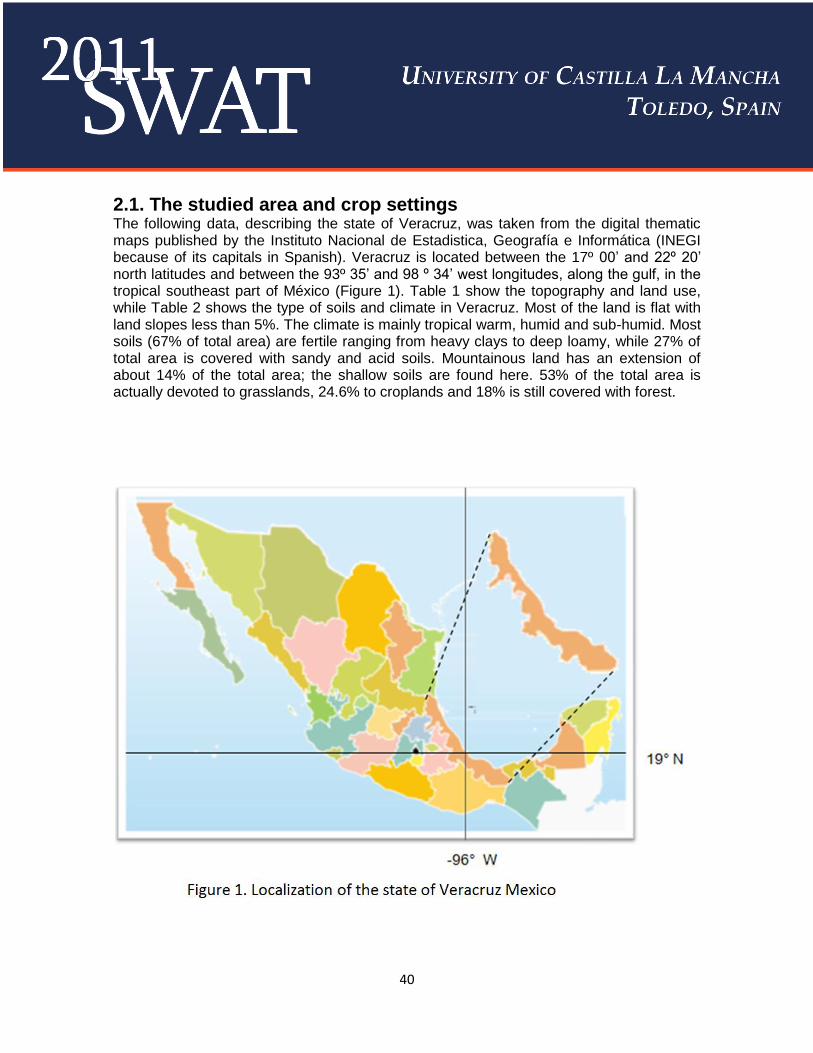
The following data, describing the state of Veracruz, was taken from the digital thematic maps published by the Instituto Nacional de Estadistica, Geografía e Informática (INEGI because of its capitals in Spanish). Veracruz is located between the 17º 00’ and 22º 20’ north latitudes and between the 93º 35’ and 98 º 34’ west longitudes, along the gulf, in the tropical southeast part of México (Figure 1). Table 1 show the topography and land use, while Table 2 shows the type of soils and climate in Veracruz. Most of the land is flat with land slopes less than 5%. The climate is mainly tropical warm, humid and sub-humid. Most soils (67% of total area) are fertile ranging from heavy clays to deep loamy, while 27% of total area is covered with sandy and acid soils. Mountainous land has an extension of about 14% of the total area; the shallow soils are found here. 53% of the total area is actually devoted to grasslands, 24.6% to croplands and 18% is still covered with forest.

41

Table 1. Land slope, and land use in Veracruz, México. Total area: 7.18 million hectares.

Land slope category (%)

% of area Land use category % of area

0 – 5 70 Forest 18.0 5 -15 16 Grassland 53.0 15-30 8 Agricultural 24.6 >30 6 Water bodies and urban 3.6 Total 100 Total 100

Table 2. Climate (Köppen classification) and soil types (FAO soil classification) in Veracruz, México. Total area: 7.18 million hectares.

Type of Climate % of area

Type of soil % of area

Warm, humid: Am1 38 Heavy Clayey (VR, GL)2

34

Warm, sub-humid: Aw 48 Medium Loamy (PH, FL, KS, CM, LV, O)

33

Semi-warm, humid and sub-humid: (A)C(m) and (A)C(w)

7 Light Sandy (RG, AR, CL, SC)

12

Temperate, humid and sub-humid: C(m) and C(w)

6 Acid (AC, AN, NT, PL)

15

Temperate, semi-arid: Bs 1 Shallow (LP)

6

Total 100 Total 100 1Köppen climate classification keys.

2 FAO soil classification Keys.

In México, sugar cane is cropped mainly for the sugar market; production of bioethanol from sugar cane is incipient. Table 3 shows the general statistics of the sugar cane crop in México and Veracruz. Table 3. Average (1997-2007) planted and harvested area (X1000 has) and yield (t ha-1) of sugar cane (fresh stem) in México and Veracruz (SIAP, 2011).

Sugar cane item In México In Veracruz

Planted area (has) 689 253

Harvested area (has) 645 248

Cane (fresh stem) yield (t ha-1) 73.4 72.2

Sugar yield (kg t-1 of fresh stem) 112 112

2.2. SWAT modeling procedure

Simulation and mapping of sugar cane biomass yield was carried out step by step as recommended in the various SWAT manuals and software. The entire area of the state of Veracruz was considered as the basin.

42

2.2.1. Watershed delineation

Watershed delineation was done from a Digital Elevation Model (DEM) with pixel size of 90x90 meters acquired from INEGI, from a mask larger than the state of Veracruz to assure proper shape clip. To increase the flow accuracy in the basin, a river mask was added to the process. The flow direction and accumulation was carried out based on DEM. The stream network was created using the minimum mapping area. Watershed was delineated by selecting all the outlets available; and the sub-basins parameters were calculated with the skip longest flow path calculation on. For the entire area of Veracruz 90 sub-basins were created.

2.2.2. Hydrological Response Units Analysis

The Hydrological Response Units (HRU) were defined from four slope categories map (0-5, 5-15, 15-30 and >30%), 46 soil sub-units (FAO soil classification) and one land use maps; assuming the entire state of Veracruz was cropped to sugar cane. The slope categories were worked out from the DEM, while the soil and land use maps (Scale 1:250,000) were obtained from INEGI. The above process resulted in 6,204 HRU’s.

2.2.3. Database Inputs 2.2.3.1. Soils The typical soil profile for each of the 46 soils was characterized from 829 soil description data sets presented by INEGI along with the digital soil maps. Soil data not given by INEGI was obtained and/or estimated from various sources. The soil profile of an Acrisol humico (ACh) is presented as example in Table 4. Table 4. Characteristics of typical Acrisol humico soil profile.

Horizon Depth (mm)

Clay (%)

Silt (%)

Sand (%)

pH O.C. (%)

albedo K (mmhr-1)

AWC

BD (g cm-3)

A 157 28 27 45 4.80 3.55 0.05 3.7 0.12 1.37 B1 202 39 24 37 4.75 1.58 0.11 2.0 0.12 1.30 B2t 856 44 22 34 4.79 0.66 0.18 1.7 0.12 1.28

O.C.: Organic carbon, K: Saturated hydraulic conductivity, AWC: Available Water Capacity, BD: Bulk density. 2.2.3.2. Land cover/plant grow The sugar cane physiological parameters fed to the model are presented in the Table 5 and were derived from Inman-Bamber, (2004) and local expert opinion. Other parameters were left to be assigned by SWAT. Table 5. Sugar cane physiological parameters fed to SWAT.

Species RUE (Kgha-1/Mjm-2)

2nd point RUE

LAI HI Canopy Height

(m)

Root depth (m)

Optimum temp. ⁰C

Base temp ⁰C

Sugar cane

35 42 8 0.7 3.0 2.0 25 11

43

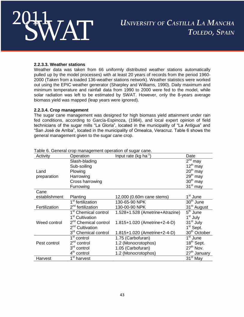
2.2.3.3. Weather stations Weather data was taken from 66 uniformly distributed weather stations automatically pulled up by the model processes) with at least 20 years of records from the period 1960-2000 (Taken from a loaded 136-weather stations network). Weather statistics were worked out using the EPIC weather generator (Sharpley and Williams, 1990). Daily maximum and minimum temperature and rainfall data from 1990 to 2000 were fed to the model, while solar radiation was left to be estimated by SWAT. However, only the 8-years average biomass yield was mapped (leap years were ignored). 2.2.3.4. Crop management The sugar cane management was designed for high biomass yield attainment under rain fed conditions, according to García-Espinoza, (1984), and local expert opinion of field technicians of the sugar mills “La Gloria”, located in the municipality of “La Antigua” and “San José de Arriba”, located in the municipality of Omealca, Veracruz. Table 6 shows the general management given to the sugar cane crop. Table 6. General crop management operation of sugar cane.

Activity Operation Input rate (kg ha-1) Date

Land preparation

Slash-blading 2nd may Sub-soiling 12th may Plowing 20th may Harrowing 29th may Cross harrowing 30th may Furrowing 31st may

Cane establishment

Planting

12,000 (0.60m cane stems)

1st June

Fertilization

1st fertilization 130-65-90 NPK 30th June 2nd fertilization 130-00-90 NPK 31st August

Weed control

1st Chemical control 1.528+1.528 (Ametrine+Atrazine) 5th June 1st Cultivation 1st July 2nd Chemical control 1.815+1.020 (Ametrine+2-4-D) 31st July 2nd Cultivation 1st Sept. 3rd Chemical control 1.815+1.020 (Ametrine+2-4-D) 30th October

Pest control

1st control 1.75 (Carbofuran) 1st June 2nd control 1.2 (Monocrotophos) 18th Sept. 3rd control 1.05 (Carbofuran) 27th Nov. 4th control 1.2 (Monocrotophos) 27th January

Harvest 1st harvest 31st May

44

2.3. Theoretical Bioethanol Calculation Procedure

The theoretical bioethanol yield was calculated for every HRU as the sum of bioethanol from sugar (sucrose), approximately 40% of total, plus the bioethanol from the sugars contained in the cellulose and hemicellulose of tops (crop residue) and bagasse, Approximately 60% of total. Theoretical Bioethanol from sucrose was calculated as the product of fresh stem yield times the rate of theoretical bioethanol production per unit of fresh cane, which was assumed to be 65 L t-1 (Martínez-Jiménez, 2005). The dry biomass yield reported by SWAT was expressed as fresh cane yield by assuming 60% of moisture content (Goldemberg and Guardabassi, 2010). The theoretical bioethanol from tops and bagasse was calculated by multiplying their simulated amount of dry biomass, times the rate of theoretical bioethanol production per unit of biomass. The dry biomass of tops (crop residues) was estimated as recommended by Johnson et al., (2006) from the dry biomass weight reported by SWAT and a harvest index of 0.7. The dry biomass of bagasse was estimated by assuming that 30% of the fresh cane yield was bagasse with a moisture content of 50% after milling, Reyes-Montiel et al., (2005). The rate of bioethanol production from tops and bagasse was calculated with the Theoretical Ethanol Yield Calculator of the Biomass Program of the Department of Energy of the United States of America (http://www1.eere.energy.gov/biomass/ethanol_yield_calculator.html). Table 7 shows the average (six samples) chemical composition of cane bagasse taken from the above electronic page. The fraction of sugars of six and five carbons were input to the model to calculate both; top and bagasse theoretical ethanol yield. Results show volumes of theoretical bioethanol of 269 and 158 L t-1 from sugars of five and six carbons, respectively, giving a total volume of 427 L t-1 of dry tops and bagasse biomass. Table 7. Average chemical composition of sugar cane dry bagasse biomass.

Item

Cellular components (%) of dry matter

Dry matter Sugars (%)

6-carbons 5-carbons

Cellulose Hemicellulose Lignin Gluc Gal Man Xyl Arab

Chemical composition

40.23

24.38

23.56

40.23

0.50

0.33

21.87

1.68

Gluc: Glucan, Gal: Galactan, Man: Mannan, Xyl: Xylan, Arab: Arabinan

45

2.4. Biomass and theoretical bioethanol yield mapping

Fresh cane yield was mapped, then the obtained map was overlaid by a four categories (agricultural, grassland, forest and water bodies and urban) land use map. This operation was done in order to identify and quantify the area every biomass yield range occupies on every actual land use categories. Theoretical bioethanol from sugars was summed to theoretical bioethanol from tops and bagasse to give total theoretical bioethanol yield, which was mapped. From the above maps, compacted areas with high biomass production potential were pin-pointed and bio-refinery capacity was estimated. The areas exceeding 1,200 masl were discarded from the biomass yield map and area quantifications, as it was considered it is the threshold height above sea level for sugar cane growth (see Table 8).

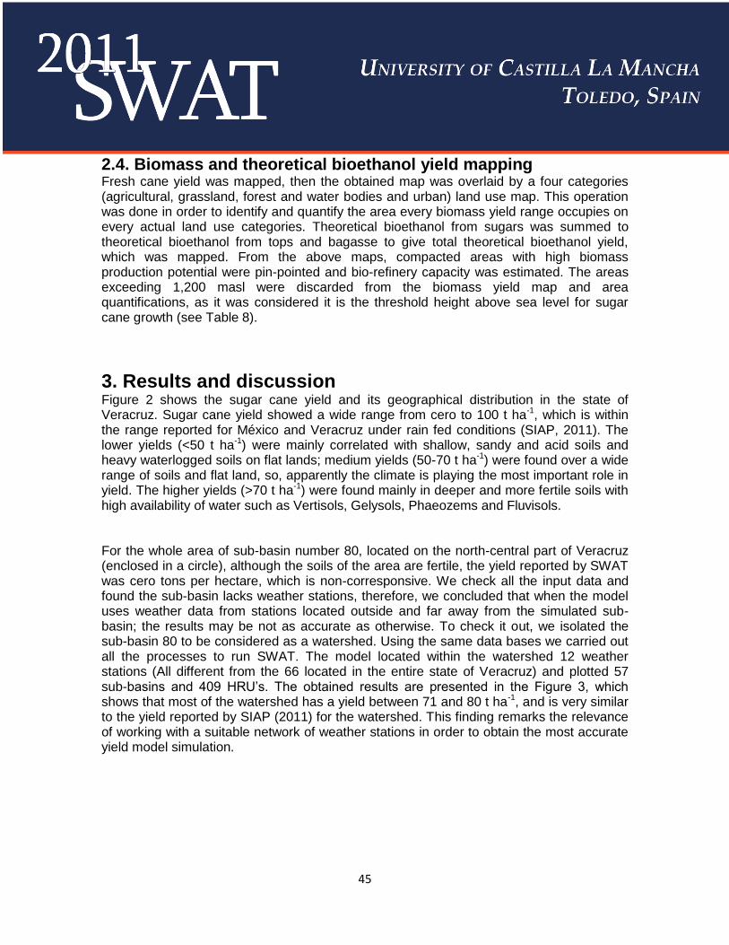
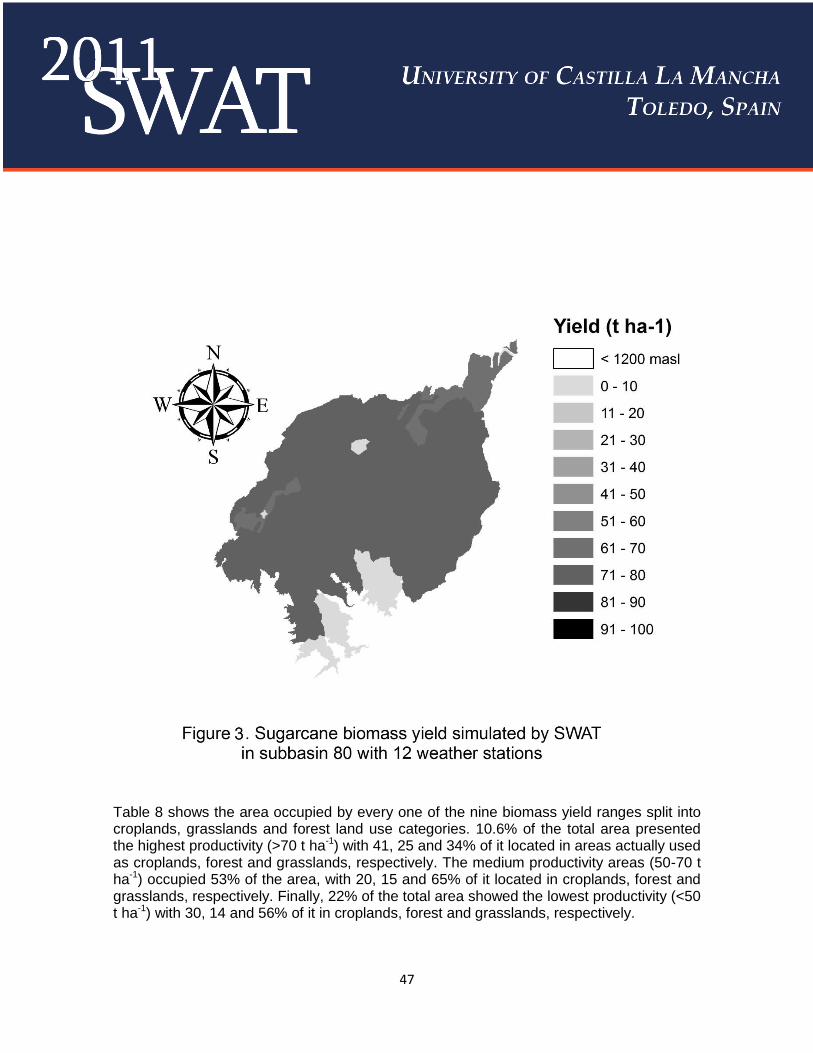
3. Results and discussion Figure 2 shows the sugar cane yield and its geographical distribution in the state of Veracruz. Sugar cane yield showed a wide range from cero to 100 t ha-1, which is within the range reported for México and Veracruz under rain fed conditions (SIAP, 2011). The lower yields (<50 t ha-1) were mainly correlated with shallow, sandy and acid soils and heavy waterlogged soils on flat lands; medium yields (50-70 t ha-1) were found over a wide range of soils and flat land, so, apparently the climate is playing the most important role in yield. The higher yields (>70 t ha-1) were found mainly in deeper and more fertile soils with high availability of water such as Vertisols, Gelysols, Phaeozems and Fluvisols. For the whole area of sub-basin number 80, located on the north-central part of Veracruz (enclosed in a circle), although the soils of the area are fertile, the yield reported by SWAT was cero tons per hectare, which is non-corresponsive. We check all the input data and found the sub-basin lacks weather stations, therefore, we concluded that when the model uses weather data from stations located outside and far away from the simulated sub-basin; the results may be not as accurate as otherwise. To check it out, we isolated the sub-basin 80 to be considered as a watershed. Using the same data bases we carried out all the processes to run SWAT. The model located within the watershed 12 weather stations (All different from the 66 located in the entire state of Veracruz) and plotted 57 sub-basins and 409 HRU’s. The obtained results are presented in the Figure 3, which shows that most of the watershed has a yield between 71 and 80 t ha-1, and is very similar to the yield reported by SIAP (2011) for the watershed. This finding remarks the relevance of working with a suitable network of weather stations in order to obtain the most accurate yield model simulation.

46

At the moment it was not possible to carry out the formal validation of results by plotting simulated versus measured yield, however, from local expert opinion consultation, it may be said that SWAT simulated with reasonable accuracy the sugar cane yield and its spatial distribution in the state of Veracruz, México.

47

Table 8 shows the area occupied by every one of the nine biomass yield ranges split into croplands, grasslands and forest land use categories. 10.6% of the total area presented the highest productivity (>70 t ha-1) with 41, 25 and 34% of it located in areas actually used as croplands, forest and grasslands, respectively. The medium productivity areas (50-70 t ha-1) occupied 53% of the area, with 20, 15 and 65% of it located in croplands, forest and grasslands, respectively. Finally, 22% of the total area showed the lowest productivity (<50 t ha-1) with 30, 14 and 56% of it in croplands, forest and grasslands, respectively.

48

Table 8. Occupied area (X1000 has) by every biomass yield range of king-grass on every

actual land use categories. Biomass

Yield Range t ha

-1

Total

(%) Cropland Forest Grasslands Water Bodies and Urban

Discarded Area *

0-10 237 3.3 106 7 124 0 0

10-20 88 1.2 32 0 56 0 0

20-30 59 0.8 41 8 10 0 0

30-40 376 5.2 142 50 184 0 0

40-50 834 11.7 152 165 517 0 0

50-60 2,503 34.8 496 421 1,585 0 0

60-70 1,281 17.9 245 153 883 0 0

70-80 475 6.6 198 122 155 0 0

80-90 80 1.1 45 9 25 0 0

90-100 218 3.0 73 59 85

Subtotal 6,151 85.6 1,531 995 3,626 0 0

Other 1,036 14.4 0 0 0 247 789

Total

7,187

100

1,531

(21.2%) 995

(14%) 3,626

(50.4%) 247

(3.4%) 789

(11%)

*Discarded area because of exceeding the sugar cane threshold land height above sea level.

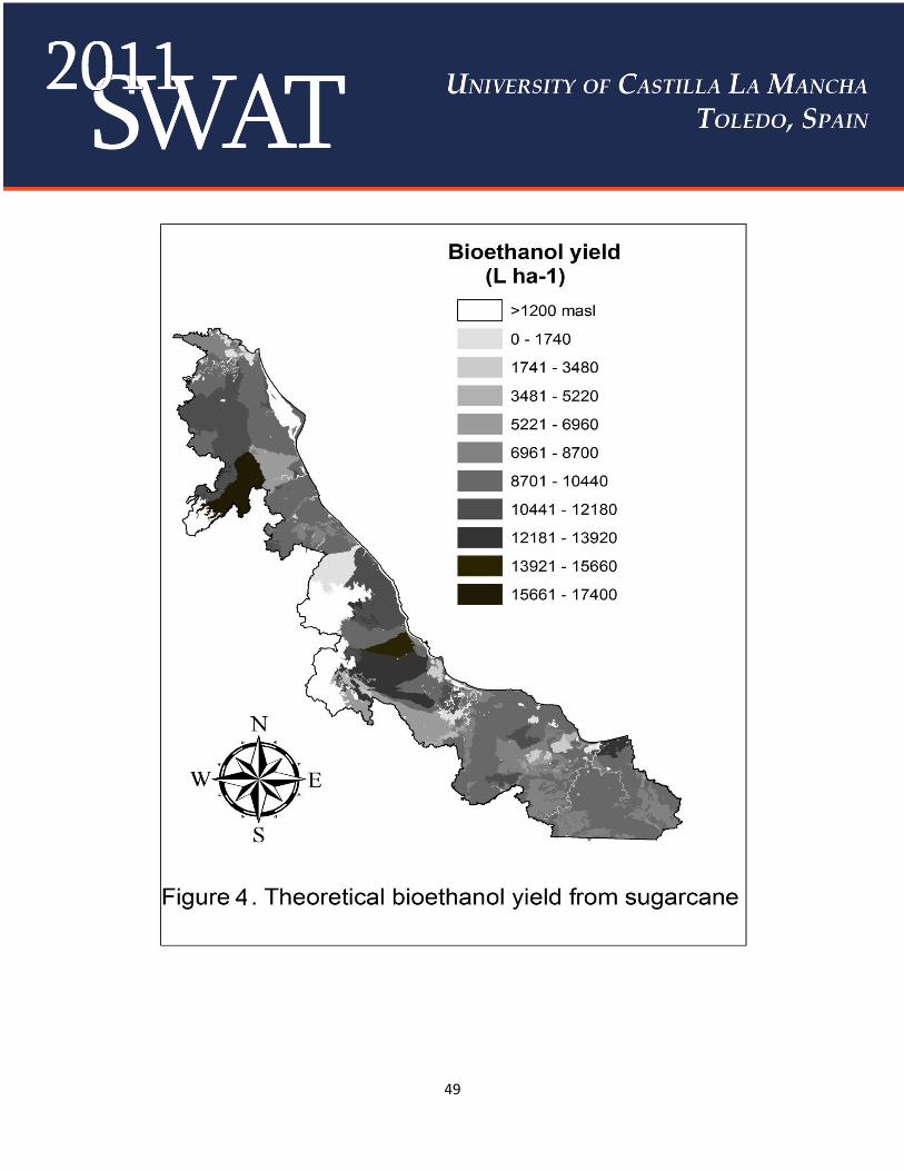
Figure 4 shows the amount and spatial distribution of the total theoretical bioethanol yield. As it was expected, it follows the same pattern as that of biomass yield. For every range, about 40 and 60% of the total bioethanol corresponds to bioethanol from sugars and biomass, respectively. The theoretical volume of bioethanol obtained with the lower and medium ranges (<8,700 and 8,701-12,180 L ha-1) corresponds to the usually reported values for bioethanol from sugar (IICA, 2007; Goldemberg and Guardabassi, 2010; De Vries et al., 2010) and bioethanol from cellulose of crop residues and grasses (Adler et al., 2006; Stork et al., 2009). For the high range (>12,180 L ha-1), the total theoretical bioethanol yield is similar to that of grasses with high biomass yield. In order to obtain relatively and comparable large amounts of bioethanol, it is necessary to consider both ethanol from sugars and ethanol from cellulose and hemicellulose of sugar cane crop residues and bagasse.

49

50

4. Conclusions The biomass and theoretical bioethanol yield of sugar cane from sugars and biomass was simulated and mapped with reasonable accuracy by the SWAT model in the entire state of Veracruz, México; this and related data may assist decision makers in planning bioenergy projects. The SWAT model is a useful tool for planning bioenergy projects and sustainable rural development in tropical watersheds.

Acknowledgements This research was founded by the Mexican Consejo Nacional de Ciencia y Tecnología (CONACYT) and the Consejo Veracruzano de Investigación Científica y Desarrollo Tecnológico (COVEICYDET) through the project VER-2009-C03-128049.

References Adler, P.R., M.A. Sanderson, A.A. Boateng, P.J. Weimer, A.J.G. Jung. 2006. Biomass yield and biofuel quality of switchgrass harvested in fall or spring. Agronomy Journal 98: 1518-1525. Carvalho-Junior, A.M., J. C. Maciel-Ramundo, C. E. de Siqueira-Cavalcanti, P. de S. Faveret-Filho, N.I. Pfefer, S. E. Silveira-da Rosa, A.Y. Milane. 2008. Bioetanol de cana-de-açúcar : Energia para o desenvolvimento sustentável. Organização BNDES e CGEE. – Rio de Janeiro: BNDES. Rio de Janeiro, Brasil. 316p. De Vries, S.C., G.W.J. Van de Ven, M.K. Van Iterrsum, K.E. Giller. 2010. Resource use efficiency and environmental performance of nine major biofuel crops, processed by first generation conversion techniques. Biomass and Bioenergy 34:588-601. Diario Oficial de la Federación (DOF) Secretaría de Energía (SENER). 2009. Reglamento de la Ley de Promoción y Desarrollo de los Bioenergéticos. 19p. Available at: www.diputados.gob.mx/LeyesBiblio/regley/Reg_LPDB.pdf. Accessed on 23th March 2010.

FAO 2008. The Sate of Food and Agriculture: Biofuels: prospects, risks and opportunities. 129p. García-Espinoza, A. 1984. Manual de campo en caña de azúcar. Instituto para el Mejoramiento de la Producción de Azúcar en México. Serie Divulgación Técnica IMPA. 224p. Goldemberg, J., P. Guardabassi, 2010. The potential for first-generation ethanol production from sugar cane. Biofuels, Bioprod. Bioref. 4: 17-24.

51

Inman-Bamber, N. G., 2004. Review of knowledge of sugar cane physiology and climate-crop-soil interaction. Sugar Research and Development Corporation. Australian Government. Final Report No. CSE-006. 77p. Instituto Interamericano de Cooperación para la Agricultura (IICA) 2007. Atlas de la Bioenergía y los Biocombustibles en las Américas. I. Etanol. IICA, San José, Costa Rica. 181p. Johnson, J.M.F., R.R. Allmaras, D.C. Reicosky. 2006. Estimating Source Carbon from Crop Residues, Roots and Rhizodeposits Using the National Grain-Yield Database. Agron. J. 98:622-636.

Liska, A. J., K. G. Cassman. 2008. Towards standardization of Life-Cycle metrics for biofuels: Greenhouse emissions mitigation and net energy yield. Journal of Biobased Materials and Bioenergy. Vol 2. 187-203 Martínez-Jiménez, A. 2005. Uso y beneficio de los biocombustibles. En: Foro: Calidad del aire en el Distrito Federal y Cambio Climático. Secretaría del Medio Ambiente, México. Mayo del 2005. 23p. Menichetti, E., M. Otto. 2009. Energy balance & greenhouse gas emissions of biofuels from a life cycle perspective. In: R. W. Howarth and S. Bringezu (eds) Biofuels: Environmental consequences and interactions with changing land use. Proceedings of the scientific committee on problems of the environment (SCOPE) international biofuels project rapid assessment. 22-25 september 2008, Gummerbach, Germany. Cornell University, Ithaca, NY, USA. p81-109. Neitsch, S.L., J.G. Arnold, J.R. Kiniry, J.R. Williams. 2005. Soil and Water Assessment Tool. Theoretical Documentation, Version 2005. Grassland, Soil and Water Research Laboratory-Agricultural Research Service. Blackland Research Center-Texas Agricultural Experiment Station. Temple, Texas, USA. 476p. Reyes-Montiel, J.R., R.P. Bermúdez, J. B. Mena. 2005. Uso de la biomasa cañera como alternativa para el incremento de la eficiencia energética y la reducción de la contaminación ambiental. Documento interno de trabajo. Centro de Estudios de Termoenergética Azucarera, Universidad Central de las Villas, Santa Clara, Cuba. 9p. Secretaría de Agricultura, Ganadería, Desarrollo Rural, Pesca y Alimentación (SAGARPA). 2007. Programa de producción sustentable de insumos para bioenergéticos y de desarrollo científico y tecnológico. Gobierno Federal, México. 42p. Available at: www.sagarpa.gob.mx/agricultura/.../PROINBIOS_20091013.pdf. Accessed on 9th March 2010. Secretaría de Energía (SENER). 2007. Programa de introducción de bioenergéticos. Gobierno Federal, México. 32p. Available at: www.energia.gob.mx/res/0/Prog%20Introd%20Bioen.pdf accessed on16th March 2010.

52

Stork, J., M. Montross, R. Smith, L. Schwer, W. Chen, M. Reynolds, T. Phillips, T. Coolong, S. Debolt. 2009. Regional examination show potential for native feedstock options for cellulosic biofuel production. GCB Bioenergy 1: 230.239. United States of America. Department of Energy. Biomass Program. Theoretical Ethanol Yield Calculator. Available at: http://www1.eere.energy.gov/biomass/ethanol_yield_calculator.html Accessed on 8th April 2011. Servicio de Información Agroalimentaria y Pesquera (SIAP) 2011. Available at: http://w4.siap.gob.mx/sispro/portales/agricolas/cania/descripcion.pdf Accessed on 27th January 2011. Sharpley, A.N., J.R. Williams. 1990. EPIC-Erosion/Productivity Impact Calculator: 1. Model documentation. U. S. Department of Agriculture. Technical bulletin No. 1768. 235p.