mapping open space in an old-growth, secondary-growth, and selectively-logged tropical rainforest...

IEEE JOURNAL OF SELECTED TOPICS IN APPLIED EARTH OBSERVATIONS AND REMOTE SENSING, VOL. 6, NO. 6, DECEMBER 2013 2453

Mapping Open Space in an Old-Growth,Secondary-Growth, and Selectively-Logged Tropical

Rainforest Using Discrete Return LIDARJinha Jung, Burak K. Pekin, and Bryan C. Pijanowski

Abstract—Light detection and ranging (LIDAR) is a valuabletool for mapping vegetation structure in dense forests. Althoughseveral LIDAR-derived metrics have been proposed for charac-terizing vertical forest structure in previous studies, none of thesemetrics explicitly measure open space, or vertical gaps, under aforest canopy. We develop new LIDAR metrics that characterizevertical gaps within a forest for use in forestry and forest man-agement applications. The proposed metrics are extracted fromdiscrete return LIDAR data acquired over the La Selva BiologicalStation, Costa Rica across three different forest management types(old-growth, secondary-growth, and selectively-logged). A com-parison to common LIDARmetrics of vertical vegetation structurerevealed that our new metrics provide unique information aboutthe structure of the forest canopy. Maps showing the distributionof vertical gap and complex canopy patches identified from ourLIDAR metrics demonstrate that the pattern of open space intropical rain forests is linked to forest management strategies.

Index Terms—Feature extraction, light detection and ranging(LIDAR), vegetation structure characterization, vertical canopygaps.

I. INTRODUCTION

U NDERSTANDING the size distribution of open space,i.e., gaps, in forests is of great importance for forestry and

ecological applications. The location, size, and number of forestgaps allow us to assess vegetation succession dynamics [12],[25] and changes in the habitat of various faunal species [2],[41]. Canopy gaps have commonly been identified and mappedat the plot level through field measurements within a subsampleof the forest, which are used to infer larger scale gap distribu-tions in the forest. Several studies [37], [42] investigated groundsurvey approaches to map canopy gaps. However, Kellner et al.[20] indicated that sample plot-based approaches to mappinggap distribution often underestimate gap sizes and sometimesmiss larger gaps because larger gaps are rare, particularly withinold-growth forests.

Manuscript received April 30, 2012; revised August 13, 2012 and December07, 2012; accepted March 03, 2013. Date of publication April 04, 2013; date ofcurrent version November 21, 2013. This work was supported by the NationalScience Foundation and the U.S. Forest Service under the ULTRA-Ex Programunder Grant 0948484.J. Jung is with the Institute for Environmental Science and Policy, University

of Illinois at Chicago, Chicago, IL 60612 USA (e-mail: [email protected]).B. K. Pekin was with the Forestry and Natural Resources Department, Purdue

University, and is now with the San Diego Zoo Institute for Conservation Re-search, Escondido, CA 92027 USA (e-mail: [email protected]).B. C. Pijanowski is with the Forestry and Natural Resources Department,

Purdue University, West Lafayette, IN 47907 USA (e-mail: [email protected]).Color versions of one or more of the figures in this paper are available online

at http://ieeexplore.ieee.org.Digital Object Identifier 10.1109/JSTARS.2013.2253306

In order to overcome the limitation of the field measurementbased approach, remote sensing techniques have been widelyemployed to map canopy gap distribution. The most popular re-mote sensing data that are utilized to map forest gaps are thosederived from aerial photography [16], [19], [29], [38] and space-borne multispectral imagery [5], [9], [10], [17]. In addition tooptical imagery data, several researchers also investigated uti-lization of a ground based synthetic aperture radar (SAR) [1]and a multifrequency SAR data [14] to characterize complexvegetation structure in tropical rainforest environments. Due toextreme complexity of vegetation structure in tropical rainforestenvironments, Pouteau and Stoll [34] also explored developinga new support vector machine (SVM) based selective data fu-sion algorithm for mapping land cover in tropical rainforest.Recent advances in remote sensing technologies have further

made it possible to capture vertical structural information ofcanopy through light detection and ranging (LIDAR). LIDARis an active remote sensing technology which acquires rangemeasurements, which are then converted into 3-D coordinates ofthe Earth’s surface [22]. The range measurements are obtainedby measuring the outgoing and return flight time of the laserpulses. The time measurements are combined with the location,obtained from global positioning system (GPS), and the attitude,obtained from an inertial measurement unit (IMU), at the timeof the laser shot. One of the advantages of LIDAR technologyis its ability to characterize the three dimensional vertical struc-ture of canopy, which provides a means to assess phenomenathat are occurring in areas that are covered with dense vegeta-tion or have a closed canopy, such as tropical rain forests.A gap is generally defined as a hole in the forest that expands

through all vertical levels down to an average height of 2 mabove the ground [6]. Understanding spatial distribution of gapsand their impact on the dynamics of forest ecosystems has beenof great importance. Researchers have assessed the impact ofcanopy gaps on various forest functions such as lighting con-dition in lower canopy [7], seed dispersal and seedling estab-lishment [12], and canopy composition changes [21]. Severalstudies have also investigated the utilization of LIDAR data formapping canopy gaps in various environments [20], [31], [42].In these studies, canopy gaps were identified based on the tra-ditional definition of forest gap given by Brokaw [6], whichis created from a canopy height model (CHM) derived fromLIDAR data. However, these studies did not incorporate in-formation about the vertical structure of the forest, other thancanopy height, into their forest gap assessment.

1939-1404 © 2013 IEEE

2454 IEEE JOURNAL OF SELECTED TOPICS IN APPLIED EARTH OBSERVATIONS AND REMOTE SENSING, VOL. 6, NO. 6, DECEMBER 2013

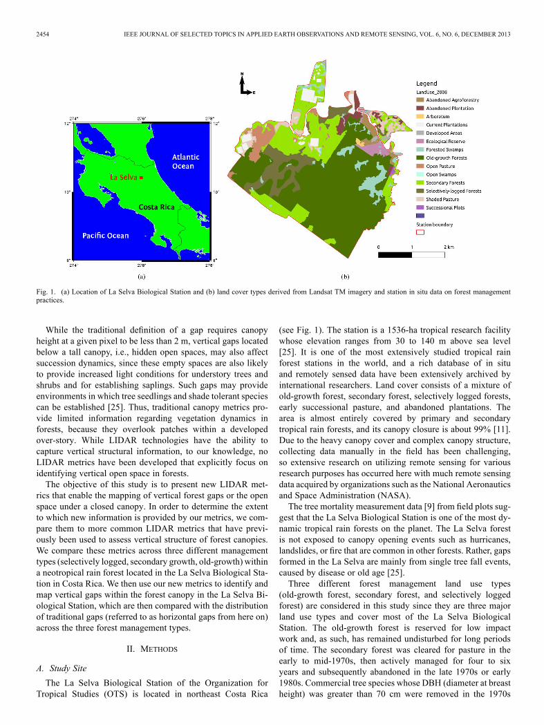
Fig. 1. (a) Location of La Selva Biological Station and (b) land cover types derived from Landsat TM imagery and station in situ data on forest managementpractices.

While the traditional definition of a gap requires canopyheight at a given pixel to be less than 2 m, vertical gaps locatedbelow a tall canopy, i.e., hidden open spaces, may also affectsuccession dynamics, since these empty spaces are also likelyto provide increased light conditions for understory trees andshrubs and for establishing saplings. Such gaps may provideenvironments in which tree seedlings and shade tolerant speciescan be established [25]. Thus, traditional canopy metrics pro-vide limited information regarding vegetation dynamics inforests, because they overlook patches within a developedover-story. While LIDAR technologies have the ability tocapture vertical structural information, to our knowledge, noLIDAR metrics have been developed that explicitly focus onidentifying vertical open space in forests.The objective of this study is to present new LIDAR met-

rics that enable the mapping of vertical forest gaps or the openspace under a closed canopy. In order to determine the extentto which new information is provided by our metrics, we com-pare them to more common LIDAR metrics that have previ-ously been used to assess vertical structure of forest canopies.We compare these metrics across three different managementtypes (selectively logged, secondary growth, old-growth) withina neotropical rain forest located in the La Selva Biological Sta-tion in Costa Rica. We then use our new metrics to identify andmap vertical gaps within the forest canopy in the La Selva Bi-ological Station, which are then compared with the distributionof traditional gaps (referred to as horizontal gaps from here on)across the three forest management types.

II. METHODS

A. Study Site

The La Selva Biological Station of the Organization forTropical Studies (OTS) is located in northeast Costa Rica

(see Fig. 1). The station is a 1536-ha tropical research facilitywhose elevation ranges from 30 to 140 m above sea level[25]. It is one of the most extensively studied tropical rainforest stations in the world, and a rich database of in situand remotely sensed data have been extensively archived byinternational researchers. Land cover consists of a mixture ofold-growth forest, secondary forest, selectively logged forests,early successional pasture, and abandoned plantations. Thearea is almost entirely covered by primary and secondarytropical rain forests, and its canopy closure is about 99% [11].Due to the heavy canopy cover and complex canopy structure,collecting data manually in the field has been challenging,so extensive research on utilizing remote sensing for variousresearch purposes has occurred here with much remote sensingdata acquired by organizations such as the National Aeronauticsand Space Administration (NASA).The tree mortality measurement data [9] from field plots sug-

gest that the La Selva Biological Station is one of the most dy-namic tropical rain forests on the planet. The La Selva forestis not exposed to canopy opening events such as hurricanes,landslides, or fire that are common in other forests. Rather, gapsformed in the La Selva are mainly from single tree fall events,caused by disease or old age [25].Three different forest management land use types

(old-growth forest, secondary forest, and selectively loggedforest) are considered in this study since they are three majorland use types and cover most of the La Selva BiologicalStation. The old-growth forest is reserved for low impactwork and, as such, has remained undisturbed for long periodsof time. The secondary forest was cleared for pasture in theearly to mid-1970s, then actively managed for four to sixyears and subsequently abandoned in the late 1970s or early1980s. Commercial tree species whose DBH (diameter at breastheight) was greater than 70 cm were removed in the 1970s

JUNG et al.: MAPPING OPEN SPACE IN AN OLD-GROWTH, SECONDARY-GROWTH 2455

in the selectively logged forest [8]. These three forest stands,therefore, represent different levels of human disturbance andthus are ideal to determine how forest gaps might vary at a sitewith different forest management regimes. Characteristics ofopen space derived from LIDAR data in these land use typesare compared to see if different forest management land usetypes have impact on spatial distribution of open space in thestudy area.

B. LIDAR Data

An airborne discrete-return LIDAR system with an OptechALTM 3100EA sensor was flown over the study site on 26September 2009 during a 3-h flight period. The ALTM 3100EAsystem operates at 1064 nm and has a 100-kHz maximum pulserate. Its maximum scan angle is 50 degrees, and the sensor candetect up to four returns from each return laser pulse. A returnintensity value was digitized with a 12 bit dynamic range foreach return. The LIDAR system was flown at an altitude of1,500 m with a scan angle of 20 degrees and a 70kHz pulse repetition rate (PRF), which resulted in an averagepoint density of 3.3 points per square meter.A spatial grid structure with 5 m by 5 m spatial resolution

was created to summarize all returns. We chose the 5 m by 5 mgrid structure because this resolution allows for an acceptablesample size of LIDAR data points. There are 82.5 points

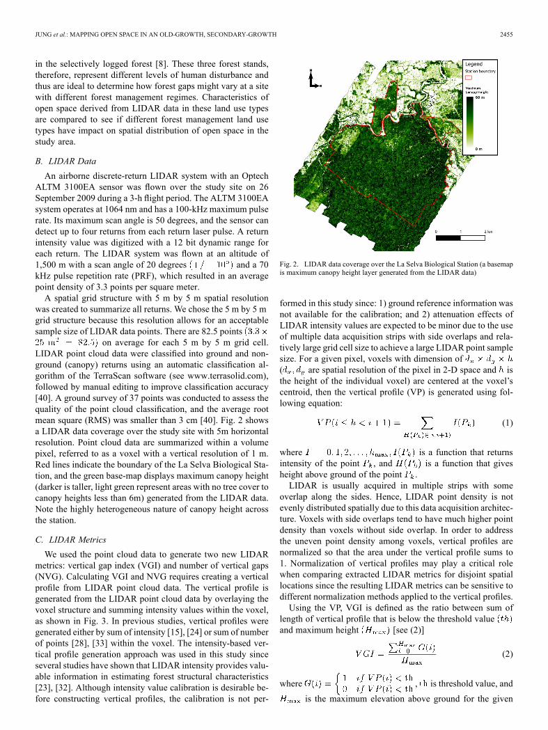
on average for each 5 m by 5 m grid cell.LIDAR point cloud data were classified into ground and non-ground (canopy) returns using an automatic classification al-gorithm of the TerraScan software (see www.terrasolid.com),followed by manual editing to improve classification accuracy[40]. A ground survey of 37 points was conducted to assess thequality of the point cloud classification, and the average rootmean square (RMS) was smaller than 3 cm [40]. Fig. 2 showsa LIDAR data coverage over the study site with 5m horizontalresolution. Point cloud data are summarized within a volumepixel, referred to as a voxel with a vertical resolution of 1 m.Red lines indicate the boundary of the La Selva Biological Sta-tion, and the green base-map displays maximum canopy height(darker is taller, light green represent areas with no tree cover tocanopy heights less than 6m) generated from the LIDAR data.Note the highly heterogeneous nature of canopy height acrossthe station.

C. LIDAR Metrics

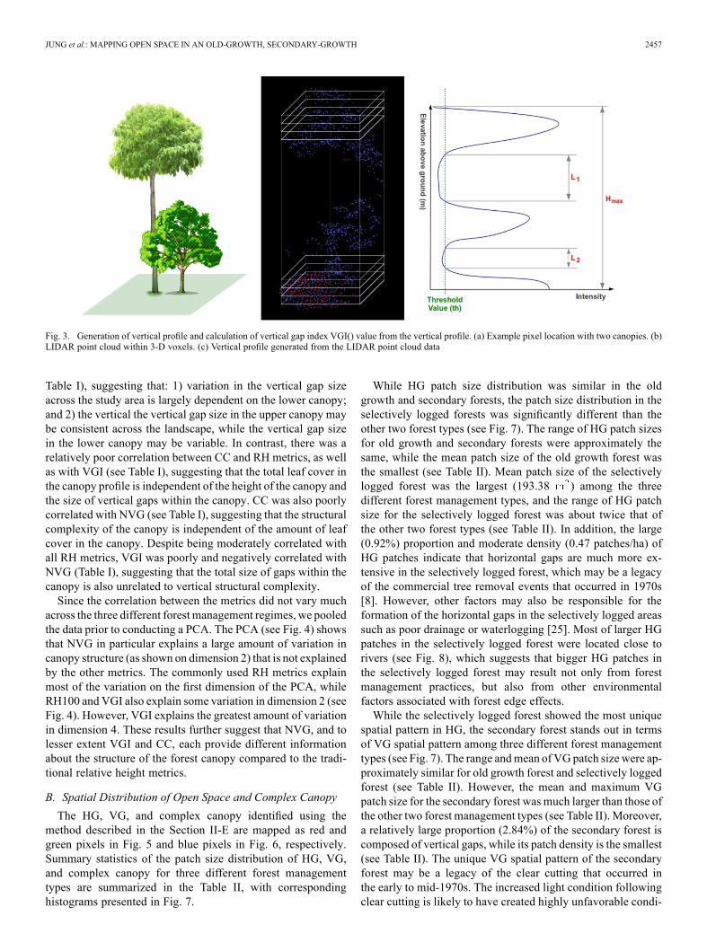
We used the point cloud data to generate two new LIDARmetrics: vertical gap index (VGI) and number of vertical gaps(NVG). Calculating VGI and NVG requires creating a verticalprofile from LIDAR point cloud data. The vertical profile isgenerated from the LIDAR point cloud data by overlaying thevoxel structure and summing intensity values within the voxel,as shown in Fig. 3. In previous studies, vertical profiles weregenerated either by sum of intensity [15], [24] or sum of numberof points [28], [33] within the voxel. The intensity-based ver-tical profile generation approach was used in this study sinceseveral studies have shown that LIDAR intensity provides valu-able information in estimating forest structural characteristics[23], [32]. Although intensity value calibration is desirable be-fore constructing vertical profiles, the calibration is not per-

Fig. 2. LIDAR data coverage over the La Selva Biological Station (a basemapis maximum canopy height layer generated from the LIDAR data)

formed in this study since: 1) ground reference information wasnot available for the calibration; and 2) attenuation effects ofLIDAR intensity values are expected to be minor due to the useof multiple data acquisition strips with side overlaps and rela-tively large grid cell size to achieve a large LIDAR point samplesize. For a given pixel, voxels with dimension of( are spatial resolution of the pixel in 2-D space and isthe height of the individual voxel) are centered at the voxel’scentroid, then the vertical profile (VP) is generated using fol-lowing equation:

(1)

where is a function that returnsintensity of the point , and is a function that givesheight above ground of the point .LIDAR is usually acquired in multiple strips with some

overlap along the sides. Hence, LIDAR point density is notevenly distributed spatially due to this data acquisition architec-ture. Voxels with side overlaps tend to have much higher pointdensity than voxels without side overlap. In order to addressthe uneven point density among voxels, vertical profiles arenormalized so that the area under the vertical profile sums to1. Normalization of vertical profiles may play a critical rolewhen comparing extracted LIDAR metrics for disjoint spatiallocations since the resulting LIDAR metrics can be sensitive todifferent normalization methods applied to the vertical profiles.Using the VP, VGI is defined as the ratio between sum of

length of vertical profile that is below the threshold valueand maximum height [see (2)]

(2)

where , is threshold value, and

is the maximum elevation above ground for the given


voxel. For example, VGI for Fig. 3(c) is calculated as. The VGI value ranges between 0 and 1, and greater

VGI indicates a larger portion of vertical open space betweenthe top of the canopy and the ground. Given that the averagepoint density of the LIDAR point cloud data is approximately3.3 , the common 5 m grid structure has approximately82.5 points per pixel to generate the corresponding vertical pro-file. The VGI is then utilized to identify vertical open spacehidden below taller canopies; these interior vertical gaps aretherefore different from the traditional horizontal gaps.In addition to our VGI that quantifies the amount of vertical

open space, another LIDAR metric that focuses on distributionof vertical gaps is also calculated using the VP. The numberof vertical gaps (NVG) is defined as the number of clusters ofvertical gaps whose response in the vertical profile is below athreshold value that is used in the VGI calculation. Forexample, NVG for Fig. 3(c) is calculated as 2. Larger NVGvalues represent a distribution of vertical gaps that is more dis-continuous, hence the vertical structure within this large NVGcanopy is likely to be more complex than one with lower NVGvalue. Although, VGI and NVG can be calculated based onthe approach described above in most situations, some environ-ments may exist where LiDAR signals fail to penetrate throughcanopies and a higher VGI value may be calculated because ofthe nonfull penetration.Common LIDARmetrics (e.g., RH100, RH75, RH50, RH25,

and CC) that have been used for forest structure characterizationin previous studies [3], [4], [13], [27], [28], [30], [39] were alsocalculated. Relative height (RH) metrics were calculated as ver-tical distance from the ground elevation to the specified energypercentile elevation. Canopy cover (CC) was computed as theenergy ratio between the canopy and the ground return.

D. Comparison of LIDAR Metrics

In order to demonstrate the usefulness of our LIDAR metrics(VGI and NVG), we compare them to common LIDAR met-rics (RH100, RH75, RH50, RH25, CC). We show that the ver-tical structure information of the canopy provided fromVGI andNVG metrics is different from the information delivered fromCC and RH metrics by calculating Pearson’s correlations [35]between all metrics across the three different forest managementtypes. A principal components analysis (PCA) [18] is also con-ducted for all metrics using PCA in the ‘FactoMineR’ packageof R [36] to determine whether each metric explains similar ordifferent variation in the forest structure.

E. Spatial Distribution of Horizontal, Vertical Gaps, andComplex Canopy

To evaluate the performance of the newly proposed LIDARmetrics, we also compared the spatial pattern of our verticalgap metrics VGI and NVG to the spatial patterns of traditionalhorizontal gaps (HG).A map of HG was created using a mean canopy height mea-

sured from the LIDAR data. Points classified as ground areused to create a digital terrain model (DTM) by applying anatural nearest neighbor interpolation. The DTM was used tocompute elevation above ground of each point by subtractingthe corresponding DTM value from the elevation of the point.

Mean canopy height is then calculated by averaging the eleva-tion above ground of points that are within the common 5 mgrid structure used in this study. A horizontal gap is identifiedby applying a 2 m threshold to the mean canopy height layer;in other words, a horizontal gap is defined as any voxel whosecanopy height is 2 m or less.A map of VG was generated based on the VGI layer created

from the LIDAR data. Vertical profiles were generated with 1m elevation spacing (5 m by 5 m by 1 m voxels), and the corre-sponding VGI value is then calculated from the vertical profileusing a threshold value of 0.01 (2). Vertical gaps are de-fined as any voxel whose VGI value is greater than 0.85 in thisstudy, which means approximately more than 85% of verticalspace is empty between the canopy top and the ground.Our NVG metric described in Section II-C is also calculated

from the LIDAR data over the common 5 m grid structure toidentify complex canopy along the forests with three differentmanagement approaches. The complex canopy (CC) is definedas any voxel whose NVG value is greater than 7.The threshold values for mapping VG and CC were chosen

based on the distribution of the VGI and NVG in terms of the99th percentile location for demonstration purpose, since we aremapping vertical open space and complex canopy that are dif-ferent from all others; a value of 0.857 represents the 99th per-centile of VGI, while the value 7 is the 99th percentile of NVG.Wewould like to note that the threshold values used in this studyare arbitrary and different threshold values may be applied de-pending on needs and objectives of specific applications.Patch size frequency analysis was performed for the HG, VG,

and complex canopy metrics using FRAGSTATS [26] softwarewith an 8-cell nearest neighbor rule. HG, VG, and complexcanopy metrics were expressed also as densities calculated bydividing the total area of HG, VG, and complex canopy by thetotal area of the three forest management types. Patch densitywas also computed as the ratio between the number of patchesand total area of each forest management type. Summary statis-tics of patch size was reported, and their patch size histogramsplotted to illustrate size distributions in each of the three forestmanagement types.

III. RESULTS AND DISCUSSION

A. Comparison of Vertical Open Space and Common LIDARMetrics

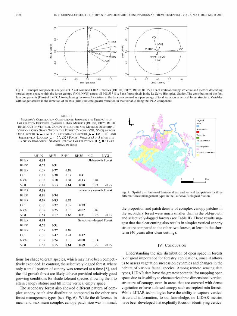
NVG, and to a lesser extent VGI, were weakly correlated withthe common LIDARmetrics across all three forest managementregimes (see Table I). The relative height metrics (RH) gener-ally showed a stronger correlation to each other than to the met-rics describing vertical open space (NVG and VGI; Table I).The exception was a moderate correlation of RH100 with VGIand NVG (see Table I), which suggests that taller canopies arelikely to have a larger gap size and a greater number of verticalgaps. RH75 was highly correlated with RH100 and RH50 (seeTable I). RH25was also highly correlated with RH50 and RH75,and to a lesser extent with RH100 (see Table I), suggesting thatrelative height metrics describe similar structural attributes ofthe canopy. VGI showed a moderate correlation with RH100and RH50 and a stronger correlation with RH50 and RH25 (see


Fig. 3. Generation of vertical profile and calculation of vertical gap index VGI() value from the vertical profile. (a) Example pixel location with two canopies. (b)LIDAR point cloud within 3-D voxels. (c) Vertical profile generated from the LIDAR point cloud data

Table I), suggesting that: 1) variation in the vertical gap sizeacross the study area is largely dependent on the lower canopy;and 2) the vertical the vertical gap size in the upper canopy maybe consistent across the landscape, while the vertical gap sizein the lower canopy may be variable. In contrast, there was arelatively poor correlation between CC and RH metrics, as wellas with VGI (see Table I), suggesting that the total leaf cover inthe canopy profile is independent of the height of the canopy andthe size of vertical gaps within the canopy. CC was also poorlycorrelated with NVG (see Table I), suggesting that the structuralcomplexity of the canopy is independent of the amount of leafcover in the canopy. Despite being moderately correlated withall RH metrics, VGI was poorly and negatively correlated withNVG (Table I), suggesting that the total size of gaps within thecanopy is also unrelated to vertical structural complexity.Since the correlation between the metrics did not vary much

across the three different forest management regimes, we pooledthe data prior to conducting a PCA. The PCA (see Fig. 4) showsthat NVG in particular explains a large amount of variation incanopy structure (as shown on dimension 2) that is not explainedby the other metrics. The commonly used RH metrics explainmost of the variation on the first dimension of the PCA, whileRH100 and VGI also explain some variation in dimension 2 (seeFig. 4). However, VGI explains the greatest amount of variationin dimension 4. These results further suggest that NVG, and tolesser extent VGI and CC, each provide different informationabout the structure of the forest canopy compared to the tradi-tional relative height metrics.

B. Spatial Distribution of Open Space and Complex Canopy

The HG, VG, and complex canopy identified using themethod described in the Section II-E are mapped as red andgreen pixels in Fig. 5 and blue pixels in Fig. 6, respectively.Summary statistics of the patch size distribution of HG, VG,and complex canopy for three different forest managementtypes are summarized in the Table II, with correspondinghistograms presented in Fig. 7.

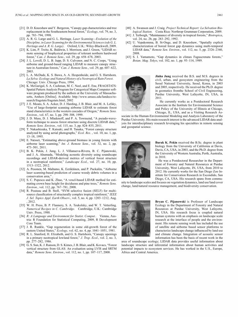
While HG patch size distribution was similar in the oldgrowth and secondary forests, the patch size distribution in theselectively logged forests was significantly different than theother two forest types (see Fig. 7). The range of HG patch sizesfor old growth and secondary forests were approximately thesame, while the mean patch size of the old growth forest wasthe smallest (see Table II). Mean patch size of the selectivelylogged forest was the largest (193.38 ) among the threedifferent forest management types, and the range of HG patchsize for the selectively logged forest was about twice that ofthe other two forest types (see Table II). In addition, the large(0.92%) proportion and moderate density (0.47 patches/ha) ofHG patches indicate that horizontal gaps are much more ex-tensive in the selectively logged forest, which may be a legacyof the commercial tree removal events that occurred in 1970s[8]. However, other factors may also be responsible for theformation of the horizontal gaps in the selectively logged areassuch as poor drainage or waterlogging [25]. Most of larger HGpatches in the selectively logged forest were located close torivers (see Fig. 8), which suggests that bigger HG patches inthe selectively logged forest may result not only from forestmanagement practices, but also from other environmentalfactors associated with forest edge effects.While the selectively logged forest showed the most unique

spatial pattern in HG, the secondary forest stands out in termsof VG spatial pattern among three different forest managementtypes (see Fig. 7). The range andmean ofVG patch size were ap-proximately similar for old growth forest and selectively loggedforest (see Table II). However, the mean and maximum VGpatch size for the secondary forest was much larger than those ofthe other two forest management types (see Table II). Moreover,a relatively large proportion (2.84%) of the secondary forest iscomposed of vertical gaps, while its patch density is the smallest(see Table II). The unique VG spatial pattern of the secondaryforest may be a legacy of the clear cutting that occurred inthe early to mid-1970s. The increased light condition followingclear cutting is likely to have created highly unfavorable condi-


Fig. 4. Principal components analysis (PCA) of common LIDAR metrics (RH100, RH75, RH50, RH25, CC) of vertical canopy structure and metrics describingvertical open space within the forest canopy (VGI, NVG) across all 508 537 (5 x 5 m) forest pixels in the La Selva Biological Station.The contribution of the firstfour components (Dim) of the PCA to explaining the overall variation in the data is expressed as a percentage of total variation in vertical forest structure. Variableswith longer arrows in the direction of an axis (Dim) indicate greater variation in that variable along that PCA component.

TABLE IPEARSON’S CORRELATION COEFFICIENTS SHOWING THE STRENGTH OF

CORRELATION BETWEEN COMMON LIDAR METRICS (RH100, RH75, RH50,RH25, CC) OF VERTICAL CANOPY STRUCTURE AND METRICS DESCRIBINGVERTICAL OPEN SPACE WITHIN THE FOREST CANOPY (VGI, NVG) ACROSSOLD-GROWTH , SECONDARY-GROWTH , ANDSELECTIVELY-LOGGED FOREST VOXELS (5 5 m) IN THELA SELVA BIOLOGICAL STATION. STRONG CORRELATIONS ARE

SHOWN IN BOLD

tions for shade tolerant species, which may have been competi-tively excluded. In contrast, the selectively logged forest, whereonly a small portion of canopy was removed at a time [8], andthe old-growth forest are likely to have provided relatively goodgrowing conditions for shade tolerant species allowing them toattain canopy stature and fill in the vertical empty space.The secondary forest also showed different pattern of com-

plex canopy patch size distribution compared to the other twoforest management types (see Fig. 6). While the difference inmean and maximum complex canopy patch size was minimal,

Fig. 5. Spatial distribution of horizontal gap and vertical gap patches for threedifferent forest management types in the La Selva Biological Station.

the proportion and patch density of complex canopy patches inthe secondary forest were much smaller than in the old-growthand selectively-logged forests (see Table II). These results sug-gest that the clear cutting also results in simpler vertical canopystructure compared to the other two forests, at least in the shortterm (40 years after clear cutting).

IV. CONCLUSION

Understanding the size distribution of open space in forestsis of great importance for forestry applications, since it allowsus to assess vegetation succession dynamics and changes in thehabitat of various faunal species. Among remote sensing datatypes, LIDAR data have the greatest potential for mapping openspace due to its ability to characterize three dimensional verticalstructure of canopy, even in areas that are covered with densevegetation or have a closed canopy such as tropical rain forests.While LIDAR technologies have the ability to capture verticalstructural information, to our knowledge, no LIDAR metricshave been developed that explicitly focus on identifying vertical


Fig. 6. Spatial distribution of complex canopy patches for three different forest management types in the La Selva Biological Station.

TABLE IISUMMARY STATISTICS OF PATCH SIZE DISTRIBUTION OF HORIZONTAL GAP, VERTICAL GAP, AND COMPLEX CANOPY ACROSS OLD-GROWTH FOREST (OGF),SECONDARY FOREST (SF), AND SELECTIVELY-LOGGED FOREST (SLF) IN THE LA SELVA BIOLOGICAL STATION. MINIMUM (MIN), MAXIMUM (MAX), AND

AVERAGE (MEAN) SIZE OF PATCHES IS SHOWN FOR EACH GAP AND FOREST MANAGEMENT TYPE. THE PROPORTION (%) OF AREA THAT IS COMPOSED OF GAPSAND THE NUMBER OF PATCHES RELATIVE TO THE TOTAL AREA (PATCH DENSITY) IN EACH FOREST MANAGEMENT TYPE IS ALSO SHOWN

open space. To deal with this issue, new LIDAR metrics (VGIand NVG) that enable the mapping of vertical gaps or the openspace under a closed canopy are proposed in this study. The newLIDAR metrics are compared to several common LIDAR met-rics (relative height and canopy cover) that have been previouslyused to assess vertical structure of forest canopies. Pearson’scorrelation coefficients and PCA analyses showed that NVG,and to lesser extent VGI, provide different information aboutthe structure of the forest canopy than canopy cover and relativeheight metrics. VGI and NVGwere also used to identify patches

of vertical gaps and complex canopy, the size distribution ofwhichwere determined across three differentmanagement types(selectively logged, secondary growth, old-growth). The spatialdistribution of vertical gaps and complex canopy patches variedacross the forest management types, which has implications forbiodiversity and species habitat management. Thus, studies in-vestigating the relationship between vertical open space andspecies diversity are likely to be highly useful for forest bio-diversity conservation applications. Although little focus wasplaced on methods for vertical profile generation and normal-


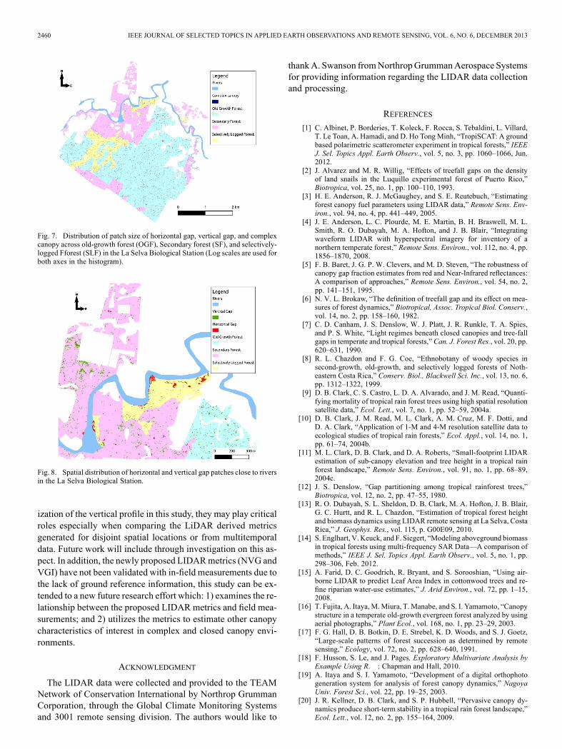
Fig. 7. Distribution of patch size of horizontal gap, vertical gap, and complexcanopy across old-growth forest (OGF), Secondary forest (SF), and selectively-logged Fforest (SLF) in the La Selva Biological Station (Log scales are used forboth axes in the histogram).

Fig. 8. Spatial distribution of horizontal and vertical gap patches close to riversin the La Selva Biological Station.

ization of the vertical profile in this study, they may play criticalroles especially when comparing the LiDAR derived metricsgenerated for disjoint spatial locations or from multitemporaldata. Future work will include through investigation on this as-pect. In addition, the newly proposed LIDARmetrics (NVG andVGI) have not been validated with in-field measurements due tothe lack of ground reference information, this study can be ex-tended to a new future research effort which: 1) examines the re-lationship between the proposed LIDAR metrics and field mea-surements; and 2) utilizes the metrics to estimate other canopycharacteristics of interest in complex and closed canopy envi-ronments.

ACKNOWLEDGMENT

The LIDAR data were collected and provided to the TEAMNetwork of Conservation International by Northrop GrummanCorporation, through the Global Climate Monitoring Systemsand 3001 remote sensing division. The authors would like to

thankA. Swanson fromNorthropGrummanAerospace Systemsfor providing information regarding the LIDAR data collectionand processing.

REFERENCES

[1] C. Albinet, P. Borderies, T. Koleck, F. Rocca, S. Tebaldini, L. Villard,T. Le Toan, A. Hamadi, and D. Ho Tong Minh, “TropiSCAT: A groundbased polarimetric scatterometer experiment in tropical forests,” IEEEJ. Sel. Topics Appl. Earth Observ., vol. 5, no. 3, pp. 1060–1066, Jun.2012.

[2] J. Alvarez and M. R. Willig, “Effects of treefall gaps on the densityof land snails in the Luquillo experimental forest of Puerto Rico,”Biotropica, vol. 25, no. 1, pp. 100–110, 1993.

[3] H. E. Anderson, R. J. McGaughey, and S. E. Reutebuch, “Estimatingforest canopy fuel parameters using LIDAR data,” Remote Sens. Env-iron., vol. 94, no. 4, pp. 441–449, 2005.

[4] J. E. Anderson, L. C. Plourde, M. E. Martin, B. H. Braswell, M. L.Smith, R. O. Dubayah, M. A. Hofton, and J. B. Blair, “Integratingwaveform LIDAR with hyperspectral imagery for inventory of anorthern temperate forest,” Remote Sens. Environ., vol. 112, no. 4, pp.1856–1870, 2008.

[5] F. B. Baret, J. G. P. W. Clevers, and M. D. Steven, “The robustness ofcanopy gap fraction estimates from red and Near-Infrared reflectances:A comparison of approaches,” Remote Sens. Environ., vol. 54, no. 2,pp. 141–151, 1995.

[6] N. V. L. Brokaw, “The definition of treefall gap and its effect on mea-sures of forest dynamics,” Biotropical, Assoc. Tropical Biol. Conserv.,vol. 14, no. 2, pp. 158–160, 1982.

[7] C. D. Canham, J. S. Denslow, W. J. Platt, J. R. Runkle, T. A. Spies,and P. S. White, “Light regimes beneath closed canopies and tree-fallgaps in temperate and tropical forests,” Can. J. Forest Res., vol. 20, pp.620–631, 1990.

[8] R. L. Chazdon and F. G. Coe, “Ethnobotany of woody species insecond-growth, old-growth, and selectively logged forests of Noth-eastern Costa Rica,” Conserv. Biol., Blackwell Sci. Inc., vol. 13, no. 6,pp. 1312–1322, 1999.

[9] D. B. Clark, C. S. Castro, L. D. A. Alvarado, and J. M. Read, “Quanti-fying mortality of tropical rain forest trees using high spatial resolutionsatellite data,” Ecol. Lett., vol. 7, no. 1, pp. 52–59, 2004a.

[10] D. B. Clark, J. M. Read, M. L. Clark, A. M. Cruz, M. F. Dotti, andD. A. Clark, “Application of 1-M and 4-M resolution satellite data toecological studies of tropical rain forests,” Ecol. Appl., vol. 14, no. 1,pp. 61–74, 2004b.

[11] M. L. Clark, D. B. Clark, and D. A. Roberts, “Small-footprint LIDARestimation of sub-canopy elevation and tree height in a tropical rainforest landscape,” Remote Sens. Environ., vol. 91, no. 1, pp. 68–89,2004c.

[12] J. S. Denslow, “Gap partitioning among tropical rainforest trees,”Biotropica, vol. 12, no. 2, pp. 47–55, 1980.

[13] R. O. Dubayah, S. L. Sheldon, D. B. Clark, M. A. Hofton, J. B. Blair,G. C. Hurtt, and R. L. Chazdon, “Estimation of tropical forest heightand biomass dynamics using LIDAR remote sensing at La Selva, CostaRica,” J. Geophys. Res., vol. 115, p. G00E09, 2010.

[14] S. Englhart, V. Keuck, and F. Siegert, “Modeling aboveground biomassin tropical forests using multi-frequency SAR Data—A comparison ofmethods,” IEEE J. Sel. Topics Appl. Earth Observ., vol. 5, no. 1, pp.298–306, Feb. 2012.

[15] A. Farid, D. C. Goodrich, R. Bryant, and S. Sorooshian, “Using air-borne LIDAR to predict Leaf Area Index in cottonwood trees and re-fine riparian water-use estimates,” J. Arid Environ., vol. 72, pp. 1–15,2008.

[16] T. Fujita, A. Itaya, M.Miura, T. Manabe, and S. I. Yamamoto, “Canopystructure in a temperate old-growth evergreen forest analyzed by usingaerial photographs,” Plant Ecol., vol. 168, no. 1, pp. 23–29, 2003.

[17] F. G. Hall, D. B. Botkin, D. E. Strebel, K. D. Woods, and S. J. Goetz,“Large-scale patterns of forest succession as determined by remotesensing,” Ecology, vol. 72, no. 2, pp. 628–640, 1991.

[18] F. Husson, S. Le, and J. Pages, Exploratory Multivariate Analysis byExample Using R. : Chapman and Hall, 2010.

[19] A. Itaya and S. I. Yamamoto, “Development of a digital orthophotogeneration system for analysis of forest canopy dynamics,” NagoyaUniv. Forest Sci., vol. 22, pp. 19–25, 2003.

[20] J. R. Kellner, D. B. Clark, and S. P. Hubbell, “Pervasive canopy dy-namics produce short-term stability in a tropical rain forest landscape,”Ecol. Lett., vol. 12, no. 2, pp. 155–164, 2009.


[21] D. D. Kneeshaw and Y. Bergeron, “Canopy gap characteristics and treereplacement in the Southeastern boreal forest,” Ecology, vol. 79, no. 3,pp. 783–794, 1998.

[22] A. R. G. Large and G. L. Heritage, Laser Scanning—Evolution of theDiscipline, in Laser Scanning for the Environmental Sciences (edsG. L.Heritage and A. R. G. Large). Oxford, U.K.: Wiley-Blackwell, 2009.

[23] K. Lim, P. Treitz, K. Baldwin, I. Morrison, and J. Green, “LIDAR re-mote sensing of biophysical properties of tolerant northern hardwoodforest,” Can. J. Remote Sens., vol. 29, pp. 658–678, 2003.

[24] J. L. Lovell, D. L. B. Jupp, D. S. Culvenor, and N. C. Coops, “Usingairborne and ground-based ranging LIDAR to measure canopy struc-ture in Australian forests,” Can. J. Remote Sens., vol. 29, pp. 607–622,2003.

[25] L. A. McDade, K. S. Bawa, A. A. Hespenheide, and G. S. Hartshorn,La Selva: Ecology and Natural History of a Neotropical Rain Forest.Chicago: Univ. Chicago Press, 1994.

[26] K. McGarigal, S. A. Cushman, M. C. Neel, and E. Ene, FRAGSTATS:Spatial Pattern Analysis Program for Categorical Maps Computer soft-ware program produced by the authors at the University of Massachu-setts, Amhers [Online]. Available: http://www.umass.edu/landeco/re-search/fragstats/fragstats.html, 2002

[27] J. E. Means, S. A. Acker, D. J. Harding, J. B. Blair, and M. A. Lefsky,“Use of large-footprint scanning airborne LIDAR to estimate foreststand characteristics in the western cascades of Oregon,” Remote Sens.Environ., vol. 67, no. 3, pp. 298–308, 1999.

[28] J. D. Muss, D. J. Mladenoff, and P. A. Townsend, “A pseudo-wave-form technique to assess forest structure using discrete LIDAR data,”Remote Sens. Environ., vol. 115, no. 3, pp. 824–835, 2011.

[29] T. Nakashizuka, T. Katsuki, and H. Tanaka, “Forest canopy structureanalyzed by using aerial photographs,” Ecol. Res. , vol. 10, no. 1, pp.13–18, 1995.

[30] E. Næsset, “Estimating above-ground biomass in young forests withairborne laser scanning,” Int. J. Remote Sens., vol. 32, no. 2, pp.473–501, 2011.

[31] B. K. Pekin, J. Jung, L. J. Villanueva-Rivera, B. C. Pijanowski,and J. A. Ahumada, “Modeling acoustic diversity using soundscaperecordings and LIDAR-derived metrics of vertical forest structurein a neotropical rainforest,” Landscape Ecol., vol. 27, no. 10, pp.1513–1522, 2012.

[32] A. Pesonen, M. Maltamo, K. Eerikäinen, and P. Packalèn, “Airbornelaser scanning-based prediction of coarse woody debris volumes in aconservation area,” .

[33] S. C. Popescu and K. Zhao, “A voxel-based LIDAR method for esti-mating crown base height for deciduous and pine trees,” Remote Sens.Environ., vol. 112, pp. 767–781, 2008.

[34] R. Pouteau and B. Stoll, “SVM selective fusion (SELF) for multi-source classification of structurally complex tropical rainforest,” IEEEJ. Sel. Topics Appl. Earth Observ., vol. 5, no. 4, pp. 1203–1212, Aug., 2012.

[35] W. H. Press, B. P. Flannery, S. A. Teukolsky, and W. T. Vetterling,Numerical Recipes in C. Cambridge. Cambridge, U.K.: CambridgeUniv. Press, 1988.

[36] R: A Language and Environment for Statist. Comput.. Vienna, Aus-tria: R Foundation for Statistical Computing, 2009, R DevelopmentCore Team.

[37] J. R. Runkle, “Gap regeneration in some old-growth forest of theeastern United States,” Ecology, vol. 62, no. 4, pp. 1041–1051, 1981.

[38] R. L. Stanford, H. Elizabeth, and G. S. Hartshorn, “Canopy openingsin a primary neotropical lowland forest,” J. Trop. Ecol., vol. 2, no. 3,pp. 277–282, 1986.

[39] G. S. Sun, K. J. Ranson, D. S. Kimes, J. B. Blair, andK.Kovacs, “Forestvertical structure from GLAS: An evaluation using LVIS and SRTMdata,” Remote Sens. Environ., vol. 112, no. 1, pp. 107–117, 2008.

[40] A. Swanson and J. Craig, Project Technical Report: La Selvation Bio-logical Station. Costa Rica: Northrop Grumman Corporation, 2009.

[41] J. Terborgh, “Maintanance of diversity in tropical forests,” Biotropica,vol. 24, no. 2b, pp. 283–292, 1992.

[42] U. Vepakomma, B. St-Onge, and D. Kneeshaw, “Spatially explicitcharacterization of boreal forest gap dynamics using multi-temporalLIDAR data,” Remote Sen. Environ., vol. 112, no. 5, pp. 2326–2340,2008.

[43] S. I. Yamamoto, “Gap dynamics in climax Faguscrenata forests,”Botan. Mag. Tokyo, vol. 102, no. 1, pp. 93–114, 1989.

Jinha Jung received the B.S. and M.S. degrees incivil, urban, and geosystem engineering from theSeoul National University, Seoul, Korea, in 2003and 2005, respectively. He received the Ph.D. degreein geomatics fromthe School of Civil Engineering,Purdue University, West Lafayette, IN, USA, in2011.He currently works as a Postdoctoral Research

Associate in the Institute for Environmental Scienceand Policy of the University of Illinois at Chicago,Chicago, IL, USA, and as a Visiting Research As-

sociate in the Human-Environmental Modeling and Analysis Laboratory of thePurdue University. His main research interest is the advanced LIDAR data anal-ysis for interdisciplinary research leveraging his specialties in remote sensingand geospatial science.

Burak K. Pekin received the B.Sc. degree in plantbiology from the University of California at Davis,Davis, CA, USA, in 2003, and the Ph.D. degree fromthe University of Western Australia, Perth, Australia,in 2010.He was a Postdoctoral Researcher in the Depart-

ment of Forestry and Natural Resources at PurdueUniversity, West Lafayette, IN, USA, from 2010 to2012. He currently works for the San Diego Zoo In-stitute for Conservation Research in Escondido, SanDiego, CA, USA. His research spans from commu-

nity to landscape scales and focuses on vegetation dynamics, land use/land coverchange, land/natural resource management, and biodiversity conservation.

Bryan C. Pijanowski is Professor of LandscapeEcology in the Department of Forestry and NaturalResources at Purdue University, West Lafayette,IN, USA. His research focus is coupled naturalhuman systems with an emphasis on landscape scaleresearch at the interface of people and the environ-ment. His remote sensing work has included the useof satellite and airborne based sensor platforms tocharacterize landscape change influenced by land useand climate change. Integration of acoustic sensorinformation has been the basis of recent work in the

area of soundscape ecology; LIDAR data provides useful information aboutlandscape structure and inferential information about human activities andpotential impacts to ecosystem services. He has worked in the U.S., Europe,Africa and Central America.

mapping open space in an old-growth, secondary-growth, and selectively-logged tropical rainforest...

Documents