This content has been downloaded from IOPscience. Please scroll down to see the full text.

Download details:

IP Address: 129.215.5.251

This content was downloaded on 05/06/2014 at 10:32

Please note that terms and conditions apply.

Mapping multiplicative to additive noise

View the table of contents for this issue, or go to the journal homepage for more

2014 J. Phys. A: Math. Theor. 47 195001

(http://iopscience.iop.org/1751-8121/47/19/195001)

Home Search Collections Journals About Contact us My IOPscience

Journal of Physics A: Mathematical and Theoretical

J. Phys. A: Math. Theor. 47 (2014) 195001 (18pp) doi:10.1088/1751-8113/47/19/195001

Mapping multiplicative to additive noise

Katy J Rubin, Gunnar Pruessner and Grigorios A Pavliotis

Department of Mathematics, Imperial College London, 180 Queen’s Gate,London SW7 2BZ, UK

E-mail: gunnar.pruessner@physics.org

Received 3 January 2014, revised 19 March 2014Accepted for publication 2 April 2014Published 23 April 2014

AbstractThe Langevin formulation of a number of well-known stochastic processesinvolves multiplicative noise. In this work we present a systematic mappingof a process with multiplicative noise to a related process with additive noise,which may often be easier to analyse. The mapping is easily understood inthe example of the branching process. In a second example we study therandom neighbour (or infinite range) contact process which is mapped to anOrnstein–Uhlenbeck process with absorbing wall. The present work might shedsome light on absorbing state phase transitions in general, such as the role ofconditional expectation values and finite size scaling, and elucidate the meaningof the noise amplitude. While we focus on the physical interpretation of themapping, we also provide a mathematical derivation.

Keywords: multiplicative noise, phase transitions, non-equilibriumPACS numbers: 74.40.Gh, 68.35.rh

1. Introduction

In many stochastic processes, activity cannot recover once it has ceased. This feature is atthe centre of absorbing state phase transitions [1] which in turn makes a significant part ofthe wider field of non-equilibrium phase transitions [2]. In an equation of motion of a singledegree of freedom ψ(g) as a function of time g, the feature enters as a multiplicative noise,such as

∂gψ(g) = f (ψ(g)) +√

ψ(g)η(g), (1)

where f (ψ) is a generic function with the property f (0) = 0 and η(g) is a noise process, tobe specified below. Crucially, if ψ vanishes at any time g∗ it will remain 0 for all future times.This is exactly the feature expected in an absorbing state phase transition and, closely related,in Reggeon field theory [1, 3].

In this paper we will consider the case where η(g) represents standard white noise andwe will consider the Ito interpretation of the stochastic term in (1). This equation can be

1751-8113/14/195001+18$33.00 © 2014 IOP Publishing Ltd Printed in the UK 1

J. Phys. A: Math. Theor. 47 (2014) 195001 K J Rubin et al

solved either numerically (or even analytically in special cases), or the corresponding Fokker–Planck equation that governs the evolution of the transition probability density can be studied.In the following, we will trace the origin of the multiplicative noise which will provide analternative formulation of the process with additive noise; as an added benefit, nonlinearitiesmay simplify significantly, making a direct solution of the stochastic differential equation(SDE) more feasible.

It should be emphasized that a SDE of the form (1), which we rewrite here for amultiplicative noise that is an arbitrary function of ψ

dψ(g) = f (ψ(g)) dt +√

σ (ψ(g)) dW (g), (2)

where W (g) denotes standard one-dimensional Brownian motion, does not provide us witha complete description of the dynamics, since noise in this equation (or, equivalently, thestochastic integral when writing it as an integral equation) can be interpreted in differentways, including the well known Ito and Stratonovich interpretations [4]. This is a modellingissue and it has to be addressed separately. The Wong–Zakai theorem [5] suggests that whenthinking of white noise as an idealization of a noise process with a non-zero correlation time,then the noise in (2) should be interpreted in the Stratonovich sense. On the other hand, it isby now well known that for stochastic systems with more than one fast time scale (one beingthe correlation time of the approximation to white noise, the other being, e.g. a timescalemeasuring the inertia of the system), in the limit as these timescales tending to zero, we obtaina SDE that can be of Ito or Stratonovich type, or neither [6, 7]. Making the physically correctchoice of the type of noise in (2) is crucial, since different interpretations of the noise lead toSDEs with qualitatively different features. A standard example is geometric Brownian motion:the long time behaviour of solutions to this equation (for fixed values of the parameters in theSDE) can be different for the Ito and Stratonovich SDEs [8]. In this paper we will choose theIto interpretation of noise. It is well known that it is possible to switch between differentinterpretations of the noise by adding an appropriate drift (which, of course, changes generallythe qualitative properties of solutions to the SDE).

SDEs with multiplicative noise exhibit a very rich dynamical behaviour includingintermittency and noise induced transitions [9]. On the other hand, state-dependent noise leadsto analytical, numerical and even statistical difficulties, i.e. it is more difficult to estimate state-dependent noise from observations as opposed to estimating a constant diffusion coefficient;see, e.g. [10]. It is natural, therefore, to ask whether it is possible to find an appropriatetransformation that maps SDEs with multiplicative noise to SDEs with additive noise. Thisis possible in one dimension: an application of Ito’s formula to the function (assuming, ofcourse, that this function exists)

h(x) =∫ x 1√

σ (ψ)dψ, (3)

enables us to transform (2) into an SDE with additive noise for the new process

z(g) = h(ψ(g)), (4)

see, e.g. [4]. This transformation can also be performed at the level of the correspondingFokker–Planck equation, see e.g. [11]. Such a transformation mapping multiplicative toadditive noise does not generally exist in dimensions greater than one, unless the diffusionmatrix satisfies appropriate compatibility conditions [10].

In this paper, we adopt a different approach: we introduce a new clock, so that, whenmeasuring time with respect to this new time scale, noise becomes additive. Clearly, in orderfor this to be possible, the transformation to the new time must involve the actual solution ofthe SDE. The theoretical basis for this random time change is the Dambis–Dubins–Schwarz

2

J. Phys. A: Math. Theor. 47 (2014) 195001 K J Rubin et al

1

2

3

4

5

6

g0 1 2 3

g ψ(g) t(g)

0 1 0

1 2 1

2 3 3

3 5 6

(a) (b)

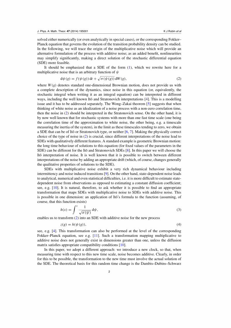
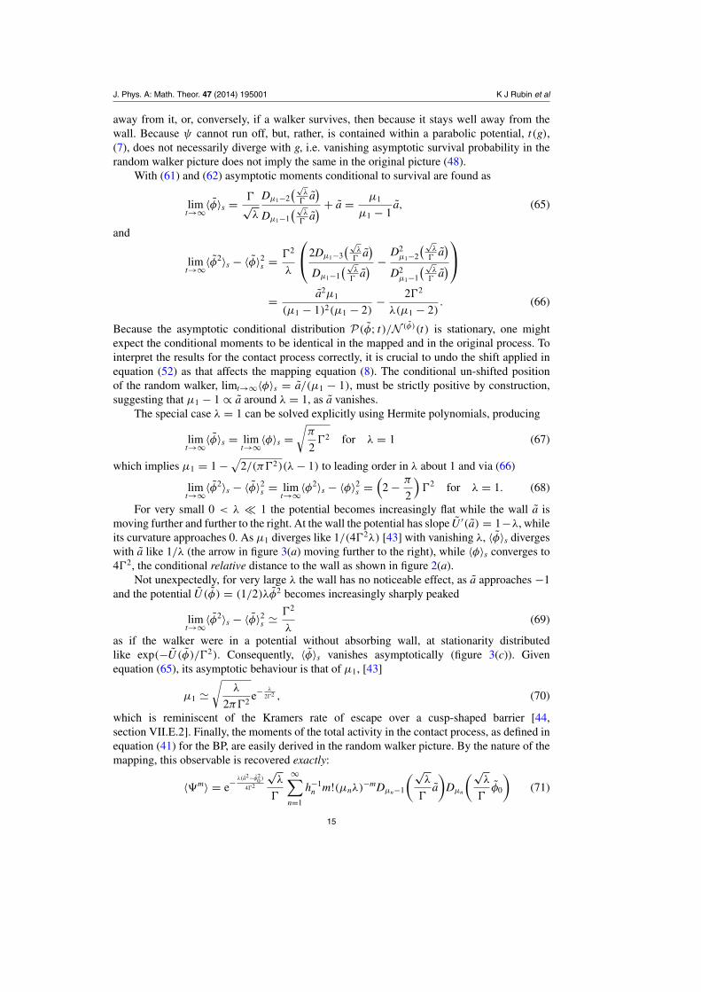
Figure 1. Example of a BP evolving over three generations. The last generation has notyet been updated. The last individual which produced any offspring is the one labelledt = 6. (a) BP as a tree. (b) Mapping of generational time g and individual time t via thegeneration size ψ(g) = φ(t(g)).

theorem [4, theorem 3.4.6], which states that continuous local martingales in one dimensioncan be expressed as time changed Brownian motions, with the new time being the quadraticvariation of the process. For the purposes of this paper, we can state this result as follows:we can find a new Brownian motion W (g), such that the stochastic integral in (the integratedversion of (2)) can be written∫ t

0

√σ (ψ(g)) dW (g) = W

(∫ t

0σ (ψ(g)) dg

). (5)

By construction, this change of the clock works only in one dimension.Just as with the Lamperti transformation (3), this transformation can also be performed at

the level of the Fokker–Planck equation. Even though the Dambis–Dubins–Schwarz theoremis a standard result in stochastic analysis that has been used for the theoretical analysis of SDEsin one dimension (and also for the proof of homogenization theorems with error estimates[12]) it has not been used, to our knowledge, in the calculation of statistical quantities ofinterest for SDEs with multiplicative noise, in particular when boundary conditions have tobe taken into account. More precisely, the connection between the change of the clock at thelevel of the SDE and the study of branching processes (BPs) is not known. It is the goal ofthis paper to study precisely this problem and apply our insight to the analysis of the randomneighbour contact process.

The following section motivates the mapping and (for illustrative purposes) exemplifies itusing a continuum formulation of the branching process. In that case essentially all results areknown in closed form. In section 3 we proceed to apply the mapping to the random neighbourcontact process, which will be turned into an Ornstein–Uhlenbeck process with absorbingwall. Section 4 contains a discussion of the results.

2. Branching process

The mapping employed in the following between a random walk (RW) and a Watson–GaltonBP, is very well established in the literature [13–16]. We adopt the language of a (family)tree, such as the one shown in figure 1. The BP can be studied at two different time scales,the slow generational time g (as the one indicated on the axis in figure 1(a)) and the fastindividual time t which corresponds to the labelling of the nodes shown in figure 1(a). Using

3

J. Phys. A: Math. Theor. 47 (2014) 195001 K J Rubin et al

the mapping as described below, the labelling within a generation and thus the fast time scaleremain somewhat arbitrary, which is irrelevant for the argument.

A branching tree can be considered as having ‘grown’ generation by generation byallowing each individual within a generation to reproduce. In figure 1(a) this is indicatedby the labels of the nodes. If ψ(g) is the number of individuals in generation g, the fast(microscopic) time scale t may be defined as

t(g) =g−1∑g′=0

ψ(g), (6)

namely the total number of reproduction attempts that occurred up to (but excluding) generationg, the slow (macroscopic) time scale. With obvious generalizations in mind, the followingdiscussion is restricted to a BP with two reproduction attempts for each node, implementedby two independent Bernoulli trials with probability p, i.e. two offspring are produced withprobability p2, a single one with 2p(1− p) and none with (1− p)2. In this setup, the evolutionof the BP can be guided by a RW of φ(t) which may change by at most 1 at two consecutivetimes. The population size ψ(g + 1) of generation g + 1 is then determined by φ(t(g + 1))

which has taken ψ(g) time steps since t(g), so that φ(t(g)) = ψ(g). No further evolution cantake place once ψ(g), or, for that matter, φ(t), has vanished. In other words, the RWs to beconsidered are those along an absorbing wall.

Each time step t of the random walker corresponds to a reproduction attempt of anindividual in the previous generation, as indicated by the labelling in figure 1(a), which is notunique, yet can be interpreted as a particular realization of the partial reproduction attempt ofa generation. This picture therefore affords a bijection between RW and BP.

2.1. Continuum formulation

To make further progress, the mapping is re-formulated in the continuum on the basis of thedefinition

t(g) =∫ g

0dg′ψ(g′) (7)

and φ(t(g)) = ψ(g). Since t(0) = 0 the initial conditions used below will be ψ0 = φ0. Tomake equation (7) a bijection, ψ(g) and thus φ(t) may not vanish. Equation (7) is then easilyinverted,

g(t) =∫ t

0dt ′

1

φ(t ′). (8)

If φ(t) has the equation of motion of a random walker along an absorbing wall with driftε, we have

d

dtφ(t) ≡ φ(t) = ε + ξ (t) (9)

where ξ (t) is a noise with correlator

〈ξ (t)ξ (t ′)〉 = 22δ(t − t ′), (10)

with 〈·〉 denoting the ensemble average. From equation (9) followsd

dgψ(g) = dt

dgφ(t) = ψ(g)(ε + ξ (t(g))) (11)

because dtdg = ψ(g) from equation (7). The equation of motion (11) for ψ(g) can be further

simplified by introducing the noise

〈η(g)η(g′)〉 = 22δ(g − g′) = 22δ(t − t ′)dt

dg, (12)

4

J. Phys. A: Math. Theor. 47 (2014) 195001 K J Rubin et al

or, equivalently,

η(g) =√

ψ(g)ξ (t(g)) (13)

which results in the final continuum version of the equation of motion of the branching process1

d

dgψ(g) = ψ(g)ε +

√ψ(g)η(g). (14)

The term√

ψ(g)η(g) reflects the fact that the variance of the size of each generation islinear in its previous size (where the term ‘previous’ reminds us of the Ito interpretation ofequation (14)).

The derivation of the SDE (14) involving multiplicative noise from the one involvingadditive noise, equation (9), is invertible, i.e. (7) implies (9) given (14).

Mathematically, the construction above on the level of a Langevin equation is at besthandwaving: Because the random variable ψ(g) enters into the definition (7) of time t, timeitself becomes a random variable. Worse, the definition of the noise via its correlator inequation (12) involves the random variable dt/dg.

At the level of a Fokker–Planck equation, the transform amounts to a change of variables,yet unlike, say, [17, appendix A], one of the time variable, involving the entire history of therandom variable, equation (7).

2.2. Generalization of the mapping

The mapping performed above can be generalized as follows: a Langevin equation of the form

d

dgψ(g) = μ(ψ(g)) + σ (ψ(g))η(g) (15)

with white noise η(g) as defined in equation (12), is equivalent to

d

dtφ(t) = μ(φ(t))

σ 2(φ(t))+ ξ (t) (16)

for φ(t(g)) = ψ(g) along an absorbing wall,

t(g) =∫ g

0dg′σ 2(ψ(g′)) (17)

and white noise ξ (t) as defined in equation (10). However, the distribution of ψ(g) at fixed gdoes not equal the distribution of φ(t) at fixed t, because the map t(g) involves the history ofψ . Some observables, however, do not change under the mapping and can be used to identifya transition, which is illustrated in section 2.4.

2.3. Fokker–Planck equations and solutions

To understand the meaning and the consequences of the mapping introduced above, we obtainsolutions for the Fokker–Planck equations of both, the RW along an absorbing wall withadditive noise (9) and the BP with multiplicative noise (14). Because for the latter the caseε = 0 can be recovered from the general solution with ε �= 0 only in the form of a limit,and because ε < 0 is qualitatively different from ε > 0, these three cases will be discussedseparately.

1 The continuum version of the BP retains some crucial features of the discrete counterpart, so that, for example,asymptotic population sizes in the latter can be calculated on the basis of the former using suitable effective parameters2 and ε. This carries through even to the total population sizes, �, calculated below.

5

J. Phys. A: Math. Theor. 47 (2014) 195001 K J Rubin et al

It is a textbook exercise to find the Fokker–Planck equation for the random walker alongan absorbing wall, equation (9), which is

∂tP (φ)(φ, t;φ0;2, ε) = 2∂2φP (φ) − ε∂φP (φ), (18)

with P (φ)(φ, t;φ0;2, ε) the probability of finding the walker at φ at time t, given it startedfrom φ0 at t = 0,

limt→0

P (φ)(φ, t;φ0;2, ε) = δ(φ − φ0) (19)

and given the amplitude of the noise 2, equation (10), and the drift ε. The absorbing wallimplies a Dirichlet boundary condition

P (φ)(0, t;φ0;2, ε) = 0 (20)

and φ0 > 0. The solution

P (φ)(φ, t;φ0;2, ε) = 1√4π2t

(e− (φ−εt−φ0 )2

42t − e− (φ−εt+φ0 )2

42t e− φ0ε

2

)(21)

is easily obtained using a mirror charge to find the solution of equation (18) whose ε is gaugedaway using a function γ (say, γ (φ, t) = exp{ ε

22 (x − εt/2)}) and writing P (φ) = γ P (φ), orother methods, e.g. [18].

The Fokker–Planck equation of the continuous BP, equation (14), is

∂gP (ψ)(ψ, g;ψ0;2, ε) = 2∂2ψ (ψP (ψ)) − ε∂ψ (ψP (ψ)) (22)

for ψ > 0, with initial condition, ψ0 = ψ(0) = φ0,

limg→0

P (ψ)(ψ, g;ψ0;2, ε) = δ(ψ − ψ0) . (23)

Its solution is

P (ψ)(ψ, g;ψ0;2, ε) =√

ψ0

ψ

εexp(−εg/2)

2(1 − exp(−εg))I1

(2ε

√ψψ0exp(−εg)

2(1 − exp(−εg))

)

×exp

(− ψexp(−εψ) + ψ0

2(1 − exp(−εg))ε

), (24)

where I1 denotes the modified Bessel function of the first kind. The prefactor ε/(1−exp(−εg))

has two important properties. Firstly, for g > 0 it is positive for all non-vanishing ε. Secondly,taking the limit

limε→0

ε

1 − exp(−εg)= 1

g(25)

recovers the solution of equation (22) for ε = 0,

P (ψ)(ψ, g;ψ0;2, ε = 0) =√

ψ0

ψ

1

2gI1

(2√

ψψ0

2ψ

)e− ψ+ψ0

2g . (26)

In fact, the latter solution is found in tables [19–21]. From that, equation (24) isobtained after a sequence of transforms. Firstly, introducing P (ψ)(ψ, g;ψ0;2, ε) =:R(ψexp(−εψ), ψ2)/ψ simplifies equation (22) to R(x, s) = x exp(−εs/2)R′′(x, s). Inorder to absorb the prefactor, we introduce R(x, s) = −(2/ε)S(x, exp(−εs/2)), so thatS(x, b) = −(2/ε)xS′′(x, b). If P (ψ)(ψ, g;ψ0;2, 0) solves equation (22) with ε = 0, thenS(x, b) = AxP (ψ)(x, b−1;ψ0,−2/ε) with the same boundary and initial condition as above.The initial condition applies at b = 1, the value of exp(−εs/2) at s = 0. Some algebra thenrecovers the full solution equation (24).

6

J. Phys. A: Math. Theor. 47 (2014) 195001 K J Rubin et al

2.4. Comparison of the branching process and the random walker picture

In the following we compare a range of observables between the different processes or, rather,their description. In fact, equations (21) and (24) are only two different perspectives on thesame process, with the advantage that one (the former, with additive noise) is much easier toobtain and analyse than the other.

In the Langevin equations (14) and (9), ψ and φ respectively do not recover from havingvanished. In the following the limits

limt→∞N (φ)(t;φ0;2, ε) = : N (φ)

0 (φ0;2, ε) (27a)

limg→∞N (ψ)(g;ψ0;2, ε) = : N (ψ)

0 (ψ0;2, ε) (27b)

of the integrals

N (φ)(t;φ0;2, ε) :=∫ ∞

0dφP (φ)(φ, t;φ0;2, ε) (28a)

N (ψ)(g;ψ0;2, ε) :=∫ ∞

0dψP (ψ)(ψ, g;ψ0;2, ε) (28b)

are referred to as the asymptotic survival probabilities. Inspecting equation (7) shows thatindefinite survival in the BP may not map to indefinite survival of a random walker if ψ(g′)vanishes fast enough. In turn, if φ(t ′) diverges quickly enough, g(t) in equation (8) mightremain finite in the limit t → ∞. Yet, equation (21) indicates that the distribution of φ(t) iscentred around φ0 − εt and events beyond that scale are exponentially suppressed. Indefinitesurvival of a random walker thus results in (typically logarithmic) divergence of g(t) in t.

We conclude that survival of a random walker corresponds to survival of a correspondingBP and, likewise, early death (at finite g) of a BP corresponds to an early death of a randomwalker (at finite t). One may therefore expect that a transition from asymptotic death toasymptotic survival in one system corresponds to a corresponding transition in the othersystem.

Integrating equations (21) and (24) according to equation (28a) gives

N (φ)(t;φ0;2, ε) = 1

2

(1 − e− εφ0

2

(1 + E

(εt − φ0

2√

2t

))+ E

(εt + φ0

2√

2t

))(29)

and

N (ψ)(g;ψ0;2, ε) =

⎧⎪⎪⎨⎪⎪⎩

1 − exp

(− −ψ0ε

2(1 − exp(−εg))

)for ε �= 0

1 − exp

(−−ψ0

2g

)for ε = 0

(30)

which is again continuous in ε. Taking, however, the long time limits gives

N (φ)

0 (φ0;2, ε) =⎧⎨⎩1 − exp

(−−φ0ε

2

)for ε > 0

0 for ε � 0(31a)

N (ψ)

0 (ψ0;2, ε) =⎧⎨⎩1 − exp

(−−ψ0ε

2

)for ε > 0

0 for ε � 0(31b)

7

J. Phys. A: Math. Theor. 47 (2014) 195001 K J Rubin et al

which is, as expected, in agreement, because ψ0 = φ0. A discrepancy is however expected inthe leading order behaviour in large t and g respectively, for ε � 0, which is, for the randomwalker

N (φ)(t, φ0;2, ε) ∼

⎧⎪⎪⎪⎪⎪⎨⎪⎪⎪⎪⎪⎩

1 − e− −φ0ε

2 for ε > 0 (32a)φ0√π2t

for ε = 0

2φ0

(εt + φ0)(εt − φ0)

√2t

πe− (εt+φ0 )2

42t for ε < 0 (32c)

(32b)

and for the BP

N (ψ)(g, ψ0;2, ε) ∼

⎧⎪⎪⎪⎪⎪⎨⎪⎪⎪⎪⎪⎩

1 − e− ψ0ε

2 for ε > 0 (33a)

ψ0

2gfor ε = 0

ψ0|ε|2

eεg for ε < 0. (33c)

(33b)

The case ε = 0, obviously the critical point, deserves special attention. It is well known thatthe survival probability in a fair BP, ε = 0, is inverse in the number of generations [13]. Sincethe expected population size remains unchanged in the fair case, 〈ψ〉(g, ψ0;2, ε = 0) = ψ0,as discussed below, the expected population size conditional to survival is 2g accordingto equation (33b). On that basis, equation (7) suggests t(g) ≈ (1/2)2g2 which producesφ0/(

2g√

π/2) in (32b), out by a factor 1/√

π/2 compared to the asymptote for the BP atε = 0, equation (33b).

Other observables worth comparing are moments conditional to survival, as they arestationary. The moments

〈ψn〉 =∫ ∞

0dψψnP (ψ)(ψ, g;ψ0;2, ε) (34)

of equation (24) can be calculated very easily using the identity∫ ∞

0dx I1(x) e−γ x2 = e1/(4γ ) − 1 (35)

and differentiating with respect to γ which gives∫ ∞

0dψψ−1/2I1(

√ψα) eβψψn = 2α−(2n+1)

(− d

dγ

)n∣∣∣∣γ=−β/α2

(e1/(4γ ) − 1

). (36)

We find, for example,

〈ψ0〉 = 1 − e− ψ0ε

2 (1−exp(−εg)) (37a)

〈ψ1〉 = ψ0eεg (37b)

〈ψ2〉 = 〈ψ1〉2 + 2ψ02

ε(e2εg − eεg), (37c)

where we use the convention 〈ψ0〉 = N (ψ)(g, ψ0;2, ε) and similarly for φ. Correspondingexpressions for the random walker are extremely messy (as can be seen in equation (29)), sowe state only the first moment (the zeroth moment is stated in equation (29) and its expansionin equation (32b)), dropping lower order terms in t (l.o.t.):

〈φ1〉 =

⎧⎪⎪⎪⎪⎨⎪⎪⎪⎪⎩

εt(

1 − e− εφ02

)+ l.o.t. for ε > 0 (38a)

φ0 for ε = 0

8φ0|ε|2t2

(εt + φ0)2(εt − φ0)2

√2t

πe− (εt+φ0 )2

42t + l.o.t. for ε < 0 (38c)

(38b)

8

J. Phys. A: Math. Theor. 47 (2014) 195001 K J Rubin et al

Normalizing the moments with the respective survival probability gives the momentsconditional to survival, 〈ψn〉s = 〈ψn〉/N (ψ) and similar for 〈φn〉s. For ε > 0 the normalizationis the same in both cases, equation (31a), so a comparison of the conditional momentscomes in fact down to comparison of the unconditional moments. For ψ ≈ ψ0exp(εg)

the mapped time is t(g) = ψ0(exp(εg) − 1)/ε which in equation (38b) gives 〈φ〉 =ψ0(exp(εg) − 1)

(1 − exp

(− εφ0

2

)), not quite matching equation (37b).

For ε = 0 the unconditional moments are identical, equation (37b) (at ε = 0) andequation (38b), so the comparison of the conditional moments is merely a comparison of thenormalizations (32b) and (33b), which has been addressed above.

The case ε < 0 gives a conditional first moment of limt→∞〈φ1〉s = limt→∞〈φ1〉/〈φ0〉 =42/|ε| while the BP gives limg→∞〈ψ1〉s = limg→∞〈ψ1〉/〈ψ0〉 = 2/|ε|.

At first one may expect time independent quantities to be equal in both setups. However,as they remain subject to their dynamics, survivors in one system (say the BP) may generallybe much closer to death than survivors in the other (say the random walkers), as they continueto linger close to extinction.

One observable that can be recovered in the random walker mapping in exact form is thetotal population size2 in the BP

� =∫ ∞

0dg′ψ(g′) (39)

whose expectation is finite if ε < 0 and corresponds, according to the mapping (7), exactly tothe time a random walker hits the absorbing wall. This is easily confirmed for the first moment,since

〈�〉 =∫ ∞

0dg′〈ψ(g′)〉 = ψ0

|ε| (40)

for ε < 0 and because the probability density of walkers to hit the wall at t is(− ∂

∂t )N (φ)(t;φ0;2, ε), in the random walker picture

〈�n〉 =∫ ∞

0dttn

(− ∂

∂t

)N (φ)(t;φ0;2, ε). (41)

One thus easily finds for ε < 0

〈�1〉 = φ0

|ε| (42a)

〈�2〉 = 〈�〉2 + 22φ0

|ε|3 (42b)

〈�3〉 = φ0

|ε5|(124 + 62|ε|φ0 + ε2φ2

0

)= 〈�〉3 + 3(〈�2〉 − 〈�〉2)〈�〉 + 124φ0

|ε5| (42c)

obtained straightforwardly in the random walker picture. In contrast, deriving higher momentsof � in the BP picture is quite cumbersome, as they require higher correlation functions, forexample

〈�2〉 =∫ ∞

0dg′

∫ ∞

0dg′′〈ψ(g′)ψ(g′′)〉. (43)

2 In self-organized criticality the total population size is in fact the time-integrated activity or, equivalently, theavalanche size [22].

9

J. Phys. A: Math. Theor. 47 (2014) 195001 K J Rubin et al

In the presence of the ‘kernel’ P (ψ), equation (24), this correlation function is determined via

〈ψ(g′)ψ(g′′)〉 =∫ ∞

0dψ ′ψ ′P (ψ)(ψ ′, g′;ψ0;2, ε)

∫ ∞

0dψ ′′ψ ′′P (ψ)(ψ ′′, g′′ − g′;ψ ′;2, ε)

(44)

assuming g′′ > g′. The resulting expressions can be evaluated using the moments calculatedabove, equations (37a)–(37c). As expected, they exactly coincide with equations (42a)–(42c).

3. Contact process

We will now use the mapping illustrated above to characterize the stochastic equation ofmotion of the random neighbour contact process.

The contact process [1] is a simple lattice model, for example of the spatio-temporalevolution of an immobile plant species spreading on a substrate. For definiteness set up on asquare lattice, sites are either occupied or empty. Occupied sites become empty with Poissonianextinction rate e and attempt to occupy with an offspring each of their neighbouring sites withthe same rate c/q, where q is the number of neighbours, in case of nearest neighbour interaction,q being the coordination number. Such an attempt is successful, resulting in occupation ofthe empty site, only when the targeted site was empty prior to the attempt. The interactionis thus due to excluded volume, as colonization can occur only at empty sites. Sites becomeoccupied with Poissonian colonization rate kc/q, where k is the number of occupied nearestneighbours. Extensions to higher and lower dimensions are obvious. Rescaling the time by edetermines the single parameter controlling the dynamics as λ = c/e. It turns out [23] that inthe thermodynamic limit a finite population density of occupied sites ψ is sustained for all λ

greater than some λc, displaying all features of a second order phase transition [24].In fact, these features can already be seen in a mean field theory, where the rise in

occupation density is given by the competition of extinction and global colonization as afunction of time g

d

dgψ = λ(1 − ψ)ψ − ψ (45)

which has a non-trivial stationary state ψ = 1 − 1/λ > 0 for λ > 1, i.e. λc = 1. In fact, toleading order ψ ∝ (λ − λc)

−1 for λ � λc and ψ = 0 otherwise. To go beyond mean fieldtheory, two additional ingredients are needed, namely spatial interaction and noise. The formeris implemented by smoothing out the occupation by introducing a diffusion term. The latteraccounts for the stochastic nature of the process. Similar to the BP analysed in section 2, thevariance of fluctuations should be linear in the local occupation. The full Langevin equationof motion that is usually analysed as the contact process [1] reads3

ψ (x, g) = λ(1 − ψ(x, g))ψ(x, g) − ψ(x, g) + D∇2ψ +√

ψ(x, t)η(x, g) (46)

where the noise has vanishing mean, is Gaussian, white and has correlator

〈η(x, g)η(x′, g′)〉 = 22δ(g − g′)δ(x − x′). (47)

This equation has been analysed extensively using field theoretic methods [25–27], inparticular perturbation theory. Above the upper critical dimension d > dc = 4 [28, 29] spatial

3 The absence of an explicit carrying capacity and extinction rate spoils the usual dimensional independence of ψ .

10

J. Phys. A: Math. Theor. 47 (2014) 195001 K J Rubin et al

φ

U

〈φ〉s

(a) λ = 1/2

φ

U

〈φ〉s

(b) λ = 1

φ

U

〈φ〉s

(c) λ = 3

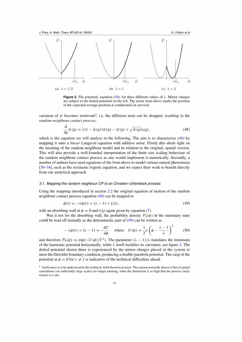
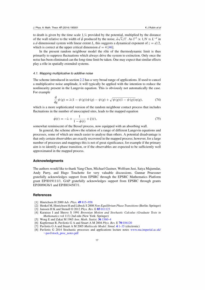
Figure 2. The potential, equation (50), for three different values of λ. Mirror chargesare subject to the dotted potential on the left. The arrow from above marks the positionof the expected average position φ conditioned on survival.

variation of ψ becomes irrelevant4, i.e. the diffusion term can be dropped, resulting in therandom neighbour contact process,

d

dgψ(g) = λ(1 − ψ(g))ψ(g) − ψ(g) +

√ψ(g)η(g), (48)

which is the equation we will analyse in the following. The aim is to characterize (48) bymapping it onto a linear Langevin equation with additive noise. Firstly this sheds light onthe meaning of the random neighbour model and its relation to the original, spatial version.This will also provide a well-founded interpretation of the finite size scaling behaviour ofthe random neighbour contact process as one would implement it numerically. Secondly, anumber of authors have used equations of the form above to model various natural phenomena[30–34], such as the stochastic logistic equation, and we expect their work to benefit directlyfrom our analytical approach.

3.1. Mapping the random neighbour CP to an Ornstein–Uhlenbeck process

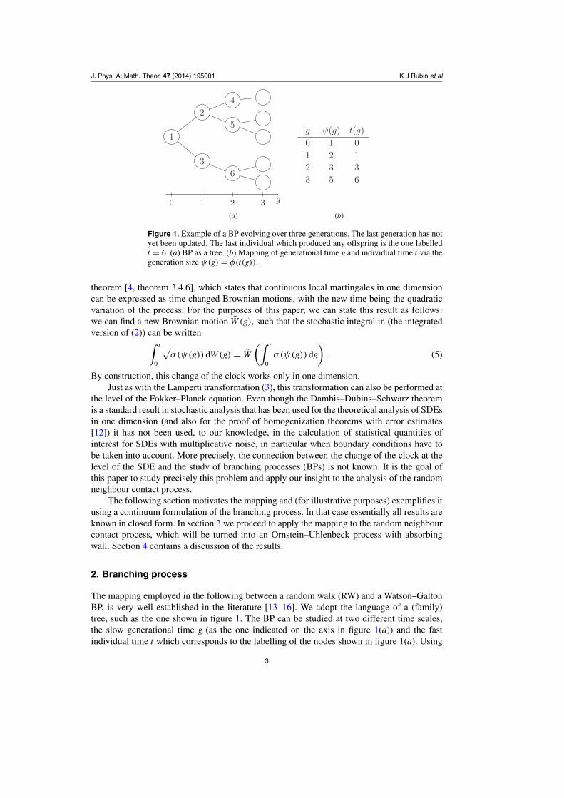
Using the mapping introduced in section 2.2 the original equation of motion of the randomneighbour contact process equation (48) can be mapped to

φ(t) = −λφ(t) + (λ − 1) + ξ (t), (49)

with an absorbing wall at φ = 0 and t(g) again given by equation (7).Was it not for the absorbing wall, the probability density P0(φ) in the stationary state

could be read off instantly as the deterministic part of (49) can be written as

− λφ(t) + (λ − 1) = −dU

dφwhere U (φ) = 1

2λ

(φ − λ − 1

λ

)2

(50)

and therefore P0(φ) ∝ exp(−U (φ)/2). The parameter (λ − 1)/λ translates the minimumof the harmonic potential horizontally, while λ itself modifies its curvature, see figure 2. Thedotted potential shown there is experienced by the mirror charges placed in the system tomeet the Dirichlet boundary condition, producing a double-parabola potential. The cusp of thepotential at φ = 0 for λ �= 1 is indicative of the technical difficulties ahead.

4 Irrelevance is to be understood in the technical, field-theoretical sense. The cartoon normally drawn is that of spatialcorrelations (on sufficiently large scales) no longer entering, when the dimension is so high that the process rarelyreturns to a site.

11

J. Phys. A: Math. Theor. 47 (2014) 195001 K J Rubin et al

φ

U

⟨φ⟩

s

(a) λ = 1/2, a = 1

φ

U

⟨φ⟩

s

(b) λ = 1, a = 0

φ

U

⟨φ⟩

s

(c) λ = 3, a = −2/3

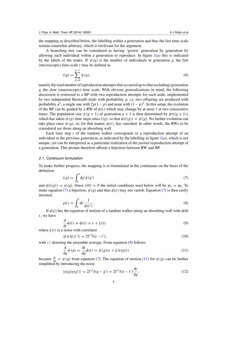
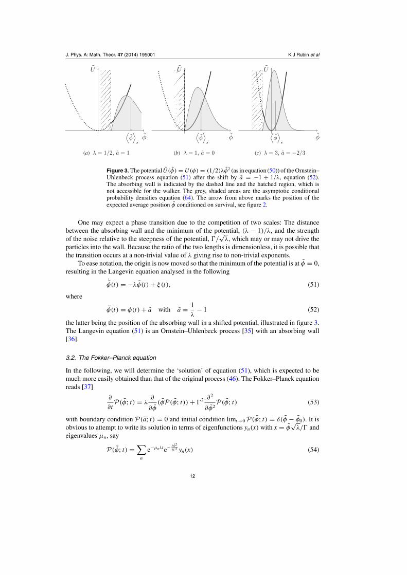
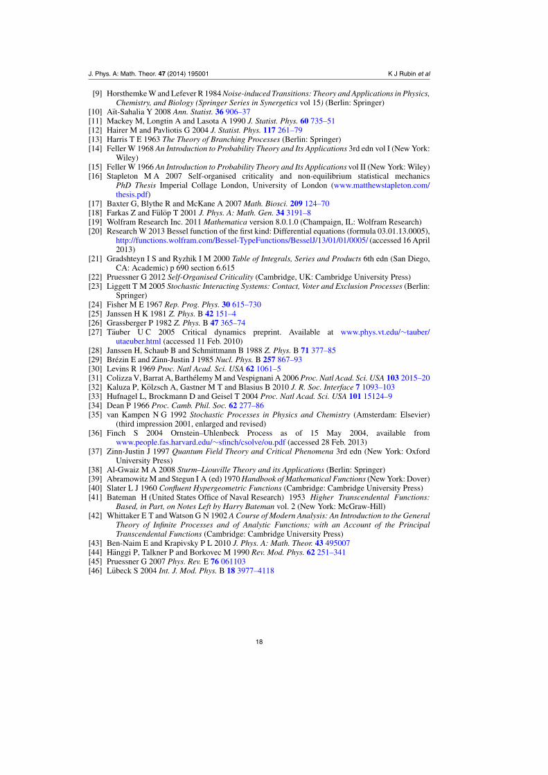
Figure 3. The potential U (φ) = U (φ) = (1/2)λφ2 (as in equation (50)) of the Ornstein–Uhlenbeck process equation (51) after the shift by a = −1 + 1/λ, equation (52).The absorbing wall is indicated by the dashed line and the hatched region, which isnot accessible for the walker. The grey, shaded areas are the asymptotic conditionalprobability densities equation (64). The arrow from above marks the position of theexpected average position φ conditioned on survival, see figure 2.

One may expect a phase transition due to the competition of two scales: The distancebetween the absorbing wall and the minimum of the potential, (λ − 1)/λ, and the strengthof the noise relative to the steepness of the potential, /

√λ, which may or may not drive the

particles into the wall. Because the ratio of the two lengths is dimensionless, it is possible thatthe transition occurs at a non-trivial value of λ giving rise to non-trivial exponents.

To ease notation, the origin is now moved so that the minimum of the potential is at φ = 0,resulting in the Langevin equation analysed in the following

˙φ(t) = −λφ(t) + ξ (t), (51)

where

φ(t) = φ(t) + a with a = 1

λ− 1 (52)

the latter being the position of the absorbing wall in a shifted potential, illustrated in figure 3.The Langevin equation (51) is an Ornstein–Uhlenbeck process [35] with an absorbing wall[36].

3.2. The Fokker–Planck equation

In the following, we will determine the ‘solution’ of equation (51), which is expected to bemuch more easily obtained than that of the original process (46). The Fokker–Planck equationreads [37]

∂

∂tP(φ; t) = λ

∂

∂φ(φP(φ; t)) + 2 ∂2

∂φ2P(φ; t) (53)

with boundary condition P(a; t) = 0 and initial condition limt→0 P(φ; t) = δ(φ − φ0). It isobvious to attempt to write its solution in terms of eigenfunctions yn(x) with x = φ

√λ/ and

eigenvalues μn, say

P(φ; t) =∑

n

e−μnλte− λφ2

22 yn(x) (54)

12

J. Phys. A: Math. Theor. 47 (2014) 195001 K J Rubin et al

where yn fulfils the eigenvalues equation

y′′n − xy′

n = −μnyn, (55)

with yn(a) = 0. The factor exp(−λφ2/(22)) in (54) appears quite naturally; without it, theeigenvalues μn were negative and each term in the series divergent. Equation (55) is in factthe eigenvalue problem of the Kolmogorov backward operator (generator) [9] of (53) and forμn ∈ N (55) is the Hermite equation.

However, Hermite polynomials do not generally solve (55), because they do not generallyfulfil yn(a) = 0, except when a = 0 (i.e. the potential in figure 2(a) without a cusp), whereyn(x) = Hm(x) for n = 0, 1, 2, . . . and m = 2n + 1, so that μn = m. This solution in oddpolynomials hints at the interpretation of the problem in terms of a mirror charge trick alludedto earlier.

The Kolmogorov backward equation (55) is also a Sturm–Liouville eigenvalue problemand multiplication by the weight function e− x2

2 converts it to standard Sturm–Liouville form

(e− x2

2 y′n(x))′ + μne− x2

2 yn(x) = 0. (56)

A Sturm–Liouville eigenvalue problem has a set of eigenvalues corresponding to a completeset of orthogonal eigenfunctions that are square integrable with respect to the weight function[38]. This equation is a singular Sturm–Liouville problem because it is defined on an infinite

interval and therefore an extra condition is needed such that

√e− x2

2 yn(x) tends to zero as|x| −→ ∞, to ensure square integrability of yn(x). If this condition holds then a complete setof solutions can be found.

Solutions of (55) can be constructed in terms of a series by studying the recurrence relationof its coefficients. A more efficient route is the use of special functions, such as confluenthypergeometric functions also known as Kummer functions [39]. These are solutions of thedifferential equation [40] x d2y

dx2 + (β − x)dydx − αy = 0 where y(x) = M(α;β; x) or y(x) =

U(α;β; x) or any linear combination thereof. A solution of the form y = U(−μn/2; 1/2; x2/2)

solves equation (55) and satisfies the Dirichlet boundary condition at a for suitably chosen μn.It turns out that of the two independent solutions, only U has the right asymptotic behaviour inlarge x to guarantee square integrability. Unfortunately, U(−μn/2; 1/2; x2/2) does not solvethe equation for a < 0 because it has a singularity at zero and can therefore not constitute acomplete system of eigenfunctions of the Sturm–Liouville problem.

Another differential equation to consider is the parabolic cylinder function equationd2y

dx2+

(ν + 1

2− x2

4

)y = 0. (57)

The solutions of this equation [41] are the parabolic cylinder functions y(x) = Dν (x),which also solve equation (55) when of the form y = e

x2

4 Dν (x), specifically Dν (x) =exp(−x2/4)Hν (x) for integer ν. For suitable μn the parabolic cylinder functions satisfy theboundary condition at a, namely Dμn (a

√λ/) = 0, and are analytic along the whole real line

[42]. The solution of (53) with an absorbing wall at a is thus

P(φ; t) = e− λ(φ2−φ20 )

42

√λ

∞∑n=1

h−1n e−μnλtDμn

(√λ

φ

)Dμn

(√λ

φ0

)(58)

where h−1n is a normalization constant,∫ ∞

a√

λ/

dxDμn (x)Dμm (x) = hnδnm (59)

which holds for any pair μn, μm such that Dμn,m (a√

λ/) = 0. Completeness of Dμn (x)

guarantees the initial condition limt→0 P(φ; t) = δ(φ − φ0).

13

J. Phys. A: Math. Theor. 47 (2014) 195001 K J Rubin et al

0.5 1.0 1.5 2.0 2.5 3.0

1.0

2.0

3.0

4.0

λ

a

μ1λμ1

Figure 4. The smallest eigenvalue μ1 (dotted),i.e. the smallest root μ of Dμ(a√

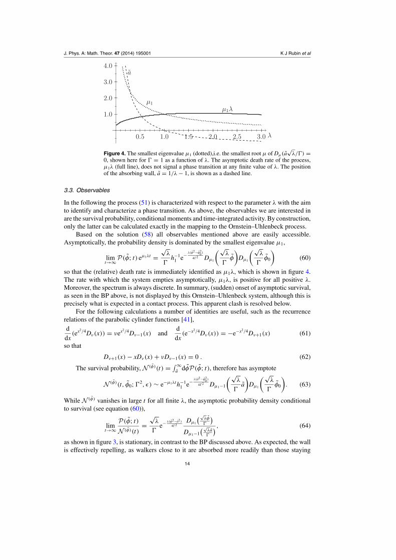
λ/) =0, shown here for = 1 as a function of λ. The asymptotic death rate of the process,μ1λ (full line), does not signal a phase transition at any finite value of λ. The positionof the absorbing wall, a = 1/λ − 1, is shown as a dashed line.

3.3. Observables

In the following the process (51) is characterized with respect to the parameter λ with the aimto identify and characterize a phase transition. As above, the observables we are interested inare the survival probability, conditional moments and time-integrated activity. By construction,only the latter can be calculated exactly in the mapping to the Ornstein–Uhlenbeck process.

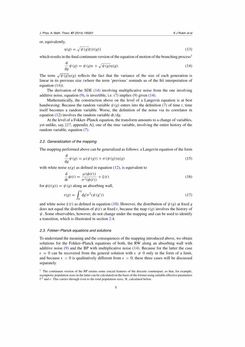
Based on the solution (58) all observables mentioned above are easily accessible.Asymptotically, the probability density is dominated by the smallest eigenvalue μ1,

limt→∞P(φ; t) eμ1λt =

√λ

h−1

1 e− λ(φ2−φ20 )

42 Dμ1

(√λ

φ

)Dμ1

(√λ

φ0

)(60)

so that the (relative) death rate is immediately identified as μ1λ, which is shown in figure 4.The rate with which the system empties asymptotically, μ1λ, is positive for all positive λ.Moreover, the spectrum is always discrete. In summary, (sudden) onset of asymptotic survival,as seen in the BP above, is not displayed by this Ornstein–Uhlenbeck system, although this isprecisely what is expected in a contact process. This apparent clash is resolved below.

For the following calculations a number of identities are useful, such as the recurrencerelations of the parabolic cylinder functions [41],d

dx(ex2/4Dν (x)) = νex2/4Dν−1(x) and

d

dx(e−x2/4Dν (x)) = −e−x2/4Dν+1(x) (61)

so that

Dν+1(x) − xDν (x) + νDν−1(x) = 0 . (62)

The survival probability, N (φ)(t) = ∫ ∞a dφP(φ; t), therefore has asymptote

N (φ)(t, φ0;2, ε) ∼ e−μ1λth−11 e− λ(a2−φ2

0 )

42 Dμ1−1

(√λ

a

)Dμ1

(√λ

φ0

). (63)

While N (φ) vanishes in large t for all finite λ, the asymptotic probability density conditionalto survival (see equation (60)),

limt→∞

P(φ; t)

N (φ)(t)=

√λ

e− λ(φ2−a2 )

42Dμ1

(√λφ

)Dμ1−1

(√λa

) , (64)

as shown in figure 3, is stationary, in contrast to the BP discussed above. As expected, the wallis effectively repelling, as walkers close to it are absorbed more readily than those staying

14

J. Phys. A: Math. Theor. 47 (2014) 195001 K J Rubin et al

away from it, or, conversely, if a walker survives, then because it stays well away from thewall. Because ψ cannot run off, but, rather, is contained within a parabolic potential, t(g),(7), does not necessarily diverge with g, i.e. vanishing asymptotic survival probability in therandom walker picture does not imply the same in the original picture (48).

With (61) and (62) asymptotic moments conditional to survival are found as

limt→∞〈φ〉s = √

λ

Dμ1−2(√

λ

a)

Dμ1−1(√

λ

a) + a = μ1

μ1 − 1a, (65)

and

limt→∞〈φ2〉s − 〈φ〉2

s = 2

λ

⎛⎝2Dμ1−3

(√λ

a)

Dμ1−1(√

λ

a) − D2

μ1−2

(√λ

a)

D2μ1−1

(√λ

a)⎞⎠

= a2μ1

(μ1 − 1)2(μ1 − 2)− 22

λ(μ1 − 2). (66)

Because the asymptotic conditional distribution P(φ; t)/N (φ)(t) is stationary, one mightexpect the conditional moments to be identical in the mapped and in the original process. Tointerpret the results for the contact process correctly, it is crucial to undo the shift applied inequation (52) as that affects the mapping equation (8). The conditional un-shifted positionof the random walker, limt→∞〈φ〉s = a/(μ1 − 1), must be strictly positive by construction,suggesting that μ1 − 1 ∝ a around λ = 1, as a vanishes.

The special case λ = 1 can be solved explicitly using Hermite polynomials, producing

limt→∞〈φ〉s = lim

t→∞〈φ〉s =√

π

22 for λ = 1 (67)

which implies μ1 = 1 −√

2/(π2)(λ − 1) to leading order in λ about 1 and via (66)

limt→∞〈φ2〉s − 〈φ〉2

s = limt→∞〈φ2〉s − 〈φ〉2

s =(

2 − π

2

)2 for λ = 1. (68)

For very small 0 < λ � 1 the potential becomes increasingly flat while the wall a ismoving further and further to the right. At the wall the potential has slope U ′(a) = 1−λ, whileits curvature approaches 0. As μ1 diverges like 1/(42λ) [43] with vanishing λ, 〈φ〉s divergeswith a like 1/λ (the arrow in figure 3(a) moving further to the right), while 〈φ〉s converges to42, the conditional relative distance to the wall as shown in figure 2(a).

Not unexpectedly, for very large λ the wall has no noticeable effect, as a approaches −1and the potential U (φ) = (1/2)λφ2 becomes increasingly sharply peaked

limt→∞〈φ2〉s − 〈φ〉2

s � 2

λ(69)

as if the walker were in a potential without absorbing wall, at stationarity distributedlike exp(−U (φ)/2). Consequently, 〈φ〉s vanishes asymptotically (figure 3(c)). Givenequation (65), its asymptotic behaviour is that of μ1, [43]

μ1 �√

λ

2π2e− λ

22 , (70)

which is reminiscent of the Kramers rate of escape over a cusp-shaped barrier [44,section VII.E.2]. Finally, the moments of the total activity in the contact process, as defined inequation (41) for the BP, are easily derived in the random walker picture. By the nature of themapping, this observable is recovered exactly:

〈�m〉 = e− λ(a2−φ20 )

42

√λ

∞∑n=1

h−1n m!(μnλ)−mDμn−1

(√λ

a

)Dμn

(√λ

φ0

)(71)

15

J. Phys. A: Math. Theor. 47 (2014) 195001 K J Rubin et al

The factor h−1n on the right-hand side ensures quick convergence of the sum. There is, in fact,

no suggestion that 〈�m〉 is not analytic in λ.This concludes the calculation of the observables that are easily derived from the random

walker picture of the random neighbour contact process. The moments of the total activity,(71), are exact, while the moments of the asymptotic conditional population density, such as(67) and (68), are not necessarily. None of the observables, however, signals a transition, incontrast to the simplified mean field theory (45).

4. Discussion and conclusion

Before we discuss the mapping employed above in broader terms, we want to address thequestion of why the random neighbour contact process, as formulated in equation (48), doesnot display the phase transition its mean-field theory exhibits.

The analysis above shows that in the random walker picture, fluctuations will eventuallydrive the particle into the absorbing wall irrespective of its position and the particle’sstarting point. Correspondingly, in the original random neighbour contact process, the activityeventually ceases with finite rate as long as the absorbing state is accessible. On the other hand,every naıve numerical implementation of the random walker contact process will display themean field behaviour. Yet, numerical implementations of absorbing state phase transitionssuffer from the problem of being necessarily finite [45]. Taking the thermodynamic limit iscrucial for the recovery of the transition, because in any finite system the system almost surelyfalls into an absorbing state (extinction). At closer inspection, the same applies in the presentmodel: In increasingly large systems with volume N the effective noise amplitude vanisheslike 2 ∝ 1/N, because the occupation density ψ in a large system is less affected by the noisethan in small systems. Decreasing has the same effect on μn as increasing the magnitude ofa√

λ, since Dμn (a√

λ/) = 0. In the limit of vanishing there are thus three cases:

lim→0

μ1 =

⎧⎪⎨⎪⎩

∞ for a√

λ > 0 (72a)

1 for a√

λ = 0

0 for a√

λ < 0. (72c)

(72b)

It is obviously important to take the limit → 0 in equation (58) before considering itsasymptotes in large t. For a < 0 the particles are pinched in an infinitely sharp potential andcannot overcome the barrier to the absorbing wall, i.e. limt→∞ lim→0〈φ〉 = −a, or accordingto equation (65)

lim→0

〈φ〉s = lim→0

1

μ1 − 1a = −a = 1 − 1

λfor λ > 1 (73)

as a√

λ < 0 in equation (72b), reproducing the mean field result stated after equation (45).The wall becomes accessible for a � 0 in which case limt→∞〈φ〉s = 0. For a

√λ > 0 this

is in line with equations (72b) and (65). For a = 0 the special case (67) applies (becauseλ = 1) and taking the limit 2 → 0 there, produces again 〈φ〉s = 0. The limit → 0 thusrecovers the case = 0 which leads to the mean field theory equation (45) that displays thetransition. Taking the limit → 0 directly in equation (58) using equation (72b) is moredifficult, because we were unable to identify a suitable asymptotic behaviour of Dμ1 (φ

√λ/)

as μ1 approaches 0 and vanishes.In summary, the phase transition disappears provided the amplitude of the noise correlator

is finite, because all walkers will eventually reach the absorbing wall, irrespective of the valueof λ. The transition can thus be partly restored by studying finite t, as the characteristic time

16

J. Phys. A: Math. Theor. 47 (2014) 195001 K J Rubin et al

to death is given by the time scale 1/λ provided by the potential, multiplied by the distanceof the wall relative to the width of φ produced by the noise, a

√λ/. As 2 ∝ 1/N ∝ L−d in

a d-dimensional system with linear extent L, this suggests a dynamical exponent of z = d/2,which is correct at the upper critical dimension d = 4 [46].

In the present random neighbour model the role of the thermodynamic limit is thusprimarily to suppress fluctuations which always drive the system to extinction. Only once thenoise has been eliminated can the long-time limit be taken. One may expect that similar effectsplay a role in spatially extended systems.

4.1. Mapping multiplicative to additive noise

The scheme introduced in section 2.2 has a very broad range of applications. If used to cancela multiplicative noise amplitude, it will typically be applied with the intention to reduce thenonlinearity present in the Langevin equation. This is obviously not automatically the case.For example

d

dgψ(g) = λ(1 − ψ(g))ψ(g) − ψ(g) +

√ψ(g)(1 − ψ(g))η(g), (74)

which is a more sophisticated version of the random neighbour contact process that includesfluctuations in the number of unoccupied sites, leads to the mapped equation

φ(t) = −λ + 1

1 − φ(t)+ ξ (t), (75)

somewhat reminiscent of the Bessel process, now equipped with an absorbing wall.In general, the scheme allows the relation of a range of different Langevin equations and

processes, some of which are much easier to analyse than others. A potential disadvantage isthat only certain observables are exactly recovered in the mapped process; however, for a largenumber of processes and mappings this is not of great significance, for example if the primaryaim is to identify a phase transition, or if the observables are expected to be sufficiently wellapproximated in the mapped process.

Acknowledgments

The authors would like to thank Yang Chen, Michael Gastner, Wolfram Just, Satya Majumdar,Andy Parry, and Hugo Touchette for very valuable discussions. Gunnar Pruessnergratefully acknowledges support from EPSRC through the EPSRC Mathematics Platformgrant EP/I019111/1. GAP gratefully acknowledges support from EPSRC through grantsEP/J009636/1 and EP/H034587/1.

References

[1] Hinrichsen H 2000 Adv. Phys. 49 815–958[2] Henkel M, Hinrichsen H and Lubeck S 2008 Non-Equilibrium Phase Transitions (Berlin: Springer)[3] Janssen H K and Stenull O 2012 Phys. Rev. E 85 011123[4] Karatzas I and Shreve S 1991 Brownian Motion and Stochastic Calculus (Graduate Texts in

Mathematics vol 113) 2nd edn (New York: Springer)[5] Wong E and Zakai M 1965 Ann. Math. Statist. 36 1560–4[6] Kupferman R, Pavliotis G A and Stuart A M 2004 Phys. Rev. E 70 036120[7] Pavliotis G A and Stuart A M 2005 Multiscale Model. Simul. 4 1–35 (electronic)[8] Pavliotis G 2014 Stochastic processes and applications lecture notes www.ma.imperial.ac.uk/

∼pavl/stoch_proc_notes.pdf

17

J. Phys. A: Math. Theor. 47 (2014) 195001 K J Rubin et al

[9] Horsthemke W and Lefever R 1984 Noise-induced Transitions: Theory and Applications in Physics,Chemistry, and Biology (Springer Series in Synergetics vol 15) (Berlin: Springer)

[10] Aıt-Sahalia Y 2008 Ann. Statist. 36 906–37[11] Mackey M, Longtin A and Lasota A 1990 J. Statist. Phys. 60 735–51[12] Hairer M and Pavliotis G 2004 J. Statist. Phys. 117 261–79[13] Harris T E 1963 The Theory of Branching Processes (Berlin: Springer)[14] Feller W 1968 An Introduction to Probability Theory and Its Applications 3rd edn vol I (New York:

Wiley)[15] Feller W 1966 An Introduction to Probability Theory and Its Applications vol II (New York: Wiley)[16] Stapleton M A 2007 Self-organised criticality and non-equilibrium statistical mechanics

PhD Thesis Imperial Collage London, University of London (www.matthewstapleton.com/thesis.pdf)

[17] Baxter G, Blythe R and McKane A 2007 Math. Biosci. 209 124–70[18] Farkas Z and Fulop T 2001 J. Phys. A: Math. Gen. 34 3191–8[19] Wolfram Research Inc. 2011 Mathematica version 8.0.1.0 (Champaign, IL: Wolfram Research)[20] Research W 2013 Bessel function of the first kind: Differential equations (formula 03.01.13.0005),

http://functions.wolfram.com/Bessel-TypeFunctions/BesselJ/13/01/01/0005/ (accessed 16 April2013)

[21] Gradshteyn I S and Ryzhik I M 2000 Table of Integrals, Series and Products 6th edn (San Diego,CA: Academic) p 690 section 6.615

[22] Pruessner G 2012 Self-Organised Criticality (Cambridge, UK: Cambridge University Press)[23] Liggett T M 2005 Stochastic Interacting Systems: Contact, Voter and Exclusion Processes (Berlin:

Springer)[24] Fisher M E 1967 Rep. Prog. Phys. 30 615–730[25] Janssen H K 1981 Z. Phys. B 42 151–4[26] Grassberger P 1982 Z. Phys. B 47 365–74[27] Tauber U C 2005 Critical dynamics preprint. Available at www.phys.vt.edu/∼tauber/

utaeuber.html (accessed 11 Feb. 2010)[28] Janssen H, Schaub B and Schmittmann B 1988 Z. Phys. B 71 377–85[29] Brezin E and Zinn-Justin J 1985 Nucl. Phys. B 257 867–93[30] Levins R 1969 Proc. Natl Acad. Sci. USA 62 1061–5[31] Colizza V, Barrat A, Barthelemy M and Vespignani A 2006 Proc. Natl Acad. Sci. USA 103 2015–20[32] Kaluza P, Kolzsch A, Gastner M T and Blasius B 2010 J. R. Soc. Interface 7 1093–103[33] Hufnagel L, Brockmann D and Geisel T 2004 Proc. Natl Acad. Sci. USA 101 15124–9[34] Dean P 1966 Proc. Camb. Phil. Soc. 62 277–86[35] van Kampen N G 1992 Stochastic Processes in Physics and Chemistry (Amsterdam: Elsevier)

(third impression 2001, enlarged and revised)[36] Finch S 2004 Ornstein–Uhlenbeck Process as of 15 May 2004, available from

www.people.fas.harvard.edu/∼sfinch/csolve/ou.pdf (accessed 28 Feb. 2013)[37] Zinn-Justin J 1997 Quantum Field Theory and Critical Phenomena 3rd edn (New York: Oxford

University Press)[38] Al-Gwaiz M A 2008 Sturm–Liouville Theory and its Applications (Berlin: Springer)[39] Abramowitz M and Stegun I A (ed) 1970 Handbook of Mathematical Functions (New York: Dover)[40] Slater L J 1960 Confluent Hypergeometric Functions (Cambridge: Cambridge University Press)[41] Bateman H (United States Office of Naval Research) 1953 Higher Transcendental Functions:

Based, in Part, on Notes Left by Harry Bateman vol. 2 (New York: McGraw-Hill)[42] Whittaker E T and Watson G N 1902 A Course of Modern Analysis: An Introduction to the General

Theory of Infinite Processes and of Analytic Functions; with an Account of the PrincipalTranscendental Functions (Cambridge: Cambridge University Press)

[43] Ben-Naim E and Krapivsky P L 2010 J. Phys. A: Math. Theor. 43 495007[44] Hanggi P, Talkner P and Borkovec M 1990 Rev. Mod. Phys. 62 251–341[45] Pruessner G 2007 Phys. Rev. E 76 061103[46] Lubeck S 2004 Int. J. Mod. Phys. B 18 3977–4118

18