mapping and assessment of the united states ocean wave

2011 TECHNICAL REPORT

Electric Power Research Institute 3420 Hillview Avenue, Palo Alto, California 94304-1338 • PO Box 10412, Palo Alto, California 94303-0813 USA

800.313.3774 • 650.855.2121 • [email protected] • www.epri.com

Mapping and Assessment of the United States Ocean Wave Energy Resource

EPRI Project Manager P. Jacobson

3420 Hillview Avenue Palo Alto, CA 94304-1338 USA PO Box 10412 Palo Alto, CA 94303-0813 USA 800.313.3774 650.855.2121

[email protected] 1024637

www.epri.com Final Report, December 2011

Mapping and Assessment of the United States Ocean Wave Energy Resource

mailto:[email protected]�

http://www.epri.com/�

DISCLAIMER OF WARRANTIES AND LIMITATION OF LIABILITIES

THIS DOCUMENT WAS PREPARED BY THE ORGANIZATION(S) NAMED BELOW AS AN ACCOUNT OF WORK SPONSORED OR COSPONSORED BY THE ELECTRIC POWER RESEARCH INSTITUTE, INC. (EPRI). NEITHER EPRI, ANY MEMBER OF EPRI, ANY COSPONSOR, THE ORGANIZATION(S) BELOW, NOR ANY PERSON ACTING ON BEHALF OF ANY OF THEM:

(A) MAKES ANY WARRANTY OR REPRESENTATION WHATSOEVER, EXPRESS OR IMPLIED, (I) WITH RESPECT TO THE USE OF ANY INFORMATION, APPARATUS, METHOD, PROCESS, OR SIMILAR ITEM DISCLOSED IN THIS DOCUMENT, INCLUDING MERCHANTABILITY AND FITNESS FOR A PARTICULAR PURPOSE, OR (II) THAT SUCH USE DOES NOT INFRINGE ON OR INTERFERE WITH PRIVATELY OWNED RIGHTS, INCLUDING ANY PARTY'S INTELLECTUAL PROPERTY, OR (III) THAT THIS DOCUMENT IS SUITABLE TO ANY PARTICULAR USER'S CIRCUMSTANCE; OR

(B) ASSUMES RESPONSIBILITY FOR ANY DAMAGES OR OTHER LIABILITY WHATSOEVER (INCLUDING ANY CONSEQUENTIAL DAMAGES, EVEN IF EPRI OR ANY EPRI REPRESENTATIVE HAS BEEN ADVISED OF THE POSSIBILITY OF SUCH DAMAGES) RESULTING FROM YOUR SELECTION OR USE OF THIS DOCUMENT OR ANY INFORMATION, APPARATUS, METHOD, PROCESS, OR SIMILAR ITEM DISCLOSED IN THIS DOCUMENT.

REFERENCE HEREIN TO ANY SPECIFIC COMMERCIAL PRODUCT, PROCESS, OR SERVICE BY ITS TRADE NAME, TRADEMARK, MANUFACTURER, OR OTHERWISE, DOES NOT NECESSARILY CONSTITUTE OR IMPLY ITS ENDORSEMENT, RECOMMENDATION, OR FAVORING BY EPRI.

THE FOLLOWING ORGANIZATION(S), UNDER CONTRACT TO EPRI, PREPARED THIS REPORT:

Virginia Tech Advanced Research Institute

National Renewable Energy Laboratory

NOTE

For further information about EPRI, call the EPRI Customer Assistance Center at 800.313.3774 or e-mail [email protected].

Electric Power Research Institute, EPRI, and TOGETHER…SHAPING THE FUTURE OF ELECTRICITY are registered service marks of the Electric Power Research Institute, Inc.

Copyright © 2011 Electric Power Research Institute, Inc. All rights reserved.

This publication is a corporate document that should be cited in the

literature in the following manner:

Mapping and Assessment of the United States Ocean Wave

Energy Resource. EPRI, Palo Alto, CA: 2011.

1024637.

iii

Acknowledgments The following organization, under contract to the Electric Power Research Institute (EPRI), prepared this report:

Virginia Tech Advanced Research Institute 900 North Glebe Road Arlington, VA 22203

Principal Investigator G. Hagerman

National Renewable Energy Laboratory 1617 Cole Blvd. Golden, CO 80401

Principal Investigator G. Scott

This report describes research sponsored by EPRI.

EPRI would like to thank participants in the expert and user group workshops who contributed their expertise during the course of this project, including: Jochen Bard, University of Kassel; Steve Barstow, Fugro Oceanor; Greg Beaudoin, Strategic Insight Ltd.; Stuart Bensly, Oceanlinx; Stephen Bowler, Federal Energy Regulatory Commission; Garth Bryans, Aquamarine Power; Arun Chawla, NOAA-National Centers for Environmental Prediction; Andrew Cornett, Hydraulic Research Laboratory-Canada; Lori D’Angelo, DOI-Minerals Management Service; Alexandra DeVisser, NAVFAC; Kate Edwards, Ocean Power Technologies; David Elwood, HDR; Stephan Grilli, University of Rhode Island; Kevin Haas, Georgia Tech; Jeff Hanson, U.S. Army Corps of Engineers; Ron Hippe, Teledyne; Brian Holmes, University College Cork Ireland; Stuart Huang, Natural Power Concepts; John Huckerby,

iv

AWATEA; Justin Klure, Pacific Energy Ventures; Andy Krueger, DOI-Minerals Management Service; David Lockard, Alaska Energy Authority; Dallas Meggitt, Sound and Sea Engineering; Alejandro Moreno, U.S. Department of Energy; Walt Musial, National Renewable Energy Laboratory; Tuba Ozkan-Haller, Oregon State University; Ken Papp, Alaska Energy Authority; Mirko Previsic, re-Vision; Michael Raftery, Stevens Institute of Technology; Marc Schwartz, National Renewable Energy Laboratory; Thierno Sow, DOI-Minerals Management Service; Eric Stoutenburg, Stanford University; Todd Switzer, Sound and Sea Engineering; Chung-Chu Teng, NOAA-National Data Buoy Center; Hendrik Tolman, NOAA-National Centers for Environmental Prediction; Rick Williams, Science Applications International Corporation; and Laurel Winkenwerder, U.S. Department of Energy.

EPRI would also like to thank Hoyt Battey and Caitlin Frame of the U.S. Department of Energy for their interest in and contributions to this project, and for initiating a review of this project by the National Research Council Committee on Marine and Hydrokinetic Energy Technology Assessment. Engagement by the DOE and the NRC has enhanced the rigor and utility of the project.

Lastly, EPRI would like to thank Hendrik Tolman and Arun Chawla of NOAA’s National Centers for Environmental Prediction, Marine Modeling Branch, for providing the 51-month Wavewatch III hindcast that is the basis for this project

v

Abstract This project estimates the naturally available and technically recoverable U.S. wave energy resources, using a 51-month Wavewatch III hindcast database developed especially for this study by National Oceanographic and Atmospheric Administration’s (NOAA’s) National Centers for Environmental Prediction. For total resource estimation, wave power density in terms of kilowatts per meter is aggregated across a unit diameter circle. This approach is fully consistent with accepted global practice and includes the resource made available by the lateral transfer of wave energy along wave crests, which enables wave diffraction to substantially reestablish wave power densities within a few kilometers of a linear array, even for fixed terminator devices.

The total available wave energy resource along the U.S. continental shelf edge, based on accumulating unit circle wave power densities, is estimated to be 2,640 TWh/yr, broken down as follows: 590 TWh/yr for the West Coast, 240 TWh/yr for the East Coast, 80 TWh/yr for the Gulf of Mexico, 1570 TWh/yr for Alaska, 130 TWh/yr for Hawaii, and 30 TWh/yr for Puerto Rico. The total recoverable wave energy resource, as constrained by an array capacity packing density of 15 megawatts per kilometer of coastline, with a 100-fold operating range between threshold and maximum operating conditions in terms of input wave power density available to such arrays, yields a total recoverable resource along the U.S. continental shelf edge of 1,170 TWh/yr, broken down as follows: 250 TWh/yr for the West Coast, 160 TWh/yr for the East Coast, 60 TWh/yr for the Gulf of Mexico, 620 TWh/yr for Alaska, 80 TWh/yr for Hawaii, and 20 TWh/yr for Puerto Rico.

Keywords Available wave energy resource Recoverable wave energy resource Wave power density

vii

Executive Summary This report describes the analysis and results of a rigorous assessment

of the United States ocean wave energy resource. Project partners were the Electric Power Research Institute (EPRI), the Virginia Tech Advanced Research Institute (VT-ARI), and the National Renewable Energy Laboratory (NREL). VT-ARI developed the methodologies for estimating the naturally available and technically recoverable resource, using a 51-month Wavewatch III hindcast database developed especially for this study by NOAA’s National Centers for Environmental Prediction. NREL validated the assessment by comparing Wavewatch III hindcast results with wave measurements covering the same time period. NREL also performed a “typicalness” study to determine how well the 51-month period of the Wavewatch III hindcast represented the longer-term wave climate.

The project team encountered a surprisingly wide variety of interpretations of wave energy resource terminology among peer reviews of our study, which include the project’s own Expert Group and User Group, and an outside Marine and Hydrokinetic Energy Technology Assessment Committee, facilitated by the National Research Council with funding support from the U.S. Department of Energy.

Global practice, as exemplified by wave energy atlases and resource assessments published for Canada, Ireland, the United Kingdom, the European Union, Australia, and a recent overview of all major coastal regions have used “wave power density” in terms of kilowatts per meter of a unit diameter circle to aggregate the total available wave energy resource for a given nation or coastal region. Such a unit-circle approach is not only consistent with accepted global practice, but also more accurately indicates the resource made available by lateral transfer of wave energy along the crests of harmonic components in a multi-directional random seaway, which enables wave diffraction to substantially re-establish wave power densities within a few kilometers of a linear array, even for fixed terminator devices.

Considering the mooring depth range now being considered by most offshore wave energy developers, refraction of long-traveled swell will align most of the directional wave energy flux normal to the long dimension of a buoy array. The only components of flux that would be aligned normal to the array’s short dimension are very likely to be

viii

wind driven seas with large directional spreading, which more quickly re-establish themselves in the lee of an array. Considering also that point absorbers and attenuators also transmit and radiate substantial amounts of wave energy, we conclude that wave power density rather than normally-directed wave energy flux more closely represents the energy resource available to a linear array of wave energy conversion devices along an offshore depth contour or jurisdictional boundary.

To quantify the effect of using the more restrictive definition of wave energy resources by aggregating only the directional wave energy flux normal to a linear feature, we calculated the full 51-month directional flux distribution for each of the 24 Wavewatch III directional sectors for 17 National Data Buoy Center (NDBC) full-directional-hindcast stations in four regions that represent the variety of energetic US wave climates: Hawaii (3 stations), Pacific Northwest (6 stations), Central California (4 stations), and Mid-Atlantic (4 stations).

In the Pacific Northwest and Central California, normally-directed wave energy flux generally accounts for 80%-90% of the unit circle wave power density. The Hawaii region experiences a greater variety of orientations and prevailing wave directions than the US mainland West Coast, such that normally-directed wave energy flux across unsheltered Hawaiian island shelves accounts for 70-80% of unit circle wave power density. The Mid-Atlantic is characterized by substantial amounts of wave energy arriving from the north, such that directional flux normal to east-facing depth contours is only 60-65% of the unit circle wave power density near the shelf edge. At inner shelf stations only a few tens of kilometers from the coast, where wave energy arrays would be within economical power transmission distance to shore, wave refraction generally increases the normally-directed flux to 65-75% of unit circle wave power density. There are short stretches of coastline in both the Pacific and Atlantic regions where the depth contours face in a more southerly direction, reducing the normally directed flux by another 5-10%. These stretches typically are sheltered by headlands or capes and so tend to have a lower available wave power density.

The average annual and 12 monthly available wave power densities (kilowatts per meter of wave crest width across a unit diameter circle) was estimated at over 42,000 grid points in the U.S. coastal Wavewatch III 4-minute grid, mapped out to a distance of 50 nautical miles from shore, which is the limit out to which NREL has mapped the offshore wind power density.

ix

The total available wave energy resource along the outer continental shelf (notional 200 m depth contour) is presented in the table below, which is broken down by each major coastal region. These results are compared with an early preliminary estimate made by EPRI during its first offshore wave energy conversion feasibility study in 2004.

Table ES-1 Total Available Wave Energy Resource Breakdown by Region

Coastal Region

EPRI 2004 Estimate

Present Estimate Outer Shelf *

West Coast (WA,OR,CA)

440 TWh/yr 590 TWh/yr (34% greater)

East Coast (ME thru NC)

110 TWh/yr 200 TWh/yr (82% greater)

East Coast (SC thru FL)

NOT ESTIMATED 40 TWh/yr

Gulf of Mexico NOT ESTIMATED 80 TWh/yr

Alaska (Pacific Ocean)

1,250 TWh/yr 1,360 TWh/yr ( 9% greater)

Alaska (Bering Sea)

NOT ESTIMATED 210 TWh/yr

Hawaii 300 TWh/yr 130 TWh/yr (not comparable **)

Puerto Rico NOT ESTIMATED 30 TWh/yr

TOTAL 2,100 TWh/yr 2,640 TWh/yr (26% greater)

* Rounded to nearest 10 TWh/yr for consistent comparison with EPRI 2004 estimate. ** EPRI’s 2004 estimate for Hawaii was along the northern boundary of the U.S. EEZ, as far west as the Midway Islands. The present estimate extends only as far west as Kauai, and encompassed the entire islands (not just their northern exposures).

The increases in the current study as compared with the preliminary 2004 estimate are largely because that estimate was intentionally conservative, being based on a survey of selected NDBC buoy measurements, which EPRI thought to be representative but which did not cover the full range of coastal exposures and sheltering by shoreline features and islands. The increase is markedly greater for the East Coast than the West Coast and Alaska, because the 2004 EPRI estimates were rounded to the nearest 5 kW per m, and such rounding has a much greater effect for the lower wave power densities of the East Coast.

x

To estimate the recoverable resource, we have assumed three array capacity packing densities as input parameters: 10 MW, 15 MW, and 20 MW per kilometer, with the two lower values bracketing the current state of technology, and the upper value representing an achievable improvement. For each packing density, we estimated recoverable wave energy as a function of device maximum operating condition (MOC) for different device threshold operating conditions (TOCs), constraining the device operational range to a 100-fold difference between TOC and MOC in terms of wave power density, which is consistent with the operating range of proven offshore wind turbines. Note that the greater the array capacity packing density, the lower the device MOC can be and still recover the same amount of available wave energy.

The total recoverable wave energy resource is presented in the remaining three tables, which each represents a different assumed packing density (10, 15, and 20 MW per km, respectively), broken down by major coastal region. The optimal device operating range is characterized for each region by listing the optimal TOC-MOC combination.

Table ES-2 Total Recoverable Wave Energy Resource Breakdown by Region* for Capacity Packing Density of 10 MW per km and Regionally Optimal TOC-MOC

Coastal Region at

10 MW/km Packing Density

Outer Shelf Recoverable

Resource

Inner Shelf Recoverable

Resource

TOC MOC


31% 37% 3 300


57% 70% 2 200


67% 78% 1 100

Gulf of Mexico 68% 71% 1 100


29% 46% 3 300

Alaska (Bering Sea)

40% 50% 3 300

Hawaii 54% 56% 2 200

Puerto Rico 67% 74% 1 100

* Given as percentage of available resource; multiply by values in Table ES-1 to obtain TWh/year.

xi


Coastal Region at



Resource


Resource

TOC MOC

West Coast (WA,OR,CA) 42% 48% 3 300

East Coast (ME thru NC) 65% 81% 2 200

East Coast (SC thru FL) 76% 87% 1 100


Alaska (Pacific Ocean) 39% 52% 3 300

Alaska (Bering Sea) 49% 59% 3 300

Hawaii 64% 56% 2 200


* Given as Percentage of Available Resource; Multiply by Values in Table ES-1 to Obtain TWh/Year.


Coastal Region at



Resource


Resource

TOC MOC

West Coast (WA,OR,CA) 50% 55% 3 300

East Coast (ME thru NC) 73% 88% 2 200

East Coast (SC thru FL) 82% 93% 1 100


Alaska (Pacific Ocean) 46% 59% 3 300

Alaska (Bering Sea) 56% 65% 3 300

Hawaii 72% 73% 2 200


* Given as Percentage of Available Resource; Multiply by Values in Table ES-1 to Obtain TWh/Year.

xii

The total recoverable wave energy resource is constrained primarily by the capacity packing density of device arrays, which for today’s technology is assumed to be limited to 15 megawatts per kilometer of coastline. For devices with a 100-fold operating range between threshold and maximum operating conditions in terms of input wave power density available to such arrays, the total recoverable wave energy resource along the US outer continental shelf is estimated to be 1,170 TWh/yr, broken down as follows: 250 TWh/yr for the West Coast, 160 TWh/yr for the East Coast, 60 TWh/yr for the Gulf of Mexico, 620 TWh/yr for Alaska, 80 TWh/yr for Hawaii, and 20 TWh/yr for Puerto Rico.

Because wave energy device arrays act like high-pass filters, different coastal regions are more uniform in their technically recoverable resources than in their naturally available resources. Arrays are unable to absorb more wave energy than their capacity packing density permits, and this imposes a greater constraint on the technically recoverable resource in high-wave-energy regions such as Alaska and the West Coast, where available wave power densities greatly exceed realistic array capacity packing densities. In lower energy areas such as the East Coast, array packing densities can exceed available wave power densities, enabling them to recover a greater percentage of the available resource, but also giving them a much lower capacity factor, greatly decreasing their economic viability at such high packing densities.

Selected results of the project are displayed on the National Renewable Energy Laboratory’s Renewable Energy Atlas. Mean annual wave power density (kW/m), significant wave height (m), wave energy period (s), and wave hindcast direction, as well as mean values and wave hindcast direction for each calendar month, can be displayed in map format. Numerical values can also be accessed for each map element.

xiii

Table of Contents

Section 1: Introduction ............................................ 1-1

Section 2: Wave Energy Resource Definitions ........... 2-1 2.1 Background ............................................................... 2-1 2.2 Wave Power Density of the Sea Surface ....................... 2-2 2.3 Wave Energy Flux Across a Linear Feature ................... 2-8 2.4 Available Wave Energy Resource Along a Linear Feature ...................................................................... 2-18 2.5 Recoverable Wave Energy Resource Along a Linear Feature ...................................................................... 2-19 2.6 Directional Analysis of Wave Energy Flux Normal to a Linear Feature ............................................................. 2-21

Section 3: Methodology for Estimating Available Wave Energy Resource ............................ 3-1

3.1 Technical Approach ................................................... 3-1 Step 1: Pre-Process Wavewatch III Multi-Partition Hindcast of Sea State Parameters ....................................... 3-3 Step 2: Calibrate Spectral Shape Coefficients ..................... 3-9 Step 3: Reconstruct Overall Spectra ................................. 3-11 Step 4: Calculate Overall Sea State Parameters and Wave Power Density ...................................................... 3-11 3.2 Estimating Total Wave Energy Along Continental Shelf Depth Contours ...................................................... 3-12

Section 4: Results for Available Wave Energy Resource ................................................. 4-1

4.1 Aggregate Results for Available Wave Energy Resource ........................................................................ 4-1 4.2 Validation of Hindcast Wave Power Density Estimates and Sea State Parameters ................................... 4-4 4.3 Assessment of Hindcast Period “Typicalness” .............. 4-11

Section 5: Methodology for Estimating Technically Recoverable Wave Energy Resource ................................................. 5-1

5.1 Technical Approach ................................................... 5-1

xiv

Section 6: Results for Recoverable Wave Energy Resource ................................................. 6-1

Section 7: Conclusions and Recommendations .......... 7-1 7.1 Conclusions ............................................................... 7-1 7.2 Recommendations ...................................................... 7-3

Section 8: References Cited ...................................... 8-1

Appendix A: Terminology and Equations .............. A-1 Calculating Non-Directional Spectrum from Directional Spectrum ....................................................................... A-1 Calculating Sea State Parameters from Non-Directional Spectrum ....................................................................... A-1 Calculating Wave Power Density in an Irregular Sea State ....................................................................... A-5 Theoretical Spectral Formulation ....................................... A-6 Reference Cited .............................................................. A-9

Appendix B: Calibration of Gamma Spectrum Width and Peakedness Parameters and Example Reconstruction of Full Spectra from NOAA Hindcast Sea State Parameters ............................................. B-1

Rationale ........................................................................ B-1 Calibration Methodology .................................................. B-2 Calibration Example: Hawaii ........................................... B-3

Appendix C: NDBC Measurement Stations and NOAA Full Hindcast Stations .................... C-1

Appendix D: Validation Results ............................ D-1

Appendix E: Results of Typicalness Assessment ..... E-1

Appendix F: Technically Recoverable Resource Charts ..................................................... F-1

xv

List of Figures

Figure 2-1 The advance of a simple, regular wave train into still water. Each successive position corresponds to a time increment of one wave period (T). Note that at time 7T, each individual wave has traveled seven wavelengths, while the wave group as a whole and its associated energy content have advanced only half that distance. ......................................................................... 2-3

Figure 2-2 Superposition of Five Regular Waves. Source: Goda (1985). ................................................................. 2-5

Figure 2-3 Directional Wave Spectrum, Where S(f,ө) Is the Sea Surface Variance Density as a Function of Frequency, f, and Direction, ө. Source: Sarpkaya and Isaacson (1981). ............................................................. 2-6

Figure 2-4 Multi-partition directional wave spectrum example from deep water near Hawaii. The wind vector indicates direction FROM which the wind is blowing, while the wave directional sectors indicate the direction TOWARD which the three different wave partitions are traveling. Source: modified from Alves and Tolman (2004)................................................................. 2-7

Figure 2-5 Directional Analysis of Regular Wave Energy Flux Across a Depth Contour. ............................................ 2-9

Figure 2-6 Solar energy flux received by a flat plate collector (left diagram) or evacuated tube collector (right diagram) during the course of a day over a range of incident sunbeam angles. Source: WDETC (2011)............ 2-10

Figure 2-7 Wave energy absorption efficiency of a row of heaving-buoys as a function of the angle of wave incidence and the gap between buoys for uni-directional (infinitely long-crested) irregular waves having a significant wave height, Hs, of 2.5 m, and an average wave period, Tz, of 5.5 sec. The q-factor plotted in the upper graph is the wave energy absorbed by the entire row as a whole divided by the wave energy that would

xvi

be absorbed by five identical buoys if individually moored and isolated, without wake effects. Source: Wave Star Energy (2004). .............................................. 2-12

Figure 2-8 Wave height reduction for a 90% transmitting obstacle that extends 15 km across the direction of wave travel, for two different angles of directional spreading (DSPR). The incident significant wave height is 2 m. Note that in the immediate wake of the obstacle, wave height is reduced by 10 cm. Since wave energy is proportional to the square of wave height, a 10% energy withdrawal corresponds to a 5% reduction in significant wave height. At a distance 20 km “down wave” of the obstacle, wave heights have recovered by 5 cm when DSPR = 30°, but only by 1-2 cm when DSPR = 10°. Source: Smith et al. (2007). ........... 2-14

Figure 2-9 Wave height reduction for a 90% transmitting obstacle in swell waves with 10° directional spreading, for different obstacle widths ranging from 3 km to 15 km. Note that spreading of wave energy into the shadow zone from the surrounding area slightly reduces the overall energy in that area, limiting Hs recovery to 99%. Source: Smith et al. (2007).................................... 2-15

Figure 2-10 Wave height reduction for a 15 km wide, 90% transmitting obstacle in swell waves with 10° directional spreading, under different wind conditions. Source: Smith et al. (2007). ........................................................ 2-15

Figure 2-11 Simulation results for a row of three terminator devices, each having a width (D) of 36 m, and separated by gaps of 2D, 4D, and 6D, when exposed to infinitely long-crested irregular waves with Hs = 1 m and Tp = 5.2 sec. Source: Troch et al. (2010). ................. 2-16

Figure 2-12 Simulation results for a single terminator device having a width of 260 m, when exposed to irregular waves with Hs = 1 m and Tp = 5.6 sec. Panel (a) shows long-crested waves (no directional spreading). Panel (b) shows directional spreading of 9° (smax = 75) as typical of long-traveled swell. Panel (c) shows directional spreading of 24° (smax = 10) as typical of local wind-driven seas. Source: Beels et al. (2010). .......... 2-17

Figure 2-13 Diagram Defining Available Wave Power Density for a Three-Partition Wave Field. .......................... 2-19

xvii

Figure 2-14 Diagram of Wave Energy Flux Pathways for Incident Waves Traveling from Upper Right to Lower Left, Through an Array of Heaving-Buoy Wave Energy Devices (orange disks). ................................................... 2-20

Figure 2-15 Diagram Defining Recoverable Wave Power Density for a Three-Partition Wave Field. .......................... 2-21

Figure 2-16 Table indicates percentage of unit circle wave power density that is contained by wave energy flux directed normal to a range of coastal orientations typical of the depth contours in this coastal region, for six Pacific Northwest full directional hindcast stations. In the table, blue shading indicates station in deep water, beyond shelf edge; green indicates station on shelf, with red number indicating local alignment of depth contours in immediate vicinity of station, and black numbers indicating normal flux to other linear array alignments. ...... 2-23

Figure 2-17 Table indicates percentage of unit circle wave power density that is contained by wave energy flux directed normal to a range of coastal orientations typical of the depth contours in this coastal region, for four Central California full directional hindcast stations. In the table, blue shading indicates station in deep water, beyond shelf edge; green indicates station on shelf, with red number indicating local alignment of depth contours in immediate vicinity of station, and black numbers indicating normal flux to other linear array alignments. ........................................................... 2-24

Figure 2-18 Table indicates percentage of unit circle wave power density that is contained by wave energy flux directed normal to a range of coastal orientations typical of the depth contours in this coastal region, for three Hawaii full directional hindcast stations. In the table, blue shading indicates station in deep water, beyond shelf edge; green indicates station on shelf, with red number indicating local alignment of depth contours in immediate vicinity of station, and black numbers indicating normal flux to other linear array alignments. ...... 2-25

Figure 2-19 Table indicates percentage of unit circle wave power density that is contained by wave energy flux directed normal to a range of coastal orientations typical of the depth contours in this coastal region, for four Mid-Atlantic full directional hindcast stations. In the

xviii

table, blue shading indicates station in deep water, beyond shelf edge; green indicates station on shelf, with red number indicating local alignment of depth contours in immediate vicinity of station, and black numbers indicating normal flux to other linear array alignments. ...... 2-26

Figure 3-1 Methodology Flow Chart for Estimating Available U.S. Wave Energy Resource. ............................................ 3-2

Figure 3-2 NCEP File Structure for Wavewatch III Hindcast Data Provided to This Project. ............................................ 3-4

Figure 3-3 Map of Gridded Hindcast Domains and Statistics for Database as Provided by NCEP. Source: Chawla et al. (2007). ...................................................................... 3-5

Figure 3-4 Process for calibrating theoretical spectra reconstructed from sea state parameters. See Appendix B for details and calibration examples from Hawaii station 51001. .............................................................. 3-10

Figure 3-5 Wavewatch III coastal grid map of the North Atlantic and northern Mid-Atlantic regions. Because the 200 m depth contour lies beyond the 50-nautical-mile mapping limit, we use the 50-nautical-mile-line (small brown square symbols) to accumulate the total annual wave energy flux for the upper end of our estimated range. The blue lines approximate the 50 m depth contour, which we use to accumulate the lower number of our estimated range. Note the straight red line showing where this blue tally line shifts from the 50 m depth contour to the 20 m depth contour at the Hudson River Shelf Valley. The inner shelf wave energy flux is tallied along the blue lines only – the red lines simply show the translation. ...................................................... 3-14

Figure 3-6 Map of bathymetric contours (top) and underwater features off Southern California. Heavy blue lines indicate the underwater sill separating the Santa Cruz and San Nicolas Basin and the, approximate locations of the 500 m depth contour between outer Channel Island shelves. Source: USGS-CMGP (2011). ....... 3-15

Figure 4-1 Example Graphical Comparison for Buoy 46054 Wave Power Density ........................................................ 4-9

Figure 4-2 Example Time Series of Monthly Wave Power Density over 12.5 Years at Buoy Station 44008, with the Shorter 52-month Period Shaded in Gray. ................... 4-14

xix

Figure 4-3 Example Q-Q Plots for Buoy Station 44008. ........... 4-15

Figure 5-1 Characterizing the operating range of a current or wind turbine-generator, in terms of cut-in, rated, and maximum operating flow speed. Source: modified after Carbon Trust (2006). ....................................................... 5-2

Figure 5-2 Definition of threshold operating condition (TOC), rated operating condition (ROC), and maximum operating condition (MOC) of a wave energy conversion device, defined in terms of significant wave height and energy period. Source: modified after Carbon Trust (2006). ........................................................ 5-3

Figure 5-3 Cumulative percentage of annual available wave energy per meter of device width as a function of limiting significant wave height. Source: modified after SEASUN Power Systems (1988). ....................................... 5-5

Figure 5-4 All devices in above figures are individually rated at 2 MW. Upper two figures show how recoverable wave energy is limited by array capacity packing density. Lower two figures show how the recoverable wave energy flux does NOT depend on device ROC. In the lower-left case, where large absorber width per unit generating capacity limits the device ROC to 10 MW per km, ten devices packed into a kilometer can recover all available energy, even though the incident wave power density is twice the device ROC. In the lower-right case, a small absorber width per unit generator capacity enables a device ROC of 30 MW per km, but the devices can recover no more energy than available in t1-km-wide corridor (white dashed lines). .................................................................. 5-6

Figure 5-5 Upper plot represents a higher packing density with lower MOC. Lower plot represents a lower packing density with higher MOC. Both scenarios would have about the same recoverable wave energy. Source: modified after SEASUN Power Systems (1988). ....... 5-7

Figure A-1 Four Gamma spectral shapes and associated wave power densities for different values of the spectral width parameter, n, which ranges from 4 to 8. All spectra have a significant wave height, Hm0, of 2 m, and a peak wave period, Tp, of 10 sec. Note that the wave

xx

power density of the narrowest spectrum (n = 8) is 14% greater than the wave power density of the broadest spectrum (n = 4) for the same Hm0 and Tp. Wave power density values were numerically calculated from spectral moments using Equations 4, 5, and 7. In the special case of the Bretschneider spectrum (n = 5), the wave energy period also can be analytically derived as Te = 0.858 Tp such that the wave power density (in kW/m) can be simply calculated as 0.420 (Hm0)

2 Tp, which agrees with the value numerically calculated above, but this holds only for n = 5. All calculations use a seawater density of 1025 kg/m3 and acceleration due to gravity of 9.8067 m/sec2. ............................................ A-9

Figure B-1 Location Map for Example Comparison Points in the Northwestern Hawaiian Islands. ................................... B-4

Figure B-2 RMS aggregate error in S(f)/f as a function of the spectral peakedness parameter (γ) at Hawaii calibration station 51001. Relatively mild inflections resulting in broad minima indicate a weak dependence on spectral peakedness, reflecting the fact that developing wind seas contribute relatively little to the Hawaii wave energy resource. .......................................... B-5

Figure B-3 RMS aggregate error in S(f)/f as a function of k b, which governs the spectral width parameter (n) at Hawaii calibration station 51001. Compared with the error plots in Figure B-2, inflections are much narrower with more pronounced minima, indicating that faithful spectrum reconstruction has a strong dependence on spectral width, because long-traveled swells contribute greatly to the Hawaii wave energy resource. ...................... B-6

Figure B-4 Seasonal Trend in k b, Which Governs the Spectral Width Parameter (n) at Hawaii Calibration Station 51001. ................................................................ B-7

Figure B-5 Scatter plot for spectrally-derived significant wave height (Hm0), showing how well Hm0 of the reconstructed Gamma spectrum matches Hm0 of the full hindcast spectrum for the month of May 2009 at the Hawaii hindcast calibration station, NDBC 51001. The solid black line represents 1:1 agreement, and the dotted grey line is the best fit linear regression that passes through the origin, using the equation given in

xxi

the box at the upper left corner of the plot. The origin of this plot is at Hm0 = 0.5 m. ................................................. B-8

Figure B-6 Scatter plot for spectrally-derived wave energy period (Te), showing how well Te of the reconstructed Gamma spectrum matches Te of the full hindcast spectrum for the month of May 2009 at the Hawaii hindcast calibration station, NDBC 51001. The solid black line represents 1:1 agreement, and the dotted grey line is the best fit linear regression that passes through the origin, using the equation given in the box at the upper left corner of the plot. The origin of this plot is at Te = 6 sec. The wider scatter of Te compared with Hm0 and P0 suggests that the quotient of m-1 divided by m0 is more sensitive to wave spectral shape than is either spectral moment by itself. .................................................. B-9

Figure B-7 Scatter plot for spectrally-derived deep-water wave power density (P0), showing how well P0 of the reconstructed Gamma spectrum matches P0 of the full hindcast spectrum for the month of May 2009 at the Hawaii hindcast calibration station, NDBC 51001. The solid black line represents 1:1 agreement, and the dotted grey line is the best fit linear regression that passes through the origin, using the equation given in the box at the upper left corner of the plot. The origin of this plot is at P0 = 0 kW/m. ............................................. B-10

Figure B-8 Plot of r-squared values for 51 months showing fit of Hm0 from reconstructed spectra to Hm0 of full hindcast spectra at Hawaii calibration station (NDBC 51001). ........................................................................ B-11

Figure B-9 Plot of r-squared values for 51 months showing fit of Te from reconstructed spectra to Hm0 of full hindcast spectra at Hawaii calibration station (NDBC 51001). ........ B-11

Figure B-10 Plot of r-Squared Values for 51 Months Showing Fit of P0 from Reconstructed Spectra to P0 of Full Hindcast Spectra at Hawaii Calibration Station (NDBC 51001). ........................................................................ B-12

Figure B-11 Case A1: 80% of Total Sea State Energy is Forced by Local Winds. .................................................. B-14

Figure B-12 Case A2: 70% of total sea state energy is forced by local winds. Note that in this sea state there

xxii

are two partitions with significant wind forcing (1 and 2). ................................................................................ B-15

Figure B-13 Case B: 65% of Total Sea State Energy is Forced by Local Winds. Note That in Partition 1, the Local Wind Sea Has 32% Swell Content. ......................... B-16

Figure B-14 Case C: 33% of Total Sea State Energy is Forced by Local Winds. Note That in This Sea State There Are Two Partitions with Significant Wind Forcing (1 and 2). ..................................................................... B-17

Figure B-15 Case D: 10% of Total Sea State Energy is Forced by Local Winds. .................................................. B-18

Figure B-16 Case E: No Local Wind Forcing, with Three Swell Partitions. ............................................................. B-19

Figure B-17 Case F: No Local Wind Forcing, with Eleven (11) Swell Partitions, Which is the Largest Number of Swell Trains Hindcast at This Particular Grid Point in May 2009. ................................................................... B-20

Figure B-18 Case G: No Local Wind Forcing, with Nine (9) Swell Partitions.......................................................... B-21

xxiii

List of Tables

Table 3-1 Hindcast Grid Point Breakdown by Region and Depth Zone * .................................................................. 3-7

Table 4-1 Total Available Wave Energy Resource Breakdown by Region ...................................................... 4-1

Table 4-2 Alaska Available Wave Energy Resource Breakdown ...................................................................... 4-2

Table 4-3 West Coast Available Wave Energy Resource by State ............................................................................... 4-2

Table 4-4 Hawaii Available Wave Energy Resource by Major Island .................................................................... 4-3

Table 4-5 East Coast Available Wave Energy Resource by State ............................................................................... 4-3

Table 4-6 Gulf Of Mexico Available Wave Energy Resource by State .......................................................................... 4-4

Table 4-7 Number of Validation Buoys by Region ..................... 4-5

Table 4-8 Individual Listing of Validation Buoys ........................ 4-6

Table 4-9 Average Wave Energy Flux (WEF) Ratios by Region .......................................................................... 4-10

Table 4-10 Number of Buoys Used in Typicality Assessment by Region ..................................................................... 4-12

Table 4-11 Individual Listing of Buoys in Typicality Assessment .................................................................... 4-12

Table 6-1 Total Recoverable Wave Energy Resource by Region for Capacity Packing Density of 10 MW per km and Regionally Optimal TOC-MOC * ................................ 6-1



xxiv

Table 6-4 Alaska Available Wave Energy Resource Breakdown ...................................................................... 6-3

Table 6-5 West Coast Recoverable Wave Energy Resource Breakdown by State ......................................................... 6-3

Table 6-6 Hawaii Available Wave Energy Resource Breakdown by Major Island .............................................. 6-4

Table 6-7 East Coast Available Wave Energy Resource Breakdown by State ......................................................... 6-4

Table 6-8 Gulf of Mexico Available Wave Energy Resource Breakdown by State ......................................................... 6-5

Table D-1 Comparison of Model vs. Measured Wave Power Density (WPD) by Buoy .......................................... D-2

Table D-2 Comparison of Buoy Wave Power Density (WPD, kW/m) Values with Nearest Five Grid Points ..................... D-3

Table E-1 Difference in Wave Power Density (kW/m) Between 52-month and 12.5-year Periods........................... E-2

Table E-2 Difference in Wave Power Density (as %) Between 52-month and 12.5-year Periods........................... E-4

1-1

Section 1: Introduction This report describes the analysis and results of a rigorous assessment of the United States ocean wave energy resource. Project partners were the Electric Power Research Institute (EPRI), the Virginia Tech Advanced Research Institute (VT-ARI), and the National Renewable Energy Laboratory (NREL). VT-ARI developed the methodologies for estimating the naturally available and technically recoverable resource, using a 51-month Wavewatch III hindcast database developed especially for this study by NOAA’s National Centers for Environmental Prediction. NREL validated the assessment by comparing Wavewatch III hindcast results with wave measurements covering the same time period. NREL also performed a “typicalness” study to determine how well the 51-month period of the Wavewatch III hindcast represented the longer-term wave climate.

The remainder of this report consists of the following chapters and appendices:

Chapter 2 – Wave Energy Resource Definitions

Chapter 3 – Methodology for Estimating Available Wave Energy Resource

Chapter 4 – Results for Available Wave Energy Resource

Chapter 5 – Methodology for Estimating Recoverable Wave Energy Resource

Chapter 6 – Results for Recoverable Wave Energy Resource

Chapter 7 – Conclusions and Recommendations

Chapter 8 – References Cited

Appendix A: Terminology and Equations

Appendix B: Calibration of Gamma Spectrum Width and Peakedness Parameters and Example Reconstruction of Full Spectra from NOAA Hindcast Sea State Parameters

Appendix C: NDBC Measurement Stations and NOAA Full Hindcast Stations

Appendix D: Validation Results

Appendix E: Results of Typicality Assessment

Appendix F: Technically Recoverable Resource Charts

2-1

Section 2: Wave Energy Resource Definitions

2.1 Background

The project team has encountered a surprisingly wide variety of interpretations of wave energy resource terminology among peer reviews of our study, which include the project’s own Expert Group and User Group, and reviews by the National Research Council, Marine and Hydrokinetic Energy Technology Assessment Committee, facilitated with funding support from the U.S. Department of Energy. Careful consideration of comments received from these many reviewers has suggested that rigorous and precise definition of commonly used wave energy resource terms will aid in the subsequent understanding of our methodologies and application of our results.

Each of the following terms has a specific meaning as used in our study: Wave power density of the sea surface, in kilowatts per meter (kW/m) of

wave crest width Wave energy flux, in kW/m across a linear feature such as a bathymetric

contour

Available wave energy resource along a linear feature, in billions of kilowatt-hours per year, which is equivalent to terawatt-hours per year (TWh/yr)

Recoverable wave energy resource along a linear feature, in TWh/yr

Each of the above terms is defined in the four remaining sections of this chapter.

Wave energy atlases and resource assessments have been published for Canada (Cornett 2006), Ireland (ESBI 2005), the United Kingdom (ABP MER 2004), the European Union (Pontes 1998), Australia (Hughes and Heap 2010), and most recently, the major coastal regions of the world (Mørk et al. 2010). All of these have mapped what our report terms “wave power density” in terms of kilowatts per meter (or its equivalent, megawatts per kilometer), and all have used this quantity to estimate the total available wave energy resource.

Because of its wide usage as cited above, this chapter begins with definition of “wave power density” as applied to an increasingly complex sea state. This term is easy to understand for a field of regular waves having a single frequency and infinitely wide crests, but its meaning is less clear where multiple wave trains are

2-2

traveling in different mean directions, each described by its own frequency spectrum and directional spreading function.

2.2 Wave Power Density of the Sea Surface

The quantity to be mapped by our project is wave power density, which is commonly expressed in numerically equivalent units of kilowatts per meter or megawatts per kilometer. In this section, we develop the definition of “wave power density” first for simple, harmonic or regular waves. We next describe the superposition of such waves, all moving in the same direction, which creates an irregular wave train whose crests are infinite in extent. Such long-crested waves are not a natural phenomenon, but represent an intermediate step towards synthesizing the short-crested sea state, where waves appear as a confusion of hills and hollows moving in several directions at once, which we describe in the third part of this section.

Regular Waves

The wave power density of a simple, harmonic wave is the rate at which the combined kinetic and potential energy of the wave is transferred through a vertical plane of unit width, oriented perpendicular to the direction of wave travel and extending down from the water surface.

Half of a wave’s energy is stored in potential form, associated with the vertical rise and fall of the water surface from its still-water, undisturbed condition. The other half is expressed as kinetic energy, associated with the orbital motion of water particles beneath the water surface. Because sub-surface water particle orbits are closed, kinetic energy does not travel with the wave phase, and only the wave’s potential energy travels at phase speed (i.e., speed of an individual wave crest), which is simply calculated as the wavelength divided by the wave period.

Consider a group of regular waves traveling into previously undisturbed water (Figure 2-1). Only the potential energy of the leading wave travels at phase speed. There is a reduction in wave height as half of this potential energy is converted to kinetic energy when the sub-surface water particles of the previously undisturbed water, which were at rest, are set into motion. The remaining half of the potential energy is available to travel the next wavelength, where it again is used to supply kinetic energy to the undisturbed water. This conversion of potential to kinetic energy continues as the group travels farther into still water, until the first individual wave is too small to identify.

Since the leading wave has left all of its original kinetic energy behind, the second wave to follow does not lose any of its potential energy when it occupies the leading wave’s first position. At the next position, where the leading wave lost half of its potential energy, the second wave loses only a quarter in order to maintain an equal balance of potential and kinetic energy throughout the wave group. Successive waves lose potential energy at an even lower rate as they progress through the group, building on the kinetic energy left behind by preceding waves.

2-3

Figure 2-1 The advance of a simple, regular wave train into still water. Each successive position corresponds to a time increment of one wave period (T). Note that at time 7T, each individual wave has traveled seven wavelengths, while the wave group as a whole and its associated energy content have advanced only half that distance.

2-4

At the rear of the group, all of the last wave’s potential energy travels ahead at phase speed. Half of the remaining kinetic energy is converted to potential energy as a crest and trough are formed by the relict orbital flow pattern. This new wave then travels ahead at phase speed, gaining potential energy as it travels towards the group’s center and losing it as it travels towards the group’s leading edge. This process redistributes kinetic energy from the rear of the group to its front. Thus, the combined potential and kinetic energy of a simple, harmonic wave train travels at the speed of the wave group, which in deep water is equal to half the phase speed. The wave energy incident on a wave power device is thus renewed at a rate proportional to group velocity.

The equations that mathematically describe this wave energy renewal rate are developed in Appendix A. What follows in this chapter is a qualitative description of how multiple regular waves can be superposed to create the natural sea state, which is the underlying basis for the quantitative description in Appendix A.

Long-Crested Irregular Waves

Until now, this section has considered wave energy propagating in a simple, harmonic regular wave train. Real sea states are composed of several wave trains (also referred to as “partitions”) with each partition represented mathematically as the sum of several simple, harmonic waves, each having a specific height, period, and direction of travel. This random superposition of regular wave components is a fundamental concept in ocean engineering and has proven to be an accurate basis for predicting the effects of natural waves on ships and offshore structures.

If several sinusoidal waves traveling in the same direction are superimposed on one another, an irregular wave profile is generated (Figure 2-2). This same irregular wave profile can be separated back into its harmonic components by Fourier analysis. Each component contributes a certain amount to the total variance of the sea surface. This contribution is proportional to the square of the component’s wave height, which in turn is proportional to its energy content.

2-5

Figure 2-2 Superposition of Five Regular Waves. Source: Goda (1985).

When the sea surface variance contributed by a given harmonic component is divided by the frequency of that component and plotted as a function of wave frequency, the resulting curve is referred to as the sea surface variance density spectrum, or more simply, the “wave spectrum.” Note that the area under the spectrum curve is equal to the total sea surface variance, and the square root of this area equals its standard deviation.

When multiplied by the density of seawater and acceleration due to gravity, the area under the wave spectrum curve also represents the total energy per unit area of sea surface. Wave energy conversion devices are oriented so as to intercept this energy as it travels at the group velocity of its harmonic components. As with regular waves, the amount of wave energy to cross a vertical plane per unit time is referred to as incident wave power density.

2-6

Short-Crested Irregular Waves

Up to this point, the discussion of irregular waves has assumed that all harmonic components are traveling in the same direction, such that the waves have infinitely long crests traceable from horizon to horizon. Due to the veering and gusty nature of the wind, however, components are generated that actually travel in several directions at once. Real wave crests are thus finite in width and continually appear and disappear as the various directional components move into and out of phase with one another.

The variance density of such a short-crested random seaway is a function of both the frequency and direction of its harmonic components. This function is known as the directional wave spectrum, which is three-dimensional as shown in Figure 2-3.

Figure 2-3 Directional Wave Spectrum, Where S(f,ө) Is the Sea Surface Variance Density as a Function of Frequency, f, and Direction, ө. Source: Sarpkaya and Isaacson (1981).

Considering the short-crested nature of real ocean waves, the definition of wave power developed earlier, for long-crested waves, now requires modification. It is more correctly defined as the amount of wave energy to cross a circle one meter in diameter in one second. Although still expressed in units of kilowatts per meter, this definition does not imply that the energy is traveling in only one direction (as it does with long-crested waves), and a vertical plane bisecting the circle may experience wave energy flux from both sides at once.

This is particularly true where winds have recently experienced a major shift in direction such that newly developing waves are crossing the older waves at a wide angle. This may also occur when swell from a distant storm is arriving from a direction that is different from that of the local wind. In such cases, two or more

2-7

distinct wave trains (or “partitions”) may exist, each with its own spreading function, and the total directional spectrum may wrap more than 180° around the circle. An example of such a complex directional spectrum is given for a data buoy station in Hawaii (Figure 2-4), where two different long-period swell trains from the North Pacific and Southern Ocean are traveling in nearly opposite directions, superimposed on a local sea built up by trade winds blowing out of the east-northeast (ENE).

Figure 2-4 Multi-partition directional wave spectrum example from deep water near Hawaii. The wind vector indicates direction FROM which the wind is blowing, while the wave directional sectors indicate the direction TOWARD which the three different wave partitions are traveling. Source: modified from Alves and Tolman (2004).

Renewable energy resource maps depict the geographic distribution of resource intensity in units of incident power density on a collector or converter. For example, solar energy resource maps depict the solar energy renewal rate per unit of collector area, for a particular collector geometric orientation (e.g. horizontal surface or solar panel tilted at a particular angle, facing a particular direction). Likewise, maps of wind power density depict the wind energy renewal rate per unit of turbine rotor swept area at a given turbine hub height. Similarly, wave power density maps depict the wave energy renewal rate per unit cross-section of any device that would be placed in the mapped region, be it the diameter of a heaving buoy, the width of a submerged flap or of an oscillating water column capture chamber, or the beam of a slender barge or raft.

Such wave power density maps are published in wave energy atlases and resource assessments worldwide (Pontes 1998, ABP MER 2004, ESBI 2005, Cornett 2006, Hughes and Heap 2010, Mørk et al. 2010). They also are published in

2-8

Chapter 4 of this report, which describes the results of this project. Most such maps (including ours) show the annual average wave power density, as well as monthly averages. In some cases, seasonal wave power densities, representing three-month averages, are mapped instead of monthly averages.

Because wave power density is the rate at which wave energy propagates across a unit diameter circle, as described above, it is the rate at which the combined potential and kinetic energy of the sea surface would be transferred to the cross-section of any wave energy device in its path (at a scale of kilowatts per meter) or transferred to an array of such devices (at a scale of megawatts per kilometer), and its rate of renewal by the surrounding wave field. It thus is an appropriate basis for estimating the available wave energy resource as defined in Section 2.4.

Wave power density is often referred to simply as “wave power” (e.g., ABP MER 2004, ESBI 2005, Cornett 2006, Mørk et al. 2010). In our proposal and various project presentations, we have used the term “wave power density” interchangeably with the term “wave energy flux” but now believe that this is not appropriate. Unlike wave power density, which is a property solely of a given sea state or average of many sea states, and as such can be mapped over a given area, wave energy flux is a function of wave power density and its directional characteristics as compared with the orientation of a linear ocean feature to which the wave energy flux is referenced, such as a coastline, bathymetric contour, or administrative boundary. This definition is developed in the next section, below.

2.3 Wave Energy Flux Across a Linear Feature

A second quantity estimated by our project is wave energy flux, which also is expressed in units of kilowatts per meter or megawatts per kilometer. This quantity depends on the wave power density of the sea surface, as defined above, but it also depends on two other directional aspects: the wave travel direction of the component wave trains that make up the full sea state, and the orientation of the coastline, bathymetric contour, administrative boundary or other linear feature to which the wave energy flux is referenced.

Figure 2-5 illustrates a simple example with a regular wave train traveling west-southwest and having a wave power density of 10 MW per km, crossing a depth contour that is oriented either north-to-south or east-to-west. Simply multiplying the wave power density of 10 MW per km by the distances between points A and B would overestimate the incident wave power crossing the depth contour between those two points.

2-9

Figure 2-5 Directional Analysis of Regular Wave Energy Flux Across a Depth Contour.

The above results for regular waves suggest that the orientation of a line of wave energy devices (at a scale of kilowatts per meter) or a line of arrays of such devices (at a scale of megawatts per kilometer) has an affect similar to the orientation of a flat-plate solar panel, as illustrated in the left diagram of Figure 2-6. This shows that even if the atmosphere is assumed to be perfectly clear, a horizontal flat plate intercepts more solar energy when the sun is directly overhead at midday than when the sun is at an angle in the morning or afternoon.

2-10

Figure 2-6 Solar energy flux received by a flat plate collector (left diagram) or evacuated tube collector (right diagram) during the course of a day over a range of incident sunbeam angles. Source: WDETC (2011).

In comparing the evacuated tube solar collector in the right diagram of Figure 2-6 to the flat plate collector on the left, we see that unlike a continuous flat plate surface, a row of parallel tubes will receive the full solar energy flux over a wider range of sun angles. One can imagine looking down on a row of heaving-buoy point absorbers in an incident regular wave train and seeing that they likewise would receive the full wave power density over a relatively wide range of incident wave angles, and not just when the row is perpendicular to the direction of wave travel. Thus, the directional flux analysis of Figure 2-5 may not completely represent the full available wave energy resource to a line of buoys moored along a depth contour.

Additional insight into the behavior of point absorber wave energy devices for various angles of wave incidence can be gained by reviewing numerical simulations of a long-crested irregular wave train encountering a row of heaving-buoy devices for the Danish Wave Star (Wave Star Energy 2004). This study first evaluated the efficiency of an isolated, individual buoy. For an incident significant wave height of 2.5 m and average wave period of 5.5 sec, the wave power density is 20.2 kW per m, and a 10-meter diameter buoy in isolation was calculated to absorb 63.6 kW, giving it a wave energy absorption efficiency of 31%.

Numerical simulations were then conducted for a row of five identical buoys with gaps between the buoys ranging from zero to one buoy diameter, and with incident wave angles ranging from 90° (where row is parallel to wave crests, such that all five buoys rise and fall together) to 0° (where row is perpendicular to wave crests). A “q-factor” was then defined as the wave energy absorbed by the entire row divided by the wave energy that would be absorbed by five identical buoys if individually moored and isolated, without any buoy-to-buoy interaction effects such as low-energy “shadowing” in the wake of a buoy or waves radiated by buoy motions.

If the directional flux analysis presented in Figure 2-5 completely represented the full available wave resource, then when the angle of wave incidence is 0°, the first

2-11

buoy in the row (Float A) would receive the full wave power density, while the buoys in its wake would receive only the energy that the first buoy did not absorb. Assuming that all buoys have the same 31% energy absorption efficiency as an individual, isolated buoy, then the wave power absorbed by each successive buoy in the row can be calculated as a percentage of the incident wave energy flux on the first buoy, as follows: Float A: 31% Float B: 31% (100%-31%) = 21.4%

Float C: 31% (100%-31%-21.4%) = 14.8% Float D: 31% (100%-31%-21.4%-14.8%) = 10.2% Float E: 31% (100%-31%-21.4%-14.8%-10.2%) = 07.0%

If the only wave energy available to this row of buoys was the amount incident on the end of the row, then the expected q-factor in this case would be calculated by summing the percentage of energy absorbed by each buoy (i.e., the numerator would be 31% + 21.4% + 14.8% + 10.2% + 7.0% = 84.4%) and dividing by five times the energy absorption efficiency of an individual, isolated buoy (i.e., the denominator would be 5 x 31% = 155%). This would yield an expected q-factor of 0.54, and because Float A also would reflect some of the incident wave energy, making it unavailable to the floats behind it, this q-factor should represent an upper limit. As shown in Figure 2-7 below, however, the modeled q-factor for a 0° angle of incidence ranges from 0.76 for a gap of zero meters to 0.81 for a gap of 10 meters. This indicates that the row of buoys has a greater available wave energy resource than a simple directional flux calculation would predict. This can be explained by lateral energy transfer along wave crests towards the “energy sink” of active energy absorption by the buoy. This is the same phenomenon that causes wave energy diffraction around a breakwater into the calm lee area behind the breakwater.

Note that the gaps modeled in Wave Star Energy (2004) were the width of one buoy diameter or less. Such close spacing is technically feasible in the Wave Star, because its floats are attached to rigid arms that pivot around a central spine. In arrays of individually moored heaving buoy devices like the OPT PowerBuoy, the buoy moorings must maintain the devices within watch circles that do not overlap, so as to avoid collisions between adjacent devices. In such arrays, where the gaps between floats are likely to be in the range of perhaps 5 to 15 buoy diameters, the q-factor is likely to be even larger (i.e., greater than the maximum value of 0.81 modeled for the Wave Star), because the greater wave travel distance between buoys affords more opportunity for lateral spreading of energy along wave crests into the low-energy wake of each successive buoy.

2-12

Figure 2-7 Wave energy absorption efficiency of a row of heaving-buoys as a function of the angle of wave incidence and the gap between buoys for uni-directional (infinitely long-crested) irregular waves having a significant wave height, Hs, of 2.5 m, and an average wave period, Tz, of 5.5 sec. The q-factor plotted in the upper graph is the wave energy absorbed by the entire row as a whole divided by the wave energy that would be absorbed by five identical buoys if individually moored and isolated, without wake effects. Source: Wave Star Energy (2004).

A numerical analysis of 10-meter diameter buoys in directional spectra at the European Marine Energy Centre in the Orkney Islands has been published in Folley and Whittaker (2009). Their analysis indicates that when the buoys are aligned parallel to the prevailing wave energy flux direction, the line of buoys has its maximum energy absorption at a buoy separation distance of 25 m, with a peak q-factor of 1.16 for a line of two buoys and 1.14 for a line of three buoys. Such q-factor values greater than one indicate that vertical buoy motions are

2-13

converting some of the absorbed energy into radiated waves that the next buoy is able to absorb.

Folley and Whittaker (2009) report that beyond ten buoy diameters, at a separation distance greater than 100 m, the q-factor is one, meaning that the buoys in the array absorb the same amount of energy as if they were individually moored as isolated devices. This is corroborated by another numerical analysis (Babarit 2010) that shows that for two heaving buoys aligned along the direction of wave energy flux, their interaction is negligible for a separation distance greater than 200 m.

Therefore, when devices are separated by tens to hundreds of meters, it appears that wave power density is a better estimate of the available wave energy resource than directional wave energy flux. For national or regional wave energy resource assessments, at a scale of tens to hundreds of kilometers, the wake effects for adjacent arrays of devices have not been analyzed for wave energy flux traveling along the width of the arrays, but some insight can be gained from analysis of wave energy flux across (normal to) the width of an array. Such analyses are usually conducted to estimate the wave height reduction that would occur in the wake of such an array, so as to estimate the potential impact of wave energy withdrawal on the near-shore surf zone.

Perhaps the most comprehensive analysis of this type is reported in Smith et al. (2007), which used the Simulating WAves Nearshore (SWAN) model to analyze wave height reduction as a function of distance “down wave” of an array. The array was modeled as a single, large barrier across the direction of wave travel that absorbs or reflects a certain percentage of the incident wave energy and transmits the balance. Such a partially transmitting obstacle only approximates the behavior of an array of wave energy devices, with the following important differences: Transmission of wave energy through the obstacle is simulated as a

proportional decrease of wave energy at all frequencies of the wave spectrum, not accounting for preferential absorption at frequencies to which wave energy devices may be “tuned”

Wave energy is assumed to be absorbed uniformly across the width of the obstacle, not accounting for the alternating presence of devices and gaps between devices, which would create spatially varying, non-uniform absorption

Radiated waves from the motion of individual devices are not considered, since the obstacle was modeled as a fixed structure

2-14

These approximations create a less spatially complex shadow in the wake of the modeled obstacle than would occur if gaps between devices in an array and their radiated waves were included. For example, Figure 2-8 shows the pattern of wave height reduction for a swell spectrum with 10° directional spreading and a wind sea spectrum with 30° directional spreading, for a 3-km wide obstacle that absorbs 10% of the incident wave energy and transmits 90%.

Figure 2-8 Wave height reduction for a 90% transmitting obstacle that extends 15 km across the direction of wave travel, for two different angles of directional spreading (DSPR). The incident significant wave height is 2 m. Note that in the immediate wake of the obstacle, wave height is reduced by 10 cm. Since wave energy is proportional to the square of wave height, a 10% energy withdrawal corresponds to a 5% reduction in significant wave height. At a distance 20 km “down wave” of the obstacle, wave heights have recovered by 5 cm when DSPR = 30°, but only by 1-2 cm when DSPR = 10°. Source: Smith et al. (2007).

The influence of obstacle width is shown in Figure 2-9 for swell waves with 10° directional spreading. Note that diffraction of wave energy into the shadow zone behind the obstacle eventually restores significant wave height to 99% of its incident value, even for the widest obstacle, but the “down wave” distance at which this asymptotic value is reached depends strongly on obstacle width. For a 3-km obstacle width, significant wave height (Hs) is restored to 99% of its incident value at a down-wave distance of about 50 km, whereas for a 15-km width this does not occur until the waves are nearly 150 km distant. Also note that Hs never recovers to more than 99% of its incident value. This is because wave energy spreading laterally into the low-energy shadow zone slightly reduces the overall wave energy in the surrounding area.

2-15

The presence of wind blowing in the same direction as wave travel (“following” wind) or across the direction of wave travel (crosswind) adds more energy to the sea state, enabling wave heights to recover over a shorter distance. Figure 2-10 shows the effects of wind for a 90% transmitting obstacle that is 15 km wide and exposed to swell with 10° directional spreading. The presence of a following wind or cross wind of 10 m/s halves the distance at which Hs is restored to 99% of its incident value, from 150 km to 70-80 km. Also note that a following wind speed of 20 m/s adds the same amount of wave energy to the surrounding area as locally withdrawn by the 90% transmitting obstacle, thus enabling Hs recovery to 100% of its incident value by 150 km.

Figure 2-9 Wave height reduction for a 90% transmitting obstacle in swell waves with 10° directional spreading, for different obstacle widths ranging from 3 km to 15 km. Note that spreading of wave energy into the shadow zone from the surrounding area slightly reduces the overall energy in that area, limiting Hs recovery to 99%. Source: Smith et al. (2007).

Figure 2-10 Wave height reduction for a 15 km wide, 90% transmitting obstacle in swell waves with 10° directional spreading, under different wind conditions. Source: Smith et al. (2007).

2-16

As noted above, Smith et al. (2007) assumed that wave energy is absorbed uniformly across the width of an obstacle, not accounting for the alternating presence of wave energy devices and gaps between devices in an array. A more recent analysis (Troch et al. 2010) includes this effect for an array of Wave Dragon terminator devices in infinitely long-crested irregular waves. As with Smith et al. (2007), Troch et al. (2010) is focused on an array oriented across the direction of wave travel. Although it was not intended to evaluate wave energy flux going parallel to the array, it does show the effect of gaps between devices.

In Troch et al. (2010), each individual terminator was estimated to absorb 45% of the incident wave energy, with no wave radiation (i.e., the device is fixed and does not make waves by its own motions). This represents a lower energy shadow than would occur with heaving-buoy point absorbers or surge devices, which typically absorb only 10-30% of the incident wave energy (Babarit 2010), and which radiate waves in all directions from their own motions.

A row of three devices was simulated in a numerical (“virtual”), full-scale wave basin, 2,000 m wide by 4,500 m long, with a device width of 36 m. The gaps between devices ranged from twice the device width (2D) to twenty times the device width (20D). Figure 2-11 shows the results for gaps of 2D, 4D, and 6D, presented as contour plots of the disturbance coefficient, Kd, which is defined as the significant wave height experienced at any given point in the basin, divided by the incident significant wave height at the wave-generating boundary.

Figure 2-11 Simulation results for a row of three terminator devices, each having a width (D) of 36 m, and separated by gaps of 2D, 4D, and 6D, when exposed to infinitely long-crested irregular waves with Hs = 1 m and Tp = 5.2 sec. Source: Troch et al. (2010).

2-17

Since each device absorbs 45% of the incident wave energy, the total wave energy absorbed by the entire row, inclusive of end device widths, is 19.3% for a 2D gap (252 m row width), 12.3% for a 4D gap (396 m row width), and 9.0% for a 6D gap (540 m row width). Note that at the widest gap shown (6D), wave height is 95% recovered (Kd ≥ 0.95) within 500 m of the row.

Even with terminators that do not transmit any energy behind them, there is still fairly rapid recovery of wave height by lateral spreading of wave energy from the surrounding area into the calm zone behind the terminator, depending on the directional spreading of the incident wave spectrum. When directional spreading is small (as in long-traveled swell waves), wave height recovers more slowly (over a longer distance). When directional spreading is large (as in local wind-driven seas), wave height recovers more quickly (over a shorter distance). This effect is illustrated in Figure 2-12, which presents numerical wave basin results for a single terminator device (Beels et al. 2010).

Figure 2-12 Simulation results for a single terminator device having a width of 260 m, when exposed to irregular waves with Hs = 1 m and Tp = 5.6 sec. Panel (a) shows long-crested waves (no directional spreading). Panel (b) shows directional spreading of 9° (smax = 75) as typical of long-traveled swell. Panel (c) shows directional spreading of 24° (smax = 10) as typical of local wind-driven seas. Source: Beels et al. (2010).

In long-crested irregular waves, the low-energy wake behind a 260 m wide, terminator extends more than 4 km behind the device, where wave heights recover to only 65-70% of their incident value. In narrowly-spread swell, the low-energy zone is more diffuse and wave heights recover to 85-90% of their incident value within 4 km. In widely spread, short-crested, wind-driven seas,

2-18

wave heights are 95% recovered at a distance of 1,750 m “down-wave” of this wide terminator.

To summarize, it appears that for an array of heaving-buoy point-absorber devices, where the long dimension of the array is aligned with the local depth contours and the short dimension of the array extends onshore-offshore, those components of directional wave energy flux that are incident on the array’s short dimension will be 99% recovered within less than 100 m distance from one buoy to the next and within 500 m to 2,000 m from one array to the next, even in narrowly-spread swell, depending on the gap between buoy rows within each array.

Considering the mooring depth range now being considered by most offshore wave energy developers, refraction of long-traveled swell will align most of the directional wave energy flux normal to the long dimension of a buoy array. The only components of flux that would be aligned normal to the array’s short dimension are very likely to be local wind-driven seas with large directional spreading, which would more quickly recover in the wake of an array.

Considering also that heaving-buoy point-absorber devices transmit and radiate more wave energy into their wakes than would be the case with fixed terminators modeled in Figures 2-11 and 2-12, we conclude that wave power density rather than directional wave energy flux more closely represents the energy resource available to wave power plants.

2.4 Available Wave Energy Resource Along a Linear Feature

A third quantity estimated by our project is the available wave energy resource, expressed in units ranging from megawatt-hours for a small linear feature, such as an island coastline, to terawatt-hours for national or regional linear features such as the continental shelf edge. The linear feature can be a depth contour or an administrative boundary such as the Exclusive Economic Zone 200 nm limit. As noted earlier, all recently published wave energy atlases and resource assessments use wave power density to estimate the naturally available wave energy resource for a nation or coastal region. Therefore, our use of wave power density for this calculation is not only consistent with model studies reviewed above, but it also makes our total resource estimates directly comparable to those published for Canada, Ireland, the United Kingdom, and elsewhere.

Recall from the last part of Section 2.3, that for irregular short-crested waves (any real sea state), wave power density is the rate at which the combined potential and kinetic energy of the sea surface would be transferred to the cross-section of any wave energy device in its path (at a scale of kilowatts per meter) or transferred to an array of such devices (at a scale of megawatts per kilometer), and its rate of renewal by the surrounding wave field. In order to understand how the available wave energy resource defined in this way relates to the recoverable wave energy resource described in the next section, it is helpful to picture wave power density as the rate of wave energy renewal across a unit-diameter circle, as shown in Figure 2-13.

2-19

Figure 2-13 Diagram Defining Available Wave Power Density for a Three-Partition Wave Field.

To estimate the total available wave energy along a given depth contour, we simply multiply the wave power density in megawatts per kilometer (MW per km) by the kilometer-distance spanned from one hindcast grid point to its nearest neighbor along that contour to yield the average power for that contour segment. We then sum the results across all segments to yield the average power for the entire contour. Average power is then multiplied by the appropriate number of hours (e.g. 8,760 hours for annual totals) to yield total available energy in megawatt-hours.

2.5 Recoverable Wave Energy Resource Along a Linear Feature

A fourth quantity estimated by our project is the recoverable wave energy resource, which also is expressed in units ranging from megawatt-hours for a small linear feature, such as an island coastline, to terawatt-hours for national or regional linear features such as the continental shelf edge. Again, the linear feature can be a depth contour or an administrative boundary.

Just as naturally available wave power density is expressed in terms of kW per m or MW per km across a unit diameter circle, technically recoverable wave power density can be defined in the same terms. This can be understood when considering the energy flux pathways for an array of omni-directional wave energy devices, such as heaving-buoy point absorbers, as diagrammed in Figure 2-14, which focuses on the flux pathways for the short-period wind sea that is traveling from the upper right corner of the photo to the lower left corner (incident white arrow).

2-20

Figure 2-14 Diagram of Wave Energy Flux Pathways for Incident Waves Traveling from Upper Right to Lower Left, Through an Array of Heaving-Buoy Wave Energy Devices (orange disks).

The incident wave power that enters a unit diameter circle can travel one of four pathways: 1. Energy can be reflected from the devices in the array or radiated by the

motions of the devices, which is wave energy that can be recovered by devices outside the unit circle.

2. Energy can be dissipated as heat and sound by friction among the mechanical elements (e.g. gearboxes or drive-shaft bearings) of the power conversion system or fluid friction within hydraulic or pneumatic conversion systems.

3. Energy can be recovered as electrical energy at the device/array cable busbar. This is the quantity that we estimate as recoverable wave power density.

4. Energy can travel between devices, or be shed, passing through the unit circle.

Extending this perspective to multiple wave trains, as exist in natural sea states, Figure 2-15 shows how the recovered electrical energy from three different partitions combines to yield the recoverable wave power density that would be defined in the same terms and thus directly comparable to the available wave power density pictured in Figure 2-13.

2-21

Figure 2-15 Diagram Defining Recoverable Wave Power Density for a Three-Partition Wave Field.

The vertical planes in Figure 2-15 may be thought of as wave energy flux filters that recover wave power from each partition, converging to a vertical line of total energy recovered from the unit circle as physically manifested at the aggregate device busbars.

As with the available wave energy resource, which is defined in a comparable way, the total recoverable wave energy along a given depth contour is estimated by multiplying the wave power density in MW per km by the kilometer-distance spanned from one hindcast grid point to its nearest neighbor along that contour to yield the average power for that contour segment. The results are then summed for all segments to yield the average recovered wave power for the entire contour. Average power is then multiplied by the appropriate number of hours to yield total recoverable energy in megawatt-hours.

2.6 Directional Analysis of Wave Energy Flux Normal to a Linear Feature

As described in the previous two sections, particularly Section 2.4, we believe that wave power density rather than normally-directed wave energy flux more closely represents the energy resource available to a linear array of wave energy conversion devices along an offshore depth contour or jurisdictional boundary.

To determine the impact of using a more restrictive definition of wave energy resources by accumulating only the directional wave energy flux normal to a linear feature, we calculated the full 51-month directional flux distribution for each of the 24 Wavewatch III directional sectors for 17 National Data Buoy

2-22

Center (NDBC) full-directional-hindcast stations in four regions that represent the variety of energetic U.S. wave climates: the Pacific Northwest (6 stations), Central California (4 stations), Hawaii (3 stations), and Mid-Atlantic (4 stations). Results from each region are presented in Figures 2-16 through 2-19.

In the Pacific Northwest and Central California, normally-directed wave energy flux accounts respectively for 80-85% and 75-80% of the unit circle wave power density. Where depth contours face in a more southwesterly direction, as along the north shore of Monterey Bay, for example, the normally-directed flux can fall below 70% of the unit circle wave power density.

The Hawaii region experiences a greater variety of orientations and prevailing wave directions than the U.S. mainland West Coast, and normally-directed wave energy flux across unsheltered Hawaiian island shelves (i.e. on the west, north, or east sides of the islands) accounts for 70-80% of unit circle wave power density, depending on coastal orientation, with more available energy in swell coming from the northwest than in easterly trade wind waves.

The Mid-Atlantic region is characterized by substantial amounts of wave energy arriving from the north, such that directional flux normal to east-facing depth contours is only 60-65% of the unit circle wave power density near the shelf edge. At inner shelf stations only a few tens of kilometers from the coast, where wave power transmission to shore is more economically feasible, wave refraction increases the normally-directed flux to 65-75% of unit circle wave power density, except where depth contours are sheltered by capes to the north and face in a more southerly direction, where the normally directed flux can fall below 60% of the unit circle wave power density.

2-23

PACIFIC NORTHWEST REGION

Figure 2-16 Table indicates percentage of unit circle wave power density that is contained by wave energy flux directed normal to a range of coastal orientations typical of the depth contours in this coastal region, for six Pacific Northwest full directional hindcast stations. In the table, blue shading indicates station in deep water, beyond shelf edge; green indicates station on shelf, with red number indicating local alignment of depth contours in immediate vicinity of station, and black numbers indicating normal flux to other linear array alignments.

2-24

CENTRAL CALIFORNIA REGION

Figure 2-17 Table indicates percentage of unit circle wave power density that is contained by wave energy flux directed normal to a range of coastal orientations typical of the depth contours in this coastal region, for four Central California full directional hindcast stations. In the table, blue shading indicates station in deep water, beyond shelf edge; green indicates station on shelf, with red number indicating local alignment of depth contours in immediate vicinity of station, and black numbers indicating normal flux to other linear array alignments.

2-25

HAWAII REGION

Figure 2-18 Table indicates percentage of unit circle wave power density that is contained by wave energy flux directed normal to a range of coastal orientations typical of the depth contours in this coastal region, for three Hawaii full directional hindcast stations. In the table, blue shading indicates station in deep water, beyond shelf edge; green indicates station on shelf, with red number indicating local alignment of depth contours in immediate vicinity of station, and black numbers indicating normal flux to other linear array alignments.

2-26

MID-ATLANTIC REGION

Figure 2-19 Table indicates percentage of unit circle wave power density that is contained by wave energy flux directed normal to a range of coastal orientations typical of the depth contours in this coastal region, for four Mid-Atlantic full directional hindcast stations. In the table, blue shading indicates station in deep water, beyond shelf edge; green indicates station on shelf, with red number indicating local alignment of depth contours in immediate vicinity of station, and black numbers indicating normal flux to other linear array alignments.

3-1

Section 3: Methodology for Estimating Available Wave Energy Resource

3.1 Technical Approach

This chapter describes the methodology used to estimate two quantities for characterizing the naturally available U.S. wave energy resource.

The first quantity to be estimated by this phase of our project is wave power density (kilowatts per meter of wave crest width), as calculated at over 42,000 grid points in U.S. coastal waters, mapped out to a distance of 50 nautical miles from shore, which is the limit out to which the National Renewable Energy Laboratory (NREL) has mapped the offshore wind power density.

The second quantity to be estimated by this phase of our project is the total annual wave energy flux (terawatt-hours per year) over the U.S. continental shelf, estimated as a range to reflect the extent to which the deep-water waves traveling toward the coast from deep water begin to be significantly affected by interactions with the seafloor such as refraction, shoaling, and energy dissipation by bottom friction.

The overall methodology to obtain the above quantities is flowcharted in Figure 3-1 and consists of five major steps, summarized below and described in the remaining sections of this chapter. Step 1: Pre-process gridded Wavewatch III multi-partition hindcast data

produced specially for this project by the National Ocean and Atmospheric Administration’s National Centers for Environmental Prediction (NCEP)

Step 2: Calibrate a theoretical spectral formula at a deep-water calibration point in each region and for each month-year of the hindcast period, finding spectral shape coefficients to provide reconstructed spectra that best match the NCEP hindcast full spectra

Step 3: Use the regionally-calibrated, seasonally-calibrated, theoretical spectral formula to reconstruct the overall sea state spectrum from the multi-partition hindcast sea state parameters at each grid point for each time step in all regions

3-2

Step 4: Calculate annual and monthly average wave power density at each grid point for each time step in all regions, as well as annual and monthly average sea state parameters to be mapped: significant wave height, wave energy period, and mean propagation direction of peak wave energy

Step 5: Estimate the total annual wave energy flux along two depth contours or offshore distance lines to reflect the range of wave power densities across the continental shelf, as described above, by interpolating wave power density estimates within the hindcast grid points straddling the depth contour or offshore distance line bracketing the continental shelf resource and then summing the results along that entire depth contour or offshore distance line for each U.S. state and territory covered by this assessment.

Figure 3-1 Methodology Flow Chart for Estimating Available U.S. Wave Energy Resource.

Multi-Partition Hindcast

Sea State Parameter Data in 4-Minute Grids

(10-minute grids also used in some regions;

see Table 2-1)

Step 1Sort Hindcast

Data into15-Region Database Structure

Feb 2005 data fileMar 2005 data file

Original database divided into verylarge time-stepped grid domains:

PACIFIC (Hawaii + West Coast)

ATLANTIC (Gulf of Mexico + East Coast + Puerto Rico & US Virgin Islands)

ALASKA

Step 5Estimate Wave Energy Flux across Continental Shelf for

each State and Territory

Step 4Calculate Wave Power Density and Sea State

Parameters to be Mapped

Step 3Reconstruct Spectra

Mapping Data to NREL

Partition Sea State

Parameters

Calibrated Spectral Shape

Coefficients

FinalReport to

EPRI

Within each depth zone

folder ...

Within each region

folder ...

Depth Zone A shore to 20 m

Depth Zone C 50 to 200 m

Depth Zone B 20 to 50 m

Depth Zone E 1,000 m to50 nmi limit

Depth Zone D 200 to 1,000 m

Grid Point 1

Grid Point 3

Grid Point 2

Grid Point N

Within each grid pointfolder ...

Apr 2005 data file

May 2009 data file

Multi-Partition Hindcast Full Spectrum

Data at 15 Selected Calibration Stations,One in Each Region

Step 2Calibrate SpectralShape Coefficents

(see Figure 2-4)

Feb 2005 coefficient fileMar 2005

data file

Within each region

folder ...

Apr 2005 coefficient file

May 2009 coefficient file

3-3

Step 1: Pre-Process Wavewatch III Multi-Partition Hindcast of Sea State Parameters

Wavewatch III computes the complete directional spectrum at three-hour intervals for all grid points in a given model domain. Because the full directional spectrum contains such a vast amount of information (24 directions x 25 frequency bins = 600 numbers per hindcast), the full directional spectrum is only archived for 257 grid points worldwide.

At the tens of thousands of remaining grid points, Wavewatch III archives only three sea state parameters: spectrally derived significant wave height (Hm0), peak wave period (Tp), and mean direction of spectral peak energy (θp). For operational forecasts and hindcasts, Wavewatch III archives these three sea state parameters for the overall sea state as a whole, and also for the three highest component wave trains or partitions that constitute the overall sea state.

At the Expert Group workshop convened on April 13-14, 2009, NCEP recognized that for a full assessment of the U.S. wave energy resource, the EPRI project team would need a hindcast that archived the sea state parameters for all partitions, and not just the largest three. At no cost to this project, NCEP performed a special, dedicated hindcast covering the 52-month period from February 2005 through May 2009, in which the three sea state parameters (Hm0, Tp, and θp) were archived for all component wave trains (also referred to as “partitions”) identified in the overall sea state at a given time step at a given grid point, and these were archived for all grid points and all time steps. Other hindcast parameters also were archived, as described in Figure 3-2.

While such a database of fully partitioned sea state parameters does not provide as much information as contained within the full directional spectrum, it provides sufficient information to reconstruct the non-directional spectrum by applying a theoretical spectral formulation to each partition, and then summing the resulting spectra across all partitions. This was done in Step 2, described in the next section of this chapter. First, however, the large gridded hindcast data files provided by NCEP were pre-processed into a more readily accessible database structure.

The original hindcast data were divided into three very large gridded coastal domains having a spacing of 4 minutes in latitude and longitude, except in Alaska, where the longitude spacing was 8 minutes. A map of these regions and original database statistics is given in Figure 3-3.

Each monthly Wavewatch III hindcast file that NCEP provided for these very large domains is structured such that the multi-partition sea state parameter data are given for every grid point throughout the entire geographic domain of the file at a particular time step, and then the entire grid repeats for the next time step (3 hours later). VT ARI pre-processed these data as follows:

Step 1A – Select only those grid points that lie within our project-specified mapping limits (50 nautical miles from shore)

3-4

Step 1B – Write the selected grid points into a different file structure that has all the time steps for a given month saved as an individual file for each individual grid point.

As shown in Figure 3-1, the new database structure is sorted into 15 different coastal regions, and within each region, there are five folders (directories), one for each of five different depth zones. Within each depth zone folder, each grid point has its own folder, and within each grid point folder are the 52 months of hindcast data.

Figure 3-2 NCEP File Structure for Wavewatch III Hindcast Data Provided to This Project.

3-5

Figure 3-3 Map of Gridded Hindcast Domains and Statistics for Database as Provided by NCEP. Source: Chawla et al. (2007).

Below is an example of the new database structure for Hawaii. Each data file has a region-depth “handle” at the beginning of the file name, followed by the latitude-longitude of the grid point in decimal degrees, followed by the year and month of hindcast dates. In the master folder names, “lt” indicates “less than” and “gte” indicates “greater than or equal to.”

3-6

The 15 coastal regions analyzed in this study are listed in Table 3-1, in approximate order of west-to-east, with the total number of grid points indicated for each depth zone. Numbers with a “+” indicate the number of additional points from the surrounding regional 10-minute grid to fill any gaps between the 4-minute grid and the NREL mapping limit of 50 nautical miles offshore.

Including the regional 10-minute grid points added to fill in gaps, a total of 42,430 grid points were analyzed by this study (42,029 points from 4-minute grids and 401 points from 10-minute grids). This project analyzed approximately 55% of the entire coastal (4-minute) grid database provided by NCEP. Most of the excluded coastal grid points were located north of 63°N latitude in Alaska, where sea ice is present for more than two-thirds of the year.

Step 1 outputs a regionally organized database structure from which multi-partition hindcast sea state parameters can be input to Step 3, looping depth zone by depth zone within each region, grid point by grid point within each depth zone, and month by month for each grid point.

3-7

Table 3-1 Hindcast Grid Point Breakdown by Region and Depth Zone *

Region Name Zone A Shore to

20 m Depth

Zone B 20 m to 50 m Depth

Zone C 50 m to 200 m Depth

Zone D 200 m to 1,000 m Depth

Zone E 1,000 m Depth to 50 nmi

Total All

Depths

Hawaii 1 9 93 326 3,099 3,528

Bering Sea (points from 10-minute grid are around Pribilof Islands)

595 +2 597

2,631 +6

2,637

1,700 +141 1,841

497 +23 520

1,828 +16

1,944

7,251 +188 7,439

Aleutian Islands Pacific 36 74 333 656 2,050 3,149

Gulf of Alaska West 255 416 2,456 576 579 4,282

Gulf of Alaska East 23 48 653 395 616 1,735

Pacific Northwest 25 84 768 707 1,045 2,629

Central California 5 44 212 414 1,198 1,873

Southern California 15 22 119 733 849 1,738

Gulf of Mexico West

884

855 +7

862

418 +8

426

136 +6

142

3 +5 8

2,296 +26

2,322

Gulf of Mexico East 1,177 1,220 344 159 101 3,001

Southeast Atlantic 666 720 354 1,056 143 2,939

Mid-Atlantic 656 1,549 616 137 240 3,198

3-8

Table 3-1 (continued) Hindcast Grid Point Breakdown by Region and Depth Zone *

Region Name Zone A Shore to

20 m Depth

Zone B 20 m to 50 m Depth

Zone C 50 m to 200 m Depth

Zone D 200 m to 1,000 m Depth

Zone E 1,000 m Depth to 50 nmi

Total All

Depths

Northeast Atlantic 274 406 1,395 277 0 2,352

Puerto Rico Atlantic 34 +2 36

24 +1 25

43 +3 46

213 +22 235

1,007 +76

1,083

1,321 +104 1,425

Puerto Rico Caribbean

21

12

24 +1 25

71 +13

84

609 +69 678

737 +83 820

* Table cells shaded in pale yellow indicate where NREL will map, namely in depth zones C, D, and E, except that NREL also will map depth zone B in the Bering Sea, the Gulf of Mexico, the Mid-Atlantic south of the Hudson River Shelf Valley, and the Southeast Atlantic, where the inner continental shelf is gradually sloping and has relatively low-relief bathymetry. Numbers preceded with a “+” represent the number of grid points added from the surrounding regional 10-minute grid to fill any gaps between the 4-minute coastal grid and the NREL GIS database and mapping limit of 50 nautical miles offshore.

3-9

Step 2: Calibrate Spectral Shape Coefficients

In order to most accurately calculate wave power density from sea state parameters, the spectrum must be reconstructed so that spectral moments can be calculated. To reconstruct the spectrum, we modified a theoretical Gamma spectrum and applied this formula to each sea state partition. As defined in Appendix A, our modified Gamma spectrum has two spectral shape coefficients. Through an iterative process shown in Figure 3-4 and detailed in Appendix B, our calibration objective was to find values of these coefficients for each region so as to reconstruct overall sea state spectra that would best fit the full hindcast spectra for that region from a selected deep-water calibration station.

As mentioned previously, Wavewatch III archives full directional spectra for 257 grid points worldwide. It is from this group that our deep-water calibration points were selected. The NDBC station number of the hindcast calibration point for each region is listed below. Appendix C contains the geographic coordinates and water depth for all calibration and validation stations. Hawaii – 51001

Bering Sea – 46035 Aleutian Islands Pacific – 46071 Gulf of Alaska West – 46078

Gulf of Alaska East – 46084 Pacific Northwest – 46089 Central California – 46042

Southern California – 46047 Gulf of Mexico West – 42002 Gulf of Mexico East – 42003

Southeast Atlantic – 41010 Mid-Atlantic – 41001 Northeast Atlantic – 44011

Puerto Rico Atlantic – 41043 Puerto Rico Caribbean – 42059

Since wave power density is directly proportional to the negative-first moment (m-1) of the wave spectrum, our calibration objective was to minimize the difference between the reconstructed spectrum and the full spectrum for the quantity S(f)/f, which is the integrand for m-1 (see Appendix A, Equations 3 and 7). This was done by calculating the root-mean-square (RMS) difference in the quantity S(f)/f between the reconstructed spectrum and the full hindcast spectrum over the entire range of frequencies for a particular time step, and then aggregating such RMS differences over all time steps in a given month-year combination. We then seek the shape coefficient value that leads to the least

3-10

aggregate RMS difference. An example from the Hawaii region is given in Appendix B for the month-year combination of May 2009.

Figure 3-4 Process for calibrating theoretical spectra reconstructed from sea state parameters. See Appendix B for details and calibration examples from Hawaii station 51001.

3-11

Within a given region, the nature of the wave-generating weather systems varies seasonally and also from year to year, depending on the regional effects of climate-driving phenomena such as El Niño and La Niña. Therefore, we apply our calibration process to each of the 51 year-month combinations in our hindcast period from March 2005 through May 2009. Although February 2005 data were provided in the NOAA hindcast, it is evident from examining these data that wave conditions were “spinning up” in the first half of the month and that a steady state was not reached until the second half of the month, so February 2005 was excluded from our analysis.

Given the different exposure characteristics of various U.S. ocean regions, some are greatly affected by swells from distant storms (e.g., Hawaii), while others are little influenced by such swells, with wave conditions driven largely by local winds (e.g. Bering Sea, Gulf of Mexico). Likewise the spatial extent of fetches for prevailing wind directions varies substantially from region to region. Therefore, our calibration process was applied to each of the 15 different regions listed in Table 3-1. With 51 months for which to find the best-fit coefficients in each region, this step outputs a total of 765 pairs of spectral shape coefficients.

As shown in Figure 3-1, the Step 2 outputs a regionally organized database from which best-fit spectral shape coefficients can be input to Step 3, looping month by month within each region.

Step 3: Reconstruct Overall Spectra

With calibrated spectral shape parameters available for each of the 51 months in each region, MatLab routines were developed to loop through the two input data structures resulting from Steps 1 and 2, namely the hierarchical structure of regionally organized multi-partition hindcast sea state parameter data and the hierarchical structure of regionally organized spectral shape coefficient data. At each time step within a given monthly file, overall spectra are reconstructed “on the fly” and the quantities listed in Step 4 are calculated for each reconstructed spectrum.

There are approximately 12,250 hindcast time steps in the 51-month hindcast period, contained within approximately 42,400 grid point folders, yielding a total of 519.4 million reconstructed overall sea state spectra.

Step 4: Calculate Overall Sea State Parameters and Wave Power Density

Three quantities are calculated from the spectral moments of each reconstructed overall sea state spectrum: significant wave height, wave energy period, and wave power density.

Significant wave height (Hm0) is calculated as given in Equation A-4 of Appendix A. Note that overall Hm0 is the only spectrally-reconstructed parameter that is also provided in the NCEP hindcast (referred to as “Partition 0” in Figure 3-2). During our “on the fly” calculation, we archive this NCEP-provided value so that

3-12

we can later compare it with the Hm0 calculated from our reconstructed spectrum, and this gives us a post-calibration indication of how well our spectra reconstructed from partition sea state parameters match the full spectra that NCEP hindcast for the overall sea state.

Wave energy period (Te) is calculated as given in Equation A-5 of Appendix A. The wave energy period is an overall sea state parameter that is not operationally calculated or archived for either Wavewatch III hindcasts or NDBC measurements and was not provided in the NCEP hindcast. To calculate this quantity, we must reconstruct the overall spectrum as previously described.

The wave power density (P) is calculated as given in Equation A-6 of Appendix A. As can be seen from inspection of that equation, this involves integrating the quantity S(f)/f multiplied by a depth- and frequency-dependent dispersion term. As with the wave energy period, we must reconstruct the overall spectrum to calculate this quantity.

In addition to the above calculations, we read the significant wave height of the overall sea state (Hm0 of Partition 0, as described above) and the mean direction of spectral peak energy (θp), which is the mean direction of the wave energy contained within the frequency bin that contains the peak or dominant wave period (see Appendix A for details).

All of the quantities calculated and read “on the fly” as described above are sorted by month and accumulated in 12 temporary calculation files for each grid point. These are then used to calculate twelve monthly averages and the annual average that are provided as output to NREL.

3.2 Estimating Total Wave Energy Along Continental Shelf Depth Contours

Once the wave power density has been calculated throughout the mapping domain as described above, we can estimate the total annual wave energy flux (terawatt-hours per year) across the U.S. continental shelf off each state and territory included in this assessment. This is estimated as a range to reflect the extent to which the deep-water waves traveling toward the coast from deep water begin to be significantly affected by interactions with the seafloor such as refraction, shoaling, and energy dissipation by bottom friction.

The depth contours or offshore distance that we use to define this range depend on which coastal region we are evaluating, as follows:

For those coastal regions with gently sloping continental shelves, and where the Expert Group already has agreed that the 20 m depth contour hindcast is likely to be reasonably accurate due to the low-relief bathymetry, the 200 m depth contour largely lies outside the 50-nautical-mile mapping limit, so we use the 50-nautical-mile-line to accumulate the total annual wave energy flux for the upper end of our estimated range. For the lower number of our estimated range, we use the 20 m depth contour. These coastal regions are

3-13

the Bering Sea, the Gulf of Mexico, the Mid-Atlantic south of the Hudson River Shelf Valley, and the Southeast Atlantic.

For Hawaii, Puerto Rico and U.S. Virgin Islands, Gulf of Alaska, Pacific Northwest, and Central California, we use the 200 m depth contour to accumulate the total annual wave energy flux for the upper end of our estimated range. For the lower number of our estimated range, we use the 50 m depth contour.

There are two regions that have deep basins within the 50-nautical-mile limit, where the 200 m depth contour loops back on itself, which requires an accumulation methodology different from the two methodologies described above. These two regions are the Northeast Atlantic and Southern California, and the accumulation methodology for each of these is described separately, below.

In the Northeast Atlantic region, we use the 50-nautical-mile-line to accumulate the total annual wave energy flux for the upper end of our estimated range. For the lower number of our estimated range, we use the 50 m depth contour. This is illustrated in Figure 3-5, which also shows the transition to the southern Mid-Atlantic region south of the Hudson River Shelf Valley.

In the Southern California region, we use the 500 m depth contour to accumulate the total annual wave energy flux for the upper end of our estimated range, as this avoids the deep embayment of the 200 m depth contour into the Santa Barbara Channel (see Figure 3-6). Where the 500 m depth contour loops into the Santa Cruz basin, however, we shift to the depth contours that define the underwater sill that separates the Santa Cruz Basin from the San Nicolas Basin and then pick up the 500 m depth contour again, following it until just offshore the U.S.-Mexico border. For the lower number of our estimated range, we use the 50 m depth contour.

3-14

Figure 3-5 Wavewatch III coastal grid map of the North Atlantic and northern Mid-Atlantic regions. Because the 200 m depth contour lies beyond the 50-nautical-mile mapping limit, we use the 50-nautical-mile-line (small brown square symbols) to accumulate the total annual wave energy flux for the upper end of our estimated range. The blue lines approximate the 50 m depth contour, which we use to accumulate the lower number of our estimated range. Note the straight red line showing where this blue tally line shifts from the 50 m depth contour to the 20 m depth contour at the Hudson River Shelf Valley. The inner shelf wave energy flux is tallied along the blue lines only – the red lines simply show the translation.

The red diamond symbols in Figure 3-5 are NDBC measurement stations used by NREL for validation of our results (as described in Section 4.2), and red diamonds embedded within blue circles represent validation stations that also were use to assess the "typicalness" of the 52-month special hindcast (as described in Section 4.3). The green triangle is the NDBC calibration station used to estimate the spectral shape coefficients (as described in Section 3.1, under Step 2 ) for the Northeast Atlantic Coastal region.

3-15

Figure 3-6 Map of bathymetric contours (top) and underwater features off Southern California. Heavy blue lines indicate the underwater sill separating the Santa Cruz and San Nicolas Basin and the, approximate locations of the 500 m depth contour between outer Channel Island shelves. Source: USGS-CMGP (2011).

4-1

Section 4: Results for Available Wave Energy Resource

This chapter presents the aggregated results of the available resource assessment, as well as third-party validation by NREL and a “typicalness” study by NREL, to determine how well the 51-month hindcast period used for this study represents the long-term wave climate.

4.1 Aggregate Results for Available Wave Energy Resource

The total available wave energy resource along the outer continental shelf (notional 200 m depth contour) is presented in Table 4-1, broken down by major coastal region. These results are compared with an early preliminary estimate made by EPRI during its first offshore wave energy conversion feasibility study in 2004.

Table 4-1 Total Available Wave Energy Resource Breakdown by Region

Coastal Region

EPRI 2004 Estimate

Present Estimate Outer Shelf *

West Coast (WA,OR,CA) 440 TWh/yr 590 TWh/yr (34% greater)

East Coast (ME thru NC) 110 TWh/yr 200 TWh/yr (82% greater)

East Coast(SC thru FL) NOT ESTIMATED 40 TWh/yr

Gulf of Mexico NOT ESTIMATED 80 TWh/yr

Alaska (Pacific Ocean) 1,250 TWh/yr 1,360 TWh/yr ( 9% greater)

Alaska (Bering Sea) NOT ESTIMATED 210 TWh/yr

Hawaii 300 TWh/yr 130 TWh/yr (not comparable **)

Puerto Rico NOT ESTIMATED 30 TWh/yr

TOTAL 2,100 TWh/yr 2,640 TWh/yr (26% greater)

* Rounded to nearest 10 TWh/yr for consistent comparison with EPRI 2004 estimate. ** EPRI’s 2004 estimate for Hawaii was along the northern boundary of the U.S. Exclusive Economic Zone, as far west as the Midway Islands. The present estimate extends only as far west as Kauai, and encompassed the entire islands (not just their northern exposures).

4-2

Tables 4-2 through 4-7 present the total available wave energy resource by state, comparing the outer shelf resource (notional 200 m depth contour) with the inner shelf resource (notional 50 m depth contour).

Table 4-2 Alaska Available Wave Energy Resource Breakdown

State Total Annual Available Wave Energy

Along Outer Shelf

Total Annual Available Wave Energy Along

Inner Shelf

Alaska

Bering Sea 194 TWh per year 79 TWh per year

Pacific Ocean 1,356 TWh per year 724 TWh per year

Total Alaska 1,550 TWh per year 803 TWh per year

Table 4-3 West Coast Available Wave Energy Resource by State

State Total Annual Available Wave Energy Along Outer Shelf


Inner Shelf

Washington 116 TWh per year 72 TWh per year

Oregon 179 TWh per year 143 TWh per year

California

Northern California 65 TWh per year 45 TWh per year

Central California 185 TWh per year 148 TWh per year

Southern California 43 TWh per year 12 TWh per year

Total West Coast Energy

587 TWh per year 419 TWh per year

4-3

Table 4-4 Hawaii Available Wave Energy Resource by Major Island



Inner Shelf

Hawaii

Kauai 21 TWh per year 19 TWh per year

Oahu 22 TWh per year 14 TWh per year

Molokai 22 TWh per year 16 TWh per year

Maui 16 TWh per year 17 TWh per year

Hawaii 35 TWh per year 33 TWh per year

Total Hawaii 130 TWh per year 110 TWh per year

Table 4-5 East Coast Available Wave Energy Resource by State

STATE Total Annual Available Wave Energy Along Outer Shelf


Inner Shelf Maine 19 TWh per year 13 TWh per year

New Hampshire n/a 1 TWh per year

Massachusetts 45 TWh per year 36 TWh per year

Rhode Island 3 TWh per year 3 TWh per year

New York 16 TWh per year 12 TWh per year

New Jersey 14 TWh per year 8 TWh per year

Delaware 1 TWh per year 2 TWh per year

Maryland 7 TWh per year 1 TWh per year

Virginia 7 TWh per year 5 TWh per year

North Carolina 57 TWh per year 30 TWh per year

South Carolina 24 TWh per year 12 TWh per year

Georgia 5 TWh per year 4 TWh per year

Florida 41 TWh per year 36 TWh per year

Total East Coast 237 TWh per year 172 TWh per year

4-4

Table 4-6 Gulf Of Mexico Available Wave Energy Resource by State



Inner Shelf

Florida 23 TWh per year 15 TWh per year

Alabama 3 TWh per year 2 TWh per year

Mississippi n/a 1 TWh per year

Louisiana 29 TWh per year 19 TWh per year

Texas 27 TWh per year 23 TWh per year

Total Gulf of Mexico 83 TWh per year 60 TWh per year

4.2 Validation of Hindcast Wave Power Density Estimates and Sea State Parameters

NREL validated the assessment by comparing Wavewatch III hindcast results with wave measurements covering the same time period. Validation is the process of comparing model results to actual (measured) data to determine how well the model represents actual conditions.

Measured data for this validation comparison were obtained from 45 spectral measurement buoys. Buoy spectral data are archived at NOAA’s National Data Buoy Center (NDBC) or the Coastal Data Information Program (CDIP) at the Scripps Institute for Oceanography. Wave spectra are measured, usually at 1-hour or half-hour intervals, and the same wave characteristics as computed by the model can be derived from these measured spectra and compared to the model estimates. The validation period was the same 51-month interval that was used to derive the model-based wave characteristics.

As described in the Chapter 3 available resource methodology, we divided the study area into twelve coastal U.S. regions, including Alaska, Hawaii and Puerto Rico. Ten of the twelve regions have validation buoys, with the number ranging from two to six buoys for each of these regions, except the Bering Sea and Puerto Rico regions, which have no suitable validation buoys. The table below indicates the number of validation buoys in each region.

4-5

Table 4-7 Number of Validation Buoys by Region

Region Region Code

Number of Validation

Buoys

Alaska AK 6

Central California CC 6

Eastern Gulf of Mexico EM 2

Hawaii HI 2

Mid-Atlantic MA 6

Northeast Atlantic NE 4

Pacific Northwest PN 6

South Atlantic SA 4

Southern California SC 6

Western Gulf of Mexico WM 2

Total 44

A total of 44 buoys were used in the validation process. Due to the scarcity of buoys with spectral data, 15 of these were also used in the typicality study. This should not cause any problems, since the questions asked by these two studies (validation and typicality) are independent. In contrast, the set of buoys used to calibrate the model and the validation set must be (and are) disjoint. The validation buoys are identified in Table 4-8.

4-6

Table 4-8 Individual Listing of Validation Buoys

Buoy Latitude (deg.)

Longitude (deg.)

Depth (m)

Region Code

Name

46061 60.218 -146.825 205 AK Seal Rocks 55NM South of Valdez, AK

46072 51.625 -172.167 3641 AK Central Aleutians 230NM Southwest of Dutch Harbor

46075 53.926 -160.806 2345 AK Shumagin Islands, AK

46080 58.035 -149.994 310 AK Northwest Gulf 57NM East of Kodiak, AK

46082 59.688 -143.399 135 AK Cape Suckling 84NM Southeast of Cordova, AK

46083 58.243 -137.993 136 AK Fairweather Grounds 92NM Southeast of Yakutat, AK

46012 37.361 -122.881 213 CC Half Moon Bay - 24NM SSE of San Francisco, CA

46013 38.242 -123.301 116 CC Bodega Bay - 48NM NNW of San Francisco, CA

46014 39.196 -123.969 274 CC Point Arena - 19NM North of Point Arena, CA

46023 34.714 -120.967 384 CC Point Arguello - 17NM WNW of Point Arguello, CA

46026 37.759 -122.833 52 CC San Francisco - 18NM West of San Francisco, CA

46028 35.741 -121.884 1158 CC Cape San Martin - 55NM WNW of Morro Bay, CA

42036 28.5 -84.517 54 EM West Tampa 106NM West Northwest of Tampa, FL

42040 29.205 -88.205 165 EM Mobile South 64 nm South of Dauphin Island, AL

51201 21.673 -158.116 198 HI Waimea Bay, HI (CDIP 106)

51202 21.417 -157.668 100 HI Mokapu Point, HI (CDIP 098)

41013 33.436 -77.743 23 MA Frying Pan Shoals, NC Buoy

41025 35.006 -75.402 68 MA Diamond Shoals

44009 38.464 -74.702 28 MA Delaware Bay 26 NM Southeast of Cape May, NJ

44014 36.611 -74.836 47 MA Virginia Beach 64 NM East of Virginia Beach, VA

44017 40.691 -72.046 46 MA 23 Nautical Miles Southwest of Montauk Point, NY

4-7

Table 4-8 (continued) Individual Listing of Validation Buoys

Buoy Latitude (deg.)

Longitude (deg.)

Depth (m)

Region Code

Name

44025 40.25 -73.166 36 MA Long Island 33 NM South of Islip, NY

44005 43.189 -69.14 201 NE Gulf of Maine 78 NM East of Portsmouth,NH

44008 40.503 -69.247 59 NE Nantucket 54NM Southeast of Nantucket

44018 41.255 -69.305 63 NE SE Cape Cod 30NM East of Nantucket, MA

44027 44.273 -67.314 180 NE Jonesport, Maine

46022 40.749 -124.577 631 PN Eel River - 17NM West-Southwest of Eureka, CA

46027 41.85 -124.381 47 PN St Georges - 8NM WNW of Crescent City, CA

46041 47.353 -124.731 132 PN Cape Elizabeth- 45NM Northwest of Aberdeen, WA

46050 44.641 -124.5 123 PN Stonewall Banks - 20NM West of Newport, OR

46211 46.857 -124.244 38 PN Grays Harbor, WA (CDIP 036)

46229 43.769 -124.551 187 PN Umpqua Offshore, OR (CDIP 139)

41004 32.501 -79.099 38 SA Edisto - 41 NM Southeast of Charleston, SC

41008 31.402 -80.869 18 SA Grays Reef - 40 NM Southeast of Savannah, GA

41009 28.519 -80.166 44 SA Canaveral 20 NM East of Cape Canaveral, FL

41012 30.041 -80.533 37 SA St. Augustine - 40NM ENE of St Augustine, FL

46025 33.739 -119.056 882 SC Santa Monica Basin - 33NM WSW of Santa Monica, CA

46054 34.274 -120.459 460 SC Santa Barbara W 38 NM West of Santa Barbara, CA

46086 32.491 -118.034 1895 SC San Clemente Basin

46217 34.167 -119.435 110 SC Anacapa Passage, CA (CDIP 111)

46222 33.618 -118.317 457 SC San Pedro, CA (CDIP 092)

46231 32.748 -117.37 200 SC Mission Bay, CA (CDIP 093)

42019 27.913 -95.36 83 WM Freeport, TX 60 NM South of Freeport, TX

42020 26.966 -96.695 88 WM Corpus Christi - 50NM Southeast of Corpus Christi, TX

4-8

The model and the measured data were compared both graphically and numerically. Both types of comparison looked at the differences between the measured buoy data and the model data at the nearest 5 grid points. (The choice of five grid points to compare is somewhat arbitrary, but prevents the graphs from being too cluttered.)

Graphical Comparisons were made at each validation buoy by locating the nearest 5 hindcast model grid points and then creating plots of monthly wave power density, wave energy period and significant wave height for the buoy and the 5 nearby points. To reduce sampling bias, each monthly value was computed as the average of from one to five values from a specific month and year (since the validation period is represented by a variable number of calendar years at a given month). Error bars showing the maximum and minimum single monthly value were also plotted. A single month was required to have at least 400 samples to be used in the overall average. Data samples used in the analysis come from the 51-month period 03/2005 through 05/2009. (Notice that this is one month shorter than the period used in the typicality analysis.

Figure 4-1 shows the wave power density estimated from buoy data and model output for buoy 46054 (west of Santa Barbara, CA) and its closest five grid points. The pattern and magnitudes from the model match the values from the buoy (thick red line) quite well during the summer and fall months, but the model predictions are somewhat high from January to May. The spread between the five model curves is large, since the Santa Barbara Channel is characterized by steep gradients in wave energy flux. The very large differences in January and December are caused by the exclusion of months with fewer than 400 samples; if the minimum count is set to 300, the January and December averages are within the range of the model spread.

4-9

Figure 4-1 Example Graphical Comparison for Buoy 46054 Wave Power Density

Numerical Comparisons were made for the following quantities, as tabulated in Appendix D: (meanmodel/meanbuoy) and (meanmodel – meanbuoy) for all data (meanmodel/meanbuoy) and (meanmodel – meanbuoy) by month

Max and min of the 12 monthly ratios or differences

Validation Results indicate that the hindcast model generally captures the average monthly wave power density over the hindcast period. If hurricanes or other storms raised this average, the model values are raised accordingly. Therefore the higher values seen in August and September in the Eastern Gulf of Mexico reflect the influence of hurricanes Katrina (8/2005), Gustav (8/2008) and Ike (9/2008), and may not be perfectly representative of a longer period.

The model does a very good job of predicting the wave energy flux at almost all locations during the low-resource months, which is usually the summer (May-September). Predictions during the higher-resource months (usually October-April) vary by region, although the bias is fairly consistent within a given region.

Table 4-9 is a regional summary of the ratio of mean annual wave power density as estimated by the hindcast model to that measured at the buoys. The model tends to under-predict in more regions and by greater amounts than it over-predicts, with ratios of model-to-measured ranging from 73% to 117%.

4-10

Table 4-9 Average Wave Energy Flux (WEF) Ratios by Region

Region Region Code

WEF Ratio (Model/Buoy)

Number of Buoys

Alaska AK 0.824 6

Central California CC 1.093 6

Eastern Gulf of Mexico EM 0.733 2

Hawaii HI 1.095 2

Mid-Atlantic MA 0.830 6

Northeast Atlantic NE 0.737 4

Pacific Northwest PN 1.168 6

South Atlantic SA 0.986 4

Southern California SC 0.807 6

Western Gulf of Mexico WM 0.761 2

EM and WM (Eastern and Western Gulf of Mexico): These regions are characterized by a very low wave energy flux, which the model duplicates well. There is a slight under-prediction bias in most months. At buoy 42040 (Mobile South), the model accurately gives the monthly averages in August and September, even though these are abnormally high due to hurricanes.

AK (Alaska): At buoy 46061, which is the closest to shore, the annual pattern is predicted quite accurately. At the other 5 Alaska buoys, the model under-predicts the measured wave energy flux, although the general trend is similar. Data coverage from the Alaska buoys can be very sparse in the winter, possibly leading to biased measurements.

PN and CC (Pacific Northwest and Central CA): In these regions, the model over-predicts the wave energy flux in the winter, although the predicted values are usually within the maximum range of monthly values observed at the buoys.

SC (Southern CA): This region shows the greatest variability in wave flux patterns between buoys. Four of the buoys are in low resource areas where the model slightly under-predicts the monthly values. Buoy 46086 is a bit more energetic, and the model estimates are close to the measured values, although sometimes high and sometimes low. Buoy 46054 is the most energetic and is in the area with the highest gradient. Model estimates are too high for December and January, but usually within the observed range of monthly values otherwise. (The December and January buoy values have been affected by the 400-sample minimum criterion, which has eliminated some months with higher average wave flux. The actual values are probably much closer to the model predictions.)

4-11

HI (Hawaii): Both of the Hawaii validation buoys are in areas with a high wave energy flux gradient, as can be seen from the wide spread of the curves for the 5 nearest grid points. The predicted values follow the pattern of the buoy curve quite well.

SA and MA (South Atlantic and Mid-Atlantic): In both of these low-resource areas, the model duplicated the buoy data quite well. There was a slight under-prediction at some of the MA sites during the winter months.

NE (Northeast): In this region of low to moderate resource, the model consistently under-predicts the winter wave energy flux at all four buoys.

The most likely reason for differences between buoy data and model results include missing buoy data and seasonal bias. Buoys tend to suffer more damage and are offline more in the higher-energy winter months, leading to a possible underestimate of the actual resource if the average of the remaining samples is used.

4.3 Assessment of Hindcast Period “Typicalness”

NREL also performed a “typicalness” study to determine how well the 52-month period of the Wavewatch III hindcast represented the longer-term wave climate. This typicality study attempts to determine whether the wave climate of the 52-month period is typical of the longer 12.5-year period and therefore help in the decision as to whether it would be worth the additional time and money to obtain the longer hindcast.

Here are the two periods that were compared for this assessment:

52-month period: March 1, 2005 to May 31, 2009 20050201 to 20090531 (1,581 days = 37,272 hrs)

12.5-year period: January 1, 1997 to June 30, 2009 19970101 to 20090630 (4,564 days = 109,536 hrs)

A total of 18 buoy stations, distributed between all regions except Puerto Rico, were selected for a typicality study to compare their wave climate over a 52-month period to their wave climate for a 12.5-year period. These buoy stations were selected because of their coincidence with the grid points at which the NOAA WaveWatch III model archives the full spectrum. Table 4-10 below indicates the number of typicality buoys in each region, and the typicality stations are listed in Table 4-11.

4-12

Table 4-10 Number of Buoys Used in Typicality Assessment by Region

Region Region Code

Number of Buoys

Alaska AK 2

Bering Sea BS 1

Central California CC 2

Eastern Gulf of Mexico EM 1

Hawaii HI 1

Mid-Atlantic MA 1

Northeast Atlantic NE 2

Pacific Northwest PN 3

South Atlantic SA 2

Southern California SC 2

Western Gulf of Mexico WM 1

Total 18

Table 4-11 Individual Listing of Buoys in Typicality Assessment

Buoy Latitude (degrees)

Longitude (degrees)

Depth (m)

Region Code

Name

46001 56.3000 -148.0210 4206 AK Gulf of Alaska 175NM South East of Kodiak, AK

46061 60.2180 -146.8250 205 AK Seal Rocks 55NM South of Valdez, AK

46035 57.0670 -177.7500 3658 BS Bering Sea 310 NM North of Adak, AK

46013 38.2420 -123.3010 116 CC Bodega Bay - 48NM NNW of San Francisco, CA

46028 35.7410 -121.8840 1158 CC Cape San Martin - 55NM WNW of Morro Bay, CA

42036 28.5000 -84.5170 54 EM West Tampa 106NM West Northwest of Tampa, FL

51001 23.4450 -162.2790 3430 HI NW Hawaii 170 NM West Northwest of Kauai Island

44014 36.6110 -74.8360 47 MA Virginia Beach 64 NM East of Virginia Beach, VA

44005 43.1890 -69.1400 201 NE Gulf of Maine 78 NM East of Portsmouth, NH

44008 40.5030 -69.2470 59 NE Nantucket 54NM Southeast of Nantucket

4-13

Table 4-11 (continued) Individual Listing of Buoys in Typicality Assessment

Buoy Latitude (degrees)

Longitude (degrees)

Depth (m)

Region Code

Name

46022 40.7490 -124.5770 631 PN Eel River - 17NM West-Southwest of Eureka, CA

46041 47.3530 -124.7310 132 PN Cape Elizabeth- 45NM Northwest of Aberdeen, WA

46050 44.6410 -124.5000 123 PN Stonewall Banks - 20NM West of Newport, OR

41004 32.5010 -79.0990 38 SA Edisto - 41 NM Southeast of Charleston, SC

41009 28.5190 -80.1660 44 SA Canaveral 20 NM East of Cape Canaveral, FL

46025 33.7390 -119.0560 882 SC Santa Monica Basin - 33NM WSW of Santa Monica, CA

46054 34.2740 -120.4590 460 SC Santa Barbara W 38 NM West of Santa Barbara, CA

42019 27.9130 -95.3600 83 WM Freeport, TX 60 NM South of Freeport, TX

Buoy spectral data were downloaded from NOAA’s National Data Buoy Center (NDBC). A typical buoy records a spectral record every hour or half-hour, although there are often gaps and missing data.

Three quantities were derived from the spectral data recorded at hourly intervals at each buoy: significant wave height, energy period and wave energy flux. These were calculated using the equations and terminology defined in Appendix A and their statistical means.

Figure 4-2 shows a plot of monthly wave energy flux measured at buoy 44008 (off of Nantucket). The shorter period is shaded. This site is notable for its extreme regularity, as demonstrated by its statistics. Overall wave flux for the 52-month period are within 4.2% of the average flux over the longer, 12.5-year period, and the monthly averages are very close also, except for February and October. The February difference can be explained by some low February averages before the start of the shorter period. The October difference is attributed to the high value during October 2008, when there were only 401 observations (just one more than the minimum selection criterion), but those observations included two extreme storms.

4-14

Figure 4-2 Example Time Series of Monthly Wave Power Density over 12.5 Years at Buoy Station 44008, with the Shorter 52-month Period Shaded in Gray.

Quantile-quantile (Q-Q) plots for each of the 18 buoys were created for 3 variables: wave energy flux, significant wave height and energy period. These plots are presented in Appendix E. The horizontal axis of each plot shows the quantile values for the 52-month hindcast period in the appropriate units (kW/m, m or sec), while the vertical axis shows the same thing for the long-term (12.5-year) period. An exact statistical match would be indicated by all points falling on the 45-degree x=y line (shown in green). Deviations at the upper end of the curve could indicate extreme events occurring in the longer period but not in the shorter period, or could indicate a very heavy tail in the shorter period that does not occur in the longer period. Deviations in the middle part of the curve probably indicate a significant difference in statistical properties. The Q-Q plots were done in MATLAB®, using 500 quantiles evenly-spaced at 0.2%. Therefore the upper-rightmost symbol on the plot is located at the intersection of the 99.8-percentile values, and the top 5 points together represent the extreme 1% of the distributions.

As an example, Figure 4-3 shows the q-q plots for the Nantucket buoy shown in the previous figure. Almost every point lies on or very close to the green line, indicating very good agreement of the distributions.

4-15

Figure 4-3 Example Q-Q Plots for Buoy Station 44008.

Buoy 44008 illustrates a best-case example, and most buoys showed somewhat more deviation in the q-q plots. Most of the observed deviation was in the highest few percentiles, indicating energetic events (such as hurricanes) that occurred in the long period but not in the shorter. The lower and middle percentile ranges are almost always on or close to the green line, showing that the long-period statistics are very similar to those of the short period.

The average wave power density (as computed from wave spectra and then averaged across all buoys) for the 52-month period is about 6% lower than the average for the 12.5-year period. For individual buoys, the short-to-long ratio ranges from 84% to 105% (with one outlier of 113% in the low-energy Eastern Gulf region).

There were not enough “typicality” stations to rigorously evaluate the geographic variation of the wave power density ratio, but using our limited 18-buoy dataset, we see that the short period under-predicts by 9 to 15% in Central California, Southern California, and Hawaii and by 7% in the Pacific Northwest, and over-predicts by 13% at the single Eastern Gulf of Mexico buoy (although this buoy has a very low resource, making the relative difference appear larger).Wave energy flux is within a few percent for the Gulf of Alaska, the Bering Sea, the Northeast, Mid- and South Atlantic regions and the Western Gulf of Mexico.

4-16

The large under-predictions in Central and Southern California in the shorter period may be caused by an extreme El Niño event in February 1998, which occurred in the longer period but not the shorter study period, leading to a somewhat higher wave power density at stations in these regions over the longer 12.5-year period.

Not every buoy had full coverage of the entire long period, so some bias may be present. Even individual monthly values can be biased by missing data, such as the case of buoy 4008 in October 2008, where the minimum count criterion was just barely satisfied, but the measured samples were heavily biased towards stormy conditions.

Any analysis of this type can be greatly influenced by the number and distribution of atypical meteorological events, particularly tropical storms and El Niño events. A particularly strong El Niño event occurred in early 1998 and its effects can be seen in the statistics of the SC (Southern California) buoys. The inclusion or exclusion of the El Niño months can make a difference of a few percentage points in the short-term/long-term ratios. In this respect, even the 12.5-year hindcast period is too short to provide a true long-term average. Under a multiple-agency National Ocean Partnership Project, NOAA is now producing a 30-year hindcast, and we recommend that once these results become available, the resource assessment methodologies applied in this report be used to analyze this much longer data set.

5-1

Section 5: Methodology for Estimating Technically Recoverable Wave Energy Resource

5.1 Technical Approach

This chapter describes the methodology used to estimate the technically recoverable wave energy resource from the same database used to estimate the naturally available resource, as described in Chapter 3 (available resource methodology) and Chapter 4 (available resource results).

In order to describe the technically recoverable resource methodology, we first define three terms to characterize the operating range of a wave energy conversion device: the threshold operating condition (TOC), the rated operating condition (ROC), and the maximum operating condition (MOC). The TOC, ROC, and MOC of a wave energy device are analogous to the cut-in, rated wind, and maximum flow speed of a current or wind turbine-generator (see Figure 5-1, below).

5-2

Figure 5-1 Characterizing the operating range of a current or wind turbine-generator, in terms of cut-in, rated, and maximum operating flow speed. Source: modified after Carbon Trust (2006).

As shown in Figure 5-1, the incident power density of a flowing fluid can be estimated from just one parameter, which is the speed of the wind or current. Incident wave power density is characterized by two parameters, which are the significant wave height and the wave energy period. This means that the TOC, ROC, and MOC must be characterized by a matrix that describes a 3-dimensional surface, as shown in Figure 5-2, below.

5-3

Figure 5-2 Definition of threshold operating condition (TOC), rated operating condition (ROC), and maximum operating condition (MOC) of a wave energy conversion device, defined in terms of significant wave height and energy period. Source: modified after Carbon Trust (2006).

Below the TOC, incident wave power density is insufficient to motivate the “wave to wire” power conversion mechanism, and the device is idle. No energy is withdrawn from the waves and the only wave height reduction that occurs is due to waves reflected from the device and frictional dissipation by the idle device as it and its mooring are moved by the waves.

Above the TOC, but below the ROC, the device is capturing energy from the waves and converting it to electric power. The efficiency of wave energy capture and conversion within this range depends on the significant wave height (Hsig) and on the wave energy period (Te). Note that between the TOC and ROC, power always increases strongly with Hsig, but is only moderately dependent on Te, either increasing or decreasing, depending on the device.

Above the ROC, but below the MOC, the device is operating at rated capacity and generating a constant power output. This means that it must avoid absorbing excessive energy levels that would damage the power conversion mechanism, in effect becoming more inefficient as wave power densities increase above the ROC, capturing less energy by shedding power.

Finally, above the MOC, the device enters survival mode and stops generating altogether. Not operating in these very rough sea states minimizes “wear and tear” on the power conversion system, reducing maintenance and repair costs. It also reduces mooring and structural loads, in that the device can be designed to be much more “transparent” to the waves when “parked” than when it is operating and absorbing energy into its hull.

5-4

The choice of ROC involves a trade-off between under-utilization of capital investment and excessive shedding of available power. A lower ROC means a higher capacity factor, which means a lower capital investment for a given annual energy production, but it also means a lower technically recoverable resource.

With TOC, ROC, and MOC as parameters that characterize the operational range of a wave energy conversion device, and with an understanding of how the ROC particularly affects the capacity factor and the percentage of annual available energy that can be recovered by a device, a methodology has been developed that uses these (or analogous parameters) to estimate the technically recoverable resource for a given state, coastal region, or the nation as a whole.

This methodology is derived from an assessment of wave energy resources off coastal North Carolina based on measurements at a buoy located in 20 m water depth off Duck, NC, where the U.S. Army Corps of Engineers Field Research Facility is located (SEASUN Power Systems 1988). After briefly summarizing pertinent aspects of that study, the remainder of this section will describe how that original approach was modified for application to this study.

A cumulative probability distribution analysis was undertaken to estimate the fraction of total annual available wave energy resource as a function of limiting significant wave height, and this is plotted in Figure 5-6. As previously mentioned, there exists a threshold sea state below which the number of sufficiently energetic waves is inadequate to sustain continuous operation of the power conversion system, due to the at-rest inertia and internal frictional resistance of the power conversion machinery and fluidic components. For the North Carolina study, the TOC was selected from the cumulative probability distribution of Figure 5-3 as the significant wave height below which only 2.5% of the annual available resource was contained. The TOC thus chosen for this location was a significant wave height of 0.5 m, which for the common range of wave periods at this location corresponds to an incident wave power density of 0.8 kW/m.

5-5

Figure 5-3 Cumulative percentage of annual available wave energy per meter of device width as a function of limiting significant wave height. Source: modified after SEASUN Power Systems (1988).

At the upper limit of the probability distribution, there is a maximum operating condition above which there is an unacceptably high probability of waves large enough to damage operating equipment, and the device is parked for its protection and survival. According to the cumulative probability distribution of Figure 5-6, sea states having a significant wave height of 4 m or more account for less than 2.5 % of the annual available wave energy resource, and this was taken as the MOC, which corresponds to an incident wave power density of 80 kW/m.

Thus 95% of the total annual wave energy resource is contained between the TOC and MOC. This covers a 100-fold range of input power over which a wave energy conversion device must operate, and this is comparable to modern wind turbines, which typically have a cut-in wind speed of 4 or 5 m/sec and a cut-out wind speed of 25 m/sec, operating reliably over at least a 125-fold range of input power density, which is proportional to the cube of wind speed.

As shown in Figure 5-4, while the ROC constrains wave energy recovery at the device level, it does NOT constrain the technically recoverable wave energy resource at the array level. Instead, the analogous constraint on array output is capacity packing density, as expressed in terms of megawatts (MW) per kilometer width of depth contour. No matter how efficient a device is, or what its ROC may be, an array cannot recover more energy than the deployed capacity enables.

5-6

Figure 5-4 All devices in above figures are individually rated at 2 MW. Upper two figures show how recoverable wave energy is limited by array capacity packing density. Lower two figures show how the recoverable wave energy flux does NOT depend on device ROC. In the lower-left case, where large absorber width per unit generating capacity limits the device ROC to 10 MW per km, ten devices packed into a kilometer can recover all available energy, even though the incident wave power density is twice the device ROC. In the lower-right case, a small absorber width per unit generator capacity enables a device ROC of 30 MW per km, but the devices can recover no more energy than available in t1-km-wide corridor (white dashed lines).

To estimate the recoverable resource, we have assumed three capacity packing densities as input parameters: 10 MW, 15 MW, and 20 MW per kilometer, with the two lower values bracketing the current state of technology, and the upper value representing an achievable improvement. These assumed values are based on published information summarized below.

5-7

Ireland’s “accessible” wave energy resource atlas (ESBI 2005), estimated the technically recoverable resource based on a 30-MW array of 750 kW Pelamis devices in two rows in a staggered echelon formation. It was assumed that 40 x 750 kW devices could be arrayed along an area 2.1km long by 600 m wide, yielding a packing density of 14.3 MW/km.

In its March 2008 Preliminary Application filed with the U.S. Federal Energy Regulatory Commission for its 100 MW Coos Bay project (OWEP 2006), Ocean Power Technologies proposed an array of 200 PB500 PowerBuoys, arrayed in three rows, occupying a project footprint 8 km parallel to the depth contours and 300 m in its onshore-offshore distance. Buoys are spaced 100 m apart in both directions, with three 400 m wide navigation transit lanes within the project. This yields a packing density of 12.5 MW per km.

We estimate the technically recoverable resource by varying capacity packing density over three values, as described above. For each packing density, we estimate recoverable wave energy as a function of MOC for different TOCs. Note that the greater the array capacity packing density, the lower the device MOC can be to recover the same amount of available wave energy. This is conceptually illustrated in Figure 5-5, below.

Figure 5-5 Upper plot represents a higher packing density with lower MOC. Lower plot represents a lower packing density with higher MOC. Both scenarios would have about the same recoverable wave energy. Source: modified after SEASUN Power Systems (1988).

5-8

For each packing density, we select the optimal device operating range as the TOC-MOC combination that yields the greatest amount of recoverable energy while staying within a100- to 125-fold input wave power density range. If there are two such TOC-MOC combinations, then we select the combination with the lowest MOC. The results of this optimization are tabulated in the next chapter and totaled for all coastal regions.

We believe this approach provides useful guidance to both developers and government agencies, as follows:

Guidance for regulatory and resource agencies on capacity density levels associated with different levels of resource recovery

Quantitative information for coastal and marine spatial planning

Input for developers estimating lease areas needed for projects Input for industry in understanding how to accommodate different wave

climates either by having several classes of device operating regime (i.e., several power conversion system TOC-MOC combinations for a given absorber width) vs. fewer device classes with more variable array capacity density, which is easier to vary in practice but may be limited by environmental or installation constraints that limit packing density and so prevent fuller recovery of highly energetic wave resource areas.

Guidance for device designers on the minimum (TOC) and maximum (MOC) wave power densities over which a device must reliably operate

Objective basis for developing research and development (R&D) programs or evaluating R&D proposals to expand bandwidth of device operating conditions

6-1

Section 6: Results for Recoverable Wave Energy Resource

The total recoverable wave energy resource is presented for three assumed packing densities (10, 15, and 20 MW per km, respectively) in Tables 6-1 through 6-3, broken down by major coastal region. The technically recoverable resource is given as the percentage of the available resource. The optimal device operating range, selected as described in the previous chapter, is characterized for each region by listing the optimal TOC-MOC combination.

Regional charts are presented in Appendix F, which plot the percentage of the naturally available resource that can be technically recovered as a function of array capacity packing density for a variety of different TOC-MOC combinations ranging from no device operating limits, narrowing down to a 100-fold, 50-fold, and 25-fold operating range of input wave power densities.

Table 6-1 Total Recoverable Wave Energy Resource by Region for Capacity Packing Density of 10 MW per km and Regionally Optimal TOC-MOC *

Coastal Region at 10 MW/km

Packing Density


Resource


Resource

TOC MOC


31% 37% 3 300


57% 70% 2 200


67% 78% 1 100



29% 46% 3 300

Alaska (Bering Sea)

40% 50% 3 300

Hawaii 54% 56% 2 200


* Recoverable resource curves for each region at this packing density are given in Appendix F

6-2


Coastal Region at 15 MW/km Packing

Density


Resource


Resource

TOC MOC


42% 48% 3 300


65% 81% 2 200


76% 87% 1 100



39% 52% 3 300

Alaska (Bering Sea)

49% 59% 3 300

Hawaii 64% 56% 2 200




Coastal Region at 20 MW/km Packing

Density


Resource


Resource

TOC MOC


50% 55% 3 300


73% 88% 2 200


82% 93% 1 100



46% 59% 3 300

Alaska (Bering Sea)

56% 65% 3 300

Hawaii 72% 73% 2 200



6-3

Tables 6-4 through 6-9 present the total recoverable wave energy resource breakdown by state, comparing the outer shelf resource (notional 200 m depth contour) with the inner shelf resource (notional 50 m depth contour).

Table 6-4 Alaska Available Wave Energy Resource Breakdown

STATE

Packing Density (MW per km)

Outer Shelf Technically

Recoverable Resource *

Inner Shelf Technically

Recoverable Resource *

10 15 20 10 15 20

Alaska

Bering Sea 40% 49% 56% 50% 59% 65%

Pacific Ocean 29% 39% 46% 42% 52% 59%

Total Alaska 33% 42% 49% 45% 54% 61%

* Given as percentage of available resource; multiply by values in Table 4-2 to obtain TWh/year

Table 6-5 West Coast Recoverable Wave Energy Resource Breakdown by State

STATE


Outer Shelf Technically Recoverable Resource *

Inner Shelf Technically Recoverable Resource *

10 15 20 10 15 20

Washington 25% 36% 43% 30% 40% 48%

Oregon 25% 35% 43% 31% 41% 49%

California

Northern California 28% 38% 46% 32% 43% 50%

Central California 37% 48% 56% 44% 56% 64%

Southern California 56% 68% 76% 90% 96% 98%

Total West Coast 31% 42% 50% 37% 48% 55%


6-4

Table 6-6 Hawaii Available Wave Energy Resource Breakdown by Major Island

STATE




10 15 20 10 15 20

Hawaii

Kauai 55% 67% 75% 55% 67% 75%

Oahu 56% 68% 76% 63% 74% 82%

Molokai 61% 73% 82% 60% 71% 80%

Maui 58% 71% 79% 60% 72% 80%

Hawaii 67% 78% 86% 67% 78% 86%

Total Hawaii 54% 64% 72% 56% 66% 73%


Table 6-7 East Coast Available Wave Energy Resource Breakdown by State


STATE




10 15 20 10 15 20

Maine 53% 62% 69% 71% 81% 87%

New Hampshire n/a 79% 89%% 95%

Massachusetts 48% 58% 65% 54% 64% 71%

Rhode Island 50% 60% 68% 60% 70% 78%

New York 58% 67% 73% 63% 72% 79%

New Jersey 60% 69% 76% 79% 88% 94%

Delaware 60% 69% 75% 77% 86% 93%

Maryland 58% 67% 74% 78% 87% 93%

Virginia 59% 68% 75% 76% 86% 92%

North Carolina 54% 64% 71% 70% 79% 86%

South Carolina 62% 71% 78% 78% 87% 93%

Georgia 67% 76% 82% 80% 89% 96%

Florida 71% 80% 87% 75% 84% 91%

Total East Coast 58% 68% 75% 66% 75% 81%

6-5

Table 6-8 Gulf of Mexico Available Wave Energy Resource Breakdown by State

STATE




10 15 20 10 15 20

Florida 73% 81% 88% 85% 93% 100%

Alabama 64% 73% 79% 78% 86% 93%

Mississippi n/a 79% 88% 94%

Louisiana 62% 71% 77% 69% 78% 85%

Texas 72% 82% 88% 62% 70% 75%

Total Gulf of Mexico

68% 77% 84% 71% 79% 85%


7-1

Section 7: Conclusions and Recommendations

This project used a 51-month Wavewatch III hindcast database developed especially for this study by NOAA’s National Centers for Environmental Prediction to calculate available wave power density (kilowatts per meter of wave crest width crossing a unit diameter circle) at over 42,000 grid points in U.S. coastal waters, mapped out to a distance of 50 nautical miles from shore. Independent validation of hindcast results against wave measurements was performed by the National Renewable Energy Laboratory, who also performed a “typicalness” study to determine how well the 51-month period of the Wavewatch III hindcast represented the longer-term wave climate.

We estimated the total naturally available and technically recoverable wave energy resources by aggregating unit circle wave power density estimates along inner and outer shelf depth contours. This is the same method by which other nations have estimated their total wave energy resources. To estimate the recoverable resource, we assumed three array capacity packing densities as input parameters: 10 MW, 15 MW, and 20 MW per kilometer, and assumed a 100-fold device operating range between threshold and maximum operating conditions in terms of wave power density recoverable by devices in such arrays.

7.1 Conclusions

The total available wave energy resource along the U.S. continental shelf edge, based on accumulating unit circle wave power densities, is estimated to be 2,640 TWh/yr, broken down as follows: 590 TWh/yr for the West Coast, 240 TWh/yr for the East Coast, 80 TWh/yr for the Gulf of Mexico, 1570 TWh/yr for Alaska, 130 TWh/yr for Hawaii, and 30 TWh/yr for Puerto Rico. Overall, as compared with the preliminary wave energy resource made by EPRI in 2004, this represents a 26% increase in the available resource estimate. Regionally, the increase is markedly greater for the East Coast than the West Coast and Alaska, because the 2004 EPRI estimates were rounded to the nearest 5 kW per m, and such rounding has a much greater effect for the lower wave power densities of the East Coast.

Some reviewers expressed concerns that the aggregation of unit circle wave power densities overestimates the total available resource by “double-counting” wave energy that is traveling parallel to the depth contours. To address these reviewer

7-2

concerns, we quantified the difference between our unit circle approach and their more rigorous approach, which would consider only the flux normally directed across a linear feature such as a depth contour or jurisdictional boundary. The difference was quantified by comparing the results of both approaches at 17 National Data Buoy Center stations for which full directional hindcast spectra had been archived.

In the Pacific Northwest and Central California, normally-directed wave energy flux generally accounts for 80%-90% of the unit circle wave power density. The Hawaii region experiences a greater variety of orientations and prevailing wave directions than the US mainland West Coast, such that normally-directed wave energy flux across unsheltered Hawaiian island shelves accounts for 70-80% of unit circle wave power density.

The Mid-Atlantic is characterized by substantial amounts of wave energy arriving from the north, such that directional flux normal to east-facing depth contours is only 60-65% of the unit circle wave power density near the shelf edge. At inner shelf stations only a few tens of kilometers from the coast, where wave energy arrays would be within economical power transmission distance to shore, wave refraction generally increases the normally-directed flux to 65-75% of unit circle wave power density.

There are short stretches of coastline in both the Pacific and Atlantic regions where the depth contours face in a more southerly direction, reducing the normally directed flux by another 5-10%. These stretches typically are sheltered by headlands or capes and so tend to have a lower available wave power density.

To estimate the recoverable resource, we assumed three array capacity packing densities as input parameters: 10 MW, 15 MW, and 20 MW per kilometer, and assumed a 100-fold device operating range between threshold and maximum operating conditions in terms of wave power density recoverable by devices in such arrays. The total recoverable wave energy resource, as constrained by a capacity packing density of 15 megawatts per kilometer of coastline, yields a total recoverable resource along the U.S. shelf edge of 1,170 TWh/yr, broken down as follows: 250 TWh/yr for the West Coast, 160 TWh/yr for the East Coast, 60 TWh/yr for the Gulf of Mexico, 620 TWh/yr for Alaska, 80 TWh/yr for Hawaii, and 20 TWh/yr for Puerto Rico.

Because wave energy device arrays act like high-pass filters, the technically recoverable resource is more uniform from region to region than is the naturally available resources. Thus, arrays are unable to absorb more wave energy than their capacity packing density permits, and this imposes a greater constraint on the technically recoverable resource in high-wave-energy regions such as Alaska and the West Coast, where available wave power densities greatly exceed realistic array capacity packing densities. In lower energy areas such as the East Coast, array packing densities can exceed available wave power densities, enabling them to recover a greater percentage of the available resource, but also giving them a much lower capacity factor, greatly decreasing their economic viability at such high packing densities.

7-3

7.2 Recommendations

NOAA’s National Centers for Environmental Prediction (NCEP) is now engaged in a multi-year project funded through a Broad Agency Announcement by the National Oceanographic Partnership Program (NOPP), to develop a 30-year global hindcast of wind and wave conditions, which would greatly benefit research, development, and commercialization of marine renewable energy technologies, particularly offshore wind and ocean wave.

In the summer and fall of 2009, the EPRI project team recommended that DOE contribute FY2010 funds towards the implementation of this multi-year Wavewatch III Hindcast Reanalysis Project. This would enable DOE to use the same methodology for reconstructing complex wave spectra from multi-partition sea state parameter data, which the DOE – EPRI Wave Energy Resource Assessment project has developed and validated in the study described in this report, but apply it to a much longer data set. Other benefits would accrue to the DOE Wind and Water Power Program, even from the Phase I NOPP re-analysis project results, which are expected to be available by the end of calendar year 2011.

The Phase I NOPP project used the same Wavewatch III model (and underlying wave physics) and has the same output format (unless otherwise indicated below), identical to the 52-month hindcast that NCEP provided to the EPRI project team for the current study. 1. Full directional hindcasts will be resolved into 50 (rather than 25) frequency

bins and 36 (rather than 24) directional bins 2. Full directional hindcast spectra can be provided at perhaps up to 50 or 100

more additional NDBC stations and “virtual stations” beyond the 257 stations for which full hindcast spectra are now archived worldwide

3. Coastal 4-minute-resolution grids can be extended to the 200-meter depth contour (notional edge of continental shelf) off all U.S. coastlines

4. Additional 4-minute resolution grids are being developed for other areas outside U.S. waters, including the North Sea, Baltic Sea, and Mediterranean Sea

5. Hindcast will cover a 30-year period (January 1, 1970 through December 31, 2009)

6. Hindcast will be at 1-hour (rather than 3-hour) intervals

7. As with the special EPRI-DOE hindcast, wave parameters for ALL sea state partitions will be archived (not just wind sea and primary & secondary swells)

8. The wind fields driving the model will be more accurate, suggesting that these data also may be useful for offshore wind resource assessment and extreme event analysis

7-4

It is therefore recommended that as soon as the Phase I NOPP project results become available, DOE fund a comparable assessment of the available and recoverable resources, using the same or similar assessment methodologies described in this report.

8-1

Section 8: References Cited ABP MER (ABP Marine Environmental Research). 2004. Atlas of UK Marine Renewable Energy Resources: Technical Report. Prepared for the UK Department of Trade and Industry. R.1106.

Alves, J. H. and H. L. Tolman. 2004. NOAA Wavewatch III -- Overview and outlook of NCEP's operational wave models. National Weather Service, Southern Region Marine Forecaster Workshop, Miami, Florida. March 16-18, 2004.

Babarit, A. 2010. Impact of long separating distances on the energy production of two interacting wave energy converters. Ocean Engineering 37: 718-729.

Beels, C., P. Troch, K. De Visch, J. P. KoFoed and G. De Backer. 2010. Application of the time-dependent mild-slope equations for the simulation of wake effects in the lee of a farm of Wave Dragon wave energy converters. Renewable Energy 35: 1644-1661.

Carbon Trust. 2006. Future Marine Energy. January 2006.

Chawla, A., D. Cao, V. Gerald, T. Spindler and H. L. Tolman. 2007. Operational implementation of a multi-grid wave forecasting system. Proceedings of the 10th International Wave Hindcasting and Forecasting Workshop.

Cornett, A. M. 2006. Inventory of Canada's Marine Renewable Energy Resources. Canadian Hydraulics Centre, National Research Council Canada. CHC-TR-041. April 2006.

ESBI (ESBI Environmental Services). 2005. Accessible Wave Energy Resource Atlas : Ireland : 2005. Prepared for Marine Institute, Galway, Ireland, and Sustainable Energy Ireland, Dublin, Ireland, Dublin, Ireland. Report No. 4D404A-R2. October 2005.

Folley, M. and T. J. T. Whittaker. 2009. The effect of sub-optimal control and the spectral wave climate on the performance of wave energy converter arrays. Applied Ocean Research 31: 260-266.

Goda, Y. 1985. Random seas and design of maritime structures. University of Tokyo Press, [Tokyo].

8-2

Hughes, M. G. and A. D. Heap. 2010. National-scale wave energy resource assessment for Australia. Renewable Energy 35(8): 1783-1791.

Mørk, G., S. Barstow, A. Kabuth and M. T. Pontes. 2010. Assessing the global wave energy potential. Proceedings of the 29th International Conference on Ocean, Offshore Mechanics and Arctic Engineering (OMAE2010).

OWEP (Oregon Wave Energy Partners, Ltd. 2006. Preliminary Permit Application (Coos Bay OPT Wave Park). Federal Energy Regulatory Commission. Docket No. P-12749-000. November 2006.

Pontes, M. T. 1998. Assessing the European wave energy resource. Journal of Offshore Mechanics and Artic Engineering 120: 226-231.

Sarpkaya, T. and M. Isaacson. 1981. Mechanics of wave forces on offshore structures. Van Nostrand Reinhold Co., New York.

SEASUN Power Systems. 1988. Wave Energy Resource and Technology Assessment for Coastal North Carolina. August 1988.

Smith, H. C. M., D. L. Millar and D. E. Reeve. 2007. Generalization of wave farm impact assessment on inshore wave climate. Proceedings of the 7th European Wave and Tidal Energy Conference.

Troch, P., C. Beels, J. De Rouck and G. De Backer. 2010. Wake effects behind a farm of wave energy converters for irregular long-crested and short-crested waves. Proceedings of the 32nd International Conference on Coastal Engineering.

USGS-CMGP. 2011. U.S. Pacific West Coast usSEABED Internet Map Server. Available online at: http://coastalmap.marine.usgs.gov/ArcIms/Website/usa/westcoast/usseabed_2006/viewer.htm.

Wave Star Energy. 2004. Wave Star bølgekraftmaskine 1:40 skala model. Risø DTU National Laboratory for Sustainable Energy. FU4301. December 31, 2004.

WDETC (Wuxi Deco Ecoenergy Technology Company, Ltd),. 2011. Solar Basics: What is IAM? Available online at: www.exdeco.com/English/Solar1.php.

A-1

Appendix A: Terminology and Equations Calculating Non-Directional Spectrum from Directional Spectrum

The non-directional wind wave sea surface elevation variance density spectrum, hereinafter simply referred to as the non-directional wave spectrum, is the integral of the directional wave spectrum over all directions at each frequency, multiplied by the directional resolution (Δθ).

Given S ( f, θ ) as the directional wave spectrum in m2 / Hz / radian, then the non-

directional wave spectrum, S( f ), in m2 / Hz, is calculated as follows:

S ( f ) = ∫π

θθ2

0

),( dfS , which can be numerically calculated as

= Δθ ∑=

N

iifS

1),( θ =

Nπ2 ∑

=

N

iifS

1),( θ Equation A-1

where N = number of directional bins = 24 for Wavewatch III

θ = wave direction (oceanographic convention: “towards”) in radians

f = wave frequency in waves per second or Hz

Calculating Sea State Parameters from Non-Directional Spectrum

To calculate sea state parameters from the non-directional wave spectrum, it is useful to first define the nth spectral moment:

∫∞

=0

)( dffSfm nn , which can be numerically calculated as

= ∑=

N

ii

ni fSf

1)()( Δfi

A-2

where N = number of frequency bins = 25 for Wavewatch III

Δfi = frequency bin width for bin i

If the frequency bins are of fixed width, then Δf can be brought outside the summation as a constant multiplier, but the frequency bin widths for both the hindcast spectra and the measured spectra used in this study are variable, as tabulated below.

Wavewatch III hindcast spectra have 25 frequency bins:

Frequency Bin

Number

Center Frequency

(Hz)

Frequency Bandwidth

(Hz)

Center Period

(s)

1 .0418 .00399 23.94

2 .0459 .00439 21.76

3 .0505 .00482 19.79

4 .0556 .00531 17.99

5 .0612 .00584 16.35

6 .0673 .00642 14.87

7 .0740 .00706 13.51

8 .0814 .00777 12.29

9 .0895 .00855 11.17

10 .0985 .00940 10.15

11 .1083 .01034 9.23

12 .1192 .01138 8.39

13 .1311 .01251 7.63

14 .1442 .01376 6.93

15 .1586 .01514 6.30

16 .1745 .01666 5.73

17 .1919 .01832 5.21

18 .2111 .02015 4.74

19 .2322 .02217 4.31

20 .2555 .02438 3.91

21 .2810 .02682 3.56

22 .3091 .02951 3.24

23 .3400 .03246 2.94

24 .3740 .03570 2.67

25 .4114 .03927 2.43

A-3

Measured spectra archived by the National Data Buoy Center (NDBC) have 47 frequency bins, whose center points (in Hz) are listed below:

.0200 .0325 .0375 .0425 .0475 .0525 .0575 .0625 .0675 .0725 .0775 .0825

.0875 .0925 .1000 .1100 .1200 .1300 .1400 .1500 .1600 .1700 .1800 .1900

.2000 .2100 .2200 .2300 .2400 .2500 .2600 .2700 .2800 .2900 .3000 .3100

.3200 .3300 .3400 .3500 .3650 .3850 .4050 .4250 .4450 .4650 .4850

The two spectral moments needed to calculate significant wave height, wave energy period, and wave power density are m0 and m-1, which are numerically calculated as:

0m = ∑=

N

iifS

1)( Δfi Equation A-2

and

1−m = ∑=

N

i i

i

ffS

1

)(Δfi Equation A-3

The spectrally derived significant wave height (Hm0) is calculated as:

00 4 mH m = Equation A-4

This closely approximates time-series derived significant wave height, which is the average of the highest third of the waves in a random seaway and roughly corresponds to the mean wave height one would estimate in visual observation, since the human eye does not readily detect smaller waves. Wavewatch III operationally archives the spectrally derived significant wave height of Equation 4. National Data Buoy Center (NDBC) operationally archives the significant wave height as the average of the highest one-third of all wave heights measured during a 20-minute sampling period. Because NDBC also archives the non-directional wave spectrum, we used Equation 4 to calculate Hm0 and did not use the archived time-series significant wave height in the NDBC Standard Meteorological Data file.

The wave energy period (Te) is calculated from the above two spectral moments as:

0

1

mmTe

−= Equation A-5

A-4

The wave energy period is a sea state parameter that is not operationally calculated or archived for either Wavewatch III hindcasts or NDBC measurements.

The peak wave period (Tp) is the inverse of the frequency at which the wave spectrum has its highest energy density, and is also referred to as the dominant wave period. This is operationally archived for both Wavewatch III hindcasts and NDBC measurements.

The mean direction of spectral peak energy (θp) is the spectrally weighted mean direction of the wave energy contained within the frequency bin that contains the peak wave period. Units are in degrees measured clockwise from true North, with North being 0° and East being 90°. This is operationally archived for both Wavewatch III hindcasts and NDBC measurements. NDBC measurements use the meteorological convention (direction “from” which the waves travel), while Wavewatch III hindcasts use the oceanographical convention (direction “toward” which the waves travel).

Wavewatch III computes the complete directional spectrum at three-hour intervals for all grid points in a given model domain. Because the directional spectrum contains such a vast amount of information (24 directions x 25 frequency bins = 600 numbers), the directional spectrum is only archived for 257 grid points worldwide.

At the tens of thousands of remaining grid points, Wavewatch III archives only three sea state parameters: spectrally derived significant wave height (Hm0), peak wave period (Tp), and mean direction of spectral peak energy (θp). For operational forecasts and hindcasts, Wavewatch III archives these three sea state parameters for the overall sea state as a whole, and also for the three highest component wave trains or partitions that constitute the overall sea state.

In support of the DOE-EPRI wave energy resource assessment, NOAA performed a special, dedicated hindcast covering the 52-month period from February 2005 through July 2009, in which the three sea state parameters (Hm0, Tp, and θp) were archived for all component wave trains (also referred to as “partitions”) identified in the overall sea state at a given time step at a given grid point, and these were archived for all grid points. While such a database of fully partitioned sea state parameters does not provide as much information as contained within the full directional spectrum, it provides sufficient information to reconstruct the non-directional spectrum by applying a theoretical spectral formulation to each partition, and then summing the resulting spectra across all partitions. The theoretical spectral formulation is given on the next page, and example reconstructions are given in Appendix B.

Once a non-directional spectrum has been estimated, either by reduction from the directional spectrum using Equation A-1, or by reconstruction from the fully partitioned hindcast sea state parameter database generated by NOAA as described above, it then can be used to calculate wave power density using the equations derived below.

A-5

Calculating Wave Power Density in an Irregular Sea State

The energy content per unit area of water surface (Joules / m2) in an irregular sea state is calculated as:

00

)( mgdffSgE ρρ == ∫∞

Recalling that 00 4 mH m = , then 16

20

0mHm = and

16

20mH

gE ρ= .

For each harmonic component of the wave spectrum, its energy travels at the group velocity (cG):

( ) ( )

+=

kdkdkd

kgdfcG 2sinh

21tanh21),(

where g is the acceleration due to gravity, and

k is the wave number, given by the dispersion relation, as follows:

( ) )tanh(222

2 kdgkT

f =

=

ππ , where L

k π2=

In deep water, where local depth is greater than half a wavelength, 1)tanh( ≅kd and the dispersion relation simplifies as follows:

gkT

=

22π , which can be rearranged to yield 20 2

TgLπ

=

and deep water group velocity simplifies to π4220

gTTLccG ===

The total wave power density (also referred to as “wave energy flux” in some literature), in watts per meter of wave crest width at any given water depth, d, is calculated as:

∫∞

×=0

)(),( dffSdfcgP Gρ

A-6

( ) ( ) dfdk

dkdk

ffSg

ff

f

+= ∫

∞

tanh2sinh

21)(

4 0

2

πρ

Equation A-6

In deep water, the square-bracketed term above becomes 1 and Equation A-6 simplifies to:

20

2

1

2

0 )(644 me HTgmgP

πρ

πρ

== − Equation A-7

20 )(490 me HT= for a seawater density (ρ) of 1025 kg/m3 and acceleration

due to gravity (g) of 9.8067 m/sec2

Theoretical Spectral Formulation

Our spectral formulation for a single wave train or partition is derived from the basic Gamma (Γ) spectrum equation having the following form:

SΓ ( f ) = a

nn fB

fA γ

− − )1(exp

Equation A-8

where A = n 4

20

p

m

TH

and B = 4pTn

n is the spectral width parameter

γ a is the spectral peakedness parameter, where the exponent a defines asymmetry around the spectral peak and is a function of f according to the following formula:

a = ( )

−− 22

2

expp

p

fff

σ where σ = 0.07 for f ≤ fp Equation A-9

and σ = 0.09 for f > fp

When n = 5 and γ = 1, the Gamma spectrum becomes the Bretschneider spectrum, whose shape depends only on two sea state parameters: Hm0 and Tp.

When n = 5 and γ > 1, the Gamma spectrum becomes the JONSWAP spectrum, with a peak “overshoot” characteristic of developing seas.

A-7

Following the approach of Boukhanovsky and Guedes Soares (2009), we reconstruct the full spectrum as the sum of Gamma spectra, calibrating either n or γ, depending on which type of wave train is represented by a given hindcast partition, as follows:

Type I sea state: For developing wind seas, we set n = 5 and calibrate the peakedness parameter, γ, using Equation A-9 to define spectral peak asymmetry

Type II sea state: For all other sea states (swells, decaying wind seas and fully developed wind seas), we set γ = 1 and calibrate the spectral width parameter, n

Developing seas can absorb wind energy to grow the spectrum only at periods longer than the peak period. This is because shorter-period waves have already reached equilibrium steepness and cannot grow higher without becoming unstable and breaking. Since wave group velocity is directly proportional to wave period, there also exists a long-period cutoff, above which the wave energy content of the spectrum is traveling faster than the local wind. As long as the spectral peak period is less than this long-period cutoff, the spectrum still can develop further.

Since the NOAA hindcast produces local wind speed along with the sea state parameters, the long-period cutoff can be estimated using the Pierson-Moskowitz relationship, and this provides the criterion we use to identify developing wind seas among the hindcast partitions.

The long-period cutoff is what the Pierson-Moskowitz theoretical peak period would be for a fully developed sea state in complete equilibrium with the local wind speed. We use a 1/7-power law for the shear profile in the marine boundary layer to extrapolate the hindcast wind speed at 10 m above sea level to the Pierson-Moskowitz wind speed elevation of 19.5 m above sea level. The resulting formula for the fully-developed peak period is:

TpFD = ( )

gU

87.095.12 )7/1(

10π =

gU109450.7

= 0.81016 U10 Equation A-10

where U10 is the NOAA hindcast wind speed at 10 m above sea level and g is the acceleration due to gravity (9.8067 m/sec2)

If the NOAA hindcast peak period for a given partition is less than TpFD , then that partition is considered to be a developing wind sea and sorted into the Type I calibration group for which we set n = 5 and calibrate γ, applying Equation A-9 to define spectral peak asymmetry.

A-8

If the NOAA hindcast peak period is greater than or equal to TpFD , the partition is sorted into the Type II calibration group, for which we set γ = 1 and calibrate n

After experimenting with several ways to formulate n, we developed the following expression for n that uses another NOAA hindcast parameter, namely the wind fraction, wf, which is the fraction of wave energy in a given partition that is forced by local winds. This expression is:

n = 5wf + k b Tp (1-wf) Equation A-11

where Tp is the hindcast peak period of the partition, and wf is the hindcast wind fraction of the partition, and k b is a new dimensional constant which we introduce to model the dependency of the spectral width on the peak period.

When wf = 1, Equation A-10 evaluates to n = 5, yielding the Bretschneider spectrum, as appropriate for seas entirely under the influence of local winds with no swell energy present. Thus it can be seen that k b indicates the spectral width of wave energy that is not under the influence of local winds. It is the value of k b that is actually calibrated, which then determines n through Equation A-11.

As documented in the results section of this report, our calibration of k b and thereby, n, for the Gamma spectrum has proved to be robust in all ocean regions evaluated for this study, including the North Pacific Ocean, Bering Sea, Atlantic Ocean, Gulf of Mexico, and Caribbean Sea.

This is a critical accomplishment, because the spectral width parameter, n, has a significant influence on the wave power density, as shown in Figure A-1, where the wave power density is calculated at four different values of n for spectra that all have the same Hs and Tp.

A-9

,

Figure A-1 Four Gamma spectral shapes and associated wave power densities for different values of the spectral width parameter, n, which ranges from 4 to 8. All spectra have a significant wave height, Hm0, of 2 m, and a peak wave period, Tp, of 10 sec. Note that the wave power density of the narrowest spectrum (n = 8) is 14% greater than the wave power density of the broadest spectrum (n = 4) for the same Hm0 and Tp. Wave power density values were numerically calculated from spectral moments using Equations 4, 5, and 7. In the special case of the Bretschneider spectrum (n = 5), the wave energy period also can be analytically derived as Te = 0.858 Tp such that the wave power density (in kW/m) can be simply calculated as 0.420 (Hm0)

2 Tp, which agrees with the value numerically calculated above, but this holds only for n = 5. All calculations use a seawater density of 1025 kg/m3 and acceleration due to gravity of 9.8067 m/sec2.

Reference Cited

Boukhanovsky, A.V., and C. Guedes Soares, 2009. Modelling of multipeaked directional wave spectra. Applied Ocean Research, Vol. 31:2, pp. 132-141.

B-1

Appendix B: Calibration of Gamma Spectrum Width and Peakedness Parameters and Example Reconstruction of Full Spectra from NOAA Hindcast Sea State Parameters

Rationale

Wavewatch III computes the complete directional spectrum at three-hour intervals for all grid points in a given model domain. Because the directional spectrum contains such a vast amount of information (24 directions x 25 frequency bins = 600 numbers) at each time step at each grid point, the directional spectrum is only archived for 257 grid points worldwide, at locations where NDBC wave measurement stations are also located.

In support of the DOE-EPRI wave energy resource assessment, NOAA performed a special, dedicated hindcast covering the 52-month period from February 2005 through July 2009, in which the three sea state parameters (Hm0, Tp, and θp) were archived for all component wave trains (also referred to as “partitions”) identified in a given sea state at each time step at a given grid point, and these were archived for all grid points in all model domains.

In order to most accurately calculate wave power density from just these parameters, the spectrum must be reconstructed so that spectral moments can be calculated to yield the wave power density using Equations A-4 through A-6 of Appendix A. To reconstruct the spectrum, we modified the Gamma spectral formulation to each partition using Equations A-8 through A-11 of Appendix A.

B-2

As defined in Appendix A, our modified Gamma spectrum has two spectral shape parameters: a spectral width parameter, n, and a spectral peakedness parameter, γ. This gives us one equation with two unknowns, which we are able to resolve by using the local wind speed to determine whether or not a partition is a developing wind sea (Type I sea state) or not (Type II sea state), as detailed in Appendix A.

For Type I sea states (developing seas), we set n = 1 and calibrate γ. For Type II sea states (all others), we set γ = 0 and calibrate n. Within each calibration group (Type I or Type II) we end up with one equation and one unknown parameter. Our calibration objective is to find the value of that unknown parameter such that when it is applied to the algebraic sum of sea state partition spectra for a given hindcast location and time step, the full hindcast spectrum for that same location and time step is most faithfully reproduced.

Calibration Methodology

Since wave power density is directly proportional to the negative-first moment (m-1) of the wave spectrum (Appendix A, Equations A-3 and A-7), our quantitative measure of “faithful reproduction” of the full spectrum is the difference between the reconstructed spectrum and the full spectrum for the quantity S(f)/f, which is the quantity used to calculate m-1.

Given the different exposure characteristics of various U.S. ocean regions, some are greatly affected by swells from distant storms (e.g., Hawaii), while others are little influenced by such swells, with wave conditions driven largely by local winds (e.g. Bering Sea, Gulf of Mexico). Likewise the spatial extent of fetches for prevailing wind directions varies substantially from region to region. Therefore, our calibration process was applied to 15 different regions, resulting in 15 different regional sets of spectral shape coefficients.

Within a given region, the nature of the wave-generating weather systems varies seasonally and also from year to year, depending on the regional effects of climate-driving phenomena such as El Niño and La Niña. Therefore, we apply our calibration process to each of the 51 year-month combinations in our hindcast period from March 2005 through May 2009. Although February 2005 data were provided in the NOAA hindcast, it is evident from examining these data that wave conditions were “spinning up” in the first half of the month and that a steady state was not reached until the second half of the month, so February 2005 was excluded from our analysis.

Depending on the number of days in a month, we start with a group of up to 248 spectral pairs. One member of the pair is the full hindcast spectrum for a given date and time, and the other member of the pair is the reconstructed hindcast spectrum, estimated as the algebraic sum of modified Gamma spectra calculated from the sea state parameters of all the partitions hindcast by NOAA for that same date and time. We then apply the local wind long-period cutoff (Pierson-Moskowitz theoretical peak period) criterion to identify which partitions are developing seas (Type I) and which are not (Type II). While some sea states

B-3

contain a mixture of Type I and Type II partitions, there are many more that are either comprised of all Type I partitions or all Type II partitions, and these are the two groups that we calibrate. The calibration results for the final mapping calculation of wave power density are then applied to the mixed sea states as well.

For each spectral pair in a Type I or Type II group, we calculate the root-mean-square (RMS) difference for the quantity S(f)/f between the reconstructed spectrum (at a given value of the spectral shape parameter that we are fitting) and the full hindcast spectrum.

We then select the parameter value that yields the minimum aggregate RMS difference when all such RMS differences are summed across the Type I or Type II group for the entire month-year combination. This weights our selection toward sea states with high wave energy levels, because poor spectral fits where the absolute value of S(f)/f is large (very energetic sea state) will yield much larger RMS differences than poor spectral fits for mild sea states, which is desirable, because the latter contribute little to the overall wave energy resource.

Calibration Example: Hawaii

The full spectrum output location is at NDBC station 51001, in the northwest Hawaiian Islands, which is moored at coordinates 23.43° N, 162.21° W, where the water depth is 3,340 m, and the buoy’s watch circle is 2,710 m in diameter. The nearest multi-partition grid point is located at coordinates 23°30’ N, 162°10’ W within the Eastern North Pacific regional grid, which has a 10-minute grid point spacing. The distance between the center of the buoy’s watch circle and the Wavewatch III grid point is 8.95 km. These locations are mapped in Figure B-1.

B-4

Figure B-1 Location Map for Example Comparison Points in the Northwestern Hawaiian Islands.

Calibration results for sea states composed entirely of Type I partitions are given in Figure B-2. The relatively flat plots of RMS aggregate error, almost horizontal for some month-year combinations, indicates that spectral reconstruction errors are only weakly dependent on γ, reflecting the fact that this region’s wave energy climate is dominated by swells and wind seas that are fully developed by persistent trade winds, and not so much by the developing seas that are characteristic of rapidly moving storms and frontal systems.

B-5

Figure B-2 RMS aggregate error in S(f)/f as a function of the spectral peakedness parameter (γ) at Hawaii calibration station 51001. Relatively mild inflections resulting in broad minima indicate a weak dependence on spectral peakedness, reflecting the fact that developing wind seas contribute relatively little to the Hawaii wave energy resource.

By comparison, proper selection of k b (and hence n) has a much greater influence on the RMS aggregate error in S(f)/f, reflecting the much higher importance of swell-dominated sea states on the Hawaii wave energy resource, as shown in Figure B-3. Note that Figures B-2 and B-3 have the same Y-axis scale, clearly showing this difference.

B-6

Figure B-3 RMS aggregate error in S(f)/f as a function of k b, which governs the spectral width parameter (n) at Hawaii calibration station 51001. Compared with the error plots in Figure B-2, inflections are much narrower with more pronounced minima, indicating that faithful spectrum reconstruction has a strong dependence on spectral width, because long-traveled swells contribute greatly to the Hawaii wave energy resource.

There also is an evident seasonal trend in k b (Figure B-4), with higher values during May-Aug when the predominant swells are coming from winter storms in the southern hemisphere, which are much farther away than winter storms in the Gulf of Alaska. Due to wave dispersion, this results in narrower swell spectra arriving off Hawaii during the southern hemisphere winter than during the northern hemisphere winter.

Another contributing factor to this seasonal trend is that in the northern hemisphere, the northeast trade wind regime is stronger during summer than winter, resulting in narrower spectra for fully developed spectra than when winds are more moderate and fully developed spectra are broader.

B-7

Figure B-4 Seasonal Trend in k b, Which Governs the Spectral Width Parameter (n) at Hawaii Calibration Station 51001.

For each month-year combination, we prepared scatter plots and associated linear regression analyses to see how well the significant wave height, wave energy period, and wave power density calculated from the reconstructed spectra agree with the full hindcast spectra at the calibration station. For example, these are plotted in Figures B-5 through B-7 for May 2009. Note that wave energy period is much more sensitive to spectral shape than significant wave height or wave power density.

Once these regression analyses have been completed for all 51 month-year combinations, the resulting r-squared values were plotted, as shown in Figures B-8 through B-10. As might be expected from our May 2006 results, the significant wave height (Hm0) fit is excellent for all month-year combinations, whereas the wave energy period (Te) fit is markedly poorer. Because wave power density (P0) depends on the square of Hm0 but only linearly on Te (see Equation A-7 in Appendix A), the fit for P0 is still quite good.

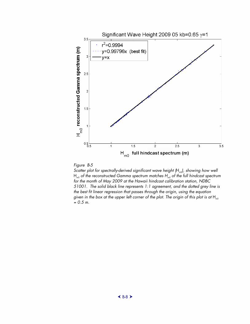
B-8

Figure B-5 Scatter plot for spectrally-derived significant wave height (Hm0), showing how well Hm0 of the reconstructed Gamma spectrum matches Hm0 of the full hindcast spectrum for the month of May 2009 at the Hawaii hindcast calibration station, NDBC 51001. The solid black line represents 1:1 agreement, and the dotted grey line is the best fit linear regression that passes through the origin, using the equation given in the box at the upper left corner of the plot. The origin of this plot is at Hm0 = 0.5 m.

B-9

Figure B-6 Scatter plot for spectrally-derived wave energy period (Te), showing how well Te of the reconstructed Gamma spectrum matches Te of the full hindcast spectrum for the month of May 2009 at the Hawaii hindcast calibration station, NDBC 51001. The solid black line represents 1:1 agreement, and the dotted grey line is the best fit linear regression that passes through the origin, using the equation given in the box at the upper left corner of the plot. The origin of this plot is at Te = 6 sec. The wider scatter of Te compared with Hm0 and P0 suggests that the quotient of m-1 divided by m0 is more sensitive to wave spectral shape than is either spectral moment by itself.

B-10

Figure B-7 Scatter plot for spectrally-derived deep-water wave power density (P0), showing how well P0 of the reconstructed Gamma spectrum matches P0 of the full hindcast spectrum for the month of May 2009 at the Hawaii hindcast calibration station, NDBC 51001. The solid black line represents 1:1 agreement, and the dotted grey line is the best fit linear regression that passes through the origin, using the equation given in the box at the upper left corner of the plot. The origin of this plot is at P0 = 0 kW/m.

B-11

Figure B-8 Plot of r-squared values for 51 months showing fit of Hm0 from reconstructed spectra to Hm0 of full hindcast spectra at Hawaii calibration station (NDBC 51001).

Figure B-9 Plot of r-squared values for 51 months showing fit of Te from reconstructed spectra to Hm0 of full hindcast spectra at Hawaii calibration station (NDBC 51001).

B-12

Figure B-10 Plot of r-Squared Values for 51 Months Showing Fit of P0 from Reconstructed Spectra to P0 of Full Hindcast Spectra at Hawaii Calibration Station (NDBC 51001).

Example plots of the full hindcast non-directional wave spectrum and the “built up” spectrum reconstructed using the Gamma spectral formulation and calibrated spectral shape parameters for May 2009 are given in Figures B-11 through B-18 for the following eight cases (where the reference time zone is “z” for Greenwich Mean Time):

Case A1: 80% of total sea state energy is forced by local winds, May 17, 2009, 2100z

Case A2: 70% of total sea state energy is forced by local winds, May 18, 2009, 0300z

Case B: 65% of total sea state energy is forced by local winds, May 23, 2009, 0300z

Case C: 33% of total sea state energy is forced by local winds, May 18, 2009, 1800z

Case D: 10% of total sea state energy is forced by local winds, May 1, 2009, 0000z

Case E: No local wind forcing, three (3) swell partitions, May 4, 2009, 0600z

B-13

Case F: No local wind forcing, eleven (11) swell partitions, May 11, 2009, 0600z

Case G: No local wind forcing, eleven (9) swell partitions, May 16, 2009, 1500z

Beneath each of the spectral plots for Cases A through F in Figures B-11 through B-16, the listing of Wavewatch III hindcast sea state parameters is given for all partitions. These listings are in the following format:

B-14

Figure B-11 Case A1: 80% of Total Sea State Energy is Forced by Local Winds.

B-15

Figure B-12 Case A2: 70% of total sea state energy is forced by local winds. Note that in this sea state there are two partitions with significant wind forcing (1 and 2).

B-16

Figure B-13 Case B: 65% of Total Sea State Energy is Forced by Local Winds. Note That in Partition 1, the Local Wind Sea Has 32% Swell Content.

B-17

Figure B-14 Case C: 33% of Total Sea State Energy is Forced by Local Winds. Note That in This Sea State There Are Two Partitions with Significant Wind Forcing (1 and 2).

B-18

Figure B-15 Case D: 10% of Total Sea State Energy is Forced by Local Winds.

B-19

Figure B-16 Case E: No Local Wind Forcing, with Three Swell Partitions.

B-20

Figure B-17 Case F: No Local Wind Forcing, with Eleven (11) Swell Partitions, Which is the Largest Number of Swell Trains Hindcast at This Particular Grid Point in May 2009.

B-21

Figure B-18 Case G: No Local Wind Forcing, with Nine (9) Swell Partitions.

C-1

Appendix C: NDBC Measurement Stations and NOAA Full Hindcast Stations

NDBC measurement stations were variously used for four purposes, which are identified in the region-by-region listing below. The four purposes are:

TYPICALNESS STUDY – Determining how well the 4½-year period from February 2005 through July 2009 represents the 12½-year wave climate from February 1997 through July 2009. This is a measurement-to-measurement comparison.

CALIBRATION – Adjusting spectral shape parameters for the Gamma spectrum to obtain best fit (least root-mean-square error in S(f)/f differences) between the NOAA full hindcast spectrum at the co-located NDBC station and the reconstructed spectrum from the NOAA multi-partition hindcast sea state parameters at the nearest grid point. This is a hindcast-to-hindcast comparison.

VALIDATION – Determining how well the annual and monthly wave resource statistics developed from the calibrated hindcast match the measured wave resource statistics. This is a measurement-to-calibrated-hindcast comparison.

DIRECTIONAL FLUX ANALYSIS – Quantifying the effect of using normally directed wave energy flux for wave energy resource estimation, we calculated the directional flux distribution at 17 NDBC full-directional-hindcast stations in four regions that represent the variety of energetic US wave climates.

Within the 15 regions listed in this appendix, a complete set of NDBC measurement stations has been identified for 12 of them. Validation stations could not be identified for the Bering Sea and the two Puerto Rico regions (Atlantic side and Caribbean side).

C-2

Hawaii NDBC Station 51001 - NW HAWAII 170 NM West Northwest of Kauai Island 23.445 N 162.279 W (23°26'42" N 162°16'43" W) Water depth: 3430 m www.ndbc.noaa.gov/station_page.php?station=51001 TYPICALNESS STUDY CALIBRATION NEAREST GRID POINT 23.500 N, 197.833 W Water depth: 3739 m NDBC Station 51201 - Waimea Bay, HI (CDIP 106) 21.673 N 158.116 W (21°40'22" N 158°6'57" W) Water depth: 198 m www.ndbc.noaa.gov/station_page.php?station=51201 VALIDATION NEAREST GRID POINT 21.667 N, 158.133 W Water depth: 434 m NDBC Station 51202 - Mokapu Point, HI (CDIP 098) 21.417 N 157.668 W (21°25'1" N 157°40'4" W) Water depth: 100 m www.ndbc.noaa.gov/station_page.php?station=51202 VALIDATION NEAREST GRID POINT 21.400 N, 157.667 W Water depth: 128 m Bering Sea NDBC Station 46035 - BERING SEA 310 NM North of Adak, AK 57.067 N 177.750 W (57°4'0" N 177°45'0" W) Water depth: 3658 m www.ndbc.noaa.gov/station_page.php?station=46035 TYPICALNESS STUDY CALIBRATION NEAREST GRID POINT 57.0 N, 177.5 W Water depth: 3679 m

There are no long-term measurement stations in the Bering Sea, and so a typicalness evaluation cannot be done for this region.

http://www.ndbc.noaa.gov/station_page.php?station=51001�




C-3

Aleutian Islands, Pacific side NDBC Station 46071 - Western Aleutians 51.155 N 179.001 E (51°9'17" N 179°0'2" E) Water depth: 1373 m www.ndbc.noaa.gov/station_page.php?station=46071 CALIBRATION NEAREST GRID POINT 51.133 N, 181.0 W Water depth: 1942 m NDBC Station 46072 - Central Aleutians 230NM Southwest of Dutch Harbor 51.625 N 172.167 W (51°37'30" N 172°10'0" W) Water depth: 3641 m www.ndbc.noaa.gov/station_page.php?station=46072 VALIDATION NDBC Station 46075 - Shumagin Islands, AK 53.926 N 160.806 W (53°55'32" N 160°48'23" W) Water depth: 2345 m www.ndbc.noaa.gov/station_page.php?station=46075 VALIDATION Gulf of Alaska West NDBC Station 46078 - Albatross Banks AK 56.074 N 152.572 W (56°4'25" N 152°34'20" W) Water depth: 3405 m www.ndbc.noaa.gov/station_page.php?station=46078 CALIBRATION NDBC Station 46061 - Seal Rocks 55NM South of Valdez, AK 60.218 N 146.825 W (60°13'4" N 146°49'30" W) Water depth: 205 m www.ndbc.noaa.gov/station_page.php?station=46061 TYPICALNESS STUDY VALIDATION NDBC Station 46072 - Central Aleutians 230NM Southwest of Dutch Harbor 51.625 N 172.167 W (51°37'30" N 172°10'0" W) Water depth: 3641 m www.ndbc.noaa.gov/station_page.php?station=46072 VALIDATION







C-4

NDBC Station 46075 - Shumagin Islands, AK 53.926 N 160.806 W (53°55'32" N 160°48'23" W) Water depth: 2345 m www.ndbc.noaa.gov/station_page.php?station=46075 VALIDATION NDBC Station 46080 - Northwest Gulf 57NM East of Kodiak, AK 58.035 N 149.994 W (58°2'6" N 149°59'38" W) Water depth: 310 m www.ndbc.noaa.gov/station_page.php?station=46080 VALIDATION Gulf of Alaska East NDBC Station 46084 - Cape Edgecumbe Buoy AK 56.625 N 136.148 W (56°37'30" N 136°8'54" W) Water depth: 1406 m www.ndbc.noaa.gov/station_page.php?station=46084 CALIBRATION NDBC Station 46001 - GULF OF AK 175NM South East of Kodiak, AK 56.300 N 148.021 W (56°17'59" N 148°1'16" W) Water depth: 4206 m www.ndbc.noaa.gov/station_page.php?station=46001 TYPICALNESS STUDY NDBC Station 46082 - Cape Suckling 84NM Southeast of Cordova, AK 59.688 N 143.399 W (59°41'17" N 143°23'56" W) Water depth: 135 m www.ndbc.noaa.gov/station_page.php?station=46082 VALIDATION NDBC Station 46083 - Fairweather Grounds 92NM Southeast of Yakutat, AK 58.243 N 137.993 W (58°14'33" N 137°59'36" W) Water depth: 136 m www.ndbc.noaa.gov/station_page.php?station=46083 VALIDATION Pacific Northwest (WA, OR, and CA north of Cape Mendocino) NDBC Station 46089 - TILAMOOK - 85 NM WNW of Tillamook, OR 45.908 N 125.760 W (45°54'28" N 125°45'37" W) Water depth: 2230 m www.ndbc.noaa.gov/station_page.php?station=46089 CALIBRATION








C-5

NDBC Station 46041 - CAPE ELIZABETH- 45NM Northwest of Aberdeen, WA 47.353 N 124.731 W (47°21'10" N 124°43'50" W) Water depth: 132 m www.ndbc.noaa.gov/station_page.php?station=46041 TYPICALNESS STUDY VALIDATION NDBC Station 46050 - STONEWALL BANKS - 20NM West of Newport, OR 44.641 N 124.500 W (44°38'28" N 124°29'59" W) Water depth: 123 m www.ndbc.noaa.gov/station_page.php?station=46050 TYPICALNESS STUDY VALIDATION NDBC Station 46022 - EEL RIVER - 17NM West-Southwest of Eureka, CA 40.749 N 124.577 W (40°44'58" N 124°34'38" W) Water depth: 631 m www.ndbc.noaa.gov/station_page.php?station=46022 TYPICALNESS STUDY VALIDATION NDBC Station 46211 - Grays Harbor, WA (CDIP 036) 46.857 N 124.244 W (46°51'24" N 124°14'40" W) Water depth: 38 m www.ndbc.noaa.gov/station_page.php?station=46211 VALIDATION NDBC Station 46229 - UMPQUA OFFSHORE, OR (CDIP 139) 43.769 N 124.551 W (43°46'10" N 124°33'2" W) Water depth: 187 m www.ndbc.noaa.gov/station_page.php?station=46229 VALIDATION NDBC Station 46027 - ST GEORGES - 8NM West Northwest of Crescent City, CA 41.850 N 124.381 W (41°51'1" N 124°22'52" W) Water depth: 47.9 m www.ndbc.noaa.gov/station_page.php?station=46027 VALIDATION







C-6

Central California (between Cape Mendocino and Point Arguello) NDBC Station 46042 - MONTEREY - 27NM West of Monterey Bay, CA 36.789 N 122.404 W (36°47'19" N 122°24'15" W) Water depth: 1574 m www.ndbc.noaa.gov/station_page.php?station=46042 CALIBRATION NDBC Station 46013 - Bodega Bay - 48NM North Northwest of San Francisco, CA 38.242 N 123.301 W (38°14'31" N 123°18'2" W) Water depth: 116 m www.ndbc.noaa.gov/station_page.php?station=46013 TYPICALNESS STUDY VALIDATION NDBC Station 46028 - CAPE SAN MARTIN - 55NM West Northwest of Morro Bay, CA 35.741 N 121.884 W (35°44'29" N 121°53'3" W) Water depth: 1158 m www.ndbc.noaa.gov/station_page.php?station=46028 TYPICALNESS STUDY VALIDATION NDBC Station 46014 - PT ARENA - 19NM North of Point Arena, CA 39.196 N 123.969 W (39°11'45" N 123°58'10" W) Water depth: 274 m www.ndbc.noaa.gov/station_page.php?station=46014 VALIDATION NDBC Station 46026 - SAN FRANCISCO - 18NM West of San Francisco, CA 37.759 N 122.833 W (37°45'32" N 122°50'0" W) Water depth: 52.1 m www.ndbc.noaa.gov/station_page.php?station=46026 VALIDATION NDBC Station 46012 - HALF MOON BAY - 24NM South Southwest of San Francisco, CA 7.361 N 122.881 W (37°21'39" N 122°52'53" W) Water depth: 213 m www.ndbc.noaa.gov/station_page.php?station=46012 VALIDATION







C-7

NDBC Station 46023 - PT ARGUELLO - 17NM West Northwest of Point Arguello, CA 34.714 N 120.967 W (34°42'50" N 120°58'0" W) Water depth: 384 m www.ndbc.noaa.gov/station_page.php?station=46023 VALIDATION Southern California (south of Point Arguello) NDBC Station 46047 - TANNER BANKS - 121NM West of San Diego, CA 32.433 N 119.533 W (32°26'0" N 119°31'59" W) Water depth: 1394 m www.ndbc.noaa.gov/station_page.php?station=46047 CALIBRATION NDBC Station 46054 - SANTA BARBARA W 38 NM West of Santa Barbara, CA 34.274 N 120.459 W (34°16'28" N 120°27'34" W) Water depth: 460 m www.ndbc.noaa.gov/station_page.php?station=46054 TYPICALNESS STUDY VALIDATION NDBC Station 46025 - Santa Monica Basin - 33NM West Southwest of Santa Monica, CA 33.739 N 119.056 W (33°44'20" N 119°3'20" W) Water depth: 882 m www.ndbc.noaa.gov/station_page.php?station=46025 TYPICALNESS STUDY VALIDATION NDBC Station 46217 - Anacapa Passage, CA (CDIP 111) 34.167 N 119.435 W (34°10'2" N 119°26'5" W) Water depth: 110 m www.ndbc.noaa.gov/station_page.php?station=46217 VALIDATION NDBC Station 46222 - San Pedro, CA (CDIP 092) 33.618 N 118.317 W (33°37'4" N 118°19'1" W) Water depth: 457 m www.ndbc.noaa.gov/station_page.php?station=46222 VALIDATION







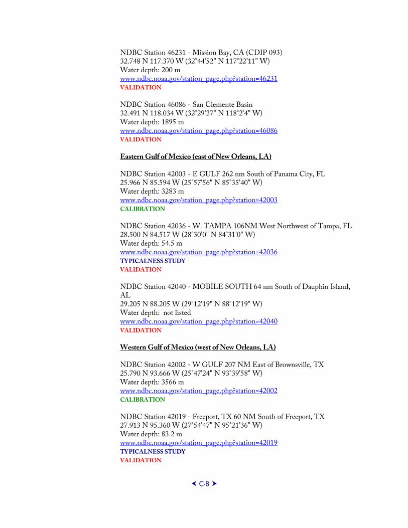
C-8

NDBC Station 46231 - Mission Bay, CA (CDIP 093) 32.748 N 117.370 W (32°44'52" N 117°22'11" W) Water depth: 200 m www.ndbc.noaa.gov/station_page.php?station=46231 VALIDATION NDBC Station 46086 - San Clemente Basin 32.491 N 118.034 W (32°29'27" N 118°2'4" W) Water depth: 1895 m www.ndbc.noaa.gov/station_page.php?station=46086 VALIDATION Eastern Gulf of Mexico (east of New Orleans, LA) NDBC Station 42003 - E GULF 262 nm South of Panama City, FL 25.966 N 85.594 W (25°57'56" N 85°35'40" W) Water depth: 3283 m www.ndbc.noaa.gov/station_page.php?station=42003 CALIBRATION NDBC Station 42036 - W. TAMPA 106NM West Northwest of Tampa, FL 28.500 N 84.517 W (28°30'0" N 84°31'0" W) Water depth: 54.5 m www.ndbc.noaa.gov/station_page.php?station=42036 TYPICALNESS STUDY VALIDATION NDBC Station 42040 - MOBILE SOUTH 64 nm South of Dauphin Island, AL 29.205 N 88.205 W (29°12'19" N 88°12'19" W) Water depth: not listed www.ndbc.noaa.gov/station_page.php?station=42040 VALIDATION Western Gulf of Mexico (west of New Orleans, LA) NDBC Station 42002 - W GULF 207 NM East of Brownsville, TX 25.790 N 93.666 W (25°47'24" N 93°39'58" W) Water depth: 3566 m www.ndbc.noaa.gov/station_page.php?station=42002 CALIBRATION NDBC Station 42019 - Freeport, TX 60 NM South of Freeport, TX 27.913 N 95.360 W (27°54'47" N 95°21'36" W) Water depth: 83.2 m www.ndbc.noaa.gov/station_page.php?station=42019 TYPICALNESS STUDY VALIDATION








C-9

NDBC Station 42020 - Corpus Christi - 50NM Southeast of Corpus Christi, TX 26.966 N 96.695 W (26°57'59" N 96°41'42" W) Water depth: 88.1 m www.ndbc.noaa.gov/station_page.php?station=42020 VALIDATION Southeast Atlantic (from Savannah, GA to Key West, FL) NDBC Station 41010 - CANAVERAL EAST 120NM East of Cape Canaveral 28.906 N 78.471 W (28°54'22" N 78°28'16" W) Water depth: 873 m www.ndbc.noaa.gov/station_page.php?station=41010 CALIBRATION NDBC Station 41009 - CANAVERAL 20 NM East of Cape Canaveral, FL 28.519 N 80.166 W (28°31'9" N 80°9'59" W) Water depth: 44.2 m www.ndbc.noaa.gov/station_page.php?station=41009 TYPICALNESS STUDY VALIDATION NDBC Station 42080 - Offshore Sand Key, FL 24.396 N 81.934 W (24°23'44" N 81°56'2" W) Water depth: 120 m www.ndbc.noaa.gov/station_page.php?station=42080 TYPICALNESS STUDY VALIDATION NDBC Station 41008 - GRAYS REEF - 40 NM Southeast of Savannah, GA 31.402 N 80.869 W (31°24'9" N 80°52'9" W) Water depth: 18.3 m www.ndbc.noaa.gov/station_page.php?station=41008 VALIDATION NDBC Station 41012 - St. Augustine - 40NM ENE of St Augustine, FL 30.041 N 80.533 W (30°2'29" N 80°32'0" W) Water depth: 37.2 m www.ndbc.noaa.gov/station_page.php?station=41012 VALIDATION







C-10

Mid-Atlantic (between Hudson Canyon and Savannah, GA) NDBC Station 41001 - 150 NM East of Cape HATTERAS 34.704 N 72.734 W (34°42'13" N 72°44'2" W) Water depth: 4426 m www.ndbc.noaa.gov/station_page.php?station=41001 CALIBRATION NDBC Station 44014 - VIRGINIA BEACH 64 NM East of Virginia Beach, VA 36.611 N 74.836 W (36°36'40" N 74°50'11" W) Water depth: 47.5 m www.ndbc.noaa.gov/station_page.php?station=44014 TYPICALNESS STUDY VALIDATION NDBC Station 41004 - EDISTO - 41 NM Southeast of Charleston, SC 32.501 N 79.099 W (32°30'2" N 79°5'58" W) Water depth: 38.4 m www.ndbc.noaa.gov/station_page.php?station=41004 TYPICALNESS STUDY VALIDATION NDBC Station 44009 - DELAWARE BAY 26 NM Southeast of Cape May, NJ 38.464 N 74.702 W (38°27'49" N 74°42'7" W) Water depth: 28 m www.ndbc.noaa.gov/station_page.php?station=44009 VALIDATION NDBC Station 41025 - Diamond Shoals 35.006 N 75.402 W (35°0'22" N 75°24'7" W) Water depth: 68.3 m www.ndbc.noaa.gov/station_page.php?station=41025 VALIDATION NDBC Station 41013 - Frying Pan Shoals, NC Buoy 33.436 N 77.743 W (33°26'11" N 77°44'35" W) Water depth: 23.5 m www.ndbc.noaa.gov/station_page.php?station=41013 VALIDATION







C-11

Northeast Atlantic (north of Hudson River Shelf Valley) NDBC Station 44011 - GEORGES BANK 170 NM East of Hyannis, MA 41.111 N 66.580 W (41°6'41" N 66°34'47" W) Water depth: 88.4 m www.ndbc.noaa.gov/station_page.php?station=46047 CALIBRATION NDBC Station 44005 - GULF OF MAINE 78 NM EAST OF PORTSMOUTH,NH 43.189 N 69.140 W (43°11'22" N 69°8'23" W) Water depth: 201 m www.ndbc.noaa.gov/station_page.php?station=44005 TYPICALNESS STUDY VALIDATION NDBC Station 44008 - NANTUCKET 54NM Southeast of Nantucket 40.503 N 69.247 W (40°30'9" N 69°14'48" W) Water depth: 59.1 m www.ndbc.noaa.gov/station_page.php?station=44008 TYPICALNESS STUDY VALIDATION NDBC Station 44027 - Jonesport, Maine 44.273 N 67.314 W (44°16'21" N 67°18'51" W) Water depth: 180 m www.ndbc.noaa.gov/station_page.php?station=44027 VALIDATION NDBC Station 44018 - SE Cape Cod 30NM East of Nantucket, MA 41.255 N 69.305 W (41°15'19" N 69°18'18" W) Water depth: 63.7 m www.ndbc.noaa.gov/station_page.php?station=44018 VALIDATION NDBC Station 44017 - 23 Nautical Miles Southwest of Montauk Point, NY 40.691 N 72.046 W (40°41'27" N 72°2'47" W) Water depth: 46 m www.ndbc.noaa.gov/station_page.php?station=44017 VALIDATION NDBC Station 44025 - LONG ISLAND 33 NM South of Islip, NY 40.250 N 73.166 W (40°15'1" N 73°9'59" W) Water depth: 36.3 m www.ndbc.noaa.gov/station_page.php?station=44025 VALIDATION








C-12

Puerto Rico, Atlantic Side NDBC Station 41043 - South Western Atlantic 20.989 N 65.014 W (20°59'20" N 65°0'49" W) Water depth: 5259 m www.ndbc.noaa.gov/station_page.php?station=41043 CALIBRATION – ATLANTIC WAVE CLIMATE Puerto Rico, Caribbean Side NDBC Station 42059 - Eastern Caribbean 15.006 N 67.496 W (15°0'20" N 67°29'44" W) Water depth: 4900 m www.ndbc.noaa.gov/station_page.php?station=42059 CALIBRATION – CARIBBEAN WAVE CLIMATE

There are no long-term measurement stations near Puerto Rico, and so a typicalness study cannot be done for this territory.



D-1

Appendix D: Validation Results

D-2

Table D-1 Comparison of Model vs. Measured Wave Power Density (WPD) by Buoy

Buoy Region Avg WPD Model (kW/m)

Avg WPD Buoy

(kW/m)

Ratio Difference (kW/m)

46061 AK 13.40 15.46 0.867 -2.06 46072 AK 45.32 52.31 0.866 -6.99 46075 AK 35.78 43.26 0.827 -7.48 46080 AK 23.54 33.24 0.708 -9.70 46082 AK 27.42 34.97 0.784 -7.55 46083 AK 31.32 35.22 0.889 -3.90 46012 CC 32.78 32.32 1.014 0.46 46013 CC 33.50 27.62 1.213 5.88 46014 CC 37.40 31.50 1.187 5.90 46023 CC 31.70 29.67 1.068 2.03 46026 CC 20.04 20.79 0.964 -0.75 46028 CC 33.24 29.89 1.112 3.35 42036 EM 2.96 4.56 0.649 -1.60 42040 EM 4.80 5.88 0.816 -1.08 51201 HI 16.10 14.28 1.127 1.82 51202 HI 15.60 14.67 1.063 0.93 41013 MA 6.88 7.30 0.942 -0.42 41025 MA 9.38 10.34 0.907 -0.96 44009 MA 4.70 6.76 0.695 -2.06 44014 MA 8.44 10.10 0.836 -1.66 44017 MA 6.88 8.18 0.841 -1.30 44025 MA 5.82 7.70 0.756 -1.88 44005 NE 6.46 10.98 0.588 -4.52 44008 NE 13.78 17.57 0.784 -3.79 44018 NE 10.28 11.46 0.897 -1.18 44027 NE 5.60 8.25 0.679 -2.65 46022 PN 39.76 33.96 1.171 5.80 46027 PN 33.68 28.29 1.191 5.39 46041 PN 39.02 33.31 1.171 5.71 46050 PN 39.26 35.37 1.110 3.89 46211 PN 32.20 27.07 1.190 5.13 46229 PN 39.18 33.39 1.173 5.79 41004 SA 6.82 7.15 0.954 -0.33 41008 SA 3.08 3.58 0.860 -0.50 41009 SA 7.24 6.75 1.073 0.49 41012 SA 6.66 6.30 1.057 0.36 46025 SC 4.82 6.04 0.798 -1.22 46054 SC 25.00 21.47 1.164 3.53 46086 SC 13.20 13.12 1.006 0.08 46217 SC 3.20 5.28 0.606 -2.08 46222 SC 2.60 4.74 0.549 -2.14 46231 SC 4.80 6.65 0.722 -1.85 42019 WM 5.10 6.52 0.782 -1.42 42020 WM 5.68 7.68 0.740 -2.00

D-3

Table D-2 Comparison of Buoy Wave Power Density (WPD, kW/m) Values with Nearest Five Grid Points

Region Buoy Avg WPD

Model

Avg WPD Buoy

Avg Ratio

Min Ratio

Max Ratio

Avg Diff

Min Diff

Max Diff

AK 46061 12.20 15.46 0.789 0.692 1.125 -3.26 -11.33 0.61

AK 46061 13.80 15.46 0.893 0.766 1.268 -1.66 -8.63 1.31

AK 46061 14.20 15.46 0.918 0.787 1.309 -1.26 -7.83 1.51

AK 46061 10.50 15.46 0.679 0.600 0.961 -4.96 -14.73 -0.19

AK 46061 16.30 15.46 1.054 0.896 1.493 0.84 -3.83 2.67

AK 46072 45.20 52.31 0.864 0.764 1.086 -7.11 -15.04 0.97

AK 46072 44.80 52.31 0.856 0.755 1.077 -7.51 -15.64 0.87

AK 46072 45.70 52.31 0.874 0.778 1.095 -6.61 -14.14 1.07

AK 46072 45.20 52.31 0.864 0.769 1.086 -7.11 -14.74 0.97

AK 46072 45.70 52.31 0.874 0.772 1.095 -6.61 -14.54 1.07

AK 46075 35.90 43.26 0.830 0.717 1.015 -7.36 -16.66 0.15

AK 46075 36.60 43.26 0.846 0.743 1.034 -6.66 -15.56 0.35

AK 46075 35.50 43.26 0.821 0.708 1.005 -7.76 -17.26 0.05

AK 46075 35.70 43.26 0.825 0.717 1.015 -7.56 -16.86 0.15

AK 46075 35.20 43.26 0.814 0.701 1.005 -8.06 -17.66 0.05

AK 46080 23.60 33.24 0.710 0.453 1.369 -9.64 -31.85 4.12

AK 46080 23.90 33.24 0.719 0.460 1.369 -9.34 -31.45 4.12

AK 46080 23.30 33.24 0.701 0.448 1.360 -9.94 -32.15 4.02

AK 46080 23.30 33.24 0.701 0.446 1.360 -9.94 -32.25 4.02

AK 46080 23.60 33.24 0.710 0.453 1.360 -9.64 -31.85 4.02

AK 46082 27.80 34.97 0.795 0.689 1.157 -7.17 -25.48 2.28

AK 46082 26.90 34.97 0.769 0.659 1.129 -8.07 -27.18 1.88

AK 46082 27.80 34.97 0.795 0.691 1.157 -7.17 -25.28 2.28

AK 46082 27.70 34.97 0.792 0.685 1.164 -7.27 -25.78 2.38

AK 46082 26.90 34.97 0.769 0.668 1.123 -8.07 -27.08 1.78

AK 46083 31.00 35.22 0.880 0.696 1.061 -4.22 -19.68 3.09

AK 46083 31.50 35.22 0.894 0.708 1.077 -3.72 -18.88 3.89

AK 46083 31.60 35.22 0.897 0.711 1.079 -3.62 -18.68 3.99

AK 46083 32.10 35.22 0.911 0.724 1.095 -3.12 -17.88 5.04

AK 46083 30.40 35.22 0.863 0.680 1.043 -4.82 -20.68 2.09

CC 46013 33.40 27.62 1.209 1.058 1.290 5.78 1.09 12.53

CC 46013 31.30 27.62 1.133 0.978 1.209 3.68 -0.41 8.43

CC 46013 34.70 27.62 1.256 1.127 1.331 7.08 2.14 14.43

CC 46013 32.80 27.62 1.188 1.058 1.261 5.18 1.09 10.73

CC 46013 35.30 27.62 1.278 1.132 1.357 7.68 2.34 16.03

CC 46028 33.30 29.89 1.114 1.002 1.197 3.41 0.05 8.90

D-4

Table D-2 (continued) Comparison of Buoy Wave Power Density (WPD, kW/m) Values with Nearest Five Grid Points

Region Buoy Avg WPD

Model

Avg WPD Buoy

Avg Ratio

Min Ratio

Max Ratio

Avg Diff

Min Diff

Max Diff

CC 46028 33.80 29.89 1.131 1.029 1.210 3.91 0.58 9.50

CC 46028 32.90 29.89 1.101 0.980 1.190 3.01 -0.45 8.60

CC 46028 32.70 29.89 1.094 0.971 1.184 2.81 -0.65 8.30

CC 46028 33.50 29.89 1.121 1.007 1.204 3.61 0.15 9.20

CC 46014 37.80 31.50 1.200 0.982 1.346 6.30 -0.30 16.35

CC 46014 36.40 31.50 1.156 0.910 1.310 4.90 -1.50 14.65

CC 46014 38.20 31.50 1.213 1.012 1.352 6.70 0.20 16.65

CC 46014 37.10 31.50 1.178 0.952 1.321 5.60 -0.80 15.15

CC 46014 37.50 31.50 1.190 0.952 1.344 6.00 -0.80 16.25

CC 46026 22.80 20.79 1.097 0.960 1.163 2.01 -0.58 5.35

CC 46026 20.80 20.79 1.000 0.878 1.075 0.01 -1.78 2.45

CC 46026 17.60 20.79 0.847 0.761 0.907 -3.19 -5.55 -1.20

CC 46026 20.30 20.79 0.976 0.885 1.035 -0.49 -1.68 1.15

CC 46026 18.70 20.79 0.899 0.761 0.986 -2.09 -3.48 -0.45

CC 46012 33.20 32.32 1.027 0.914 1.150 0.88 -2.45 7.16

CC 46012 31.30 32.32 0.968 0.856 1.089 -1.02 -4.55 4.26

CC 46012 34.90 32.32 1.080 0.977 1.201 2.58 -0.75 9.36

CC 46012 33.40 32.32 1.033 0.925 1.156 1.08 -2.35 7.46

CC 46012 31.10 32.32 0.962 0.851 1.079 -1.22 -4.75 3.76

CC 46023 31.70 29.67 1.068 0.901 1.151 2.03 -3.15 6.60

CC 46023 31.00 29.67 1.045 0.883 1.135 1.33 -3.75 5.90

CC 46023 32.10 29.67 1.082 0.914 1.160 2.43 -2.75 7.00

CC 46023 31.50 29.67 1.062 0.898 1.144 1.83 -3.25 6.30

CC 46023 32.20 29.67 1.085 0.920 1.167 2.53 -2.55 7.30

EM 42036 3.10 4.56 0.680 0.560 2.442 -1.46 -2.88 1.24

EM 42036 2.90 4.56 0.636 0.522 2.326 -1.66 -3.18 1.14

EM 42036 3.10 4.56 0.680 0.560 2.442 -1.46 -2.80 1.24

EM 42036 2.80 4.56 0.614 0.509 2.209 -1.76 -3.28 1.04

EM 42036 2.90 4.56 0.636 0.539 2.326 -1.66 -3.08 1.14

EM 42040 4.80 5.88 0.816 0.541 1.782 -1.08 -2.27 0.79

EM 42040 4.80 5.88 0.816 0.541 1.782 -1.08 -2.17 0.79

EM 42040 4.70 5.88 0.799 0.541 1.782 -1.18 -2.57 0.79

EM 42040 4.80 5.88 0.816 0.541 1.782 -1.08 -2.27 0.79

EM 42040 4.90 5.88 0.833 0.579 1.782 -0.98 -2.07 0.79

HI 51201 14.40 14.28 1.008 0.796 1.383 0.12 -4.85 8.67

HI 51201 13.80 14.28 0.966 0.467 1.436 -0.48 -5.05 9.87

HI 51201 20.70 14.28 1.450 1.107 1.874 6.42 2.26 19.77

D-5


Region Buoy Avg WPD

Model

Avg WPD Buoy

Avg Ratio

Min Ratio

Max Ratio

Avg Diff

Min Diff

Max Diff

HI 51201 9.90 14.28 0.693 0.302 1.047 -4.38 -10.25 1.07

HI 51201 21.70 14.28 1.520 1.162 1.958 7.42 2.46 21.67

HI 51202 12.70 14.67 0.866 0.766 0.938 -1.97 -3.55 -1.10

HI 51202 16.50 14.67 1.125 0.873 1.409 1.83 -1.11 8.07

HI 51202 16.50 14.67 1.125 0.907 1.374 1.83 -0.81 7.37

HI 51202 12.40 14.67 0.845 0.677 0.978 -2.27 -3.55 -0.43

HI 51202 19.90 14.67 1.357 0.964 1.804 5.23 -0.31 15.87

MA 44017 7.00 8.18 0.856 0.663 1.350 -1.18 -4.21 1.14

MA 44017 7.20 8.18 0.880 0.687 1.380 -0.98 -3.91 1.24

MA 44017 6.60 8.18 0.807 0.622 1.288 -1.58 -4.71 0.94

MA 44017 6.80 8.18 0.831 0.647 1.319 -1.38 -4.41 1.04

MA 44017 6.80 8.18 0.831 0.639 1.319 -1.38 -4.41 1.04

MA 44025 5.80 7.70 0.753 0.553 1.126 -1.90 -4.52 0.87

MA 44025 5.50 7.70 0.714 0.514 1.097 -2.20 -4.92 0.67

MA 44025 6.00 7.70 0.779 0.583 1.183 -1.70 -4.22 1.27

MA 44025 5.80 7.70 0.753 0.553 1.140 -1.90 -4.52 0.97

MA 44025 6.00 7.70 0.779 0.583 1.154 -1.70 -4.22 1.07

MA 44014 8.40 10.10 0.832 0.637 0.995 -1.70 -3.94 -0.02

MA 44014 8.90 10.10 0.881 0.683 1.065 -1.20 -3.44 0.40

MA 44014 8.20 10.10 0.812 0.618 0.972 -1.90 -4.14 -0.12

MA 44014 8.70 10.10 0.861 0.673 1.042 -1.40 -3.54 0.20

MA 44014 8.00 10.10 0.792 0.590 0.949 -2.10 -4.44 -0.22

MA 44009 4.50 6.76 0.666 0.461 0.888 -2.26 -3.74 -0.34

MA 44009 4.90 6.76 0.725 0.519 0.987 -1.86 -3.34 -0.04

MA 44009 4.70 6.76 0.695 0.476 0.921 -2.06 -3.64 -0.24

MA 44009 5.10 6.76 0.754 0.533 1.020 -1.66 -3.24 0.06

MA 44009 4.30 6.76 0.636 0.432 0.855 -2.46 -3.94 -0.44

MA 41025 9.50 10.34 0.919 0.767 1.160 -0.84 -3.32 0.77

MA 41025 8.30 10.34 0.803 0.668 1.086 -2.04 -4.92 0.35

MA 41025 10.50 10.34 1.015 0.864 1.220 0.16 -2.02 1.93

MA 41025 8.10 10.34 0.783 0.661 1.037 -2.24 -5.02 0.17

MA 41025 10.50 10.34 1.015 0.850 1.220 0.16 -2.22 2.03

MA 41013 6.80 7.30 0.932 0.745 1.138 -0.50 -2.50 1.44

MA 41013 7.20 7.30 0.986 0.786 1.205 -0.10 -2.10 2.14

MA 41013 6.50 7.30 0.890 0.714 1.080 -0.80 -2.80 0.84

MA 41013 6.90 7.30 0.945 0.765 1.168 -0.40 -2.30 1.74

D-6


Region Buoy Avg WPD

Model

Avg WPD Buoy

Avg Ratio

Min Ratio

Max Ratio

Avg Diff

Min Diff

Max Diff

MA 41013 7.00 7.30 0.959 0.776 1.195 -0.30 -2.20 2.04

NE 44005 6.40 10.98 0.583 0.418 0.986 -4.58 -11.14 -0.05

NE 44005 6.30 10.98 0.574 0.402 0.965 -4.68 -11.44 -0.08

NE 44005 6.60 10.98 0.601 0.434 1.014 -4.38 -10.84 0.05

NE 44005 6.60 10.98 0.601 0.434 1.014 -4.38 -10.84 0.05

NE 44005 6.40 10.98 0.583 0.418 0.986 -4.58 -11.14 -0.05

NE 44008 14.00 17.57 0.797 0.679 1.191 -3.57 -9.54 1.06

NE 44008 13.80 17.57 0.785 0.671 1.191 -3.77 -9.94 1.06

NE 44008 13.70 17.57 0.780 0.659 1.173 -3.87 -10.14 0.96

NE 44008 13.90 17.57 0.791 0.671 1.191 -3.67 -9.64 1.06

NE 44008 13.50 17.57 0.768 0.651 1.173 -4.07 -10.54 0.96

NE 44027 5.70 8.25 0.691 0.520 1.127 -2.55 -6.50 0.44

NE 44027 5.80 8.25 0.703 0.535 1.127 -2.45 -6.30 0.44

NE 44027 5.40 8.25 0.655 0.483 1.098 -2.85 -7.10 0.34

NE 44027 5.60 8.25 0.679 0.505 1.127 -2.65 -6.80 0.44

NE 44027 5.50 8.25 0.667 0.498 1.098 -2.75 -6.80 0.34

NE 44018 10.10 11.46 0.881 0.730 1.235 -1.36 -4.74 0.99

NE 44018 10.60 11.46 0.925 0.772 1.283 -0.86 -3.94 1.19

NE 44018 10.40 11.46 0.908 0.754 1.283 -1.06 -4.15 1.19

NE 44018 10.90 11.46 0.951 0.795 1.330 -0.56 -3.45 1.39

NE 44018 9.40 11.46 0.820 0.682 1.164 -2.06 -5.84 0.69

PN 46041 39.70 33.31 1.192 1.034 1.412 6.39 0.32 22.19

PN 46041 39.40 33.31 1.183 1.034 1.401 6.09 0.32 21.59

PN 46041 37.80 33.31 1.135 0.991 1.347 4.49 -0.08 18.69

PN 46041 40.70 33.31 1.222 1.066 1.450 7.39 0.62 24.19

PN 46041 37.50 33.31 1.126 0.981 1.334 4.19 -0.18 17.99

PN 46050 40.40 35.37 1.142 0.976 1.258 5.03 -0.37 17.15

PN 46050 39.20 35.37 1.108 0.951 1.219 3.83 -0.77 13.85

PN 46050 40.10 35.37 1.134 0.976 1.245 4.73 -0.37 16.15

PN 46050 38.50 35.37 1.088 0.951 1.192 3.13 -0.77 11.75

PN 46050 38.10 35.37 1.077 0.931 1.181 2.73 -1.07 11.05

PN 46022 40.00 33.96 1.178 1.071 1.247 6.04 1.27 13.58

PN 46022 39.20 33.96 1.154 1.021 1.233 5.24 0.37 12.78

PN 46022 39.90 33.96 1.175 1.060 1.247 5.94 1.07 13.68

PN 46022 39.10 33.96 1.151 1.015 1.233 5.14 0.27 12.88

PN 46022 40.60 33.96 1.196 1.110 1.263 6.64 1.97 14.18

PN 46211 32.30 27.07 1.193 1.087 1.529 5.23 1.03 10.77

D-7


Region Buoy Avg WPD

Model

Avg WPD Buoy

Avg Ratio

Min Ratio

Max Ratio

Avg Diff

Min Diff

Max Diff

PN 46211 31.20 27.07 1.153 1.015 1.468 4.13 0.17 9.77

PN 46211 33.10 27.07 1.223 1.113 1.568 6.03 1.23 12.27

PN 46211 34.40 27.07 1.271 1.150 1.635 7.33 1.63 14.17

PN 46211 30.00 27.07 1.108 0.997 1.424 2.93 -0.03 7.62

PN 46229 39.00 33.39 1.168 1.045 1.446 5.61 0.41 22.70

PN 46229 39.10 33.39 1.171 1.036 1.448 5.71 0.35 22.80

PN 46229 39.90 33.39 1.195 1.078 1.477 6.51 0.71 24.30

PN 46229 40.00 33.39 1.198 1.078 1.479 6.61 0.71 24.40

PN 46229 37.90 33.39 1.135 1.005 1.405 4.51 0.05 20.60

PN 46027 34.40 28.29 1.216 0.787 1.884 6.11 -2.78 29.80

PN 46027 30.40 28.29 1.075 0.665 1.691 2.11 -4.88 23.30

PN 46027 35.30 28.29 1.248 0.819 1.929 7.01 -2.38 31.30

PN 46027 31.40 28.29 1.110 0.697 1.742 3.11 -4.38 25.00

PN 46027 36.90 28.29 1.304 0.868 2.012 8.61 -1.63 34.10

SA 41004 6.70 7.15 0.937 0.798 1.118 -0.45 -1.98 0.47

SA 41004 6.50 7.15 0.909 0.767 1.092 -0.65 -2.28 0.37

SA 41004 7.10 7.15 0.993 0.849 1.182 -0.05 -1.48 0.59

SA 41004 6.80 7.15 0.951 0.818 1.150 -0.35 -1.78 0.47

SA 41004 7.00 7.15 0.979 0.828 1.150 -0.15 -1.68 0.57

SA 41009 7.50 6.75 1.111 0.922 1.366 0.75 -0.83 2.38

SA 41009 7.00 6.75 1.037 0.865 1.317 0.25 -1.43 1.68

SA 41009 7.40 6.75 1.096 0.913 1.344 0.65 -0.93 2.38

SA 41009 6.80 6.75 1.007 0.837 1.220 0.05 -1.73 1.38

SA 41009 7.50 6.75 1.111 0.922 1.366 0.75 -0.83 2.38

SA 41008 3.10 3.58 0.866 0.702 0.988 -0.48 -1.09 -0.03

SA 41008 2.60 3.58 0.726 0.620 0.864 -0.98 -1.59 -0.33

SA 41008 3.50 3.58 0.978 0.826 1.111 -0.08 -0.49 0.27

SA 41008 2.90 3.58 0.810 0.661 0.947 -0.68 -1.39 -0.13

SA 41008 3.30 3.58 0.922 0.744 1.029 -0.28 -0.79 0.07

SA 41012 6.70 6.30 1.063 0.872 1.360 0.40 -1.54 1.33

SA 41012 6.70 6.30 1.063 0.880 1.360 0.40 -1.44 1.43

SA 41012 6.40 6.30 1.016 0.847 1.316 0.10 -1.84 0.93

SA 41012 7.10 6.30 1.127 0.930 1.447 0.80 -0.84 1.83

SA 41012 6.40 6.30 1.016 0.839 1.316 0.10 -1.94 0.93

SC 46054 25.60 21.47 1.192 0.870 1.883 4.13 -3.33 21.95

SC 46054 21.90 21.47 1.020 0.722 1.666 0.43 -7.13 16.55

D-8


Region Buoy Avg WPD

Model

Avg WPD Buoy

Avg Ratio

Min Ratio

Max Ratio

Avg Diff

Min Diff

Max Diff

SC 46054 21.70 21.47 1.011 0.718 1.610 0.23 -7.23 15.15 SC 46054 28.50 21.47 1.327 0.991 2.048 7.03 -0.23 26.05 SC 46054 27.30 21.47 1.272 0.948 1.976 5.83 -1.33 24.25 SC 46025 4.80 6.04 0.795 0.653 1.013 -1.24 -2.79 0.05 SC 46025 4.70 6.04 0.778 0.653 1.013 -1.34 -3.02 0.05 SC 46025 4.00 6.04 0.662 0.531 0.935 -2.04 -4.42 -0.25 SC 46025 4.90 6.04 0.811 0.673 0.987 -1.14 -2.49 -0.05 SC 46025 5.70 6.04 0.944 0.816 1.117 -0.34 -1.19 0.45 SC 46217 3.00 5.28 0.568 0.375 0.749 -2.28 -3.46 -1.38 SC 46217 3.90 5.28 0.739 0.530 0.967 -1.38 -2.66 -0.24 SC 46217 2.60 5.28 0.492 0.309 0.627 -2.68 -3.86 -1.44 SC 46217 3.10 5.28 0.587 0.419 0.777 -2.18 -3.26 -1.28 SC 46217 3.40 5.28 0.644 0.368 0.886 -1.88 -3.16 -0.84 SC 46222 2.70 4.74 0.570 0.408 0.655 -2.04 -3.47 -1.13 SC 46222 2.70 4.74 0.570 0.457 0.719 -2.04 -3.97 -0.73 SC 46222 2.50 4.74 0.527 0.408 0.612 -2.24 -4.07 -1.03 SC 46222 2.40 4.74 0.506 0.385 0.683 -2.34 -4.77 -0.83 SC 46222 2.70 4.74 0.570 0.372 0.695 -2.04 -3.07 -1.33 SC 46231 5.10 6.65 0.767 0.658 0.973 -1.55 -3.01 -0.09 SC 46231 4.60 6.65 0.692 0.585 0.852 -2.05 -3.61 -0.49 SC 46231 4.70 6.65 0.707 0.603 0.961 -1.95 -3.81 -0.18 SC 46231 4.10 6.65 0.617 0.530 0.790 -2.55 -4.35 -0.69 SC 46231 5.50 6.65 0.827 0.695 1.094 -1.15 -2.81 0.42 SC 46086 14.00 13.12 1.067 0.841 1.290 0.88 -1.85 5.42 SC 46086 13.20 13.12 1.006 0.798 1.215 0.08 -2.35 4.02 SC 46086 12.40 13.12 0.945 0.773 1.124 -0.72 -2.65 2.32 SC 46086 11.60 13.12 0.884 0.730 1.039 -1.52 -3.96 0.72 SC 46086 14.80 13.12 1.128 0.876 1.370 1.68 -1.45 6.92

WM 42019 5.10 6.52 0.782 0.634 0.866 -1.42 -2.61 -0.62 WM 42019 5.00 6.52 0.767 0.634 0.866 -1.52 -2.71 -0.62 WM 42019 5.20 6.52 0.798 0.672 0.887 -1.32 -2.41 -0.52 WM 42019 5.10 6.52 0.782 0.672 0.887 -1.42 -2.51 -0.52 WM 42019 5.10 6.52 0.782 0.634 0.866 -1.42 -2.61 -0.62 WM 42020 5.70 7.68 0.742 0.572 0.840 -1.98 -3.55 -0.43 WM 42020 5.70 7.68 0.742 0.572 0.840 -1.98 -3.65 -0.43 WM 42020 5.60 7.68 0.729 0.558 0.830 -2.08 -3.65 -0.43 WM 42020 5.60 7.68 0.729 0.558 0.830 -2.08 -3.75 -0.43 WM 42020 5.80 7.68 0.755 0.587 0.853 -1.88 -3.45 -0.43

E-1

Appendix E: Results of Typicalness Assessment

Table E-1 shows the difference in wave power density (in kW/m) between the 52-month period and the 12.5-year period. Table values are computed as short-period monthly average minus long-period monthly average. The final column (Avg_52m) shows the average 52-month wave power density in kW/m and is included to distinguish high-energy buoys from lower-energy buoys, the latter of which are shaded in yellow if the annual average wave power density is less than 10 kW/m.

E-2

Table E-1 Difference in Wave Power Density (kW/m) Between 52-month and 12.5-year Periods.

BUOY REG JAN FEB MAR APR MAY JUN JUL AUG SEP OCT NOV DEC Avg _52m

46001 AK -8.2 -1.5 -1.8 -2.7 -0.8 -2.0 1.1 -2.2 2.1 2.1 -3.1 -7.6 42.7

46061 AK -4.9 -3.1 2.9 0.3 0.9 0.0 0.3 -0.1 1.7 0.3 -2.2 3.9 15.5

46035 BS -4.6 9.7 0.4 -3.3 -3.3 -0.3 1.0 -3.4 0.7 4.3 -30.0 2.8 37.1

46013 CC -0.6 -2.8 -6.6 -1.0 -1.9 -0.6 -0.1 0.1 -2.1 -2.0 -12.3 -5.7 27.6

46028 CC -2.1 -0.8 -5.0 1.5 -2.3 -0.6 -0.2 -0.6 -1.8 -1.8 -10.1 -8.6 29.9

42036 EM 1.2 -0.4 0.3 0.3 0.4 0.9 -0.3 3.8 -1.1 1.5 0.3 -0.3 4.6

51001 HI -11.5 -3.1 -4.1 -2.1 -1.0 -1.3 -1.4 -3.2 -1.6 -0.4 -7.3 -7.2 27.0

41004 MA -1.6 -2.9 -1.2 0.7 1.1 0.3 -0.0 -1.2 -1.1 2.0 1.7 -0.5 7.2

44014 MA -1.9 -2.3 -1.0 2.3 1.7 -0.2 0.2 -2.1 1.1 1.9 3.3 -1.4 10.1

44005 NE -2.3 1.8 -2.4 7.1 1.8 0.1 0.4 -1.3 -1.1 3.3 -0.4 -1.8 11.0

44008 NE -2.1 4.2 -1.4 2.3 2.0 0.0 0.8 -1.1 -0.9 6.5 0.1 -1.4 17.6

46022 PN -2.1 -12.0 -6.5 1.0 0.2 -2.1 0.8 0.1 -1.9 -3.0 -13.9 -1.4 34.0

46041 PN 3.0 8.7 -6.5 2.2 1.5 0.7 1.1 0.9 -1.3 0.6 -2.1 1.7 33.3

46050 PN -3.2 -9.5 -12.1 -0.7 -0.9 -1.1 0.3 -0.3 -3.6 -3.3 -9.2 -4.3 35.4

41009 SA -0.4 -2.8 -0.7 1.3 1.1 0.1 0.3 -0.1 0.2 1.1 0.0 0.6 6.8

46025 SC -2.3 -3.7 -1.3 -0.4 -1.1 -0.3 -0.4 -0.9 -0.4 -0.5 -1.3 -0.6 6.0

46054 SC -9.4 -12.2 -4.6 0.7 -1.4 1.3 0.3 -0.1 -1.1 3.3 -8.1 -19.6 21.6

42019 WM 0.3 0.2 -0.2 -0.0 0.2 -0.6 1.0 -0.0 -0.2 0.0 -0.6 1.2 6.5

E-3

Table E-2 shows the difference in wave energy flux (expressed as a percentage) between the 52-month period and the 12.5-year period. Values are computed as (short-period monthly average minus long-period monthly average) divided by long-period monthly average.

E-4

Table E-2 Difference in Wave Power Density (as %) Between 52-month and 12.5-year Periods.

BUOY REG JAN FEB MAR APR MAY JUN JUL AUG SEP OCT NOV DEC

46001 AK -11% -2% -3% -7% -3% -15% 11% -15% 7% 4% -4% -8%

46061 AK -19% -12% 16% 2% 12% 0% 9% -2% 15% 1% -9% 11%

46035 BS -7% 15% 1% -9% -21% -4% 15% -27% 3% 9% -39% 3%

46013 CC -1% -6% -15% -3% -9% -3% 0% 0% -13% -7% -31% -9%

46028 CC -4% -1% -11% 5% -9% -2% -1% -4% -11% -5% -24% -14%

42036 EM 22% -8% 5% 8% 22% 50% -25% 141% -15% 36% 6% -4%

51001 HI -18% -6% -10% -7% -6% -9% -9% -23% -10% -1% -19% -12%

41004 MA -17% -33% -13% 10% 20% 7% -1% -23% -7% 27% 21% -4%

44014 MA -16% -17% -7% 18% 19% -4% 5% -38% 8% 19% 28% -12%

44005 NE -13% 10% -13% 66% 30% 2% 10% -36% -14% 32% -3% -10%

44008 NE -7% 15% -5% 14% 20% 0% 14% -22% -7% 33% 0% -5%

46022 PN -3% -19% -13% 3% 0% -11% 6% 0% -9% -8% -25% -1%

46041 PN 5% 19% -13% 8% 10% 6% 13% 11% -8% 1% -3% 2%

46050 PN -4% -15% -20% -2% -4% -7% 2% -3% -18% -7% -14% -5%

41009 SA -4% -36% -8% 19% 19% 6% 15% -1% 2% 10% 0% 7%

46025 SC -20% -28% -15% -5% -18% -5% -10% -22% -9% -9% -21% -5%

46054 SC -25% -24% -13% 2% -8% 8% 3% -1% -8% 14% -25% -44%

42019 WM 3% 2% -1% 0% 3% -15% 26% 0% -3% 0% -8% 13%

E-5

Typicalness Plots of Wave Power Density by Month

E-6


E-7


E-8

Q-Q Plots for Typicalness Buoys

F-1

Appendix F: Technically Recoverable Resource Charts

This appendix presents charts that plot the percentage of the naturally available resource that can be technically recovered for four TOC-MOC combinations: No device operating limits (TOC is zero and MOC is infinite), such that the

only constraint on the technically recoverable resource is array capacity packing density

A 100-fold operating range of input wave power densities, where the MOC is 100 times the TOC, which is comparable to the input power density range over which utility-scale wind turbines operate with high reliability

A 50-fold operating range of input wave power densities where the MOC is 50 times the TOC, which implies a less costly power conversion system, with higher reliability and less maintenance cost due to it not having to operate in severe sea states, which also constrains the percentage of available wave energy that can be technically recovered

A 25-fold operating range of input wave power densities where the MOC is 25 times the TOC, implying even lower capital and maintenance costs and higher reliability, but with even greater constraint on the technically recoverable resource

To enable comparison between regions, the array capacity packing density along the x-axis of these plots has been normalized against the annual average available wave power density. The TOC for each region has been selected based on whether the regional wave climate is mildly energetic, moderately energetic, or highly energetic, as follows:

TOC = 1 kW per meter – Mildly energetic wave climates (annual average wave power density <10 kW/m)

TOC = 2 kW per meter – Moderately energetic wave climates (10 kW/m ≤ annual average wave power density <20 kW/m)

TOC = 3 kW per meter – Highly energetic wave climates: (annual average wave power density ≥20 kW/m)

Electric Power Research Institute 3420 Hillview Avenue, Palo Alto, California 94304-1338 • PO Box 10412, Palo Alto, California 94303-0813 USA

800.313.3774 • 650.855.2121 • [email protected] • www.epri.com

The Electric Power Research Institute Inc., (EPRI, www.epri.com)

conducts research and development relating to the generation, delivery

and use of electricity for the benefit of the public. An independent,

nonprofit organization, EPRI brings together its scientists and engineers

as well as experts from academia and industry to help address challenges

in electricity, including reliability, efficiency, health, safety and the

environment. EPRI also provides technology, policy and economic

analyses to drive long-range research and development planning, and

supports research in emerging technologies. EPRI’s members represent

more than 90 percent of the electricity generated and delivered in the

United States, and international participation extends to 40 countries.

EPRI’s principal offices and laboratories are located in Palo Alto, Calif.;

Charlotte, N.C.; Knoxville, Tenn.; and Lenox, Mass.

Together...Shaping the Future of Electricity

© 2011 Electric Power Research Institute (EPRI), Inc. All rights reserved. Electric Power Research Institute, EPRI, and TOGETHER...SHAPING THE FUTURE OF ELECTRICITY are registered service marks of the Electric Power Research Institute, Inc.

Programs:

Waterpower

1024637

mapping and assessment of the united states ocean wave

Documents