MANUSCRIPT 1

Image Restoration Using ConvolutionalAuto-encoders with Symmetric Skip

ConnectionsXiao-Jiao Mao, Chunhua Shen, Yu-Bin Yang

Abstract—Image restoration, including image denoising, super resolution, inpainting, and so on, is a well-studied problem in computervision and image processing, as well as a test bed for low-level image modeling algorithms. In this work, we propose a very deep fullyconvolutional auto-encoder network for image restoration, which is a encoding-decoding framework with symmetricconvolutional-deconvolutional layers. In other words, the network is composed of multiple layers of convolution and de-convolutionoperators, learning end-to-end mappings from corrupted images to the original ones. The convolutional layers capture the abstractionof image contents while eliminating corruptions. Deconvolutional layers have the capability to upsample the feature maps and recoverthe image details. To deal with the problem that deeper networks tend to be more difficult to train, we propose to symmetrically linkconvolutional and deconvolutional layers with skip-layer connections, with which the training converges much faster and attains betterresults. The skip connections from convolutional layers to their mirrored corresponding deconvolutional layers exhibit two mainadvantages. First, they allow the signal to be back-propagated to bottom layers directly, and thus tackles the problem of gradientvanishing, making training deep networks easier and achieving restoration performance gains consequently. Second, these skipconnections pass image details from convolutional layers to deconvolutional layers, which is beneficial in recovering the clean image.Significantly, with the large capacity, we show it is possible to cope with different levels of corruptions using a single model. Using thesame framework, we train models on tasks of image denoising, super resolution removing JPEG compression artifacts, non-blindimage deblurring and image inpainting. Our experiment results on benchmark datasets show that our network can achieve bestreported performance on all of the four tasks, and set new state-of-the-art.

Index Terms—Image restoration, auto-encoder, convolutional/de-convolutional networks, skip connection, image denoising, superresolution, image inpainting.

F

CONTENTS

1 Introduction 2

2 Related work 2

3 Very deep convolutional auto-encoder for imagerestoration 3

3.1 Architecture . . . . . . . . . . . . . . . . 33.2 Deconvolution decoder . . . . . . . . . . 33.3 Skip connections . . . . . . . . . . . . . 43.4 Training . . . . . . . . . . . . . . . . . . 53.5 Testing . . . . . . . . . . . . . . . . . . . 6

4 Discussions 64.1 Analysis on the architecture . . . . . . . 64.2 Gradient back-propagation . . . . . . . . 64.3 Training with symmetric skip connections 64.4 Comparison with the deep residual net-

work [1] . . . . . . . . . . . . . . . . . . 74.5 Testing efficiency . . . . . . . . . . . . . 7

• X.-J. Mao and Y.-B. Yang are with the State Key Laboratoryfor Novel Software Technology, Nanjing University, China. E-mail:xjmgl.nju@gmail.com, yangyubin@nju.edu.cn.

• C. Shen is with the School of Computer Science, University of Adelaide,Australia. E-mail: chunhua.shen@adelaide.edu.au.

• X.-J. Mao’s contribution was made when visiting University of Adelaide.Correspondence should be addressed to C. Shen.

5 Experiments 85.1 Network parameters . . . . . . . . . . . 85.2 Image denoising . . . . . . . . . . . . . . 95.3 Image super-resolution . . . . . . . . . . 105.4 JPEG deblocking . . . . . . . . . . . . . 125.5 Non-blind deblurring . . . . . . . . . . . 135.6 Image inpainting . . . . . . . . . . . . . 13

6 Conclusions 14

References 14arX

iv:1

606.

0892

1v3

[cs

.CV

] 3

0 A

ug 2

016

MANUSCRIPT 2

1 INTRODUCTION

Image restoration [2], [3], [4], [5], [6] is a classical problem inlow-level vision, which has been widely studies in the liter-ature. Yet, it remains an active research topic and providesa test bed for many image modeling techniques.

Generally speaking, image restoration is the operationof taking a corrupted image and estimating the originalimage, which is known to be an ill-posed inverse problem.A corrupted image Y can be represented as

y = H(x) + n (1)

where x is the clean version of y; H is the degradationfunction and n is the additive noise. By accommodatingdifferent types of degradation operators and noise distri-butions, the same mathematical model applies to most low-level imaging problems such as image denoising [7], [8],[9], [10], super-resolution [11], [12], [13], [14], [15], [16],[17], inpainting [18], [19], [20] and recovering raw imagesfrom compressed images [21], [22], [23]. In the past decades,extensive studies have been carried out to develop variousof image restoration methods.

Recently, deep neural networks (DNNs) have showntheir superior performance in image processing and com-puter vision tasks, ranging from high-level recognition,semantic segmentation to low-level denoising and super-resolution. One of the early deep learning models whichhas been used for image denoising is the Stacked Denois-ing Auto-encoders (SdA) [24]. It is an extension of thestacked auto-encoder [25] and was originally designed forunsupervised feature learning. Denoising auto-encoders canbe stacked to form a deep network by feeding output ofthe previous layer to the current layer as input. Jain andSeung [26] proposed to use Convolutional Neural Networks(CNN) to denoise natural images. Their framework is thesame as the recent Fully Convolutional Neural Networks(FCN) for semantic image segmentation [27] and other taskssuch as super-resolution [28], although their network is notas deep as today’s models. Their network accepts an imageas the input and produces an entire image as the outputthrough four hidden layers of convolutional filters. Theweights are learned by minimizing the difference betweenthe output and the clean image.

By observing recent superior performance of CNN onimage processing tasks, here we propose a very deep fullyconvolutional CNN-based framework for image restoration.The input of our framework is a corrupted image, and theoutput is its clean version. We observe that it is beneficialto train a very deep model for low-level tasks like denois-ing, super-resolution and JPEG deblocking. Our networkis much deeper compared to that in [26] and recent low-level image processing models such as [28]. Instead of usingimage priors, the proposed framework learns fully con-volutional and deconvolutional mappings from corruptedimages to the clean ones in an end-to-end fashion. Thenetwork is composed of multiple layers of convolution anddeconvolution operators. As deeper networks tend to bemore difficult to train, we further propose to symmetricallylink convolutional and deconvolutional layers with multipleskip-layer connections, with which the training convergesmuch faster and better performance is achieved.

Our main contributions can be summarized as follows.

• We propose a very deep network architecture forimage restoration. The network consists of a chain ofsymmetric convolutional layers and deconvolutionallayers. The convolutional layers act as the featureextractor which encode the primary components ofimage contents while eliminating the corruptions.The deconvolutional layers then decode the imageabstraction to recover the image content details. Tothe best of our knowledge, the proposed frameworkis the first attempt to used both convolution anddeconvolution for low-level image restoration.

• To better train the deep network, we propose toadd skip connections between corresponding convo-lutional and deconvolutional layers. These shortcutsdivide the network into several blocks. These skipconnections help to back-propagate the gradients tobottom layers and pass image details to the toplayers. These two characteristics make training of theend-to-end mapping from corrupted image to theclean one easier and more effective, and thus achieveperformance improvement while the network goingdeeper.

• We apply the same network for tasks such as imagedenoising, image super-resolution, JPEG deblock-ing, non-blind image deblurring and image inpaint-ing. Experiments on a few widely-used benchmarkdatasets demonstrate the advantages of our networkover other recent state-of-the-art methods. Moreover,relying on the large capacity and fitting ability, ournetwork can be trained to obtain good restorationperformance on different levels of corruption evenusing a single model.

The remaining content is organized as follows. We pro-vide a brief review of related work in Section 2. We presentthe architecture of the proposed network, as well as training,testing details in Section 3. In Section 4, we discuss some rel-evant issues. Experimental results and analysis are providedin Section 5.

2 RELATED WORK

In the past decades, extensive studies have been conductedto develop various image restoration methods. See detailedreviews in a survey [29]. Traditional methods such as theBM3D algorithm [30] and dictionary learning based meth-ods [31], [16], [32] have shown very promising perfor-mance on image restoration topics such as image denoisingand super-resolution. Due to the ill-posed nature of imagerestoration, image prior knowledge formulated as regular-ization techniques are widely used. Classic regularizationmodels, such as total variation [33], [34], [35], are effectivein removing noise artifacts, but also tend to over-smooththe images. As an alternative, sparse representation [36],[3], [37], [38], [39] based prior modeling is popular, too.Mathematically, the sparse representation model assumesthat a data point x can be linearly reconstructed by an over-completed dictionary, and most of the coefficients are zeroor close to zero.

MANUSCRIPT 3

An active (and probably more promising) category forimage restoration is the neural network based methods.The most significant difference between neural networkmethods and other methods is that they typically learnparameters for image restoration directly from training data(e.g., pairs of clean and corrupted images) rather than rely-ing on pre-defined image priors.

Stacked denoising auto-encoder [24] is one of the mostwell-known deep neural network models which can beused for image denoising. Unsupervised pre-training, whichminimizes the reconstruction error with respect to inputs, isdone for one layer at a time. Once all layers are pre-trained,the network goes through a fine-tuning stage. Xie et al. [18]combined sparse coding and deep networks pre-trainedwith denoising auto-encoder for low-level vision tasks suchas image denoising and inpainting. The main idea is thatthe sparsity-inducing term for regularization is proposed forimproved performance. Deep network cascade (DNC) [40]is a cascade of multiple stacked collaborative local auto-encoders for image super-resolution. High frequency tex-ture enhanced image patches are fed into the network tosuppress the noises and collaborate the compatibility of theoverlapping patches.

Other neural network based image restoration methodsusing networks such as multi-layer perceptron. Early works,such as a multi-layer perceptron with a multilevel sigmoidalfunction [41], have been proposed and proved to be effec-tive in image restoration tasks. Burger et al. [42] presenteda patch-based algorithm learned on a large dataset with aplain multi-layer perceptron and is able to compete with thestate-of-the-art traditional image denoising methods such asBM3D. They also concluded that with large networks, largetraining data, neural networks can achieve state-of-the-artimage denoising performance, which is confirmed in thework here.

Compared to auto-encodes and multilayer perceptron,it seems that convolutional neural networks have achievedeven more significant success in the field of image restora-tion. Jain and Seung [26] proposed fully convolutionalCNN for denoising. The network is trained by minimizingthe loss between a clean image and its corrupted versionby adding noises on it. They found that CNN works wellon both blind and non-blind image denoising, providingcomparable or even superior performance to wavelet andMarkov Random Field (MRF) methods. Recently, Dong etal. [28] proposed to directly learn an end-to-end mappingbetween the low/high-resolution images for image super-resolution. They observed that convolutional neural net-works are enseentially related to sparse coding based meth-ods, i.e., the three layers in their network can be viewed aspatch representation extractor, non-linear mapping and im-age reconstructor. They also proposed variant networks forother image restoration tasks such as JPEG debloking [21].Wang et al. [17] argued that domain expertise representedby the conventional sparse coding is still valuable and canbe combined to achieve further improved results in imagesuper-resolution. Instead of training with different levels ofscaling factors, they proposed to use a cascade structureto repeatedly enlarge the low-resolution image by a fixedscale until reaching a desired size. In general, DNN-basedmethods learn restoration parameters directly from data,

which tends to been more effective in real-world imagerestoration applications.

3 VERY DEEP CONVOLUTIONAL AUTO-ENCODERFOR IMAGE RESTORATION

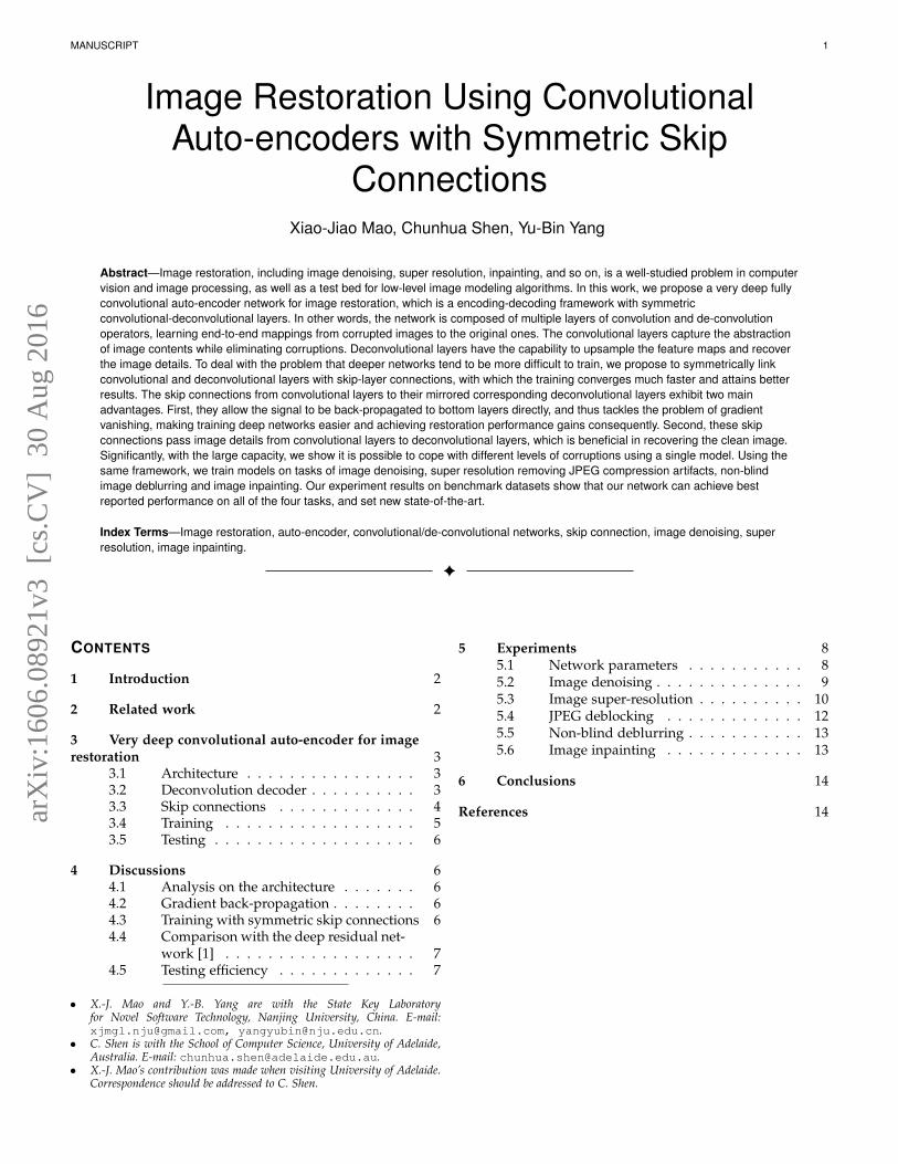
The proposed framework mainly contains a chain of con-volutional layers and symmetric deconvolutional layers, asshown in Figure 1. Skip connections are connected sym-metrically from convolutional layers to deconvolutional lay-ers. We term our method “RED-Net”—very deep ResidualEncoder-Decoder Networks.

3.1 Architecture

The framework is fully convolutional (and deconvolutional.Deconvolution is essentially unsampling convolution). Rec-tification layers are added after each convolution and de-convolution. For low-level image restoration problems, weuse neither pooling nor unpooling in the network as usuallypooling discards useful image details that are essential forthese tasks. It is worth mentioning that since the con-volutional and deconvolutional layers are symmetric, thenetwork is essentially pixel-wise prediction, thus the size ofinput image can be arbitrary. The input and output of thenetwork are images of the same size w × h × c, where w, hand c are width, height and number of channels.

Our main idea is that the convolutional layers act as afeature extractor, which preserve the primary components ofobjects in the image and meanwhile eliminating the corrup-tions. After forwarding through the convolutional layers,the corrupted input image is converted into a “clean” one.The subtle details of the image contents may be lost duringthis process. The deconvolutional layers are then combinedto recover the details of image contents. The output of thedeconvolutional layers is the recovered clean version of theinput image. Moreover, we add skip connections from aconvolutional layer to its corresponding mirrored deconvo-lutional layer. The passed convolutional feature maps aresummed to the deconvolutional feature maps element-wise,and passed to the next layer after rectification. Derivingfrom the above architecture, we have used two networksvinour experiments, which are of 20 layers and 30 layersrespectively, for image denoising, image super-resolution,JPEG deblocking and image inpainting.

3.2 Deconvolution decoder

Architectures combining layers of convolution and decon-volution [43], [44] have been proposed for semantic seg-mentation recently. In contrast to convolutional layers, inwhich multiple input activations within a filter window arefused to output a single activation, deconvolutional layersassociate a single input activation with multiple outputs.Deconvolution is usually used as learnable up-sampling layers.

In our network, the convolutional layers successivelydown-sample the input image content into a small sizeabstraction. Deconvolutional layers then up-sample the ab-straction back into its original resolution.

Besides the use of skip connections, a main differencebetween our model and [43], [44] is that our network is

MANUSCRIPT 4

Fig. 1. The overall architecture of our proposed network. The network contains layers of symmetric convolution (encoder) and deconvolution (de-coder). Skip shortcuts are connected every a few (in our experiments, two) layers from convolutional feature maps to their mirrored deconvolutionalfeature maps. The response from a convolutional layer is directly propagated to the corresponding mirrored deconvolutional layer, both forwardlyand backwardly.

fully convolutional and deconvolutional, i.e., without pool-ing and un-pooling. The reason is that for low-level imagerestoration, the aim is to eliminate low level corruptionwhile preserving image details instead of learning imageabstractions. Different from high-level applications such assegmentation or recognition, pooling typically eliminatesthe abundant image details and can deteriorate restorationperformance.

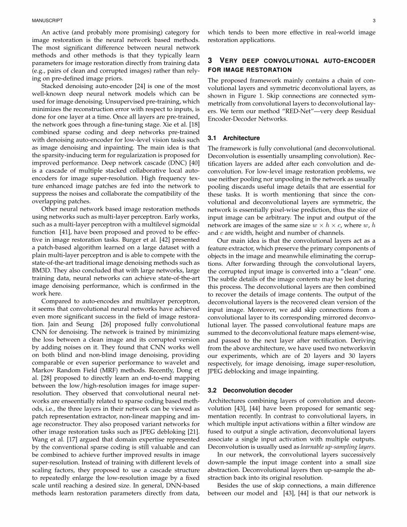
One can simply replace deconvolution with convolu-tion, which results in an architecture that is very similarto recently proposed very deep fully convolutional neuralnetworks [27], [28]. However, there exist essential differ-ences between a fully convolution model and our model.Take image denoising as an example. We compare the 5-layer and 10-layer fully convolutional network with ournetwork (combining convolution and deconvolution, butwithout skip connection). For fully convolutional networks,we use padding or up-sampling the input to make theinput and output be of the same size. For our network, thefirst 5 layers are convolutional and the second 5 layers aredeconvolutional. All the other parameters for training areidentical, i.e., trained with SGD and learning rate of 10−6,noise level σ = 70. The Peak Signal-to-Noise Ratio (PSNR)on the validation set is reported, which shows that usingdeconvolution works better than the fully convolutionalcounterpart, as shown in Figure 2.

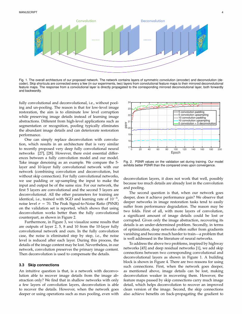
Furthermore, in Figure 3, we visualize some results thatare outputs of layer 2, 5, 8 and 10 from the 10-layer fullyconvolutional network and ours. In the fully convolutioncase, the noise is eliminated step by step, i.e., the noiselevel is reduced after each layer. During this process, thedetails of the image content may be lost. Nevertheless, in ournetwork, convolution preserves the primary image content.Then deconvolution is used to compensate the details.

3.3 Skip connections

An intuitive question is that, is a network with deconvo-lution able to recover image details from the image ab-straction only? We find that in shallow networks with onlya few layers of convolution layers, deconvolution is ableto recover the details. However, when the network goesdeeper or using operations such as max pooling, even with

Epoch0 20 40 60 80 100 120 140 160 180 200

psn

r

17

18

19

20

21

22

23

24

5 convolution padding5 convolution upsampling10 convolution padding10 convolution upsampling5 convolution + 5 deconvolution

Fig. 2. PSNR values on the validation set during training. Our modelexhibits better PSNR than the compared ones upon convergence.

deconvolution layers, it does not work that well, possiblybecause too much details are already lost in the convolutionand pooling.

The second question is that, when our network goesdeeper, does it achieve performance gain? We observe thatdeeper networks in image restoration tasks tend to easilysuffer from performance degradation. The reason may betwo folds. First of all, with more layers of convolution,a significant amount of image details could be lost orcorrupted. Given only the image abstraction, recovering itsdetails is an under-determined problem. Secondly, in termsof optimization, deep networks often suffer from gradientsvanishing and become much harder to train—a problem thatis well addressed in the literature of neural networks.

To address the above two problems, inspired by highwaynetworks [45] and deep residual networks [1], we add skipconnections between two corresponding convolutional anddeconvolutional layers as shown in Figure 1. A buildingblock is shown in Figure 4. There are two reasons for usingsuch connections. First, when the network goes deeper,as mentioned above, image details can be lost, makingdeconvolution weaker in recovering them. However, thefeature maps passed by skip connections carry much imagedetail, which helps deconvolution to recover an improvedclean version of the image. Second, the skip connectionsalso achieve benefits on back-propagating the gradient to

MANUSCRIPT 5

(a)

(b)

Fig. 3. (a) Visualization of the 10-layer fully convolutional network. Theimages from top-left to bottom-right are: clean image, noisy image, out-put of conv-2, output of conv-5, output of conv-8 and output of conv-10,where “conv-i” stands for the i-th convolutional layer; (b) Visualizationof the 10-layer convolutional and deconvolutional network. The imagesfrom top-left to bottom-right are: clean image, noisy image, output ofconv-2, output of conv-5, output of deconv-3 and output of deconv-5,where “deconv-i” stands for the i-th deconvolutional layer.

bottom layers, which makes training deeper network mucheasier as observed in [45] and [1].

Note that our skip layer connections are very differentfrom the ones proposed in [45] and [1], where the onlyconcern is on the optimization side. In our case, we wantto pass information of the convolutional feature maps tothe corresponding deconvolutional layers. The very deephighway networks [45] are essentially feedforward longshort-term memory (LSTMs) with forget gates, and theCNN layers of deep residual network [1] are feedforwardLSTMs without gates. Note that our networks are in generalnot in the format of standard feedforward LSTMs.

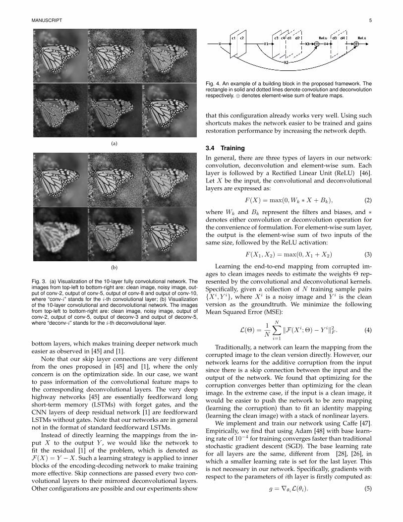
Instead of directly learning the mappings from the in-put X to the output Y , we would like the network tofit the residual [1] of the problem, which is denoted asF(X) = Y −X . Such a learning strategy is applied to innerblocks of the encoding-decoding network to make trainingmore effective. Skip connections are passed every two con-volutional layers to their mirrored deconvolutional layers.Other configurations are possible and our experiments show

Fig. 4. An example of a building block in the proposed framework. Therectangle in solid and dotted lines denote convolution and deconvolutionrespectively. ⊕ denotes element-wise sum of feature maps.

that this configuration already works very well. Using suchshortcuts makes the network easier to be trained and gainsrestoration performance by increasing the network depth.

3.4 TrainingIn general, there are three types of layers in our network:convolution, deconvolution and element-wise sum. Eachlayer is followed by a Rectified Linear Unit (ReLU) [46].Let X be the input, the convolutional and deconvolutionallayers are expressed as:

F (X) = max(0,Wk ∗X +Bk), (2)

where Wk and Bk represent the filters and biases, and ∗denotes either convolution or deconvolution operation forthe convenience of formulation. For element-wise sum layer,the output is the element-wise sum of two inputs of thesame size, followed by the ReLU activation:

F (X1, X2) = max(0, X1 +X2) (3)

Learning the end-to-end mapping from corrupted im-ages to clean images needs to estimate the weights Θ rep-resented by the convolutional and deconvolutional kernels.Specifically, given a collection of N training sample pairs{Xi, Y i}, where Xi is a noisy image and Y i is the cleanversion as the groundtruth. We minimize the followingMean Squared Error (MSE):

L(Θ) =1

N

N∑i=1

‖F(Xi; Θ)− Y i‖2F . (4)

Traditionally, a network can learn the mapping from thecorrupted image to the clean version directly. However, ournetwork learns for the additive corruption from the inputsince there is a skip connection between the input and theoutput of the network. We found that optimizing for thecorruption converges better than optimizing for the cleanimage. In the extreme case, if the input is a clean image, itwould be easier to push the network to be zero mapping(learning the corruption) than to fit an identity mapping(learning the clean image) with a stack of nonlinear layers.

We implement and train our network using Caffe [47].Empirically, we find that using Adam [48] with base learn-ing rate of 10−4 for training converges faster than traditionalstochastic gradient descent (SGD). The base learning ratefor all layers are the same, different from [28], [26], inwhich a smaller learning rate is set for the last layer. Thisis not necessary in our network. Specifically, gradients withrespect to the parameters of ith layer is firstly computed as:

g = ∇θiL(θi). (5)

MANUSCRIPT 6

Then, the two momentum vectors are computed as:

m = β1m+ (1− β1)g, v = β2v + (1− β2)g2. (6)

The update rule is:

α = α√

1− βt2/(1− βt1), θi = θi − αm/(√v + ε). (7)

β1, β2 and ε are set as the recommended values in [48].300 images from the Berkeley Segmentation Dataset

(BSD) [49] are used to generate image patches as the trainingset for each image restoration task.

3.5 TestingAlthough trained on local patches, our network can performrestoration on images of arbitrary sizes. Given a testing im-age, one can simply go forward through the network, whichis already able to outperform existing methods. To achieveeven better results, we propose to process a corrupted imageon multiple orientations. Different from segmentation, thefilter kernels in our network only eliminate the corruptions,which is usually not sensitive to the orientation of imagecontents in low level restoration tasks. Therefore, we canrotate and mirror flip the kernels and perform forwardmultiple times, and then average the output to achieve anensemble of multiple tests. We see that this can lead toslightly better performance.

4 DISCUSSIONS

4.1 Analysis on the architectureAssume that we have a network with L layers, and skipconnections are passed every layer in the first half of thenetwork. For the convenience of presentation, we denote Fcand Fd the convolution and deconvolution operation in eachlayer and do not use ReLU. According to the architecturedescribed in the last section, we can obtain the output of thei-th layer as follows:

Xi =

{XL−i + Fd(Xi−1), i ≥ L/2;Fc(Xi−1). i < L/2.

(8)

It is easy to observe that our skip connections indicateidentity mapping. The output of the network is:

XL = X0 + Fd(XL−1). (9)

Recursively, we can compute XL more specifically as fol-lows according to Equation (8):

XL = X0 + Fd(XL−1)

= X0 + Fd(X1 + Fd(XL−2))

= X0 + Fd(X1) + F 2d (X2 + Fd(XL−3))

......

= X0 + Fd(X1) + F 2d (X2) + ...+ F

L/2−1d (XL/2−1)

+ FL/2d (XL/2).

(10)Since FL/2d (XL/2) can be expressed as FL/2d (F

L/2c (X0)), we

convert Equation (10) as:

XL = FL/2d (FL/2c (X0)) +

L/2−1∑i=0

F id(Xi). (11)

In Equation (11), the term FL/2d (F

L/2c (X0)) is actually the

output of the given network without skip connections. Thedifference here is that by adopting the skip connection, wedecode each feature maps Xi, 0 ≤ i < L/2 in the firsthalf network and integrate them to the output. The mostsignificant benefit is that they carry important image details,which helps to reconstruct clean image. Moreover, the term∑L/2−1i=0 F id(Xi) indicates that these details are represented

at different levels. It is intuitive to see the following fact.It may not be easy to tell what information is needed forreconstructing clean images using only one feature mapsencoding the image abstraction; but much easier if there aremultiple feature maps encoding different levels of imageabstraction.

4.2 Gradient back-propagationFor back-propagation, a layer receives gradients from thelayers that it is connected to. As an example shown in Figure4, X is the input of the first layer, after two convolutionallayers c1 and c2, the output is X1. To update the parametersrepresented as θ2 of c2, we compute the derivative of Lwithrespect to θ2 as follows:

∇θ2L(θ2) =∂L∂X1

∂X1

∂θ2+

∂L∂X2

∂X2

∂θ2(12)

where using X1 and X2 is only for the clarity of presenta-tion, they are essentially the same. We can further formulate(12) as:

∇θ2L(θ2) =∂L∂X4

∂X4

∂X3

∂X3

∂X1

∂X1

∂θ2+

∂L∂X4

∂X4

∂X2

∂X2

∂θ2. (13)

Only ∂L∂X4

∂X4

∂X3

∂X3

∂X1

∂X1

∂θ2is computed if we do not use skip

connections, and its magnitide may become very smallafter back-propagating through many layers from the topin very deep networks. However, ∂L

∂X4

∂X4

∂X2

∂X2

∂θ2carries larger

gradients since it does not have to go through layers of d2,d1, c4 and c3 in this example. Thus with the first term only,it is more unlikely to approach zero grdients. As we can see,the skip connection helps to update the filters in bottomslayers, and thus makes training easier.

4.3 Training with symmetric skip connectionsThe aim of restoration is to eliminate corruption whilepreserving the image details as mush as possible. Previ-ous works typically use shallow networks for low-levelimage restoration tasks. The reason may be that deepernetworks can destroy the image details, which is undesiredfor pixel-wise dense regression. Even worse, using verydeep networks may easily suffer from training issues suchas gradient vanishing. Using skip connections in a very deepnetwork can address both of the above two problems.

Firstly, we design experiments to show that using skipconnections is beneficial for image detail presering. Specifi-cally, two networks are trained for image denoising with anoise level of σ = 70.

(a) In the first network, we use 5 layers of 3× 3 convolu-tion with stride 3. The input size of training data is 243×243,which results in a vector after 5 layers of convolution,encoding the very high level abstraction of the image. Thendeconvolution is used to recover the input from the feature

MANUSCRIPT 7

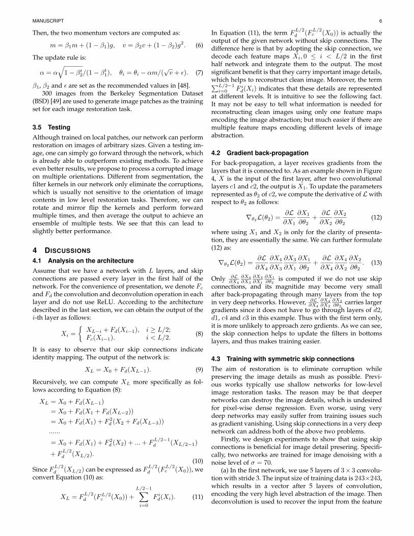
vector. The results are shown in Figure 5. We can observethat it is challenging for deconvolution to recover detailsfrom only a vector encoding the abstraction of the input.This phenomenon implies that simply using deep networksfor image restoration may not lead to satisfactory results.

(b) The second network uses the same settings as thefirst one, but adding skip connections. The results are showin Figure 5. Compared to the first network, the one with skipconnections can recover the input and achieves much betterPSNR values. This is easy to understand since the featuremaps with abundant details at bottom layers are directlypassed to the top layers.

Fig. 5. Recovering image details using deconvolution and skip connec-tions. Skip connections are beneficial in recovering image details.

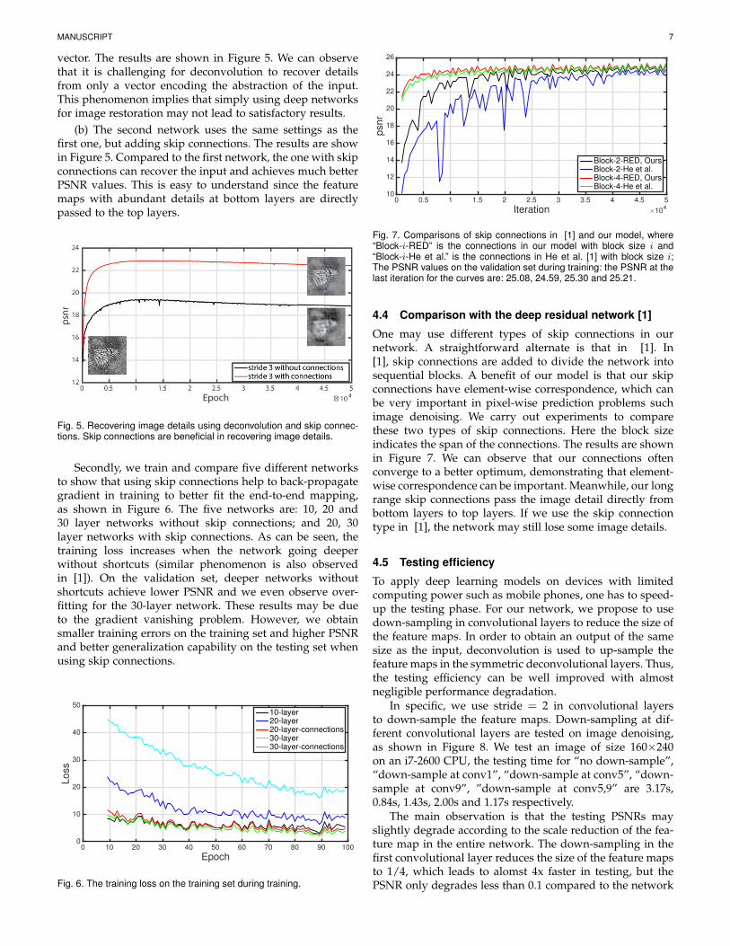
Secondly, we train and compare five different networksto show that using skip connections help to back-propagategradient in training to better fit the end-to-end mapping,as shown in Figure 6. The five networks are: 10, 20 and30 layer networks without skip connections; and 20, 30layer networks with skip connections. As can be seen, thetraining loss increases when the network going deeperwithout shortcuts (similar phenomenon is also observedin [1]). On the validation set, deeper networks withoutshortcuts achieve lower PSNR and we even observe over-fitting for the 30-layer network. These results may be dueto the gradient vanishing problem. However, we obtainsmaller training errors on the training set and higher PSNRand better generalization capability on the testing set whenusing skip connections.

Epoch0 10 20 30 40 50 60 70 80 90 100

Lo

ss

0

10

20

30

40

5010-layer20-layer20-layer-connections30-layer30-layer-connections

Fig. 6. The training loss on the training set during training.

Iteration ×104

0 0.5 1 1.5 2 2.5 3 3.5 4 4.5 5

psn

r

10

12

14

16

18

20

22

24

26

Block-2-RED, OursBlock-2-He et al.Block-4-RED, OursBlock-4-He et al.

Fig. 7. Comparisons of skip connections in [1] and our model, where“Block-i-RED” is the connections in our model with block size i and“Block-i-He et al.” is the connections in He et al. [1] with block size i;The PSNR values on the validation set during training: the PSNR at thelast iteration for the curves are: 25.08, 24.59, 25.30 and 25.21.

4.4 Comparison with the deep residual network [1]

One may use different types of skip connections in ournetwork. A straightforward alternate is that in [1]. In[1], skip connections are added to divide the network intosequential blocks. A benefit of our model is that our skipconnections have element-wise correspondence, which canbe very important in pixel-wise prediction problems suchimage denoising. We carry out experiments to comparethese two types of skip connections. Here the block sizeindicates the span of the connections. The results are shownin Figure 7. We can observe that our connections oftenconverge to a better optimum, demonstrating that element-wise correspondence can be important. Meanwhile, our longrange skip connections pass the image detail directly frombottom layers to top layers. If we use the skip connectiontype in [1], the network may still lose some image details.

4.5 Testing efficiency

To apply deep learning models on devices with limitedcomputing power such as mobile phones, one has to speed-up the testing phase. For our network, we propose to usedown-sampling in convolutional layers to reduce the size ofthe feature maps. In order to obtain an output of the samesize as the input, deconvolution is used to up-sample thefeature maps in the symmetric deconvolutional layers. Thus,the testing efficiency can be well improved with almostnegligible performance degradation.

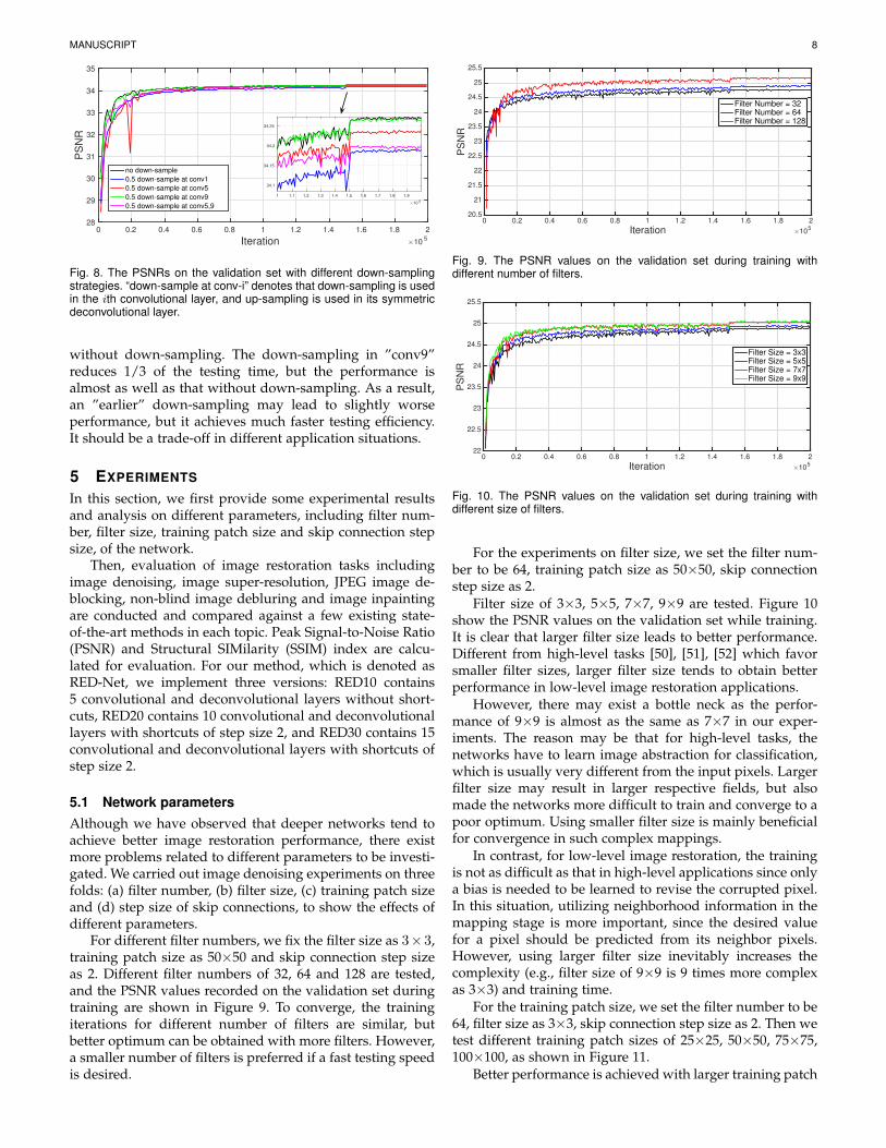
In specific, we use stride = 2 in convolutional layersto down-sample the feature maps. Down-sampling at dif-ferent convolutional layers are tested on image denoising,as shown in Figure 8. We test an image of size 160×240on an i7-2600 CPU, the testing time for “no down-sample”,“down-sample at conv1”, “down-sample at conv5”, “down-sample at conv9”, ”down-sample at conv5,9” are 3.17s,0.84s, 1.43s, 2.00s and 1.17s respectively.

The main observation is that the testing PSNRs mayslightly degrade according to the scale reduction of the fea-ture map in the entire network. The down-sampling in thefirst convolutional layer reduces the size of the feature mapsto 1/4, which leads to alomst 4x faster in testing, but thePSNR only degrades less than 0.1 compared to the network

MANUSCRIPT 8

Iteration ×105

0 0.2 0.4 0.6 0.8 1 1.2 1.4 1.6 1.8 2

PS

NR

28

29

30

31

32

33

34

35

no down-sample

0.5 down-sample at conv1

0.5 down-sample at conv5

0.5 down-sample at conv9

0.5 down-sample at conv5,9×10 5

1 1.1 1.2 1.3 1.4 1.5 1.6 1.7 1.8 1.9

34.1

34.15

34.2

34.25

Fig. 8. The PSNRs on the validation set with different down-samplingstrategies. “down-sample at conv-i” denotes that down-sampling is usedin the ith convolutional layer, and up-sampling is used in its symmetricdeconvolutional layer.

without down-sampling. The down-sampling in ”conv9”reduces 1/3 of the testing time, but the performance isalmost as well as that without down-sampling. As a result,an ”earlier” down-sampling may lead to slightly worseperformance, but it achieves much faster testing efficiency.It should be a trade-off in different application situations.

5 EXPERIMENTS

In this section, we first provide some experimental resultsand analysis on different parameters, including filter num-ber, filter size, training patch size and skip connection stepsize, of the network.

Then, evaluation of image restoration tasks includingimage denoising, image super-resolution, JPEG image de-blocking, non-blind image debluring and image inpaintingare conducted and compared against a few existing state-of-the-art methods in each topic. Peak Signal-to-Noise Ratio(PSNR) and Structural SIMilarity (SSIM) index are calcu-lated for evaluation. For our method, which is denoted asRED-Net, we implement three versions: RED10 contains5 convolutional and deconvolutional layers without short-cuts, RED20 contains 10 convolutional and deconvolutionallayers with shortcuts of step size 2, and RED30 contains 15convolutional and deconvolutional layers with shortcuts ofstep size 2.

5.1 Network parametersAlthough we have observed that deeper networks tend toachieve better image restoration performance, there existmore problems related to different parameters to be investi-gated. We carried out image denoising experiments on threefolds: (a) filter number, (b) filter size, (c) training patch sizeand (d) step size of skip connections, to show the effects ofdifferent parameters.

For different filter numbers, we fix the filter size as 3×3,training patch size as 50×50 and skip connection step sizeas 2. Different filter numbers of 32, 64 and 128 are tested,and the PSNR values recorded on the validation set duringtraining are shown in Figure 9. To converge, the trainingiterations for different number of filters are similar, butbetter optimum can be obtained with more filters. However,a smaller number of filters is preferred if a fast testing speedis desired.

Iteration ×105

0 0.2 0.4 0.6 0.8 1 1.2 1.4 1.6 1.8 2

PS

NR

20.5

21

21.5

22

22.5

23

23.5

24

24.5

25

25.5

Filter Number = 32

Filter Number = 64

Filter Number = 128

Fig. 9. The PSNR values on the validation set during training withdifferent number of filters.

Iteration ×105

0 0.2 0.4 0.6 0.8 1 1.2 1.4 1.6 1.8 2P

SN

R

22

22.5

23

23.5

24

24.5

25

25.5

Filter Size = 3x3

Filter Size = 5x5

Filter Size = 7x7

Filter Size = 9x9

Fig. 10. The PSNR values on the validation set during training withdifferent size of filters.

For the experiments on filter size, we set the filter num-ber to be 64, training patch size as 50×50, skip connectionstep size as 2.

Filter size of 3×3, 5×5, 7×7, 9×9 are tested. Figure 10show the PSNR values on the validation set while training.It is clear that larger filter size leads to better performance.Different from high-level tasks [50], [51], [52] which favorsmaller filter sizes, larger filter size tends to obtain betterperformance in low-level image restoration applications.

However, there may exist a bottle neck as the perfor-mance of 9×9 is almost as the same as 7×7 in our exper-iments. The reason may be that for high-level tasks, thenetworks have to learn image abstraction for classification,which is usually very different from the input pixels. Largerfilter size may result in larger respective fields, but alsomade the networks more difficult to train and converge to apoor optimum. Using smaller filter size is mainly beneficialfor convergence in such complex mappings.

In contrast, for low-level image restoration, the trainingis not as difficult as that in high-level applications since onlya bias is needed to be learned to revise the corrupted pixel.In this situation, utilizing neighborhood information in themapping stage is more important, since the desired valuefor a pixel should be predicted from its neighbor pixels.However, using larger filter size inevitably increases thecomplexity (e.g., filter size of 9×9 is 9 times more complexas 3×3) and training time.

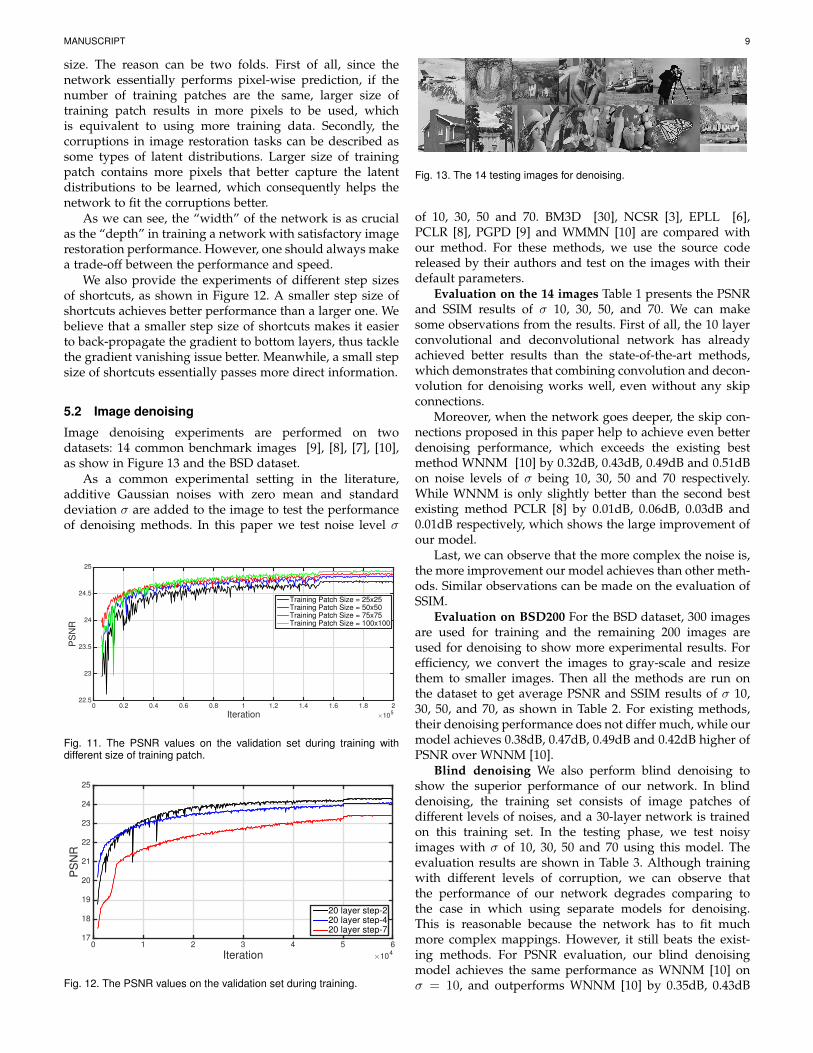
For the training patch size, we set the filter number to be64, filter size as 3×3, skip connection step size as 2. Then wetest different training patch sizes of 25×25, 50×50, 75×75,100×100, as shown in Figure 11.

Better performance is achieved with larger training patch

MANUSCRIPT 9

size. The reason can be two folds. First of all, since thenetwork essentially performs pixel-wise prediction, if thenumber of training patches are the same, larger size oftraining patch results in more pixels to be used, whichis equivalent to using more training data. Secondly, thecorruptions in image restoration tasks can be described assome types of latent distributions. Larger size of trainingpatch contains more pixels that better capture the latentdistributions to be learned, which consequently helps thenetwork to fit the corruptions better.

As we can see, the “width” of the network is as crucialas the “depth” in training a network with satisfactory imagerestoration performance. However, one should always makea trade-off between the performance and speed.

We also provide the experiments of different step sizesof shortcuts, as shown in Figure 12. A smaller step size ofshortcuts achieves better performance than a larger one. Webelieve that a smaller step size of shortcuts makes it easierto back-propagate the gradient to bottom layers, thus tacklethe gradient vanishing issue better. Meanwhile, a small stepsize of shortcuts essentially passes more direct information.

5.2 Image denoising

Image denoising experiments are performed on twodatasets: 14 common benchmark images [9], [8], [7], [10],as show in Figure 13 and the BSD dataset.

As a common experimental setting in the literature,additive Gaussian noises with zero mean and standarddeviation σ are added to the image to test the performanceof denoising methods. In this paper we test noise level σ

Iteration ×105

0 0.2 0.4 0.6 0.8 1 1.2 1.4 1.6 1.8 2

PS

NR

22.5

23

23.5

24

24.5

25

Training Patch Size = 25x25Training Patch Size = 50x50Training Patch Size = 75x75Training Patch Size = 100x100

Fig. 11. The PSNR values on the validation set during training withdifferent size of training patch.

Iteration ×104

0 1 2 3 4 5 6

PS

NR

17

18

19

20

21

22

23

24

25

20 layer step-220 layer step-420 layer step-7

Fig. 12. The PSNR values on the validation set during training.

Fig. 13. The 14 testing images for denoising.

of 10, 30, 50 and 70. BM3D [30], NCSR [3], EPLL [6],PCLR [8], PGPD [9] and WMMN [10] are compared withour method. For these methods, we use the source codereleased by their authors and test on the images with theirdefault parameters.

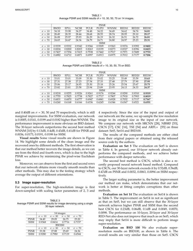
Evaluation on the 14 images Table 1 presents the PSNRand SSIM results of σ 10, 30, 50, and 70. We can makesome observations from the results. First of all, the 10 layerconvolutional and deconvolutional network has alreadyachieved better results than the state-of-the-art methods,which demonstrates that combining convolution and decon-volution for denoising works well, even without any skipconnections.

Moreover, when the network goes deeper, the skip con-nections proposed in this paper help to achieve even betterdenoising performance, which exceeds the existing bestmethod WNNM [10] by 0.32dB, 0.43dB, 0.49dB and 0.51dBon noise levels of σ being 10, 30, 50 and 70 respectively.While WNNM is only slightly better than the second bestexisting method PCLR [8] by 0.01dB, 0.06dB, 0.03dB and0.01dB respectively, which shows the large improvement ofour model.

Last, we can observe that the more complex the noise is,the more improvement our model achieves than other meth-ods. Similar observations can be made on the evaluation ofSSIM.

Evaluation on BSD200 For the BSD dataset, 300 imagesare used for training and the remaining 200 images areused for denoising to show more experimental results. Forefficiency, we convert the images to gray-scale and resizethem to smaller images. Then all the methods are run onthe dataset to get average PSNR and SSIM results of σ 10,30, 50, and 70, as shown in Table 2. For existing methods,their denoising performance does not differ much, while ourmodel achieves 0.38dB, 0.47dB, 0.49dB and 0.42dB higher ofPSNR over WNNM [10].

Blind denoising We also perform blind denoising toshow the superior performance of our network. In blinddenoising, the training set consists of image patches ofdifferent levels of noises, and a 30-layer network is trainedon this training set. In the testing phase, we test noisyimages with σ of 10, 30, 50 and 70 using this model. Theevaluation results are shown in Table 3. Although trainingwith different levels of corruption, we can observe thatthe performance of our network degrades comparing tothe case in which using separate models for denoising.This is reasonable because the network has to fit muchmore complex mappings. However, it still beats the exist-ing methods. For PSNR evaluation, our blind denoisingmodel achieves the same performance as WNNM [10] onσ = 10, and outperforms WNNM [10] by 0.35dB, 0.43dB

MANUSCRIPT 10

TABLE 1Average PSNR and SSIM results of σ 10, 30, 50, 70 on 14 images.

PSNRBM3D EPLL NCSR PCLR PGPD WNNM RED10 RED20 RED30

σ = 10 34.18 33.98 34.27 34.48 34.22 34.49 34.62 34.74 34.81σ = 30 28.49 28.35 28.44 28.68 28.55 28.74 28.95 29.10 29.17σ = 50 26.08 25.97 25.93 26.29 26.19 26.32 26.51 26.72 26.81σ = 70 24.65 24.47 24.36 24.79 24.71 24.80 24.97 25.23 25.31

SSIMσ = 10 0.9339 0.9332 0.9342 0.9366 0.9309 0.9363 0.9374 0.9392 0.9402σ = 30 0.8204 0.8200 0.8203 0.8263 0.8199 0.8273 0.8327 0.8396 0.8423σ = 50 0.7427 0.7354 0.7415 0.7538 0.7442 0.7517 0.7571 0.7689 0.7733σ = 70 0.6882 0.6712 0.6871 0.6997 0.6913 0.6975 0.7012 0.7177 0.7206

TABLE 2Average PSNR and SSIM results of σ 10, 30, 50, 70 on BSD.

PSNRBM3D EPLL NCSR PCLR PGPD WNNM RED10 RED20 RED30

σ = 10 33.01 33.01 33.09 33.30 33.02 33.25 33.49 33.59 33.63σ = 30 27.31 27.38 27.23 27.54 27.33 27.48 27.79 27.90 27.95σ = 50 25.06 25.17 24.95 25.30 25.18 25.26 25.54 25.67 25.75σ = 70 23.82 23.81 23.58 23.94 23.89 23.95 24.13 24.33 24.37

SSIMσ = 10 0.9218 0.9255 0.9226 0.9261 0.9176 0.9244 0.9290 0.9310 0.9319σ = 30 0.7755 0.7825 0.7738 0.7827 0.7717 0.7807 0.7918 0.7993 0.8019σ = 50 0.6831 0.6870 0.6777 0.6947 0.6841 0.6928 0.7032 0.7117 0.7167σ = 70 0.6240 0.6168 0.6166 0.6336 0.6245 0.6346 0.6367 0.6521 0.6551

and 0.40dB on σ = 30, 50 and 70 respectively, which is stillmarginal improvements. For SSIM evaluation, our networkis 0.0005, 0.0141, 0.0199 and 0.0182 higher than WNNM. Theperformance improvement is more obvious on BSD dataset.The 30-layer network outperforms the second best methodWNNM [10] by 0.13dB, 0.4dB, 0.43dB, 0.41dB for PSNR and0.0036, 0.0173, 0.0191, 0.0198 for SSIM.

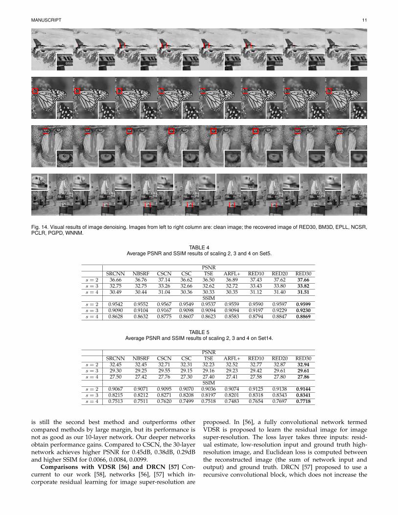
Visual results Some visual results are shown in Figure14. We highlight some details of the clean image and therecovered ones by different methods. The first observation isthat our method better recovers the image details, as we cansee from the third and fourth rows, which is due to the highPSNR we achieve by minimizing the pixel-wise Euclideanloss.

Moreover, we can observe from the first and second rowsthat our network obtains more visually smooth results thanother methods. This may due to the testing strategy whichaverage the output of different orientations.

5.3 Image super-resolutionFor super-resolution, The high-resolution image is firstdown-sampled with scaling factor parameters of 2, 3 and

TABLE 3Average PSNR and SSIM results for image denoising using a single

30-layer network.

14 imagesσ = 10 σ = 30 σ = 50 σ = 70

PSNR 34.49 29.09 26.75 25.20SSIM 0.9368 0.8414 0.7716 0.7157

BSD200σ = 10 σ = 30 σ = 50 σ = 70

PSNR 33.38 27.88 25.69 24.36SSIM 0.9280 0.7980 0.7119 0.6544

4 respectively. Since the size of the input and output ofour network are the same, we up-sample the low-resolutionimage to its original size as the input of our network.We compare our network with SRCNN [28], NBSRF [53],CSCN [17], CSC [16], TSE [54] and ARFL+ [55] on threedataset: Set5, Set14 and BSD100.

The results of the compared methods are either citedfrom their original papers or obtained using the releasedsource code by the authors.

Evaluation on Set 5 The evaluation on Set5 is shownin Table 4. In general, our 10-layer network already out-performs the compared methods, and we achieve betterperformance with deeper networks.

The second best method is CSCN, which is also a re-cently proposed neural network based method. Comparedto CSCN, our 30-layer network exceeds it by 0.52dB, 0.56dB,0.47dB on PSNR and 0.0032, 0.0063, 0.0094 on SSIM respec-tively.

The larger scaling parameter is, the better improvementour method can make, which demonstrates that our net-work is better at fitting complex corruptions than othermethods.

Evaluation on Set 14 The evaluation on Set14 is shownin Table 5. The improvement on Set14 in not as significantas that on Set5, but we can still observe that the 30-layernetwork achieves higher PSNR and SSIM than the secondbest CSCN for 0.23dB, 0.06dB, 0.1dB and 0.0049, 0.0070,0.0098. The performance on 10-layer, 20-layer and 30-layerRED-Net also does not improve that much as on Set5, whichmay imply that Set14 is more difficult to perform imagesuper-resolution.

Evaluation on BSD 100 We also evaluate super-resolution results on BSD100, as shown in Table 6. Theoverall results are very similar than those on Set5. CSCN

MANUSCRIPT 11

Fig. 14. Visual results of image denoising. Images from left to right column are: clean image; the recovered image of RED30, BM3D, EPLL, NCSR,PCLR, PGPD, WNNM.

TABLE 4Average PSNR and SSIM results of scaling 2, 3 and 4 on Set5.

PSNRSRCNN NBSRF CSCN CSC TSE ARFL+ RED10 RED20 RED30

s = 2 36.66 36.76 37.14 36.62 36.50 36.89 37.43 37.62 37.66s = 3 32.75 32.75 33.26 32.66 32.62 32.72 33.43 33.80 33.82s = 4 30.49 30.44 31.04 30.36 30.33 30.35 31.12 31.40 31.51

SSIMs = 2 0.9542 0.9552 0.9567 0.9549 0.9537 0.9559 0.9590 0.9597 0.9599s = 3 0.9090 0.9104 0.9167 0.9098 0.9094 0.9094 0.9197 0.9229 0.9230s = 4 0.8628 0.8632 0.8775 0.8607 0.8623 0.8583 0.8794 0.8847 0.8869

TABLE 5Average PSNR and SSIM results of scaling 2, 3 and 4 on Set14.

PSNRSRCNN NBSRF CSCN CSC TSE ARFL+ RED10 RED20 RED30

s = 2 32.45 32.45 32.71 32.31 32.23 32.52 32.77 32.87 32.94s = 3 29.30 29.25 29.55 29.15 29.16 29.23 29.42 29.61 29.61s = 4 27.50 27.42 27.76 27.30 27.40 27.41 27.58 27.80 27.86

SSIMs = 2 0.9067 0.9071 0.9095 0.9070 0.9036 0.9074 0.9125 0.9138 0.9144s = 3 0.8215 0.8212 0.8271 0.8208 0.8197 0.8201 0.8318 0.8343 0.8341s = 4 0.7513 0.7511 0.7620 0.7499 0.7518 0.7483 0.7654 0.7697 0.7718

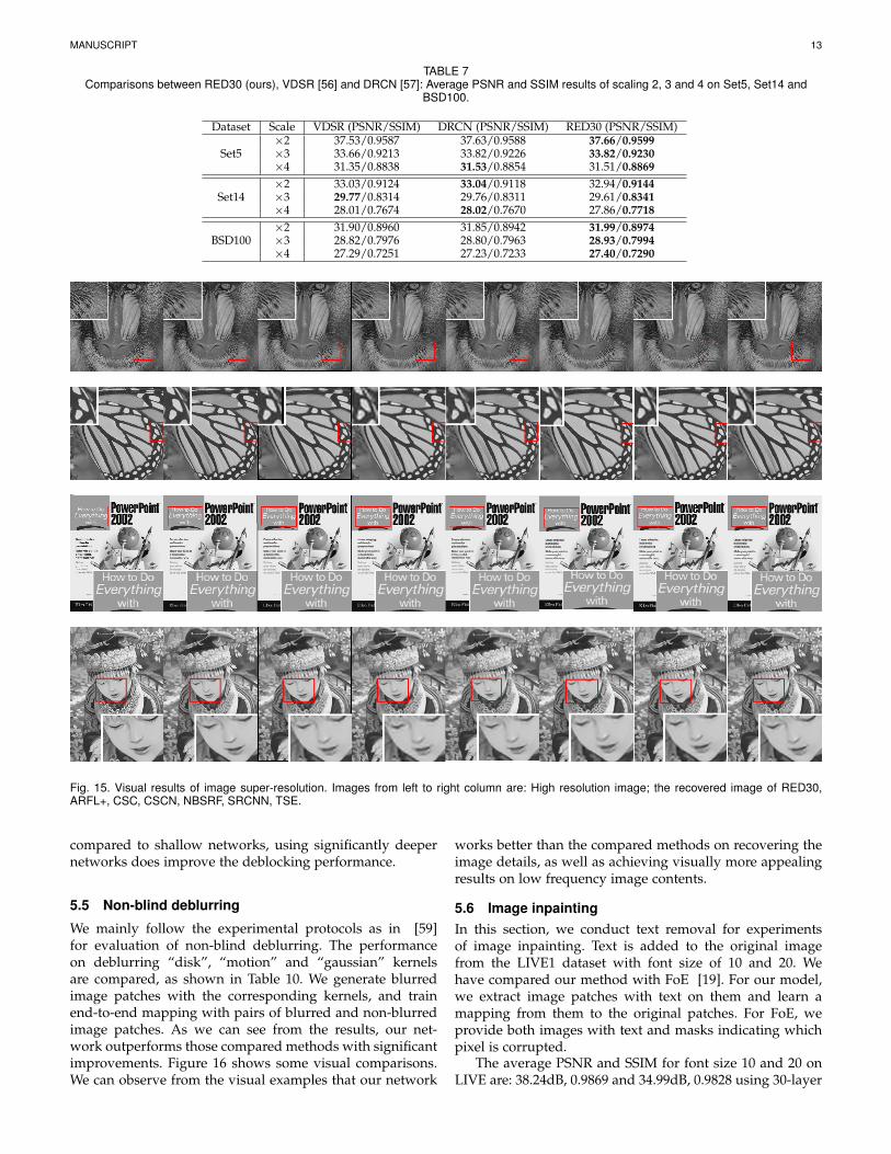
is still the second best method and outperforms othercompared methods by large margin, but its performance isnot as good as our 10-layer network. Our deeper networksobtain performance gains. Compared to CSCN, the 30-layernetwork achieves higher PSNR for 0.45dB, 0.38dB, 0.29dBand higher SSIM for 0.0066, 0.0084, 0.0099.

Comparisons with VDSR [56] and DRCN [57] Con-current to our work [58], networks [56], [57] which in-corporate residual learning for image super-resolution are

proposed. In [56], a fully convolutional network termedVDSR is proposed to learn the residual image for imagesuper-resolution. The loss layer takes three inputs: resid-ual estimate, low-resolution input and ground truth high-resolution image, and Euclidean loss is computed betweenthe reconstructed image (the sum of network input andoutput) and ground truth. DRCN [57] proposed to use arecursive convolutional block, which does not increase the

MANUSCRIPT 12

TABLE 6Average PSNR and SSIM results of scaling 2, 3 and 4 on BSD100

PSNRSRCNN NBSRF CSCN CSC TSE ARFL+ RED10 RED20 RED30

s = 2 31.36 31.30 31.54 31.27 31.18 31.35 31.85 31.95 31.99s = 3 28.41 28.36 28.58 28.31 28.30 28.36 28.79 28.90 28.93s = 4 26.90 26.88 27.11 26.83 26.85 26.86 27.25 27.35 27.40

SSIMs = 2 0.8879 0.8876 0.8908 0.8876 0.8855 0.8885 0.8953 0.8969 0.8974s = 3 0.7863 0.7856 0.7910 0.7853 0.7843 0.7851 0.7975 0.7993 0.7994s = 4 0.7103 0.7110 0.7191 0.7101 0.7108 0.7091 0.7238 0.7268 0.7290

number of parameters while increasing the depth of thenetwork. To ease the training, firstly each recursive layer issupervised to reconstruct the target high-resolution image(HR). The second proposal is to use a skip-connection frominput to the output. During training, the network has Doutputs, in which the dth output yd = x+ Rec(Hd). x is theinput low-resolution image, Rec() denotes the reconstruc-tion layer and Hd is the output of dth recursive layer. Thefinal loss includes three parts: (a) the Euclidean loss betweenthe ground truth and each yd; (b) the Euclidean loss betweenthe ground truth and the weighted sum of all yd; and (c) theL2 regularization on the network weights. Although skipconnections are used in our network, VDSR and DCRN toperform identity mapping, their differences are significant.

Firstly, both VDSR and DRCN use one path of connec-tions between the input and output, which actually models thecorruptions. In VDSR, the network itself is standard fullyconvolutional. DRCN uses recursive convolutional layersthat lead to multiple losses, which is different from VDSR.The skip connections in VDSR and DRCN model the super-resolution problem as learning the residual image, which ac-tually learns the corruption as in image restoration. In otherwords, the residual learning is only conducted in the input-output level (low-resolution and high-resolution images)in VDSR and DRCN. In contrast, our network uses multipleskip connections that divide the network into multiple blocks forresidual learning. Secondly, our skip connections pass imageabstraction of different levels from multiple convolutionallayers forwardly. No such information is used in VDSR andDRCN. In VDSR and DRCN, the skip connection only passthe input image. However, in our network, different levelsof image abstraction are obtained after the convolutionallayers, and they are passed to the deconvolutional layers forreconstruction. At last, our skip connections help to back-propagate gradients in different layers. In VDSR and DCRN,the skip connections do not involve in back-propagatinggradients since they connect the input and output, and thereare no weights to be updated for the input low-resolutionimage. The image super-resolution comparisons of VDSR,DRCN and our network on Set5, Set14 and BSD100 areprovided in Table 7.

Blind super-resolution The results of blind super-resolution are shown in Table 8. Among the compared meth-ods, CSCN can also deal with different scaling parametersby repeatedly enlarging the image by a smaller scalingfactor.

Our method is different from CSCN. Given a low-resolution image as input and the output size, we first up-sample the input image to the desired size, resulting in an

image with poor details. Then the image is fed into ournetwork. The output is an image of the same size withfine details. The training set consists of image patches ofdifferent scaling parameters and a single model is trained.Except that CSCN works slightly better on Set 14 with scal-ing factors 3 and 4, our network outperforms the existingmethods, showing that our network works much better inimage super-resolution even using only one single model todeal with complex corruptions.

TABLE 8Average PSNR and SSIM results for image super-resolution using a

single 30 layer network.

Set5s = 2 s = 3 s = 4

PSNR 37.56 33.70 31.33SSIM 0.9595 0.9222 0.8847

Set14s = 2 s = 3 s = 4

PSNR 32.81 29.50 27.72SSIM 0.9135 0.8334 0.7698

BSD100s = 2 s = 3 s = 4

PSNR 31.96 28.88 27.35SSIM 0.8972 0.7993 0.7276

Visual results Some visual results in grey-scale imagesare shown in Figure 15. Note that it is straightforward toperform super-resolution on color images.

We can observe from the second and third rows that ournetwork is better at obtaining high resolution edges andtext. Meanwhile, our results seem much more smooth thanothers. For faces such as the fourth row, out network stillobtains better visually results.

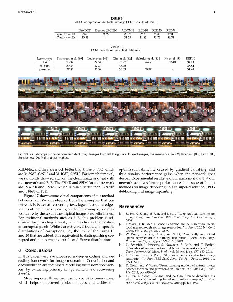
5.4 JPEG deblockingLossy compression, such as JPEG, introduces complex com-pression artifacts, particularly the blocking artifacts, ringingeffects and blurring. In this section, we carry out deblockingexperiments to recover high quality images from their JPEGcompression. As in other compression artifacts reductionmethods, standard JPEG compression schemes of JPEGquality settings q = 10 and q = 20 in MATLAB JPEGencoder are used. The LIVE1 dataset is used for evaluation,and we have compared our method with AR-CNN [21], SA-DCT [22] and deeper SRCNN [21].

The results are shown in Table 9. We can observe thatsince the Euclidean loss favors a high PSNR, our networkoutperforms other methods. Compared to AR-CNN, the 30-layer network exceeds it by 0.37dB and 0.44dB on com-pression quality of 10 and 20. Meanwhile, we can see that

MANUSCRIPT 13

TABLE 7Comparisons between RED30 (ours), VDSR [56] and DRCN [57]: Average PSNR and SSIM results of scaling 2, 3 and 4 on Set5, Set14 and

BSD100.

Dataset Scale VDSR (PSNR/SSIM) DRCN (PSNR/SSIM) RED30 (PSNR/SSIM)

Set5×2 37.53/0.9587 37.63/0.9588 37.66/0.9599×3 33.66/0.9213 33.82/0.9226 33.82/0.9230×4 31.35/0.8838 31.53/0.8854 31.51/0.8869

Set14×2 33.03/0.9124 33.04/0.9118 32.94/0.9144×3 29.77/0.8314 29.76/0.8311 29.61/0.8341×4 28.01/0.7674 28.02/0.7670 27.86/0.7718

BSD100×2 31.90/0.8960 31.85/0.8942 31.99/0.8974×3 28.82/0.7976 28.80/0.7963 28.93/0.7994×4 27.29/0.7251 27.23/0.7233 27.40/0.7290

Fig. 15. Visual results of image super-resolution. Images from left to right column are: High resolution image; the recovered image of RED30,ARFL+, CSC, CSCN, NBSRF, SRCNN, TSE.

compared to shallow networks, using significantly deepernetworks does improve the deblocking performance.

5.5 Non-blind deblurring

We mainly follow the experimental protocols as in [59]for evaluation of non-blind deblurring. The performanceon deblurring “disk”, “motion” and “gaussian” kernelsare compared, as shown in Table 10. We generate blurredimage patches with the corresponding kernels, and trainend-to-end mapping with pairs of blurred and non-blurredimage patches. As we can see from the results, our net-work outperforms those compared methods with significantimprovements. Figure 16 shows some visual comparisons.We can observe from the visual examples that our network

works better than the compared methods on recovering theimage details, as well as achieving visually more appealingresults on low frequency image contents.

5.6 Image inpaintingIn this section, we conduct text removal for experimentsof image inpainting. Text is added to the original imagefrom the LIVE1 dataset with font size of 10 and 20. Wehave compared our method with FoE [19]. For our model,we extract image patches with text on them and learn amapping from them to the original patches. For FoE, weprovide both images with text and masks indicating whichpixel is corrupted.

The average PSNR and SSIM for font size 10 and 20 onLIVE are: 38.24dB, 0.9869 and 34.99dB, 0.9828 using 30-layer

MANUSCRIPT 14

TABLE 9JPEG compression deblock: average PSNR results of LIVE1.

SA-DCT Deeper SRCNN AR-CNN RED10 RED20 RED30Quality = 10 28.65 28.92 28.98 29.24 29.33 29.35Quality = 20 30.81 - 31.29 31.63 31.71 31.73

TABLE 10PSNR results on non-blind deblurring.

kernel tpye Krishnan et al. [60] Levin et al. [61] Cho et al. [62] Schuler et al. [63] Xu et al. [59] RED30disk 25.94 24.54 23.97 24.67 26.01 32.13

motion 30.34 37.80 33.25 - - 38.84gaussian 27.90 32.34 30.09 30.97 - 34.49

Fig. 16. Visual comparisons on non-blind deblurring. Images from left to right are: blurred images, the results of Cho [62], Krishnan [60], Levin [61],Schuler [63], Xu [59] and our method.

RED-Net, and they are much better than those of FoE, whichare 34.59dB, 0.9762 and 31.10dB, 0.9510. For scratch removal,we randomly draw scratch on the clean image and test withour network and FoE. The PSNR and SSIM for our networkare 39.41dB and 0.9923, which is much better than 32.92dBand 0.9686 of FoE.

Figure 17 shows some visual comparisons of our methodbetween FoE. We can observe from the examples that ournetwork is better at recovering text, logos, faces and edgesin the natural images. Looking on the first example, one maywonder why the text in the original image is not eliminated.For traditional methods such as FoE, this problem is ad-dressed by providing a mask, which indicates the locationof corrupted pixels. While our network is trained on specificdistributions of corruptions, i.e., the text of font sizes 10and 20 that are added. It is equivalent to distinguishing cor-rupted and non-corrupted pixels of different distributions.

6 CONCLUSIONS

In this paper we have proposed a deep encoding and de-coding framework for image restoration. Convolution anddeconvolution are combined, modeling the restoration prob-lem by extracting primary image content and recoveringdetails.

More importantly,we propose to use skip connections,which helps on recovering clean images and tackles the

optimization difficulty caused by gradient vanishing, andthus obtains performance gains when the network goesdeeper. Experimental results and our analysis show that ournetwork achieves better performance than state-of-the-artmethods on image denoising, image super-resolution, JPEGdeblocking and image inpainting.

REFERENCES

[1] K. He, X. Zhang, S. Ren, and J. Sun, “Deep residual learning forimage recognition,” in Proc. IEEE Conf. Comp. Vis. Patt. Recogn.,2016.

[2] J. Mairal, F. R. Bach, J. Ponce, G. Sapiro, and A. Zisserman, “Non-local sparse models for image restoration,” in Proc. IEEE Int. Conf.Comp. Vis., 2009, pp. 2272–2279.

[3] W. Dong, L. Zhang, G. Shi, and X. Li, “Nonlocally centralizedsparse representation for image restoration,” IEEE Trans. ImageProcess., vol. 22, no. 4, pp. 1620–1630, 2013.

[4] U. Schmidt, J. Jancsary, S. Nowozin, S. Roth, and C. Rother,“Cascades of regression tree fields for image restoration,” IEEETrans. Pattern Anal. Mach. Intell., vol. 38, no. 4, pp. 677–689, 2016.

[5] U. Schmidt and S. Roth, “Shrinkage fields for effective imagerestoration,” in Proc. IEEE Conf. Comp. Vis. Patt. Recogn., 2014, pp.2774–2781.

[6] D. Zoran and Y. Weiss, “From learning models of natural imagepatches to whole image restoration,” in Proc. IEEE Int. Conf. Comp.Vis., 2011, pp. 479–486.

[7] H. Liu, R. Xiong, J. Zhang, and W. Gao, “Image denoising viaadaptive soft-thresholding based on non-local samples,” in Proc.IEEE Conf. Comp. Vis. Patt. Recogn., 2015, pp. 484–492.

MANUSCRIPT 15

Fig. 17. Visual results of our method and FoE. Images from left to right are: Corrupted images, the inpainting results of FoE and the inpaintingresults of our method. We see better recovered details as shown in the zoomed patches.

MANUSCRIPT 16

[8] F. Chen, L. Zhang, and H. Yu, “External patch prior guidedinternal clustering for image denoising,” in Proc. IEEE Int. Conf.Comp. Vis., 2015, pp. 603–611.

[9] J. Xu, L. Zhang, W. Zuo, D. Zhang, and X. Feng, “Patch groupbased nonlocal self-similarity prior learning for image denoising,”in Proc. IEEE Int. Conf. Comp. Vis., 2015, pp. 244–252.

[10] S. Gu, L. Zhang, W. Zuo, and X. Feng, “Weighted nuclear normminimization with application to image denoising,” in Proc. IEEEConf. Comp. Vis. Patt. Recogn., 2014, pp. 2862–2869.

[11] R. Timofte, V. D. Smet, and L. J. V. Gool, “A+: adjusted anchoredneighborhood regression for fast super-resolution,” in Proc. AsianConf. Comp. Vis., 2014, pp. 111–126.

[12] J. Yang, Z. Lin, and S. Cohen, “Fast image super-resolution basedon in-place example regression,” in Proc. IEEE Conf. Comp. Vis.Patt. Recogn., 2013, pp. 1059–1066.

[13] Y. Zhu, Y. Zhang, and A. L. Yuille, “Single image super-resolutionusing deformable patches,” in Proc. IEEE Conf. Comp. Vis. Patt.Recogn., 2014, pp. 2917–2924.

[14] Y. Zhu, Y. Zhang, B. Bonev, and A. L. Yuille, “Modeling deformablegradient compositions for single-image super-resolution,” in Proc.IEEE Conf. Comp. Vis. Patt. Recogn., 2015, pp. 5417–5425.

[15] G. Riegler, S. Schulter, M. Ruther, and H. Bischof, “Conditionedregression models for non-blind single image super-resolution,”in Proc. IEEE Int. Conf. Comp. Vis., 2015, pp. 522–530.

[16] S. Gu, W. Zuo, Q. Xie, D. Meng, X. Feng, and L. Zhang, “Convo-lutional sparse coding for image super-resolution,” in Proc. IEEEInt. Conf. Comp. Vis., 2015, pp. 1823–1831.

[17] Z. Wang, D. Liu, J. Yang, W. Han, and T. S. Huang, “Deep networksfor image super-resolution with sparse prior,” in Proc. IEEE Int.Conf. Comp. Vis., 2015, pp. 370–378.

[18] J. Xie, L. Xu, and E. Chen, “Image denoising and inpainting withdeep neural networks,” in Proc. Advances in Neural Inf. Process.Syst., 2012, pp. 350–358.

[19] S. Roth and M. J. Black, “Fields of experts,” Int. J. Comput. Vision,vol. 82, no. 2, pp. 205–229, 2009.

[20] J. Mairal, M. Elad, and G. Sapiro, “Sparse representation for colorimage restoration,” IEEE Trans. Image Process., vol. 17, no. 1, pp.53–69, 2008.

[21] C. Dong, Y. Deng, C. C. Loy, and X. Tang, “Compression artifactsreduction by a deep convolutional network,” in Proc. IEEE Int.Conf. Comp. Vis., 2015, pp. 576–584.

[22] A. Foi, V. Katkovnik, and K. O. Egiazarian, “Pointwise shape-adaptive DCT for high-quality denoising and deblocking ofgrayscale and color images,” IEEE Trans. Image Process., vol. 16,no. 5, pp. 1395–1411, 2007.

[23] J. Jancsary, S. Nowozin, and C. Rother, “Loss-specific training ofnon-parametric image restoration models: A new state of the art,”in Proc. Eur. Conf. Comp. Vis., 2012, pp. 112–125.

[24] P. Vincent, H. Larochelle, Y. Bengio, and P. Manzagol, “Extractingand composing robust features with denoising autoencoders,” inProc. Int. Conf. Mach. Learn., 2008, pp. 1096–1103.

[25] Y. Bengio, P. Lamblin, D. Popovici, and H. Larochelle, “Greedylayer-wise training of deep networks,” in Proc. Advances in NeuralInf. Process. Syst., 2006, pp. 153–160.

[26] V. Jain and H. S. Seung, “Natural image denoising with convo-lutional networks,” in Proc. Advances in Neural Inf. Process. Syst.,2008, pp. 769–776.

[27] J. Long, E. Shelhamer, and T. Darrell, “Fully convolutional net-works for semantic segmentation,” in Proc. IEEE Conf. Comp. Vis.Patt. Recogn., 2015, pp. 3431–3440.

[28] C. Dong, C. C. Loy, K. He, and X. Tang, “Image super-resolutionusing deep convolutional networks,” IEEE Trans. Pattern Anal.Mach. Intell., vol. 38, no. 2, pp. 295–307, 2016.

[29] P. Milanfar, “A tour of modern image filtering: New insights andmethods, both practical and theoretical,” IEEE Signal Process. Mag.,vol. 30, no. 1, pp. 106–128, 2013.

[30] K. Dabov, A. Foi, V. Katkovnik, and K. O. Egiazarian, “Imagedenoising by sparse 3-d transform-domain collaborative filtering,”IEEE Trans. Image Processing, vol. 16, no. 8, pp. 2080–2095, 2007.

[31] Z. Wang, Y. Yang, Z. Wang, S. Chang, J. Yang, and T. S. Huang,“Learning super-resolution jointly from external and internal ex-amples,” IEEE Trans. Image Process., vol. 24, no. 11, pp. 4359–4371,2015.

[32] P. Chatterjee and P. Milanfar, “Clustering-based denoising withlocally learned dictionaries,” IEEE Trans. Image Process., vol. 18,no. 7, pp. 1438–1451, 2009.

[33] L. I. Rudin, S. Osher, and E. Fatemi, “Nonlinear total variationbased noise removal algorithms,” Phys. D, vol. 60, no. 1-4, pp.259–268, November 1992.

[34] T. Chan, S. Esedoglu, F. Park, and A. Yip, “Recent developmentsin total variation image restoration,” in In Mathematical Models ofComputer Vision. Springer Verlag, 2005.

[35] J. Oliveira, J. Bioucas-Dias, and M. A. T. Figueiredo, “Adaptivetotal variation image deblurring: a majorization-minimization ap-proach,” Signal Processing, vol. 89, no. 9, pp. 2479–2493, September2009.

[36] M. Elad and M. Aharon, “Image denoising via sparse and redun-dant representations over learned dictionaries,” IEEE Trans. ImageProcess., vol. 15, no. 12, pp. 3736–3745, 2006.

[37] W. Dong, L. Zhang, G. Shi, and X. Wu, “Image deblurring andsuper-resolution by adaptive sparse domain selection and adap-tive regularization,” IEEE Trans. Image Process., vol. 20, no. 7, pp.1838–1857, 2011.

[38] K. I. Kim and Y. Kwon, “Single-image super-resolution usingsparse regression and natural image prior,” IEEE Trans. PatternAnal. Mach. Intell., vol. 32, no. 6, pp. 1127–1133, 2010.

[39] J. Yang, J. Wright, T. S. Huang, and Y. Ma, “Image super-resolutionvia sparse representation,” IEEE Trans. Image Process., vol. 19,no. 11, pp. 2861–2873, 2010.

[40] Z. Cui, H. Chang, S. Shan, B. Zhong, and X. Chen, “Deep networkcascade for image super-resolution,” in Proc. Eur. Conf. Comp. Vis.,2014, pp. 49–64.

[41] K. Sivakumar and U. B. Desai, “Image restoration using a mul-tilayer perceptron with a multilevel sigmoidal function,” IEEETrans. Signal Processing, vol. 41, no. 5, pp. 2018–2022, 1993.

[42] H. C. Burger, C. J. Schuler, and S. Harmeling, “Image denoising:Can plain neural networks compete with BM3D?” in Proc. IEEEConf. Comp. Vis. Patt. Recogn., 2012, pp. 2392–2399.

[43] H. Noh, S. Hong, and B. Han, “Learning deconvolution networkfor semantic segmentation,” in Proc. IEEE Int. Conf. Comp. Vis.,2015, pp. 1520–1528.

[44] S. Hong, H. Noh, and B. Han, “Decoupled deep neural networkfor semi-supervised semantic segmentation,” in Proc. Advances inNeural Inf. Process. Syst., 2015.

[45] R. K. Srivastava, K. Greff, and J. Schmidhuber, “Training very deepnetworks,” in Proc. Advances in Neural Inf. Process. Syst., 2015.

[46] V. Nair and G. E. Hinton, “Rectified linear units improve restrictedboltzmann machines,” in Proc. Int. Conf. Mach. Learn., 2010, pp.807–814.

[47] Y. Jia, E. Shelhamer, J. Donahue, S. Karayev, J. Long, R. Girshick,S. Guadarrama, and T. Darrell, “Caffe: Convolutional architecturefor fast feature embedding,” in Proc. ACM Int. Conf. Multimedia,2014, pp. 675–678.

[48] D. P. Kingma and J. Ba, “Adam: A method for stochastic optimiza-tion,” in Proc. Int. Conf. Learning Representations, 2015.

[49] D. Martin, C. Fowlkes, D. Tal, and J. Malik, “A database of hu-man segmented natural images and its application to evaluatingsegmentation algorithms and measuring ecological statistics,” inProc. IEEE Int. Conf. Comp. Vis., vol. 2, July 2001, pp. 416–423.

[50] M. D. Zeiler and R. Fergus, “Visualizing and understanding con-volutional networks,” in Proc. Eur. Conf. Comp. Vis., 2014.

[51] P. Sermanet, D. Eigen, X. Zhang, M. Mathieu, R. Fergus, andY. LeCun, “OverFeat: Integrated recognition, localization anddetection using convolutional networks,” Proc. Int. Conf. Learn.Representations, 2014.

[52] K. Simonyan and A. Zisserman, “Very deep convolutional net-works for large-scale image recognition,” Proc. Int. Conf. Learn.Representations, 2015.

[53] J. Salvador and E. Perez-Pellitero, “Naive bayes super-resolutionforest,” in Proc. IEEE Int. Conf. Comp. Vis., 2015, pp. 325–333.

[54] J. Huang, A. Singh, and N. Ahuja, “Single image super-resolutionfrom transformed self-exemplars,” in Proc. IEEE Conf. Comp. Vis.Patt. Recogn., 2015, pp. 5197–5206.

[55] S. Schulter, C. Leistner, and H. Bischof, “Fast and accurate imageupscaling with super-resolution forests,” in Proc. IEEE Conf. Comp.Vis. Patt. Recogn., 2015, pp. 3791–3799.

[56] J. Kim, J. K. Lee, and K. M. Lee, “Accurate image super-resolutionusing very deep convolutional networks,” in Proc. IEEE Conf.Comp. Vis. Patt. Recogn., 2016.

[57] ——, “Deeply-recursive convolutional network for image super-resolution,” in Proc. IEEE Conf. Comp. Vis. Patt. Recogn., 2016.

[58] X. Mao, C. Shen, and Y. Yang, “Image denoising using very deepfully convolutional encoder-decoder networks with symmetric

MANUSCRIPT 17

skip connections,” in Proc. Advances in Neural Inf. Process. Syst.,2016.

[59] L. Xu, J. S. J. Ren, C. Liu, and J. Jia, “Deep convolutional neuralnetwork for image deconvolution,” in Proc. Advances in Neural Inf.Process. Syst., 2014, pp. 1790–1798.

[60] D. Krishnan and R. Fergus, “Fast image deconvolution usinghyper-laplacian priors,” in Proc. Advances in Neural Inf. Process.Syst., 2009, pp. 1033–1041.

[61] A. Levin, R. Fergus, F. Durand, and W. T. Freeman, “Image anddepth from a conventional camera with a coded aperture,” ACMTrans. Graph., vol. 26, no. 3, p. 70, 2007.

[62] S. Cho, J. Wang, and S. Lee, “Handling outliers in non-blind imagedeconvolution,” in Proc. IEEE Int. Conf. Comp. Vis., 2011, pp. 495–502.

[63] C. J. Schuler, H. C. Burger, S. Harmeling, and B. Scholkopf, “Amachine learning approach for non-blind image deconvolution,”in Proc. IEEE Conf. Comp. Vis. Patt. Recogn., 2013, pp. 1067–1074.