Research in Astron. Astrophys. 20XX Vol. X No. XX, 000–000

http://www.raa-journal.org http://www.iop.org/journals/raaResearch inAstronomy andAstrophysics

Manifestations of Magnetic Bright Points observed in G-band and

Ca II H by Hinode/SOT

Yanxiao Liu1,2,3, Ning Wu4, Jun Lin1,3

1 Yunnan Observatories, Chinese Academy of Sciences, P. O. Box 110, Kunming, Yunnan 650216, P.R. China liuyanxiao@ynao.ac.cn

2 University of Chinese Academy of Sciences, Beijing 100039, P. R. China3 Center for Astro-nomical Mega-Science, Chinese Academy of Sciences, Beijing, 100012, P. R.

China4 School of Tourism and Geography, Yunnan Normal University, Kunming, Yunnan 650500, P. R.

China

Received 2018 March 20; accepted 2018 May 15

Abstract An algorithm was developed for identifying and tracking the magnetic brightpoint, or bright point (BP) for short, observed in both the photosphere (G-band) and thechromosphere (Ca II H), as well as for pairing a photospheric BP (PBP) with its conjugatechromoshperic BP (CBP). Two sets of data observed by the Hinode/SOT in the quiet Sunnear the disk center were analyzed. About 278 PBP-CBP pairs were identified and tracked.Lifetimes of both the PBPs and CBPs follow the exponential distribution with an averagelifetime of 174 s and 163 s, respectively. We found that the differences in appearance time,disappearance time, and lifetime of the two kinds of BPs all follow the Gaussian distribu-tion, which indicates that the mechanisms of PBP and CBP formation/disintegration aredifferent. But lifetimes of PBPs and CBPs are positively correlated to one another withthe coefficient of 0.8. Furthermore, we calculated the horizontal displacement betweenthe PBP and its conjugate CBP, which follows the Gaussian function with an average andthe standard deviation of (67.7 ± 38.5) km. We also calculated the amplitude of the fluxtube shape changing which might be caused by MHD waves propagating along the fluxtube, and found that it follows exponential distribution very well.

Key words: Sun: photosphere - Sun: chromosphere - methods: observational - tech-niques: image processing

1 INTRODUCTION

Photospheric bright points (PBPs) are small scale bright features located in the inter-granular lane. Theyconsist of hot photons radiating from the deep photosphere and are considered to result from the con-vective collapse of the magnetic flux tube inside the photosphere (e.g., see also Utz et al. 2014; Webb &Roberts 1978; Spruit & Zweibel 1979; Spruit 1979; Grossmann-Doerth et al. 1998; Utz et al. 2014; Liuet al. 2018b, and references therein). When the convective collapse is invoked by the downflow insidethe magnetic flux tube, the pressure balance inside and outside a flux tube breaks down. As the colddownflow of the plasma occurs, the deep photosphere layer inside the flux tube becomes optically thin,allowing the photons in the deeper photosphere of high temperature to radiate outside and the brightersubphotospheric layer to be seen. Meanwhile, the magnetic field is strengthened by the pressure outside

2 Liu et al.

the flux tube. Therefore, a PBP is thought tightly related to the magnetic field in the photosphere (Becket al. 2007; Ishikawa et al. 2007; Muller et al. 2000; Rutten et al. 2001; Berger & Title 2001; Schussleret al. 2003; Steiner et al. 2001), and is considered as a tracer of the footpoint of the flux tube at thesurface of the photosphere as well (e.g., see also Yang et al. 2016 and references therein).

Thus, PBPs are of great interest in several aspects. First, they are the reliable footpoint tracer of theflux tube that extends from the photosphere through the chromosphere into the corona. The random walkof the flux tube as a result of the convection in the photosphere (Abramenko et al. 2011; Yang et al. 2015,2016; Jafarzadeh et al. 2017, 2014a) invokes MHD waves propagating into the chromosphere and thecorona, damping the energy in these two layers of the solar atmosphere for heating (Bharti et al. 2006;Muller et al. 1994; van Ballegooijen et al. 2011; Santamaria et al. 2015; Matsumoto & Shibata 2010; Jesset al. 2012; Mumford et al. 2015; Mumford & Erdelyi 2015; Srivastava et al. 2017; Jess et al. 2009), andthe flux tube itself serves as a tunnel for the energy pumped into the upper atmosphere. Second, PBPshave relatively high intensity contrast, which could contribute to the solar irradiance variation. Third,they allow us to obtain the informations of the deeper photosphere.

With various methods of identifying and tracking, several important features of PBPs are found(see also Liu et al. 2018a for a brief review): the equivalent diameters ranging from 100 to 300 km andmanifesting a log-normal distribution (Feng et al. 2013; Ji et al. 2016; Crockett et al. 2010), lifetimesspanning over a few minutes (2-5 mins) on average (Feng et al. 2013; Wiehr et al. 2004), horizontalvelocities ranging from 1 to 3 km s−1 (Yang et al. 2014; Keys et al. 2013; Muller et al. 1994), andnumber densities varying from 0.32 (Bovelet & Wiehr 2008) and 0.97 Mm−2 (Sanchez Almeida et al.2010). These pieces of information, together with that of the magnetic field, can help us figure out thetime scale, rate, and energetics of the energy convection and temperature from the photosphere to thecorona, and further help us establish the reliable theory and model for forecasting the solar activity anderuption.

Flux tubes traced by PBPs expand their length into the chromosphere, and exhibit as bright, smallscale, and point-like radiative structures when observed in the Ca II H & K spectral lines. These smallscale structures are also known as the chromospheric bright point (CBP). In the quiet chromosphere,the CBP is one of the most distinct emission features. In addition to the CBP, structures with strongemission include network elements, namely the magnetic structure located at the supergranulation cellboundary (see the red curves in the left panel of Figure 1), the “reversed granule” (see the dark cellswith the bright edges in the top right panel of Figure 1 surrounded by the red circle), and the bright grain(see the bright features in the red box at the top right panel of Figure 1) in the internetwork that is theregion in the interior of the supergranulation cell (see the quiet regions in the left panel of Figure 1).Before performing further analysis of CBPs, we need to remove these bright features from the data.

In the internetwork, the “reversed granule” exhibits intensity reversal to the photospheric granuleand the inter-granular lane. Therefore, a “reversed granule” contains dark cells and bright arc-shapededges. The bright grain, which is also known as the Ca II H & K grain, is believed to result fromhigh frequency acoustic waves invoked in the photosphere and propagating up into the chromosphere(Carlsson & Stein 1992a,b; Remling et al. 1996; Rutten & Uitenbroek 1991; Carlsson & Stein 1997).These bright grains were found to have no relationship with the magnetic field in the chromosphere byboth observations and simulations, so was the “reversed granule”. Therefore, correlating to the magneticfield is an important and unique property of CBPs for helping distinguish themselves from the brightgrain and the “reversed granule”.

CBPs are usually observed in both the network and the internetwork. A CBP appearing in thenetwork often shows 5 − 7 min oscillation in intensity (Kariyappa et al. 2005; Tritschler & Schmidt2002; McAteer et al. 2002a), and is considered resulting from the magneto-acoustic waves of short-period in the flux tube (Hasan & van Ballegooijen 2008; Kalkofen 1999; McAteer et al. 2002b). Thetransverse and the longitudinal waves excited inside the flux tube propagate into the chromosphere anddevelop into nonlinear waves by increasing their velocity exponentially (Kalkofen 1997). On the otherhand, the CBP located in the internetwork was usually observed to exhibit 3 min oscillation in brightness(Kariyappa et al. 2005; Tritschler & Schmidt 2002) and to dissipate a large amount of energy into thechromosphere (Dame & Martic 1987; Kariyappa et al. 1994; Kariyappa 1996). Furthermore, CBPs in the

Manifestations of BPs 3

Fig. 1 Images used for specifying various bright features seen in the photosphere and thechromosphere. Left panel is the magnetogram with the studied region marked by white boxand the network is marked by the red curves. The right top panel is the Ca II H image and theright bottom panel is the G-band image in the same field of view. Some of reversed granulesand bright grains are marked by the red circle and the red box, respectively.

internetwork are reported to have an average lifetime of 7 mins, a mean size of 150 km, and horizontalvelocity ranging from 1 to 2 km s−1 (Jafarzadeh et al. 2013). Tritschler & Schmidt (2002) found that nosize difference between CBPs that appear in the network and in the internetwork.

As the indicator of the flux tube in the chromosphere, CBP is very important for helping understandthe dynamics of the chromosphere. Coupling CBPs to their photopheric counterparts, and studying theirevolutionary behaviors and properties simultaneously are essential for looking into the connection ofthe chromosphere to the photosphere magnetically, as well as the implication of such a connection tothe energetics of solar activities, and to heating the chromosphere and the corona.

4 Liu et al.

Several theories and/or models of the corona heating by MHD waves have been developed. Hasanet al. (2005) noticed that the horizontal motions of the flux tube footpoints (traced by PBPs) in thephotosphere may excite fast and slow mode magneto-acoustic waves that propagate upward along theflux tube. As a result of the stratification by the gravity, the amplitude of these waves increases withthe altitude, and turns into the compressible shock heating the plasma nearby. Because the perturbationcaused by the PBP motion occurs in the environment of β ≫ 1, the mode of the consequent wave willtransform into different ones as the wave reaches the altitude of β = 1 (Rosenthal et al. 2002; Bogdanet al. 2003). After entering the region of β < 1 or β ≪ 1, the shape of magneto-acoustic waves steepens,and eventually evolves into the shock that may result in heating (Hasan & Ulmschneider 2004). Hasanet al. (2005) also found that motions of the flux tube in the photosphere with speed less than 1 km s−1

is strong enough to invoke a wave that could turn into the shock in the chromosphere.

Cranmer & van Ballegooijen (2012), Cranmer et al. (2013) and Asgari-Targhi et al. (2013) pointedout that the motion of PBP produces the Alfven wave inside the flux tube, propagating upward. Whenmeeting the interface between the photosphere and the chromosphere, and between the chromosphereand the corona, reflection and transmission of the wave took place. The turbulence is thus created by theinteraction of the forward propagating wave and the reflected wave. The turbulence eventually dampsthe energy on the nearby media and heats the atmosphere in that region after cascading.

These models commonly assumed that the waves invoked in the photosphere transport the energyinto the upper solar atmosphere without dissipation during the propagation. In reality, on the other hand,the waves, especially the Alfven wave, may cause flux tubes to oscillate horizontally when propagatingupward through the flux tube, igniting the secondary waves in the plasma surrounding the flux tube,which results in the energy leak from the flux tube to outside, and leading to the heating of the plasmaaround the flux tube as the secondary waves dissipate outside the flux tube eventually.

In this work, we are identifying and tracking both the PBPs and the corresponding CBPs in theinternetwork by analyzing the Hinode data in order to study and compare their manifestations andproperties. We describe the observation and data processing in Section 2, display the results regardingthe times of appearance and disappearance of PBPs and CBPs, as well as their lifetimes in Section 3.We discussed these results in Section 4 and finally summarize this work in Section 5.

2 OBSERVATIONS AND DATA PROCESSING

The data studied in this work were obtained by the Solar Optical Telescope (SOT) on board the Hinodesatellite. SOT has an aperture of 50 cm with the highest spatial resolution of 0.2′′ at the wavelength of3968 A. The data cover two wave bands, the G-band in 4305 A with the band width of 8 A and the CaII H band in 3968 A with the band width of 3 A, and were obtained co-spatially and simultaneously ina quiet region near the disk center with the field of view (FOV) of 28′′ × 28′′.

These data were obtained in two time intervals. The first one was on February 11, 2007 from08:00:32 UT to 09:29:59 UT lasting 89 minutes, and the second one was on February 17, 2007 from15:00:03 UT to 15:29:30 UT lasting 30 minutes. Both data sets have the same time cadence of 11 s andthe same pixel resolution of 0.054′′ pixel−1. Before analyzing the data, we perform preprocessing forthem via the approach on the basis of the SSWIDL code to obtain the data of Level 1.

2.1 Alignment

With the data sets preprocessed, we first perform the alignment for the G-band and the Ca II H bandimages separately, and then, we further align the G-band image to the conjugate Ca II H one. For eachdata set, images in both wavelengths are aligned to their previous consecutive frames via the cross-correlation method. Since the data sets were all taken in a quiet region near the disk center and eachimage contains 512 × 512 pixels, a region with 500 × 500 pixels is selected for a given frame toalign to its previous and consecutive frame. The offset with the highest cross-correlation coefficient isobtained by calculating the barycenter of the profile of the cross correlation coefficient, and each image

Manifestations of BPs 5

is then aligned to its previous images according to this offset. The precision of the alignment could reachto the sub-pixel level.

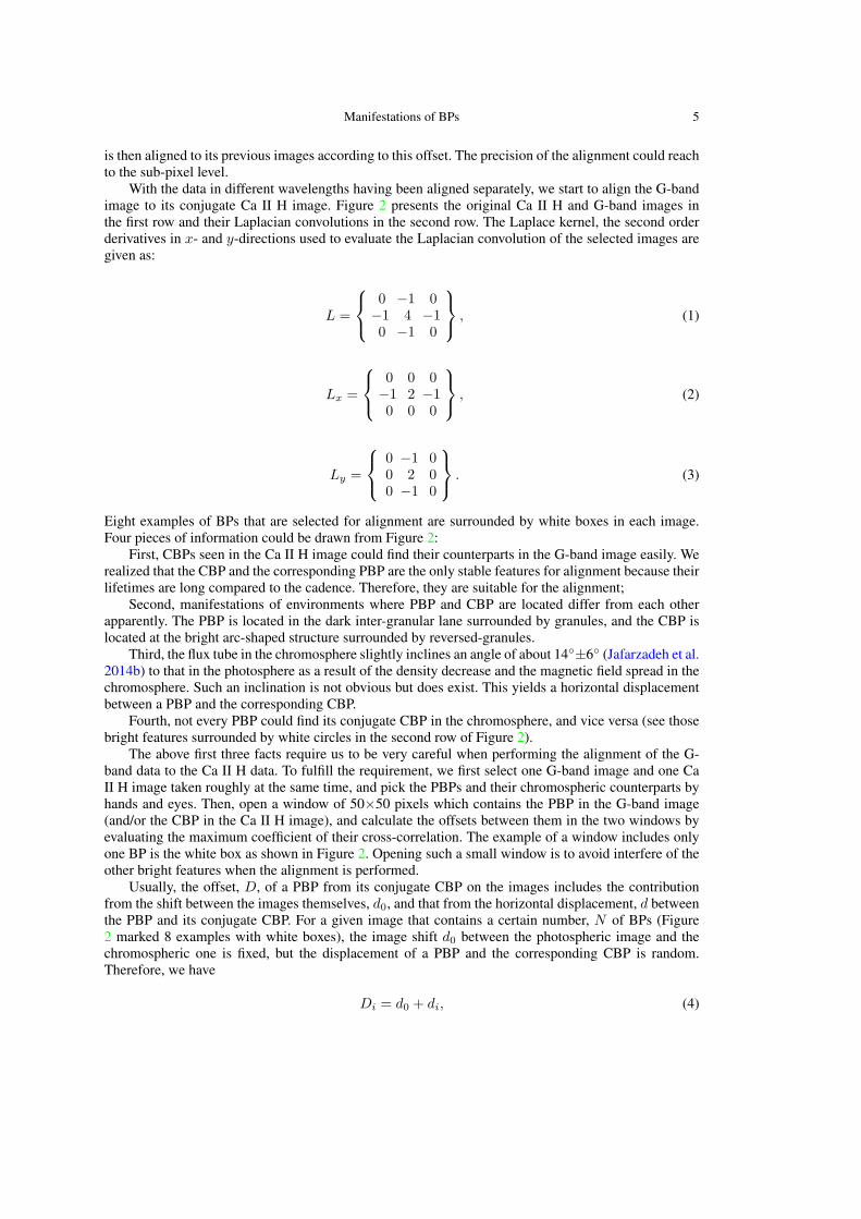
With the data in different wavelengths having been aligned separately, we start to align the G-bandimage to its conjugate Ca II H image. Figure 2 presents the original Ca II H and G-band images inthe first row and their Laplacian convolutions in the second row. The Laplace kernel, the second orderderivatives in x- and y-directions used to evaluate the Laplacian convolution of the selected images aregiven as:

L =

0 −1 0−1 4 −10 −1 0

, (1)

Lx =

0 0 0−1 2 −10 0 0

, (2)

Ly =

0 −1 00 2 00 −1 0

. (3)

Eight examples of BPs that are selected for alignment are surrounded by white boxes in each image.Four pieces of information could be drawn from Figure 2:

First, CBPs seen in the Ca II H image could find their counterparts in the G-band image easily. Werealized that the CBP and the corresponding PBP are the only stable features for alignment because theirlifetimes are long compared to the cadence. Therefore, they are suitable for the alignment;

Second, manifestations of environments where PBP and CBP are located differ from each otherapparently. The PBP is located in the dark inter-granular lane surrounded by granules, and the CBP islocated at the bright arc-shaped structure surrounded by reversed-granules.

Third, the flux tube in the chromosphere slightly inclines an angle of about 14◦±6◦ (Jafarzadeh et al.2014b) to that in the photosphere as a result of the density decrease and the magnetic field spread in thechromosphere. Such an inclination is not obvious but does exist. This yields a horizontal displacementbetween a PBP and the corresponding CBP.

Fourth, not every PBP could find its conjugate CBP in the chromosphere, and vice versa (see thosebright features surrounded by white circles in the second row of Figure 2).

The above first three facts require us to be very careful when performing the alignment of the G-band data to the Ca II H data. To fulfill the requirement, we first select one G-band image and one CaII H image taken roughly at the same time, and pick the PBPs and their chromospheric counterparts byhands and eyes. Then, open a window of 50×50 pixels which contains the PBP in the G-band image(and/or the CBP in the Ca II H image), and calculate the offsets between them in the two windows byevaluating the maximum coefficient of their cross-correlation. The example of a window includes onlyone BP is the white box as shown in Figure 2. Opening such a small window is to avoid interfere of theother bright features when the alignment is performed.

Usually, the offset, D, of a PBP from its conjugate CBP on the images includes the contributionfrom the shift between the images themselves, d0, and that from the horizontal displacement, d betweenthe PBP and its conjugate CBP. For a given image that contains a certain number, N of BPs (Figure2 marked 8 examples with white boxes), the image shift d0 between the photospheric image and thechromospheric one is fixed, but the displacement of a PBP and the corresponding CBP is random.Therefore, we have

Di = d0 + di, (4)

6 Liu et al.

Fig. 2 The original Ca II H (left) and G-band (right) images in the first row and their Laplacianconvolutions in the second row accordingly. Eight CBP-PBP pairs in the box in the first rowwere identified and paired by the eye-and-hand operation, and displayed here as examples.More BP candidates are marked by white circles in the second row.

where Di and di are the values of D and d of the ith BP, respectively. Sum this equation over all the NBPs identified in a given image, we have

N∑

i=0

Di = d0×N +

N∑

i=0

di. (5)

Manifestations of BPs 7

The random behavior of each individual value of di yields that the second term at the right hand side ofequation (5) vanishes for large enough N in principle. Then, we find

d0 = (N∑

i=0

Di)/N. (6)

In reality, we noticed that N is not necessarily very large. Usually, we take the value of d0 inequation (6) as the image shift when

|(

N+1∑

i=0

Di)/(N + 1)− (

N∑

i=0

Di)/N | (7)

is at the sub-pixel level. Then, the alignment of the G-band image to the Ca II H image could be pre-formed on the basis of d0 at the sub-pixel level. According to our experience, N could be consideredlarge enough as N = 20. After the alignment has been performed in this way for each image, the exist-ing offset for a given pair of BPs is just the horizontal displacement of the PBP from its chromosphericcounterpart only.

2.2 Identifying, Tracking, and Pairing

When preprocessing and alignment have been completed, identifying, tracking, and pairing could be pre-formed. Plenty of identifying and tracking methods have been developed previously for PBPs (Crockettet al. 2009; Xiong et al. 2016; Feng et al. 2012; Liu et al. 2018a) and for CBPs (Javaherian et al. 2014),as well as for the umbral dots (Feng et al. 2014, 2015). On the basis of these works, a new algorithm isdeveloped in this work to identify and track BPs in different atmospheric layers, and then pair the twotypes of BPs with one another.

We note here that identifying and tracking CBPs is not a trivial job since they are located in acomplex environment mixed with various structures of magnetic field and plasma. The key characteristicused for distinguishing a CBP from its complicated environment is the magnetic field because a CBP isthe intersection (or footpoint) of a magnetic flux with (at) the chromosphere, and the other bright featuresaround it like bright grains and arc-shaped structures are not related to magnetic field. According to thisproperty of CBPs, two approaches are usually used to identify CBPs. The first one is to pinpoint thebright point in the chromosphere that can be directly related to the magnetic field, which is applied byJafarzadeh et al. (2013); and the second one is to pair the CBP with its conjugate PBP and further confirmthat they are located on the same flux tube. In the present work, we are using the second approach.

Usually, We perform the same identifying and tracking operations on both the G-band and the Ca IIH data. We shall make specific explanation only when different operations are used for the G-band dataand the Ca II H data. The method used in this work consists of the following steps.

Step one, extract candidates of BPs for all the data. First of all, three kinds of convolutions betweenthe original images and the Laplace kernel, second order derivatives in x- and y-directions (CL, CLx

,CLy

) given in equations (1), (2), and (3) are calculated, respectively.

The Laplace kernel in equation (1) is an isotropic second-order differential operator that highlightsthe places with large brightness gradients and deemphasizes the places of small brightness gradients. Italso highlights the structures that are brighter than the average brightness of surroundings. Equation (2)gives the second order derivatives in x-direction and it only highlights the large brightness gradient in x-direction, and equation (3) highlights the places with large brightness gradients in y-direction. Equation(2) is more sensitive to the brightness varying in the x-direction and equation (3) is more sensitive in they-direction (refer to Gonzalez & Woods 2008, pp. 160−162 for more details).

Then, a set of thresholds are applied to extract the candidate of BPs. For each frame, the pixels withall the three convolutions, Ci (i = L,Lx, Ly), higher than 0.01 × max(Ci) are selected as the candidateof BPs.

8 Liu et al.

The candidate of PBPs extracted from the G-band data includes most of PBPs and some of brightgranules (see discussions of Liu et al. 2018b), and the candidate of CBPs extracted from the Ca II H dataincludes most of CBP and some of the bright arc-shaped structures. Because the bright granule observedin the photosphere is co-spatially related to the faint “reversed granule” in the chromosphere, and thebright arc-shaped structure in the chromosphere is related to the dark granular lane in the photosphere,among the candidates of PBPs and the conjugate CBPs, only those of the real PBP and CBP can be pairedwith one another via their positive correlation in brightness. This implies that if a bright candidate ofPBP is co-spatially related to a bright candidate of CBP, then, both candidates of CBP and PBP are theones that we are looking for; otherwise, neither of them is what we need.

Step two, remove noise. After having completed the operation at step one, we obtained PBP andCBP candidates. However, we could not perform further operations on them yet because they includenoises. Similar to what we noted previously (e.g., see Liu et al. 2018b), the noise consists of very brightgranule and its chromospheric counterpart. They were selected as candidates because the values of theirconvolutions with the Laplacian kernel exceed the threshold we set. They should be removed via theoperation similar to that used by Liu et al. (2018b) such that the candidate of size less than 5 pixelsor appearing in less than 3 consecutive images is considered as the noise and is abandoned. After thenoise has been removed, what left is the real PBP-CBP candidate. We still need to note here that thesecandidate pairs obtained here only contain the PBPs and their corresponding CBPs that are both brightat the same time, and the faint-bright and bright-faint PBP-CBP pairs are not included yet. So, we needto perform the operations to further pick the faint-bright or the bright-faint pairs up.

Step three, track BPs. The operation at this step includes two tasks: the first is to detect the BPsthat failed to be extracted at previous steps, and another one is to check whether the BPs appearing intwo consecutive images identify with each other. In order to detect all the BPs in various intensities,we set three thresholds according to the convolutions of the original image with the Laplacians givenin equations (1), (2), and (3). They are 10%, 5%, and 3% of the maximum of the convolutions, Ci

(i = L,Lx, Ly), of a given image, which are classified into the top level, the middle level, and the lowlevel, respectively. The pixels with all the three convolutions higher than the top (middle, low) levelthreshold are marked as the top (middle, low) level seeds. The pixels with any of the three convolutionslower than the low level threshold are discarded. Now, we are ready for tracking BPs, and three worksneed to be done:

(a). Each candidate is labeled with a number i (i = 1, 2, 3...N ). For candidate i in a given image, wecheck whether a candidate i′ occurs in top level seeds at the same position in previous or next consecutiveimage. If candidate i′ exists and it also overlaps at least partly with i, we consider the candidate i and i′

the same BP and label the candidate i′ with the same number of i. Furthermore, if candidate i′ has sizelarger than 8 pixels, then it is considered as a very bright BP, or it is not a bright one and we need tolower the threshold to extend its size.

(b). If no overlap occurs between the candidates i and i′, then two possibilities need to be considered.One is that candidate i′ does not exist in the same position in previous or following consecutive frame;another one is that candidate i′ does exist, but it is too faint to be detected under the threshold set inwork (a). For the second situation, we look for candidate i′ among the middle level seeds by repeatingthe operations performed in work (a).

(c). If no candidate i′ detected in either (a) or (b), then we look for a very faint candidate i′′ in thelow level seeds following the same approach taken in (a). If candidate i′ (or i′′) is detected in this wayand overlaps with candidate i, as well as possesses the size exceeding 8 pixels, then candidate i and i′ (ori′′) are considered of the same BP at different times. Otherwise, we conclude that no BP appears at thesame position in either previous or following consecutive frame. All the BP candidates can be trackedin this way, and eventually, we could detect and track every BP from its appearance to disappearance.

Step four, deduce the real size of the BP. At previous steps, we found the candidates whose sizesare just a fraction of the true BP size. Therefore, we need to find the true size of the BP. For eachcandidate, a window of a suitable size containing the region where the candidate is located, togetherwith the nearby pixels, is opened. Then, we set the boundary on pixels, at which the first derivatives ineither x- or y-direction reach maximum and the second derivatives cross zero. The edge of a BP then

Manifestations of BPs 9

consists of these pixels, and the true size of the BP could be obtained consequently (see Liu et al. 2018bfor more details).

Step five, pair the PBP with the conjugate CBP that are located on (trace) the same magnetic fluxtube extending from the photosphere to the chromosphere. If a PBP and a CBP are located on the sameflux tube, they should manifest similar evolutionary features. Such a behavior indicated that they areconjugate. This method is suitable for the BP that appear in either active or quiet region, and either onthe disk center or near the limb. In addition, a simple and straightforward approach, especially suitablefor the BP in the quiet region near the disk center, may be applied. A magnetic flux tube in this regionextends outward almost radially and along the line of sight, and the CBP and its conjugate should appearat the same location on the detector (a CCD or photograph film) plane as a result of the projection effects.Therefore, if a PBP and a CBP seen in the images taken at the same time are co-located in space duringthe interval of their lifetimes, they are considered as the pair of BPs. With these five step operationsbeing completed, we are now ready for further investigation on various behaviors of PBP-CBP pairs wehave identified.

3 RESULT

We have completed extracting and tracking BPs, as well as pairing PBPs and CBPs in previous sections.The identifying results can be checked by comparing it (see Figure 3) with the original one (Figure2). Comparing each panel in two figures, the identified features are marked with white color in Figure3 which are apparently clearer and sharper. The BPs in the circles and boxes are identified very well.However, we do not use all of these identified BPs. Only a few of them are selected in this work.

We note here that only the isolated BP is studied for simplicity in this work. Identifying and trackingboth the non-isolated PBPs and CBPs is not trivial, and pairing the non-isolated PBPs with CBPs isalmost impossible, if not completely impossible, for the time being. We shall work on this issue in thefuture. Here, an isolated BP is the one that does not experience any process of merging or splittingduring its lifetime, and a non-isolated one experiences at least merging or splitting once (e.g., see alsoLiu et al. 2018b for more discussions). Furthermore, the selected BP pairs are insured to appear in aregion that are far from the places of magnetic clusters and BP gathering in order to avoid the influenceof the environment in surroundings. We totally pinpointed 278 PBP-CBP pairs in this work.

We now start working on the information about the appearance and the disappearance of BPs,which further gives the lifetimes of BPs. This will also allow us to look into the difference in the abovemanifestation between a PBP and its conjugate CBP.

The way to determine when a BP appears or disappears is simple. For a BP we select from a frame,if no bright feature is found at the same location in the previous adjacent frame, then we take time ofthis frame as the appearance time of the BP. Similarly, if no bright feature can be detected at the samelocation in the following adjacent frame, then we take the time of this frame as the disappearance timeof the BP. Therefore, the lifetime of a BP can be deduced consequently.

For these 278 pairs of BPs, we calculated the difference in their appearing (disappearing) times,in their lifetimes, and correlations among their lifetimes. Lifetimes of both PBPs and CBPs follow theexponential distribution (Figure 4a), from which we find that the PBP lifetime is 174 s on average, withthe maximum of 726 s and the minimum of 67 s , and that the CBP lifetime is 163 s on average with themaximum of 906 s and the minimum of 67 s, respectively. We find that the lifetimes of PBPs and CBPscorrelate to one another fairly well with the correlation coefficient of 0.8 (Figure 4c).

Figure 4a further indicates that the lifetime of PBPs does not differ very much from that of CBPs,and the difference in their lifetimes follows the Gaussian distribution with the mean value of 2 s andthe full-width at the half maximum (FWHM) of 90 s. In addition, the difference in the appearing (dis-appearing) times between PBPs and the conjugate CBPs can be deduced as well, which also follow theGaussian distribution with the mean value of 13 (9) s, and FWHM of 61 (62) s (see also Figure 4b), re-spectively. Note: continuous curves are of the Gaussian function, and are used to fit the results deducedfrom observations.

10 Liu et al.

Fig. 3 Same as Figure 2 but with identified BPs highlighted and selected BPs surrounded bysquares and circles in Laplacian convolution images.

Besides various times and their differences we just discussed, another important information aboutthe dynamic property of the flux tube, as well as its essential implication for understanding the physics ofthe chromosphere and corona heating, could be deduced from values of di that have been smoothed forthe purpose of alignment in previous section. di is calculated as the horizontal displacement from gravitycenter of a CBP to that of its conjugate PBP, which result from flux tube inclinations. As mentionedearlier, an inclination of the flux tube exists as it extends from the photosphere to the chromosphere,which could cause the horizontal displacement between the cross sections in the photosphere and thechromosphere.

After operations associated with equations (4) through (7), the contribution of d0 to Di can besubtracted according to equation (4), and Di thus eventually includes contributions from inclination

Manifestations of BPs 11

0 100 200 300 400 500 600 700 800 900 1000

0.00

0.05

0.10

0.15

0.20

0.25

0.30

0.35

0.40

0.45

-400 -300 -200 -100 0 100 200 300 400 500

0.0

0.1

0.2

0.3

0.4

0.5

0.6

0.7

0.8

0.9

0 100 200 300 400 500 600 700 800

0

200

400

600

800

1000

ProbablyDensityFunction

ProbablyDensityFunction

(a) Lifetime of BPs

PBPs

CBPs

(b) Time difference [s]

In appearance time

In disappearance time

In lifetime

LifetimeofCBPs[s]

(c) Lifetime of PBPs [s]

Fig. 4 (a) lifetimes of PBPs and CBPs. Both of them are fitted to exponential functions well.(b) distributions of differences in appearing time, in disappearing time, and in lifetimes be-tween PBPs and CBPs. Three of them are fitted to Gaussian functions.(c) scatter plot betweenCBP lifetimes and PBP lifetimes with the correlation coefficient of 0.8.

0 50 100 150 200 250

0.00

0.02

0.04

0.06

0.08

0.10

0.12

-20 0 20 40 60 80 100 120 140 160 180

0.00

0.05

0.10

0.15

0.20

0.25(a)

PDF

Horizontal displacements between CBPs and PBPs [km]

(b)

Horizontal oscillation displacements of flux tubes [km]

Fig. 5 Shifts of the flux tube. The left panel is the horizontal displacement between the PBPand the CBP, and the right panel is the horizontal displacement of the flux tube caused byperturbation. The data in the left panel are fitted to a Gaussian function and those in the rightpanel are fitted to an exponential function well.

shift and wavy distortion of the flux tube only. Figure 5a displays the probability density function (PDF)of Di, which shows clearly the Gaussian pattern, from which we obtain the average and the associatedstandard deviation of Di as (67.7± 38.5) km.

In addition, the perturbation in surroundings or MHD waves traveling upward along the flux tubemight distort the flux tube, and give rise to the horizontal displacement between PBPs and CBPs, as wellas the change of the displacement. Assuming the inclination of flux tubes is fixed in the quiet region fora short time (for example, 11 s), then the difference of the displacements Di between two consecutiveframes is the amplitude of the traversing oscillation of the flux tube. The right panel in Figure 5b displaysthe distribution of this amplitude, which is fitted to an exponential function very well.

12 Liu et al.

4 DISCUSSIONS

The connection of a PBP to its conjugate CBP through a magnetic flux tube suggests the importance ofinvestigating behaviors of the two BPs in helping us understand physical courses of the energy conver-sion and transportation occuring in the photosphere and in the chromosphere, and pairing a PBP withits conjugate CBP may further reveal information on the response of the chromosphere to any change inthe photosphere.

As a follow-up of the work by Liu et al. (2018b), we developed a new method of identifying andtracking, and further pairing PBPs and CBPs. Because of the difficulty in coupling the non-isolated BPsin different layers of the solar atmosphere one to another, the focus of this work is on the isolated BPsonly.

In addition to identifying and tracking, we note here that pairing PBPs and CBPs is a new, simpleand important skill that was developed in this work. Usually, PBPs are easy to distinguish from brightgranules via size, brightness, sharp edges, and locations. However, CBPs are usually located in a com-plicated environment such that they stay in bright arc-shaped structures, and are surrounded by brightgrains in the chromosphere. This is because the magnetic field in the chromosphere gets apparentlymore complex than in the photosphere as a result of the decrease in the gas pressure. In the presentwork, we used the approach of pairing a CBP with its conjugate PBP to identify the CBP in its complexenvironment.

We studied the appearing (disappearing) times, and lifetimes of the PBP and the CBP, as well asthe difference in these times. PBP lifetimes follow the exponential distribution.The lifetime of PBPsis (174 s ± 105) s on average with minimum of 67 s and maximum of 726 s, which is in agreementwith that obtained by Xiong et al. (2017) with average lifetime of 173 s. Utz et al. (2010) reported thePBP lifetime of 2.5 mins on average, and Sanchez Almeida et al. (2004) found that most of PBPs havelifetime shorter than 10 mins in the quiet region. Keys et al. (2014) reported that PBPs in a quiet area ofthe active region have a lifetime of (88± 23) s on average. Liu et al. (2018b) obtained that the lifetimeof the isolated PBPs is (267 ± 140) s on average in active region. Abramenko et al. (2010) reported that98.6% of PBPs live less than 120 s in the quiet Sun. In this work, we find that only about 37% PBPshave lifetimes less than 120 s.

The lifetime of CBPs deduced here follows the exponential distribution as well with the averagelifetime of (163 ± 106) s, with the shortest of 67 s and the longest of 906 s, respectively. Xiong et al.(2017) found that the CBP has lifetime of 131 s on average, which is in consistent with our result. deWijn et al. (2005, 2006) reported lifetime of 258 s, and Jafarzadeh et al. (2013) of 673 s. In our results,about 42% CBPs are found to have lifetimes less than 120 s.

Several reasons exist for the different results in lifetimes. The first one is that different methodsof identifying and tracking BPs were used, and the second one is that different observation data fromdifferent telescopes with different cadences and spatial resolutions were analyzed. At last, the mostimportant one exists in the method of identifying and tracking BPs such that how to determine the BPsappearing in two consecutive frames are the same one.

In this work, we determine whether they are the same one according to their relative locations inthe two consecutive images: if the positions of the BP in the two images partly or totally overlap eachother, then they are the same one; otherwise, they are not the same one. This method helps us avoidmistracking, but it may miss some long lived and fast moving BPs as well.

From Figure 4b, we notice that the distribution of the difference in appearing times, disappearingtimes, and lifetimes of PBPs and CBPs all follow the Gaussian function with the mean value of −12.8s, 8.8 s, and 2 s, and with FWHM of 61 s, 62 s, and 90 s, respectively. Since the time cadence ofobservations is 11 s, the appearing time, disappearing time and lifetime of PBPs and their conjugateCBPs are considered the same, namely, PBPs and CBPs appear and disappear simultaneously, and thushave the same lifetime on average.

The Gaussian distribution of the differences in appearance/disappearance times indicates that theformation/disintegration of the PBP and the CBP are independent of each other. But their lifetimesare correlated to one another with the correlation coefficient of 0.8. These two results seem inconsis-

Manifestations of BPs 13

tent with each other. We understand them in this way though: Because a PBP connects to its chromo-spheric counterpart via a magnetic flux tube from the photosphere to the chromosphere, their forma-tion/disintegration are governed by the formation/disintegration of the flux tube. On the other hand, theappearance/disappearance times of PBP(CBP) are controlled by different mechanisms.

The appearance of PBPs is considered to result from the formation of the flux tube due to the con-vective collapse in the photosphere, allowing hot and bright plasma in the deeper photospheric layersto be seen; and the formation of CBPs might suggest the local heating inside the flux tube in the chro-mosphere by waves propagating from the photosphere along flux tube. Considering the fact that boththe PBP and CBP are tracers of the flux tube in the photosphere and the chromosphere, respectively, weunderstand that their lifetimes should be tightly related to that of the flux tube, and the longer the fluxtube lives, the longer the lifetime of PBP (CBP) is.

We note here that the above discussions and the consequent conclusions are on the basis of thefollowing assumptions. Because the BPs that we selected to study here were located in a very quietregion, the inclination of a flux tube is considered fixed for a short time and the absolute value of thedifference of the same PBP-CBP pair between Di and Di+1 in the two consecutive frames displays theamplitude of perturbation to the flux tube in the horizontal direction caused by the perturbation outsideor MHD waves inside the flux tube. The distribution of the amplitude shown in Figure 5b indicatesthat the probability decreases with the amplitude. Kalkofen (1997) suggested that the transverse wavesinside the flux tube propagate into the chromosphere and develop into nonlinear waves by increasingtheir velocity, and the amplitude increases with height due to the density stratification because of thegravity ( see also Hasan et al. 2005). Combining these results with the one revealed by Figure 5b, we areable to have a physical scenario: When the wave propagates upward along the flux tube with the velocityincreasing and the amplitude amplifying, the probability decreases in detecting the oscillation of the fluxtube at a fixed location with a given time cadence. This is the reason why the larger the amplitude is, thelower the probability of the amplitude being detected is as shown in Figure 5b.

5 CONCULSION

In addition to identifying and tracking PBPs and CBPs, we also paired the PBP with its conjugate CBPfor the first time. The importance of pairing the PBP with the CBP is that it does not only provide asimple method for distinguishing CBPs from their complex environment, but also helps understand howthe CBP behaves along with the PBP via flux tubes, as well as the associated physical process of theenergy conversion and transportation from the photosphere to the chromosphere.

We paired 278 PBP-CBP successfully, and found that the CBP does not always follow the motionof the PBP synchronously. Instead shifts and displacements of their locations exist apparently. Thisindicates that the change in the shape of the flux tube might be caused by MHD waves propagating alongthe flux tube, and it provides an important constraint for theories and models of the corona heating bythe wave as well.

Acknowledgements This work was supported by the Program 973 grant 2013CBA01503, NSFC grantsU1631130, 11333007 and 11763004, and CAS grants, XDA17010505, XDA15010900, and QYZDJ-SSW-SLH012. This work was also supported by the grant associated with the Project of the Group forInnovation of Yunnan Province.

References

Abramenko, V. I., Carbone, V., Yurchyshyn, V., et al. 2011, ApJ, 743, 133Abramenko, V., Yurchyshyn, V., Goode, P., & Kilcik, A. 2010, ApJ, 725, L101Asgari-Targhi, M., van Ballegooijen, A. A., Cranmer, S. R., & DeLuca, E. E. 2013, ApJ, 773, 111Beck, C., Bellot Rubio, L. R., Schlichenmaier, R., & Sutterlin, P. 2007, A&A, 472, 607Berger, T. E., & Title, A. M. 2001, ApJ, 553, 449

14 Liu et al.

Bharti, L., Jain, R., Joshi, C., & Jaaffrey, S. N. A. 2006, in Astronomical Society of the PacificConference Series, Vol. 354, Solar MHD Theory and Observations: A High Spatial ResolutionPerspective, ed. J. Leibacher, R. F. Stein, & H. Uitenbroek, 13

Bogdan, T. J., Carlsson, M., Hansteen, V. H., et al. 2003, ApJ, 599, 626Bovelet, B., & Wiehr, E. 2008, A&A, 488, 1101Carlsson, M., & Stein, R. 1992a, in Astronomical Society of the Pacific Conference Series, Vol. 26,

Cool Stars, Stellar Systems, and the Sun, ed. M. S. Giampapa & J. A. Bookbinder, 515Carlsson, M., & Stein, R. F. 1992b, ApJ, 397, L59Carlsson, M., & Stein, R. F. 1997, ApJ, 481, 500Cranmer, S. R., & van Ballegooijen, A. A. 2012, ApJ, 754, 92Cranmer, S. R., van Ballegooijen, A. A., & Woolsey, L. N. 2013, ApJ, 767, 125Crockett, P. J., Jess, D. B., Mathioudakis, M., & Keenan, F. P. 2009, MNRAS, 397, 1852Crockett, P. J., Mathioudakis, M., Jess, D. B., et al. 2010, ApJ, 722, L188Dame, L., & Martic, M. 1987, ApJ, 314, L15de Wijn, A. G., Rutten, R. J., Haverkamp, E. M. W. P., & Sutterlin, P. 2005, A&A, 441, 1183de Wijn, A. G., Rutten, R. J., Haverkamp, E. M. W. P., & Sutterlin, P. 2006, in Astronomical Society

of the Pacific Conference Series, Vol. 354, Solar MHD Theory and Observations: A High SpatialResolution Perspective, ed. J. Leibacher, R. F. Stein, & H. Uitenbroek, 20

Feng, S., Deng, L., Yang, Y., & Ji, K. 2013, Ap&SS, 348, 17Feng, S., Ji, K.-f., Deng, H., Wang, F., & Fu, X.-d. 2012, Journal of Korean Astronomical Society, 45,

167Feng, S., Xu, Z., Wang, F., et al. 2014, Sol. Phys., 289, 3985Feng, S., Zhao, Y., Yang, Y., et al. 2015, Sol. Phys., 290, 1119Grossmann-Doerth, U., Schuessler, M., & Steiner, O. 1998, A&A, 337, 928Hasan, S. S., & Ulmschneider, P. 2004, A&A, 422, 1085Hasan, S. S., & van Ballegooijen, A. A. 2008, ApJ, 680, 1542Hasan, S. S., van Ballegooijen, A. A., Kalkofen, W., & Steiner, O. 2005, ApJ, 631, 1270Ishikawa, R., Tsuneta, S., Kitakoshi, Y., et al. 2007, A&A, 472, 911Jafarzadeh, S., Cameron, R. H., Solanki, S. K., et al. 2014a, A&A, 563, A101Jafarzadeh, S., Solanki, S. K., Feller, A., et al. 2013, A&A, 549, A116Jafarzadeh, S., Solanki, S. K., Lagg, A., et al. 2014b, A&A, 569, A105Jafarzadeh, S., Solanki, S. K., Cameron, R. H., et al. 2017, ApJS, 229, 8Javaherian, M., Safari, H., Amiri, A., & Ziaei, S. 2014, Sol. Phys., 289, 3969Jess, D. B., Mathioudakis, M., Erdelyi, R., et al. 2009, Science, 323, 1582Jess, D. B., Shelyag, S., Mathioudakis, M., et al. 2012, ApJ, 746, 183Ji, K.-F., Xiong, J.-P., Xiang, Y.-Y., et al. 2016, Research in Astronomy and Astrophysics, 16, 78Kalkofen, W. 1997, ApJ, 486, L145Kalkofen, W. 1999, in Astronomical Society of the Pacific Conference Series, Vol. 184, Third Advances

in Solar Physics Euroconference: Magnetic Fields and Oscillations, ed. B. Schmieder, A. Hofmann,& J. Staude, 227

Kariyappa, R. 1996, Sol. Phys., 165, 211Kariyappa, R., Narayanan, A. S., & Dame, L. 2005, Bulletin of the Astronomical Society of India, 33,

19Kariyappa, R., Sivaraman, K. R., & Anadaram, M. N. 1994, Sol. Phys., 151, 243Keys, P. H., Mathioudakis, M., Jess, D. B., Mackay, D. H., & Keenan, F. P. 2014, A&A, 566, A99Keys, P. H., Mathioudakis, M., Jess, D. B., et al. 2013, MNRAS, 428, 3220Liu, Y., Xiang, Y., & Erdelyi, R. 2018a, ApJLiu, Y., Xiang, Y., Erdelyi, R., et al. 2018b, ApJ, 856, 17Matsumoto, T., & Shibata, K. 2010, ApJ, 710, 1857McAteer, R. T. J., Gallagher, P. T., Williams, D. R., et al. 2002a, in ESA Special Publication, Vol. 505,

SOLMAG 2002. Proceedings of the Magnetic Coupling of the Solar Atmosphere Euroconference,ed. H. Sawaya-Lacoste, 305

Manifestations of BPs 15

McAteer, R. T. J., Gallagher, P. T., Williams, D. R., et al. 2002b, ApJ, 567, L165Muller, R., Dollfus, A., Montagne, M., Moity, J., & Vigneau, J. 2000, A&A, 359, 373Muller, R., Roudier, T., Vigneau, J., & Auffret, H. 1994, A&A, 283, 232Mumford, S. J., & Erdelyi, R. 2015, MNRAS, 449, 1679Mumford, S. J., Fedun, V., & Erdelyi, R. 2015, ApJ, 799, 6Remling, B., Deubner, F.-L., & Steffens, S. 1996, A&A, 316, 196Rosenthal, C. S., Bogdan, T. J., Carlsson, M., et al. 2002, ApJ, 564, 508Rutten, R. J., Kiselman, D., Rouppe van der Voort, L., & Plez, B. 2001, in Astronomical Society of

the Pacific Conference Series, Vol. 236, Advanced Solar Polarimetry – Theory, Observation, andInstrumentation, ed. M. Sigwarth, 445

Rutten, R. J., & Uitenbroek, H. 1991, Sol. Phys., 134, 15Sanchez Almeida, J., Bonet, J. A., Viticchie, B., & Del Moro, D. 2010, ApJ, 715, L26Sanchez Almeida, J., Marquez, I., Bonet, J. A., Domınguez Cerdena, I., & Muller, R. 2004, ApJ, 609,

L91Santamaria, I. C., Khomenko, E., & Collados, M. 2015, A&A, 577, A70Schussler, M., Shelyag, S., Berdyugina, S., Vogler, A., & Solanki, S. K. 2003, ApJ, 597, L173Spruit, H. C. 1979, Sol. Phys., 61, 363Spruit, H. C., & Zweibel, E. G. 1979, Sol. Phys., 62, 15Srivastava, A. K., Shetye, J., Murawski, K., et al. 2017, Scientific Reports, 7, 43147Steiner, O., Hauschildt, P. H., & Bruls, J. 2001, A&A, 372, L13Tritschler, A., & Schmidt, W. 2002, in ESA Special Publication, Vol. 506, Solar Variability: From Core

to Outer Frontiers, ed. A. Wilson, 785Utz, D., del Toro Iniesta, J. C., Bellot Rubio, L. R., et al. 2014, ApJ, 796, 79Utz, D., Hanslmeier, A., Muller, R., et al. 2010, A&A, 511, A39van Ballegooijen, A. A., Asgari-Targhi, M., Cranmer, S. R., & DeLuca, E. E. 2011, ApJ, 736, 3Webb, A. R., & Roberts, B. 1978, Sol. Phys., 59, 249Wiehr, E., Bovelet, B., & Hirzberger, J. 2004, A&A, 422, L63Xiong, J. P., Zhang, A. L., Ji, K. F., et al. 2016, Acta Astronomica Sinica, 57, 29Xiong, J., Yang, Y., Jin, C., et al. 2017, The Astrophysical Journal, 851, 42Yang, Y.-F., Lin, J.-B., Feng, S., et al. 2014, Research in Astronomy and Astrophysics, 14, 741Yang, Y., Ji, K., Feng, S., et al. 2015, ApJ, 810, 88Yang, Y., Li, Q., Ji, K., et al. 2016, Sol. Phys., 291, 1089