Managing Flexibility: Optimal Sizing and Schedulingof Flexible Servers

Jinsheng Chen, Jing DongColumbia University, New York, NY 10027

Problem definition: We study the optimal joint staffing and scheduling problem in multi-class service systems,

where there is an option to staff flexible servers who can handle multiple classes of customers. The specific

feature we consider is that the flexible server may incur a higher cost or a loss of efficiency. We study

how flexibility is best utilized in two scenarios: one with deterministic arrival rates and the other with

random arrival rates. Academic/practical relevance: When managing resource flexibility in service systems,

the conventional wisdom is that server flexibility is beneficial due to the resource pooling effect. However,

in practice, flexibility often incurs some additional costs. Our work studies the interplay between the cost

and benefit of flexibility in managing these systems. Methodology: We utilize a heavy-traffic asymptotic

framework to develop structural insights. When there is no uncertainty in the arrival rates, we use a coupling

argument and a diffusion approximation. When the arrival rates are random, we use a stochastic-fluid

relaxation. Results: We derive asymptotically optimal joint staffing and scheduling rules for a two-class

multi-server queue with both dedicated and flexible servers. Managerial implications: Our results show that

the size of the flexible server pool is of a smaller order than the size of the dedicated pools, and the flexible

servers are mostly used to hedge against system stochasticity or demand uncertainty, depending on which

source of randomness dominates. The proposed staffing and scheduling policies are easy to implement and

achieve near-optimal performance.

1. Introduction

Service systems typically involve multiple customer classes and server types. For example, in call

centers, customers may require different types of service, and servers may be equipped with different

skill sets (Gans et al. 2003). In hospitals, patients may be classified into differential specialties, each

requiring a very different type of care, and nurses may be trained according to the care type (Best

et al. 2015). Servers can sometimes be trained to handle multiple classes (types) of customers. We

refer to these servers as flexible servers. Increasing the size of the flexible server pool can help

balance the workload between different classes of customers, and improve system performance.

Specifically, when managing queues with multiple classes of jobs, the benefit of load-balancing

and capacity flexibility have been studied and demonstrated in various settings (see, for example,

Andradottir et al. (2003), Tsitsiklis and Xu (2012)).

However, flexibility may come at a cost. First, flexible servers who are capable of performing

multiple types of tasks are typically more expensive to hire (Bassamboo et al. 2012). Second,

multi-tasking may lead to a loss of efficiency. It is well-documented in the Psychology literature

1

2

that multi-tasking incurs cognitive switching costs which hinder productivity (Pashler 1994). A

recent empirical study reveals that placing patients in the non-primary care ward can lead to worse

patient outcomes including a longer length-of-stay (Song et al. 2019). Given the cost and benefit

of flexible capacity, it is important to understand how to strike a balance in resource management.

When designing the service system, the service provider has to make multiple decisions. Chief

among them are how many of each type of server to staff and how to match customers with servers.

These problems are often referred to as the staffing and scheduling problems in the literature. In

this paper, we study the joint staffing and scheduling problem in multi-class queues with both

dedicated and flexible servers. In particular, to highlight the key tradeoff, we consider a stylized

M-model with two classes of customers and three potential pools of servers: two dedicated pools

and one flexible pool that can serve both classes of customers. To capture the cost of flexibility,

we assume that the flexible servers may be more costly to staff and may serve at a slower rate

than dedicated servers. The objective is to find the optimal staffing and scheduling policies that

minimize the sum of the staffing cost, holding cost, and abandonment cost.

We consider two demand scenarios. One has deterministic arrival rates, which is the case when

we have a very accurate estimate of customer demand. In this case, the flexible pool can be used to

hedge against stochasticity, i.e., the stochastic fluctuation of interarrival times and service times.

In particular, due to the stochasticity in system dynamics, one queue may incur a higher than

average load while the other is at or below its normal load from time to time. In such situations,

the flexible pool can be used to help the class with a heavier load, and thus balance the load

between the two classes. The other scenario has random arrival rates, which is the case when there

is a high degree of uncertainty in customer demand. In this case, the flexible pool is mainly used

to hedge against parameter uncertainty. In particular, when the realized arrival rate of one class

is higher than average while the realized arrival rate of the other class is at or below average, the

flexible pool can be used to help the class with a higher realized arrival rate, and thus balance

the load. The differences between the two scenarios described above give rise to different hedging

mechanisms, which in turn lead to different sizes of the flexible pool in optimality. To see this, let

λ denote the average arrival rate. When λ is large, the stochastic fluctuation of the system with a

given arrival rate is in general of order√λ (Garnett et al. 2002). The parameter uncertainty, on

the other hand, can be of a different order than√λ (Bassamboo et al. 2010b). Indeed, the case we

are interested in is one where the standard deviation of the random arrival rate is of a larger order

than√λ. Lastly, the different hedging mechanisms also lead to different scheduling policies in our

developments.

Because staffing and scheduling decisions interact, the joint optimization problem can be very

challenging. When arrival rates are deterministic and symmetric, we use a coupling construction

3

to derive the optimal scheduling policy for any staffing level. The scheduling policy prioritizes the

dedicated servers (faster servers) when routing customers to servers, and prioritizes the class with

more customers in the system when scheduling flexible servers, assuming the abandonment rate

is less than the service rates. Given the optimal scheduling policy, we then optimize the staffing

policy. To derive structural insights into the size of the flexible pool, we employ a heavy-traffic

asymptotic approach, where we send the arrival rate to infinity and study how the size of the

flexible pool scales with the arrival rate. Our result provides necessary and sufficient conditions

for staffing rules to be asymptotically optimal. The key insight is that when flexibility comes at a

cost, the optimal size of the flexible pool only leads to partial resource pooling. In particular, the

flexible pool helps create some load-balancing, but the effect is not large enough to equalize the

two queues asymptotically.

When arrival rates are random and the magnitude of the parameter uncertainty dominates the

system stochasticity, we employ a stochastic-fluid relaxation of the optimal staffing problem. In

this relaxation, we ignore the stochasticity of the queueing dynamics and focus on the parameter

uncertainty only. The stochastic-fluid optimization problem is a special case of the single-period

multi-product inventory problem with demand substitution, for which we can characterize the

optimal solution explicitly. The relaxation also motivates a simple scheduling rule that essentially

decomposes the M-model into two independent inverted-V models for any realization of the arrival

rates. When the average arrival rates grow to infinity, we show that the staffing and scheduling

rules derived based on the stochastic-fluid relaxation are asymptotically optimal. The key insight is

that when facing both parameter uncertainty and cost of flexibility, the optimal size of the flexible

pool provides some hedging against the parameter uncertainty, and the cost saving, compared to

the no-flexible resource case, is increasing with the magnitude of the uncertainty.

In addition to providing prescriptive solutions to managing flexibility, we also highlight the

following contributions of our work.

1. When the arrival rates are symmetric and deterministic, we construct the optimal schedul-

ing policy for any arrival rates and staffing levels. In contrast to most of the optimal scheduling

literature for multi-server queues, our results do not rely on any asymptotic argument (for devel-

opment on asymptotically optimal scheduling policies, see, for example, Atar (2005)). Instead, the

proof uses a coupling argument that can be of interest to the analysis of other Markovian queue-

ing systems. Our coupling technique also allows us to establish the optimality of a non-standard

scheduling policy when the abandonment rate is larger than the service rates, see Theorem 5.

2. When the arrival rates are deterministic and the flexible pool is of the optimal order, we derive

the diffusion limit of the M-model under heavy-traffic. The limit is a two-dimensional diffusion

process. In particular, the complete resource pooling condition is not satisfied when the flexible

4

pool is optimally sized, i.e., the flexible pool size is not large enough to instantaneously balance

the queue lengths between the two classes. Thus, we do not have state space collapse in the limit,

i.e., the two-dimensional queue length process does not reduce to a one-dimensional process in

the limit. This is in contrast to most of the optimal scheduling literature (see, for example, Dai

and Tezcan (2011), Gurvich and Whitt (2009a)). On the other hand, the limiting process cannot

be fully decomposed along each dimension, i.e., the drift terms of the two component diffusion

processes are interconnected. Thus, we achieve partial resource pooling.

3. When the arrival rates are random and the parameter uncertainty is of a larger order than the

stochasticity of the queueing dynamics, we quantify the optimality gap for policies derived based

on the stochastic fluid approximation. This extends the results in Bassamboo et al. (2010b) from

a multi-server queue with a single class of customers and a single pool of servers to a multi-class

queue with multiple server types. We also allow the arrival rate distributions of the two classes to

be asymmetric, i.e., they can have different means and different levels of uncertainty.

1.1. Literature review

We first review related works on queues with deterministic arrival rates. The M-model studied in

this paper is a special case of parallel server systems (PSSs). Due to the interplay between staffing

and scheduling decisions, the joint staffing and scheduling problem can be highly nontrivial for

general PSSs. In the literature, most works only look at one of the two problems in isolation.

However, there are a few exceptions. Noticeably, Armony and Mandelbaum (2011) consider the

joint optimization problem for an inverted-V model where there is a single class of customers and

multiple types of servers. Using a coupling argument, they establish the optimality of the fastest-

server-first policy. Gurvich and Whitt (2009b) study the problem of staffing and scheduling PSSs

to minimize total staffing costs subject to quality-of-service constraints. They establish that the

queue-and-idleness-ratio control is asymptotically optimal in heavy-traffic. When dealing with a

single class of customers and a single pool of servers, Borst et al. (2004) study the optimal staffing

problem in an M/M/n queue. They find that the quality-and-efficiency-driven (QED) regime,

which is also known as the Halfin-Whitt regime (Halfin and Whitt 1981), arises naturally when

staffing is set to balance the staffing cost and the system performance. The work is then extended

by Mandelbaum and Zeltyn (2009) to allow for customer abandonment.

The work that is most related to ours is Bassamboo et al. (2012), which studies the sizing of

flexible resources when service rates can be continuously chosen. They find that the linear staffing

and holding costs often lead to an O(√λ) flexibility when flexible capacity is more expensive. The

main difference between our work and theirs is the modeling of the service resources. They use a

single-server mode of analysis and assume the service rate can be optimally chosen. This modeling

5

approach is reasonable for computer or manufacturing systems. Motivated mostly by large-scale

service systems, our work adopts a many-server mode of analysis. As Bassamboo et al. (2012) point

out, the many-server regime that we consider introduces substantial complexity to the analysis,

and they leave this extension as a potential future research direction. In addition, Bassamboo et al.

(2012) assumes a longest-queue-first scheduling and hypothesize that it is likely to be optimal. We

establish the optimality of a scheduling policy that prioritizes the class with more customers in the

system.

More broadly, optimal scheduling of various PSSs has been extensively studied in the literature.

For example, Tezcan and Dai (2010) study the optimal scheduling of the N-model. They show that

a cµ-type of greedy policy is asymptotically optimal in the many-server QED regime. Atar (2005)

studies the optimal scheduling problem of general PSSs, i.e., with multiple classes of customers

and multiple pool of servers, and customer abandonment. The work establishes the asymptotical

optimality of policies derived based on the corresponding optimal diffusion control problem in

the many-server QED regime. Kim et al. (2018) study the optimal scheduling of V-model with

general patience-time distributions. The main feature that distinguishes our work from the stream

of works on PSSs in the QED regime is the size of our flexible server pool. In our analysis, the

size of the flexible pool is asymptotically negligible in the fluid scale, whereas in the literature, it

is almost universally assumed that the fluid-scaled pool sizes are non-negligible (see, for example,

Assumption 1 in Atar (2005), Assumption 2.1 in Gurvich and Whitt (2009a), and equation (20)

in Dai and Tezcan (2011)). Due to the difference in the size of our server pools, the asymptotic

behavior (diffusion limit) of our system can be qualitatively different from what is observed in the

literature.

When the arrival rates are random, our work is related to works that look at staffing queues

when facing parameter uncertainty. The stochastic-fluid relaxation was first proposed in Harrison

and Zeevi (2005). Its efficacy has been studied in several subsequent works. Bassamboo et al. (2006)

show that it leads to an asymptotically optimal staffing policy under a non-conventional asymptotic

regime that features large arrival rates and short service times. The asymptotic framework is then

extended in Bassamboo and Zeevi (2009), who consider the case when the arrival rate distribution

is unknown and has to be estimated from data. Compared to these works, the analysis in this paper

takes a different asymptotic approach. In particular, we increase the system demand, i.e., arrival

rates, but do not scale other system parameters such as service rates and abandonment rates. The

paper Bassamboo et al. (2010b) takes a similar heavy-traffic asymptotic approach as ours and

establishes the optimality gap of the staffing policy derived from the stochastic-fluid relaxation for

an Erlang-A model with a random arrival rate. We extend their results to a multi-class network

setting, where in addition to the staffing decision, we also have to decide on the scheduling policy.

6

Whitt (2006) develops a different stochastic-fluid model that allows non-exponential service times

and patience times, and studies the staffing problem with both random arrival rates and staffing

levels (due to employee absenteeism). When facing demand uncertainty, Gurvich et al. (2010)

study the staffing problem with a chance constraint for the quality of service. They first use mixed

integer programming to obtain a first-order staffing solution, and then refine the staffing level

using simulation. Kocaga et al. (2015) study the staffing and outsourcing problem when demand

is random.

Our work contributes to this stream of literature in two key ways. First, we show that when

dealing with random demand, it is the staffing, not the scheduling decision, that is of paramount

importance. This supports why many papers tend to focus on the staffing instead of the scheduling

decision in this setting (see, for example Gurvich et al. (2010), Bertsimas and Doan (2010)). Second,

we quantify the benefit of flexibility. Specifically, we extend the notion that the order of flexibility

should match the order of system stochasticity in Bassamboo et al. (2012) to the case where the

order of flexibility should match the order of demand uncertainty. In general, the notion that just

a small degree of flexibility is enough has been much investigated over the years in various different

contexts (see, for example, Simchi-Levi and Wei (2012), Shi et al. (2019) for manufacturing systems,

Tsitsiklis and Xu (2012), Wallace and Whitt (2005) for PSSs, etc.) Our work contributes to this

literature as well.

1.2. Paper structure and notations

In Section 2, we introduce the queueing model and the optimization problem. In Section 3, we

study the optimal scheduling and staffing policy for a symmetric M-model with deterministic

arrival rates. The goal is to highlight the cost and benefit of flexibility in a classical setting with

no parameter uncertainty. In Section 4, we study the staffing and scheduling problem for systems

with random arrival rates. To highlight the effect of demand uncertainty, we focus on the regime

where the demand uncertainty dominates the system stochasticity. We complement our theoretical

analysis with numerical experiments in Section 5. In particular, the numerical analysis focuses

on the pre-limit performance of our proposed staffing and scheduling rules. The proofs of all the

theoretical results are delayed until the Appendix.

We next introduce some notations that are used throughout the paper. The set of non-negative

integers is denoted by N0, and the set of real numbers is denoted by R. We define η(t) = 0, χ(t) = t,

and I(t) = 1, for t ≥ 0. Let D denote the space of functions from [0,∞) to R that are right-

continuous with left limits and is endowed with Skorohod J1 topology. Let ei be a unit vector with

the i-th element equal to 1. The dimension of ei depends on the context. We write 1· for the

indicator function. A random variable A is said to be stochastically larger than a random variable

7

B, A ≥st B, if P(A > x) ≥ P(B > x) for any x ∈ R. For real sequences an and bn, we say

that an =O(bn) if limsupn→∞ |an|/bn <∞, an = o(bn) if limsupn→∞ |an|/bn = 0, and an = Θ(bn) if

lim infn→∞ |an|/bn > 0. For a∈R, write a+ = max(a,0) and a− = max(−a,0).

2. The Model

We consider a classical M-model with possible demand uncertainty as depicted in Figure 1. In

particular, the model has two customer classes, Class 1 and Class 2, and three pools of servers:

two dedicated pools for the two customer classes and one flexible pool that can serve both classes.

We allow the arrival rate for Class i, Λi, i= 1,2, to be a random variable. For a given realization

of Λi, i.e., Λi = λi, Class i arrivals follow a Poisson process with rate λi. Each server pool can have

multiple servers. We write ni for the number of servers in the dedicated pool for Class i, and nF for

the number of servers in the flexible pool. If a customer is served by the dedicated server, its service

time follows an exponential distribution with rate µ. If a customer is served by the flexible server,

its service time follows an exponential distribution with rate µF . We assume µF ≤ µ to account

for the potential efficiency loss of flexible servers. Each customer has a patience time that follows

an exponential distribution with rate θ. Once a customer’s waiting time (in the queue) exceeds its

patience time, it abandons the system.

… … …µ µ µ µ µ µµF µF

nFn1 n2

Λ1 Λ2

θ θ

Figure 1 The M-model

For i= 1,2, let Xi(t) denote the number of Class i customers in the system at time t. We denote

Zi(t) and ZFi(t) as the number of dedicated servers and flexible servers serving Class i customers

at time t respectively. Note that

Zi(t)≤ ni,ZF (t) :=ZF1(t) +ZF2(t)≤ nF , and Zi(t) +ZFi(t)≤Xi(t). (1)

Let Qi(t) denote the number of Class i customers waiting in the queue at time t. Then Qi(t) =

Xi(t)−Zi(t)−ZFi(t). Let X(t) := (X1(t),X2(t)), Z(t) := (Z1(t),Z2(t),ZF1(t),ZF2(t)), and Q(t) :=

8

(Q1(t),Q2(t)). We also define the total number of customers in the system and the total queue

length processes as XΣ(t) =X1(t)+X2(t) and QΣ(t) =Q1(t)+Q2(t) respectively. Let Ai, Si, SFi,Gi

be independent unit-rate Poisson processes, which will be used to represent the arrival, departure,

and abandonment events respectively. At the beginning of the planning horizon Λi is realized.

Given Λi = λi, Xi(t) satisfies the following dynamics:

Xi(t) =Xi(0) +Ai (λit)−Gi

(θ

∫ t

0

Qi(s)ds

)−Si

(µ

∫ t

0

Zi(s)ds

)−SFi

(µF

∫ t

0

ZFi(s)ds

).

To fully describe dynamics of the system, we need to specify the scheduling policy – how to

allocate the servers. We restrict ourselves to preemptive deterministic Markovian policies, where

the allocation of servers Z(t) can be viewed as a function of the current state of the system X(t)

(Harrison and Zeevi 2004). Let ν denote such a policy (mapping), i.e., Z(t) = ν(Xλ(t)) and it

satisfies the feasibility conditions listed in (1).

Let QΣ(∞;n1, n2, nF ;ν) be the steady-state total queue length given staffing level (n1, n2, nF )

and scheduling policy ν. If the system is not stable under a certain staffing and scheduling rule,

we define QΣ(∞;n1, n2, nF ;ν)≡∞. Our goal is to jointly choose the staffing levels for each pool

and the scheduling policy to minimize the sum of the staffing costs and the steady-state average

holding and abandonment costs:

minn1,n2,nF ,ν

Π(n1, n2, nF ;ν) := c(n1 +n2) + cFnF + (h+ aθ)E[QΣ(∞;n1, n2, nF ;ν)], (2)

where c > 0 is the per server per unit time staffing cost for the dedicated pools, cF > 0 is the per

server per unit time staffing cost for the flexible pool, h > 0 is the per customer per unit time

holding cost, and a> 0 is the per customer abandonment cost. Note that the abandonment cost is

aθE[QΣ(∞;n1, n2, nF ;ν)] because θE[QΣ(∞;n1, n2, nF ;ν)] is the rate at which customers abandon

in stationarity. We also note that

E[QΣ(∞;n1, n2, nF ;ν)] =E[E[QΣ(∞;n1, n2, nF ;ν)|Λ]],

where E[QΣ(∞;n1, n2, nF ;ν)|Λ = (λ1, λ2)] is the steady-state average queue length of an M-model

with arrival rates (λ1, λ2), and the outer expectation is taken with respect to the random arrival

rates Λ, i.e., the demand uncertainty.

In order to avoid trivial situations, we impose the following condition on the rates and cost

parameters:

c/µ< cF/µF <h/θ+ a. (3)

The first inequality ensures that flexible servers have some disadvantage over dedicated servers.

Otherwise, we would never staff dedicated servers. The second inequality ensures that the cost of

9

serving a customer using a flexible server is less than the cost of letting the customer wait and

abandon. Otherwise, we would never staff flexible servers.

We highlight two challenges in solving (2). First, even for a given staffing level, characterizing the

optimal scheduling policy can be highly nontrivial. Second, even after pinning down the optimal

scheduling policy, it remains difficult to solve for the optimal staffing level due to the lack of an

analytical characterization of E[QΣ(∞;n1, n2, nF ;ν)]. We will address these challenges in subse-

quent sections. In particular, a lot of our developments rely on a heavy-traffic asymptotic mode of

analysis, in which our goal is to characterize how the optimal decisions scale with the arrival rate

(average arrival rate) λ as λ→∞. To explicitly mark the dependence of the policies and system

dynamics on λ, we use the superscript λ. For example, νλ and (nλ1 , nλ2 , n

λF ) are the scheduling policy

and staffing levels for the system with the arrival rate parameter λ (i.e., the λ-th system). Similarly,

Xλ,Zλ, and Qλ are the number-in-system, number-in-service, and number-in-queue processes of

the λ-th system.

3. The Case with Deterministic Arrival Rate

In this section, we study a special case of the system where the arrival rate is deterministic. In

particular, we assume Λ1 = Λ2 = λ with probability 1. In this case, we have a symmetric M-model.

The goal is to highlight how to strike a balance between the cost and benefit of flexibility.

We start by providing an overview of how we address the two challenges listed in Section 2 to

derive the optimal staffing and scheduling rules jointly. In Section 3.1, we use a coupling argument

to derive the optimal scheduling policy for any given staffing level. This optimal scheduling rule

turns out to have a very neat and intuitive structure. In particular, the policy prioritizes the faster

servers (the dedicated servers) when routing customers to servers, and the flexible servers prioritize

the class with more customers in the system (the larger Xi(t)). This is similar in structure to

the queue-idleness ratio policy (Gurvich and Whitt 2009a), the fastest server first policy (Armony

and Mandelbaum 2011), and the max-pressure policy (Dai and Lin 2008). However, we emphasize

that using the coupling argument, we are able to establish exact optimality instead of asymptotic

optimality. Moreover, in the staffing regime we are interested in, there is no state-space collapse.

Thus, the asymptotic optimality framework leveraged in the literature can no longer be applied.

Next, in Section 3.2, we take a heavy-traffic asymptotic approach to derive a necessary and

sufficient characterization of the optimal staffing rules. In particular, we gradually send the arrival

rate λ to infinity and study how the optimal staffing level scales with λ. Our analysis shows that

the optimal staffing rule leads the system to operate in the QED regime, and the optimal size of

the flexible pool is O(√λ). This extends the insights developed in Bassamboo et al. (2012) to the

many-server setting.

10

Due to the symmetry of the system, we assume, without loss of optimality, that nλ1 = nλ2 = nλ.

Thus, our decision variables for the staffing rule reduce to nλ and nλF . For the model analyzed in

this section, we allow θ = 0, i.e., no abandonment. When θ = 0, we need to put more restrictions

on the staffing levels to ensure system stability. In particular, we define

Ωλ(0) :=

(nλ, nλF )∈N20 : 2λ< 2nλµ+nλFµF

.

The following lemma show that when θ = 0, having (nλ, nλF ) ∈ Ωλ(0) ensures that the system is

stable under the optimal scheduling rule.

Lemma 1. If θ= 0, for any (nλ, nλF )∈Ωλ(0) there exists a scheduling policy νλ, under which the

stochastic process Xλ has a unique stationary distribution.

To ensure consistent notation, for θ > 0 we define

Ωλ(θ) = (nλ, nλF )∈N20.

3.1. Optimal Scheduling Rule

Intuitively, a good scheduling policy should reduce the queues as fast as possible and balance the

queues of the two classes. This motivates the following scheduling rule. For the dedicated pool of

servers,

Zλi (t) = minnλ,Xλi (t) for i= 1,2; (4)

and for the flexible pool of servers, if Xλ1 (t)≥Xλ

2 (t),

ZλF1(t) = minnλF , (Xλ1 (t)−nλ)+, ZλF2(t) = minnλF −ZλF1(t), (Xλ

2 (t)−nλ)+; (5)

otherwise,

ZλF1(t) = minnλF −ZλF2(t), (Xλ1 (t)−nλ)+, ZλF2(t) = minnλF , (Xλ

2 (t)−nλ)+. (6)

Note that under this policy, we first try to assign as many customers to the dedicated pools as

possible, i.e., (4). Then, for the flexible pool, we give priority to the class with more customers in

the system, i.e., (5) and (6). We comment that for our scheduling policy, ties can be broken in an

arbitrary way. For simplicity of exposition, we assume that when Xλ1 (t) =Xλ

2 (t), the flexible pool

gives priority to Class 1. We denote the policy defined in (4) - (6) as νλ,∗.

The next theorem shows that when θ≤ µF , for any fixed staffing level (nλ, nλF ), νλ,∗ is optimal.

Theorem 1. Suppose θ≤ µF . For any Markovian scheduling policy νλ,

E[QλΣ(∞;nλ, nλF ;νλ)]≥E[Qλ

Σ(∞;nλ, nλF ;νλ,∗)],

which implies that Πλ(nλ, nλF ;νλ)≥Πλ(nλ, nλF ;νλ,∗).

11

Note that for θ ≤ µF , the policy νλ,∗ tries to equalize Xλ1 and Xλ

2 at the maximum rate. Due

to the symmetric in the system structure, we expect this policy to perform well. We prove the

theorem by developing a coupling construction based on the transition rates of the underlying

Markov processes (see Appendix B.2 for more details). We also comment that the condition θ≤ µFis necessary for νλ,∗ to be optimal. If θ > µF , νλ,∗ no longer equalizes Xλ

1 and Xλ2 at the maximum

rate, because a larger rate can be attained by keeping customers waiting in the queue instead of

sending them to the flexible severs. Indeed, when θ≥ µF = µ, we can show that a scheduling rule

that prioritizes the class with fewer customers in the system is optimal (see Theorem 5 in Appendix

B.3).

3.2. Asymptotically Optimal Staffing Rule

Based on the analysis in Section 3.1, the scheduling policy νλ,∗ is optimal for any λ and (nλ, nλF )

when θ≤ µF . In subsequent analysis, we assume without loss of optimality that the policy νλ,∗ is

employed. When there is no confusion, we will omit the scheduling policy from the notation of the

corresponding stochastic processes. Now, the problem of jointly optimizing staffing and scheduling

rules, i.e., (2), reduces to optimizing the staffing levels only:

min(nλ,nλ

F)∈Ωλ(θ)

Πλ(nλ, nλF ) := 2cnλ + cFnλF + (h+ aθ)E[Qλ

Σ(∞;nλ, nλF )]. (7)

Solving (7) analytically is still challenging due to the lack of a closed-form expression for

E[QλΣ(∞;nλ, nλF )]. In this section, we study the structure of the optimal staffing levels under heavy

traffic. In particular, we send λ→∞ while keeping the service rates and abandonment rates fixed.

Our analysis reveals how the optimal sizes of the dedicated pool and flexible pool scale with the

arrival rate λ.

Let

Πλ,∗ := min(nλ,nλ

F)∈Ωλ(θ)

Πλ(nλ, nλF ) and (nλ,∗, nλ,∗F )∈ arg min(nλ,nλ

F)∈Ωλ(θ)

Πλ(nλ, nλF ).

Define Rλ := λ/µ, which is the offered load of Class i, i= 1,2.

Lemma 2. Suppose (3) holds. Then, Πλ,∗ = 2cRλ +O(√λ). Moreover, for (nλ,∗, nλ,∗F ),

−∞< lim infλ→∞

nλ,∗−Rλ

√λ

≤ limsupλ→∞

nλ,∗−Rλ

√λ

<∞

and

limsupλ→∞

nλ,∗F√λ<∞.

Motivated by Lemma 2, our goal in subsequent analysis is to close the O(√λ) optimality gap.

In particular, we employ the following notion of asymptotic optimality.

12

Definition 1. A sequence of staffing levels (nλ, nλF ) (indexed by λ) is asymptotically optimal if

Πλ(nλ, nλF ) = Πλ,∗+ o(√λ).

The key question we would like to address is how much flexibility is optimal. We first note that

if there is no ‘cost’ of flexibility, then we would want as much flexibility as possible. This is because

flexible servers create resource pooling in the system. To be more precise, we have the following

result:

Lemma 3. When µ= µF ≥ θ, we have

E[QλΣ(∞;nλ, nλF )]≥E[Qλ

Σ(∞; 0,2nλ +nλF )].

In practice, flexibility often comes at a cost. Here, we consider two forms of cost: a higher staffing

cost, i.e., cF ≥ c, and an efficiency cost, i.e., µF ≤ µ. In this case, Lemma 2 indicates that, overall, it

is optimal to follow the square-root staffing rule, i.e., 2nλ,∗+nλ,∗F = 2Rλ+O(√λ). More importantly,

nλ,∗F cannot be too large, i.e., nλ,∗F =O(√λ).

To derive an asymptotically optimal staffing rule, we need to have a good approximation of

E[QλΣ(∞;nλ, nλF )] in (7). In the many-server heavy-traffic analysis, there are two commonly used

approximations: the fluid approximation and the diffusion approximation. To achieve o(√λ) opti-

mality, we need to use the finer-scale diffusion approximation. We next define some diffusion-scaled

processes. Let

Xλi (t) =

Xλi (t)−nλ√

λ, Qλ

i (t) =Qλi (t)√λ, and Zλi (t) =

Zλi (t)−nλ√λ

for i= 1,2.

We also write Xλ = (Xλ1 , X

λ2 ), and define

XλΣ(t) =

XλΣ(t)− 2nλ−nλF√

λand Qλ

Σ(t) =Qλ

Σ(t)√λ.

In our subsequent development, for any stochastic process Y (t), we write Y (∞) as its stationary

distribution.

Recall that nλ,∗F =O(√λ). The following theorem characterizes the diffusion limit of the number-

in-system processes in this case.

Theorem 2. For (nλ, nλF ) ∈ Ωλ(θ), suppose nλ = Rλ + β√Rλ + o(

√Rλ) and nλF = βF

√Rλ +

o(√Rλ), where β ∈R, βF ≥ 0, and if θ= 0, 2βµ+βFµF > 0. Then, if Xλ(0)⇒ X(0) as λ→∞,

Xλ⇒ X in D2 as λ→∞,

where X is a two-dimensional diffusion process with

dXi(t) =(−β√µ+µXi(t)

−− (µF − θ)fi(X1(t), X2(t)

)− θXi(t)

+)dt+

√2dBi(t),

13

for i= 1,2, B1 and B2 are independent standard Brownian motions, and

f1(x1, x2) =

x+1 ∧

βF√µ

if x1 ≥ x2,

x+1 ∧

(βF√µ−x+

2

)+

if x1 <x2;f2(x1, x2) =

x+2 ∧

(βF√µ−x+

1

)+

if x1 ≥ x2,

x+2 ∧

βF√µ

if x1 <x2.

Moreover,

E[QλΣ(∞)]→E[(X1(∞)+ + X2(∞)+−βF/

√µ)+] as λ→∞.

We make two important observations from Theorem 2. First, to characterize XλΣ, we need to

keep track of a two-dimensional diffusion process X in the limit. In this sense, we do not achieve

complete resource pooling. On the other hand, the drift terms of X cannot be fully decomposed

along each dimension, i.e., fi(x1, x2) depends on both x1 and x2. Thus, we achieve partial resource

pooling. Second, E[(X1(∞)+ + X2(∞)+−βF/√µ)+] serves as a good approximation for E[Qλ

Σ(∞)],

which suggests approximating min(nλ,nλF

)∈Ωλ(θ)(Πλ(nλ, nλF )− 2cRλ)/

√λ by the following optimiza-

tion problem:

min(β,βF )∈Ω(θ)

Vp(β,βF ) :=2cβ/√µ+ cFβF/

õ

+ (h+ aθ)E[(X1(∞;β,βF )+ + X2(∞;β,βF )+−βF/

õ)+],

(8)

where, if θ= 0,

Ω(0) := (β,βF ) : β ∈R, βF ≥ 0,2βµ+βFµF > 0,

and, if θ > 0,

Ω(θ) := (β,βF ) : β ∈R, βF ≥ 0.

We do not have a closed-form expression for E[(X1(∞;β,βF )+ + X2(∞;β,βF )+−βF/

õ)+].

Thus, (8) can only be solved numerically. In Figure 2, we plot Vp(β,βF ) for different values of β

and βF . We observe that Vp(β,βF ) is convex and is minimized at (0.5,0.5) in this example.

We next characterize the optimal staffing rule by rigorously drawing the connection between the

solution of the optimal staffing problem (7) and the diffusion optimization problem (8). Due to the

lack of an analytical solution for Vp(β,βF ), we impose the following technical assumption.

Assumption 1. The set arg min(β,βF )∈Ω(θ) Vp(β,βF ) is non-empty and finite.

Theorem 3. For θ ≤ µF ≤ µ, under Assumption 1, a sequence of staffing policies (nλ, nλF ) is

asymptotically optimal if and only if the following two conditions hold:

1. nλ =Rλ +βλ√Rλ + o(

√Rλ)

2. nλF = βλF√Rλ + o(

√Rλ)

where (βλ, βλF )∈ arg min(β,βF )∈Ω(θ) Vp(β,βF ).

14

Figure 2 Vp(β,βF ) as a function of β and βF . (µ= 1, µF = 0.85, θ= 0, c= 1, cF = 1.4, h= 1)

Remark 1. If Vp(β,βF ) has a unique minimizer (β∗, β∗F ), then the asymptotically optimal

staffing levels satisfy nλ =Rλ +β∗√Rλ + o(

√Rλ) and nλF = β∗F

√Rλ + o(

√Rλ).

To illustrate why nλF = O(√λ) is necessary for asymptotic optimality, we plot E[Qλ

Σ(∞; (60−

nλF )/2, nλF )] as a function of nλF in Figure 3. We set λ= 25 and test two different scenarios for the

service rate when θ= 0. In the left plot, µ= µF = 1. In the right plot, µ= 1 while µF = 0.85. The

stationary queue lengths are estimated through simulation. The simulation errors (estimated using

the batch means method) are less than 0.01 and hence omitted. When µ= µF (left plot in Figure

3), we observe that increasing nλF beyond 2√λ= 10 has almost no effect on the stationary total

queue length. In this case, if c < cF , the staffing cost increases linearly with nλF while the holding

cost does not decrease much as nλF increases beyond 10. Thus, the optimal nλF cannot be too large.

When µ > µF (right plot in Figure 3), the stationary total queue length is not monotone in nλF .

The minimum is achieved at a relatively small value of nλF , i.e., nλF = 6. Therefore, the optimal nλF

cannot be too large in this case as well.

15

0 20 40 60

0.5

1

1.5

2

2.5

3

0 20 40 60

0

10

20

30

40

50

Figure 3 E[QΣ(∞; (60−nλF )/2, nλF )] as a function of nλF . Left: µ= µF = 1; Right µ= 1, µF = 0.85. (λ= 25, θ= 0)

We conclude this section with some sensitivity analysis on β∗ and β∗F . Let h= c= 1, µ= 1, and

θ= 0. Note that setting c= 1 and µ= 1 is without loss of generality as it is equivalent to choosing

units for cost and time. We first test how (β∗, β∗F ) varies with cF , when µF = 0.85. Table 1 shows

one such experiment. We observe that β∗ is increasing in cF while β∗F is decreasing in cF . When cF

is large, i.e., cF ≥ 1.6, β∗F = 0, suggesting it becomes too expensive to use the flexible servers then.

cF 1 1.2 1.4 1.6 1.8β∗ −0.2 0.2 0.5 0.9 0.9β∗F 1.9 1.1 0.5 0 0

Table 1 Sensitivity of (β∗, β∗F ) with respect to cF

We next test how (β∗, β∗F ) varies with µF , when cF = 1.4. Table 2 shows one such experiment.

We observe that β∗ is decreasing in µF while β∗F is increasing in µF . For very small values of µF ,

i.e., µF ≤ 0.55, flexible servers are too inefficient to be staffed.

µF 0.55 0.65 0.75 0.85 0.95β∗ 0.8 0.8 0.7 0.5 0.4β∗F 0 0.1 0.2 0.5 0.6

Table 2 How optimal (β,βF ) varies with µF

4. The Case with Demand Uncertainty

In this section, we study the joint staffing and scheduling optimization problem (2) with random

arrival rates. We assume Λi = piλ+λαiYi, where pi > 0, 1/2<αi ≤ 1, and Yi is a random variable

with E[Yi] = 0 and Var(Yi) = σ2i <∞. As Λi is an arrival rate, we assume Λi ≥ 0 with probability 1.

For example, when αi = 1, we assume Yi ≥−pi with probability 1. For ease of exposition, we also

assume Yi’s are continuous random variables with strictly increasing marginal cdf on their domains

16

of definition. We allow Y1 and Y2 to be dependent and denote by g their joint density. Without loss

of generality, we assume α1 ≥ α2. For the analysis in this section, we also require θ > 0 to ensure

system stability regardless of the realized arrival rates.

We next make some comments about our modeling assumptions for this section. First, we allow

quite some asymmetry between the two classes. In particular, pi’s, αi’s, and the marginal distribu-

tion of Yi’s can be different for the two classes. This implies that the optimal n1 and n2 might be

different. Second, the mean of Λi is of order λ while the standard deviation of Λi is of order λαi . For

queues with deterministic arrival rate λ, our analysis in Section 3 reveals that the stochastic fluc-

tuation of the system is of order λ1/2. In this section, we are interested in the case where αi > 1/2,

so that the demand uncertainty is of a larger order of magnitude than the stochastic fluctuation

of the system.

We start by providing an overview of how we address the two challenges listed Section 2 to derive

the optimal scheduling and staffing rules jointly. When facing demand uncertainty, solving (2)

analytically is more challenging than the case with deterministic arrival rates. This is because we

now face two sources of randomness: One is the parameter uncertainty, the other is the stochasticity

of the queue, i.e., random interarrival, service, and patience times. In this section, we again take

a heavy-traffic asymptotic approach where we send the arrival rate parameter λ to infinity and

quantify how the optimal staffing rule scales with λ. Under the assumption that αi > 1/2, we employ

a stochastic-fluid approximation where we suppress the stochastic fluctuation of the queues and

focus on parameter uncertainty only (Harrison and Zeevi 2005). In our setting, the stochastic-fluid

optimal staffing problem is a special case of the single-period multi-product inventory problem with

demand substitution (Netessine and Rudi 2003). Based on the stochastic-fluid staffing solution,

it also becomes easier to develop good scheduling policies. We then show that the staffing and

scheduling rules derived from the stochastic fluid problem achieve an O(λ1−α2) optimality gap.

The key intuition behind our development is that when parameter uncertainty dominates system

stochasticity, optimally hedging against parameter uncertainty is more important. Indeed, with

high probability, the system with realized arrival rate is no longer in the QED regime. In these

cases, any “fluid-optimal” scheduling policy is “good enough”. We will make these intuitions more

precise in the subsequent development.

4.1. Stochastic-Fluid Optimization Problem

For our model, the rate of customer abandonment can be expressed as

θE[QΣ(∞;n1, n2, nF )].

By rate conservation, the rate of customer abandonment can also be approximated by

E[((Λ1−n1µ)+ + (Λ2−n2µ)+−nFµF )+

].

17

Thus, we can approximate the steady-state queue length by

1

θE[((Λ1−n1µ)+ + (Λ2−n2µ)+−nFµF )+

].

This allows us to approximate (2) by the following stochastic-fluid optimization problem

minn1≥0,n2≥0,nF≥0

Π(n1, n2, nF ) :=c(n1 + n2) + cF nF

+ (h/θ+ a)E[((Λ1− n1µ)+ + (Λ2− n2µ)+− nFµF )+

].

(9)

For (9), we relax the integer requirement on n1, n2, nF and only require them to be non-negative.

We denote its optimal solution as (n∗1, n∗2, n∗F ) and the optimal value as Π∗.

The optimization problem (9) can be viewed as a special case of the single-period multi-product

inventory management problem with demand substitution, i.e., demand Λi is best met by dedicated

resources, but may also be met by flexible resources if there is a shortfall of dedicated resources.

This class of inventory management problems has been studied in the literature in much more

general forms (Ernst and Kouvelis 1999, Rajaram and Tang 2001, Van Mieghem and Rudi 2002,

Netessine and Rudi 2003, Bassamboo et al. 2010a). Restricting it to our special setting allows us

to derive more analytical insights.

To simplify the notation, we define cP := h/θ+ a, i.e., the performance cost. Let qi denote the

solution of the following equation

P(Yi > qi) =c

cPµ.

We first study the case where α1 = α2 = α. If P(Y1 > q1 or Y2 > q2) > cFcP µF

, let r1, r2 ∈ R, and

rF > 0 denote the solution to the following system of equations:

P(Y1 > r1, Y1− r1 + (Y2− r2)+ > rF ) =c

cPµ,

P((Y1− r1)+ + (Y2− r2)+ > rF ) =cFcPµF

.

The next lemma characterizes the optimal solution to (9) when α1 = α2.

Lemma 4. Suppose α1 = α2 = α.

If P(Y1 > q1 or Y2 > q2)≤ cFcP µF

, n∗i = (piλ+ qiλα)/µ for i= 1,2, and n∗F = 0.

If P(Y1 > q1 or Y2 > q2)> cFcP µF

, n∗i = (piλ+ riλα)/µ for i= 1,2, and n∗F = rFλ

α/µF .

Lemma 4 reveals that the optimal solution to (9) has a very neat structure. The optimal number

of dedicated servers involves a baseline level to meet the mean demand, piλ/µ, and an uncertainty

hedging of order λα. We also note that the size of the flexible pool is O(λα), indicating that the

flexible pool is mostly used for uncertainty hedging.

We next consider the case where α1 > α2. In this case, we do not have explicit expressions for

n∗i ’s and n∗F as in Lemma 4. However, (9) can still be solved numerically very efficiently, as it

18

is a convex optimization problem. In addition, we can derive structural insights into the optimal

staffing levels. When P(Y1 > q1 or Y2 > q2) > cFcP µF

, define l ∈ R, lF > 0 to be the solution to the

following system of equations:

P(Y2 > l+ lF or Y1 > q1, Y2 > l) =c

cPµ,

P(Y1 > q1 or Y2 > l+ lF ) =cFcPµF

.

The next lemma characterizes the optimal solution to (9) when α1 >α2.

Lemma 5. Suppose α1 >α2.

If P(Y1 > q1 or Y2 > q2)≤ cFcP µF

, n∗i = (piλ+ qiλαi)/µ+ o(λαi) for i= 1,2 and n∗F = o(λα2).

If P(Y1 > q1 or Y2 > q2)> cFcP µF

, n∗1 = (p1λ+ q1λα1)/µ+ o(λα1), n∗2 = (p2λ+ lλα2)/µ+ o(λα2) and

n∗F = lFλα2/µF + o(λα2).

We note from Lemma 5 that the optimal size of the dedicated pool again contains a baseline

level to meet the mean demand and an uncertainty hedging. The size of the flexible pool is O(λα2).

As α2 <α1, the hedging functionality of the flexible pool is targeted for the less uncertain class.

We conduct numerical sensitivity analysis. For illustration, consider p1 = p2 = 1, α1 = α2 = α,

Y1 = Z1, and Y2 = ρZ1 +√

1− ρ2Z2, where Z1 and Z2 are independent standard Normal random

variables. In this case, Cor(Y1, Y2) = ρ. Due to the symmetry of the two classes, we have q∗1 = q∗2 :=

q∗, n∗i = λ/µ+ q∗λα/µ, and n∗F = q∗Fλα/µF . Figures 4 and 5 show how q∗ and q∗F vary with ρ for

different values of cF or µF . We note that as ρ increases, q∗F decreases while q∗ increases. This is

because when the demand of the two classes are highly positively correlated, there is not much

room for load-balancing. We also observe in Figure 4 that for a fixed value of ρ, the higher the cost

of flexible servers, the smaller the value of q∗F . Similarly, the less efficient the flexible servers, the

smaller the value of q∗F (see Figure 5).

4.2. Asymptotically Optimal Staffing and Scheduling Rules

In this section, we quantify the quality of the staffing rule derived from the stochastic-fluid approx-

imation (9). We also develop a corresponding scheduling rule.

Consider a sequence of systems indexed by λ. The superscript λ is used to denote the quantities

related to the λ-th system. For example, nλ,∗, nλ,∗F is the stochastic-fluid optimal solution when

Λi = piλ+λαiYi for Class i, i= 1,2.

Our proposed staffing rule for the λ-th system is (dnλ,∗1 e, dnλ,∗2 e, bn

λ,∗F c). We next introduce a

scheduling policy. Given a realization of the arrival rate Λ = γ := (γ1, γ2), let δ(γ) ∈ [0,1] be a

solution of

((γ1−nλ1µ)+ + (γ2−nλ2µ)+−nλFµF )+ = (γ1−nλ1µ− δnλFµF )+ + (γ2−nλ2µ− (1− δ)nλFµF )+. (10)

19

-1 -0.5 0 0.5 1-1.5

-1

-0.5

0

0.5

q*

cF=1.2

cF=1

cF=1.4

-1 -0.5 0 0.5 10

0.5

1

1.5

2

2.5

3

qF*

cF=1.2

cF=1

cF=1.4

Figure 4 How q∗ and q∗F vary with ρ when µF = 0.9 and cF ∈ 1,1.2,1.4

-1 -0.5 0 0.5 1-1.2

-1

-0.8

-0.6

-0.4

-0.2

0

0.2

0.4

q*

F=0.9

F=1

F=0.8

-1 -0.5 0 0.5 10

0.5

1

1.5

2

2.5

qF*

F=0.9

F=1

F=0.8

Figure 5 How q∗ and q∗F vary with ρ when cF = 1.2 and µF ∈ 0.8,0.9,1

Note that the solution to (10) may not be unique. When (10) has multiple optimal solutions, we can

set δ(γ) to be any one of them. For a fixed δ(γ), the scheduling policy νλ allocates bδ(γ)nλF c flexible

servers to Class 1 and the remaining d(1− δ(γ))nλF e flexible servers to Class 2. When assigning

customers to servers, the dedicated servers are prioritized over the flexible servers. That is, upon

each realization of the arrival rates Λ = γ, the policy νλ turns the M-model into two independent

inverted-V models. For each inverted-V model, we follow the fastest-server-first policy.

To quantify the optimality gap of the stochastic-fluid based policies, we first quantify the differ-

ence between Πλ defined in (2) and Πλ defined in (9).

Lemma 6. For θ > 0, α1 ≥ α2 > 1/2, and nλi +nλF = Θ(λ), for any scheduling policy νλ,

Πλ(nλ1 , nλ2 , n

λF )≤Πλ(nλ1 , n

λ2 , n

λF ;νλ).

20

For policy νλ, we also have

Πλ(nλ1 , nλ2 , n

λF ; νλ)≤ Πλ(nλ1 , n

λ2 , n

λF ) +O(λ1−α2).

Based on Lemma 6, we have the following optimality gap quantification.

Theorem 4. For α1 ≥ α2 > 1/2 and θ > 0,

Πλ(dnλ,∗1 e, dnλ,∗2 e, bn

λ,∗F c; νλ) = Πλ,∗+O(λ1−α2).

Theorem 4 indicates that the staffing rule based on the stochastic-fluid approximation together

with the scheduling policy vλ is asymptotically optimal, i.e., it achieves an o(√λ) optimality gap. In

addition, we note from Theorem 4 that the optimality gap of our proposed staffing and scheduling

rule is determined by the smaller αi. This is expected as the size of flexible pool, nλ,∗F , is determined

by the smaller αi (Lemma 5).

When nλ,∗F > 0, comparing to the case where no flexible server is available, i.e., nλF ≡ 0, we have

minnλ1≥0,nλ2≥0

Πλ(nλ1 , nλ2 ,0) = Πλ,∗+ Θ(λα2).

Then, Theorem 4 indicates that in this case, having access to flexible servers can lead to an Θ(λα2)

cost-saving. This is different from the case without demand uncertainty (Section 3), where flexible

servers only lead to an Θ(√λ) cost-saving.

We conclude this section with some remarks about good scheduling policies when facing a high

level of uncertainty in demand. Our proposed scheduling policy νλ is quite simple but is sufficient

for achieving a good performance. This is because for most realized arrival rates, the system is

no longer in the critically loaded regime. Thus, any fluid-optimal scheduling policy will achieve a

similar optimality gap. To reinforce this point, consider another scheduling policy νλR defined as

follows. Similar to vλ, for a realized arrival rate Λ = γ, we allocate bδ(γ)nλF c flexible servers to Class

1 and the remaining d(1− δ(γ))nλF e flexible servers to Class 2. However, unlike vλ, when assigning

customers to servers, νλR prioritizes the slower flexible servers over the faster dedicated servers,

i.e., the policy turns the M-model into two independent slowest-server-first inverted-V models.

Following similar lines of argument as the proof of Theorem 4, one can show that this policy also

achieves an O(λ1−α2) optimality gap.

Although the scheduling policy νλ is asymptotically optimal, it can be improved further. We

next introduce a simple improved version of νλ, which we denote as νλI . For a realized arrival

rate, Λ = γ, we again follow the same server allocation rule as νλ, and when assigning customers

to servers, we prioritize the dedicated servers. However, under νλI , the bδ(γ)nλF c flexible servers

‘assigned’ to Class 1 only give priority to Class 1 customers, and the remaining d(1− δ(γ))nλF e

21

flexible servers ‘assigned’ to Class 2 only give priority to Class 2. For example, when one of the

bδ(γ)nλF c flexible servers assigned to Class 1 becomes available and there is no Class 1 customer

waiting, the flexible server can then serve a Class 2 customer waiting in queue. It is easy to see

that νλI is also asymptotically optimal. Indeed, following similar coupling arguments as those in

Appendix B, one can show that νλI leads to a smaller steady-state average queue length than νλ

for any given arrival rate realization.

In Section 5.2, we conduct some numerical experiments demonstrating the pre-limit performance

of νλ, νλR, and νλI introduced above (see Table 6).

5. Numerical Experiments

In this section, we demonstrate the pre-limit performance of our proposed staffing and scheduling

rules using simulation experiments.

5.1. Deterministic Arrival Rates

Based on the result in Theorem 3, we set the staffing levels

(nλ, nλF ) = (dRλ +β∗√Rλe, bβ∗F

√Rλc). (11)

In the first numerical experiment, we consider the case with no abandonment, i.e., θ= 0. We set

h= c= 1, µ= 1, µF = 0.85 , and vary the values of λ and cF . In Table 3, we compare the staffing

rule (11) to the optimal staffing levels (nλ,∗, nλ,∗F ) (solved by exhaustive search using simulation).

We observe that the staffing levels suggested by the diffusion optimization problem is almost

identical to the optimal staffing levels. In most cases, the difference between the two is less than or

equal to 1, and the largest difference is 3. Table 3 also reports Πλ,∗ and the optimality gaps, i.e.,

Πλ(nλ, nλF )−Πλ,∗. As expected, the optimality gaps are extremely small, even for systems as small

as λ= 25.

Table 4 reports the results of a similar experiment when there is abandonment. In this example,

we set h= a= 8, c= 1, µ= 1, and µF = θ= 0.85. We observe again that the prescription (11) works

very well for all system sizes. Specifically, the optimality gap across all cases are less than 0.1.

5.2. Random Arrival Rates

In this section, we study the pre-limit performance of the stochastic-fluid based staffing and schedul-

ing rules when the arrival rates are random. For simplicity of illustration, we consider a symmetric

system where p1 = p2 = 1 and α1 = α2 = α. In this case, nλ,∗1 = nλ,∗2 := nλ,∗. Based on the result in

Theorem 4, we set the staffing level

(nλ, nλF ) = (dnλ,∗e, bnλ,∗F c), (12)

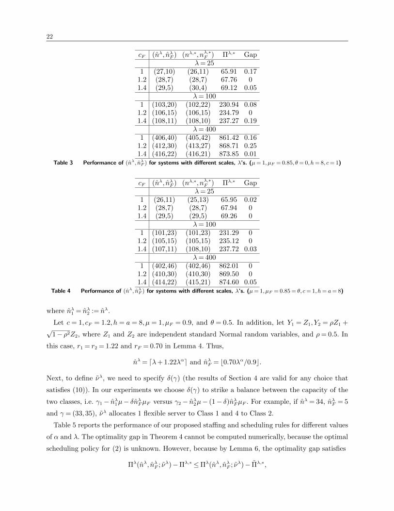
22

cF (nλ, nλF ) (nλ,∗, nλ,∗F ) Πλ,∗ Gapλ= 25

1 (27,10) (26,11) 65.91 0.171.2 (28,7) (28,7) 67.76 01.4 (29,5) (30,4) 69.12 0.05

λ= 1001 (103,20) (102,22) 230.94 0.08

1.2 (106,15) (106,15) 234.79 01.4 (108,11) (108,10) 237.27 0.19

λ= 4001 (406,40) (405,42) 861.42 0.16

1.2 (412,30) (413,27) 868.71 0.251.4 (416,22) (416,21) 873.85 0.01

Table 3 Performance of (nλ, nλF ) for systems with different scales, λ’s. (µ= 1, µF = 0.85, θ= 0, h= 8, c= 1)

cF (nλ, nλF ) (nλ,∗, nλ,∗F ) Πλ,∗ Gapλ= 25

1 (26,11) (25,13) 65.95 0.021.2 (28,7) (28,7) 67.94 01.4 (29,5) (29,5) 69.26 0

λ= 1001 (101,23) (101,23) 231.29 0

1.2 (105,15) (105,15) 235.12 01.4 (107,11) (108,10) 237.72 0.03

λ= 4001 (402,46) (402,46) 862.01 0

1.2 (410,30) (410,30) 869.50 01.4 (414,22) (415,21) 874.60 0.05

Table 4 Performance of (nλ, nλF ) for systems with different scales, λ’s. (µ= 1, µF = 0.85 = θ, c= 1, h= a= 8)

where nλ1 = nλ2 := nλ.

Let c = 1, cF = 1.2, h = a = 8, µ = 1, µF = 0.9, and θ = 0.5. In addition, let Y1 = Z1, Y2 = ρZ1 +√

1− ρ2Z2, where Z1 and Z2 are independent standard Normal random variables, and ρ= 0.5. In

this case, r1 = r2 = 1.22 and rF = 0.70 in Lemma 4. Thus,

nλ = dλ+ 1.22λαe and nλF = b0.70λα/0.9c.

Next, to define νλ, we need to specify δ(γ) (the results of Section 4 are valid for any choice that

satisfies (10)). In our experiments we choose δ(γ) to strike a balance between the capacity of the

two classes, i.e. γ1− nλ1µ− δnλFµF versus γ2− nλ2µ− (1− δ)nλFµF . For example, if nλ = 34, nλF = 5

and γ = (33,35), νλ allocates 1 flexible server to Class 1 and 4 to Class 2.

Table 5 reports the performance of our proposed staffing and scheduling rules for different values

of α and λ. The optimality gap in Theorem 4 cannot be computed numerically, because the optimal

scheduling policy for (2) is unknown. However, because by Lemma 6, the optimality gap satisfies

Πλ(nλ, nλF ; νλ)−Πλ,∗ ≤Πλ(nλ, nλF ; νλ)− Πλ,∗,

23

where Πλ,∗ is the optimal value of (9), we use Πλ(nλ, nλF ; νλ)− Πλ,∗ as an approximation of the

optimality gap. Note that this approximation is larger than the actual optimality gap. We refer to

it as “Approx. Gap” in Table 5.

We observe that for a fixed value of λ, the gap decreases as α increases. For example, when

λ= 25, as α increases from 0.6 to 1, the gap decreases from 9.6 to 4.4. This agrees with the results

in Theorem 4, i.e., the optimality gap is O(λ1−α), which decreases as α increases. For a fixed value

of α, the ratio between the gap and Πλ,∗ decreases as λ increase. For example, when α= 0.8, as λ

increases from 25 to 100, the gap decreases from 5.5% of Πλ,∗ to 2% of Πλ,∗.

λ= 25 λ= 50 λ= 100 λ= 200

α Πλ,∗ Approx. Gap Πλ,∗ Approx. Gap Πλ,∗ Approx. Gap Πλ,∗ Approx. Gap0.6 78.4 9.6 143.0 12.2 265.2 14.7 498.9 18.60.8 104.1 5.7 194.1 6.7 363.9 7.2 685.3 7.91 152.9 4.4 305.8 4.6 611.7 4.5 1223.3 4.2

Table 5 Performance of (nλ, nλF ; νλ) for systems with different values of λ and α.

(c= 1, cF = 1.2, h= a= 8, µ= 1, µF = 0.9, θ= 0.5, ρ= 0.5)

We next compare the pre-limit performance of three asymptotically optimal scheduling policies:

νλ, νλR, and νλI introduced in Section 4.2. We observe in Table 6 that

Πλ(nλ, nλF ; νλI )<Πλ(nλ, nλF ; νλ)<Πλ(nλ, nλF ; νλR).

The performance gaps between νλR and νλI are small in all cases. This demonstrates that using as

crude a policy as νλR still leads to good performances.

λ= 25 λ= 50 λ= 100 λ= 200α νλI νλ νλR νλI νλ νλR νλI νλ νλR νλI νλ νλR

0.6 86.3 88.0 88.3 153.0 155.2 155.5 276.8 279.9 280.3 513.6 517.5 518.10.8 108.3 109.8 110.0 199.5 200.8 201.0 369.2 371.1 371.4 691.2 693.2 693.51 156.2 157.3 157.5 309.6 310.4 310.6 614.3 616.2 616.4 1226.6 1227.5 1227.7

Table 6 The cost under other scheduling policies ν ∈ νλI , νλ, νλR for different values of λ and α.

(c= 1, cF = 1.2, h= a= 8, µ= 1, µF = 0.9, θ= 0.5, ρ= 0.5)

6. Concluding Remarks

In this paper, we study the joint optimal staffing and scheduling problem for a two-class queue

with both dedicated and flexible servers. We quantify how the cost of flexibility affects the optimal

size of the flexible pool. We conclude the paper with some remarks for future research.

24

Non-preemption For the deterministic arrival rate setting, our scheduling policy νλ,∗ is preemp-

tive. For example, we allow a customer in service with the flexible pool to be transferred to the

dedicated pool if a dedicated server becomes available. If we restrict ourselves to non-preemptive

policies, one may be tempted to define a non-preemptive version of the policy, and prove that it

performs asymptotically as well as the preemptive version in the many-server heavy-traffic regime.

Unfortunately, this asymptotic result is unlikely to hold in our case. This is because the size of

the flexible pool, O(√λ), is not large enough to cause instantaneous changes in Xλ in the limit,

which indicates that the non-preemptive version of the policy may not be able to closely ‘track’

the preemptive policy (see Atar (2005) for a similar argument).

For the random arrival rate setting, our scheduling policy νλ is preemptive, but this is not needed

to achieve the optimality gap in Theorem 4. Indeed, a simple coupling argument can show that

a non-preemptive fastest-server-first scheduling policy outperforms the preemptive slowest-server-

first scheduling policy νλR, and the latter is still asymptotically optimal.

Multiple customer classes When there are k customer classes, servers can potentially have 2k−1

different skill sets, i.e., each of the non-empty subsets of 1, · · · , k. In this case, we need to specify

the optimal size of each potential server pool as well as the corresponding scheduling policy. As k

increases, the number of possible system configurations can become very large, posing substantial

analytical challenges.

When facing demand uncertainty, we can still approximate the optimal staffing problem with

a multi-product inventory management problem with demand substitution. Bassamboo et al.

(2010a) study such inventory networks when the ‘staffing’ costs are affine (or convex) in the degree

of flexibility. Let S1, S2 ⊆ 1, · · · , k, and let nSi denote the number of servers with skill set Si. We

also write |Si| for the cardinality of set Si. Bassamboo et al. (2010a) finds that if it is optimal

to set nS1, nS2

> 0 with S1 ( S2, then |S1|= |S2| − 1. This implies that if the optimal sizes of the

dedicated pools are all positive, i.e., ni > 0 for i = 1,2, . . . , k, then the only other server pools

we need to consider are those with skill set i, j, i 6= j, i, j = 1, . . . , k. This can help reduce the

number of possible system configurations that one needs to consider.

Appendix A: Two important stochastic dominance results

In this section, we present two important stochastic dominance results that are useful for our subsequent

analysis, e.g., the proofs of Theorem 1, Lemma 1, and Lemma 3. These results build on coupling arguments

and can be of independent interest.

Let Y (t) = (Y1(t), Y2(t)); t≥ 0 and Y (t) = (Y1(t), Y2(t)); t≥ 0 be two positive recurrent birth-and-death

processes. The birth (arrival) rates are λ for both Yi and Yi, i= 1,2. Let ζi(y) be the death (departure) rate

of Yi when Y (t) = y. We also define ζΣ(y) = ζ1(y) + ζ2(y), ζM(y) = ζ1(y)1y1 ≥ y2+ ζ2(y)1y1 < y2, and

25

ζm(y) = ζ1(y)1y1 ≤ y2+ζ2(y)1y1 > y2. Similarly, let ζi(y) be the death rate of Yi, i= 1,2, when Y (t) = y,

ζΣ(y) = ζ1(y) + ζ2(y), ζM(y) = ζ1(y)1y1 ≥ y2+ ζ2(y)1y1 < y2, and ζm(y) = ζ1(y)1y1 ≤ y2+ ζ2(y)1y1 >

y2.

The following two lemmas provide sufficient conditions to establish stochastic dominance between Y (∞)

and Y (∞).

Lemma 7. For Y (t); t≥ 0 and Y (t); t≥ 0, suppose

P1) ζΣ(y)≥ ζΣ(y) whenever y1 + y2 = y1 + y2 and y1 ∨ y2 ≤ y1 ∨ y2;

P2) ζM(y)≥ ζM(y) whenever y1 ∨ y2 = y1 ∨ y2 and y1 + y2 ≤ y1 + y2.

Then, Y1(∞) +Y2(∞)≤st Y1(∞) + Y2(∞) and Y1(∞)∨Y2(∞)≤st Y1(∞)∨ Y2(∞).

Proof. We prove the lemma by constructing a coupling, under which

Y1(t) +Y2(t)≤ Y1(t) + Y2(t) and Y1(t)∨Y2(t)≤ Y1(t)∨ Y2(t)

for all t≥ 0 path-by-path (Dong et al. 2015).

We start by introducing the coupling. Let Y (0) = Y (0) = y0 for any fixed y0 ∈ N20. We denote the k-th

potential transition time in both systems by tk with t0 = 0. In particular, for Y (tk) = y and Y (tk) = y, let

δM =

e1 y1 ≥ y2

e2 y1 < y2

and δm =

e2 y1 ≥ y2

e1 y1 < y2

.

Similarly let

δM =

e1 y1 ≥ y2

e2 y1 < y2

and δm =

e2 y1 ≥ y2

e1 y1 < y2

.

We then generate tk+1 − tk from an exponential distribution with rate Λ := 2λ + ζΣ(y) ∨ ζΣ(y). We also

generate a random variable U uniformly distributed on [0,1]. We update the states of the two systems

according to the following:

Y (tk+1) = Y (tk) +

δM 0≤U ≤ λ/Λδm λ/Λ<U ≤ 2λ/Λ

−δM 2λ/Λ<U ≤ (2λ+ ζM(y))/Λ

−δm (2λ+ ζM(y))/Λ<U ≤ (2λ+ ζΣ(y))/Λ

0 Otherwise;

and

Y (tk+1) = Y (tk) +

δM 0≤U ≤ λ/Λδm λ/Λ<U ≤ 2λ/Λ

−δM 2λ/Λ<U ≤ (2λ+ ζM(y))/Λ

−δm (2λ+ ζM(y))/Λ<U ≤ (2λ+ ζΣ(y))/Λ

0 Otherwise.

Now, let S = k ∈ N0 : Y1(tk) + Y2(tk) = Y1(tk) + Y2(tk), and let the elements of S, si, be ordered such

that 0 = s0 < s1 < · · · . We will prove by induction that

Y1(tk)∨Y2(tk)≤ Y1(tk)∨ Y2(tk) and Y1(tk) +Y2(tk)≤ Y1(tk) + Y2(tk) for 0≤ k≤ si for any i∈N. (13)

For i= 0, we have Y1(0) +Y2(0) = Y1(0) + Y2(0) and Y1(0)∨Y2(0) = Y1(0)∨ Y2(0) by construction.

26

Suppose (13) holds for some i, i ∈ N0. We first note that for k = si + 1, if si + 1 ∈ S, we have

Y1(tk) + Y2(tk) = Y1(tk) + Y2(tk). If si + 1 /∈ S, then by the coupling construction and P1, there must be

a departure from Y but not Y . Consequently, Y1(tk) + Y2(tk) < Y1(tk) + Y2(tk). This also implies that for

si + 1< k < si+1 (we set si+1 =∞ if si is the last element in S), Y1(tk) + Y2(tk)< Y1(tk) + Y2(tk). We next

note that for si <k≤ si+1, by our coupling construction, if there is an arrival, it either joins the larger queue

in both systems or the smaller queue in both systems. Thus, in this case Y1(tk)∨Y2(tk)≤ Y1(tk)∨ Y2(tk). If

there is a departure, then we further consider two cases.

Case 1. Y1(tk−1)∨Y2(tk−1)< Y1(tk−1)∨ Y2(tk−1): since the difference between the two quantities changes by

at most 1 at each epoch, we have Y1(tk)∨Y2(tk)≤ Y1(tk)∨ Y2(tk).

Case 2. Y1(tk−1) ∨ Y2(tk−1) = Y1(tk−1) ∨ Y2(tk−1): by P2, if there is a departure from the larger queue in

Y , there must be a departure from the larger queue in Y . Moreover, if Y1(tk−1) = Y2(tk−1), as Y1(tk−1) +

Y2(tk−1)≤ Y1(tk−1) + Y2(tk−1), we have Y1(tk−1) = Y2(tk−1). Thus, Y1(tk)∨Y2(tk)≤ Y1(tk)∨ Y2(tk).

Above all, Y1(t) + Y2(t) ≤ Y1(t) + Y2(t) and Y1(t) ∨ Y2(t) ≤ Y1(t) ∨ Y2(t) for all t ≥ 0 under our coupling

construction. This further implies the stochastic dominance results for the stationary distributions.

Lemma 8. For Y (t); t≥ 0 and Y (t); t≥ 0, suppose

P1) ζΣ(y)≤ ζΣ(y) whenever y1 + y2 = y1 + y2 and y1 ∧ y2 ≥ y1 ∧ y2;

P2) ζm(y)≤ ζm(y) whenever y1 ∧ y2 = y1 ∧ y2 and y1 + y2 ≥ y1 + y2.

Then, Y1(∞) +Y2(∞)≥st Y1(∞) + Y2(∞) and Y1(∞)∧Y2(∞)≥st Y1(∞)∧ Y2(∞).

Proof. The coupling construction follows a similar coupling idea as the proof of Lemma 7. We highlight

the difference here for completeness.

Let Y (0) = Y (0) = y0 for any fixed y0 ∈N20. We denote the k-th potential transition time in both systems

by tk with t0 = 0. In particular, for Y (tk) = y and Y (tk) = y, we generate tk+1 − tk from an exponential

distribution with rate Λ := 2λ+ ζΣ(y)∨ ζΣ(y). We also generate a random variable U uniformly distributed

on [0,1] and update the states of the two systems according to the following:

Y (tk+1) = Y (tk) +

δM 0≤U ≤ λ/Λδm λ/Λ<U ≤ 2λ/Λ

−δm 2λ/Λ<U ≤ (2λ+ ζm(y))/Λ

−δM (2λ+ ζm(y))/Λ<U ≤ (2λ+ ζΣ(y))/Λ

0 Otherwise;

and

Y (tk+1) = Y (tk) +

δM 0≤U ≤ λ/Λδm λ/Λ<U ≤ 2λ/Λ

−δm 2λ/Λ<U ≤ (2λ+ ζm(y))/Λ

−δM (2λ+ ζm(y))/Λ<U ≤ (2λ+ ζΣ(y))/Λ

0 Otherwise.

We next prove by contradiction that

Y1(tk)∧Y2(tk)≥ Y1(tk)∧ Y2(tk) and Y1(tk) +Y2(tk)≥ Y1(tk) + Y2(tk) for all k≥ 0. (14)

Let k > 0 be the minimal index such that either (i) Y1(tk)∧Y2(tk)< Y1(tk)∧ Y2(tk) or (ii) Y1(tk)+Y2(tk)<

Y1(tk) + Y2(tk), assuming the existence of such k.

27

In Scenario (i), Y1(tk−1)∧Y2(tk−1) = Y1(tk−1)∧ Y2(tk−1) and Y1(tk−1)+Y2(tk−1)≥ Y1(tk−1)+ Y2(tk−1). If

there is an arrival event at time tk, then based on our coupling construction, this is an arrival to both systems,

and the arrival is either to the smaller queue in both systems or to the large queue in both. If Y1(tk−1) =

Y2(tk−1) so that Y1∧Y2 does not increase at tk, then as Y1(tk−1)+Y2(tk−1)≥ Y1(tk−1)+ Y2(tk−1), Y1(tk−1) =

Y2(tk−1), and so Y1∧ Y2 does not increase either. Hence, in this case Y1(tk)∧Y2(tk) = Y1(tk)∧ Y2(tk). Suppose

instead there is a departure event at tk. There must be a departure from the smaller component in Y .

However, by P2 and our coupling construction, there must be a departure from the smaller component in Y

as well. Hence, we again have that Y1(tk)∧Y2(tk) = Y1(tk)∧ Y2(tk). Thus, Scenario (i) is not feasible.

In Scenario (ii), Y1(tk−1)∧Y2(tk−1)≥ Y1(tk−1)∧ Y2(tk−1) and Y1(tk−1) +Y2(tk−1) = Y1(tk−1) + Y2(tk−1).

Since arrivals coincide in both systems, there must be a departure from Y at tk. However, by P1 and our

coupling construction, there must be a departure from Y as well. This rules out Scenario (ii).

Combining the analysis for the two scenarios, there is a contradiction. Thus, (14) holds, which further

implies the stochastic dominance results for the stationary distributions.

Appendix B: Application of the stochastic dominance results

B.1. Proofs of Lemma 1 and Lemma 3

In this section, we apply Lemma 7 to compare two system configurations. Lemmas 1 and 3 then follow as

corollaries to this comparison.

Fix policy νλ,∗ for Xλ, which has nλ servers in each dedicated server pool and nλF flexible servers. Consider

two auxiliary queueing systems Xλ and Xλ based on Xλ. Xλ has no flexible servers. Each dedicated pool

of Xλ has nλ servers that can work at rate µ and nλF/2 servers that can work at rate µF . When assigning

customers to servers, the rate-µ servers are prioritized. On the other hand, Xλ does not have any dedicated

servers. Instead, it has 2nλ+nλF flexible servers, among which 2nλ servers can work at rate µ and nλF servers

can work at rate µF . When assigning customers to servers, we again prioritize the faster servers.

Lemma 9. Suppose θ≤ µF . For Xλ, Xλ and Xλ, if (nλ, nλF )∈Ωλ(θ),

Xλ1 (∞) + Xλ

2 (∞)≤stXλ1 (∞) +Xλ

2 (∞)≤st Xλ1 (∞) + Xλ

2 (∞);

Xλ1 (∞)∨ Xλ

2 (∞)≤stXλ1 (∞)∨Xλ

2 (∞)≤st Xλ1 (∞)∨ Xλ

2 (∞);(Xλ

1 (∞) + Xλ2 (∞)− 2nλ−nλF

)+ ≤stQλΣ(∞)≤st

(Xλ

1 (∞)−nλ−nλF/2)+

+(Xλ

2 (∞)−nλ−nλF/2)+

.

Proof of Lemma 9. Because all three processes are two-dimensional birth-and-death processes with com-

mon arrival rate λ, we can apply Lemma 7. To simplify the notation, we omit the superscript λ. Set Y =X

and Y = X. Then the death rates take the form:

ζ1(y1, y2) =

µ(y1 ∧n) +µF ((y1−n)+ ∧nF ) + θ(y1−n−nF )+ y1 ≥ y2

µ(y1 ∧n) +µF ((y1−n)+ ∧ (nF − (y2−n)+)+) + θ((y1−n)+− (nF − (y2−n)+)+) y1 < y2

ζ2(y1, y2) =

µ(y2 ∧n) +µF ((y2−n)+ ∧ (nF − (y1−n)+)+) + θ((y2−n)+− (nF − (y1−n)+)+) y1 ≥ y2

µ(y2 ∧n) +µF ((y2−n)+ ∧nF ) + θ(y2−n−nF )+ y1 < y2

ζ1(y1, y2) = µ(y1 ∧n) +µF (nF/2∧ (y1−n)+) + θ(y1−n−nF/2)+

ζ2(y1, y2) = µ(y2 ∧n) +µF (nF/2∧ (y2−n)+) + θ(y2−n−nF/2)+

28

Since µ≥ µF ≥ θ, it is straightforward to verify that P1 and P2 in Lemma 7 hold. Thus, from the proof of

Lemma 7, we can construct a coupling such that

Y1(t) +Y2(t)≤ Y1(t) + Y2(t) and Y1(t)∨Y2(t)≤ Y1(t)∨ Y2(t)

for t≥ 0 path-by-path. In addition,

QΣ(t) =((X1(t)−n)+ + (X2(t)−n)+−nF

)+≤ (X1(t)− (n+nF/2))+ + (X2(t)− (n+nF/2))+

≤ (X1(t)− (n+nF/2))+ + (X2(t)− (n+nF/2))+

As Y is positive recurrent for (n,nF ) ∈Ωλ(θ), so is Y . Sending t to infinity for the coupled processes, we

have the stochastic dominance results in stationarity. The stochastic dominance results for X over X follow

similarly.

For Lemma 1, we note that under the policy νλ,∗, for (nλ, nλF )∈Ωλ(0),

Xλ1 (∞) +Xλ

2 (∞)≤st Xλ1 (∞) + Xλ

2 (∞)

by Lemma 9. Then, the stability of Xλ1 and Xλ

2 implies the stability of (Xλ1 ,X

λ2 ).

For Lemma 3, we have µ= µF . In this case,

QλΣ(∞; 0,2nλ +nλF )

d=(Xλ

1 (∞) + Xλ2 (∞)− 2nλ−nλF

)+.

Then, by Lemma 9, under the policy νλ,∗, we have

QλΣ(∞; 0,2nλ +nλF )≤st Qλ

Σ(∞;nλ, nλF ).

B.2. Proof of Theorem 1

We apply Lemma 7 to prove Theorem 1. To simplify notation, we omit the superscript λ. Consider Y (t) =

X(t;n,nF ;ν∗) and Y (t) =X(t;n,nF ;ν). We will first verify that P1 and P2 in Lemma 7 hold.

For P1, y1 + y2 = y1 + y2 and y1 ∨ y2 ≤ y1 ∨ y2. Since µ≥ µF ≥ θ,

ζΣ(y)≤ ζΣ(y)≤ ζΣ(y).

For P2, y1∨y2 = y1∨ y2 and y1 +y2 ≤ y1 + y2. Without loss of generality, suppose y1 ≥ y2 and y1 = y1 ≥ y2.

Then,

ζM(y)≤ ζM(y) = µ(y1 ∧n) +µF (nF ∧ (y1−n)+) + θ(y1−n−nF )+ = ζM(y).

The positive recurrence of Y is established in Lemma 1. For Y , if it is not positive recurrent, we define

Yi(∞) =∞. Then by Lemma 7,

Xλ1 (∞;n,nF ;ν∗) +Xλ

2 (∞;n,nF ;ν∗)≤stXλ1 (∞;n,nF ;ν) +Xλ

2 (∞;n,nF ;ν)

and

Xλ1 (∞;n,nF ;ν∗)∨Xλ

2 (∞;n,nF ;ν∗)≤stXλ1 (∞;n,nF ;ν)∨Xλ

2 (∞;n,nF ;ν).

Lastly, for the queue length, consider the function f : N20→ N0 defined by f(y1, y2) = ((y1 − n)+ + (y2 −

n)+−nF )+. Note that if y1 + y2 ≤ y1 + y2 and y1 ∨ y2 ≤ y1 ∨ y2, then f(y)≤ f(y). Therefore,

QλΣ(∞;n,nF , ν

∗) =((Xλ

1 (∞;n,nF ;ν∗)−n)+ + (Xλ2 (∞;n,nF ;ν∗)−n)+−nF

)+≤st

((Xλ

1 (∞;n,nF ;ν)−n)+ + (Xλ2 (∞;n,nF ;ν)−n)+−nF

)+ ≤st QλΣ(∞;n,nF ;ν).

29

B.3. Optimal scheduling rule when θ≥ µF = µ

Define φλ,∗ by

Zλi (t) = minnλ,Xλi (t) for i= 1,2; (15)

and if Xλ1 (t)≤Xλ

2 (t),

ZλF1(t) = minnλF , (Xλ1 (t)−nλ)+, ZλF2(t) = minnλF −ZλF1(t), (Xλ

2 (t)−nλ)+; (16)

otherwise,

ZλF1(t) = minnλF −ZλF2(t), (Xλ1 (t)−nλ)+, ZλF2(t) = minnλF , (Xλ

2 (t)−nλ)+. (17)

That is, the flexible pool gives priority to the class with fewer customers in the system. The next theorem

show that φλ,∗ is optimal when θ≥ µF = µ.

Theorem 5. Suppose θ≥ µ= µF . For any deterministic Markovian scheduling policy νλ,

E[QλΣ(∞;nλ, nλF ;νλ)]≥E[Qλ

Σ(∞;nλ, nλF ;φλ,∗)],

which implies that Πλ(nλ, nλF ;νλ)≥Πλ(nλ, nλF ;φλ,∗).

Proof of Theorem 5. The proof of Theorem 5 uses a coupling construction similar to that of Theorem 1,

but does so by considering a ‘dual’ problem where we maximize the number of busy servers. In particular,

the key observation is that

θE[QλΣ(∞)] = 2λ−µE[Zλ1 (∞) +Zλ2 (∞)]−µFE[ZλF (∞)] (18)

so that minimizing E[QλΣ(∞)] is equivalent to maximizing

µE[Zλ1 (∞) +Zλ2 (∞)] +µFE[ZλF (∞)].

This may be accomplished by keeping Xλ1 +Xλ

2 and Xλ1 ∧Xλ

2 both large. Based on this observation, we shall

prove Theorem 5 using Lemma 8.

To simplify the notation, we drop the superscript λ. Let Y (t) =X(t;n,nF ;φ∗) and Y (t) =X(t;n,nF ;ν).

We next verify P1 and P2 of Lemma 8.

For P1, y1 + y2 = y1 + y2 and y1 ∧ y2 ≥ y1 ∧ y2. In this case, we have

ζΣ(y)≤ ζΣ(y)≤ ζΣ(y).

For P2, y1∧y2 = y1∧ y2 and y1 +y2 ≥ y1 + y2. Without loss of generality, suppose y1 ≤ y2 and y1 = y1 ≤ y2.

Then,

ζm(y) = ζ1(y)≥ µ(y1 ∧ (n+nF )) + θ(y1−n−nF )+ = ζm(y)

From Lemma 8, we can construct a coupling, under which

Y1(t) +Y2(t)≥ Y1(t) + Y2(t) and Y1(t)∧Y2(t)≥ Y1(t)∧ Y2(t).

This further implies that

µ(Z1(t) +Z2(t)) +µFZF (t)≥ µ(Z1(t) + Z2(t)) +µF ZF (t).

As θ > 0, both Y and Y are positive recurrent. Thus,

µ(Z1(∞) +Z2(∞)) +µFZF (∞)≥st µ(Z1(∞) + Z2(∞)) +µF ZF (∞),

This completes the proof due to (18).

30

Remark 2. It is hard to extend the results in Theorem 5 to the case where µ> µF . This is because when

µ> µF , P1 in Lemma 8 no longer holds. For example, consider n= nF = 1, y = (1,1) and y = (0,2). In this

case, ζΣ(y) = 2µ> µ+µF ≥ ζΣ(y).

Appendix C: Proofs of the Results in Section 3.2

C.1. Proof of Lemma 2.

Note that E[QλΣ(∞; bRλ +

√Rλc,0)] =O(

√λ) (Garnett et al. 2002). Thus,

Πλ,∗ ≤Πλ(bRλ +√Rλc,0) = 2cRλ +O(

√λ).

To prove Πλ,∗ = 2cRλ +O(√λ), it suffices to prove that nλ,∗ =Rλ +O(

√λ) and nλ,∗F =O(

√λ).

We first prove lim supλ→∞nλ,∗−Rλ√

λ<∞. Suppose by contradiction that there exists a subsequence λkk∈N

such that limk→∞ λk =∞ and limk→∞(nλk,∗−Rk)/√λk =∞, where Rk = λk/µ. Then,

Πλk(nλk,∗, nλk,∗F )− 2cRk√λk

≥ c(2nλk,∗+nλk,∗F − 2Rk)√λk

≥ 2c(nλk,∗−Rk)√λk

→∞,

contradicting that Πλ,∗ ≤ 2cRλ +O(√λ).

We next prove that lim infλ→∞nλ,∗−Rλ√

λ>−∞ and lim supλ→∞

nλ,∗F√λ<∞.

Consider the case where θ = 0. Note that for stability, 2nλ,∗µ+ nλ,∗F µF > 2λ. To prove lim supλ→∞nλ,∗F√λ<

∞, we suppose for contradiction that there exists a subsequence λkk∈N such that limk→∞ λk =∞ and

limk→∞ nλk,∗F /

√λk =∞. Note that 2nλk,∗ > 2λk/µ−nλk,∗F µF/µ. Then,

Πλk(nλk,∗, nλk,∗F )− 2cRk√λk

≥ c(2nλk,∗− 2Rk) + cFnλk,∗F√

λk≥ nλk,∗F (cF − cµF/µ)√

λk→∞,

contradicting that Πλ,∗ ≤ 2cRλ + O(√λ). Since 2nλk,∗ > 2λk/µ − nλk,∗F µF/µ, this also shows that

lim infλ→∞nλ,∗−Rλ√

λ>−∞.

We now turn to the case where θ > 0. We first note that θE[QλΣ(∞;nλ, nλF )] ≥ 2λ − 2nλµ − nλFµF . To

prove lim supλ→∞nλ,∗F√λ<∞, suppose for contradiction that there exists a subsequence λkk∈N such that

limk→∞ λk =∞ and limk→∞ nλk,∗F /

√λk =∞. Note that

Πλk(nλk,∗, nλk,∗F )− 2cRk√λk

≥ 2c(nλk,∗−Rk) + cFnλk,∗F√

λk. (19)

Since the LHS of (19) must be bounded, say by 2cC for some constant C > 0, we have

nλk,∗−Rk ≤C√λk−

cF2cnλk,∗F .

Therefore,

λk−nλk,∗µ≥cFµ

2cnλk,∗F −Cµ

√λk ≥

1

2nλk,∗F µF −Cµ

√λk.

Next, for h/θ+ a= cF/µF + δ = c/µ+ ε satisfying 0< δ < ε,

Πλk(nλk,∗, nλk,∗F )− 2cRk√λk

=(h/θ+ a)θE[Qλ

Σ(∞;nλk,∗, nλk,∗F )] + 2c(nλk,∗−Rk) + cFnλk,∗F√

λk

≥ (h/θ+ a)(2λk− 2nλk,∗µ−nλk,∗F µF ) + 2c(nλk,∗−Rk) + cFnλk,∗F√

λk

=2ε(λk−nλk,∗µ)− δnλk,∗F µF√

λk

≥ (ε− δ)nλk,∗F µF − 2εCµ√λk√

λk→∞

31

as k→∞. This contradicts that Πλ,∗ ≤ 2cRλ +O(√λ), and so nλF =O(

√λ).

To prove that lim infλ→∞nλ,∗−Rλ√

λ>−∞, assume for contradiction that there exists a subsequence λkk∈N

such that limk→∞ λk =∞ and limk→∞(nλk,∗−Rk)/√λk =−∞. Then for nλk,∗F =O(

√λk)

Πλk(nλk,∗, nλk,∗F )− 2cRk√λk

≥ 2ε(λk−nλk,∗µ)− δnλk,∗F µF√λk

=−2εµ(nλk,∗−Rk)− δnλk,∗F µF√

λk→∞.

This is a contradiction.

C.2. Some auxiliary lemmas

Before we prove Theorem 2, we first present three auxiliary lemmas.

Lemma 10. Let Mλ = Mλ(t) : t≥ 0 be a sequence of ergodic Markov chains taking values in Rm, and

h : Rm→Rn be a measurable function. Suppose

1. h(Mλ(t))⇒R(t) in Dn if h(Mλ(0))⇒R(0) as λ→∞, where R is a continuous ergodic process with a

unique stationary distribution R(∞);

2. h(Mλ(∞)) : λ≥ 1 is tight.

Then, h(Mλ(∞))⇒R(∞) as λ→∞.

Proof. The proof follows similar lines of argument as Gamarnik and Zeevi (2006). As (h(Mλ(∞)) : λ≥ 1is tight, every subsequence has a convergent further subsequence. Let Y be a weak limit of (h(Mλ(∞)) :

λ≥ 1, i.e., there exists a sequence λk : k ∈N, such that h(Mλk(∞))⇒ Y as k→∞.

Now for each k, set Mλk(0)d=Mλk(∞). Then, we have Mλk(t)

d=Mλk(∞) for any t≥ 0. This implies that

h(Mλk(0))⇒ Y , which further implies that h(Mλk(t))⇒ R(t) in Dn as k→∞. As R(0)d= Y , R(t)

d= Y .

Furthermore, as R(t)⇒ R(∞) as t→∞, Yd= R(t)

d= R(∞). Therefore, every weak limit of (h(Mλ(∞)) :

λ≥ 1 follows the same distribution as R(∞). This indicates that h(Mλ(∞))⇒R(∞) as λ→∞.

Let Xλ1 (·) denote the number of customers in a system with arrival rate λ, nλ rate-µ servers and nλF/2

rate-µF servers.

Lemma 11. If either (i) θ = 0 and λ < nλµ+nλF2µF = λ+ Θ(

√λ) or (ii) θ > 0, nλµ = λ+O(

√λ), and

nλF =O(√λ),

supλ>1

E

( (Xλ1 (∞)−nλ−nλF/2)+

√λ

)2<∞.

Proof. Let Cλ = nλ +nλF/2. We first note that Xλ1 (·) is a positive-recurrent birth-death process. Let πλ

denote its stationary distribution. In Case (i), for k≥Cλ, we have

πλ(k) = πλ(Cλ)

(λ

nλµ+nλF

2µF

)k−Cλ.

This implies that (Xλ1 (∞)−Cλ)+ is stochastically bounded by a geometric random variable with probability

of success

1− λ

nλµ+nλFµF/2= Θ(1/

√λ).

32

Thus, E[(Xλ

1 (∞)−Cλ)+)2]

=O(λ).

In Case (ii), choose lλ ≥ 0 such that lλ = O(√λ) and nλµ+

nλF2µF + lλθ = λ+ Θ(

√λ), and note that it

suffices to prove that

supλ>1

E

( (Xλ1 (∞)−nλ−nλF/2− lλ)+

√λ

)2<∞.

Let Dλ = nλ +nλF/2 + lλ. For k≥Dλ, we have

πλ(k) = πλ(Dλ)

k−Dλ∏j=1

(λ

nλµ+nλF

2µF + lλθ+ jθ

)≤ πλ(Dλ)

(λ

nλµ+nλF

2µF + lλθ

)k−Dλ.

Thus (Xλ1 (∞)−Dλ)+ is stochastically bounded by a geometric random variable with probability of success

1− λ

nλµ+nλFµF/2 + lλθ= Θ(1/

√λ),

Thus, E[(Xλ

1 (∞)−Dλ)+)2]

=O(λ).

Lemma 12. For (nλ, nλF )∈Ωλ(θ), 2nλ +nλF = 2Rλ + γ√Rλ + o(

√Rλ), and nλF =O(

√λ), we have

supλ>1

E[

(Xλi (∞)−nλ)−√

λ

]<∞.

Proof. We prove the lemma for i= 1 only; the case i= 2 is similar. Let πλ1 (k) = P(Xλ1 (∞) = k). Then for

0≤ k < nλ, we have λπλ1 (k) = (k+ 1)µπλ1 (k+ 1). This implies that

E[(Xλ1 (∞)−nλ)−] = πλ1 (nλ)

nλ∑k=0

(nλ− k)µn

λ−knλ!

λnλ−kk!

≤ 1∑nλ

k=0µnλ−knλ!

λnλ−kk!

·nλ∑k=0

(nλ− k)µn

λ−knλ!

λnλ−kk!

=1∑nλ

k=0µnλ−knλ!

λnλ−kk!

· 1

πλc (nλ)·πλc (nλ)

nλ∑k=0

(nλ− k)µn

λ−knλ!

λnλ−kk!

=1∑nλ

k=0 πλc (k)

·E[(Xλc (∞)−nλ)−]

where Xλc denotes the number-in-system process of an M/M/(nλ + nλF ) + M queue with arrival rate λ

and service rate µ, and abandonment rate θ ≥ 0, and πλc denotes the stationary distribution of Xλc . As

E[(Xλc (∞)− nλ − nλF )−] =O(

√λ) (Garnett et al. 2002) and nλF =O(

√λ), E[(Xλ

c (∞)− nλ)−] =O(√λ). We

also note that∑nλ

k=0 πλc (k) = P(Xλ

c ≤ nλ) = Θ(1). Thus, E[(Xλ1 (∞)−nλ)−] =O(

√λ).

C.3. Proof of Theorem 2

Define, for i= 1,2, the fluid-scale processes

Zλi (t) =Zλi (t)

nλ, Aλi (t) =

Ai(λt)

nλ, and Sλi (t) =

Si(nλµt)

nλ.

We also define, for i= 1,2,

Gλi (t) =

Gi(θ√λt)√λ

and SλFi(t) =SFi(µF

√λt)√

λ.

33

Define, for i= 1,2, the diffusion-scale processes

Aλi (t) =Ai(λt)−λt√

λand Sλi (t) =

Si(nλµt)−nλµt√

λ.

We first note that because

Xλi (t) =Xλ

i (0) +Ai(λt)−Gi

(θ

∫ t

0

Qλi (s)ds

)−Si

(µ

∫ t

0

Zλi (s)ds

)−SFi

(µF

∫ t

0

ZλFi(s)ds

),

we have that

Xλi (t) = Xλ

i (0) + Y λi (t) +Fi(X

λ)(t),

where

Y λi (t) = Aλi (t)− Sλi

(∫ t

0

Zλi (s)ds

)−

SFi(µF∫ t

0ZλFi(s)ds

)√λ

−µF∫ t

0

fi(Xλ(s))ds

−

Gi

(θ∫ t

0Qλi (s)ds

)√λ

− θ∫ t

0

(Xλ(s)+− fi(Xλ(s))ds

+λ−nλµ√

λt

and

Fi(Xλ)(t) = µ

∫ t

0

Xλi (s)− ds− (µF − θ)

∫ t

0

fi(Xλ(s))ds− θ

∫ t

0

Xλi (s)+ ds. (20)

The proof of Theorem 2 is then divided into six steps.

Step 1. Establish the convergence of the fluid-scale number-in-service processes Zλi .

Lemma 13. For (nλ, nλF ) ∈ Ωλ(θ), suppose nλ = Rλ + β√Rλ + o(

√Rλ) and nλF = βF

√Rλ + o(

√Rλ). If

Zλi (0)→ 1, i= 1,2,, then Zλi ⇒ I in D as λ→∞.

Proof of Lemma 13. For any fixed ε > 0 and T > 0, we shall prove that

limλ→∞

P(

inf0≤t≤T

Zλ1 (t)< 1− ε)→ 0.

Define τλ1 = inf0 ≤ t ≤ T : Zλ1 (t) < 1 − ε and τλ2 = sup0 ≤ t < τλ1 : Zλ1 (t) > 1 − ε/2. Let Eλ be

the event that τλ1 and τλ2 are well-defined, i.e. τλi ≤ T . The initial condition Zλi (0) → 1 implies thatinf0≤t≤T Z

λ1 (t)< 1− ε

⊆ Eλ for λ sufficiently large.

As Zλ1 (t)< 1 for t ∈ [τλ2 , τλ1 ], all Class 1 arrivals on [τλ2 , τ

λ1 ] join the dedicated server pool immediately on

arrival. Moreover there are no abandonments from Class 1. Thus,

(Aλ1(τλ1 )− Aλ1(τλ2−))−

(Sλ1

(∫ τλ1

0

Z1(s)ds

)− Sλ1

(∫ τλ2

0

Z1(s)ds

))= Zλ1 (τλ1 )− Zλ1 (τλ2−)≤−ε/2.

This further implies that

P(Eλ)≤ P

inf0≤s≤t≤T

0≤u≤s

(Aλ1(t)− Aλ1(s))− (Sλ1 (u+ t− s)− Sλ1 (u))≤−ε/2

→ 0,

where the convergence follows from the fact that, by the functional strong law of large numbers (FSLLN)

for Poisson processes, (Aλ1 , Sλ1 )⇒ (µχ,µχ) as λ→∞. The analysis for Zλ2 follows similarly.

34

We note from Lemma 13 that in the fluid scale, the dedicated servers are busy all the time.

Step 2. Establish proper limits for the diffusion-scale processes Y λi .

Lemma 14. For (nλ, nλF ) ∈ Ωλ(θ), suppose nλ = Rλ + β√Rλ + o(

√Rλ) and nλF = βF

√Rλ + o(

√Rλ). If

Zλi (0)→ 1, i= 1,2, then(Y λ

1 , Yλ2

)⇒ (√

2B1−β√µχ,√

2B2−β√µχ) in D2 as λ→∞,

where B1 and B2 are independent Brownian motions.

Proof of Lemma 14. Recall that

Y λi (t) = Aλi (t)− Sλi

(∫ t

0

Zλi (s)ds

)−

SFi(µF∫ t

0ZλFi(s)ds

)√λ

−µF∫ t

0

fi(Xλ(s))ds

−

Gi

(θ∫ t

0Qλi (s)ds

)√λ

− θ∫ t

0

(Xλ(s)+− fi(Xλ(s))ds

+λ−nλµ√

λt.

We shall analyze the five components of Yi in sequence.

First, by the functional central limit theorem (FCLT) for Poisson processes, Aλi ⇒ Bi in D as λ→∞,

where Bi is a Brownian motion.

Second, as∫ ·

0Zλi (s)ds⇒ χ (Lemma 13), by a random time change, the FCLT for Poisson processes, and

the continuous mapping theorem (Chapter 13 of Whitt (2002)), we have Sλi(∫ ·

0Zλi (s)ds

)⇒ Bi in D as

λ→∞, where Bi is a Brownian motion and is independent of Bi.

Third, by the FSLLN for Poisson processes, SλFi⇒ µFχ as λ→∞. Next, we rewrite∫ t0ZλFi(s)ds√

λ=

∫ t

0

fλi (Xλ1 (s), Xλ

2 (s))ds,

where

fλ1 (x1, x2) =

x+1 ∧

nλF√λ, x1 ≥ x2,

x+1 ∧

(nλF√λ−x+

2

)+

, x1 <x2;and fλ2 (x1, x2) =

x+2 ∧

(nλF√λ−x+

1

)+

, x1 ≥ x2,

x+2 ∧

nλF√λ, x1 <x2.

Then, as fλ→ f as λ→∞,

SFi

(µF∫ t

0ZλFi(s)ds

)√λ

−µF∫ t

0

fi(Xλ(s))ds

=SλFi

(1√λ

∫ t

0

ZλFi(s)ds

)−µF

∫ t

0

fλi (Xλ(s))ds+µF

∫ t

0

fλi (Xλ(s))− fi(Xλ(s))ds

⇒0 as λ→∞.

Fourth, by the FSLLN for Poisson processes, Gλi → θχ as λ→∞. Then, because

θ∫ t

0Qλi (s)ds√λ

=θ∫ t

0((Xλ

i (s)−nλ)+−ZλFi(s))ds√λ

= θ

∫ t

0

(Xλi (s)+− fλi (Xλ

1 (s), Xλ2 (s))ds,

Gi

(θ∫ t

0Qλi (s)ds

)√λ

− θ∫ t

0

(Xλ(s)+− fi(Xλ(s))ds

=Gλi

(1√λ

∫ t

0

Qλi (s)ds

)− θ√

λ

∫ t

0

Qλi (s)ds+ θ

∫ t

0

(fi(Xλ(s)− fλi (Xλ(s))ds

⇒0 as λ→∞.

35

Fifth, under the assumption of the lemma, (λ−nλµ)/√λ→−β√µ as λ→∞.

Finally, putting the five parts together, we have the result.

Step 3. Establish the C-tightness of the Xλ : λ≥ 1.

Lemma 15. For (nλ, nλF ) ∈ Ωλ(θ), suppose nλ = Rλ + β√Rλ + o(

√Rλ) and nλF = βF

√Rλ + o(

√Rλ). If

Xλ(0)⇒ X(0) as λ→∞,Xλ : λ≥ 1

is C-tight in [0, T ] for all T > 0.

Proof of Lemma 15. Following the C-tightness definition in Chen and Zhang (2000), we will prove that

for any fixed ε, γ > 0, there exist δ > 0 and λ0 > 0 such that for all λ≥ λ0,

P

sup0≤s<t≤T|s−t|<δ

|Xλi (t)− Xλ

i (s)| ≥ ε

≤ γfor i= 1,2. Consider the representation

Xλi (t) =Xλ

i (0) + Aλi (t)− Sλi(∫ t

0

Zλi (s)ds

)+λ−nλµ√

λt+µ

∫ t

0

Xλi (s)− ds

−SFi

(µF∫ t

0ZλFi(s)ds

)√λ

−Gi(θ

∫ t0Qλi (s)ds)

√λ

.

First, as

Xλi (0) + Aλi (t)− Sλi

(∫ t

0

Zλi (s)ds

)+λ−nλµ√

λt⇒ Xi(0) +

√2Bi(t)−β

√µt in D as λ→∞

and√

2Bi(t)− β√µt is continuous, Xλ

i (0) + Aλi (t)− Sλi(∫ t

0Zλi (s)ds

)+ (λ− nλµ)/

√λ : λ ≥ 1 is C-tight

(Lemma 4.2 of Chen and Zhang (2000)).

Second, for 0≤ s≤ t≤ T ,

1√λ

(SFi

(µF

∫ t

0

ZλFi(u)du

)−SFi

(µF

∫ s

0

ZλFi(u)du

))≤SλFi

(∫ s0ZλFi(u)du√λ

+nλF (t− s)√

λ

)− SλFi

(∫ s0ZλFi(u)du√λ

).

Then, the C-tightness of 1√λSFi

(µF∫ ·

0ZλFi(s)ds

) follows from the fact that nλF/

√λ→ βF/

√µ <∞ and

SλFi⇒ µFχ in D as λ→∞.

Third, for 0≤ s≤ t≤ T , we note that

1√λ

(Gi

(θ

∫ t

0

Qλi (u)du

)−Gi

(θ

∫ s

0

Qλi (u)du

))≤Gλ

i

(∫ s0Qλi (u)du+ (t− s) sup0≤v≤T Q

λi (v)

√λ

)− Gλ

i

(∫ s0Qλi (u)du√λ

).

Then, to prove that 1√λGi(θ

∫ ·0Qλi (s)ds) is C-tight, it suffices to prove that for any γ > 0, there exists

K,λ0 > 0, such that P(

sup0≤v≤T Qλi (v)/

√λ≥K

)≤ γ/2 for every λ > λ0. Furthermore, since nλF =O(

√λ),

it is sufficient to prove that P(

sup0≤v≤T Xλi (v)≥K

)≤ γ/2, which follows from Lemma 9.

Fourth, we prove that µ∫ ·

0Xλi (s)− ds : λ≥ 1 is C-tight. For 0≤ s≤ t≤ T , we first note that

µ

∫ t

0

Xλi (u)− du−µ

∫ s

0

Xλi (u)− du≤ µ(t− s) sup

0≤u≤TXλi (u)−.

36

Next from Lemma 12 we have that for any γ > 0, there exists K > 0 and λ0 > 0 such that for all λ> λ0,

P(

sup0≤u≤T

Xλi (u)− >K

)≤ γ.

Thus, µ∫ ·

0Xλi (s)− ds : λ≥ 1 is C-tight.

Putting the four parts together, we have the C-tightness ofXλ : λ≥ 1

.

Lemma 15 implies that any subsequence of Xλ has a weakly convergent further subsequence and the limit

is continuous almost surely (Proposition 4.1 in Chen and Zhang (2000)).

Step 4. Establish that F is continuous at almost all limit points of Xλ.

Lemma 16. For (nλ, nλF ) ∈ Ωλ(θ), suppose nλ =Rλ + β√Rλ + o(

√Rλ) and nλF = βF

√Rλ + o(

√Rλ). The

mapping F :D2→D2 defined in (20) is continuous at almost all limit points of Xλ.

Proof of Lemma 16. From the C-tightness of Xλ : λ ≥ 1, almost all sub-sequential limits of Xλ are

continuous. Thus, it suffices to prove continuity of F under the uniform topology. We denote by X a generic

sub-sequential limit of Xλ.

Fix T > 0. For X ∈D2, define ‖X‖T

= sup0≤t≤T max(|X1(t)|, |X2(t)|). Now, fix ε > 0. Consider X,Y ∈D2

with X continuous and ‖X −Y ‖T< ε/2.

For 0≤ t≤ T , ∣∣∣∣∫ t

0

Xi(s)− ds−

∫ t

0

Yi(s)− ds

∣∣∣∣< εt/2≤ εT/2.Similarly, ∣∣∣∣∫ t

0

Xi(s)+ ds−

∫ t

0

Yi(s)+ ds

∣∣∣∣< εt/2≤ εT/2.Next, for fi, when |X1(t)−X2(t)| ≥ ε, if X1(t)>X2(t), then Y1(t)>Y2(t), and if X1(t)<X2(t), then Y1(t)<

Y2(t). In this case, we have |fi(X(t))−fi(Y (t))| ≤ ε/2. If, instead, |X1(t)−X2(t)|< ε, |fi(X(t))−fi(Y (t))| ≤

βF/√µ. Putting the two cases together, we have∣∣∣∣∫ t

0

fi(X(s))ds−∫ t

0

fi(Y (s))ds

∣∣∣∣≤ ε

2

∫ t

0

1|X1(s)−X2(s)| ≥ εds+βF√µ

∫ t

0

1|X1(s)−X2(s)|< εds

≤εT2

+βF√µ

∫ T

0

1|X1(s)−X2(s)|< εds.

Above all,

|Fi(X)(t)−Fi(Y )(t)| ≤µ∣∣∣∣∫ t

0

Xi(s)− ds−

∫ t

0

Yi(s)− ds

∣∣∣∣+ θ

∣∣∣∣∫ t

0

Xi(s)+ ds−

∫ t

0

Yi(s)+ ds

∣∣∣∣+ (µF − θ)

∣∣∣∣∫ t

0

fi(X(s))ds−∫ t

0

fi(Y (s))ds

∣∣∣∣≤εµT

2+εθT

2+ε(µF − θ)T

2+βF√µ

(µF − θ)∫ T

0

1|X1(t)−X2(t)|< εdt

→ βF√µ

(µF − θ)∫ T

0

1X1(t) =X2(t)dt as ε ↓ 0.

37

This implies that to prove continuity of F at X, it suffices to prove that P(∫ T

01X1(t) = X2(t)dt= 0

)= 1.

Note that Xλ⇒ X implies that X takes the form

Xi(t) = Xi(0) +√

2Bi(t)−β√µt+µ

∫ t

0

Xi(s)− ds+ θ

∫ t

0

Xi(s)+ ds−Li(t),

where Li(t) is a weak limit of (µF − θ)∫ t

0fi(X

λ(s))ds. We also note that Li(t) is monotone increasing

and bounded by (µF − θ)βF t/√µ. Thus, Li has finite total variation. Meanwhile, since X is continuous,∥∥∥X∥∥∥

T<∞. As

∫ t0Xi(s)

− ds≤∫ T

0Xi(s)

− ds <∞, µ∫ t

0Xi(s)

− ds has finite total variation as well. Similarly,

θ∫ t

0Xi(s)

+ ds has finite total variation as well. It then follows that X(t) is the sum of a Brownian motion

and other terms of finite total variation. Therefore X spends almost surely zero time on X1(s) = X2(s)(Turner 2000).

Step 5. Establish that X is suitably well-posed.

The following lemma follows directly from Proposition 5.3.10 in Karatzas and Shreve (1998).

Lemma 17. The diffusion equation

Xi(t) = Xi(0) +√

2Bi(t)−β√µt+µ

∫ t

0

Xi(s)− ds− (µF − θ)

∫ t

0

fi(X(s))ds− θ∫ t

0

Xi(s)+ ds

has a unique (weak) solution.

Steps 1-5 together establish the process level convergence of Xλ, i.e.,

Xλ⇒ X in D2 as λ→∞.

We also note that

QλΣ(t) =

(Xλ

1 (t)+ + Xλ2 (t)+−nλF/

√λ)+

=(Xλ

1 (t)+ + Xλ2 (t)+−βF/

õ)+

+ gλ(Xλ1 (t), Xλ

2 (t))

where ∣∣∣gλ(Xλ1 (t), Xλ

2 (t))∣∣∣= ∣∣∣∣(Xλ

1 (t)+ + Xλ2 (t)+−nλF/

√λ)+

−(Xλ

1 (t)+ + Xλ2 (t)+−βF/

√µ)+∣∣∣∣

≤ |nλF/√λ−βF/

√µ| → 0 as λ→∞.

This implies that QλΣ⇒

(X+

1 + X+2 −βF/

õ)+

in D as λ→∞.

Step 6. Establish the appropriate interchange of limits and uniform integrability results.

Lemma 18. For (β,βF )∈ Ω(θ), the diffusion process X is positive recurrent.

Proof of Lemma 18. We will show that the function V (x1, x2) = 12(x2

1 +x22) is a Lyapunov function. The

generator G of X applied to V is given by

GV (x) =

2∑i=1

xi(−β√µ+µx−i − θx+

i − (µF − θ)fi(x))

for x∈R2.

We first consider the case θ > 0. Because fi is bounded (by βF/√µ), we have that −β√µ+µx−i − θx+

i −(µF − θ)fi(x)≤−1 for all xi > 0 large enough, and −β√µ+ µx−i − θx+

i − (µF − θ)fi(x)≥ 1 for all −xi > 0

large enough. It follows that GV (x)≤−1 for all |x| large enough.

38

Suppose instead θ = 0. If β > 0, −β√µ+ µx−i − µF fi(x)≤−β√µ < 0 for all xi > 0, and −β√µ+ µx−i −µF fi(x)≥ 1 for all −xi > 0 large enough. Thus we may suppose β ≤ 0.

Suppose first both xi are non-negative, with x1 ≥ x2 ≥ 0 (the case x2 > x1 ≥ 0 is similar). Then, if x1 ≥βF/√µ,

GV (x) = x1(−β√µ−µFβF/√µ)−x2β

√µ≤ −x1√

µ(2βµ+βFµF )≤−1

for x1 large enough, since 2βµ+βFµF > 0.

Next, suppose exactly one xi is non-negative, with x1 ≥ 0>x2 (the case x2 ≥ 0>x1 is similar). We have,

if x1 ≥ βF/√µ,

GV (x) = x1(−β√µ−µF fi(x))−µx22−β

√µx2 ≤−

x1õ

(βµ+βFµF )−µx22 ≤−

x1õ

(2βµ+βFµF )−µx22 ≤−1

for |x| large enough, since 2βµ+βFµF > 0. If instead 0≤ x1 <βF/√µ, we have that x1(−β√µ−µF fi(x)) is

bounded, so again GV (x)≤−1 for |x| large enough.

Finally, suppose xi < 0 for i= 1,2. We have

GV (x) =

2∑i=1

xi(−β√µ−µxi)≤−1

for |x| large enough. This completes the proof.

Lemma 18 implies that X(∞) is well defined.

Lemma 19. Suppose nλ =Rλ + β√Rλ + o(

√Rλ) and nλF = βF

√Rλ + o(

√Rλ), with (nλ, nλF ) ∈ Ωλ(θ) and

(β,βF )∈ Ω(θ). Then,

QλΣ(∞)⇒

(X1(∞)+ + X2(∞)+−βF/

õ)+

as λ→∞

and

E[QλΣ(∞)]→E

[(X1(∞)+ + X2(∞)+−βF/

õ)+]

as λ→∞.

Proof of Lemma 19. Note that

supλ>1

E[(Xλi (∞)+)2]

= supλ>1

E

[((Xλ

i (∞)−nλ)+

√λ

)2]

≤ supλ>1

E

(∑2j=1(Xλ

j (∞)−nλ)+

√λ

)2

≤ supλ>1

E

(∑2j=1

((Xλ

j (∞)−nλ−nλF/2)+ +nλF/2)

√λ

)2

≤ supλ>1

4E

( (Xλ1 (∞)−nλ−nλF/2)+ +nλF/2√

λ

)2 by Lemma 9 and Cauchy-Schwarz Inequality

<∞ by Lemma 11.

(21)

In addition,

supλ>1

E[Xλi (∞)−] = sup

λ>1E[

(Xλi (∞)−nλ)−√

λ

]<∞

39

by Lemma 12. Then we have supλ>1 E[|Xλi (∞)|]<∞, i.e., Xλ(∞) : λ> 1 is tight. Thus, Xλ(∞)⇒ X(∞)

as λ→∞ by Lemma 10. By the continuous mapping and converging together theorems, we have QλΣ(∞)⇒(

X1(∞)+ + X2(∞)+−βF/√µ)+

as λ→∞.

Next, the bound in (21) also implies that Xλi (∞)+ : λ > 1 is uniformly integrable. As Qλ

Σ(∞) ≤

Xλ1 (∞)+ + Xλ

2 (∞)+, QλΣ(∞) : λ> 1 is also uniformly integrable. Thus,

E[QλΣ(∞)]→E

[(X1(∞)+ + X2(∞)+−βF/

õ)+]

as λ→∞.

This concludes the proof of Theorem 2.

C.4. Proof of Theorem 3.

We first prove the ‘only if’ part. Let (nλ, nλF ) be asymptotically optimal, and suppose for contradiction that

it is not of the form stated in the theorem. That is, there exists ε > 0 and a subsequence, which we index

again by λ for convenience, satisfying

min(a,b)∈arg minβ,βF

Vp(β,βF )

∣∣∣nλ−Rλ− a√Rλ∣∣∣+ ∣∣∣nλF − b√Rλ∣∣∣√Rλ

> ε

for each λ. This subsequence is asymptotically optimal, and so it follows from the proof of Lemma 2 that

nλF = bλ√Rλ + o(

√Rλ) and nλ =Rλ + aλ

√Rλ + o(

√Rλ)

for some bounded sequences aλ and bλ. Then, there exist finite constants (a, b) /∈ arg minβ,βF Vp(β,βF )

and a subsequence indexed by λ′, such that

aλ′→ a and bλ′→ b as λ′→∞.

For the ease of notation, we re-index this subsequence by λ. As (a, b) /∈ arg minβ,βF Vp(β,βF ), there exists

(β,βF ) such that Vp(β,βF )< Vp(a, b). Define

nλF = βF√Rλ + o(

√Rλ) and nλ =Rλ +β

√Rλ + o(

√Rλ).

Then,

lim supλ→∞

Πλ(nλ, nλF )−Πλ,∗√λ

≥ lim supλ→∞

Πλ(nλ, nλF )−Πλ(nλ, nλF )√λ

= lim supλ→∞

2c(nλ−Rλ) + cFnλF + (h+ aθ)E[Qλ

Σ(∞;nλ, nλF )]− (2c(nλ−Rλ) + cF nλF + (h+ aθ)E[Qλ

Σ(∞; nλ, nλF )])√λ

=Vp(a, b)− Vp(β,βF )> 0

where the last equality follows from Theorem 2, contradicting asymptotic optimality.

It remains to prove the ‘if’ part. From the proof of the ‘only if’ part, the sequence of optimal staffing levels

(nλ,∗, nλ,∗F ) satisfy

nλ,∗F = dλ√Rλ + o(

√Rλ) and nλ,∗ =Rλ + cλ

√Rλ + o(

√Rλ)

40

for some (cλ, dλ)∈ arg minβ,βF Vp(β,βF ). Next, consider any sequence

nλF = bλ√Rλ + o(

√Rλ) and nλ =Rλ + aλ

√Rλ + o(

√Rλ)

where (aλ, bλ)∈ arg minβ,βF Vp(β,βF ). Then,

lim supλ→∞

Πλ(nλ, nλF )−Πλ,∗√λ

= lim supλ→∞

Πλ(nλ, nλF )−Πλ(nλ,∗, nλ,∗F )√λ

= lim supλ→∞

2c(nλ−Rλ) + cFnλF + (h+ aθ)E[Qλ

Σ(∞;nλ, nλF )]−(2c(nλ,∗−Rλ) + cFn

λ,∗F + (h+ aθ)E[Qλ

Σ(∞;nλ,∗, nλ,∗F )])

√λ

(22)

=V ∗p − V ∗p = 0,

where V ∗p = minβ,βF Vp(β,βF ). To see (22), note that by Theorem 2, for any (a, b)∈ arg minβ,βF Vp(β,βF ),

2ca√Rλ + cF b

√Rλ + o(

√Rλ)√

λ+ (h+ aθ)E[Qλ

Σ(∞;a, b)] = V ∗p + o(1).

Then, (22) follows because arg minβ,βF Vp(β,βF ) is finite under Assumption 1.

Appendix D: Proofs of the Results in Section 4

For x, y ∈R and z ≥ 0, define

Kλ(x, y, z) = Πλ

(p1λ+xλα1

µ,p2λ+ yλα2

µ,zλα2

µF

).

D.1. Proof of Lemma 4.

In this case,

Kλ(x, y, z) = c(p1 + p2)Rλ +λα(c

µx+

c

µy+

cFµF

z

)+ cPλ

αE[(

(Y1−x)+ + (Y2− y)+− z)+]

.

In the first case, note that Kλ(x, y, z) is convex and

∇Kλ(q1, q2,0) = λα(

0,0,cFµF− cPP(Y1 > q1 or Y2 > q2)

).

As cFµF− cPP(Y1 > q1 or Y2 > q2)≥ 0, (q1, q2,0) is optimal.

In the second case, we have

∇Kλ(r1, r2, rF ) = (0,0,0).

The optimality of (r1, r2, rF ) follows due to the convexity of Kλ(x, y, z).

D.2. Proof of Lemma 5.

In this case,

Kλ(x, y, z) =c(p1 + p2)Rλ +λα1c

µx+λα2

(c

µy+

cFµF

z

)+ cPλ

α1E[(

(Y1−x)+ +λα2−α1(Y2− y)+−λα2−α1z)+]

.

Let (x∗λ, y∗λ, z∗λ) be the minimizer of Kλ.

41

We first show that x∗λ = q1 + o(1). Note that K∗λ := Πλ,∗ ≤ Kλ(0,0,0) = c(p1 + p2)Rλ + O(λα1). Since

Kλ(x, y, z)≥ c(p1 + p2)Rλ +λα1 cµx, we have that x∗+λ =O(1).

Now suppose for contradiction that there exists a subsequence, indexed by λk, such that either i) x∗λk →−∞

or ii) x∗λk →C ∈R\q1. Note that

Kλ(x, y, z)≥ c(p1 + p2)Rλ +λα1c

µx+λα2

cFµF

z+ cPλα1E[(Y1−x)+−λα2−α1z)+]

= c(p1 + p2)Rλ +λα1c

µx+λα2

cFµF

z+ cPλα1E[(Y1−x−λα2−α1z)+]

= c(p1 + p2)Rλ +λα1c

µ(x+λα2−α1z) + cPλ

α1E[(Y1−x−λα2−α1z)+] +λα2

(cFµF− c

µ

)z. (23)

First suppose that x∗λk →−∞. Since cP > cF/µF > c/µ and K∗λ ≤ c(p1 + p2)Rλ + O(λα1), it follows that

(x∗λ +λα2−α1z∗λ)−

=O(1). This in turn implies that λα2−α1z∗λ→∞, so that λα2

(cFµF− c

µ

)z∗λ grows to infinity

faster than O(λα1). Then, the second and third terms of the last equation (23) will be O(λα1), while the last

is of a larger order. This contradicts that (x∗λ, y∗λ, z∗λ) is optimal.

Consider the second case x∗λ→C ∈R\q1. Note that

Kλ(q1,0,0) = c(p1 + p2)Rλ +λα1f(q1)

where f(x) = cµx+ cPE[(Y1−x)+]. From (23), we have that

Kλ(x∗λ, y∗λ, z∗λ)≥ c(p1 + p2)Rλ +λα1f(x∗λ +λα2−α1z∗λ) +λα2

(cFµF− c

µ

)z∗λ.

Since q1 is uniquely optimal for f and x∗λ → C, we must have λα2−α1z∗λ → q1 − C > 0. But then

λα2

(cFµF− c

µ

)z∗λ 6= o(λα1), contradicting optimality.

This completes the proof that x∗λ = q1 + o(1). Next, we prove that y∗λ and z∗λ are of the appropriate form.

We first show they are O(1). Consider the partial derivatives

∂Kλ

∂y= λα2

(c

µ− cPP[Y2 > y,λ

α1−α2(Y1−x)+ +Y2− y > z])

and∂Kλ

∂z= λα2

(cFµF− cPP[λα1−α2(Y1−x)+ + (Y2− y)+ > z]

).

By optimality, we have

0<c

cPµ= P[Y2 > y

∗λ, λ

α1−α2(Y1−x∗λ)+ +Y2− y∗λ > z∗λ]≤ P[Y2 > y∗λ]

which implies that y∗+λ = O(1). If y∗−λ 6= O(1), then there is a subsequence (re-indexed by λ) such that

y∗λ→−∞, which implies that

1>c

cPµ= P[Y2 > y

∗λ, λ

α1−α2(Y1−x∗λ)+ +Y2− y∗λ > z∗λ] = P[λα1−α2(Y1−x∗λ)+ +Y2− y∗λ > z∗λ] + o(1)

≥ P[Y2 > y∗λ + z∗λ] + o(1).

This in turn implies z∗λ→∞, and in particular z∗λ > 0. But then

P[λα1−α2(Y1−x∗λ)+ +(Y2−y∗λ)+ > z∗λ] = P[Y2 > y∗λ, λ

α1−α2(Y1−x∗λ)+ +Y2−y∗λ > z∗λ]+o(1) =c

cPµ+o(1)<

cFcPµF

42

so that ∂Kλ∂z

(x∗λ, y∗λ, z∗λ)> 0, contradicting optimality. Hence, y∗λ =O(1).

Next, we show z∗λ =O(1). If not, we can obtain a subsequence indexed again by λ such that z∗λ→∞, and

in particular z∗λ > 0. Since y∗λ =O(1) and x∗λ = q1 + o(1), we have

P[λα1−α2(Y1−x∗λ)+ + (Y2− y∗λ)+ > z∗λ] = P[λα1−α2(Y1− q1)+ > z∗λ] + o(1)≤ P[Y1 > q1] + o(1) =c

cPµ+ o(1)

so that ∂Kλ∂z

(x∗λ, y∗λ, z∗λ)> 0 contradicting optimality. Thus z∗λ =O(1).

Finally, we show that y∗λ and z∗λ have the right asymptotics. Suppose n∗2 and n∗F are not of the specified

form. First suppose P(Y1 > q1 or Y2 > q2)> cFcP µF

. Then, there is a subsequence re-indexed by λ such that

x∗λ→ q1, y∗λ→D ∈R and z∗λ→E ≥ 0, where either D 6= l or E 6= lF . Note that

P[Y2 > y∗λ, λ

α1−α2(Y1−x∗λ)+ +Y2− y∗λ > z∗λ] = P[Y2 >D,Y1 > q1 or Y2 >D+E] + o(1)

= P[Y2 >D+E or (Y2 >D,Y1 > q1)] + o(1)

and

P[λα1−α2(Y1−x∗λ)+ + (Y2− y∗λ)+ > z∗λ] = P[Y1 > q1 or Y2 >D+E] + o(1).

By optimality, we must have either (i) the first probability is ccP µ

and the second is cFcP µF

or (ii) the first

probability is ccP µ

, the second is ≤ cFcP µF

and E = 0. Case (i) is ruled out by the uniqueness of l and lF . If (ii),

then D> q2 in order for the second probability to be ≤ cFcP µF

, but D= q2 is necessary for the first probability

to be ccP µ

. This is a contradiction and thus y∗λ = l+ o(1) and z∗λ = lF + o(1).

We now turn to the other case P(Y1 > q1 or Y2 > q2)< cFcP µF

. Using the previous notation, we can again

obtain a subsequence such that either D 6= q2 or E > 0. The case E = 0 and D 6= q2 can be ruled out by our

previous discussion, so suppose E > 0. By optimality, we must have that

P[Y2 >D+E or (Y2 >D,Y1 > q1)] =c

cPµ

and

P[Y1 > q1 or Y2 >D+E] =cFcPµF

.

The second equation ensures D+E < q2. Then, the first probability is at least P(Y2 >D+E)> P(Y2 > q2) =

ccP µ

, a contradiction. This completes the proof.

D.3. Two auxiliary lemmas

Note that for any given arrival rate realization, under the scheduling policy νλ, the two-class queue can

be decomposed into two independent single-class queues with two types of servers: the high-priority rate-µ

servers and the low-priority rate-µF servers. In this section, we study the single-class queue with arrival rate

γ, n high-priority rate-µ servers, nF low-priority rate-µF servers, and abandonment rate θ= µF . To simplify

the notation, we denote by X the steady-state number of customers in the system, Q the steady-state number

of customers waiting in queue, Z the steady-state number of customers in service with rate-µ servers, and

ZF the steady-state number of customers in service with rate-µF servers.

43

Lemma 20. For the single-class queue with two types of servers and θ= µF , there are universal constants

K1,K2,K3 > 0 (i.e. not depending on n,nF or γ), such that

θE[Q]≤ (γ−nµ−nFµF )+ +K1

√γ exp

(−K2

γ(γ−nµ−nFµF )2

)+K3.

Proof of Lemma 20. We start by showing that

E[X] = γ/θ−nµ/θ+n+ (µ− θ)E[(n−X)+]/θ. (24)

Let ξ(x) denote the death rate at state x. When x > n, ξ(x) = xθ + n(µ − θ); when x ≤ n, ξ(x) = xµ =

xθ+x(µ− θ). Equating the birth rate and the death rate in stationarity, we have

γ =E[Xθ+n(µ− θ)− (n−X)+(µ− θ)],

which implies (24).

First, consider the case where γ ≥ nµ+nFµF . We have

E[Q] = E[(X −n−nF )+]

=E[X]−n−nF +

n+nF−1∑x=0

P[X ≤ x]

= γ/θ−nµ/θ+n+ (µ− θ)E[(n−X)+]/θ−n−nF +

n+nF−1∑x=0

P[X ≤ x] by (24)

= (γ/θ−nµ/θ−nF ) +µ− θθ

n−1∑x=0

P[X ≤ x] +

n+nF−1∑x=0

P[X ≤ x].

It suffices to bound∑n+nF−1

x=0 P[X ≤ x]. Let M1 = bγ/θ− nµ/θ + nc, which is the mode of X (to see this,

note that the death rate ξ(x) is increasing in x, and that the birth rate γ is larger than the death rate

for x < M1, and is smaller than the death rate for x > M1). We then have M1 ≥ n + nF , and ξ(M1) =

nµ+ bγ/θ−nµ/θcθ≤ γ. For 0<k≤M1−n+ 1, note that

P[X =M1− k] = P[X =M1] · ξ(M1)(ξ(M1)− θ) · · · (ξ(M1)− (k− 1)θ)

γk

≤ P[X =M1] · γ(γ− θ) · · · (γ− (k− 1)θ)

γk

= P[X =M1] · 1(1− θ/γ) · · · (1− (k− 1)θ/γ)

≤ P[X =M1] · (1− (k− 1)θ/2γ)k

≤ P[X =M1] · exp(−(k− 1)kθ/2γ) as 1−x≤ exp(−x).

Similarly, for M1−n+ 1<k≤M1,

P[X =M1− k]

=P[X =M1] · 1

γkξ(M1)(ξ(M1)− θ) · · · (ξ(M1)− (M1−n)θ) · (ξ(M1)− (M1−n)θ−µ)

· · · (ξ(M1)− (M1−n)θ− (k−M1 +n− 1)µ)

≤P[X =M1] · ξ(M1)(ξ(M1)− θ) · · · (ξ(M1)− (M1−n)θ) · (ξ(M1)− (M1−n+ 1)θ) · · · (ξ(M1)− (k− 1)θ)

γk

≤P[X =M1] · (1− (k− 1)θ/2γ)k

≤P[X =M1] · exp(−(k− 1)kθ/2γ).

44

Choose A1 > 0 such that A1k2 ≤ k(k− 1)θ/2 for all k≥ 2, then for any 1<k≤M1

P[X =M1− k]≤ P[X =M1] · exp(−A1k

2/γ).

Next, we bound P[X =M1]. Note that for k > 0,

P[X =M1 + k] = P[X =M1] · γk

(ξ(M1) + θ) · · · (ξ(M1) + kθ).

Then, because

γb√γc

(ξ(M1) + θ) · · · (ξ(M1) + b√γcθ)≥ γb

√γc

(γ+ θ) · · · (γ+ b√γcθ)

≥ γb√γc

(γ+ b√γcθ)b√γc

=

(1−

b√γcθγ+ b√γcθ

)b√γc≥(

1−b√γcθγ

)b√γc→ exp(−θ) as γ→∞,

for γ large enough and 1≤ k≤ b√γc,

P[X =M1 + k]≥ P[X =M1] · exp(−θ)/2.

Thus, for γ large enough,

1≥M1+b√γc∑k=M1

P[X = k]≥ P[X =M1] · (1 + b√γc exp(−θ)/2)

which implies that

P[X =M1]≤ 1

1 + b√γc exp(−θ)/2≤ B1√

γ,

where B1 = 2 exp(θ).

Above all, we have proven that for γ large enough, when 1<k≤M1,

P[X =M1− k]≤B1 · exp(−A1k

2/γ)/√γ.

Then, for 1<k≤ n+nF ,

P[X ≤ n+nF − k] = P[X ≤M1− (M1−n−nF + k)]

=

M1∑j=M1−n−nF+k

P[X =M1− j]

≤M1∑

j=M1−n−nF+k

B1 exp(−A1j

2/γ)/√γ

≤∫ ∞M1−n−nF+k−1

B1 exp(−A1j

2/γ)/√γ dj

≤ B1

√2π

2√A1

exp(−A1(M1−n−nF + k− 1)2/(2γ)

)by Chernoff-Cramer bound.

Choose D1 > 0 such that D1x2 ≤A1(x− 1)2/2 for all x≥ 2. Then, for γ large enough, and 2≤ k≤ n+nF ,

P[X ≤ n+nF − k]≤C1 exp(−D1(M −n−nF + k)2/γ

)

45

where C1 = B1

√2π

2√A1

.

Finally, we have for γ large enough

n+nF−1∑x=0

P[X ≤ x]≤∫ n+nF

0

P[X ≤ n+nF −x]dx

≤∫ n+nF

2

P[X ≤ n+nF −x]dx+ 2

≤∫ n+nF

0

C1 exp(−D1(M1−n−nF +x)2/γ

)dx+ 2

=

∫ M1

M1−n−nF

C1 exp(−D1x

2/γ)dx+ 2

≤ C1

√2πγ

2√D1

exp(−D1(M1−n−nF )2/(2γ)

)+ 2.

Since M1−n−nF =⌊γ−nµ−nF µF

θ

⌋, this completes the proof for γ > nµ+nFµF .

Next, consider the case where nµ≤ γ < nµ+ nFµF . Let M2 = n+ b γ−nµθc be the mode of X in this

case. Note that

n+nF −M2 ≥nµ+nFµF − γ

θ.

Thus, for any C > 0,

exp(−Cθ2(n+nF −M2)2

)≤ exp

(−C(nµ+nFµF − γ)2

).

Next, note that

E[Q] = E[(X −n−nF )+] =

∞∑x=n+nF

P[X >x].

As ξ(M2) = nµ+ b γ−nµθcθ, we have for k > 0,

P[X =M2 + k] = P[X =M2] · γk

(ξ(M2) + θ) · · · (ξ(M2) + kθ)

≤ P[X =M2] · γk

γ(γ+ θ) · · · (γ+ (k− 1)θ)

≤ P[X =M2] ·(

γ

γ+ (k− 1)θ/2

)k/2= P[X =M2] ·

(1− (k− 1)θ/2

γ+ (k− 1)θ/2

)k/2≤ P[X =M2] · exp

(− k(k− 1)θ/4

γ+ (k− 1)θ/2

)≤ P[X =M2] ·

(exp

(−k(k− 1)θ/4

2γ

)+ exp

(−k(k− 1)θ/4

(k− 1)θ

))= P[X =M2] ·

(exp

(−k(k− 1)θ

8γ

)+ exp(−k/4)

).

The last inequality comes from the fact that k(k−1)θ/4

γ+(k−1)θ/2≥ k(k−1)θ/4

2γif γ ≥ (k−1)θ/2 and k(k−1)θ/4

γ+(k−1)θ/2≥ k(k−1)θ/4

(k−1)θ

otherwise. Thus, for all k > 0,

P[X ≥M2 + k] =

∞∑j=k

P[X =M2 + j]

46

≤∞∑j=k

P[X =M2] ·(

exp

(−j(j− 1)θ

8γ

)+ exp (−j/4)

)≤ P[X =M2] ·

(∫ ∞k−1

exp

(−j(j− 1)θ

8γ

)dj+

exp(−k/4)

1− exp(−1/4)

).

Choose B2 > 0 such that B2x2 ≤ x(x− 1)θ/8 for all x≥ 2, and choose F2 > 0 such that F2x

2 ≤B2(x− 1)2/2

for all x ≥ 3. Also, choose A2 > 0 such that P[X = M2] ≤ A2/√γ (the existence of A2 follows similarly to

before.) Then, for all k≥ 3,

P[X ≥M2 + k]≤ P[X =M2] ·(∫ ∞

k−1

exp

(−j(j− 1)θ

8γ

)dj+

exp(−k/4)

1− exp(−1/4)

)≤ A2√

γ

(∫ ∞k−1

exp(−B2j

2/γ)dj+

exp(−k/4)

1− exp(−1/4)

)≤ A2

√2π

2√B2

· exp(−B2(k− 1)2/2γ

)+C2 exp(−D2k)/

√γ

≤E2 exp(−F2k

2/γ)

+C2 exp(−D2k)/√γ

for some universal C2,D2,E2 > 0. Finally,

∞∑x=n+nF

P[X >x] =

∫ ∞n+nF−M2

P[X >M2 +x]dx

≤ 3 +

∫ ∞n+nF−M2+3

E2 exp(−F2x

2/γ)

+C2 exp(−D2x)/√γ dx

≤ 3 +

∫ ∞n+nF−M2

E2 exp(−F2x

2/γ)

+C2 exp(−D2x)/√γ dx

≤ 3 +L2

√γ exp

(−F2(n+nF −M2)2/2γ

)+G2 exp(−D2(n+nF −M2))/

√γ

≤L2

√γ exp

(−F2(n+nF −M2)2/2γ

)+ 3 +G2

for some universal L2,G2 > 0.

Lastly, consider the case where 0 < γ < nµ. This is very similar to the proof of the case nµ ≤ γ <

nµ+ nFµF , but we include it here for completeness. Let M3 = bγ/µc be the mode of X in this case. Note

that

n+nF −M3 ≥nµ+nFµ− γ

µ≥ nµ+nFµF − γ

µ.

Thus, for any C > 0,

exp(−Cµ2(n+nF −M3)2

)≤ exp

(−C(nµ+nFµF − γ)2

).

Next, note that

E[Q] = E[(X −n−nF )+] =

∞∑x=n+nF

P[X >x].

For ξ(M3) = bγ/µcµ, we have for 0<k≤ n−M3,

P[X =M3 + k] = P[X =M3] · γk

(ξ(M3) +µ) · · · (ξ(M3) + kµ),

47

and for k > n−M3,

P[X =M3 + k]

=P[X =M3] · γk

(ξ(M3) +µ) · · · (ξ(M3) + (n−M3)µ)(ξ(M3) + (n−M3)µ+ θ) · · · (ξ(M3) + (n−M3)µ+ (k−n+M3)θ)

≤P[X =M3] · γk

(ξ(M3) +µ) · · · (ξ(M3) + kµ).

Thus, for all k > 0, we have

P[X =M3 + k]≤ P[X =M3] · γk

(ξ(M3) +µ) · · · (ξ(M3) + kµ)

≤ P[X =M3] · γk

γ(γ+µ) · · · (γ+ (k− 1)µ)

≤ P[X =M3] ·(

γ

γ+ (k− 1)µ/2

)k/2= P[X =M3] ·

(1− (k− 1)µ/2

γ+ (k− 1)µ/2

)k/2≤ P[X =M3] · exp

(− k(k− 1)µ/4

γ+ (k− 1)µ/2

)≤ P[X =M3] ·

(exp

(−k(k− 1)µ/4

2γ

)+ exp

(−k(k− 1)µ/4

(k− 1)µ

))= P[X =M3] ·

(exp

(−k(k− 1)µ

8γ

)+ exp(−k/4)

).

The last inequality comes from the fact that k(k−1)µ/4

γ+(k−1)µ/2≥ k(k−1)µ/4

2γif γ ≥ (k − 1)µ/2 and k(k−1)µ/4

γ+(k−1)µ/2≥

k(k−1)µ/4

(k−1)µotherwise. Thus, for all k > 0,

P[X ≥M3 + k] =

∞∑j=k

P[X =M3 + j]

≤∞∑j=k

P[X =M3] ·(

exp

(−j(j− 1)µ

8γ

)+ exp (−j/4)

)≤ P[X =M3] ·

(∫ ∞k−1

exp

(−j(j− 1)µ

8γ

)dj+

exp(−k/4)

1− exp(−1/4)

).

Choose B3 > 0 such that B3x2 ≤ x(x− 1)µ/8 for all x≥ 2, and choose F3 > 0 such that F3x

2 ≤B3(x− 1)2/2

for all x≥ 3. Also, choose A3 > 0 such that P[X =M3]≤A3/√γ. Then, for all k≥ 3,

P[X ≥M3 + k]≤ P[X =M3] ·(∫ ∞

k−1

exp

(−j(j− 1)µ

8γ

)dj+

exp(−k/4)

1− exp(−1/4)

)≤ A3√

γ

(∫ ∞k−1

exp(−B3j

2/γ)dj+

exp(−k/4)

1− exp(−1/4)

)≤ A3

√2π

2√B3

· exp(−B3(k− 1)2/2γ

)+C3 exp(−D3k)/

√γ

≤E3 exp(−F3k

2/γ)

+C3 exp(−D3k)/√γ

for some universal C3,D3,E3 > 0. Finally,

∞∑x=n+nF

P[X >x] =

∫ ∞n+nF−M3

P[X >M3 +x]dx

48

≤ 3 +

∫ ∞n+nF−M3+3

E3 exp(−F3x

2/γ)

+C3 exp(−D3x)/√γ dx

≤ 3 +

∫ ∞n+nF−M3

E3 exp(−F3x

2/γ)

+C3 exp(−D3x)/√γ dx

≤ 3 +L3

√γ exp

(−F3(n+nF −M3)2/2γ

)+G3 exp(−D3(n+nF −M3))/

√γ

≤L3

√γ exp

(−F3(n+nF −M3)2/2γ

)+ 3 +G3

for some universal L3,G3 > 0. This completes the proof.

Next, consider two single-class queues, A and B, with common arrival rate λ and abandonment rate θ.

System A has m high priority rate-µ servers and mF low priority rate-µF servers, while system B has m/r

high priority rate-rµ servers and mF/r low priority rate-rµF servers, for some r > 1. Let QA(∞) and QB(∞)

denote the stationary queue lengths of the two systems respectively.

Lemma 21. For systems A and B,

QA(∞)≤st QB(∞).

Proof of Lemma 21. The proof follows the same lines of argument as the proof of Lemma 2 in Bassamboo

et al. (2010b), and is only included for completeness. Let XA(t) and XB(t) denote the headcount processes,

which are birth-death processes. Let α=m+mF and β = (m+mF )/r be the number of servers in the two

systems, and let ξA(·) and ξB(·) denote the death rates.

We first note that the two systems have the same birth rates. For x≥ 0, ξA(α+ x) = ξB(β + x), and for

0≤ x≤ β, ξA(α−x)≥ ξB(β−x). Initialize XA(0) = α, XB(0) = β. Couple the two systems such that (i) the

arrivals to both systems coincide, and (ii) the departures in system B is a subset of the departures in system

A. Then, for all t≥ 0, XA(t)−α≤XB(t)−β and

QA(t) = (XA(t)−α)+ ≤ (XB(t)−β)+ =QB(t).

As the stationary distribution is well-defined, we have the stochastic dominance of the stationary distribution.

D.4. Proof of Lemma 6

To simplify the notation, we drop the superscript λ and the ‘(∞)’. In particular, let Xi denote the stationary

number of Class i customers in the system, QΣ denote the stationary total queue length, Zi denote the

stationary number of Class i customers served by the dedicated servers, and ZFi denote the stationary

number of Class i customers served by the flexible servers.

We first prove the lower bound. Consider the case where θ ≤ µF . Note that QΣ ≥ f(X1,X2) :=

((X1−n1)+ + (X2−n2)+−nF )+. As f is convex, by Jensen’s inequality

E[QΣ|Λ = γ;ν]≥E[f(X1,X2)|Λ = γ;ν]≥ f(E[X1|Λ = γ;ν],E[X2|Λ = γ;ν]).

Thus,

θE[QΣ|Λ = γ;ν]≥(θE[X1|Λ = γ;ν]− θn1)+ + (θE[X2|Λ = γ;ν]− θn2)+− θnF

)+.

Equating the arrival and departure rates in stationarity, we have

γi = θE[Xi|Λ = γ;ν] + (µ− θ)E[Zi|Λ = γ;ν] + (µF − θ)E[ZFi|Λ = γ;ν].

49

Because E[Zi|Λ = γ;ν]≤ ni and E[ZF1|Λ = γ;ν] +E[ZF2|Λ = γ;ν]≤ nF , for some α= α(γ)∈ [0,1],

γ1 ≤ θE[X1|Λ = γ;ν] + (µ− θ)n1 +α(µF − θ)nF

and

γ2 ≤ θE[X2|Λ = γ;ν] + (µ− θ)n2 + (1−α)(µF − θ)nF .

Then,

θE[QΣ|Λ = γ;ν]≥(θE[X1|Λ = γ;ν]− θn1)+ + (θE[X2|Λ = γ;ν]− θn2)+− θnF

)+≥((γ1−µn1−α(µF − θ)nF )+ + (γ2−µn2− (1−α)(µF − θ)nF )+− θnF

)+≥((γ1−µn1)+ + (γ2−µn2)+−µFnF

)+,

where the last inequality follows from the fact that ((a− c)+ + (b− d)+− e)+ ≥ (a+ + b+− (c+ d+ e))+ for

any c, d, e≥ 0.

Next, consider the case where θ > µF . Note that

θE[QΣ|Λ = γ;ν] = γ1 + γ2−µE[Z1 +Z2|Λ = γ;ν]−µFE[ZF1 +ZF1|Λ = γ;ν].

Consider an auxiliary system, X, with all parameters the same except that its abandonment rate is θ= µF .

We next construct a scheduling policy ν′ such that

E[Z1 +Z2|Λ = γ;ν] = E[Z1 + Z2|Λ = γ;ν′] and E[ZF1 +ZF2|Λ = γ;ν] = E[ZF1 + ZF2|Λ = γ;ν′]. (25)

The policy for ν′ is constructed through a coupling that keeps Zi = Zi and ZFi = ZFi at all times. This

can be achieved by assuming that arrivals and service completions in both systems coincide, and that the

abandonments in the auxiliary system is a subset of the abandonments in the original system since θ < θ.

From (25), we have

θE[QΣ|Λ = γ;ν] = θE[QΣ|Λ = γ;ν′]≥((γ1−µn1)+ + (γ2−µn2)+−µFnF

)+,

where the last inequality follows from our analysis of the case where θ≤ µF .

We next prove the upper bound. We first consider the case when θ= µF . By Lemma 20, we have

θE[QΣ|Λ = γ; ν]

=θE[Q1|Λ = γ; ν] + θE[Q2|Λ = γ; ν]

≤(γ1−µn1−bδnF cµF )+ +K1

√γ

1exp

(−K2

γ1

(γ1−µn1−bδnF cµF )2

)+K3

+ (γ2−µn2−d(1− δ)nF eµF )+ +K1

√γ

2exp

(−K2

γ2

(γ2−µn2−d(1− δ)nF eµF )2

)+K3

≤(γ1−µn1− δnFµF )+ +K1

√γ

1exp

(−K2

γ1

(γ1−µn1−bδnF cµF )2

)+K3 +µF

+ (γ2−µn2− (1− δ)nFµF )+ +K1

√γ

2exp

(−K2

γ2

(γ2−µn2−d(1− δ)nF eµF )2

)+K3 +µF

=((γ1−µn1)+ + (γ2−µn2)+−µFnF )+ + 2(K3 +µF )

+K1

√γ

1exp

(−K2

γ1

(γ1−µn1−bδnF cµF )2

)+K1

√γ

2exp

(−K2

γ2

(γ2−µn2−d(1− δ)nF eµF )2

).

50

The result then follows using the proof of Lemma 1 in Bassamboo et al. (2010b).

Next, consider the case when θ < µF . Let the original system be labeled I. We form an auxiliary system II

with the same parameters, except that the abandonment rate is θII = µF and the holding cost is hII = hµF/θ.

We write

ΠI(n1, n2, nF ; ν) = c(n1 +n2) + cFnF + (a+h/θ)AI(n1, n2, nF ; ν)

where AI(n1, n2, nF ; ν) = θE[QIΣ(n1, n2, nF ; ν)] is the stationary abandonment rate in system I. Similarly,

ΠII(n1, n2, nF ; ν) = c(n1 +n2) + cFnF + (a+h/θ)AII(n1, n2, nF ; ν).

We next show that

AI(n1, n2, nF ; ν)≤AII(n1, n2, nF ; ν). (26)

Note that

Ai =EΛ[Λ−µZi−µFZiF ]

where Zi and ZiF are the stationary number of busy rate-µ servers and rate-µF servers respectively, in system

i, i = I, II. Thus, we only need to show that ZI ≥st ZII and ZIF ≥st ZIIF . Based on the scheduling policy

ν, it suffices to verify the following: If XI is the stationary headcount in a single-class queue with m high

priority rate-µ servers, mF low priority rate-µF servers, and abandonment rate θ, and XII is the same but

with abandonment rate µF , then XI ≥st XII . This is true because the birth rates of the two corresponding

processes are the same, while the death rate in II is higher than in I. This proves (26), which further implies

that

Πλ,I(nλ1 , nλ2 , n

λF ; νλ)≤Πλ,II(nλ1 , n

λ2 , n

λF ; νλ)≤ Πλ(nλ1 , n

λ2 , n

λF ) +O(λ1−α2) as θII = µF .

Lastly, consider the case where θ > µF . We form a new auxiliary system III with the same parameters as

X, except that µIIIF = θ, µIII = µθ/µF , cIII = cθ/µF , and cIIIF = cF θ/µF . Then,

Πλ,I(nλ1 , nλ2 , n

λF ; νλ)≤Πλ,III

(µFθnλ1 ,

µFθnλ2 ,

µFθnλF ; νλ

)by Lemma 21

≤ Πλ(nλ1 , nλ2 , n

λF ) +O(λ1−α2) as µIIIF = θ.

D.5. Proof of Theorem 4.

Let (nλ,∗1 , nλ,∗2 , nλ,∗F ;νλ,∗) be optimal for (2). We have

Πλ(dnλ,∗1 e, dnλ,∗2 e, bn

λ,∗F c; νλ)

≤Πλ(dnλ,∗1 e, dnλ,∗2 e, bn

λ,∗F c) +O(λ1−α2) by the upper bound in Lemma 6

≤Πλ(nλ,∗1 , nλ,∗2 , nλ,∗F ) + 2c+ cPµF +O(λ1−α2)

≤Πλ(nλ,∗1 , nλ,∗2 , nλ,∗F ) +O(λ1−α2)

≤Πλ(nλ,∗1 , nλ,∗2 , nλ,∗F ;νλ,∗) +O(λ1−α2) by the lower bound in Lemma 6.

51

References

Andradottir, Sigrun, Hayriye Ayhan, Douglas G Down. 2003. Dynamic server allocation for queueing net-

works with flexible servers. Operations Research 51(6) 952–968.

Armony, Mor, Avishai Mandelbaum. 2011. Routing and Staffing in Large-Scale Service Systems: The Case

of Homogeneous Impatient Customers and Heterogeneous Servers. Operations Research 59(1) 50–65.

Atar, Rami. 2005. Scheduling control for queueing systems with many servers: Asymptotic optimality in

heavy traffic. The Annals of Applied Probability 15(4) 2606–2650.

Bassamboo, Achal, J. Michael Harrison, Assaf Zeevi. 2006. Design and Control of a Large Call Center:

Asymptotic Analysis of an LP-Based Method. Operations Research 54(3) 419–435.

Bassamboo, Achal, Ramandeep S. Randhawa, Jan A. Van Mieghem. 2012. A Little Flexibility Is All You

Need: On the Asymptotic Value of Flexible Capacity in Parallel Queuing Systems. Operations Research

60(6) 1423–1435.

Bassamboo, Achal, Ramandeep S. Randhawa, Jan A. Van Mieghem. 2010a. Optimal Flexibility Configu-

rations in Newsvendor Networks: Going Beyond Chaining and Pairing. Management Science 56(8)

1285–1303.

Bassamboo, Achal, Ramandeep S. Randhawa, Assaf Zeevi. 2010b. Capacity Sizing Under Parameter Uncer-

tainty: Safety Staffing Principles Revisited. Management Science 56(10) 1668–1686.

Bassamboo, Achal, Assaf Zeevi. 2009. On a data-driven method for staffing large call centers. Operations

Research 57(3) 714–726.

Bertsimas, Dimitris, Xuan Vinh Doan. 2010. Robust and data-driven approaches to call centers. European

Journal of Operational Research 207(2) 1072–1085.

Best, Thomas J, Burhaneddin Sandıkcı, Donald D Eisenstein, David O Meltzer. 2015. Managing hospi-

tal inpatient bed capacity through partitioning care into focused wings. Manufacturing & Service

Operations Management 17(2) 157–176.

Borst, Sem, Avi Mandelbaum, Martin I. Reiman. 2004. Dimensioning Large Call Centers. Operations

Research 52(1) 17–34.

Chen, Hong, Hanqin Zhang. 2000. Diffusion Approximations for Some Multiclass Queueing Networks with

FIFO Service Disciplines. Mathematics of Operations Research 25(4) 679–707.

Dai, J. G., Wuqin Lin. 2008. Asymptotic optimality of maximum pressure policies in stochastic processing

networks. The Annals of Applied Probability 18(6) 2239–2299.

Dai, J. G., Tolga Tezcan. 2011. State Space Collapse in Many-Server Diffusion Limits of Parallel Server

Systems. Mathematics of Operations Research 36(2) 271–320.

Dong, Jing, Pnina Feldman, Galit B. Yom-Tov. 2015. Service Systems with Slowdowns: Potential Failures

and Proposed Solutions. Operations Research 63(2) 305–324.

52

Ernst, Ricardo, Panagiotis Kouvelis. 1999. The Effects of Selling Packaged Goods on Inventory Decisions.

Management Science 45(8) 1142–1155.

Gamarnik, David, Assaf Zeevi. 2006. Validity of heavy traffic steady-state approximations in generalized

Jackson networks. The Annals of Applied Probability 16(1) 56–90.

Gans, Noah, Ger Koole, Avishai Mandelbaum. 2003. Telephone call centers: Tutorial, review, and research

prospects. Manufacturing & Service Operations Management 5(2) 79–141.

Garnett, O., A. Mandelbaum, M. Reiman. 2002. Designing a Call Center with Impatient Customers. Man-

ufacturing & Service Operations Management 4(3) 208–227.

Gurvich, Itai, James Luedtke, Tolga Tezcan. 2010. Staffing Call Centers with Uncertain Demand Forecasts:

A Chance-Constrained Optimization Approach. Management Science 56(7) 1093–1115.

Gurvich, Itay, Ward Whitt. 2009a. Queue-and-Idleness-Ratio Controls in Many-Server Service Systems.

Mathematics of Operations Research 34(2) 363–396.

Gurvich, Itay, Ward Whitt. 2009b. Service-Level Differentiation in Many-Server Service Systems via Queue-

Ratio Routing. Operations Research 58(2) 316–328.

Halfin, Shlomo, Ward Whitt. 1981. Heavy-Traffic Limits for Queues with Many Exponential Servers. Oper-

ations Research 29(3) 567–588.

Harrison, J. Michael, Assaf Zeevi. 2004. Dynamic Scheduling of a Multiclass Queue in the Halfin-Whitt

Heavy Traffic Regime. Operations Research 52(2) 243–257.

Harrison, J. Michael, Assaf Zeevi. 2005. A Method for Staffing Large Call Centers Based on Stochastic Fluid

Models. Manufacturing & Service Operations Management 7(1) 20–36.

Karatzas, Ioannis, Steven Shreve. 1998. Brownian Motion and Stochastic Calculus. 2nd ed. Graduate Texts

in Mathematics, Springer-Verlag, New York.

Kim, Jeunghyun, Ramandeep S Randhawa, Amy R Ward. 2018. Dynamic scheduling in a many-server, mul-

ticlass system: The role of customer impatience in large systems. Manufacturing & Service Operations

Management 20(2) 285–301.

Kocaga, Yasar Levent, Mor Armony, Amy R. Ward. 2015. Staffing Call Centers with Uncertain Arrival Rates

and Co-sourcing. Production and Operations Management 24(7) 1101–1117.

Mandelbaum, Avishai, Sergey Zeltyn. 2009. Staffing Many-Server Queues with Impatient Customers: Con-

straint Satisfaction in Call Centers. Operations Research 57(5) 1189–1205.

Netessine, Serguei, Nils Rudi. 2003. Centralized and Competitive Inventory Models with Demand Substitu-

tion. Operations Research 51(2) 329–335.

Pashler, Harold. 1994. Dual-task interference in simple tasks: data and theory. Psychological bulletin 116(2)

220.

53

Rajaram, Kumar, Christopher S. Tang. 2001. The impact of product substitution on retail merchandising.

European Journal of Operational Research 135(3) 582–601.

Shi, Cong, Yehua Wei, Yuan Zhong. 2019. Process flexibility for multiperiod production systems. Operations

Research 67(5) 1300–1320.

Simchi-Levi, David, Yehua Wei. 2012. Understanding the Performance of the Long Chain and Sparse Designs

in Process Flexibility. Operations Research 60(5) 1125–1141.

Song, Hummy, Anita L. Tucker, Ryan Graue, Sarah Moravick, Julius J. Yang. 2019. Capacity Pooling in

Hospitals: The Hidden Consequences of Off-Service Placement. Management Science 66(9) 3825–3842.

Tezcan, Tolga, JG Dai. 2010. Dynamic control of n-systems with many servers: Asymptotic optimality of a

static priority policy in heavy traffic. Operations Research 58(1) 94–110.

Tsitsiklis, John N., Kuang Xu. 2012. On the power of (even a little) resource pooling. Stochastic Systems

2(1) 1–66.

Turner, Stephen R. E. 2000. A join the shorter queue model in heavy traffic. Journal of Applied Probability

37(1) 212–223.

Van Mieghem, Jan A., Nils Rudi. 2002. Newsvendor Networks: Inventory Management and Capacity Invest-

ment with Discretionary Activities. Manufacturing & Service Operations Management 4(4) 313–335.

Wallace, Rodney B., Ward Whitt. 2005. A Staffing Algorithm for Call Centers with Skill-Based Routing.

Manufacturing & Service Operations Management 7(4) 276–294.

Whitt, Ward. 2002. Stochastic-Process Limits: An Introduction to Stochastic-Process Limits and Their

Application to Queues. Springer Series in Operations Research and Financial Engineering, Springer-

Verlag, New York.

Whitt, Ward. 2006. Staffing a Call Center with Uncertain Arrival Rate and Absenteeism. Production and

Operations Management 15(1) 88–102.