managerial discretion and the economic determinants of the ...dn75/doron nissim - managerial...

Abstract This study investigates the determinants of the expected stock-price volatility assumption that firms use in estimating ESO values and thusoption expense. We find that, consistent with the guidance of FAS 123, firmsuse both historical and implied volatility in deriving the expected volatilityparameter. We also find, however, that the importance of each of the twovariables in explaining disclosed volatility relates inversely to their values,which results in a reduction in expected volatility and thus option value. Thiscan be interpreted as managers opportunistically use the discretion in esti-mating expected volatility afforded by FAS 123. Consistent with this, we findthat managerial incentives or ability to understate option value play a key rolein this behavior. Since discretion in estimating expected volatility is commonto both FAS 123 and 123(R), our analysis has important implications formarket participants as well as regulators.

Keywords Executive stock options Æ Forward-looking information ÆSFAS No. 123 Æ Implied volatility

JEL Classifications M41 Æ J33 Æ G30 Æ G13

E. Bartov (&)Leonard N. Stern School of Business, New York University, 44 W. 4th St., Suite 10-96,New York, NY 10012, USAe-mail: [email protected]

P. MohanramColumbia Business School, Columbia University, 605-A Uris Hall, New York,NY 10027, USAe-mail: [email protected]

D. NissimColumbia Business School, Columbia University, 604 Uris Hall, New York, NY 10027, USAe-mail: [email protected]

123

Rev Acc StudDOI 10.1007/s11142-006-9024-x

Managerial discretion and the economic determinantsof the disclosed volatility parameter for valuing ESOs

Eli Bartov Æ Partha Mohanram Æ Doron Nissim

� Springer Science+Business Media, LLC 2007

Under Statement of Financial Accounting Standards (SFAS) No. 123, firmsare required to disclose the estimated fair value of stock options granted toemployees (ESOs) and pro forma earnings as if ESO cost was recognized inthe income statement. For many firms, especially firms in industries with highoption granting intensity, the effect of ESO cost on earnings is quite signifi-cant. A recent Standard & Poor’s (S&P) survey indicates that mean earningsof all S&P 500 firms would have been lower by 8.6 percent and 7.4 percent in2003 and 2004, respectively, if ESO costs had been recognized. Mr. DavidBlitzer, managing director and chairman of the Index Committee at Standard& Poor’s, observed, ‘‘A change of 7 percent or 8 percent in estimated earningsfor the S&P 500 is significant, especially if investors are not fully aware ofwhat caused the change.’’1

To estimate the fair value of option grants, firms have to select a valuationmodel and estimate relevant parameters, such as expected stock price vola-tility and option life. Given the large impact of ESO costs on earnings and theleeway that firms possess in valuing options, prior research has investigatedwhether managers use this discretion opportunistically to understate optionvalues. For example, Murphy (1996) and Baker (1999) find that in preparingproxy statements’ disclosures, firms opportunistically select the option valu-ation method (fair value versus potential realizable value) to reduce perceivedmanagerial compensation. Further, Yermack (1998) finds that firms ‘‘unilat-erally apply discounts to the Black–Scholes formula,’’ and both Yermack(1998) and Aboody, Barth, and Kaszik (2006) show that firms shortenexpected lives of options to lower option expense. Somewhat surprisingly,however, related research examining whether firms understate expected vol-atility, a critical parameter in option valuation whose estimation is subject toconsiderable discretion under SFAS 123, finds mixed results: Balsam, Mozesand Newman (2003) find no evidence of manipulation of expected volatility;Hodder, Mayew, McAnally, and Weaver (2006) find that managerial incen-tives for opportunistic reporting do not uniformly induce selection of expectedvolatility that understates reported fair values, and Aboody et al. (2006) findmarginally significant evidence of the lowering of expected volatility, ascompared with strong evidence of the lowering of expected option life.

In this paper, we complement this related research that considers allparameters in option valuation, by focusing on the volatility assumption aloneand examining it in depth. We focus on volatility for the following threereasons. First, the volatility assumption is by far the most important input inoption valuation. Brenner and Subrahmanyam (1994), among others, dem-onstrate this result and further show that for options whose strike price equalsthe forward stock price, option value is proportional to volatility (i.e., ifexpected volatility is lowered by 10 percent from 30 percent to 27 percent,option value will also decline by 10 percent). Second, estimating expected

1 See CFO.com, Today in Finance for April 01, 2004, The Cost of Expensing Stock Options, athttp://www.cfo.com/article.cfm/3012993?f=TodayInFinance040104

E. Bartov et al.

123

volatility involves substantial discretion, as SFAS No. 123 states that thestarting point for estimating expected volatility should be historical volatility,but adjustments should be made if ‘‘unadjusted historical experience is arelatively poor predictor of future experience’’ (Para. 276). This contrasts withthe risk free rate, where FASB guidance leaves little room for managerialdiscretion (see Para. 19 of SFAS No. 123), and with the dividend yield, wherea substantial portion of firms offering ESOs pay no dividends and thus set thedividend yield to zero.2 Finally, the somewhat surprising mixed results ofrelated research on whether companies understate expected volatility dis-cussed above may imply that the manipulation of the volatility assumption, ifit indeed occurs, may be more sophisticated or more nuanced, requiring amore detailed investigation.

Using a new approach and a relatively large sample (9,185 firm-years) thatspans a relatively long period (1996–2004), this study investigates the deter-minants of disclosed volatility by asking two questions. The first examines theextent to which companies follow the guidance of SFAS No. 123 and useforward-looking information, in addition to historical volatility, in estimatingexpected volatility. More importantly, the second question examines thecross-sectional variation in the tendency of firms to incorporate such infor-mation. In particular, are firms more likely to incorporate forward-lookinginformation when it implies lower expected volatility and hence smalleroption value? Further, is such opportunism more likely when managerialincentives to understate volatility are greater (e.g., option grants are relativelylarge) or when corporate governance and capital market scrutiny are lax?

Examining these questions requires a measure that captures forward-looking expected volatility information. For companies with traded call or putoptions, one such measure, advocated by the newly promulgated SFAS No.123(R), is the implied stock price volatility of traded options.3 In an efficientcapital market, this measure should reflect both historical and forward-lookinginformation. Thus, the incremental relationship between disclosed andimplied volatilities, after controlling for historical volatility, should indicatethe extent to which disclosed volatility contains forward-looking expectedvolatility information.

The primary innovation in this paper is that we evaluate disclosed volatilityusing two benchmarks: historical volatility and implied volatility. Since SFASNo. 123(R), the successor of SFAS No. 123, explicitly advocates using impliedvolatility in addition to historical volatility (see, Appendix A, Para. A32), this

2 Estimating option lives does involve discretion, but the effect of this assumption on option fairvalue as well as the cross-sectional and time-series variation in expected option lives are relativelysmall. Moreover, there is no obvious benchmark against which this variable can be assessed.3 SFAS No. 123(R), which was promulgated in December, 2004, mandates income statementrecognition for employee stock option expense for fiscal years starting after June 15, 2005.However, in April 2005, the Securities Exchange Commission amended Rule S-X to delay theeffective date for compliance with SFAS No. 123(R) to fiscal year starting after June 15, 2005.Based on the amended rule, most companies are required to adopt SFAS No. 123(R) on January1, 2006.

Managerial discretion and the economic determinants of the disclosed volatility parameter

123

approach allows us to assess whether companies estimated expected volatilityduring the SFAS No. 123 period in a way consistent with the more specificguidance of SFAS No. 123(R).4 Perhaps more importantly, our analysis alsosheds light on whether companies exploit discretion common to the guidancein both SFAS Nos. 123 and 123(R) to lower disclosed volatility and thus theoption expense by opportunistically shifting the weights from one factor toanother. In contrast, related research assesses disclosed volatility indirectly byexamining the difference between reported ESO fair value and a benchmarkvalue produced by the researchers (Hodder et al., 2006), and by studying therelation between incentives and opportunities to understate assumptions andoption values (Aboody et al., 2006). As this research has not used impliedvolatility, it is unable to provide insights regarding the efficacy of the guidancein SFAS Nos. 123 and 123(R) for estimating expected volatility.

We find that disclosed volatility is incrementally related to both historicalvolatility and implied volatility. This appears to indicate that managers areliterally following the dictum in SFAS No. 123 that they ought to incorporateboth historical and forward-looking information in the estimation of expectedvolatility. Further investigation, however, demonstrates that the weights onthe two volatility measures vary inversely to their relative values. For exam-ple, when historical volatility is high relative to implied volatility, the weighton historical volatility, 0.230, is substantially lower than that on implied vol-atility, 0.498. In contrast, when historical volatility is low relative to impliedvolatility, the weight on historical volatility increases nearly four fold to 0.718,whereas the weight on implied volatility decreases to 0.042. These results areconsistent with managers using the discretion afforded by SFAS No. 123 toopportunistically underreport option value.

There are, however, two alternative explanations for these findings. First,managers may place lower weights on higher values of volatility because theyare more likely to contain large measurement error. Results from additionaltests, however, indicate that the opportunistic-behavior explanation is incre-mental to this alternative explanation. Second, while in general SFAS No. 123requires the volatility estimate to be unbiased, Para. 275 of the pronounce-ment guides that if a range of volatility estimates of equal quality are avail-able, ‘‘it is appropriate to use an estimate at the low end of the range ....’’ It isthus arguable that if implied volatility and historical volatility are of equalquality, firms appropriately pick the lower of the two as the volatility estimate.Inconsistent with this alternative explanation, however, we find that theobserved shift in weights between historical and implied volatility is related tothe strength of managerial incentives and ability to understate option value.

These results imply that companies use the discretion afforded by SFASNo. 123 opportunistically to understate volatility and thus lower optionexpense, particularly when their incentives to report lower option expense are

4 SFAS No. 123 guides that in estimating expected volatility companies should consider historicalvolatility and forward-looking information. SFAS No. 123(R) is more specific in that it guides thatin addition to historical volatility, implied volatility from traded options can be considered.

E. Bartov et al.

123

strong. Since the discretion in estimating disclosed volatility is common toboth SFAS Nos. 123 and 123(R), this behavior is likely to increase as optionexpensing starts to directly affect the income statement under SFAS No.123(R), as opposed to the pro-forma disclosure that most firms providedunder SFAS No. 123.

Our analysis has important implications for regulators, investors, andauditors. First, by documenting the widespread usage of implied volatility inthe SFAS No. 123 period, we provide support for the new specific guidance inSFAS No. 123(R), which advocates considering implied volatility, in additionto historical volatility, in estimating expected volatility. However, by showingthat companies shifted the weights between historical and implied volatilityopportunistically, our analysis questions the FASB approach of giving sub-stantial discretion to companies as to how to use these two factors. Moregenerally, our findings have ramifications for standard setters, as they indicatethat when managers are given the alternative of choosing between multiplesources of information, they often use their discretion opportunistically. Oneapproach for restraining this behavior could be requiring firms to justify thechoice of information sources used (or not used) in exercising the discretion attheir disposal. Second, by identifying variables indicating which companies arelikely to act opportunistically in estimating expected volatility and by docu-menting how this opportunistic behavior works (i.e., shifting weights betweenhistorical and implied volatilities) our analysis can help investors and auditorsto detect such companies and correct distortions in disclosed volatility andoption expense.

The remainder of the paper is organized as follows. Section 1 develops theempirical tests. Section 2 delineates the sample selection procedure, definesthe variables, and describes the data. Section 3 presents the empirical findings,and Sect. 4 concludes.

1 Development of the empirical tests

1.1 Primary tests

Our first research question is whether firms follow the guidance in SFAS No.123 and use both historical and forward-looking information in derivingexpected volatility. To address this question, we estimate the followingregression:

rD ¼ aindu; year þ b1rH þ b2r

I þ e; ð1Þ

where the dependent variable, rD, is the volatility assumption used by the firmin calculating the value of option grants, disclosed in Form 10-K; aindu,year

represents an industry-year fixed effect for pooled regressions, and industryeffect for yearly regressions; rH is historical stock-price volatility, calculatedusing monthly returns for the period which ends on the balance sheet date and


123

is equal to the disclosed expected life of the stock options; rI is impliedvolatility, calculated using the prices of traded call and put options as of theend of the fiscal year (more details regarding the measurement of impliedvolatility are provided in the next section).

Implied volatility, which is derived from option prices, reflects both historicaland forward-looking information relevant for the prediction of future stock-price volatility. Consequently, the incremental relationship between disclosedand implied volatilities, after controlling for historical volatility, should indicatethe extent to which disclosed volatility contains forward-looking information. Infact, if implied volatility fully reflects the information in historical volatility andfirms select the volatility assumption with no bias or error, then disclosed vol-atility should be unrelated to historical volatility after considering impliedvolatility. However, implied volatility is not likely to fully reflect the informationin historical volatility. Research in finance finds that while implied volatilityforecasts future volatility better than historical volatility, both measures containinformation incremental to each other (e.g., Mayhew, 1995). This is due to bothmarket inefficiencies in pricing options and errors in option valuation modelsused to derive implied volatility (e.g., the simplifying assumption of continuousprice movements). In the context of ESOs, the advantage of implied volatilityover historical volatility may be smaller as the maturity of ESOs is considerablylonger than that of traded options, from which implied volatility is derived. Still,implied volatility reflects both historical and forward-looking informationrelevant for the prediction of future stock-price volatility.

In terms of Eq. (1), if firms incorporate both historical and forward-lookinginformation in estimating expected volatility, then H1: b1 > 0 and b2 > 0. Incontrast, if they use only historical volatility, then H2: b1 = 1 and b2 = 0. Inaddition, the relative magnitudes of b1 and b2 indicate the extent to whichfirms adjust historical volatility to reflect forward-looking information whenderiving the expected volatility parameter.

Our second research question asks whether firms use forward-lookinginformation opportunistically to lower expected volatility and thus optionvalue. To address this question, we estimate the following model:

rD ¼ aindu; year þ b1rH þ b2r

I þ b3HI IMP

þ b4HI IMP� rH þ b5HI IMP� rI þ e; ð2Þ

where HI_IMP is an indicator variable that equals one when rI > rH (i.e.,when forward-looking information indicates larger expected volatility thanhistorical information), and the other variables are defined as before. In termsof Eq. (2), opportunistic managerial behavior implies that H3: b4 > 0 and b5 < 0.A negative b5 means that the weight on forward-looking informationdecreases when reliance on forward-looking information leads to higherdisclosed volatility and thus larger option expense. An extreme version ofopportunism, where managers rely on forward-looking information solely toreduce disclosed volatility, predicts b2 + b5 = 0; i.e. if implied volatility is

E. Bartov et al.

123

larger than historical volatility, it has no effect on disclosed volatility and thusoption expense.

1.2 Tests of alternative explanations

It is arguable that a relatively high volatility value is associated with highmeasurement error. To distinguish between this measurement-error expla-nation and the opportunistic-behavior interpretation, we replicate Eq. (2)using two alternative dependent variables: realized volatility, rR, and thedifference between realized and disclosed volatilities, rD – rR. Specifically, weestimate the following two models:

rR ¼ a0indu; year þ b01rH þ b02r

I þ b03HI IMPþ b04HI IMP� rH

þ b05HI IMP� rI þ eð3Þ

rD � rR ¼ a�indu; year þ b�1rH þ b�2r

I þ b�3HI IMPþ b�4HI IMP� rH

þ b�5HI IMP� rI þ eð4Þ

where the explanatory variables are defined as in Eq. (2), and rR is realizedvolatility during the period corresponding to the expected life of the stockoptions or up to December 2005, whichever is shorter. We calculate realizedvolatility using monthly stock returns where at least 24 months of returns areavailable and using daily returns otherwise.

Considering rRan unbiased proxy for expected volatility, the parameterestimates from Eq. (3) offer a benchmark against which the estimates fromEq. (2) may be assessed. Specifically, in the absence of opportunistic behavior,the estimates from Eqs. (2) and (3) should be similar, as the measurementerror explanation applies equally to both equations. Conversely, if managerialopportunism plays a role in the determination of rD, then b4 (b5) from Eq. (2)should be greater (smaller) than that from Eq. (3), as the predictions ofpositive b4 and negative b5 due to opportunistic behavior apply only toEq. (2). Note that Eq. (4) is derived by subtracting Eq. (3) fromEq. (2). We can thus formulate the tests distinguishing between the twoexplanations—measurement error and opportunistic behavior—in terms ofEq. (4). That is, the opportunistic-behavior explanation predicts that b�4[0and b�5\0, whereas absence of opportunism implies that b�4 ¼ 0 and b�5 ¼ 0.

A second possible alternative explanation for the predictions of H3 may bethat managers follow Para. 275 of SFAS No. 123, which directs that if multiplevolatility estimates of equal quality are available, the lowest estimate shouldbe used. To assess this alternative explanation, we study the relation betweenmanagerial incentives and ability to understate expected volatility and theopportunistic use of forward-looking volatility information. If managersincorporate forward-looking information opportunistically, they are likely todo so especially when their incentives and ability to understate the optionexpense are strong. More specifically, in terms of Eq. (2), hypothesis H4


123

predicts that b4 (b5) will be increasing (decreasing) in a firm’s incentives and/or ability to understate the option expense. Conversely, if the estimate forexpected volatility reflects the effect of Para. 275, b4 and b5 should be unre-lated to incentives or ability to manipulate the option expense.5

To investigate H4, we re-estimate Eq. (2) for subsamples partitioned basedon various proxies for incentives and ability to understate the option expense,as well as on the interaction between the two effects. If the weights on his-torical and implied volatilities reflect opportunistic behavior rather than therequirement of Para. 275, then bHigh

4 [bLow4 and bHigh

5 \bLow5 , where bHigh

i

represents parameter estimates from subsamples of high incentives/ability tounderstate disclosed volatility and bLow

i represents estimates fromlow-incentives/ability subsamples.

2 Data

2.1 Data sources and sample selection

Our sample covers the nine years from 1996 to 2004. Our sample periodcommences in 1996 because this is the first year companies were required toprovide a (footnote) description of their employee option plans in annualreports and Form 10-K. Our sample period ends in 2004 because this is the lastyear with available data. The sample is generated, as described in Table 1, byintersecting five data sources: the New Constructs database, the source fordisclosed volatilities and annual option grants; the Optionmetrics database,the source of implied volatility; the CRSP database, the source for stockreturns used to compute historical and realized volatilities; the Compustatdatabase, the source for firm characteristics; and the IBES database, thesource of the number of analyst following a firm.6 This procedure yielded asample size of 9,189 firm-years (2,215 distinct firms). However, four firm-yearsare obvious multivariate outliers: they each have v2 value (a measure of thestandardized distance from the other observations, see Watson, 1990) that is atleast 25 percent larger than that of any other observation, while none of theother observations has a v2 that is more than 10 percent larger than the nexthighest v2.7 We thus removed these four firm-years, and our final sampleconsists of 9,185 firm-years (2,215 distinct firms).

5 A necessary condition for the magnitude of volatility understatement to vary with incentives isthat managers incur costs that offset the benefits of reporting understated option expense. Wediscuss these costs in Section 3 below.6 The use of the IBES database did not lead to any loss in sample size. There were 700 obser-vations out of 9,185 with no analyst following data on IBES, which we coded as having zeroanalyst following. Removing these observations does not affect the results reported in Table 7below for either the analyst following partition or the composite measure.7 Following Watson (1990), we detect multivariate outlier observations using the statisticv2

i ¼ ðmi � �mÞ0S�1ðm � �mÞ, where i denotes the ith observation; bar denotes average over allsample firms; m is the 4 · 1 vector of volatilities (historical, implied, disclosed and realized); and Sis the 4 · 4 sample covariance matrix of m.

E. Bartov et al.

123

We next describe how we obtain the volatility measures and other variablesused in our analysis. Companies disclose information about option grants toall employees in the annual report and Form 10-K. These disclosures areprepared according to SFAS No. 123, with value estimates typically based onthe Black–Scholes (1973) methodology.8 We retrieve the stock price volatilityassumption and annual option grants data from the New Constructs database,a machine readable database that gleans stock option compensation data fromForm 10-K footnote disclosures, with an emphasis on Russell 3,000 companiesand recent years (2000 onwards).

Both historical and realized volatility are calculated using monthly stockreturns over a period equal to the expected option life, as disclosed in Form10-K. The period for historical (realized) volatility ends (starts) on the balancesheet date. For example, if the fiscal year end is December 2000 and expectedoption life is three years, historical volatility is measured over the three-yearperiod January 1998 to December 2000, while realized volatility is estimatedover the three-year period January 2001 to December 2003. If the estimationperiod for realized volatility is less than 24 months, we use daily instead ofmonthly returns (a minimum of 50 daily returns is required).

We calculate our measure of implied volatility by using data from theOptionmetrics database and applying the following procedure. First, for eachfirm-year and each strike price, we obtain the implied volatilities of call andput options with the longest maturity as of the end of the fiscal year. Weconsider both calls and puts to mitigate any measurement error in impliedvolatility induced by the Black–Scholes method. We focus on options with the

Table 1 Sample selection procedure

Firm-Years

DistinctFirms

Data on option grants obtained from New Constructs database 16,987 3,025

LESS implied volatility unavailable on Optionmetrics database 6,503 593

Both option grant and implied volatility information available 10,484 2,432

LESS Unavailable CRSP returns to calculate historical/realized volatility 798 215

Option grant, implied volatility and CRSP returns available 9,286 2,227

LESS Unavailable COMPUSTAT information for incentive variables 97 12

Option, volatility, CRSP and COMPUSTAT information all available 9,189 2,215

LESS Deletion of outliers 4 0

FINAL SAMPLE 9,185 2,215

8 It is well recognized that ESOs violate important assumptions underlying the Black–Scholesmodel (e.g., Black–Scholes assume a diffusion process and values European calls, whereas inreality stock prices may jump and nearly all ESOs are American calls). Moreover, academicresearch offers models which might be more appropriate for valuing ESOs (see, e.g., Hemmer,Matsunaga and Shevlin, 1994; Carpenter, 1998). Yet, most firms use the Black–Scholes model tovalue their ESOs, perhaps due to the robustness of the Black–Scholes values and the complexity ofalternative models.


123

longest maturities because employee stock options have very long expectedmaturities (3.31 years on average for our sample firms).9 For both calls andputs, we then identify the options with the strike price closest to the prevailingstock price on both sides, because prior research has demonstrated that near-the-money options perform better in predicting future volatility than deep in-or out-of-the-money options (see, e.g., Hull, 2000; Mayhew, 1995). If an exactmatch is found, we use that option to measure the implied volatility of thecorresponding type (call or put). If not, we extrapolate from the impliedvolatilities of the two options, assigning weights that are inversely propor-tional to the distance between the stock price and the exercise price.10 Finally,we calculate the average of the call and put implied volatilities.

In addition to the four volatility variables (disclosed, historical, implied andrealized), we compute proxies for incentives and ability to understate dis-closed volatility in order to test alternative interpretations of our results. Weuse three proxies for incentives: annual option grants, option holdings, andcapital market issuance. We obtain option data from the New Constructsdatabase. Following Richardson and Sloan (2003), we measure capital marketissuance as the sum of external financing raised from equity, short term debtand long term debt (change in Compustat #60 – #172 + change in #9 + changein #34 + change in #130), scaled by total assets. We also compute three proxiesfor managerial ability to manipulate disclosed volatility: analyst following,institutional ownership, and board independence. Analyst following is mea-sured as the number of analysts issuing one-year ahead EPS forecasts at thefiscal year end (from IBES). Institutional ownership is measured as the per-centage of shares outstanding owned by institutional shareholders at fiscalyear end (from Thomson financial). Board independence is measured as theproportion of board directors that were deemed as independent and withoutany interlocking relationships with any other board members (from theInvestor Responsibility Research Center (IRRC) database).

2.2 Descriptive statistics

Table 2 outlines characteristics of our sample firms (Panel A), as well as thetime (Panel B) and industry (Panel C) distributions of the sample. As evidentfrom the statistics displayed in Panel A, a number of important firm charac-teristics vary substantially across our sample firms. For example, the spread inmarket value of equity—5th percentile of $173 million; $1,452 million mean;95th percentile of $25,985 million—indicates that our sample consists of small,medium, and large firms, and the spread in return on assets between the 5thpercentile(–23.5 percent) and 95th percentile (16.7 percent) suggests that the

9 Indeed, our success in matching on time-to-maturity is only partial. The mean time-to-maturityof our traded options is 329.2 calendar days.10 For example, if stock price is $42 and the two nearest call options have strike prices of $40 and$45 and implied volatilities of 0.34 and 0.36, respectively, we estimate the implied volatility of calloptions as: ð1=2Þ�0:34þð1=3Þ�0:36

ð1=2Þþð1=3Þ ¼ 0:348. If all strike prices are on one side of the prevailing stockprice, we use the implied volatility of the option with the nearest strike price.

E. Bartov et al.

123

Table 2 Sample descriptive statistics

Panel A: Descriptive statistics for sample firm-years (beginning of year)

N Mean Std. Dev. P5 Q1 Median Q3 P95 Sales ($millions) 9,170 4,221 11,880 34 286 993 3,388 18,570

Assets 9,170 10,113 43,104 86 374 1,353 5,126 34,621

Book value of equity 9,170 1,848 4,605 41 189 526 1,565 7,464

Market value of equity 9,161 6,902 23,663 173 561 1,452 4,551 25,985

Book-to-market 9,161 0.440 0.331 0.064 0.211 0.373 0.584 1.059

Return on assets 9,170 1.9% 13.9% -23.5% 0.7% 3.8% 8.2% 16.7%

Sales growth 9,128 22.9% -48.4% -24.1% 0.7% 11.3% 28.7% 102.8%

Panel B: Time Distribution

Year Firm-Years %1996 366 4.0%1997 371 4.0%1998 451 4.9%1999 929 10.1%2000 1,084 11.8%2001 1,292 14.1%2002 1,465 15.9%2003 1,550 16.9%2004 1,677 18.3%TOTAL 9,185 100%

Panel C: Industry distribution SIC Code Description Firm-Years %

73 Business services 1010 11.0%28 Chemicals and allied products 898 9.8%36 Electronic & other electric equipment 794 8.6%35 Industrial machinery and equipment 578 6.3%38 Instruments and related products 549 6.0%60 Depository institutions 443 4.8%49 Electric, gas, and sanitary services 349 3.8%13 Oil and gas extraction 297 3.2%63 Insurance carriers 295 3.2%48 Communication 274 3.0%67 Holding and other investment offices 223 2.4%37 Transportation equipment 209 2.3%20 Food and kindred products 176 1.9%59 Miscellaneous retail 167 1.8%50 Wholesale trade-durable goods 158 1.7%87 Engineering and management services 151 1.6%56 Apparel and accessory stores 142 1.5%80 Health services 141 1.5%62 Security and commodity brokers 130 1.4%58 Eating and drinking places 129 1.4%27 Printing and publishing 125 1.4%33 Primary metal industries 123 1.3%53 General merchandise stores 110 1.2%26 Paper and allied products 107 1.2%79 Amusement and recreation services 96 1.0%61 Non-Depository institutions 91 1.0%

ALL OTHER INDUSTRIES 1420 15.5%TOTA L 9185 100.0%

For Panel A, the following data items are used from the annual Compustat file: Sales (#12), Assets (#6), Book Valu e of Equity (#60), Market Value of Equity (shares outstanding (#25) * stock price (#24)), ROA (Income beforeextraordinary items (#18) divided by Assets (#6)), Sales Growth (Sales (#12)/lagged Sales (#12)-1). ROA, book-to-market and sales growth are winsorized at 1% and 99%. Data from prior year is used for this table.


123

sample firms are also quite diverse in profitability. Panel B shows that thenumber of observations is increasing over our sample period in a nearlymonotonic fashion; it ranges from 366 observations in 1996 (4 percent of thesample) to 1,677 observations in 2004 (18.3 percent of the sample). This trendreflects the dramatic growth in employee stock option plans over our sampleperiod (see, e.g., Desai, 2002; Graham, Lang, & Shackelford, 2004), as well asthe focus of the New Constructs database on more recent years (2000 on-wards). Panel C demonstrates that although industry membership is notevenly distributed, the sample does contain a broad cross section of firms fromall major industries. The two industries with the highest representation in thesample are Business Services (11.0 percent of sample firms) and Chemicals(9.8 percent of sample firms).

Table 3 presents descriptive statistics and correlations for the four volatilitymeasures. Panel A reports statistics for disclosed volatility as well as threeother assumptions underlying the Black–Scholes option pricing model. Theimportant point to note is that while disclosed volatility varies substantiallyboth across firms and over time, the variation in the other three assumptions,dividends yields, expected life, and the risk free rate, is relatively small. Forexample, the spread between the 25th percentile and the 75th percentile is zeroyears in expected life and only 1.1 percent in dividend yield, whereas the inter-quartile range of disclosed volatility is 34.6 percent. The relatively large spreadin disclosed volatility (also observed in historical and implied volatilities) is

Table 3 Descriptive statistics and correlations for volatility measures

Panel A: Descriptive statistics for option valuation parameters

Mean Std.

Deviation 5th

percentile25th

percentile Median 75th

percentile95th

percentileσ D 50.7% 25.9% 20.4% 31.0% 44.9% 65.0% 97.7%|σt

D - σ t-1D| 8.3% 11.8% 0.4% 2.2% 5.1% 10.2% 26.0%

|(σ tD - σ t-1

D)/σ t-1D| 14.7% 15.7% 0.9% 4.9% 10.6% 20.2% 40.6%

Dividend Yield 0.8% 1.6% 0.0% 0.0% 0.0% 1.1% 4.0%Expected Life 3.3 0.9 2.0 3.0 3.0 3.0 5.0 Risk Free Rate 4.3% 1.3% 2.5% 3.3% 4.3% 5.3% 6.4%

Panel B: Time-series means of cross-sectional correlation coefficients amongst volatility measures

σD σH σI σI– σH σR σR

– σD

σD1.000 0.861 0.809 -0.314 0.730 -0.345

σH0.780 1.000 0.847 -0.483 0.767 -0.150

σ I0.756 0.764 1.000 -0.028 0.772 -0.090

σI – σH

-0.301 -0.620 0.001 1.000 -0.202 0.213 σR

0.663 0.671 0.707 -0.207 1.000 0.279 σR

– σD-0.356 -0.090 -0.039 0.143 0.414 1.000

σD is the volatility used by the firm in calculating the value of option grants, disclosed in Form 10-K. σtD is the

disclosed volatility for the current year, while σt-1D is the disclosed volatility for the immediate lagged year. σH is

historical stock-price volatility, calculated using monthly returns over a period equal to the expected option life which ends on the balance sheet date. σI is implied volatility, calculated using the prices of traded call and put options at the end of the fiscal year. σR is realized volatility, calculated using monthly stock returns over a periodequal to the expected options life which starts on the balance sheet date. If the estimation period for realizedvolatility is less than 24 months, daily instead of monthly returns are used (a minimum of 50 daily returns isrequired). N=9,185 for all variables, except changes in volatility (N=6,306). Pearson (Spearman) Correlations are below (above) the Main Diagonal. Mean correlations above 0.7 are significant at the 1% level. Mean correlationsabove 0.59 are significant at the 5% level. Mean correlations above 0.53 are significant at the 10% level.

E. Bartov et al.

123

consistent with our assertion that companies may manage the disclosed vola-tility more easily than the other parameters, as its high variability enablescompanies to mask the management of this estimate, thereby escapingdetection. It is also evident that the over time variability in disclosed volatilityacross firms as measured by jðrD

t � rDt�1Þ=rD

t�1j is substantial. This may explainthe variation in the extent to which companies use the volatility estimate tomanipulate the option expense.

Panel B of Table 3 analyzes the correlations among the primary variablesused in our empirical analyses. We first calculate the pair-wise cross-sectionalcorrelations each year and then average the correlation coefficients across thenine years in our sample. As shown, the pair-wise correlations between allfour volatility measures, rD, rH, rI, and rR are high, all being significant at the5 percent level or better. The high correlation between rI and rH is expectedbecause historical volatility is a primary source of information for predictingfuture volatility (e.g., Alford & Boatsman, 1995). The high correlationbetween rR and both rI and rH suggests that rR is a reasonable proxy forexpected volatility.

3 Empirical results

3.1 Do firms incorporate forward-looking information in estimatingexpected volatility?

Table 4 presents the estimation results of Eq. (1) for pooled data, for each ofthe nine sample years separately, and using the Fama and MacBeth (1973)technique.11 Considering the results from the pooled regressions and theFama–MacBeth technique first, we note that the coefficients on historicalvolatility (b1) and on implied volatility (b2) are both positive and highly sig-nificant. These findings are consistent with H1 and the guidance in SFAS No.123, suggesting that firms rely on both historical and forward-looking infor-mation in determining the expected volatility parameter used in the calcula-tion of the option expense. The findings are inconsistent with hypothesis H2

that only historical information is used in deriving rD.Considering next the nine yearly regression results reveals an interesting

pattern: in the early sample period, 1996–1999, b1 – b2 > 0, whereas in thelater sample period, 2000–2004, b1 – b2 < 0 (the only exception is 2004 forwhich the difference is insignificant). What may underlie this pattern? Thegraphs in Fig. 1, which depicts the evolution of our four volatility measuresover the sample period, show that in the early (later) sample period meanhistorical volatility was lower (higher) than mean implied volatility (the onlyexception is 2004). As a result, the time-series correlation between mean(b1 – b2) and mean (rH – rI) is negative and highly significant (Pearson

11 For the Fama–MacBeth regressions, the t-statistics are corrected for auto-correlation using themethodology outlined by Bernard (1995).


123

correlation coefficient is –0.73; Spearman rank order correlation is –0.75). Thismay be considered prima-facie evidence that managers shift the weightsbetween historical volatility and implied volatilities over time to understatedisclosed volatility, consistent with hypothesis H3. Finally, we note that thestability of the finding that b1 and b2 are both significantly positive for all yearsand estimation procedures (pooled and Fama–MacBeth) increases our confi-dence in the reliability of the findings. In particular, multicollinearity due tohigh correlations among the volatility measures, and potential correlationsamong the regression residuals, do not appear to materially affect the findings.

3.2 Do firms use forward-looking information opportunistically?

In this section we formally test hypothesis H3 by estimating Eq. (2) usingpooled regressions, yearly regressions, and the Fama–MacBeth technique.Recall that Eq. (2) is derived from Eq. (1) by allowing the intercept and theslope coefficients to vary, depending on whether implied volatility is above(HI_IMP = 1) or below (HI_IMP = 0) historical volatility. Thus, whenimplied volatility is smaller than historical volatility, the coefficient onhistorical volatility is equal to b1 and the coefficient on implied volatility is

Table 4 Regressions examining the extent to which firms incorporate forward-lookinginformation in estimating expected volatility

εσβσβασ +++= IHyearindu

D21,

Sample 1 2 Adj. R2 N bb b b1 – 2

Pooled 0.313(39.96)

0.478(38.05)

66.7% 9,185 -0.165 (-11.13)

1996 0.670(14.3)

0.217(4.83)

76.8% 366 0.454(6.99)

1997 0.587(12.48)

0.319(6.65)

77.5% 371 0.268(3.99)

1998 0.602(15.66)

0.238(5.91)

74.4% 451 0.364(6.53)

1999 0.546(17.22)

0.303(8.84)

66.9% 929 0.243(5.21)

2000 0.225(13.04)

0.411(15.53)

64.5% 1084 -0.185 (-5.86)

2001 0.180(8.89)

0.718(17.86)

59.0% 1292 -0.538 (-11.95)

2002 0.320(17.24)

0.441(14.98)

66.8% 1465 -0.121 (-3.47)

2003 0.379(18.49)

0.503(13.31)

68.9% 1550 -0.124 (-2.88)

2004 0.465(20.71)

0.421(11.55)

64.2% 1677 0.044 (1.04)

Summary (Fama-Macbeth)

0.442(3.63)

0.397(5.28)

68.8% 1,021 0.045 (0.22)

σD is the volatility used by the firm in calculating the value of option grants, disclosed in Form 10-K. σH ishistorical stock-price volatility, calculated using monthly returns over a period equal to the expected life of the stock options which ends on the balance sheet date. σI is implied volatility, calculated using the prices of traded call and put options at the end of the fiscal year. The regressions include fixed effect for industry-year (industry) in the pooled (year-by-year and Fama-MacBeth) regressions, where industry is determined at the 3 digit SIC code level. t-statistics for Fama-Macbeth regressions include correction for auto-correlation using the methodology in Bernard (1995).

E. Bartov et al.

123

equal to b2. However, when implied volatility is larger than historical vola-tility, the coefficient on historical volatility is equal to b1 + b4 and the coef-ficient on implied volatility is equal to b2 + b5.

The results, displayed in Table 5, reveal that when implied volatility islower (higher) than historical volatility, firms rely heavily on implied(historical) volatility. For example, the pooled regression results show thatwhen implied volatility is smaller than historical volatility, b2,the coefficienton implied volatility (0.498), is more than twice as large as b1, the coefficienton historical volatility (0.230). In contrast, when implied volatility is largerthan historical volatility the coefficient on implied volatility (b2 + b5) declinesby more than 90 percent, from 0.498 to 0.042. Correspondingly, the coefficienton historical volatility (b1 + b4) increases dramatically from 0.230 to 0.718.That is, when implied volatility, our proxy for forward-looking information,indicates high future volatility, firms largely ignore this information and in-stead rely nearly exclusively on historical volatility in estimating volatility.Accordingly, b4, which measures the differential weights on historical vola-tility when implied volatility is high, is positive (0.488) and highly significant(t-statistic = 14.85), and b5, which measures the differential weights on impliedvolatility, is negative (–0.455) and highly significant (t-statistic = –14.82).

Examination of the results from the nine annual regressions and the Fama–MacBeth technique indicates that the inferences from the pooled regressionare robust. For example, the relative change in the coefficient on implied

70.0%

60.0%

50.0%

40.0%

0.0%

10.0%

20.0%

30.0%

1995 1996 1997 1998 1999 2000 2001 2002 2003 2004 2005

Time

disclosed historical implied realized

Vo

lati

lity

(%)

Fig. 1 Mean values of volatility measures over time. Disclosed volatility is the volatility used bythe firm in calculating the value of option grants, disclosed in Form 10-K. Historical and realizedvolatility are calculated using monthly stock returns over a period equal to the expected optionlife, as disclosed in Form 10-K. The period for historical (realized) volatility ends (starts) on thebalance sheet date. If the estimation period for realized volatility is less than 24 months, dailyinstead of monthly returns are used (a minimum of 50 daily returns is required). Implied volatilityis calculated using the prices of traded call and put options at the end of the fiscal year


123

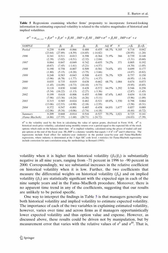
volatility when it is higher than historical volatility (b5/b2) is substantiallynegative in all nine years, ranging from –71 percent in 1996 to –90 percent in2000. Correspondingly, we see substantial increases in the relative coefficienton historical volatility when it is low. Further, the two coefficients thatmeasure the differential weights on historical volatility (b4) and on impliedvolatility (b5) are statistically significant with the expected sign in each of thenine sample years and in the Fama–MacBeth procedure. Moreover, there isno apparent time trend in any of the coefficients, suggesting that our resultsare unlikely to be period specific.

One way to interpret the findings in Table 5 is that managers generally useboth historical volatility and implied volatility to estimate expected volatility.The importance of each of the two variables in explaining estimated volatility,however, varies over time and across firms as if managers opportunisticallylower expected volatility and thus option value and expense. However, asdiscussed above, these results could be driven not by manipulation, but bymeasurement error that varies with the relative values of rI and rH. That is,

Table 5 Regressions examining whether firms’ propensity to incorporate forward-lookinginformation in estimating expected volatility is related to the relative magnitudes of historical andimplied volatilities

εσβσββσβσβασ +×+×++++= IHIHyearindu

D IMPHIIMPHIIMPHI ___ 54321,

SAMPLE 1 2 3 4 5 Adj. R2 N 1+ 4 2+ 5

Pooled 0.230(23.64)

0.498(27.89)

-0.066 (-8.59)

0.488(14.85)

-0.455 (-14.82)

68.3% 9,185 0.718 (20.95)

0.042(1.20)

1996 0.341(2.39)

0.511(3.02)

-0.013 (-0.51)

0.398(2.32)

-0.364 (-2.04)

71.9% 366 0.739(3.31)

0.148(0.60)

1997 0.064(0.67)

0.847(7.45)

-0.049 (-1.61)

0.742(5.21)

-0.655 (-4.57)

74.2% 371 0.805(4.70)

0.192(1.05)

1998 0.190(1.80)

0.758(5.15)

-0.007 (-0.20)

0.509(3.75)

-0.581 (-3.66)

74.6% 451 0.699(4.07)

0.177(0.82)

1999 0.248(3.96)

0.583(6.78)

-0.043 (-1.77)

0.508(5.71)

-0.433 (-4.37)

76.3% 929 0.757(6.95)

0.150(1.14)

2000 0.035(1.45)

0.735(14.09)

-0.019 (-0.73)

0.638(10.10)

-0.662 (-9.73)

68.7% 1,084 0.674 (9.95)

0.073(0.85)

2001 0.118(5.34)

0.830(16.22)

0.040(1.13)

0.428(2.27)

-0.572 (-3.36)

64.5% 1,292 0.546 (2.87)

0.258(1.45)

2002 0.199(7.96)

0.618(13.36)

-0.006 (-0.24)

0.455(4.26)

-0.500 (-5.11)

67.6% 1,465 0.654 (5.96)

0.118(1.09)

2003 0.315(13.06)

0.585(12.53)

-0.024 (-0.90)

0.482(2.18)

-0.521 (-2.55)

69.8% 1,550 0.798 (3.58)

0.064(0.31)

2004 0.372(12.06)

0.547(9.34)

-0.001 (-0.06)

0.485(3.74)

-0.458 (-4.18)

64.8% 1,677 0.857 (6.44)

0.089(0.72)

Summary (Fama-Macbeth)

0.209(4.86)

0.668(17.55)

-0.014 (-1.68)

0.516(20.71)

-0.527 (-24.72)

70.3% 1,021 0.725 (16.03)

0.141(7.39)

σD is the volatility used by the firm in calculating the value of option grants, disclosed in Form 10-K. σH ishistorical stock-price volatility, calculated using monthly returns over a period equal to the expected life of the stock options which ends on the balance sheet date. σI is implied volatility, calculated using the prices of traded call and put options at the end of the fiscal year. HI_IMP is a dummy variable that equals 1 if σI > σH and 0 otherwise. The regressions include fixed effect for industry-year (industry) in the pooled (year-by-year and Fama-MacBeth) regressions, where industry is determined at the 3 digit SIC code level. t-statistics for Fama-Macbeth regressionsinclude correction for auto-correlation using the methodology in Bernard (1995).

b b b b b b bb

E. Bartov et al.

123

even if managers are not opportunistically managing the volatility estimate,they will assign less weight to rI and more weight to rH when rI > rH, andconversely when rI < rH. This alternative explanation is investigated next.

3.3 Opportunistic-behavior explanation vs. measurement errorexplanation

Thus far we have focused on the relation between implied and historicalvolatilities in testing whether firms manage the disclosed volatility parameter.We next use realized future volatility as a proxy for expected volatility andconduct supplementary tests which examine whether measurement error inimplied and/or historical volatility provide an alternative explanation for ourfindings.

It is arguable that the results reported in Table 5, indicating that disclosedvolatility reflects forward-looking information primarily when rI < rH, are dueto the relative magnitudes of measurement error in implied and historicalvolatilities rather than to management of disclosed volatility. More specifi-cally, it is possible that a relatively high volatility value is associated with arelatively high magnitude of measurement error, which makes the volatilitynumber relatively less informative. If so, when rI < rH (rI > rH) firmsappropriately rely less on rH (rI) and more on rI (rH) in deriving rD, as thiswill lead to a more accurate expected volatility estimate.

To assess the validity of this alternative interpretation for our findings,we re-estimate Eq. (2) using two alternative dependent variables: realizedvolatility, rR, and the difference between realized and disclosed volatilities,rD – rR. The results in both Panel A (for the entire sample) and Panel B(subsample with at least 24 months to compute realized volatility) ofTable 6 show that while the measurement error explanation is valid, ourinterpretation that managers shift the weights between historical andimplied volatilities to understate disclosed volatility continues to hold.Specifically, when rR is the dependent variable, b4 is significantly positiveand b5 is significantly negative, which is consistent with the measurementerror explanation. However, a comparison of these coefficients across Eqs.(2) and (3) clearly indicates that the estimates of Eq. (2) are substantiallylarger (in absolute value) than their counterparts in Eq. (3). For example,using the Fama–MacBeth procedure and the entire sample (Panel A), inEq. (2) b4 = 0.516 and b5 = –0.527, while in Eq. (3) b4 = 0.227 andb5 = –0.235. To test the significance of the differences in coefficients, weestimate Eq. (4), where the dependent variable is rD–rR. Consistent withthe opportunistic-behavior explanation, b4 (0.289) is significantly positiveand b5 (–0.292) is significantly negative. Overall, the results in Table 6 leadus to conclude that differential measurement errors in rI and rH can onlypartially explain the results in Table 5, and that the opportunistic-behaviorexplanation is incremental to the measurement error story.


123

Table 6 Regressions examining the importance of measurement error in rH and rI

εσβσββσβσβασ +×+×++++= IHIHindu

D IMPHIIMPHIIMPHI ___ 54321 , (2)

εσβσββσβσβασ +×+×++++= IHIHindu

R IMPHIIMPHIIMPHI ___ ''4

'3

'2

'1

'

5

(3)

IHindu

RD σβσβασσ *2

*1

* ++=− εσβσββ +×+×++ IH IMPHIIMPHIIMPHI ___ *5

*4

*3

(4)

Panel A: Entire sampleDep. Var. 1 2 3 4 5 Adj. R2 N 1+ 4 2+ 5

Pooled RegressionσD 0.230

(23.64) 0.498

(27.89) -0.066 (-8.59)

0.488(14.85)

-0.455 (-14.82)

68.3% 9,185 0.718 (20.95)

0.042(1.2)

σR 0.010(0.93)

0.722(36.33)

0.069(8.14)

0.272(7.43)

-0.241 (-7.04)

53.7% 9,185 0.282 (7.39)

0.481(12.17)

σD - σR 0.220(15.11)

-0.224 (-8.39)

-0.135 (-11.8)

0.216(4.39)

-0.215(-4.67)

21.7% 9,185 0.436 (8.50)

-0.439 (-8.25)

Summary of Annual Regressions (Fama-Macbeth)

σD 0.209(4.86)

0.668(17.55)

-0.014 (-1.68)

0.516(20.71)

-0.527 (-24.72)

70.5% 9,185 0.725 (16.03)

0.141(7.39)

σR 0.272(1.83)

0.556(4.42)

-0.004 (-0.18)

0.227(2.98)

-0.235 (-2.16)

55.2% 9,185 0.499 (4.35)

0.321(12.63)

σD - σR -0.063

(-0.38)0.112(0.77)

-0.01 (-0.6)

0.289(3.18)

-0.292(-2.41)

17.8% 9,185 0.226 (2.12)

-0.180 (-6.85)

Panel B: Subset with at least 24 months to calculate realized volatilityDep. Var. 1 2 3 4 5 Adj. R2 N 1+ 4 2+ 5

Pooled Regression

σD 0.203(19.57)

0.607(31.72)

-0.070 (-8.13)

0.570(16.65)

-0.537 (-16.51)

68.5% 7,330 0.774 (21.62)

0.070(1.86)

σR 0.022(1.76)

0.744(32.6)

0.071(6.94)

0.278(6.80)

-0.249 (-6.41)

51.2% 7,330 0.300(7.02)

0.496(11.01)

σD - σR 0.182

(11.22) -0.137 (-4.59)

-0.14 (-10.54)

0.292(5.49)

-0.289(-5.70)

17.6% 7,330 0.474(8.51)

-0.426 (-7.24)

Summary of Annual Regressions (Fama-Macbeth)

σD 0.227(4.06)

0.682(14.71)

-0.013 (-1.23)

0.577(17.39)

-0.58 (-13.79)

70.8% 7,330 0.804 (23.32)

0.102(4.06)

σR 0.188(3.58)

0.721(16.66)

-0.004 (-0.35)

0.255(3.79)

-0.276(-5.96)

53.7% 7,330 0.443(3.01)

0.445(19.14)

σD - σR 0.039

(0.79)-0.038 (-0.78)

-0.009 (-1.08)

0.322(5.26)

-0.304(-4.05)

15.8% 7,330 0.361(2.86)

-0.343 (-11.68)

σD is the volatility used by the firm in calculating the value of option grants, disclosed in Form 10-K. σH ishistorical stock-price volatility, calculated using monthly returns over a periodequal to the expected option life which ends on the balance sheet date. σI is implied volatility, calculated using the prices of traded call and put options at the end of the fiscal year. σR is realized volatility, calculated using monthly stock returns over a periodequal to the expected options life which starts on the balance sheet date. If the estimation period for realizedvolatility is less than 24 months, daily instead of monthly returns are used (a minimum of 50 daily returns isrequired). HI_IMP is a dummy variable that equals 1 if σI > σH and 0 otherwise. The regressions include fixed effects for industry-year groups for the pooled regressions and industry groups for the year by year regressions,where industry is determined at the 3-digit SIC code level. In Panel B, only those observations are used where 24 months of monthly returns are available for the calculation of realized volatility.

b b b b b b b b b

b b b b b b b b b

E. Bartov et al.

123

3.4 Managerial incentives and ability to understate the option expense

Another alternative explanation for the findings in Table 5 is that impliedvolatility and historical volatility are two alternative estimates for expectedvolatility of equal quality, and following Para. 275 of SFAS No. 123 firmsappropriately pick the lower of the two as their estimate for expected vola-tility. In an effort to assess the validity of this explanation for the prediction ofH3, we examine whether the correlations documented in Table 5 relate to thecosts and benefits of understating the option expense by testing H4.

The benefits from manipulation include lower option expense and lowerperceived top management compensation and wealth. Firms with high levelsof option-based compensation are likely to have strong incentives to under-state expected volatility. However, the downwards manipulation of volatilityis unlikely to be costless as managers and the financial statements they pro-duce are subject to the scrutiny of audit committees, auditors and externalcapital market participants. The costs of manipulating financial disclosuresinclude a negative effect on management’s reputation, a decrease in man-agement’s ability to convey information to the market, an increase in auditcosts and, in extreme cases, potential SEC enforcement actions or shareholderlitigation. These costs are not likely to be identical for all firms. In general,firms facing low levels of monitoring are likely to have relatively low costs andhence high ability to manipulate expected volatility, while firms with highlevels of monitoring are likely to have high costs and low ability to understateexpected volatility.

Recall that in terms of Eq. (2), H4 predicts that b4 (b5) will be increasing(decreasing) in a firm’s incentives/ability to understate the option expense.Conversely, if the estimated coefficients merely reflect the effect of Para. 275,b4 and b5 should be unrelated to incentives/ability. To investigate H4, were-estimate Eq. (2) after partitioning the sample into two groups based oneach variable’s median, where the partitioning variables measure the strengthof managers’ incentives or ability to understate the option expense. If valuesof disclosed volatility reflect incentives/ability, then according to H4, b4[bLow

4

and bHigh5 \bLow

5 , where bHighi is the parameter estimate from the subsample

of firms with high incentives/ability to understate disclosed volatility, and bLowi

is from the low incentives/ability subsample.Table 7 displays the test results of H4 using proxies for incentives (Panel A)

and ability (Panel B) to understate disclosed volatility, as well as the inter-action of the two effects (Panel C). Panel A reports the results using threealternative partitioning variables capturing incentives. The first variable,Option Grants, is the total number of options granted by the firm to allemployees in the year of analysis scaled by shares outstanding. Option grantsgreater (less) than the contemporaneous median for firms in the same 2 digitSIC code are considered large (small). The second partitioning variable,Option Holdings, is the cumulative number of outstanding ESOs (i.e., held byemployees) scaled by shares outstanding. Option holdings greater (less) thanthe contemporaneous median for firms in the same 2 digit SIC code are


123

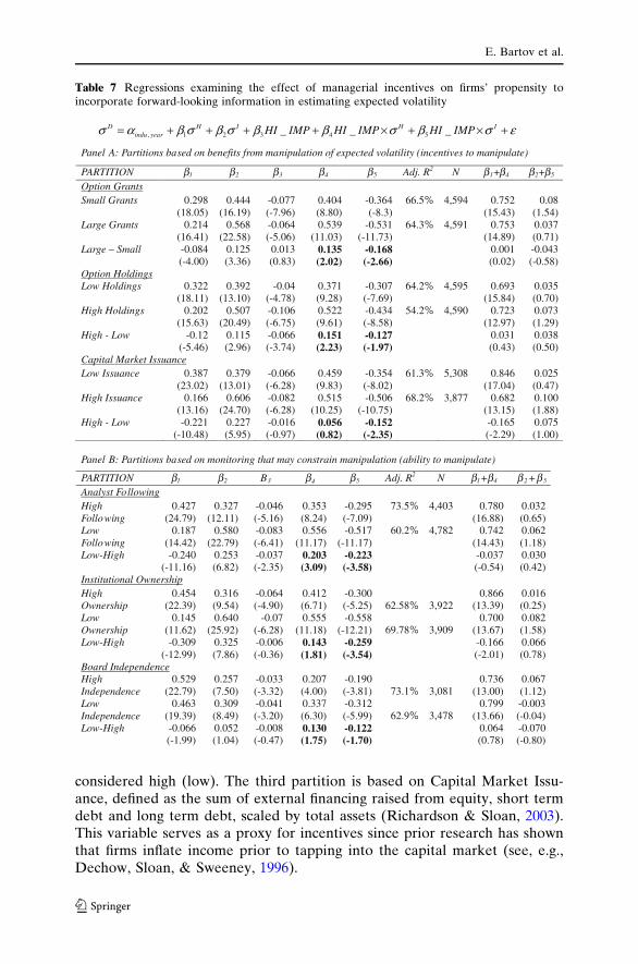
considered high (low). The third partition is based on Capital Market Issu-ance, defined as the sum of external financing raised from equity, short termdebt and long term debt, scaled by total assets (Richardson & Sloan, 2003).This variable serves as a proxy for incentives since prior research has shownthat firms inflate income prior to tapping into the capital market (see, e.g.,Dechow, Sloan, & Sweeney, 1996).

Table 7 Regressions examining the effect of managerial incentives on firms’ propensity toincorporate forward-looking information in estimating expected volatility

εσβσββσβσβασ +×+×++++= IHIHyearindu

D IMPHIIMPHIIMPHI ___ 54321,

Panel A: Partitions based on benefits from manipulation of expected volatility (incentives to manipulate)

PARTITION b1 b2 b3 b4 b5 Adj. R2 N b1+b4 b2+b5

Option GrantsSmall Grants 0.298

(18.05)0.444

(16.19) -0.077 (-7.96)

0.404(8.80)

-0.364 (-8.3)

66.5% 4,594 0.752 (15.43)

0.08(1.54)

Large Grants 0.214(16.41)

0.568(22.58)

-0.064 (-5.06)

0.539(11.03)

-0.531 (-11.73)

64.3% 4,591 0.753 (14.89)

0.037(0.71)

Large – Small -0.084 (-4.00)

0.125(3.36)

0.013(0.83)

0.135(2.02)

-0.168(-2.66)

0.001(0.02)

-0.043 (-0.58)

Option HoldingsLow Holdings 0.322

(18.11)0.392

(13.10) -0.04

(-4.78)0.371(9.28)

-0.307 (-7.69)

64.2% 4,595 0.693 (15.84)

0.035(0.70)

High Holdings 0.202(15.63)

0.507(20.49)

-0.106 (-6.75)

0.522(9.61)

-0.434 (-8.58)

54.2% 4,590 0.723 (12.97)

0.073(1.29)

High - Low -0.12 (-5.46)

0.115(2.96)

-0.066 (-3.74)

0.151(2.23)

-0.127(-1.97)

0.031(0.43)

0.038(0.50)

Capital Market IssuanceLow Issuance 0.387

(23.02)0.379

(13.01) -0.066 (-6.28)

0.459(9.83)

-0.354 (-8.02)

61.3% 5,308 0.846 (17.04)

0.025(0.47)

High Issuance 0.166(13.16)

0.606(24.70)

-0.082 (-6.28)

0.515(10.25)

-0.506 (-10.75)

68.2% 3,877 0.682 (13.15)

0.100(1.88)

High - Low -0.221 (-10.48)

0.227(5.95)

-0.016 (-0.97)

0.056(0.82)

-0.152(-2.35)

-0.165 (-2.29)

0.075(1.00)

Panel B: Partitions based on monitoring that may constrain manipulation (ability to manipulate)

PARTITION b1 b2 B3 b4 b5 Adj. R2 N b1+b4 b 2 +b 5

Analyst FollowingHigh Following

0.427(24.79)

0.327(12.11)

-0.046 (-5.16)

0.353(8.24)

-0.295 (-7.09)

73.5% 4,403 0.780 (16.88)

0.032(0.65)

Low Following

0.187(14.42)

0.580(22.79)

-0.083 (-6.41)

0.556(11.17)

-0.517 (-11.17)

60.2% 4,782 0.742 (14.43)

0.062(1.18)

Low-High -0.240 (-11.16)

0.253(6.82)

-0.037 (-2.35)

0.203(3.09)

-0.223(-3.58)

-0.037 (-0.54)

0.030(0.42)

Institutional OwnershipHigh Ownership

0.454(22.39)

0.316(9.54)

-0.064 (-4.90)

0.412(6.71)

-0.300 (-5.25) 62.58% 3,922

0.866(13.39)

0.016(0.25)

Low Ownership

0.145(11.62)

0.640(25.92)

-0.07 (-6.28)

0.555(11.18)

-0.558 (-12.21) 69.78% 3,909

0.700(13.67)

0.082(1.58)

Low-High -0.309 (-12.99)

0.325(7.86)

-0.006 (-0.36)

0.143(1.81)

-0.259(-3.54)

-0.166 (-2.01)

0.066(0.78)

Board IndependenceHigh Independence

0.529(22.79)

0.257(7.50)

-0.033 (-3.32)

0.207(4.00)

-0.190 (-3.81) 73.1% 3,081

0.736(13.00)

0.067(1.12)

Low Independence

0.463(19.39)

0.309(8.49)

-0.041 (-3.20)

0.337(6.30)

-0.312 (-5.99) 62.9% 3,478

0.799(13.66)

-0.003 (-0.04)

Low-High -0.066 (-1.99)

0.052(1.04)

-0.008 (-0.47)

0.130(1.75)

-0.122(-1.70)

0.064(0.78)

-0.070 (-0.80)

E. Bartov et al.

123

Consistent with the prediction of H4, the results indicate that the ten-dency to understate disclosed volatility by shifting the weights betweenhistorical and implied volatilities is most pronounced when incentives arehigh. Consider, for example, the results for our first proxy–the size of an-nual option grants to all employees. When option grants are relativelysmall, b4 = 0.404 and b5 = –0.364, whereas when they are relatively large,b4 = 0.539 and b5 = –0.531; the differences, b4

Large–b4Small = 0.135 and

b5Large–b5

Small = –0.168, have both the expected signs and are statisticallysignificant at conventional levels.

Panel B reports the results where the partitioning variables are based onthe ability to manipulate disclosed volatility, given the potential costs ofmanipulation. We consider three alternative variables: Analyst Following,Institutional Ownership, and Board Independence. The first two variablesserve as proxies for the extent of monitoring by outsiders that companyexecutives may be subject to. Prior research indicates that firms with a higherlevel of analyst following or institutional ownership are potentially subject to ahigher level of capital market scrutiny. Del Guercio and Hawkins (1999) showthat activist pension funds are more successful in monitoring and promotingchange at target firms. Monitoring by outsiders may also indirectly affect theactivities of insiders such as auditors and audit committees since the latter may

Table 7 continued

Panel C: Partitions based on interaction of expected costs and benefits of manipulation Group COST-BENEFIT PARTITION b1 b2 b3 b 4 b5 Adj. R2 N (1) Low Benefit & High Cost 0.465

(17.04) 0.257(5.99)

-0.096 (-6.33)

0.333(4.35)

-0.136 (-1.89)

64.39% 2,188

(2) Low Benefit-Low Cost orHigh Benefit-High Cost

0.302(15.74)

0.461(13.89)

-0.055 (-4.29)

0.406(6.84)

-0.373 (-6.68)

64.10% 3,557

(3) High Benefit-Low Cost 0.132(8.37)

0.648(19.43)

-0.083 (-4.60)

0.545(7.69)

-0.546 (-8.46)

67.24% 2,086

(3) – (1) -0.333 (-10.57)

0.391(7.21)

0.014(0.58)

0.212(2.03)

-0.410(-4.24)

σD is the volatility used by the firm in calculating the value of option grants, disclosed in Form 10-K. σH is historical stock-price volatility, calculated using monthly returns over a period equal to the expected option life which ends on the balance sheet date. σI is implied volatility, calculated using the prices of traded call and put options at the end of the fiscal year. Panel A considers partitions based on incentives (expected benefits) to manipulate expected volatility. The first partition isthe size of the option grant, defined as the total options granted by a firm to all employees in the year of analysis scaled byshared outstanding. If option grants are greater than (less than or equal to) the contemporaneous median for firms in the same2 digit SIC code it is considered a large (small) grant. The second partition is option holdings, defined as the cumulative number of options outstanding in the firm, scaled by shares outstanding. Option holdings greater than (less than or equal to) the contemporaneous median for firms in the same 2 digit SIC code are considered high (low) holdings. The third partition uses a measure of external financing raised from Richardson and Sloan (2003) as the sum of external financing raised fromequity, short term debt and long term debt (change in #60 – data172 + change in #9 + change in #34 + change in #130),scaled by total assets. Panel B considers partitions based on the strength of monitoring mechanisms (expected costs). The firstpartition is based on analyst following which is measured as the number of analysts issuing one-year ahead EPS forecasts atthe fiscal year end. Firms with analyst following greater than (less than or equal to) the contemporaneous median for firms inthe same 2 digit SIC code are considered to have high (low) following. The second partition is the extent of institutional ownership. Firms with institutional ownership proportion greater than (less than or equal to) the contemporaneous median for firms in the same 2 digit SIC code are considered to have high (low) institutional ownership. The final partition is the extentof board independence, defined as the proportion of board directors that are deemed independent. Firms with proportion ofindependent directors greater than (less than or equal to) the contemporaneous median for firms in the same 2 digit SIC codeare considered to have high (low) independence of boards. In Panel C, we interact one partition based on benefits frommanipulation (option grants) with one partition based on costs of manipulation (institutional ownership.)


123

pay increased attention to sensitive accounting choices when they know thatthose choices are likely to be scrutinized by financial market participants.Indeed, Klein (2002) documents a negative relation between board indepen-dence and abnormal accruals, and also finds that reductions in board inde-pendence are associated with increases in abnormal accruals. Our thirdvariable, which captures the extent of board independence, serves as a moredirect proxy for the level of monitoring that company executives may besubject to by insiders. The ability to manipulate disclosed volatility is likely tobe relatively high with weaker monitoring mechanism, i.e. lower analystfollowing, lower institutional ownership or less independent boards.

Consistent with the predictions of H4, greater weight shifting occurswhen the ability to manipulate is high because of weaker monitoring.Consider, for example, the results for institutional ownership. When theability to manipulate is low because of high institutional ownership,b4 = 0.412 and b5 = –0.300, whereas when the ability is high because of lowinstitutional ownership, b4 = 0.555 and b5 = –0.558; the differences 0.135and –0.259 for b4 and b5, respectively, have both the expected signs and arestatistically significant at conventional levels. Similar results are seen forpartitions based on analyst following or board independence, although thedifferences are only marginally significant for the board independencepartition.

Finally, the results in Panel C are based on the interaction of OptionGrants, a measure of incentives, and Institutional Ownership, a measure of theability to understate disclosed volatility. The sample is partitioned into threegroups: a group of Low Benefit and High Cost, which contains firms withbelow median Option Grants and above median Institutional Ownership, asecond group of High Benefit and Low Cost, which contains firms with abovemedian Option Grants and below median Institutional Ownership, and a thirdgroup which contains all other sample firms. The results from estimatingEq. (2) using the three groups are consistent with those for the individualproxies. Specifically b4 increases monotonically from 0.333 for low incentives/ability group (Group 1) to 0.545 for high incentives/ability group (Group 3),and b5 decreases monotonically from –0.136 for low incentives/ability group to–0.546 for high incentives/ability group. As before, the differences betweenthe coefficients of the two extreme groups, bHigh

4 � bLow4 ¼ 0:212 and

bHigh5 � bLow

5 ¼ �0:410, have the predicted signs and are statistically significantat conventional levels.12

Overall, the picture that emerges from our findings is that firms use bothhistorical volatility and implied volatility in estimating expected volatility, andthat the importance of each of these variables in explaining disclosed volatilityvaries across firms and over time. The crucial determinants underlying the

12 When we use other measures for incentives and ability to manipulate, we consistently find thatb4 (b5) increases (decreases) monotonically from the low incentives/ability group to the highincentives/ability group.

E. Bartov et al.

123

importance of each volatility measure are its relative magnitude and mana-gerial incentives and ability to exploit the discretion inherent in SFAS No. 123to opportunistically understate expected volatility.13

4 Summary and conclusion

To estimate the value of ESOs, firms are required to first derive an esti-mate for expected stock-price volatility. This input parameter has threecharacteristics. First, it is highly discretionary as firms are allowed to useforward-looking information in addition to historical information in settingan estimate. Second, it varies considerably across firms and over time.Third, it has a large effect on the estimated value of ESOs and thus onoption expense. Together, these three characteristics imply that if firms wishto manipulate option expense, the expected volatility parameter would be aprime target. Yet, previous studies examining the parameters used in optionvaluation find mixed results regarding the manipulation of disclosed vola-tility, though they do find that firms manipulate other parameters such asexpected option life. This indicates that the manipulation of volatility, ifindeed it is taking place, may be more sophisticated or more nuanced thanassumed by prior studies, requiring more detailed investigation.

Using a new approach, we address two questions: (1) Do firms follow theguidance in SFAS No. 123 and use both historical and forward-lookinginformation in estimating expected volatility? (2) What are the determinantsunderlying the cross-sectional variation in firms’ tendency to incorporatehistorical volatility and forward-looking information into their expected vol-atility assumption? We find that managers use both historical and forward-looking information in determining expected volatility, consistent with theliteral guidance in SFAS No. 123. We also find, however, that the reliance oneach of the two variables varies inversely with their relative values. One wayto interpret this finding is that managers opportunistically use the discretion inestimating expected volatility afforded by SFAS No. 123 to understate dis-closed volatility. In support of this interpretation, we find that managerialincentives and ability to understate option expense play a key role inexplaining this opportunism.

These results have important ramifications for standard setters decidingabout the extent of discretion to provide managers in estimating parametersfor option valuation. The results indicate that when managers are given the

13 We also conduct three types of sensitivity tests to ensure that our results are robust. First, toverify that our methodology of extrapolating at-the-money implied volatilities does not inducesignificant measurement error, we rerun our tests excluding observations where the nearest strikeprice is more than five percent different from the prevailing stock price. Second, to control forskewness in the distribution of our volatility measures, as well as to account for potential non-linearities in the relationship between our dependent and independent variables, we rerun ouranalyses using: (1) rank regressions, and (2) log transformed variables. Results from all three typesof sensitivity tests (not tabulated for parsimony) are similar to our basic results.


123

alternative of choosing between multiple sources of information, they couldpotentially use that discretion opportunistically.

It is important to note that while our tests are based on data from the SFASNo. 123 period, our results have implications also for its new enacted suc-cessor, SFAS No. 123(R), which specifically advocates considering impliedvolatility in estimating expected volatility in addition to historical volatility.Indeed, companies under the new standard disclose that they follow the newguidance and consider implied volatility, in addition to historical volatility, inestimating expected volatility. For example, UnitedHealth Group disclosed onits Form 10-Q for the first quarter of 2006, ‘‘Expected volatilities are based ona blend of implied volatilities from traded options on our common stock andthe historical volatility of our common stock.’’ Our findings suggest thatfollowing this procedure by itself does not guarantee the integrity of disclosedvolatility. Auditors, investors, and other users of financial statements evalu-ating the appropriateness of a company’s volatility assumption shouldconsider whether the weights given to each factor, historical and impliedvolatilities, are appropriate.

Acknowledgements We would like to thank the editor (Richard Sloan), two anonymous refereesand helpful comments from Menachem Brenner and workshop participants at Columbia Uni-versity, University of Chicago, University of Toronto’s Rotman School of Management, and theSusquehanna International Group LLP 2004 Accounting Research Conference. We appreciateexcellent research assistance from Lucile Faurel, Sharon Katz, Seunghan Nam, and Ron Shalev.Special thanks to David Trainer and Kiran Akkineni of New Constructs for providing disclosedvolatility and option life figures gleaned from Form 10-K’s footnotes.

References

Aboody, D., Barth M., & Kasznik R. (2006). Do firms manage stock-based compensation expensedisclosed under SFAS 123? Review of Accounting Studies, 11(4), 429–461.

Alford, A., & Boatsman J. (1995). Predicting long-term stock return volatility: Implications foraccounting and valuation of equity derivatives. The Accounting Review, 70, 599–618.

Baker, T. A. (1999). Options reporting and the political costs of CEO pay. Journal of AccountingAuditing and Finance, 14, 125–146.

Balsam, S., Mozes, H., & Newman, H. (2003). Managing pro-forma stock-option expense underSFAS No. 123. Accounting Horizons, 17, 31–45.

Bernard, V. (1995). The Feltham–Ohlson framework: Implications for empiricists. ContemporaryAccounting Research, 11(2), 733–747.

Black, F., & Scholes, M. (1973). The pricing of options and corporate liabilities. Journal ofPolitical Economy, 81, 637–654.

Brenner, M., & Subrahmanyam, M. (1994). A simple approach to option valuation and hedging inthe Black–Scholes model. Financial Analysts Journal, 50, 25–28.

Carpenter, J. (1998). The exercise and valuation of executive stock options. Journal of FinancialEconomics, 48, 127–158.

Dechow, P., Sloan, R., & Sweeney, A. P. (1996). Causes and consequences of earnings manipu-lation: An analysis of firms subject to enforcement actions by the SEC. ContemporaryAccounting Research, 13(1), 1–36.

Del Guercio, D., & Hawkins, J. (1999). The motivation and impact of pension fund activism.Journal of Financial Economics, 52, 293–340.

Desai, M. (2002). The corporate profit base, tax sheltering activity, and the changing nature ofemployee compensation. Working paper, Harvard University.

E. Bartov et al.

123

Fama, E., & MacBeth, J. (1973). Risk return and equilibrium: Empirical tests. Journal of PoliticalEconomy, 71, 607–636.

Financial Accounting Standards Board. (1995). Accounting for Stock-based Compensation.Statement of Financial Accounting Standard No. 123.

Financial Accounting Standards Board. (2004). Share-based payment. Statement of FinancialAccounting Standard No. 123(R).

Graham, J. R., Lang, M. H., & Shackelford, D. A. (2004). Employee stock options, corporate taxesand debt policy. Journal of Finance, 59, 1585–1618.

Hemmer, T., Matsunaga, S., & Shevlin, T. (1994). Estimating the ‘‘Fair Value’’ of employee stockoptions with expected early exercise. Accounting Horizons, 17, 23–42.

Hodder, L., Mayew, W., McAnally, M., & Weaver, C. (2006). Employee stock option fair-valueestimates: Do managerial discretion and incentives explain accuracy? ContemporaryAccounting Research, 23(4), 933–975.

Hull, J. (2000). Options, futures, and other derivatives (4th ed.). Upper Saddle River, NJ: PrenticeHall.

Klein, A. (2002). Audit committee, board of director characteristics, and earnings management.Journal of Accounting and Economics, 33, 375–400.

Mayhew, S. (1995). Implied volatility. Financial Analysts Journal, 51, 8–20.Murphy, K. J. (1996). Reporting choice and the 1992 proxy disclosure rules. Journal of Accounting

Auditing and Finance, 11, 497–515.Richardson, S., & Sloan, R. (2003). External financing and future stock returns. Working Paper,

University of Pennsylvania/University of Michigan.Securities and Exchange Commission (SEC). Release No. 33-7032 (November 22, 1993).Standard & Poor’s. Impact of Option Expensing on the S&P 500 Earnings. (November 21, 2005).Watson, J. (1990). Multivariate distributional properties, outliers, and transformation of financial

ratios. The Accounting Review, 65, 682–695.Yermack, D. (1998). Companies’ modest claims about the value of CEO stock options awards.

Review of Quantitative Finance and Accounting, 10, 207–226.


123

managerial discretion and the economic determinants of the ...dn75/doron nissim - managerial...

Documents