management and effects of in-store promotional...

MANUFACTURING & SERVICE OPERATIONS MANAGEMENTArticles in Advance, pp. 1–14

http://pubsonline.informs.org/journal/msom/ ISSN 1523-4614 (print), ISSN 1526-5498 (online)

Management and Effects of In-Store Promotional DisplaysOguz Çetin,a Adam J. Mersereau,a Ali K. Parlaktürka

aKenan-Flagler Business School, University of North Carolina, Chapel Hill, North Carolina 27599-2390Contact: [email protected] (OC); [email protected], https://orcid.org/0000-0002-8349-0388 (AJM);[email protected], https://orcid.org/0000-0002-1495-2614 (AKP)

Received: June 7, 2017Revised: February 19, 2018; August 5, 2018Accepted: August 15, 2018Published Online in Articles in Advance:May 21, 2019

https://doi.org/10.1287/msom.2018.0749

Copyright: © 2019 INFORMS

Abstract. Problemdefinition:Weexamine abrick-and-mortar retailer’s choice ofwhichproductto include in a promotional display (e.g., an “endcap” display). The display provides a visibilityadvantage to both the featured product and its category, but it also has consequences forcustomer traffic and substitution. Academic/practical relevance: Although there has been con-siderable academic interest in the assortment planning problem (which products to offer?)and in the shelf-space allocation problem (how much space to devote to each product?),little attention has been paid to the problem of where to place products in the store. Pro-motional display choice can serve as a powerful demand-shaping lever for retailers. A goodunderstanding of this problem can also facilitate a retailer’s negotiationswithmanufacturers.Methodology:We develop analytical insights using a problem formulation based on a nestedmultinomial logit model of customer choice.Results: When choosing a promotional productfrom a fixed category, the only possible optimal choices for promotional display lie along an“efficient set” drawn in terms of product popularities andmargins. The optimal choice alongthe frontier depends on a quantity we call “aisle attractiveness” that depends on severalcategory-level parameters. The value of the display to a category pivots on whether thedisplay’s role is primarily to expand demand for the category or to shape substitution withinthe category. Managerial implications: Our work provides guidance for how retailers canuse and value promotional displays effectively. We highlight the importance of consideringexternalities of a display decision on store traffic and demand for other products.

Funding: A. J. Mersereau was supported by the Sion A. Boney, Jr. Endowment Fund. A. K. Parlaktürkwas supported by the Benjamin Cone Research Fund.

Supplemental Material: The e-companion is available at https://doi.org/10.1287/msom.2018.0749.

Keywords: retail • assortment planning • promotional displays • choice modeling • nested multinomial logit model

1. IntroductionThere has been considerable research in the opera-tions management literature on the topic of assortmentplanning (i.e., which products to offer?) and to a lesserextent on shelf-space allocation (i.e., how much space todevote to each product?). However, little attention hasbeen paid to the problem of where to place products inthe store. This latter problem is both important andcomplex, as the placement of products in the store isa lever by which the retailer can impact customer trafficpatterns and thereby shape demand across products.Retailers’ merchandising decisions have significant in-fluence on demand because many customer purchasesinvolve some degree of in-store decision (i.e., whether tobuy, or which product to buy). For instance, POPAI(2012) reports that 76% of purchases in supermarketsare either unplanned or planned only up to (but not in-cluding) a specific product choice prior to the shop-ping trip.

In this project we examine an important special caseof the product location problem—namely, the choiceof product to feature in a promotional display. Exam-ples motivating our work include endcap displays in

supermarkets and beverage displays near cashier sta-tions in convenience stores. Although there is work inthe marketing literature seeking to understand cus-tomer behavior in stores and to measure the impact ofproduct placement decisions and price and advertisingpromotions, we are not aware of existing research pro-viding prescriptive insights for the complex decision ofwhich product to feature in a promotional display. Ourwork seeks to fill this gap.A display provides a visibility advantage to the

featured product over products stocked only in theregular shelf space. We can decompose the impact ondemand for products in the category into two effects:(1) the display expands the overall category demand bycapturing the attention of some customers who wouldnot otherwise have purchased from the category (the“demand-expansion effect”), and (2) it may inducesome customers to substitute the promoted productfor their original preference (the “substitution effect”).We model both effects. We note that both effects canbe present in themore traditional assortment planningproblem, but the promotional display decision givesthe retailer an additional degree of freedom. That is,

1

http://pubsonline.informs.org/journal/msom/

mailto:[email protected]


https://orcid.org/0000-0002-8349-0388

https://orcid.org/0000-0002-8349-0388


https://orcid.org/0000-0002-1495-2614

https://orcid.org/0000-0002-1495-2614



the promotional display decision allows the managerto modulate the category’s visibility and to shape sub-stitution patterns even given a fixed assortment. Fur-thermore, it can be changed more easily and thereforemade more dynamically than the assortment decision.

We assume that the set of products in the categoryassortment is exogenously given, as are the profit marginsand mean utility (or popularity) of each product. Thispermits us to focus specifically on the effect of the display.All products in a category are colocated in a native “aisle”location, and at most one is selected also to be featuredin the promotional display. We assume ample stock ofall products.

We employ the nested multinomial logit (NMNL)framework to model customer choice within a cate-gory, which we interpret as a two-stage choice process.The customer first encounters the promotional display(if present) and chooses whether to purchase the fea-tured product, visit the category’s aisle location, or leavewithout purchasing from the category. A customer whovisits the aisle may choose among the full assortment ofproducts or may choose not to purchase. We assumethat a customer who visits the aisle incurs a constantdisutility representing the transit cost. The retailer col-lects the profit margin associated with any purchasedproduct plus a bonus margin from any customer whovisits the aisle. This bonus margin captures the expectedmargin of any impulse buys or complementary productsthe customer encounters on visiting the aisle.

Following a review of relevant literature (Section 2)and the introduction of our model (Section 3), we presentour analysis in three parts. In Section 4, we examine thechoice of product to promote from a given category.We show that the retailer can immediately eliminatesomeproducts from consideration based only onmarginand popularity characteristics. The remaining productsform an “efficient set” within which higher popularityimplies lower margin and vice versa. Intuitively, fea-turing a popular product in the display minimizes thechances of customers leaving empty-handed, whereaskeeping popular, low-margin products in the aislemaximizes both margins at the display and additionalimpulse spending in the aisle. We prove that the lat-ter strategy is optimal when an aisle visit is inherentlyattractive to customers, which is the case when the aisleassortment is relatively large, when customers are he-terogeneous in their preferences, and when the tran-sit cost is low. An example implication is that popularproducts are good choices for endcap displays in largestore footprints where customers incur high transit coststo visit an aisle. Moreover, high-margin products, thoughat a potential popularity disadvantage, work better ina display when the category demand is spread outacross multiple products in a large assortment.

In Section 5 we analyze the value of the promotionaldisplay across categories, assuming that the optimal product

from each category would be promoted as described inSection 4. A key factor is the strength of the demand-expansion effect for a category. We assume that thedegree to which the promotional display can increasepotential demand differs across categories, as some cate-gories have an impulsive nature whereas others are moreutilitarian. Clearly, the value of the promotional display isgreatest when the demand-expansion effect is strongest.Moreover, when the demand-expansion effect is strong,the value of thedisplay increases in the attractiveness of theaisle (determined by the assortment size, customer het-erogeneity, and transit cost); the opposite is true when thedemand-expansion effect is weak. This implies that thedisplay should be reserved for two classes of product cate-gories: those with high demand-expansion upside andan attractive aisle option, and thosewith stable category-level demand but a less appealing aisle option.The analyses described so far assume that all products

from a category are equally effective at generatingawareness for the category when placed in the pro-motional display—that is, the demand-expansion effectis category specific but not product specific. (We notethat even under this assumption, products will differ intheir ability to generate sales from the display becauseof the substitution effect.) We believe this assumptionis natural, though we are not aware of empirical evi-dence establishing whether demand-expansion effectsare product specific. For completeness, in Section 6 weconsider product-specific demand-expansion effects andrevisit our results on the choice of product to promotefrom a category.We require additional assumptions thatwe specify for our efficient set result to hold. We alsodemonstrate that the core directional forces identifiedin Section 4 remain in effect, but the forces operate inthe directions of new product indices that depend onproducts’ demand-expansion abilities.Throughout the paper, we take the retailer’s perspec-

tive, and we assume that the retailer behaves myo-pically, focusing on optimizing profits in the currentperiod. However, we recognize that the retailer does notmanage promotional displays in a vacuum. In practicethere are negotiations over promotional displays be-tween retailers and manufacturers, often resulting inmanufacturers offering incentives to retailers to featurecertain products. Product popularities may also dependon past promotions due to saturation and stockpilingeffects. Although we do not model these coordinationactivities and dynamics directly, we believe that un-derstanding the retailer’s incentives with respect toproduct margins (which can be dynamically influencedby manufacturer discounts) and product popularities(which can be influenced by other types of promo-tional activities) is an important building block for un-derstanding these coordination activities and dynamics.Proofs of all analytical results are presented in the

e-companion.

Çetin, Mersereau, and Parlaktürk: Management of In-Store Promotional Displays2 Manufacturing & Service Operations Management, Articles in Advance, pp. 1–14, © 2019 INFORMS

2. Related LiteratureOur study is related to a large literature on assortmentplanning, where the typical goal is to specify the set ofproducts carried in a store (or in a sales channel) tomaximize sales or gross margin under constraints onshelf space or on purchasing budget. A driving factor inthis literature is customers’ potential to substitute anavailable product when their original preference is notoffered in the assortment, called assortment-based sub-stitution (Kok et al. 2008). Substitution in our paper arisesfrom the visibility advantage of a product featured ina promotional display.

We employ the nested multinomial logit (NMNL)model to capture the aforementioned substitution ef-fect. The NMNL model is commonly used in empiricalchoice models as a more flexible extension of theclassical multinomial logit model (Train 2009). It is alsocommonly used to model two-stage choice scenarios(Manrai and Andrews 1998). An early use of it in theliterature on demand for consumer packaged goods isGuadagni and Little (1998), who use it to captureconsumers’ intertemporal preferences for buying nowversus later. Kok and Xu (2011) use it to capture cus-tomers’ choices among brands then product types, oramong product types then brands. Davis et al. (2014)and Gallego and Topaloglu (2014) consider nests asdifferent sales channels or different stores. Aouad andSegev (2015) and Feldman and Topaloglu (2015) modelnested consideration sets formed by online searchrankings or cutoffs on attributes like quality or price.Our two-stage choice scenario has a spatial interpre-tation as discussed in Section 3. The nests in our settingrepresent different locations (display or aisle) in the store.Davis et al. (2013) also consider location-specific prefer-ence weights in a multinomial logit model. They assumeexogenously given preference weights, whereas we ex-plicitly model the factors that determine the relative at-tractiveness of a product in different locations.

A natural constraint in assortment planning is on shelfspace. Early research on shelf space allocation de-velops algorithms for large-scale problems (Corstjens andDoyle 1981, Bultez and Naert 1988). More recent stud-ies (Bai et al. 2013, Geismar et al. 2015) incorporate thevertical alignment of products on the shelf that im-pacts product visibility. Our research does not considershelf space or vertical alignment, though we considerthe visibility difference between the regular shelf spaceand the promotional display, which arguably provides amore profound visibility advantage to the focal product.Wilkinson et al. (1982) report that the percentage increasein unit sales is between 16%and 39%with expanded shelfspace, but between 77% and 243% with secondary dis-plays for the four products they examine.

Customers’ impulse spending figures prominentlyin our problem. Conventional wisdom suggests thatexposure to in-store stimuli leads to impulse spending

(Inman andWiner 1998, Hui et al. 2013). In our case, thepromotional display triggers impulse spending on thefeatured product, but it also diverts some customersfrom the aisle due to substitution. Our model penalizesthe loss in aisle traffic by explicitly capturing the po-tential impulse spending of customers in the aisle.A stream of papers in the marketing literature em-

pirically studies how the impact of a promotional dis-play depends on factors such as the demand dispersionwithin the category (Chevalier 1975), display’s distanceto the product’s own aisle location (Nordfalt and Lange2013, Phillips et al. 2015), and to a complementary cat-egory’s aisle location (Bezawada et al. 2009). Moreover,Dhar et al. (2001) study how demand expansion ofpromotional displays can vary across categories. Zhang(2006) models how customers form consideration setsvia displays. We incorporate all of these factors in ourmodel. These papers do not consider the optimal productchoice for promotional display, and they tend to focuson the impact of external factors (e.g., day of the week,whether the display is assisted by a personnel or afeature ad) on the effectiveness of promotional display.In contrast, we characterize the optimal product andcategory choice based on their characteristics.VanHeerde andNeslin (2017) provide a recent review

of the marketing literature that empirically studies theeffect of price promotions. These papers focus on under-standing the sales lift of the promoted product resultingfrom demand expansion (primary) and the substitution(secondary) effects by studying household-level (Gupta1988, Chintagunta 1993, Bell et al. 1999, Pauwels et al.2002, van Heerde et al. 2003) and store-level (van Heerdeet al. 2004, Nair et al. 2005) data. Our model considersboth primary and secondary effects of display promotions.However, different from these studies, we take theretailer’s perspective and consider the effects of thesepromotions on the retailer’s profit and hence considerthe impact of these promotions on all other products aswell. In addition, we take into account the impact ofa promotion on customer traffic within the store. Thevalue of driving customers to a particular aisle is a corecomponent of our model.Cross-category effects of price promotions (Ailawadi

et al. 2006, Leeflang et al. 2008, Leeflang and Parreño-Selva 2012) and displays (Bezawada et al. 2009) are wellestablished in the literature. Although we do not ex-plicitly model a cross-category effect of promotions, wecapture complementarity between categories by ac-counting for average impulse spending on other cat-egories when a customer visits the aisle.

3. Model SetupWe consider a category consisting of n ≥ 2 products,andwe indicate this set of products by S � {1, .., n}. Eachproduct is characterized by its associatedmeanutility Yj

and its profit margin mj. To simplify our exposition,

Çetin, Mersereau, and Parlaktürk: Management of In-Store Promotional DisplaysManufacturing & Service Operations Management, Articles in Advance, pp. 1–14, © 2019 INFORMS 3

we assume that no pairs of products have the samemean utility and profit margin. The retailer has theoption of promoting one of the products by featuring itin an in-store promotional display (“display” hereafter)in addition to its regular shelf space in the aisle. We use“aisle” to refer the location in the store permanentlyallocated to the category. Each product in the categoryhas its own shelf space in the aisle, and we do notmodel any differences in the shelf space allocated toproducts. We assume that prices are exogenous andare reflected in the margin and popularity parameters.

We employ theNMNL choice framework for twomainreasons. First, it is a random utility model of customerchoice that is consistent with utility-maximizing be-havior, that extends the classical MNL model, and thatyields closed-form choice probabilities (McFadden 1978).Second, the choice probabilities in the NMNL modelcan be decomposed into two stages whereby individualsfirst choose a nest and then choose an alternativewithinthe chosen nest to maximize their utility (Train 2009).This fits nicely with a natural interpretation of cus-tomer choice in our problem as a two-stage decisionprocess as shown in Figure 1. (Some of the notations inFigure 1 will be defined later in this section, and areincluded in the figure for completeness.)

In the NMNL model, the utility Uj associated withalternative j in nest k has the following form:

Uj � Yj +Wk + εj, (1)

whereYj andWk are alternative-specific andnest-specificdeterministic components of the utility, respectively.The random component, εj, captures the idiosyncraticutility of a customer and enables heterogeneity in cus-tomers’ choices. The εj’s are assumed to follow a gen-eralized extreme value distribution with the joint c.d.f.

Φ(ε) � exp −∑Kk�1

∑j∈Bk

e−εj/λk

( )λk

{ }, (2)

where Bk is the set of alternatives in nest k. The dif-ference between the MNL and the NMNL models isthat the latter allows correlation between (εi, εj) pairscorresponding to alternatives i and j within the samenest, and the parameter λk ∈ 0, 1( ] of the joint c.d.f.Φ(ε)

specifies this correlation structure for nest k. In par-ticular, (1 − λk) is a measure of the correlation between(εi, εj) corresponding to any two alternatives (i, j) withinnest k (Train 2009).In our choice scenario, each customer makes a de-

cision among three options in stage 1: to purchase fromthe display, to visit the aisle to see all available prod-ucts, or to neither purchase nor visit the aisle. Theseoptions represent the nests in our NMNL model, andwe index these nests by “D” (display), “A” (aisle), and“0” (no-purchase), respectively. We assume that cus-tomers incur a “transit cost” if they visit the aisle, whichwemodel as a nest-specific disutility, c, associated withthe nest corresponding to the aisle; that is, WA � −c.Note that the nests 0 andD include only one alternativeeach, implying that λ0 and λD are irrelevant and onlyλA has an impact on the choice probabilities. Hence, wedrop the subscript in λA and consider λ as the pa-rameter determining the level of correlation among theutilities associated with the alternatives in the aisle.There are n + 1 alternatives in nest A, correspondingto n product variants and a no-purchase alternative.Therefore, our model assumes that the product beingfeatured in thedisplay is also available in the aisle (matchingthe grocery and convenience store cases that motivatedour study), and it allows for customers not to purchaseeven after visiting the aisle (which is consistent withcustomers learning their value realizations for individualaisle products on reaching the aisle). We note that certainpromotional display settings in practice, such as pro-minent tables in apparel stores, differ from groceryand convenience store settings in that the same productmay not be simultaneously available in two locations.We note that an assumption of the NMNL model is

that εj’s corresponding to alternatives in different nestsare independent. This may not strictly be the case in oursetup because the featured product appears in both thenestsD andA, andwewould expect a correlation amongthe utilities for the same product in two locations. Wenevertheless use the standard NMNL assumption asan approximation with the benefit of yielding closed-form choice probabilities, noting that this approxi-mation may underestimate the demand generated bythe display (see Guadagni and Little 1998 for a similarassumption).

Figure 1. (Color online) Customer Choice Modeled as a Two-Stage Decision Process


We measured the impact of this independence as-sumption in a numerical simulation in which customers’utilities for the featured products in nests D and A arecorrelated. Our simulation model relies on a decompo-sition of the random error term εj into nest-specific (νk)and product-specific (ξj) components such that εj � νk +λξj [see Besanko et al. (1998) and Berry (1994) forthe same decomposition, and Cardell (1997) for thedistributional properties of νk and ξj]. We capture theaforementioned correlation by fixing a customer’s re-alization of the random term ξ(·) corresponding to thefeatured product in the two locations (display andaisle). We similarly model correlation between the no-purchase option in the display and aisle. To generaterandom utilities requires sampling from complicatedprobability distributions. We present some of the tech-nical details and results of the simulation in Appendix B.In short, we find that assuming independence degradesoptimal profits by just 0.5% on average in our simulationsand that the directional insights of Section 4 continueto hold for most instances when we model thesecorrelations.

Throughout the paper, superscripts denote the productfeatured in the promotional display. When product i ∈S is in the promotional display, the associated first-stage probabilities, denoted by Pi

0, PiD, and Pi

A are asfollows:

Pi0 � P{no purchase from display and no aisle visit}� eY0

eY0 + eYi + e−c+λ·I,

(3)PiD � P{purchase from the display}� eYi

eY0 + eYi + e−c+λ·I,

(4)

PiA � P{visit the aisle} � e−c+λ·I

eY0 + eYi + e−c+λ·I, (5)

where Y0 is the utility associated with the no-purchasealternative and I � ln

(∑j∈S∪{0} eYj/λ

). The quantity I is

often called the “inclusive value” of a nest in NMNLmodels. It links the first and second stages of thedecision-making process by conveying informationabout the expected value of the aisle as viewed from thefirst stage. The expected maximum utility obtainedfrom nest k isEε

[maxj∈Bk Yj + εj

{ }] � λkIk + γ, whereγ ≈0.5772 is Euler’s constant (McFadden 1978). Therefore,the expected utility of choosing the aisle option in thefirst stage is the sum of the expected utility obtainedby choosing the best alternative in the aisle (λ · I) andthe transit cost (−c). Note that parameter γ is irrelevantin the first-stage probabilities because it is commonacross all nests.

We denote the second-stage probability of product j—i.e., the conditional probability of choosing productj given that the customer visits the aisle—by pj|A. Wehave pj|A � eYj/λ/

∑q∈S∪{0}eYq/λ for j ∈ S∪{0}. When pro-

duct i is in the display, the unconditional probability ofchoosing product j in the aisle is Pi

A ·pj|A for j∈S∪{0}.Notice that the probability of choosing product j in theaisle is proportional to eYj/λ. Since λ is the same for allproducts in the aisle, we refer to eYj as the “popularity” ofproduct j.We can interpret the parameter λ as a measure of

“customer heterogeneity.” In Figure 2, we illustrate thesecond-stage choice probabilities in the two extremes,when λ � 10−3 and λ � 1, for a set of five fictitiousalternatives with fixedmean utilities Y. When λ � 10−3,the random components of the associated utilities arealmost fully correlated, so the alternative associatedwith the highest mean utility (alternative 1) is chosenwith probability close to 1. On the other hand, therandom components of the associated utilities are in-dependent when λ � 1, so the choice probabilitiesspread out across alternatives in this case.To express the retailer’s expected profit per customer,

we must consider the two sources of the retailer’s profit:(1) the customer’s potential purchase of one of theproducts in the focal category, and (2) the impulsespending in case the customer visits the aisle. The im-pulse spending in the aisle contributes to a key aspect ofourmodel, which is the value of driving customers to theaisle. Indeed, customer aisle visits can result in additionalcomplementary purchases; therefore, we assume that theretailer expects to earn r per customer as a result of thisunplanned spending. In practice, retailers try to attractcustomers to the aisles by strategically deciding productlocations (Rupp 2015). Moreover, Hui et al. (2013) pointout that “encouraging customers to travel more of thestore may increase unplanned spending by exposingthem to more product stimuli.” Lastly, POPAI (2012)reports that the percent of basket purchases on impulseincreases in the number of aisles visited by a customer.Let πi denote the expected profit per customer when

the retailer chooses product i to promote in the display.For brevity, we define m(Y,m, λ) � ∑

j∈S pj|A ·mj, which

Figure 2. (Color online) Second-Stage Choice Probabilities(pi|A) when λ � 10−3 and λ � 1 for Y � 〈0.5, 0.4, 0.3, 0.2, 0.1〉


is an average of the margins of all products in thecategory weighted by the second-stage probabilities.We can express πi as

πi � PiD ·mi + Pi

A · m(Y,m, λ) + r( ), i ∈ S. (6)

The first term of Equation (6) arises because ifproduct i ∈ S is featured on the display, an averagecustomer purchases the featured product from thedisplay with probability Pi

D, in which case the retailercollects the profit margin mi of the focal product. Al-ternatively, the average customer visits the aisle withprobability Pi

A, where she is expected to spend an amountof m(Y,m, λ) + r( ). Finally, the average customer choosesnot to purchase from the category with probability Pi

0,in which case the retailer’s profit is 0.

We discussed in the introduction that a promotionaldisplay has two primary impacts on demand: it expandsthe potential overall category demand by evoking thecategory in customers’ minds (the demand-expansioneffect), and it boosts demand for the focal product at theexpense of competitor products and of the no-purchaseoption (the substitution effect). The model developed sofar represents our core model of baseline demand, ac-counting for the substitution effect only. We will laterextend it to reflect the demand-expansion effect. Underthe assumption that all products from a category areuniformly good at generating demand expansion forthe category, the model presented here is sufficient forour study of the choice of product from a category(Section 4). Demand-expansion effects will become rel-evantwhenwe consider the value of promotional displaysacross categories (Section 5) and product-specific demand-expansion effects (Section 6).

Throughout Sections 4 and 5 we will make the fol-lowing assumption that the expected impulse spendingin the aisle (r) is not too high.

Assumption 1. maxi∈S{mi}>P0A · m(Y,m,λ)+r( ), where

P0A� e−c+λ·I

eY0+e−c+λ·I .

This assumption ensures that promoting some prod-uct in S is more profitable than promoting a hypotheticalproduct j with preference weight eYj � 0 (equivalently,Yj � −∞.) We will motivate and present a modificationto this assumption in Section 6.

4. Product ChoiceAs discussed previously, in this section we examine theretailer’s choice of which product from a given categoryto feature in a promotional display. We leave the valu-ation of the display across categories to Section 5.

This section is organized as follows. In Section 4.1 weeliminate some of the products from considerationbased solely on their product characteristics (specifi-cally, margin and popularity) irrespective of the cate-gory parameters r, c, and λ, thereby reducing the full

category of products to an “efficient subset” of productsthat are candidates for the promotional display. InSection 4.2 we consider how the retailer’s optimal choiceof product to promotewithin the efficient subset changeswith respect to the category parameters.

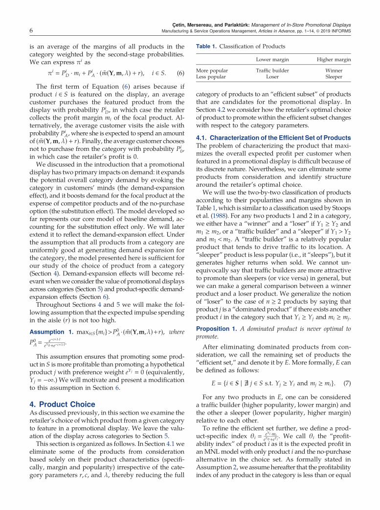
4.1. Characterization of the Efficient Set of ProductsThe problem of characterizing the product that maxi-mizes the overall expected profit per customer whenfeatured in a promotional display is difficult because ofits discrete nature. Nevertheless, we can eliminate someproducts from consideration and identify structurearound the retailer’s optimal choice.We will use the two-by-two classification of products

according to their popularities and margins shown inTable 1,which is similar to a classification used by Stoopset al. (1988). For any two products 1 and 2 in a category,we either have a “winner” and a “loser” if Y1 ≥ Y2 andm1 ≥ m2, or a “traffic builder” and a “sleeper” if Y1 >Y2and m1 <m2. A “traffic builder” is a relatively popularproduct that tends to drive traffic to its location. A“sleeper” product is less popular (i.e., it “sleeps”), but itgenerates higher returns when sold. We cannot un-equivocally say that traffic builders are more attractiveto promote than sleepers (or vice versa) in general, butwe can make a general comparison between a winnerproduct and a loser product. We generalize the notionof “loser” to the case of n ≥ 2 products by saying thatproduct j is a “dominated product” if there exists anotherproduct i in the category such that Yi ≥ Yj and mi ≥ mj.

Proposition 1. A dominated product is never optimal topromote.

After eliminating dominated products from con-sideration, we call the remaining set of products the“efficient set,” and denote it by E. More formally, E canbe defined as follows:

E � {i ∈ S | e j ∈ S s.t. Yj ≥ Yi and mj ≥ mi}. (7)

For any two products in E, one can be considereda traffic builder (higher popularity, lower margin) andthe other a sleeper (lower popularity, higher margin)relative to each other.To refine the efficient set further, we define a prod-

uct-specific index θi � eYi ·mieY0+eYi . We call θi the “profit-

ability index” of product i as it is the expected profit inan MNLmodel with only product i and the no-purchasealternative in the choice set. As formally stated inAssumption 2, we assumehereafter that the profitabilityindex of any product in the category is less than or equal

Table 1. Classification of Products

Lower margin Higher margin

More popular Traffic builder WinnerLess popular Loser Sleeper


to the expected profit obtained from the aisle, condi-tional on the customer visiting the aisle.

Assumption 2. Product characteristics Y and m are suchthat θi ≤ m(Y,m, λ) + r( ) ∀i ∈ S.

When this assumption is violated the problem be-comes trivial and the retailer would be better off of-fering product i alone in the display and removing all ofthe other products from the aisle. By using the prof-itability index, we can further refine the efficient set asstated in Proposition 2.

Proposition 2. Consider two products, i and j, such thatYi <Yj. It is never optimal to promote product j if θi ≥ θj.

Proposition 2 says that any promoted productshould have a higher profitability index than all of theother less popular products in the efficient set. Let E′denote the set of products remaining in the efficient setafter refining according to Proposition 2, ormore formally,

E′ � {i ∈ E | e j ∈ E s.t.Yi >Yj andθj ≥ θi}. (8)

Hereafter, we order products in E′ such thatY1 > ..>Y|E′ |and m1 < ..<m|E′ | w.l.o.g. Therefore, products with lowindices can be considered traffic builders relative toproductswith higher indices (sleepers).Note thatwe alsohave θ1 > ..>θ|E′ | by Proposition 2.

To highlight the importance of the retailer’s productchoice, we compared in a numerical study the optimalexpected profit to those of three natural heuristic policies—in particular, policies choosing the most popular product(Y-Policy), the highest margin product (m-Policy), andthe product with the highest profitability index (θ-Policy).In Table 2,we report the average andmaximumoptimalitygaps over 100 synthetically generated product categoryinstances, each of which includes 15 products. Eachproduct is characterized by its mean utility Y and theprofit margin m that are randomly chosen from twouniform distributions with a certain correlation. Weconsidered four different combinations of the impulsespending parameter r and the transit cost parameter c.(The details of the parameter settings are presented inAppendix A.)

Note that the Y-Policy performs remarkably worsethan the other two policies on average, because it oftenchooses a product from outside the set E′. The θ-Policyperforms the best of the three heuristics on average.Thismakes sense in light of Proposition 2, which suggests

that products with higher profitability index θitend to be favored within the set E′. Although per-forming well on average, the m-Policy and θ-Policymay still lead to losses as large as 18% and 7%, re-spectively. The m-Policy’s worst average performance(8%) is when r is low and c is high, whereas the θ-Policy’s best average performance (0.4%) is achievedin that scenario. In addition, θ-Policy’s worst aver-age performance (1.21%) is when r is high and c is low,whereas them-Policy’s best average performance (0.58%)is achieved in that scenario. This reinforces the im-portance of understanding the optimal policy as afunction of the problem parameters.

4.2. Sensitivity Analysis on Retailer’sOptimal Decision

The refined efficient set E′ is defined only in terms ofproduct popularities and margins, and is indepen-dent of values of the category parameters r, c, and λ.However, the optimal choice of product from E′ de-pends on the category parameters, and here we seek tounderstand these dependencies.We use i∗(·) � argmaxi∈S{πi(·)} to refer to the re-

tailer’s optimal choice of product to promote. The or-dering of products in E′ implies that promoting a lowerindexed product (traffic builder) yields higher expectedprofit from the display (Pi

D ·mi), but lower expectedprofit from the aisle (Pi

A · (m + r)) compared witha higher indexed product (sleeper). Hence, the retailer’sdecision among products in E′ trades off the display andthe aisle profits.Intuitively, this decision depends on two factors: the

aisle’s attractiveness for customers, and its profitabilityfor the retailer. As mentioned in Section 3, the quantityλ · I(Y, λ) shows a customer’s expected utility obtainedby choosing her best alternative in the aisle. Hence, wecall the quantity e−c+λ·I(Y,λ) the “aisle’s attractiveness.”Likewise, we call the quantity m + r( ) the “aisle profit.”4.2.1. Parameters r and c. The transit cost c incurred bycustomers to reach a category’s aisle space varies withseveral store- and category-specific factors. First, largestore footprints are associated with higher search costsbecause the store size has a direct impact on customers’walking distance within the store to find the productsthey are looking for (Baumol and Ide 1956, Trivedi et al.2016). Second, Larson et al. (2005) provide empirical

Table 2. Percentage Optimality Gaps Corresponding to Three Heuristic Policies

Y-Policy m-Policy θ-Policy

r c Average Maximum Average Maximum Average Maximum

Low Low 7.73 12.16 2.42 5.99 0.50 3.80Low High 13.29 22.02 8.06 17.71 0.40 4.05High Low 8.07 11.39 0.58 2.29 1.21 5.90High High 13.36 20.58 4.34 10.57 0.98 6.99


evidence that grocery store customers tend to walkalong the perimeter of the store, visiting a particular aisleonly if a product they are looking for appears in thataisle. Hence, the proximity of the product category to theperimeter of the store is a determinant of how muchcustomers need to deviate from their base trajectorywithin the store. Third, c may also vary with customers’expectation for convenience—for example, in a “con-venience” store setting c will reflect customers’ highdisutility to spending extra time in the store.

Similarly, the impulse parameter r is a category-specific parameter that depends on the complemen-tarity of the categorywith other categories placed in thesame aisle. Practitioners consider cross-category saleswhen deciding floor space allocation, and empirical re-searchers often consider specific pairs of colocated cat-egories to tease out cross-category effects—for example,cola and potato chip categories (Bezawada et al. 2009),detergent and fabric softener categories (Manchandaet al. 1999). Proposition 3 shows the ceteris paribusimpact of the parameters r and c on i∗(·).Proposition 3. The following statements hold:

1. i∗(r) is nondecreasing in the expected impulse spending r.2. i∗(c) is nonincreasing in the transit cost c.

The proposition states that as expected impulsespending r increases, the optimal product to promotemoves toward sleeper products. Increasing r increasesthe aisle profitability, driving the retailer toward fea-turing sleeper products in the display to keep aisle traffichigh. On the other hand,when transit cost c increases, theaisle becomes unattractive to customers, and the re-tailer seeks to emphasize display profits, captured by theimmediate profitability θi. Recall that by Proposition 2,immediate profitability increases with the popularity ofthe featured product. These intuitions—that high aisleprofits drive the retailer to keep traffic builders in theaisle, and that unattractive aisles tend to favor featuringprofit-driving products—underlie all of the results onproduct choice to follow.

4.2.2. Assortment Size. Next, we consider the effect ofassortment size on the retailer’s promotion choice. As-sortment sizes vary across categories for a given retailer,and retailers vary in their assortment sizes for a givencategory. A larger assortment implies a more attrac-tive aisle for customers, consistent with the conventionalwisdom that customers value variety. In our model,a larger assortment translates to a higher inclusive valueI(Y, λ) and hence a more attractive aisle. Specifically, itholds that I(YS, λ)< I(YS+ , λ) for two assortments S andS+ such that S ⊂ S+.

Proposition 4. Consider two assortments S and S+ suchthat S ⊂ S+ and m(YS,mS) � m(YS+ ,mS+). Then, we haveargmaxi∈S{πi(S)} ≤ argmaxi∈S{πi(S+)}.

We restrict the choice to the set S and assume equalaverage margins m to focus our insight on the impactof assortment breadth.A recent examination of Target.com reveals that

a specific Target store carries 14 brands of liquid laundrydetergent and 102 brands of hair shampoo, implying thatcategories can vary significantly in assortment size.Assuming all else fixed, Proposition 4 implies that arelatively higher-margin and lower-popularity product(i.e., a sleeper) will tend to be preferred for the shampoocategory because of its large assortment, whereas theopposite is true for laundry detergents.

4.2.3. Customer Heterogeneity Parameter λ. The lastfactor we consider to have an impact on the aisle’sattractiveness is the customer heterogeneity parameterλ. As mentioned in Section 3, λ specifies the correlationamong the random components of the utilities associatedwith the alternatives in the aisle. In particular, as λ in-creases in the interval (0, 1], the random utility compo-nents become less dependent. This has implications onboth the first- and second-stage choice probabilities.Since m(Y,m, λ) and I(Y, λ) are functions of λ, both theaisle profit for the retailer and the aisle’s attractivenessfor the customers depend on the customer heterogeneity.

Lemma 1. The aisle’s attractiveness, e−c+λ·I(Y,λ), is in-creasing in λ in the interval 0, 1( ].Lemma 1 implies that the aisle is more attractive for

customers when their preferences are more heteroge-neous. In other words, the same assortment in the aisleis appreciated more and attracts more customers whencustomers aremore heterogeneous in their choices. GivenLemma 1, we can state the following result on the impactof λ on the retailer’s optimal promotional display choice.

Proposition 5. Assume that the average profit marginm(Y,m, λ) is nondecreasing in λ. Then, i∗(λ) is non-decreasing in λ.

The intuition here is similar to that of Proposition 3,part 2: promoting a sleeper product makes sense whenthe aisle is attractive. By Lemma 1, the aisle is mostattractive for large λ. The assumption on the averageprofit margin holds if products’ profit margins andpopularities generally have an inverse relationshipwithin a category. This is likely to be the case in practicebecause higher profit margin is needed to compensatefor lower sales volume, and Vilcassim and Chintagunta(1995) show that optimal retailer profit margins areconsistent with this intuition.Considering its impact on the second-stage choice

probabilities as shown in Figure 2, the customer het-erogeneity parameter λ can be considered a proxy formarket structure. That is, a small λ leads to a concen-trated market in which most customers choose the sameproduct, whereas larger λ leads to a diversified marked


http://Target.com

in which the customer choice is spread out acrossmultiple product variants. For instance, onemight arguethat the demand for laundry-care products concentratesaround a few brands, whereas demand for hair-careproducts is dispersed, leading to a more attractive aislerelative to the product in the display. In 2016, U.S. marketshares of the leading brands in laundry- and hair-carecategories were 27% and 6.5%, respectively (EuromonitorInt. 2017). This suggests that sleeper products may beappealing to promote for the hair-care category, whereastraffic builders may be good candidates for display inthe laundry-care category.

5. The Value of a Promotional Display toa Category

Section 4 considered the choice of product to displayfrom a given category of products. There, the pro-motional display’s primary impact was to shape de-mand among a set of products. In this section, we lookat the value of a promotional display across categories,where a key driver will be the ability of a promotionaldisplay to expand the potential demand for a category(i.e., the “demand-expansion effect”). We will continuefor now to assume that the magnitude of the demand-expansion effect is category specific but not productspecific. We will consider product-specific demand-expansion effects in Section 6.

Our goal in this section is tounderstandhowthevalueofassigningapromotionaldisplaytoacategorydependson category characteristics, including the transit cost c,the customer preference heterogeneity as measured bythe parameter λ, and the assortment size. A fourth cat-egory characteristic that will play a pivotal role is cate-gory “expandability,” or the extent to which the potentialmarket for a category can be increased by the promo-tional display. We argue that expandability variesacross product groups, as demand for a product typemay have an impulsive or utilitarian nature, implyingthat the demand expandability is large or small,respectively.

We measured demand expandability with the pa-rameter β ≥ 0, which represents the percentage increasein market size when the category is featured on a pro-motional display. Normalizing the baseline populationto 1, we can then write the expected profit from thecategory when product i is promoted as

Πi �{ (1 + β)πi if i ∈ S

P0A · m + r( ) if i= 0 (no-promotion).

(9)

Observe that when the category is featured in thepromotional display, we achieve the same expectedprofit πi as in Section 4, scaled by (1 + β) to reflect theexpanded market brought by the display. An implicitassumption is that customers in the expanded market

behave according to the same choice model as thebaseline market. When the category is not displayed,the expected profit is based on the baseline (non-expanded) market size, which we normalize to 1.We can interpret (9) as representing the profits from

a set of “aware” customers whose knowledge of thecategory is not swayed by the promotional display,plus profits from a set (of size β) of “impressionable”customers who consider purchasing from the categoryonly if a promotional display is present. We note thatthe promotional display still shapes the choices of an“aware” customer in the ways considered in Section 4,including enhancing her purchase probability by low-ering the transit cost for the displayed product.Let Δi denote the additional expected profit per

customer due to featuring product i in a display. Moreformally,

Δi � Πi −Π0. (10)

Clearly, all else being equal, the value of the display islarger when the demand expansion, or equivalently β,is large. This justifies retailers promoting categoriesthat are mostly purchased impulsively. However, thereare other category features that also have impacts on thevalue of the display. Specifically, the aisle’s attractive-ness, whichwas critical in our analysis in Section 4.2, willalso turn out to have a significant role in determining thevalue of the display to a category.Our analysis reveals that β plays a pivotal role in

determining the net impact of the aisle attractivenesson the value of the display to a category. To clarify,consider for a moment the case with no demand ex-pansion (β � 0). In this case, we can view the role of thedisplay primarily as shaping substitution among prod-ucts in the category. If the aisle is highly attractive, theeffectiveness of the display in switching customers tothe focal product will be limited. Hence, the aisle at-tractiveness decreases the value of the display. Next,consider the case where the demand expansion issignificantly large. Here, a primary role of the display isto advertise the category. An attractive aisle convertsmore of this awareness into purchases. Hence, aisleattractiveness increases the value of the display inthis case.Similar to the approach we followed in Section 4.2, we

will now consider the determinants of the aisle attrac-tiveness for customers—namely, the assortment size,customer heterogeneity, and the associated transitcost—and investigate each of their impacts on Δi inisolation; that is, holding other dimensions constant.In the e-companion, we discuss a numerical study thatshows that these results continue to hold even whencompared categories differ in more than one dimen-sion, as long as the compared categories are roughlysimilar.


5.1. Assortment SizeWe first investigate the impact of assortment size on thevalue of the display. To this end, in this subsection wewill consider Δi � Δi(S), Πi � Πi(S), and Π0 � Π0(S) tobe functions of the aisle assortments. In Proposition 6,we compare the value of the display for two assort-ments having different sizes:

Proposition 6. Consider two assortments S and S+ such thatS ⊂ S+ and m(YS,mS) ≤ m(YS+ ,mS+). Let j � argmaxi∈S·{Πi(S)} and k � argmaxi∈S{Πi(S+)}. There exists a thresh-old β′ ≥ 0 such that

1. Δj(S)<Δk(S+) for β> β′ and2. Δj(S)>Δk(S+) for β< β′.

We note that the threshold β′ depends on the problemparameters, including S and S+, nontrivially. The quantityΔi is a function of the probabilities P0

A, PiA, and Pi

D, eachof which is a function of the assortment, and it alsodepends on the average aisle margin m, which in turndepends on the assortment through the second-stageprobabilities. In short, Δi is a complex function of theassortment S (and of other category parameters, too). Theproof of Proposition 6 follows from some monotonicityproperties of the underlying probabilities, and a moreintricate argument using an intermediate quantity inwhich we fix the average margin. We use related argu-ments to prove Propositions 7 and 8 as well.

Proposition 6 reveals that the impact of the assort-ment size pivots on the parameter β. When the demandexpansion (β) is large, the value of the display is higherfor the larger assortment S+ because it encourages morecustomers to make a purchase from the category byoffering them a larger variety. In contrast, when thedemandexpansion is small, the display is a means ofcontrolling brand choice of the baseline population ofcustomers, and a larger assortment makes the aislemore attractive and blunts the power of the display.We can extend Proposition 6 to three assortments asfollows:

Corollary 1. Consider S⊂S+⊂S++ such that m(YS,mS)≤m(YS+ ,mS+)≤m(YS++ ,mS++ ). Let j� arg maxi∈S{Πi(S)},k � arg maxi∈S{Πi(S+)}, and l � arg maxi∈S{Πi(S++)}.There exist 0 ≤ β1 ≤ β2 such that

1. max{Δj(S),Δk(S+)}<Δl(S++) for β> β2,2. max{Δj(S),Δl(S++)}<Δk(S+) for β1 < β< β2,3. max{Δk(S+),Δl(S++)}<Δj(S) for β< β1.

The corollary shows that the retailer is more likelyto pick a product from the larger assortment whendemand-expansion effect gets stronger. It is straight-forward to generalize this result to an arbitrary numberof assortments. Similarly, it is straightforward to extendcomparisons in Propositions 7 and 8 to more than twoassortments as well.

These results have implications on the retailer’schoice of category to promote. Consider, for example,the choice of endcap display between the chips cate-gory and the meat jerkies category, both part of thesnacks product group in grocery stores. These twoproduct categories are often located in the same aislein a grocery store, and they can both be expected to havea large category demand expansion. Assuming the chipscategory has a larger assortment than jerkies, the firststatement in Proposition 6 suggests that all else beingequal, the display should be reserved for the chipscategory, which is more likely to generate a sale froma customer who is swayed by the display to considerthe category.

5.2. Customer HeterogeneityRecall that heterogeneity in preferences implies a moreattractive aisle (Lemma 1), and amore attractive aisle inturn reduces both the probabilities of no purchase andof purchasing the displayed product. When β is highand the demand-expansion effect dominates, it is to theretailer’s advantage to increase the proportion of cus-tomers making a purchase. When beta is low and thesubstitution effect dominates, the retailer benefits frompromoting a category that generates high profits fromthe display.

Proposition 7. Let 0<λ< λ ≤ 1 and assume that m(λ) isnondecreasing in λ for λ ∈ [λ, λ]. Then, there exists athreshold β ≥ 0 such that

1. Δi∗(λ)(λ)<Δi∗(λ)(λ) for β> β and2. Δi∗(λ)(λ)>Δi∗(λ)(λ) for β< β.

Similar to Proposition 5, we study what happenswhen m is nondecreasing in λ. Section 4 explains whythis is a plausible assumption. Proposition 7 suggeststhat all else being equal, a category forwhich thedemandis spread out across multiple products should be featuredin the display when considering product groups withlarge demand expansions (e.g., snacks, beverages, condi-ments, etc.). In contrast, displaying a category with aconcentrated market structure may be better for productgroups with smaller demand expansion relative to thebaseline demand (e.g., personal care, household cleaners,paper products, etc.).

5.3. Transit CostRetailers carefully determine the specific locations ofthe aisle storage for each category—for example, pop-ular items are routinely located in the middle of aisles(Rupp 2015). This implies that customers incur dif-ferent transit costs to reach the aisle storage of differentcategories. When the substitution effect dominates, acategory that is easy for customers to reach will benefitleast from a promotional display because the displaywill have limited ability to shape customer demand.When the demand-expansion effect dominates, an


easy-to-reach category will be best positioned to mon-etize the increased customer interest arising from de-mand expansion. These results are formalized as follows:

Proposition 8. Let 0 ≤ c ≤ c. There exists a threshold β ≥ 0such that

1. Δi∗(c)(c)>Δi∗(c)(c) for β> β and2. Δi∗(c)(c)<Δi∗(c)(c) for β< β.

This result is closely related to the specific store layoutand the aisle arrangement under consideration. For in-stance, consider a pallet display reserved for categoriesbelonging to personal-care products. Assuming that thebaseline demand of personal-care products is large relativeto the demand expansion, the second part of Proposition 8suggests that the display is more valuable to a categorywith a less visible shelf storage (e.g.,mid-aisle) comparedwith another category positioned in a more prominentlocation in the store (e.g., end-aisle).

6. Product Choice Under Product-SpecificDemand Expansion

We have assumed so far that all of the products froma category are equally good at expanding the demandfor a category—that is, the demand-expansion effect isconstant across products in the same category. In thissection we relax this assumption and revisit the choiceof product to display from a given category. To that end,define the modified profit function Πi for the expectedprofit obtained when product i is promoted:

Πi � (1 + βφi)πi if i ∈ SΠ0 if i = 0 (no-promotion),

{(11)

where πi is the original profit function defined in (9)whenproduct i is promoted, andφi ∈ [0, 1] is the product-specific demand-expansion parameter. Note that theexpected profit functionsΠi and Πi are the samewhenφi � 1 for all i ∈ S, yielding the case we analyzed inSection 4. We make the intuitive assumption that φi ≥φj if and only if Yi ≥ Yj, meaning that a more popularproduct leads to a larger demand expansion whenpromoted.

The addition of product-specific demand-expansioneffects complicates our earlier analysis. As the followingexample shows, Assumption 1 is no longer sufficientfor Proposition 1 to hold.

Example 1. Y�[ln(2.5),ln(1),ln(0.1)], m�[0.015,0.01,1],φ�[1,0.99,.01], β�4, r�0, c�0, λ�1.

Although the second product is dominated by thefirst product in the above example, it is the optimalproduct to promote. Since only m3 is larger than theexpected aisle profit (m + r), it is better to promoteproduct 3 in the original model. On the other hand, ithas a very small demand-expansion effect (φ3) in themodified model. This example suggests that a stronger

assumption is needed for the dominated product resultto hold.

Assumption 3. Let φmax � maxi∈S{φi}. There exists aproduct k such that Πk/(1 + βφmax)> Π0.

Recall that Assumption 1 requires that promotingsome product from the category is more profitable thanpromoting avanishinglyunpopular product. For a product-independent category expansion effect 1 + β, this wouldimply the existence of a product k such that Πk/(1 + β)>Π0—that is, promoting product k is more prof-itable than no-promotion even without the advantage ofthe demand-expansion effect. Assumption 3 resemblesAssumption 1 and implies that displaying product k ismore profitable than a hypothetical scenario with no-promotion and the largest possible customer base ofsize (1 + βφmax).

Proposition 9. Under Assumption 3, a dominated productis never optimal to promote in the case of product-specificdemand expansion.

Proposition 9 implies that themain trade-off betweenpopularities and margins of the products in the effi-cient set is maintained in the product-specific demand-expansion case.Our sensitivity results (Propositions 3–5) also re-

quire somemodificationunder product-specific category-expansion effects, but our core insights from Section 4.2remain intact. Proposition 3, part 1, supported theintuition that as the aisle becomes more profitable tothe retailer, the retailer should increase the fraction ofcustomers visiting the aisle, thereby featuring prod-ucts with lower popularities and (equivalently) higheraisle probabilities Pi

A’s. Under product-specific demand-expansion effects, as r increases, the retailer again seeksto drive more customers to the aisle, but the total quan-tity of customers visiting the aisle is Pi

A(1 + βφi) whenproduct i is promoted. Therefore, as r increases it willbecome increasingly favorable to feature products withhigher value of Pi

A(1 + βφi).Proposition 10. Under product-specific capacity-expansion

effects, for r1 > r2 we have Pi∗(r1)A (1 + βφi∗(r1)) ≥ Pi∗(r2)

A (1+βφi∗(r2)).Because PA

i is decreasing in product popularity Yi

and φi is nondecreasing in Yi, how PiA(1 + φi) index

depends on product popularity depends on the relationbetween Yi and φi. Given this relation (e.g., φi � eYi

eYmax , or

φi � eYi∑j∈S e

Yj, ∀i ∈ S), we can characterize a threshold for

the demand expansion β such that a higher r leads topromoting a more popular product and vice versa.The remaining sensitivities analyzed in Section 4.2—to

c, λ, and assortment size—are consistent with the in-tuition that as the aisle becomes less attractive tocustomers, the retailer prioritizes the profitability of


the display, there represented by the index θi. Thisintuition remains intact with product-specific demand-expansion effects, but the index ηi � θi(1 + βφi) be-comes a more accurate representation of the displayprofit. Literally, θi gives the retailer’s profit whenproduct i is featured in the promotional display as-suming the aisle is prohibitively unattractive. Thoughweare not able to prove direct analogs of Propositions 3 (part2), 4, and 5, it is straightforward to show that as aisleattractiveness vanishes (i.e., e−c+λI → 0) it becomes optimalto promote the product argmaxi∈S{θi}. (Recall that theaisle attractiveness e−c+λI increases with λ and assort-ment size and decreases with c.) We note that ase−c+λI → +∞, it becomes optimal to promote theproduct argmaxi∈S{φi}. That is, when the aisle is veryattractive to customers, the display’s primary role is toadvertise the category, and the retailer should pro-mote the product that provides the most effectiveadvertisement.

7. Concluding RemarksWehave focused on the effects of promotional displays,and we leave the integration of other promotional ac-tivities such as price discounts and advertising as afuture research direction. A given set of price discountsand advertising activities determine an instance of ourproblem; therefore, our model yields insights into theimpact of a promotional display given other pro-motional activities. However, we have not consideredthe simultaneous optimization of various promotionalactivities. There is a rich empirical literature on the effectsand interactions of different promotional activities, sug-gesting broader mechanisms such as increased storetraffic, brand switching, store switching, and stock-piling that could be captured by future analyticalmodels.

Another future research opportunity would be tolook at how manufacturers and retailers negotiateand contract on which products to feature in pro-motional displays. Our model suggests that the truevalue of a promotional display slot is not one-size-fits-all. This value depends on the characteristics ofthe product and the store. Furthermore, it must re-flect externalities on demands for other products andon other product categories through customer trafficpatterns. Understanding this value, which we havestudied in this paper, is important for a retailer evalu-ating manufacturers’ bids for space in promotionaldisplays.

AcknowledgmentsThe authors thank Department Editor Brian Tomlin, ananonymous associate editor, and two anonymous reviewersfor feedback that resulted in several improvements to thepaper.

Appendix A. Parameters of the Numerical StudyReported in Table 2

Without loss of generality, we normalized Y0 � 0 in all 100category instances. For each category instance, we generated15 products—each of which is characterized by amean utility(Y) and a profit margin (m). The profit margins are generatedrandomly following a uniform distribution U(0.5, 1) imply-ing that the highest margin can be at most two times thelowest margin. The mean utilities are generated randomlyby following a uniform distribution U(Ymin,Ymax) so thateYmax− eYmin

2 � eY0 , and the most popular product has a marketshare that is at most eight times larger than the least popularproduct (or equivalently, eYmin

eYmax � 0.125). We further assumedthat (Y,m) pairs are negatively correlated (ρ � −0.75) be-cause we expect the manufacturers to compensate for lowerpopularity by higher retail margin considering retailer’sscarce shelf space.

We considered different levels of customer heterogeneity(λ � 0.01, 0.25, 0.5, 0.75, 1). We observed that average perfor-mances of Y-Policy and m-Policy improve, whereas θ-Policy’saverage performance worsens as λ increases. This is becauseθ-Policy maximizes the display profit whose relative contri-bution to the overall profit (display + aisle) is smaller when λ isbigger. For ease of exposition, we reported only the results forthe customer heterogeneity parameter λ � 0.75 in Table 2.

The low and high values of the expected impulse spendingparameter r are set to 0.1 and 0.3, respectively. This impliesthat an average customer’s expected impulse spending in theaisle is at most 10% and 30% of the highest margin. (Multi-plying all product margins and the expected impulse spend-ing parameter r by a constant does not change the optimalproduct.) The transit cost parameter c is set relative to theexpected maximum utility obtained from the aisle, whichis λ · I(Y, λ). In particular, we set clow � 0.25 · λ · I(Y, λ) andchigh � 0.75 · λ · I(Y, λ). Note that all category instances sat-isfy Assumptions 1 and 2 under these settings.

Appendix B. Incorporating Correlated UtilitiesB.1. Methodology and Technical Background. An as-sumption of the NMNLmodel is that the random componentof the utilities (εj’s) corresponding to alternatives in differentnests are independent. This may not strictly be the case in oursetup because the featured product appears in both the nestsD and A, and we would expect a correlation among theutilities for the same product in two locations. However, theutility of the product in the aisle may not perfectly matchthe utility of the same product in the display, as the oppor-tunity to compare a product with competitor products mayimpact a customer’s utility for the product.

This implies the need for decomposing the random utilitycomponents (εj’s) into nest- and alternative-specific compo-nents, where the location-specific component captures theheterogeneity in customers’ perceived opportunity to com-pare all available products in the assortment, and the product-specific component captures the heterogeneity in customers’preferences over different product attributes. Notice that theNMNL model requires the marginal distribution of εj’s to beType 1 extreme value distribution. Moreover, εj’s within thesame nest are assumed to have a certain correlation specified


by the parameter λ. Hence, it is not a straightforward taskto decompose εj’s while maintaining the distributional as-sumptions of NMNL model. Cardell (1997) establishes thisdecomposition as follows:

Theorem B.1 (Cardell 1997). For 0<λ< 1 and ξ, a randomvariable distributed as Type 1 extreme value, there exists a uniquedistribution, denoted C(λ), such that for ν, a random variable, νand ξ independent, then ν + λξ is a random variable distributed asType 1 extreme value, iff ν is distributed as C(λ) where the prob-ability density function of C(λ) is fλ(ν) � (1/λ)∑∞

n�0(−1)ne−nνn!Γ(−λn). The

cumulative distribution function of the C(λ) does not have a closed-form representation.

Now consider the following utilities for each alternative inour model:

U0 � Y0 + ν0 + λξ0︸��︷︷��︸�ε0

(no-purchase alternative), (B.1)

Ui � Yi + νD + λξi︸��︷︷��︸�εi

(display alternative when product i is displayed),

(B.2)Uj �Yj − c + νA + λξj︸��︷︷��︸

�εj(alternative corresp. to prod. j in the aisle).

(B.3)

This decomposition allows us to explicitly model location-specific (ν) and product-specific (ξ) random components ofthe utility. Note that when λ � 0, C(0) is the Type 1 extremevalue distribution and εj’s corresponding to the alternatives inthe aisle nest is fully correlated, whereas they are independentwhen λ � 1.

In our simulations, each customer is represented by tworandomly drawn vectors: 〈ν0, νA, νD〉 and 〈ξ0, .., ξ15〉. A cus-tomer associates the same realization of the product-specificrandom utility component (ξj) for a product located both inthe display and in the aisle. This is how we incorporate cor-related utilities for these two alternatives in different nests. Wesimilarly model correlation between the no-purchase option inthe display and aisle. Note that the nest-specific random com-ponents corresponding to these two alternatives (νD and νA) aredifferent, implying that a customer may still choose purchasingthe displayed product on visiting the aisle.

B.2. SimulationParameters. Weperforma simulation studyto measure the error caused by our approximation. We usethe same 100 category instances randomly generated as de-scribed inAppendixA, andwe choose the remainingparameters(r, c, λ) to cover a large range of scenarios conforming to our

Assumption 1. In particular, we set three levels (low, me-dium, high) for each parameter, with the low values set tothe minimum value in their defined range (rmin � 0, cmin � 0,λmin � 0.01). We set rhigh to the maximum value the expectedimpulse spending in the aisle can take without violatingAssumption 1, and chigh is calibrated so that 25% of cus-tomers visit the aisle in case of no-promotion. Finally, we setthe medium values of the parameters to the average of thelow and high values. For each category instance and pa-rameter setting, we randomly generate 10,000 customers.

B.3. Evaluating the Independence Assumption. Table B.1shows the impact on expected profits (evaluated withcorrelation assumption) of promoting the product recom-mended given the independence assumption compared withpromoting the product recommended given the correlationassumption. We note that the average impacts are smallerthan 0.5% in all of the cells, with the largest average impactsoccurring for large λ and large c. This is expected because theproduct-specific random components (ξj’s), which cause thedeviation between correlated and independent cases, are am-plified by larger λ as shown in Equations (B.1)–(B.3). We con-clude that the typical impact of our independence assumption issmall. We note that we occasionally see relatively large impactsfor individual instances up to 9%, but these are rare and tend tobe largest for large λ and c.

We also numerically reexamined our directional insightsfrom Section 4 (Proposition 3–5) under the correlation as-sumption, finding that all of the results are preserved for thevast majority of instances we tried. We omit the details be-cause of space considerations.

ReferencesAilawadi KL., Harlam BA, Cesar J, Trounce D (2006) Promotion

profitability for a retailer: The role of promotion, brand, category,and store characteristics. J. Marketing Res. 43(4):518–535.

Aouad A, Segev D (2015) Display optimization for vertically differ-entiated locations under multinomial logit choice preferences.Working paper, London Business School, London.

Bai R, Van Woensel T, Kendall G, Burke EK (2013) A new model anda hyper-heuristic approach for two-dimensional shelf space al-location. 4OR 11(1):31–55.

BaumolWJ, IdeEA (1956)Variety in retailing.Management Sci.3(1):93–101.Bell DR, Chiang J, Padmanabhan V (1999) The decomposition of pro-

motional response: An empirical generalization. Marketing Sci.18(4):504–526.

Berry ST (1994) Estimating discrete-choice models of product dif-ferentiation. RAND J. Econom. 25(2):242–262.

Besanko D, Gupta S, Jain D (1998) Logit demand estimation undercompetitive pricing behavior: An equilibrium framework. Man-agement Sci. 44(11-part-1):1533–1547.

Table B.1. Average Percent Loss from Promoting the Product Recommended Using the Independence AssumptionCompared with the Product Recommended Using the Correlation Assumption

λlow λmed λhigh

clow cmed chigh clow cmed chigh clow cmed chigh

rlow 0.002% 0.003% 0.013% 0.114% 0.132% 0.253% 0.077% 0.328% 0.359%rmed 0.005% 0.012% 0.005% 0.164% 0.286% 0.264% 0.196% 0.334% 0.432%rhigh 0.006% 0.012% 0.012% 0.054% 0.318% 0.371% 0.093% 0.487% 0.474%


Bezawada R, Balachander S, Kannan P, Shankar V (2009) Cross-category effects of aisle and display placements: A spatial modelingapproach and insights. J. Marketing 73(3):99–117.

Bultez A, Naert P (1988) SH.A.R.P.: Shelf allocation for retailers’profit. Marketing Sci. 7(3):211–231.

Cardell NS (1997) Variance components structures for the extreme-value and logistic distributions with application to models ofheterogeneity. Econometric Theory 13(2):185–213.

Chevalier M (1975) Increase in sales due to in-store display. J. MarketingRes. 12(4):426–431.

Chintagunta PK (1993) Investigating purchase incidence, brandchoice and purchase quantity decisions of households.MarketingSci. 12(2):184–208.

Corstjens M, Doyle P (1981) A model for optimizing retail spaceallocations. Management Sci. 27(7):822–833.

Davis J, Gallego G, Topaloglu H (2013) Assortment planning underthe multinomial logit model with totally unimodular constraintstructures. Working paper, Department of IEOR, ColumbiaUniversity, New York.

Davis JM, Gallego G, Topaloglu H (2014) Assortment optimizationunder variants of the nested logit model. Oper. Res. 62(2):250–273.

Dhar SK., Hoch SJ, Kumar N (2001)Effective category managementdepends on the role of the category. J. Retailing 77(2):165–184.

Euromonitor Int. (2017) Brand shares. Data retrieved from PassportGMID. Accessed May 14, 2019, http://go.euromonitor.com/passport.html.

Feldman J, Topaloglu H (2015) Assortment optimization under themultinomial logit model with nested consideration sets. Work-ing paper, Olin Business School,WashingtonUniversity, St. Louis.

Gallego G, Topaloglu H (2014) Constrained assortment optimizationfor the nested logit model. Management Sci. 60(10):2583–2601.

Geismar HN, Dawande M, Murthi B, Sriskandarajah C (2015)Maximizing revenue through two-dimensional shelf-space al-location. Production Oper. Management 24(7):1148–1163.

Guadagni PM, Little JD (1998) When and what to buy: A nested logitmodel of coffee purchase. J. Forecasting 17(3/4):303–326.

Gupta S (1988) Impact of sales promotions on when, what, and howmuch to buy. J. Marketing Res. 25(4):342–355.

Hui SK, Inman JJ, Huang Y, Suher J (2013) The effect of in-store traveldistance on unplanned spending: Applications to mobile pro-motion strategies. J. Marketing 77(2):1–16.

Inman JJ, Winer RS (1998) Where the rubber meets the road: A modelof in-store consumer decision making. Technical Report 98-122,Marketing Science Institute, Cambridge, MA.

Kok AG, Xu Y (2011) Optimal and competitive assortments withendogenous pricing under hierarchical consumer choice models.Management Sci. 57(9):1546–1563.

Kok AG, Fisher ML, Vaidyanathan R (2008) Assortment planning:Review of literature and industry practice. Agrawal N, SmithSA, eds. Retail Supply Chain Management (Springer, New York),99–153.

Larson JS, Bradlow ET, Fader PS (2005) An exploratory look atsupermarket shopping paths. Internat. J. Res. Marketing 22(4):395–414.

Leeflang PSH, Parreño-Selva J (2012) Cross-category demand effectsof price promotions. J. Acad. Marketing Sci. 40(4):572–586.

Leeflang PS, Selva JP, Dijk AV, Wittink DR (2008) Decomposing thesales promotion bump accounting for cross-category effects.Internat. J. Res. Marketing 25(3):201–214.

Manchanda P, Ansari A, Gupta S (1999) The “shopping basket”:A model for multicategory purchase incidence decisions. Mar-keting Sci. 18(2):95–114.

Manrai AK, Andrews RL (1998) Two-stage discrete choice models forscanner panel data: An assessment of process and assumptions.Eur. J. Oper. Res. 111(2):193–215.

McFadden D (1978) Modeling the choice of residential location.Transportation Res. Record (673):72–77.

Nair H, Dubé J-P, Chintagunta P (2005) Accounting for primary andsecondary demand effects with aggregate data. Marketing Sci.24(3):444–460.

Nordfalt, J, Lange, F (2013) In-store demonstrations as a promotiontool. J. Retailing Consumer Services 20(1):20–25.

Pauwels K, Hanssens DM, Siddarth S (2002) The long-term effects ofprice promotions on category incidence, brand choice, andpurchase quantity. J. Marketing Res. 39(4):421–439.

Phillips M, Parsons AG, Wilkinson HJ, Ballantine PW (2015) Com-peting for attention with in-store promotions. J. Retailing Con-sumer Services 26:141–146.

Point-of-Purchase Advertising Institute (2012) 2012 shopper en-gagement study. Technical report, POPAI, Chicago.

Rupp R (2015) Surviving the sneaky psychology of supermarkets.National Geographic (June 14), https://www.nationalgeographic.com/people-and-culture/food/the-plate/2015/06/15/surviving-the-sneaky-psychology-of-supermarkets.

Stoops GT, Pearson MM, et al. (1988) Direct product profit: A viewfrom the supermarket industry. J. Food Distribution Res. 19(2):10–14.

Train KE (2009) Discrete Choice Methods with Simulation (CambridgeUniversity Press, New York).

Trivedi M, Gauri DK, Ma Y (2016) Measuring the efficiency ofcategory-level sales response to promotions. Management Sci.63(10):3473–3488.

van Heerde HJ, Neslin SA (2017) Sales promotion models. Wierenga B,vander LansR, eds.Handbook ofMarketingDecisionModels (Springer,Cham, Switzerland), 13–77.

van Heerde HJ, Gupta S, Wittink DR (2003) Is 75% of the salespromotion bump due to brand switching? No, only 33% is.J. Marketing Res. 40(4):481–491.

van Heerde HJ, Leeflang PS, Wittink DR (2004) Decomposing thesales promotion bump with store data. Marketing Sci. 23(3):317–334.

Vilcassim NJ, Chintagunta PK (1995) Investigating retailer productcategory pricing from household scanner panel data. J. Retailing71(2):103–128.

Wilkinson JB, Mason JB, Paksoy CH (1982) Assessing the impactof short-term supermarket strategy variables. J. Marketing Res.19(1):72–86.

Zhang J (2006) An integrated choice model incorporating alternativemechanisms for consumers’ reactions to in-store display andfeature advertising. Marketing Sci. 25(3):278–290.


http://go.euromonitor.com/passport.html

http://go.euromonitor.com/passport.html

https://www.nationalgeographic.com/people-and-culture/food/the-plate/2015/06/15/surviving-the-sneaky-psychology-of-supermarkets



management and effects of in-store promotional...

Documents