mammalian cell cycle -...
TRANSCRIPT
Chapter 5
Mammalian Cell cycle
5.1 IntroductionWhen in 2005, during my master training period, we decided to apply the logical for-malism to the development of a cell cycle model, we soon realised that we lacked thetools to properly analyse such a model. Indeed, as we have seen, hitherto the logi-cal, or more largely the Boolean, formalism had been – successfully – used to studydecision-making systems enabling the selection of specific cell fates, which could beanalysed in terms of alternative stable states. One notable exception was the Booleanmodel of the cell cycle proposed by Huang and Ingber (2000); however, this modelwas relatively small, and studied under the full synchronous updating assumption,which greatly simplifies the trajectories – as states have at most one successor. Morerecent Boolean models of the cell cycle (Li et al., 2004; Davidich and Bornholdt,2008b) still follow this lead : few variables, synchronous updating.
In contrast, we were interested in a relatively well documented – and thus, poten-tially quite large –, oscillating system: the cell cycle control engine. The study of thecomplex cyclic attractor such a network would undoubtedly produce was problematicwith the tools at our disposal at that time. GINsim did offer tools to study limitedportions of asynchronous state transition graph (Gonzalez et al., 2006), thus allowingthe user to focus on relevant parts of the complete dynamics; however, while thesetools could make up for the problem in small models, the priority systems introducedin Fauré et al. (2006) has been developed specifically to overcome it (see subsection4.3 and Figure 4.2 above for an overview of this system).
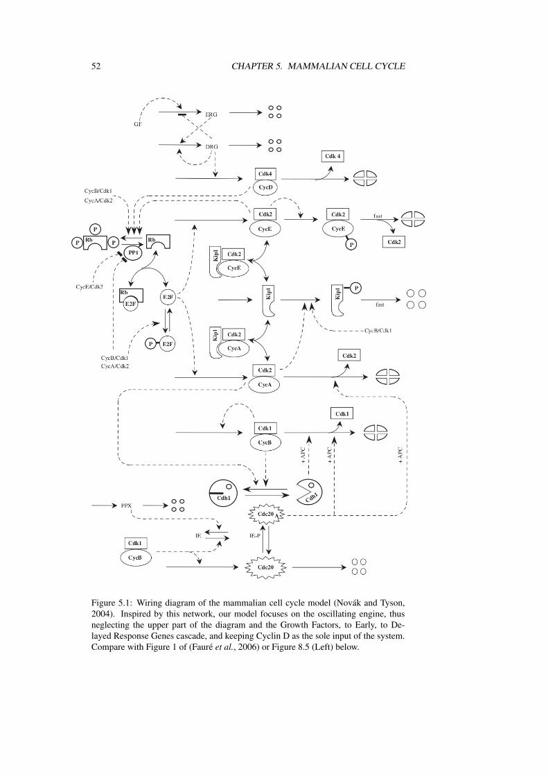
The model we chose as a benchmark for our modelling approach of the cell cyclewas the network controlling the mammalian cell cycle, as proposed by Novák andTyson (2004). According to its authors, this model was a “skeletal” model, basedupon an abstraction of the functionally related proteins composing the real network.The wiring diagram is reproduced in Figure 5.1. Another, much more detailed modelof the budding yeast cell cycle had been published at the same period (Chen et al.,2004), but it was very complex and challenging for a first approach. In contrast, whilesufficiently detailed to be interesting, the mammalian model was sufficiently smallfor its Boolean transcription to be studied under the full asynchronous assumption.Modifications were limited to the introduction of the recently discovered UbcH10(Rape and Kirschner, 2004). This was our first step in the modelling of the cell cycle.
This model is further discussed in Parts 8.2 and 9.2 below.
51
52 CHAPTER 5. MAMMALIAN CELL CYCLE
Figure 5.1: Wiring diagram of the mammalian cell cycle model (Novák and Tyson,2004). Inspired by this network, our model focuses on the oscillating engine, thusneglecting the upper part of the diagram and the Growth Factors, to Early, to De-layed Response Genes cascade, and keeping Cyclin D as the sole input of the system.Compare with Figure 1 of (Fauré et al., 2006) or Figure 8.5 (Left) below.
Vol. 22 no. 14 2006, pages e124–e131
doi:10.1093/bioinformatics/btl210BIOINFORMATICS
Dynamical analysis of a generic Boolean model for the control of
the mammalian cell cycleAdrien Faure, Aurelien Naldi, Claudine Chaouiya and Denis Thieffry�
Institut de Biologie du Developpement de Marseille-Luminy, Campus scientifique de Luminy, CNRS case 907, 13288Marseille, France
ABSTRACT
Motivation: To understand the behaviour of complex biological
regulatory networks, a proper integration of molecular data into a
full-fledge formal dynamical model is ultimately required. As most
available data on regulatory interactions are qualitative, logical mod-
elling offers an interesting framework to delineate the main dynamical
properties of the underlying networks.
Results: Transposing a generic model of the core network controlling
the mammalian cell cycle into the logical framework, we compare
different strategies to explore its dynamical properties. In particular,
we assess the respective advantages and limits of synchronous
versus asynchronous updating assumptions to delineate the asymp-
totical behaviour of regulatory networks. Furthermore, we propose
several intermediate strategies to optimize the computation of asy-
mptotical properties depending on available knowledge.
Availability: The mammalian cell cycle model is available in a
dedicated XML format (GINML) on our website, along with our logical
simulation software GINsim (http://gin.univ-mrs.fr/GINsim). Higher
resolution state transitions graphs are also found on this web site
(Model Repository page).
Contact: [email protected]
1 INTRODUCTION
A proper understanding of the structure and temporal behaviour
of biological regulatory networks requires the integration of
regulatory data into a formal dynamical model (for a review, see
de Jong, 2002). Although this issue has been recurrently addressed
by applying standard mathematical approaches (e.g., differential orstochastic equations) borrowed from physical sciences, it is notably
complicated by the diversity and sophistication of regulatory
mechanisms, as well as by the chronic lack of reliable quantitative
information.
This situation has motivated the development of intrinsically
qualitative approaches leaning on Boolean algebra or generalisation
thereof (Glass & Kauffman, 1973; Thomas, 1991).
In this paper, we lean on previous work refining, extending
and implementing the logical approach initially formulated by
R. Thomas et al. (Thomas, 1991; Thomas et al., 1995). The cor-
responding framework is summarised in the following section (see
Chaouiya et al., 2003, for more detail). This framework is then
used to derive a logical version of the differential model for the
control of the mammalian cell cycle recently published by Novak
and Tyson (2004). The corresponding regulatory network is
described in the last chapter of the introduction, together with
citations of the most relevant experimental articles (for a didactic
introduction to cell cycle modelling, see Fuß et al., 2005).In their landmark model analysis, Novak and Tyson have heavily
relied on numerical integration techniques (temporal simulations,
phase space analyses, and bifurcation diagrams) to delineate the
main dynamical properties of the complex regulatory system under
study. Their results are valid for specific sets of parameter values
and function shapes, which are difficult to establish quantitatively.
Furthermore, such parametric analyses can only handle a few
parameters at once.
In contrast, although much more qualitative, the logical frame-
work enables a more systematic and extensive characterisation of
all the behaviours compatible with a given regulatory graph.
Furthermore, this framework offers enumerative or analytical
means to identify relevant asymptotical behaviours (stable states,
state transition cycles, etc.). Finally, extending a logical model to
encompass additional regulatory modules is relatively easy.
However, one difficulty with the logical approach lies in the
implicit treatment of time. In this respect, different approaches
have been proposed, either considering all transitions under a
synchronicity assumption, or considering them under a fully asyn-
chronous assumption, i.e., selecting a single transition at each
dynamical step. The first assumption is simple but leads to well
known artefacts, whereas the results obtained under the second
assumption are more difficult to evaluate. In this paper, we explore
the use of different strategies enabling a honourable compromise
between these two extreme approaches.
1.1 Logical modelling of regulatory networks
The specification of a logical model involves three main steps:
(i) the building of a regulatory graph; (ii) the definition of the
logical parameters of the system; (iii) the specification of the
updating assumption(s).Cross-regulations between regulatory components are formalized
in terms of an oriented graph. In this regulatory graph, the verticesrepresent the different regulatory components (activity of a gene,
concentration of a regulatory product, or level of activity of a pro-
tein), whereas the edges represent regulatory interactions between
these components (including self-regulations). The level or activity�To whom correspondence should be addressed.
� The Author 2006. Published by Oxford University Press. All rights reserved. For Permissions, please email: [email protected]
The online version of this article has been published under an open access model. Users are entitled to use, reproduce, disseminate, or display the open accessversion of this article for non-commercial purposes provided that: the original authorship is properly and fully attributed; the Journal and Oxford UniversityPress are attributed as the original place of publication with the correct citation details given; if an article is subsequently reproduced or disseminated not in itsentirety but only in part or as a derivative work this must be clearly indicated. For commercial re-use, please contact [email protected]
of a regulatory component i is given by an integer, taking its values
in the interval [0, Maxi], where Maxi is the maximal value consid-
ered for this element (in the simplest, Boolean case,Maxi is set to 1).Each edge is labelled with an interval of integers defining the set of
values for which the source of the interaction influences its target.
Naturally, this interval must be compatible with the values allowed
for the source of the interaction. Furthermore, for sake of simpli-
fication, the maximal value of the interval is usually set to the
maximal value of the source of the interaction (notion of threshold).Note that this definition allows the specification of multiple inter-
actions between two components, provided that each interaction
involves a specific threshold (alternatively, disjoint contiguous
intervals can be used).
Finally, an edge can also be optionally labelled with a positive or
negative sign, which then specifies that the effect of the source on
the target is monotonous, either potentially activating or inhibiting
the target, respectively. The specification of interaction signs only
affects the graphical representation and must be translated into
proper parameter values to obtain coherent regulatory effects.
The next step consists in defining the combinatory effects of the
regulatory inputs on the expression or activity of a given component
of the regulatory graph. The set of inputs is already specified at the
level of the regulatory graph. However, the effect of each regulator
usually depends on the presence of the co-regulators. For the sake
of conciseness, we consider only the combinations of interactions
allowing a significant (non zero, from a logical point of view)
expression or activity of the regulated component. The correspond-
ing logical parameters are each univocally identified by the set of
interactions acting on the regulated genes and take their values in
[1,Maxtarget] (see the next section for a concrete illustration).
The dynamical behaviour of a logical regulatory model is repre-
sented in terms of an oriented graph, where each vertex represents a
specific logical state of the system (i.e., a vector giving the discrete
levels of expression/activity of all the components), whereas the
edges represent (possible) transitions between these states.
Together with the regulatory graph, the logical parameters define
the rules directing the dynamics of a network, i.e., the potential
occurrence of specific edges in the state transition graph. Indeed, ata given state, a specific logical parameter can be associated with
each component. If the value of this parameter is smaller or greater
than that of the concentration/activity level of the corresponding
component, this level will tend to decrease or increase, respectively.
Otherwise (when the parameter value and the corresponding com-
ponent level are equal), the component will tend to keep its current
value.
At this stage, different assumptions might be considered. Accord-
ing to the simplest one, at a given state, all increase or decrease calls
are realized simultaneously (synchronous updating), changing the
component levels by one unit at a time (see e.g., Kauffman, 1993).
Easy to implement and computationally efficient, this approach
leads to well known dynamical artefacts (in particular spurious
cycles). At the other extreme of the spectrum, the transition calls
can be asynchronously updated, i.e., one single transition will be
selected at a time. This assumption requires additional rules to sort
out concurring transitions (e.g., the specification of time delays or of
priorities). These additional rules are tricky to define, as they may
perfectly be context sensitive, i.e., finely depend on the levels of
various regulatory components (although these combinations might
correspond to identical parameter values). For this reason, all
possible transitions are often generated, and an asynchronous tran-sition graph is built where all single possible transitions are con-
sidered, although all resulting dynamical pathways cannot be
followed for a single set of transition rules.
Whatever the updating assumption, of particular interest is the
asymptotical behaviour of the system, e.g., the terminal vertices
(stable states, with no updating calls) or the attractive cycles found
in the state transition graph. Note that such attractors (in particular
the stable states and simple terminal cycles) can easily be located in
the context of the synchronous updating assumption. As we shall
see, the synchronous assumption can often (but not always) be
considered as a shortcut for the computation of the asynchronous
dynamics. This point will be further assessed below through the
analysis of a logical model of the core network controlling the
mammalian cell cycle.
To ease the definition of a regulatory graph and of the associated
logical parameters, as well as the construction of the (a)synchronous
state transition graphs, we have developed a logical modelling/
analysis/simulation software called GINsim (Gonzalez et al.,2006). A new release of GINsim now implements the possibility
to play with the different updating assumptions and to define
different priority classes.Let consider a regulatory graph with n nodes {g1, g2, . . . gn}. A
logical state is a vector S¼(s1, s2, . . . sn) where si is the current levelof the ith regulatory product (si 2 {0, . . .Maxi}). Given such a state,it is possible to determine the evolution of gi, for all i ¼ 1, . . . n.Indeed, given any regulatory component gi, the interactions whichare operating on gi in the state S can be identified, and the relevant
logical parameter (i.e., corresponding to the right combination of
incoming interactions) gives the value ki to which gi should tend. If
si > ki (the current level is greater than the parameter value), there is
a call for decreasing the level of gi, (a decrease call on gi is denotedgi#); if si < ki, there is a call for increasing the level of gi (denotedgi"); otherwise (if si ¼ ki), there is no updating call for this com-
ponent. A stable state is thus a state without updating call.
The synchronicity assumption amounts to apply all concurrent
transitions simultaneously, all states having thus at most one suc-
cessor; under the asynchronous assumption, concurrent transitions
are applied separately, and a state with q updating calls has then
exactly q successors.
Here, we introduce a new functionality of GINsim consisting in
the definition of p priority classes C1, C2, . . . Cp, with p � n, whichgather regulatory products depending on their qualitative pro-
duction and/or degradation delays:
(i) each class Ci is associated with a rank r(Ci) (1� r(Ci)� p, 1
being the highest rank), as well as with an updating policy
(synchronous or asynchronous);
(ii) several classes may have the same rank; and concurrent tran-
sitions on genes of different classes with identical rank are
triggered asynchronously;
(iii) at any state S, among all concurrent transitions, only those on
genes of the classes with the highest rank are triggered;
(iv) concurrent transitions inside a class are triggered accordingly
to the updating policy associated to that class;
(v) finally, increasing and decreasing transitions of each gene
can be distinguished and associated to classes with different
ranks.
Dynamical analysis of a generic Boolean model for the control of the mammalian cell cycle
e125
1.2 Regulation of the mammalian cell cycle
The cell cycle involves a succession of molecular events leading to
the reproduction of the genome of a cell (Synthesis or S phase) and
its division into two daughter cells (Mitosis, or M phase). The M
phase itself encompasses different sub-phases (prophase, meta-
phase, anaphase, telophase) characterised by specific chromosomal
and nuclear changes (respectively: condensation of the chromatin,
alignment of the chromosomes, separation of the sister chromatids,
and formation of the two daughter nuclei). The S and M phases are
preceded by two gap phases, called G1 and G2 respectively (for a
review, see, for example, Tessema et al., 2004). These events
are very well known and can easily be monitored with an optical
microscope.
During the late 1970s and early 1980s, yeast geneticists have
identified the cell-division-cycle (cdc) genes, encoding for new
classes of molecules including the cyclins (so called because of
their cyclic pattern of activation), and their cyclin dependent
kinases (cdk) partners. Since then, our knowledge of the molecular
network that controls cell cycle events has tremendously pro-
gressed, but the number of components and interactions known
to be involved has so much increased that proper formal modelling
becomes necessary to understand the behaviour of such a
complex system.
Our model analysis is rooted in the seminal work of Novak
and Tyson, who have recently derived and analyzed a set of 18
ordinary differential equations (ODE) to model the control of the
restriction point of the mammalian cell cycle (Novak and Tyson,
2004). Based on this differential model and using numerical inte-
gration techniques, the authors were able to qualitatively reproduce
the main known dynamical features of the wild-type biological
system, as well as the consequences of several types of perturba-
tions. This state-of-the-art model study nevertheless appears diffi-
cult to extend, although there is clearly many more regulators,
variants and interactions to consider (see, e.g., Kohn’s map at
http://discover.nci.nih.gov/kohnk/fig6a.html).
In this respect, the logical formalism offers an appropriate
framework to qualitatively explore the dynamical properties of
relatively complex regulatory graphs. However, up to now, it has
been mostly applied to transcriptional regulatory networks, and its
application to the numerous and various protein interactions at the
core of the cell cycle network was thus a challenge.
As a starting point, we have used Novak and Tyson’s diagram
and model to build a logical regulatory graph (see Figure 1). In the
process, we were led to derive a proper logical representation for
each type of regulatory interaction. In what follows, we summarize
the main experimental data and assumptions underlying our
regulatory graph. In the context of this paper, we further focus
on a specific Boolean version of this model.
Mammalian cell division is tightly controlled, for it must be
coordinated with the overall growth of the organism, as well as
answer specific needs, such as wound healing for example.
This coordination is achieved through extra-cellular positive and
negative signals whose balance decides whether a cell will divide or
remain in a resting state (quiescence or G0 phase), which can be
reached and left by the cell during the G1 phase. The positive
signals or growth factors ultimately elicit the activation of
Cyclin D in the cell. In our model, CycD thus represents the
input, and its activity is considered constant. Note that cdk4 and
cdk6, the partners of Cyclin D, are not explicitly represented in our
model, for their activity essentially depends on the presence or
absence of their cyclin. In other words, CycD stands here for the
whole cdk4/6-Cyclin D complex. The same approach has been
adopted for the other cyclin/cdk pairs.
In our model, CycD is necessary for the inactivation of the
retinoblastoma protein Rb, and for the sequestration of p27/Kip1
(p27 in the sequel). This protein is a cdk inhibitor that sequesters
cdk2/Cyclin E (CycE) and cdk2/Cyclin A (CycA), preventing
them from phosphorylating their targets (reviewed in Coqueret,
2003). It is usually considered that Cyclin D remains active
when in complex with p27, though the issue is still debated
(Olashaw et al., 2004). For the sake of simplicity, we consider
that CycD directly inhibits p27.
In contrast, the complexes formed by p27 and CycE or CycA
are represented in a subtler way, though this formation remains
implicit: when both p27 and CycE or CycA are active, the complex
forms, and the activity of the cyclin is blocked. To model the fact
that the cyclins remain present though sequestered when linked to
p27, we consider that p27 opposes their activities on their targets,
instead of directly inhibiting them. In our model, this is embodied
by arrows from p27 onto the targets of CycE and CycA, with a sign
opposite to that corresponding to the effect of the cyclins on their
targets in the absence of p27.
The other target of CycD, Rb, is a key tumour suppressor,
which is found mutated in a large variety of cancers. Rb is inac-
tivated by phosphorylation, and CycD is involved in the first step of
this process (reviewed in Tamrakar et al., 2000). However, in this
simplified Boolean model, we consider that Rb inactivation by
CycD is total.
Rb forms a complex with members of the E2F family of
transcription factors, turning them from transcriptional activators
to repressors, in part through recruitment of chromatin remodelling
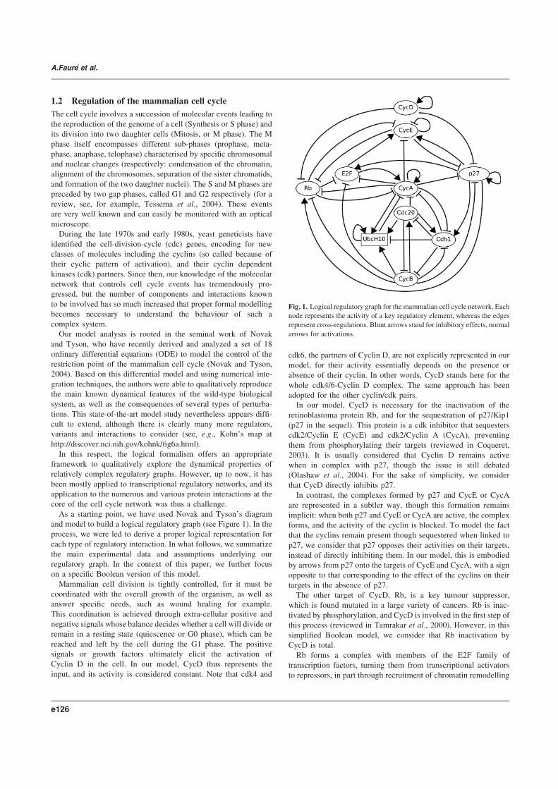
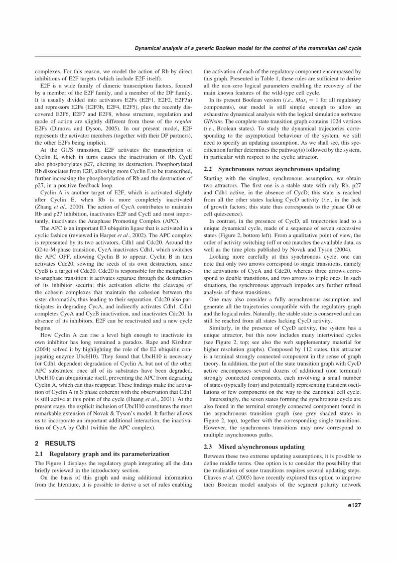
Fig. 1. Logical regulatory graph for the mammalian cell cycle network. Each
node represents the activity of a key regulatory element, whereas the edges
represent cross-regulations. Blunt arrows stand for inhibitory effects, normal
arrows for activations.
A.Faure et al.
e126
complexes. For this reason, we model the action of Rb by direct
inhibitions of E2F targets (which include E2F itself).
E2F is a wide family of dimeric transcription factors, formed
by a member of the E2F family, and a member of the DP family.
It is usually divided into activators E2Fs (E2F1, E2F2, E2F3a)
and repressors E2Fs (E2F3b, E2F4, E2F5), plus the recently dis-
covered E2F6, E2F7 and E2F8, whose structure, regulation and
mode of action are slightly different from those of the regularE2Fs (Dimova and Dyson, 2005). In our present model, E2F
represents the activator members (together with their DP partners),
the other E2Fs being implicit.
At the G1/S transition, E2F activates the transcription of
Cyclin E, which in turns causes the inactivation of Rb. CycE
also phosphorylates p27, eliciting its destruction. Phosphorylated
Rb dissociates from E2F, allowing more Cyclin E to be transcribed,
further increasing the phosphorylation of Rb and the destruction of
p27, in a positive feedback loop.
Cyclin A is another target of E2F, which is activated slightly
after Cyclin E, when Rb is more completely inactivated
(Zhang et al., 2000). The action of CycA contributes to maintain
Rb and p27 inhibition, inactivates E2F and CycE and most impor-
tantly, inactivates the Anaphase Promoting Complex (APC).
The APC is an important E3 ubiquitin ligase that is activated in a
cyclic fashion (reviewed in Harper et al., 2002). The APC complex
is represented by its two activators, Cdh1 and Cdc20. Around the
G2-to-M-phase transition, CycA inactivates Cdh1, which switches
the APC OFF, allowing Cyclin B to appear. Cyclin B in turn
activates Cdc20, sowing the seeds of its own destruction, since
CycB is a target of Cdc20. Cdc20 is responsible for the metaphase-
to-anaphase transition: it activates separase through the destruction
of its inhibitor securin; this activation elicits the cleavage of
the cohesin complexes that maintain the cohesion between the
sister chromatids, thus leading to their separation. Cdc20 also par-
ticipates in degrading CycA, and indirectly activates Cdh1. Cdh1
completes CycA and CycB inactivation, and inactivates Cdc20. In
absence of its inhibitors, E2F can be reactivated and a new cycle
begins.
How Cyclin A can rise a level high enough to inactivate its
own inhibitor has long remained a paradox. Rape and Kirshner
(2004) solved it by highlighting the role of the E2 ubiquitin con-
jugating enzyme UbcH10). They found that UbcH10 is necessary
for Cdh1 dependent degradation of Cyclin A, but not of the other
APC substrates; once all of its substrates have been degraded,
UbcH10 can ubiquitinate itself, preventing the APC from degrading
Cyclin A, which can thus reappear. These findings make the activa-
tion of Cyclin A in S phase coherent with the observation that Cdh1
is still active at this point of the cycle (Huang et al., 2001). At thepresent stage, the explicit inclusion of UbcH10 constitutes the most
remarkable extension of Novak & Tyson’s model. It further allows
us to incorporate an important additional interaction, the inactiva-
tion of CycA by Cdh1 (within the APC complex).
2 RESULTS
2.1 Regulatory graph and its parameterization
The Figure 1 displays the regulatory graph integrating all the data
briefly reviewed in the introductory section.
On the basis of this graph and using additional information
from the literature, it is possible to derive a set of rules enabling
the activation of each of the regulatory component encompassed by
this graph. Presented in Table 1, these rules are sufficient to derive
all the non-zero logical parameters enabling the recovery of the
main known features of the wild-type cell cycle.
In its present Boolean version (i.e., Maxi ¼ 1 for all regulatory
components), our model is still simple enough to allow an
exhaustive dynamical analysis with the logical simulation software
GINsim. The complete state transition graph contains 1024 vertices
(i.e., Boolean states). To study the dynamical trajectories corre-
sponding to the asymptotical behaviour of the system, we still
need to specify an updating assumption. As we shall see, this spe-
cification further determines the pathway(s) followed by the system,
in particular with respect to the cyclic attractor.
2.2 Synchronous versus asynchronous updating
Starting with the simplest, synchronous assumption, we obtain
two attractors. The first one is a stable state with only Rb, p27
and Cdh1 active, in the absence of CycD; this state is reached
from all the other states lacking CycD activity (i.e., in the lack
of growth factors; this state thus corresponds to the phase G0 or
cell quiescence).
In contrast, in the presence of CycD, all trajectories lead to a
unique dynamical cycle, made of a sequence of seven successive
states (Figure 2, bottom left). From a qualitative point of view, the
order of activity switching (off or on) matches the available data, as
well as the time plots published by Novak and Tyson (2004).
Looking more carefully at this synchronous cycle, one can
note that only two arrows correspond to single transitions, namely
the activations of CycA and Cdc20, whereas three arrows corre-
spond to double transitions, and two arrows to triple ones. In such
situations, the synchronous approach impedes any further refined
analysis of these transitions.
One may also consider a fully asynchronous assumption and
generate all the trajectories compatible with the regulatory graph
and the logical rules. Naturally, the stable state is conserved and can
still be reached from all states lacking CycD activity.
Similarly, in the presence of CycD activity, the system has a
unique attractor, but this now includes many intertwined cycles
(see Figure 2, top; see also the web supplementary material for
higher resolution graphs). Composed by 112 states, this attractor
is a terminal strongly connected component in the sense of graph
theory. In addition, the part of the state transition graph with CycD
active encompasses several dozens of additional (non terminal)
strongly connected components, each involving a small number
of states (typically four) and potentially representing transient oscil-
lations of few components on the way to the canonical cell cycle.
Interestingly, the seven states forming the synchronous cycle are
also found in the terminal strongly connected component found in
the asynchronous transition graph (see grey shaded states in
Figure 2, top), together with the corresponding single transitions.
However, the synchronous transitions may now correspond to
multiple asynchronous paths.
2.3 Mixed a/synchronous updating
Between these two extreme updating assumptions, it is possible to
define middle terms. One option is to consider the possibility that
the realisation of some transitions requires several updating steps.
Chaves et al. (2005) have recently explored this option to improve
their Boolean model analysis of the segment polarity network
Dynamical analysis of a generic Boolean model for the control of the mammalian cell cycle
e127
involved in the segmentation of the trunk of Drosophila embryos.
Here, we propose an alternative approach enabling the combination
of synchronous and asynchronous assumptions depending on the
regulatory element or on the nature of transition considered. Indeed,
depending on available knowledge or on the biological questions
addressed, it may be necessary to go into fine grain dynamical
analysis for only a subset of regulatory components. To deal
with these issues, the last version of GINsim enables the user to
group components into different classes, and to assign a prioritylevel to each of these classes. In case of concurrent transition calls,
GINsim first updates the gene(s) belonging to the class with the
highest ranking. For each regulatory component class, the user can
further specify the desired updating assumption, which then deter-
mines the treatment of concurrent transition calls inside that class.
When several classes have the same ranking, concurrent transitions
are treated under an asynchronous assumption (no priority).
To illustrate this approach, we have first built two priority classes,
which arguably group faster versus slower biochemical processes.
In the highest ranked transition priority class, we have included the
degradations of E2F, CycE, CycA, Cdc20, UbcH10, CycB, as well
as all transitions (in both directions) for CycD, Rb, p27 (Kip1) and
Cdh1. The remaining transitions corresponding to synthesis rates (of
E2F, CycE, CycA, Cdc20, UbcH10, and CycB) are grouped in a
lower priority class. Using these two priority classes, both consid-
ered under the asynchronous assumption, we still obtain a single
terminal strongly connected component (not shown) involving 34
states (to compare with the seven states obtained with the standard
synchronous treatment, versus the 112 states in the fully asyn-
chronous case without priority).
The analysis of this component reveals that some pathways are
clearly unrealistic, as they skip the activation of some crucial
cyclins, for example. To eliminate these spurious pathways, one
can further refine the priority classes, taking into account additional
information. Here, we can exploit the fact that several transitions are
controlled by similar regulatory mechanisms and group them
into synchronous classes. This leads to the definition of the four
transition classes displayed in Table 2.
For this last prioritisation, we obtain a smaller terminal strongly
connected component involving 18 states, which combine single
and multiple transitions. This mixed graph is thus much simpler that
the fully asynchronous transition graph. This graph enables a finer
description of the sequence of events characteristic of the normal
cell cycle than in the fully synchronous case. However, the data
presently available do not allow a clear distinction between the
different alternative pathways.
2.4 Mutant simulations
Beyond a faithful reproduction of the wild-type behaviour, a good
cell cycle model should enable the simulation of various types of
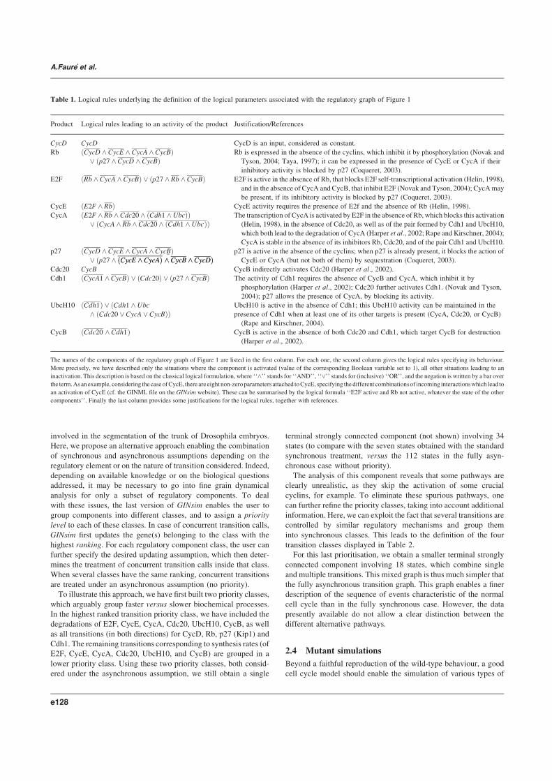
Table 1. Logical rules underlying the definition of the logical parameters associated with the regulatory graph of Figure 1
Product Logical rules leading to an activity of the product Justification/References
CycD CycD CycD is an input, considered as constant.
Rb ðCycD ^ CycE ^ CycA ^ CycBÞ_ ðp27 ^ CycD ^ CycBÞ
Rb is expressed in the absence of the cyclins, which inhibit it by phosphorylation (Novak and
Tyson, 2004; Taya, 1997); it can be expressed in the presence of CycE or CycA if their
inhibitory activity is blocked by p27 (Coqueret, 2003).
E2F ðRb ^ CycA ^ CycBÞ _ ðp27 ^ Rb ^ CycBÞ E2F is active in the absence of Rb, that blocks E2F self-transcriptional activation (Helin, 1998),
and in the absence of CycA and CycB, that inhibit E2F (Novak and Tyson, 2004); CycAmay
be present, if its inhibitory activity is blocked by p27 (Coqueret, 2003).
CycE ðE2F ^ RbÞ CycE activity requires the presence of E2f and the absence of Rb (Helin, 1998).
CycA ðE2F ^ Rb ^ Cdc20 ^ ðCdh1 ^ UbcÞÞ_ ðCycA ^ Rb ^ Cdc20 ^ ðCdh1 ^ UbcÞÞ
The transcription of CycA is activated by E2F in the absence of Rb, which blocks this activation
(Helin, 1998), in the absence of Cdc20, as well as of the pair formed by Cdh1 and UbcH10,
which both lead to the degradation of CycA (Harper et al., 2002; Rape and Kirschner, 2004);
CycA is stable in the absence of its inhibitors Rb, Cdc20, and of the pair Cdh1 and UbcH10.
p27 ðCycD ^ CycE ^ CycA ^ CycBÞ_ ðp27 ^ �ðCycE ^ CycAÞ ^ CycB ^ CycDÞðCycE ^ CycAÞ ^ CycB ^ CycDÞ
p27 is active in the absence of the cyclins; when p27 is already present, it blocks the action of
CycE or CycA (but not both of them) by sequestration (Coqueret, 2003).
Cdc20 CycB CycB indirectly activates Cdc20 (Harper et al., 2002).
Cdh1 ðCycA1 ^ CycBÞ _ ðCdc20Þ _ ðp27 ^ CycBÞ The activity of Cdh1 requires the absence of CycB and CycA, which inhibit it by
phosphorylation (Harper et al., 2002); Cdc20 further activates Cdh1. (Novak and Tyson,
2004); p27 allows the presence of CycA, by blocking its activity.
UbcH10 ðCdh1Þ _ ðCdh1 ^ Ubc
^ ðCdc20 _ CycA _ CycBÞÞUbcH10 is active in the absence of Cdh1; this UbcH10 activity can be maintained in the
presence of Cdh1 when at least one of its other targets is present (CycA, Cdc20, or CycB)
(Rape and Kirschner, 2004).
CycB ðCdc20 ^ Cdh1Þ CycB is active in the absence of both Cdc20 and Cdh1, which target CycB for destruction
(Harper et al., 2002).
components’’. Finally the last column provides some justifications for the logical rules, together with references.
The names of the components of the regulatory graph of Figure 1 are listed in the first column. For each one, the second column gives the logical rules specifying its behaviour.
More precisely, we have described only the situations where the component is activated (value of the corresponding Boolean variable set to 1), all other situations leading to an
inactivation. This description is based on the classical logical formulation, where ‘‘^’’ stands for ‘‘AND’’, ‘‘_’’ stands for (inclusive) ‘‘OR’’, and the negation is written by a bar overthe term.As anexample, considering the case ofCycE, there are eight non-zeroparameters attached toCycE, specifying thedifferent combinationsof incoming interactionswhich lead to
an activation of CycE (cf. the GINML file on the GINsim website). These can be summarised by the logical formula ‘‘E2F active and Rb not active, whatever the state of the other
A.Faure et al.
e128
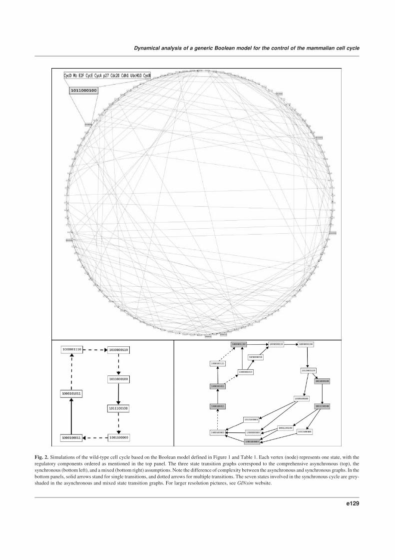
Fig. 2. Simulations of the wild-type cell cycle based on the Boolean model defined in Figure 1 and Table 1. Each vertex (node) represents one state, with the
regulatory components ordered as mentioned in the top panel. The three state transition graphs correspond to the comprehensive asynchronous (top), the
synchronous (bottom left), and amixed (bottom right) assumptions. Note the difference of complexity between the asynchronous and synchronous graphs. In the
bottom panels, solid arrows stand for single transitions, and dotted arrows for multiple transitions. The seven states involved in the synchronous cycle are grey-
shaded in the asynchronous and mixed state transition graphs. For larger resolution pictures, see GINsim website.
Dynamical analysis of a generic Boolean model for the control of the mammalian cell cycle
e129
perturbations, in particular, the addition of drugs interfering with
cell growth or cyclin activities, or the presence of loss-of-function
or gain-of-function mutations in some of the core regulatory genes.
In this respect, GINsim provides a simple interface to constraint
selected regulatory components within specific value intervals.
Depending on the initial state(s), once a regulatory component
has reached the corresponding value interval in the course of the
simulation, all transitions leading outside of this interval are
automatically discarded. This function greatly eases the simula-
tion of loss-of-function and gain-of-function mutants (a table
compiling our mutant analyses is maintained on the GINsim web
page). As we have represented molecule families by single com-
ponents, the comparison between in silico and experimental
results are not always straightforward. However, up to now, all
our simulation results are consistent with available experimental
data (loss versus preservation of cell cycle depending on the mutant
considered), but a few exceptions like the case of the p27 loss-of-
function, for which our model predicts a stable state in the absence
of CycD, whereas published data support the existence of oscilla-
tions in this situation. This discrepancy is likely due to the crude
representation of CycE and Rb activity levels in terms of Boolean
variables and could be solved by using ternary variables for these
elements.
3 CONCLUSIONS AND PROSPECTS
In this paper, we have assessed the power of the logical approach,
already in its simplest Boolean form, for the modelling of a complex
protein interaction network. We have further presented extensions
of our software GINsim to enable detailed studies of the asymptoti-
cal behaviour of complex systems, with synchronous, asynchronous
or mixed treatment of concurrent transitions.
As shown through the analysis of a model for the mammalian cell
cycle, a relatively simple logical model captures most qualitative
dynamical features of the wild-type network, as well as of docu-
mented mutants. Strikingly, even simplistic synchronous simula-
tions give rise to (only) two attractors consistent with available data,
as well as with the simulations of Novak and Tyson (2004). On the
one hand, we obtain a stable state in the absence of CycD, which
matches our knowledge of quiescent cellular states when growth
factors are lacking. On the other hand, in the presence of CycD, all
trajectories converge towards a unique complex dynamical cycle.
This is a favourable situation for the synchronous assumption, as no
spurious cycle is generated.
However, the synchronous dynamics obtained does not allow
the temporal separation of multiple regulatory activity changes.
In contrast, asynchronous updating does allow finer temporal
analyses, but the resulting state transition graph is very complex
and encompasses many incompatible or unrealistic pathways. Lean-
ing on specific GINsim functions, we have thus considered system-
atic ways to combine synchronous and asynchronous transitions,
taking advantage of existing information on kinetics or regulatory
mechanisms. This application thus illustrates the flexibility of the
combination of different updating assumptions.
The logical formalism used should further enable the identifica-
tion of the regulatory circuits playing the most crucial dynamical
roles (Thomas et al., 1995). Our present model comprises 132
different circuits, involving from one to nine regulatory elements.
A preliminary analysis suggests that only a dozen of these circuits
are functional in some region of the variable space, most of the time
only in the absence of CycD. The precise role of these different
circuits has still to be clarified.
Modelling the molecular regulatory network controlling
mammalian cell cycle is clearly a challenging and long-term enter-
prise. Focusing on the core network controlling the mammalian cell
cycle, our present Boolean model corresponds to a relatively high
level abstraction of our knowledge of the cellular system, which
involves many variants for several of the molecular species
considered (E2F, RB. . .). In this respect, the generation of extensivefunctional genomics data sets should prove of great help to delineate
the specific expression and interaction patterns of these variants
(for a pioneering attempt to exploit various kinds of functional
genomic data sets to dynamically characterise the molecular net-
work controlling the cell cycle in yeast, see the recent article by de
Lichtenberg et al., 2005). On the basis of our generic, abstract
model, several extensions or refinements can now be considered,
including the use of multilevel variables wherever biological jus-
tifications can be advanced, further specifications and enrichments
of this model in reference to specific cell types, or yet the inclusion
of additional control modules.
A substantial increase in the sophistication of the logical
models considered will lead to combinatorial problems, e.g., toidentify all attractors or to analyze the trajectories leading to
these attractors. To prepare the ground to deal with such combina-
torial problems, we are exploring different approaches. First, we use
constraint programming to delineate attractors from simple or
composed logical models without computing the whole state tran-
sition graph (Devloo et al., 2003). Next, we have developed and
implemented a set of translations rules enabling the export of
parameterised regulatory graphs into standard or coloured
Petri nets, thereby enabling the use of the various dynamical anal-
ysis tools developed by this lively community (Chaouiya et al., inpress). Finally, we are presently evaluating the application of
temporal logic formalisms (e.g., Computational Tree Logics) to
assess the existence of specific dynamical pathways, or to
encompass specific temporal information (Bernot et al., 2004;
Batt et al., 2005).Ultimately, more quantitative models are needed to explore fine
grain aspects of the control of the cell cycle, e.g., modulations of the
cycle period or of its amplitude. In this respect, Petri nets constitute
an interesting framework to refine discrete models, leaning on exist-
ing hybrid or stochastic extensions. Alternatively, one may use sets
of differential or stochastic equations, but even in this case, a
preparatory logical analysis should prove useful when dealing
with large and complex regulatory networks.
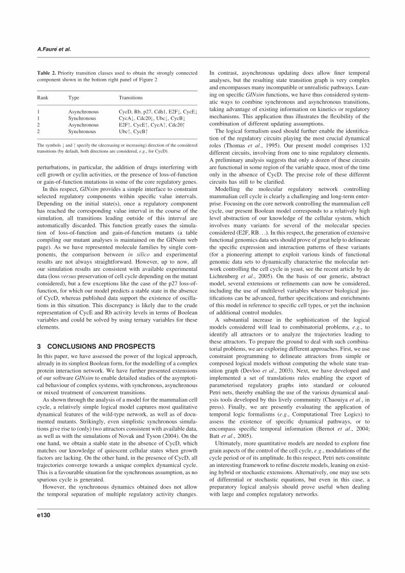
Table 2. Priority transition classes used to obtain the strongly connected
component shown in the bottom right panel of Figure 2
Rank Type Transitions
1 Asynchronous CycD, Rb, p27, Cdh1, E2F#, CycE#1 Synchronous CycA#, Cdc20#, Ubc#, CycB#2 Asynchronous E2F", CycE", CycA", Cdc20"2 Synchronous Ubc", CycB"
The symbols # and " specify the (decreasing or increasing) direction of the considered
transitions (by default, both directions are considered, e.g., for CycD).
A.Faure et al.
e130
ACKNOWLEDGEMENTS
We wish to thank A. Ciliberto and K. Helin, as well as E. Remy,
P. Ruet and B. Mosse, for insightful discussions on biological, and
mathematical aspects of this work. We acknowledge financial
support from the European Commission (contract LSHG-CT-
2004-512143), the French Research Ministry (ACI IMPbio), the
CNRS, and the INRIA (ARC MOCA).
REFERENCES
Batt,G., Ropers,D., de Jong,H., Geiselmann,J., Mateescu,R., Page,M., Schneider,D.
(2005) Validation of qualitative models of genetic regulatory networks by model
checking: analysis of the nutritional stress response in Escherichia coli.
Bioinformatics, 21, i19–i28.
Bernot,G., Comet,J.P., Richard,A., Guespin,J. (2004) Application of formal
methods to biological regulatory networks: extending Thomas’ asynchronous
logical approach with temporal logic. J. Theor. Biol., 229, 339–347.
Chaouiya,C., Remy,E., Mosse,B., Thieffry,D. (2003) Qualitative analysis of
regulatory graphs: A computational tool based on a discrete formal framework.
Lect. Notes Control Inf. Sci., 294, 119–126.
Chaouiya,C., Remy,E., Thieffry,D. (in press) Petri net modelling of biological
regulatory networks. J. Discrete Algorithms.
Chaves,M., Albert,R., Sontag,E.D. (2005) Robustness and fragility of Boolean
models for genetic regulatory networks. J. Theor. Biol., 235, 431–449.
Coqueret,O. (2003) New roles for p21 and p27 cell-cycle inhibitors: a function for each
cell compartment? Trends Cell Biol., 13, 65–70.
de Jong,H. (2002) Modelling and simulation of genetic regulatory systems: A literature
review. J. Comput. Biol., 9, 67–103.
de Lichtenberg,U., Jensen,L.J., Brunak,S., Bork,P. (2005) Dynamic complex formation
during the yeast cell cycle. Science, 307, 724–727.
Devloo,V., Hansen,P., Labbe,M. (2003) Identification of all steady states in large
networks by logical analysis. Bull. Math. Biol., 65, 1025–1051.
Dimova,D.K., Dyson,N.J. (2005) The E2F transcriptional network: old acquaintances
with new faces. Oncogene, 24, 2810–2826.
Fuß,H., Dubitzky,W., Downes,C.S., Kurth,M.J. (2005) Mathematical models of cell
cycle regulation. Brief. Bioinformatics, 6, 163–177.
Glass,L., Kauffman,S.A. (1973) The logical analysis of continuous non-linear
biochemical control networks. J. Theor. Biol., 39, 103–129.
Gonzalez,A.G., Naldi A.,Sanchez,L., Thieffry,D., Chaouiya,C. (2006) GINsim: a soft-
ware suite for the qualitative modelling, simulation and analysis of regulatory
networks. Biosystems, 84, 91–100.
Harper,J.W., Burton,J.L., Solomon,M.J. (2002) The anaphase-promoting complex: it’s
not just for mitosis anymore. Genes Dev., 16, 2179–2206.
Helin,K. (1998). Regulation of cell proliferation by the E2F transcription factors.
Curr. Opin. Genet. Dev., 8, 28–35.
Huang,J.N., Park,I., Ellingson,E., Littlepage,L.E., Pellman,D. (2001) Activity of
the APCCdh1 form of the anaphase-promoting complex persists until S phase
and prevents the premature expression of Cdc20p. J. Cell Biol., 154, 85–94.
Kauffman,S.A. (1993) The Origins of Order: Self-Organization and Selection in
Evolution. Oxford University Press.
Novak,B., Tyson,J.J. (2004) A model for restriction point control of the mammalian
cell cycle. J. Theor. Biol., 230, 563–579.
Olashaw,N., Bagui,T.K., Pledger,W.J. (2004) Cell Cycle Control A Complex Issue.
Cell Cycle, 3, 263–264.
Rape,M., Kirshner,W.W. (2004) Autonomous regulation of the anaphase-promoting
complex couples mitosis to S-phase entry. Nature, 432, 588–595.
Tamrakar,S., Rubin,E., Ludlow,J.W. (2000) Role of pRb dephosphorylation in cell
cycle regulation. Front. Biosci., 5, 121–137.
Taya,Y. (1997) RB kinases and RB-binding proteins: new points of view. Trends
Biochem. Sci., 22, 14–17.
Tessema,M., Lehmann,U., Kreipe,H. (2004) Cell cycle and no end. Virchows Arch.,
444, 313–323.
Thomas,R. (1991) Regulatory networks seen as asynchronous automata: a logical
description. J. Theor. Biol., 153, 1–23.
Thomas,R., Thieffry,D., Kaufman,M. (1995) Dynamical behaviour of biological
regulatory networks—I. Biological role of feedback loops and practical use
of the concept of the loop-characteristic state. Bull. Math. Biol., 57,247–276.
Zhang,H.S., Gavin,M., Dahiya,A., Postigo,A.A., Ma,D., Luo,R.X., Harbour,J.W.,
Dean,D.C. (2000) Exit from G1 and S phase of the cell cycle is regulated
by repressor complexes containing HDAC-Rb-hSWI/SNF and Rb-hSWI/SNF.
Cell, 101, 79–89.
Dynamical analysis of a generic Boolean model for the control of the mammalian cell cycle
e131