malthus to modernity: england’s first fertility transition ... to modernity...cambridge group...
TRANSCRIPT

Malthus to Modernity: England’s First Fertility Transition, 1760-1800
Gregory Clark, Department of Economics, University of California, Davis ([email protected])
Neil Cummins, Department of Economics, Queens College, CUNY ([email protected])
August 30, 2012
A key element in developing unified theories of long-run economic growth has been linking the onset of modern growth with the move to modern fertility limitation. A notable puzzle for these theories is that modern growth in England began around 1780, 100 years before there was seemingly any movement to limit fertility. Here we show that the aggregate data on fertility in England before 1890 conceals significant declines in the fertility of the middle and upper classes ear-lier. These declines coincide exactly with the Industrial Revolution. There is a remaining puzzle, however, as to whether these changes represented a response to changing economic conditions.
Two events created the modern economic world: the Industrial Revolution and the Demographic Transition. The Industrial Revolution increased the growth rate of output through a stream of innovations. But as important was the Demographic Transition. In the Malthusian regime that characterized most pre-industrial societies before 1800, there was some technological advance, though slow and spasmodic. But all technological advance was absorbed in raising the stock of people, not in raising living standards. Since fertility increased with income, any rise in living standards induced population growth. Technological gains were consumed in maintaining ever larger populations. But for the Demographic Transition much of modern growth would similarly have been absorbed in maintaining ever greater population levels. High modern incomes in developed countries are thus the joint product of these two revolutions.

2
Figure 1: Net fertility trends in England, 1540s-1910s
Sources: Five year averages for 1541-1871 taken from Wilson 1991. After 1871, decadal averages are taken from Coale and Treadway 1986. The Industrial Revolution, however, dates to 1760-1800, while the Demographic Transition in England occurred around 1890.1 There is at least a 100 year gap between these two events. Figure 1, for example, shows marital fertility in England, estimated to be largely unchanged until 1890 and later. Marriage rates, if anything, increase during the Industrial Revolution. The basic elements of fertility thus seem unchanged until 1890 and later. The Industrial Revolution itself is instead associated with unprecedentedly fast population growth in England. These gross facts of population have led historians and demographers to focus on 1890 as the key and only break in English demographic history. They have also created a problem for
1Taking the Demographic Transition as the date overall marital fertility fell by 10%.
0
0.1
0.2
0.3
0.4
0.5
0.6
0.7
0.8
1540 1580 1620 1660 1700 1740 1780 1820 1860 1900
Fert
ility
Indi
ces
Marital Fertility
Marriage Rate
Total Fertility

3
theories which seek to explain modern growth through a shift from child quantity to child quality.2 The arrival of sustained technological advance clearly long preceded the Demographic Transition. We show using evidence from men’s wills that, starting with the generation marrying in the 1760s, there were in fact significant declines in net fertility in Indus-trial Revolution England, preceding the aggregate decline by over a century, but only among the middle and upper classes. Around 1800 rich men switched from a net fertility of above 4 children, to one of 3 or less, no different than the general popula-tion. This large change in behavior does not show in the aggregate English data because at the same time the net fertility of poorer groups, the bulk of the society, increased to equal that of the rich. Thus by the time of the onset of the second fertility transition in 1880-1910 the net fertility of the poor equaled that of the rich. The limited and contradictory earlier evidence on the relationship between wealth and fertility in pre-industrial England, and the fact that marriage ages and nuptuality were seemingly similar in 1850 to their earlier levels of many decades, created a false impression that the fertility regime of the mid nineteenth century, where fertility differed little by social class, represented the entire pre-industrial
period.3 However, Clark and Hamilton, 2006, using the methods employed here showed that the net fertility of the wealthy was nearly twice that of the society as a whole in England in the seventeenth century. Supporting this in seventeenth century London infant death rates were substantially higher in poorer parishes (Landers, 1993, 186-88). And studies of a parish in Lancashire (Hughes, 1986), and another in Cumbria (Scott and Duncan, 2000), similarly identify a positive relationship between both gross and net fertility and wealth in 1600-1800. A recent study that uses the Cambridge Group Parish reconstitution data find significant fertility differences by occupational status before 1750 (Boberg-Fazlic, Sharp, and Weisdorf, 2011). 4
2 Becker, Murphy and Tamura, 1990, Galor and Weil, 2000, Galor and Moav, 2002, Hansen and Prescott, 2002, Lucas, 2002. 3 Hollingsworth showed that from 1350-1729 the net fertility of the richest of English ducal families, was generally below the average for England (Hollingsworth, 1965). Wrigley and his associates concluded that fertility differentials by occupation were “trivial” before 1837 (Wrigley et al., 1997, 427). 4 This parish record analysis finds more muted effects than here, but this is because occupa-tions are imperfect measures of wealth, wealth itself being the crucial explanator of fertility before 1760 as we shall see below.

4
Thus there must have been a transition between the pre-industrial regime of a strong positive correlation of fertility with wealth and occupational status, and the nineteenth century pre-demographic transition regime where fertility was similar across social and wealth classes. Despite many years of research into the demogra-phy of pre-industrial England we seem to have missed an earlier substantial trans-formation in the demographic system that accompanied the Industrial Revolution.
5
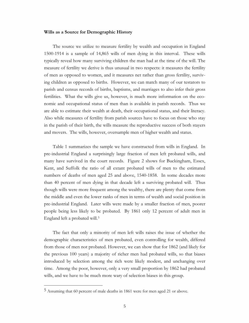
Wills as a Source for Demographic History The source we utilize to measure fertility by wealth and occupation in England 1500-1914 is a sample of 14,865 wills of men dying in this interval. These wills typically reveal how many surviving children the man had at the time of the will. The measure of fertility we derive is thus unusual in two respects: it measures the fertility of men as opposed to women, and it measures net rather than gross fertility, surviv-ing children as opposed to births. However, we can match many of our testators to parish and census records of births, baptisms, and marriages to also infer their gross fertilities. What the wills give us, however, is much more information on the eco-nomic and occupational status of men than is available in parish records. Thus we are able to estimate their wealth at death, their occupational status, and their literacy. Also while measures of fertility from parish sources have to focus on those who stay in the parish of their birth, the wills measure the reproductive success of both stayers and movers. The wills, however, oversample men of higher wealth and status. Table 1 summarizes the sample we have constructed from wills in England. In pre-industrial England a surprisingly large fraction of men left probated wills, and many have survived in the court records. Figure 2 shows for Buckingham, Essex, Kent, and Suffolk the ratio of all extant probated wills of men to the estimated numbers of deaths of men aged 25 and above, 1540-1858. In some decades more than 40 percent of men dying in that decade left a surviving probated will. Thus though wills were more frequent among the wealthy, there are plenty that come from the middle and even the lower ranks of men in terms of wealth and social position in pre-industrial England. Later wills were made by a smaller fraction of men, poorer people being less likely to be probated. By 1861 only 12 percent of adult men in England left a probated will.5
The fact that only a minority of men left wills raises the issue of whether the demographic characteristics of men probated, even controlling for wealth, differed from those of men not probated. However, we can show that for 1862 (and likely for the previous 100 years) a majority of richer men had probated wills, so that biases introduced by selection among the rich were likely modest, and unchanging over time. Among the poor, however, only a very small proportion by 1862 had probated wills, and we have to be much more wary of selection biases in this group.
5 Assuming that 60 percent of male deaths in 1861 were for men aged 21 or above.

6
Table 1: Summary of the Wills Data
Period (death)
N
Median Assets
Minimum
Assets
Maximum
Assets
Median Asset
Income
Average Age at Death
1500-49 475 72 -36 4,873 3.64 52.0 1550-99 1,071 88 -40 268,313 4.35 50.5 1600-49 2,827 144 -39 25,328 7.66 53.6 1650-99 1,295 175 -41 14,772 8.85 56.6 1700-49 1,761 211 -218 21,367 9.20 58.0 1750-99 2,019 317 -12 271,258 12.40 60.0 1800-49 2,385 338 -14 137,382 11.24 63.4 1850-1914 2,404 426 0 203,498 12.27 65.8
Note: Asset income measured relative to the average wage in England of that year. Figure 2: Fraction of Men Probated by Decade, 1540-1858
Sources: Clark, 2010b, figure 4.
0.0
0.1
0.2
0.3
0.4
0.5
0.6
1540 1580 1620 1660 1700 1740 1780 1820 1860
Frac
tion
prob
ated
Average
Essex
Kent
Buckingham
Suffolk
National

7
Table 2 summarizes characteristics of 47 men who died aged 21 or older in 1862 and were probated, compared with the characteristics of 48 men dying in this year who were not probated. Men with rare surnames were used to facilitate linkages across censuses and probate records. For probated men socio-economic status was that recorded in the probate. For non-probated men socio-economic status was inferred from the population censuses of 1861, 1851 and 1841. The high status group was defined as gentlemen, merchants/professionals, and farmers. The middle status group was traders and craftsmen. The low status group was husbandmen, gardeners, sailors, servants, and laborers.
The probated and non-probated men in table 2 are very different groups in terms of status. 68 percent of the probated were in the high class group, as opposed to 13 percent for the non-probated. Given that only 12% of men were probated in these years, these proportions imply that a full 65 percent of high status men were probated, compared to only 6 percent for the middle group, and 2 percent for the poorest group. However, despite their different social status these two groups of men do not differ in terms of marriage rates or fertility. This, we shall see, is exactly what our data from the wills of this period would predict. So while the selection into will making is strongly influenced by wealth and status, it seems to be neutral with respect to marital status and fertility. In particular it is not the case that men with children are more likely to leave a will. The one difference that does appear in table 2 is that the will makers die at a later age. But this is consistent with evidence of status differences in adult mortality in the nineteenth century (Clark and Cummins, 2012a, table 11).

8
Table 2: Characteristics of the Probated and Not Probated, 1862
Probated
Not Probated
Number
47 48
High status (%) 68 13 Middle Status (%) 26 48 Low Status (%)
06 40
Average Age at Death 56.0 51.6 Ever married (%) 81 81 Of married, widowers (%) 26 29 Children observed in censuses per man 1.98 2.02 Children observed in censuses per ever married man
2.45 2.49
Notes: A sample of men with rare surnames dying in 1862 was matched to the censuses of 1841-1861, and to the probate registry.

9
The wills employed here are a sample from the millions of extant wills in England for the years after 1400. Men only are used since before the Married Women’s Property Act of 1882 married women had limited claims on marital property, and typically left wills only if widowed. Using men’s wills to estimate wealth and num-bers of surviving children, Clark and Gillian Hamilton show that, unlike in the period 1851-1880, there was a strong positive association between wealth and net fertility for 1580-1640 (Clark and Hamilton, 2006, Clark, 2007). Sometime between 1640 and 1851 there was a substantial decline in the fertility of the rich, and a rise in the fertility of the poorer, which is the transition we seek to identify here. The wills in the sample are mainly from three counties: Surrey (48%), Essex (24%), and Suffolk (22%). Figure 3 shows the geographic scope of our sample. The wills are thus from a diverse area of southern England which includes rural areas, medium sized towns such as Ipswich and Colchester, and London itself in the form of Southwark. The focus on these three counties was to take advantage of the substantial quantity of transcribed wills available for each before 1858. After 1858 our data is mainly our own transcriptions of wills from Essex and London, 1858-1911. With appropriate weighting of rural, urban and London parishes we can with this sample project national trends.6 Wills in England before 1858 were proved in ecclesiastical courts. Our will abstracts are largely from the lower levels of these courts which included the poorest testators. But we have 1,124 wills from the highest court, the Prerogative Court of Canterbury. After 1858 the wills come from the records of the Principal Probate Registry (PPR) in London which preserved all probated wills in England since 1858.
6 Wrigley and Schofield stress the “remarkable homogeneity of the patterns” observed in the data for individual English parishes (1997, 510). For the years after 1837, Wilson and Woods state "In Victorian England and Wales demographic variations were local rather than regional” (1991, 414).

10
Figure 3: The Geography of the Wills Sample
Source: Great Britain Historical GIS, 2009.
Surviving children per testator were estimated first from children recorded in the wills. But additional children were inferred in three cases. Dead children who had produced living grandchildren were counted as “surviving” also. Girls omitted from some wills in the sixteenth century were imputed. Finally there are wills where, besides the children specified, there were indications of unspecified numbers of additional children. Where we could determine in a will that the number of children was “≥ n” we estimated the total number of children from the average of wills in this category with full specification of child numbers (see appendix).

11
Estimating net fertility from wills will always produce a lower bound estimate, since the errors will typically be omission of children. But the wills show relative net fertility levels of males by asset wealth, by socio-economic status, and over time.7 This differs from the normal demographic method, which measures fertility relative to females.8 But there is no conceptual reason not to treat this measure of fertility as a valid measure of long run fertility changes. For wills after 1841 we can link many testators to individual census records from 1841-1911 giving the age of the testator at the writing of the will and at death. For the earlier wills we can get the age at death for a subset of more than 2,000 testators from parish records of baptisms and marriages.9 For those testators where we do not have a direct estimate of age at death we can infer this from the observed features of the testator: their marital status, numbers of children reported in the will, numbers of grandchildren, whether one of their parents is alive, and whether they have a child aged 21 or above, whether they report a nephew or niece, whether they report siblings, and whether they describe themselves as “aged” or “ancient.” The appendix reports the various methods used to fill in missing values for testators. The regression predicting age at death has an R2 of 0.52. Thus we are able to form cohorts of male testators alternatively by birth year and marriage year. The wealth of testators was estimated from the wills in a variety of ways. The best estimate conceptually is that where we have both details of real estate, including land areas, from the will, and the value of the “personalty” – assets other than real estate – from the court records, or after 1780 from estate tax declarations. 26% of the wills have this complete data. In a second class of wills, 38%, we have complete information on real estate, but have to estimate the probate value from cash and other personalty bequests in the will. In a third class, 23%, land is bequeathed but the area is not specified. For these cases we infer the land area. We are able to approximate reasonably well the omitted land areas from other details of the will such as the testator’s occupation and cash bequests. The R2 is 0.38. Finally there is a group of 12% of the wills where we have the duty value, or probate value, but no 7 Omission of children, at least in a sex-biased sense, appears to be inconsequential from 1580 on: see table A1. 8 Such measures include age specific fertility rates, total fertility rates, child woman ratios. 9 See table A.3. For about half these cases we only get the date of first marriage, or the date of the first child born. But we can use this information to estimate a birth date for the testator from the fact that the average age at first marriage was 28, and the average age at first birth 29.1.

12
direct information on even whether or not there is real estate. These cases typically arise because a man leaves all his possessions to his wife. In these cases we have to impute the value of all real estate as described in the appendix. A test of our ability to attribute wealth elements in the wills missing information is whether the resulting estimates correlate in the same way with other observable elements such as occupation or status. Table A.11 shows that the wills with the various categories of inferred wealth show overall the same relationship of wealth to status as in wills with complete information. In the course of the years 1500-1914 the real rate of return on assets in England declined significantly. The annual real purchasing power associated with £1 of assets thus also declined significantly over time as interest rates fell. We thus calculated an expected “bequest income stream” for each testator over time as a better way of quantifying the average value of bequests over time. To normalize this number we divide the bequest income stream by an estimate of average annual wages in England in the year in question (Clark, 2011). Thus our measure of wealth in the regressions below is the ratio of bequest income to average wage income. We also coded the occupations of the testators into 7 socio-economic status categories. These differ from the more modern socio-economic status classification because of the prevalence in status descriptions on wills even as late as the late nineteenth century of such terms as “yeoman,” “husbandman” and “gentleman.” But they do seem to capture socio-economic differences. Table 3 shows for men dying before 1780 by socio-economic status average assets, the percent literate (as revealed by a signed will), and average estimated age at death. Average assets and literacy were strongly correlated with the assigned socio-economic status. And there was also some correlation of the estimated age of death, with gentry testators on average dying nearly 5 years later than laborers. Table 4 shows similar correlates of socio-economic status with assets and average age at death for men dying after 1780. Again socio-economic status corre-lates strongly with average assets, and literacy, and is also correlated with average age at death. But there has been substantial increase in average literacy rates, average age at death, and also average assets. Now the average age of death for the gentry is 67.4, as opposed to 56.7 for those dying before 1800. Age at death also increase for laborers: from 52.1 years to 64.5. But the gentry still lived on average 3 years longer.

13
Table 3: Social Status, Assets and Literacy, pre 1780 deaths
Note: Assets normalized to 1620-9 prices from Clark, 2010a. Source: Testator Database
Table 4: Social Status, Assets and Average Age, post 1780 deaths
Note: Assets normalized to 1620-9 prices from Clark, 2010a. Source: Testator Database
Social group
N
Average assets (£)
%
literate
Ave Age at Death
Gentry 431 804 0.90 56.7 Merchants/Professionals 525 354 0.90 54.8 Farmers 2,661 304 0.59 58.5 Traders 771 242 0.69 55.1 Craftsmen 1,343 154 0.68 55.8 Husbandmen 1,711 83 0.43 55.4 Laborers /Servants
275
42
0.37
52.4
Social group
N
Average assets
(£)
Proportion
Literate
Ave Age at
Death
Gentry/Independent 462 1,160 0.90 67.3 Merchants/Professionals 696 610 0.96 64.5 Farmers 1,069 465 0.75 66.6 Traders 827 328 0.89 61.6 Craftsmen 835 304 0.88 64.3 Husbandmen 361 181 0.69 65.0 Laborers/Servants
250
150
0.52
64.8

14
A First Demographic Revolution, 1760-1800 In addition to numbers of children and wealth wills reveal the literacy of testa-tors, and their residence. Literacy is inferred where the testator signed the will, or where they left books as possessions. Testators who signed the will with an “x” are adjudged illiterate. Wills record where the person making the will was living. We have grouped these locations into London, towns including London, and the coun-tryside. In addition, we have classified testators as living on farms where their occupation was given as farming, or where they left grain or livestock as bequests. Having derived measures of wealth at death, and of net fertility, for our database of testators, we can immediately show that a striking change in demographic behav-ior occurred for men sometime around 1800. Figure 4 shows for men ever married dying before 1810, and 1810 and later, by asset income deciles (defined over the whole sample), the numbers of surviving children identified from their wills, control-ling for their location in London, town, countryside or on a farm.10 The split in terms of the decade of marriage is roughly for men marrying before and after 1780. For the ever married male testators in the earlier group there is a clear and very powerful association of wealth and net fertility. The men in the richest decile have an average of 4.2 surviving children, while those in the lowest decile have only 2.4 surviving children. For those marrying after 1800 this powerful wealth effect completely disappears. The numbers of surviving children per man averages 3.2, independent of their wealth decile. Thus for marriages after 1800 for rich men there was a decline in net fertility of a full child. While for the poorest testators there was a gain of nearly 0.8 children per man. Our sample here includes marriages formed only up until 1880. Figure 5 shows the numbers of children surviving to age 21 for marriages of rich, middling and poor men 1840-1909.
10 The will sample fails to identify some widowers, since if they have no surviving children or grandchildren, and fail to mention their deceased wife or her relatives in the will, they will be classified as single. However, the number of such omissions should be constant over time.

15
Figure 4: Net Marital Fertility by Wealth Decile, Deaths pre and post 1810
Note: The lines at the top of the columns indicate the 95% confidence interval for the net fertility of these groups relative to the decile of lowest asset income. All assets normalized by the average wage in the year of death from Clark, 2011. Source: Testator Database
0.0
0.5
1.0
1.5
2.0
2.5
3.0
3.5
4.0
4.5
5.0
1 2 3 4 5 6 7 8 9 10
Net
Fer
tility
Asset Income Decile
Pre 1810
Post 1810

16
Figure 5: Net Fertility by Wealth Class at Death, Married Men, Marriages 1840-1909
Notes: H2 are men from the richest group, H1 the rich, P, those of average wealth, and P2 those from groups with an average 0 wealth at death 1858-1887. Source: Clark and Cummins, 2012a. Figure 6 shows median real wealth by age for men dying before and after 181011. In both periods men seem to accumulate wealth over their lifetimes from the 20s to the 60s, after which wealth stays relatively constant. Might this association be the source of the patterns shown in figure 4 and 5? That is might the causal structure be as in figure 7, with wealth and fertility only appearing to be causally linked?
11 Using death duty registers, Green et al. uncover a similar (to our “Post 1810” pattern) age-wealth profile for the late nineteenth century (Green et al., 2009, 323).

17
Figure 6: Wealth by Age, Probates before and after 1810
Note: Assets at death normalized by average wages as in Clark, 2011. Source: Testator Database Figure 7: Wealth and Fertility not Causally Linked
0
2
4
6
8
10
12
14
16
Under30
30 40 50 60 70 Over80
Ass
ets a
t Dea
th
Estimated Age at Will
Pre 1810
Post 1810
fertility
age
wealth

18
Three considerations show age cannot be the source of the positive wealth-fertility association before 1810. First, wealth is more strongly associated with age for deaths 1810 and later, when the wealth/fertility association disappears. Second if wealth is just standing as a noisy proxy for age, then the strength of the age/wealth association has to be at least as strong as that between wealth and fertility. But wealth is a much more powerful predictor of fertility than age is a predictor of wealth.12 Lastly we can run an estimation of net fertility on wealth, controlling for the estimated age of the will maker, and the wealth effect is little diminished. It falls from a 75 percent premium in fertility for the tenth wealth decile compared to the first decile for-ever married men, to a 60 percent premium once we control for age at death. But since age here is partly estimated through numbers of surviving children, and since one of the reasons for higher fertility with wealth will be lower mortality rates among the wealthier, we are here definitely over-controlling for any spurious age effect. How abrupt was the 1760-1800 change in fertility regimes? Figure 8 shows by twenty year probate periods the numbers of surviving children for men ever married, residing outside London, according to their asset income tercile over the whole period. Thus in each period the poorest group are those with an implied asset income relative to average wages of less than 0.38 (0.17 on average). The richest are those with implied asset incomes relative to wages of greater than 1.14 (5.02 on average). The poorest group, those closest to the average person in the English population, show a fairly constant net fertility over the entire span 1500-1914, but with a modest increase of about 0.4 children per year for deaths after 1800 compared to their earlier average. The richest testators show an opposing decline in net fertility. The combined effects of these movements is that the persistent net fertility advantage of the richest compared to the poorest testators, which is evident for 300 years before 1800, has disappeared by the cohort of wills probated in the 1840s and 1850s.
12 The R2 of the relationship between wealth and fertility is several times higher than that between age and fertility.

19
Figure 8: Net Fertility by Terciles, probate cohorts, 1500-1914
Source: Testator Database The cohort of men whose wills were probated in 1840-59, however, will poten-tially contain men born as early as 1740, and as late as 1838. Thus the periods when these men married and had children would vary widely. To look more sharply into when this change in net fertility by wealth took place we group our testators into marriage cohorts of 1500-19, 1520-39, …, 1860-79. Where a date of marriage was not available from the parish or civil registration records, it was assigned as 1.1 years before the date of birth of the first child where that was known, or failing that was taken as the estimated date of birth plus 28 years. A problem with these marriage cohorts is that, for reasons of record availability, we have unbalanced death cohorts. For married or widowed men outside London, for example, we have 1,243 observations for the 1630s, and 157 for the 1640s. This will lead to the marriage cohorts having an unbalanced age structure. Some will have too many older men, some too many younger men. To correct this we calculate net fertility by marriage cohort, reweighting by the inverse of the sizes of the probate cohorts who contributed observations to each marriage cohort. Figure 9 shows these results. This has the effect of smoothing the fluctuations between periods of numbers of surviving children per man.
0
1
2
3
4
5
6
1500 1520 1540 1560 1580 1600 1620 1640 1660 1680 1700 1720 1740 1760 1780 1800 1820 1840 1860 1880 1900
Surv
ivin
g Ch
ildre
nTercile 1
Tercile 2
Tercile 3

20
Figure 9: Net Fertility by Terciles, marriage cohorts, 1500-1879
Source: Testator Database Figure 10: Net Fertility Differences, Top minus Bottom Tercile, 1500-1879
Note: Source, table 5. Source: Testator Database
0
1
2
3
4
5
6
7
1500 1520 1540 1560 1580 1600 1620 1640 1660 1680 1700 1720 1740 1760 1780 1800 1820 1840 1860
-1
0
1
2
3
4
5
1500 1540 1580 1620 1660 1700 1740 1780 1820 1860
Diff
eren
ce in
Sur
vivi
ng C
hild
ren
95% CI

21
Table 5: Net Fertility of the Top versus the Bottom Tercile
Marriage Period
N
Top
Coefficient Estimate
Standard
Error
1500-19
224
0.796**
0.237
1520-39 153 0.781** 0.192 1540-59 315 0.578** 0.121 1560-79 536 0.660** 0.086 1580-99
803 0.524** 0.067
1600-19 881 0.548** 0.067 1620-39 390 0.322** 0.100 1640-59 337 0.561** 0.108 1660-79 271 0.551** 0.119 1680-99
336 0.471** 0.112
1700-19 437 0.507** 0.099 1720-39 509 0.535** 0.092 1740-59 455 0.632** 0.100 1760-79 432 0.255** 0.096 1780-99
521 0.165* 0.083
1800-19 528 0.007 0.087 1820-39 464 0.037 0.093 1840-59 408 0.009 0.095 1860-79 193 0.064 0.148 1880-99
31 0.012 0.365
Notes: Because numbers of surviving children is a count variable the regression was estimated as a negative binomial. The estimated coefficients thus have to be expo-nentiated to get the fertility levels by asset class. ** = statistically significant at the 1% level, * = statistically significant at the 5% level. The numbers shown are men in each period in the top and bottom terciles of wealth. Source: Testator Database

22
Figure 10 shows the difference in numbers of surviving children between the top and bottom terciles by marriage cohort. This brings into sharp relief the timing of the disappearance of wealth differentiated fertility. By marriages formed 1800 and later the positive association of fertility and wealth has gone. The decline of the difference appears to proceed relatively quickly starting with the cohorts marrying in 1760. Table 5 shows the estimated difference between the fertility of the richest versus the poorest tercile by 20 year marriage cohorts for each period 1500-19 to 1860-79, controlling for testators located in London, in towns in general, and on farms. Since these are the coefficients from a negative binomial regression they show approximately the fractional amount by which net fertility of the top tercile exceeded that of the lowest tercile. Also shown are upper and lower bound esti-mates of this difference (calculated using the 95% confidence intervals). After 1800 there is no longer ever any significant difference between the top and bottom terciles.
The decline in the gap is a result of both the top tercile reducing its net fertility
and the bottom tercile increasing its fertility. Thus at the same time as fertility as a whole began to rise in England in the Industrial Revolution era, the net fertility of the rich declined substantially. England experienced not one but two changes in demographic regime as modern growth commenced. The first change, which saw increased net fertility by poorer families, along with declining fertility by the rich, led to a general population boom. Only 120 years later did the rich experience a further decline in fertility to levels below those of the poor. Another important source of differences in fertility over time in the pre-industrial world in Wrigley and Schofield (1981) is a change in the percent of women who remain unmarried. Here we have the numbers only on men, but it is interesting to ask whether the close wealth-fertility connection would be weakened if we took wealth differences in nuptuality into effect. Figure 11 shows by wealth deciles the fraction of men dying without indication that they were ever married, for men dying before 1830, and dying 1830-59.13 As noted this will be higher than the true percent never married, because men widowed without surviving children may not indicate by their wills that they were ever married.
13 For men dying 1860-1914 the sample over weights married men, since initially we were concerned to sample only those whose age could be obtained from the censuses of 1841 and later.

23
Figure 11: Fraction Never Married, by wealth decile, deaths 1500-1810 and 1810-59
Source: Testator Database What we see here is that for both groups of men there is a strong negative association between wealth and the chances of being never married at death. Whereas only about 12 percent of the richest men are recorded as never married, this rises to about 20 percent for the poorest men. So nuptuality rates reinforce the pattern of fertility advantage within marriage for richer men. In 1830-59 nuptuality patterns would also imply a modest advantage in the fertility of richer men. But we do not know if this continues for deaths post 1860.
0.00
0.05
0.10
0.15
0.20
0.25
0.30
0.7 2.1 3.8 5.7 7.9 10.8 14.8 21.3 35.0 92.1
Frac
tion
neve
r mar
ried
Asset Income (£)
Pre 1830 Probate
Post 1830 Probate

24
Sources of the Fertility Decline among the Rich, 1760-1800 By linking testators to parish records of baptisms and marriages, and to the census records of 1841 and later, we can explore further why the net fertility of the rich declined after 1780.
Using the link to parish records of births and baptisms we can estimate for a subset of testators, survival rates for children by wealth class for marriages before and after 1780. For each testator we have the number of births identified in the parish records, as well as the number of those children still alive at the time of the will.14 There will be many missed births/baptisms. Baptisms or births were not recorded, or the records have been lost, or people moved between parishes with surviving registers and those without, or people moved between the established Church of England and other denominations. So we just have a sampling of the births for each father. But for that sample we can estimate how many children born were alive at the time of the will. In this estimation we use only testators outside London since mortality rates were much higher in the city. Table 6 shows these estimates. For marriages before 1780 the highest wealth class has a somewhat better child survival rate than the lowest. 67% of these children whose baptism was recorded in the parish records were alive at the time of the will, compared to 60% for the poorest.15 Better survival thus explains about 10% of the higher net fertility of the richest tercile before 1780. Thus most of that difference across wealth terciles pre 1780 must be from differ-ences in numbers of births. For all three groups survival rates improved modestly after 1780. But the rich retained much of their modest survival advantage as from before. This means that after 1780 gross fertility, births, among the richest tercile fell even more than net fertility. 14 In this exercise we counted as survivors only children still living at the time of the will, not those dead but with surviving children of their own. 15 We can compare these rates to survival rates estimated from parish burial records. Before
1800 these suggest 69% of those born were alive at age 15. But the average child at the time
of the will was older than 15, so these rates are similar. Wrigley et al.,1997, pp.262.

25
Table 6: Survival Rates, by Asset Tercile, pre and post 1780
Asset Tercile
Fathers
Births
Survival
Rate (raw)
Survival
Rate (corrected)*
PRE 1780
1 154 639 0.60 0.59 2 292 1,333 0.66 0.66 3 395 2,113 0.67 0.67 POST 1780
1 51 204 0.63 0.66 2 90 421 0.70 0.70 3 109 554 0.73 0.71
Note: Outside London. *Survival rate corrected for location (urban, rural, farm) and time period. Calculated from a Logit regression of the probability of survival including decadal dummies. Average decadal coefficient applied. Clustered on Fathers. Source: Testator Database Table 7: Implied Gross Fertility by Wealth Tercile, pre and post 1780
Tercile
Net Fertility,
pre 1780
Net Fertility,
post 1780
Births,
pre 1780
Births,
post 1780
1 2.54 2.99 4.23 4.74 2 3.21 3.00 4.87 4.28 3 3.86 3.10 5.76 4.24

26
Table 7 shows the gross fertility rates the data in table 6 implies by wealth classes for marriages before and after 1780. For the richest groups, there is an estimated decline of 1.5 births per marriage after 1780. In contrast the poorest testators, who will represent more the average family, saw an increase in 0.5 births per marriage. The decline in the gross fertility of the rich post 1780 has a number of possible sources. The established literature on demography in England before 1837 has emphasized the role of women’s age of first marriage as the key driver of marital fertility.16 We are able to establish the age at marriage of brides for a modest sample of our testators. This is significantly more difficult than tracing the baptism or birth records of children, because it requires finding in the parish records both the mar-riage (to find the wife’s maiden name), and then the baptism record of the wife. Table 8 shows this pattern. These marriages where we can observe the bride’s age, however, have higher net fertility rates than the average in our larger sample. We cannot use these averages directly to observe how important average marriage ages were in determining differences over time and in cross section.
However, we can use the data summarized in table 8 to estimate how important, in this sub-sample, were differences in age of marriage in explaining group net fertility differences. The regression estimated is 𝑆𝑈𝑅𝑉𝐼𝑉𝐼𝑁𝐺 𝐶𝐻𝐼𝐿𝐷𝑅𝐸𝑁 = 𝑎 + ∑𝑏𝑗𝐷𝐴𝐺𝐸𝑗 + ∑𝑐𝑘𝑡𝐷𝐴𝑆𝑆𝐸𝑇𝑘𝑡 Where SURVIVING CHILDREN is the number of children listed in the will, DAGEj is an indicator for the age of the wife at marriage (15-20, 20-25, 25-30, 35-40, 40-), DASSETkt are indicators for the asset income group, k, and period t. Table 9 reports the estimated coefficients of this regression, estimated as a negative binomial, and with alternative controls for the age of the wife. The coefficients on the asset variables are similar no matter what method is used to control for the age of the wife
16 Wrigley et al., 1997.

27
Table 8: Marriages with Bride Age Observed
Asset Income
Tercile
N
Obs
Mean Marriage
Age
Median Age
Marriage
Average Net
Fertility
PRE 1780
1 44 26.0 25.0 2.81 2 127 25.8 24.1 3.09 3 170 25.4 23.7 4.14
POST 1780
1 83 24.3 23.0 3.45 2 108 23.7 22.6 3.55 3 117 25.0 23.9 3.71
Source: Testator Database Looking at the pre-1780 period, the estimates imply that all the difference in net fertility between the first and the third tercile come from differences in fertility within marriage, not from differences in the average age of marriage by brides. The coefficients on Asset Group 1 and 3 in regression (4) imply a 44% greater fertility for the third as opposed to the first tercile, the actual difference is 41%. We would consequently predict for the pre-1780 period that the average age of marriage would be the similar across the asset terciles. These differences in net fertility are largely driven by differences in gross fertility within marriage.
In the second period, post 1780, the regression again predicts that there were no significant differences in fertility within marriage across the asset terciles. There is no strong sign for this period for differences in average marriage ages across the three groups.
The decline in the fertility of the richest tercile after 1780 is predicted by the re-
gression to have two components. The regression coefficients imply that there was a 13% decline in net fertility in this group, for a given age of marriage. But since the overall decline in fertility for this group was 25%, about half of the decline would be predicted to come from a rise in age of marriage among the upper tercile. But the standard errors on these regression coefficients are large enough that an increase in

28
Table 9: Determinants of Net Fertility, Controlling for Marriage Age of Bridge
VARIABLES
(1)
(2)
(3)
(4)
DAGE15-19 0.221** (0.092) DAGE20-24 0.242*** (0.076) DAGE30-34 -0.191 (0.117) DAGE35-39 -0.531*** (0.187) DAGE40- -0.468* (0.262) DASSETS11 -0.094 -0.095 -0.095 -0.082 (0.128) (0.128) (0.128) (0.128) DASSETS31 0.272*** 0.272*** 0.272*** 0.281*** (0.082) (0.082) (0.082) (0.082) DASSETS12 0.077 0.075 0.082 0.074 (0.112) (0.112) (0.112) (0.112) DASSETS22 0.088 0.087 0.092 0.084 (0.099) (0.099) (0.099) (0.099) DASSETS32 0.164* 0.164* 0.166* 0.157* (0.093) (0.093) (0.093) (0.093) AGE -0.036*** -0.020 (0.006) (0.042) AGE2 -0.000 (0.001) LNAGE -0.922*** (0.146) CONSTANT 2.017*** 1.799*** 4.051*** 1.016*** (0.152) (0.554) (0.470) (0.084) OBSERVATIONS
622 622 622 622
Note: Standard errors in parentheses, *** p<0.01, ** p<0.05, * p<0.1 Source: Testator Database

29
female marriage ages post 1780 for the richest tercile may have played little or no role. Based on average wife age at marriage of families with 0, 1, 2, etc. surviving children pre and post 1780 for the richest tercile in our subsample we calculated an implied average for the whole of this tercile in terms of marriage ages pre and post 1780. That implied average was 24.2 pre 1780, and 24.6 post 1780. This implies an increase in the age of marriage played little role in the declining fertility of the richest tercile. A decline of 1.5 births per marriage would require an increase in marriage ages of 3 or more years if marriage was to explain all of this. Why did the marriages of the richest tercile produce 1.5 more births than those of the poorest tercile pre 1780 if there was no difference in average age of marriage? There are two possibilities. Either the marriages of the rich saw births at more frequent intervals, or the births continued to a later age for wives. To test how much the higher fertility of the wealthy tercile came from more frequent births, and how much from a longer span, we ran the following regressions for families where we observe all the births of surviving children in the parish records, 𝑆𝑈𝑅𝑉𝐼𝑉𝐼𝑁𝐺 𝐶𝐻𝐼𝐿𝐷𝑅𝐸𝑁 = 𝑎 + 𝑏0𝑆𝑃𝐴𝑁 + 𝑏1𝐼𝑁𝑇𝐸𝑅𝑉𝐴𝐿 + ∑𝑐𝑘𝑡𝐷𝐴𝑆𝑆𝐸𝑇𝑘𝑡 𝐵𝐼𝑅𝑇𝐻𝑆 = 𝑎 + 𝑏0𝑆𝑃𝐴𝑁 + 𝑏1𝐼𝑁𝑇𝐸𝑅𝑉𝐴𝐿 + ∑𝑐𝑘𝑡𝐷𝐴𝑆𝑆𝐸𝑇𝑘𝑡 where SURVIVING CHILDREN is the number of children listed in the will, BIRTHS the number of births recorded in the parish registers, SPAN is the time in years between the first and last observed birth, INTERVAL is the average time in years between births, and DASSETkt are indicators for the asset income group, k, and period t. Table 10 records the estimated coefficients, where again the regression was estimated as a negative binomial.
Looking at the number of births, we see that including the span of births, and the average birth interval, as expected, makes the asset tercile and period coefficients all become close to zero and insignificant. But the interesting thing is that both things matter, with span removing about 60% of the effect of the different terciles before 1780 in predicting numbers of birth, and the average birth interval removing the other 40%. The implication is that before 1780 the higher gross fertility of the richest tercile relative to the poorest is explained both by women giving birth at older ages (given that the age of marriage does not seem to explain the difference between these groups), and by them giving birth at shorter intervals.

30
Table 10: Predicting Surviving Children and Births Variables
Survivors
Survivors
Survivors
Births
Births
Births
SPAN - 0.050*** 0.063*** - 0.073*** 0.082*** (0.002) (0.003) (0.002) (0.002) INTERVAL - - -0.170*** - - -0.344*** (0.019) (0.019) DASSETS11 -0.150** -0.093* -0.086 -0.111* -0.023 0.026 (0.059) (0.052) (0.056) (0.060) (0.045) (0.046) DASSETS31 0.146*** 0.117*** 0.081** 0.108** 0.076** 0.050 (0.043) (0.037) (0.039) (0.045) (0.033) (0.034) DASSETS12 -0.119 -0.043 -0.050 -0.103 -0.014 -0.019 (0.077) (0.069) (0.075) (0.074) (0.056) (0.057) DASSETS22 0.097 0.114** 0.078 0.044 0.078 0.040 (0.064) (0.056) (0.059) (0.066) (0.048) (0.050) DASSETS32 0.166*** 0.152*** 0.113** 0.039 0.027 -0.004 (0.059) (0.051) (0.053) (0.062) (0.046) (0.046) Constant 1.241*** 0.715*** 0.948*** 1.482*** 0.674*** 1.368*** (0.033) (0.037) (0.051) (0.034) (0.034) (0.045) Observations
1,319 1,319 1,070 1,378 1,378 1,117
Note: Standard errors in parentheses, *** p<0.01, ** p<0.05, * p<0.1 Source: Testator Database

31
For net fertility we see that even controlling for birth span and birth interval, the richest tercile pre 1780 has an estimated 17% advantage in numbers of surviving children over the poorest. But we see in table 6 that the children of the richest tercile have a 12% greater survival rate, so this is consistent with that evidence.
The reason for the decline in births per marriage among the rich from 5.7 be-
fore 1780 to 4.2 after this is harder to discern from this table, because the sample of marriages here does not show as much decline in fertility for the rich as in the whole sample. We know only it is some combination of declining birth span and increasing birth intervals. For the sample here a decline in the birth span is predicted to be the dominant effect, but again standard errors are large enough that we cannot rule out a longer interval between births as also contributing significantly.
But the parish data is clear that there was a substantial decline in births per marriage among the richest, from 5.75 pre 1780 to 4.25 post 1780, and that this was likely achieved in part by the birth span terminating at a younger age in these wealthy marriages. Explaining the Demographic Revolution of 1760-1800
What drove the changing association births and wealth class that coincided with the Industrial Revolution? England witnessed significant social changes in the Industrial Revolution era. There were major shifts in occupations, in residence, and in literacy. However it can be readily shown that none of these factors can account for the observed changes in the behavior of both the rich and the poor. The first problem with any of these as the driving force is that the social and economic changes in England in the Industrial Revolution era were gradual in comparison to the changes in demography described above between 1760 and 1800. Literacy increased, but very gradually all the way from 1560 to 1900 (Clark, 2007, 179). The percentage of people in towns, and the percentage in non-farm occupations again all increased gradually between 1500 and 1900. But the fertility decline we observe among the richest was largely complete within 40 years. The second problem is that when we try and explain net fertility using occupa-tion and literacy we find that for marriages before 1800 they are all very weakly

32
connected to fertility, once we control for wealth effects. They thus cannot explain secular changes in net fertility in any stable fashion. To see this consider the regres-sion coefficients reported in Table 11. This is a negative binomial regression with the dependant variable the number of surviving children, and the independent variables including a dummy for each time period, for each wealth decile, for each of seven social classes, for literacy, and for town, London, and farm locations, for marriage cohorts 1500-1799 and 1800-1879. The coefficients again roughly indicate the percentage increase or decrease in net fertility from a given characteristic. The strong association between wealth and fertility survives even when we include measures of social and occupational status, and literacy. Controlling for wealth, literacy has no effect on net fertility, and the effects of occupations, while sometimes statistically significant, are all of modest size. The switch, for example, of the rich from farming to urban occupations explains little of the decline in fertility among that group. And the switch away from farming cannot explain the rise in net fertility amongst poorer men. Another potential explanation of a decline in net fertility 1760-1800 among high income groups is a general decline in mortality.17 For the testators with observed ages we see a substantial increase between 1500 and 1914 in the average age of death. The average age of testators, reported in table 1, rose from 52 in 1500-1549 to 66 by 1850-1914. We also observe in tables 3 and 4 that rich men had higher live expec-tancies than poorer men. However, the greatest decrease in mortality during the 19th century was experienced by infants and those in early childhood (Wrigley et al., 1997, 216). Could wealth based differentials in the survival rates of children be responsible for the observed fertility patters? Suppose in pre-industrial England men wanted as many children as possible in order to maximize the chance of having at least one heir. The hazards of survival meant that even with relatively high net fertility rates a substantial fraction of men would die with no child to inherit. Suppose the rich consequently had “surplus” children to maximize that survivor probability. In-creased chance of survival of children to age 30 or so, the typical age of children at men’s death, might lead richer men, with better child survival, to have a reduced need for “surplus” children as insurance, leading to their declining net fertility. 17 This would be along the lines of ‘Demographic Transition Theory.’ Parents will rationally adjust their fertility (with a lag) to the mortality environment (Thompson, 1929, Landry, 1934 and Notestein, 1945).

33
Table 11: Wealth, Status and Literacy as competing fertility determinants
Marriages 1500-1779 Coefficient
Standard Error
Marriages 1780-1889 Coefficient
Standard Error
Wealth Decile 2 0.137** 0.045 -0.047 0.075 Wealth Decile 3 0.135** 0.044 -0.002 0.073 Wealth Decile 4 0.230** 0.045 -0.044 0.071 Wealth Decile 5 0.308** 0.045 0.043 0.074 Wealth Decile 6 0.279** 0.045 0.047 0.073 Wealth Decile 7 0.354** 0.045 0.035 0.075 Wealth Decile 8 0.422** 0.045 0.013 0.075 Wealth Decile 9 0.458** 0.045 0.096 0.074 Wealth Decile 10 0.599** 0.046 0.156* 0.069 Laborers, Servants -0.076 0.057 -0.042 0.099 Husbandmen 0.007 0.029 0.109 0.089 Craftsmen 0.033 0.031 0.085 0.077 Traders -0.062 0.037 -0.001 0.078 Yeomen, farmers 0.035 0.027 0.054 0.076 Merchants, professionals -0.025 0.044 -0.065 0.081 Gentlemen -0.103* 0.045 -0.145 0.085 Literate -0.025 0.018 -0.053 0.036 Farm residence 0.138** 0.022 0.134** 0.047 Town residence -0.083** 0.022 -0.116** 0.034 London residence -0.412** 0.037 -0.084 0.080 N 8,252 2,775 Note: For occupation/social status the missing category are those without a report-ed occupation or status. ** = statistically significant at the 1% level, * = statistically significant at the 5% level. Source: Testator Database

34
Figure 12: Chances of no surviving child by wealth decile, ever married men
Source: Testator Database Figure 12 shows a simple test of this possibility. It shows first for marriage cohorts before 1800 the chance of an ever married man dying without an heir as a function of their (absolute) wealth decile.18 Even among the richest men 12 percent died without an heir. Their chances of dying childless were, however, significantly lower than for the poorest men. However, for the richest men marrying 1800-1879 the chances of dying childless rose significantly. For the top decile it became 21 percent, nearly twice as high as before. It is not possible to interpret the onset of declining net fertility in the rich as coming from any better ability to target completed family sizes.19 Matthias Doepke has also demonstrated theoretically that under a standard exposition of the quantity-quality tradeoff, the Barro-Becker formulation, declining child mortality should induce higher net fertility, not lower (Doepke, 2005). 18 Controlling for location. 19 Clark and Cummins, 2009, gives further evidence against this possibility, through an examination of the fertility patterns of men in different mortality environments in pre-industrial England. The countryside was so much safer than London that if reduced mortality risks were to lead to declining fertility, it should already have happened in the most rural locations even before 1800.
0
0.05
0.1
0.15
0.2
0.25
0.3
0.7 2.1 3.8 5.7 7.9 10.8 14.8 21.3 35.0 92.1
Frac
tion
of ev
er m
arrie
d w
ithou
t sur
vivi
ng ch
ild
Asset Income Decile
Pre 1800 M
Post 1800 M

35
Quantity-Quality Tradeoffs A powerful idea among economists has been that a greater role of human capital in generating income led to the modern fertility decline.20 The key idea in this literature is that in the modern world there is a higher cost in terms of the income and consumption of each child from larger family sizes. Is there any sign that after 1760 the costs of having children increased for the richest, but decreased for the poorer? This seems unlikely. For a start, the wealthy in pre-industrial England whose income depended largely on the possession of land or houses always had a strong incentive to limit fertility if they wanted to maintain the living standards of their children. The family assets would get divided up among the children, so that with more than two children average expected assets per child would decline.21 In a world post 1780 where education was the key to income, since there was a maximum cost of education, the richest could afford to have as many children as they wanted, and still give them all the maximum possible amount of education. One test of this possibility, which we are conducting elsewhere since it is a paper in its own right, is to look at the connection between the wealth of fathers and sons in our will sample (Clark and Cummins, 2012b). Fathers can be conceived of influencing the wealth of sons through two channels. The first is through mecha-nisms such as genes, culture, and social position that are independent of the number of children. The expected wealth of the child through this channel will be some function of the wealth of the father, Wf. The second mechanism is through the transfer of wealth and resources such as training time and formal education from father to son. The influence here will depend on the numbers of children sharing the resources of the father. The wealth of children will be a function of Wf/N, where N is the number of children (assuming daughters inherit as much as sons). The relative magnitude of effects through this channel compared with the unlimited transfer will dictate how strong the quality-quantity tradeoff is. The basic estimating equation is thus
20 See, for example, Lucas, 2002, Becker, Murphy and Tamura, 1990. 21 Spouses would also bring assets to marriages, so that a child with half the assets of a parent would on average end up in a family with assets equal to that of the parental family.

36
𝑙𝑛(𝑊𝑠) = 𝑏0 + 𝑏1𝑙𝑛�𝑊𝑓� + 𝑏2𝑙𝑛𝑁
where Ws is the wealth of the son. With this formulation, the coefficient b1 is the elasticity of son’s asset income as a function of the father’s asset income, and b2 is the elasticity as a function of the number of surviving children. b2 indicates the costs to each child’s wealth of the other children, and thus of the magnitude of the quantity-quality tradeoff. Suppose b2 = b for marriages 1780 and later. Then if the value of b2 is what determined family size in these years, the predicted values for each wealth tercile would be in each period
Rich Poor 1500-1780 <b >b 1780-1914 B =b
That is, compared to the value of b2 for the rich after 1780, the value for the rich before should have been lower, and for the poor higher. After 1780 since the rich and poor had the same family size then the quality/quantity tradeoff should have been the same for them. We are still at work accumulating sufficient number of father-son pairs of the various types and periods to conduct this test with informa-tive standard errors. But the preliminary indications are that the quality-quantity tradeoff in this period, while clearly existing, was generally not strong (Clark and Cummins, 2012b). There is certainly no sign of the sudden emergence of a strong tradeoff circa 1780. The move to smaller family sizes by the rich is not associated with any clear signal of greater costs to child numbers. Other Possibilities The surprisingly sudden change in the pattern of fertility with wealth makes it hard to explain through economic variables which were all changing only slowly in England in these years, even though it is the period of the Industrial Revolution. This suggests an alternative explanation in the form of some social or ideological movement. One possibility, for example, is that the decline in fertility among the rich was a reaction among the economically successful to the widespread publicity afforded Thomas Malthus’s Essay on a Principle of Population, first published 1798, but re-issued in five revised editions until the author’s death in 1834. Such an explana-

37
tion would imply conscious control of fertility by richer men in marriages formed 1798 and later. This possible explanation also has problems, however. We would expect such a social or intellectual movement to be associated with professional occupations more than with wealth, yet the decline in fertility occurs across all professions and occupa-tions, as long as the fathers were wealthy. We also see in the data clear sign that the decline in marital fertility among the rich preceded 1798, and indeed table 5 suggests significant declines already by 1760-79. A further feature of our data that shows in figures 8 and 9 is that the gap between the fertility of richer and poorer men is even wider for sixteenth century marriages than it is for the years 1600-1760. This may be an artifact since we have much data for the years before 1540, especially for the richest tercile.22 But if this effect is real then there would be an even earlier fertility restriction of the rich circa 1600 to also explain, and Malthus will not in any way help here.23
Another area of potential further research on the sources of the fertility decline among the English rich is in the parallels between the change in fertility regime in England in the late eighteenth century, and the well-known regime change in France. Aggregate fertility decline in France preceded England by over a century. This is surprising because if the fertility transition was a result of changing economic conditions, we would expect England, the crucible of the Industrial Revolution, to be first. One of us has collected similar wealth and fertility samples for four rural French villages, for deaths 1810-70, corresponding to fertility circa 1780-1850 (Cummins, 2012). In cross-section, high fertility villages have a positive wealth-fertility relationship. Where fertility is declining, the relationship is reversed and the rich are the pioneers of family limitation. Unlike England, the rich in France have much lower fertility than the poor in the first half of the 19th century. There is suggestive evidence that the 1789 Revolution and, perhaps, resulting changes in inequality induced an early fertility decline in France (Cummins, 2012).
22Boberg-Fazlic, Sharp, and Weisdorf, 2011, however, find greater occupational differences in fertility before 1600 in the 26 Cambridge Group reconstitutions parishes, suggesting this greater wealth effect before 1600 is likely correct. 23There are sufficient extant wills that it will be possible to check conclusively whether fertility among the rich was even higher before 1600.

38
Conclusion While there is still much work to be done on the precise mechanisms and causes, we demonstrate above that pre-industrial fertility patterns did not survive unchanged in England until marriages of the 1870s as has been conventionally believed. Instead there was an important and rapid decline in fertility by the wealthy for marriages formed 1760-1800. Up until then the richest English men were producing 4 or more surviving children at a time when men in general produced only 2.5 surviving children. Within a generation the net fertility of the rich fell to be equal or even less than that of the general population, at a level of 3 surviving children per family. A Demographic Revolution thus accompanied the Industrial Revolution. Now united temporally, the two events may also be more plausibly linked causally. Though we see above that the conventional quantity-quality unification looks unlikely to work.

39
Appendix: Imputing Missing Values in the Wills In forming the data base of fertility, estimated wealth at death, estimated dates of birth, and estimated dates of first marriage, we had to assign values in a number of cases where data was missing: birth, and marriage dates, area of land holding, num-bers of children (where only a partial count was given).
1. Replacing missing girls pre 1580
In the earliest wills, those before 1580, the ratio of sons to daughters is far above 1, so some daughters are clearly missing. This is probably because married girls got their share of the bequest at the time of marriage, and so are not mentioned in the wills. To inflate the reported family size to an estimate of the correct size the number of daughters reported was multiplied in these early years by an inflation factor. Numbers of girls were multiplied by adjustment factors that make the boy/girl ratio the same as 1600-99 for the same type of location: countryside, town or London.
2. Imputing numbers of children
In some cases we only have partial information on the numbers of surviving children a testator has, such as that he has at least two children. We impute the likely numbers of children in the way shown in table A.2. Since average family sizes were greater in the countryside than in towns, and greater in towns than in London, we did the imputation separately for each location. Since average family sizes also changed over time we estimated these numbers for each of three periods: 1580-1799, 1800-59, and 1859-1914. Column 3, for example, shows the average numbers of children in families with at least 1 child for each location and time period. The cells were left blank if there were fewer than 4 families observed in that cell. Where we know, for example, just that a testator had at least 1 child in the years 1500-1799, then he was imputed 3.63 children if he lived in the countryside. For London where we had to impute child numbers and the cell in the table was blank, we moved to the cell above for the imputation.

40
Table A1: Numbers of sons and daughters in wills, and inflation factors used before 1580
Place
Probate Period
n
Average
boys
Average
girls
Inflation factor for
girls Countryside 1500-49 289 1.77 1.27 1.33 Countryside 1550-79 387 1.61 1.33 1.16 Countryside 1580-99 419 1.60 1.50 1 Countryside 1600-99 3,317 1.41 1.35 1 Countryside 1700-99 2,110 1.24 1.14 1 Countryside 1800-58 1,496 1.43 1.36 1 Town 1500-49 115 1.47 0.96 1.53 Town 1550-79 63 1.24 1.32 1 Town 1580-99 108 0.90 0.96 1 Town 1600-99 749 1.32 1.32 1 Town 1700-99 968 1.13 1.09 1 Town 1800-58 645 1.30 1.16 1 London 1500-49 98 .55 .55 1 London 1550-79 61 .62 .74 1 London 1580-99 37 .49 .32 1 London 1600-99 625 .69 .79 1 London 1700-99 647 .62 .70 1 London 1800-58 164 .91 .95 1 Source: Testator Database

41
Table A2: Average numbers of children for families meeting the condition “children ≥ n” Place
Period
≥ 1
≥ 2
≥ 3
≥ 4
≥ 5
≥ 6
≥ 7
≥ 8
Country 1580-1799 3.63 4.10 4.76 5.47 6.20 7.08 7.90 8.81 Country 1800-59 4.01 4.52 5.22 5.92 6.73 7.44 8.24 9.10 Country Post 1859 3.50 4.26 5.03 5.85 6.49 7.35 7.86 9.00 Town 1580-1799 3.41 3.97 4.70 5.40 6.22 6.98 7.88 8.88 Town 1800-59 3.79 4.44 5.04 5.76 6.45 7.22 8.09 9.35 Town Post 1859 3.32 3.90 4.69 5.41 6.21 6.95 7.82 9.00 London 1580-1799 2.48 3.27 4.28 5.14 6.06 6.86 7.57 8.14 London 1800-59 3.06 3.79 4.39 4.98 6.17 6.50 7.75 - London Post 1859 3.25 4.00 5.00 - - - - - Source: Testator Database
3. Imputing testators’ birth dates As table A.3 shows for a large number of testators we are able to assign them a birth date, marriage date, or age at first child by linking them to the censuses of 1841 and later, or by linking them to parish registers of baptisms and marriages. This linkage is more successful for men with unusual names, or those who were married and had children (since then we have multiple checks on whether they are properly equated with the person in the parish records). With these direct linkages of men to birth, marriage and first child dates we impute birth dates for all the men in our sample without direct information through the following regression

42
Table A.3: Birth Information
Group
N
Birth date also N
Birth date 1,112 - Marriage date 1,132 451 Age at first child 1,223 506 At least one of above
2,138 -
Source: Testator Database
AGE AT WILL = 52.40 + 7.99DAGED+0.868N +7.56DCHILD>21 - 9.52DCHILD<21 + 4.88DGRANDCHILD – 3.94DSINGLE + 5.75DWIDOWER – 7.15DPARENT + 4.56DNEPH - 2.47DSIB – 3.08DLON + 6.38DLON1800 – 1.55DTOWN + 1.15DFARM – 3.34D1500 – 0.35D1650 + 1.42D1750 + 1.27D1800 + 4.56D1830
n = 1,962, R2 = 0.52 DAGED = indicator testator noting he is “aged”, “ancient” or equivalent N = number of surviving children DCHILD>21 = indicator for at least one child known to be more than 21 DCHILD<21 = indicator for at least one child known to be less than 21 DGRANDCHILD = indicator for at least one known grandchild DSINGLE = indicator for testator never married DWIDOWER = indicator for testator widower DPARENT = indicator for at least one parent known to be alive DNEPH = indicator for a living niece or nephew DSIB = indicator for a living sibling DLON = indicator for residence in London DLON1800 = indicator for residence in London 1800 or later DTOWN = indicator for testator resident in a town (including London) DFARM = indicator for a testator living on a farm D1500, D1650, D1750, D1800, D1830 = indicators for years of death 1500-1649, 1650-1699, 1750-1799, 1800-1829, 1830-1914

43
The fit of this expression, as measured by the R2, is good. From this expression we estimate the date of birth of all testators without direct information on this as the will date minus the estimated age at the will. For some wills we only have a probate date. To estimate the age at the will in this case we use the average gap between the will date and the probate date, 2 years, to derive an estimate of age at the will. The parish records also allow us to calculate the average age at first marriage for men and their wives. This data is summarized by period in table A.4. The average age here is calculated for the first marriage of testators, and for marriages for women not known to be have been married before. For testators the age at first marriage is remarkably stable over time, at around 28 years. For comparison the average age of men in bachelor/spinster marriages from Wrigley et al. (1997) is also shown. Famously Wrigley at al. show a decline in the age of marriage for men from 27.5 years in the 17th century to 25.1 years in 1800-37. For most of this period the testators thus tend to be older than the grooms in the reconstituted parishes. Similarly the wives’ ages are shown. Wives averaged only 24 at marriage, with again no trend over time. Again there is no sign of the downwards trend observed in Wrigley et al. Finally the gap between mens’ and womens’ ages at marriages for the testators is 3.8 years, compared to 1.6 years for the population as a whole. The stability of the marriage age for male testators means that we can assign marriage dates of the date of birth plus 28 years throughout the sample where a marriage date is not directly observed.
4. Imputing Land Areas The wealth of testators was estimated from the wills in a variety of ways. The best estimate conceptually is that where we have both details of real estate, including land areas, from the will, and the value of the “personalty” – assets other than real estate – from the court records, or after 1780 from estate tax declarations. In 3,520 out of 14,665 wills (24%) with wealth information we have such data. The major flaws with using probate valuations as true measures of wealth other than real estate are the omissions of settled property (before 1898), and of debts and credits (Owens et al., 2006, 383-384, Rubinstein 1977, 100). However for most of the testators in the range of wealth and social position that constitutes our sample, settled estates were

44
Table A.4: Average Testators’ and Wives’ Ages at First Marriage
Period of marriage
N
Average age at marriage (testators)
WDOS
(bachelor /spinster marriages)
N
Average age at marriage
(wives)
WDOS
(bachelor/ spinster
marriages)
1500-99 263 27.5 - 80 24.1 - 1600-99 100 28.0 27.5 73 23.2 25.7 1700-99 246 27.5 26.4 190 24.2 25.0 1800-37 135 28.4 25.1 88 24.5 23.6 1838-1914 94 28.2 - 78 23.7 -
Sources: Wrigley et al., 1997, table 5.7, 149 (WDOS). International Genealogical Index. Surrey Marriage Index. not an issue. Where we only have the "gross" probate value, debts owed or credits due to the deceased are omitted. But for the period after 1881, Rubenstein estimates that the difference between the gross and net value of an estate, was on average only 5 to 15% (Owens et al., 2006, 387). In a second class of wills, we have information on real estate, but not land areas. Thus in 71 percent of the wills with land we have to infer the area. To do this we estimated for cases where area was given, that area as a function of other features of the will. In all cases we used the number of houses bequeathed, the number of parishes the land was described as lying in, an indicator for the literacy of the testa-tor, an indicator for whether the testator lived in a town, an indicator of whether the person engaged in farming, and indicators for each occupational group. Where the probate value was given this was also included, where not the total of goods and cash bequeathed. The functional form that best fit the observed cases was chosen by experiment. Thus the estimated expression was

45
∑ +++
++++++++++=
iii eOCCUPcDbDb
FARMbDTOWNbNDLITUNKNOWbDLITbSSQRTCASHGDbESQRTPROBATbLPARbSQRTHOUSEbDPCCbaAREA
18001700
)log(
109
87654
3210
where SQRTHOUSE was the square root of the number of houses left, LPAR the logarithm of the number of parishes the land was in, SQRTPROBATE the square root of the net probate or duty value of the estate (real absolute values), 0 otherwise, SQRTCASHGDS the square root of the absolute value of cash and stock be-queathed (real values) (when probate or duty values not available), 0 otherwise, DLIT an indicator for a literate testator, DLITUNKNOWN an indicator for some-one whose literacy is unknown, DTOWN an indicator for a town dweller, DFARMER an indicator for someone engaged in farming, D1700 an indicator for a probate year of 1700-99, D1800 an indicator for a probate year of 1800 or later, and OCCUPi indicators for the six occupational groups defined above. DFARM was set to one if the testator left farm animals or grain in the will, or left farm implements.
CASHGDS was constructed as was constructed using the actual cash bequests in the will normalized by the average price level in each decade (with the 1630s as the base). To this was added the value of the stock left calculated using a standard set of values normalized to the 1630s: horses £5, cattle £4, sheep £0.5, pigs £2, wheat (bu.) £0.21, barley/malt (bu.) £0.10, oats (bu.) £0.07, peas/beans (bu.) £0.12, silver spoons £0.375, gold rings £1.
The fitted coefficients for this regression are shown in table A3. The R2 of these regressions was 0.38, suggesting that we can explain nearly forty percent of the variance of land areas with these controls. The median land area where the area was greater than 0 was 7 acres, the median estimated area was 9.1 acres (the means were respectively 27.8 and 31.2 acres).
5. Imputing Probate Values For many wills before 1780 we do not have the probate value. This we approx-imate from the total value of money and goods bequeathed by the testator, using also information from other characteristics of the testator. As the appendix shows this correlates well with the net probate value. These first three groups of wills give us the assets for 88 percent of testators.

46
Table A5: Estimating Land Areas
Variable
Estimated values
Cash
Standard Errors
Constant 1.198 .144 D1700 -.095 .088 D1800 -.370** .117 DPCC -.283* .141 SQRTHOUSE .252** .052 LPAR 1.18** .105 SQRTPROBATE .0104** .002 SQRTCASHGDS .0295** .004 DLIT .277** .090 DLITUNKNOWN .219* .108 DTOWN -0.280** .097 DFARM .258** .088 Laborer -1.241** .274 Husbandman -.544** .159 Craftsman -.508** .165 Tradesman -.169 .184 Yeoman/Farmer .412** .138 Merchant/Professional -.212 .207 Gentleman .548* .193 R2 0.38 N 1,261
Notes: ** = statistically significant at the 1% level, * = statistically significant at the 5% level. Source: Testator Database

47
Finally there is a group of 12% of the wills where we have the duty value, or probate value, but no direct information on even whether or not there is real estate. These cases typically arise because a man leaves all his possessions to his wife. In these cases we have to impute the value of real estate. This we do in a two stage process. First we estimate whether there was likely to be any real estate, using a logit regression on the cases where we have both real estate data and probate values. It turns out to be very hard to know whether someone has real estate or not from the other characteristics. The pseudo R2 of this regression is very low (see table A.7). But once we attribute real estate to someone, estimating its likely value can be done more successfully (table A.8). Before 1858 there are many cases where we have no direct information on the value of the personalty from the probate or the duty declaration. Instead we have the gifts of cash and goods in the will, as well as real estate values and other charac-teristics of the testator. To get all valuations on a uniform basis we estimate real probate values from real cash and goods values, and the other characteristics of testators. The estimating equation is
∑ +++++
++++++++++=
iii eOCCUPcDbDbDbDbFARMbDTOWNbDLONbNDLITUNKNOWbDLITb
REALESTbCASHGDSbDNONCUPbDPCCbaPROBATE
1860180017001500 1211109
87654
3210
Table A.6 shows the estimated coefficients for this regression, where the median regression is used. The Pseudo-R2 is 0.31. The main variable which matters in the regression is CASHGDS, the real value of goods and cash bequeathed. A regression with only this variable has a Pseudo-R2 of 0.29. If OLS is used on the whole expression the R2 is an even more impressive 0.62. However, the problem with the OLS estimation is that the range of probate values in the sample is very skewed, ranging from £0 to £78,482 with a median of only £133. The OLS fit is thus dominated by fitting the high probate values, while we are much more concerned about correctly fitting probate values to people at the bottom end of the distribution. The median estimator which relies on minimizing absolute rather than squared deviations is thus more appropriate. An alternative technique which is used above is to take the log of the dependent variable (land area or real estate value), but here we run into problems of both 0 and negative values for CASHGDS and PROBATE.

48
Table A.6: Estimating Real Probate Values
Variable
Estimated coeffi-
cient values
Standard Errors
Constant 9.15 6.93 DPCC 233.2** 5.80 DNONCUP 14.07 18.13 d1500-99 -6.63 16.27 d1700-99 21.87* 9.29 d1800-59 -4.34 10.06 d1860-1914 310.3** 20.35 CASHGDS 1.096** 0.001 Real Estate 0.046** 0.002 DDUTY 26.94** 9.10 DLIT 2.72 4.20 DLITUNKNOWN 3.36 5.17 DLON -46.63** 6.70 DTOWN 5.10 4.13 DFARM 9.15 4.93 Laborer -11.4 10.13 Husbandman -4.6 7.35 Craftsman 7.0 6.94 Tradesman 52.5** 7.47 Yeoman/Farmer 11.8 6.92 Merchant/Professional 93.3** 9.47 Gentleman 97.3** 8.33 R2 0.31 N 2,582
Notes: ** = statistically significant at the 1% level, * = statistically significant at the 5% level. Source: Testator Database

49
6. Imputing All Real Estate
Where the land area can be estimated, and the number and kind of houses is also approximated, then the value of real estate is the number of each type of asset (houses in the country, houses in town, houses in London, mansions (country), and other buildings or physical assets (mills, boats), and land multiplied by an appropriate price index.
In some cases, however, we have no information on real estate from the will. All that may be know is the probated value of the personalty of the estate, or the duty band for the purposes of estate taxation. This would be, for example, because all assets, unspecified, were left to the wife. Here we infer real estate values in a two step procedure. First we estimate whether there was any real estate through a logit regression. Using a sample of cases where we know the presence or absence of real estate in the estate we estimate the likelihood that there was real estate as a function of other observable characteristics: what type of will was it (PCC is an indicator for a Prorogative Court of Canterbury will, PNONCUP an indicator for a nuncupative (spoken) will), what period was it, what was the probate value, was the testator literate or of unknown literacy, where did they dwell, and what was their occupation. These estimates are shown in table A.6. The dependent variable is 1 if there is no real estate, 0 otherwise. Unfortunately the pseudo R2 of this regression is only 0.08. It is not possible to estimate well from the observed characteristics of testators whether or not they owned real estate. For cases where we assign real estate we estimate its value from the coefficients given in table A.8, which estimates the log of property value from observed charac-teristics of testators when it is known property was bequeathed. The R2 of this estimation is much better at 0.31.

50
Table A.7: Estimated likelihood of absence of real estate
Variable
Estimated coeffi-
cient values
Standard Errors
Constant 0.380
0.157 DPCC -.26249
.1359 DNONCUP 1.6070** .5743 1500-99 -.7515834 .4090 1700-59 -.2666 .1991 1760-1859 -.8264** .1550 1860-1915 .7801** .1355 SQRT(probate or duty value) -.00625** .00163 DDUTY .4341** .1169 Literate -.2459 .0945 Unknown Literacy .1887 .1125 Town dweller .0575 .0819 London dweller 1.0378** .1435 Farm dweller .1880 .1116 Laborer -.4339* .1979 Husbandman -.6218** .1608 Craftsman -.9704** .1507 Tradesman -.7797** .1546 Yeoman/Farmer -.8950** .1555 Merchant/Professional -.4905** .1664 Gentleman -1.0216** .1772 Pseudo R2 0.08 N 4,353
Notes: ** = statistically significant at the 1% level, * = statistically significant at the 5% level. Source: Testator Database

51
Table A.8: Estimating Real Estate Value
Variable
Estimated coeffi-
cient values
Standard Errors
Constant 4.23
0.10 DPCC 0.040 0.066 1500-99 -.7155** .219 1700-59 .3318** .123 1760-1859 .5060** .098 1860-1914 1.424** .0824 SQRT(PROBATE) 0.0051** 0.0008 DDUTY -0.045 0.079 DLON 0.698** 0.093 DTOWN 0.295** 0.045 DFARM 0.004 0.060 Literate 0.182** 0.052 Unknown Literacy 0.330** 0.063 Laborer -0.109 0.124 Husbandman -0.129 0.101 Craftsman 0.145 0.093 Tradesman 0.093 0.097 Yeoman/Farmer 0.257 0.095 Merchant/Professional 0.119 0.106 Gentleman 0.486** 0.103 R2 0.31 N 2,636
Notes: ** = statistically significant at the 1% level, * = statistically significant at the 5% level. Source: Testator Database

52
However, the overwhelming majority of cases in which we have to infer wheth-
er there was any real estate come after 1780, when the probate documents begin to list an estimated probate value. As the second column of table A.9 shows, in these years real estate was declining as a component of the total value of assets be-queathed, looking at all wills with complete information. By 1860-1915 real estate was only 21 percent of the value of all bequests. Thus even those wills where we have only the personalty values directly should give a reasonable guide to the total value of the bequest. The third column shows what fraction of wills where we know of any real estate had some real estate of any kind. In all cases, in a majority of wills, there is no real estate bequeathed. The last column of table A.9 shows for those wills where there is land what the share of the land value is to the total value of the bequest. Again, while our imputation is imperfect here also, land is always a third or less on average of the bequest in such cases, so the extra error from this imputation is not too great.
Table A.10 summarizes our data by the degree of imputation of wealth compo-nents that is required. The data is ranged in a rough scale of quality. The best wills are those where we have both the probate values and details of the real estate. The poorest imputations are for wills where we have to estimate whether or not there is real estate, and then also the value of the real estate.
To test how well we are doing in imputing wealth where we have incomplete information, table A.11 shows the median wealth of testators compared to their status/occupational class for each type of wealth imputation. For the first four imputations of wealth the rankings of the different status/occupational classes are very similar in terms of median estimated wealth. Only for the last group, where we infer real estate from probate values and other indicators, do the wealth rankings seem less consistent.

53
Table A.9: The Range of Wealth Data Types in the Wills by period
Asset Quality
Probate,
real estate,
land area
Cash, real
estate, land area
Probate,
real estate land area unknown
Cash, real
estate land area unknown
Probate
real estate unknown
All
1500-99 16 883 10 459 2 1,629 1600-99 486 1,953 142 1,185 103 4,230 1700-99 486 2,010 144 656 345 4,253 1800-59 1,439 249 311 100 635 2,782 post 1860 1,093 5 51 6 614 1,771 Total 3,520 5,100 658 2,406 1,699 14,665 Source: Testator Database
Table A.10: Share of Real Estate and Farmland in Assets
Asset
Quality
Average share of Real Estate
values in bequest totals
(all wills)
Bequests with real estate as a
share of all bequest (all wills)
Average share of Farmland
in bequests (wills with
land)
1500-99 0.12 0.30 0.29 1600-99 0.25 0.43 0.33 1700-99 0.35 0.36 0.31 1800-59 0.36 0.34 0.28 post 1860 0.21 0.22 0.27
Source: Testator Database

54
Table A.11: Median Wealth by Asset Report Quality
Asset Quality
Probate,
real estate, land area
Cash, real
estate, land area
Probate,
real estate, land area inferred
Cash, real estate, land area inferred
Probate, real estate unknown
Gentry 957 797 1272 1056 683 Merchants/ Professionals
676 318 1217 577 277
Farmers 343 207 469 396 443 Traders 307 238 477 338 259 Craftsmen 232 124 358 215 319 Husbandmen 127 64 194 139 120 Laborers/Servants
110
34
184
67
176
Note: Wealth measured in 1620-9 prices. Source: Testator Database

55
References Primary Sources of Wills Essex Record Office, Chelmsford: Archdeaconry and Consistory Court Wills, 1500-
1857 London Metropolitan Archive: Archdeaconry and Consistory Court Wills, 1600-1857 Public Record Office, Kew: Prerogative Court of Canterbury Wills, 1500-1857 Suffolk Record Office: Archdeaconry Court Wills, 1500-1857 Probate Department of The Principal Registry Family Division: all wills 1858-1914.
Published Transcripts of Wills
Allen, Marion E. 1989. Wills of the Archdeaconry of Suffolk, 1620-24. Woodbridge,
Suffolk: Boydell Press for the Suffolk Records Society, Volume 31. Allen, Marion E. 1995. Wills of the Archdeaconry of Suffolk, 1625-26. Woodbridge,
Suffolk: Boydell Press for the Suffolk Records Society, Volume 37. Allen, Marion E. and Nesta Evans. 1986a. Wills from the Archdeaconry of Suffolk, 1629-
36. Boston : New England Historic Genealogical Society. Allen, Marion E. and Nesta Evans. 1986b. Wills from the Archdeaconry of Suffolk, 1637-
40. Boston : New England Historic Genealogical Society. Emmison, F. G. 1978. Elizabeth Life: Wills of Essex Gentry and Merchants, proved in the
Prerogative Court of Canterbury. Chelmsford, Essex: Essex Record Society Publica-tion, # 71.
Emmison, F. G. 1990-2004. Essex Wills, 1558-1603. Volumes 2-11. Chelmsford: Essex Record Office.
Evans, Nesta. 1987. The Wills of the Archdeaconry of Sudbury, 1630-35. Suffolk Rec-ords Society, Vol. 29. Woodbridge, Suffolk: The Boydell Press.
Evans, Nesta. 1993. The Wills of the Archdeaconry of Sudbury, 1636-38. Suffolk Rec-ords Society, Vol. 35. Woodbridge, Suffolk: The Boydell Press.
http://linux02.lib.cam.ac.uk/earlscolne/probate/index.htm Transcripts of wills of testators from Earls Colne, Essex, 1490-1857.
Webb, Cliff. 1996-2004 Surrey Will Abstracts, Vols. 1-41. West Surrey Family History Society.

56
Other Sources
Becker, Gary, Kevin Murphy and Robert Tamura. 1990. “Human Capital, Fertility and Economic Growth.” Journal of Political Economy, 98: S12-37.
Boberg-Fazlic, Nina, Paul Sharp, and Jacob Weisdorf. 2011. “Survival of the Richest? Testing the Clark hypothesis using English pre-industrial data from family reconstitution records” European Review of Economic History, 15(3): 365-92.
Clark, Gregory. 2007. A Farewell to Alms: A Brief Economic History of the World. Princeton: Princeton University Press.
Clark, Gregory. 2010a. “The Macroeconomic Aggregates for England, 1209-2008.” Research in Economic History, 27, 51-140.
Clark, Gregory. 2010b. “The Consumer Revolution: Turning Point in Human History, or Statistical Artifact?” Working Paper, UC-Davis.
Clark, Gregory and Neil Cummins. 2009. “Urbanization, Mortality and Fertility in Malthusian England.” American Economic Review, 99(2) (May): 242-7.
Clark, Gregory. 2011. “Average Earnings and Retail Prices, UK, 1209-2010” Working Paper, UC Davis.
Clark, Gregory and Neil Cummins. 2012a. “What is the True Rate of Social Mobili-ty? Surnames and Social Mobility in England, 1800-2011.” Working Paper.
Clark, Gregory and Neil Cummins. 2012b. “The Beckerian Family and the English Demographic Revolution of 1800.” Working Paper.
Clark, Gregory and Gillian Hamilton. 2006 “Survival of the Richest. The Malthusi-an Mechanism in Pre-Industrial England.” Journal of Economic History, 66(3) (Sep-tember): 707-36.
Coale, Ansley J. and Roy Treadway. 1986. “A Summary of the Changing Distribu-tion of Overall Fertility, Marital Fertility, and the Proportion Married in the Provinces of Europe.” In Ansley J. Coale and Susan. C. Watkins, eds., The De-cline of Fertility in Europe: The revised proceedings of a conference on the Princeton European Population Project. Princeton, NJ: Princeton University Press: 1-30.
Cummins, Neil J. 2009. Why Did Fertility Decline? An Analysis of the Individual Level Economic Correlates of the Nineteenth Century Fertility Transition in England and France. PHD Thesis London School of Economics (unpublished).
Cummins, Neil J. 2012. “Marital fertility and wealth during the fertility transition: rural France, 1750–1850,” Economic History Review. (Forthcoming.)
Doepke, M. 2005. “Child Mortality and Fertility Decline: Does the Barro-Becker Model Fit the Facts? Journal of Population Economics, 18: 337-366.
57
Galor, Oded and David N. Weil. 2000. “Population, Technology and Growth: From Malthusian Stagnation to the Demographic Transition and Beyond.” American Economic Review, 90: 806-828.
Galor, Oded and Omer Moav. 2002. “Natural Selection and the Origin of Econom-ic Growth.” Quarterly Journal of Economics, 117: 1133-1192.
Green, David R., Alastair Owens, Josephine Maltby and Janette Rutterford. 2009. “Lives in the balance? Gender, age and assets in late nineteenth-century England and Wales”. Continuity and Change, 24(2):307–335
Great Britain Historical GIS. 2009. “English Administrative Counties, 1910 and English Urban/Rural Areas 1910.” http://borders.edina.ac.uk/ukborders/action/restricted/textgeosearch.
Hansen, Gary D, and Edward C. Prescott. 2002. “Malthus to Solow.” American Economic Review,92(4): 1205-1217.
Hollingsworth, Thomas H. 1965. The Demography of the British Peerage. Supplement to Population Studies, v. 18, no. 2. London: Population Investigation Committee, London School of Economics.
Hughes, Austin l. 1986. “Reproductive Success and Occupational Class in Eight-eenth Century Lancashire, England.” Social Biology, 33: 109-115.
Landers, John. 1993. Death and the Metropolis: Studies in the Demographic History of London, 1670-1830. Cambridge: Cambridge University Press.
Landry, Adolphe. 1934. La Revolution Demographique. Paris: Sirey. Lucas, Robert E. 2002. “The Industrial Revolution: Past and Future” in Lectures on
Economic Growth. Cambridge, Mass.: Harvard University Press. Notestein, Frank. 1945. “Population; the Long View” in Theodore W. Schultz, ed.,
Food for the World. Chicago: University of Chicago Press: 36-57. Owens, Alaistair. David R. Green, Criag Bailey and Alison C. Kay. 2006. “A
measure of worth: probate valuations, personal wealth and indebtedness in Eng-land, 1810-40” Historical Research 79 (205): 383–403.
Rubenstein, William D. 1977. “Wealth, Elites and the Class Structure of Modern Britain.” Past and Present
Scott, Susan and C. J. Duncan. 2000. “Interacting effects of nutrition and social class differentials on fertility and infant mortality in a pre-industrial population.” Population Studies, 54(1): 71-87.
Teitelbaum, Michael S. 1984. The British Fertility Decline: Demographic Transition in the Crucible of the Industrial Revolution. Princeton: Princeton University Press.
Thompson, Warren S. 1929. ”Population.” American Journal of Sociology, 34(6): 959-75.

58
Wilson, Chris and Robert Woods. 1991. “Fertility in England: A Long-Term Per-spective.” Population Studies, 45(3):399-415.
Wrigley, E.A, and Schofield, R.S. 1981. The Population History of England 1541-1871. Cambridge: Cambridge University Press.
Wrigley, E. A., R.S. Davies, J.E. Oeppen, and Roger Schofield. 1997. English Population History from Family Reconstitution, 1580-1837. Cambridge: Cambridge University Press.