making top managers: the role of elite universities and ......dents from nearby cohorts in that...

Making Top Managers: The Role of EliteUniversities and Elite Peers

Seth D. Zimmerman, Yale [email protected]

December 23rd, 2013

Abstract

This paper estimates the causal effect of elite college admission on students’ chances

of reaching top management positions, and decomposes the total effect into a com-

ponent attributable to ties formed between college peers and a component attributable

to other institutional inputs. I construct a novel dataset linking archival records of

applications to elite colleges in Chile to the census of corporate directors and ex-

ecutive managers at publicly traded Chilean firms. I combine these data with a

regression discontinuity design to estimate the causal effect of admission on leader-

ship outcomes. Overall, elite admission raises the number of leadership positions

students hold by 50 percent, but gains are larger for students who attended elite

private high schools and near zero for students who did not. Admitted students

from elite high schools are much more likely to work in top management roles with

other elite high school students from their college degree program and cohort, but

are no more likely to work with elite high school students from the same degree

program in other cohorts or other degree programs in the same cohort. I interpret

this difference-in-differences analysis of co-management outcomes using a simple

model of referral-based hiring. The model suggests that peer ties account for 80 to

100 percent of admissions gains for elite high school students.

I thank Joseph Altonji, Eduardo Engel, Francisco Gallego, Martin Hackmann, Justine Hastings, LisaKahn, Adam Kapor, Amanda Kowalski, Fabian Lange, Costas Meghir, Christopher Neilson, Craig Pals-son, Jamin Speer, Ebonya Washington, and seminar participants at the Yale Labor and Public EconomicsWorkshop for their valuable suggestions. I thank DEMRE Directors Ivan Silva and Eduardo Rodriguez foraccess to college application data. I thank Pablo Maino, Valeria Maino, and Nadia Vazquez for assistancewith archival research. I thank Anely Ramirez for her contributions to data collection and institutionalresearch. I thank the Yale Program in Applied Economics and Policy and the Cowles Structural Microe-conomics Program for financial support. All errors are my own.

mailto:[email protected]

1 Introduction

Can talented people from humble backgrounds make it to the top of the business world?This question forms a common starting point for discussions of economic opportunityin the US and abroad (Miller 1949, 1950), and is central to a political economy literatureemphasizing the importance of innovation and turnover amongst the elite for long rungrowth (e.g., Acemoglu and Robinson 2006, 2008, 2012; North et al. 2009). On the onehand, ‘rags to riches’ stories of business success provide salient evidence of economicopportunity. On the other hand, a series of descriptive studies spanning many countriesand more than one hundred years of data on business leaders have shown that top man-agers are disproportionately likely to have come from prominent families and attendeda small number of elite high schools and universities.1 For instance, Useem and Karabel(1986) find that 12 percent of managers from a sample of large US firms attended oneof sixteen private high schools, while Cohen et al. (2008) report that 10 percent of allpublicly traded firms in the US have at least one senior manager who graduated fromHarvard.2 Understanding the role of higher education in facilitating advancement to topmanagement positions is of particular interest because policies aimed at expanding ac-cess to college form a key part of public efforts to promote economic opportunity.

The goals of this paper are a) to disentangle the causal role of elite universities in theproduction of top corporate managers from selection effects; b) to understand whatkinds of students– those from elite family backgrounds versus those from non-elitebackgrounds– benefit from attendance; and c) to decompose the overall effect of ad-mission into a component attributable to ties formed between college peers and a com-ponent attributable to other inputs. Answering these questions poses a number of chal-lenges. For one, the observed correlation between elite university attendance and topmanagement outcomes may reflect the selection of talented students from successfulfamilies into both top universities and fast-track careers. Further, even if elite universityattendance does enter directly into the management production function, the correlationbetween peer quality and the quality of other institutional inputs makes understanding

1See, e.g., Sorokin 1924; Taussig and Joslyn 1932; Miller 1949, 1950; Mills 1956; Warner and Abegglen1979; Useem and Karabel 1986; Temin 1997, 1999; Capelli and Hamori 2004; Gallego and Larrain 2012;Nguyen 2012.

2Harvard was the most commonly represented institution, followed by Stanford University, the Uni-versity of Pennsylvania, and Columbia University.

1

the mechanism underlying the overall effect difficult.

I address these questions using data from Chile, a middle-income OECD country, wherecollege admissions policies and data collection procedures provide leverage not avail-able in the US. To estimate the effect of elite admission on leadership outcomes, I usea regression discontinuity design based on discontinuous, score-based admissions poli-cies. I explore the value of peer ties using a difference-in-differences approach that com-pares the rates at which pairs of college peers who attend the same degree program atthe same time serve on management teams at the same firm to rates for pairs of studentswho attend the same degree program at different times or different degree programs atthe same time. I link the regression discontinuity and difference-in-differences estimatesusing a simple model of management hiring in which students provide information tofirms on the productivity of their college peers. I conduct this analysis using a noveldataset linking applications to elite business, law, and engineering programs between1968 and 1995 with administrative records of leadership outcomes at all publicly tradedChilean companies.

I find that admission to an elite degree program raises the average number of leadershippositions students hold by 50 percent, from 0.044 to 0.067. Effects are consistent acrossexecutive leadership and directorship outcomes, and across both (generally large) firmsthat are listed on the Santiago Stock Exchange and (often smaller) firms that are not. Theleadership gains from admission accrue only to the 18 percent of applicants who attendone of nine elite private high schools. For these students, threshold-crossing raises theaverage number of leadership positions 65 percent, from 0.117 to 0.193. Effects for the82 percent of applicants who did not attend one of these schools are close to zero andstatistically insignificant. Notably, this is true even for students who attend elite publicexam schools.

Peer ties are a key driver of leadership gains for students from elite high schools. Whenadmitted to an elite college degree program, students from elite high schools becomemuch more likely to serve on the same leadership teams as other elite high school stu-dents from nearby cohorts in that degree program. They do not become more likely tolead the same firms as elite high school students from the same degree program in othercohorts or other degree programs in the same field. Overall, two students from elitehigh schools who are college peers are 1.9 times more likely to have leadership roles

2

in the same firm as two students from elite high schools who attend the same programbut at different times, and 2.3 times as likely to have leadership roles in the same firmas students studying the same subject in a different elite college at the same time. Tohelp interpret these results, I consider a model of referral-based hiring in which stu-dents transmit information about peer quality to potential employers. In combinationwith this model, my findings indicate that peer ties account for 80 to 100 percent of theleadership gains associated with admission for elite high school students. Elite collegestudents who are not from elite high schools are not significantly more likely to workwith college peers from elite high schools than with students from other cohorts or otherdegree programs.

My results indicate that the role of elite universities in the production of top managers isto sort within a relatively small group of students from elite social backgrounds, ratherthan to expand access to the group of students from less privileged backgrounds withequal academic ability. This finding has a number of important implications. Moststraightforwardly, it suggests limits on the type of upward mobility attainable throughattending an elite college. Business leaders are some of the best paid members of the la-bor force,3 but attending an elite college does not help students without elite high schoolbackgrounds get these jobs. My findings suggest that students’ initial endowments,broadly construed as skills, family connections, and family culture, not only have im-portant level effects on leadership attainment, but also affect the efficacy of educationalinvestments.4

Beyond this, my paper contributes to five distinct strands of literature. First, I buildon descriptive studies of business leaders. Papers such as Sorokin (1924), Taussig andJoslyn (1932) , Miller (1949, 1950), Mills (1956), Warner and Abegglen (1979), Useemand Karabel (1986), Temin (1997, 1999), and Capelli and Hamori (2004) describe thepopulation of business leaders in qualitative and quantitative terms and discuss variouspathways to business success. Though these authors often note that many businessleaders have elite educational backgrounds, they do not provide causal evidence on the

3In the U.S., incomes for CEOs of large firms roughly track the top 0.1 percent of the income distribu-tion, and have risen as fast or faster than incomes for others in this group over the past 25 years (Kaplan2012; Bivens and Mishel 2013). Frydman and Jenter (2010), Frydman and Saks (2010), and Frydman andMolloy (2012) describe trends in executive pay over the longer run.

4See Solon (1999, 2002) or Black and Devereux (2011) for a review of the empirical literature on onintergenerational income mobility. Nunez and Miranda (2010) consider the case of Chile specifically.

3

role of elite universities in making business leaders. This paper fills that gap in theliterature. My findings on the importance of the peer interactions at elite colleges areconsistent with qualitative explanations advanced in these papers.5

Second, my work extends a line of research studying the ways that students form peerties in college and how these ties affect labor market outcomes. Marmaros and Sacer-dote (2002, 2006) and Mayer and Puller (2008) provide evidence that peer connectionsare strongest between students of the same race and that these connections can help stu-dents obtain their first jobs after college. Arcidiacono and Nicholson (2005), de Giorgiet al. (2010), and Sacerdote (2001) also explore the role of peers in career choices. For areview of this literature and the extensive literature on school peer effects in skill pro-duction, see Sacerdote (2011). While existing work focuses on early-career outcomes,this paper provides empirical evidence that the ties formed at college continue to influ-ence hiring outcomes over the long run and at the highest levels of occupational attain-ment.

Third, I link the labor economics literature on the importance of early career connectionsto a set of empirical corporate finance findings on the role of school peers in firm per-formance, executive hiring, and corporate strategy. Shue (2013) shows that salaries forpairs of executives who were randomly assigned to the same section at Harvard Busi-ness School are more closely correlated than salaries for executives assigned to differ-ent sections. These effects are strongest following reunions and extend to acquisitionspropensities. Similarly, Fracassi and Tate (2012) and Fracassi (2012) find, respectively,that powerful CEOs are likely to appoint school peers (defined as people who graduatedfrom the same degree program within one year of one another) to corporate boards, andthat companies where directors were school peers have more similar investment policiesthan firms without such connections. Cohen et al. (2008) find that mutual fund portfoliomanagers perform better on holdings in firms where corporate board members attended

5For instance, Mills (1956) describes how

Harvard or Yale or Princeton is not enough. It is the really exclusive prep school that counts,for that determines which of the ‘two Harvards’ one attends. The clubs and cliques of collegeare usually composed of carry-overs of association and name made in the lower levels at theproper schools; one’s friends at Harvard are friends made at prep school.

More recently, Kantor (2013) describes a student at Harvard Business School who ‘was told by her class-mates that she needed to spend more money to fully participate, and that ‘the difference between a goodexperience and a great experience is only $20,000.”

4

the same colleges or graduate programs. These papers illustrate the value that schoolties have for top managers and the hiring advantages that may accompany this excessvalue. This paper addresses the question of how much school ties raise the ex anteprobability that students at elite programs will rise to top levels of management.

Fourth, I build on a growing body of research using discontinuous admissions policiesto estimate the effects of college admissions on labor market outcomes. Hastings, Neil-son and Zimmerman (2013; henceforth HNZ) use college admissions data from Chilefor the population of degree programs (i.e., not only elite programs in certain fields)for more recent applicants to study the earnings effects of admission to different degreeprograms. Consistent with my findings here, students admitted to the most selectiveinstitutions realize large earnings gains. Other papers using admissions discontinuitiesto study earnings outcomes include Zimmerman (forthcoming), Hoekstra (2009), Saave-dra (2009), Ozier (2011), and Ockert (2010); these papers also tend to find evidence thatadmission to more selective degree programs is associated with earnings gains. In ad-dition, Oyer and Schaefer (2009) and Arcidiacono et al. (2008) use non-RD methods tostudy applicants to law and business graduate programs, respectively, in the US. Thesepapers find relatively large earnings returns to attending top programs. I contribute byfocusing on top-end labor market outcomes that are not observable in standard datasets.As discussed above, these top-end outcomes may be of particular social importance.Further, given that the average private high school student just above the admissionsthreshold holds about 0.2 leadership positions, the pecuniary and non-pecuniary returnsassociated with achieving this level of success may represent a substantial portion of theoverall benefit of admission. I also extend this line of work by exploring the mechanismsunderlying the benefits students realize when they cross an admissions threshold.

Fifth, and finally, I contribute to a theoretical and empirical literature on the role ofpeer referrals in hiring. Peer effects in my model operate through students with ex-ante connections to firms, who provide information to firms about the quality of theirschool peers. Recent papers that study this mechanism include Dustmann et al. (2011)and Galenianos (2012); other papers, such as Calvo-Armengol and Jackson (2004, 2007)and Topa (2001) focus on an alternate mechanism in which employees pass informationabout job openings to their peers.6 My contribution is to use a very simple model of

6A foundational paper here is Montgomery (1991). For reviews of the literature on networks in hiring,see Ioannides and Loury (2004) and Topa (2011).

5

referral-based hiring to derive an expression relating the hiring gains attributable topeer networks to the rate at which students from the same networks work in the samefirms. The empirical analysis of co-hiring is similar in spirit to Oyer and Schaefer (2012),who study the agglomeration of law graduates in law firms. In contrast to Oyer andSchaefer, I use variation in peer groups across cohorts within firms to isolate the role ofpeer ties in top management hiring. My empirical approach is most similar to Bayer etal. (2008), who examine co-hiring probabilities for neighbors.

The paper proceeds as follows. In section two, I describe corporate and educational in-stitutions in Chile, and discuss the college admissions institutions that provide the basisfor regression discontinuity estimation. In section three, I present descriptive results onthe educational backgrounds and academic skills of top managers relative to the broaderapplicant population. Section four presents the regression discontinuity analysis. Sec-tion five presents theoretical and empirical results leading to a decomposition of theoverall admissions effect into a component attributable to peer ties and a residual ‘otherinstitutional inputs’ component. Section six concludes.

2 Institutional background and data collection

This section describes corporate and educational institutions in Chile. The goal is to pro-vide the background information necessary for a discussion of external validity and tooutline the institutional features that allow for data collection and generate identifyingvariation.

2.1 Corporate institutions and international context

Chile is a middle-income OECD member country, and executives and board memberswho work there operate in a modern business environment. Appendix Table A1 com-pares economic and business indicators in Chile to those for several other countries.Per-capita GDP in Chile is about $9,400 (all values reported here are in constant 2005USD). This is the highest in Latin America and roughly comparable to Eastern EuropeanEU member states such as Poland. As is true elsewhere in Latin America, inequality inChile is high. Earners in the top ten percent of the income distribution account for 42.9

6

percent of all income, compared to 29.9 percent in the US and approximately 25 percentin Poland and Slovenia. Compared to other states at similar or higher income levels,Chile is a good place to do business. Its World Bank Ease of Doing Business Ranking,which captures the regulatory hurdles associated with starting and operating a firm, is37 (out of 185, with 1 being the best ranking). Only 0.7 percent of businesses report ‘in-formal payments’ to government officials, compared to 18.1 percent in Argentina or 11.7percent in Mexico. Still, Chile is similar to other Latin American countries in that manyfirms are controlled by a small number of large shareholders (see Gallego and Larrain2012 and Lefort and Walker 2000 for further discussion). 38 percent of adults between25 and 34 years old in 2010 had obtained a tertiary degree, compared to 42 percent inthe US, 22 percent in Mexico, and 12 percent in Brazil.

Students in this study applied to college between 1968 and 1995. Many of these studentsgrew up and made schooling choices during a time of substantially lower economic andpolitical development than prevails in Chile today.7 Per capita GDP in Chile in 1980,near the midpoint of the applicant cohorts I consider, was about $3,300, compared to$25,500 in the US. 19 percent of Chilean adults between 55 and 64 years old in 2010 (25to 34 years old in 1980) had obtained a tertiary degree, compared to 41 percent in theUS.

2.2 Higher education institutions and applications

Until the mid-2000s, almost all college students in Chile attended one of 25 ‘traditional’universities (Rolando et al. 2010). These are known as CRUCH universities,8 and in-clude a mix of public and private institutions. The two most selective are the Universi-dad de Chile (UC) and Pontificia Universidad Catolica de Chile (PUC). Both are worldclass institutions, ranking fourth and second, respectively, in the the 2012 U.S. NewsLatin American university rankings.9 Within these institutions, some fields are moreselective and/or more business-oriented than others. I focus much of my analysis on

7The earliest applicants applied during the terms of democratically elected presidents Eduardo Freiand Salvador Allende. In 1973, during a period of high inflation and unemployment, a military coup ledby Augusto Pinochet overthrew the Allende government. The Pinochet regime retained power until 1990,when democratic leadership was peacefully restored through a plebiscite.

8CRUCH is an acronym for ‘Council of Rectors of Universities of Chile.’9See http://www.usnews.com/education/worlds-best-universities-rankings/

best-universities-in-latin-america. Accessed 9/23/2013.

7

http://www.usnews.com/education/worlds-best-universities-rankings/best-universities-in-latin-america

http://www.usnews.com/education/worlds-best-universities-rankings/best-universities-in-latin-america

three highly selective, business-oriented fields of study: law, engineering, and business.A 2003 study conducted by an executive search firm using a sample of business own-ers and business executives found that 58.1 percent had degrees from one of these sixinstitution-field combinations, outpacing other universities or fields by a wide margin(Seminarium Penrhyn International, 2003; henceforth SPI).

CRUCH applicants commit to specific fields of study prior to undergraduate matricu-lation. The application process works as follows.10 Following their final year of highschool, students take a standardized admissions exam.11 After receiving the resultsfrom this test, students apply to up to eight degree programs by sending a ranked listto a centralized application authority (the Departamento de Evaluacion, Medicion, yRegistro Educacional, or DEMRE). These degree programs consist of institution-degreepairs; e.g., law at UC or engineering at PUC. Degree programs then rank students usingan index of admissions test outcomes and grades, and students are allocated to degreesbased on a deferred acceptance algorithm. Students are admitted to only the most pre-ferred degree program for which they have qualifying rank. For instance, a student whois rejected from his first choice but admitted to his second choice will not be consideredfor admission at his third choice if he lists one. Students near the cutoff for admissionto an institution-degree are placed on a waitlist, and both admissions and waitlist out-comes are published in the newspaper.12 This process is similar to the medical residencymatch in the US (see Roth and Peranson 1999), but with public disclosure of evaluationcriteria and outcomes. My regression discontinuity analysis amounts to a comparisonof the students near the bottom of the published lists of admitted students to studentsnear the top of the published waitlists.

Three features of this process are worth highlighting. First, students do not have ac-cess to ex post choice between multiple accepted outcomes. If they wish to changeinstitution-degree enrollment, they must wait a year, retake the admissions test, andreapply. Second, the scores required for admission vary from year to year depending onaggregate demand for institutions and careers and the number of spots universities al-locate to each career. Though students can likely construct reasonably accurate guessesof cutoff scores based on cutoff scores in past years, these guesses will not be precise.

10See HNZ (2013) for more details.11Prior to 2003, this test was known as the Prueba de Aptitud Academica, or PAA. The test was updated

in 2003 and renamed the Prueba de Seleccion Universitaria.12Specifically, results are published in El Mercurio in March of the application year.

8

Uncertainty about the precise location of cutoffs from year to year is consistent with theimprecise control condition required for unbiased regression discontinuity estimation(Lee and Lemieux 2010). I present standard tests for regression discontinuity balance insection four. Third, each degree program maintains its own standalone curriculum. Stu-dents enrolled in different degree programs at the same institution generally do not takecourses together. Each of the degree programs studied here maintains its own physicalplant, separated by at least several city blocks from the location of other degree pro-grams, and sometimes by as much as several miles. For this reason, I think of peereffects as operating within degree programs (i.e., institution-degree pairs) rather than atlevel of the institution.

2.3 Secondary education institutions

Gains in both skills and peer ties associated with elite college admission may vary de-pending on students’ high school backgrounds. I focus on three types of high schools:elite private schools, elite public exam schools, and non-elite schools. The elite privatecategory includes nine schools: St. George’s College, Colegio del Verbo Divino, theGrange School, Colegio Sagrados Corazones Manquehue, Colegio Tabancura, ColegioSan Ignacio, Allianza Francesa, Craighouse School, and Scuola Italiana. This list can bedivided into two groups: elite Catholic schools, and ‘language schools’ characterized bybilingual instruction. Each of these schools is a private school located in or near Santi-ago with very high tuition,13 and several are male only (my analysis will focus only onmale students). Admissions can be exclusive. For instance, applications for admissionto the pre-kindergarten program at the Grange School require a letter of reference froma member of the school community.14 These schools appear frequently in press accountsand studies of the business elite,15 and represent what many Chileans would regard as aconsensus set of prestigious private schools. In Appendix B, I discuss school categoriza-tion in more detail and present results that subset on an approximate ‘prestige’ rankingwithin the group.

The elite public category includes only the Instituto Nacional General Jose Miguel Car-13As fraction of per capita GDP, tuition at these schools is similar to tuition at elite U.S. high schools like

Deerfield or Phillips-Andover; see Neilson (2013).14See http://www.grange.cl/admissions. Accessed 11/6/2013.15See, e.g., Engel (2013), SPI.

9

http://www.grange.cl/admissions

rera (henceforth the Instituto Nacional), an exam school located in Santiago. There isno tuition fee at the Instituto Nacional. However, as is the case with exam schools inthe US, such as Stuyvesant or Bronx Science, admission depends on students’ scores onan entrance exam. Alumni of the Instituto Nacional include 17 Chilean presidents, andit is typically the only public school mentioned in studies of the Chilean business elite(SPI). In 2012, students at the Instituto Nacional had a higher average score on the stan-dardized college admissions exam than students at any other public high school; theirscores were similar to those for students at elite private high schools (PUC 2012). Thenon-elite category includes all schools not listed here. In 2010, students in elite privateschools considered here accounted for about half of one percent of Chilean 12th graders;students in the Instituto Nacional accounted for about one third of one percent.

2.4 Data collection

I construct a dataset linking admissions outcomes for applicants to all CRUCH de-gree programs for the years 1982 through 1988 and to elite law, engineering, and busi-ness programs between 1968 and 1995 to corporate leadership outcomes for all publiclytraded companies in Chile in the 2000s.16 To obtain application records, I digitized hardcopy newspaper application and waitlist announcements stored in the Biblioteca Na-cional de Chile. Figure A1 presents an example of newspaper admissions and waitlistrecords. Appendix B discusses data collection and data availability in more detail.

Publicly traded companies in Chile are required to disclose the identities of top execu-tives and board members to the Superintendicia de Valores y Seguros (SVS), the Chileananalogue to the Securities and Exchange Commission in the US. I obtain leadership datausing a web scrape of the SVS website.17 I conducted this scrape in March of 2013.The SVS website allows users to search historical filing records by date for each firm. Isearched for all executive managers and directors who served between January 1st, 1975and January 1st 2013. Most firms do not provide leadership records for the earlier partof this period. 10 percent of all corporate leaders in my sample began their leadershiproles in 2012 or 2013, and the median leader was hired in 2009. 90 percent of leaders

16Records of applications to non-elite degree programs are also used in HNZ (2013).17http://www.svs.cl/sitio/mercados/consulta.php?mercado=V&entidad=RVEMI. Ac-

cessed 9/23/2013.

10

http://www.svs.cl/sitio/mercados/consulta.php?mercado=V&entidad=RVEMI

were hired in 1998 or later. See Figure A2 for an example of these records.

The link between application records and SVS data on top managers relies primarilyon government-issued personal identifiers (known as Rol Unico Nacional or Rol UnicoTributario; abbreviated as RUTs). The SVS data on top managers include RUTs forall Chilean citizens. Beginning in 1974, I match 95 percent of applications to RUTs.Much of the missing data is due to decay or illegibility of hard copy records. For theyears 1968 through 1973, I match application records by name to SVS records. BecauseChileans typically have four distinct names– a first name, middle name, a patronymic,and matronymic– this match works reasonably well in the sense that there are zero in-stances in which a single name matched to multiple RUTs. Appendix Table B2 presentsbasic descriptive statistics on the sample of matched applications to elite degree pro-grams.

Administrative application records for the years 1974 through 1988 include high schoolidentifiers. These data are not available in other years, so I subset on the 1974-1988period in the portion of my analysis that uses data on high school type. High schoolidentifiers are available for 92 percent of students in those years.

2.5 What kinds of firms?

Students in the applicant sample hold 3,759 top management roles. Of these, 2,107 aredirectorship positions and 1652 are executive positions. They hold these positions at atotal of 713 firms; there are many firms in which more than one applicant holds a top po-sition. Students in this data lead a broad variety of companies, including multinationalsthat are among the largest companies in Latin America, and Latin American subsidiariesof US companies. 34 percent of the leadership roles are at firms listed on the SantiagoStock Exchange (SSE), the third largest exchange in Latin America by market capital-ization.18 For leaders of SSE firms, the 25th percentile of the asset distribution is about$300 million, the 75th percentile is $2.4 billion, and the 95th percentile is $9.75 billion.The largest firms in the dataset, such as Quinenco, Antarchile, and Falabella, routinelyappear in the Forbes Global 2000 list of the world’s largest companies. Quinenco, the

18In January 2013, SSE market capitalization was $334 billion USD. Source: World Federation of Ex-changes. http://www.world-exchanges.org/statistics/monthly-reports.

11

http://www.world-exchanges.org/statistics/monthly-reports

largest of these as measured by assets, had assets of more the $40 billion in December2011. Quinenco holds controlling stakes in a) Banco de Chile, which merged with theChilean subsidiary of Citibank in 2008; b) CCU, a joint beverage venture with Heineken,and c) Madeco, an international manufacturer of flexible packaging. See Table A2 foradditional firm descriptions.

To help make the comparison more concrete, companies with assets of about $40 billionin the 2013 Forbes Global 2000 include Aetna and Lockheed Martin; companies withassets of between two and four billion in 2012 include Moody’s (the credit rating firm)and Foot Locker.19 Table A3 presents examples of Chilean firms at different points in theasset distribution. These firms span a wide variety of sectors and corporate parents. Inaddition to the firms listed above, students in the data go on to lead large Latin Americanretailers like La Polar, Chilean subsidiaries of US retailers such as WalMart, financialconsulting firms, and agricultural production and export firms.

3 Who are top managers?

The data collected here allow for a fairly rich description of the educational backgroundsof the pool of potential top managers, as well as of top managers themselves. This sec-tion describes the population of students accepted to college in Chile in terms of collegecharacteristics, high school backgrounds, and subject test scores, and contrasts the fullpopulation of accepted students to the subset of students who go on to become top man-agers. The goal is to establish a set of stylized facts about the educational backgroundsof top managers that helps motivate subsequent analyses. These results may also beof independent interest: to the best of my knowledge, this is the first paper to reportstandardized subject test scores for top corporate leaders.

Table 1 presents presents test score and leadership outcomes for male students admittedto college, broken down by college and high school type. I focus on the years 1982through 1988 because it is for those years that I have data on both the population ofadmitted students and on students’ high school backgrounds. As shown in Panel A,students from non-elite high schools account for 91 percent of admitted students, whilestudents from elite public and elite private high schools account for four and five percent

19Source: http://www.forbes.com/global2000/list/. Accessed October 2013.

12

http://www.forbes.com/global2000/list/

of admissions, respectively. Admitted students as a group score substantially above thepopulation mean on reading and math tests, which are normalized to 500 each year,with a standard deviation of 100. Students from elite public and private high schoolsscore 30 to 60 points higher on these tests than other admitted students.

Students from elite private high schools account for a disproportionate share of top man-agers, while students from elite public high schools do not. On average, students fromelite private high schools hold 0.09 top management positions (nine positions for ev-ery one hundred students), compared to 0.01 for students at elite public high schools orother high schools (one per one hundred students). The five percent of students fromelite private school backgrounds make up 39 percent of top managers in this sample,while the four percent of students from elite public high schools make up five percentof top managers. Top managers score about 2.5 standard deviations above the popula-tion mean on standardized math tests, and 1.5 standard deviations above the mean onstandardized verbal tests.

Table 1: Student characteristics by high school and college type

All College Programs Elite college programsHS type: Non-elite Exam Elite private Non-Elite Exam Elite privateA. All accepted students% of sample 0.91 0.04 0.05 0.72 0.10 0.19Math 673 712 733 761 767 769Reading 604 647 660 669 671 682N Lead 0.01 0.01 0.09 0.04 0.05 0.21N 118223 4979 6359 5764 764 1497

B. Students with leadership positions% of sample 0.56 0.05 0.39 0.40 0.07 0.53Math 733 764 760 777 776 778Reading 637 657 679 675 680 697N 599 40 321 165 20 160

Sample consists of male students accepted to CRUCH degree programs between 1982 and 1988. Dataare at student-year level. Elite college programs are law, engineering, or business programs at PUC orUC. Non-elite students are accepted at other CRUCH degree programs. ‘Math’ and ‘Reading’ rows showmeans of scores on standardized college admissions subject tests. Sections are normed to have means of500 and SD of 100 in the population. ‘Exam’ high schools are elite public high schools. ‘N Lead’ is themean of the count of the number of leadership positions students hold.

The right three columns of Table 1 subset on students admitted to elite business, law, and

13

engineering programs. Students admitted to these programs have much higher mathscores than other admitted students, are more than twice as likely to have attended anelite public school, and are nearly four times as likely to have attended an elite privateschool. They are substantially more likely to hold leadership roles than other admittedstudents, with the number of average leadership positions rising to 0.05 for studentsfrom elite public schools and to 0.21 for students from elite private schools. These find-ings are consistent with studies showing disproportionate representation of elite privatehigh schools and colleges amongst top managers. However, they do not provide insightinto the causal impact of elite college attendance, since they also reflect differences in thecomposition of students’ skills and preferences. I consider the causal effect of admissionto elite degree programs in the next section.

4 Regression discontinuity analysis

4.1 Econometric strategy

I obtain estimates of the effects of elite college admission on top management outcomesusing a regression discontinuity design generated by admissions cutoffs. I pool over allapplications and estimate ‘stacked’ specifications (Urquiola and Pop-Eleches 2013; HNZ2013) of the form

Yipt = f (dipt) + ∆Aipt + eipt (1)

where Yipt is a leadership outcome for student i applying to program p in year t, dipt

is the difference between the admissions score for application ipt and the cutoff scorefor program p in year t, and f () is some smooth function. Aipt = 1[dipt ≥ 0] is adummy equal to one if i is admitted to p in year t. The parameter of interest, ∆, capturesthe effect of admission to an elite program for marginal applicants to that program,averaged across programs and application years.

Rejected applicants are admitted to a mix of alternate degree programs. Some may be re-jected from one elite program and admitted to another elite program, or to the same eliteprogram in a later year. To address the possibility of elite admission for below-threshold

14

students, I will also present estimates from ‘fuzzy RD’ specifications in which I use thethreshold-crossing variable as an instrument for a dummy equal to one if students areadmitted to any elite program.

I estimate equation 1 using local linear and local polynomial specifications (Imbensand Lemiuex 2008; Lee and Lemieux 2010). I explore a variety of bandwidths andpolynomial forms, and allow polynomial terms to vary above and below the thresh-old value. I accompany these specifications with the standard graphical analysis andbalance tests.

4.2 Results

4.2.1 RD validity

Regression discontinuity estimates will return unbiased estimates of admission effectsonly if other determinants of leadership outcomes are balanced across the threshold. Iconsider two tests of cross-threshold balance. The first is to look for a discontinuity inthe density of scores at the cutoff point (McCrary 2008). If, for example, more ambitiousstudents were able to manipulate their test scores so as to fall just above the cutoff, onewould expect a discontinuously higher density of scores at that point. Figure 1 shows ahistogram of scores relative to admissions cutoff value. There is no evidence of clumpingabove the threshold. The distribution is densest close to the threshold value; 55 percentof all applicants have scores within 20 points on either side of the threshold value and82 percent have scores within 40 points of that value. Figure A3 shows separate densityplots for students who attended elite private high schools and those who did not. Scoredensities are smooth across the cutoff in both samples.

15

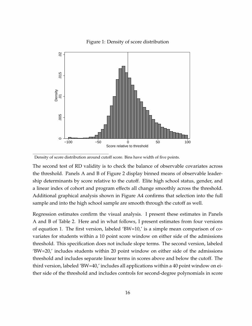
Figure 1: Density of score distribution

0.0

05.0

1.0

15.0

2D

ensi

ty

−100 −50 0 50 100Score relative to threshold

Density of score distribution around cutoff score. Bins have width of five points.

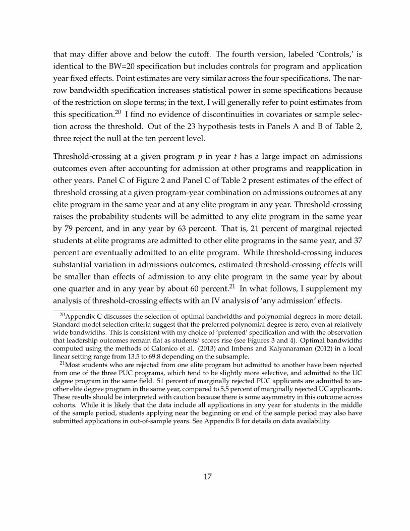
The second test of RD validity is to check the balance of observable covariates acrossthe threshold. Panels A and B of Figure 2 display binned means of observable leader-ship determinants by score relative to the cutoff. Elite high school status, gender, anda linear index of cohort and program effects all change smoothly across the threshold.Additional graphical analysis shown in Figure A4 confirms that selection into the fullsample and into the high school sample are smooth through the cutoff as well.

Regression estimates confirm the visual analysis. I present these estimates in PanelsA and B of Table 2. Here and in what follows, I present estimates from four versionsof equation 1. The first version, labeled ‘BW=10,’ is a simple mean comparison of co-variates for students within a 10 point score window on either side of the admissionsthreshold. This specification does not include slope terms. The second version, labeled‘BW=20,’ includes students within 20 point window on either side of the admissionsthreshold and includes separate linear terms in scores above and below the cutoff. Thethird version, labeled ‘BW=40,’ includes all applications within a 40 point window on ei-ther side of the threshold and includes controls for second-degree polynomials in score

16

that may differ above and below the cutoff. The fourth version, labeled ‘Controls,’ isidentical to the BW=20 specification but includes controls for program and applicationyear fixed effects. Point estimates are very similar across the four specifications. The nar-row bandwidth specification increases statistical power in some specifications becauseof the restriction on slope terms; in the text, I will generally refer to point estimates fromthis specification.20 I find no evidence of discontinuities in covariates or sample selec-tion across the threshold. Out of the 23 hypothesis tests in Panels A and B of Table 2,three reject the null at the ten percent level.

Threshold-crossing at a given program p in year t has a large impact on admissionsoutcomes even after accounting for admission at other programs and reapplication inother years. Panel C of Figure 2 and Panel C of Table 2 present estimates of the effect ofthreshold crossing at a given program-year combination on admissions outcomes at anyelite program in the same year and at any elite program in any year. Threshold-crossingraises the probability students will be admitted to any elite program in the same yearby 79 percent, and in any year by 63 percent. That is, 21 percent of marginal rejectedstudents at elite programs are admitted to other elite programs in the same year, and 37percent are eventually admitted to an elite program. While threshold-crossing inducessubstantial variation in admissions outcomes, estimated threshold-crossing effects willbe smaller than effects of admission to any elite program in the same year by aboutone quarter and in any year by about 60 percent.21 In what follows, I supplement myanalysis of threshold-crossing effects with an IV analysis of ‘any admission’ effects.

20Appendix C discusses the selection of optimal bandwidths and polynomial degrees in more detail.Standard model selection criteria suggest that the preferred polynomial degree is zero, even at relativelywide bandwidths. This is consistent with my choice of ‘preferred’ specification and with the observationthat leadership outcomes remain flat as students’ scores rise (see Figures 3 and 4). Optimal bandwidthscomputed using the methods of Calonico et al. (2013) and Imbens and Kalyanaraman (2012) in a locallinear setting range from 13.5 to 69.8 depending on the subsample.

21Most students who are rejected from one elite program but admitted to another have been rejectedfrom one of the three PUC programs, which tend to be slightly more selective, and admitted to the UCdegree program in the same field. 51 percent of marginally rejected PUC applicants are admitted to an-other elite degree program in the same year, compared to 5.5 percent of marginally rejected UC applicants.These results should be interpreted with caution because there is some asymmetry in this outcome acrosscohorts. While it is likely that the data include all applications in any year for students in the middleof the sample period, students applying near the beginning or end of the sample period may also havesubmitted applications in out-of-sample years. See Appendix B for details on data availability.

17

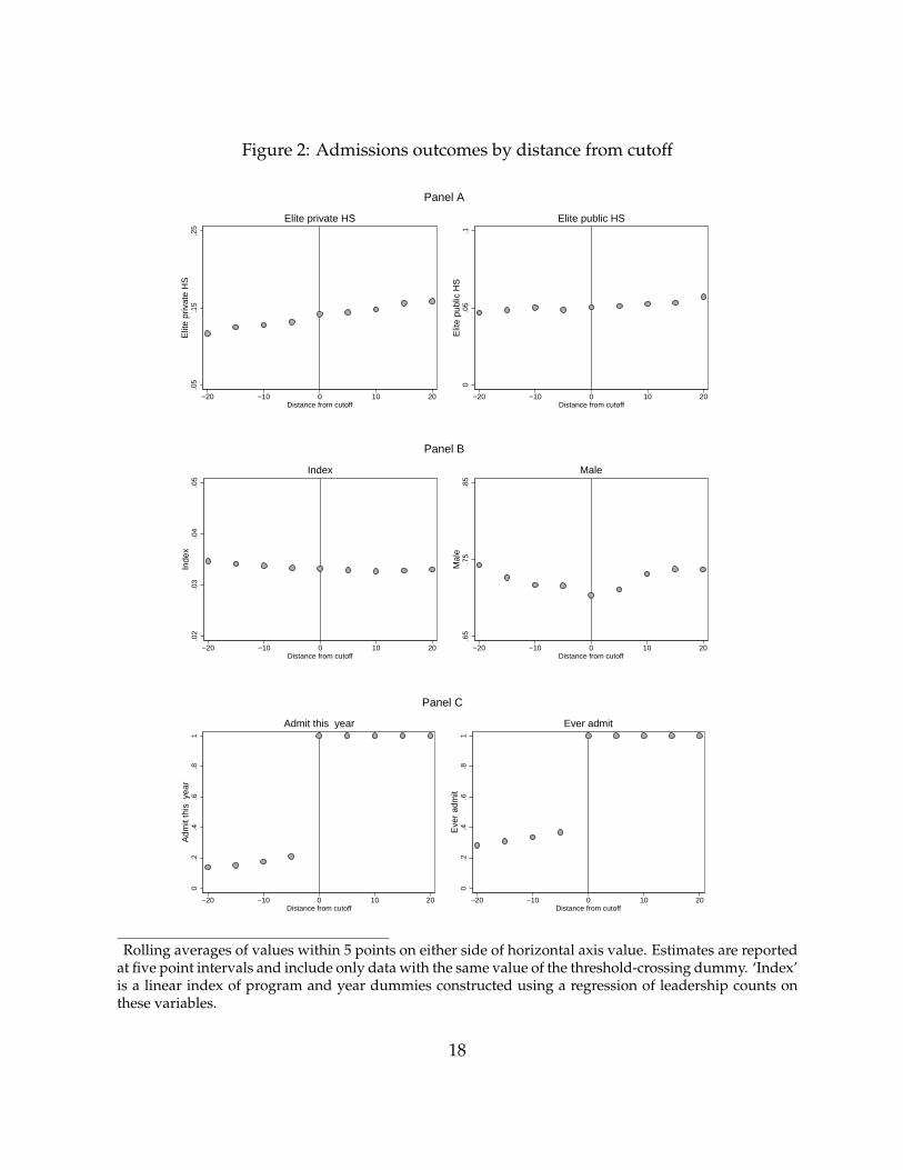
Figure 2: Admissions outcomes by distance from cutoff

.05

.15

.25

Elit

e pr

ivat

e H

S

−20 −10 0 10 20Distance from cutoff

Elite private HS

0.0

5.1

Elit

e pu

blic

HS


Elite public HS

Panel A.0

2.0

3.0

4.0

5In

dex


Index.6

5.7

5.8

5M

ale


Male

Panel B

0.2

.4.6

.81

Adm

it th

is y

ear


Admit this year

0.2

.4.6

.81

Eve

r ad

mit


Ever admit

Panel C

Rolling averages of values within 5 points on either side of horizontal axis value. Estimates are reportedat five point intervals and include only data with the same value of the threshold-crossing dummy. ‘Index’is a linear index of program and year dummies constructed using a regression of leadership counts onthese variables.

18

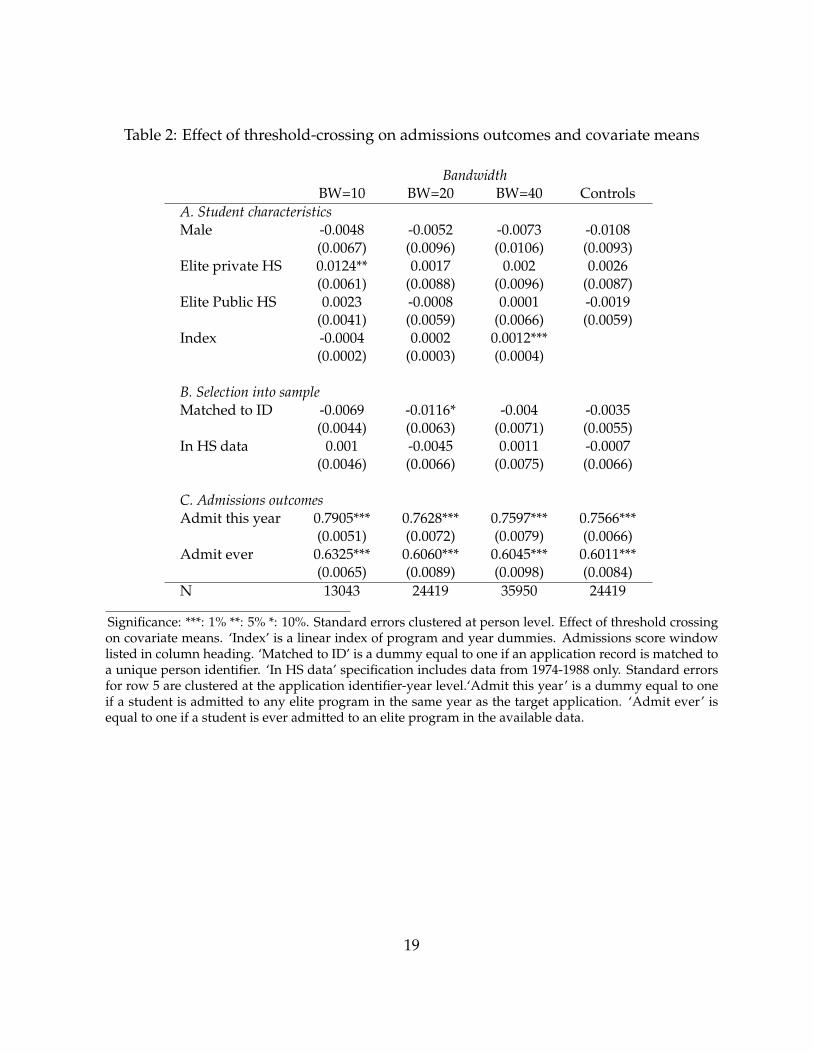
Table 2: Effect of threshold-crossing on admissions outcomes and covariate means

BandwidthBW=10 BW=20 BW=40 Controls

A. Student characteristicsMale -0.0048 -0.0052 -0.0073 -0.0108

(0.0067) (0.0096) (0.0106) (0.0093)Elite private HS 0.0124** 0.0017 0.002 0.0026

(0.0061) (0.0088) (0.0096) (0.0087)Elite Public HS 0.0023 -0.0008 0.0001 -0.0019

(0.0041) (0.0059) (0.0066) (0.0059)Index -0.0004 0.0002 0.0012***

(0.0002) (0.0003) (0.0004)

B. Selection into sampleMatched to ID -0.0069 -0.0116* -0.004 -0.0035

(0.0044) (0.0063) (0.0071) (0.0055)In HS data 0.001 -0.0045 0.0011 -0.0007

(0.0046) (0.0066) (0.0075) (0.0066)

C. Admissions outcomesAdmit this year 0.7905*** 0.7628*** 0.7597*** 0.7566***

(0.0051) (0.0072) (0.0079) (0.0066)Admit ever 0.6325*** 0.6060*** 0.6045*** 0.6011***

(0.0065) (0.0089) (0.0098) (0.0084)N 13043 24419 35950 24419

Significance: ***: 1% **: 5% *: 10%. Standard errors clustered at person level. Effect of threshold crossingon covariate means. ‘Index’ is a linear index of program and year dummies. Admissions score windowlisted in column heading. ‘Matched to ID’ is a dummy equal to one if an application record is matched toa unique person identifier. ‘In HS data’ specification includes data from 1974-1988 only. Standard errorsfor row 5 are clustered at the application identifier-year level.‘Admit this year’ is a dummy equal to oneif a student is admitted to any elite program in the same year as the target application. ‘Admit ever’ isequal to one if a student is ever admitted to an elite program in the available data.

19

4.2.2 Leadership outcomes

Figure 3: Leadership outcomes by distance from cutoff and firm type

.03

.05

.07

.09

N L

ead


N Lead

.02

.03

.04

.05

Any

lead


Any lead

.005

.015

.025

.035

List

ed o

n E

xcha

nge


Listed on Exchange

.02

.04

.06

Not

list

ed o

n E

xcha

nge


Not listed on Exchange

Rolling averages of values within 5 points on either side of horizontal axis value. Estimates are reportedat five point intervals and include only data with the same value of the threshold-crossing dummy. ‘Nlead’ counts total leadership positions. ‘Any lead’ is dummy equal to one if an individual is either adirector or an executive officer. ‘Listed on exchange’ and ‘Not listed’ count leadership positions at firmslisted and not listed on the Santiago Stock Exchange, respectively.

Figure 3 and Table 3 present estimates of the effect of admission on leadership outcomesfor all male applicants. The number of top management positions students hold risesby 50 percent across the admissions threshold, from 0.044 to 0.067. The probability thatstudents will hold any leadership position also rises by 50 percent, from 0.027 to 0.041.

20

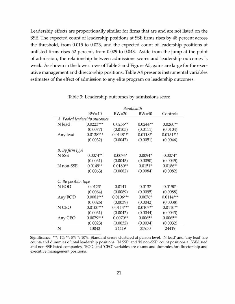
Leadership effects are proportionally similar for firms that are and are not listed on theSSE. The expected count of leadership positions at SSE firms rises by 48 percent acrossthe threshold, from 0.015 to 0.023, and the expected count of leadership positions atunlisted firms rises 52 percent, from 0.029 to 0.043. Aside from the jump at the pointof admission, the relationship between admissions scores and leadership outcomes isweak. As shown in the lower rows of Table 3 and Figure A5, gains are large for the exec-utive management and directorship positions. Table A4 presents instrumental variablesestimates of the effect of admission to any elite program on leadership outcomes.

Table 3: Leadership outcomes by admissions score

BandwidthBW=10 BW=20 BW=40 Controls

A. Pooled leadership outcomesN lead 0.0223*** 0.0256** 0.0244** 0.0260**

(0.0077) (0.0105) (0.0111) (0.0104)Any lead 0.0138*** 0.0148*** 0.0118** 0.0151***

(0.0032) (0.0047) (0.0051) (0.0046)

B. By firm typeN SSE 0.0074** 0.0076* 0.0094* 0.0074*

(0.0031) (0.0045) (0.0050) (0.0045)N non-SSE 0.0149** 0.0180** 0.0151* 0.0186**

(0.0063) (0.0082) (0.0084) (0.0082)

C. By position typeN BOD 0.0123* 0.0141 0.0137 0.0150*

(0.0064) (0.0089) (0.0095) (0.0088)Any BOD 0.0081*** 0.0106*** 0.0076* 0.0114***

(0.0026) (0.0039) (0.0042) (0.0038)N CEO 0.0100*** 0.0114*** 0.0107** 0.0110**

(0.0031) (0.0042) (0.0044) (0.0043)Any CEO 0.0079*** 0.0070** 0.0065* 0.0065**

(0.0023) (0.0032) (0.0034) (0.0032)N 13043 24419 35950 24419

Significance: ***: 1% **: 5% *: 10%. Standard errors clustered at person level. ‘N lead’ and ‘any lead’ arecounts and dummies of total leadership positions. ‘N SSE’ and ‘N non-SSE’ count positions at SSE-listedand non-SSE listed companies. ‘BOD’ and ‘CEO’ variables are counts and dummies for directorship andexecutive management positions.

21

The effects of college admission on leadership outcomes depend on high school back-ground. Figure 4 presents binned means of leadership outcomes for three groups ofstudents: those who attended elite private high schools, those who did not, and thesubset of the second group who attended elite public exam schools. Below thresholdstudents who attended elite private high schools hold an average of 0.117 executivemanagement and directorship positions, 335 percent more than the 0.035 average forstudents who did not attend elite high schools. For elite private high school students,the mean number of positions held jumps by 0.076 (65 percent) to 0.193 across the thresh-old, while the number of positions held by students from other high schools does notappear to jump at all. The result is a widening of the below-threshold gap in leadershipoutcomes. Above-threshold students hold 474 percent more top management positionsthan below-threshold students. Again, aside from the jump at the point of admission,there is a weak relationship between scores and leadership outcomes. Interestingly, re-sults for students who attended elite public exam schools are very similar to those forthe broader group of students who did not attend elite private high schools, if some-what noisier. As shown in the lower row of Figure 4, similar patterns hold for SSE andnon-SSE firms. Figure A6 presents results for directorship and executive managementpositions.

Table 4 reports regression results that bear out the visual analysis. The first columnpresents results for students who attended elite private high schools, the second col-umn presents results for students who did not, and the third presents results for thesubset of those students who attended elite public exam schools. The fourth columnpresents p-values from tests of equality of the elite private high school estimates and theestimates for all other students. The estimates shown here are from the BW=10 specifi-cation. Subsetting on the years for which high school data is available (1974-1988) andsplitting the sample by high school type substantially reduces precision relative to thepooled model. However, the effects of threshold-crossing on pooled and executive man-agement outcomes for students with private high school backgrounds remain significantat at least the ten percent level. Estimates for students who did not attend elite privatehigh schools are close to zero and statistically insignificant. Tests of equality betweenthe estimates for elite private high school students and other students reject at the tenpercent level for the most comprehensive leadership measure (total number of leader-ship positions held), as well as for total SSE-listed positions and executive management

22

positions.

Figure 4: Leadership outcomes by HS background and admissions score

0.0

5.1

.15

.2.2

5N

lead


Elite private Non−elite HS Exam

N lead

0.0

2.0

4.0

6.0

8.1

.12

.14

Any

lead



Any lead

0.0

2.0

4.0

6.0

8.1

List

ed o

n E

xcha

nge



Listed on Exchange

0.0

5.1

.15

Not

list

ed o

n E

xcha

nge



Not listed on Exchange

Rolling averages of values within 5 points on either side of horizontal axis value. Estimates are reportedat five point intervals and include only data with the same value of the threshold-crossing dummy. ‘Non-elite HS’ pools data for all schools that are not elite private high schools. The ‘exam’ category is thesubset of applications from the non-elite HS group from public exam schools. ‘Listed on exchange’ and‘Not llisted’ count leadership positions at firms listed and not listed on the Santiago Stock Exchange,respectively.

Table A5 presents instrumental variables estimates of the effects of ever being admittedto an elite degree program on leadership outcomes. For students from elite private highschools, the gain in leadership positions associated with any admission is 0.141, whilefor other students it is 0.009. I highlight these results here because I will use them in the

23

decomposition exercise in Section 6. Table A6 presents equivalent results for the BW=20and BW=40 specifications. Point estimates from these specifications are similar to thosepresented in Table 4. However, the inclusion of above- and below-threshold polynomialterms reduces precision. For instance, the estimated effect of threshold-crossing on thecount of leadership outcomes for elite high school students is 0.0881 with a standarderror of 0.0576, compared to a point estimate of 0.0760 with a standard error 0.0365 inthe BW=10 specification.

Table 4: Effects of admission on leadership outcomes by high school type

I. Elite private II. Not elite private III. Public exam Test: I v. IIA. Pooled leadership outcomesN lead 0.0760** 0.0058 0.0147 0.0611*

(0.0365) (0.0088) (0.0208)Any lead 0.0295** 0.0055 0.0026 0.1139

(0.0146) (0.0038) (0.0114)

B. By firm typeN SSE 0.0318* -0.0012 -0.0091 0.0615*

(0.0177) (0.0030) (0.0104)N non-SSE 0.0442* 0.0074 0.0238 0.1586

(0.0250) (0.0074) (0.0181)

C. By position typeN BOD 0.0495 0.0019 0.001 0.1545

(0.0326) (0.0076) (0.0073)Any BOD 0.0149 0.0023 0.001 0.3122

(0.0121) (0.0030) (0.0073)N CEO 0.0266** 0.0039 0.0137 0.0577*

(0.0114) (0.0036) (0.0190)Any CEO 0.0238** 0.0041 -0.0018 0.0789*

(0.0109) (0.0027) (0.0095)N 1513 6965 562

Significance: ***: 1% **: 5% *: 10%. Standard errors clustered at person level. Estimates of admissionseffects from BW=10 specification. ‘Non-elite HS’ pools data for all schools that are not elite private highschools. The ‘public exam’ category is the subset of applications from the column II for students frompublic exam schools. p-value column reports tests of equality of coefficients for students from elite privatehigh schools and other students.

24

5 Peer ties in management hiring

The results above show that elite university admission plays a causal role in the pro-duction of top managers, but only for students who attended elite private high schools.Broadly speaking, there are two ways to explain this finding. The first is complemen-tarity between an elite private high school background and institutional inputs such ascoursework, faculty interaction, or ‘sheepskin’ signaling effects. For example, reachinga top management position could require both the skills learned at elite colleges andfluency in English. Students attending elite private high schools are often taught En-glish at a young age, while other students are not and may be unable to catch up. Itcould also be the case that admission to an elite college provides a stronger signal aboutthe management productivity of elite high school students than about students who at-tended other high schools. What these types of effects have in common is that they donot depend upon interactions between college students. The second explanation is thatit is precisely these interactions that are important. For example, students who attendedelite private high schools might have ties to businesses through which they can refercollege peers. Alternatively, school peers may be more productive if they work together,and working with peers may incentivize good management behavior. Students fromelite high school backgrounds could benefit disproportionately if they are better able toform these kinds of ties with other students from elite backgrounds. This section askshow much of the observed effect of admission to elite degree programs can be attributedto peer ties.

I study peer ties by looking at co-leadership rates, which I define as the expected numberof firms where both members of a pair of students have leadership positions. I compareco-leadership rates for students who were college peers (i.e., who attended the same de-gree program at the same time) to co-leadership rates for pairs who attended the samedegree program at different times, or who attended a different degree program at thesame time. The intuition is that within a degree program, same-year pairs are similar topairs of students a few years apart in terms of pre-college backgrounds and institutionalinputs, but that students in same-year pairs are more likely to know each other and tohave mutual contacts. If students obtain jobs through contacts, or if peers are more pro-ductive when working together, college peers may be more likely to serve on leadershipteams at the same firms than other pairs of similar students. If management hiring de-

25

pends only on non-peer institutional inputs, there would be little reason to expect sucha result.

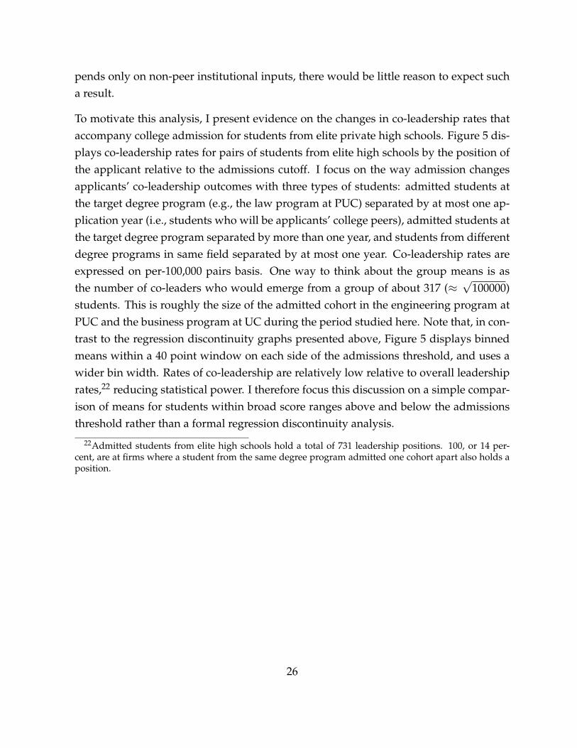
To motivate this analysis, I present evidence on the changes in co-leadership rates thataccompany college admission for students from elite private high schools. Figure 5 dis-plays co-leadership rates for pairs of students from elite high schools by the position ofthe applicant relative to the admissions cutoff. I focus on the way admission changesapplicants’ co-leadership outcomes with three types of students: admitted students atthe target degree program (e.g., the law program at PUC) separated by at most one ap-plication year (i.e., students who will be applicants’ college peers), admitted students atthe target degree program separated by more than one year, and students from differentdegree programs in same field separated by at most one year. Co-leadership rates areexpressed on per-100,000 pairs basis. One way to think about the group means is asthe number of co-leaders who would emerge from a group of about 317 (≈

√100000)

students. This is roughly the size of the admitted cohort in the engineering program atPUC and the business program at UC during the period studied here. Note that, in con-trast to the regression discontinuity graphs presented above, Figure 5 displays binnedmeans within a 40 point window on each side of the admissions threshold, and uses awider bin width. Rates of co-leadership are relatively low relative to overall leadershiprates,22 reducing statistical power. I therefore focus this discussion on a simple compar-ison of means for students within broad score ranges above and below the admissionsthreshold rather than a formal regression discontinuity analysis.

22Admitted students from elite high schools hold a total of 731 leadership positions. 100, or 14 per-cent, are at firms where a student from the same degree program admitted one cohort apart also holds aposition.

26

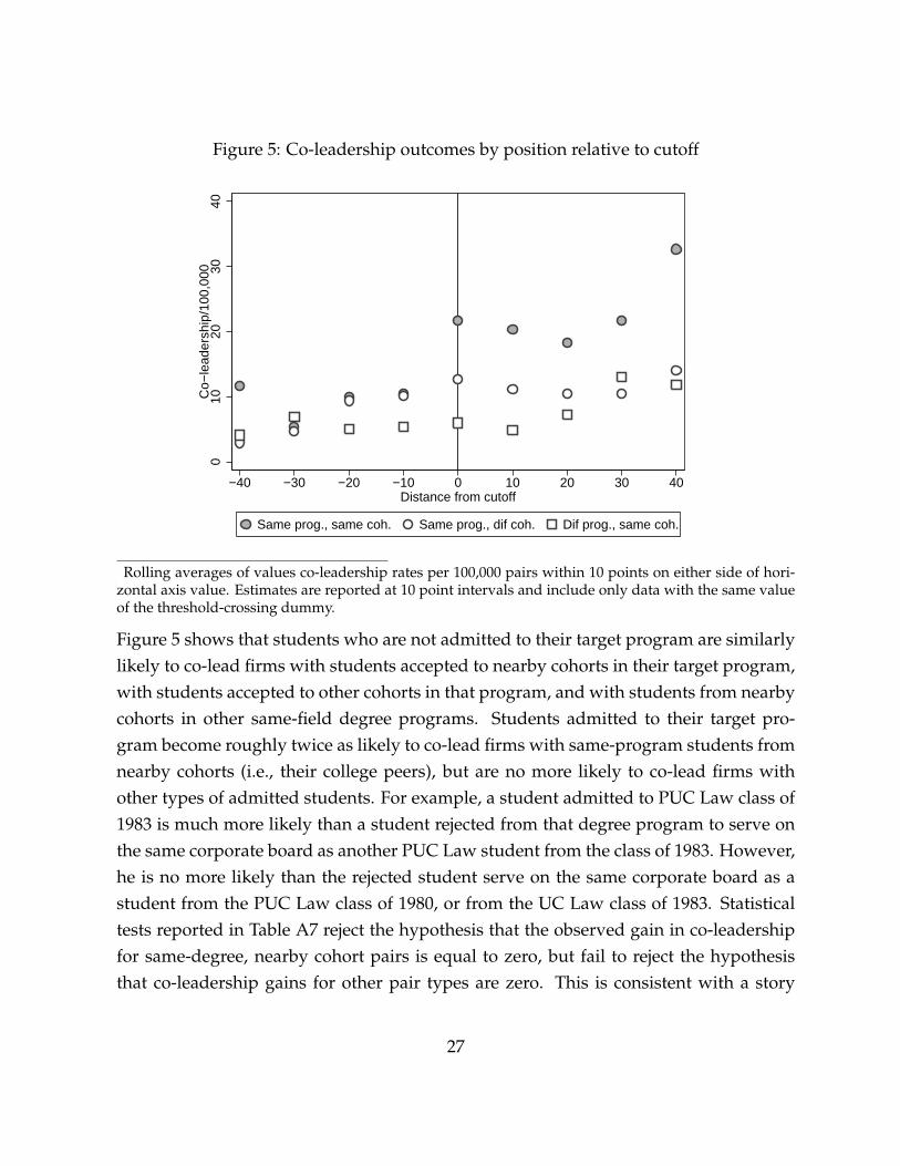
Figure 5: Co-leadership outcomes by position relative to cutoff

010

2030

40C

o−le

ader

ship

/100

,000

−40 −30 −20 −10 0 10 20 30 40Distance from cutoff

Same prog., same coh. Same prog., dif coh. Dif prog., same coh.

Rolling averages of values co-leadership rates per 100,000 pairs within 10 points on either side of hori-zontal axis value. Estimates are reported at 10 point intervals and include only data with the same valueof the threshold-crossing dummy.

Figure 5 shows that students who are not admitted to their target program are similarlylikely to co-lead firms with students accepted to nearby cohorts in their target program,with students accepted to other cohorts in that program, and with students from nearbycohorts in other same-field degree programs. Students admitted to their target pro-gram become roughly twice as likely to co-lead firms with same-program students fromnearby cohorts (i.e., their college peers), but are no more likely to co-lead firms withother types of admitted students. For example, a student admitted to PUC Law class of1983 is much more likely than a student rejected from that degree program to serve onthe same corporate board as another PUC Law student from the class of 1983. However,he is no more likely than the rejected student serve on the same corporate board as astudent from the PUC Law class of 1980, or from the UC Law class of 1983. Statisticaltests reported in Table A7 reject the hypothesis that the observed gain in co-leadershipfor same-degree, nearby cohort pairs is equal to zero, but fail to reject the hypothesisthat co-leadership gains for other pair types are zero. This is consistent with a story

27

in which ties to college peers account for an important component of the overall gainsfrom admission, but difficult to reconcile with a story based on peer-independent skills.In the next subsection, I formalize this intuition using a model of top management hir-ing.

5.1 Model of top management hiring

I present a simple model of top management hiring in which hiring depends on stu-dent skills and referrals from school peers. This exercise has two goals. The first is toshow how an analysis of changes in co-leadership rates across the admissions thresh-old such as that presented above can provide insight into the relative importance ofthe peer effects channel. The second is to develop a formula relating differences in co-leadership rates for pairs of students who are and are not college peers to the overallgain in leadership positions associated with admission. This will provide the basis fora decomposition of the total effect of admission into a ‘skill’ component and a ‘peers’component.

In the model, peer ties help students by providing firms with information about studentproductivity. As mentioned above, peer ties could also operate through other channels.I return to this point in section 6. I design the model to capture three intuitive featuresof top management hiring decisions. First, admission to an elite degree program mayhelp students develop skills applicable at many firms, and may also connect studentsto peers who make top management hiring decisions at specific firms. Second, becausea very small number of students advance in a firm to the point where they are able todecide which top managers to hire, students from different degree programs may haveconnections to different firms even if each degree program is quite large. Third, evenwithin degree programs, access to connections may depend on students’ friend groups,which in turn may depend on social class.

To ensure the model is tractable, I consider a very simple framework for hiring decisionsand the formation of peer connections.23 Model setup is as follows. Students may attend

23Strong restrictions on the hiring process and the form of peer connections (or complementarities) areoften necessary to obtain tractable solutions in agglomeration models. The closest parallel in the existingliterature is Oyer and Schaefer (2012), who adopt the model of Ellison and Glaeser (1997). This analysisdiffers from Oyer and Schaefer in that my goal is to relate extensive-margin changes in hiring outcomes

28

either elite or non-elite high schools, indexed by d ∈ {l, h}. They may attend either eliteor non-elite college degree programs; there are P elite degree programs, each with ameasure of students. There are F total firms hiring top managers. Hiring is independentacross firms, and students may hold positions at multiple firms. The latter point isconsistent with the observed data.

Hiring depends on students’ skills and on referrals from college peers. Students take oneof two skill types: productive or unproductive. I use the term ‘productivity’ loosely; itmay reflect firm profitability, but could also reflect the incentives of those making thehiring decision. The probability a student is the productive type depends on what kindof high school and college he attended. A student who attended a type d high schooland a non-elite college is productive with probability γd. If that student attends an elitecollege, the probability he is productive rises to γd + bd. The model captures skill com-plementarities by permitting bh to be larger than bl; i.e., skill gains can be larger for stu-dents from elite high schools. Skill endowments are independent across students.

Firm incentives are such that a firm hires a worker if and only if the firm knows theworker is productive. Fraction π of firms observe students’ skill types and do not facean informational constraint. Fraction (1− π) do not observe skill types. These firms re-ceive information on skills from referrals. Referrals, which reveal student productivitywithout error, are available only from same-type college peers with ex-ante connectionsto particular firms. For simplicity, I assume that there is precisely one student per firmwho can provide referrals, and that referral-providing students always attend elite de-gree programs. The former assumption can be relaxed; the key feature is that referralscannot be so common that they are available at all elite degree programs. I discuss theempirical basis for the latter restriction below. One could think of the students provid-ing referrals as having family connections to firms, or as advisers to hiring committeeschosen prior to management hiring. The probability that the referral-providing studentfor firm f is of high school type d and attends elite degree program p is rd. Such studentsprovide referrals to all of their same-type college peers.

The network setup described here captures in a simple way the idea that connectionsto firms are more common in elite degree programs and vary across both elite degreeprograms and social groups. I now consider the effects of elite college admission on

to gains from peer ties, whereas Oyer and Schaefer conduct their analysis within a sample of individualsalready employed at law firms.

29

hiring outcomes. Let Yidp f be a dummy variable equal to one if student i from highschool d attending elite college degree program p is hired for a top management roleat f , and let Yid0 f be a dummy variable equal to one if i from high school d attendinga non-elite college degree program is hired at f . Then we may write the effect of eliteadmission on expected total leadership positions for students from high school type das

E

[∑

f(Yidp f −Yid0 f )|d

]= F× (bdπ + rd(γd + bd)(1− π))

or∆d = Sd + Cd (2)

where ∆d = E[∑ f (Yidp f −Yid0 f )|d

], Sd = F× (bdπ), and Cd = F× (rd(γd + bd)(1− π)).

The total gain in leadership positions is equal to the sum of skill component Sd, whichis equal to zero if skill gain bd is zero, and connections component Cd, which is equal tozero if connections gain rd is zero. The evidence in section 4 suggests that either Sh > Sl,Ch > Cl, or both.

Co-leadership outcomes can provide insight into the relative importance of Sd and Cd

in ∆d. I focus on two model implications. The first model implication is that, for stu-dents gaining admission to elite degree program p who would otherwise have attendeda non-elite college, a) any increase in the rate of co-leadership with students at someother elite degree program q is due to skill gains, and b) any additional increase in therate of co-leadership with college peers at p is attributable to network effects. More for-mally, let κ

di fd be the change in rates of co-leadership with non-peers associated with elite

admission, and let κsamed be the change in rates of co-leadership with peers. For example,

consider an experiment in which a student is randomly assigned admission to PUC Lawrather than admission to some non-elite degree program. κ

di fd reflects the expected gain

in co-leaders from some other elite degree program (e.g., UC Law), while κsamed reflects

the expected gain in co-leaders also from PUC Law.

Then, for a pair of students i 6= j, and two elite degree programs p 6= q, we maywrite

30

κdi fd = E

[∑

f

(Yidp f Yjdq f −Yid0 f Yjdq f

)|d]

= F(γd + bd)bdπ (3)

and

κsamed = E

[∑

f

(Yidp f Yjdp f −Yid0 f Yjdp f

)|d]

= κdi fd + rdF(γd + bd)

2(1− π) (4)

The admissions gain in co-leadership rates with non-peers, κdi fd , is equal to zero if skill

gains bd are equal to zero, or if π = 0 and there are no firms that observe skill gainswithout referrals. The admissions gain in co-leadership with peers, κsame

d , is equal to κdi fd

plus a term that is greater than zero only if network gains rd are greater than zero and ifsome firms do not observe skill perfectly.

The second model implication is that the connection effect term Cd can be expressedas the difference in co-leadership rates for pairs of college peers relative to non-peersmultiplied by a scaling term. Specifically,

Cd = τd ×E[∑ f Yidp f |d]

E[∑ f Yidp f Yjdp f |d](5)

where τd = E[∑ f(Yidp f Yjdp f −Yidp f Yjdq f

)|d]. The scaling term, which is equal to

(γd + bd)−1, accounts for the fact that students can only form co-leadership pairs if both

members are the productive type.

This model abstracts from potentially important forms of heterogeneity by assumingthat degree programs and firms are homogeneous. It is possible that students admittedto different degree programs or fields of study have skill sets that match particularlywell to certain firms. It could also be the case that students from particular cohorts

31

are more valuable to some firms if career paths for students of a certain age coincidewith a firm’s management hiring schedule. I address these concerns in my empiricalwork using first difference and difference-in-differences approaches that compare pairsof students in the same degree programs but different cohorts and different degree pro-grams in the same field and the same cohort. Appendix D extends the model to the casein which productivity at specific firms varies across degree programs and cohorts, anddescribes conditions under which difference-in-difference approaches account for thisheterogeneity. As is standard in difference-in-difference analyses, the key assumptionis that firm-program-type effects and firm-cohort-type effects are additively separable;i.e., that there are not differential changes in the skill match between degree programsand firms over time.

5.2 Estimating gains from peer connections

The first model implication maps fairly straightforwardly to results presented above inFigure 5. The model indicates that, if elite admission increases rates of co-leadershipwith students who are not peers at the targeted elite degree program, this can be inter-preted as evidence of skill gains. If co-leadership gains with peers at the elite degreeprogram targeted for admission exceed co-leadership gains with non-peers, this is evi-dence of gains from peer connections. Figure 5 shows that admission to an elite degreeprogram only increases co-leadership rates with college peers at that degree program,not with students who attend that program in different years or who attend differentprograms in the same field. This suggests a limited role for skill effects in driving over-all gains from admission, and a potentially large role for peer effects.24

The second model implication is that the connection effect component of total admis-sions gains, Cd, can be expressed as the difference in co-leadership rates for pairs ofcollege peers relative to non-peers, τd, multiplied by a scaling term. I estimate differ-ences in co-leadership rates for elite college peers and non-peers using single-differenceand difference-in-difference specifications of the form

24One complication in mapping the model to the regression discontinuity analysis is that threshold-crossing into admission at one degree program is associated with a reduced probability of attending thesame-field program in the other institution (see Table 2 and the associated discussion). If peer effects mat-ter, this could drive up the gains in co-leadership outcomes with college peers relative to other students.I discuss the value of peer ties for rejected students in more detail below.

32

Y jd′pt′

idpt = β0 + β1C(t, t′) + ejd′pt′

idpt (6)

and

Y jd′p′t′

idpt = π0 + π1C(t, t′) + π2S(p, p′) + π3C(t, t′)S(p, p′) + ejd′p′t′

idpt . (7)

Here, Y jd′pt′

idpt counts the total number firms where applicants ipt and jp′t′ both hold po-sitions. C(t, t′) is an indicator variable equal to one if |t − t′| ≤ 1; i.e., if two studentsin question attended school within one cohort of one another. S(p, p′) is an indicatorvariable equal to one if p = p′, i.e., if both students in the pair are at the same degreeprogram. I label students college peers if C(t, t′) and S(p, p′) both equal one. I estimateequation 6 using only pairs of admitted applications to the same degree program (e.g.,PUC law-PUC law pairs). I estimate equation 7 using pairs of admitted applications tothe same field (e.g., PUC law-PUC law pairs and PUC law-UC law pairs). I estimateboth equations separately for pairs of students from elite high schools, pairs of studentsfrom non-elite high schools, and mixed pairs. My model stipulates that referrals shouldact only through pairs of students from the same type of high school; the inclusion ofmixed pairs can be viewed as test of this restriction.

Panel A of Table 5 presents estimates of equation 6. The three left columns display esti-mates where the sample is restricted to pairs from application cohorts five or fewer yearsapart, while the right three columns display estimates for pairs at any cohort distance.Columns display estimates of equation 6 for elite-elite, elite-non-elite and non-elite-non-elite pairs, respectively. I compute standard errors that allow for clustering of the er-ror term separately by i and j; i.e., clustering at the student by student level (Cameronet al. 2011). Appendix E discusses approaches to clustering in pairwise datasets andpresents results obtained using alternate clustering strategies.

Within all same-degree pairs where students are at most five cohorts apart, pairs of elitehigh school students who attended the same college but not at the same time becomeco-leaders of firms at a rate of 13.9 per 100,000. For students who are college peers,this rate rises by 13.0, or 93 percent, to 26.9 per 100,000. This change is statisticallysignificant at the one percent level. For pairs in which one student attended an elite

33

high school and one did not, the baseline co-leadership rate is 2.5, and this rate risesby a statistically insignificant 0.6 (24 percent) for college peers. For pairs of non-elitestudents, the baseline co-leadership rate is 0.7 per 100,000, and this rises by 0.3, or 44percent, for college peers. This change is statistically significant at the ten percent level.These results are stable when the sample is expanded to include all same-degree pairs,not just those within five years of one another, with the exception that the effect for pairsof non-elite students becomes statistically insignificant.That results are insensitive to thischange in sample indicates that patterns of management recruitment are relatively stablewithin institutions over time.25

25This suggests that my results are not driven by life-cycle patterns in top management attainment. Italso argues against a corporate recruitment story. If certain firms only recruit at certain degree programsin a subset of years, this could potentially lead to results like those observed here. Concerns about theeffects of differential corporate recruitment across degree programs and cohorts are surely lower here,where the outcomes in question are realized roughly 30 years after graduation, than they would be forentry level positions. They are also mitigated by the fact that all of the programs here are located inSantiago, reducing costs associated with separate recruitment visits. In any case, if corporate recruitingdid differ within programs across years, one might expect higher rates of co-leadership for students incloser cohorts who face more similar recruiting environments. Comparing panels A and B suggests thatthis is not the case.

34

Table 5: Mean co-leadership rates for student pairs, by type of pair

I. Within 5 years II. All pairsElite- Elite- Not elite- Elite- Elite- Not elite-

A. Within same degree elite not elite not elite elite not elite not eliteClose cohort 13.0*** 0.6 0.3* 12.9*** 1 0.4

(4.4) (0.6) (0.2) (5.0) (0.6) (0.2)Constant 13.9*** 2.5*** 0.7*** 13.9*** 2.2*** 0.6***

(3.4) (0.5) (0.1) (2.9) (0.5) (0.1)N 740928 7086379 21539977 1115903 11123695 34730816

B. Within same fieldSame degree × close cohort 16.5*** 0.7 0.4 16.6*** 1.3* 0.5

(5.3) (0.7) (0.3) (5.2) (0.8) (0.3)Same degree 2.8 -0.2 -0.1 2.7 -0.8* -0.2

(2.4) (0.4) (0.1) (2.8) (0.4) (0.1)Close cohort 3.5 -0.1 -0.1 3.7 -0.4 -0.1

(2.9) (0.4) (0.2) (2.8) (0.3) (0.2)Constant 11.0*** 2.76*** 0.7*** 11.2*** 2.9*** 0.8***

(2.4) (0.5) (0.1) (2.3) (0.4) (0.1)N 1478180 13719925 32949927 2215586 21304466 52514174

Significance: ***: 1% **: 5% *: 10%. Units are co-leadership rates per 100,000 pairs. Standard errors usetwo-way clustering at student by student level. ‘Elite-elite’ columns subset on pairs of admitted studentsin which both students attended an elite private high school. ‘Elite-not elite’ subsets on pairs where onestudent attended an elite private high school and one did not. ‘Not elite-not elite’ pairs are those for whichneither student attended an elite private high school.

35

Panel B of Table 6 presents estimates of equation 7. These estimates follow a similarpattern to estimates from Panel A, but point estimates on peer effect terms are gener-ally larger. Pairs of elite high school students from the same field and non-close cohortsbecome co-leaders at rate of 11.0 per 100,000. This rises by 3.5 per 100,000 for studentsfrom nearby cohorts, and by 2.8 per 100,000 for students in the same institution. Nei-ther of these effects is statistically significant. For students in the same institution andnearby cohorts, co-leadership rates rise by 16.5 per 100,000. This effect is significant atthe one percent level, and is stable when the sample is expanded to include all cohortdistances. As was the case for equation 6, estimates of peer effects for pairs of elite andnon-elite students and pairs of non-elite students are substantially smaller in both levelsand percentage terms, and are generally not statistically significant.

These estimates of τd are consistent with a large role for peer ties in the overall admis-sions effect. Table 6 presents a decomposition of total admissions effects for studentsfrom elite private high schools and students from other high schools. The first columnrepeats differences and difference-in-differences estimates of τd from Table 5. The sec-ond column is the scaling factor from equation 5, divided by 100,000 to account for theunits in the τd term. The scaling factor is just the ratio of leadership rates to co-leadershiprates amongst college peers of a given type. Column three presents the estimated peer tieterm Cd obtained by multiplying columns one and two. The single differences estimatessuggest that peer ties increase the number of leadership positions held by students fromelite private high schools by 0.11, compared to 0.02 for other students. Difference-in-differences estimates suggest peer-related gains of 0.14 for private high school students,and 0.02 for other students. Peer ties account for 80 to 100 percent of the overall admis-sions effect for elite private high school students.

36

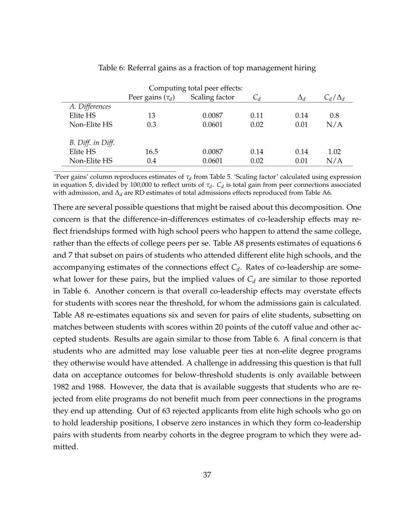
Table 6: Referral gains as a fraction of top management hiring

Computing total peer effects:Peer gains (τd) Scaling factor Cd ∆d Cd/∆d

A. DifferencesElite HS 13 0.0087 0.11 0.14 0.8Non-Elite HS 0.3 0.0601 0.02 0.01 N/A

B. Diff. in Diff.Elite HS 16.5 0.0087 0.14 0.14 1.02Non-Elite HS 0.4 0.0601 0.02 0.01 N/A

‘Peer gains’ column reproduces estimates of τd from Table 5. ‘Scaling factor’ calculated using expressionin equation 5, divided by 100,000 to reflect units of τd. Cd is total gain from peer connections associatedwith admission, and ∆d are RD estimates of total admissions effects reproduced from Table A6.

There are several possible questions that might be raised about this decomposition. Oneconcern is that the difference-in-differences estimates of co-leadership effects may re-flect friendships formed with high school peers who happen to attend the same college,rather than the effects of college peers per se. Table A8 presents estimates of equations 6and 7 that subset on pairs of students who attended different elite high schools, and theaccompanying estimates of the connections effect Cd. Rates of co-leadership are some-what lower for these pairs, but the implied values of Cd are similar to those reportedin Table 6. Another concern is that overall co-leadership effects may overstate effectsfor students with scores near the threshold, for whom the admissions gain is calculated.Table A8 re-estimates equations six and seven for pairs of elite students, subsetting onmatches between students with scores within 20 points of the cutoff value and other ac-cepted students. Results are again similar to those from Table 6. A final concern is thatstudents who are admitted may lose valuable peer ties at non-elite degree programsthey otherwise would have attended. A challenge in addressing this question is that fulldata on acceptance outcomes for below-threshold students is only available between1982 and 1988. However, the data that is available suggests that students who are re-jected from elite programs do not benefit much from peer connections in the programsthey end up attending. Out of 63 rejected applicants from elite high schools who go onto hold leadership positions, I observe zero instances in which they form co-leadershippairs with students from nearby cohorts in the degree program to which they were ad-mitted.

37

6 Discussion

This paper considers the role of elite colleges in providing a pathway for talented stu-dents from non-elite backgrounds into top management roles at major corporations. Toaddress this question, I combine rich and novel data on applicants to elite business, law,and engineering programs in Chile between 1968 and 1995 with a regression discontinu-ity design that exploits score-based admissions cutoffs. I find that admission to an elitedegree program raises the number of leadership positions students hold by 50 percent,but that these gains accrue only to students who attended elite private high schools.Students who attend other types of high schools, including elite public schools, do notrealize any gains in leadership outcomes from elite college admission.

The composition of leadership teams at particular firms suggests that ties formed be-tween college peers from elite private high schools are an important driver of top man-agement hiring. Pairs of private school students who attend the same degree programsat similar times are 93 percent more likely to serve on leadership teams at the samefirm than pairs of private school students who attend the same degree program in moredistant years, and 133 percent more likely than pairs of private high school studentswho attend different programs in the same field at similar times. Students who are notfrom private high schools are not significantly more likely to co-lead firms with col-lege peers who attended private high schools than they are with students from differentdegree programs or different cohorts. A simple model of referral based hiring relatesthese findings to overall admissions effects, and allows for a decomposition of total ad-missions effects into a ‘peers’ component and an ’other inputs’ component. The modelindicates that peer ties are the key driver of overall admissions effects. Specifically, peerties account for 80 to 100 percent of the hiring gain for students from elite private highschools.

One surprising aspect of these findings is that, even in the presence of a transparent ad-missions system (based only on test scores and grades, and notably without the legacypreferences common in the US), elite colleges appear to widen the leadership gap be-tween students from elite private high schools and students from other high schools,including elite public exam schools. This is an important observation, because highereducation is perhaps the main avenue open to policymakers hoping to connect talentedstudents from non-elite backgrounds with high-end skill inputs and connections to elite-

38

background peers. In Chile, as in the United States, elite private high schools cost farmore than available subsidies and frequently have opaque admissions criteria (Nielson2013). In contrast, loans and scholarships are more readily available to cover collegecosts, and the admissions process is relatively transparent.26 Elite colleges in both Chileand the US appear to be aware of the unique role they play in identifying and devel-oping talented students from non-elite backgrounds.27 However, my findings suggestthat these efforts have not been fully successful, perhaps because students from eliteand non-elite backgrounds tend to self-segregate. Understanding the effects of effortsaimed at increasing within-school integration on leadership outcomes should be a highresearch priority.

My findings are consistent with two stories in which the dominance of a small groupof elites reduces social welfare. The failure of elite universities to facilitate innovationamongst the economic elite could be a driver or a symptom (or both) of the type ofgrowth-reducing elite entrenchment described, e.g., in Acemoglu and Robinson (2006,2008, 2012). Even abstracting from possible growth effects, the absence of an elite edu-cation pathway to top management positions for students from non-elite backgroundsmay have deleterious welfare effects. Authors dating back to Marx (1865) and de Toc-queville (1830-35) have argued that low social position is more tolerable when advance-ment seems plausible (see Ferrie 2005 for a discussion). The magnitude of welfare lossesthrough these two channels is of course very difficult to quantify.

My results have more ambiguous implications for the efficiency of corporate manage-ment. A growing literature suggests that managers’ skills and backgrounds can affectfirm performance (Bertrand and Schoar 2003; Malmendier and Tate 2005, 2010; Guner etal. 2008; Lazear et al. 2012). This means that welfare losses could accrue if talented butunconnected individuals cannot reach the executive suite. The model of informationalfrictions in hiring that I develop in this paper is consistent with this story. Welfare im-plications are less clear, however, if peer ties can affect managerial productivity directly.Recent papers suggest that peer connections among managers could either reduce effi-

26Though Hoxby and Turner (2013) and Dynarski and Scott-Clayton (2008) do raise questions about thetransparency of the college admissions and financial applications in the U.S., particularly for low-incomeapplicants.

27For instance, the business program at the University of Chile lists as part of its mission statement ‘pre-serv[ing] a diverse student body’ and ‘recruit[ing] and retain[ing] high potential undergraduate students’(Agosin 2012). Part of Harvard’s stated mission is to ‘identify and remove constraints on students’ fullparticipation, so that individuals may... develop their full intellectual and human potential’ (Lewis 1997).

39

ciency by encouraging lax oversight or inefficient compensation decisions (Fracassi andTate 2012; Shue 2013), or increase efficiency by facilitating the flow of information withinand across firms or by taking advantage of peer complementarities in production (Co-hen et al. 2008; Oyer and Schaefer 2012). Network inputs into manager performancecould mitigate or eliminate welfare losses due to informational frictions in hiring; alter-natively, they could exacerbate these losses. This is a topic for future research.

Another important question is whether results from Chile can be meaningfully extrap-olated to other countries. It seems likely that access to elite educational institutions andfamily networks play a smaller role in Chile than in other Latin American countries,which are characterized by slower growth, similar levels of inequality, and less businesstransparency. Comparisons with the US and European countries are more challeng-ing. Lower levels of GDP and higher inequality suggest that access to elite educationaland family networks may play a larger role in Chile in the population as a whole. Thepresent analysis, however, focuses on applicants to elite colleges, a privileged group.Cross-country comparisons of inequality are not as straightforward after conditioningon college application. The fraction of students attending college in Chile during theperiod in question was far smaller than the fraction in the US, which suggests thatcross-country differences in inequality could be reduced or even reversed within thesubpopulation of applicants.

Further complicating the comparison are differences in the size and geographic disper-sion of the business elite. Chile has a relatively small corporate sector concentrated inone city, Santiago. The US has a much larger set of business leaders distributed acrossseveral major population centers. On the one hand, this suggests that, at the nationallevel, peer ties between corporate leaders may be stronger in Chile. On the other hand,elite university attendance in the US could be even more valuable if opportunities to net-work with a nationally-recruited group of elite students are rarer. The direction of ‘bias’in Chilean estimates of overall admissions effects and heterogeneous admissions effectsby family background relative to population parameters in the US is unclear.

I conclude with an important caveat: My results do not indicate that students from non-elite high schools get no benefits from elite admission. HNZ (2013) show that studentsfrom lower tier high schools do realize earnings gains from admission to selective degreeprograms. Further, it is possible that some students from non-elite high schools become

40

leaders in other fields, such as politics. Questions about when students from non-elitehigh schools leave the corporate leadership track and whether they attain leadershiproles in other fields are important, and represent a pathway for future work using early-career data and data on leadership outcomes outside of the private sector. A findingthat students from non-elite high schools become leaders in areas other than businesswould arguably make the finding that they do not reach top management positions inthe corporate world more surprising.

References

Acemoglu, Daron and James A. Robinson, “Political losers as a barrier to economicdevelopment,” The American Economic Review, 2000, 90 (2), 126–130.

and , “Economic backwardness in political perspective,” American PoliticalScience Review, 2006, 100 (1), 115–131.

and , “Persistence of Power, Elites, and Institutions,” The American EconomicReview, 2008, 98 (1), 267–93.

and , Why nations fail: The origins of power, prosperity, and poverty, RandomHouse Digital, Inc., 2012.

, Simon Johnson, and James A. Robinson, “The Colonial Origins of ComparativeDevelopment: An Empirical Investigation,” The American Economic Review, 2001.

Agosin, Manuel, “Standard Alignment Plan FEN,” December 2012.

Arcidiacono, Peter and Sean Nicholson, “Peer effects in medical school,” Journal of Pub-lic Economics, 2005, 89 (2), 327–350.

, Jane Cooley, and Andrew Hussey, “The Economic Returns to an MBA,” Interna-tional Economic Review, 2008, 49 (3), 873–899.

Bayer, Patrick, Stephen L. Ross, and Giorgio Topa, “Place of Work and Place of Resi-dence: Informal Hiring Networks and Labor Market Outcomes,” Journal of PoliticalEconomy, December 2008, 116 (6), 1150–1196.

41

Bertrand, Marianne and Antoinette Schoar, “Managing with style: The effect of man-agers on firm policies,” The Quarterly Journal of Economics, 2003, 118 (4), 1169–1208.

Bivens, Josh and Lawrence Mishel, “The Pay of Corporate Executives and FinancialProfessionals as Evidence of Rents in Top 1 Percent Incomes,” Journal of EconomicPerspectives, 2013, 27 (3), 57–78.

Black, Sandra E. and Paul J. Devereux, “Recent developments in intergenerational mo-bility,” Handbook of labor economics, 2011, 4, 1487–1541.

Calonico, Sebastian, Matias D. Cattaneo, and Rocio Titiunik, “Robust nonparametricbias-corrected inference in the regression discontinuity design,” 2013.

Calvo-Armengol, Antoni and Matthew O. Jackson, “The effects of social networks onemployment and inequality,” The American Economic Review, 2004, 94 (3), 426–454.

and , “Networks in labor markets: Wage and employment dynamics andinequality,” Journal of Economic Theory, 2007, 132 (1), 27–46.

Cameron, A. Colin, Jonah B. Gelbach, and Douglas L. Miller, “Robust inference withmultiway clustering,” Journal of Business & Economic Statistics, 2011, 29 (2).

Cappelli, Peter and Monika Hamori, “The path to the top: Changes in the attributesand careers of corporate executives, 1980-2001,” NBER WP 10507, 2004.

Cohen, Lauren, Andrea Frazzini, and Christopher Malloy, “The Small World of Invest-ing: Board Connections and Mutual Fund Returns,” Journal of Political Economy,2008, 116 (5), 951–979.

Contardo, Oscar, Siutico: Arribismo, abajismo y vida social en Chile, Vergara, 2008.

de Giorgi, Giacomo, Michele Pellizzari, and Silvia Redaelli, “Identification of socialinteractions through partially overlapping peer groups,” American Economic Jour-nal: Applied Economics, 2010, pp. 241–275.

de Tocqueville, Alexis, Democracy in America, Cambridge: Sever and Francis, 1835-40.

Dustmann, Christian, Albrecht Glitz, and Uta Schonberg, “Referral-based job searchnetworks,” Mimeo, 2011.

42

Dynarski, Susan M. and Judith E. Scott-Clayton, “Complexity and Targeting in FederalStudent Aid: A Quantitative Analysis,” in James M. Poterba, ed., Tax Policy and theEconomy, Volume 22, Chicago: University of Chicago Press, 2008, pp. 109–150.

Ellison, Glenn and Edward L. Glaeser, “Geographic Concentration in US Manufactur-ing Industries: A Dartboard Approach,” The Journal of Political Economy, 1997, 105(5), 889–927.

Engel, Eduardo, “Las protestas son repercusiones de la Gran Recesion,” Que Pasa, Au-gust 1st 2013.

Ferrie, Joseph P., “The end of American exceptionalism? Mobility in the US since 1850,”NBER WP 11324, 2005.

Fracassi, Cesare, “Corporate Finance Policies and Social Networks,” Mimeo, 2012.

and Geoffrey Tate, “External networking and internal firm governance,” The Jour-nal of Finance, 2012, 67 (1), 153–194.

Frydman, Carola and Dirk Jenter, “CEO compensation,” NBER WP 16585, 2010.

and Raven E. Saks, “Executive compensation: A new view from a long-term per-spective, 1936–2005,” Review of Financial Studies, 2010, 23 (5), 2099–2138.

and Raven Molloy, “Pay Cuts for the Boss: Executive Compensation in the 1940s,”The Journal of Economic History, 2012, 72 (01), 225–251.

Galenianos, Manolis, “Hiring Through Referrals,” Mimeo, 2012.

Gallego, Francisco and Borja Larrain, “CEO compensation and large shareholders: Ev-idence from emerging markets,” Journal of Comparative Economics, 2012, 40 (4), 621–642.

Guner, A Burak, Ulrike Malmendier, and Geoffrey Tate, “Financial expertise of direc-tors,” Journal of Financial Economics, 2008, 88 (2), 323–354.

Hastings, Justine S., Christopher A. Neilson, and Seth D. Zimmerman, “Are Some De-grees Worth More than Others? Evidence from college admission cutoffs in Chile,”NBER WP 19241, 2013.

43

Hoekstra, Mark, “The Effect of Attending the Flagship State University on Earnings: ADiscontinuity-Based Approach,” The Review of Economics and Statistics, 2009, 91 (4),717–724.

Hoxby, Caroline and Sarah Turner, “Expanding College Opportunities for High-Achieving, Low Income Students,” SIEPR DP 12-014, 2013.

Imbens, Guido and Karthik Kalyanaraman, “Optimal bandwidth choice for the regres-sion discontinuity estimator,” The Review of Economic Studies, 2012, 79 (3), 933–959.

Imbens, Guido W. and Thomas Lemieux, “Regression Discontinuity Designs: A Guideto Practice,” Journal of Econometrics, 2008, 142 (2), 615–635.

Ioannides, Yannis M. and Linda Datcher Loury, “Job information networks, neighbor-hood effects, and inequality,” Journal of Economic Literature, 2004, 42 (4), 1056–1093.

Kantor, Jodi, “Class Is Seen as Dividing Harvard Business School,” New York Times,September 9th 2013.

Kaplan, Steven N., “Executive compensation and corporate governance in the US: per-ceptions, facts and challenges,” NBER WP 18395 2012.

La Educacion de los Lideres Corporativos, Technical Report, Seminarium Penrhyn In-ternational 2003.

Lazear, Edward P., Kathryn L. Shaw, and Christopher T. Stanton, “The Value ofBosses,” Technical Report, National Bureau of Economic Research 2012.

Lee, David S. and Thomas Lemieux, “Regression Discontinuity Designs in Economics,”Journal of Economic Literature, June 2010, 48 (2), 281–355.

Lefort, Fernando and Eduardo Walker, “Ownership and Capital Structure of ChileanConglomerate: Facts and Hypotheses for Governance,” Revista ABANTE, 2000, 3,3–27.

Lewis, Harry R., “The Mission of Harvard College,” February 1997.

Malmendier, Ulrike and Geoffrey Tate, “CEO overconfidence and corporate invest-ment,” The journal of finance, 2005, 60 (6), 2661–2700.

44

Marmaros, David and Bruce Sacerdote, “Peer and social networks in job search,” Euro-pean Economic Review, 2002, 46 (4), 870–879.

and , “How do friendships form?,” The Quarterly Journal of Economics, 2006,121 (1), 79–119.

Marx, Karl, Value, Prices, and Profits, London: Electric Book Company, 1865 [2001].

Mayer, Adalbert and Steven L. Puller, “The old boy (and girl) network: Social networkformation on university campuses,” Journal of Public Economics, 2008, 92 (1), 329–347.

McCrary, Justin, “Manipulation of the Running Variable in the Regression DiscontinuityDesign: A Density Test,” Journal of Econometrics, 2008, 142 (2), 698–714.

Miller, William, “American historians and the business elite,” The Journal of EconomicHistory, 1949, 9 (2), 184–208.

, “The Recruitment of the American Business Elite,” The Quarterly Journal of Eco-nomics, 1950, pp. 242–253.

Mills, C. Wright, The Power Elite, Oxford University Press, 1956.

Montgomery, James D., “Social networks and labor-market outcomes: Toward an eco-nomic analysis,” The American Economic Review, 1991, 81 (5), 1408–1418.

Neilson, Christopher A., “Private School Tuition in Chile,” Mimeo, 2013.

Nguyen, Bang Dang, “Does the Rolodex matter? Corporate elite’s small world and theeffectiveness of boards of directors,” Management Science, 2012, 58 (2), 236–252.

North, Douglass C., John Joseph Wallis, and Barry R. Weingast, Violence and social or-ders: A conceptual framework for interpreting recorded human history, Cambridge Uni-versity Press, 2009.

Nunez, Javier I. and Leslie Miranda, “Intergenerational Income Mobility in a Less-Developed, High-Inequality Context: The Case of Chile,” The BE Journal of EconomicAnalysis & Policy, 2010, 10 (1).

Ockert, Bjorn, “What’s the value of an acceptance letter? Using admissions data to

45

estimate the return to college,” Economics of Education Review, August 2010, 29 (4),504–516.

Organization for Economic Cooperation and Development, “Education at a Glance2012: OECD Indicators,” 2012.

Oyer, Paul and Scott Schaefer, “The Returns to Attending a Prestigious Law School,”Mimeo, 2009.

and , “Firm/employee matching: An industry study of American lawyers,”NBER WP 18620, 2012.

Ozier, Owen, “The Impact of Secondary Schooling in Kenya: A Regression Discontinu-ity Analysis,” Unpublished manuscript, University of California at Berkeley 2011.

Petersen, Mitchell A, “Estimating standard errors in finance panel data sets: Comparingapproaches,” Review of financial studies, 2009, 22 (1), 435–480.

Pontificia Universidad Catlica de Chile, Vicerrectora Acadmica, “Ranking de Colegiostotal pas, segn promedio PSU 2012,” 2012.

Pop-Eleches, Cristian and Miguel Urquiola, “Going to a better school: Effects and be-havioral responses,” NBER WP 16886, 2011.

Rolando, Rodrigo, Juan Salamanca, and Marcelo Aliaga, “Evolucion Matricula Educa-cion Superior de Chile, Periodo 1990-2009,” Sistema Nacional de Informacion delEducacion Superior, June 2010.

Roth, Alvin E. and Elliott Peranson, “The Redesign of the Matching Market for Amer-ican Physicians: Some Engineering Aspects of Economic Design,” American Eco-nomic Review, 1999, 89 (4), 748–782.

Saavedra, Juan Esteban, “The learning and early labor market effects of college quality:A regression discontinuity analysis,” Mimeo, 2009.

Sacerdote, Bruce, “Peer effects with random assignment: Results for Dartmouth room-mates,” The Quarterly Journal of Economics, 2001, 116 (2), 681–704.

, “Peer effects in education: How might they work, how big are they and how muchdo we know thus far?,” Handbook of the Economics of Education, 2011, 3, 249–277.

46

Shue, Kelly, “Executive networks and firm policies: Evidence from the random assign-ment of MBA peers,” Review of Financial Studies, 2013, 26 (6), 1401–1442.

Solon, Gary, “Intergenerational mobility in the labor market,” Handbook of labor eco-nomics, 1999, 3, 1761–1800.

, “Cross-country differences in intergenerational earnings mobility,” The Journal ofEconomic Perspectives, 2002, 16 (3), 59–66.

Sorokin, Pitirim, “American millionaires and multi-millionaires: A comparative statis-tical study,” Journal of Social Forces, 1925, 3 (4), 627–640.

Taussig, Frank William and Carl Smith Joslyn, American Business Leaders: A Study inSocial Origins and Social Stratification, Macmillan, 1932.

Temin, Peter, “The American business elite in historical perspective,” NBER HistoricalPaper 104, 1997.

, “The stability of the American business elite,” Industrial and Corporate Change,1999, 8 (2), 189–209.

Topa, Giorgio, “Social interactions, local spillovers and unemployment,” The Review ofEconomic Studies, 2001, 68 (2), 261–295.

, “Labor Markets and Referrals,” in Jess Benhabib, Alberto Bisin, and Matthew O.Jackson, eds., Handbook of Social Economics, Vol. 1B, Elsevier, 2011, chapter 22,pp. 1193–1221.

Useem, Michael and Jerome Karabel, “Pathways to top corporate management,” Amer-ican Sociological Review, 1986, pp. 184–200.

Warner, William Lloyd and James C. Abegglen, Occupational mobility in American busi-ness and industry, 1928-1952, University of Minnesota Press, 1955.

World Bank, “World Development Indicators,” 2013.

Zimmerman, Seth D., “The Returns to College Admission for Academically MarginalStudents,” Journal of Labor Economics, forthcoming.

47

Appendix

A Additional tables and figures

Figure A-1: PUC Law admissions and waitlist announcements, 1984

Upper panel is the beginning of the list of admitted students, ordered by score. Following this list thenewspaper prints the list of waitlisted students, also ordered by score. Though these data are publiclyavailable, names are blurred to preserve confidentiality. Source: El Mercurio, March 1984.

48

Figure A-2: Example of data from web scrape

GERENTES, EJECUTIVOS PRINCIPALES(Fecha Informe: 29/09/2013)

RazÃ³n Social: AES GENER S.A.RUT: 94272000

Listado histÃ³rico Gerentes, Ejecutivos Principales de la Sociedad entre el 01/01/1975 y el 01/01/2013

Rut Nombre Cargo Cargo Ejecutivo Principal Fecha Nombramiento Fecha termino

6.921.313-8 DANIEL STADELMANN ROJAS Gerente General Subrogante 07/04/2011

0-E (Extranjero) MICHAEL WHITTLE - Ejecutivo Principal GERENTE DESAROLLO 26/01/2011

12.458.775-1 IVAN JARA CARRASCO Ejecutivo Principal GERENTE DE INGENIERIA Y CONSTRUCCION 24/09/2010

12.240.551-6 MARIANA PAZ SOTO ESPINOSA Ejecutivo Principal GERENTE ASUNTOS CORPORATIVOS 01/09/2010

7.054.225-0 ALBERTO ZAVALA CAVADA Ejecutivo Principal FISCAL Y MANDATARIO JUDICIAL 24/05/2010

23.202.311-2 VICENTE JAVIER GIORGIO Ejecutivo Principal GERENTE DE EXPLOTACION Y GERENTE GENERAL SUBROGANTE 26/05/2009

6.921.313-8 DANIEL STADELMANN ROJAS Ejecutivo Principal GERENTE DE FINANZAS Y GERENTE GENERAL SUBROGANTE 25/02/2009

6.375.799-3 LUIS FELIPE CERON CERON Gerente General 29/08/2001

Source: SVS filings. http://www.svs.cl/sitio/mercados/consulta.php?mercado=V&entidad=RVEMI. Accessed 9/29/2013.

49



Figure A-3: Density of scores for Elite HS and other students

0.0

05.0

1.0

15.0

2D

ensi

ty


Elite private HS

0.0

05.0

1.0

15.0

2D

ensi

ty


Other HS

Density of admissions score distribution for students from elite private high schools and other students.Bin width is five score points.

Figure A-4: Selection into full sample and high school sample

.7.8

.91

Mat

ched

to ID

−1 −.5 0 .5 1Distance from cutoff

Matched to ID

.85

.9.9

51

In H

S d

ata


In HS data

Rolling averages of values within 5 points on either side of horizontal axis value. Estimates are reportedat five point intervals and include only data with the same value of the threshold-crossing dummy.

50

Figure A-5: Leadership outcomes by distance from cutoff leadership position

.02

.04

.06

N B

OD


N BOD

.01

.02

.03

.04

Any

BO

D


Any BOD

.005

.015

.025

.035

N C

EO


N CEO

.01

.015

.02

.025

Any

CE

O


Any CEO

Rolling averages of values within 5 points on either side of horizontal axis value. Estimates are reportedat five point intervals and include only data with the same value of the threshold-crossing dummy. ‘AnyBOD’ is equal to one if an individual holds at least one directorship position. ‘N BOD’ counts total direc-torship positions. ‘Any CEO’ and ‘N CEO’ are defined analogously for executive management positions.

51

Figure A-6: Executive outcomes by HS background0

.05

.1.1

5N

BO

D



N BOD

0.0

2.0

4.0

6.0

8.1

Any

BO

D



Any BOD

0.0

2.0

4.0

6.0

8N

CE

O



N CEO

0.0

2.0

4.0

6.0

8A

ny C

EO



Any CEO

Rolling averages of values within 5 points on either side of horizontal axis value. Estimates are reportedat five point intervals and include only data with the same value of the threshold-crossing dummy. ‘AnyBOD’ is equal to one if an individual holds at least one directorship position. ‘N BOD’ counts total direc-torship positions. ‘Any CEO’ and ‘N CEO’ are defined analogously for executive management positions.‘Non-elite HS’ pools data for all schools that are not elite private high schools. The ‘exam’ category is thesubset of applications from the non-elite HS group from public exam schools.

52

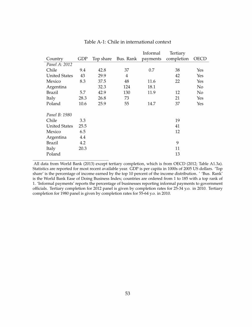
Table A-1: Chile in international context

Informal TertiaryCountry GDP Top share Bus. Rank payments completion OECDPanel A: 2012Chile 9.4 42.8 37 0.7 38 YesUnited States 43 29.9 4 42 YesMexico 8.3 37.5 48 11.6 22 YesArgentina 32.3 124 18.1 NoBrazil 5.7 42.9 130 11.9 12 NoItaly 28.3 26.8 73 21 YesPoland 10.6 25.9 55 14.7 37 Yes

Panel B: 1980Chile 3.3 19United States 25.5 41Mexico 6.5 12Argentina 4.4Brazil 4.2 9Italy 20.3 11Poland 13

All data from World Bank (2013) except tertiary completion, which is from OECD (2012; Table A1.3a).Statistics are reported for most recent available year. GDP is per capita in 1000s of 2005 US dollars. ‘Topshare’ is the percentage of income earned by the top 10 percent of the income distribution. ’ ‘Bus. Rank’is the World Bank Ease of Doing Business Index; countries are ordered from 1 to 185 with a top rank of1. ‘Informal payments’ reports the percentage of businesses reporting informal payments to governmentofficials. Tertiary completion for 2012 panel is given by completion rates for 25-34 y.o. in 2010. Tertiarycompletion for 1980 panel is given by completion rates for 55-64 y.o. in 2010.

53

Table A-2: Leadership roles held by applicants

A. Titles of corporate directorsDirector 0.62Substitute director 0.19President 0.09General manager 0.05Vice President 0.04N 2107

B. Titles of executive managersPrincipal Executive 0.75General Manager 0.24Other 0.01N 1652

C. Assets of SSE companiesFraction listed on SSE 0.3425th percentile 0.350th percentile 0.775th percentile 2.495th percentile 9.7Largest 47.5

D. Assets of non-SSE companiesFraction not listed on SSE 0.6625th percentile 0.0650th percentile 0.475th percentile 1.295th percentile 5.9Largest 44.4

Sample: applicants to elite college programs who rise to top management positions. Data at positionlevel. Panels A and B show the fraction of directors and executives, respectively, by title listed on SVSfilings. Panels C and D show the assets (in billions of 2012 USD) for companies that are listed and notlisted on the Santiago Stock Exchange (SSE). I use asset data from December 2012; asset data are availablefor 95 percent of the SSE sample and 32 percent of the non-SSE sample.

54

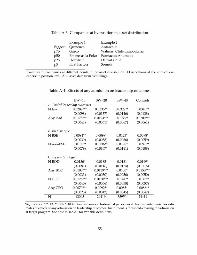
Table A-3: Companies at by position in asset distribution

Example 1 Example 2Biggest Quinenco Antarchilep75 Gasco Walmart Chile Inmobiliariap50 Empresas la Polar Farmacias Ahumadap25 Hortifrut Detroit Chilep5 First Factors Somela

Examples of companies at different points in the asset distribution. Observations at the application-leadership position level. 2011 asset data from SVS filings.

Table A-4: Effects of any admission on leadership outcomes

BW=10 BW=20 BW=40 ControlsA. Pooled leadership outcomesN lead 0.0282*** 0.0335** 0.0322** 0.0343**

(0.0098) (0.0137) (0.0146) (0.0138)Any lead 0.0175*** 0.0194*** 0.0156** 0.0200***

(0.0041) (0.0061) (0.0067) (0.0061)

B. By firm typeN BSE 0.0094** 0.0099* 0.0123* 0.0098*

(0.0039) (0.0058) (0.0066) (0.0059)N non-BSE 0.0189** 0.0236** 0.0198* 0.0246**

(0.0079) (0.0107) (0.0111) (0.0108)

C. By position typeN BOD 0.0156* 0.0185 0.0181 0.0199*

(0.0081) (0.0116) (0.0124) (0.0116)Any BOD 0.0103*** 0.0139*** 0.0100* 0.0150***

(0.0033) (0.0050) (0.0056) (0.0050)N CEO 0.0126*** 0.0150*** 0.0141** 0.0145**

(0.0040) (0.0056) (0.0058) (0.0057)Any CEO 0.0079*** 0.0092** 0.0085* 0.0086**

(0.0023) (0.0042) (0.0045) (0.0042)N 13043 24419 35950 24419

Significance: ***: 1% **: 5% *: 10%. Standard errors clustered at person level. Instrumental variables esti-mates of effects of any admission on leadership outcomes. Instrument is threshold-crossing for admissionat target program. See note to Table 3 for variable definitions.

55

Table A-5: Effects of any admission on leadership outcomes by high school type

I. Elite Private II. Not Elite Private III. Public Exam Test: I vs. IIA. Pooled leadership outcomesN lead 0.1413** 0.0089 0.0231 0.0553*

(0.0678) (0.0135) (0.0326)Any lead 0.0547** 0.0085 0.004 0.0965*

(0.0272) (0.0059) (0.0179)

B. By firm typeN BSE 0.0591* -0.0026 -0.0142 0.0629*

(0.0329) (0.0046) (0.0163)N non-BSE 0.0822* 0.0115 0.0373 0.1388

(0.0464) (0.0113) (0.0283)

C. By position typeN BOD 0.0919 0.0029 0.0016 0.1481

(0.0605) (0.0116) (0.0114)Any BOD 0.0276 0.0035 0.0016 0.292

(0.0224) (0.0045) (0.0114)N CEO 0.0493** 0.006 0.0215 0.0477**

(0.0212) (0.0055) (0.0297)Any CEO 0.0442** 0.0062 -0.0028 0.0666*

(0.0203) (0.0042) (0.0148)N 1513 6965 562

Significance: ***: 1% **: 5% *: 10%. Standard errors clustered at person level. Instrumental variablesestimates of effects of any admission from BW=10 specification. ‘Not elite private’ pools data for allschools that are not elite private high schools. The ‘public exam’ category is the subset of applicationsfrom the column II for students from public exam schools. p-value column reports tests of equality ofcoefficients for students from elite private high schools and other students.

56

Table A-6: Effects of any admission on leadership outcomes by high school type

BW=20 BW=40Elite Private Non-elite p-value Elite private Non-elite p-value

N lead 0.0881 0.0029 0.146 0.0893 -0.0007 0.1714(0.0576) (0.0106) (0.0650) (0.0108)

Any lead 0.0294 0.0043 0.2748 0.0243 -0.0011 0.3184(0.0224) (0.0052) (0.0249) (0.0058)

N SSE 0.0372 -0.0048 0.128 0.0371 -0.0054 0.1956(0.0273) (0.0041) (0.0326) (0.0045)

N non-SSE 0.0509 0.0077 0.2806 0.0522 0.0047 0.2794(0.0391) (0.0089) (0.0430) (0.0089)

N BOD 0.06 -0.0025 0.2414 0.0561 -0.0025 0.3299(0.0526) (0.0089) (0.0595) (0.0090)

Any BOD 0.0211 0.0028 0.3493 0.0115 0.0002 0.6037(0.0191) (0.0042) (0.0213) (0.0047)

N CEO 0.0282 0.0054 0.2124 0.0332* 0.0018 0.1279(0.0176) (0.0049) (0.0200) (0.0050)

Any CEO 0.0212 0.0025 0.2529 0.0254 -0.0004 0.1469(0.0160) (0.0036) (0.0174) (0.0040)

N 2855 13156 4015 19107

Significance: ***: 1% **: 5% *: 10%. Standard errors clustered at person level. Estimates of admissionseffects from BW=20 and BW=40 specifications. ‘Non-elite’ column includes data from students who didnot attend elite private high schools. p-value column reports tests of equality of coefficients for studentsfrom elite and non-elite high schools.

57

Table A-7: Co-leadership rates for admitted and non-admitted students

College peers Same deg., dif. coh. Dif. deg., same coh.A. Within 40 points of cutoffAdmitted 12.54** 2.6 1.43

(5.60) (2.56) (2.67)N 455459 1703535 440509Test 0.0591 0.0426

B. Within 10 points of cutoffAdmitted 12.96 4.15 1.18

(8.77) (4.95) (4.52)N 165304 611947 157109Test 0.2578 0.2272

Significance: ***: 1% **: 5% *: 10%. Standard errors computed using two-way clustering at the personby person level. Coefficients are estimated effects of admission on co-leadership rates per 100,000 pairs.‘College peers’ are students admitted to applicants’ target degree program within one application year.‘Same degree, different cohort’ are students admitted to applicants’ target degree program in more distantapplication years. ‘Different degree, same cohort’ are students admitted to different degree programs inthe same field within one application year. ‘Test’ row provides p-values for tests of equality between the‘college peers’ coefficient and the coefficient listed in the column label.

58

Table A-8: Mean co-leadership rates for student pairs, by type of pair

I. Different HS II. Only marginalA. Within same degree E-E Cd E-E CdClose cohort 8.7** 0.10 12.7** 0.09

(4.4) (5.7)Constant 11.5*** 13.6***

(3.0) (3.5)N 631626 413724

B. Within same fieldSame degree × close cohort 12.4*** 0.14 14.6** 0.14

(4.7) (5.7)Same degree 1.7 1.6

(2.3) (5.3)Close cohort -3.7 -8.2*

(2.6) (4.8)Constant 9.8*** 11.9***

(2.1) (4.3)N 1265996 520481

Significance: ***: 1% **: 5% *: 10%. Standard errors use two-way clustering at student by student level.‘E-E’ columns report co-leadership rates for pairs of admitted students from elite private high schools per100,000 pairs. Cd column reports total connections effects for elite private high school students implied byestimates of co-leadershp rates. Columns under heading I report results for student pairs where studentsattended different high schools. Columns under heading II report results for student pairs where at leastone student had a score within 20 points of the admissions threshold.

B Data appendix

B.1 Data construction and description of the applicant sample

This subsection provides more detail on data availability by year and describes the sam-ple of students applying to elite degree programs.

Table B1 describes data availability for each of the six elite degree programs by year.Data is missing in some years because newspaper records could not be located. Out of168 total program-year cells between 1968 and 1995, I have data on 131. Most of themissing cells are due to the fact that PUC applications do not become available until

59

1976. The rightmost columns shows the total number of programs for which I have ap-plication data for the years 1982 through 1988. I use this data to describe characteristicsof applicants and business leaders in Table 1.

Table B-1: Data availability by year

PUC law PUC Eng. PUC Bus. UC Law UC Eng. UC Bus. N total1968 0 0 0 1 0 11969 0 0 0 1 0 01970 0 0 0 1 1 11971 0 0 0 1 1 11972 0 0 0 1 1 11973 0 0 0 1 1 01974 0 0 0 1 1 11975 0 0 0 0 0 11976 1 1 1 1 1 11977 1 1 1 1 1 11978 1 1 1 1 1 11979 1 1 1 1 1 11980 1 1 1 1 1 11981 1 1 1 1 1 11982 1 1 1 1 1 1 4501983 1 1 1 1 1 1 4601984 1 1 1 1 1 1 4751985 1 1 1 1 1 1 4351986 1 1 1 1 1 1 4311987 0 0 0 1 1 1 4281988 1 1 1 1 1 11989 1 1 1 1 1 11990 1 1 1 1 1 11991 1 1 1 1 1 11992 1 1 1 1 1 11993 1 1 1 1 1 11994 0 0 1 1 1 11995 1 1 1 0 0 1

Data availability by degree program and application year. 1 indicates data is available for a program-yearcell. 0 indicates it is not. ‘N total’ column counts number of total degree programs observed between 1982and 1988.

Table B2 describes the sample of applicants to elite degree programs between 1974 and1995. I match 68,793 applications (unique at the person-degree program-year level) tounique person identifiers. Beginning in 1989, these identifiers were printed in the news-paper alongside application results. For the years 1974 through 1988, I obtain these rutsby matching printed results to administrative application records based on a uniqueapplication identifier. Acceptances account for 53.1 percent of the application sample.The balance between accepted and rejected applicants reflects the fact that schools typ-ically publish a waitlist of equal length to the list of accepted students. 75.5 percent ofapplicants are male, and applicants have an average weighted application score of 682

60

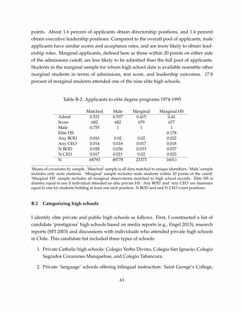
points. About 1.6 percent of applicants obtain directorship positions, and 1.4 percentobtain executive leadership positions. Compared to the overall pool of applicants, maleapplicants have similar scores and acceptance rates, and are more likely to obtain lead-ership roles. Marginal applicants, defined here as those within 20 points on either sideof the admissions cutoff, are less likely to be admitted than the full pool of applicants.Students in the marginal sample for whom high school data is available resemble othermarginal students in terms of admissions, test score, and leadership outcomes. 17.8percent of marginal students attended one of the nine elite high schools.

Table B-2: Applicants to elite degree programs 1974-1995

Matched Male Marginal Marginal HSAdmit 0.531 0.537 0.415 0.41Score 682 682 679 677Male 0.755 1 1 1Elite HS 0.178Any BOD 0.016 0.02 0.02 0.022Any CEO 0.014 0.018 0.017 0.018N BOD 0.028 0.036 0.033 0.037N CEO 0.017 0.021 0.02 0.023N 68793 49778 23373 16011

Means of covariates by sample. ‘Matched’ sample is all data matched to unique identifiers. ‘Male’ sampleincludes only male students. ‘Marginal’ sample includes male students within 20 points of the cutoff.‘Marginal HS’ sample includes all marginal observations matched to high school records. Elite HS isdummy equal to one if individual attended an elite private HS. ‘Any BOD’ and ‘Any CEO’ are dummiesequal to one for students holding at least one such position. N BOD and and N CEO count positions.

B.2 Categorizing high schools

I identify elite private and public high schools as follows. First, I constructed a list ofcandidate ‘prestigious’ high schools based on media reports (e.g., Engel 2013), researchreports (SPI 2003) and discussions with individuals who attended private high schoolsin Chile. This candidate list included three types of schools:

1. Private Catholic high schools: Colegio Verbo Divino, Colegio San Ignacio, ColegioSagrados Corazones Manquehue, and Colegio Tabancura.

2. Private ‘language’ schools offering bilingual instruction: Saint George’s College,

61

the Grange School, Scuola Italiana, Allianza Francesa, Colegio Aleman, ColegioSuizo, and Craighouse School.

3. Public exam schools: Instituto Nacional General Jose Miguel Carrera.

Each of these schools is located in Santiago, and some are all male. The private highschools on this list place highly in rankings based on test scores (see PUC 2012). Moreimportantly, however, attendance at schools within what Contardo (2008) describes as‘the Ivy League of Santiago’ connotes social pedigree. As discussed in Neilson (2013),tuition at these high schools is similar to tuition at elite private high schools in the U.S.as a fraction of per capita GDP. Within the list of elite private schools, it is possibleto construct a loose prestige ranking: Verbo Divino, San Ignacio, Saint George’s, theGrange School, Tabancura, and Manquehue generally place at the top of high schoolsranked by business success of graduates (SPI 2003; Engel 2013). The Instituto Nacionalis clearly the top public school in Chile. Instituto Nacional students score higher thanstudents from any other public school on college entrance examinations (PUC 2012), andthe school counts 17 Chilean presidents (out of 35) amongst its alumni.

I obtain high school data from administrative DEMRE records for the years 1974 through1988. These records include high school codes for 92 percent of applicants in the yearsI study, but high school names are not provided and identification codes change fromyear to year. I identify high schools by constructing a biographical dataset on prominentChileans who applied to college during the period in question. I link this dataset to col-lege applications, and identify high schools based on the biographical dataset.28 I counta high school as having been successfully identified if I match at least two biographicalrecords from different coding regimes to that high school. I link high school codes acrossyears using data on students who re-apply. This procedure allows me to identify eachof the schools listed above except for Colegio Aleman and Colegio Suizo. To extent thatthis process fails to identify or falsely identifies elite private high schools, this shouldtend to lessen differences between elite high school students and other students.

My core finding of heterogeneous effects for students from elite private high schools isrobust to subsetting on different groups of elite private high schools. Table B3 showsestimates of equation 1 in the BW=10 specification for three definitions of elite private

28I delete the biographical dataset following the merge so that I do not observe academic records forincluded individuals.

62

high school. ‘Group 1’ includes the four older schools in the loose ‘highest prestige’category defined above: Verbo Divino, St. George’s, the Grange, and San Ignacio. Theseaccount for roughly two thirds of the elite private high school applicants in my sample.‘Group 2’ adds Tabancura and Manquehue. ‘Group 3’ includes all elite private schools,reproducing results from Table 4 in the text.

Table B-3: Effects of admission on leadership outcomes by high school group

Group 1 Group 2 AllPrep 0.0709* 0.0754* 0.0760**

(0.0420) (0.0408) (0.0365)1032 1311 1513

Non-Prep 0.0126 0.0082 0.0058(0.0096) (0.0088) (0.0088)

7446 7167 6965

Significance: ***: 1% **: 5% *: 10%. Estimates of equation 1 for different subsets of elite private highschools. Group 1 consists of Verbo Divino, St. George’s, Grange, and San Ignacio. Group 2 adds Tabancuraand Manquehue. ‘All’ column uses all available elite private high schools and reproduces estimates fromTable 4.

C Optimal bandwidth and polynomial selection

This appendix considers the selection of optimal polynomial controls and bandwidthsfor regression discontinuity analysis. I first consider the selection of optimal polyno-mial controls. Panel A of Table C1 presents AIC values for estimates of equation 1 us-ing number of leadership positions as the dependent variable, broken down by studentpopulation, bandwidth choice, and polynomial degree. In each case, coefficients onpolynomial terms are allowed to vary above and below the admissions threshold. Atbandwidths of ten and twenty points, the AIC is minimized in all samples with a zero-degree polynomial; i.e., a simple mean comparison. At at 40 point bandwidth, a simplemean comparison minimizes the AIC in both of the high school subsamples, while afirst degree polynomial minimizes the AIC in the pooled sample.

That the optimal polynomial degree is often zero is unsurprising given how flat lead-ership outcomes are in scores; see, e.g., Figures 3 and 4. This is somewhat atypical in

63

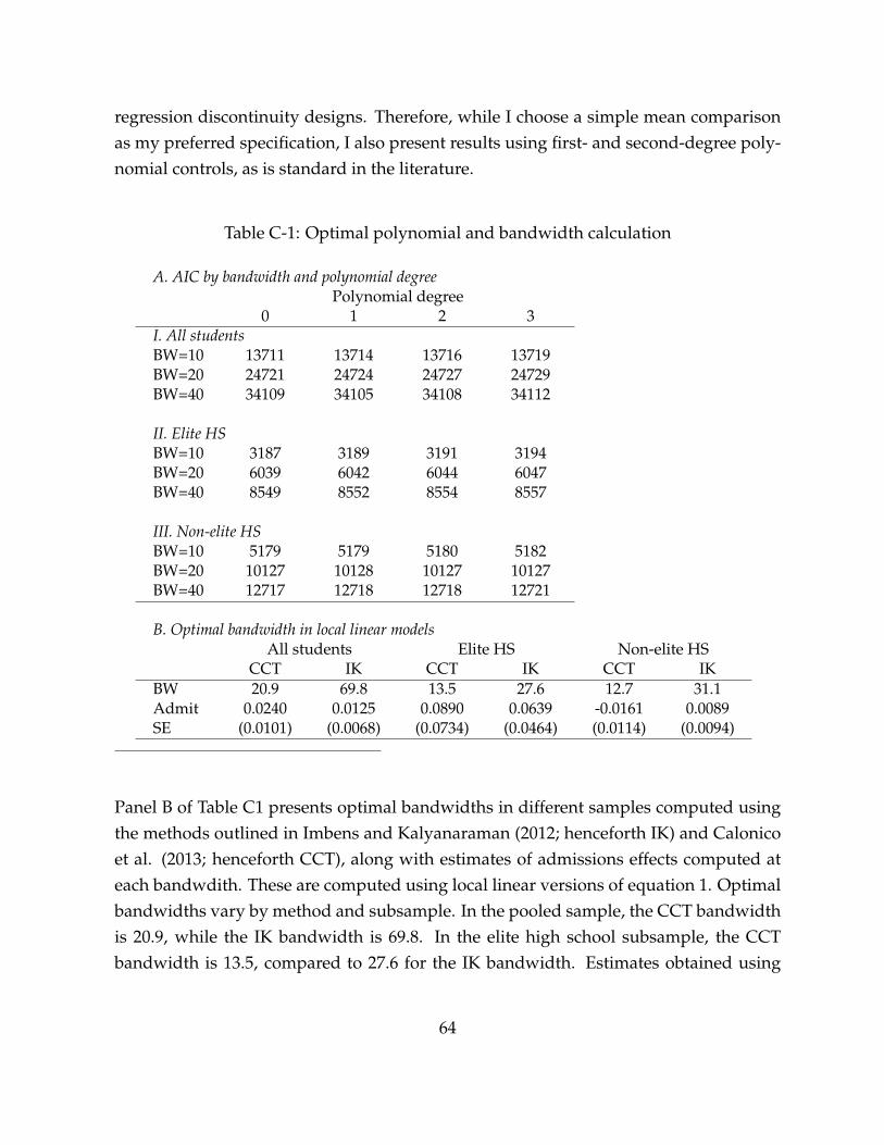
regression discontinuity designs. Therefore, while I choose a simple mean comparisonas my preferred specification, I also present results using first- and second-degree poly-nomial controls, as is standard in the literature.

Table C-1: Optimal polynomial and bandwidth calculation

A. AIC by bandwidth and polynomial degreePolynomial degree

0 1 2 3I. All studentsBW=10 13711 13714 13716 13719BW=20 24721 24724 24727 24729BW=40 34109 34105 34108 34112

II. Elite HSBW=10 3187 3189 3191 3194BW=20 6039 6042 6044 6047BW=40 8549 8552 8554 8557

III. Non-elite HSBW=10 5179 5179 5180 5182BW=20 10127 10128 10127 10127BW=40 12717 12718 12718 12721

B. Optimal bandwidth in local linear modelsAll students Elite HS Non-elite HS

CCT IK CCT IK CCT IKBW 20.9 69.8 13.5 27.6 12.7 31.1Admit 0.0240 0.0125 0.0890 0.0639 -0.0161 0.0089SE (0.0101) (0.0068) (0.0734) (0.0464) (0.0114) (0.0094)

Panel B of Table C1 presents optimal bandwidths in different samples computed usingthe methods outlined in Imbens and Kalyanaraman (2012; henceforth IK) and Calonicoet al. (2013; henceforth CCT), along with estimates of admissions effects computed ateach bandwdith. These are computed using local linear versions of equation 1. Optimalbandwidths vary by method and subsample. In the pooled sample, the CCT bandwidthis 20.9, while the IK bandwidth is 69.8. In the elite high school subsample, the CCTbandwidth is 13.5, compared to 27.6 for the IK bandwidth. Estimates obtained using

64

optimal bandwidths in local linear specifications are generally very similar to those re-ported in the local linear BW=20 specifications; see Tables 3 and A6. The exception is thepooled-sample IK estimate, for which the optimal bandwidth is extremely wide relativeto that computed using the CCT method or using the IK method in other samples.

D Model extension to match heterogeneity

This section extends the model described in section 5.1 to allow for heterogeneous skillmatch between firms and degree programs and between firms and cohorts. The pres-ence of separable degree-firm and cohort-firm match effects motivates the difference-in-differences empirical approach presented in section 5.2 as well as the restriction towithin-field comparisons of admissions effects at the beginning of section 5.

Model setup is as described in section 5.1, with three changes. First, students attendelite or non-elite degree programs in T different cohorts, denoted by t. Second, skillsare firm-specific, and may depend on which elite degree program a student attendsand when. The probability a student from high school type d in cohort t who does notattend an elite degree degree program is productive at firm f is γdt f . If that studentattends an elite college, the probability he is productive at f rises to γdt f + bdp f . Theskill gains from admission to a particular elite degree program for each high school typeare constant within firms over time. Third, referrals occur only within degree-program-cohort groups; i.e., within students who attend the same degree program at the sametime. The probability that there is a type d referral-provider for firm f in elite degreeprogram p and cohort t is again rd.

Let Yidpt f be a dummy variable equal to one if student i from high school type d attend-ing elite degree program p in cohort t is hired at f , and let Yid0t f be a dummy equalto one if i from high school type d in cohort t attending a non-elite degree program ishired at f . Define ∆pt

d as the gain from admission to elite degree program p rather thana non-elite degree program for a cohort-t student. Then we may write

65

∆ptd = E[∑

f(Yidpt f −Yid0t f )|d]

= F×(

bdp f π + rd(γdt f + bdp f )(1− π))

= Sptd + Cpt

d (D.1)

where bdp f = F−1 ∑ f bdp f , γdt f = F−1 ∑ f γdt f , Sptd = Fbdp f π, and Cpt

d = Frd(γdt f +

bdp f )(1−π). As above, we can think of Sptd and Cpt

d as reflecting the skill and connectionscontributions, respectively, to the total effect.

Now consider the first model implication, which held that the admissions gains in co-leadership rates with non-peers were equal to zero if skill gains were zero, and thatadmissions gains in co-leadership rates with peers were equal to gains with non-peersplus a term that depended on network gains rd. Let µ

dp′t′

dpt = E[∑ f Yidpt f Yjdp′t′ f |d, i 6= j

]be the expected co-leadership rate for a pair of high school d students at elite degreeprograms p and p′ in cohorts t and t′. Further, let µ

dp′t′

d0t be expected co-leadership ratefor a high school type d student in cohort t who is not admitted to an elite program andsome student with high school-program-cohort category dp′t′. Then for some programp′ 6= p, we may write

κdp′tdpt = µ

dp′tdpt − µ

dp′td0t

= Fπbdp f (γdt f + bdp′ f ) (D.2)

where bdp f (γdt f + bdp′ f ) = F−1 ∑ f bdp f (γdt f + bdp′ f ). This is the gain in co-leadershiprates with students from other degree programs in the same cohort associated with eliteadmission. Similarly,

κdpt′

dpt = µdpt′

dpt − µdpt′

d0t

= Fπbdp f (γdt′ f + bdp f ) (D.3)

66

while

κdptdpt = µ

dptdpt − µ

dptd0t

= F(1− π)rd(γdt f + bdp f

)2+ Fπbdp f (γdt f + bdp f ). (D.4)

Equations D2 and D3 show the gains in co-leadership rates with students who are notcollege peers associated with elite college admission. As in the model without matcheffects, these gains would be zero if elite colleges do not make students more likely tobe productive; i.e., if the bdp f = 0 for each dp f triplet. Equation D4 shows the gains inco-leadership rates with college peers associated with elite admission. As in the modelwithout match effects, these gains include a peer connections term that is positive onlyif rd > 0, as well as a skill effect term. However, in contrast to the simpler model, theskill effect term in κ

dptdpt is not the same as the skill effect terms in κ

dp′tdpt and κ

dpt′

dpt . Inthe former case, the skill effect terms will differ if bdp f 6= bdp′ f ; i.e., if different degreeprograms teach students different skills. In the latter case, the skill effect terms willdiffer if γdt f 6= γdt′ f . In my empirical work, I take steps to reduce the impact of thesetypes of heterogeneity by considering only pairs of students within the same fields ofstudy, and by considering pairs of students from nearby cohorts.

I now turn to the second model implication, which provided a formula for the con-nections effect term Cd. A similar result goes through here based on a difference-in-differences approach. Specifically, we may define

τptd =

((µ

dptdpt − µ

dpt′

dpt

)−(

µdp′tdpt − µ

dp′t′

dpt

))= F(1− π)rd

(γdt f + bdp f

)2 (D.5)

This difference-in-differences approach isolates a term that is proportional to total peereffect contribution Cpt

d . The single-difference approach outlined in the model withoutmatch effects fails because of cohort match effects (for differences within degree pro-grams across cohorts) and skill match effects (for differences across degree programs

67

within cohorts).

As in the model presented in the main text, it is possible to rescale the difference-in-differences estimates using observable quantities to recover overall gains from peer ef-fects. Let Cd = Ept[C

ptd |d] and τd = Ept[τ

ptd |d] be the average total peer effect and the

difference-in-differences estimate of peer co-leadership effects, respectively, across alldegree programs and cohorts. Then

Cd = τd ×Eipt[∑ f Yidpt f |d]

Eijpt[∑ f Yidpt f Yjdpt f |d, i 6= j](D.6)

as before.

E Standard errors in peer effects analysis

I estimate equations six and seven using paired data that is unique at the applicationby application level. A priori it is not clear how best to compute standard errors. Lead-ership error terms are most likely correlated within all observations for the same indi-vidual. It is also reasonable to think that errors might be correlated across observationswithin the same program cohort, since students within program-cohort cells have accessto the same or similar peer contacts. Prior studies using similar data have taken a varietyof approaches. Bayer et al. (2008) compute standard errors using a pairwise bootstrap.Shue (2013) presents results using both two-way clustering at the person-person level(as in Cameron et al. 2011 or Peterson 2009) and a non-parametric placebo test. Thetwo procedures yield similar results. Fracassi (2012) uses data on pairs of firms, andcomputes standard errors using two-way clustering at the firm-firm level.

In the main text, I present standard errors that allow for two-way clustering at theperson-person level. To check that inference is not compromised by error correlationswithin peer groups, I present alternate estimates that allow for two-way clustering atthe program-year by program-year and field-year by field-year level in Table E1 below.Standard errors computed using do not materially change inferences drawn in the maintext.

68

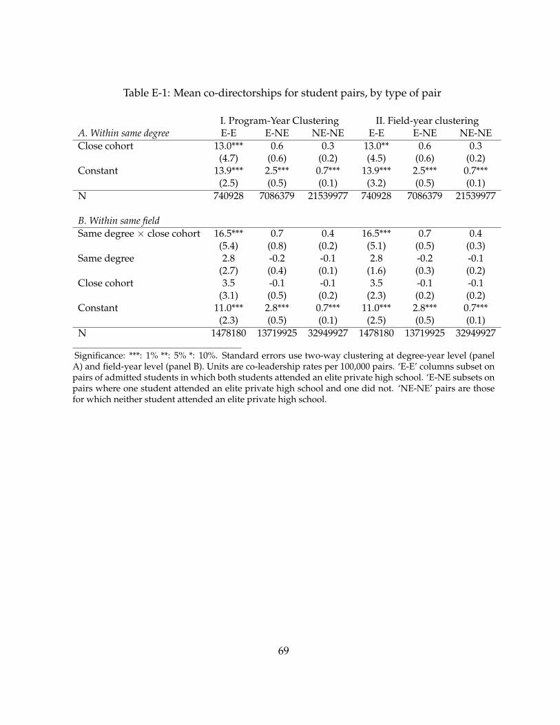
Table E-1: Mean co-directorships for student pairs, by type of pair

I. Program-Year Clustering II. Field-year clusteringA. Within same degree E-E E-NE NE-NE E-E E-NE NE-NEClose cohort 13.0*** 0.6 0.3 13.0** 0.6 0.3

(4.7) (0.6) (0.2) (4.5) (0.6) (0.2)Constant 13.9*** 2.5*** 0.7*** 13.9*** 2.5*** 0.7***

(2.5) (0.5) (0.1) (3.2) (0.5) (0.1)N 740928 7086379 21539977 740928 7086379 21539977

B. Within same fieldSame degree × close cohort 16.5*** 0.7 0.4 16.5*** 0.7 0.4

(5.4) (0.8) (0.2) (5.1) (0.5) (0.3)Same degree 2.8 -0.2 -0.1 2.8 -0.2 -0.1

(2.7) (0.4) (0.1) (1.6) (0.3) (0.2)Close cohort 3.5 -0.1 -0.1 3.5 -0.1 -0.1

(3.1) (0.5) (0.2) (2.3) (0.2) (0.2)Constant 11.0*** 2.8*** 0.7*** 11.0*** 2.8*** 0.7***

(2.3) (0.5) (0.1) (2.5) (0.5) (0.1)N 1478180 13719925 32949927 1478180 13719925 32949927

Significance: ***: 1% **: 5% *: 10%. Standard errors use two-way clustering at degree-year level (panelA) and field-year level (panel B). Units are co-leadership rates per 100,000 pairs. ‘E-E’ columns subset onpairs of admitted students in which both students attended an elite private high school. ‘E-NE subsets onpairs where one student attended an elite private high school and one did not. ‘NE-NE’ pairs are thosefor which neither student attended an elite private high school.

69

making top managers: the role of elite universities and ......dents from nearby cohorts in that...

Documents