No. 09‐1 

 

Making Sense of the Subprime Crisis 

Kristopher S. Gerardi, Andreas Lehnert, Shane M. Sherlund,   

and Paul S. Willen 

Abstract: This paper  explores  the question of whether market participants  could have or  should have anticipated the large increase in foreclosures that occurred in 2007 and 2008. Most of these foreclosures stem from loans originated in 2005 and 2006, leading many to suspect that  lenders  originated  a  large  volume  of  extremely  risky  loans  during  this  period. However, the authors show that while loans originated in this period did carry extra risk factors, particularly increased leverage, underwriting standards alone cannot explain the dramatic  rise  in  foreclosures.  Focusing  on  the  role  of  house  prices,  the  authors  ask whether market participants underestimated the likelihood of a fall in house prices or the sensitivity of  foreclosures  to house prices. The authors  show  that, given available data, market participants  should have been able  to understand  that a  significant  fall  in prices would  cause  a  large  increase  in  foreclosures,  although  loan‐level  (as  opposed  to ownership‐level) models would  have  predicted  a  smaller  rise  than  actually  occurred. Examining analyst reports and other contemporary discussions of the mortgage market to see what market participants  thought would happen,  the authors  find  that analysts, on the whole, understood  that a  fall  in prices would have disastrous consequences  for  the market but assigned a low probability to such an outcome. 

JEL Classifications: D11, D12, G21    Kristopher  S. Gerardi  is  a  research  economist  and  assistant policy  advisor  at  the Federal Reserve Bank of 

Atlanta.  Andreas Lehnert is chief of the household and real estate finance section and Shane M. Sherlund is a 

senior  economist  in  the  household  and  real  estate  finance  section,  both  in  the  division  of  research  and 

statistics at the Board of Governors of the Federal Reserve System.   Paul S. Willen is a senior economist and 

policy  advisor  at  the  Federal  Reserve  Bank  of  Boston.  The  authors’  email  addresses  are, 

kristopher.gerardi@atl.frb.org, andreas.lehnert@frb.gov, shane.m.sherlund@frb.gov, and 

paul.willen@bos.frb.org, respectively. 

 This  paper, which may  be  revised,  is  available  on  the web  site  of  the  Federal Reserve Bank  of Boston  at http://www.bos.frb.org/economic/ppdp/index.htm. 

The opinions and analysis  in  this paper are  solely  those of  the authors and not  the official position of  the Federal Reserve Bank of Boston, the Federal Reserve Bank of Atlanta, or the Federal Reserve System. 

This paper was prepared  for  the Brookings Panel on Economic Activity, September 11–12, 2008. We  thank Debbie  Lucas  and  Nick  Souleles  for  excellent  discussions,  the  editors  for  their  suggestions,  advice,  and patience, and the Brookings Panel and various other academic and non‐academic audiences for their helpful comments. We thank Christina Pinkston for valuable help programming the First American LoanPerformance data. Any remaining errors are our own responsibility. 

 

This version: December 22, 2008 

1 Introduction

Had market participants anticipated the increase in defaults on subprime mortgages

originated in 2005 and 2006, the nature and extent of the current financial market dis-

ruptions would be very different.Ex ante, investors in subprime mortgage-backed

securities would have demanded higher returns and greater capital cushions. As a re-

sult, borrowers would not have found credit as cheap or as easy to obtain as it became

during the subprime credit boom of 2005–2006. Rating agencies would have had a

similar reaction, rating a much smaller fraction of each deal investment grade.Ex post,

the increase in foreclosures would have been significantly smaller, with fewer attendant

disruptions to the housing market. In addition, investors would not have suffered such

outsized, and unexpected, losses. To make sense of the subprime crisis, one needs to

understand why, when accepting significant exposure to the creditworthiness of sub-

prime borrowers, so many smart analysts, armed with advanced degrees, data on the

past performance of subprime borrowers, and state-of-the-art modeling technology did

not anticipate that so many of the loans they were buying, either directly or indirectly,

would go bad.

Our bottom line is that the problem largely had to do with house price expectations.

Had investors known the trajectory of house prices, they would have predicted large in-

creases in delinquency and default and losses on subprime mortgage-backed securities

(MBS) roughly consistent with what we have seen. We show this by using two differ-

ent methods to travel back to 2005, when subprime was still thriving, and look forward.

The first method is to forecast performance with only data available in 2005 and the

second is to look at what market participants wrote at the time. The latter “narrative”

analysis, which appears in Section 4 below, provides strong evidence against the claim

that investors lost money by purchasing loans which, because they were originated by

others, could not be evaluated properly.

We proceed by first addressing the question of whether the loans themselves were

ex anteunreasonable. Loans made in 2005–2006 were not that different from loans

made earlier, which, in turn had performed well, despite carrying a variety of serious

risk factors. We show that lenders did make riskier loans, and describe in detail the

dimensions along which risk increased. In particular, we find that borrower leverage

increased and, further, did so in a way that was relatively opaque to investors. However,

2

we find that the change in the mix of mortgages originated is too mild to explain the

huge increase in defaults. Put simply, the average default rate on loans originated in

2006 exceeds the default rate on the riskiest category of loans originated in 2004.

We then focus on the collapse in house price appreciation (HPA) that started in the

spring of 2006.1 Lenders must either have expected that HPA would remain high (or

at least that house prices would not collapse), or have expected subprime defaults to

be insensitive to a big drop in house prices. More formally, if we letf represent fore-

closures,p represent prices, andt represent time, then we can decompose the growth

in foreclosures over time,df/dt, into a part corresponding to the change in prices over

time and a part reflecting the sensitivity of foreclosures to prices:

df/dt = df/dp × dp/dt.

Our goal is to determine whether market participants underestimateddf/dp, the sensi-

tivity of foreclosures to prices, or whetherdp/dt, the trajectory of house prices, came

out much worse than they expected.

We begin with data that were available,ex ante,on mortgage performance to de-

termine whether it was possible to estimatedf/dp on subprime mortgages accurately.

Because severe house price declines are relatively rare and the subprime market is rel-

atively new, one plausible theory is that the data did not contain sufficient variation to

estimatedf/dp in scenarios in whichdp/dt is negative and large. We put ourselves

in the place of analysts in 2005, using data through 2004 to estimate the type of haz-

ard models commonly used in the industry to predict mortgage defaults. We use two

datasets. The first is a loan-level dataset from First American LoanPerfomance that

is used extensively in the industry to track the performance of mortgages in MBS;

this dataset has sparse information on loans originated before 1999. The second is an

ownership-level dataset from the Warren Group, which tracked the fates of homebuy-

ers in Massachusetts from the late 1980s forward. These data were not (so far as we

can tell) widely used by industry but were, at least in theory, available. The Warren

Group data do contain information on the behavior of homeowners in an environment

of falling prices.

We find that it was possible, although not easy, to measuredf/dp with some degree

1Examples include Gerardi, Shapiro, and Willen (2007), Mayer, Pence, and Sherlund (2008), Demyanykand van Hemert (2007), Doms, Furlong, and Krainer (2007), and Danis and Pennington-Cross (2005).

3

of accuracy. Essentially, a researcher with perfect foresight about the trajectory of

prices from 2005 forward would have forecast a large increase in foreclosures starting

in 2007. Perhaps the most interesting result is that, despite the absence of negative

HPA in 1998–2004, when almost all subprime loans were originated, we could still

determine, albeit not exactly, the behavior of subprime borrowers in a falling house

price environment. In effect, the out-of-sample (and out-of-support) performance of

default models was sufficiently good to have predicted large losses in a falling house

price environment.

However, while it was possible to estimatedf/dp, we also find that the relationship

was less exact when using data onloans rather than data onownerships. A given

borrower might refinance his original loan several times before defaulting. All of the

loans bar the final one would have been seen as successful by lenders. An ownership

spans multiple loans and terminates only when the homeowner sells and moves or is

foreclosed upon and evicted. Thus, while the same foreclosure would appear as a

default in both loan-level and ownership-level data, intermediate refinancings between

purchase and foreclosure would not appear as happy endings in an ownership-level

database.

In the last section of the paper, we discuss what analysts of the mortgage market

said in 2004, 2005, and 2006 about the loans that eventually got into trouble. Our

conclusion is that investment analysts had a good sense ofdf/dp and understood, with

remarkable accuracy, how fallingdp/dt would affect the performance of subprime

mortgages and the securities backed by them. As an illustrative example, consider a

2005 analyst report published by a large investment bank: it analyzed a representative

deal composed of 2005 vintage loans and argued it would face 17 percent cumulative

losses in a “meltdown” scenario in which house prices fell 5 percent over the life of the

deal. Their analysis is prescient: the ABX index (an index that represents a basket of

credit default swaps on high-risk mortgages and home equity loans) currently implies

that such a deal will actually face losses of 18.3 percent over its life. The problem was

that the report only assigned a 5 percent probability to the meltdown scenario, whereas

it assigned a 15 percent probability and a 50 percent probability to scenarios in which

house prices grew 11 percent and 5 percent, respectively, over the life of the deal.

We argue that house prices outweigh other changes in driving up foreclosures.

However, we do not take a position on why prices rose so rapidly, fell so fast, and

4

why they peaked in mid-2006. Other researchers have examined whether factors such

as lending standards can affect house prices.2 Broadly speaking, we maintain the

assumption that while, in the aggregate, lending standards may indeed have affected

house price dynamics (we are agnostic on this point), no individual market participant

felt that he could affect prices with his actions. Nor do we analyze whether the housing

market was overvalued in 2005 and 2006, and whether a collapse of house prices was

therefore, to some extent, predictable. There was a lively debate during that period,

with some arguing that housing was reasonably valued (see Himmelberg, Mayer, and

Sinai 2005 and McCarthy and Peach 2004) and others arguing that it was overvalued

(see Gallin 2006, Gallin 2008, and Davis, Lehnert, and Martin 2008).

Our results in Sections 2 and 3 suggest that some borrowers were more sensitive

than others to a single macro risk factor (here: house prices). This comports well with

the findings of Musto and Souleles (2006), who argue that average default rates are

only half the story; they argue that correlations across borrowers, perhaps driven by

macro factors, are also an important factor in valuing portfolios of consumer loans.

In this paper, we focus almost exclusively on subprime mortgages. However, many

of the same arguments might apply to prime mortgages. Lucas and McDonald (2006)

computed the volatility of the underlying assets of the housing-related government-

sponsored enterprises (GSEs), which concentrate mainly on prime and near-prime

mortgages, using information on the firms’ leverage and their stock prices. They found

that risk was quite high (and, as a result, the value of the implicit government guarantee

on GSE debt was also quite high).

Many have argued that a major driver of the subprime crisis was the increased use

of securitization.3 In this view, the “originate to distribute” business model of many

mortgage finance companies separated the underwriter making the credit extension de-

cision from exposure to the ultimate credit quality of the borrower and thus created an

incentive to maximize lending volume without concern for default rates. In addition,

information asymmetries, unfamiliarity with the market, or other factors prevented in-

vestors who were buying the credit risk from putting in place effective controls for these

incentives. While this argument is intuitively persuasive, our results are not consistent

2Examples of this include Pavlov and Wachter (2006), Coleman IV, Lacour-Little, and Vandell (2008),Wheaton and Lee (2008), Wheaton and Nechayev (2008), and Sanders, Chomsisengphet, Agarwal, andAmbrose (2008).

3See, for example, Keys, Mukherjee, Seru, and Vig (2008) and Calomiris (2008).

5

with such an explanation. One of our key findings is that most of the uncertainty about

losses stemmed from uncertainty about the evolution of house prices and not from

uncertainty about the quality of the underwriting. All that said, our models do not per-

fectly predict the defaults that occurred, and these often underestimate the number of

defaults. One possible explanation is that there was an unobservable deterioration of

underwriting standards in 2005 and 2006.4 But another possible explanation is that our

model of the highly non-linear relationship between prices and foreclosures is wanting.

No existing research successfully separates the two explanations.

The endogeneity of prices does present a problem for our estimation. One com-

mon theory is that foreclosures drive price falls by increasing the supply of homes for

sale, in effect introducing a new term into the decomposition ofdf/dt, namely,dp/df .

However, our estimation techniques are, to a large extent, robust to this issue.5 In fact,

as we show in Section 3, it is possible to estimate the effect of house prices on fore-

closures even in periods when there were very few foreclosures, and when foreclosed

properties sold quickly.

No discussion of the subprime crisis of 2007 and 2008 is complete without mention

of the interest rate resets built into many subprime mortgages that virtually guaranteed

large payment increases. Many commentators have attributed the crisis to the payment

shock associated with the first reset of subprime 2/28 mortgages. However, the evi-

dence from loan-level data shows that resets cannot account for a significant portion of

the increase in foreclosures. Both Mayer, Pence, and Sherlund (2008) and Foote, Ger-

ardi, Goette, and Willen (2007) show that the overwhelming majority of defaults on

subprime adjustable-rate mortgages (ARM) occur long before the first reset. In other

words, many lenders would have been lucky had borrowers waited until the first reset

to default.

The rest of the paper is organized as follows. In Section 2, we document changes in

underwriting standards on mortgages. In Section 3 we explore what researchers could

have learned with the data they had in 2005. We review contemporary analyst reports

in Section 4. Section 5 concludes.4An explanation favored by Demyanyk and van Hemert (2007).5As discussed in Gerardi, Shapiro, and Willen (2007), most of the variation in the key explanatory

variable, homeowner’s equity, is within-town (MSA), within-quarter variation, and thus could not be drivenby differences in foreclosures over time or across towns (MSAs)

6

2 Underwriting Standards in the Subprime Market

In this section, we begin with a brief background on subprime mortgages, including the

competing definitions of “subprime.”6 We then turn to a discussion of changes in the

apparent credit risk of subprime mortgages originated from 1999 to 2007, and we link

these to the actual performance of the underlying loans. We argue that the increased

number of subprime loans originated with high loan-to-value rations (LTV) was the

most important observable risk factor that increased over the period. Further, we argue

that the increases in leverage were to some extent masked from investors in mortgage-

backed securities. Loans originated with less than complete documentation of income

or assets, and particularly those originated with both high leverage and incomplete

documentation, exhibited sharper rises in defaults than other loans. A more formal

decomposition exercise, however, confirms that the rise in defaults can be only partly

explained by observed changes in underwriting standards.

2.1 Background on subprime mortgages

One of the first notable features encountered by researchers working on subprime mort-

gages is the dense thicket of jargon surrounding the field, particularly the multiple com-

peting definitions of “subprime.” This hampers attempts to estimate the importance of

subprime lending.

There are, effectively, four useful ways to categorize a loan as subprime. First,

mortgage servicers themselves recognize that certain borrowers require more frequent

contact in order to ensure timely payment; they charge higher fees to service these

loans. Second, some lenders specialize in loans to financially troubled borrowers. The

Department of Housing and Urban Development maintains a list of such lenders. Loans

originated by these so-called “HUD list” lenders are often taken as a proxy for sub-

prime loans. Third, “high cost” loans are defined as loans that carry fees and rates

significantly above those charged to typical borrowers. Fourth, the loan may be sold

into an asset-backed security marketed as containing subprime mortgages.

Table 1 provides two measures of the importance of subprime lending in the United

States. The first column shows the percent of loans in the Mortgage Bankers Associ-

ation (MBA) delinquency survey that are classified as “subprime.” Because the MBA

6For a more detailed discussion, see Mayer and Pence (2008).

7

surveys mortgage servicers, this column represents the servicer definition of a subprime

loan. As shown, over the past few years, subprime mortgages have accounted for about

12 to 14 percentage of outstanding mortgages. The second and third columns show the

percent of loans tracked under the Home Mortgage Disclosure Act that are classified

as “high cost.” As shown, in 2005 and 2006 roughly 25 percent of originations were

subprime under this definition.7

These two measures point to an important discrepancy between thestockand the

flowof subprime mortgages (although source data and definitions also account for some

of the difference). Subprime mortgages were a growing part of the U.S. mortgage

market, so that the flow of new mortgages should naturally exceed their presence in

the stock of outstanding mortgages. In addition, subprime mortgages, for a variety

of reasons, tend to last for a shorter period of time than prime mortgages, so they

form a larger share of the flow of new mortgages than of the stock of outstanding

mortgages. Furthermore, until the mid-2000s most subprime mortgages were typically

used to refinance an existing loan and, simultaneously, to increase the principal balance

(allowing the homeowner to borrow against accumulated equity), rather than to finance

the purchase of a home.

In this section we focus on changes in the kinds of loans made over the period

1999 to 2007. We use loan-level data on mortgages sold into private-label mortgage-

backed securities marketed as subprime. These data are provided by First American

LoanPerformance and were widely used in the financial services industry. We further

limit the set of loans to the three most popular products: those carrying fixed interest

rates to maturity, and so-called “2/28s” and “3/27s.” A 2/28 is a mortgage in which the

contract rate is fixed at an initial “teaser” rate for two years, after which it adjusts to the

six-month Libor rate plus a predetermined margin (often around 6 percentage points).

A “3/27” is similar.8 We refer to this database as “the ABS data” for simplicity.

In this section, the outcome variable of interest is whether a mortgage defaults

within 12 months of its first payment due date. There are several competing definitions

of “default”; here, we define a mortgage as having defaulted by month 12 if, as of

7HMDA data are taken from Federal ReserveBulletin articles; see Avery, Canner, and Cook (2005),Avery, Brevoort, and Canner (2006), Avery, Brevoort, and Canner (2007), and Avery, Brevoort, and Canner(2008). Note that the high-cost measure was only introduced to the HMDA data in 2004; for operational andtechnical reasons, the reported share of high cost loans in 2004 may be depressed relative to its share in lateryears.

8These three loan categories accounted for more than 98 percent of loans in the original data.

8

its twelfth month of life, it had terminated following a foreclosure notice; if the loan

was listed as real estate owned by the servicer (indicating a transfer of title from the

borrower); if the loan was still active but foreclosure proceedings had been initiated;

or if the loan was 90 or more days past due. Note that some of the loans we count

as defaults might subsequently revert to current status if the borrower made up missed

payments. In effect, any borrower who manages to make 10 of the first 12 mortgage

payments or who refinances or sells without a formal notice of default having been

filed is assumednot to have defaulted.

The default rate is shown in Figure 1. Conceptually, default rates differ from delin-

quency rates in that they track the fate of mortgages originated in a given month by

their twelfth month of life; in effect, the default rate tracks the proportion of mort-

gages originated at a given point that are “dead” by month 12. Delinquency rates, by

contrast, track the proportion of all active mortgages that are “sick” at a given point

in calendar time. Further, because we close our dataset in December 2007, we can

track only the fate of mortgages originated through Deccember 2006. The continued

steep increase in mortgage distress is not reflected in our data here, nor is the fate of

mortgages originated in 2007, although we do track the underwriting characteristics of

these mortgages.

Note that this measure of default is designed to allow us to compare theex ante

credit risk of various underwriting terms. It is of limited usefulness as a predictor of

defaults because it considers only what happens by the twelfth month of life and does

not consider the changing house price, interest rate, and overall economic environment

faced by households. Further, this measure does not consider the changing incentives

to refinance. The competing risk, duration models we estimate in Section 3 are, for

these reasons, far better suited to determining the credit and prepayment outlook for a

group of mortgages.

2.2 Changes in underwriting standards

During the credit boom, lenders published daily “rate sheets” with various combina-

tions of loan risk characteristics and the associated interest rates they would charge to

make such loans. A simple rate sheet, for example, might be a matrix of credit scores

and loan-to-value ratios; borrowers with lower credit scores or higher LTVs would be

9

charged higher interest rates or be forced to pay larger fees up front. Certain cells of

the matrix such as combinations of low score and high LTV, might not be available at

all.

Unfortunately, we do not have access to information on the evolution of rate sheets

over time, but underwriting standards can change in ways observable in the ABS data.

Of course, underwriting standards can also change in ways observable to the loan orig-

inator but not reflected in the ABS data, or in ways largely unobservable by even the

loan originator (for example, an increase in the number of borrowers getting home

equity lines of credit (HELOCs) after origination). In this section, we consider the ev-

idence that more loans withex ante, observable risky characteristics were originated.

Throughout, we use loans from the ABS database described earlier.

We consider trends over time in borrower credit scores, loan documentation, lever-

age (as measured by the combined loan-to-value ratio or CLTV at origination), and

other factors associated with risk, such as a loan’s purpose, non-owner occupancy, and

amortization schedules. We find that, from 1999 to 2007, borrower leverage, loans with

incomplete documentation, loans used to purchase homes (as opposed to refinance an

existing loan), and loans with non-traditional amortization schedules grew. Borrower

credit scores increased while loans to non-occupant owners remained essentially flat.

Of these, the increase in borrower leverage appears to have contributed the most to the

increase in defaults, and we find some evidence that leverage was, in the ABS data at

least, opaque.

Credit Scores Credit scores, which essentially summarize a borrower’s history of

missing debt payments, are the most obvious definition of “subprime.” The commonly

used scalar credit score is the FICO score originally developed by Fair, Isaac & Co.

It is the only score contained in the ABS data, although subprime lenders often used

scores and other information from all three credit reporting bureaus.

Under widely accepted industry rules of thumb, borrowers with FICO scores of

680 or above are not usually considered subprime without another accompanying risk

factor; borrowers with credit scores between 620 and 680 may be considered subprime,

while those with credit scores below 620 are rarely eligible for prime loans. Note that

subprime pricing models typically used more information than just a borrower’s credit

score; they also considered the nature of the missed payment that led a borrower to

10

have a low credit score. For example, a pricing system might assign greater weight to

missed mortgage payments than to missed credit card payments.

Figure 2 shows the proportion of newly originated subprime loans falling into each

of these three categories. As shown, loans to borrowers with FICO scores of 680 and

above grew over the sample period, while loans to traditionally subprime borrowers

(those with scores below 620) accounted for a smaller share of originations.

Loan Documentation Borrowers (or their mortgage brokers) submit a file with each

mortgage application documenting the borrower’s income, liquid assets, other debts,

and the value of the property being used as collateral. Media attention has focused on

the rise of so-called “low doc” or “no doc” loans, which contained incomplete docu-

mentation of income or assets. (These are the infamous “stated income” loans.) The

top left panel of Figure 3 shows the proportion of newly originated subprime loans

carrying less than full documentation. As shown, this proportion rose from around 20

percent in 1999 to a high of more than 35 percent by mid-2006. While reduced doc

lending was a part of subprime lending, it was by no means the majority of the business,

nor did it increase dramatically during the credit boom.

As we discuss in greater detail below, until about 2004, subprime loans were gener-

ally backed by substantial equity in the property. This was especially true for subprime

loans with less than complete documentation. Thus, in some sense, the lender accepted

less complete documentation in exchange for a greater security interest in the underly-

ing property.

Leverage The leverage of a property is, in principle, the total value of all liens di-

vided by the mark-to-market value of the property. This is often referred to as the

property’s combined loan-to-value ratio, or CLTV. Both the numerator and denomina-

tor of the CLTV will fluctuate over a borrower’s tenure in the property: the borrower

can amortize the original loan, refinance or take on junior liens, and the potential sale

price of the house will also, of course, change over time. However, all of these vari-

ables ought to be known at the time of a loan’s origination. The lender undertakes a

title search to check for the presence of other liens on the property and hires an ap-

praiser to confirm either the price paid (when the loan is used to purchase a home) or

the potential sale price of the property (when the loan is used to refinance an existing

11

loan).

In practical terms, high leverage was also accompanied by additional complications

and opacity. Rather than originate a single loan for the desired amount, originators

often preferred to originate two loans: one for 80 percent of the property’s value, and

the other for the remaining desired loan balance. In the event of a default, the holder of

the first lien would be paid first from sale proceeds, with the junior lien holder getting

the remaining proceeds (if any). Lenders may have split loans in this way for the same

reason that asset-backed securities are tranched into a AAA-rated piece and a below

investment-grade piece. Some investors might specialize in credit risk evaluation and

hence prefer the riskier piece, while other investors might prefer to forgo credit analysis

and purchase the less risky loan.

The reporting of these junior liens in the ABS data appears to be spotty. This could

be the case if, for example, the junior lien was originated by a different lender than

the first lien, because the first lien lender might not properly report the second lien,

while the second lien lender might not report the loan at all. If the junior lien was an

open-ended loan, such as a home equity line of credit (HELOC), it appears not to have

been reported in the ABS data at all, perhaps because the amount drawn was unknown

at origination.

Further, there is no comprehensive national system for tracking liens on any given

property. Thus, homeowners could take out a second lien shortly after purchasing or

refinancing, raising their CLTV. While such borrowing should not affect the original

lender’s recovery, it does increase the probability of a default and thus the value of the

original loan.

The top right panel of Figure 3 shows the growth in the number of loans originated

with a high CLTV (defined as CLTV≥ 90 percent or the presence of a junior lien);

in addition, the figure shows the proportion of loans originated for which a junior lien

was recorded.9 As shown, both measures of leverage rose sharply over the past decade.

High CLTV lending accounts for roughly 10 percent of originations in 2000, rising to

over 50 percent by 2006. The incidence of junior liens also rose.

The presence of a junior lien has a powerful effect on the CLTV of the first lien.

As shown in Table 2, loans without a second lien reported a CLTV of 79.9 percent,

9The figures shown here and elsewhere are based on first liens only; where there is an associated juniorlien that information is used in computing CLTV and for other purposes, but the junior loan itself is notcounted.

12

while those with a second lien reported a CLTV of 98.8 percent. Moreover, loans with

reported CLTVs of 90 percent or above were much likelier to have associated junior

liens, suggesting that lenders were leery of originating single mortgages with LTVs

greater than 90 percent.

Later, we will discuss the evidence that there was even more leverage than reported

in the ABS data.

Other Risk Factors A variety of other loan and borrower characteristics may have

contributed to increased risk. The bottom left panel of Figure 3 shows the fraction of

loans originated with a non-traditional amortization schedule, to non-occupant owners,

and to borrowers who used the loan to purchase a property (as opposed to refinancing

an existing loan).

A standard, or “traditional,” U.S. mortgage self-amortizes; that is, a portion of

each month’s payment is used to reduce the principal owed on the loan. As shown

in the bottom left panel of Figure 3, non-traditional amortization schedules became

increasingly popular among subprime loans. These were mainly loans that lowered

payments by not requiring sufficient principal payments (at least in the early years of

the loan) to amortize over the 30-year term of the loan. Thus, some loans had interest-

only periods, while others were amortized over 40 years, with a balloon payment due at

the end of the 30-year term. The effect of these terms was to slightly lower payments,

especially in the early years of the loan.

Subprime loans had traditionally been used to refinance an existing loan. As shown

in the bottom left panel of Figure 3, loans used to purchase homes also increased over

the period, although not dramatically. Loans to non-occupant owners, for example,

loans backed by a property held for investment purposes, are, all else equal, riskier

than loans to owner occupiers because the borrower can default and not face eviction

from his primary residence. As shown, such loans never accounted for a large fraction

of subprime originations, nor did they grow over the period.

Risk Layering As we discuss below, leverage is a key risk factor for subprime mort-

gages. An interesting question is the extent to which high leverage loans were com-

bined with other risk factors; this practice was sometimes known asrisk layering.As

shown in the bottom right panel of Figure 3, risk layering grew over the sample period.

13

In particular, loans with incomplete documentationandhigh leverage had an especially

notable rise, increasing from essentially zero in 2001 to almost 20 percent of subprime

originations by the end of 2006. Highly leveraged loans to borrowers purchasing homes

also increased over the period.

2.3 Effect on default rates

We now turn to considering the performance of the various risk factors that we outlined

earlier. We start with simple univariate descriptions before turning to a more formal

decomposition exercise. Here, we continue to focus on 12-month default rates as our

outcome of interest. In the next section we present results from dynamic models that

consider the ability of borrowers to refinance as well as default.

Documentation Level The upper left panel of Figure 4 shows the default rates over

time for loans with complete and incomplete documentation. As shown, the two loan

types performed roughly in line with one another until the current cycle, when default

rates on loans with incomplete documentation rose far more rapidly than default rates

on loans with complete documentation.

Leverage The top right panel of Figure 4 shows default rates on loans with high

CLTVs (defined, again, as a CLTV≥ 90 or having a junior lien present at origination).

Again, loans with high leverage performed approximately in line with other loans until

the most recent episode.

As we highlighted in the earlier discussion, leverage is often opaque. To dig deeper

into the correlation between leverage at origination and subsequent performance, we

estimated a pair of simple regressions relating CLTV at origination to default probabil-

ities and the initial contract interest rate charged to the borrower. The results are shown

in Table 3. For all loans in the sample, we estimated a probit model of default and an

OLS model of the initial contract rate. The list of explanatory variables contained var-

ious measures of leverage, including an indicator variable for having a reported CLTV

in the dataset ofexactly80 percent, as well as a few other controls. We estimated two

versions of the simple model: model 1 simply contains the CLTV measures and the

initial contract rate itself; model 2 adds state and origination-date fixed effects. These

results are designed purely to highlight the correlation among variables of interest and

14

not as fully fledged risk models. Model 1 can be thought of as the simple multivariate

correlation across the entire sample, while model 2 compares loans originated in the

same state at the same time. The results are shown in Figure 6. (When plotting the

expected default probability from model 2, we assume that the loan was originated in

California, in June 2005.)

As shown, default probabilities generally increase with increasing leverage. Note,

however, that loans with reported CLTVs ofexactly80 percent, which account for 15.7

percent of subprime loans, have substantially higher default probabilities than loans

with CLTVs of, for example, 79.9 percent or 80.01 percent. Indeed, under model 2,

which includes time and state fixed effects, such loans are among the riskiest originated.

As shown by the bottom panel of Figure 6, there is no compensating increase in the

initial contract rate charged to the borrower, although the lender may have charged

points and fees upfront (not measured in this dataset) to compensate for the increased

risk.

This evidence suggests that borrowers with apparently reasonable CLTVs were, in

fact, using junior liens to increase their leverage in a way not easily visible to investors,

nor apparently compensated by higher mortgage interest rates.

Other Risk Factors The bottom three panels of Figure 4 show the default rates asso-

ciated with the three other risk factors we described earlier: owner non-occupancy, loan

purpose, and non-traditional amortization schedules. As shown, loans to non-occupant

owners were not (in this sample) markedly riskier than loans to owner occupiers. The

12-month default rates on loans originated from 1999 to 2004 did not vary much be-

tween those originated for home purchase (as opposed to refinance), and those carrying

a non-traditional amortization schedule. However, among loans originated in 2005 and

2006, purchase loans and those with non-traditional amortization schedules defaulted

at much higher rates.

Risk Layering Figure 5 shows the default rates on loans carrying the multiple risk

factors we discussed earlier. As shown in the top panel, loans with high CLTVsandlow

FICO scores have always defaulted at higher rates than other loans. Loans with high

CLTVs used to purchase homes also had a worse track record, and saw their default

rates climb sharply over the last two years of the sample. Loans with high CLTVs and

15

incomplete documentation (panel c), however, showed the sharpest increase in defaults

relative to other loans. This suggests that within the group of high leverage loans, those

with incomplete documentation were particularly prone to default.

2.4 Decomposing the increase in defaults

As shown in Figure 1, the default rates on subprime loans originated in 2005 and 2006

were much higher than the rates on those originated earlier in the sample. The previous

discussion suggests that this increase is not related to observable underwriting factors.

For example, high CLTV loans originated in 2002 defaulted at about the same rate as

other loans originated that same year. However, high CLTV loans originated in 2006

defaulted at much higher rates than other loans.

Decomposing the increase in defaults into a portion due to the mix of types of

loans originated and a portion due to house prices requires data on how all loan types

behave under a wide range of house price scenarios. If loans originated in 2006 were

truly novel, then there would be no unique decomposition between house prices and

underwriting standards. We have shown that at least some of the riskiest loan types

were already being originated (albeit in low numbers) by 2004.

To more formally test this idea, we divide the sample into two groups: an “early”

group of loans originated in the years 1999 to 2004, and a “late” group of loans origi-

nated in 2005 and 2006. We estimate default models separately on the early group and

the late group and also track changes in risk factors over these groups. We measure the

changes in risk factors between the two groups, and the changes in the coefficients of

the risk model. We find that increases in high-leverage lending and risk layering can

account for some, but by no means all, of the increase in defaults.

Table 4 provides variable means across the two groups. As shown, a much higher

fraction of loans originated in the late group defaulted: 9.28 percent as opposed to

4.60 percent. The differences between the two groups on other risk factors are in

line with the discussion earlier: FICO scores, CLTVs, the incidence of 2/28s, low

documentation, non-traditional, and purchase loans rose from the early group to the

late group.

Table 5 gives the results of a loan-level probit model estimated using data from the

early group and the late group. The table shows marginal effects and standard errors;

16

the model also includes a set of state fixed effects (not shown). The differences in

estimated marginal effects when using data from the early group as opposed to the late

group are striking. Defaults are more sensitive in the late group to a variety of other risk

factors, such as leverage, credit score, loan purpose, and non-traditional amortization

schedules.

The slopes in Table 5 correspond roughly to the returns in a Blinder-Oaxaca de-

composition, while the sample means correspond to the differences in endowments

between the two groups. However, because the underlying model is nonlinear, we

cannot perform the familiar Blinder-Oaxaca decomposition.

As a first step, Table 6 provides the predicted default rate in the late group using

the model estimated against data from the early group, as well as other combinations.

As shown, the early group model does not predict a significant rise in defaults based

on the observable characteristics of the late group.

These results are consistent with the view that a factor other than underwriting

changes was primarily responsible for the increase in mortgage defaults. However,

because these results mix up changes in the distribution of risk factors between the two

groups as well as changes in the riskiness of certain characteristics, it can be useful to

consider the increase in riskiness of a typical loan after varying a few characteristics in

turn. Again, because of the non-linearity of the underlying model, we have to consider

just one set of observable characteristics and vary each characteristic in turn.

To this end, we consider a typical 2/28 originated in California with observable

characteristics set to their early-period sample means. We change each risk character-

istic in turn to its late-period sample mean, or a value suggested by the experience in

the late period.

The results are shown in Table 7. As shown, even with the worst combination of

underwriting characteristics, the predicted default rate is about half of the actual default

rate experienced by this group of loans. The greatest increases in default probability are

associated with higher-leverage scenarios. (Note that decreasing the CLTV to exactly

80 percent increases the default probability, for reasons we discussed earlier.)

17

3 What Could be Learned from the Data in 2005?

In this section, we focus on whether market participants could reasonably have esti-

mated the sensitivity of foreclosures to house price decreases. We estimate standard

competing risk, duration models using data on the performance of loans originated

through the end of 2004; presumably this is the information set available to lenders

as they were making decisions about loans originated in 2005 and 2006. We produce

out-of-sample forecasts of foreclosures, assuming the house price outcomes that the

economy has actually experienced. In Section 4 below, we address the question of

what house price expectations investors had, but here we assume market participants

had perfect foresight about future HPA.

In conducting our forecasts, we use two primary data sources. First, we use the

ABS data discussed in Section 2 above. These data are national in scope, and have

been widely used by mortgage analysts to model both prepayment and default behavior

in the subprime mortgage market, so it is not unreasonable to use these data as an

approximation of market participants’ information set. The second source of data is

publicly available, individual-level data on both housing and mortgage transactions in

the state of Massachusetts, and these data come from county-level registry of deeds

offices. While these data are not national in scope and do not have the level of detail in

terms of mortgage and borrower characteristics that the ABS data have, their historical

coverage is far superior. Specifically, the deed-registry data extend back to the early

1990s, a period in which the Northeast experienced a significant housing downturn.

In contrast, the ABS data have very sparse coverage before 2000, as the non-agency,

subprime MBS market did not become relevant until the turn of the century. Hence, for

the vast majority of the coverage of the ABS data, the economy was in the midst of a

significant housing boom. In the next section we discuss the potential implications of

this data limitation for predicting mortgage defaults and foreclosures.

3.1 Relationship between housing equity and foreclosure

Economic theory tells us that the relationship between equity and foreclosure is highly

nonlinear. For a homeowner with positive equity in his home who needs to terminate

his mortgage a strategy of either refinancing the mortgage or selling the house domi-

nates a strategy of defaulting and allowing foreclosure to occur. However, for an “un-

18

derwater” homeowner, that is, one with negative equity, the optimal decision from an

economic perspective is sometimes to default and face foreclosure.10 Thus, the theoret-

ical relationship between equity and foreclosure is not linear. Rather, the sensitivity of

default to equity should be approximately zero for positive values of equity but negative

for negative values of equity. These observations imply that the relationship between

housing prices and foreclosure is very sensitive to the housing cycle. In a house price

boom, even borrowers in extreme financial distress have more appealing options than

foreclosure, as house price gains result in positive equity. However, with house prices

falling, highly leveraged borrowers will often find themselves in a position of negative

equity, which implies fewer options.

As a result, estimating the relationship between housing prices and foreclosures

requires, in principle, data that span a house price bust as well as a boom. Furthermore,

analysts using loan level data must account for the fact that even as foreclosuresrise in

a house price bust, prepayments will alsofall.

Given that the ABS data did not contain a house price bust through the end of

2004, and that, as loan level data, they could not track the experience of an individual

borrower across many loans, we expect (and find) that models estimated using the ABS

data only through 2004 have a harder time predicting foreclosures in 2007 and 2008

than models that include a house price bust and can track ownerships.

3.2 Forecasts Using the ABS Data

As described in Section 2, the ABS data are loan-level data that track mortgages held in

securitized pools marketed as alt-A or subprime. We restrict our attention to first-lien,

30-year subprime mortgages originated from 2000 to 2007.

A key difference between the model we estimate in this section and the decomposi-

tion exercise from Section 2 is the definition ofdefaultandprepayment. The data track

the performance of these mortgages over time. Delinquency status (current, 30 days

late, 60 days late, 90 days or more late, or in foreclosure) is recorded monthly for active

loans. The data also differentiate between types of mortgage termination: foreclosure

or prepayment (without a notice of foreclosure). Here, we definedefaultas a mortgage

that terminates after a notice of foreclosure was served, andprepaymentas a mortgage

10See Foote, Gerardi, and Willen (2008) for a more detailed discussion of this topic.

19

that terminates without such a notice (presumably through refinancing or home sale).

Thus, loans can cycle through various delinquency stages and even have a notice of

default served, but whether they are classified as happy endings (that is, prepayments)

or unhappy endings (that is, defaults) will depend on their status at termination.

To model default and prepayment behavior, we augment the ABS data with MSA-

level house price data from S&P/Case-Shiller, where available, and state-level house

price data from the Office of Federal Housing Enterprise Oversight (OFHEO) other-

wise. These data are used to construct mark-to-market CLTV ratios and measures of

house price volatility. Further, we augment the data with state-level unemployment

rates, monthly oil prices, and various interest rates to capture other pressures on house-

hold balance sheets. Finally, we include zip code level data on average household in-

come, share of minority households, share of households with a high school education

or less, and the child share of the population, all from the U.S. Census.

3.2.1 Empirical model

We now use the ABS data to estimate what an analyst with perfect foresight about

house prices, interest rates, oil prices and so on would have predicted for prepayment

and foreclosures in 2005–2007, given information on mortgage performance available

at the end of 2004. We estimate a competing hazards model over the 2000–2004 period

and simulate mortgage defaults and prepayments over the 2005–2007 period. The

baseline hazard functions for prepayment and default are assumed to follow the PSA

guidelines, which is fairly standard in the mortgage industry.11

The factors that can affect prepayment and default include mortgage and borrower

characteristics at loan origination, such as CLTV and payment-to-income ratios, con-

tractual mortgage rate, state-level unemployment rate, oil prices, the fully indexed con-

tract rate (6-month LIBOR plus loan margin for adjustable-rate mortgages), the bor-

rower’s credit score, loan documentation, and occupancy status. We also include vari-

ables indicating whether the loan has any prepayment penalties, interest-only features,

piggyback mortgages, refinance or purchase, and the type of property. Further, we in-

clude indicator variables to identify loans characterized by both high leverage and poor

documentation, loans with credit scores below 600, and an interaction term between

occupancy status and cumulative HPA over the life of the mortgage. A non-occupant

11For the specific forms of the PSA guidelines, see Sherlund (2008).

20

owner ought to be, all else being equal, more willing to default when it is in his narrow

financial interest to do so, because he would not lose his primary residence.

Similarly, we include dynamically updated mortgage and borrower characteristics

that vary month-to-monthafter loan origination. Most importantly, we include an esti-

mate of the mark-to-market CLTV; changes in house prices will primarily affect default

and prepayment rates through this variable. In addition, we include the current mort-

gage contract rate, house price volatility, state-level unemployment rates, oil prices,

and the fully indexed mortgage rate (that is, the index plus the margin on ARMs).

Because of the focus on payment changes, we include three indicator variables to

capture the effects of rate resets. The first is set to unity in the three months around the

first mortgage rate reset (one month before, the month of, and the month after reset).

The second captures whether the loan has passed its first mortgage rate reset date. The

third is an indicator variable for changes in monthly mortgage payments of more than

5 percent from the original monthly mortgage payment to capture any potential large

payment shocks.

Variable names and definitions for models using the ABS data are shown in Table 8,

and summary statistics are shown in Table 9.

3.2.2 Estimation strategy and results

We estimate a competing-risks, proportional hazard model for six subsamples of our

data. First, the data are broken down by subprime product type: hybrid 2/28s, hybrid

3/27s, and fixed-rate mortgages. Second, for each product type, estimation is carried

out separately for purchase mortgages versus refinance mortgages.

Estimation results for the default hazard functions are contained in Table 10.12 The

results are similar to those reported in Sherlund (2008). As one would expect, house

prices (acting through the mark-to-market CLTV term) are extremely important. In

addition, non-occupant owners are, all else equal, more likely to default. The payment

shock and reset window variables have relatively small effects, possibly because so

many subprime borrowers defaulted in 2006 and 2007, ahead of their resets. Aggre-

gate variables such as oil prices and unemployment rates do push up defaults, but by

relatively small amounts, once we control for loan-level observables.

12For brevity, we do not display the parameter estimates for the prepayment hazard functions. They areavailable upon request from the authors.

21

3.2.3 Simulation results

With the estimated parameters in hand, we turn to the question of how well the model

performs over the 2005–2007 period. In this exercise, we focus on the 2004 and 2005

vintages of subprime mortgages contained in the ABS data. To construct the fore-

casts, we use the estimated model parameters to calculate predicted foreclosure (and

prepayment) probabilities for each mortgage, in each month during 2005–2007. These

simulations assume perfect foresight, in that the assumed paths for house prices, un-

employment rates, oil prices, and interest rates follow those that actually occurred. The

average default propensity each month is used to determine the number of defaults

each month, with the highest propensities defaulting first (similarly for prepayments).

We then take the cumulative incidence of simulated defaults and compare them with

the actual incidence of defaults via cumulative default functions (that is, the percent of

original loans that default by loan aget).

The two vintages differ on many dimensions: underwriting standards, the geo-

graphic mix of loans originated, oil price shocks experienced by the loans and so on.

However, the key difference between the two is the fraction of active loans in each

vintage that experienced the house price bust that started, in some regions, as early as

2006. Loans from both vintages were tied to properties whose prices declined; how-

ever, loans from the later vintage were much more exposed. As we show, cumulative

defaults on the 2004 vintage were reasonable, while those on the 2005 vintage skyrock-

eted. Thus the comparison of the 2004 and 2005 vintages provides a tough test of a

model’s ability to predict defaults. Any results we find here would be larger when com-

paring vintages farther apart; for example, the 2003 vintage experienced much greater

and more sustained house price gains than did the 2006 vintage.

The results of this vintage simulation exercise are displayed in Figure 7. As shown,

the model overpredicts defaults among the 2004 vintage and underpredicts defaults

among the 2005 vintage. Comparing the 2005 simulation with the 2004 simulation,

the model would have predicted that, after 36 months, 9.3 percent of the 2005 vintage

would have defaulted, compared with 7.9 percent of the 2004 vintage, an increase of 18

percent. While this is fairly significant, it is dwarfed by theactual increase in defaults

between vintages, both because the 2005 vintage performed so poorly, and because the

2004 vintage performed better than expected.

22

The cash flows from a pool of mortgages are greatly affected by prepayments.

Loans that prepay (because the underlying borrower either refinanced or moved) de-

liver all unpaid principal to the lender, as well as, in some cases, prepayment penalties.

Further, loans that prepay are not at risk of future defaults. As shown in the bottom

panel of Figure 7, prepayment rates for the two vintages fell dramatically from 2004

to 2005. The model predicted that 68 percent of loans originated in 2004 would have

prepaid by month 36, while only 57 percent of loans originated in 2005 would have

prepaid, a 16 percent drop.

Thus, the simulations predict an 18 percent increase in cumulative defaults and a

16 percent drop in cumulative prepayments for the 2005 vintage of loans relative to the

2004 vintage. These swings would have had a large impact on the cash flows from the

pool of loans.

As a further explanation of the effect of house prices on the model estimated here,

we compute the conditional default and prepayment rates for the generic hybrid 2/28

mortgage we described in Table 7. By focusing on a particular mortgage type, we elim-

inate the potentially confounding effects of changes in the mix of loans originated, oil

prices, interest rates, and so on between the two vintages and isolate the pure effect of

house prices. We let house prices, oil prices, unemployment rates, and so on proceed

as they did in 2004 to 2006. We then keep everything else constant, but replacehouse

priceswith their 2006 to 2008 trajectories. The resulting conditional default and pre-

payment rates are shown in Figure 8. As shown, for this type of mortgage at least, there

is extreme sensitivity to house price changes. The gap between the default probabilities

increases over time because house prices operate through the mark-to-market CLTV,

and this particular loan started with a CLTV at origination of just over 80 percent. The

gyrations in default and prepayment probabilities around month 24 are associated with

the loan’s first mortgage rate reset.

3.3 Forecasts using the registry of deeds data

In this section, we use data from the Warren Group, which collects mortgage and hous-

ing transaction data from Massachusetts registry of deeds offices, to analyze the fore-

closure crisis in Massachusetts and to determine whether a researcher armed with this

data at the end of 2004 could have successfully predicted the rapid rise in foreclosures

23

that subsequently transpired. We focus on the state of Massachusetts in this section

mostly because of data availability. The Warren Group currently collects deed-registry

data for many of the northeastern states, but their historical coverage of foreclosures is

limited to Massachusetts. However, the underlying micro-level housing and mortgage

historical data are publicly available in many U.S. states, and a motivated researcher

certainly could have obtained the data had he or she been inclined to do so before the

housing crisis occurred. Indeed, several vendors sell such data in an easy-to-use format

for many states, albeit at significant cost.

The deed-registry data include every residential sale deed, including foreclosure

deeds, as well as every mortgage originated in the state of Massachusetts from January

1990 through December 2007. The data contain transaction amounts and dates for

mortgages and property sales, but do not contain information on mortgage terms or

borrower characteristics. The data do contain information about the identity of the

mortgage lender, which we use in our analysis to construct indicators for mortgages

that were originated by subprime lenders.

With these data we are able to construct a panel dataset of homeowners, in which

we follow each homeowner from the date when the owner purchased the home to the

date when the owner sold the home, experienced a foreclosure, or reached the end of

our sample. We use the term “ownership experience” to refer this interval.13 Since the

data contain all residential sale transactions, we are also able to construct a collection

of town-level, quarterly, weighted, repeat-sales indexes, using the methodology of Case

and Shiller (1987).14

We use a slightly different definition of foreclosure in the deed-registry data than

in the loan-level analysis above. We use a foreclosure deed, which signifies the very

end of the foreclosure process, when the property is sold at auction to a private bidder

or to the mortgage lender. This definition is not possible in the loan-level analysis,

in part because of a large degree of heterogeneity across states in foreclosure laws,

which results in significant heterogeneity in the time span between the beginning of

the foreclosure process and its end.

13See Gerardi, Shapiro, and Willen (2007) for more details regarding the construction of the dataset.14There are many Massachusetts towns that are too small to enable us to construct precise house price

indexes. To deal with this issue, we group the smaller towns together, based on both geographic and de-mographic criteria. Altogether, we are able to estimate just over 100 indexes for the state’s 350 cities andtowns.

24

3.3.1 Comparison with the ABS Data

The deed-registry data differ significantly from the ABS data. The ABS data track indi-

vidual mortgages over time, while the deed-registry data track homeowners in the same

residence over time. Thus, with the registry of deeds data, the researcher can follow

the same homeowner across different mortgages in the same residence and determine

the eventual outcome of the ownership experience. With the ABS data, in contrast, if

the mortgage terminated in a manner other than foreclosure, such as a refinance or sale

of the property, the borrower drops out of the dataset and the outcome of the ownership

experience is unknown. Gerardi, Shapiro, and Willen (2007) argue that analyzing own-

ership experiences rather than individual mortgages has certain advantages, depending

on the ultimate question being addressed.

Another major difference between the deed-registry data and ABS data is the pe-

riod of coverage. The deed-registry data encompass the housing bust of the early 1990s

in the Northeast, when there was a severe decrease in nominal house prices as well as

a significant foreclosure crisis. Figure 9 displays the evolution of house price appre-

ciation and the foreclosure rate in Massachusetts. Foreclosure deeds began to rise

rapidly beginning in 1991 and peaked in 1992, with approximately 9,300 foreclosures

statewide. The foreclosure rate remained high through the mid-1990s, until nominal

HPA became positive in the late 1990s. The housing boom in the early 2000s is ev-

ident, with double-digit annual house price appreciation and extremely low levels of

foreclosure. We see evidence of the current foreclosure crisis at the very end of our

sample, as foreclosure deeds began rising in 2006 and by 2007 were approaching the

levels witnessed in the early 1990s.

The final major difference between the two data sources is the coverage of the

subprime mortgage market. Since the ABS data encompass pools of non-agency,

mortgage-backed securities, a subprime mortgage is simply defined as a loan contained

in a pool of mortgages labeled “subprime.” In the deed-registry data, there is no infor-

mation pertaining to whether the mortgage is securitized or not, and thus, we cannot

use the same subprime definition. Instead, we use the identity of the lender in conjunc-

tion with a list of lenders who originate mainly subprime mortgages; this is constructed

by the Department of Housing and Urban Development (HUD) on an annual basis. The

25

two definitions are largely consistent with each other.15 Table 13 displays the top 10

Massachusetts subprime lenders for each year going back to 1999. The composition of

the list does change a little from year-to-year, but for the most part, the same lenders

consistently occupy a spot on the list. It is evident from the table that subprime lending

in Massachusetts peaked in 2005 and fell sharply in 2007. The increasing importance

of the subprime purchase mortgage market is also very clear from Table 13. During

the period from 1999 to 2001 the subprime mortgage market consisted mostly of mort-

gage refinances. In 1999 and 2000, home purchases with subprime mortgages made up

only 25 percent of the Massachusetts subprime market, and only 30 percent in 2001.

By 2004, however, purchases made up almost 78 percent of the subprime mortgage

market, and in 2006 they made up 96 percent of the market. This is certainly evidence

supporting the idea that over time the subprime mortgage market opened up the oppor-

tunity of homeownership to many households, at least in the state of Massachusetts.

3.3.2 Empirical model

The empirical model we implement is drawn from Gerardi, Shapiro, and Willen (2007)

and is similar to previous models of mortgage termination, including Deng, Quigley,

and Order (2000), Deng and Gabriel (2006), and Pennington-Cross and Ho (2006). It

is a duration model similar to the one used in the above analysis of the ABS data, with

a few important differences. As in the loan-level analysis, we use a competing risks,

proportional hazard specification, which assumes that there are baseline hazards com-

mon to all ownership experiences. However, because we are now analyzing ownership

experiences rather than individual loans, the competing risks correspond to the two

possible terminations of an ownership experience, sale and foreclosure, as opposed to

the two possible terminations of a mortgage, prepayment and foreclosure. As discussed

above, the major difference between the two specifications comes in the treatment of

refinances. In the loan-level analysis, when a borrower refinances, he drops out of the

dataset, as the mortgage is terminated. However, in the ownership experience analysis,

when a borrower refinances, he remains in the data. Thus, a borrower who defaults on a

refinanced mortgage will show up as a foreclosure in the deed-registry dataset, whereas

his first mortgage will show up in the ABS data as a prepayment, and his second mort-

15See Gerardi, Shapiro, and Willen (2007) for a more detailed comparison of different subprime mortgagedefinitions. Mayer and Pence (2008) also conduct a comparison of subprime definitions, and reach similarconclusions.

26

gage may or may not show up in the data (depending on whether the mortgage was

sold into a private-label MBS), but either way, the two mortgages will not be linked

together. Thus, perforce, for the same number of eventual foreclosures, the ABS data

will show a lower apparent foreclosure rate.

Unlike mortgage terminations, ownership terminations lack a generally accepted

standard baseline hazard. Therefore, we specify both the foreclosure and sale baseline

hazards in a non-parametric manner, including a dichotomous variable for each year

after the purchase of the home. In effect, we model the baseline hazards with a set of

age dummies.16

The list of explanatory variables is different than in the loan-level analysis. We have

detailed information regarding the CLTV at the time of purchase for each homeowner

in the data, and we include this information as a right-hand-side variable. We also

combine the initial CLTV with cumulative HPA since purchase, in the town where the

house is located, to construct a measure of household equity,Eit:

Eit =(1 + CHPA

jt ) − CLTVi0

CLTVi0

, (1)

whereCLTVi0 corresponds to householdi’s initial CLTV, Vi0 is the purchase price of

the home, andCHPAjt corresponds to the cumulative amount of HPA experienced in

town j from the date of house purchase through timet.17 Based on our above discus-

sion of the theory of default, the effect of an increase in equity should be significantly

different on a borrower in a position of negative equity than on a borrower who has

positive equity in his or her home. For this reason, we assume a specification that

allows for the effect of equity on default to change depending on the equity level of

the borrower. To do this, we specify equity as a linear spline, with six intervals: (-∞,

-10%), [-10%, 0%), [0%, 10%), [10%, 25%), and [25%,∞).18

Since detailed mortgage and borrower characteristics are not available in the deed-

registry data, we use zip code level demographic information from the 2000 U.S. Cen-

sus, including median household income and the percentage of minority households in

16Gerardi, Shapiro, and Willen (2007) and Foote, Gerardi, and Willen (2008) use a third-order polyno-mial in the age of the ownership. The non-parametric specification has the advantage of not being affectedby the non-linearities in the tails of the polynomials for old ownerships, but the results for both specificationsare very similar.

17This equity measure is somewhat crude as it does not take into account amortization, cash-out refi-nances, or home improvements. See Foote, Gerardi, and Willen (2008) for a more detailed discussion of theimplication of these omissions on the estimates of the model.

18See Foote, Gerardi, and Willen (2008) for a more detailed discussion of the selection of the intervals.

27

the zip code, and town-level, unemployment rates from the Bureau of Labor Statistics

(BLS). We also include the 6-month LIBOR rate in the list of explanatory variables

to capture the the effects of nominal interests rates on sale and foreclosure.19 Finally,

we include an indicator of whether the homeowner obtained financing from a lender

on the HUD subprime lender list at the time of purchase. This variable is included

as a proxy for the different mortgage and borrower characteristics that distinguish the

subprime mortgage market from the prime mortgage market. It is important to empha-

size that we do not assign a causal interpretation to this variable. Rather we interpret

the estimated coefficient as a correlation that simply tells us the relative frequency of

foreclosure for subprime purchase borrowers compared with the relative frequency for

borrowers who use a prime mortgage.

Table 11 displays summary statistics for the number of new Massachusetts owner-

ship experiences initiated and the number of sales and foreclosures, broken down by

vintage. The two housing cycles are clearly evident in this table. Almost 5 percent

of the ownerships initiated in 1990 eventually experienced a foreclosure, while fewer

than 1 percent of the vintages between 1996 and 2002 experienced a foreclosure. Even

though there is a severe right-censoring problem for the 2005 vintage of ownerships,

as of December 2007 more than 2 percent had already succumbed to foreclosure. The

housing boom of the early 2000s can also be seen in the ownership statistics, as be-

tween 80 and 100 thousand ownerships were initiated each year between 1998 and

2005, almost double the number that were initiated each year in the early 1990s and

2007.

Table 12 contains summary statistics for the explanatory variables included in the

model, also broken down by vintage. It is clear from the loan-to-value statistics that

homeowners became more leveraged on average over the period of our sample. Median

initial CLTVs increased from 80 percent in 1990 to 90 percent in 2007. Even more

striking, the percentage of CLTVs that are greater than or equal to 90 percent almost

doubled from approximately 22.5 percent in 1990 to 41.6 percent in 2007. The table

shows both direct and indirect evidence of the increased importance of the subprime

purchase mortgage market. The last column of the table displays the percentage of

borrowers who financed a home purchase with a subprime mortgage in Massachusetts.

19We use the 6-month LIBOR rate since the vast majority of subprime ARMs are indexed to this rate.However, using other nominal rates such as the 10-year treasury rate does not significantly affect the results.

28

Fewer than 4 percent of new ownerships used the subprime market to purchase a home

before 2003. In 2003, the percentage increased to almost 7, and in 2005, at the peak of

the subprime market, it reached almost 15. The increased importance of the subprime

purchase market is also apparent from the zip code level income and demographic

variables. The percentage of ownerships coming from zip codes with large minority

populations (according to the 2000 Census) increased over time. Furthermore, the

number of ownerships coming from lower-income zip codes increased over time.

3.3.3 Estimation Strategy

We use the deed-registry data to estimate the proportional hazards model for three sep-

arate sample periods. We then use the estimates from each sample to form predicted

foreclosure probabilities for the 2004 and 2005 vintages of subprime and prime bor-

rowers and compare the predicted probabilities to the actual foreclosure outcomes of

the respective vintages. The first sample we use is the entire span of the data, Jan-

uary 1990 to December 2007. This basically corresponds to an in-sample, goodness of

fit exercise, as some of the data being used would not have been available to a fore-

caster in real time when the 2004 and 2005 vintage ownerships were initiated. This

period covers two housing downturns in the Northeast, and thus two periods when

many households found themselves in positions of negative equity, where the nominal

mortgage balance was larger than the market value of the home. From the peak of the

market in 1988 to the trough in 1992, nominal housing prices fell by more than 20

percent statewide, implying that even some of the borrowers who put 20 percent down

at the time of purchase found themselves in a position of negative equity at some point

in the early 1990s. In comparison, nominal Massachusetts housing prices fell by more

than 10 percent from their peak in 2005 through December 2007.

The second sample includes homeowners who purchased homes between January

1990 and December 2004. This is an out-of-sample exercise, as we are only using

data that were available to a researcher in 2004 to estimate the model. Thus, with this

exercise, we are asking the question of whether a mortgage modeler in 2004 could

have predicted the current foreclosure crisis using only data available at that time. This

sample does include the housing downturn of the early 1990s, and thus a significant

number of negative equity observations.20 However, it includes a relatively small num-

20See Foote, Gerardi, and Willen (2008) for a more detailed analysis of Massachusetts homeowners with

29

ber of subprime ownerships. It is clear from Table 13 that the peak of the subprime

purchase mortgage market occurred in 2004 and 2005. However, the majority of the

subprime purchase observations in the 1990–2004 sample come from the 2000 to 2002

vintages, which, combined, were approximately 50 percent of the 2005 vintage. Thus,

while this sample period does include a significant housing price decline, it does not in-

clude the peak of the subprime market. Furthermore, Section 2 provided evidence that

the underlying mortgage and borrower characteristics of the subprime market evolved

over time. Thus, the subprime purchase mortgages in the 1990–2004 sample are likely

different from those originated after 2004, and this could have a significant effect on

the fit of the model.

The final sample covers ownership experiences initiated between January 2000 and

December 2004, and corresponds to the sample period used in the loan-level analysis

above. This was a time of extremely rapid house price appreciation, as can clearly be

seen in Figure 9. House prices increased at an annual rate of more than 10 percent in

Massachusetts during this period. Thus, the major difference between this sample and

the 1990–2004 sample is the absence of a housing downturn.

3.3.4 Estimation results

The proportional hazard model is estimated at a quarterly frequency, in contrast to the

monthly frequency used in the loan-level analysis above, because of the quarterly fre-

quency of the town-level, house price indexes. The model is estimated using maximum

likelihood. Since we are basically working with a panel dataset containing the popula-

tion of Massachusetts homeowners, the number of observations is too large to conduct

the estimation. Thus, to facilitate computation, we take three random samples of own-

erships (10 percent of the 1990–2007 sample, 10 percent of the 1990–2004 sample, and

25 percent of the 2000–2004 sample). Finally, we truncate ownerships that last longer

than 8 years, for two reasons. First, because there are relatively few of these long own-

erships, the estimates of the baseline hazard are imprecise. Second, because of missing

information regarding mortgage equity withdrawal, the equity measure becomes more

biased as the length of the ownership experience increases.21

Figure 10 displays the estimates of both the foreclosure and the sale baseline haz-

negative equity in the early 1990s.21The estimation results are not very sensitive to this 8-year cutoff. Assuming a 7-year or 9-year cutoff

produces almost identical results.

30

ards. The foreclosure baseline is hump-shaped, and reaches a peak between the fourth

and fifth year of the ownership experience. The sale baseline rises sharply over the first

three years of the ownership, then flattens until the seventh year, when it continues to

rise. In Table 14 we display the parameter estimates. The first panel contains estimates

for the full sample (1990–2007); the second panel contains estimates for the period

1990–2004; and the third panel displays estimates for the period 2000–2004.22 For the

most part, the signs of the estimates are intuitive and consistent with economic theory.

Higher interest and unemployment rates tend to raise foreclosures, although the coeffi-

cient estimate associated with the LIBOR rate switches signs in the 1990–2004 sample.

Homeowners who finance their home purchase from subprime lenders are more likely

to experience a foreclosure than those who use prime lenders. Borrowers who purchase

a condominium or a multi-family property are more likely to experience a foreclosure

than borrowers who purchase a single-family home, in both the full sample and the

1990–2004 samples. This likely reflects the fact that the Massachusetts condominium

market was hit especially hard by the housing downturn in the early 1990s, and the

fact that many of the economically depressed cities in Massachusetts are characterized

by housing stocks that are disproportionately made up of multi-family properties. In

the 2000–2004 sample, homeowners in condominiums are actually less likely to ex-

perience a foreclosure. Finally, ownerships located in zip codes with relatively larger

minority populations and lower median income levels are more likely to experience a

foreclosure.

The quantitative implications of the parameter estimates are displayed in Table 16.

The table displays the effect of a change in selected variables (one standard deviation

for continuous variables and zero-one for dummies) on the probability of foreclosure.

For example, the first panel shows that a homeowner who purchased his house with

a subprime mortgage is approximately 7.3 times as likely to default, all else being

equal, than a homeowner who purchased with a prime mortgage, and 1.1 times as

likely to experience a foreclosure if the unemployment rate is one standard deviation

above average. The functional form of the proportional hazard model implies that the

effect of several different changes on the hazard is multiplicative. For example, the

combined effect of a subprime purchase ownership and one-standard deviation higher

22For brevity we do not display the parameter estimates for the sale hazard. They are available uponrequest from the authors.

31

unemployment is7.3 × 1.1 = 8.0.

There are some interesting differences across the different sample periods, most

notably associated with the estimate of the subprime purchase indicator. In the full

sample period, subprime purchase ownerships are more than 7 times as likely to ex-

perience foreclosure, but in the earlier sample period (1990–2004), they are only 3.4

times as likely to default. Based on the analysis from Section 2, this likely reflects

differences in mortgage and borrower characteristics between the two samples. For

example, increases in debt-to-income ratios and low documentation loans, as well as

increases in mortgages with discrete payment jumps, have characterized the subprime

market over the past few years. This has likely had a lot to do with the deterioration

in the performance of the subprime purchase market. Of course, there are other pos-

sible explanations such as a deterioration in unobservable lender-specific underwriting

characteristics. Another possibility is a higher sensitivity to declining house prices

relative to prime purchase ownerships. Although the subprime market existed in the

early 1990s, most of the activity came in the form of refinances (as evidenced by Fig-

ure 13). Thus, not many subprime purchase ownerships from the 1990–2004 sample

actually experienced a significant decline in house prices, whereas the vast majority of

subprime ownerships took place in 2004 and 2005, and many of these were exposed

to large price declines. The performance of subprime purchases is better in the 2000–

2004 sample than in the full sample but worse than in the 1990–2004 sample, as they

are approximately 5.5 times as likely to experience foreclosure.

Since housing equityEit is estimated with a spline, the estimates are not shown in

Table 16. Instead, we graph the predicted foreclosure hazard as a function of equity

relative to a baseline subprime purchase ownership in Figure 11. The covariates for

the baseline ownership have have been set to their full sample averages. Each panel

corresponds to a different sample period. There were virtually no equity values below

zero in the 2000–2004 sample to estimate the spline, so instead we were forced to use

a single parameter.

The takeaway from the figure is that increases inEit have a large and negative ef-

fect on foreclosures for the range of equity values between -50 and 25 percent of the

purchase mortgage. For ownerships with nominal equity values above 25 percent, fur-

ther increases in equity have a much smaller effect on the foreclosure hazard. This is

consistent with the intuition presented above. Homeowners with positive equity who

32

are either in financial distress or need to move for another reason are not likely to

default, since they are better off selling their homes instead. Thus, if a homeowner

already has a significant amount of positive equity, additional equity is likely to matter

little in the default decision. However, when one takes into account the potential trans-

actions costs involved in selling a property, such as the real estate broker commission

(usually 6 percent of the sale price) as well as moving expenses, the equity threshold

at which borrowers will default may be greater than zero. Therefore, the apparent kink

in the foreclosure hazard at 25 percent equity is not necessarily inconsistent with the

discussion above.

The estimated non-linear relationship is similar for the full sample and the 1990–

2004 sample. The scale is higher and the non-linearity is more pronounced in the full

sample, as that sample includes the recent foreclosure crisis. But, perhaps the most

surprising observation from Figure 11 is the shape of the predicted hazard from the

2000–2004 sample (lower left panel). While the predicted hazard is necessarily smooth

because of the single parameter that governs the relationship, it has a very similar shape

and scale to the other samples. This is surprising because the sensitivity of foreclosure

to equity is being estimated with only positive equity variation in this sample. On the

face of things, the figure seems to suggest that one could estimate the sensitivity using

positive variation in equity and then extrapolate to negative equity values and obtain

findings that are similar to those obtained using a sample with housing price declines.

This is, of course, in part, a result of the non-linear functional form of the proportional

hazard model, and it would be impossible in a linear framework (for example, a linear

probability model). The implications of this in terms of forecasting ability is discussed

below.

3.3.5 Simulation results

With the estimated parameters in hand, we turn to the question of how well the model

performs, both in-sample and out-of-sample. In this exercise, we focus on the 2004

and 2005 vintages of subprime purchase borrowers. The choice of these vintages is

motivated both by performance and by data availability. The summary statistics in Ta-

ble 11 suggest that the 2004 vintage was the first to suffer elevated foreclosure rates in

the current housing crisis, and the 2005 vintage is experiencing even higher foreclosure

33

rates. Unfortunately, we do not have enough data at this time to conduct a thorough

analysis of the 2006 or 2007 vintages.

To construct the forecasts, we use the estimated model parameters to calculate pre-

dicted foreclosure probabilities for each individual ownership in the vintages of inter-

est between the time that the vintage was initiated and 2007:Q4. We then take the

individual predicted probabilities and aggregate them to obtain cumulative foreclosure

probabilities for each respective vintage, and we compare the predicted foreclosure

probabilities to the probabilities that actually occurred.23 The results for the subprime

purchase vintages are displayed in Figures 12 and 13.

The model consistently overpredicts foreclosures for the 2004 subprime vintage

(top left panel in Figure 12) in the full sample, as approximately 9.2 percent of the

vintage had succumbed to foreclosure as of 2007:Q4, while the model predicts 11.2

percent. For the out-of-sample forecasts, the model underpredicts Massachusetts fore-

closures, but there are significant differences between the two different sample periods.

The model estimated using data from 1990–2004 is only able to account for a little

over half of the foreclosures experienced by the 2004 vintage, while the model esti-

mated using data from 2000–2004 accounts for almost 85 percent of the foreclosures.

The reason for the better fit can likely be attributed to the larger coefficient estimate

associated with the subprime mortgage indicator variable for the 2000–2004 sample

compared with the 1990–2004 (see Table 14). In Table 13 we see similar patterns

for the 2005 subprime vintage, although the in-sample forecast slightly underpredicts

cumulative foreclosures, and the out-of-sample forecasts are markedly worse for both

sample periods compared with the 2004 subprime vintage forecasts. The 1990–2004

out-of-sample forecast accounts for only one-third of the foreclosures experienced by

the 2005 subprime vintage, while the 2000–2004 does better, accounting for more than

60 percent of the foreclosures. However, this is not as good as the 2004 vintage fore-

cast.

To summarize, the model, estimated using data from the 2000–2004 vintages, does

very well in its 2005–2007 out-of-sample foreclosure predictions for the 2004 vin-

tage of subprime purchase borrowers, accounting for approximately 85 percent of cu-

mulative foreclosures in 2007:Q4. The model does not perform quite as well for the

2005 vintage, as it accounts for only 63 percent of cumulative foreclosures in 2007:Q4.

23See Gerardi, Shapiro, and Willen (2007) for more details.

34

There are significant differences between the performance of the model estimated us-

ing data from different sample periods. The model estimated using the 2000–2004

sample performs much better than model estimated using data from the 1990–2004

sample period. This is despite the fact that the latter sample period includes a decline

in housing prices, while the former does not. Based on observations from Figure 11,

the proportional hazards model is able to estimate the nonlinear relationship between

equity and foreclosure, even when there are no negative equity observations in the data.

Thus, the primary explanation for the difference in the out-of-sample forecasts is the

different coefficient estimates associated with the HUD subprime purchase indicator.

4 What Did the Participants Say in 2005 and 2006?

In this section, we attempt to understand why the investment community did not an-

ticipate the subprime mortgage crisis. We do this by looking at written records from

market participants in the period from 2004 to 2006.

These records include analyst reports from investment banks, publications by rat-

ing agencies, and discussions in the media. We have chosen not to identify the five

major banks (J.P. Morgan, Citigroup, Morgan Stanley, UBS, and Lehman Brothers)

individually, but rather by alias (Bank A, Bank B, etc.)24 Five basic themes emerge in

this section. First, the subprime market was viewed by market insiders as a great suc-

cess story in 2005. Second, subprime mortgages were viewed, in some sense correctly,

as lower risk than prime mortgages because of their more stable prepayment behavior.

Third, analysts used fairly sophisticated tools, but were hampered by the absence of

episodes of falling prices in their data. Fourth, many analysts anticipated the crisis

in a qualitative way, laying out in various ways a roadmap of what could happen, but

they never fleshed out the quantitative implications. Finally, analysts were remarkably

optimistic about HPA.

Figure 14 provides a timeline for this discussion. The top part shows HPA us-

ing the Case-Shiller 20-city composite index. In the first half of 2005, HPA for the

nation as a whole was positive but in the single digits and so well below the record

pace set in 2004 and 2005. By the end of the third quarter, HPA was negative, al-

though, given the reporting lag in the Case-Shiller numbers, market participants would

24Researchers interested in verifying the sources should contact the authors.

35

not have had this datapoint until the end of the fourth quarter. The bottom part of

the figure shows the prices of the ABX-HE 06-01-AAA and ABX-HE 06-01-BBB

indexes which measure the cost of insuring, respectively, AAA-rated and BBB-rated

subprime-mortgage-backedsecurities issued in the second half of 2005, and containing

mortgages originated throughout 2005. One can arguably date the subprime crisis to

the first quarter of 2007 when the cost of insuring the BBB-rated securities, which had

not changed throughout all of 2006, started to rise. The broader financial market crisis,

which started in August, coincides with another spike in the BBB index and the first

signs of trouble in the AAA index. The purpose of this section is to try and understand

why market participants did not appreciate the impending crisis, as evidenced by the

behavior of the ABX indexes in 2006.

4.1 General state of the subprime market

In 2005, market participants viewed the subprime market as a success story along many

dimensions. Borrowers had become much more mainstream. Bank A analysts referred

to the subprime borrower as “Classic Middle America,” writing:

The subprime borrower today has a monthly income above the national

median and a long tenure in his job and profession. His home is a three-

bedroom, two bathroom, typical American home, valued at the national

median home price. Past credit problems are the main reason why the

subprime borrower is ineligible for a prime loan.25

Analysts noted that the credit quality of the typical subprime borrower had improved.

The average FICO score of a subprime borrower had risen consistently from 2000 to

2005.26 But other aspects got better too.

...collateral credit quality has been improving since 2000. FICO scores

and loan balances increased significantly implying a mainstreaming of the

subprime borrower. The deeply subprime borrowers of the late 1990s have

been replaced by the average American homeowner...27

Lenders had improved as well. Participants drew a distinction between the seedy

subprime lenders of the mid-late 1990s and the new generation of lenders that they saw25Bank A, October 10, 2005.26ibid and Bank E, February 15, 2005.27Bank A, October 10, 2005.

36

as well-capitalized and well-run.

The issuer and servicer landscape in the HEL market has changed dramat-

ically since the liquidity crisis of 1998. Large mortgage lenders or units of

diversified financial services companies have replaced the small specialty

finance companies of the 1990s.28

Lenders, analysts believed, could weather a storm:

...today’s subprime issuer/servicers are in much better shape in terms of

financial strength. If and when the market hits some kind of turbulence,

today’s servicers are in a better position to ride out the adverse market

conditions.29

Another dimension along which the market had improved was the use of data. Many

market participants were using loan-level data and modern statistical techniques. Bank

A analysts expressed a widely held view when they wrote:

An increase in the sophistication of all market participants — from lenders

to the underwriters to the rating agencies to investors. All of these par-

ticipants now have access to quantitative models that analyze extensive

historical data to estimate credit and prepayment rates.30

Contemporary observers placed a fair amount of faith in the role of credit scoring

in improving the market. FICO scores did appear to have significant predictive power

for credit problems. In particular, statistical evidence showed that FICO scores, when

combined with LTV, could “explain a large part of the credit variation between deals

and groups of subprime loans.”31 The use of risk-based pricing made origination de-

cisions more consistent and transparent across originators, and thus resulted in more

predictable performance for investors.

We believe that this more consistent and sophisticated underwriting is

showing up as more consistent performance for investors. An investor buy-

ing a subprime home equity security backed by 2001 and 2002 (or later28Bank A, October 10, 2005. Here and elsewhere, “HEL” is used by market participants to refer to “home

equity loan”, the typical market participant term for either a junior lien to a prime borrower, or senior liento a subprime borrower. Although the two loan types appear quite different, from a financial engineeringstandpoint both prepaid relatively quickly but were not that sensitive to prevailing interest rates on primefirst-lien mortgages.

29Bank E, January 31, 2006.30Bank A, October 10, 2005.31Bank E, February 15, 2005.

37

vintage) loans is much more likely to get the advertised performance than

buying a deal from earlier years.[Italics in the original]32

One has to remember that the use of credit scores such as the FICO model emerged

as a crucial part of residential mortgage credit decisions only in the mid-1990s.33 And

as late as 1998, one observer points out, FICO scores were absent for more than 29

percent of the mortgages in their sample, but by 2002, this number had fallen to 6

percent.34

Other things had also made the market more mature. One reason given for the rise

in average FICO scores was that “the proliferation of state and municipal predatory

lending laws has made it more onerous to fund very low credit loans.”35

Finally, market participants’ experience with rating agencies through mid-2006 had

been exceptionally good. Rating agencies had what appeared to be sophisticated mod-

els of credit performance using loan-level data and state of the art statistical techniques.

S&P, for example, used a database, “which compiles the loan level and performance

characteristics for every RMBS (residential mortgage-backed security) transaction that

we have rated since 1998.”36 Market participants appeared to put a lot of weight on the

historical stability of HEL credit ratings.37 And indeed, through 2004, the record of the

major rating agencies was solid. Table 15 shows S&P’s record from their first RMBS

rating in 1978 to the end of 2007 and illustrates that the probability of a downgrade

was quite small and far smaller than the probability of an upgrade.

4.2 Prepayment risk

Investors allocated appreciable fractions of their portfolios to the subprime market be-

cause, in one key sense, it was considered less risky than the prime market. The issue

was prepayments, and the evidence showed that subprime borrowers prepaid much less

efficiently than prime borrowers, meaning that they did not immediately exploit advan-

tageous changes in interest rates to refinance into lower rate loans. Thus, the sensitivity

of the income stream from a pool of subprime loans to interest rate changes was lower

than the sensitivity of a pool of prime mortgages. According to classical finance theory,

32Bank E, February 15, 2005.33Mester, 199734Bank E, February 15, 2005.35Bank A, Dec. 16, 2003.36“A More Stressful Test Of A Housing Market Decline On U.S. RMBS,” S&P, May 15, 2006.37Bank A, October 20, 2005.

38

one could even argue that subprime loans were less risky in an absolute sense. While

subprime borrowers had a lot of idiosyncratic risk, as evidenced by their problem-

atic credit histories, such borrower-specific shocks can be diversified away in a large

enough pool. In addition, the absolute level of prepayment (rather than its sensitivity

to interest rate changes) of subprime loans is quite high, reflecting the fact that borrow-

ers with such loans either resolve their personal financial difficulties and graduate into

a prime loan or encounter further problems and refinance again into a new subprime

loan, terminating the previous loan. However, this prepayment was also thought to be

effectively uncorrelated across borrowers and not tightly related to changes in the inter-

est rate environment. Mortgage pricing revolved around the sensitivity of refinancing

to interest rates; subprime loans appeared to be a useful class of assets whose cash flow

was not particularly correlated with interest rate shocks. Thus, Bank A analysts wrote,

in 2005:

[Subprime] prepayments are more stable than prepayments on prime mort-

gages adding appeal to [subprime] securities.38

A simple way to see the difference between prepayment behavior of prime and sub-

prime borrowers is to look at variation in a commonly used mortgage industry measure,

the so-called constant prepayment rate, or CPR, which is the annualized probability of

prepayment. According to Bank A analysts, the minimum CPR for subprime fixed-rate

mortgages was 18 percent, and for ARMs it was 29 percent. By contrast, for Fannie

Mae mortgages, the minimums were 7 and 15 percent, respectively. As mentioned

above, this was attributed to the fact that even in a stable interest rate environment,

subprime borrowers will refinance in response to household-level shocks. At the other

end, the maximum CPRs for subprime fixed and ARM borrowers are 41 and 54 per-

cent, respectively, compared with 58 and 53, respectively, for Fannie Mae borrowers.

The lower CPR for subprime reflects, at least partly, the prevalence of prepayment

penalties. More than 66 percent of subprime borrowers face prepayment penalties.

Historically, the prepayment penalty period often lasted five years, but in most cases, it

had shortened to two years for ARMs, and three for fixed-rate mortgages, by 2005.

38Bank A, October 10, 2005.

39

4.3 Data

Correctly modeling (and thus pricing) prepayment and default risk requires good un-

derlying data, giving market participants every incentive to acquire data on loan perfor-

mance. As mentioned above, analysts at every firm we looked at, including the rating

agencies, had access to loan-level data. One major problem, however, was that these

data, for the most part, did not include any examples of sustained price declines. The

fact that the Trends database only dates back to 1998 is typical. Bank A’s RAMP-RS,

for example, dates back to 1998. And the problems were particularly severe for sub-

prime loans, since there essentially were none before 1998. Furthermore, to add to the

problems, analysts believed that the experience of pre- and post-2001 subprime loans

were not necessarily comparable. In addition, in one sample, analysts identified a ma-

jor change in servicing, pointing in particular to a new rule that managers needed to

have four-year college degrees, as explaining significant differences in default behavior

before and after 2001.

Analysts recognized that their modeling was constrained by lack of data on the

performance of loans through house price downturns. Some analysts simply focused

on the cases for which they had data — high and low positive HPA experiences. In one

Bank A report, the highest current LTV bin examined was “> 70 percent.”39 The worst

case examined in a Bank E analyst report in the fall of 2005 was 0–5 percent HPA.40

But, in truth, most analysts appear to have been aware that the lack of examples of

negative HPA was not ideal. Bank A analysts wrote in December of 2003 that,

Because of the strong HPA over the past five years, high LTV buckets of

loans thin out fast, limiting the history.41

And they knew this was a problem. In June of 2005, an analyst at Bank A wrote:

We do not project losses with home appreciation below 2.5% because the

dataset on which the model was fitted contains no meaningful home price

declines and few loans with LTVs in the high 90s. Therefore, model pro-

jections for scenarios that take LTVs well above 100% are subject to sig-

nificant uncertainty.42

39Bank A, March 17, 2004.40Bank E, December 13, 2005.41Bank A, December 13, 2005.42Bank A, June 3, 2005.

40

However, eventually, some analysts overcame these problems. In a debate that

we discuss in more detail below, S&P and Bank A analysts considered scenarios with

significant declines in house prices. An S&P report in September of 2005 considered a

scenario in which house prices fell on the coasts by 30 percent and in the interior of the

country by 10 percent.43 Bank A analysts also examined the same scenario, illustrating

that by December they were able to overcome the lack of meaningful price declines

identified in June.44

4.4 Role of HPA

Market participants clearly understood that HPA played a central role in the the dy-

namics of foreclosures. They identified at least three key facts about the interaction

between HPA and foreclosures. First, HPA provided an “exit strategy” for troubled

borrowers. Second, analysts identified a close relationship between refinance activity

and prepayment speeds for untroubled borrowers, which also reduced losses. Third,

they knew high HPA meant that even when borrowers did default, losses would be

small. Finally, they understood that the exceptionally small losses on recent vintage

subprime loans were due to exceptionally high HPA and that a decline in HPA would

lead to higher losses.

The role of HPA in preventing defaults was well understood. Essentially, high HPA

meant borrowers were very unlikely to have negative equity, and this, in turn, implied

that defaulting was never optimal for a borrower who could profitably sell the property.

In addition, high HPA meant that lenders were willing to refinance. The following view

was widely echoed in the industry:45

Because of strong HPA, many delinquent borrowers have been able to sell

their house and avoid foreclosure. Also, aggressive competition among

lenders has meant that some delinquent borrowers have been able to refi-

nance their loans on more favorable terms instead of defaulting.46

The “double-trigger” theory of default was the prevailing wisdom:

43Simulated Housing Market Decline Reveals Defaults Only in Lowest-Rated US RMBS Transactions,Standard and Poor’s, September 13, 2005.

44Bank A, December 2, 2005.45See also Bank E, December 13, 2005.46Bank A, October 20, 2005.

41

Borrowers who are faced with an adverse economic event — loss of job,

death, divorce or large medical expense — and who have little equity in the

property are more likely to default than borrowers who have large equity

stakes.47

Participants also identified the interaction between HPA and prepayment as another

way that HPA suppressed losses. As a Bank A analyst explained in the fall of 2005:

Prepayments on subprime hybrids are strongly dependent on equity build-

up and therefore on HPA. Slower prepayments extend the time a loan is

outstanding and exposed to default risk.48

Quantitatively, the analyst claimed that a fall in HPA from 15 percent to -5 percent

would reduce CPR, the annualized prepayment rate of the loan pool, by 29 percentage

points.

Analysts seem to have understood both that high HPA of recent years accounted

for the exceptionally strong performance of recent vintages, and that lower HPA repre-

sented a major risk going forward. A Bank E analyst wrote in the fall of 2005:

Double-digit HPA is the major factor supporting why recent vintage mort-

gages have produced lower delinquencies and much lower losses.49

An analyst at Bank C wrote:

...the boom in housing translated to a build-up of equity that benefited

subprime borrowers, allowing them to refinance and/or avoid default. This

has been directly reflected in the above average performance of the 2003

and 2004 HEL ABS vintages.50

And in a different report, another Bank E analyst argued that investors did understand

its importance:

If anyone questioned whether housing appreciation has joined interest rates

as a key variable in mortgage analysis, attendance at a recent CPR/CDR

conference would have removed all doubts. Virtually every speaker, whether

47Bank A, December 2, 2005.48Bank A, December 2, 2005.49Bank E, December 13, 2005.50Bank C, April 11, 2006.

42

talking about prepayments or mortgage credit, focuses on the impact of

house prices.51

Analysts did attempt to measure the quantitative implications of slower HPA. In

August of 2005, analysts at Bank B evaluated the performance of 2005 deals in five

HPA scenarios. In the “meltdown” scenario, which involved -5 percent HPA for the life

of the deal, they concluded that cumulative losses on the deals would be 17.1 percent

of the original principal balance. Because the “meltdown” is roughly what actually

happened, we can compare their forecast with actual outcomes. Implied cumulative

losses for the deals in the ABX-06-01, which are deals made in 2005, are between 17

and 22 percent, depending on the assumptions.52

The lack of examples of price declines in their data did not prevent analysts from

appreciating the importance of HPA, consistent with the results of the previous section.

In an April 2006 report, analysts at Bank C pointed out that the cross-section of MSAs

illustrated the importance of HPA:

The areas with the hottest real estate markets experienced low single-digit

delinquencies, minimal LTD losses, [and] low loss severity, ... a sharp

contrast to performance in areas at the low end of HPA growth.53

Greeley, Colorado, had 6 percent HPA since origination and 20 percent delinquency.

At the other extreme was Bakersfield, California, with 87 percent HPA and 2 percent

delinquency. Their estimated relationships between delinquency rates and loss rates

and cumulative HPA since origination using the 2003 vintage, are plotted in the top

and bottom panels, respectively, of Figure 15. Even in their sample, there was a dra-

matic difference in performance between low and high levels of cumulative HPA. The

figure suggests that it was possible to use variation across regions in positive levels of

cumulative HPA to extrapolate to situations with negative levels of cumulative HPA.

For example, if we used the tables to forecast delinquencies in May of 2008 with a 20

percent fall in house prices (roughly what happened), we would get a 35 percent delin-

quency rate and 4 percent cumulative loss rate. The actual numbers for the 2006-1

ABX are 3.37 percent losses and a 37 percent delinquency rate.

In some ways, most interestingly, some analysts seem to have understood that the

51Bank E, November 1, 2005.52See Bank C, August 21, 2008 and Bank B, 9/2/2008.53Bank C, April 11, 2006.

43

problems might extend beyond higher losses on some subprime ABS. In the fall of

2005, Bank A analysts mapped out almost exactly what happened in the summer of

2007, but the analysis is brief and not the centerpiece of their report. They started

by noting, “As of November 2004, only three AAA-rated RMBS classes have ever

defaulted...” And, indeed, to that point, almost no AAA rated RMBS had defaulted.

But, they understood that even without such defaults, problems could be severe:

Even though highly rated certificates are unlikely to suffer losses, poor col-

lateral or structural performance may subject them to a ratings downgrade.

For mark-to-market portfolios the negative rating event may be disastrous,

leading to large spread widening and trading losses. Further down the

credit curve, the rating downgrades become slightly more common, and

need to be considered in addition to the default risk.54

The only exception to the claim that analysts understood the magnitude ofdf/dp

comes from the rating agencies. As a rating agency, S&P was forced to focus on the

worst possible scenario rather than the most likely one. And their worst-case scenario

is remarkably close to what actually happened. In September of 2005, they considered

the following:

- a 30 percent house price decline over two years for 50 percent of the pool

- a 10 percent house price decline over two years for 50 percent of the pool.

- an economy that was“slowing but not recessionary”

- a cut in Fed Funds rate to 2.75 percent

- a strong recovery in 2008.

In this scenario, they concluded that cumulative losses would be 5.82 percent. Interest-

ingly, their predictions of losses for the first three years are around 3.43 percent, which

is in line with both the estimates from Bank C’s estimated relationship (Figure 15) and

the data from deals in the 2006-1 ABX.55 Their problem was in forecasting the major

losses that would occur later. As a Bank C analyst recently said, “The steepest part of

the loss ramp lies straight ahead.”56

S&P concluded that none of the investment grade tranches of RMBSs would be

affected at all — that is, no defaults or downgrades would occur. In May of 2006,

54Bank A, October 10, 2005.55“Simulated Housing Market Decline Reveals Defaults Only In Lowest-Rated US RMBS Transactions,”

S&P, September 13, 2005.56Bank C, September 2, 2008.

44

they updated their scenario to include a minor recession in 2007, and they eliminated

both the rate cut and the strong recovery. They still saw no downgrades of any A-rated

bonds or most of the BBB-rated bonds. They did expect widespread defaults, but this

was, after all, a scenario they considered “highly unlikely.” Although S&P does not

provide detailed information on their model of credit losses, it is impossible to avoid

concluding that their estimates ofdf/dp were way off. They obviously appreciated that

df/dp was not zero, but their estimates were clearly too small.

The problems with the S&P analysis did not go unnoticed. Bank A analysts dis-

agreed sharply with S&P:

Our loss projections in the S&P scenario are vastly different from S&P’s

projections with the same scenario. For 2005 subprime loans, S&P pre-

dicts lifetime cumulative losses of 5.8 percent, which is less than half our

number... We believe that S&P numbers greatly understate the risk of HPA

declines.57

The irony of this is that both S&P and Bank A ended up quite bullish, but for different

reasons. S&P apparently believed thatdf/dp was low, whereas most analysts appear

to have believed thatdp/dt was unlikely to fall substantially.

4.5 House price appreciation

Virtually everyone agreed in 2005 that the record HPA pace of recent years was unlikely

to be repeated. However, many believed that pricegrowth would simply revert to its

long run average, not that pricelevelsor valuationswould. At worst, some predicted a

prolonged period of subpar nominal price growth.

A Bank A report in December of 2005 expressed the prevailing view on house

prices that, “A slowdown of HPA seems assured.” The question was by how much. In

that report, the Bank A analysts stated:

...the risk of a national decline in home prices appears remote. The annual

HPA has never been negative in the United States going back at least to

1992.

The authors acknowledge that there had been regional falls,

57Bank A, December 12, 2005.

45

In each one of these regional corrections, the decline of home prices coin-

cided with a deep regional recession.

The conclusion that prices were unlikely to fall follows from the fact that “few

economists predict a near-term recession in the U.S.”58 An analyst at Bank D described

the future as a scenario in which house prices would “rust but not bust.”59

Bank B analysts actually assigned probabilities to various house price outcomes.60

They considered five scenarios:

Name Scenario Probability

(1) Aggressive 11% HPA over the life of the pool 15%

(2) [No name] 8% HPA over the life of the pool 15%

(3) Base HPA slows to 5% by year-end 2005 50%

(4) Pessimistic 0% HPA for the next 3 years, 5% thereafter 15%

(5) Meltdown -5% for the next 3 years, 5% thereafter 5%

Over the relevant period, HPA actually came in a little below the -5 percent of the

meltdown scenario, according to the Case-Shiller index. Reinforcing the idea that they

viewed the meltdown as implausible, the analysts devoted no time to discussing the

consequences of the meltdown scenario even though it is clear from tables in the paper

that it would lead to widespread defaults and downgrades, even among the highly rated

investment grade subprime ABS.

The belief that such a widespread and steep decline in house prices could not occur

persisted even long after prices began to fall. The titles of a series of analyst reports

entitled “HPA Update” from Bank C tell the story:61

Date of Data from Title

12/8/06 10/06 “More widespread declines with early stabilization signs”

1/10/07 11/06 “Continuing declines with stronger stabilization signs”

2/6/07 12/06 “Tentative stabilization in HPA”

3/12/07 1/07 “Continued stabilization in HPA”

9/20/07 7/07 “Near bottom on HPA”

11/2/07 9/07 “UGLY! Double digit declines in August and September”

58Bank A, December 2, 2005.59Bank D, November 27, 2006.60Bank B, August 15, 2005.61Bank C, “HPA Update,” dates as noted.

46

By 2008, Bank C analysts had swung to the opposite extreme; their position in May

was, “We expect another 15 percent drop in home prices over the next 12 months.”62

However, the belief that a national decline was unlikely was not shared universally.

Bank E analysts took issue with the views expressed above, writing that:

Those bullish on the housing market often cite the historic data... to show

that only in three quarters since 1975 have U.S. home prices (on a na-

tional basis) turned negative, and for no individual year have prices turned

negative.63

But they went on to point out, correctly, that those claims are only true in nominal

terms and that in real terms house prices had fallen on many occasions.

4.6 What they anticipated

With the exception of the S&P analysts, it seems everyone understood that a major fall

in HPA would lead to a dramatic increase in problems in the subprime market. Thus,

understandingdf/dp does not appear to have been a problem. In a sense, this more or

less implies thatdp/dt was the problem, and the evidence confirms it. Most analysts

simply thought that a 20 percent nationwide fall in prices was impossible, let alone the

even larger falls we have seen in certain regions — Arizona, California, Florida and

Nevada — which accounted for a disproportionate share of subprime lending.

One can argue that the basic pieces of the story were all there. Analysts seem to

have understood that house prices could fall. They seem to have understood that HPA

played a central role in the performance of subprime loans. Some seem, in many cases,

to have understood how large that role was. Others seem to have understood that even

downgrades of RMBSs would have serious consequences for the market. However,

none of the analyst reports we found seem to have put the whole story together in 2005

or 2006.

5 Conclusion

The subprime mortgage crisis leads one naturally to wonder how large and sophisti-

cated market participants badly underestimated the credit risk of heterodox mortgages.

62Bank C, May 16, 2008.63Bank E, November 1, 2005.

47

As we showed in Section 2, subprime lending only incrementally added risk fea-

tures, and the underlying leverage of loans was, at least in some data sources, somewhat

obscure. Thus, rather than plunging into uncharted waters, investors may have felt in-

creasing comfort with each successive round of weaker underwriting standards.

The buoyant house price environment that prevailed through mid-2006 certainly

held down losses on subprime mortgages. Nonetheless, as we showed in Section 3,

even with just a few years of data on subprime mortgage performance, containing al-

most no episodes of outright price declines, loan-level models reflect the sensitivity of

defaults to house prices. Loss models based on these data should have warned of a sig-

nificant increase in losses, albeit smaller than the actual increase. Of course, making the

effort to acquire property records from a region afflicted by a major price drop, such as

Massachusetts in the early 1990s, would have allowed market participants significantly

more precise estimates of the likely increase in foreclosures following a drop in house

prices. Nonetheless, even off-the-shelf data and models, from the point of view of early

2005, would have predicted sharp increases in subprime defaults following a drop in

house prices. However, these models are sensitive to specification and assumptions

about the future, so by choosing the specification that gave the lowest default rates, one

could have maintained a sanguine outlook for subprime mortgage performance.

In the end, one has to wonder whether market participants underestimated the prob-

ability of a house price collapse or misunderstood the consequences of such a collapse.

Thus, in Section 4, we describe our reading of the mountain of research reports, media

commentary, and other written records left by market participants of the era. Investors

were focused on issues such as small differences in prepayment speeds that, in hind-

sight, appear of secondary importance to the credit losses stemming from a house price

downturn. When they did consider scenarios with house price declines, market partic-

ipants as a whole appear to have correctly identified the subsequent losses. However,

such scenarios were labeled as “meltdowns” and ascribed very low probabilities. At

the time, there was a lively debate over the future course of house prices, with dis-

agreement over valuation metrics and even the correct index with which to measure

house prices. Thus, at the start of 2005, it was genuinely possible to be convinced that

nominal U.S. house prices would not fall substantially.

48

References

Avery, R. B., K. P. Brevoort, and G. B. Canner (2006). Higher-priced home lendingand the 2005 HMDA data.Federal Reserve Board 92(3), A123–A166.

Avery, R. B., K. P. Brevoort, and G. B. Canner (2007). The 2006 HMDA data.Federal Reserve Board 93(1), A73–A109.

Avery, R. B., K. P. Brevoort, and G. B. Canner (2008). The 2007 HMDA data.Federal Reserve Board 94(1).

Avery, R. B., G. B. Canner, and R. E. Cook (2005). New information reportedunder HMDA and its application in fair lending enforcement.Federal ReserveBoard 91(2), 344–94.

Calomiris, C. (2008). The subprime turmoil: What’s old, what’s new, and what’snext. Working Paper.

Case, K. and R. Shiller (1987). Prices of single family homes since 1970: Newindexes for four cities.NBER Working PaperNo. 2393.

Coleman IV, M. D., M. Lacour-Little, and K. D. Vandell (2008). Subprime Lendingand the Housing Bubble: Tail Wags Dog?SSRN eLibrary.

Danis, M. A. and A. N. Pennington-Cross (2005). The Delinquency of SubprimeMortgages.SSRN eLibrary.

Davis, M. A., A. Lehnert, and R. F. Martin (2008). The rent-price ratio for theaggregate stock of owner-occupied housing.Review of Income and Wealth 54(2),279–284.

Demyanyk, Y. and O. van Hemert (2007). Understanding the subprime mortgagecrisis. Federal Reserve Bank of St. Louis Supervisory Policy Analysis WorkingPapers No. 2007-05.

Deng, Y. and S. Gabriel (2006). Risk-based pricing and the enhancement of mort-gage credit availability among underserved and higher.Journal of Money, Credit,and Banking 38(6), 1431–1460.

Deng, Y., J. Quigley, and R. V. Order (2000). Mortgage terminations, heterogeneityand the exercise of mortgage options.Econometrica 68(2), 275–307.

Doms, M., F. Furlong, and J. Krainer (2007). Subprime mortgage delinquency rates.Working Paper Series 2007-33, Federal Reserve Bank of San Francisco.

Foote, C., K. Gerardi, and P. Willen (2008). Negative equity and foreclosure: Theoryand evidence.Journal of Urban Economics, forthcoming.

Foote, C. L., K. Gerardi, L. Goette, and P. S. Willen (2007). Subprime facts: What(we think) we know about the subprime crisis and what we dont.Federal ReserveBank of Boston Public Policy Discussion Paper08-02.

Gallin, J. (2006). The long-run relationship between house prices and income: Evi-dence from local housing markets.Real Estate Economics 34, 417–438.

Gallin, J. (2008). The long-run relationship between house prices and rents.RealEstate Economics, forthcoming.

Gerardi, K., A. Shapiro, and P. Willen (2007). Subprime outcomes: Risky mort-gages, homeownership experiences, and foreclosures.Federal Reserve Bank ofBoston Working Paper07-15.

Himmelberg, C., C. Mayer, and T. Sinai (2005). Assessing high house prices: Bub-bles, fundamentals and misperceptions.Journal of Economic Perspectives 19(4),67–92.

49

Keys, B. J., T. K. Mukherjee, A. Seru, and V. Vig (2008). Did Securitization Leadto Lax Screening? Evidence from Subprime Loans.SSRN eLibrary.

Lucas, D. and R. L. McDonald (2006). An Options-Based Approach to Evaluatingthe Risk of Fannie Mae and Freddie Mac.Journal of Monetary Economics 53(1),155–176.

Mayer, C., K. Pence, and S. M. Sherlund (2008). The rise in mortgage defaults:Facts and myths.Journal of Economic Perspectives, forthcoming.

Mayer, C. J. and K. Pence (2008, June). Subprime mortgages: What, where, and towhom? Working Paper 14083, National Bureau of Economic Research.

McCarthy, J. and R. W. Peach (2004). Are home prices the next ’bubble’?FRBNYEconomic Policy Review 10(3), 1–17.

Musto, D. and N. Souleles (2006). A portfolio view of consumer credit.Journal ofMonetary Economics 53(1), 59–84.

Pavlov, A. D. and S. M. Wachter (2006). Underpriced Lending and Real EstateMarkets.SSRN eLibrary.

Pennington-Cross, A. and G. Ho (2006). The termination of subprime hybrid andfixed rate mortgages?Federal Reserve Bank of St. Louis Working Paper Series2006-042A.

Sanders, A., S. Chomsisengphet, S. Agarwal, and B. Ambrose (2008). Housingprices and alternative mortgage concentrations. Working Paper.

Sherlund, S. (2008). An outlook for subprime mortgages. Working Paper.

Wheaton, W. C. and N. J. Lee (2008). Do Housing Sales Drive Housing Prices orthe Converse?SSRN eLibrary.

Wheaton, W. C. and G. Nechayev (2008). The 1998-2005 Housing ’Bubble’ andthe Current ’Correction’: What’s Different this Time?Journal of Real EstateResearch 30(1).

50

Table 1: Subprime Share of U.S. Mortgage Market. Table gives measures of the penetration of subprime mortgages in the U.S., 2004 to 2008:Q1.Outstandingsare taken at from the MBA’s national delinquency surveys for Q4 of the indicated years.Originationsare taken from data collected underthe Home Mortgage Disclosure Act (HMDA). In this dataset, a subprime loan corresponds to a mortgage classified as “high cost” (roughly speaking,carrying APRs 3 percent above the yield on the 30 year Treasury bond). The high cost fraction was unusually low in 2004 because of the configuration ofthe yield curve and operational issues. First liens, not weighted by loan value.

Subprime loans as a % of totalPeriod Outstanding Loans New originations2004 12.3 11.5 15.52005 13.4 24.6 25.72006 13.7 25.3 31.02007 12.7 14.0 21.72008:Q2 12.2 –n.a.–

Table 2: Joint Distribution of CLTV and Second Liens. Joint distribution of the combined loan-to-value ratio (CLTV) at origination and the indicatorvariable for the presence of a second lien.

Second Lien No YesMean CLTV 79.92% 98.84%Fraction of loans with CLTV...< 80 0.35 0.01= 80 0.18 0.00> 80 & < 90 0.18 0.01= 90 0.15 0.01> 90 & < 100 0.08 0.16≥ 100 0.05 0.80

Table 3: The Effect of Leverage. Top panel shows marginal probabilities from a probit model where the dependent variable is an indicator of whether theloan had defaulted by its 12th month of life. Bottom panel coefficients from an OLS regression where the dependent variable is the loan’s initial contractinterest rate. Results are from a 10 percent random sample of the ABS data. Standard errors are not shown.

(1) Probability of Default within 12 months of origination

Variable Model 1 Model 2 MeanDefault Rate 0.0655Marginal EffectsCLTV 0.00219 0.00223 82.6929CLTV2/100 -0.00103 -0.00103 70.3912CLTV= 80 0.00961 0.01036 0.157280 <CLTV< 90 0.00014 -0.00302 0.1556CLTV= 90 0.00724 -0.00041 0.128690 <CLTV< 100 0.00368 -0.00734 0.0968CLTV≥ 100 0.00901 -0.00740 0.1620Second lien recorded 0.05262 0.04500 0.1452Initial contract rate 0.01940 0.02355 8.2037Origination date effects? N YState effects? N YObservations 679,518 679,518

(2) Initial Contract Rate

Variable Model 1 Model 2Constant 7.9825 10.4713CLTV .0093 .0083CLTV2/100 -.0063 -.0082CLTV= 80 -.0127 -.081780 <CLTV< 90 .0430 .1106CLTV= 90 .1037 .226690 <CLTV< 100 .0202 .3258CLTV≥ 100 .0158 .3777Second lien recorded -.8522 -.6491Origination date effects? N YState effects? N YObservations 707,823 707,823

Table 4: Sample Means. Table gives sample means and standard deviations of selected underwriting variables from the ABS data. The “early” groupcomprises loans originated from 1999 to 2004; the “late” group comprises loans originated in 2005 and 2006.

All loans Early LateMean StDev Mean StDev Mean StDev

Outcomes 12 months after originationDefaulted 0.0657 0.2478 0.0460 0.2095 0.0928 0.2901Refinanced 0.1622 0.3686 0.1596 0.3663 0.1657 0.3718CharacteristicsContract rate 8.2059 1.5882 8.3763 1.7639 7.9721 1.2726Margin 4.4539 2.9418 4.2815 3.1135 4.6904 2.6704FICO score 610 60 607 61 615 58CLTV 83 14 81 14 85 15Mortgage typesFixed-rate 0.2814 0.4497 0.3230 0.4676 0.2243 0.41712/28 0.5854 0.4927 0.5340 0.4988 0.6558 0.47513/27 0.1333 0.3399 0.1430 0.3501 0.1199 0.3248Documentation typeComplete 0.6828 0.4654 0.7062 0.4555 0.6507 0.4768No doc 0.0031 0.0558 0.0038 0.0612 0.0023 0.0475Low doc 0.3071 0.4613 0.2782 0.4481 0.3468 0.4760OtherNon-traditional 0.1604 0.3669 0.0693 0.2540 0.2853 0.4515Non-occ. owner 0.0657 0.2478 0.0651 0.2468 0.0666 0.2493Refinance 0.6700 0.4702 0.7095 0.4540 0.6158 0.4864Second lien 0.1459 0.3530 0.0750 0.2634 0.2432 0.4290PP Pen 0.7355 0.4411 0.7400 0.4387 0.7293 0.4443Observations 3,532,525 2,043,354 1,489,171

Table 5: Results of Default Model. Marginal effects and standard errors from a probit model of default after 12 months on the indicated variables.Regressions also include a complete set of state fixed effects.

Early LateVariable ∂F/∂x σ ∂F/∂x σContract rate 0.0097 0.0001 0.0328 0.0002Margin 0.0013 0.0001 0.0016 0.00032/28 0.0036 0.0009 0.0158 0.00163/27 0.0030 0.0010 0.0105 0.0020CLTV 0.0007 0.0001 0.0037 0.0002CLTV2/100 -0.0002 0.0001 -0.0018 0.0002CLTV= 80 0.0035 0.0005 0.0225 0.001280 <CLTV< 90 -0.0017 0.0006 0.0119 0.001490 ≤CLTV< 100 -0.0014 0.0008 0.0154 0.0022CLTV≥ 100 -0.0000 0.0015 0.0229 0.0029Second lien 0.0165 0.0008 0.0391 0.0009FICO -0.0003 0.0000 -0.0003 0.0000FICO< 620 -0.0015 0.0008 0.0202 0.0015FICO= 620 -0.0012 0.0016 0.0194 0.0031620 <FICO< 680 -0.0040 0.0006 0.0110 0.0010Hi CLTV× low FICO -0.0004 0.0006 0.0013 0.0010Hi CLTV× Purchase 0.0053 0.0006-0.0143 0.0010Hi CLTV× low doc 0.0059 0.0007 0.0129 0.0010Refi -0.0064 0.0004 -0.0223 0.0009Non-owner occ. 0.0113 0.0006 0.0158 0.0010Low doc 0.0127 0.0004 0.0160 0.0007No doc 0.0107 0.0027 0.0293 0.0059PP Pen 0.0012 0.0003 0.0087 0.0006Pmt to inc. rat 1 0.0003 0.0000 0.0008 0.0000Pmt to inc. rat 2 0.0008 0.0008 0.0008 0.0001Ratio 1 missing 0.0131 0.0007 0.0330 0.0014Ratio 2 missing 0.0240 0.0006 0.0273 0.0017Retail source 0.0036 0.0005 -0.0204 0.0012Wholesale source 0.0050 0.00040.0044 0.0009Broker source 0.0011 0.0011-0.0055 0.0019Non-trad. 0.0043 0.0005 0.0218 0.0006Observations 2,043,354 1,489,171Pseudo R2 0.0929 0.0971

Table 6: Predicted Defaults Rates by Model. The first row gives model-predicted average default rates given observables in the early period from a modelestimated against the early period (first column) and the later late period (second column). The second row does the same, but for observables from thelate period. The subsequent columns repeat the exercise, but break out each origination year separately.

Coeff. from modelObservables in Early LateEarly 0.0460 0.0930Late 0.0455 0.0927Origination year1999 0.0666 0.15372000 0.0867 0.20002001 0.0652 0.14342002 0.0483 0.09862003 0.0349 0.06422004 0.0344 0.06052005 0.0396 0.07502006 0.0531 0.1155

Table 7: The Effect of Incremental Underwriting Changes. Table gives a variety of alternative risk characteristics and their associated 12-month defaultprobabilities from the model estimated using data from the early period. In all cases, the loan is a 2/28 with an initial rate of 8.22 percent, a margin of 6.26percent, originated in California and with other variables set to their sample means. The final column gives the actual 12-month default rate experiencedby these types of loans in the late period.

Variable Base CLTV CLTV FICO Low doc Non-trad PurchaseCLTV > 99 CLTV > 99 CLTV > 99 Actual= 80 > 99 = 573 Low Doc FICO = 573 Purchase

CLTV 81.3 80 99.23 81.3 81.3 81.3 81.3 99.23 99.23 99.23 81.3Second lien No No Yes No No No No Yes Yes Yes NoFICO 600 600 600 573 600 600 600 600 573 600 600Refi Yes Yes Yes Yes Yes Yes No Yes Yes No YesLow doc No No No No Yes No No Yes No No NoNon-trad No No No No No Yes No No No No NoP̂Early 0.0196 0.0228 0.0376 0.0247 0.0288 0.0196 0.0241 0.0617 0.0376 0.05220.1136

Table 8: ABS Data Variable Names and Definitions

Variable Descriptioncash Cash-out refinancing indicatorcltvnow Current mark-to-market combined LTV (percent)cltvorig Combined LTV at origination (percent)doc Full loan documentation indicatoreduc Zip code level share of high-school (or less) educated personsficoorig Credit (FICO) score at originationfrmnow Current 30-year FRM rate (percent)frmorig 30-year FRM rate at origination (percent)hhincome Zip code level average household income (dollars)hpvol House price volatility (percent, 2-year standard deviation HPA)indnow Current fully indexed rate (6-month LIBOR plus margin, percent)indorig Fully indexed rate at origination (percent)invhpa Cumulative house price appreciation if nonowner=1 (percent)kids Zip code level child share of populationlngwind Mortgage past rate reset period indicatorlofico Credit score< 600 indicatorloqual Risk layering of leverage and low doc (CLTV¿95 and doc=0 at orig)mratenow Current mortgage interest rate (percent)mrateorig Contract rate at origination (percent)nonowner Not owner-occupied indicatoroil Change in oil prices since loan origination (percent)origamt Loan amount at origination (dollars)piggyback Second liens recorded at origination indicatorpmi Private mortgage insurance indicatorpmt Current monthly payment>5% larger than original indicatorppnow Prepayment penalty still in effect indicatorpporig Prepayment penalty at origination indicatorproptype Single-family home indicatorpti Payment-to-income ratio at origination (percent)race Zip code level minority population sharerefi Refinancing (including cash-out) indicatorrstwind Mortgages in reset period indicatorunempnow Change in unemployment rate since origination (percent)unorig State-level unemployment rate at origination (percent)

Table 9: ABS Data Sample Averages, 2000–2004

2000–2004 2004 2005Origination Active Default Prepay Origination Origination

cash 0.57 0.57 0.52 0.58 0.58 0.54cltvnow 81.91 73.59 66.10 0.00 83.76 84.90cltvorig 81.91 83.15 81.61 79.81 83.76 84.90doc 0.70 0.69 0.74 0.70 0.66 0.64dti 38.99 38.87 39.09 39.18 39.41 40.07educ 0.36 0.37 0.38 0.35 0.37 0.37ficoorig 610 616 582 605 616 619frmnow 6.28 5.75 5.75 5.75 5.88 5.85frmorig 6.28 6.03 6.89 6.62 5.88 5.85hhincome 43,110 42,421 39,116 44,945 43,007 42,379hpvol 3.38 4.15 3.20 4.78 3.91 4.57hpvorig 3.38 3.41 2.52 3.46 3.91 4.57indnow 8.52 9.06 9.51 9.12 7.90 9.81indorig 8.52 8.06 10.06 9.05 7.90 9.81invhpa 1.63 1.14 2.31 2.38 0.55 0.16kids 0.27 0.27 0.27 0.27 0.27 0.27lngwind 0.00 0.09 0.20 0.11 0.00 0.00loqual 0.05 0.07 0.03 0.03 0.09 0.12mratenow 8.22 7.73 9.95 8.81 7.32 7.56mrateorig 8.22 7.72 9.95 8.82 7.32 7.56nonowner 0.08 0.09 0.10 0.07 0.09 0.08oil 0.00 26.96 54.47 53.35 0.00 0.00origamt 118,523 119,569 89,096 121,636 136,192 148,320piggyback 0.08 0.11 0.05 0.04 0.14 0.23pmi 0.27 0.24 0.35 0.31 0.19 0.23pmt 0.00 0.04 0.03 0.00 0.00 0.00ppnow 0.73 0.67 0.36 0.38 0.73 0.72pporig 0.73 0.74 0.75 0.71 0.73 0.72proptype 0.87 0.88 0.90 0.86 0.87 0.86race 0.31 0.30 0.32 0.31 0.31 0.31refi 0.68 0.67 0.64 0.70 0.65 0.60rstwind 0.00 0.02 0.06 0.09 0.00 0.00unempnow 0.00 -4.50 13.47 2.95 0.00 0.00unorig 5.58 5.69 5.06 5.48 5.63 5.06No. obs. 3,654,683 2,195,233 183,586 1,275,8641,267,866 1,794,953

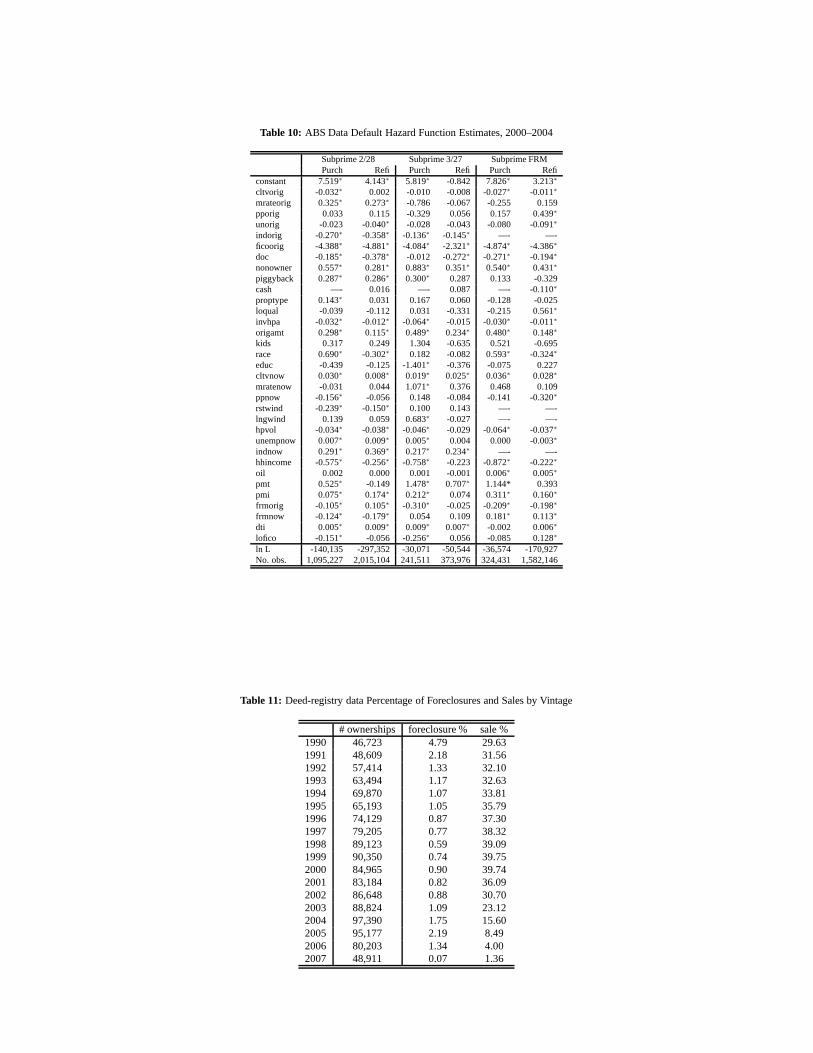
Table 10: ABS Data Default Hazard Function Estimates, 2000–2004

Subprime 2/28 Subprime 3/27 Subprime FRMPurch Refi Purch Refi Purch Refi

constant 7.519∗ 4.143∗ 5.819∗ -0.842 7.826∗ 3.213∗

cltvorig -0.032∗ 0.002 -0.010 -0.008 -0.027∗ -0.011∗

mrateorig 0.325∗ 0.273∗ -0.786 -0.067 -0.255 0.159pporig 0.033 0.115 -0.329 0.056 0.157 0.439∗

unorig -0.023 -0.040∗ -0.028 -0.043 -0.080 -0.091∗

indorig -0.270∗ -0.358∗ -0.136∗ -0.145∗ —- —-ficoorig -4.388∗ -4.881∗ -4.084∗ -2.321∗ -4.874∗ -4.386∗

doc -0.185∗ -0.378∗ -0.012 -0.272∗ -0.271∗ -0.194∗

nonowner 0.557∗ 0.281∗ 0.883∗ 0.351∗ 0.540∗ 0.431∗

piggyback 0.287∗ 0.286∗ 0.300∗ 0.287 0.133 -0.329cash —- 0.016 —- 0.087 —- -0.110∗

proptype 0.143∗ 0.031 0.167 0.060 -0.128 -0.025loqual -0.039 -0.112 0.031 -0.331 -0.215 0.561∗

invhpa -0.032∗ -0.012∗ -0.064∗ -0.015 -0.030∗ -0.011∗

origamt 0.298∗ 0.115∗ 0.489∗ 0.234∗ 0.480∗ 0.148∗

kids 0.317 0.249 1.304 -0.635 0.521 -0.695race 0.690∗ -0.302∗ 0.182 -0.082 0.593∗ -0.324∗

educ -0.439 -0.125 -1.401∗ -0.376 -0.075 0.227cltvnow 0.030∗ 0.008∗ 0.019∗ 0.025∗ 0.036∗ 0.028∗

mratenow -0.031 0.044 1.071∗ 0.376 0.468 0.109ppnow -0.156∗ -0.056 0.148 -0.084 -0.141 -0.320∗

rstwind -0.239∗ -0.150∗ 0.100 0.143 —- —-lngwind 0.139 0.059 0.683∗ -0.027 —- —-hpvol -0.034∗ -0.038∗ -0.046∗ -0.029 -0.064∗ -0.037∗

unempnow 0.007∗ 0.009∗ 0.005∗ 0.004 0.000 -0.003∗

indnow 0.291∗ 0.369∗ 0.217∗ 0.234∗ —- —-hhincome -0.575∗ -0.256∗ -0.758∗ -0.223 -0.872∗ -0.222∗

oil 0.002 0.000 0.001 -0.001 0.006∗ 0.005∗

pmt 0.525∗ -0.149 1.478∗ 0.707∗ 1.144* 0.393pmi 0.075∗ 0.174∗ 0.212∗ 0.074 0.311∗ 0.160∗

frmorig -0.105∗ 0.105∗ -0.310∗ -0.025 -0.209∗ -0.198∗

frmnow -0.124∗ -0.179∗ 0.054 0.109 0.181∗ 0.113∗

dti 0.005∗ 0.009∗ 0.009∗ 0.007∗ -0.002 0.006∗

lofico -0.151∗ -0.056 -0.256∗ 0.056 -0.085 0.128∗

ln L -140,135 -297,352 -30,071 -50,544 -36,574 -170,927No. obs. 1,095,227 2,015,104 241,511 373,976 324,431 1,582,146

Table 11: Deed-registry data Percentage of Foreclosures and Sales by Vintage

# ownerships foreclosure % sale %1990 46,723 4.79 29.631991 48,609 2.18 31.561992 57,414 1.33 32.101993 63,494 1.17 32.631994 69,870 1.07 33.811995 65,193 1.05 35.791996 74,129 0.87 37.301997 79,205 0.77 38.321998 89,123 0.59 39.091999 90,350 0.74 39.752000 84,965 0.90 39.742001 83,184 0.82 36.092002 86,648 0.88 30.702003 88,824 1.09 23.122004 97,390 1.75 15.602005 95,177 2.19 8.492006 80,203 1.34 4.002007 48,911 0.07 1.36

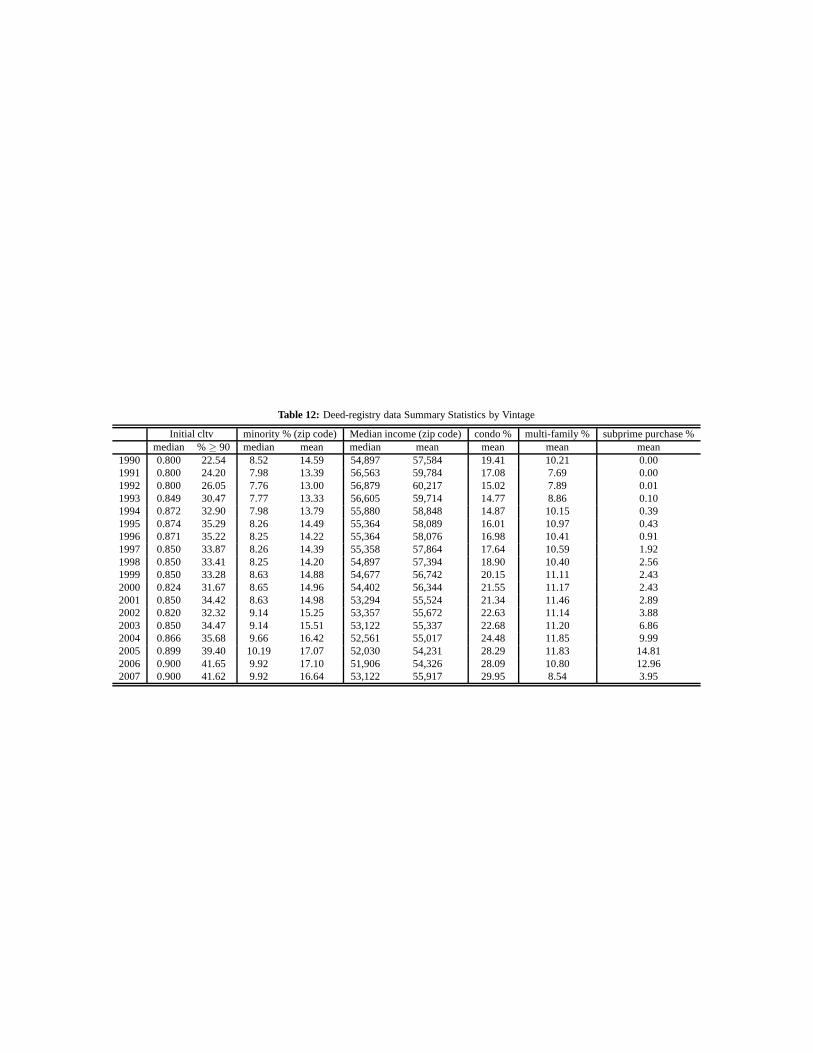
Table 12: Deed-registry data Summary Statistics by Vintage

Initial cltv minority % (zip code) Median income (zip code) condo % multi-family % subprime purchase %median %≥ 90 median mean median mean mean mean mean

1990 0.800 22.54 8.52 14.59 54,897 57,584 19.41 10.21 0.001991 0.800 24.20 7.98 13.39 56,563 59,784 17.08 7.69 0.001992 0.800 26.05 7.76 13.00 56,879 60,217 15.02 7.89 0.011993 0.849 30.47 7.77 13.33 56,605 59,714 14.77 8.86 0.101994 0.872 32.90 7.98 13.79 55,880 58,848 14.87 10.15 0.391995 0.874 35.29 8.26 14.49 55,364 58,089 16.01 10.97 0.431996 0.871 35.22 8.25 14.22 55,364 58,076 16.98 10.41 0.911997 0.850 33.87 8.26 14.39 55,358 57,864 17.64 10.59 1.921998 0.850 33.41 8.25 14.20 54,897 57,394 18.90 10.40 2.561999 0.850 33.28 8.63 14.88 54,677 56,742 20.15 11.11 2.432000 0.824 31.67 8.65 14.96 54,402 56,344 21.55 11.17 2.432001 0.850 34.42 8.63 14.98 53,294 55,524 21.34 11.46 2.892002 0.820 32.32 9.14 15.25 53,357 55,672 22.63 11.14 3.882003 0.850 34.47 9.14 15.51 53,122 55,337 22.68 11.20 6.862004 0.866 35.68 9.66 16.42 52,561 55,017 24.48 11.85 9.992005 0.899 39.40 10.19 17.07 52,030 54,231 28.29 11.83 14.812006 0.900 41.65 9.92 17.10 51,906 54,326 28.09 10.80 12.962007 0.900 41.62 9.92 16.64 53,122 55,917 29.95 8.54 3.95

Table 13: Massachusetts Subprime Lender Originations 1999–2007

Lender # total # purchase Lender # total # purchase Lender # total # purchaseoriginations originations originations originations originations originations

2007 2004 2001Summit 1,601 1,584 Option One 3,767 3,129 Option One 2,660 1,111Option One 360 358 New Century 2,991 2,507 New Century 1,263 323Equifirst 195 195 Freemont 2,895 2,461 Ameriquest 1,984 296New Century 149 149 Argent 2,200 2,068 Citifinancial Services 1,040 140Freemont 108 107 Fieldstone 1,131 1,023 Freemont 748 317Accredited Home 75 74 Accredited Home 1,014 820 Household Financial Corp. 548 61Argent 73 73 Mortgage Lender Net 972 536 Wells Fargo Finance 467 43Aegis 54 53 Nation One 946 927 Argent 457 66Wilmington Finance 46 43 WMC 888 586 First Franklin 367 251Nation One 44 44 Long Beach 812 685 Meritage 349 333Total 3,021 2,956 Total 23,761 18,481 Total 15,308 4,595

2006 2003 2000Mortgage Lender Net 2,489 2,310 Option One 3,157 2222 Option One 2,773 1,000Summit 2,021 1,948 New Century 1,694 1053 Ameriquest 2,047 287Freemont 2,016 1,973 Freemont 1,519 1089 Citifinancial Services 1,275 112New Century 1,978 1,942 Ameriquest 1,288 436 New Century 1,251 336WMC 1,888 1,860 First Franklin 922 917 Freemont 773 267Option One 1,616 1,552 Argent 836 536 Household Financial Corp. 761 55Accredited Home 1,006 986 Mortgage Lender Net 802 381 Long Beach 470 289Argent 640 626 Accredited Home 636 428 First Franklin 464 407Southstar 632 624 Fieldstone 585 430 Mortgage Lender Net 464 36Equifirst 598 564 Citifinancial Services 459 70 Argent 437 48Total 18,211 17,489 Total 17,988 11,062 Total 15,870 3,982

2005 2002 1999Option One 4,409 4,152 Option One 2,822 1502 Option One 2,828 1013Freemont 3,927 3,675 Ameriquest 1,713 526 Ameriquest 1,929 229New Century 3,125 2,906 New Century 1,261 443 Citifinancial Services 1,303 108Argent 2,253 2,195 Freemont 1,071 595 New Century 1,273 340WMC 1,846 1,681 First Franklin 657 622 Freemont 738 233Accredited Home 1,601 1,498 Citifinancial Services 656 97 Household Financial Corp. 728 47Long Beach 1,599 1,551 Mortgage Lender Net 627 170 Wells Fargo Finance 478 26Summit 1,588 1,440 Argent 606 166 Mortgage Lender Net 452 44Mortgage Lender Net 1,494 1,211 Wells Fargo Finance 411 27 Long Beach 413 202Nation One 969 959 Accredited Home 358 184 Argent 410 38Total 28,464 26,128 Total 15,296 6,459 Total 16,161 3,852

Table 14: Estimates of Foreclosure Hazard Using deed-registry data

1990–2007 Sample 1990–2004 Sample 2000–2004 SampleCoef Std. Err. Coef Std. Err. Coef Std. Err.

initial LTV -0.27 0.19 -1.40 0.22 -0.82 1.71LIBOR (6-month) 1.96e−02 1.39e−02 -3.09e−02 1.52e−02 0.18 0.11unemployment rate 4.74e−02 6.00e−03 5.03e−02 6.14e−03 7.70e−02 5.24e−03

% minority (2000 zip-code) 9.23e−03 1.03e−03 1.09e−02 1.20e−03 6.30e−03 4.31e−03

median income (2000 zip-code)-1.60e−05 1.82e−06 -1.71e−05 2.05e−06 -6.90e−05 1.03e−05

condo indicator 0.33 0.05 0.44 0.05 -1.19 0.35multi-family property indicator 0.54 0.05 0.54 0.06 -0.24 0.20subprime purchase indicator 1.99 0.06 1.21 0.19 1.70 0.21# observations 3,005,137 2,365,999 813,802

Table 15: The outcomes of S&P RMBS ratings, 1978–2004. From “Rating Transitions 2004: U.S. RMBS Stellar Performance Continues to Set Records,”Standard and Poor’s, January 21, 2005.

# rated Upgrade Downgrade DefaultAAA 6,137 – 0.5 0.07AA 5,702 22.4 3.6 0.5A 4,325 16.2 1.3 0.7BBB 4,826 11.1 2.0 1.2BB 2,042 17.9 2.3 1.4B 1,687 14.1 4.1 3.1

Table 16: Standardized Elasticities from Estimates Using deed-registry data

1990–2007 1990–2004 2000–2004(+/-) std. dev. factor change factor change factor change

in hazard in hazard in hazardUnemployment rate (+) 2.06 1.10 1.12 1.17% minority (2000 zip-code) (+) 19.58 1.20 1.24 1.13Median income (2000 zip-code) (−) $24,493 1.49 1.53 5.60Multi-family indicator . 1.72 1.72 0.79Condo indicator . 1.39 1.55 0.30Subprime purchase indicator . 7.32 3.35 5.47

Figure 1: Twelve-Month Default Rate on Subprime Mortgages

1999 2001 2003 2005 20070

5

10

15

20

25

30

Origination date

Per

cent

of l

oans

NOTE. Figure shows the percent of loans that default within 12 months of origination, by month of origination, from Jan.1999 to Dec. 2006, from the ABS data.

Figure 2: FICO Distribution of Subprime Mortgage Borrowers

1999 2001 2003 2005 20070

20

40

60

80

100

Date

Per

cent

FICO≥ 680620≤ FICO<680FICO< 620

NOTE. Figure shows distribution of subprime loans by credit score at origination, by month, from January 1999 to Decem-ber 2007, from the ABS data.

Figure 3: Evolving Underwriting Characteristics on Subprime Mortgages. Source: LP ABS data.

% Low Documentation Leverage

1999 2001 2003 2005 20070

10

20

30

40

50

60

Date

Per

cent

1999 2001 2003 2005 20070

10

20

30

40

50

60

Date

Per

cent

High LTVWith second lien

Other Subprime Mortgage Risk Factors Risk Layering

1999 2001 2003 2005 20070

10

20

30

40

50

60

Date

Per

cent

Non−traditional amortizationNon−owner occupiedPurchase

1999 2001 2003 2005 20070

10

20

30

40

50

60

Date

Per

cent

High CLTV + Low FICOHigh CLTV + Low/no DocHigh CLTV + Purchase

Figure 4: Default Characteristics on Subprime Mortgages by Month of Origination. Source: LP ABS data.

1999 2001 2003 2005 20070

5

10

15

20

25

30

Origination date

Per

cent

of l

oans

Full documentationIncomplete documentation

1999 2001 2003 2005 20070

5

10

15

20

25

30

Origination date

Per

cent

of l

oans

CLTV≥ 90 percent (or second lien recorded)CLTV<90 percent (and no second lien recorded)

1999 2001 2003 2005 20070

5

10

15

20

25

30

Origination date

Per

cent

of l

oans

Non−owner occupiedOwner occupied

1999 2001 2003 2005 20070

5

10

15

20

25

30

Origination date

Per

cent

of l

oans

Loan Purpose: RefinanceLoan Purpose: All other

1999 2001 2003 2005 20070

5

10

15

20

25

30

Origination date

Per

cent

of l

oans

Non−traditional amortization scheduleTraditional amortization schedule

Figure 5: Twelve-Month Default Rates on Loans with Risk Layering

(a) FICO Scores

1999 2001 2003 2005 20070

5

10

15

20

25

30

Origination date

Per

cent

of l

oans

High LTV and low FICO scoreAll other loans

(b) Loan Purpose: Purchase vs. Refi

1999 2001 2003 2005 20070

5

10

15

20

25

30

Origination date

Per

cent

of l

oans

High LTV and loan purpose=purchaseAll other loans

(c) Documentation Status

1999 2001 2003 2005 20070

5

10

15

20

25

30

Origination date

Per

cent

of l

oans

High LTV and low/no docAll other loans

NOTE. Figure shows the percentage of loans that default within 12 months of origination conditional on three risk factors,by month of origination, from Jan. 1999 to Dec. 2006, from the ABS data. Panel (a) gives results by owner occupancy,panel (b) gives results by loan purpose, and panel (c) gives results for loans with non-traditional amortization schedules.

Figure 6: Effect of CLTV on Default and Interest Rate

(a) Default Probabilities

70 80 90 100 1100.03

0.04

0.05

0.06

0.07

0.08

CLTV at origination

Def

ault

prob

abili

ty

Model 1Model 2

(b) Initial Contract Interest Rates

70 80 90 100 1106.5

7.0

7.5

8.0

8.5

CLTV at origination

Initi

al c

ontr

act r

ate

(per

cent

)

Model 1Model 2

NOTE. Figure shows graphically the results of the models estimated in Table 3.

Figure 7: Vintage Simulations Using ABS Data

(a) Defaults

1 6 12 18 24 30 36 400

5

10

15

20

Loan age (months)

Per

cent

of l

oans

2004 vintage: Data2004 vintage: Simulation2005 vintage: Data2005 vintage: Simulation

(b) Prepayments

1 6 12 18 24 30 36 400

10

20

30

40

50

60

70

Loan age (months)

Per

cent

of l

oans

2004 vintage: Data2004 vintage: Simulation2005 vintage: Data2005 vintage: Simulation

NOTE. Figures show actual and simulated cumulative defaults (top panel) and prepayments (bottom panel) for the 2004and 2005 vintages of loans. The simulations assume perfect foresight about house prices, interest rates, oil prices, andunemployment rates.

Figure 8: Effect of House Prices on a Generic 2/28 in the ABS Data

(a) Defaults

1 6 12 18 240

0.2

0.4

0.6

0.8

1.0

1.2

1.4

Loan age (months)

Per

cent

2004−−2006 House prices2006−−2008 House prices

(b) Prepayments

1 6 12 18 240

5

10

15

20

Loan age (months)

Per

cent

2004−−2006 House prices2006−−2008 House prices

NOTE. Figures show the probability in montht of default (top panel) and prepayments, conditional on surviving to montht − 1 for a generic hybrid 2/28 subprime mortgage as described in Table 7; the dynamic variables follow their 2004 to2006 trajectories, except for house prices, which are set either to their 2004 to 2006 trajectories or to their 2006 to 2008trajectories. The model used to produce the estimates is described in the text.

Figure 9: Massachusetts House Prices and Foreclosure Rates, January 1990 to December 2007

80

100

120

140

160

180200220

0

0.2

0.4

0.6

0.8

87 88 89 90 91 92 93 94 95 96 97 98 99 00 01 02 03 04 05 06 07 08

%o

fho

me

sfo

recl

ose

d

Year

ւ Foreclosure rate

Ho

use

Price

Ind

ex,(19

87

Q1

=1

00

)

House price levelց

ւ Cyclical Peak, Q3, 1988

The foreclosure rate is calculated at a quarterly frequency. The numerator is the total number of foreclosuresin MA in a given quarter and is obtained directly from the Warren Group data. The denominator is thenumber of residential parcels in a given year, where a parcel is defined as a real unit of property used forthe assessment of property taxes, and a typical parcel consists of a plot of land defined by a deed and anybuildings located on the land. Information on parcel counts is obtained from the Massachusetts Departmentof Revenue. Finally, house prices are calculated using the Case-Shiller weighted, repeat-sales methodology,using data from the Warren Group.

Figure 10: Estimate of Baseline Hazards

1 2 3 4 5 6 70

0.02

0.04

0.06

0.08

0.1

0.12

0.14

0.16

0.18

Years since House Purchase

Con

ditio

nal P

roba

bilit

y of

Def

ault

(%)

Foreclosure

1 2 3 4 5 6 7 80.4

0.45

0.5

0.55

0.6

0.65

0.7

0.75

0.8

0.85

0.9

Years since House Purchase

Con

ditio

nal S

ale

Rat

e (%

)

Sale

Figure 11: Estimated Effect of Equity on Foreclosure

−50 −25 0 25 50 75 100 125 1500

0.2

0.4

0.6

0.8

1

1.2

1.4

1.6

1.8

2

2.2

2.41990–2007 Data

Fo

recl

osu

reR

ate

(%)

Equity (%)−50 −25 0 25 50 75 100 125 1500

0.2

0.4

0.6

0.8

1

1.2

1.4

1.6

1.8

2

2.2

2.41990–2004 Data

Fo

recl

osu

reR

ate

(%)

Equity (%)

−50 −25 0 25 50 75 100 125 1500

0.2

0.4

0.6

0.8

1

1.2

1.4

1.6

1.8

2

2.2

2.42000–2004 Data

Fo

recl

osu

reR

ate

(%)

Equity (%)

Figure 12: 2004 Subprime Purchase Vintage Simulations

1 2 3 40

1

2

3

4

5

6

7

8

9

10

11

12

(2005:Q1) (2006:Q1) (2007:Q1)

← actual

predicted →

1990–2007 (In-Sample Fit)

Cu

m.

Fo

recl

osu

res

(%)

1 2 3 40

1

2

3

4

5

6

7

8

9

10

(2005:Q1) (2006:Q1) (2007:Q1)

1990–2004 (Out-of-Sample Fit)

Cu

m.

Fo

recl

osu

res

(%)

1 2 3 40

1

2

3

4

5

6

7

8

9

10

(2005:Q1) (2006:Q1) (2007:Q1)

2000–2004 (Out-of-Sample Fit)

Cu

m.

Fo

recl

osu

res

(%)

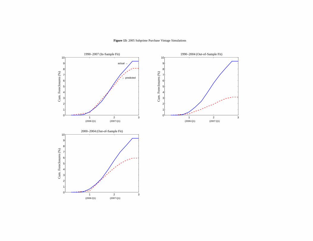
Figure 13: 2005 Subprime Purchase Vintage Simulations

1 2 30

1

2

3

4

5

6

7

8

9

10

(2006:Q1) (2007:Q1)

← predicted

actual →

1990–2007 (In-Sample Fit)

Cu

m.

Fo

recl

osu

res

(%)

1 2 30

1

2

3

4

5

6

7

8

9

10

(2006:Q1) (2007:Q1)

1990–2004 (Out-of-Sample Fit)

Cu

m.

Fo

recl

osu

res

(%)

1 2 30

1

2

3

4

5

6

7

8

9

10

(2006:Q1) (2007:Q1)

2000–2004 (Out-of-Sample Fit)

Cu

m.

Fo

recl

osu

res

(%)

Figure 14: HPA and the Cost of Insuring Subprime-backed Securities. Source: Haver Analytics and Markit.

_

−30

−20

−10

10

20

40

60

80

100

0

0

HP

Ain

%,S

AA

R

S&P Case-Shiller 20-cityր

2006 2007 2008

Q1Q1Q1 Q2Q2Q2 Q3Q3Q3 Q4Q4

AB

X(i

nve

rte

dsc

ale

)

տABX-HE, 06-01-AAA

ABX-HE, 06-01-BBB→

Figure 15: Bank C’s 2006 Estimated Relationship between HPA and Delinquency and Cumulative Losses. Source: Bank C.

Delinquency Rates

−40 −20

30

40

40

50

60

0

0

10

20

20

%o

fori

gin

alb

ala

nce

Cumulative HPA in %

ւIn-Sample

ւOut-of-Sample

Cumulative Losses after two years

−40 −20 40 60−1

0

0

1

2

3

4

5

6

7

8

20

%o

fori

gin

alb

ala

nce

Cumulative HPA in %

ւIn-Sample

ւOut-of-Sample

74