IMPERIAL COLLEGE LONDON

DEPARTMENT OF COMPUTING

Making Faster FEM Solvers, FasterMPhil Transfer Report

By

Graham Markall

Supervisors: Prof. Paul Kelly and Dr. David Ham

June 2010

Abstract

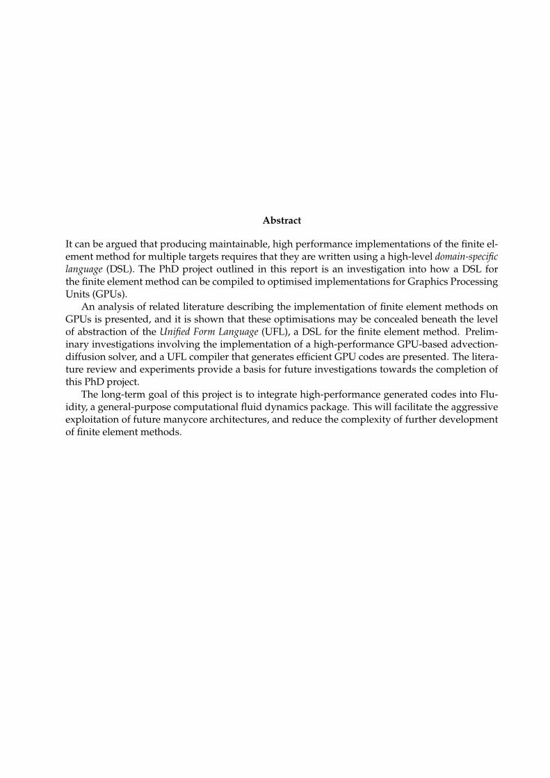
It can be argued that producing maintainable, high performance implementations of the finite el-ement method for multiple targets requires that they are written using a high-level domain-specificlanguage (DSL). The PhD project outlined in this report is an investigation into how a DSL forthe finite element method can be compiled to optimised implementations for Graphics ProcessingUnits (GPUs).

An analysis of related literature describing the implementation of finite element methods onGPUs is presented, and it is shown that these optimisations may be concealed beneath the levelof abstraction of the Unified Form Language (UFL), a DSL for the finite element method. Prelim-inary investigations involving the implementation of a high-performance GPU-based advection-diffusion solver, and a UFL compiler that generates efficient GPU codes are presented. The litera-ture review and experiments provide a basis for future investigations towards the completion ofthis PhD project.

The long-term goal of this project is to integrate high-performance generated codes into Flu-idity, a general-purpose computational fluid dynamics package. This will facilitate the aggressiveexploitation of future manycore architectures, and reduce the complexity of further developmentof finite element methods.

Contents

1 Introduction 11.1 Motivation and Outline . . . . . . . . . . . . . . . . . . . . . . . . . . . . . . . . . . . 11.2 Publications and Presentations . . . . . . . . . . . . . . . . . . . . . . . . . . . . . . . 21.3 Report Structure . . . . . . . . . . . . . . . . . . . . . . . . . . . . . . . . . . . . . . . . 2

2 Background 32.1 Introduction . . . . . . . . . . . . . . . . . . . . . . . . . . . . . . . . . . . . . . . . . . 32.2 Manycore Architectures . . . . . . . . . . . . . . . . . . . . . . . . . . . . . . . . . . . 3

2.2.1 Current Hardware - NVidia Fermi . . . . . . . . . . . . . . . . . . . . . . . . . 32.2.2 Performance Considerations . . . . . . . . . . . . . . . . . . . . . . . . . . . . 52.2.3 Other Architectures . . . . . . . . . . . . . . . . . . . . . . . . . . . . . . . . . . 52.2.4 Programming Languages . . . . . . . . . . . . . . . . . . . . . . . . . . . . . . 52.2.5 Remarks . . . . . . . . . . . . . . . . . . . . . . . . . . . . . . . . . . . . . . . . 6

2.3 The Finite Element Method . . . . . . . . . . . . . . . . . . . . . . . . . . . . . . . . . 72.3.1 A Brief Overview . . . . . . . . . . . . . . . . . . . . . . . . . . . . . . . . . . . 72.3.2 Boundary Conditions . . . . . . . . . . . . . . . . . . . . . . . . . . . . . . . . 8

2.4 Implementation . . . . . . . . . . . . . . . . . . . . . . . . . . . . . . . . . . . . . . . . 82.5 Conclusions . . . . . . . . . . . . . . . . . . . . . . . . . . . . . . . . . . . . . . . . . . 10

3 Literature Review 113.1 Introduction . . . . . . . . . . . . . . . . . . . . . . . . . . . . . . . . . . . . . . . . . . 113.2 The FEniCS Project and UFL . . . . . . . . . . . . . . . . . . . . . . . . . . . . . . . . . 11

3.2.1 UFL Compiler Optimisations . . . . . . . . . . . . . . . . . . . . . . . . . . . . 123.3 The Implementation of the Finite Element Method on GPUs . . . . . . . . . . . . . . 13

3.3.1 Data Layout and Alignment . . . . . . . . . . . . . . . . . . . . . . . . . . . . . 133.3.2 Mesh Reordering . . . . . . . . . . . . . . . . . . . . . . . . . . . . . . . . . . . 143.3.3 Kernel Granularity and Kernel Fusions . . . . . . . . . . . . . . . . . . . . . . 14

3.4 Colouring and Partitioning . . . . . . . . . . . . . . . . . . . . . . . . . . . . . . . . . 163.4.1 Oplus2 . . . . . . . . . . . . . . . . . . . . . . . . . . . . . . . . . . . . . . . . . 17

3.5 Algebraic Transformations . . . . . . . . . . . . . . . . . . . . . . . . . . . . . . . . . . 173.5.1 Transforming the Global Assembly Phase . . . . . . . . . . . . . . . . . . . . . 173.5.2 Evaluation of Integral Forms by Tensor Representation . . . . . . . . . . . . . 18

3.6 Related Areas . . . . . . . . . . . . . . . . . . . . . . . . . . . . . . . . . . . . . . . . . 193.6.1 Library Generators . . . . . . . . . . . . . . . . . . . . . . . . . . . . . . . . . . 193.6.2 Acumen . . . . . . . . . . . . . . . . . . . . . . . . . . . . . . . . . . . . . . . . 213.6.3 Autotuning Libraries . . . . . . . . . . . . . . . . . . . . . . . . . . . . . . . . . 213.6.4 Active Libraries . . . . . . . . . . . . . . . . . . . . . . . . . . . . . . . . . . . . 223.6.5 Formal Linear Algebra Methods Environment . . . . . . . . . . . . . . . . . . 22

3.7 Conclusions . . . . . . . . . . . . . . . . . . . . . . . . . . . . . . . . . . . . . . . . . . 22

i

4 Preliminary Investigations 254.1 Introduction . . . . . . . . . . . . . . . . . . . . . . . . . . . . . . . . . . . . . . . . . . 254.2 Data Format Considerations . . . . . . . . . . . . . . . . . . . . . . . . . . . . . . . . . 254.3 Experiments . . . . . . . . . . . . . . . . . . . . . . . . . . . . . . . . . . . . . . . . . . 26

4.3.1 CUDA and CPU Implementations and Experimental Setup . . . . . . . . . . 264.3.2 Results . . . . . . . . . . . . . . . . . . . . . . . . . . . . . . . . . . . . . . . . . 27

4.4 Further Investigations . . . . . . . . . . . . . . . . . . . . . . . . . . . . . . . . . . . . 294.5 A Prototype Compiler . . . . . . . . . . . . . . . . . . . . . . . . . . . . . . . . . . . . 29

4.5.1 Further UFL Compiler Development . . . . . . . . . . . . . . . . . . . . . . . . 294.6 Conclusions . . . . . . . . . . . . . . . . . . . . . . . . . . . . . . . . . . . . . . . . . . 30

5 Research Plan 335.1 Introduction . . . . . . . . . . . . . . . . . . . . . . . . . . . . . . . . . . . . . . . . . . 335.2 Work Items . . . . . . . . . . . . . . . . . . . . . . . . . . . . . . . . . . . . . . . . . . . 335.3 Potential Publications . . . . . . . . . . . . . . . . . . . . . . . . . . . . . . . . . . . . . 355.4 Conclusions . . . . . . . . . . . . . . . . . . . . . . . . . . . . . . . . . . . . . . . . . . 36

ii

Chapter 1

Introduction

This report describes a summary of the research that has been completed during the first 9 monthsof my PhD. This research forms a basis for further study over the next two years.

1.1 Motivation and Outline

Fluidity [Gorman et al., 2009, Piggott et al., 2009] is a computational fluid dynamics package thatuses the finite element method on unstructured meshes to simulate complex models of oceans andother phenomena. It is composed of hundreds of thousands of lines of Fortran code.

The recent emergence of manycore architectures (including GPUs) as platforms that offer alarge increase in computational power over traditional architectures motivates their exploitationfor computational science applications. In order to make use of these architectures with Fluidity,portions of the code must be rewritten using CUDA or OpenCL, which are the languages cur-rently available for programming these devices. However, this will require a large investmentin time and effort. Additionally, the rewritten code must be tuned for each new architecture. Itis also unlikely that CUDA and OpenCL will remain the languages of choice for programmingfuture architectures; when they are replaced, it will again be necessary to rewrite large portions ofFluidity.

We note that in general the development of finite element codes in low-level languages iscomplicated and error prone. This process is further complicated by the fact that optimal datalayouts and access patterns differ between targets, especially when execution of the code spansmultiple architectures. Additionally, the optimal choice of algorithm that implements a givenoperation depends on characteristics of the target hardware, and even the parameters of a specificproblem. To produce efficient implementations in a low-level language, developers must maintainmultiple algorithm implementations for multiple targets.

It can be argued that producing maintainable high-performance implementations of finite el-ement methods for multiple targets requires that they are written using a high-level domain-specific language. The Unified Form Language (UFL) [Alnæs and Logg, 2009], is one such high-levellanguage that allows the generation of high-performance code from maintainable sources.

This PhD project is an investigation into how tools that generate efficient low-level code forGPUs from high-level specifications written in UFL may be developed and integrated into existingcodebases. Part of this investigation involves determining how finite element assembly shouldbe implemented on GPUs in order to obtain high performance. The remainder of the projectinvolves building a UFL compiler and embedding into it the domain knowledge that enables itto generate these optimised implementations. The completion of this project will enable a largeportion of Fluidity to be rewritten in UFL, allowing future architectures to be targeted more easily,and reducing the complexity of software development.

1

1.2 Publications and Presentations

A number of presentations describing the work of this project have been given outside the college.These include:

• Experiments in unstructured mesh finite element CFD using CUDA [Markall et al., 2009].This presentation was given at the 1st UK CUDA Developers’ Conference, and won theprize for the best student presentation.

• Generating optimised multiplatform finite element solvers from high-level representations[Markall et al., 2010b]. This presentation was given at the 8th meeting of the IFIP WorkingGroup 2.11 on Program Generation.

• Experiments in generating and integrating GPU-accelerated finite element solvers using theUnified Form Language [Markall et al., 2010a]. This presentation was given at the FEniCS’10 Conference.

The work already completed has also been published:

• Towards generating optimised finite element solvers for GPUs from high-level specifica-tions [Markall et al., 2010c]. This publication was presented at the workshop on AutomatedProgram Generation for Computational Science1 at the 10th International Conference onComputational Science.

1.3 Report Structure

We begin by providing background information about GPU architectures and the finite elementmethod in Chapter 2. We examine the literature discussing the implementation of finite elementmethods on GPUs, and automated programming of the finite element method in Chapter 3. Prac-tical investigations that have been completed are reported in Chapter 4. A plan for the proposedresearch is outlined in Chapter 5.

1http://www.sc.rwth-aachen.de/Events/APGCSatICCS2010/

2

Chapter 2

Background

2.1 Introduction

We begin by discussing manycore architectures, in particular the NVidia Fermi architecture. Thisdiscussion serves to highlight the differences in programming each architecture, and to draw at-tention to the challenges that must be overcome, particularly when implementing computationsthat use unstructured data.

Subsequently, we introduce the finite element method and discuss how it is typically imple-mented on CPU architectures. This is used as a foundation to our discussions of the variousimplementation choices that may be made on manycore architectures in the following chapters.

2.2 Manycore Architectures

2.2.1 Current Hardware - NVidia Fermi

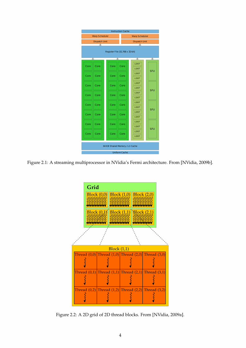
Graphics Processing Units (GPUs) are highly-parallel architectures that have a large memory band-width and many streaming multiprocessors (SMs). Figure 2.1 shows a schematic diagram of an SMin NVidia’s latest architecture, Fermi [NVidia, 2009a]. The SM may be thought of as similar to aSIMD execution unit, or a 32-lane vector processor.

There are several levels of the memory hierarchy in Fermi. We highlight the main levels thatrequire consideration when developing code for the Fermi architecture:

Global Memory. A Fermi card has up to 6GB of onboard memory that is accessible by all theSMs. This memory is the slowest, with a latency of hundreds of cycles. Since this memory isseparate from the memory of the host computer, data must be marshalled into this memorybefore computation on the GPU can begin.

L1 Caches. Each SM has 64KB of private cache. This cache is split into a 48KB portion and a 16KBportion. One of these portions may be assigned to a hardware-controlled cache and the otheris assigned to a software-controlled cache, at the choice of the programmer. The caches canbe accessed more quickly than global memory, although it has a limited number of banks,which can lead to conflicts that lower performance.

Registers. Each SM has 32,768 32-bit registers. These may be accessed very quickly. However,these registers are shared between potentially thousands of threads, leaving only a smallnumber per thread.

Execution on Fermi is performed by launching individual kernels that are executed by manythreads in parallel. These threads are grouped at various granularities, as shown in Figure 2.2. Thefinest grouping is referred to as a warp, made up of 32 threads that all share a program counter.Since these threads share a program counter, they execute in lock-step performing the same oper-ations on individual items of data.

3

Dispatch Unit

Warp Scheduler

Instruction Cache

Dispatch Unit

Warp Scheduler

Core

Core Core

Core Core

Core Core

Core Core

Core Core

Core Core

Core Core

Core Core

Core Core

Core Core

Core Core

Core Core

Core Core

Core Core

Core Core

SFU

SFU

SFU

SFU

LD/ST

LD/ST

LD/ST

LD/ST

LD/ST

LD/ST

LD/ST

LD/ST

LD/ST

LD/ST

LD/ST

LD/ST

LD/ST

LD/ST

LD/ST

LD/ST

64 KB Shared Memory / L1 Cache

Uniform Cache

Core

Register File (32,768 x 32-bit)

Figure 2.1: A streaming multiprocessor in NVidia’s Fermi architecture. From [NVidia, 2009b].

Grid

Block (0,0) Block (1,0) Block (2,0)

Block (0,1) Block (1,1) Block (2,1)

Block (1,1)

Thread (0,0) Thread (1,0) Thread (2,0) Thread (3,0)

Thread (0,1) Thread (1,1) Thread (2,1) Thread (3,1)

Thread (0,2) Thread (1,2) Thread (2,2) Thread (3,2)

Figure 2.2: A 2D grid of 2D thread blocks. From [NVidia, 2009a].

4

Several warps are grouped together to form a block, and the set of all blocks executing concur-rently makes up the grid. Individual SMs are assigned a number of blocks to execute. Becauseeach block has an affinity for one SM, communication between threads in different blocks is notpossible.

2.2.2 Performance Considerations

Since global memory is separate from the host’s memory, it is important to ensure that all com-putation within an inner loop is performed on the GPU. If the computation in the inner loop isdivided between the GPU and the host, execution speed will be greatly reduced due to the needto constantly transfer data across the PCIe bus.

Secondly, since warps all share a single program counter, and execute the same code path con-currently, it is important that they all follow the same path of execution in the code. When threadswithin a warp take different paths, execution is serialised between these two paths, reducing per-formance.

Finally, coalesced memory access is needed for high memory bandwidth utilisation, and isachieved when groups of 16 threads (half of a warp) concurrently access data within a 64-bytealigned memory window. Coalescing increases the memory bandwidth utilisation because it al-lows multiple accesses to be transferred across the very wide data bus in a single operation. Sincethe threads in a half-warp are all executing the same instruction, their accesses will occur at thesame time; when these accesses occur, the hardware can recognise that they fit within the windowand amalgamate the accesses into a single transfer.

We have discussed the main performance considerations when writing code for the Fermiarchitecture. There are other considerations that are required to obtain optimum performancethat are described in [NVidia, 2009a]. Often it is necessary to use tools such as the CUDA profiler[NVidia, 2010] to understand the performance of code.

2.2.3 Other Architectures

Although our current focus is on the Fermi architecture, it is important to note that there areother multicore and manycore architectures that are currently in use and in development. TheFermi architecture was preceded by the G80 and G200 Tesla architectures from NVidia. Althoughall the NVidia architectures share a programming model, their performance characteristics differ,meaning that code must be individually tuned for best performance on each device.

Other GPU architectures include AMD’s Evergreen architecture [AMD, 2010], that has peakperformance somewhere between that of the G200 and Fermi architectures. The Cell Proces-sor [Gschwind et al., 2006] is an interesting research platform due to its heterogeneous architec-tures, although it is not under further development. Intel’s forthcoming Larrabee architecture[Seiler et al., 2008] is heavily based on the x86 processor, and can be expected to have very differ-ent performance characteristics to GPU architectures.

2.2.4 Programming Languages

In order to make effective use of the GPU, programs must be designed such that the workloadis decomposed into many (thousands) of data-parallel tasks that can be mapped to individualthreads.

CUDA [NVidia, 2009a] is a language for programming NVidia’s Tesla Graphics Processing Units(GPUs). It is a set of extensions to the C programming language that allows the user to definekernels for execution on the device, and includes additional keywords that are used for managingthe execution of threads.

In order to give a brief overview of a CUDA kernel, we consider an example of a kernel thatperforms the computation y = αx + y for scalar α and vectors x and y. A C implementation ofthis operation uses a loop that iterates over each element in the vectors.

5

void daxpy(double a, double *x, double *y, int n)

for(int i=0; i<n; i++)

y[i] = y[i] + a*x[i];

Figure 2.3: DAXPY Kernel in C.

In order to convert this to a CUDA kernel, the work is divided between threads so that onethread computes the result for each element. This kernel is designed to be launched with as manythreads as there are vector elements. Each thread calculates the offset for the element that it isassigned from the ID of its thread block, and its own ID within the block.

__global__ void daxpy(double a, double *x, double *y, int n)

int i=threadIdx.x+blockIdx.x*blockDim.x;

if(i<n)

y[i] = y[i] + a*x[i];

Figure 2.4: DAXPY Kernel in CUDA.

In order to standardise development for multicore architectures, the OpenCL specification[Khronos Group, 2008] has been developed. The OpenCL language shares many of the featuresof CUDA. However, it is designed to be compiled to executable code for a wide range of archi-tectures, including GPUs, multicore CPUs, and the Cell processor. Since it is designed to be moreflexible than CUDA in terms of supported targets, the assumptions about grids and blocks thatare part of CUDA are abstracted away in OpenCL kernel code. Figure 2.5 gives an example of thedaxpy kernel in OpenCL.

__kernel void daxpy(const double a, __global const double *x,

__global double* y, int n)

int i = get_global_id(0);

if (i >= n)

return;

y[i] = y[i] + a*x[i];

Figure 2.5: DAXPY Kernel in OpenCL.

2.2.5 Remarks

Although it is easy to begin developing codes for GPUs and multicore systems, optimising theperformance of codes on these architectures is non-trivial. It is often the case that the optimaldivision of work between threads and the granularity of kernels is not obvious, and various ex-periments must be performed in search of an optimum. Each time a new GPU architecture isreleased, existing codes must be re-optimised, requiring a large investment of time and effort.

Although OpenCL is portable across many targets, it is not performance portable; in the sameway that different GPUs require the code to be optimised in different ways, optimising for differ-ent architectures requires further changes. Obtaining optimal performance from all the differentarchitectures a code may be run on is not sustainable as it will require constant development effort.

Additionally, managing the marshalling of data to and from the devices, and between thevarious levels of the memory hierarchy places further burden on the programmer. For example,making full use of the L1 caches on Fermi requires code to be written that explicitly marshals data

6

at the beginning and end of execution of each kernel. Since the characteristics of the caches canvary between architectures, this adds another dimension of complexity in maintaining code formultiple targets.

2.3 The Finite Element Method

2.3.1 A Brief Overview

The finite element method is used for discretising the weak form of partial differential equations.Here we provide a brief overview of the mathematical formulation of the method - for a full treat-ment, see [Karniadakis and Sherwin, 1999]. We will use this explanation as a base for describingthe implementation choices that may be made. The general formulation of an equation that maybe discretised using the finite element method is of the form:

L(u) = q (2.1)

where L is any linear differential operator, u is an independent variable, and q is a known functionthat does not depend on u. For example, L ≡ ∇2 and q is the source term in Poisson’s equation.Solving this equation numerically provides gives a solution uδ, which may not satisfy Equation2.1 perfectly. So we have:

R(uδ) = L(uδ)− q (2.2)

Here R is the residual, which provides a measure of the amount by which the numerical solu-tion does not satisfy the original problem. In the ideal case, R = 0, and the numerical solutionis the exact solution, so we must try to eliminate this term. However, requiring the numericalsolution to be exact makes it too difficult to find a solution to most problems. If we are preparedto tolerate some inaccuracy, we can transform the system to weaken the definition of equality.First, we multiply the equation by an arbitrary test function, v, and then integrate over the wholedomain, Ω, giving: ∫

ΩvR(uδ) dX =

∫Ω

vL(uδ) dX−∫

Ωvq dX (2.3)

Now, we assume that R = 0, which makes the integral on the left-hand side disappear, leaving uswith: ∫

ΩvL(uδ) dX =

∫Ω

vq dX (2.4)

This form is known as the integral form of Equation 2.1. The left-hand side of this equation definesan inner product between the test function v and the trial function L, and therefore can be consid-ered as a projection of v into L. Because the function q is known, we can evaluate the right-handside, and then compute the aforementioned projection to give uδ. This projection is known as theGalerkin Projection.

In order to evaluate the right-hand side and the projection at discrete points (as is necessary ona computer with finite memory and processing power), the integral form must be discretised. Thediscretisation allows us to represent functions in the test and trial spaces as a linear combination ofbasis functions. For example, we represent the solution as uδ = ∑N

i=1 uiΦi where N is the numberof functions in the basis for this space, and ui is the i-th coefficient of the i-th basis function, Φi.The basis functions are chosen so that

Φi(xi) = 1, and ∀k : i 6= k, Φi(xk) = 0 (2.5)

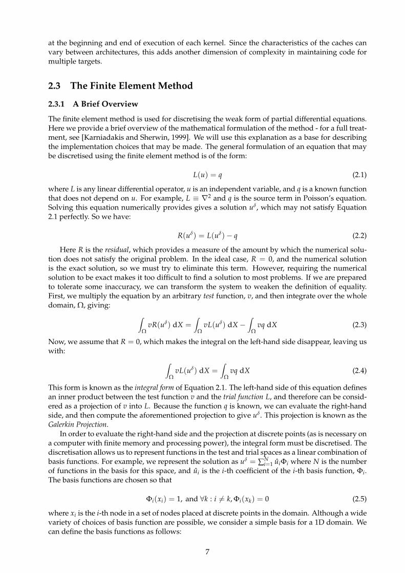
where xi is the i-th node in a set of nodes placed at discrete points in the domain. Although a widevariety of choices of basis function are possible, we consider a simple basis for a 1D domain. Wecan define the basis functions as follows:

7

1 2 3 4 1 2 3 4

1 2 3 4 1 2 3 4

Figure 2.6: A piecewise continuous linear basis over a one-dimensional domain with four nodesand three elements.

Φi =

x−xk−1xk−xk−1

if x ∈ [xk−1, xk]xk+1−xxk+1−xk

if x ∈ [xk, xk+1]

0 otherwise.

(2.6)

This is a piecewise linear basis. An example of this basis for a four-node domain is shown inFigure 2.6

Having decided on a discretisation, we may now proceed to evaluate the integrals on bothsides of Equation 2.4. The result of this process, a linear system of equations

Ax = b (2.7)

is assembled, in which the matrix A is derived from the LHS and the vector b is derived from theRHS of the weak form. The solution to this system of equations, x, is the solution to the discretisedproblem.

2.3.2 Boundary Conditions

Often boundary conditions must be enforced in order for there to a be a unique solution to adifferential equation. Boundary conditions are usually one of two kinds:

Dirichlet. These specify the exact value of a function at a boundary node. An example of a Dirich-let boundary condition is the no-slip condition, u = 0, which states that the velocity of a fluidis zero at a boundary, and the free-slip condition, u · n = 0, which states that fluid movesfreely along a boundary, but not through it.

Neumann. These specify the value of the derivative of a function at a boundary node. An exam-ple of a Neumann boundary condition is the do-nothing boundary condition, ∂u

∂X = 0, whichprescribes free flow out of the domain.

The implementation of boundary conditions in the finite element method involves a similarprocess to that for the entire domain. In evaluating boundary condition contributions, only theedges of the domain are considered, which requires computations in a domain of dimension thatis one lower than the whole domain. For example, in a 2D domain, 1D line integrals are evaluatedover the boundaries, and in a 3D domain, 2D surface integrals are evaluated over the boundaries.

2.4 Implementation

Solving a partial differential equation with a time-varying solution using the finite element methodtypically consists of the following phases for each timestep:

Local Assembly. For each element i in the domain, an Ne × Ne matrix, Mei , and an Ne-length vec-

tor, bei , are computed, where Ne is the number of nodes per element. These are referred to as

8

Ω1 Ω2 Ω1 Ω2

1 2 3 1 2 1 2

Figure 2.7: Left: A 1D domain decomposed into two elements (Ωi). Right: Local node numberingof individual elements.

local matrices and vectors. Computing these matrices and vectors usually involves the eval-uation of integrals over the elements using Gaussian quadrature. In most implementations,every element has the same number of nodes.

Global Assembly. The local matrices, Mei , and vectors, be

i , are used to form a global matrix, M, andglobal vector, b, respectively. This process couples the contributions of elements together.

Solution. The system of equations Mx = b is solved for x, often using an iterative method, whichrequires computation of the sparse matrix-vector product (SpMV) y = Mv.

We shall examine the global assembly phase, which consists of performing the following compu-tations:

M = ATMeA (2.8)

b = ATbe (2.9)

whereA is a matrix mapping the local node numbers of each element to the global node numbers,Me is a block-diagonal matrix whose i-th block is Me

i , and be is a vector of stacked bei . We shall

examine algorithms that can be used to implement these computations, as the optimal choice ofalgorithm depends on the target hardware. Consider a two-element, three-node decomposition ofa 1-dimensional domain (see Figure 2.7). In this example, the matrices and vector are:

A =

1

11

1

Me =

m1

11 m112

m121 m1

22m2

11 m212

m221 m2

22

be =

b1

1b1

2b2

1b2

2

where me

ij is the i, j-th term of the local matrix for element Ωe, and bei is the i-th term of the local

vector for element Ωe. The structure ofA arises from the geometry of the elemental decompositionof the domain.

It is often inefficient to compute the matrix multiplications described in Equations 2.8 and 2.9on traditional architectures due to the sparsity ofA. The Addto algorithm is usually more efficient.To describe this algorithm, we first define an array, map[e][i], that maps the local node i of theelement e to a global node number. In our example, the array is defined as:

map[1][i] =[

12

]map[2][i] =

[23

]Algorithms 1 and 2 describe the Addto algorithm for computing M and b. Intuitively, terms of thelocal matrix (or vector) of each element are summed into particular terms in the global matrix (orvector) depending on the node numbers of the element.

These algorithms are massively data-parallel, as iterations of all the loops can be executedindependently of others. Although this appears to make them ideal for implementing on GPUarchitectures, there are two issues. First, data races occur if threads concurrently update the sameterm of the global matrix. Costly atomic operations must be used to ensure correctness. Second, Mis often stored using a format such as compressed sparse row (CSR). Finding the location in memoryof a particular term requires a bisection search of the sparsity structure of the matrix, leading touncoalesced accesses and control flow divergence within warps.

9

Algorithm 1: Addto for global matrix assembly.

M = 0 ;1

foreach Element e do2

for i← 1 to Ne do3

for j← 1 to Ne do4

M[map[e][i], map[e][j]]+=Me[i, j] ;5

Algorithm 2: Addto for global vector assembly.

b = 0 ;1

foreach Element e do2

for i← 1 to Ne do3

b[map[e][i]]+=be[i] ;4

2.5 Conclusions

We have examined the Fermi architecture, and briefly discussed other multicore and manycorearchitectures. These architectures bring considerable challenges when developing unstructuredcodes, particularly due to their requirements for accessing data in a structured fashion. Further-more, the need to marshal data onto and off the device and through the various levels of theirmemory hierarchy further complicates code, and reduces its portability.

The finite element method is typically implemented using unstructured data and indirect ac-cesses, which are unlikely to be efficient when implemented on manycore architectures. In thefollowing chapter, we will examine some of the techniques that have been used to overcome theseissues and improve performance.

10

Chapter 3

Literature Review

3.1 Introduction

As we have seen in the previous chapter, the implementation of finite element methods on many-core architectures is challenging. In this chapter we examine how these issues have been tackled inimplementations that are described in the literature. In particular we will examine data structures,partitioning of the data and the tasks between threads, and strategies for avoiding contention be-tween parallel threads.

We begin by discussing the FEniCS project, which has worked towards the automation ofthe finite element method. The outputs of the FEniCS project, in particular the Unified FormLanguage, provide an appropriate level of abstraction for the finite element method that makes iteasy to develop and maintain codes, and allows flexible choice in the low-level implementationand a choice of optimisations to be made. Presently the FEniCS project tools provide supportfor CPU architectures only. We discuss how this work may be further extended to support thegeneration of CUDA/OpenCL, using alternative data structures and algorithms that are moreefficient on manycore architectures.

We also examine alternative algorithms for implementing the finite element method, and dis-cuss the impact that this has had on the performance of simulations with varying parameters onCPU architectures. These algorithms can also be implemented on GPU architectures, but theirperformance can be expected to vary differently in relation to the problem parameters.

Finally, we examine techniques that have been successfully used to generate optimised codefrom high-level specifications in other areas of computational science. These domains include sig-nal processing, cyber-physical systems, and tensor contraction computations for quantum chem-istry. We discuss how these techniques may be applied in the generation of finite element solversfrom high-level specifications.

3.2 The FEniCS Project and UFL

There are a number of tools that are designed to make the implementation of finite element meth-ods easier. These include libraries such as deal.II [Bangerth et al., 2007], Diffpack [Langtangen, 2003],Sundance [Long, 2003], as well as the XFEM library [Bordas et al., 2007] for the extended finite ele-ment method [Moes et al., 1999]. Domain-specific languages such as Analysa [Bagheri and Scott, 2004], FreeFEM [Hecht et al., 2005], GetDP [Dular and Geuzaine, 2005] and Hedge [Klockner, 2010] havealso been developed.

We focus our discussion on the FEniCS project [Logg, 2007], as the tools from this projectprovide complete automation of the finite element method. The main environment, DOLFIN[Logg and Wells, 2010] is used to define and solve a Partial Differential Equation (PDE) problem,allowing specification of the PDE, boundary conditions, the mesh, and timestepping. The UnifiedForm Language is used for the specification of variational forms.

For a complete UFL reference, see [Alnæs and Logg, 2009]. We examine UFL with an exam-ple that shows how it can be used to describe the assembly and solution of a partial differential

11

equation. Poisson’s Equation, and a weak form are:

∇2u = f (3.1)∫Ω∇v · ∇u dX =

∫Ω

v f dX (3.2)

We assume the boundary condition∫

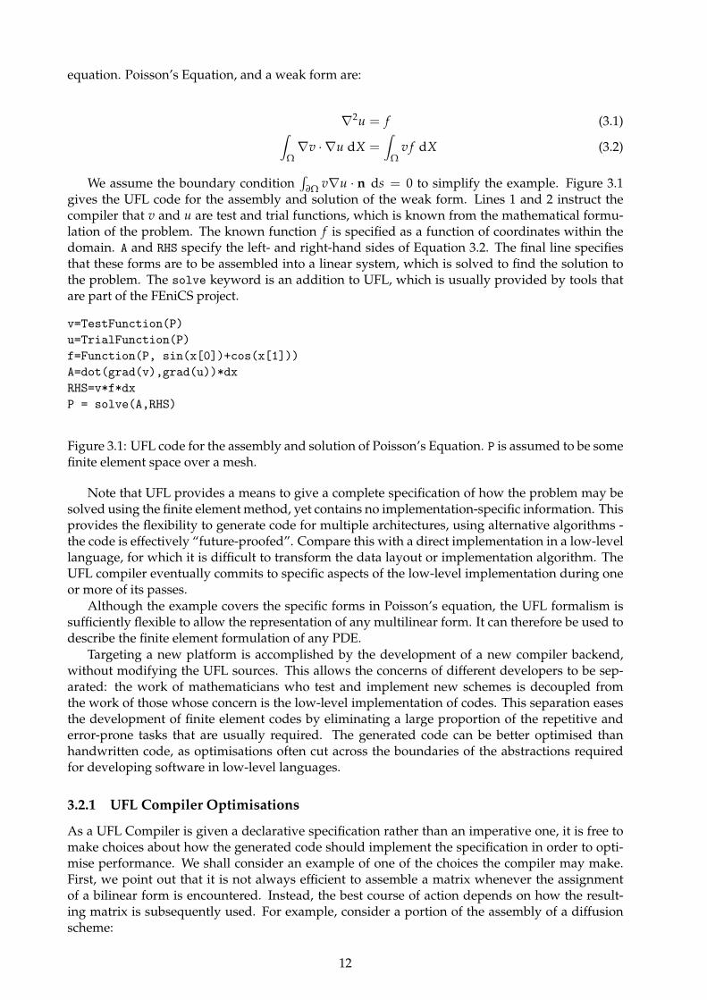
∂Ω v∇u · n ds = 0 to simplify the example. Figure 3.1gives the UFL code for the assembly and solution of the weak form. Lines 1 and 2 instruct thecompiler that v and u are test and trial functions, which is known from the mathematical formu-lation of the problem. The known function f is specified as a function of coordinates within thedomain. A and RHS specify the left- and right-hand sides of Equation 3.2. The final line specifiesthat these forms are to be assembled into a linear system, which is solved to find the solution tothe problem. The solve keyword is an addition to UFL, which is usually provided by tools thatare part of the FEniCS project.

v=TestFunction(P)

u=TrialFunction(P)

f=Function(P, sin(x[0])+cos(x[1]))

A=dot(grad(v),grad(u))*dx

RHS=v*f*dx

P = solve(A,RHS)

Figure 3.1: UFL code for the assembly and solution of Poisson’s Equation. P is assumed to be somefinite element space over a mesh.

Note that UFL provides a means to give a complete specification of how the problem may besolved using the finite element method, yet contains no implementation-specific information. Thisprovides the flexibility to generate code for multiple architectures, using alternative algorithms -the code is effectively “future-proofed”. Compare this with a direct implementation in a low-levellanguage, for which it is difficult to transform the data layout or implementation algorithm. TheUFL compiler eventually commits to specific aspects of the low-level implementation during oneor more of its passes.

Although the example covers the specific forms in Poisson’s equation, the UFL formalism issufficiently flexible to allow the representation of any multilinear form. It can therefore be used todescribe the finite element formulation of any PDE.

Targeting a new platform is accomplished by the development of a new compiler backend,without modifying the UFL sources. This allows the concerns of different developers to be sep-arated: the work of mathematicians who test and implement new schemes is decoupled fromthe work of those whose concern is the low-level implementation of codes. This separation easesthe development of finite element codes by eliminating a large proportion of the repetitive anderror-prone tasks that are usually required. The generated code can be better optimised thanhandwritten code, as optimisations often cut across the boundaries of the abstractions requiredfor developing software in low-level languages.

3.2.1 UFL Compiler Optimisations

As a UFL Compiler is given a declarative specification rather than an imperative one, it is free tomake choices about how the generated code should implement the specification in order to opti-mise performance. We shall consider an example of one of the choices the compiler may make.First, we point out that it is not always efficient to assemble a matrix whenever the assignmentof a bilinear form is encountered. Instead, the best course of action depends on how the result-ing matrix is subsequently used. For example, consider a portion of the assembly of a diffusionscheme:

12

M=p*q*dx # Mass matrix

rhs=action(M+0.5*d, t) # Right-hand side vector

A=M-0.5*d # Left-hand side matrix

In this example the mass matrix is not used as a matrix of coefficients in a system of equations,but is only used as an intermediary matrix for the construction of the matrix A, and the right-handside vector. Assembling a full sparse matrix for M will be very costly in terms of memory usage,and possibly in terms of computation required to construct the matrix sparsity pattern.

Since the mass matrix is not directly required, an efficient schedule for executing this codemay consist of fusing the loops that assemble the right-hand side vector and the matrix. After thisoptimisation, the local matrices that make up the mass matrix may be assembled for each elementin the mesh at each iteration of the loop - this local matrix may then be used to compute the actionof the mass matrix on the local vector, and also added into the local matrix for A. At the end of aniteration of the loop, the mass matrix is no longer required, and can be freed. To summarise theeffect of this optimisation, it avoids a Sparse Matrix-Vector (SpMV) product being computed for avery large sparse matrix, replacing it with many small, dense matrix-vector multiplications.

Whether it is more efficient to fully assemble the mass matrix or to only ever assemble itslocal matrices depends upon the target architecture. This example demonstrates that there is anoptimisation space to be explored, and that differs between architectures. Furthermore, the userof UFL need not consider this optimisation space as it is abstracted away.

There are further examples of optimisations that can be made without modifying the UFLsources. Other optimisations that we describe throughout the remainder of this chapter can beimplemented in a UFL compiler and effectively hidden from the end user. These optimisationsaffect aspects of the code including:

• The structure of the assembly loop. This structure determines the number of elements theloop operates on concurrently, how the kernels are fused.

• Changes to the layout of data structures representing the mesh and associated data, and itsalignment.

• Partitioning the computational workload and re-ordering of computations in order to avoidinefficient operations.

• The algorithms used to implement the global assembly phase.

3.3 The Implementation of the Finite Element Method on GPUs

There are a number of implementations of finite element methods on GPUs that are described inthe literature. These implementations have been applied to fields including earthquake modelling[Komatitsch et al., 2009, Komatitsch et al., 2010], electromagnetic scattering [Klockner et al., 2009,Klockner, 2010], hyperelastic material simulation [Filipovic et al., 2009a, Filipovic et al., 2010], andsurgical simulation [Miller et al., 2007, Taylor et al., 2007, Taylor et al., 2008, Comas et al., 2008]. In-vestigations into the implementation of the local assembly phase have shown that performanceon the GPU can vary between problems with various parameters [Maciol et al., 2010]. Some im-plementations of multigrid solvers on GPUs are used to accelerate the solution phase of the finiteelement method, including [Turek et al., 2010, Goddeke et al., 2009]. However, we exclude discus-sions of linear solvers from our review as they do not make up part of the finite element assemblyprocess. In the remainder of this section we examine the techniques used to implement the finiteelement method efficiently on GPU architectures.

3.3.1 Data Layout and Alignment

One approach [Klockner et al., 2009] described in the literature involves partitioning the mesh intosmall chunks that can be co-operatively loaded into shared memory by a thread block, before com-putation proceeds on this data. Since data is reused between elements that share a face, it is more

13

Element

Element

Element

Element

Element

Element

. . . . . . . . .

Padding

0

64

128

Figure 3.2: Data layout for threads to co-operatively load element data from a small partition intoshared memory. From [Klockner et al., 2009].

efficient to try to load in a set of elements that share as many faces as possible. This can be achievedby partitioning the mesh into many very small partitions that consist of the maximum number ofelements that can be loaded into shared memory. It has been reported that standard partitioningtools (such as [Karypis and Kumar, 1998]) fail to work efficiently for creating such partitions, asthey are designed with partitioning a mesh into fewer, larger sets in mind [Klockner et al., 2009].Instead, a simple greedy partitioning algorithm has been shown to be effective for this purpose.

Given the variety of finite element types [Raviart and Thomas, 1977, Brezzi et al., 1985, Brezzi et al., 1987,Nedelec, 1980, Crouzeix and Raviart, 1973] and the various orders of their polynomial bases, itwill often be the case that the number of floating-point values required for representing the datafor a single element will not be a multiple of 16 (the most amenable size for achieving coalescing),it is necessary to consider the size of the elements when determining their data layout. A schemethat allows coalescing involves packing together element data for several elements that requireless than 64 bytes. The remaining space from the end of the element data up to 64 bytes is thenfilled with padding. When using this data structure, half-warps can co-operate to load elementdata. Although some space and bandwidth is wasted, this scheme avoids the need for compli-cated calculations for loading the correct data for each element whilst still obtaining coalescing.This scheme will have the poorest performance in the case where the element data requires justover 8 floats, since it will not be possible to fit another element’s data within the same 64 bytes,so the wastage due to padding will be close to 50%. Figure 3.2 shows an example of this schemefor element data that requires 5 floats per element. Three elements can be packed together with 4bytes (1 float) for padding.

3.3.2 Mesh Reordering

The Reverse Cuthill-Mckee algorithm [Cuthill and McKee, 1969] reorders the nodes of a mesh sothat the non-zero terms of the corresponding matrix are pushed as closely towards the main di-agonal as possible. Although this does not make the finite element assembly run any faster, itcan increase the speed of the SpMV operation in the solver due to the increased locality in thesource vector. Figure 3.3 shows the global matrix for a mesh before and after the reordering isperformance.

On CPU architectures, the reordering has a beneficial effect since CPU caches are large. Thereordering has been implemented in a GPU solver [Goddeke et al., 2005], although it made littledifference to the performance due to the lack of a hardware-managed cache on the platform uponwhich it was tested (the NVidia G80). Since the Fermi architecture has a small hardware-controlledcache on each SM, it is expected that this reordering will have some performance benefit.

3.3.3 Kernel Granularity and Kernel Fusions

It is relatively straightforward to decide how to parallelise very fine-grained and very coarse-grained operations on GPUs. For the fine-grained operations, using a single thread per output isusually sufficient. Coarse-grained operations may be implemented by using an entire thread block

14

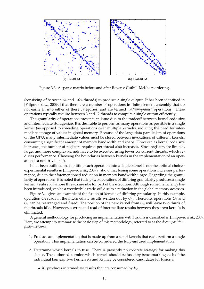
(a) Pre-RCM (b) Post-RCM

Figure 3.3: A sparse matrix before and after Reverse Cuthill-McKee reordering.

(consisting of between 64 and 1024 threads) to produce a single output. It has been identified in[Filipovic et al., 2009a] that there are a number of operations in finite element assembly that donot easily fit into either of these categories, and are termed medium-grained operations. Theseoperations typically require between 3 and 12 threads to compute a single output efficiently.

The granularity of operations presents an issue due to the tradeoff between kernel code sizeand intermediate storage size. It is desirable to perform as many operations as possible in a singlekernel (as opposed to spreading operations over multiple kernels), reducing the need for inter-mediate storage of values in global memory. Because of the large data-parallelism of operationson the GPU, many intermediate values must be stored between invocations of different kernels,consuming a significant amount of memory bandwidth and space. However, as kernel code sizeincreases, the number of registers required per thread also increases. Since registers are limited,larger and more complex kernels have to be executed using fewer concurrent threads, which re-duces performance. Choosing the boundaries between kernels in the implementation of an oper-ation is a non-trivial task.

It has been outlined that splitting each operation into a single kernel is not the optimal choice -experimental results in [Filipovic et al., 2009a] show that fusing some operations increases perfor-mance, due to the aforementioned reduction in memory bandwidth usage. Regarding the granu-larity of operations, it is noted that fusing two operations of differing granularity produces a singlekernel, a subset of whose threads are idle for part of the execution. Although some inefficiency hasbeen introduced, can be a worthwhile trade-off, due to a reduction in the global memory accesses.

Figure 3.4 gives an example of the fusion of kernels of differing granularity. In this example,operation O3 reads in the intermediate results written out by O1. Therefore, operations O1 andO3 can be rearranged and fused. The portion of the new kernel from O3 will leave two thirds ofthe threads idle. However, a write and read of intermediate results between these two kernels iseliminated.

A general methodology for producing an implementation with fusions is described in [Filipovic et al., 2009a].Here, we attempt to summarise the basic step of this methodology, referred to as the decomposition-fusion scheme:

1. Produce an implementation that is made up from a set of kernels that each perform a singleoperation. This implementation can be considered the fully-unfused implementation.

2. Determine which kernels to fuse. There is presently no concrete strategy for making thischoice. The authors determine which kernels should be fused by benchmarking each of theindividual kernels. Two kernels K1 and K2 may be considered candidates for fusion if:

• K1 produces intermediate results that are consumed by K2.

15

Multiprocessor

MultiprocessorO1: 3 threadsper element

O2: 9 threads

per element

O3: 1 thread

per element

O1: 3 threads

per element

O2: 9 threadsper element

O3: 1 thread

per element

O4: 1 thread

per elementO4: 1 thread

per element

Figure 3.4: Fusing kernels of different granularities. Left: Unfused kernels store results in globalmemory. Right: One pair of kernels is fused. From [Filipovic et al., 2009b].

• At least one of the kernels has high bandwidth utilisation and low computational in-tensity (in terms of GFLOPS/sec).

3. Create a new implementation in which the fusion candidates are fused.

4. Steps 2 and 3 may be repeated, until there are no fusion candidates.

Although this scheme can be used to produce implementations with a reasonable choice of fu-sions, there are several problems. Producing hand-implementations of the unfused implementa-tion is quite tedious. The criteria for finding fusion candidates are not well-defined. Furthermore,producing the implementations of the fused kernels will be a tedious and error-prone manualprocess. It is concluded that although it is necessary to search for an optimal fusion combinationto obtain the highest performance on GPU architectures, it would be highly desirable to automatethis process. The decomposition-fusion scheme will be impossible to implement practically in ageneral-purpose compiler, as it will be too difficult to perform an analysis that provides enoughinformation to automate the fusion. However, a compiler for a domain-specific language can bemade to produce a variety of fused and unfused kernels. The choice of which kernels are theoptimal ones may be guided by the development of a performance model, or by a profile-guidedalgorithm.

3.4 Colouring and Partitioning

Due to the parallel operation of the GPU, it is inevitable that there will be some contention whenwriting data. For example, if two elements share a node, the threads performing computation foreach of these elements will both need to update the same location. In order to prevent data races,techniques that can be used include the use of atomic operations, or colouring schemes.

The CUDA and OpenCL programming models provide support for certain atomic operationsthat can be used to implement atomic arithmetic operations on floating point numbers. Althoughthese operations ensure consistency, they can have a large impact on performance.

Colouring schemes may be used to remove the need for atomic operations, by ensuring thatentities whose updates may be in conflict have different colours. The execution proceeds in paral-lel over each colour, but each colour is processed sequentially. This prevents any contention.

It usually sufficient to perform the colouring using the Welch-Powell algorithm [Lipschutz and Lipson, 1997],which is a simple greedy algorithm, and is detailed in Algorithm 3. This algorithm is often suffi-cient as it is guaranteed to colour a graph with chromatic number ∆ using ∆ + 1 colours.

16

Algorithm 3: The Welch-Powell algorithm for colouring a graph G. From[Lipschutz and Lipson, 1997].

Order the vertices of G according to decreasing degrees ;1

Assign the first colour C1 to the first vertex and then, in sequential order, assign C1 to each2

vertex which is not adjacent to a previous vertex which was assigned C1 ;Repeat Step 2 with a second colour, C2 and the subsequence of non-coloured vertices ;3

Repeat Step 3 with a third colour, C3, then a fourth colour, C4, and so on until all vertices are4

coloured.

The use of a colouring scheme for avoiding atomic operations has been successfully appliedin the development of a large-scale earthquake model written in CUDA [Komatitsch et al., 2009,Komatitsch et al., 2010].

3.4.1 Oplus2

OPlus2 [Giles, 2010] is a general framework for programming unstructured mesh applications onGPUs that is currently under development. We draw attention to the proposed colouring schemefor avoiding atomic operations, in which the colouring is performed at two levels:

• In the first level of colouring, a partitioning of the mesh into chunks that are small enoughto be loaded into shared memory is made. These partitions are coloured such that no twoadjacent partitions share a colour. This allows chunks of the mesh to be loaded into sharedmemory and computed over by concurrently operating threads, without the risk of con-tention. A separate kernel invocation is used for each different colour of partition.

• The edges within partitions are also coloured, since OPlus2 performs computations on anedge-by-edge basis, rather than a node-by-node basis. The colouring for each partition is in-dependent of the colourings in other partitions. This colouring is used within the executionof one thread block on the chunk in shared memory. Executing kernels loop over the colourswithin the partition, to ensure that there is no contention between threads within a block.

It is expected that a similar 2-level scheme may be applied on a node-by-node basis to a meshin order to perform computations on data in shared memory in a finite element method imple-mentation in CUDA. However, the colouring is not strictly necessary in combination with thepartitioning if the Local Matrix Approach to the Global Assembly phase is adopted (See Section3.5.1 below).

3.5 Algebraic Transformations

The finite element method can be thought of as the composition of various algebraic operationson tensors [Kay, 1988]. It is possible to make transformations using algebraic operations in orderto derive equivalent formulations of a method. These transformations can increase the efficiencyof the method, either by reducing the operation counts, or by generating algorithms that are moreamenable to the target hardware.

In this section, we examine two transformations that are discussed in the literature; it is hy-pothesised that these transformations are just two of a large number of possibilities that may begenerated, and that each of the possible implementations will have different performance charac-teristics on different architectures.

3.5.1 Transforming the Global Assembly Phase

It was highlighted in Section 2.4 that the Addto algorithm is unlikely to be efficient on the GPUdue to its indirect accesses of data structures. Here we describe how the formulation of Equation

17

2.8 (representing the Global Assembly phase) may be transformed to avoid the use of the Addtoalgorithm.

An alternative algorithm, referred to as the Local Matrix Approach (LMA), is derived by notingthat the only use of M is for computation of the product Mv in the solution phase. We omit theglobal assembly of M (Equation 2.8) altogether, and when computation of y = Mv is required, thefollowing computation is performed:

y =(AT (Me (Av))

)(3.3)

This transformation involves making use of the associativity of matrix-matrix multiplication totransform the chain matrix multiplication of Equation 2.8 and the Matrix-vector product Mv intothe three matrix-vector products of 3.3. It is not possible to avoid the assembly of b, as it isexplicitly required by the solver. However, we can eliminate the use of the Addto algorithm bycomputing the matrix-vector product b = ATbe using an SpMV kernel.

We note that that the Local Matrix Approach uses more memory bandwidth and computationsthan the Addto algorithm. However, this increase in operations may be amortised by the reduc-tion in the use of inefficient memory accesses required by the Addto Algorithm. It has been shownin [Vos et al., 2009] and [Cantwell et al., 2010] that the Local Matrix Approach is more efficient thanthe Addto algorithm for certain polynomial bases when solving two- and three-dimensional prob-lems in CPU implementations.

3.5.2 Evaluation of Integral Forms by Tensor Representation

The FEniCS Form Compiler [Kirby and Logg, 2006] makes use of algebraic rearrangements to op-timise computations in the finite element method. Some of these optimisations are describedin [Logg, 2007]. In this subsection we reproduce the workings of one of the simpler optimisa-tions based on an algebraic transformation. This optimisation reduces the number of operationsrequired when evaluating integrals using Gaussian quadrature. This is achieved by making achange that allows more of the computational work to be performed on the reference element.This reduces the work needed to transform the solution from the reference element to the phys-ical element. Since the evaluation over the reference element is only performed once, whereasthe transformation is performed for every element, this optimisation greatly reduces the compu-tational cost of the overall computation.

We consider a transformation that may be applied when the mapping from the reference ele-ment to the physical element is affine. We consider a Laplacian form that may be evaluated usingGaussian quadrature as follows:

MeK[i, j] =

∫ΩK∇v · ∇u dX =

Nq

∑q=1

Ndim

∑α=1

wq∂φi

∂Xα(ξq)

∂φj

∂Xα(ξq)|JK| (3.4)

where wq is a quadrature weight, JK is the Jacobian of the transformation from reference spaceto physical space, and φ is a basis function in physical space. In order to derive the form thatperforms the transformation by a tensor contraction, we first write the dot product in the integralin terms of its components:

MeK[i, j] =

∫ΩK∇v · ∇u dX =

∫ΩK

Ndim

∑α=1

∂φi

∂Xα

∂φj

∂XαdX (3.5)

Next, we can make a change of variables from the physical coordinates to the coordinates on thereference cell, giving:

MeK[i, j] =

∫ΩK

Ndim

∑α=1

Ndim

∑β1=1

∂ξβ1

∂Xα

∂Φi

∂ξβ1

Ndim

∑β2=1

∂ξβ2

∂Xα

∂Φj

∂ξβ2

|JK| dX (3.6)

18

where ξ is a coordinate on the reference cell, and Φ is a basis function on the reference cell. Sincethe mapping from the reference element to the physical element is affine, the sums ∑Ndim

β∂ξ∂X and

the determinant |JK| are constant throughout the element, and can be moved outside the integral:

MeK[i, j] = |JK|

Ndim

∑α=1

Ndim

∑β1=1

∂ξβ1

∂Xα

Ndim

∑β2=1

∂ξβ2

∂Xα

∫ΩK

∂Φi

∂ξβ1

∂Φj

∂ξβ2

dX (3.7)

This can be written as a tensor contraction:

MeL[i, j] =

Ndim

∑β1=1

Ndim

∑β2=1

AijβGβK ⇒ Me = A : GK (3.8)

where

Aijβ =∫

ΩK

∂Φi

∂ξβ1

∂Φj

∂ξβ2

dX, GαK = |JK|

Ndim

∑α=1

∂ξβ1

∂Xα

∂ξβ2

∂Xα(3.9)

This optimisation reduces the number of arithmetic operations required from Nqn20d to d3 +

N20 d2 ∼ n2

0d2 where Nq is the number of quadrature points, n0 is the polynomial order of the basis,and d is the number of dimensions. Since the number of dimensions is almost always 2 or 3, thereduction in operations is roughly a factor of Nq, which can be a significant reduction for highorder basis functions.

We remark that although this particular example is specific to the Laplacian form, the key partof this optimisation is the change of variables, which may be applied to any integral form. Thereare other examples of similar optimisations that may be used in cases when the transform fromthe reference element to the physical element is not affine, discussed in [Kirby and Logg, 2006]and [Logg, 2007].

It is thought that this transformation is part of a more general class of transformations thatreduces the operation count of constructing the global matrix and global vector. These operationsare based around rewriting terms under an integral, in order that part of the rewritten term be-comes constant over an element. These newly-created constant terms can be moved outside theintegral in order to reduce the complexity of the computations that need to be performed for everyelement.

3.6 Related Areas

In this section we examine literature that is not directly related to the finite element method, butfrom which we can draw ideas that may integrate well with the proposed research. We suggesthow these ideas may be relevant to the development of our project.

3.6.1 Library Generators

A number of tools for generating optimised libraries for specific domains exist, including Built ToOrder BLAS [Belter et al., 2009, Jessup et al., 2010] for linear algebra, SPIRAL [Puschel et al., 2005]for DSP transforms, and the Tensor Contraction Engine [Auer et al., 2006]. We discuss SPIRAL andthe Tensor Contraction Engine in more detail below in order to discuss concepts that could alsobe applied to the generation of finite element solvers.

SPIRAL

SPIRAL [Puschel et al., 2005] is a platform for generating highly efficient code for DSP transforms.The motivation for its development is the observation that traditional compilers do a poor jobof optimising C code for DSP transforms. This is because the C code contains no semantic in-formation regarding the choice of algorithm, so the compiler is forced to make the most generalassumptions about the code, inhibiting optimisation.

19

DSP transforms are defined using the Signal Processing Language (SPL), which uses a matrixalgebra representation. SPL constructs are manipulated according to a set of rules that allow acomplex transform to be rewritten in terms of simpler ones (e.g. the Cooley-Tukey rule), or thatperform algebraic rewrites by using matrix identities. These rules may be repeatedly applied togenerate a broad class of algorithms that perform the same computation.

The various implementations are converted into an SSA-form [Aho et al., 2006] intermediaterepresentation (Σ-SPL). Standard optimisations including loop unrolling, intrinsic precomputa-tion, common subexpression elimination etc. are applied to this representation. These optimisedrepresentations are converted to scalar C code or vector code using intrinsics for the target plat-form. The choice of vector intrinsics is influenced by a description of the available operations onthe target hardware. A similar process is used to generate code for multiprocessor systems andGPUs, although this work is still under development [SPIRAL Project, 2010].

There is a large variation in the performance of the generated implementations of transforms.In order to select the best implementations, learning and search techniques are used. The learningframework is used to prune the search space by removing candidate implementations that areexpected to perform poorly, based on automatically built performance models of the operationsthat constitute each implementation. Dynamic programming [Bellman, 2003] and evolutionarysearch [Goldberg, 1989] are used to find the best candidates in the remaining space of possibleimplementations.

We remark that there is almost a direct analogy between SPIRAL and the FEniCS tools. Inboth projects, high-level domain-specific languages are used as a source from which to generateoptimised code. It is conjectured that the techniques used in SPIRAL to generate efficient DSPtransforms may be translated to generate efficient implementations of finite element codes onGPUs. In particular, the idea of using a rulebase to guide transformations of an algorithm isapplicable to the finite element method, as demonstrated in Section 3.5. The generation of a spaceof possible implementations of finite element algorithms may also necessitate mechanisms forpruning the search space.

We also note that techniques for searching for the optimal implementation may also be appliedat a lower level: there is a space of possible kernel fusions that may be made, and some mechanismfor searching this space will be required. Additionally, characteristics of the target hardware suchas the L1 cache size, the number of SMs on the device, and the number of registers etc. may formpart of a performance model that is used to guide this search.

The Tensor Contraction Engine

The Tensor Contraction Engine [Auer et al., 2006, Baumgartner et al., 2002] is used for searchingfor the best implementation of tensor contractions, given restrictions on storage space at variousmemory hierarchy levels. We consider an example given in [Baumgartner et al., 2002]:

Sabij = ∑cde f kl

Aacik × Bbe f l × Cd f jk × Dcdel (3.10)

This expression may be evaluated using ten nested loops in 4× N10 operations, where the rangeof each index is N. The same result can be computed in 6× N6 operations by rearranging theexpression:

Sabij = ∑ck

(∑d f

(∑e f

Bbe f l × Dcdel

)× Dd f jk

)× Aacik (3.11)

However, this new expression requires a large amount of temporary storage, which may exceedthe memory capacity of the target machine. There are a large set of expressions that perform anequivalent computation to Equations 3.10 and 3.11, requiring various amounts of computationand storage. Manipulation of the tensor expression to produce various different versions is rela-tively straightforward, especially using a package such as Matlab [MathWorks, 2009]. However,

20

continuous (* Pendulum physics *)

m = 5.0; g = 9.81; l = 3;

I = m * l^2;

F*l*cos(theta) - m*g*l*sin(theta) = I*theta’’;

boundary conditions

theta with theta(0) = 0.1, theta’(0) = 0;

Figure 3.5: An Acumen description of the physics of a pendulum. Note that theta is an indepen-dent variable that changes over time. From [Zhu et al., 2010].

producing an implementation of the computation and benchmarking it requires a relatively largeeffort to implement the trivial code needed to implement each expression.

In order to overcome this problem, the TCE provides a domain-specific language for writingdown a tensor expression. An optimal implementation of the expression that requires a minimalamount of computation given memory and disk space limits is searched for, and an implemen-tation is automatically generated. This greatly reduces the burden on the programmer in imple-menting tensor contraction operations.

A similar situation arises in the implementation of finite element methods on GPUs. Using agreater number of smaller kernels increases the total number of threads that can run concurrentlyand increases performance. However, using more kernels requires more intermediate storagearrays. In this case, the use of memory bandwidth rather than memory space becomes an issue, asthe performance of the kernels becomes limited by their ability to transfer data to and from globalmemory. Out of these possible implementations, a search is required to find the optimum kernelgranularity subject to the constraints on the occupancy of individual kernels.

3.6.2 Acumen

The Acumen system [Zhu et al., 2010] provides the user with a domain-specific language for spec-ifying the ordinary differential equations governing a mechanical system. Figure 3.5 gives a shortexample of the Acumen source describing a pendulum. The Acumen compiler performs someanalysis and transformation on the equations in the source file, in order to transform them into asystem that can be stepped forward in time using a Runge-Kutta method.

The system of equations go through several phases of analysis and transformation in order toreach their final form, including a defined variable analysis, binding time analysis, and symbolicdifferentiation. A key contribution of the Acumen system is the binding time analysis, that isused to provide information to the symbolic differentiation phase that allows it to reduce thecomplexity of the generated expression. In contrast, tools such as Matlab must make more generalassumptions about equations they are differentiating symbolically, leading to the generation ofmuch larger expressions than are required.

Although we do not cover this defined variable analysis in detail, we note that at the heart ofthis transformation is the concept of using domain-specific knowledge to reduce the complexityof the generated code. The use of similar analyses in the finite element context might be used toreduce the complexity of the code for evaluating multilinear forms, perhaps as part of a systemthat performs algebraic transformations of the forms.

3.6.3 Autotuning Libraries

Self-tuning libraries for particular domains maximise performance on a particular target by per-forming extensive benchmarking and tuning at installation time. There are examples of these li-braries for a number of different domains, including ATLAS [Whaley and Dongarra, 1998, Whalley, 2005]for linear algebra, OSKI [Vuduc et al., 2005, Vuduc, 2003] for sparse matrix operations, and FFTW

21

[Frigo and Johnson, 2005] for Fourier transforms. The search performed at installation time canbe very time-consuming, but only needs to be performed once.

Since the performance characteristics can vary from machine to machine depending on factorssuch as the number of cores, number of processors, size and latency of each level in the memoryhierarchy etc., the use of automatic tuning ensures that the best possible implementation is usedon each machine. In relation to implementations of the finite element method, we note that thesearch space of implementations when considering various algebraic rewrites as well as kernelfusions and other optimisations may become large. In the absence of more sophisticated searchtechniques, performing brute-force autotuning to generate the best implementation of a solver fora particular UFL source may be an option.

3.6.4 Active Libraries

Active Libraries [Czarnecki et al., 2000] perform optimisation of computations by generating spe-cialised implementations, at runtime or at compile time using expression templates. Active li-braries include DESOLA for linear algebra [Russell et al., 2008], Blitz++ [Veldhuizen, 1998] andthe Matrix Template Library [Siek, 1999] for matrix operations, and Bernoulli for sparse matrixoperations [Ahmed et al., 2000].

A feature that these libraries have common is that they are all designed to be used from inside alow-level language, such as C++, rather than as part of a domain-specific language. Since the UFLrepresentation is high-level and retains necessary semantic information about the computations,it is difficult to map the techniques used by active libraries onto code generation of finite elementmethods using UFL.

3.6.5 Formal Linear Algebra Methods Environment

The Formal Linear Algebra Methods Environment (FLAME) [Gunnels et al., 2001, Bientinesi et al., 2005]systematises the development of linear algebra algorithms and their translation into code. In orderto derive an algorithm, a worksheet is filled in according to conditions on the input and expectedoutput of the algorithm, and also conditions that are required to hold throughout the execution ofthe algorithm. The completed worksheet specifies the resulting algorithm in an inductive fashion.Although the worksheet must be filled in by hand, there have been some efforts directed towardsautomatically deriving the filled-in worksheet [Bientinesi, 2006]. The methodology has recentlybeen extended to the derivation of Krylov-subspace solvers [Eijkhout et al., 2010] (examples ofKrylov-subspace solvers include the conjugate gradient and GMRES methods).

It is remarked that there is a similarity between the work in [Bientinesi, 2006] on automaticallyderiving new algorithms, and the techniques used to derive new implementations by makingalgebraic transformations in SPIRAL, and those described in Section 3.5. The inductive nature ofthe algorithms produced by worksheet fill-in are substantially different from any of the knownalgebraic transformations of finite element operations. However, it is possible that formulationsof the finite element method in terms of tensor contractions can be treated in this fashion. Thiscould be investigated if it is difficult to find transformation rules of finite element operations interms of algebraic operations.

3.7 Conclusions

We have examined the Unified Form Language from the FEniCS project, which provides a meansfor declaratively specifying a finite element method. Since the UFL representation is completelyindependent of the underlying implementation, all of the optimisation techniques that have beenexamined throughout this chapter may be implemented in a UFL compiler without exposing themto the user. The compilation and optimisation techniques that can be pursued as part of furtherinvestigations can be summarised as follows:

22

Data layout transformations. Partitioning and padding techniques that allow more effective useof the memory hierarchy have been described in Sections 3.4 and 3.3.1 respectively.

Colouring. Using colouring schemes avoids the need for atomic operations on GPUs, increasingefficiency. The OPlus2 two-level scheme works in conjunction with partitioning, and imple-mentation of this scheme should be investigated.

Kernel Granularity. Section 3.3.3 outlined the necessity for choosing the appropriate level ofgranularity of kernels, and described a scheme for finding an efficient choice of kernel fu-sions.

Algebraic Transformations. In Section 3.5, two examples of algebraic transforms are outlined. Itis hypothesised that many algebraic transforms are possible, and that these possible trans-forms may be enumerated as a set of transformation rules. The implementation space gener-ated by these transformations may be explored using techniques similar to those in SPIRALand the Tensor Contraction Engine, described in Section 3.6.1.

Automatic Tuning. Automated search and tuning techniques (Section 3.6.3) can be used in con-junction with techniques that generate a space of possible implementations, including analgebraic transformation system and a lower level system for generating implementationsof different kernel granularities.

Manual investigations of these areas will be time-consuming. In order to reduce the time takento perform investigations, and to work towards the eventual goal of providing tools that automat-ically generate efficient GPU implementations of finite element solvers from high-level sources,it is pragmatic to begin by implementing a UFL compiler that generates GPU implementations.This can then be followed by the implementation of these transformations and optimisations inthe code generator. The following chapter describes preliminary investigations into some of theseareas that have already taken place. Chapter 5 goes on to describe a plan for carrying out thisresearch over the course of the PhD.

23

24

Chapter 4

Preliminary Investigations

4.1 Introduction

In this chapter we describe some experiments that investigate the performance of two algorithmsfor the global assembly phase on the GPU, and a prototype implementation of a UFL compiler.The content of this chapter has been published as part of [Markall et al., 2010c].

A complete implementation of a test problem has been developed that executes all computa-tions on the GPU, and this is used as the basis for our experiments. We also discuss a data layouttransformation that was necessary to obtain coalescing, and therefore make use of a substantialportion of the available memory bandwidth of the device. These experiments show that the opti-mal algorithm depends on the target hardware.

The implementation of the prototype UFL compiler that generates CUDA code is also de-scribed. The performance of the generated code is not investigated, but instead we use the ex-perience gained from this exercise to map out the future work that needs to be done in order toimplement a more complete compiler.

4.2 Data Format Considerations

In general, data structures must be carefully chosen to achieve optimal performance (e.g. forcache-optimality on a CPU), and the optimal choice of data structure depends on characteristicsof the target architecture. In order to examine the structures that can be used when implementingthe finite element method on CPUs and GPUs, we consider a three element domain (see Figure4.1).

In CPU implementations, nodal data is often stored on a per-node basis. When data for thenodes of a single element is needed, the mapping array (map) is used to indirectly access the nodaldata. Although this can lead to poor cache performance due to random access into the nodal datastructure, reordering optimisations can be used to minimise this overhead.

This data format is inefficient for GPU implementations, where coalesced accesses must beused to maximise memory performance. It is difficult to achieve coalesced access because the

AB

C1 2

5

3

4 12 1 5 23 2 4 34 4 2 55 A B C

Figure 4.1: Left: A 2D domain decomposed into three elements. Middle: Node data layout in CPUimplementation. Right: Node data layout in GPU implementation. Threads accessing data indifferent elements (arrowed) achieve coalescing.

25

nodal data structure is accessed in a somewhat random fashion. We propose that it can be moreefficient to store nodal data on a per-element basis in GPU implementations, interleaving the nodaldata for each node of each element. This leads to some redundancy in the storage of nodal data,again proportional to the average variance of nodes; however, it allows coalesced accesses whenthere is a one-to-one mapping between threads and elements.

4.3 Experiments

We evaluate the performance of the Addto algorithm and the Local Matrix Approach on GPUsusing an implementation of a test problem that solves the advection-diffusion equation:

∂T∂t

+ u∇T = ∇ · µ · ∇T

where T is the concentration of a tracer, t is time, u is velocity, and µ is a rank-2 tensor of diffusivity.This problem is chosen as it is both a sub-problem and simplified model of a full computationalfluid dynamics system. The system is discretised using order-1 basis functions. A split schemeis used, solving for advection first and then diffusion at each time step. The advection term istimestepped using a 4th-order Runge-Kutta scheme, and the diffusion term is timestepped us-ing an implicit theta scheme. The problem is solved over a square domain with suitable initialconditions. We compare with a CPU implementation to demonstrate that the optimal choice ofalgorithm depends on the target hardware.

4.3.1 CUDA and CPU Implementations and Experimental Setup

CUDA Implementations of the solver that implement both the Addto algorithm and the Local Ma-trix Approach have been produced. The Local Matrix Approach is implemented by consideringthe computation in Equation 3.3 in three stages:

t = Av︸ ︷︷ ︸Stage 1

, t′ = Met︸ ︷︷ ︸Stage 2

, y = ATt′︸ ︷︷ ︸Stage 3

.

Since A contains only one non-zero entry per row that is always 1, Stage 1 is implemented asa gather. This involves uncoalesced memory accesses but is more efficient than using an SpMVkernel. The implementation of Stage 2 exploits the block-diagonal structure of Me to achievecoalesced accesses and maximal reuse of matrix values. Stages 1 and 2 are implemented in a singlekernel. Stage 3 is implemented as an SpMV kernel that is optimised for all the non-zero valuesequalling 1. Because a global barrier is required between Stages 2 and 3, Stage 3 is implementedin a separate kernel.

The baseline version is implemented within Fluidity because it is a mature and optimised CPUimplementation. The Local Matrix Approach is not implemented in this version, as it is known tobe less efficient than the Addto algorithm on CPUs for low-order basis functions [Vos et al., 2009].Node data structures are implemented using the element-wise storage layout in the CUDA imple-mentation, and the node-wise layout is used in the CPU implementation.

The test hardware consists of an Intel Core 2 Duo E8400, 2GiB RAM, and an NVidia 280GTXGPU. The Intel v10.1 compilers with the -O3 flag were used for the CPU code (v11.0 onwards can-not compile Fluidity due to compiler bugs), and the CUDA SDK 2.2 is used for CUDA code. TheCUDA implementation uses a Conjugate Gradient (CG) solver described in [Markall and Kelly, 2009];the baseline version make use of the PETSc [Balay et al., 2009] CG solver. The simulation is run for200 timesteps, with all computations using double precision arithmetic. Gmsh [Geuzaine and Remacle, 2009]was used to generate meshes varying in size between 28710 and 331714 elements. Each simulationwas run five times, and averages are reported.

26

4.3.2 Results

Figure 4.2 shows the total time taken by each CUDA implementation to run the entire simulation.Figure 4.3 shows their speedup relative to the baseline version running on 2 cores. We see that theLMA implementation is up to 2.2 times faster than the Addto implementation on the GPU, and isover an order of magnitude faster than the baseline implementation.

0

20

40

60

80

100

50000

100000

150000

200000

250000

300000

Tim

e(s

)

Number of Elements

LMA, SpMV for RHSAddto for Matrix and RHS

Figure 4.2: Total execution time of GPU implementations.

Figure 4.4 shows the total time taken for the local and global assembly phases in the CUDAimplementations. We observe that the Local Matrix Approach is faster than the Matrix Addto al-gorithm, and that it is faster to assemble the global vector by computing the productATbe. Figure4.1 shows the total time spent inside the SpMV kernels for each implementation for the largest andsmallest mesh sizes. The cost of computing

(AT (Me (Av))

)(in the LMA implementation) is up to

2.5 times that of computing Mv (in the Addto implementation). The performance increase of theLMA implementation is a tradeoff between the decrease in the assembly time, and the increase inthe SpMV computation time.

Elements(AT (Me (Av))

)Mv

28710 1.91× 106 8.48× 105

331714 2.45× 107 9.85× 106

Table 4.1: Total time spent computing each product on the largest and smallest meshes (in µsec),recorded using the CUDA Profiler.

We also investigated using graph colouring to eliminate atomic operations in the Addto im-plementation (as used in [Komatitsch et al., 2009]). We replaced atomic operations with equiva-lent non-atomic operations. The resulting implementation produced incorrect results, but gave anupper bound on the performance increase facilitated by colouring. The assembly phase ran 25%faster with non-atomic operations, corresponding to a 10% speedup in the entire simulation. Sincethe performance of the LMA implementation is far greater than this, it is unnecessary to producean implementation that uses colouring.

27

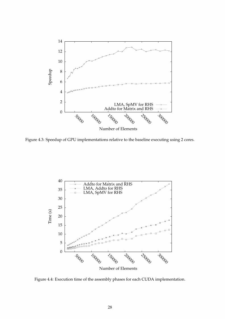
0

2

4

6

8

10

12

14

50000

100000

150000

200000

250000

300000

Spee

dup

Number of Elements

LMA, SpMV for RHSAddto for Matrix and RHS

Figure 4.3: Speedup of GPU implementations relative to the baseline executing using 2 cores.

0

5

10

15

20

25

30

35

40

50000

100000

150000

200000

250000

300000

Tim

e(s

)

Number of Elements

LMA, SpMV for RHSLMA, Addto for RHSAddto for Matrix and RHS

Figure 4.4: Execution time of the assembly phases for each CUDA implementation.

28

4.4 Further Investigations

Our results show that the optimal algorithm depends on the target architecture. We speculate thatit is also problem-dependent. In a 2D domain the average variance of nodes is approximately6. In a 3D domain, the variance is around 24, and the overheads of storage and computation forthe local matrix approach are four times greater than in 2D. This extra overhead may decreaseperformance to the point where it is more efficient to use the Addto algorithm. Our further workinvolves investigating the performance in this case.

4.5 A Prototype Compiler

A first step in experimenting with generating CUDA code from UFL involved the implementationof a compiler that performs a syntax-directed translation of the UFL code to CUDA code. The gen-erated code uses a library of kernels that perform common operations in finite element assembly.A subset of the kernels in this library are shown in Table 4.2. These kernels perform quadrature-based assembly, rather than the tensor-based method that is used in the FEniCS project.

The compiler inputs UFL using the FEniCS UFL distribution [Alnæs and Logg, 2009] to pro-duce Directed Acyclic Graphs (DAGs) of the operations specified in a UFL source. Each DAGnode is converted to a call to a kernel implementing the required operation. This DAG of kernelcalls is passed to a code generator that is implemented using the ROSE Compiler Infrastructure[Quinlan et al., 2009]. Examples of the DAGs for the left-hand side of Equation 3.2 are shown inFigure 4.5.

v u

∇v ∇u

∇v · ∇u

A

(a) Expression DAG.

tform shape(v) tform shape(u)

tform dshape(v) tform dshape(u)

dshape dot dshape

mat addto

(b) Kernel DAG.

Figure 4.5: DAGs for the form∫

Ω∇v · ∇u dX.

Kernel Operationtform shape Transform basis functions from reference space to physical space.tform dshape Transform derivatives of basis functions to physical space.

dshape dot dshape Computes∫

Ω∇v · ∇u dX.shape shape Computes

∫Ω vu dX.

mat addto Adds local matrices into a global matrix using the Addto algorithm.

Table 4.2: A subset of kernels in the CUDA kernel library.

The CUDA code generated by this compiler for the Poisson problem produces identical resultsto a handwritten CUDA implementation, as well as a CPU implementation of the same problem.Although the generated code executes faster than the CPU implementation for large meshes, wedo not investigate its performance as there is only a limited speed improvement that can be gainedfor steady-state problems.

4.5.1 Further UFL Compiler Development

Although the prototype compiler demonstrates the feasibility of generating CUDA code fromUFL sources, the requirement for a library of handwritten CUDA kernels limits its output to a

29

pre-defined set of forms optimised by hand. Here we describe an intermediate phase that low-ers the UFL representation to one amenable to optimisation with established techniques beforebeing used to generate CUDA kernels. Consider one term from the weak form of the Helmholtzequation [Karniadakis and Sherwin, 1999]:∫

Ω∇v · ∇u + λvu dX (4.1)

There are several combinations of kernels that implement the local assembly phase of thisterm that can be implemented. We can enumerate these possibilities by building an IntermediateRepresentation (IR) that provides a high-level semantic representation of each term. Sub-terms ofthe intermediate representation are determined by working bottom-up from leaf nodes to identifythe smallest set of nodes that describes the assembly of a local matrix. Higher sub-terms areidentified as the addition or scalar multiplication of lower-sub terms.

The IR for Equation 4.1 is shown in Figure 4.6. As there are four sub-terms, up to four sepa-rate kernels may perform local assembly for this term. Using more kernels increases the memorybandwidth requirements; however, larger kernels require more resources, decreasing the totalparallelism [Filipovic et al., 2009a]. Instead of building a performance model to evaluate each can-didate implementation, a pragmatic approach is to lower this representation to one that can beoptimised using existing techniques.

Each of the nodes at the root of the sub-terms may be lowered to a loop over a certain index.For example, the sum node corresponds to a loop over the elements that sums the local matri-ces produced by the lower sub-terms. The generated loop nest can be optimised using standardtechniques, for example in the polyhedral model [Pouchet et al., 2007] or the Æcute framework[Howes et al., 2009].

dX

sum

dot scalarproduct

grad grad λ outerproduct

v u v u

Figure 4.6: Intermediate Representation of the term∫

Ω∇v ·∇u+λvu dX. Sub-terms are indicatedby dotted outlines.

4.6 Conclusions

The experimental results that have been presented have shown that the Local Matrix Approachgives superior performance compared to the Addto algorithm when implementing the finite el-ement method on a GPU in 2D using order-1 basis functions. We have also seen that changes inthe data format and the structure of the assembly loop are necessary. All of these changes arerepresented by the same UFL source code, and a compiler is free to make choices about each ofthese aspects.

We have also discussed the implementation of a prototype UFL compiler that generates codereliant on a library of hand-written local matrix assembly kernels. Since we have found that thisis not an efficient approach, current work is based upon reimplementing this compiler so thatit generates kernels based on specific forms that are in the UFL source. A suitable intermediaterepresentation has been outlined. It is expected that this representation will allow the generation

30

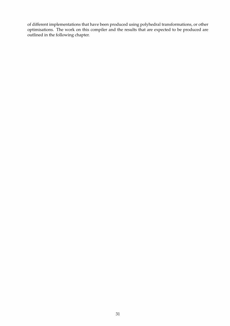
of different implementations that have been produced using polyhedral transformations, or otheroptimisations. The work on this compiler and the results that are expected to be produced areoutlined in the following chapter.

31

32

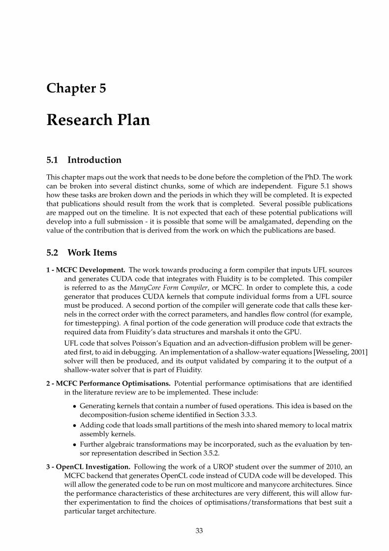
Chapter 5

Research Plan

5.1 Introduction

This chapter maps out the work that needs to be done before the completion of the PhD. The workcan be broken into several distinct chunks, some of which are independent. Figure 5.1 showshow these tasks are broken down and the periods in which they will be completed. It is expectedthat publications should result from the work that is completed. Several possible publicationsare mapped out on the timeline. It is not expected that each of these potential publications willdevelop into a full submission - it is possible that some will be amalgamated, depending on thevalue of the contribution that is derived from the work on which the publications are based.

5.2 Work Items

1 - MCFC Development. The work towards producing a form compiler that inputs UFL sourcesand generates CUDA code that integrates with Fluidity is to be completed. This compileris referred to as the ManyCore Form Compiler, or MCFC. In order to complete this, a codegenerator that produces CUDA kernels that compute individual forms from a UFL sourcemust be produced. A second portion of the compiler will generate code that calls these ker-nels in the correct order with the correct parameters, and handles flow control (for example,for timestepping). A final portion of the code generation will produce code that extracts therequired data from Fluidity’s data structures and marshals it onto the GPU.

UFL code that solves Poisson’s Equation and an advection-diffusion problem will be gener-ated first, to aid in debugging. An implementation of a shallow-water equations [Wesseling, 2001]solver will then be produced, and its output validated by comparing it to the output of ashallow-water solver that is part of Fluidity.

2 - MCFC Performance Optimisations. Potential performance optimisations that are identifiedin the literature review are to be implemented. These include:

• Generating kernels that contain a number of fused operations. This idea is based on thedecomposition-fusion scheme identified in Section 3.3.3.• Adding code that loads small partitions of the mesh into shared memory to local matrix

assembly kernels.• Further algebraic transformations may be incorporated, such as the evaluation by ten-

sor representation described in Section 3.5.2.

3 - OpenCL Investigation. Following the work of a UROP student over the summer of 2010, anMCFC backend that generates OpenCL code instead of CUDA code will be developed. Thiswill allow the generated code to be run on most multicore and manycore architectures. Sincethe performance characteristics of these architectures are very different, this will allow fur-ther experimentation to find the choices of optimisations/transformations that best suit aparticular target architecture.

33

Jul

Aug

Sep

Oct

Nov

Dec

Jan

Feb

Mar

Apr

May

Jun

Jul

Aug

Sep

Oct

Nov

Dec

Jan

Feb

Mar

Apr

May

Jun

Jul

Aug

Sep

2010:

2011:

2012:

1. Work on development of MCFC. Use to generate:test_laplaciantest_advection_diffusionshallow_water_solver

2. Implement performance optimising transformationsin MCFC. These include: - Manually-implemented algebraic transformations - Kernel fusions - Data layout and memory hierarchy optimisations

4. Develop a framework foralgebraic transformations ofthe Finite Element Method.

3. Investigate OpenCLcode generation and execution on otherGPU architecturesand CPUs.

5. Prototype integration of generatedcode into Fluidity. Developmentof schemes to improve data marshalling. Testing the codefor discretisations of various PDEs.

7. Writing-up period. Includesperforming extra experimentsneeded to complete the thesisand reviewing recent literature.

8. Production-level integration ofgenerated code into Fluidity.Work with users to correct bugsand implement portions of anocean model in UFL.

Potential Paper 1

Potential Paper 2

Potential Paper 3

Potential Paper 4

Potential Paper 5

6. Work towards making generation of a fullNavier-Stokes solver possible.This requires support for: - Picard iteration - Pressure projection

Figure 5.1: Timeline showing tasks until the completion of the PhD.

34

4 - Algebraic Transformations. Similarly to the SPIRAL project, it is expected that the Finite Ele-ment Method may be represented as a set of algebraic operations that may be transformedby a set of rules, to generate a whole space of possible implementations. It is expected thatthe optimal choice of transformations is different for each architecture, and it is hoped that itis possible to develop methods to guide the transformations with a knowledge of the targetarchitecture.

5 - Fluidity Integration. Since one of the main goals of this project is to provide tools for automat-ically generating code to the users/developers of Fluidity, it is necessary to consider how thegenerated code integrates into Fluidity on a large scale. This work unit will involve experi-menting with integrating generated code into the main Fluidity codebase. Due to the size ofFluidity and the various non-finite element operations that it performs (such as mesh adap-tivity). It is expected that issues will arise in managing data placement and ensuring thatdata freshness is maintained across different architectures. Accordingly, a large proportionof time has been set aside to overcome these issues whilst still maintaining performance.

6 - Navier Stokes. Since the motion of fluids is generally described by the Navier-Stokes equa-tions [Wesseling, 2001], and form a large part of the numerical computations in Fluidity, it isimportant to work towards the generation of a solver for these equations from UFL sources.In order to achieve this, MCFC must be extended to generate code for Picard iteration, inorder to compute the nonlinear term.

7 - Writing Up. The thesis will be finalised at this stage. Further experiments that are required tocomplete the research may also be run at this stage.

8 - Fluidity Deployment. The tools for generating code will be passed on to the developers ofFluidity, and used to integrate generated code that assembles a large portion of the systemsthat are solved in Fluidity. This will include the implementation of terms such as gravity,buoyancy, surface tension, viscous, coriolis geostrophic pressure etc. It is hoped that therewill be two-way communication with developers, leading to improvements in MCFC as wellas bugfixes and usability improvements. The experiences from this work item will also beintegrated into the thesis in Work Item 7.

5.3 Potential Publications

1. This publication is based upon the work completed in Work Item 1. The expected contri-bution includes a description of the implementation of MCFC. This is novel since there arecurrently no compilers for UFL that generate CUDA code, and because the issues arisingfrom the implementation are non-trivial. It is expected that some code-generation choiceswill be embedded into MCFC, including the choice of either the Local Matrix Approach orthe Addto algorithm. Performance results for each of the implementations may be comparedin the publication.

2. This publication is based upon the work in Work Items 2 and 4, and possibly 3. The contribu-tion will be the presentation of the algorithms for performing algebraic transformations onfinite element implementations, and a discussion of the rules contained within the rulebase.Performance results for various architectures that demonstrate how the choice of transfor-mations affects the performance will be presented.

3. This publication is based upon the Work Item 5. The contribution will be based around thework needed to integrate generated code into Fluidity, in particular the techniques requiredto maintain consistency of data across different nodes and architectures, whilst maintainingperformance by transferring data efficiently.

4. This publication is based on Work Item 6, and will discuss the implementation and perfor-mance of the Navier-Stokes solver on CPU and GPU architectures. It is expected that part

35

of the contribution will describe the efficient implementation of boundary conditions onmanycore architectures.

5. This publication is based on all the Work Items, and is expected to be an article summaris-ing the state of the research, and in particular drawing attention to the large-scale modelsthat are able to be simulated with generated code, as well as the improvement in softwaredevelopment that is brought about by the use of a high-level language for development.

6. Another publication that can be developed relatively independently of the other work in thetimeline involves determining the grammar for UFL, and assigning a semantics and typesystem to the constructs generated by this grammar. This will provide a contribution to thecommunity, since there is presently no formal definition of UFL.

5.4 Conclusions

The research that has been completed so far has laid the foundations for the development of toolsfor generating high-performance finite elements solvers on manycore architectures. The eventualgoal of this research is to provide these tools to users that will benefit from them, both in terms ofease of development and the performance of the resulting code.

The long-term goal (beyond the scope of this PhD) is to rewrite a large portion of Fluidityusing UFL. The result of this work will be a portable and maintainable high-performance codethat allows aggressive exploitation of future architectures.

36

Bibliography

[Ahmed et al., 2000] Nawaaz Ahmed, Nikolay Mateev, and Keshav Pingali. A framework forsparse matrix code synthesis from high-level specifications. In Supercomputing ’00: Proceed-ings of the 2000 ACM/IEEE conference on Supercomputing (CDROM), page 58, Washington, DC,USA, 2000. IEEE Computer Society.

[Aho et al., 2006] Alfred V. Aho, Monica S. Lam, Ravi Sethi, and Jeffrey D. Ullman. Compilers:Principles, Techniques, and Tools (2nd Edition). Addison Wesley, August 2006.

[Alnæs and Logg, 2009] Martin Alnæs and Anders Logg. UFL Specification and User Manual 0.1.URL: http://www.fenics.org/pub/documents/ufl/ufl-user-manual/ufl-user-manual.

pdf, April 2009.

[AMD, 2010] AMD. AMD: Unleashing the power of parallel compute. http://sa09.idav.

ucdavis.edu/docs/SA09_AMD_IHV.pdf, retrieved 10 June 2010, 2010.

[Auer et al., 2006] A.A. Auer, G. Baumgartner, D.E. Bernholdt, A. Bibireata, V. Choppella, D. Co-ciorva, X. Gao, R. Harrison, S. Krishnamoorthy, S. Krishnan, et al. Automatic code generationfor many-body electronic structure methods: the tensor contraction engine. Molecular Physics,104(2):211–228, 2006.

[Bagheri and Scott, 2004] Babak Bagheri and L. Ridgway Scott. About Analysa. Technical ReportTR-2004-09, University of Chicago, 2004.

[Balay et al., 2009] Satish Balay, Kris Buschelman, William D. Gropp, Dinesh Kaushik, Matthew G.Knepley, Lois Curfman McInnes, Barry F. Smith, and Hong Zhang. PETSc Web page, 2009.http://www.mcs.anl.gov/petsc.

[Bangerth et al., 2007] W. Bangerth, R. Hartmann, and G. Kanschat. deal. IIA general-purpose object-oriented finite element library. ACM New York, NY, USA, 2007.

[Baumgartner et al., 2002] G. Baumgartner, D.E. Bernholdt, D. Cociorva, R. Harrison, S. Hirata,C.C. Lam, M. Nooijen, R. Pitzer, J. Ramanujam, and P. Sadayappan. A high-level approachto synthesis of high-performance codes for quantum chemistry. In Proceedings of the 2002ACM/IEEE conference on Supercomputing, pages 1–10. IEEE Computer Society Press Los Alami-tos, CA, USA, 2002.

[Bellman, 2003] Richard Bellman. Dynamic Programming. Dover Publishing, 2003.

[Belter et al., 2009] Geoffrey Belter, E. R. Jessup, Ian Karlin, and Jeremy G. Siek. Automating thegeneration of composed linear algebra kernels. In SC ’09: Proceedings of the Conference on HighPerformance Computing Networking, Storage and Analysis, pages 1–12, New York, NY, USA, 2009.ACM.

[Bientinesi et al., 2005] Paolo Bientinesi, John A. Gunnels, Margaret E. Myers, Enrique S.Quintana-Ortı, and Robert A. van de Geijn. The science of deriving dense linear algebra al-gorithms. ACM Transactions on Mathematical Software, 31(1):1–26, March 2005.

37

[Bientinesi, 2006] Paolo Bientinesi. Mechanical Derivation and Systematic Analysis of Correct LinearAlgebra Algorithms. PhD thesis, The University of Texas at Austin, Department of ComputerSciences, August 2006.

[Bordas et al., 2007] Stephane Bordas, Phu Vinh Nguyen, Cyrille Dunant, Amor Guidoum, andHung Nguyen-Dang. An extended finite element library. International Journal for NumericalMethods in Engineering, 71(6):703–732, 2007.

[Brezzi et al., 1985] F. Brezzi, J. Douglas, and LD Marini. Two families of mixed finite elements forsecond order elliptic problems. Numerische Mathematik, 47(2):217–235, 1985.

[Brezzi et al., 1987] F. Brezzi, J. Douglas, M. Fortin, and L.D. Marini. Efficient rectangular mixedfinite elements in two and three space variables. RAIRO - Analyse Numerique - Numer. Anal.,21(4):581–604, 1987.

[Cantwell et al., 2010] C.D. Cantwell, S.J. Sherwin, R.M. Kirby, and P.H.J. Kelly. From h to p ef-ficiently: strategy selection for operator evaluation on hexahedral and tetrahedral elements.Computers and Fluids (submitted), 2010.

[Comas et al., 2008] Olivier Comas, Zeike A. Taylor, Jeremie Allard, Sebastien Ourselin, StephaneCotin, and Josh Passenger. Efficient Nonlinear FEM for Soft Tissue Modelling and Its GPU Im-plementation within the Open Source Framework SOFA. In ISBMS ’08: Proceedings of the 4th in-ternational symposium on Biomedical Simulation, pages 28–39, Berlin, Heidelberg, 2008. Springer-Verlag.

[Crouzeix and Raviart, 1973] M. Crouzeix and P.A. Raviart. Conforming and nonconforming fi-nite element methods for solving the stationary stokes equations. RAIRO - Analyse Numerique -Numer. Anal., 7:33–76, 1973.

[Cuthill and McKee, 1969] E. Cuthill and J. McKee. Reducing the bandwidth of sparse symmetricmatrices. In ACM ’69: Proceedings of the 1969 24th national conference, pages 157–172, New York,NY, USA, 1969. ACM.

[Czarnecki et al., 2000] Krzysztof Czarnecki, Ulrich W. Eisenecker, Robert Gluck, David Vande-voorde, and Todd L. Veldhuizen. Generative programming and active libraries. In SelectedPapers from the International Seminar on Generic Programming, pages 25–39, London, UK, 2000.Springer-Verlag.

[Dular and Geuzaine, 2005] P. Dular and C. Geuzaine. GetDP Reference Manual, 2005.

[Eijkhout et al., 2010] Victor Eijkhout, Paolo Bientinesi, and Robert van de Geijn. Towards me-chanical derivation of krylov solver libraries. Procedia Computer Science, 1(1):1799 – 1807, 2010.ICCS 2010.

[Filipovic et al., 2009a] Jiri Filipovic, Igor Peterlik, and Jan Fousek. GPU Acceleration of Equa-tions Assembly in Finite Elements Method - Preliminary Results. In SAAHPC : Symposium onApplication Accelerators in HPC, July 2009.

[Filipovic et al., 2009b] Jiri Filipovic, Igor Peterlik, and Jan Fousek. GPU Acceleration of Equa-tions Assembly in Finite Elements Method - Preliminary Results. In SAAHPC : Symposium onApplication Accelerators in HPC - Poster Session, July 2009.

[Filipovic et al., 2010] Jiri Filipovic, Jan Fousek, Ludek Matyska, and Igor Peterlik.Decomposition-Fusion Scheme for Medium-Grained Problems on GPU. Unpublishedmanuscript, 2010.

[Frigo and Johnson, 2005] Matteo Frigo and Steven G. Johnson. The design and implementationof FFTW3. Proceedings of the IEEE, 93(2):216–231, 2005. Special issue on “Program Generation,Optimization, and Platform Adaptation”.

38

[Geuzaine and Remacle, 2009] Christophe Geuzaine and Jean-Francois Remacle. Gmsh: A 3-Dfinite element mesh generator with built-in pre- and post-processing facilities. Int. J. NumericalMethods in Engineering, 79(11):1309–1331, 2009.

[Giles, 2010] Mike Giles. A framework for parallel unstructured grid applications on GPUs. Ple-nary talk at the SIAM conference on parallel processing for scientific computing (PP10), Seattle.,February 2010.

[Goddeke et al., 2005] D. Goddeke, R. Strzodka, and S. Turek. Accelerating double precision FEMsimulations with GPUs. In F. Hulsemann, M. Kowarschik, and U. Rude, editors, 18th SymposiumSimulationstechnique, Frontiers in Simulation, pages 139–144. SCS Publishing House e.V., 2005.ASIM 2005.

[Goddeke et al., 2009] Dominik Goddeke, Hilmar Wobker, Robert Strzodka, Jamaludin Mohd-Yusof, Patrick S. McCormick, and Stefan Turek. Co-processor acceleration of an unmodifiedparallel solid mechanics code with FEASTGPU. International Journal of Computational Scienceand Engineering, 4(4):254–269, October 2009.

[Goldberg, 1989] D.E. Goldberg. Genetic Algorithms in Search, Optimization and Machine Learning.Addison-Wesley, Reading, MA, 1989.

[Gorman et al., 2009] Gerard Gorman, Matthew Piggott, and Patrick Farrell. About Fluidity. URL:http://amcg.ese.ic.ac.uk/index.php?title=FLUIDITY, November 2009.

[Gschwind et al., 2006] Michael Gschwind, H. Peter Hofstee, Brian Flachs, Martin Hopkins, YukioWatanabe, and Takeshi Yamazaki. Synergistic Processing in Cell’s Multicore Architecture. IEEEMicro, 26(2):10–24, 2006.

[Gunnels et al., 2001] John A. Gunnels, Fred G. Gustavson, Greg M. Henry, and Robert A. van deGeijn. FLAME: Formal Linear Algebra Methods Environment. ACM Transactions on Mathemat-ical Software, 27(4):422–455, December 2001.

[Hecht et al., 2005] F. Hecht, O. Pironneau, A. L. Hyaric, and K. Ohtsuka. FreeFEM++ Manual,2005.

[Howes et al., 2009] Lee W. Howes, Anton Lokhmotov, Alastair F. Donaldson, and Paul H.J. Kelly.Deriving efficient data movement from decoupled access/execute specifications. In Proceedingsof the 4th International Conference on High Performance and Embedded Architectures and Compilers(HiPEAC), volume 5409 of Lecture Notes in Computer Science, pages 168–182. Springer, 2009.

[Jessup et al., 2010] Elizabeth R. Jessup, Ian Karlin, Erik Silkensen, Geoffrey Belter, and JeremySiek. Understanding memory effects in the automated generation of optimized matrix algebrakernels. Procedia Computer Science, 1(1):1867 – 1875, 2010. ICCS 2010.

[Karniadakis and Sherwin, 1999] George E. M. Karniadakis and Spencer J. Sherwin. Spectral/hpElement Methods for CFD. Oxford University Press, 1999.

[Karypis and Kumar, 1998] George Karypis and Vipin Kumar. A fast and high quality multilevelscheme for partitioning irregular graphs. SIAM Journal on Scientific Computing, 20(1):359–392,1998.

[Kay, 1988] David C. Kay. Tensor Calculus. Schaum’s Outlines. McGraw-Hill, 1988.

[Khronos Group, 2008] The Khronos Group. OpenCL 1.0 Working Specification, 2008.

[Kirby and Logg, 2006] R. C. Kirby and A. Logg. A compiler for variational forms. ACM Transac-tions on Mathematical Software, 32(3):417–444, 2006.

39

[Klockner et al., 2009] A. Klockner, T. Warburton, J. Bridge, and J.S. Hesthaven. Nodal discon-tinuous Galerkin methods on graphics processors. Journal of Computational Physics, In Press:–,2009.

[Klockner, 2010] Andreas Klockner. High-Performance High-Order Simulation of Wave and PlasmaPhenomena. PhD thesis, Brown University, May 2010.

[Komatitsch et al., 2009] Dimitri Komatitsch, David Michea, and Gordon Erlebacher. Porting ahigh-order finite-element earthquake modeling application to NVIDIA graphics cards usingCUDA. J. Parallel Distrib. Comput., 69(5):451–460, 2009.

[Komatitsch et al., 2010] Dimitri Komatitsch, Dominik Goddeke, Gordon Erlebacher, and DavidMichea. Modeling the propagation of elastic waves using spectral elements on a cluster of 192GPUs. Computer Science Research and Development, 25(1-2):75–82, 2010.

[Langtangen, 2003] Hans Petter Langtangen. Computational Partial Differential Equations, Numeri-cal Methods and Diffpack Programming. Springer-Verlag, 2003.

[Lipschutz and Lipson, 1997] Seymour Lipschutz and Marc Lipson. Discrete Mathematics.Schaum’s Outlines. McGraw-Hill, 2nd edition, 1997.

[Logg and Wells, 2010] Anders Logg and Garth N. Wells. Dolfin: Automated finite element com-puting. ACM Trans. Math. Softw., 37(2):1–28, 2010.

[Logg, 2007] A. Logg. Automating the finite element method. Arch. Comput. Methods Eng.,14(2):93–138, 2007.

[Long, 2003] K.R. Long. Sundance rapid prototyping tool for parallel PDE optimization. Large-scale PDE-constrained optimization, page 331, 2003.

[Maciol et al., 2010] Pawel Maciol, Przemyslaw Plaszewski, and Krzysztof Banas. 3d finite ele-ment numerical integration on gpus. Procedia Computer Science, 1(1):1087 – 1094, 2010. ICCS2010.

[Markall and Kelly, 2009] Graham Markall and Paul H. J. Kelly. Accelerating Unstructured MeshComputational Fluid Dynamics Using the NVidia Tesla GPU Architecture. ISO Report, ImperialCollege London, 2009.

[Markall et al., 2009] Graham R. Markall, David A. Ham, and Paul H.J. Kelly. Experiments inunstructured mesh finite element CFD using CUDA. 1st UK CUDA Developers Conference,Oxford, http://www.industrialmath.net/CUDA09_talks/markall.pdf, Dec 2009.

[Markall et al., 2010a] Graham R. Markall, David A. Ham, and Paul H.J. Kelly. Experiments ingenerating and integrating GPU-accelerated finite element solvers using the Unified Form Lan-gauge. FEniCS ’10 Conference, Stockholm, May 2010.

[Markall et al., 2010b] Graham R. Markall, David A. Ham, and Paul H.J. Kelly. Generatingoptimised multiplatform finite element solvers from high-level representations. 8th IFIPWG 2.11 Working Group on Program Generation, http://resource-aware.org/twiki/pub/WG211/M8Schedule/Markhall_M8_slides.pdf, Mar 2010.

[Markall et al., 2010c] Graham R. Markall, David A. Ham, and Paul H.J. Kelly. Towards generat-ing optimised finite element solvers for gpus from high-level specifications. Procedia ComputerScience, 1(1):1809 – 1817, 2010. ICCS 2010.

[MathWorks, 2009] The MathWorks. MATLAB documentation. http://www.mathworks.com/

access/helpdesk/help/techdoc/matlab.html, Retrieved 17 Oct 2009, 2009.

40

[Miller et al., 2007] Karol Miller, Grand Joldes, Dane Lance, and Adam Wittek. Total Lagrangianexplicit dynamics finite element algorithm for computing soft tissue deformation. Communica-tions in Numerical Methods and Engineering, 23(2):121–134, 2007.

[Moes et al., 1999] Nicolas Moes, John Dolbow, and Ted Belytschenko. A finite element methodfor crack growth without remeshing. International Journal for Numerical Methods in Engineering,46(1):131–150, September 1999.

[Nedelec, 1980] JC Nedelec. Mixed finite elements in R3. Numerische Mathematik, 35(3):315–341,1980.

[NVidia, 2009a] NVidia. NVidia CUDA Programming Guide Version 2.3.1. URL:http://developer.download.nvidia.com/compute/cuda/2_3/toolkit/docs/NVIDIA_

CUDA_Programming_Guide_2.3.pdf, August 2009.

[NVidia, 2009b] NVidia. NVIDIA’s Next Generation CUDA Compute Architecture: Fermi. Whitepaper, NVIDIA, 2009. From http://www.nvidia.com/content/PDF/fermi_white_papers/

NVIDIA_Fermi_Compute_Architecture_Whitepaper.pdf, Retrieved 24 May 2010.

[NVidia, 2010] NVidia. Cuda visual profiler user guide. http://developer.download.nvidia.

com/compute/cuda/3_0/toolkit/docs/visual_profiler_cuda/cudaprof.html, Retrieved 12Jun 2010, 2010.

[Piggott et al., 2009] MD Piggott, PE Farrell, CR Wilson, GJ Gorman, and CC Pain. Anisotropicmesh adaptivity for multi-scale ocean modelling. Philosophical Transactions of the Royal SocietyA: Mathematical, Physical and Engineering Sciences, 367(1907):4591, 2009.

[Pouchet et al., 2007] Louis-Noel Pouchet, Cedric Bastoul, Albert Cohen, and Nicolas Vasilache.Iterative optimization in the polyhedral model: Part i, one-dimensional time. In CGO ’07:Proceedings of the International Symposium on Code Generation and Optimization, pages 144–156,Washington, DC, USA, 2007. IEEE Computer Society.

[Puschel et al., 2005] Markus Puschel, Jose M. F. Moura, Jeremy Johnson, David Padua, ManuelaVeloso, Bryan Singer, Jianxin Xiong, Franz Franchetti, Aca Gacic, Yevgen Voronenko, KangChen, Robert W. Johnson, and Nicholas Rizzolo. SPIRAL: Code generation for DSP trans-forms. Proceedings of the IEEE, special issue on “Program Generation, Optimization, and Adaptation”,93(2):232– 275, 2005.

[Quinlan et al., 2009] Dan Quinlan, Chunhua Liao, Thomas Panas, Robb Matzke, Markus Schor-dan, Rich Vuduc, and Qing Yi. ROSE: A Tool For Building Source-to-Source Trans-lators. User Manual (version 0.9.4a). http://www.rosecompiler.org/ROSE_UserManual/

ROSE-UserManual.pdf, Retrieved 15 September 2009, 2009.

[Raviart and Thomas, 1977] PA Raviart and JM Thomas. Primal hybrid finite element methodsfor 2nd order elliptic equations. Mathematics of Computation, 31(138):391–413, 1977.

[Russell et al., 2008] Francis P. Russell, Michael R. Mellor, Paul H.J. Kelly, and Olav Beckmann.Desola: An active linear algebra library using delayed evaluation and runtime code generation.Science of Computer Programming, In Press, Corrected Proof:–, 2008.

[Seiler et al., 2008] Larry Seiler, Doug Carmean, Eric Sprangle, Tom Forsyth, Michael Abrash,Pradeep Dubey, Stephen Junkins, Adam Lake, Jeremy Sugerman, Robert Cavin, Roger Espasa,Ed Grochowski, Toni Juan, and Pat Hanrahan. Larrabee: a many-core x86 architecture for visualcomputing. ACM Trans. Graph., 27(3):1–15, August 2008.

[Siek, 1999] J.G. Siek. A modern framework for portable high performance numerical linear alge-bra. Master’s thesis, University of Notre Dame, 1999.

41

[SPIRAL Project, 2010] The SPIRAL Project. Benchmarks: Spiral generated programs. http://

www.spiral.net/bench.html, Retrieved 22 May, 2010.

[Taylor et al., 2007] Zeike A. Taylor, Mario Cheng, and Sebastien Ourselin. Realtime NonlinearFinite Element Analysis for Surgical Simulation Using Graphics Processing Units. In In Pro-ceedings of the 10th International Conference on Medical Image Computing and Computer AssistedIntervention (LNCS 4791), pages 701–708. Springer Berlin/Heidelberg, 2007.

[Taylor et al., 2008] Z.A. Taylor, M. Cheng, and S. Ourselin. High-Speed Nonlinear Finite ElementAnalysis for Surgical Simulation Using Graphics Processing Units. Medical Imaging, IEEE Trans-actions on, 27(5):650–663, May 2008.

[Turek et al., 2010] Stefan Turek, Dominik Goddeke, Christian Becker, Sven H.M. Buijssen, andHilmar Wobker. FEAST – Realisation of hardware-oriented numerics for HPC simulations withfinite elements. Concurrency and Computation: Practice and Experience, February 2010. SpecialIssue Proceedings of ISC 2008.

[Veldhuizen, 1998] Todd L. Veldhuizen. Arrays in blitz++. In ISCOPE ’98: Proceedings of the SecondInternational Symposium on Computing in Object-Oriented Parallel Environments, pages 223–230,London, UK, 1998. Springer-Verlag.

[Vos et al., 2009] Peter E. J Vos, Spencer J. Sherwin, and Robert M. Kirby. From h to p efficiently:implementing finite and spectral/hp element discretisations to achieve optimal performanceat low and high order approximations. Submitted to Journal of Computational Physics. http://www2.imperial.ac.uk/ssherw/spectralhp/papers/JCP-VoShKi-09.pdf, October 2009.

[Vuduc et al., 2005] Richard Vuduc, James W. Demmel, and Katherine A. Yelick. OSKI: A libraryof automatically tuned sparse matrix kernels. In Proceedings of SciDAC 2005, Journal of Physics:Conference Series, San Francisco, CA, USA, June 2005. Institute of Physics Publishing. (to ap-pear).

[Vuduc, 2003] Richard W. Vuduc. Automatic performance tuning of sparse matrix kernels. PhD thesis,University of California, Berkeley, December 2003.

[Wesseling, 2001] Pieter Wesseling. Principles of computational fluid dynamics. Springer, 2001.

[Whaley and Dongarra, 1998] R. Clint Whaley and Jack J. Dongarra. Automatically tuned linearalgebra software. In Supercomputing ’98: Proceedings of the 1998 ACM/IEEE conference on Super-computing (CDROM), pages 1–27, Washington, DC, USA, 1998. IEEE Computer Society.

[Whalley, 2005] David B. Whalley. Tuning high performance kernels through empirical compi-lation. In ICPP ’05: Proceedings of the 2005 International Conference on Parallel Processing, pages89–98, Washington, DC, USA, 2005. IEEE Computer Society.

[Zhu et al., 2010] Yun Zhu, Edwin Westbrook, Jun Inoue, Alexandre Chapoutot, Cherif Salama,Marisa Peralta, Travis Martin, Walid Taha, Marcia O’Malley, Robert Cartwright, Aaron Ames,and Raktim Bhattacharya. Mathematical equatinos as executable models of mechanical sys-tems. In Proceedings of the ACM/IEEE 1st International Conference on Cyber-Physical Systems (toappear), April 2010.

42