making and evaluating point forecasts - arxiv · specified a priori, the forecaster can issue an...
TRANSCRIPT

arX
iv:0
912.
0902
v2 [
mat
h.ST
] 7
Mar
201
0
Making and Evaluating Point Forecasts
Tilmann Gneiting
Institut fur Angewandte MathematikUniversitat Heidelberg
March 9, 2010
Abstract
Single-valued point forecasts continue to be issued and used in almost all realms ofscience and society. Typically, competing point forecasters or forecasting proceduresare compared and assessed by means of an error measure or scoring function, such asthe absolute error or the squared error, that depends both on the point forecast and therealizing observation. The individual scores are then averaged over forecast cases, toresult in a summary measure of the predictive performance, such as the mean absoluteerror or the (root) mean squared error. I demonstrate that this common practice canlead to grossly misguided inferences, unless the scoring function and the forecastingtask are carefully matched.
Effective point forecasting requires that the scoring function be specified a priori,or that the forecaster receives a directive in the form of a statistical functional, suchas the mean or a quantile of the predictive distribution. If the scoring function isspecified a priori, the forecaster can issue an optimal point forecast, namely, the Bayesrule, which minimizes the expected loss under the forecaster’s predictive distribution.If the forecaster receives a directive in the form of a functional, it is critical that thescoring function be consistent for it, in the sense that the expected score is minimizedwhen following the directive. Any consistent scoring function induces a proper scoringrule for probabilistic forecasts, and a duality principle links Bayes rules and consistentscoring functions.
A functional is elicitable if there exists a scoring function that is strictly consistentfor it. Expectations, ratios of expectations and quantiles are elicitable. For example,a scoring function is consistent for the mean functional if and only if it is a Bregmanfunction. It is consistent for a quantile if and only if it is generalized piecewise linear.Similar characterizations apply to ratios of expectations and to expectiles. Weightedscoring functions are consistent for functionals that adapt to the weighting in peculiarways. Not all functionals are elicitable; for instance, conditional value-at-risk is not,despite its popularity in quantitative finance.
Key words and phrases: Bayes rule; Bregman function; conditional value-at-risk(CVaR); consistency; decision theory; elicitability; expectile; mean; median; mode;optimal point forecast; piecewise linear; proper scoring rule; quantile; statistical func-tional
1

1 Introduction
In many aspects of human activity, a major desire is to make forecasts for an uncertain future.Consequently, forecasts ought to be probabilistic in nature, taking the form of probabilitydistributions over future quantities or events (Dawid 1984; Gneiting 2008a). Still, manypractical situations require single-valued point forecasts, for reasons of decision making,market mechanisms, reporting requirements, communications, or tradition, among others.
1.1 Using scoring functions to evaluate point forecasts
In this type of situation, competing point forecasters or forecasting procedures are comparedand assessed by means of an error measure, such as the absolute error or the squared error,which is averaged over forecast cases. Thus, the performance criterion takes the form
S =1
n
n∑
i=1
S(xi, yi), (1)
where there are n forecast cases with corresponding point forecasts, x1, . . . , xn, and verifyingobservations, y1, . . . , yn. The function S depends both on the forecast and the realization,and we refer to it as a scoring function.
Table 1 lists some commonly used scoring functions. We generally take scoring functions tobe negatively oriented, that is, the smaller, the better. The absolute error and the squarederror are of the prediction error form, in that they depend on the forecast error, x− y, only,and they are symmetric, in that S(x, y) = S(y, x). The absolute percentage error and therelative error are used for strictly positive quantities only; they are neither of the predictionerror form nor symmetric. Patton (2009) discusses these as well as many other scoringfunctions that have been used to assess point forecasts for a strictly positive quantity, suchas an asset value or a volatility proxy.
Table 1: Some commonly used scoring functions.
S(x, y) = (x− y)2 squared error (SE)
S(x, y) = |x− y| absolute error (AE)
S(x, y) = |(x− y)/y | absolute percentage error (APE)
S(x, y) = |(x− y)/x| relative error (RE)
Our next two tables summarize the use of scoring functions in academia, the public and theprivate sector. Table 2 surveys the 2008 volumes of peer-reviewed journals in forecasting(Group I) and statistics (Group II), along with premier journals in the most prominentapplication areas, namely econometrics (Group III) and meteorology (Group IV). We call an
2

article a forecasting paper if it contains a table or a figure in which the predictive performanceof a forecaster or forecasting method is summarized in the form of the mean score (1), ora monotone transformation thereof, such as the root mean squared error. Not surprisingly,the majority of the Group I papers are forecasting papers, and many of them employ severalscoring functions simultaneously. Overall, the squared error is the most popular scoringfunction in academia, particularly in Groups III and IV, followed by the absolute error andthe absolute percentage error.
Table 3 reports the use of scoring functions in businesses and organizations, according tosurveys conducted or summarized by Carbone and Armstrong (1982), Mentzner and Kahn(1995), McCarthy et al. (2006) and Fildes and Goodwin (2007). In addition to the squarederror and the absolute error, the absolute percentage error has been very widely used inpractice, presumably because business forecasts focus on demand, sales, or costs, all ofwhich are nonnegative quantities.
There are many options and considerations in choosing a scoring function. What scoringfunction ought to be used in practice? Do the standard choices have theoretical support?Arguably, there is considerable contention in the scientific community, along with a criticalneed for theoretically principled guidance. Some 20 years ago, Murphy and Winkler (1987,p. 1330) commented on the state of the art in forecast evaluation, noting that
“[. . . ] verification measures have tended to proliferate, with relatively little effort beingmade to develop general concepts and principles [. . . ] This state of affairs has impactedthe development of a science of forecast verification.”
Nothing much has changed since. Armstrong (2001) called for further research, whileMoskaitis and Hansen (2006) asked
“Deterministic forecasting and verification: A busted system?”
Similarly, the recent review by Fildes et al. (2008, p. 1158) states that
“Defining the basic requirements of a good error measure is still a controversial issue.”
1.2 Simulation study
To focus issues and ideas, we consider a simulation study, in which we seek point forecastsfor a highly volatile daily asset value, yt. The data generating process is such that yt is arealization of the random variable
Yt = Z2t , (2)
where Zt follows a Gaussian conditionally heteroscedastic time series model (Engle 1982;Bollerslev 1986), with the parameter values proposed by Christoffersen and Diebold (1996),in that
Zt ∼ N (0, σ2t ) where σ2
t = 0.20Z2t−1 + 0.75 σ2
t−1 + 0.05.
3

Table 2: Use of scoring functions in the 2008 volumes of leading peer-reviewed journalsin forecasting (Group I), statistics (Group II), econometrics (Group III) and meteorology(Group IV). Column 2 shows the total number of papers published in 2008 under Web ofScience document type article, note or review. Column 3 shows the number of forecastingpapers (FP), that is, the number of articles with a table or figure that summarizes predic-tive performance in the form of the mean score (1) or a monotone transformation thereof.Columns 4 through 7 show the number of papers employing the squared error (SE), absoluteerror (AE), absolute percentage error (APE), or miscellaneous (MSC) other scoring func-tions. The sum of columns 4 through 7 may exceed the number in column 3, because ofthe simultaneous use of multiple scoring functions in some articles. Papers that apply errormeasures to evaluate estimation methods, rather than forecasting methods, have not beenconsidered in this study.
Total FP SE AE APE MSC
Group I: Forecasting
International Journal of Forecasting 41 32 21 10 8 4Journal of Forecasting 39 25 23 13 5 3
Group II: Statistics
Annals of Applied Statistics 62 8 6 3 1 0Annals of Statistics 100 5 3 2 0 0Journal of the American Statistical Association 129 10 9 1 0 0Journal of the Royal Statistical Society Ser. B 49 5 4 1 0 0
Group III: Econometrics
Journal of Business and Economic Statistics 26 9 8 2 1 0Journal of Econometrics 118 5 5 0 0 0
Group IV: Meteorology
Bulletin of the American Meteorological Society 73 1 1 0 0 0Monthly Weather Review 300 63 58 8 2 0Quarterly Journal of the Royal Meteorological Society 148 19 19 0 0 0Weather and Forecasting 79 26 20 11 0 1
4
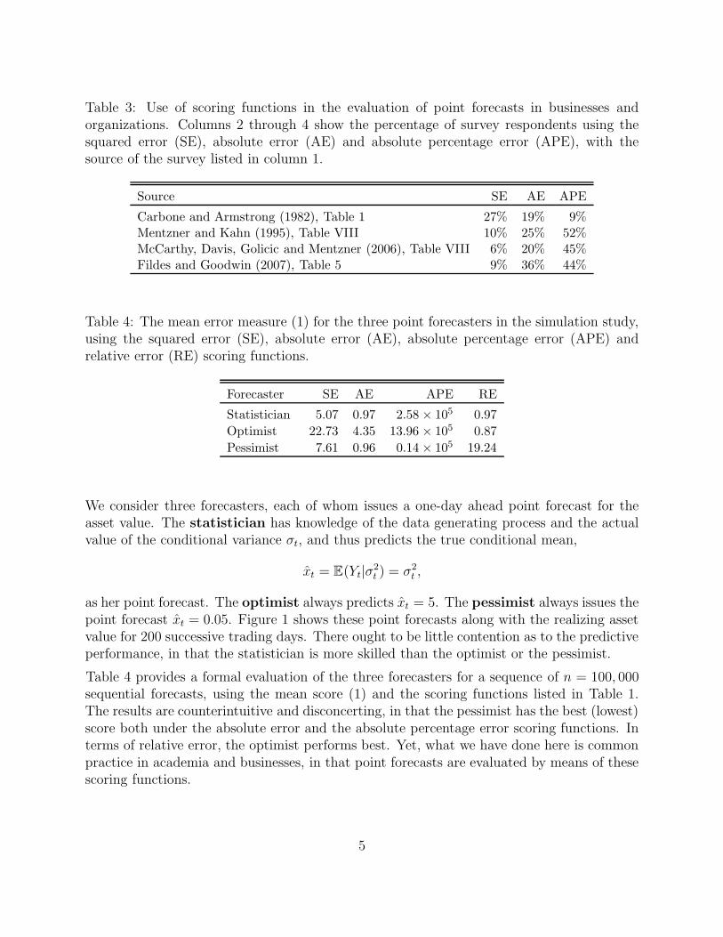
Table 3: Use of scoring functions in the evaluation of point forecasts in businesses andorganizations. Columns 2 through 4 show the percentage of survey respondents using thesquared error (SE), absolute error (AE) and absolute percentage error (APE), with thesource of the survey listed in column 1.
Source SE AE APE
Carbone and Armstrong (1982), Table 1 27% 19% 9%Mentzner and Kahn (1995), Table VIII 10% 25% 52%McCarthy, Davis, Golicic and Mentzner (2006), Table VIII 6% 20% 45%Fildes and Goodwin (2007), Table 5 9% 36% 44%
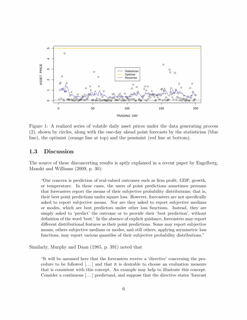
Table 4: The mean error measure (1) for the three point forecasters in the simulation study,using the squared error (SE), absolute error (AE), absolute percentage error (APE) andrelative error (RE) scoring functions.
Forecaster SE AE APE RE
Statistician 5.07 0.97 2.58 × 10⁵ 0.97
Optimist 22.73 4.35 13.96 × 10⁵ 0.87
Pessimist 7.61 0.96 0.14 × 10⁵ 19.24
We consider three forecasters, each of whom issues a one-day ahead point forecast for theasset value. The statistician has knowledge of the data generating process and the actualvalue of the conditional variance σt, and thus predicts the true conditional mean,
xt = E(Yt|σ2t ) = σ2
t ,
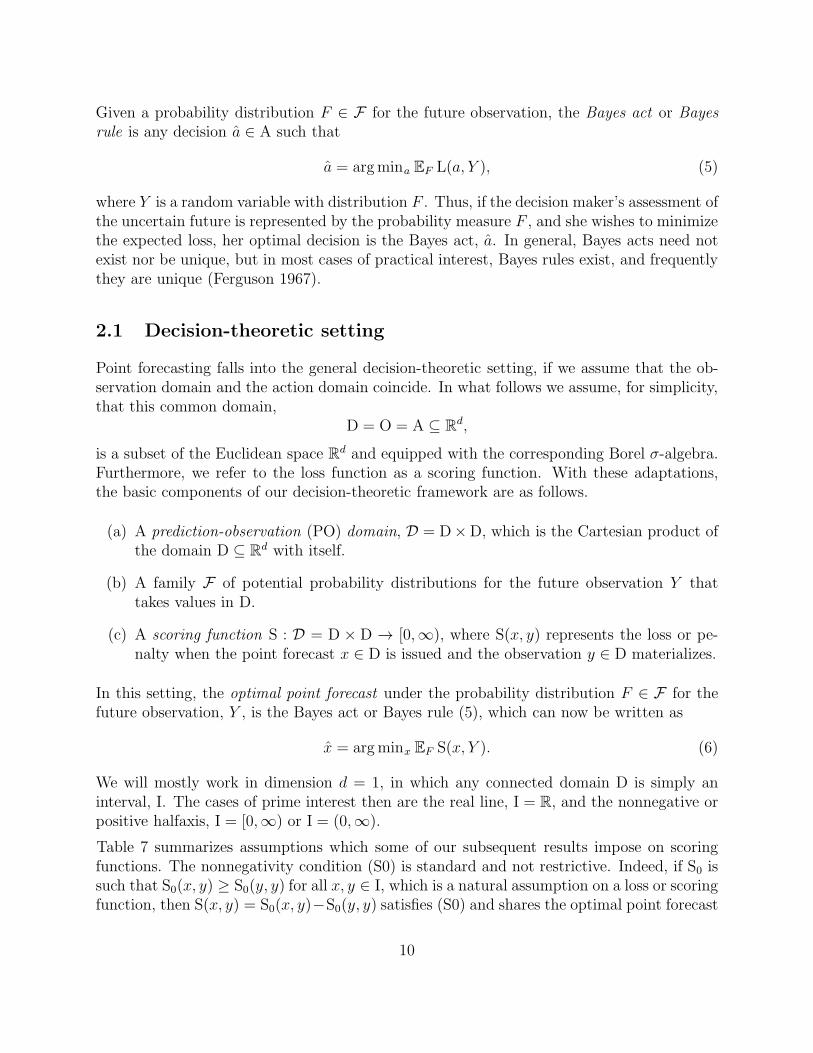
as her point forecast. The optimist always predicts xt = 5. The pessimist always issues thepoint forecast xt = 0.05. Figure 1 shows these point forecasts along with the realizing assetvalue for 200 successive trading days. There ought to be little contention as to the predictiveperformance, in that the statistician is more skilled than the optimist or the pessimist.
Table 4 provides a formal evaluation of the three forecasters for a sequence of n = 100, 000sequential forecasts, using the mean score (1) and the scoring functions listed in Table 1.The results are counterintuitive and disconcerting, in that the pessimist has the best (lowest)score both under the absolute error and the absolute percentage error scoring functions. Interms of relative error, the optimist performs best. Yet, what we have done here is commonpractice in academia and businesses, in that point forecasts are evaluated by means of thesescoring functions.
5
0 50 100 150 200
01
23
45
TRADING DAY
AS
SE
T P
RIC
E
StatisticianOptimistPessimist
Figure 1: A realized series of volatile daily asset prices under the data generating process(2), shown by circles, along with the one-day ahead point forecasts by the statistician (blueline), the optimist (orange line at top) and the pessimist (red line at bottom).
1.3 Discussion
The source of these disconcerting results is aptly explained in a recent paper by Engelberg,Manski and Williams (2009, p. 30):
“Our concern is prediction of real-valued outcomes such as firm profit, GDP, growth,or temperature. In these cases, the users of point predictions sometimes presumethat forecasters report the means of their subjective probability distributions; that is,their best point predictions under square loss. However, forecasters are not specificallyasked to report subjective means. Nor are they asked to report subjective mediansor modes, which are best predictors under other loss functions. Instead, they aresimply asked to ‘predict’ the outcome or to provide their ‘best prediction’, withoutdefinition of the word ‘best.’ In the absence of explicit guidance, forecasters may reportdifferent distributional features as their point predictions. Some may report subjectivemeans, others subjective medians or modes, and still others, applying asymmetric lossfunctions, may report various quantiles of their subjective probability distributions.”
Similarly, Murphy and Daan (1985, p. 391) noted that
“It will be assumed here that the forecasters receive a ‘directive’ concerning the pro-cedure to be followed [. . . ] and that it is desirable to choose an evaluation measurethat is consistent with this concept. An example may help to illustrate this concept.Consider a continuous [. . . ] predictand, and suppose that the directive states ‘forecast
6

the expected (or mean) value of the variable.’ In this situation, the mean square errormeasure would be an appropriate scoring rule, since it is minimized by forecasting themean of the (judgemental) probability distribution. Measures that correspond with adirective in this sense will be referred to as consistent scoring rules (for that directive).”
Despite these well-argued perspectives, there has been little recognition that the commonpractice of requesting ‘some’ point forecast, and then evaluating the forecasters by using‘some’ (set of) scoring function(s), is not a meaningful endeavor. In this paper, we developthe perspectives of Murphy and Daan (1985) and Engelberg et al. (2009) and argue thateffective point forecasting depends on ‘guidance’ or ‘directives’, which can be given in oneof two complementary ways, namely, by disclosing the scoring function ex ante to theforecaster, or by requesting a specific functional of the forecaster’s predictive distribution,such as the mean or a quantile.
As to the first option, the a priori disclosure of the scoring function allows the forecasterto tailor the point predictor to the scoring function at hand. In particular, this permitsour statistician forecaster to mutate into Mr. Bayes, who issues the optimal point forecast,namely the Bayes rule,
x = argminx EF S(x, Y ), (3)
where the expectation is taken with respect to the forecaster’s subjective or objective predic-tive distribution, F . For example, if the scoring function S is the squared error, the optimalpoint forecast is the mean of the predictive distribution. In the case of the absolute error,the Bayes rule is any median of the predictive distribution. The class
Sβ(x, y) =
∣∣∣∣1−
(y
x
)β∣∣∣∣
(β 6= 0) (4)
of scoring functions nests both the absolute percentage error (β = −1) and the relative error(β = 1) scoring functions. If the predictive distribution F has density f on the positivehalf-axis and a finite fractional moment of order β, the optimal point forecast under the lossor scoring function (4) is the median of a random variable whose density is proportional toyβf(y). We call this the β-median of the probability distribution F and write med(β)(F ).The traditional median arises in the limit as β → 0.
Table 5 summarizes our discussion, in that it shows the optimal point forecast, or Bayesrule, under the scoring functions in Table 1, both in full generality and in the special caseof the true predictive distribution under the data generating process (2). Table 6 shows themean score (1) for the new competitor Mr. Bayes in the simulation study, who issues theoptimal point forecast. As expected, Mr. Bayes outperforms his colleagues.
An alternative to disclosing the scoring function is to request a specific functional of theforecaster’s predictive distribution, such as the mean or a quantile, and to apply any scoringfunction that is consistent with the functional, roughly in the following sense.
Let the interval I be the potential range of the outcomes, such as I = R for a real-valuedquantity, or I = (0,∞) for a strictly positive quantity, and let the probability distribution F
7

Table 5: Bayes rules under the scoring functions in Table 1 as a functional of the forecaster’spredictive distribution, F . The functional med(β)(F ) is defined in the text. The final columnspecializes to the true predictive distribution under the data generating process (2) in thesimulation study. The entry for the absolute percentage error (APE) is to be understood asfollows. The predictive distribution F has infinite fractional moment of order −1, and thusmed(−1)(F ) does not exist. However, it is readily seen that the smaller the (strictly positive)point forecast, the smaller the expected APE. Thus, a prudent forecaster will issue somevery small ǫ > 0 as point predictor.
Scoring Function Bayes Rule Point Forecast in Simulation Study
SE x = mean(F ) σ2t
AE x = median(F ) 0.455σ2t
APE x = med(−1)(F ) ε
RE x = med(1)(F ) 2.366σ2t
Table 6: Continuation of Table 4, showing the corresponding mean scores for the new com-petitor, Mr. Bayes. In the case of the APE, Mr. Bayes issues the point forecast x = ǫ = 10−10.
SE AE APE RE
Mr. Bayes 5.07 0.86 1.00 0.75
be concentrated on I. Then a scoring function is any mapping S : I×I → [0,∞). A functionalis a potentially set-valued mapping F 7→ T(F ) ⊆ I. A scoring function S is consistent forthe functional T if
EF [S(t, Y )] ≤ EF [S(x, Y )]
for all F , all t ∈ T(F ) and all x ∈ I. It is strictly consistent if it is consistent and equalityof the expectations implies that x ∈ T(F ). Following Osband (1985) and Lambert, Pennockand Shoham (2008), a functional is elicitable if there exists a scoring function that is strictlyconsistent for it.
1.4 Plan of the paper
The remainder of the paper is organized as follows. Section 2 develops the notions of con-sistency and elicitability in a comprehensive way. In addition to reviewing and unifying theextant literature, we present original results on weighted scoring functions that extend priorfindings on optimal point forecasts, such as those of Park and Stefanski (1998) and Patton(2010). Section 3 turns to examples. The mean functional, ratios of expectations, quantiles
8

and expectiles are elicitable. Subject to weak regularity conditions, a scoring function for areal-valued predictand is consistent for the mean functional if and only if it is a Bregmanfunction, that is, of the form
S(x, y) = φ(y)− φ(x)− φ′(x)(y − x),
where φ is a convex function with subgradient φ′ (Savage 1971). More general and novelresults apply to ratios of expectations and expectiles. A scoring function is consistent forthe α-quantile if and only if it is generalized piecewise linear (GPL) of order α ∈ (0, 1), thatis, of the form
S(x, y) = (1(x ≥ y)− α) (g(x)− g(y)),
where 1(·) denotes an indicator function and g is nondecreasing (Thomson 1979; Saerens2000). However, not all functionals are elicitable. Notably, the conditional value-at-risk(CVaR) functional is not elicitable, despite its popularity as a risk measure in financialapplications.
The paper closes with a discussion in Section 5, which makes a plea for change in the practiceof point forecasting. I contend that in issuing and evaluating point forecasts, it is essentialthat either the scoring function be specified ex ante, or an elicitable target functional benamed, such as an expectation or a quantile, and scoring functions be used that are consistentfor the target functional.
2 A decision-theoretic approach to the evaluation of
point forecasts
We now develop a theoretical framework for the evaluation of point forecasts. Towards thisend, we review the more general, classical decision-theoretic setting whose basic ingredientsare as follows.
(a) An observation domain, O, which comprises the potential outcomes of a future obser-vation.
(b) A class F of probability measures on the observation domain O (equipped with asuitable σ-algebra), which constitutes a family of probability distributions for the futureobservation.
(c) An action domain, A, which comprises the potential actions of a decision maker.
(d) A loss function L : A×O → [0,∞), where L(a, o) represents the monetary or societalcost when the decision maker takes the action a ∈ A and the observation o ∈ Omaterializes.
9
Given a probability distribution F ∈ F for the future observation, the Bayes act or Bayesrule is any decision a ∈ A such that
a = argmina EF L(a, Y ), (5)
where Y is a random variable with distribution F . Thus, if the decision maker’s assessment ofthe uncertain future is represented by the probability measure F , and she wishes to minimizethe expected loss, her optimal decision is the Bayes act, a. In general, Bayes acts need notexist nor be unique, but in most cases of practical interest, Bayes rules exist, and frequentlythey are unique (Ferguson 1967).
2.1 Decision-theoretic setting
Point forecasting falls into the general decision-theoretic setting, if we assume that the ob-servation domain and the action domain coincide. In what follows we assume, for simplicity,that this common domain,
D = O = A ⊆ Rd,
is a subset of the Euclidean space Rd and equipped with the corresponding Borel σ-algebra.
Furthermore, we refer to the loss function as a scoring function. With these adaptations,the basic components of our decision-theoretic framework are as follows.
(a) A prediction-observation (PO) domain, D = D×D, which is the Cartesian product ofthe domain D ⊆ R
d with itself.
(b) A family F of potential probability distributions for the future observation Y thattakes values in D.
(c) A scoring function S : D = D × D → [0,∞), where S(x, y) represents the loss or pe-nalty when the point forecast x ∈ D is issued and the observation y ∈ D materializes.
In this setting, the optimal point forecast under the probability distribution F ∈ F for thefuture observation, Y , is the Bayes act or Bayes rule (5), which can now be written as
x = argminx EF S(x, Y ). (6)
We will mostly work in dimension d = 1, in which any connected domain D is simply aninterval, I. The cases of prime interest then are the real line, I = R, and the nonnegative orpositive halfaxis, I = [0,∞) or I = (0,∞).
Table 7 summarizes assumptions which some of our subsequent results impose on scoringfunctions. The nonnegativity condition (S0) is standard and not restrictive. Indeed, if S0 issuch that S0(x, y) ≥ S0(y, y) for all x, y ∈ I, which is a natural assumption on a loss or scoringfunction, then S(x, y) = S0(x, y)−S0(y, y) satisfies (S0) and shares the optimal point forecast
10

Table 7: Assumptions on a scoring function S on a PO domain D = I× I, where I ⊆ R is aninterval, x ∈ I denotes the point forecast and y ∈ I the realizing observation.
(S0) S(x, y) ≥ 0 with equality if x = y
(S1) S(x, y) is continuous in x
(S2) The partial derivative S(1)(x, y) exists and is continuous in x whenever x 6= y
(6), subject to integrability conditions that are not of practical concern. Generally, a lossfunction can be multiplied by a strictly positive constant and any function that depends on yonly can be added, without changing the nature of the optimal point forecast. Furthermore,the optimization problem in (6) is posed in terms of the point predictor, x. In this light, it isnatural that assumptions (S1) and (S2) concern continuity and differentiability with respectto the first argument, the point forecast x.
Efron (1991) and Patton (2010) argue that homogeneity or scale invariance is a desirableproperty of a scoring function. We adopt this notion and call a scoring function S on thePO domain D = D× D homogeneous of order b if
S(cx, cy) = |c|b S(x, y) for all x, y ∈ D and c ∈ R
which are such that cx ∈ D and cy ∈ D. Evidently, the underlying quest is that forequivariance in the decision problem. The scoring function S on the PO domain D = D×Dis equivariant with respect to some class H of injections h : D → D if
argminx EF [S(x, h(Y ))] = h(argminxEF [S(x, Y )])
for all h ∈ H and all probability distributions F that are concentrated on D. For instance,if S is homogeneous on D = R
d or D = (0,∞)d then it is equivariant with respect to themultiplicative group of the linear transformations x 7→ cx : c > 0. If the scoring function isof the prediction error form on D = R
d, then it is equivariant with respect to the translationgroup x 7→ x+ b : b ∈ R
d.
While our decision-theoretic setting resembles and follows those of Osband (1985) and Lam-bert et al. (2008), and the subsequent development owes much to their pioneering works,there are distinctions in technique. For example, Osband (1985) assumes a bounded domainD, while Lambert et al. (2008) consider D to be a finite set. The work of Granger andPesaran (2000a, 2000b), which argues in favor of closer links between decision theory andforecast evaluation, focuses on probability forecasts for a dichotomous event.
2.2 Consistency
In the decision-theoretic framework, we think of the aforementioned ‘distributional feature’or ‘directive’ for the forecaster as a statistical functional. Formally, a statistical functional,
11
or simply a functional, is a potentially set-valued mapping from a class of probability distri-butions, F , to a Euclidean space (Horowitz and Manski 2006; Huber and Ronchetti 2009;Wellner 2009). In the current context of point forecasting, we require that the functional
T : F −→ D, F 7−→ T(F ),
maps into the domain D ⊆ Rd. Frequently, we take F to be the class of all probability
measures on D, or the class of the probability measures with compact support in D.
To facilitate the presentation, the following definitions and results suppress the dependenceof the scoring function S, the functional T and the class F on the domain D.
Definition 2.1. The scoring function S is consistent for the functional T relative to theclass F if
EF S(t, Y ) ≤ EF S(x, Y ) (7)
for all probability distributions F ∈ F , all t ∈ T(F ) and all x ∈ D. It is strictly consistentif it is consistent and equality in (7) implies that x ∈ T(F ).
As noted, the term consistent was coined by Murphy and Daan (1985, p. 391), who stressedthat is is critically important to define consistency for a fixed, given functional, as opposed toa generic notion of consistency, which was, correctly, refuted by Jolliffe (2008). For example,the squared error scoring function, S(x, y) = (x−y)2, is consistent, but not strictly consistent,for the mean functional relative to the class of the probability measures on the real line withfinite first moment. It is strictly consistent relative to the class of the probability measureswith finite second moment.
In a parametric context, Lehmann (1951) and Noorbaloochi and Meeden (1983) refer to a re-lated property as decision-theoretic unbiasedness. The following result notes that consistencyis the dual of the optimal point forecast property, just as decision-theoretic unbiasedness isthe dual of being Bayes (Noorbaloochi and Meeden 1983). It thus connects the problems offinding optimal point forecasts, and of evaluating point predictions.
Theorem 2.2. The scoring function S is consistent for the functional T relative to the classF if and only if, given any F ∈ F , any x ∈ T(F ) is an optimal point forecast under S.
Stated differently, the class of the scoring functions that are consistent for a certain functionalis identical to the class of the loss functions under which the functional is an optimal pointforecast. Despite its simplicity, and the proof being immediate from the defining properties,this duality does not appear to be widely appreciated.
Our next result shows that the class of the consistent scoring functions is convex, and thussuggests the existence of Choquet representations (Phelps 1966).
12
Theorem 2.3. Let λ be a measure on a measurable space (Ω,A). Suppose that for allω ∈ Ω, the scoring function Sω satisfies (S0) and is consistent for the functional T relativeto the class F . Then the scoring function
S(x, y) =
∫
Sω(x, y) λ(dω)
is consistent for T relative to F .
At this point, it will be useful to distinguish the notions of a proper scoring rule (Winkler1996; Gneiting and Raftery 2007) and a consistent scoring function. I believe that thisdistinction is useful, even though the extant literature has failed to make it. For example, inreferring to proper scoring rules for quantile forecasts, Cervera and Munoz (1996), Gneitingand Raftery (2007), Hilden (2008) and Jose and Winkler (2009) discuss scoring functionsthat are consistent for a quantile.
Within our decision-theoretic framework, a proper scoring rule is a function S : F ×D → R
such thatEF S(F, Y ) ≤ EF S(G, Y ) (8)
for all probability distributions F,G ∈ F , where we assume that the expectations are well-defined. Note that S is defined on the Cartesian product of the class F and the domainD. The loss or penalty S(F, y) arises when a probabilistic forecaster issues the predictivedistribution F while y ∈ D materializes. The expectation inequality (8) then implies thatthe forecaster minimizes the expected loss by following her true beliefs. Thus, the use ofproper scoring rules encourages sincerity and candor among probabilistic forecasters.
In contrast, a scoring function S acts on the PO domain, D = D×D, that is, the Cartesianproduct of D with itself. This is a much simpler domain than that for a scoring rule. However,any consistent scoring function induces a proper scoring rule in a straightforward and naturalconstruction, as follows.
Theorem 2.4. Suppose that the scoring function S is consistent for the functional T relativeto the class F . Then the function
S : F × D −→ [0,∞), (F, y) 7−→ S(F, y) = S(T(F ), y),
is a proper scoring rule.
A more general decision-theoretic approach to the construction of proper scoring rules isdescribed by Dawid (2007, p. 78) and Gneiting and Raftery (2007, p. 361).
2.3 Elicitability
We turn to the notion of elicitability, which is a critically important concept in the evaluationof point forecasts. While the general notion dates back to the pioneering work of Osband
13
(1985), the term elicitable was coined only recently by Lambert et al. (2008). Wheneverappropriate and feasible, we suppress the dependence of the definitions and results on thePO domain D = D× D.
Definition 2.5. The functional T is elicitable relative to the class F if there exists a scoringfunction S that is strictly consistent for T relative to F .
Evidently, if T is elicitable relative to the class F , then it is elicitable relative to any subclassF0 ⊆ F . The following result then is a version of Osband’s (1985, p. 9) revelation principle.
Theorem 2.6 (Osband). Suppose that the class F is concentrated on the domain D, andlet g : D → D be a one-to-one mapping. Then the following holds.
(a) If T is elicitable, then Tg = g T is elicitable.
(b) If S is consistent for T, then the scoring function
Sg(x, y) = S(g−1(x), y)
is consistent for Tg.
(c) If S is strictly consistent for T, then Sg is strictly consistent for Tg.
The next theorem is an original result that concerns weighted scoring functions, where theweight function depends on the realizing observation, y, only.
Theorem 2.7. Let the functional T be defined on a class F of probability distributions whichadmit a density, f , with respect to some dominating measure on the domain D. Considerthe weight function
w : D → [0,∞).
Let F (w) ⊆ F denote the subclass of the probability distributions in F which are such thatw(y)f(y) has finite integral over D, and the probability measure F (w) with density propor-tional to w(y)f(y) belongs to F . Define the functional
T(w) : F (w) −→ I, F 7−→ T(w)(F ) = T(F (w)), (9)
on this subclass F (w). Then the following holds.
(a) If T is elicitable, then T(w) is elicitable.
(b) If S is consistent for T relative to F , then
S(w)(x, y) = w(y) S(x, y) (10)
is consistent for T(w) relative to F (w).
14

Table 8: The optimal point forecast or Bayes rule (6) when the scoring function is relativeerror, S(x, y) = |(x− y)/x|, and the future quantity Y can be represented as Y = Z2, whereZ has a t-distribution with mean 0, variance 1 and ν > 2 degrees of freedom. In the limitingcase as ν → ∞, we take Z to be standard normal. If Z has variance σ2 the entries need tobe multiplied by this factor. As opposed to the approximations in Table 1 of Patton (2010),which stem from numerical and Monte Carlo methods and are reproduced below, our resultsderive from Theorem 2.7 and are exact. For details see Appendix B.
ν = 4 ν = 6 ν = 8 ν = 10 ν → ∞
Exact optimal point forecast 3.4048 2.8216 2.6573 2.5801 2.3660Patton’s approximation 3.0962 2.7300 2.6067 2.5500 2.3600
(c) If S is strictly consistent for T relative to F , then S(w) is strictly consistent for T(w)
relative to F (w).
In other words, a weighted scoring function is consistent for the functional T(w), which actson the predictive distribution in a peculiar way, in that it applies the original functional,T, to the probability measure whose density is proportional to the product of the weightfunction and the original density.
Theorem 2.7 is a very general result with a wealth of applications, both in forecast evaluationand in the derivation of optimal point forecasts. In particular, the functional (9) is theoptimal point forecast under the weighted scoring function (10), which allows us to unifyand extend scattered prior results. For example, the scoring function Sβ of equation (4),
Sβ(x, y) =
∣∣∣∣1−
(y
x
)β∣∣∣∣,
is of the form (10) with the original scoring function S(x, y) = |x−β − y−β| and the weightfunction w(y) = yβ on the positive halfaxis, D = (0,∞). The scoring function S is consistentfor the median functional. Thus, as noted in the introduction, the scoring function Sβ
is consistent for the β-median functional, med(β)(F ), that is, the median of a probabilitydistribution whose density is proportional to yβf(y), where f is the density of F . If β = −1,we recover the absolute percentage error, S−1(x, y) = |(x−y)/y|. The case β = 1 correspondsto the relative error, S1(x, y) = |(x− y)/x|, which Patton (2010) refers to as the MAE-propfunction. Table 1 of Patton (2010) shows Monte Carlo based approximate values for optimalpoint forecasts under this scoring function. Theorem 2.7 permits us to give exact results;these are summarized in Table 8 and differ notably from the approximations.
Another interesting case arises when the original scoring function S is the squared error,S(x, y) = (x − y)2, which is consistent for the mean or expectation functional. If T is the
15

mean functional, the functional T(w) of equation (9) becomes
T(w)(F ) = T(F (w)) = EF (w) [Z ] =EF [Y w(Y )]
EF [w(Y )]. (11)
Park and Stefanski (1998) studied optimal point forecasts in the special case in which D =(0,∞) is the positive half-axis and w(y) = 1/y2, so that S(w)(x, y) = (x − y)2/y2 is thesquared percentage error. By equation (11), the scoring function S(w) is consistent for thefunctional T(w)(F ) = EF [Y
−1] /EF [Y−2]. By Theorem 2.2, this latter quantity is the optimal
point forecast under the squared percentage error scoring function, which is the result derivedby Park and Stefanski (1998).
Situations in which the weight function depends on the point forecast, x, need to be handledon a case-by-case basis. For example, a routine calculation shows that the squared relativeerror scoring function, S(x, y) = (x− y)2/x2, is consistent for the functional
T(F ) =EF [Y
2]
EF [Y ]. (12)
Incidentally, by a special case of (11) the observation-weighted scoring function S(x, y) =y(x− y)2 is also consistent for the functional (12). Later on in equation (23) we characterizethe class of the scoring functions that are consistent for this functional.
While Theorems 2.6 and 2.7 suggest that general classes of functionals are elicitable, not allfunctionals are such. The following result, which is a variant of Proposition 2.5 of Osband(1985) and Lemma 1 of Lambert et al. (2008), states a necessary condition.
Theorem 2.8 (Osband). If a functional is elicitable then its level sets are convex in thefollowing sense: If F0 ∈ F , F1 ∈ F and p ∈ (0, 1) are such that Fp = (1− p)F0 + pF1 ∈ F ,then t ∈ T(F0) and t ∈ T(F1) imply t ∈ T(Fp).
For example, the sum of two distinct quantiles generally does not have convex level sets andthus is not an elicitable functional. Interesting open questions include those for a converseof Theorem 2.8 and, more generally, for a characterization of elicitability.
2.4 Osband’s principle
Given an elicitable functional T, is there a practical way of describing and characterizingthe class of the scoring functions that are consistent for it? The following general approach,which originates in the pioneering work of Osband (1985), is frequently useful.
Suppose that the functional T is defined for a class of probability measures on the domainD which includes the two-point distributions. Assume that there exists an identificationfunction V : D×D → R such that
EF [V(x, Y )] = 0 ⇐⇒ x ∈ T(F ) (13)
16

Table 9: Possible choices for the identification function V with the property (13) in the casein which D = I ⊆ R is an interval.
Functional Identification function
Mean V(x, y) = x− yRatio EF [r(Y )] /EF [s(Y )] V(x, y) = xs(y)− r(y)α-Quantile V(x, y) = 1(x ≥ y)− ατ -Expectile V(x, y) = 2 |1(x ≥ y)− τ | (x− y)
and V(x, y) 6= 0 unless x = y. If a consistent scoring function is available, which is smoothin its first argument, we can take V(x, y) to be the corresponding partial derivative. Forexample, if T is the mean or expectation functional on an interval D = I ⊆ R, we can pickV(x, y) = x − y, which derives from the squared error scoring function, S(x, y) = (x − y)2.Table 9 provides further examples, with the second and fourth nesting the first.
The functionǫ(c) = p S(c, a) + (1− p)S(c, b) (14)
represents the expected score when we issue the point forecast c for a random vector Y suchthat Y = a with probability p and Y = b with probability 1 − p. Since S is consistent forthe functional T, the identification function property (13) implies that ǫ(c) has a minimumat c = x, where
pV(x, a) + (1− p) V(x, b) = 0. (15)
If S is smooth in its first argument, we can combine (14) and (15) to result in
S(1)(x, a)/V(x, a) = S(1)(x, b)/V(x, b), (16)
where S(1) denotes a partial derivative or gradient with respect to the first argument. If thislatter equality holds for all pairwise distinct a, b and x ∈ D, the function S(1)(x, y)/V(x, y)is independent of y ∈ D, and we can write
S(1)(x, y) = h(x) V(x, y) (17)
for x, y ∈ D and some function h : D → D. Frequently, we can integrate (17) to obtain thegeneral form of a scoring rule that is consistent for the functional T.
In recognition of Osband’s (1985) fundamental yet unpublished work, we refer to this gen-eral approach as Osband’s principle. The examples in the subsequent section give variousinstances in which the principle can be successfully put to work. For a general technicalresult, see Theorem 2.1 of Osband (1985).
17

3 Examples
We now give examples in the case of a univariate predictand, in which any connected domainD = I ⊆ R is an interval. Some of the results are classical, such as the characterizationsfor expectations (Savage 1971) and quantiles (Thomson 1979), and some are novel, includ-ing those for ratios of expectations, expectiles and conditional value-at-risk. In a majorityof the examples, the technical arguments rely on the properties of convex functions andsubgradients, for which we refer to Rockafellar (1970).
3.1 Expectations
It is well known that the squared error scoring function, S(x, y) = (x − y)2, is strictlyconsistent for the mean functional relative to the class of the probability distributions on R
whose second moment is finite. Thus, means or expectations are elicitable. Before turningto more general settings in subsequent sections, we review a classical result of Savage (1971)which identifies the class of the scoring functions that are consistent for the mean functionalas that of the Bregman functions. Closely related results have been obtained by Reichelsteinand Osband (1984), Saerens (2000), Banerjee, Guo and Wang (2005) and Patton (2010).
Theorem 3.1 (Savage). Let F be the class of the probability measures on the interval I ⊆ R
with finite first moment. Then the following holds.
(a) The mean functional is elicitable relative to the class F .
(b) Suppose that the scoring function S satisfies assumptions (S0), (S1) and (S2) on thePO domain D = I × I. Then S is consistent for the mean functional relative to theclass of the compactly supported probability measures on I if, and only if, it is of theform
S(x, y) = φ(y)− φ(x)− φ′(x)(y − x), (18)
where φ is a convex function with subgradient φ′ on I.
(c) If φ is strictly convex, the scoring function (18) is strictly consistent for the meanfunctional relative to the class of the probability measures F on I for which both EF Yand EF φ(Y ) exist and are finite.
Banerjee et al. (2005) refer to a function of the form (18) as a Bregman function. Forexample, if I = R and φ(x) = |x|a, where a > 1 to ensure strict convexity, the Bregmanrepresentation yields the scoring function
Sa(x, y) = |y|a − |x|a − a sign(x)|x|a−1(y − x), (19)
which is homogeneous of order a and nests the squared error that arises when a = 2. Savage(1971) showed that up to a multiplicative constant squared error is the unique Bregman
18

−0.5 0.0 0.5 1.0 1.5 2.0 2.5
05
1015
PATTON PARAMETER B
ME
AN
SC
OR
E
Mr BayesOptimistPessimist
Figure 2: The mean score (1) under the Patton scoring function (20) for Mr. Bayes (green),the optimist (orange) and the pessimist (red) in the simulation study of Section 1.2.
function of the prediction error form, as well as the unique symmetric Bregman function.Patton (2010) introduced a rich and flexible family of homogeneous Bregman functions onthe PO domain D = (0,∞)× (0,∞), namely
Sb(x, y) =
1
b(b− 1)
(yb − xb
)−
1
b− 1xb−1 (y − x) if b ∈ R \ 0, 1,
y
x− log
y
x− 1 if b = 0,
y logy
x− y + x if b = 1.
(20)
Up to a multiplicative constant, these are the only homogeneous Bregman functions onthis PO domain. The squared error scoring function emerges when b = 2 and the QLIKEfunction (Patton 2010) when b = 0. If b = a > 1 the Patton function (20) coincides with thecorresponding restriction of the power function (19), up to a multiplicative constant.
Finally, it is worth noting that roper scoring rules for probability forecasts of a dichotomousevent are also of the Bregman form, because the probability of a binary event equals theexpectation of the corresponding indicator variable. Compare McCarthy (1956), Savage(1971), DeGroot and Fienberg (1983), Schervish (1989), Winkler (1996), Buja, Stuetzle andShen (2005) and Gneiting and Raftery (2007), among others.
Figure 2 returns to the initial simulation study of Section 1.2 and shows the mean score(1) under the Patton scoring function (20) for Mr. Bayes, the optimist and the pessimist.
19

The optimal point forecast under a Bregman scoring function is the mean of the predictivedistribution, so that the statistician forecaster fuses with Mr. Bayes.
3.2 Ratios of expectations
We now consider statistical functionals which can be represented as ratios of expectations.The mean functional emerges in the special case in which r(y) = y and s(y) = 1.
Theorem 3.2. Let I ⊆ R be an interval, and suppose that r : I → R and s : I → (0,∞) aremeasurable functions. Then the following holds.
(a) The functional
T(F ) =EF [r(Y )]
EF [s(Y )](21)
is elicitable relative to the class of the probability measures on I for which EF [r(Y )],EF [s(Y )] and EF [Y s(Y )] exist and are finite.
(b) If S is of the form
S(x, y) = s(y) (φ(y)− φ(x))− φ′(x)(r(y)− xs(y)) + φ′(y)(r(y)− ys(y)), (22)
where φ is a convex function with subgradient φ′, then it is consistent for the func-tional (21) relative to the class of the probability measures F on I for which EF [r(Y )],EF [s(Y )], EF [r(Y )φ′(Y )], EF [s(Y )φ(Y )] and EF [Y s(Y )φ′(Y )] exist and are finite. Ifφ is strictly convex, then S is strictly consistent.
(c) Suppose that the scoring function S satisfies assumptions (S0), (S1) and (S2) on thePO domain D = I × I. If s is continuous and r(y) = ys(y) for y ∈ I, then Sis consistent for the functional (21) relative to the class of the compactly supportedprobability measures on I if, and only if, it is of the form (22), where φ is a convexfunction with subgradient φ′.
In the case in which s(y) = w(y) and r(y) = yw(y) for a strictly positive, continuous weightfunction w, the ratio (21) coincides with the functional (11). If I = (0,∞) and w(y) = y,the special case T(F ) = EF [Y
2] /EF [Y ] of equation (12) arises. In Section 2.3 we saw thatboth the squared relative error scoring function, S(x, y) = (x− y)2/x2, and the observation-weighted scoring function S(x, y) = y(x− y)2 are consistent for this functional. By part (c)of Theorem 3.2, the general form of a scoring function that is consistent for the functional(12) is
S(x, y) = y (φ(y)− φ(x))− y (y − x)φ′(x), (23)
where φ is convex with subgradient φ′. The above scoring functions emerge when φ(y) = 1/yand φ(y) = y2, respectively.
20

3.3 Quantiles and expectiles
An α-quantile (0 < α < 1) of the cumulative distribution function F is any number x forwhich limy↑x F (y) ≤ α ≤ F (x). In finance, quantiles are often referred to as value-at-risk(VaR; Duffie and Pan 1997). The literature on the evaluation of quantile forecasts generallyrecommends the use of the asymmetric piecewise linear scoring function,
Sα(x, y) = (1(x ≥ y)− α) (x− y), (24)
which is strictly consistent for the α-quantile relative to the class of the probability measureswith finite first moment (Raiffa and Schlaifer 1961, p. 196; Ferguson 1967, p. 51). This well-known property lies at the heart of quantile regression (Koenker and Bassett 1978).
As regards the characterization of the scoring functions that are consistent for a quantile,results of Thomson (1979) and Saerens (2000) can be summarized as follows. For a discussionof their equivalence and historical comments, see Gneiting (2010).
Theorem 3.3 (Thomson, Saerens). Let F be the class of the probability measures on theinterval I ⊆ R, and let α ∈ (0, 1). Then the following holds.
(a) The α-quantile functional is elicitable relative to the class F .
(b) Suppose that the scoring function S satisfies assumptions (S0), (S1) and (S2) on thePO domain D = I× I. Then S is consistent for the α-quantile relative to the class ofthe compactly supported probability measures on I if, and only if, it is of the form
S(x, y) = (1(x ≥ y)− α) ( g(x)− g(y)), (25)
where g is a nondecreasing function on I.
(c) If g is strictly increasing, the scoring function (25) is strictly consistent for the α-quantile relative to the class of the probability measures F on I for which EF g(Y )exists and is finite.
Gneiting (2008b) refers to a function of the form (25) as generalized piecewise linear (GPL)of order α ∈ (0, 1), because it is piecewise linear after applying a nondecreasing transfor-mation. Any GPL function is equivariant with respect to the class of the nondecreasingtransformations, just as the quantile functional is equivariant under monotone mappings(Koenker 2005, p. 39). If I = (0,∞) and g(x) = xb/|b| for b ∈ R \ 0, and taking thecorresponding limit as b → 0, we obtain the family
Sα,b(x, y) =
(1(x ≥ y)− α)1
|b|
(xb − yb
)if b ∈ R \ 0,
(1(x ≥ y)− α) logx
yif b = 0,
(26)
21
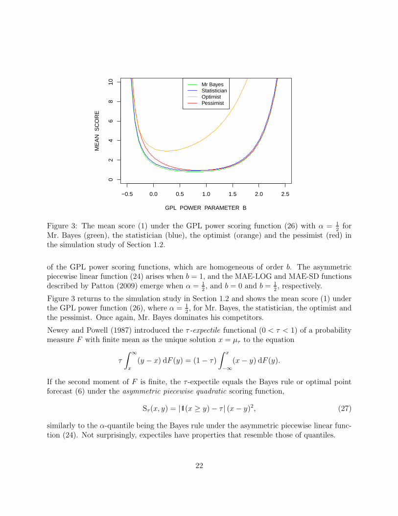
−0.5 0.0 0.5 1.0 1.5 2.0 2.5
02
46
810
GPL POWER PARAMETER B
ME
AN
SC
OR
E
Mr BayesStatisticianOptimistPessimist
Figure 3: The mean score (1) under the GPL power scoring function (26) with α = 12for
Mr. Bayes (green), the statistician (blue), the optimist (orange) and the pessimist (red) inthe simulation study of Section 1.2.
of the GPL power scoring functions, which are homogeneous of order b. The asymmetricpiecewise linear function (24) arises when b = 1, and the MAE-LOG and MAE-SD functionsdescribed by Patton (2009) emerge when α = 1
2, and b = 0 and b = 1
2, respectively.
Figure 3 returns to the simulation study in Section 1.2 and shows the mean score (1) underthe GPL power function (26), where α = 1
2, for Mr. Bayes, the statistician, the optimist and
the pessimist. Once again, Mr. Bayes dominates his competitors.
Newey and Powell (1987) introduced the τ -expectile functional (0 < τ < 1) of a probabilitymeasure F with finite mean as the unique solution x = µτ to the equation
τ
∫ ∞
x
(y − x) dF (y) = (1− τ)
∫ x
−∞
(x− y) dF (y).
If the second moment of F is finite, the τ -expectile equals the Bayes rule or optimal pointforecast (6) under the asymmetric piecewise quadratic scoring function,
Sτ (x, y) = |1(x ≥ y)− τ | (x− y)2, (27)
similarly to the α-quantile being the Bayes rule under the asymmetric piecewise linear func-tion (24). Not surprisingly, expectiles have properties that resemble those of quantiles.
22
The following original result characterizes the class of the scoring functions that are consistentfor expectiles. It is interesting to observe the ways in which the corresponding class (28)combines key characteristics of the Bregman and GPL families.
Theorem 3.4. Let F be the class of the probability measures on the interval I ⊆ R withfinite first moment, and let τ ∈ (0, 1). Then the following holds.
(a) The τ -expectile functional is elicitable relative to the class F .
(b) Suppose that the scoring function S satisfies assumptions (S0), (S1) and (S2) on thePO domain D = I× I. Then S is consistent for the τ -expectile relative to the class ofthe compactly supported probability measures on I if, and only if, it is of the form
S(x, y) = |1(x ≥ y)− τ | (φ(y)− φ(x)− φ′(x)(y − x)) , (28)
where φ is a convex function with subgradient φ′ on I.
(c) If φ is strictly convex, the scoring function (28) is strictly consistent for the τ -expectilerelative to the class of the probability measures F on I for which both EF Y and EF φ(Y )exist and are finite.
3.4 Conditional value-at-risk
The α-conditional value-at-risk functional (CVaRα, 0 < α < 1) equals the expectation of arandom variable with distribution F conditional on it taking values in its upper (1− α)-tail(Rockafellar and Uryasev 2000, 2002). An often convenient, equivalent definition is
CVaRα(F ) =1
1− α
∫ 1
α
qβ(F ) dβ, (29)
where qβ denotes the β-quantile (Acerbi 2002), similarly to the functional representationof the α-trimmed mean (Huber and Ronchetti 2009). The CVaR functional is a popularrisk measure in quantitative finance. Its varied, elegant and appealing properties includecoherency in the sense of Artzner et al. (1999), who consider functionals defined in terms ofrandom variables, rather than the corresponding probability measures.
Theorem 3.5. The CVaRα functional is not elicitable relative to any class F of probabilitydistributions on the interval I ⊆ R that contains the measures with finite support, or thefinite mixtures of the absolutely continuous distributions with compact support.
This negative result challenges the use of the CVaR functional as a predictive measure of risk,and may provide a partial explanation for the striking lack of literature on the evaluation ofCVaR forecasts, as opposed to quantile or VaR forecasts, for which we refer to Berkowitz andO’Brien (2002), Giacomini and Komunjer (2005) and Bao, Lee and Saltoglu (2006), amongothers. With consistent scoring functions not being available, it remains unclear how onemight assess and compare CVaR forecasts.
23

3.5 Mode
Let F be a class of probability measures on the real line, each of which has a well-defined,unique mode. It is sometimes stated informally that the mode is an optimal point forecastunder the zero-one scoring function,
Sc(x, y) = 1(|x− y| > c),
where c > 0. A rigorous statement is that the optimal point forecast or Bayes rule (6) underthe scoring function Sc is the midpoint
x = argmax x (F (x+ c)− limy↑x−cF (y))
of the modal interval of length 2c of the probability measure F ∈ F (Ferguson 1967, p. 51).Example 7.20 of Lehmann and Casella (1998) explores this argument in more detail.
Expressed differently, the zero-one scoring function Sc is consistent for the midpoint func-tional, which we denote by Tc. If c is sufficiently small, then Tc(F ) is well-defined andsingle-valued for all F ∈ F . We can then define the mode functional on F as the limit
T0(F ) = limc↓0Tc(F ).
I do not know whether or not T0 is elicitable. However, if the members of the class F havecontinuous Lebesgue densities, then T0 is asymptotically elicitable, in the sense that it canbe represented as the continuous limit of a family of elicitable functionals.
Stronger results become available if one puts conditions on both the scoring function S andthe family F of probability distributions. Theorem 2 of Granger (1969) is a result of thistype. Consider the PO domain D = R×R. If the scoring function S is an even function of theprediction error that attains a minimum at the origin, and each F ∈ F admits a Lebesguedensity, f , which is symmetric, continuous and unimodal, so that mean, median and modecoincide, then S is consistent for this common functional. Theorem 1 of Granger (1969)and Theorem 7.15 of Lehmann and Casella (1998) trade the continuity and unimodalityconditions on f for an additional assumption of convexity on the scoring function.
Henderson, Jones and Stare (2001, p. 3087) posit that in survival analysis a loss function ofthe form
S∗k(x, y) =
0,x
k≤ y ≤ kx
1, otherwise
= 1(| log(x)− log(y)| > log(k))
is reasonable, with a choice of k = 2 often being adequate, arguing that “most people forexample would accept that a lifetime prediction of, say, 2 months, was reasonably accurate ifdeath occurs between about 1 and 4 months”. From the above, the optimal point forecast orBayes rule under S∗
k is the midpoint functional Tlog(k) applied to the predictive distributionof the logarithm of the lifetime, rather than the lifetime itself. Henderson et al. (2001) givevarious examples.
24

4 Multivariate predictands
While thus far we have restricted attention to point forecasts of a univariate quantity, thegeneral case of a multivariate predictand that takes values in a domain D ⊆ R
d is of consid-erable interest. Applications include those of Gneiting et al. (2008) and Hering and Genton(2010) to predictions of wind vectors, or that of Laurent, Rombouts and Violante (2009)to forecasts of multivariate volatility, to name but a few. We turn to the decision-theoreticsetting of Section 2.1 and assume, for simplicity, that the point forecast, the observation andthe target functional take values in D = R
d.
We first discuss the mean functional. Assuming that S(x, y) ≥ 0 with equality if x = y,Savage (1971), Osband and Reichelstein (1985) and Banerjee et al. (2005) showed that ascoring function under which the (component-wise) expectation of the predictive distributionis an optimal point forecast, is of the Bregman form
S(x, y) = φ(y)− φ(x)− 〈∇φ(x), y − x〉, (30)
where φ : Rd → R is convex with gradient ∇φ : Rd → Rd and 〈 , 〉 denotes a scalar prod-
uct, subject to smoothness conditions. Expressed differently, a sufficiently smooth scoringfunction is consistent for the mean functional if and only if it is of the form (30), which isa generalization of the Bregman representation (18) in the case of a univariate predictand.When φ(x) = ‖x‖2 is the squared Euclidean norm, we obtain the squared error scoringfunction, and similarly its ramifications, such as the weighted squared error and the pseudoMahalanobis error (Laurent et al. 2009).
It is of interest to note that rigorous versions of the Bregman characterization depend onrestrictive smoothness conditions. Osband and Reichelstein (1985) assume that the scoringfunction is continuously differentiable with respect to its first argument, the point forecast;Banerjee et al. (2005) assume the existence of continuous second partial derivatives withrespect to the observation. A challenging, nontrivial problem is to unify and strengthenthese results, both in univariate and multivariate settings.
Laurent et al. (2009) consider point forecasts of multivariate stochastic volatility, where thepredictand is a symmetric and positive definite matrix in R
q×q. If the matrix is vectorized, theabove results for the mean functional apply, thereby leading to the Bregman representation(30) for the respective consistent scoring functions, which is hidden in Proposition 3 ofLaurent et al. (2009). Corollary 1 of Laurent et al. (2009) supplies a version thereof thatapplies directly to point forecasts, say Σx ∈ R
q×q, of a matrix-valued, symmetric and positivedefinite quantity, say Σy ∈ R
q×q, without any need to resort to vectorization. Specifically,any scoring function of the form
S(Σx,Σy) = φ(Σy)− φ(Σx)− tr (∇0 φ(Σx)(Σy − Σx)) (31)
is consistent for the (component-wise) mean functional, where φ is convex and smooth, and∇0 φ denotes a symmetric matrix of first partial derivatives, with the off-diagonal elementsmultiplied by a factor of one half.
25
Dawid and Sebastiani (1999) and Pukelsheim (2006) give various examples of convex func-tions φ whose domain is the cone of the symmetric and positive definite elements of Rq×q,with the matrix norm
φ(Σ) =
(1
qtr(Σs)
)1/s
(32)
for s > 1 being one such instance. The matrix norm is nonnegative, nondecreasing inthe Loewner order, continuous, strictly convex, standardized and homogeneous of orderone. With simple adaptations, the construction extends to any real or extended real-valuedexponent s and to general, not necessarily positive definite symmetric matrices (Pukelsheim2006, pp. 141 and 151). In the limit as s → 0 in (32) the log determinant φ(Σ) = log det(Σ)emerges. When used in the Bregman representation (31), the log determinant function givesrise to a well known homogeneous scoring function for point predictions of a positive definitesymmetrically matrix-valued quantity in R
q×q, namely,
S(Σx,Σy) = tr(Σ−1
x Σy
)− log det
(Σ−1
x Σy
)− q, (33)
which was introduced by James and Stein (1961, Section 5). When q = 1 the scoring function(33) reduces to the Patton function (20) with b = 0, that is, the QLIKE function.
In the case of quantiles, the passage from the univariate functional to multivariate analoguesis much less straightforward. Notions of quantiles for multivariate distributions based onloss or scoring functions have been studied by Abdous and Theodorescu (1992), Chaudhuri(1996), Koltchinskii (1997), Serfling (2002) and Hallin, Paindaveine and Siman (2010), amongothers. In particular, it is customary to define the median of a probability distribution F onR
d asx = argminx EF (‖x− Y ‖ − ‖Y ‖),
where ‖ · ‖ denotes the Euclidean norm (Small 1990). If d = 1, this yields the traditionalmedian on the real line, with the ‖Y ‖ term eliminating the need for moment conditions onthe predictive distribution (Kemperman 1987). Of course, norms and distances other thanthe Euclidean could be considered. In this more general type of situation, Koenker (2006)proposed that a functional based on minimizing the square of a distance be called a Frechetmean, and a functional based on minimizing a distance a Frechet median, just as in thetraditional case of the Euclidean distance.
5 Discussion
Ideally, forecasts ought to be probabilistic, taking the form of predictive distributions overfuture quantities and events (Dawid 1984; Diebold et al. 1998; Granger and Pesaran 2000a,2000b; Gneiting 2008a). If point forecasts are to be issued and evaluated, it is essential thateither the scoring function be specified ex ante, or an elicitable target functional be named,such as the mean or a quantile of the predictive distribution, and scoring functions be usedthat are consistent for the target functional.
26

Our plea for the use of consistent scoring functions supplements and qualifies, but does notcontradict, extant recommendations in the forecasting literature, such as those of Armstrong(2001), Jolliffe and Stephenson (2003) and Fildes and Goodwin (2007). For example, Fildesand Goodwin (2007) propose forecasting principles for organizations, the eleventh of whichsuggests that “multiple measures of forecast accuracy” be employed. I agree, with thequalification that the scoring functions to be used be consistent for the target functional.
We have developed theory for the notions of consistency and elicitability, and have char-acterized the classes of the loss or scoring functions that result in expectations, ratios ofexpectations, quantiles or expectiles as optimal point forecasts. Some of these results areclassical, such as those for means and quantiles (Savage 1971; Thomson 1979), while othersare original, including a disconcerting negative result, in that scoring functions which areconsistent for the CVaR functional do not exist.
In the case of the mean functional, the consistent scoring functions are the Bregman functionsof the form (18). Among these, a particularly attractive choice is the Patton family (20) ofhomogeneous scoring functions, which nests the squared error (SE) and QLIKE functions.In evaluating volatility forecasts, Patton and Sheppard (2009) recommend the use of thelatter because of its superior power in Diebold and Mariano (1995) and West (1996) tests ofpredictive ability, which depend on differences between mean scores of the form (1) as teststatistics. Further work in this direction is desirable, both empirically and theoretically. Ifquantile forecasts are to be assessed, the consistent scoring functions are the GPL functionsof the form (25), with the homogeneous power functions in (26) being appealing examples.Interestingly, the scoring functions that are consistent for expectiles combine key elementsof the Bregman and GPL families.
As regards the most commonly used scoring functions in academia, businesses and organi-zations, the squared error scoring function is consistent for the mean, and the absolute errorscoring function for the median. The absolute percentage error scoring function, which iscommonly used by businesses and organizations, and occasionally in academia, is consistentfor a non-standard functional, namely, the median of order −1, med(−1), which tends to sup-port severe underforecasts, as compared to the mean or median. It thus seems prudent thatbusinesses and organizations consider the intended or unintended consequences and reassessits suitability as a scoring function.
Pers et al. (2009) propose a game of prediction for a fair comparison between competingpredictive models, which employs proper scoring rules. As Theorem 2.4 shows, consistentscoring functions can be interpreted as proper scoring rules. Hence, the protocol of Pers etal. (2009) applies directly to the evaluation of point forecasting methods. Their focus is onthe comparison of custom-built predictive models for a specific purpose, as opposed to theM-competitions in the forecasting literature (Makridakis and Hibon 1979, 2000; Makridakiset al. 1982, 1993), which compare the predictive performance of point forecasting methodsacross multiple, unrelated time series. In this latter context, additional considerations arise,such as the comparability of scores across time series with realizations of differing magnitudeand volatility, and commonly used evaluation methods remains controversial (Armstrong and
27
Collopy 1992; Fildes 1992; Ahlburg et al. 1992; Hyndman and Koehler 2006).
The notions of consistency and elicitability apply to point forecast competitions, whereparticipants ought to be advised ex ante about the scoring function(s) to be employed,or, alternatively, target functional(s) ought to be named. If multiple target functionalsare named, participants can enter possibly distinct point forecasts for distinct functionals.Similarly, if multiple scoring functions are to be used in the evaluation, and the scoringfunctions are consistent for distinct functionals, participants ought to be allowed to submitpossibly distinct point forecasts.
While thus far we have addressed forecasting or prediction problems, similar issues arisewhen the goal is estimation. Technically, our discussion relates to M-estimation (Huber1964; Huber and Ronchetti 2009). A century ago Keynes (1911, p. 325) derived the Breg-man representation (18) in characterizing the probability density functions for which the“most probable value” is the arithmetic mean. For a contemporary perspective in termsof maximum likelihood and M-estimation, see Klein and Grottke (2008). Komunjer (2005)applied the GPL class (25) in conditional quantile estimation, in generalization of the tra-ditional approach to quantile regression, which is based on the asymmetric piecewise linearscoring function (Koenker and Bassett 1978). Similarly, Bregman functions of the origi-nal form (18) and of the variant in (28) could be employed in generalizing symmetric andasymmetric least squares regression.
In applied settings, the distinction between prediction and estimation is frequently blurred.For example, Shipp and Cohen (2009) report on U.S. Census Bureau plans for evaluatingpopulation estimates against the results of the 2010 Census. Five measures of accuracy areto be used to assess the Census Bureau estimates, including the root mean squared error(SE) and the mean absolute percentage error (APE). Our results demonstrate that CensusBureau scientists face an impossible task in designing procedures and point estimates aimedat minimizing both measures simultaneously, because the SE and the APE are consistent fordistinct statistical functionals. In this light, it may be desirable for administrative or politicalleadership to provide a directive or target functional to Census Bureau scientists, much inthe way that Murphy and Daan (1985) and Engelberg et al. (2009) requested guidance forpoint forecasters, in the quotes that open and motivate this paper.
Appendix A: Proofs
Proof of Theorem 2.3. Given F ∈ F , let t ∈ T(F ) and x ∈ D. Then
EF S(t, Y ) = EF
[ ∫
Sω(t, y) λ(dω)
]
=
∫ [
EF Sω(t, y)]
λ(dω)
≤
∫ [
EF Sω(x, y)]
λ(dω) = EF S(x, Y ),
28
where the interchange of the expectation and the integration is allowable, because each Sω
is a nonnegative scoring function.
Proof of Theorem 2.4. Given any two probability measures F,G ∈ F , we have
EF S(F, Y ) = EF S(T(F ), Y ) ≤ EF S(T(G), Y ) = EF S(G, Y ),
where the expectations are well-defined, because the scoring function S is nonnegative.
Proof of Theorem 2.6. We first show part (b). Towards this end, let tg ∈ Tg(F ) and xg ∈ D.Then tg = g(t) for some t ∈ T(F ) and xg = g(x) for some x ∈ D. Therefore,
EF Sg(tg, Y ) = EF S(t, Y ) ≤ EF S(x, Y ) = EF Sg(xg, Y ).
As regards parts (c) and (a), it suffices to note that if S is strictly consistent, we have equalityif and only if x ∈ T(F ) or, equivalently, xg ∈ Tg(F ).
Proof of Theorem 2.7. We first prove part (b). Let F ∈ F (w), t ∈ T(w)(F ) and x ∈ D. Then
EF S(w)(t, Y ) = EF [w(Y ) S(t, Y )]
=
∫
S(t, y)w(y)f(y) µ(dy)
=
[ ∫
S(t, y) dF (w)(y)
]
·
[ ∫
w(y)f(y) µ(dy)
]−1
≤
[ ∫
S(x, y) dF (w)(y)
]
·
[ ∫
w(y)f(y) µ(dy)
]−1
= EF [w(Y ) S(x, Y )]
= EF
[
S(w)(x, Y )]
,
where µ is a dominating measure. The critical inequality holds because F (w) ∈ F (w) ⊆ Fand t(w) ∈ T(w)(F ) = T(F (w)). To prove parts (c) and (a), we note that the inequality isstrict if S is strictly consistent for S, unless x ∈ T(F (w)) = T(w)(F ).
Proof of Theorem 2.8. Suppose that the functional T is elicitable relative to the class Fon the domain D. Then there exists a scoring function S which is strictly consistent for itrelative to F . Suppose now that F0 ∈ F , F1 ∈ F and t ∈ D are such that t ∈ T(F0) andt ∈ T(F1). If x ∈ D is arbitrary and p ∈ (0, 1) is such that Fp = (1− p)F0 + pF1 ∈ F then
EFpS(t, Y ) = (1− p)EF0S(t, Y ) + pEF1S(t, Y )
≤ (1− p)EF0S(x, Y ) + pEF1S(x, Y ) = EFpS(x, Y ).
29

Hence, t ∈ T(Fp).
Sketch of the proof of Theorem 3.1. The statements in parts (b) and (c) are immediate fromthe arguments in Section 6.3 of Savage (1971), and form special cases of the more generalresult in Theorem 3.2. To prove the necessity of the representation (18), Savage essentiallyapplied Osband’s principle with the identification function V(x, y) = x− y.
Proof of Theorem 3.2. We first prove part (b). To show the sufficiency of the representation(22), let x ∈ I and let F be a probability measure on I for which EF [r(Y )], EF [s(Y )],EF [r(Y )φ′(Y )], EF [s(Y )φ(Y )] and EF [Y s(Y )φ′(Y )] exist and are finite. Then
EF S(x, Y )− EF S
(EF [r(Y )]
EF [s(Y )], Y
)
= EF [s(Y )]
φ
(EF [r(Y )]
EF [s(Y )]
)
− φ(x)− φ′(x)
(EF [r(Y )]
EF [s(Y )]− x
)
is nonnegative, and is strictly positive if φ is strictly convex and x 6= EF [r(Y )] /EF [s(Y )].
As regards part (c), it remains to show the necessity of the representation (22). We applyOsband’s principle with the identification function V(x, y) = xs(y) − r(y), as proposed byOsband (1985, p. 14). Arguing in the same way as in Section 2.4, we see that
S(1)(x, a)/(xs(a)− r(a)) = S(1)(x, b)/(xs(b)− r(b))
for all pairwise distinct a, b and x ∈ I. Hence,
S(1)(x, y) = h(x)(xs(y)− r(y))
for x, y ∈ I and some function h : I → I. Partial integration yields the representation (22),where
φ(x) =
∫ x
x0
∫ s
x0
h(u) du ds (34)
for some x0 ∈ I. Finally, φ is convex, because the scoring function S is nonnegative, whichimplies the validity of the subgradient inequality.
To prove part (a), we consider the scoring function (22) with φ(y) = y2/(1 + |y|), for whichthe expectations in part (b) exist and are finite if, and only if, EF [r(Y )], EF [s(Y )] andEF [Y s(Y )] exist and are finite.
Sketch of the proof of Theorem 3.3. For concise yet full-fledged proofs of parts (b) and (c),see Gneiting (2008b), where Osband’s principle is applied with the identification functionV(x, y) = 1(x ≥ y)−α. To prove part (a), we may apply part (c) with any strictly increasing,bounded function g : I → I, with g(x) = exp(−x)/(1+ exp(−x)) being one such example.
30

Proof of Theorem 3.4. To show the sufficiency of the representation (28), let x ∈ I wherex < µτ , and let F be a probability measure with compact support in I. A tedious butstraightforward calculation shows that if S is of the form (28) then
EF S(x, Y )− EF S(µτ , Y )
= (1− τ)
∫
(−∞, x)
(φ(µτ)− φ(x)− φ′(x)(µτ − x)) dF (y)
+ τ
∫
[x,µτ )
(φ(y)− φ(x)− φ′(x)(y − x)) dF (y)
+ τ
∫
[µτ ,∞)
(φ(µτ)− φ(x)− φ′(x)(µτ − x)) dF (y)
+ (1− τ)
∫
[x, µτ )
(φ(µτ )− φ(y)− φ′(x)(µτ − y))︸ ︷︷ ︸
≥ φ(µτ )−φ(y)−φ′(y)(µτ−y) ≥ 0
dF (y)
is nonnegative, and is strictly positive if φ is strictly convex. An analogous argument applieswhen x > µτ . This proves sufficiency in part (b) as well as the claim in part (c).
To prove the necessity of the representation (28) in part (b), we apply Osband’s principlewith the identification function V(x, y) = |1(x ≥ y)− τ | (x− y). Arguing in the usual way,we see that
S(1)(x, y) = h(x) V (x, y)
for x, y ∈ I and some function h : I → I. Partial integration yields the representation (28),where φ is defined as in (34) and is convex, because S is nonnegative.
To prove part (a), we apply part (c) with the convex function φ(y) = y2/(1 + |y|), for whichEF φ(Y ) exists and is finite if, and only if, EF Y exists and is finite.
Proof of Theorem 3.5. Suppose first that F contains the measures with finite support. Leta, b, c, d ∈ I be such that a < b < c < 1
2(b + d), which implies b < d, and consider the
probability measures
F1 = αδa +1
2(1− α) (δb + δd), F2 = αδc + (1− α)δ(b+d)/2,
where δx denotes the point measure in x ∈ R. Then CVaRα(F1) = CVaRα(F2) =12(b + d),
while CVaRα(12(F1 + F2)) =
14(b+ c + 2d) > 1
2(b+ d). Thus, the level sets of the functional
are not convex. By Theorem 2.8, the CVaR functional is not elicitable relative to the classF . An analogous example emerges when the point measures are replaced by appropriatelyfocused and centered absolutely continuous distributions with compact support.
31

Appendix B: Optimal point forecasts under the relative
error scoring function (Table 8)
Here we address a problem posited by Patton (2010), in that we find the optimal pointforecast or Bayes rule
x = argminx EF S(x, y) under S(x, y) = |(x− y)/x|, (35)
where Y = Z2 and Z has a t-distribution with mean 0, variance 1 and ν > 2 degrees offreedom. In the limiting case as ν → ∞, we take Z to be standard normal.
To find the optimal point forecast, we apply Theorem 2.2 and part (b) of Theorem 2.7 withthe original scoring function S(x, y) = |x−1 − y−1|, the weight function w(y) = y and thedomain D = (0,∞), so that S(w)(x, y) = |(x−y)/x|. By Theorem 3.3, the scoring function Sis consistent for the median functional. Therefore, by Theorem 2.7 the optimal point forecastunder the weighted scoring function S(w) is the median of the probability distribution whosedensity is proportional to yf(y), where f is the density of Y , or equivalently, proportionalto y1/2g(y1/2), where g is the density of Z.
Hence, if Z has a t-distribution with mean 0, variance 1 and ν > 2 degrees of freedom,the optimal point forecast under the relative error scoring function is the median of theprobability distribution whose density is proportional to
y1/2(
1 +y
ν − 2
)− (ν+1)/ 2
on the positive halfaxis. Using any computer algebra system, this median can readily becomputed symbolically or numerically, to any desired degree of accuracy. For example, ifν = 4 the optimal point forecast (35) is
x =2
22/3 − 1= 3.4048 . . .
Table 8 provides numerical values along with the approximations in Table 1 of Patton (2010),which were obtained by Monte Carlo methods, and thus are less accurate. If Z has varianceσ2, the entries in the table continue to apply, if they are multiplied by this constant.
Acknowledgements
The author thanks Werner Ehm, Marc G. Genton, Peter Guttorp, Jorgen Hilden, PeterJ. Huber, Ian T. Jolliffe, Charles F. Manski, Caren Marzban, Kent H. Osband, Pierre Pin-son, Adrian E. Raftery, Ken Rice, R. Tyrrell Rockafellar, Paul D. Sampson, J. McLeanSloughter, Stephen Stigler, Adam Szpiro, Jon A. Wellner and Robert L. Winkler for discus-sions, references and preprints. Financial support was provided by the Alfried Krupp von
32

Bohlen und Halbach Foundation, and by the National Science Foundation under AwardsATM-0724721 and DMS-0706745 to the University of Washington. Special thanks go toUniversity of Washington librarians Martha Tucker and Saundra Martin for their unfailingsupport of the literature survey in Table 2. Of course, the opinions expressed in this paperas well as any errors are solely the responsibility of the author.
References
Abdous, B., and Theodorescu, R. (1992), “Note on the Spatial Quantile of a Random Vec-tor,” Statistics & Probability Letters, 13, 333–336.
Acerbi, C. (2002), “Spectral Measures of Risk: A Coherent Representation of SubjectiveRisk Aversion,” Journal of Banking and Finance, 26, 1505–1518.
Ahlburg, D. A., Chatfield, C., Taylor, S. J., Thompson, P. H., Murphy, A. H., Winkler,R. L., Collopy, F., Armstrong, J. S. and Fildes, R. (1992), “A Commentary on ErrorMeasures,” International Journal of Forecasting, 8, 99–111.
Armstrong, J. S. (2001), “Evaluating Forecasting Methods,” in Principles of Forecasting,Armstrong, J. S., ed., Kluwer, Norwell, Massachusetts, pp. 443–471.
Armstrong, J. S., and Collopy, F. (1992), “Error Measures for Generalizing About Forecast-ing Methods: Empirical Comparisons,” International Journal of Forecasting, 8, 69–80.
Artzner, P., Delbaen, F., Eber, J.-M. and Heath, D. (1999), “Coherent Measures of Risk,”Mathematical Finance, 9, 203–228.
Banerjee, A., Guo, X. and Wang, H. (2005), “On the Optimality of Conditional Expectationas a Bregman Predictor,” IEEE Transactions on Information Theory, 51, 2664–2669.
Bao, Y., Lee, T.-H., and Saltoglu, B. (2006), “Evaluating Predictive Performance of Value-at-Risk Models in Emerging Markets: A Reality Check,” Journal of Forecasting, 25,101–128.
Berkowitz, J., and O’Brien, J. (2002), “How Accurate are Value-at-Risk Models at Commer-cial Banks?,” Journal of Finance, 57, 1093–1111.
Bollerslev, T. (1986), “Generalized Autoregressive Conditional Heteroscedasticity,” Journalof Econometrics, 31, 307–327.
Buja, A., Stuetzle, W. and Shen, Y. (2005), “Loss Functions for Binary Class ProbabilityEstimation and Classification: Structure and Applications,” Working paper,http://www-stat.wharton.upenn.edu/~buja/PAPERS/paper-proper-scoring.pdf.
Carbone, R., and Armstrong, J. S. (1982), “Evaluation of Extrapolative Forecasting Meth-ods: Results of a Survey of Academicians and Practicioners,” Journal of Forecasting, 1,215–217.
Cervera, J. L., and Munoz, J. (1996), “Proper Scoring Rules for Fractiles,” in BayesianStatistics 5, Bernardo, J. M., Berger, J. O., Dawid, A. P., and Smith, A. F. M., eds.,Oxford University Press, pp. 513–519.
33

Chaudhuri, P. (1996), “On a Geometric Notion of Quantiles for Multivariate Data,” Journalof the American Statistical Association, 91, 862–872.
Christoffersen, P. F., and Diebold, F. X. (1996), “Further Results on Forecasting and ModelSelection Under Asymmetric Loss,” Journal of Applied Econometrics, 11, 561–571.
Dawid, A. P. (1984), “Statistical Theory: The Prequential Approach,” Journal of the RoyalStatistical Society, Ser. A, 147, 278–292.
(2007), “The Geometry of Proper Scoring Rules,” Annals of the Institute of StatisticalMathematics, 59, 77–93.
Dawid, A. P. and Sebastiani, P. (1999), “Coherent Dispersion Criteria for Optimal Experi-mental Design,” Annals of Statistics, 27, 65–81.
DeGroot, M. H., and Fienberg, S. E. (1983), “The Comparison and Evaluation of ProbabilityForecasters,” Statistician, 12, 12–22.
Diebold, F. X., and Mariano, R. S. (1995), “Comparing Predictive Accuracy,” Journal ofBusiness and Economic Statistics, 13, 253–263.
Diebold, F. X., Gunther, T. A., and Tay, A. S. (1998), “Evaluating Density Forecasts WithApplications to Financial Risk Management,” International Economic Review, 39, 863–883.
Duffie, D., and Pan, J. (1997), “An Overview of Value at Risk,” Journal of Derivatives, 4,7–49.
Efron, B. (1991), “Regression Percentiles Using Asymmetric Squared Error Loss,” StatisticaSinica, 1, 93–125.
Engelberg, J., Manski, C. F., and Williams, J. (2009), “Comparing the Point Predictions andSubjective Probability Distributions of Professional Forecasters,” Journal of Businessand Economic Statistics, 27, 30–41.
Engle, R. F. (1982), “Autoregressive Conditional Heteroscedasticity With Estimates of theVariance of United Kingdom Inflation,” Econometrica, 45, 987–1007.
Ferguson, T. S. (1967), Mathematical Statistics: A Decision-Theoretic Approach, Academic,New York.
Fildes, R. (1992), “The Evaluation of Extrapolative Forecasting Methods,” InternationalJournal of Forecasting, 8, 81–98.
Fildes, R., and Goodwin, P. (2007), “Against Your Better Judgement? How OrganizationsCan Improve Their Use of Management Judgement in Forecasting,” Interfaces, 37, 570–576.
Fildes, R., Nikolopoulos, K., Crone, S. F., and Syntetos, A. A. (2008), “Forecasting andOperational Research: A Review,” Journal of the Operational Research Society, 59,1150–1172.
Giacomini, R., and Komunjer, I. (2005), “Evaluation and Combination of Conditional Quan-tile Forecasts,” Journal of Business and Economic Statistics, 23, 416–431.
34

Gneiting, T. (2008a), “Editorial: Probabilistic Forecasting,” Journal of the Royal StatisticalSociety, Ser. A, 171, 319–321.
(2008b), “Quantiles as Optimal Point Forecasts,” Technical Report no. 538, Universityof Washington, Department of Statistics,http://www.stat.washington.edu/research/reports/2008/tr538.pdf.
(2010), “Quantiles as Optimal Point Forecasts,” International Journal of Forecasting,in press.
Gneiting, T., and Raftery, A. E. (2007), “Strictly Proper Scoring Rules, Prediction, andEstimation,” Journal of the American Statistical Association, 102, 359–378.
Gneiting, T., Stanberry, L. I., Grimit, E. P., Held, L., and Johnson, N. A. (2008), “Assess-ing Probabilistic Forecasts of Multivariate Quantities, With Applications to EnsemblePredictions of Surface Winds,” Test, 17, 211–264.
Granger, C. W. J. (1969), “Prediction With a Generalized Cost of Error Function”, Opera-tional Research Quarterly, 20, 199–207.
Granger, C. W. J., and Pesaran, M. H. (2000a), “Economic and Statistical Measures ofForecast Accuracy,” Journal of Forecasting, 19, 537–560.
(2000b), “A Decision Theoretic Approach to Forecast Evaluation,” in Statistics andFinance: An Interface, Chan, W.-S., Li, W. K., and Tong, H., eds., Imperial CollegePress, London, pp. 261–278.
Hallin, M., Paindaveine, D., and Siman, M. (2010), “Regression Quantiles: From L1 Opti-mization to Halfspace Depth,” Annals of Statistics, 38, 635–703.
Henderson, R., Jones, M., and Stare, J. (2001), “Accuracy of Point Predictions in SurvivalAnalysis,” Statistics in Medicine, 20, 3083–3096.
Hering, A. S., and Genton, M. G. (2010), “Powering up with Space-Time Wind Forecasting,”Journal of the American Statistical Association, in press.
Hilden, J. (2008), “Scoring Rules for Evaluation of Prognosticians and Prognostic Rules,”Workshop notes, http://biostat.ku.dk/~jh/.
Horowitz, J. L., and Manski, C. F. (2006): “Identification and Estimation of StatisticalFunctionals Using Incomplete Data,” Journal of Econometrics, 132, 445–459.
Huber, P. J. (1964), “Robust Estimation of a Location Parameter,” Annals of MathematicalStatistics, 35, 73–101.
Huber, P. J., and Ronchetti, P. M. (2009), Robust Statistics, 2nd edition, Wiley, Hoboken,New Jersey.
Hyndman, R. J., and Koehler, A. B. (2006), “Another Look at Measures of Forecast Accu-racy,” International Journal of Forecasting, 22, 679–688.
James, W., and Stein, C. (1961), “Estimation With Quadratic Loss,” in Proceedings of theFourth Berkeley Symposium on Mathematical Statistics and Probability, Vol. 1, Neyman,J., ed., University of California Press, pp. 361–379.
35
Jolliffe, I. T. (2008), “The Impenetrable Hedge: A Note on Propriety, Equitability andConsistency,” Meteorological Applications, 15, 25–29.
Jolliffe, I. T., and Stephenson, D. B., eds. (2003), Forecast Verification: A Practicioner’sGuide in Atmospheric Science, Wiley, Chichester.
Jose, V. R. R., and Winkler, R. L. (2009), “Evaluating Quantile Assessments,” OperationsResearch, 57, 1287–1297.
Kemperman, J. H. B. (1987), “The Median of a Finite Measure on a Banach Space,” inStatistical Data Analysis Based on the L1 Norm and Related Methods, Dodge, Y., ed.,North Holland, pp. 217–230.
Keynes, J. M. (1911), “The Principal Averages and the Laws of Error which Lead to Them,”Journal of the Royal Statistical Society, 74, 322–331.
Klein, I. and Grottke, M. (2008), “On J. M. Keynes’ “The Principal Averages and the Lawsof Error which Lead to Them” – Refinement and Generalisation.” Discussion Paper,http://www.iwqw.wiso.uni-erlangen.de/forschung/07-2008.pdf.
Koenker, R. (2005), Quantile Regression, Cambridge University Press.
(2006), “The Median is the Message: Toward the Frechet Mean,” Journal de la SocieteFrancaise de Statistique, 147, 61–64.
Koenker, R., and Bassett, G. (1978), “Regression Quantiles,” Econometrica, 46, 33–50.
Koltchinskii, V. I. (1997), “M-Estimation, Convexity and Quantiles,” Annals of Statistics,25, 435–477.
Komunjer, I. (2005), “Quasi Maximum-Likelihood Estimation for Conditional Quantiles,”Journal of Econometrics, 128, 137–164.
Lambert, N. S., Pennock, D. M., and Shoham, Y. (2008), “Eliciting Properties of ProbabilityDistributions,” Extended abstract, Proceedings of the 9th ACM Conference on ElectronicCommerce, July 8–12, 2008, Chicago, Illinois.
Laurent, S., Rombouts, J. V. K., and Violante, F. (2009), “On Loss Functions and RankingForecasting Performances of Multivariate Volatility Models”, Discussion Paper,http://www.cirpee.org/fileadmin/documents/Cahiers_2009/CIRPEE09-48.pdf.
Lehmann, E. L. (1951), “A General Concept of Unbiasedness,” Annals of MathematicalStatistics, 22, 587–592.
Lehmann, E., and Casella, G. (1998), Theory of Point Estimation, 2nd edition, Springer,New York.
Makridakis, S., and Hibon, M. (1979), “Accuracy of Forecasting: An Empirical Investiga-tion” (with discussion), Journal of the Royal Statistical Society, Ser. A, 142, 97–145.
(2000), “The M3-Competition: Results, Conclusions and Implications,” InternationalJournal of Forecasting, 16, 451–476.
Makridakis, S., Chatfield, C., Hibon, M., Lawrance, M., Mills, T., Ord, K., and Simmons,L. F. (1993), “The M2-Competition: A Real-Time Judgementally Based ForecastingStudy,” International Journal of Forecasting, 9, 5–22.
36
Makridakis, S., Andersen, A., Carbone, R., Fildes, R., Hibon, M., Lewandowski, R., Newton,J., Parzen, E., and Winkler, R. (1982), “The Accuracy of Extrapolation (Time Series)Methods: Results of a Forecasting Competition,” Journal of Forecasting, 1, 111–153.
McCarthy, J. (1956), “Measures of the Value of Information,” Proceedings of the NationalAcademy of Sciences, 42, 654–655.
McCarthy, T. M., Davis, D. F., Golicic, S. L., and Mentzner, J. T. (2006), “The Evolution ofSales Forecasting Management: A 20-Year Longitudinal Study of Forecasting Practice,”Journal of Forecasting, 25, 303–324.
Mentzner, J. T., and Kahn, K. B. (1995), “Forecasting Technique Familiarity, Satisfaction,Usage, and Application,” Journal of Forecasting, 14, 465–476.
Moskaitis, J. R., and Hansen, J. A. (2006), “Deterministic Forecasting and Verification: ABusted System?,” Working paper, Massachusetts Institute of Technology,http://wind.mit.edu/~hansen/papers/MoskaitisHansenWAF2006.pdf.
Murphy, A. H., and Daan, H. (1985), “Forecast Evaluation,” in Probability, Statistics andDecision Making in the Atmospheric Sciences, Murphy, A. H., and Katz, R. W., eds.,Westview Press, Boulder, Colorado, pp. 379–437.
Murphy, A. H., and Winkler, R. L. (1987), “A General Framework for Forecast Verification”,Monthly Weather Review, 115, 1330–1338.
Noorbaloochi, S., and Meeden, G. (1983), “Unbiasedness as the Dual of Being Bayes,”Journal of the American Statistical Association, 78, 619–623.
Newey, W. K., and Powell, J. L. (1987), “Asymmetric Least Squares Estimation and Test-ing,” Econometrica, 55, 819–847.
Offerman, T., Sonnemans, J., van de Kuilen, G., and Wakker, P. P. (2009), “A Truth-Serum for non-Bayesians: Correcting Proper Scoring Rules for Risk Attitudes. Reviewof Economic Studies, 76, 1461–1489.
Osband, K. H. (1985), “Providing Incentives for Better Cost Forecasting,” Ph.D. Thesis,University of California, Berkeley.
Osband, K., and Reichelstein, S. (1985), “Information-Eliciting Compensation Schemes,”Journal of Public Economics, 27, 107–115.
Park, H., and Stefanski, L. A. (1998), “Relative-Error Prediction,” Statistics & ProbabilityLetters, 40, 227–236.
Patton, A. J. (2010), “Volatility Forecast Comparison Using Imperfect Volatility Proxies,”Journal of Econometrics, in press, http://econ.duke.edu/~ap172/.
Patton, A. J., and Sheppard, K. (2009), “Evaluating Volatility and Correlation Forecasts,”in Handbook of Financial Time Series, Anderson, T. G., Davis, R. A., Kreiss, J.-P., andMikosch, T., eds., Springer, pp. 801–838.
Pers, T. H., Albrechtsen, A., Holst, C., Sørensen, T. I. A., and Gerds, T. A. (2009), “TheValidation and Assessment of Machine Learning: A Game of Prediction from High-Dimensional Data,” PLoS ONE, 4, e6287, doi:10.1371/journal.pone.0006287.
37

Phelps, R. R. (1966), Lectures on Choquet’s Theorem, D. Van Nostrand, Princeton.
Pukelsheim, F. (2006), Optimal Design of Experiments, SIAM Classics edition, SIAM, Philadel-phia.
Raiffa, H., and Schlaifer, R. (1961), Applied Statistical Decision Theory, Colonial Press,Clinton.
Reichelstein, S., and Osband, K. (1984), “Incentives in Government Contracts,” Journal ofPublic Economics, 24, 257–270.
Rockafellar, R. T. (1970), Convex Analysis, Princeton University Press.
Rockafellar, R. T., and Uryasev, S. (2000), “Optimization of Conditional Value-at-Risk,”Journal of Risk, 2, 21–42.
(2002), “Conditional Value-at-Risk for General Loss Distributions,” Journal of Bank-ing and Finance, 26, 1443–1471.
Saerens, M. (2000), “Building Cost Functions Minimizing to Some Summary Statistics,”IEEE Transactions on Neural Networks, 11, 1263–1271.
Savage, L. J. (1971), “Elicitation of Personal Probabilities and Expectations,” Journal ofthe American Statistical Association, 66, 783–810.
Schervish, M. J. (1989), “A General Method for Comparing Probability Assessors,” Annalsof Statistics, 17, 1856–1879.
Serfling, R. (2002), “Quantile Functions for Multivariate Analysis: Approaches and Appli-cations,” Statistica Neerlandica, 56, 214–232.
Shipp, S., and Cohen, S. (2009), “COPAFS Focuses on Statistical Activities,” Amstat News,August 2009, 15–18.
Small, C. G. (1990), “A Survey of Multidimensional Medians,” International StatisticalReview, 58, 263–277.
Thomson, W. (1979), “Eliciting Production Possibilities From a Well-Informed Manager,”Journal of Economic Theory, 20, 360–380.
Wellner, J. A. (2009), “Statistical Functionals and the Delta Method,” Lecture notes,http://www.stat.washington.edu/people/jaw/COURSES/580s/581/LECTNOTES/ch7.pdf.
West, K. D. (1996), “Asymptotic Inference About Predictive Ability,” Econometrica, 64,1067–1084.
Winkler, R. L. (1996), “Scoring Rules and the Evaluation of Probabilities” (with discussion),Test, 5, 1–60.
38