mak-411e experimental methods in m.e. fall 2007...
TRANSCRIPT
1İstanbul Technical UniversityDr. Erdinç Altuğ
MAK-411EEXPERIMENTAL METHODS IN M.E.
Fall 2007-2008
LAB: Experimental Analysis of System Response
Dr. Erdinç Altuğ
November 6, 2007
2İstanbul Technical UniversityDr. Erdinç Altuğ
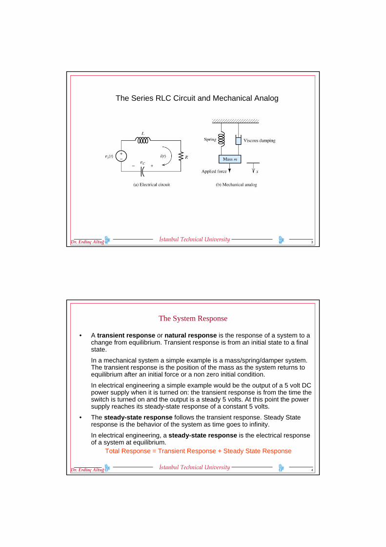
The Purpose of the Experiment:
The responses of a 2nd order system (a RLC circuit) to various inputs will be analyzed and compared with the theoretical results. System response is used to compare performance of various control systems.
In this experiment, a RLC circuit (resistance, inductance and capacitance elements in series) is used as a second order system.
3İstanbul Technical UniversityDr. Erdinç Altuğ
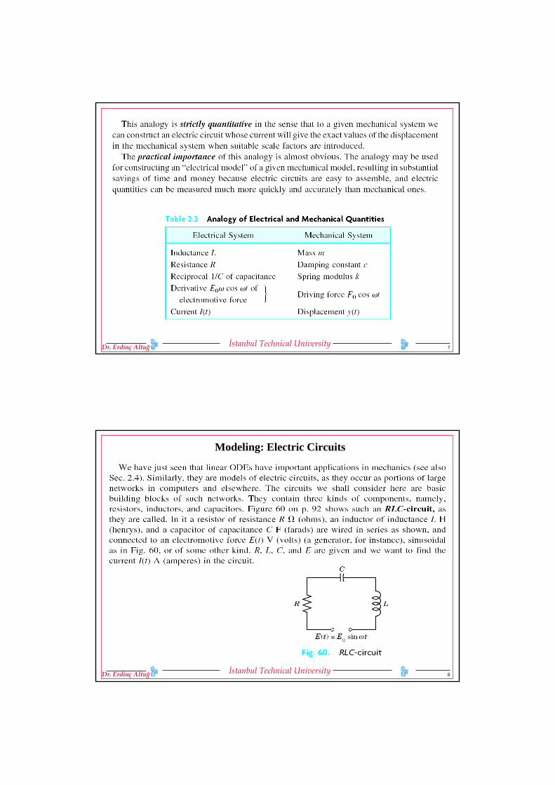
The Series RLC Circuit and Mechanical Analog
4İstanbul Technical UniversityDr. Erdinç Altuğ
• A transient response or natural response is the response of a system to a change from equilibrium. Transient response is from an initial state to a final state.
In a mechanical system a simple example is a mass/spring/damper system. The transient response is the position of the mass as the system returns to equilibrium after an initial force or a non zero initial condition.
In electrical engineering a simple example would be the output of a 5 volt DCpower supply when it is turned on: the transient response is from the time the switch is turned on and the output is a steady 5 volts. At this point the power supply reaches its steady-state response of a constant 5 volts.
• The steady-state response follows the transient response. Steady State response is the behavior of the system as time goes to infinity.
In electrical engineering, a steady-state response is the electrical response of a system at equilibrium.
Total Response = Transient Response + Steady State Response
The System Response

5İstanbul Technical UniversityDr. Erdinç Altuğ
System Response in our experiment
• For Transient Response Analysis, a step input and for Steady State Response Analysis, a sinusoidal input will be applied to the RLC circuit.
• If mathematical system model known => System response can be obtained using Transfer Functions by applying Laplace Transformation
• If no model exists => input is applied and system response analyzed experimentally
You will do the both. (Why?)
6İstanbul Technical UniversityDr. Erdinç Altuğ
Page 96a
Continued
7İstanbul Technical UniversityDr. Erdinç Altuğ
8İstanbul Technical UniversityDr. Erdinç Altuğ
Pages 91-92 Modeling: Electric Circuits

9İstanbul Technical UniversityDr. Erdinç Altuğ
Page 92 (1)
10İstanbul Technical UniversityDr. Erdinç Altuğ
Pages 92-93a
Continued

11İstanbul Technical UniversityDr. Erdinç Altuğ
Pages 92-93b
I: current
Q: charge
12İstanbul Technical UniversityDr. Erdinç Altuğ
Page 93
Solving the ODE (1) for the Current Discussion of Solutions
13İstanbul Technical UniversityDr. Erdinç Altuğ
Page 94
14İstanbul Technical UniversityDr. Erdinç Altuğ
Page 94

15İstanbul Technical UniversityDr. Erdinç Altuğ
Pages 94-95
16İstanbul Technical UniversityDr. Erdinç Altuğ
n
….(1)
Natural frequency
17İstanbul Technical UniversityDr. Erdinç Altuğ
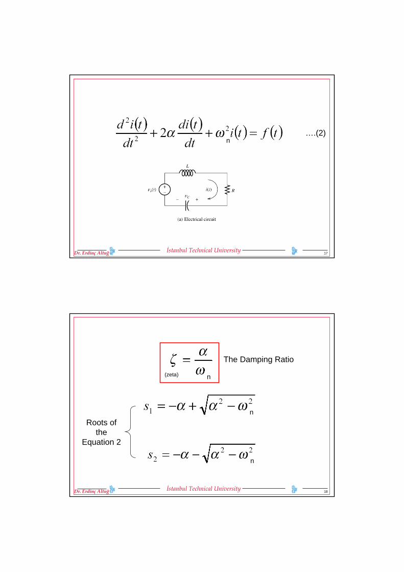
n….(2)
18İstanbul Technical UniversityDr. Erdinç Altuğ
n
n
The Damping Ratio
n
Roots of the
Equation 2
(zeta)

19İstanbul Technical UniversityDr. Erdinç Altuğ
Solution Analysis
n
20İstanbul Technical UniversityDr. Erdinç Altuğ
n

21İstanbul Technical UniversityDr. Erdinç Altuğ
nd
n
1 2( ) cos( ) sin( )t tc n nx t K e t K e tα αω ω− −= +Solution in the form:
22İstanbul Technical UniversityDr. Erdinç Altuğ
Summary: Equations for RLC Circuit (Also in lab sheet)
2
2 2( )2
n
n n
G ss s
ωζω ω
=+ +
2 1n LC
ω =
2R C
Lζ =
2
11LCs RCs+ +
Transfer Function:
( )E s ( )C s
The natural frequency
The damping Ratio
23İstanbul Technical UniversityDr. Erdinç Altuğ
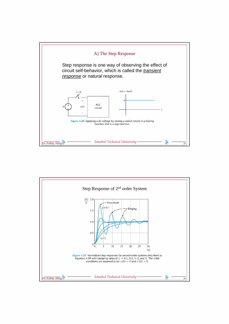
A) The Step Response
Step response is one way of observing the effect of circuit self-behavior, which is called the transient response or natural response.
24İstanbul Technical UniversityDr. Erdinç Altuğ
Step Response of 2nd order System
25İstanbul Technical UniversityDr. Erdinç Altuğ
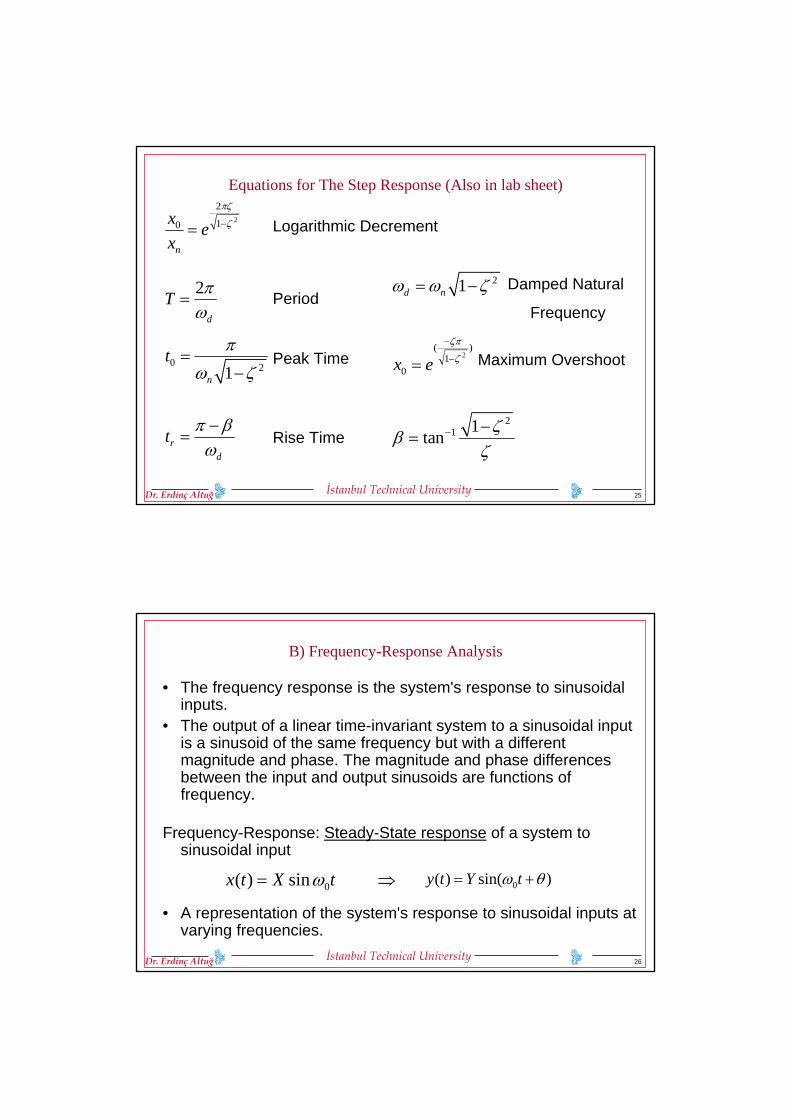
Equations for The Step Response (Also in lab sheet)
2
2
10
n
x ex
πζ
ζ−=
2
d
T πω
=21d nω ω ζ= −
0 21n
t π
ω ζ=
−2
( )1
0x eζπ
ζ
−
−=
rd
t π βω−
=2
1 1tan
ζβ
ζ− −
=
Logarithmic Decrement
Period
Peak Time
Rise Time
Maximum Overshoot
Damped Natural
Frequency
26İstanbul Technical UniversityDr. Erdinç Altuğ
B) Frequency-Response Analysis
• The frequency response is the system's response to sinusoidal inputs.
• The output of a linear time-invariant system to a sinusoidal input is a sinusoid of the same frequency but with a different magnitude and phase. The magnitude and phase differences between the input and output sinusoids are functions of frequency.
Frequency-Response: Steady-State response of a system to sinusoidal input
• A representation of the system's response to sinusoidal inputs at varying frequencies.
0( ) sinx t X tω= ⇒ 0( ) sin( )y t Y tω θ= +
27İstanbul Technical UniversityDr. Erdinç Altuğ
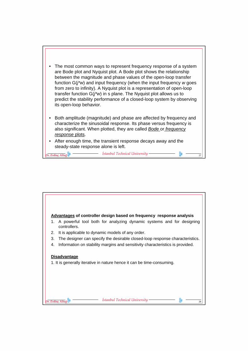
• The most common ways to represent frequency response of a systemare Bode plot and Nyquist plot. A Bode plot shows the relationship between the magnitude and phase values of the open-loop transfer function G(j*w) and input frequency (when the input frequency w goes from zero to infinity). A Nyquist plot is a representation of open-loop transfer function G(j*w) in s plane. The Nyquist plot allows us to predict the stability performance of a closed-loop system by observing its open-loop behavior.
• Both amplitude (magnitude) and phase are affected by frequency and characterize the sinusoidal response. Its phase versus frequency is also significant. When plotted, they are called Bode or frequency response plots.
• After enough time, the transient response decays away and the steady-state response alone is left.
28İstanbul Technical UniversityDr. Erdinç Altuğ
Advantages of controller design based on frequency response analysis1. A powerful tool both for analyzing dynamic systems and for designing
controllers.2. It is applicable to dynamic models of any order.3. The designer can specify the desirable closed-loop response characteristics.4. Information on stability margins and sensitivity characteristics is provided.
Disadvantage1. It is generally iterative in nature hence it can be time-consuming.
29İstanbul Technical UniversityDr. Erdinç Altuğ
• After enough time, the transient response decays away and the steady-state response alone is left.
It can be understood in terms of |G(jw)| - magnitude of the Fourier transform of the impulse response (transfer function)∠G(jw) – phase of the Fourier transform of the impulse response (transfer function)
Bode plots are plots of log magnitude and phase against log frequency.
Used to plot a greater range of frequenciesUsed to plot decibel-type informationTransfer function is now “additive”
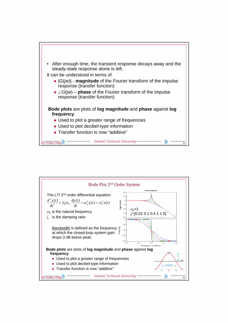
30İstanbul Technical UniversityDr. Erdinç Altuğ
Bode Plot 2nd Order System
The LTI 2nd order differential equation
ωn is the natural frequencyζ is the damping ratio
Bandwidth is defined as the frequency at which the closed-loop system gain drops 3 dB below peak.
)()()(2)( 222
2
txtydt
tdydt
tydnnn ωωζω =++
ωn=1ζ=[0.01 0.1 0.4 1 1.5]
Bode plots are plots of log magnitude and phase against log frequency.
Used to plot a greater range of frequenciesUsed to plot decibel-type informationTransfer function is now “additive”
31İstanbul Technical UniversityDr. Erdinç Altuğ
Equations for Frequency Response (Also in lab sheet)
21 2p nω ω ζ= −
2
1( )2 1
pG ωζ ζ
=−
1( )2nG ωζ
=
( ) out
in
VGV
ω =
(sec) 360(sec)T
φφ =
0 0.707ζ≤ ≤For the range:
Phase Shift
Resonant Frequency
Magnitude of Resonant Peak
Amplitude Ratio
32İstanbul Technical UniversityDr. Erdinç Altuğ
Modeling in MATLAB% Simulate a series RLC circuit.
% The output is the voltage across the capacitor. % Set the R, L, and C values. R = 2; L = e-2; C = 100E-4;
% Set the system matrices. % xdot = Ax + Bu, y = Cx + Du. A = [0 1/C; -1/L -R/L]; B = [0; 1/L]; C = [1 0]; D = [0];
% Create a Matlab state-space model. sys = ss(A, B, C, D);
% Compute and plot the step response.
[y, t] = step(sys);
plot(t, y);
title('Step Response');
% Compute and plot the zero-state response to a sinusoidal input.
dt = 0.003;
tf = 5;
t = 0 : dt : tf;
u = sin(t);
[ysine, t] = lsim(sys, u, t);
plot(t, ysine);
title('Sine Response');
%To plot the bode diagram
Bode(sys);

33İstanbul Technical UniversityDr. Erdinç Altuğ
Lab Procedure
1. Set-up the circuit (Oscilloscope, Signal Generator, Resistance, Inductance, Capacitance, Connection Cables)
2. Apply Step input to the RLC circuit3. Change R, L, and C values and observe effect of each element on the
system (oscillations, steady-state error, etc.) Pick a good response.4. Calculate theoretical values for and . Determine the
experimental values.5. Switch input to Sin wave. (Frequency Response Analysis)6. Increase the value of the Sine input, and read the output and phase
difference. Fill the table.7. Calculate the amplitude ratio, phase difference. Plot Bode diagrams using
Table.8. Plot Bode diagrams using R, L, and C values. (Theoretical) 9. Compare the theoretical and the experimental results, explain the reasons
for the differences.
nω ζ