High-Speed Rail IDEA Program

Magnetometer Sensor Feasibility for Railroad and Highway Equipment Detection Final Report for High-Speed Rail IDEA Project 53 Prepared by: Jeff Brawner K. Tysen Mueller SENSIS Corporation, Seagull Technology Center June 2006

INNOVATIONS DESERVING EXPLORATORY ANALYSIS (IDEA) PROGRAMS MANAGED BY THE TRANSPORTATION RESEARCH BOARD This investigation was performed as part of the High-Speed Rail IDEA program supports innovative methods and technology in support of the Federal Railroad Administration’s (FRA) next-generation high-speed rail technology development program. The High-Speed Rail IDEA program is one of four IDEA programs managed by TRB. The other IDEA programs are listed below. • NCHRP Highway IDEA focuses on advances in the design, construction, safety, and

maintenance of highway systems, is part of the National Cooperative Highway Research Program.

• Transit IDEA focuses on development and testing of innovative concepts and methods for improving transit practice. The Transit IDEA Program is part of the Transit Cooperative Research Program, a cooperative effort of the Federal Transit Administration (FTA), the Transportation Research Board (TRB) and the Transit Development Corporation, a nonprofit educational and research organization of the American Public Transportation Association. The program is funded by the FTA and is managed by TRB.

• Safety IDEA focuses on innovative approaches to improving motor carrier, railroad, and highway safety. The program is supported by the Federal Motor Carrier Safety Administration and the FRA.

Management of the four IDEA programs is integrated to promote the development and testing of nontraditional and innovative concepts, methods, and technologies for surface transportation. For information on the IDEA programs, contact the IDEA programs office by telephone (202-334-3310); by fax (202-334-3471); or on the Internet at http://www.trb.org/idea IDEA Programs Transportation Research Board 500 Fifth Street, NW Washington, DC 20001

The project that is the subject of this contractor-authored report was a part of the Innovations Deserving Exploratory Analysis (IDEA) Programs, which are managed by the Transportation Research Board (TRB) with the approval of the Governing Board of the National Research Council. The members of the oversight committee that monitored the project and reviewed the report were chosen for their special competencies and with regard for appropriate balance. The views expressed in this report are those of the contractor who conducted the investigation documented in this report and do not necessarily reflect those of the Transportation Research Board, the National Research Council, or the sponsors of the IDEA Programs. This document has not been edited by TRB. The Transportation Research Board of the National Academies, the National Research Council, and the organizations that sponsor the IDEA Programs do not endorse products or manufacturers. Trade or manufacturers' names appear herein solely because they are considered essential to the object of the investigation.

Magnetometer Sensor Feasibility for Railroad and Highway Equipment Detection

HSR IDEA Program Final Report

For the period August/2005 through June/2006

Contract: HSR-53

Prepared for the IDEA Program

Transportation Research Board

National Research Council

Jeff Brawner

K. Tysen Mueller

SENSIS Corporation, Seagull Technology Center

24 June 2006

Acknowledgements

The authors wish to thank the Review Panel for their feedback during the Stage 1 and the Final Briefing of this study. The Review Panel includes:

Chuck Taylor: Transportation Research Board (TRB),

Pete Mills: Federal Highway Administration (FHWA),

Richard Reiff: Transportation Technology Center, Inc., American Association of Railroads (TTCI/AAR),

James Smailes: Federal Railroad Administration (FRA),

Corey Wills: Burlington Northern Santa Fe (BNSF) Railway.

In addition, the authors wish to express a special thanks to Corey Wills along with the BNSF Railway for their support of the field tests that were conducted near Emporia, KS, and in Topeka, KS, April 2006. Finally, the authors wish to thank the TRB HSR IDEA Program for funding this research and to Chuck Taylor for his direction.

Abstract This study investigated the feasibility of using Anisotropic Magneto-Resistive (AMR) magnetometers to detect train

or vehicle presence and to determine train speed for the activation of grade crossing warning systems. Laboratory, parking lot, and railroad field tests were performed using 3-axis digital AMR magnetometers for train and vehicle detection as well as speed measurement.

It was determined that the sensors drift with changes in the ambient temperature. However, by periodic bias removals (auto-calibrations), the impact of these bias drifts can be eliminated. It was also determined that the detection distance for vehicles depends on the amount of magnetic material (iron, nickel, or cobalt) and varies as the inverse cubed (3rd) power of the distance from the sensor. Changes in the ambient electro-magnetic field, such as caused by variable current power lines, are also detected with an inverse (1st power) distance relationship. Hence, electromagnetic interference may travel a longer distance than a magnetic signature, depending on the magnitudes of these two signals.

Overall, it was found that the 3-axis measurement capability of the AMR magnetometers permits the unique identification of different vehicles. It also permits the separation of vehicle signatures from noise signatures. Hence, these magnetometers provide an alternative, more flexible, approach for activating crossing warning systems than the current use of track circuits.

Keywords 1. Magnetometers

2. Anisotropic Magneto-Resistive (AMR) magnetometers

3. Grade crossings

4. Grade crossing warning system activation

5. Train detection sensors

6. Train speed determination sensors

7. Vehicle detection sensors

8. Vehicle magnetic signatures

TABLE OF CONTENTS 1 Executive Summary .......................................................................................................................1

1.1 Motivation ..............................................................................................................................1 1.2 AMR Magnetometer Concept ................................................................................................1 1.3 Principal Findings ..................................................................................................................2

2 IDEA Product.................................................................................................................................3 3 Concept and Innovation .................................................................................................................3 4 Investigation ...................................................................................................................................5

4.1 Sensor Characterization..........................................................................................................5 4.1.1 Temperature Dependence...............................................................................................5 4.1.2 Orientation – Dependence..............................................................................................6 4.1.3 Compass Direction Dependence ....................................................................................6 4.1.4 Electromagnetic Field Sensitivity ..................................................................................7 4.1.5 Four-Quadrant Location Determination Capability .......................................................7

4.2 Sensor Characterization Lab Tests.........................................................................................8 4.2.1 Data Collection Method .................................................................................................8 4.2.2 Single Vehicle Signatures ..............................................................................................8 4.2.3 Multiple Vehicle Signatures.........................................................................................11

4.3 Field Tests ............................................................................................................................12 4.3.1 Test Plan.......................................................................................................................12

4.4 Field Test results ..................................................................................................................13 4.4.1 Overview ......................................................................................................................13 4.4.2 Sensor Characterization Tests ......................................................................................15 4.4.3 Signature Identification................................................................................................17 4.4.4 Locomotive Speed Test................................................................................................17 4.4.5 Crossing Tests ..............................................................................................................20

4.5 Plans for Implementation .....................................................................................................22 5 Review Panel input.......................................................................................................................24

5.1 Stage 1 Review Panel Feedback...........................................................................................24 5.2 Stage 4 Final Briefing Feedback ..........................................................................................24

6 Summary and Conclusions...........................................................................................................25 6.1 Goals demonstrated ..............................................................................................................25

6.1.1 Vehicle Detection and Identification: ..........................................................................25 6.1.2 Locomotive Noise Interference Signature: ..................................................................25 6.1.3 Four-Quadrant Train Location: ....................................................................................25 6.1.4 Detection of Rail Cars Left in Crossing:......................................................................25 6.1.5 Signature Repeatability: ...............................................................................................25

6.2 Sensor Limitations................................................................................................................26 6.2.1 AMR Sensor Selection.................................................................................................26 6.2.2 Analog AMR Sensors ..................................................................................................26 6.2.3 Digital AMR Sensors ...................................................................................................26

6.3 Conclusions ..........................................................................................................................26 7 References ....................................................................................................................................27

1

1 EXECUTIVE SUMMARY

1.1 MOTIVATION

In the United States, one person a day dies at a railroad crossing, based on statistics compiled in 2004. Each fatality is estimated to cost the industry $2.7M-$3M. Of the 150K public crossings in the US, only approximately 50% have active warning systems such as gates, flashing lights, bells, or combinations thereof. Hence the need for cost-effective, reliable active crossing warning systems is apparent.

Currently, warning system activation uses track circuits to determine the presence of approaching trains. When a locomotive’s or railcar’s wheels and axles shunt an electrical current away from the signal relay, the relay drops out and activates the warning signal. Track circuits, however, are regarded as costly and requiring high maintenance. They are also susceptible to “loss of shunt” when highly resistive, thin films on wheels and rail can affect their performance. This loss of shunt can allow the premature opening of the crossing-gate even though a train is still in the crossing island.

Another problem with today's active warning systems is that a motorist can become trapped in the island of a four quadrant gate system. This may occur since the track circuits cannot determine the presence of a car at the crossing. If a motorist moves too slowly to make it out of the island before the exit gate closes, this can impede the vehicle’s clearing the crossing.

Applications of this magnetometer senor technology to be investigated also include detection of Hi-Rail and other track inspection and maintenance equipment on or near the track and detection of detection of right-of-way incursions by non-railroad vehicles and equipment.

1.2 AMR MAGNETOMETER CONCEPT

An alternative crossing sensor system is proposed that involves the use of Anisotropic Magneto-Resistive (AMR) magnetometers. The system architecture for this Magnetometer Activated Gate System (MAGS) concept is shown in Figure 1.

This figure shows that multiple AMR sensors are used to detect the presence and speed of an approaching train as well as monitor the crossing island for trapped vehicles and the end of the train. The distributed MAGS sensors are connected via wireless communication links with a MAGS central processing unit (CPU). This CPU takes the raw sensor measurements and filters and calibrates these measurements. In addition, it applies various signal processing algorithms that will determine the speed, direction, location, and signature of the train and vehicles.

AMR magnetometers are currently available in analog or digital form as shown in Figure 2. In addition, they can be obtained in 1-, 2-, or 3-axis configurations.

AMR magnetometers sense the change in the earth’s ambient magnetic field that is caused by a

metallic object. In the absence of any other metal objects, a vehicle will disturb the earth’s magnetic field as illustrated in Figure 3. In Figure 3, the vertical lines represent the horizontal components of the earth’s magnetic field that are locally nearly parallel. The presence of a large metal object causes these magnetic lines to be distorted. The AMR magnetometer measures this change in the earth’s magnetic field. Hence, when a car drives past the middle magnetic sensor in the forward direction, the magnetometer measures the change in the magnetic field, as shown in the curve in the lower left-hand corner. When the car reverses its direction, the mirror image curve in the lower right-hand corner is obtained.

AMR magnetometers are superior to previous magnetometers that have been evaluated for crossing system activation. The AMR sensors not only detect train presence by detecting the disturbances in the Earth’s magnetic field, as do other magnetometers, but also display the unique magnetic signature of a metal object moving past the sensor. This

FIGURE 1 Magnetometer-Activated Gate System (MAGS)

Architecture

2

signature changes in relationship to the: type of object (vehicle presence), location from the sensor (track location), direction of movement (vehicle moving forward or reverse), and speed (using two sensors).

Constant environmental disturbances, such as electro-magnetic interference or metal contaminants along the track, are eliminated via auto-calibration. With auto-calibration, the recent ambient readings are combined into a bias estimate that is removed from future readings. With this magnetic signature measurement capability, the AMR magnetometer can eliminate false alarms by identifying the differences between a train, maintenance vehicle and other magnetic sources. Furthermore, unlike other magnetometers, the AMR magnetometer has rapid signal dissipation after an object departs. This will allow for a quick grade-crossing warning recovery.

1.3 PRINCIPAL FINDINGS

Most of the work involved the testing and evaluation of the digital AMR magnetometers. Both the analog and digital AMR sensors were tested in the lab. The digital sensors were tested using highway vehicles in a parking lot, in surrounding streets, and at a railroad crossing. The railroad crossing tests were performed in cooperation with the BNSF Railway on the dual mainline tracks east of Emporia, KS, and at the locomotive maintenance facility in Topeka, KS.

It was discovered during the Stage 1 sensor review that Honeywell is the only one manufacturer of complete AMR sensors. According to their sensor expert, there are companies in Europe that make the sensing element, but don’t provide the supporting electronic circuitry for a completed sensor. The Honeywell sensors can be purchased as sensing elements (analog sensors) or as completed sensors (digital sensors). They sell their digital sensors as 1, 2, or 3 axis (X, Y, Z axis) detectors.

Trains were shown to have their own unique magnetic signatures. These signatures are very large in magnitude, relative to cars, and are very complex due to the number of cars and the amount of ferrous material. It should be possible to use some part of these signatures as a tripwire for activating crossing warning devices.

Locomotive Electromagnetic Interference (EMI) was detected. However, it didn’t appear to be very large and shouldn’t create problems with detecting trains using AMR magnetometers.

A single AMR magnetometer has the ability to detect in which of four quadrants a metallic object has moved by examining the X-Y (local horizontal) axes signatures, so-called four-quadrant location detection. Four-quadrant location detection of trains could not be made at this time due to insufficient field data. Tests with a car in the parking lot showed what appears to be a different X-Y signature depending on the movement of the car between quadrants.

Detection of rail and street vehicles, both approaching the crossing and sitting in the crossing island, was achieved. Likewise rail vehicles also produced their own signatures that showed when they were either entering or sitting in the island. The rail vehicle signatures are so large that they cannot be mistaken for street vehicles.

Signature repeatability was established with cars in the parking lot by repeatedly driving back and forth over a sensor. However, signature repeatability could not be established in the field for trains since a train could not pass the sensor multiple times to confirm its signature.

Analog Mag [1] Digital Mag [2]

FIGURE 3 Directional Signature of Car [3]FIGURE 2 Analog and Digital Sensors

3

The best sensor location was determined to be 7.5ft offset from the first (nearest) rail. This distance reduced signal saturation and vibration caused by passing trains. This distance was also used as the minimum approach threshold for street vehicles approaching the crossing and, when crossed, they were considered to be in the crossing.

2 IDEA PRODUCT The MAGS concept involves a distributed sensor network as shown in Figures 1 and 4.

In Figure 4, Sensors 1 and 2 (S1 and S2) are used to determine the initial presence and speed of an approaching train. They are placed at a distance from the highway crossing, such that when the train passes at the maximum speed limit and the crossing gates are activated, there is a 20-30 sec delay before the train reaches the crossing. Any production version of this system would also include the capability to provide for a constant warning time, regardless of train speeds.

Since a train may slow down or even stop before reaching the crossing, Sensor 3 (S3) verifies that the initial speed has not changed. If it has changed, and there is a significant delay before the train is expected to reach the crossing, the gates can be opened again and lowered at a later time.

Finally, Sensors 4 and 5 (S4 and S5) monitor the crossing island for trapped motor vehicles. These sensors also determine when the last rail car of a train has passed and it is safe for the gates to be reopened. While the crossing gate and its activation hardware are not part of the MAGS system, the MAGS system provides the information necessary for proper warning system operation.

Other applications could employ installing sensors in the middle of the road along both directions in order to record each vehicle’s unique signature as it passes over the sensors. This information could be used to help distinguish one vehicle from another, bus vs. large truck, or determine the speed of an approaching vehicle. This sensor technology could also be used to detect Hi-Railers and other track maintenance equipment on or adjacent to the track. In addition, it could be used for the detection of right-of-way or restricted area incursions by non-railroad vehicles and equipment.

3 CONCEPT AND INNOVATION AMR magnetometers sense the change in the ambient magnetic field that is caused by a metallic object. A metallic object is any object that contains iron, nickel, or cobalt. They can only detect a metallic object relative to an ambient baseline. Hence, if car is stopped at the time of an auto-calibration (nulling the current ambient reading) and does not move, the car cannot be detected.

In the absence of any other metal objects, a vehicle will disturb the earth’s magnetic field, as was illustrated in Figure 3. In Figure 3, the vertical lines represent the horizontal components of the earth’s magnetic field that are locally nearly parallel. The presence of a car causes these magnetic lines to be distorted. The AMR magnetometer measures this change in the earth’s magnetic field. Hence, when a car drives past the middle magnetic sensor in the forward direction, the magnetometer measures the change in the magnetic field, as shown in the curve in the lower left-hand corner. When the car reverses, the mirror image curve in the lower right-hand corner is obtained.

Several non-AMR magnetometers were tested at the Transportation Technology Center, Inc. (TTCI), Pueblo, CO, in 1999 [4]. A series of tests were performed on different rail and street vehicle detection devices to assess their potential

TRAIN

SENSORS:

CAR 1

CAR 2

S1 S2 S3 S4

S5

FIGURE 4 MAGS Distributed Sensor Architecture for Crossing Gate Activation

4

for activation of crossing warning systems. One test utilized dual magnetic anomaly detectors having two sense coils mounted at right angles to each other. This was combined with vibration detectors to compensate for sensors that became saturated by nearby magnetic objects. The tests simulated detection of trains and street vehicles entering the island along with early warning of train arrival. A 20-second warning for train arrival and a 2-second maximum release time after the train cleared the crossing was considered a successful test. From these tests a pass/fail list was created for each type of detection system.

Problems with these magnetic anomaly systems included their inability to release the gate if a rail vehicle reversed its direction (no directionality detection) or a hi-rail vehicle left the track and didn’t pass the second detector. Another problem was a magnetic “ghost” image (sensor delay) that detected train presence in the island long after train departure. In both cases a manual reset was needed to release the gate.

The AMR magnetometers were shown to be superior to the previously-tested magnetometers for crossing activation. The AMR sensors not only detect train presence by detecting the disturbances in the Earth’s magnetic field, as other magnetometers do, but also display the unique magnetic signature of a metal object moving past the sensor. This signature changes in relationship to the: type of object (vehicle presence), location from the sensor (track location), direction of movement (vehicle moving forward or reverse), and speed (using two sensors).

Environmental disturbances, such as electromagnetic interference or metal contaminants along the track, are eliminated via auto-calibration. With this magnetic signature measurement capability, the AMR magnetometer can eliminate false alarms by identifying the differences between a train, maintenance vehicle and other metallic sources. Furthermore, unlike other magnetometers, the AMR magnetometer has rapid signal dissipation after an object departs. This will allow for a quick grade-crossing warning recovery.

The three orthogonal AMR signatures are unique. Hence, a vehicle detection system could use the lateral axis for precise determination of the point of closest approach. It could use the two horizontal axes for quadrant location detection. Finally, it could use the combined signal magnitude for initial/final vehicle detection.

AMR magnetometers are currently available in analog or digital form as was shown in Figure 2. In addition, they can be obtained in 1-, 2-, or 3-axis configurations.

5

4 INVESTIGATION The investigation involved tests of the analog and digital AMR sensors in the laboratory. In addition, the digital sensors were tested in the parking lot and surrounding streets as well as near railroad tracks during field tests performed with the help of the BNSF Railway.

4.1 SENSOR CHARACTERIZATION

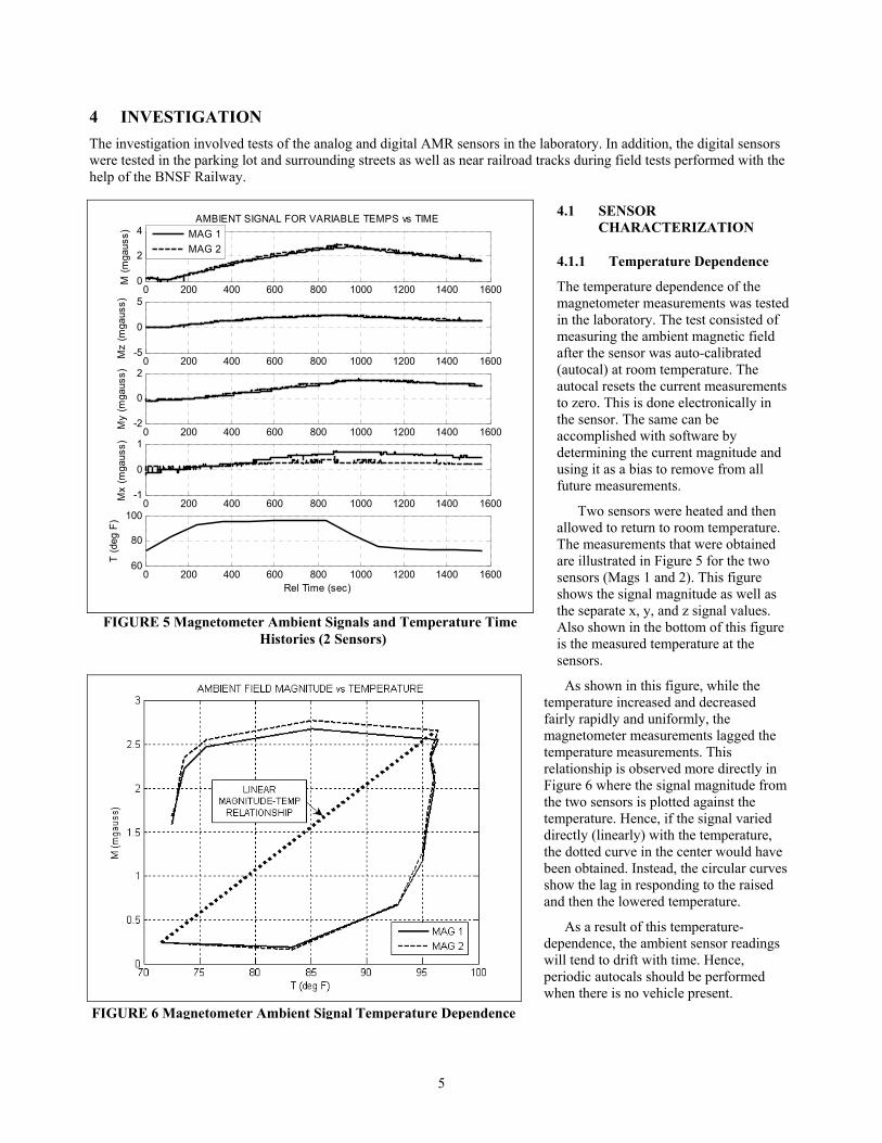
4.1.1 Temperature Dependence

The temperature dependence of the magnetometer measurements was tested in the laboratory. The test consisted of measuring the ambient magnetic field after the sensor was auto-calibrated (autocal) at room temperature. The autocal resets the current measurements to zero. This is done electronically in the sensor. The same can be accomplished with software by determining the current magnitude and using it as a bias to remove from all future measurements.

Two sensors were heated and then allowed to return to room temperature. The measurements that were obtained are illustrated in Figure 5 for the two sensors (Mags 1 and 2). This figure shows the signal magnitude as well as the separate x, y, and z signal values. Also shown in the bottom of this figure is the measured temperature at the sensors.

As shown in this figure, while the temperature increased and decreased fairly rapidly and uniformly, the magnetometer measurements lagged the temperature measurements. This relationship is observed more directly in Figure 6 where the signal magnitude from the two sensors is plotted against the temperature. Hence, if the signal varied directly (linearly) with the temperature, the dotted curve in the center would have been obtained. Instead, the circular curves show the lag in responding to the raised and then the lowered temperature.

As a result of this temperature-dependence, the ambient sensor readings will tend to drift with time. Hence, periodic autocals should be performed when there is no vehicle present.

0 200 400 600 800 1000 1200 1400 16000

2

4AMBIENT SIGNAL FOR VARIABLE TEMPS vs TIME

M (m

gaus

s)

MAG 1MAG 2

0 200 400 600 800 1000 1200 1400 1600-5

0

5

Mz

(mga

uss)

0 200 400 600 800 1000 1200 1400 1600-2

0

2

My

(mga

uss)

0 200 400 600 800 1000 1200 1400 1600-1

0

1

Mx

(mga

uss)

0 200 400 600 800 1000 1200 1400 160060

80

100

T (d

eg F

)

Rel Time (sec)

FIGURE 5 Magnetometer Ambient Signals and Temperature Time

Histories (2 Sensors)

FIGURE 6 Magnetometer Ambient Signal Temperature Dependence

6

4.1.2 Orientation – Dependence

Once the sensors are placed into position and a cal has been preformed, the sensors cannot be moved. Any movement can cause changes in the ambient readings. If movement occurs via natural changes or settling of the earth, a new cal can be preformed in order to reset or create a new ambient condition.

Sensors placed 7.5ft and 15ft from the first rail didn’t appear to suffer from any vibration caused by a passing train during the field tests performed with the BNSF Railway near Emporia, KS. Ground vibrations would not produce a signature that resembles a passing vehicle.

4.1.3 Compass Direction Dependence

Toward the end of the lab and parking let tests, a simple test was conducted to determine whether the test results depend on the direction of motion relative to the earth’s magnetic field. Most of the lab and parking lot tests had been performed in a nearly north-south direction, since the lab bench and parking lot used for the tests were oriented in that direction.

The lab test consisted of performing the same experiment at different compass directions by varying the direction incrementally by 45 deg from north. The test consisted of aligning the magnetometer x-axis along the selected compass direction and moving a small metal object (stapler) back and forth along that direction. The resultant signal magnitudes are illustrated in Figure 7.

In Figure 7, the first measurement in the upper left-hand figure is taken along the north direction. Then moving in a clock-wise direction incremented at 45 deg, the remaining measurements were taken with the south direction, found in the lower right-hand side of Figure 7.

What is surprising is that compass directions that are opposite of each other (north and south), don’t have the same magnitude. Furthermore, the measurement magnitudes uniformly decrease from north and northeast to the measurements in the south and southwest.

The most likely explanation is that the stapler was partially magnetized. Hence, when aligned in certain directions with respect to the earth’s magnetic field, stapler magnetism could effectively minimize the effects from the earth’s magnetic field.

0 20 40 60 800

10

20

N (m

gaus

s)

0 20 40 600

10

20

NE

(mga

uss)

0 20 40 600

10

20

NW

(mga

uss)

0 20 40 600

10

20

E (m

gaus

s)

20 40 600

10

20

W (m

gaus

s)

0 20 40 600

10

20

SE

(mga

uss)

0 10 20 30 40 500

10

20

SW

(mga

uss)

Relative Time (sec)0 20 40 60

0

10

20

S (m

gaus

s)

Relative Time (sec)

MAGNITUDE vs COMPASS DIRECTIONS

FIGURE 7 Signature Magnitude of Small Metal Object (Stapler) vs. Compass Direction (Both sensor and measurements are aligned

with compass directions)

FIGURE 8 Compass Tests with Fiero (N vs. S)

0 5 10 15 20 25 30 35 4010

0

101

102

Compass TEST FWD BWD North & South 2 (LPF) SIG MAGNITUDES vs TIME

M (m

gaus

s) N

orth

0 5 10 15 20 25 30 35 4010

0

101

102

M (m

gaus

s) S

outh

Relative Time (sec)

7

This phenomenon has not been observed with larger metallic objects such as vehicles. Figure 8 shows North vs. South test performed with a Fiero sports car in a parking lot. The vehicle slowly passed the sensor several times at a distance of about 2 feet with the sensor first facing north and than the test was repeated facing south. As seen in Figure 8, the magnitudes of the two tests are about the same – both curves peak around 40 mgauss. Hence, there is no apparent magnetic affect from a passing vehicle.

4.1.4 Electromagnetic Field Sensitivity

Since an overhead power line has a magnetic field, this field will be added to the earth’s magnetic field. If the current in the power line is fairly uniform, the AMR magnetometer can null out these combined ambient measurements. However, when any vehicle or metal object disturbs this ambient magnetic field, the sensor will measure this change in the ambient magnetic field.

During one of the tests, data was collected for an electric rapid transit train as it left the transit station at some distance from the sensor and then passed the sensor shown in Figure 9. The resultant measurement histories for the x, y, and z signals are shown in Figure 10. The x-axis is parallel to the tracks, the y-axis is perpendicular to the tracks, and the z-axis is up.

As shown in Figure 10, there is a clear distinction between the transit vehicle signature (3rd circled area from left) and the three disturbance signatures. The key difference in the transit vehicle signature is noted in the sinusoidal y signal while the transit vehicle moves along the x-direction.

The first disturbance is believed to occur when the transit vehicle accelerates from the station. This causes a significant change in the power line used by this electric vehicle. The

remaining two disturbances may be associated with some dynamic braking of the transit vehicle. It was noted that the transit vehicle tended to slow down when they saw that these measurements were being taken.

The station was several hundred feet away while the transit vehicle passed at an approximate distance of 60 ft. The reason that the three disturbances occur before or after the transit signal was present is due to the fact that the disturbance signals have inverse distance dependence, while the transit vehicle signal probably has an inverse cubed or higher dependency.

Field test results with a fully powered locomotive established that the electromagnetic field generated near the locomotive is small relative to its magnetic

signature. These results will be discussed under the Field Test discussion.

4.1.5 Four-Quadrant Location Determination Capability

When an object moves past a single sensor from different locations (quadrants) around the sensor, a unique combination of the two horizontal signatures is obtained, as illustrated in Figure 11. This feature permits the determination of the object in any of the four quadrants – so-called four-quadrant detection. In Figure 11, a simple metallic object was moved in front and behind an AMR sensor in the lab. If this capability is demonstrated for more complex metal objects trains, it might be utilized to determine if a train is on a mainline vs. siding track. Also, it might be used to rule out non-logical detections such as a train apparently coming from a location without a track.

FIGURE 9 Electric Rapid Transit Train

-40

-30

-20

-10

0

10

20

30

40

0

6.7

13.4

20.1

26.8

33.5

40.2

46.9

53.6

60.3 67

73.7

80.4

87.1

93.8

100

107

114

Sec

Milli

gaus

s

x y z

Train

FIGURE 10 Transit Vehicle and Noise Signatures

8

4.2 SENSOR CHARACTERIZATION LAB TESTS

4.2.1 Data Collection Method

Data from a digital AMR magnetometer was connected to the Data Acquisition System (DAQ). This DAQ System collected all sensor data and sent commands to the sensors for setup and calibration. As shown in Figure 12 and 13, there are four digital magnetometer sensors and a digital range finder. The range finder was used to determine the distance from a test object such as a locomotive or car. By numerically differentiating the range finder time history, the speed of the test object can also be determined.

Before each test run an autocal is performed. Next, the text document logging location with a date, time and test name are created for each sensor. Then data logging starts and data is collected for the sensor during that test run.

4.2.2 Single Vehicle Signatures

Magnetic field signatures for a number of vehicles were measured. These included the controlled tests using a sports car (Fiero) and an SUV (Lexus). In addition, it included signatures of an SUV and truck on the street. Finally, the signature of an electric rapid transit train with 2 cars on tracks was measured.

FIGURE 12 Data Acquisition System FIGURE 13 Data Acquisition System Diagram

4-Quad Travel path4-Quad Travel path

x y z

x y zX Y Z

FIGURE 11 Four Quadrant Signals with Vehicle Moving Along X-Axis (Shown for simple metallic object)

Mag

+X

+Y

FWDVehicle paths

FWD

-X

-Y

Q1 Q2

Q3 Q4

Mag

+X

+Y

FWDVehicle paths

FWD

X

-Y

Q1 Q2

Q3 Q4

x y z

9

4.2.2.1 Small Car (Fiero) Signatures

The signal was recorded by driving the car twice over the sensor along the x-direction, both forward and reverse. The car is shown in parking lot during a simulated crossing test in the right-hand side of Figure 14.

The corresponding signal magnitude as well as x, y, and z signal time histories are illustrated in Figures 15-18.

Each figure shows the forward signal in the left-hand panels and

the reverse signals in the right-hand panels.

FIGURE 15 Fiero Sensor Drive-Over Magnetic Field Magnitude Time History

FIGURE 16 Fiero Sensor Drive-Over Z-Axis (Vertical) Magnetic Field Time History

FIGURE 17 Fiero Sensor Drive-Over Y-Axis (Lateral) Magnetic Field Time History

FIGURE 18 Fiero Sensor Drive-Over X-Axis (Along Track) Magnetic Field Time History

FIGURE 14 Vehicles used during the simulated train tests, SUV and Fiero

10

Each of the figures shows that the signal is fairly repeatable, with the reverse signature the mirror image of the forward signature for all four signals. It is difficult to associate the 3 peaks with any particular parts of this car in part because the engine is in the rear of this vehicle.

Parking lot tests indicated a detection distance greater than 90 ft. At 90 ft, which corresponded to the maximum distance from the laser range finder, there was already a measurable signal for the car.

4.2.2.2 Large Car (Lexus SUV) Signatures The same experiment was repeated with a larger car, a Lexus SUV, as shown in the left-hand side of Figure 14. Specifically, the SUV was driven over the sensor along the x-direction 3 times, both forward and reverse. The resulting signal histories are presented in Figures 19-22.

0 5 10-400

-200

0

Z FIELD FOR LEXUS SUV FORWARD & REVERSE OVERPASSES

FIE

LD 1

(mga

uss)

0 5 10 15 20-400

-200

0

0 5 10 15 20-400

-200

0

FIE

LD 2

(mga

uss)

0 5 10 15-400

-200

0

0 5 10-400

-200

0

FIE

LD 3

(mga

uss)

RELATIVE TIME FORWARD (sec)0 5 10 15 20

-400

-200

0

RELATIVE TIME REVERSE (sec)

FIGURE 20 SUV Sensor Overpass Magnetic Z Field Time History

0 5 10-400

-200

0

200Y FIELD FOR LEXUS SUV FORWARD & REVERSE OVERPASSES

FIE

LD 1

(mga

uss)

0 5 10 15 20-400

-200

0

200

0 5 10 15 20-400

-200

0

200

FIE

LD 2

(mga

uss)

0 5 10 15-400

-200

0

200

0 5 10-400

-200

0

200

FIE

LD 3

(mga

uss)

RELATIVE TIME FORWARD(sec)0 5 10 15 20

-400

-200

0

200

RELATIVE TIME REVERSE (sec)

FIGURE 21 SUV Sensor Overpass Y Magnetic Field Time History

0 5 10-200

0

200X FIELD FOR LEXUS SUV FORWARD & REVERSE OVERPASSES

FIE

LD 1

(mga

uss)

0 5 10 15 20-200

0

200

0 5 10 15 20-200

0

200

FIE

LD 2

(mga

uss)

0 5 10 15-200

0

200

0 5 10-200

0

200

FIE

LD 3

(mga

uss)

RELATIVE TIME FORWARD (sec)0 5 10 15 20

-200

0

200

RELATIVE TIME REVERSE (sec)

FIGURE 22 SUV Sensor Overpass Magnetic X Field Time History

0 5 100

200

400

FIELD MAGNITUDE FOR LEXUS SUV FORWARD & REVERSE OVERPASSES

FIE

LD 1

(mga

uss)

0 5 10 15 200

200

400

0 5 10 15 200

200

400

FIE

LD 2

(mga

uss)

0 5 10 150

200

400

0 5 100

200

400

FIE

LD 3

(mga

uss)

RELATIVE TIME FORWARD (sec)0 5 10 15 20

0

200

400

RELATIVE TIME REVERSE (sec)

FIGURE 19 SUV Sensor Drive Over Magnetic Field Magnitude Time History

11

As shown in these figures, the forward signatures are fairly consistent, while the reverse signatures are mirror images of the forward signatures. For this vehicle, the engine is in the front and probably represents the larger spike in the magnitude signature.

Comparing the Fiero to the SUV signal magnitude history, it is clear that the two have distinct signatures. For either vehicle, the magnitude history is probably sufficient for vehicle identification.

4.2.3 Multiple Vehicle Signatures

4.2.3.1 Two Cars Passing at Crossing

In this test, the problem of detecting the presence of two cars when both are traveling in the same direction on a 4-lane highway over a single-track railroad crossing is investigated. Specifically a large car (SUV) is properly stopped by the crossing gate in the outside lane closest to the sensor for that lane. On the inside lane a smaller car (Fiero) passes the SUV, enters the crossing island, stops, and then proceeds through the crossing. Next it stops again and finally reverses back through the crossing. Hence for this multi-car scenario, would the four sensors at the four corners of the crossing island be able to identify the small car in the presence of the larger car?

It was discovered during this test that the sensor closest to the SUV was saturated and not much data was seen other then the SUV presence. The other 3 sensors could see both the Fiero and the SUV as they entered next to the rail. In this report only the most relevant data is displayed, which is Figure 23. This is the cross-track sensor placed 7.5ft from the far rail diagonally from both vehicles on the other side of the street labeled Mag 1 for this test. This sensor clearly shows the SUV enter and the Fiero follows a short time later. Further, it detects that the Fiero has moved close to it (large deflections) and sits for some time (plateau) before passing the sensor (large sinusoidal spikes) indicating the car is now moving out of the island.

Based on this test case, it is possible to use a sensor other than the closest sensor to separately monitor the SUV and Fiero. In a more complex and realistic four-lane highway example where a car may be in each of the four lanes near the crossing island, probably all four sensors would be required to monitor all four lanes.

4.2.3.2 Train-Car Crossing Simulation Test

During this parking lot test scenario, the vehicle (Fiero) sits 7.5’ from first rail as a train (SUV) approaches from the left, sits, and then reverses out of island. This test is used to demonstrate multiple

vehicle entry, presence, and exit detection by the four sensors.

The data for one of the four magnetometers (Mag 4) is shown in Figure 24. This sensor is located diagonally opposite both the stopped car and the approaching train.

-60

-40

-20

0

20

40

60

80

100

8090

.310

111

112

113

114

215

216

217

318

319

320

421

422

423

524

525

526

527

628

629

6

Sec

Cou

nts

x y z

SUV enters and sits at gate

Passing Mag 1 FWD

Car sits passed M1

Car Exits in REV

No Vehicles

Non-Test Vehicles Enters

Carenters island

Car waits in islandSU

V Pr

esen

ce

FIGURE 23 Parking Lot Test of Passing Car at Simulated Crossing (Mag 1 Sensor Located Diagonally across Street from 2 Cars; 15 counts/mgauss)

12

The data in Figure 24 shows that an ambient condition exists with no track or street vehicles near the crossing. Next it shows a car approaching and waiting followed by the simulated train. The train approaches, enters, waits, and exits out of the island. The car is seen before the train arrives and after the train departs.

4.3 FIELD TESTS

4.3.1 Test Plan

The field tests, summarized in Table 1 below, focused on the use of AMR magnetometers to detect and identify rail vehicles and highway vehicles at a railroad

crossing. For comparison, some of these tests are tests that were completed in the lab or in the parking lot. Other tests are additional tests that were not originally considered either because they would not be possible without trains or because of improved test equipment.

The field test goals are to demonstrate: 1. Track vehicle detection and identification 2. Locomotive noise interference signature 3. Directional detection (mainline vs. siding track or street vs. track) 4. Detection of train cars left in crossing (Train cars remaining on track) 5. Signature repeatability

-100

-80

-60

-40

-20

0

20

40

60

80

10011

5.40

122.

1512

8.90

135.

6514

2.40

149.

1515

5.90

162.

6516

9.40

176.

1518

2.90

189.

6519

6.40

203.

1520

9.90

216.

6522

3.40

230.

1523

6.90

243.

6525

0.40

257.

1526

3.90

Sec

Cou

nts

x y z

Car (Fiero) Enters

Train (SUV)

FIGURE 24 Parking Lot Simulation of Train Passing Through Crossing with Waiting Car

(Mag 4 sensor diagonally across from car, other side of crossing; 15 counts/mgauss)

13

TABLE 1 Proposed Field Test Matrix

TEST TEST NAME OBJECTIVE SENSORS

Sensor Characterization

Test 1 Sensor Placement Determine the best lateral placement of sensors from rail to maximize detection and avoid signal saturation. 4

Test 2 Locomotive Noise Identify & record locomotive Electro-Magnetic Interference (EMI) noise signature 2

Test 3 Detection Distance Determine the maximum detectable distance of an approaching train 2

Vehicle Signature Identification

Test 4 Pass-By Record different passing rail vehicle signatures 2

Test 5 Locomotive Speed Determine & verify speed of passing train using 2 sensors linked by radio modems plus a third sensor connected by cable 3

*Test 6 Gate Activation Time Determine if system can give 30-second warning before train arrives at gate. 3

*Test 7 4-Quad Detection Determine direction and identify track of two trains passing on different tracks with a single sensor 1

Crossing Tests (Rail-Highway Vehicle Interactions)

Test 8 Gate Cross Traffic Verify highway vehicle correct stopping distance at gate. Verify highway-rail vehicle detection at crossing island 4

*Optional Test: Data not needed at this time, recorded by other tests, or can be deduced from other test data.

4.4 FIELD TEST RESULTS

4.4.1 Overview

The mainline tests were performed with the support of Corey Wills, Burlington Northern and Santa Fe (BNSF) Railway. The tests took place east of the Emporia, KS, BNSF yard on 20 April. There were two parallel mainline tracks with an adjoining rural crossing. The tests are summarized in Table 2.

In particular, Tests 8A-8D involves three trains. First, an east-bound freight approaches on the near track and stops short of the MAGS data collection setup (Test 8A). Next, two west-bound freights pass on the far track (Tests 8B and 8C). Finally, the eastbound train continues past the MAGS sensors (Test 8D).

Separate tests were performed on 21 April at the BNSF locomotive maintenance facility in Topeka, KS. These tests consisted of an electromagnetic interference (EMI) test for a stationary locomotive, as summarized in Table 3. Separately, the magnetic signature of a compact hybrid car (Honda Insight), with an aluminum body and engine, were recorded

14

TABLE 2 Mainline Test Summary

TEST TIME TRACK DIRECTION LOCOS CARS SPEED CONFIG

3 11:41 Near East 2 Hoppers 38-40 mph Figure 294 12:07 Near East 1 (rear) 6-8 car MOW train 32 mph Figure 295 12:45 Far West 3 (front) & 2 (rear) Freight 38-20 mph Figure 29

7 2:22 Near East 3Double stacks then

Trailer carriers 33-24 mph Figure 378A 2:32 Near East 3 Mixed freight cars 0 Figure 37

8B 2:45 Far West 3Double stacks then

Trailer carriers 32-28 mph Figure 37

8C 2:50 Far West 4Double stacks then

Trailer carriers 30-27 mph Figure 378D 3:00 Near East 3 Mixed freight cars 10-28 mph Figure 37

9 4:05 Near East 8Double stacks then

Trailer carriers 30-43 mph Figure 41

10 4:22 Near East 8Double stacks then

Trailer carriers 33-45 mph Figure 41

11 4:45 Far West 4Single & double

stacks30-0, 0-20

mph Figure 4112 5:25 Far West 2 Trailer carriers 20-11 mph Figure 41

BNSF MAINLINE FIELD TESTS (20 April 2006)

Crossing Tests

Placement Tests

Distance Tests

TABLE 3 Locomotive EMI Test Summary

TEST TIME VEHICLE DIRECTION SPEED SENSORSC COMMMENTS24 10:34 GP-39-F Locomotive Stationary 3 Idle, revved up and Down

BNSF TEST FACILITY EMI TESTS (21 April 2006)

Overall, maximum use was made of the data collection efforts from the three mainline sensor setups to satisfy as

many test objectives at one time as possible. Hence, when the sensors were arranged in a signature distance (lateral offset) configuration, the laser range finder was also used to determine the initial detection distance of the approaching train.

Over a period of 9 hours, a total of 13 freight trains and 1 Maintenance-of-Way (MOW) train were recorded with the MAGS sensors on 20 April. Three different sensor configurations were used, as illustrated in Figures 29, 37, and 41. In these figures, the tracks are oriented west-east with the right-hand side of the figure oriented to north.

15

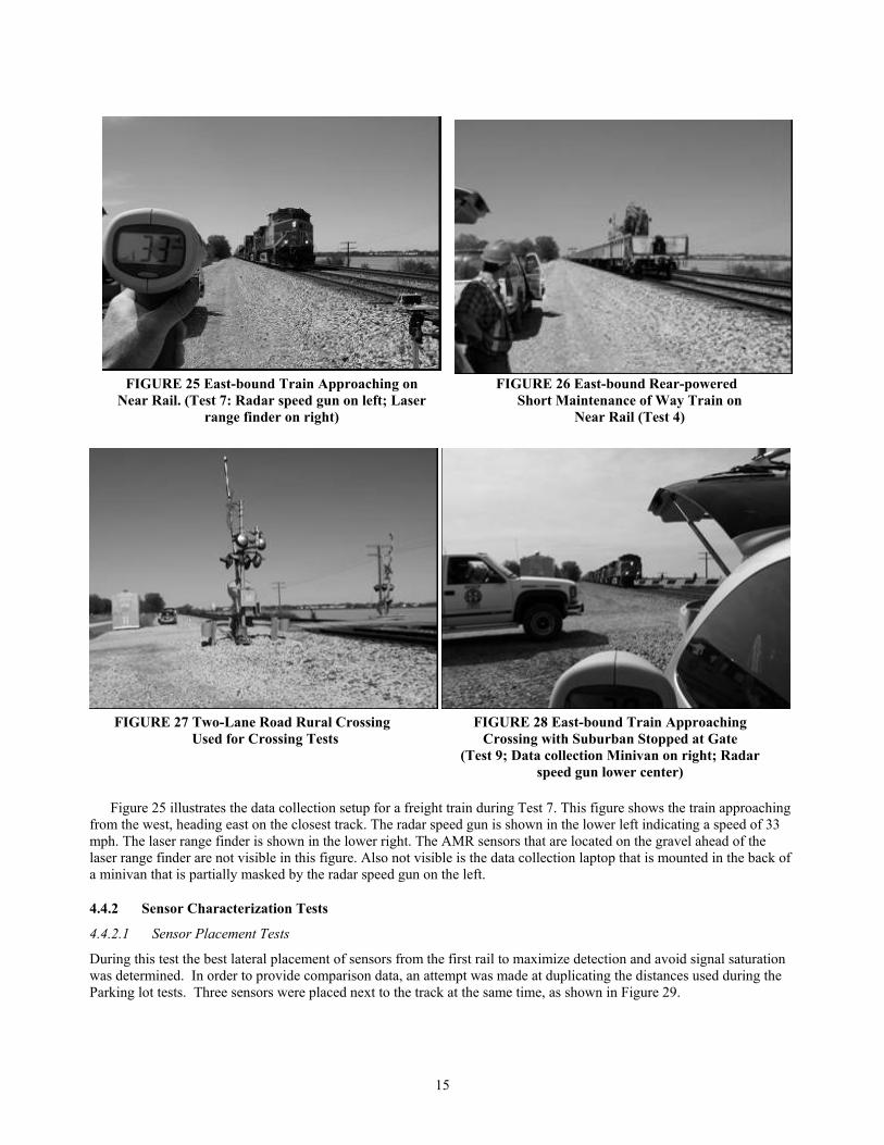
Figure 25 illustrates the data collection setup for a freight train during Test 7. This figure shows the train approaching from the west, heading east on the closest track. The radar speed gun is shown in the lower left indicating a speed of 33 mph. The laser range finder is shown in the lower right. The AMR sensors that are located on the gravel ahead of the laser range finder are not visible in this figure. Also not visible is the data collection laptop that is mounted in the back of a minivan that is partially masked by the radar speed gun on the left.

4.4.2 Sensor Characterization Tests

4.4.2.1 Sensor Placement Tests

During this test the best lateral placement of sensors from the first rail to maximize detection and avoid signal saturation was determined. In order to provide comparison data, an attempt was made at duplicating the distances used during the Parking lot tests. Three sensors were placed next to the track at the same time, as shown in Figure 29.

FIGURE 25 East-bound Train Approaching on Near Rail. (Test 7: Radar speed gun on left; Laser

range finder on right)

FIGURE 26 East-bound Rear-powered Short Maintenance of Way Train on

Near Rail (Test 4)

FIGURE 27 Two-Lane Road Rural Crossing Used for Crossing Tests

FIGURE 28 East-bound Train Approaching Crossing with Suburban Stopped at Gate

(Test 9; Data collection Minivan on right; Radar speed gun lower center)

16

These distances are 5 ft and 18ft. For ease of setup, these distances will be referenced to the closest rail. With a rail separation of 4.7 ft, these distances correspond roughly to 2.5 ft to 15.5 ft from the nearest rail. In addition, a sensor was placed 7.5 ft from the nearest rail corresponding to the detection of a

highway vehicle stopped at a crossing.

Only the Y-Axis data from the placement test is shown in Figure 30. It was determined there was no advantage to placing the sensor either 2.5ft or 15.5ft from the first rail. In order to maintain a consistent sensor placement and to reduce saturating the sensor, the7.5ft distance was chosen for any future detection system.

4.4.2.2 Locomotive Noise Tests

In this test locomotive noise EMI signatures from the locomotive electrical equipment was recorded. Sensors were placed laterally from the center of a GP-39-F that was undergoing maintenance, as illustrated in Figure 31. Two wireless transmitters from two of the sensors can be seen from the two sensors furthest from the locomotive at 7.5ft and

18ft, and 28ft distance from a running and stationary locomotive.

During the first test, the locomotive was idling and hence not charging the locomotive batteries. During the second test, the locomotive was revved up for several minutes to the maximum power, rpm, and load, generating an EMI signature. For this locomotive, the maximum power setting is 2300 Hp. Finally, during the third test, it appears that the engine was revved to a much higher level and held at that rpm just before we stopped taking data. Since the locomotive was never turned off, the EMI measurements were collected relative to the idle setting. The data collection system was located in the back of the minivan.

The EMI data, shown in Figures 32, demonstrates that there is only a low level of EMI at 7.5ft from a powered locomotive. From the X-axis’s calibrated ambient idle level of around 4 mgauss the EMI level changes to 8.5 mgauss during the engine tune up. For comparison, Figure 33 presents the signature of a passing train. Hence, when the 4-5 mgauss EMI signature is compared to a typical locomotive signature (left-hand side of Figure 32) of around 100 mgauss, the locomotive EMI contributes less

TRAIN

SENSORS:

S1

S2

S3

TRAIN

5'

18'7.5'

13.5'

FIGURE 29 Train Signatures vs. Sensor Offset Distance (West <-->East)

Emporia Sensor Placement Test 3 (d) 2.5ft,7.5ft,15.5ft

-10000

-8000

-6000

-4000

-2000

0

2000

4000

39.9

45.1

50.3

55.5

60.7

65.9

71.1

76.3

81.5

86.7

91.9

97.1

102

108

113

118

123

Sec

Cou

nts

y 2.5ft y7.5ft y15.5ft

FIGURE 29 Sensor Placement Test

FIGURE 30 Stationary Locomotive EMI Signature Tests (3 sensors – 2 wireless -- shown offset from

center of locomotive)

17

than 10% of the total signal magnitude.

The conclusion from these EMI tests is that level changes are too small to cause interference with the magnetic signature of the locomotive. In addition, EMI most likely can’t be used to detect an approaching train using magnetometers.

It is important to keep in mind, however, that this was a static locomotive test. As a result, there was no electrical noise being generated from such sources as the traction motor control circuits, commutator noise, etc.

4.4.2.3 Detection Distance Tests

During this test the maximum detection distance of an approaching train was determined. Data from Test 3 Sensor Placement test and Test 5 Speed test was used to determine train distance. A rangefinder was also placed next to the track in order to give digital distance readouts as the train approached.

After taking the time delta between the first z-axis change from ambient at 1300.55sec and the first peak or closest approach to the sensor at 1305sec, the farthest detection distance appears to be 173.55ft, as seen in Figure 34. To compute this distance, the time difference between initial rise in ambient signature to maximum signature was multiplied times the train speed.

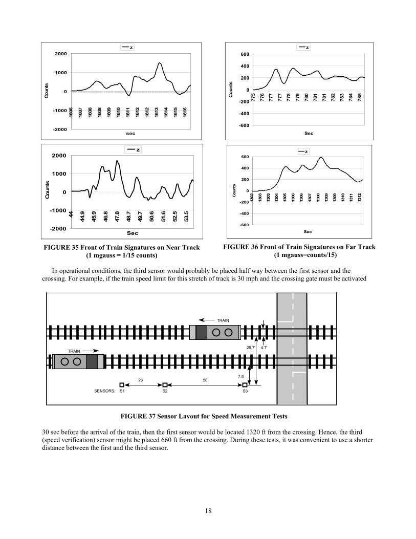
4.4.3 Signature Identification Signature data was recorded during all testing and test configurations. The passing rail vehicle types are listed in Table 2. Figure 35 shows the front end signature of two passing trains on the near track. Figure 36, in turn, shows the front end signature of two passing trains on the far track. As can be seen from these figures, each train has a distinct signature even though all have locomotives in the front that did not appear to be too dissimilar.

4.4.4 Locomotive Speed Test

During this test the speed of passing train was determined using 3 sensors and a radar gun. The sensor layout is shown in Figure 37. Under this concept, as the train passes the each sensor from either direction on one of 2 tracks, the data is transmitted to a computer. The computer determines train speed by taking the arrival time delta between the first two sensors. When the train passes the third sensor in the row for that direction, the computer compares the data arrival time to the second sensor and computes another speed estimate. This second speed estimate is compared to the first speed estimate to verify that the train’s speed has not changed significantly.

Magnitude EMI

4.04.55.05.56.06.57.07.58.08.59.0

0 20 40 60 80 100

120

140

160

180

200

220

240

260

280

Sec

Mill

igau

ss

ENDING APPEARS TO BE HELD AT A HIGH REV.

CALIBRATEDAMBIENT

RETURN TO AMBIENT

ENGINE REVVING

ENGINE REVVING

Magnitude EMI

4.04.55.05.56.06.57.07.58.08.59.0

0 20 40 60 80 100

120

140

160

180

200

220

240

260

280

Sec

Mill

igau

ss

ENDING APPEARS TO BE HELD AT A HIGH REV.

CALIBRATEDAMBIENT

RETURN TO AMBIENT

ENGINE REVVING

ENGINE REVVING

FIGURE 31 Signature during Locomotive EMI Testing

(Ambient at idle, engine revved up to max power, max load, and max rpm).

Magnitude Train 1 passing on Near track

050

100150200250300350400450500

1605

1610

1615

1620

1625

1630

1636

1641

1646

1651

1656

1661

1666

1671

1676

Sec

Mill

igau

ss

FIGURE 32 Signature of a Passing Train

Train 3 passing on Far track

1305,1.463

1279.75, 0.426

1300.55, 0.418

0.25

0.45

0.65

0.85

1.05

1.25

1.45

1.65

1263

1266

1269

1272

1275

1278

1281

1284

1287

1290

1292

1295

1298

1301

1304

1307

1310

1313

1316

1319

1322

1325

Sec

Millig

auss

PEAK TIME

Log Magnitude

AMBIENT

Train 3 passing on Far track

1305,1.463

1279.75, 0.426

1300.55, 0.418

0.25

0.45

0.65

0.85

1.05

1.25

1.45

1.65

1263

1266

1269

1272

1275

1278

1281

1284

1287

1290

1292

1295

1298

1301

1304

1307

1310

1313

1316

1319

1322

1325

Sec

Millig

auss

PEAK TIME

Log Magnitude

AMBIENT

FIGURE 33 Detection Distance Data

18

In operational conditions, the third sensor would probably be placed half way between the first sensor and the crossing. For example, if the train speed limit for this stretch of track is 30 mph and the crossing gate must be activated

30 sec before the arrival of the train, then the first sensor would be located 1320 ft from the crossing. Hence, the third (speed verification) sensor might be placed 660 ft from the crossing. During these tests, it was convenient to use a shorter distance between the first and the third sensor.

-2000

-1000

0

1000

2000

1606

1607

1608

1608

1609

1610

1611

1612

1612

1613

1614

1615

1616

sec

Cou

nts

z

-2000

-1000

0

1000

2000

44

44.9

45.9

46.8

47.8

48.7

49.7

50.6

51.6

52.5

53.5

Sec

Cou

nts

z

FIGURE 35 Front of Train Signatures on Near Track

(1 mgauss = 1/15 counts)

FIGURE 37 Sensor Layout for Speed Measurement Tests

TRAIN

SENSORS: S1 S2 S3

TRAIN

50'7.5'

25'

25.7' 4.7'

-600

-400

-200

0

200

400

600

775

776

777

777

778

779

780

781

781

782

783

784

785

Sec

Cou

nts

z

-600

-400

-200

0

200

400

600

1302

1303

1303

1304

1305

1306

1306

1307

1308

1309

1309

1310

1311

1312

SecC

ount

s

z

FIGURE 36 Front of Train Signatures on Far Track

(1 mgauss=counts/15)

19

The speed calculation involves dividing the sensor separation distance by the time delta between two sensors. As a result, the accuracy of the speed measurement depends directly on the separation distance and scales as the fraction of the time delta measurement accuracy to the time delta. As a result, the larger the separation distance, the smaller the speed measurement error if the speed does not change during this measurement interval. Similarly, the finer the time measurement resolution (the higher the data rate), the more accurate the speed measurement. It is assumed that both sensors are using the same clock or synchronized clocks to record the time of closest approach, shown in Figure 38.

While the data for the sensors was 20 Hz (0.05 sec time resolution), the sensor clock times were only synched to the nearest second. As a result, a method had to be found to determine the

clock synch time bias between two sensors.

One of the tests involved the recording of three trains that passed the sensors in a short period of time. Hence, the DAQ did not stop recording data until all three trains had passed. The radar speed measurement and time deltas for one of the trains was used to determine the clock synch time biases for a second train. These biases were then applied to the time deltas for the second train to

determine the speed.

Shown in Figures 39 and 40 are two of the trains used during the speed test as well as the radar gun readings. Focusing on the time delta between S1 and S3, separated by 75 ft, an estimated speed of 28.4 mph was computed. This is

within 5% of the speed gun value of 30 mph.

The nominal time for Train 3 to travel 75 ft is 1.70 sec. With a time resolution of 0.05 sec, the time resolution error contribution is 0.9 mph, accounting for 3% of this error. In addition, there is a 1% speed gun measurement error, according to the manufacturer.

FIGURE 41 Street Crossing Sensor Measurement Configurations

(S1 & S2 for crossing island monitoring; S3 for quadrant location determination)

CAR

S2

S3

TRAIN

SENSORS:

S1

FIGURE 39 Emporia Test 8B Train 2 FIGURE 40 Emporia Test 8C Train 3

Train 2 Speed testEmporia test 8B (Ti) Delta of M1,M2, M3

Train 2 passing on far track

777.05

773.45

774.3

-100

0

100

200

300

400

770

771

773

774

775

776

778

779

780

782

783

784

786

787

788

789

Sec

Cou

nts

z1 z2 z3

FIGURE 38 Train 2 Vertical Axis Time of Closest Approach (3 Sensors; Train is moving east to west)

20

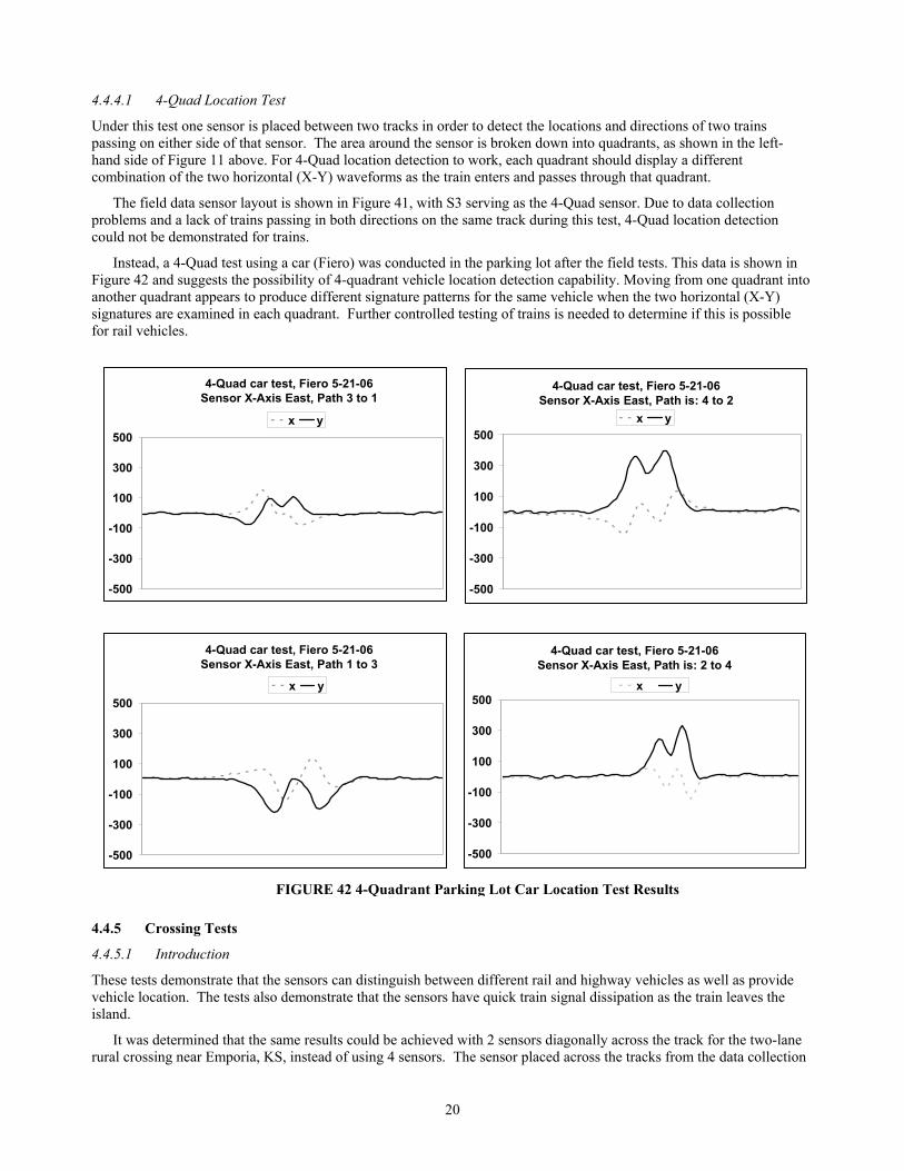
4.4.4.1 4-Quad Location Test

Under this test one sensor is placed between two tracks in order to detect the locations and directions of two trains passing on either side of that sensor. The area around the sensor is broken down into quadrants, as shown in the left-hand side of Figure 11 above. For 4-Quad location detection to work, each quadrant should display a different combination of the two horizontal (X-Y) waveforms as the train enters and passes through that quadrant.

The field data sensor layout is shown in Figure 41, with S3 serving as the 4-Quad sensor. Due to data collection problems and a lack of trains passing in both directions on the same track during this test, 4-Quad location detection could not be demonstrated for trains.

Instead, a 4-Quad test using a car (Fiero) was conducted in the parking lot after the field tests. This data is shown in Figure 42 and suggests the possibility of 4-quadrant vehicle location detection capability. Moving from one quadrant into another quadrant appears to produce different signature patterns for the same vehicle when the two horizontal (X-Y) signatures are examined in each quadrant. Further controlled testing of trains is needed to determine if this is possible for rail vehicles.

4.4.5 Crossing Tests

4.4.5.1 Introduction

These tests demonstrate that the sensors can distinguish between different rail and highway vehicles as well as provide vehicle location. The tests also demonstrate that the sensors have quick train signal dissipation as the train leaves the island.

It was determined that the same results could be achieved with 2 sensors diagonally across the track for the two-lane rural crossing near Emporia, KS, instead of using 4 sensors. The sensor placed across the tracks from the data collection

FIGURE 42 4-Quadrant Parking Lot Car Location Test Results

4-Quad car test, Fiero 5-21-06Sensor X-Axis East, Path is: 4 to 2

-500

-300

-100

100

300

500x y

4-Quad car test, Fiero 5-21-06Sensor X-Axis East, Path is: 2 to 4

-500

-300

-100

100

300

500x y

4-Quad car test, Fiero 5-21-06Sensor X-Axis East, Path 3 to 1

-500

-300

-100

100

300

500x y

4-Quad car test, Fiero 5-21-06Sensor X-Axis East, Path 1 to 3

-500

-300

-100

100

300

500x y

21

laptop was linked using radio modems as was the 3rd sensor placed between the 2 mainline tracks to collect 4-quadrant data.

4.4.5.2 Gate Cross Traffic Test

Under this test, vehicle locations were referenced to the rail and crossing gate. The location of highway vs. rail vehicles was determined as both vehicles approached the crossing, as shown in Figure 41. The signatures seen at a crossing before, during, and after train arrival was analyzed. The effect that a train signature had on a highway vehicle signature was to saturate or mask it, but not until the train was almost next to the sensor. This allows the observation of car movements up to the point were the train is next to the sensor.

Test results in Figure 43 show a non-test car (compact) passing S1 at around 63sec just before the SUV approaches and waits. The vertical axes are clipped to highlight the vehicle signatures. As a result, the train signature is not fully displayed. The X-axis is aligned parallel to the tracks, the Y-axis is perpendicular to the tracks, and the Z-axis points up.

As the compact passes the SI sensor, the classical sine-wave pattern is seen in the Y-axis with a corresponding spike in the X-axis. The SUV is approaching at around 112sec and doesn’t produce any of these effects nor does one see these during its reversal away from the track at around 360sec.

Vehicle information is masked by the train signature when the train arrives at around 167sec and remains masked until its departure at around 340sec.

Once the train arrives it is too late to stop a vehicle from entering the island. Hence, vehicle information is not needed again until the train passes. The gate should have been activated 20-30 seconds before train arrival.

One possible warning system might look for the entry sine-wave into the island and verify either an exit sine-wave from the cross sensor or a reversal back across the island to the vehicles entry point. In the latter case, a reverse sine-wave (mirror image pattern) at the first sensor should be observed. If neither of these is seen, then the vehicle is still sitting in the island on the tracks and the exit gates, of a 4-quad crossing gate system, need to be raised.

Note the similarities of these results to the parking lot test results in Figure 24. The same increase is seen as a vehicle approaches and waits at the gate. A real train produces a much larger increase as it enters and passes through the island perpendicular to the waiting vehicle.

A second test was performed with the SUV and an approaching train, as illustrated in Figure 44, for the S1 sensor. The SUV approaches at 70sec is shown along with its entry into the island at about 240sec. Note that there is no sine-wave at the beginning when the SUV approaches and waits, but there is one after the train signal ends, indicating the SUV entry into the island.

These same results are shown for the S2 sensor in Figure 45. This figure shows the SUV approach and sit across the island as seen at around 68sec. At this time, the X & Y-axis signatures flatten and the Z-axis signature spikes down and flattens. At about 245sec one sees the SUV pass sensor S2 via the classical sine-wave pattern. Since S2 is located 7.5ft in front of the first rail of the second track (See Figure 41), it can be determined that the SUV is no longer in the island.

FIGURE 43 Test 1, Mag 1 Plots of Compact, SUV, and Passing Train at Emporia, KS, Rural Crossing

(Vertical axes are clipped to highlight vehicle signatures – maximum train signatures not fully displayed)

22

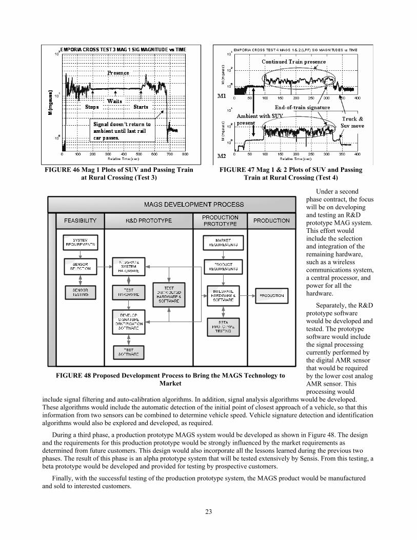
Two tests were performed that explored the detection of stopped rail cars in the crossing island and the end of the train through the island. During Test 3, shown in Figure 46, a train stopped and waited on the far track as S1 detected its continued presence shown in X, Y, Z, and magnitude plots. Additionally, the trains can be seen stopping in the crossing at around 200sec demonstrated by a lack of signal deflection. It then starts moving again just past 500sec demonstrated by the resumption of signal deflection.

During Test 4, shown in Figure 47, a train passed through the crossing without stopping. Verification of a continued train presence indication was also seen during this test that used the same sensor configuration as Test 3.

Both tests show a continued large a reading that is either above or below ambient until the train has passed the sensor. This verification would determine that ambient readings are reached for both sensors after the train has left the island. To verify the train has completely left the island a comparison needs to be made between measurements from S1 and from the cross track sensor S2, shown in Figure 45. A more detailed verification could be made by comparing signal shape seen by the first sensor with the signal shape seen by the second sensor. The second sensor should see roughly the same shape except delayed in time, as seen in Figure 47.

4.5 PLANS FOR IMPLEMENTATION

The intent of this feasibility study is to verify that the key technology is feasible for reliable and practical crossing gate activation systems. Hence, as shown in Figure 48, the feasibility study has focused on the AMR magnetometer sensor.

FIGURE 44 Test 2, Mag 1 Plots of SUV, and Passing Train at Emporia, KS, Rural Crossing (Vertical axes are clipped to highlight vehicle signatures – maximum train signatures not fully displayed)

FIGURE 45 Test 2, Mag 2 Plots of SUV, and Passing Train at Emporia, KS, Rural Crossing (Vertical axes are clipped to highlight vehicle signatures – maximum train signatures not fully displayed)

23

Under a second phase contract, the focus will be on developing and testing an R&D prototype MAG system. This effort would include the selection and integration of the remaining hardware, such as a wireless communications system, a central processor, and power for all the hardware.

Separately, the R&D prototype software would be developed and tested. The prototype software would include the signal processing currently performed by the digital AMR sensor that would be required by the lower cost analog AMR sensor. This processing would

include signal filtering and auto-calibration algorithms. In addition, signal analysis algorithms would be developed. These algorithms would include the automatic detection of the initial point of closest approach of a vehicle, so that this information from two sensors can be combined to determine vehicle speed. Vehicle signature detection and identification algorithms would also be explored and developed, as required.

During a third phase, a production prototype MAGS system would be developed as shown in Figure 48. The design and the requirements for this production prototype would be strongly influenced by the market requirements as determined from future customers. This design would also incorporate all the lessons learned during the previous two phases. The result of this phase is an alpha prototype system that will be tested extensively by Sensis. From this testing, a beta prototype would be developed and provided for testing by prospective customers.

Finally, with the successful testing of the production prototype system, the MAGS product would be manufactured and sold to interested customers.

FIGURE 48 Proposed Development Process to Bring the MAGS Technology to

Market

FIGURE 47 Mag 1 & 2 Plots of SUV and Passing Train at Rural Crossing (Test 4)

FIGURE 46 Mag 1 Plots of SUV and Passing Train at Rural Crossing (Test 3)

24

5 REVIEW PANEL INPUT The following summarizes input from the Review Panel, based on the Stage 1 Briefing as well as the Stage 4 Final Briefing and Final Report. The Review Panel’s feedback during the Stage 1 Briefing was utilized to guide and structure the lab and field testing.

5.1 STAGE 1 REVIEW PANEL FEEDBACK

The Stage 1 Briefing was held via teleconference from Campbell CA. on Wednesday, 9 November, 10:30 AM - 12:00 PM. The Review Panel members who participated included: Chuck Taylor/TRB, Jim Smailes/FRA, Pete Mills/HWA, Corey Wills/ BNSF, and Richard Reiff/ TTCI.

It was suggested that our field tests should follow some test guidelines, possibly defined by some regulatory committee. In response to this suggestion we attempted to model our test matrix after what was done in past TTCI testing of crossing warning sensor systems. There was a discussion centered on philosophical differences between those tests and the ones that we have proposed. In essence, the review panel took a top-down application-focused approach. We, in turn, were taking a bottoms-up (what can the sensor do) sensor-focused approach. Based on this feedback, we decided to incorporate both approaches in order to thoroughly cover all the details.

Feedback was also given for our proposed parking lot and railroad testing. Suggestions were made that we should not limit ourselves to cars but should also measure trucks, such as an 18-wheeler sitting next to the sensor. It was not practical to test this type of vehicle at this time. Since the detection system sensors would most likely be placed in all four corners of a crossing as well as some distance from the road, it was felt that a large truck would not inhibit detection of other vehicles by at least one of the four sensors.

Another suggestion was to take measurements next to a locomotive under full load. This data would be used to determine whether any electro-magnetic interference (EMI) generated by the locomotive electrical systems could be measured and whether this would interfere with the locomotive magnetic signature. This test was incorporated into our test matrix. An additional suggestion was to contact Honeywell to see what EMI data they have relative to their AMR sensors. Honeywell would not provide this type of data, when requested.

Corey Wills of the BNSF, located in Topeka, KS, was asked to help us in performing the rail-yard field tests. He agreed and was a vital part of setting up this test location as well as being an active participant in our field testing. In addition, he shared with us his past experience with the data acquisition (DAQ) software from Agilent Technologies and how it performed relative to other competing software.

The Panel also pointed out to us the high cost of using long cable runs to connect remote (along-track) sensors with a central processor near the crossing. Hence, it was determined that cables would be replaced with wireless data modems.

A question was also raised on how the gate warning activation system would use the magnetometer information after vehicle detection had been established. Specifically, would this information be used to open/close gates or just activate warning systems? Current systems can do both. Also, what are the system failure options? The preferred failure mode could mimic the current system fail mode approach and automatically lower the entry gates and raise the exit gates of a four-quadrant crossing gate system.

5.2 STAGE 4 FINAL BRIEFING FEEDBACK

The final briefing and telecom was held Thursday, 22 June, at 10 AM – 12PM in Washington, DC. Members of the Review Panel who participated were: Chuck Taylor/TRB, Pete Mills/ FHWA, Corey Wills/ BNSF, and Rich Reiff/ TTCI-AAR. The last 3 participated by telecom.

A discussion took place about EMI interference from overhead power lines and ground return paths in the case of electric transit rail vehicles. One panelist mentioned that there are shielding antennas that could attach to mag sensors to minimize EMF. It was decided that this would not be practical for the magnetometer sensors since these antennas could mask the earth magnetic field used by the sensors.

Another question that was raised is what can a crossing system do with the information that a vehicle is stuck in the crossing island? The problem is that such a warning has to be received by a train minutes in advance in order for the train to come to a safe stop. Currently, however, warning systems are activated 20-30 sec prior to the arrival of a train. It was concluded that the most practical use for this information would be to raise the exit gate of a four-quadrant crossing gate system to allow the vehicle to exit the island, if it can.

25

It was further brought to our attention that a future detection system based on this concept will need its software and hardware to sense, interpret, and react to a train departure (raise the gates) in less than 2 seconds after the train clears the crossing in order to be competitive with the existing system. It was further suggested that we included a 2-second release test during future testing. Since this type of magnetometer responds instantly to changes in the magnetic field, we feel that the 2-second requirement is obtainable.

6 SUMMARY AND CONCLUSIONS

6.1 GOALS DEMONSTRATED

6.1.1 Vehicle Detection and Identification:

It appears each train has its own signature that can be used as a unique identifier. More research would be needed in order to verify how this would be utilized and ensure that other trains don’t have similar patterns. These unique signatures were observed even for the front of trains where the locomotive signatures would be expected to be somewhat similar.

Street vehicles don’t produce a good signature when passing by the sensor. If there is a need to distinguish one vehicle from another then an alternative sensor location will be needed. In this case, sensors could be installed in the middle of the road along both directions in order to record each vehicle’s unique signature as it passes over the sensors. This information could be used to help distinguish one vehicle from another: bus vs. large truck, or truck vs. large car. Additionally, this sensor arrangement could be utilized in determining the approaching vehicle speed.

6.1.2 Locomotive Noise Interference Signature:

The electromagnetic noise of a locomotive under full load doesn’t appear to have a large magnitude. Therefore, it shouldn’t create interference with locomotive detection. The noise magnitude appears to be less than 10% of the total (magnetic and noise) signature.

6.1.3 Four-Quadrant Train Location:

Since there were a limited number of trains passing the sensor during 4-quadrant field tests, a full determination of this capability could not be made. The problem is that the train signature is very complex, and hence care must be taken to focus only on the signal from the lead locomotive. This capability was demonstrated in the lab with simple metal objects and in the parking lot with a car.

6.1.4 Detection of Rail Cars Left in Crossing:

Field tests demonstrated that the sensors can detect both rail cars and street vehicles entering and exiting the island. This detection could either focus on a large signal magnitude increase or the classical sine-wave pattern given as the vehicle passes the sensor. Rail cars, because of their large mass, will easily be detected if they remain in the crossing, creating a large signal magnitude plateau.

Street vehicles appear to be detectable by either or both the nearest sensor and the cross-track sensor. They will also be detected when passing the near sensor as they enter the crossing and by the cross-track sensor as they exit the island. They will appear as stopped in the crossing island, if they enter and don’t reverse past the sensor again, creating a mirror image signal. Alternately, they will appear to be stopped if they aren’t detected exiting past the cross-track sensor. In either case, deployment of the exit gates of a 4-quadrant crossing gate system could be delayed in order to let them exit.

6.1.5 Signature Repeatability:

Since these were passive tests and each train could not be moved past the sensor repeatedly, train signature repeatability could not be fully determined at this time. Additional analysis on the locomotive signatures at the front of the trains will be able to verify repeatability. Signature repeatability however was observed when two different cars were driven over a sensor multiple times, both forwards and reverse.

26

6.2 SENSOR LIMITATIONS

6.2.1 AMR Sensor Selection

It was discovered during the Stage 1 sensor review that Honeywell is the only manufacturer of complete AMR sensors. According to their sensor expert, there are companies in Europe that make the sensing element, but don’t provide the supporting electronic circuitry for a complete sensor. The Honeywell sensors can be purchased as analog or digital sensors. The digital AMR magnetometers are available as 1, 2, or 3 axis (X, Y, and Z) sensors.

As an alternative supplier, a European company making the AMR sensing elements could be used. The additional detector circuitry could be added to these sensing elements from a 3rd party electronics company.

6.2.2 Analog AMR Sensors

Almost all of the tests were performed with four digital 3-axis AMR magnetometers. In addition, the corresponding 3-axis analog AMR magnetometers were also investigated in the lab.

In general, the analog sensors produced much noisier measurements than the digital sensors. It was found that the analog sensors required more extensive work before they could be used as functional testing devices than was earlier thought. Additional circuitry was needed for: anti-aliasing filters, magnetic offsets for all three axes, and degaussing circuitry to degauss the sensor heads.

The analog sensors also detected a noise at 60Hz from the electrical outlets. This noise was about 500µv peak-peak. This is still much higher than the 40µv detection level, which means detection below 500µv isn’t possible until this noise is eliminated.

6.2.3 Digital AMR Sensors

The digital sensors showed similar noise levels. However, they can use their internal CPU’s auto averaging feature to low pass filter the signal and remove most, if not all, of the noise.

For a production MAGS system, an analog sensor would probably be used due to its lower cost. This sensor would then have additional circuits installed to perform the same functions as are currently performed in the digital sensor. This would still, potentially, be a lower cost solution than basing a production system on the digital sensor.

In general, it was found that the AMR sensors drift with temperature changes. This can be minimized by periodic auto-calibrations that reset the current ambient readings back to zero.

The sensors are also very sensitive to their installed orientation. Hence, they need to be installed in a fixed location that is not susceptible to vibration. During the field testing there did not appear to be much vibration interference caused by passing trains. Train and street vehicle detection was possible during all our testing and at no time did vibration block or mask any vehicle. During the 2.5ft placement test from the first rail only few nonsensical data points were detected out of several minutes of data collected at 20Hz. This could have been less vibration and more slippage of the sensors since they were not firmly mounted to the ground. Further investigation of the vibration issue is needed to determine what (if any) effect it will have on detecting rail vehicles. Nonsensical vibration data can be treated the same way as lightning. The software can determine what is happening before and after this signal, compare this finding with any nearby sensors and adjust its detection method.

Since these sensors cannot distinguish between magnetic and electromagnetic disturbances to the ambient earth magnetic field, they are sensitive to electromagnetic interference. The specific case where this was observed was for an electric light rail train. For this train, the variable current (from the train) in the overhead power lines could be detected before the magnetic signature of the train was detected. However, the electromagnetic signature was considerably different from the magnetic signature of the train when all three axes of the magnetometer signal were examined.

6.3 CONCLUSIONS

Overall, the results from this study established the feasibility of using digital AMR magnetometers for train detection and speed determination. In addition, the feasibility for using these sensors for vehicle detection near a crossing and within the crossing island was determined. Finally, the sensors can also be used to detect hi-rail vehicles, which currently have insulated wheels, on the tracks, as well as the last rail car of a passing train.

The sensors can determine the unique signatures of vehicles. These signatures can be used to distinguish different vehicles or separate vehicles from background electro-magnetic interference. In addition, the sensors can determine

27

whether a vehicle has stopped or changed direction. By using the 3-axis digital AMR magnetometers, their sensitivity to any change in the orientation of the sensor after installation is minimized.

Hence, based on this feasibility study, the AMR magnetometer provides a robust and flexible alternative sensor system for activating crossing warning systems over the current use of track circuits. It is therefore recommended that further work is funded for the development and testing of an R&D prototype AMR magnetometer-based crossing warning system. This prototype system would combine all the hardware of an operational system, including a central processor, wireless communications system, and power sources for the sensors. In addition, this prototype would include the development and testing of the algorithms for automatic vehicle detection, bias calibration, speed determination, and crossing arrival time determination.

7 REFERENCES 1. Anon, “HMC2003 Three-Axis Magnetic Sensor Hybrid”, Honeywell (Stage 1)

2. Anon, “HMR2300 Smart Digital Magnetometer”, Honeywell (Stage 1)

3. Anon, “Vehicle Detection Using AMR Sensors,” Honeywell Application Note – AN218, August 2005

4. Anon, “Evaluation of Alternative Detection Technologies for Trains and Highway Vehicles at Highway Rail Intersections”, 1999, Richard P. Reiff and Scott E. Gage of TTCI, Anya A. Carroll and Jeffrey E. Gordon of Volpe Center.