magnetic resonance with quantum microwaves
TRANSCRIPT

HAL Id: tel-01496176https://tel.archives-ouvertes.fr/tel-01496176
Submitted on 27 Mar 2017
HAL is a multi-disciplinary open accessarchive for the deposit and dissemination of sci-entific research documents, whether they are pub-lished or not. The documents may come fromteaching and research institutions in France orabroad, or from public or private research centers.
L’archive ouverte pluridisciplinaire HAL, estdestinée au dépôt et à la diffusion de documentsscientifiques de niveau recherche, publiés ou non,émanant des établissements d’enseignement et derecherche français ou étrangers, des laboratoirespublics ou privés.
Magnetic resonance with quantum microwavesAudrey Bienfait
To cite this version:Audrey Bienfait. Magnetic resonance with quantum microwaves. Quantum Physics [quant-ph]. Uni-versité Paris-Saclay, 2016. English. NNT : 2016SACLS297. tel-01496176

NNT : 2016SACLS297
En cas de cotutelle, mettre ici le logo de l’établissement de préparation de la thèse
THESE DE DOCTORAT DE
L’UNIVERSITE PARIS-SACLAY PREPAREE A
L’UNIVERSITE PARIS-SUD
ECOLE DOCTORALE N° 564 Physique de l’Ile de France
Spécialité de doctorat : Physique
Par
Audrey Bienfait
MAGNETIC RESONANCE WITH QUANTUM MICROWAVES
réalisée dans le groupe QUANTRONIQUE
SPEC - CEA SACLAY France
Thèse présentée et soutenue à Gif-sur-Yvette, le 14 octobre 2016. Composition du Jury : Président (à préciser après la soutenance)
Prof. Jean-François Roch Laboratoire Aimé-Cotton Président du Jury Prof. Gunnar Jeschke ETH Zürich Rapporteur Prof. Wolfgang Wernsdorfer Institut Néel Rapporteur Prof. Michel Pioro-Ladrière Université de Sherbrooke Examinateur Prof. Andreas Wallraff ETH Zürich Examinateur Dr. Patrice Bertet SPEC, CEA-Saclay Directeur de thèse

A papa,c’est une grande joie que d’avoir marché (un petit peu) dans tes pas.
ii

Remerciements
Beaucoup de personnes ont contribué à rendre ces trois années et demie passées dans le groupeQuantronique formidables et inoubliables, et je voudrais par ces quelques mots les remercier toutestrès chaleureusement.
Il y a en premier ceux que j’ai cotoyés tous les jours et qui m’ont appris énormément. Merci toutd’abord à Patrice, pour ta disponibilité, ton incroyable clarté, ton optimisme et ta très grandegentillesse qui ont fait de ces mois passés au labo et à rédiger ce mémoire des moments chouettes,certes très riches en physique, parfois frustrants, mais aussi remplis d’enthousiasme et captivants!Si Patrice m’a appris la physique, c’est bien Yui que je dois remercier pour m’avoir appris bien destechniques expérimentales et de nano-fabrication (ainsi que de la mécanique!). Je n’aurais pas puavoir un prof plus sympa, patient et rigoureux tout à la fois !Merci aux permanents de Quantronique (au sens large): Carles, Cristian, Daniel, Denis, Fabien,Hélène, Hugues, Marcelo, Pascal, Philippe, et Pief, d’être aussi passionnés et passionnants, et d’avoirété aussi disponibles pour discuter, filer des coups de main et des encouragements.Merci à la jeune génération qui a garanti la bonne ambiance à table, au labo et en-dehors: mesprédécesseurs Cécile, Olivier, et Vivien, les post-docs Xin, Michael, Sebastian, Philippe, Simon,Caglar, Marc et Leandro, mes co-thésards et « compagnons de rédaction » Kristinn (could not havepicked a better office and car mate!), Camille, Pierre et Chloé, et enfin les tous derniers arrivantsBartolo et Fernanda.Merci à ceux qui ont rendu possible cette thèse. Merci à l’atelier mécanique, Dominique, Jean-Claude et Vincent d’avoir réalisé toutes nos pièces même si elles étaient coriaces. . . Merci à l’atelierde cryogénie, Patrick, Philippe et Matthieu, les héros qui ont sauvé le cryostat (deux fois!) d’unesituation plus que précaire; merci au secrétariat et à la direction du SPEC.
Il y a ensuite tous ceux qui ont contribué directement aux expériences qui sont présentées ici etavec qui j’ai interagi avec beaucoup de plaisir. Merci à toute l’équipe de Londres, Jarryd, Gary, Evaet John Morton, qui nous ont fait découvrir ce sacré champion de bismuth, « the new black stuff», et qui nous ont apporté tant d’idées fructueuses. Merci aussi à Klaus Mølmer, Brian Julsgaardet Alexander Holm-Kiilerich, nos collaborateurs théoriciens d’Aarhus, avec qui ce fut un plaisirde travailler par quelque moyen que ce soit (après avoir essayé Skype, Hangouts, RendezVous etautres, nous concluons d’ailleurs que le téléphone reste sacrément pratique!).
Finalement, je voudrais remercier ma famille, absents comme présents, et mes amis, pour leurencouragements et pouvoir avoir été là. Merci surtout à Félix, de m’avoir soutenue et supportéedans les moments difficiles, et d’avoir accepté mes horaires parfois incongrus, qui nous ont menés àcommander bien trop de pizzas !
iii

Contents
Remerciements iii
Résumé détaillé 1
1 Introduction 111.1 Circuit quantum electrodynamics for magnetic resonance . . . . . . . . . . . . . . . . 111.2 Quantum microwaves and spin dynamics . . . . . . . . . . . . . . . . . . . . . . . . . 121.3 Electron spin resonance at the quantum-limit of sensitivity . . . . . . . . . . . . . . . 141.4 The Purcell effect applied to spins . . . . . . . . . . . . . . . . . . . . . . . . . . . . . 171.5 Squeezing-enhanced magnetic resonance . . . . . . . . . . . . . . . . . . . . . . . . . 18
I Background 20
2 Quantum circuits and quantum noise 212.1 Quantum microwaves and quantum circuits . . . . . . . . . . . . . . . . . . . . . . . 21
2.1.1 Quantum description of an electromagnetic mode : quantum noise and quan-tum states . . . . . . . . . . . . . . . . . . . . . . . . . . . . . . . . . . . . . . . 21
2.1.2 Lumped element LC resonator . . . . . . . . . . . . . . . . . . . . . . . . . . . 252.1.3 Lossless transmission line . . . . . . . . . . . . . . . . . . . . . . . . . . . . . . 262.1.4 Probing and characterizing a resonator . . . . . . . . . . . . . . . . . . . . . . 29
2.2 Amplification at the quantum-limit . . . . . . . . . . . . . . . . . . . . . . . . . . . . . 332.2.1 Input-output relations for linear amplifiers . . . . . . . . . . . . . . . . . . . . 332.2.2 Quantum limits on the noise added by the amplifier . . . . . . . . . . . . . . . 352.2.3 The flux-pumped Josephson Parametric Amplifier . . . . . . . . . . . . . . . . 36
3 Spins in a cavity 403.1 Spin dynamics in a classical microwave field . . . . . . . . . . . . . . . . . . . . . . . 40
3.1.1 Coherent spin evolution . . . . . . . . . . . . . . . . . . . . . . . . . . . . . . . 403.1.2 Relaxation and decoherence . . . . . . . . . . . . . . . . . . . . . . . . . . . . . 423.1.3 Inductive detection of magnetic resonance . . . . . . . . . . . . . . . . . . . . 43
3.2 Spin dynamics in a quantum microwave field . . . . . . . . . . . . . . . . . . . . . . . 443.2.1 One spin coupled to a harmonic oscillator . . . . . . . . . . . . . . . . . . . . . 453.2.2 Collective effects . . . . . . . . . . . . . . . . . . . . . . . . . . . . . . . . . . . 50
4 Bismuth donors in silicon 544.1 A substitutional donor in silicon . . . . . . . . . . . . . . . . . . . . . . . . . . . . . . 55
4.1.1 Electronic states . . . . . . . . . . . . . . . . . . . . . . . . . . . . . . . . . . . . 554.2 Spin levels and ESR-allowed transitions. . . . . . . . . . . . . . . . . . . . . . . . . . . 584.3 Donors in strained silicon . . . . . . . . . . . . . . . . . . . . . . . . . . . . . . . . . . 634.4 Relaxation times . . . . . . . . . . . . . . . . . . . . . . . . . . . . . . . . . . . . . . . . 64
4.4.1 T1 relaxation . . . . . . . . . . . . . . . . . . . . . . . . . . . . . . . . . . . . . . 644.4.2 Coherence times . . . . . . . . . . . . . . . . . . . . . . . . . . . . . . . . . . . 67
4.5 Optical transitions via donor-bound exciton states . . . . . . . . . . . . . . . . . . . . 694.6 Fabrication . . . . . . . . . . . . . . . . . . . . . . . . . . . . . . . . . . . . . . . . . . . 69
iv

II Magnetic resonance at the quantum limit 71
5 Design and realization of a spectrometer operating at the quantum limit of sensitivity 725.1 Nanoscale ESR . . . . . . . . . . . . . . . . . . . . . . . . . . . . . . . . . . . . . . . . . 72
5.1.1 State-of-the-art . . . . . . . . . . . . . . . . . . . . . . . . . . . . . . . . . . . . 725.1.2 Pulsed inductive detection at the nanoscale . . . . . . . . . . . . . . . . . . . . 73
5.2 Experimental setup . . . . . . . . . . . . . . . . . . . . . . . . . . . . . . . . . . . . . . 775.2.1 Low-temperature operation . . . . . . . . . . . . . . . . . . . . . . . . . . . . . 775.2.2 Room-temperature setup . . . . . . . . . . . . . . . . . . . . . . . . . . . . . . 795.2.3 JPA characterization . . . . . . . . . . . . . . . . . . . . . . . . . . . . . . . . . 79
5.3 Design of a superconducting ESR resonator with high quality factor and small modevolume . . . . . . . . . . . . . . . . . . . . . . . . . . . . . . . . . . . . . . . . . . . . . 825.3.1 Design choices . . . . . . . . . . . . . . . . . . . . . . . . . . . . . . . . . . . . 825.3.2 Electromagnetic simulations . . . . . . . . . . . . . . . . . . . . . . . . . . . . 855.3.3 Coupling to bismuth donor spins . . . . . . . . . . . . . . . . . . . . . . . . . . 855.3.4 Experimental implementation . . . . . . . . . . . . . . . . . . . . . . . . . . . 88
6 ESR spectroscopy of Bismuth donors in silicon 926.1 Hahn-echo detected ESR . . . . . . . . . . . . . . . . . . . . . . . . . . . . . . . . . . . 92
6.1.1 Experimental techniques . . . . . . . . . . . . . . . . . . . . . . . . . . . . . . . 926.1.2 Hahn-echo sequence . . . . . . . . . . . . . . . . . . . . . . . . . . . . . . . . . 936.1.3 Rabi oscillations . . . . . . . . . . . . . . . . . . . . . . . . . . . . . . . . . . . . 94
6.2 Strain-broadened transitions . . . . . . . . . . . . . . . . . . . . . . . . . . . . . . . . . 976.2.1 Doublet-shaped transitions . . . . . . . . . . . . . . . . . . . . . . . . . . . . . 986.2.2 Rabi frequency dependence on B0 . . . . . . . . . . . . . . . . . . . . . . . . . 996.2.3 Induced strain, a likely suspect . . . . . . . . . . . . . . . . . . . . . . . . . . . 101
6.3 Relaxation times . . . . . . . . . . . . . . . . . . . . . . . . . . . . . . . . . . . . . . . . 1036.3.1 Energy relaxation . . . . . . . . . . . . . . . . . . . . . . . . . . . . . . . . . . . 1036.3.2 Coherence times . . . . . . . . . . . . . . . . . . . . . . . . . . . . . . . . . . . 104
7 Spectrometer sensitivity 1057.1 Determining the number of spins . . . . . . . . . . . . . . . . . . . . . . . . . . . . . . 105
7.1.1 Direct counting of the donors . . . . . . . . . . . . . . . . . . . . . . . . . . . . 1057.1.2 Estimate based on numerical simulations . . . . . . . . . . . . . . . . . . . . . 107
7.2 Characterization of the sensitivity . . . . . . . . . . . . . . . . . . . . . . . . . . . . . . 1127.2.1 Single-echo signal-to-noise ratio . . . . . . . . . . . . . . . . . . . . . . . . . . 1127.2.2 Sensitivity enhancement by CPMG echoes . . . . . . . . . . . . . . . . . . . . . 114
7.3 Conclusion . . . . . . . . . . . . . . . . . . . . . . . . . . . . . . . . . . . . . . . . . . . 115
III The Purcell effect applied to spins 116
8 Controlling spin relaxation with a cavity 1178.1 Cavity-enhanced spontaneous emission . . . . . . . . . . . . . . . . . . . . . . . . . . 118
8.1.1 Spontaneous emission into free space . . . . . . . . . . . . . . . . . . . . . . . 1188.1.2 The Purcell effect . . . . . . . . . . . . . . . . . . . . . . . . . . . . . . . . . . . 1208.1.3 Experimental realizations . . . . . . . . . . . . . . . . . . . . . . . . . . . . . . 1208.1.4 Spontaneous emission with spins . . . . . . . . . . . . . . . . . . . . . . . . . . 121
8.2 Experimental implementation for electronic spins . . . . . . . . . . . . . . . . . . . . 1228.2.1 Cavity-spin system . . . . . . . . . . . . . . . . . . . . . . . . . . . . . . . . . . 1228.2.2 Experimental estimate of g . . . . . . . . . . . . . . . . . . . . . . . . . . . . . 1238.2.3 T1 at resonance . . . . . . . . . . . . . . . . . . . . . . . . . . . . . . . . . . . . 124
8.3 Controlling spin relaxation . . . . . . . . . . . . . . . . . . . . . . . . . . . . . . . . . . 1258.3.1 Tuning T1 via the spin-cavity coupling g0 . . . . . . . . . . . . . . . . . . . . . 125
v

8.3.2 Tuning T1 via the spin-resonator detuning . . . . . . . . . . . . . . . . . . . . 1278.4 Conclusion . . . . . . . . . . . . . . . . . . . . . . . . . . . . . . . . . . . . . . . . . . . 133
IV Squeezing-enhanced magnetic resonance 135
9 Squeezing-enhanced magnetic resonance 1369.1 Squeezing-enhanced measurements . . . . . . . . . . . . . . . . . . . . . . . . . . . . 136
9.1.1 State-of-the-art . . . . . . . . . . . . . . . . . . . . . . . . . . . . . . . . . . . . 1369.1.2 Squeezed states for magnetic resonance . . . . . . . . . . . . . . . . . . . . . . 138
9.2 Detecting and characterizing microwave squeezed states . . . . . . . . . . . . . . . . 1419.2.1 Microwave squeezed-states . . . . . . . . . . . . . . . . . . . . . . . . . . . . . 1419.2.2 Characterization of the flux-pumped JPA as a squeezing generator . . . . . . 1429.2.3 Noise reduction below the quantum limit with an ESR resonator . . . . . . . . 1459.2.4 Detection of displaced squeezed states . . . . . . . . . . . . . . . . . . . . . . . 146
9.3 An ESR signal emitted in squeezed vacuum . . . . . . . . . . . . . . . . . . . . . . . . 1479.3.1 Squeezing-enhanced ESR: proof-of-principle . . . . . . . . . . . . . . . . . . . 1479.3.2 Absolute sensitivity . . . . . . . . . . . . . . . . . . . . . . . . . . . . . . . . . 1489.3.3 Theoretical limit of a squeezing-enhanced ESR spectrometer . . . . . . . . . . 150
9.4 Conclusion . . . . . . . . . . . . . . . . . . . . . . . . . . . . . . . . . . . . . . . . . . . 154
10 Conclusion and future directions 15510.1 Magnetic resonance with quantum microwaves . . . . . . . . . . . . . . . . . . . . . 15510.2 Future research directions . . . . . . . . . . . . . . . . . . . . . . . . . . . . . . . . . . 155
A Thermal occupancy calibration 159
Bibliography 164
vi

Résumé détaillé
1 Électrodynamique quantique des circuits appliquée à la réso-nance magnétique
"Photon" et "spin" sont deux notions fondamentales apparues dés le début de la mécanique quan-tique et essentielles dans de nombreux domaines de recherche. La découverte par Rabi [1], Bloch [2]et Purcell [3] que les spins peuvent absorber ou émettre un rayonnement micro-onde quand ils sontcouplés à un résonateur accordé à leur fréquence de précession de Larmor a donné par examplenaissance à la résonance magnétique, un domaine de recherche qui englobe à la fois la résonancemagnétique nucléaire (RMN [4]) et la résonance paramagnétique électronique (RPE [5]). La résonancemagnétique permet ainsi l’identification de spins présents dans un échantillon et l’étude de leursinteractions, donnant lieu à une compréhension plus profonde de la matière et de son organisationau niveau atomique. Cette puissante technique de spectroscopie a aujourd’hui un large éventaild’applications en biologie, chimie et science des matériaux, allant de la bio-imagerie non destruc-tive à la découverte de médicaments [6]. Entre autres, elle a rendu possible le développementde l’information quantique, où les spins sont utilisés comme qubits, les porteurs quantiques del’information [7].
Dans les expériences de résonance magnétique réalisées jusqu’à présent, les spins sont toujourstraités comme des objets quantiques pour expliquer les interactions entre spins, leur cohérence etleurs mécanismes de relaxation, tandis que les champs micro-ondes utilisés pour les manipuler etles détecter sont seulement considérés comme des objets classiques. Ce traitement semi-classiquede l’interaction spin-champ est justifié par deux éléments. Tout d’abord, le couplage des spinsau rayonnement est généralement si faible que la nature quantique du champ micro-onde a deseffets négligeables sur la dynamique des spins comparé à leur couplage aux vibrations du réseaucristallin ou à d’autres spins voisins. Deuxièmement, à la température où la plupart des expériencesde résonance magnétique sont réalisées, les fluctuations micro-ondes du champ du vide sontnégligeables par rapport aux fluctuations thermiques du champ – et l’absence d’un détecteur micro-onde suffisamment sensible empêche de toute façon leur détection. Ces deux derniers argumentssont étroitement liés à la faible sensibilité des spectromètres RPE: le faible couplage des spins auchamp micro-onde nécessite l’utilisation d’un nombre conséquent de spins pour que le signalcollecté devienne comparable le bruit expérimental, lui-même généralement largement supérieur aubruit quantique.
En revanche, dans le domaine de l’électrodynamique quantique en cavité (CQED [8]), les systèmesindividuels à deux niveaux (TLS) interagissent de manière cohérente avec le champ électromag-nétique. Le TLS peut être implémenté par des circuits supraconducteurs non-linéaires, les qubits"Josephson", interagissant avec des résonateurs micro-ondes à haut facteur de qualité dans unearchitecture appelée circuit-QED (CQED [9, 10]), prometteuse pour le calcul quantique. Au sein deCQED, de nouvelles techniques ont été développées pour la manipulation et la détection de l’étatquantique du champ micro-onde. En particulier, des amplificateurs micro-ondes à très faible bruitont été conçus pour la lecture des qubits Josephson. Ces amplificateurs paramétriques Josephson(JPA) ajoutent le bruit minimum requis par la mécanique quantique, allant jusqu’à pouvoir amplifiersans bruit une quadrature du champ [11, 12, 13]. Cette thèse rapporte l’application des conceptset techniques de cQED à la détection RPE dans le but d’effectuer des expériences de résonance
1

Contents
magnétique dans un nouveau régime, où les fluctuations quantiques du champ micro-onde ontun impact majeur sur la sensibilité du spectromètre et sur la dynamique des spins.
La première partie du mémoire vise à fournir les outils conceptuels nécessaires à la compréhensiondes expériences. Nous donnons une brève description des champs micro-ondes quantiques, desrésonateurs, et de leur interaction avec un TLS – l’essence même de cQED. Ceci nous permet deprésenter un traitement quantique de la détection d’un signal RPE. Nous présentons également lesspins utilisés dans nos expériences : des donneurs de bismuth implantés dans le silicium (Si:Bi).
Dans la deuxième partie de cette thèse, nous présentons la conception et l’implémentation d’unspectromètre RPE à la sensibilité largement améliorée par les outils de CQED. Les éléments-clés denotre dispositif sont l’utilisation de températures cryogéniques, de l’ordre de quelques millikelvins,un résonateur supraconducteur de haut facteur de qualité et de petit volume de mode, fortementcouplé à des spins Si:Bi, et un JPA qui amplifie le signal émis par les spins. Le bruit de sortie duspectromètre est entièrement dominé par les fluctuations quantiques du champ micro-onde, luipermettant d’atteindre une sensibilité de détection limitée quantiquement. Nous démontrons unesensibilité sans précédent de 2000 spins par séquence expérimentale [14], ce qui représente uneamélioration de quatre ordres de grandeur par rapport à l’état de l’art [15].
Les très basses températures utilisées dans nos expériences ont pour avantage supplémentaire depolariser entièrement l’ensemble de spins lors de leur détection RPE. Néanmoins, elles peuventégalement augmenter de façon spectaculaire le temps de relaxation spin-phonon [16], conduisantà des taux de répétition beaucoup trop faibles pour mettre en pratique nos expériences. Dans latroisième partie de cette thèse, nous démontrons que le couplage des spins à un résonateur RPE dehaut facteur de qualité et de petit volume de mode conduit à exacerber la relaxation des spins parémission spontanée de photons micro-ondes jusqu’à en faire le mécanisme de relaxation dominant,avec un taux nettement supérieur au taux de relaxation par phonons. Ce phénomène, bien connu enCQED et prédit par Edwin Purcell en 1946, est ainsi observé pour des spins électroniques pour lapremière fois [17].
Comme déjà mentionné, les fluctuations du vide du champ micro-onde sont la seule source de bruitde notre spectromètre. Bien que cela semble représenter une limite fondamentale à sa sensibilité, ceseuil peut être surmonté en utilisant des états quantiques dits comprimés, bien connus en optiquequantique [18, 19, 20]. Pour de tels états quantiques du champ, le bruit sur une quadrature estréduit au-dessous du niveau de vide alors que le bruit sur l’autre quadrature est augmenté afinde respecter l’inégalité de Heisenberg. Nous rapportons dans la quatrième partie de cette thèsel’utilisation d’états micro-ondes comprimés pour améliorer la sensibilité de notre spectromètre RPEau-delà de la limite quantique.
2 Micro-ondes quantiques et dynamique de spins
Il existe plusieurs raisons justifiant un traitement quantique du champ micro-onde lors d’uneexpérience de résonance magnétique. Un signal micro-onde classique de fréquence ω est décritpar son amplitude A et sa phase φ, ou de manière équivalente par ses quadratures X = A cos(φ) etY = A sin(φ). Dans une description quantique, détaillée dans le ch. 2, les variances des quadratures1
du champ respectent l’inégalité de Heisenberg√〈∆X2〉〈∆Y 2〉 > 1/4. Par conséquent, même à des
températures suffisamment basses pour que le champ micro-onde soit dans son état fondamental,des fluctuations persistent. En exprimant les fluctuations du champ pour une température T par laquantité adimensionnelle neq(T ) = 〈∆X2〉, les fluctuations du vide se caractérisent par l’atteinted’un minimum neq = 1/4 (voir Fig.1a). Ces fluctuations du vide représentent donc une limitefondamentale pour la sensibilité de nombreuses mesures, en particulier pour la spectroscopie RPE.
1réécrites dans des unités sans dimension, telles que ~ω(〈X2〉+ 〈Y 2〉) est égal à l’énergie du mode du champ
2

Contents
entrée sortie
10
0
-10
-20
20
π/4φ−φp (°)
0
Gai
n (d
B)
X
Y
X
Y
X
Y
30
25
20
15
10
5
0
Gai
n (d
B)
-20 -10 0 10 20(ω-ωp/2)/2π (MHz)
a c
d
JPA
b
∆Y 2 =1
2
entrée
sortie
signal de pompee
ω
ωp
ω0
ωp=2ω0
π/2
FIGURE 1: Fluctuations quantiques et limite quantique à l’amplification a A des températureskBT ~ω, le champ micro-onde est refroidit dans son état fondamental : ses quadratures ont pourvariance
√〈∆X2〉 =
√〈∆Y 2〉 = 1/2, correspondant au minimum de fluctuations autorisées pour le
champ (disque bleu). b-c Un amplificateur paramétrique Josephson, implémenté ici par un résonateurcomprenant un réseau de SQUIDs et pompé en flux, peut être utilisé pour détecter des champs micro-ondes quantiques. d Utilisé en mode non-dégénéré (ωp 6= 2ω), le JPA ajoute un demi-photon de bruit(disque rouge) au demi-photon de bruit (disque bleu) correspondant aux fluctuations du vide à l’entréedu JPA. e En mode dégénéré (ωp = 2ω), le JPA amplifie une quadrature aux dépends de l’autre; dans cecas l’amplification est sans bruit. Agissant sur le vide, le JPA crée un état comprimé, ayant des fluctuationsréduites en-dessous du niveau du vide sur une quadrature mais amplifiées sur l’autre (ellipse bleue).
Les développements réalisés par cQED fournissent les outils nécessaires pour détecter les fluctua-tions micro-ondes quantiques. Comme plusieurs ordres de grandeur séparent la faible puissance dessignaux micro-ondes quantiques et le niveau de bruit typique des appareils de mesure à températureambiante, il est nécessaire d’amplifier les signaux. Lors de l’amplification, la mécanique quantiqueimpose certaines contraintes sur le bruit namp ajouté à la quadratureX (également exprimé en unitésadimensionnelles). Cette théorie quantique de l’amplification est présentée au ch. 2. Les amplifica-teurs paramétriques Josephson ont été conçus précisément pour ajouter le moins de bruit possibleet opérer près de la limite quantique. Ils sont donc des éléments-clés dans les mesures micro-ondesde haute sensibilité. Dans ce travail, nous utilisons un JPA, représenté schématiquement Fig. 1c, etdont la conception est expliquée au ch. 2. Notre JPA est constitué d’un résonateur comprenant unréseau de SQUIDs et d’une ligne de pompe permettant de moduler le flux magnétique traversantles SQUIDs. Un signal micro-onde de pompe de fréquence ωp ≈ 2ω envoyé sur cette ligne crée ungain paramétrique pour un signal de fréquence ω. Ce JPA pompé en flux possède deux modes defonctionnement. Si ωp 6= 2ω (mode "non-dégénéré"), les deux quadratures du signal sont amplifiéeset namp = 1/4 de sorte que le bruit total détecté n = neq + namp sur une quadrature est n = 1/2.Si ωp = 2ω (mode "dégénéré"), une seule quadrature est amplifiée, ce qui permet d’échapper à lalimite quantique à l’amplification avec namp = 0 et n = neq = 1/4. Les JPAs ont été utilisés pourdétecter l’état de qubits supraconducteurs [21], d’oscillateurs nanomécaniques [22], l’état de charge
3

Contents
B0
κ
spins
ω0
g
FIGURE 2: Description quantique de l’interaction spin-photon. Un ensemble de spins placé dans unecavité de fréquence ω0 et de facteur de qualité Q = ω0/κ interagit avec une force d’interaction g avec lechamp micro-onde.
d’une boîte quantique [23], ainsi que pour améliorer la sensibilité de mesures de magnétométrie [24].Fonctionnant à des fréquences gigaHerz, ils sont facilement utilisables pour l’amplification desfaibles signaux micro-ondes émis par les spins comme cela est montré dans la deuxième partiede cette thèse. Ils peuvent également générer des états comprimés, qui ont moins de fluctuationssur une quadrature que le vide, au prix de fluctuations accrues sur l’autre quadrature de sorte àsatisfaire l’inégalité de Heisenberg (voir Fig. 1d). Nous utilisons ces états pour effectuer des mesuresau-delà de la limite quantique dans la quatrième partie.
Les fluctuations quantiques du champ sont également essentielles pour décrire l’interaction entreles spins et le champ micro-onde d’un résonateur de fréquence ω0 et de facteur de qualité Q. Leparamètre-clé décrivant cette interaction est la constante de couplage spin-photon notée g, quiest le produit du moment dipolaire magnétique d’un spin et les fluctuations du vide du champmagnétique à l’emplacement du spin. Au ch. 3, nous utilisons le modèle de Jaynes-Cummingspour décrire les expériences de résonance magnétique, où un ensemble de spins est placé dansun résonateur micro-onde (voir Fig. 2). Contrairement à la plupart des expériences cQED, lesexpériences de résonance magnétique ont lieu dans le régime de couplage faible où g κ, avecκ = ω0/Q. Nous montrons que dans cette limite, une description semi-classique de la dynamique desspins est suffisante, pourvu qu’elle soit complétée par un mécanisme de relaxation supplémentaire:l’émission spontanée de photons micro-ondes par le spin dans le résonateur, déclenchée par lesfluctuations quantiques de le champ. Le taux de relaxation de cet effet, appelé effet Purcell, est:
Γp = κg2
∆2 + κ2/4
où ∆ est le désaccord fréquentiel entre le spin et le résonateur. Bien que cette relaxation radiativede spin ait toujours été négligée par rapport à d’autres mécanismes de relaxation de spins, nousmontrons dans la troisième partie qu’elle peut devenir le mécanisme dominant pour des spinsplacés dans un résonateur à haut facteur de qualité et petit volume de mode. L’utilisation du modèlede Jaynes-Cummings permet aussi d’exprimer le champ émis par les spins dans le guide d’ondede détection: 〈X〉 = 2g/
√κ〈S−〉 (voir ch. 3). La maximisation du signal de sortie est donc obtenue
dans les mêmes conditions que la maximisation de l’émission spontanée par l’effect Purcell, à savoirl’utilisation d’un résonateur de petit mode volume et de haut facteur de qualité.
Dans cette thèse, nous présentons trois expériences de résonance magnétiques où l’impact desfluctuations micro-ondes quantiques est mis en évidence. Pour réaliser nos expériences, nousutilisons le spin des donneurs de bismuth du silicium. Ces donneurs sont des atomes du réseaucristallin du silicium. A basse température, ils sont à l’état neutre grâce au piégeage d’un électron dela bande de conduction du silicium (voir Fig. 3 a). Les propriétés-clés de ces systèmes sont leur longtemps de cohérence (pouvant atteindre des secondes [25]), et l’existence d’une séparation de 7.4 GHzentre les niveaux de spin électronique à champ nul [26]. Il est donc possible de coupler des spinsSi:Bi à des résonateurs supraconducteurs en utilisant de faibles champs magnétiques (< 10 mT),compatibles avec la plupart des matériaux supraconducteurs et en particulier l’aluminium utilisé
4

Contents
B0
π /2π
κ1
échoSi:Bi
κ2
300K4K
ωp HEMT
JPAω0
I
Q
RF
LO
t
20 mKPumpω0
c
spins
1.4 mm
C/2 C/2L
B0
-4 -2 0 2-0.3
0.3
[Bi](x1016 cm-3)
0 10y (µm)
z (µ
m) B1Fil Al
ba209Bi
0.1 0.2 0.3 0.40
10
5
0
-5
-10
Champ magnétique (T)
Ene
rgie
(GH
z) F=5
F=4
Si
κ1
κ2
FIGURE 3: RPE limitée quantiquement : principe et dispositif expérimental. a Un donneur de bismuthdans le silicium est un atome de bismuth substitué dans le réseau cristallin du silicium. A l’état neutre, ilpiège un électron de la bande de conduction, responsable du signal RPE. Les vingt niveaux d’énergiedes donneurs de bismuth à l’état neutre, représentes ici en fonction du champ statique magnétiqueappliqué, sont le fruit d’une interaction hyperfine conséquente entre le spin S = 1/2 de l’électron piégéet le spin nucléaire I = 9/2 de l’atome de bismuth. En particulier, il y a une levée de dégénérescencede 7.4 GHz entre deux groupes de niveaux à champ nul. b Le résonateur RPE est un dispositif planaireréalisé en aluminium et composé d’une capacité interdigitée placée en parallèle d’un fil inductif large de 5microns et fabriqué directement sur le substrat de silicium implanté en atomes de bismuth. L’échantilloncomprend trois résonateurs quasi-identiques; il est mesuré via un porte-échantillon en cuivre assurantun couplage capacitif aux lignes de mesures via des antennes micro-ondes. c Les spins, thermalisé à20 mK, sont détectés via des impulsions micro-ondes envoyées au résonateur déclenchant l’émissiond’un écho de spin dans la ligne de détection micro-onde. Le signal d’écho de spin est amplifié d’abordpar un JPA puis par un HEMT à 4 K avant d’être amplifié et démodulé à température ambiante.
dans ce travail. Nous décrivons la structure et les propriétés des donneurs de bismuth dans lesilicium au ch. 4.
5

Contents
3 Détection de signaux RPE avec une sensibilité limitée quan-tiquement
Dans la deuxième partie de la thèse, nous présentons la conception et la réalisation d’un spectromètreRPE dont la sensibilité est largement améliorée par l’utilisation des techniques et des conceptscQED. Comme tous les spectromètres RPE existants, notre dispositif expérimental se composed’un résonateur de fréquence ω0 et de facteur de qualité Q couplé à un ensemble de spins dont lafréquence de Larmor est accordée au résonateur par l’application d’un champ magnétique externeB0. L’application d’impulsions micro-ondes à résonance génère une aimantation de spin transversequi conduit à l’émission de signaux micro-ondes généralement appelés "échos". La séquence deRPE la plus connue, l’écho de Hahn, se compose d’une impulsion π/2 suivie après un délai τ d’uneimpulsion π qui conduit à un rephasage des spins après un second délai τ et à l’émission d’un échode Hahn. La sensibilité d’un spectromètre est caractérisée par le nombre minimum de spins Nmin
détectables par écho de Hahn avec un rapport signal sur bruit (SNR) unité.
Sur la base des concepts introduits dans la première partie, nous dérivons au ch. 5 une expressionquantitative de Nmin, qui met en évidence les quantités à optimiser pour améliorer la sensibilitéd’un spectromètre RPE. Ainsi, la constante de couplage spin-photon g et le facteur de qualité durésonateur Q doivent être maximisés; l’utilisation de températures cryogéniques conduit à unepolarisation accrue des spins et à un bruit réduit. Les spectromètres usuels utilisant des résonateurstridimensionnels à température ambiante ont une sensibilité typique de Nmin ≈ 1013 spins. Cenombre a été considérablement réduit en utilisant des résonateurs supraconducteurs de taillemicronique refroidit à 4 K et des amplificateurs possédant des températures de bruit de l’ordre de4 K, donnant lieu à des sensibilités mesurées de Nmin = 107 spins [15].
Aux ch. 5-7, nous présentons notre implémentation d’un spectromètre RPE utilisant les outils decQED, et en particulier l’amplification micro-onde à la limite quantique. Le spectromètre est basésur un résonateur à éléments discrets supraconducteur de haut facteur de qualité, fabriqué surun substrat de silicium qui contient l’ensemble des spins Si:Bi. Le résonateur est placé dans unporte-échantillon de cuivre et couplé capacitivement aux antennes d’excitation et de détection(voir Fig. 3b). La géométrie du résonateur est conçue pour que le couplage spin-photon atteigneg/2π ≈ 50 Hz et l’échantillon est thermalisé à 20 mK pour obtenir une polarisation de spin totale.Le signal d’écho de spin est amplifié par un JPA, suivi d’une amplification supplémentaire à 4 K et àtempérature ambiante (voir Fig. 3c). Le ch. 5 décrit la conception et la mise en œuvre expérimentaledu spectromètre.
Nous utilisons ce dispositif expérimental pour effectuer une spectroscopie détaillée des spins Si:Bi(voir Fig. 4a&c) ainsi que des mesures du temps de cohérence (voir Fig. 4b). Nous observonsune forme de ligne inhabituelle, où chaque résonance apparait sous la forme d’un double picasymétrique. Au ch. 6, nous soutenons que cette forme de raie est due aux contraintes mécaniquesinduites dans le substrat par les contractions thermiques du film d’aluminium déposé sur le silicium.
Au ch. 7, nous caractérisons la sensibilité du spectromètre. Par des mesures précises du rapportsignal sur bruit (voir Fig. 4c-d), complétées par des simulations numériques, nous démontronsune sensibilité sans précédent de 2000 spins détectables par écho avec un signal sur bruit unité.Ceci représente une amélioration de quatre ordres de grandeur par rapport à l’état de l’art de ladétection RPE [15], obtenue grâce à l’utilisation combinée de températures cryogéniques permettantla polarisation totale des spins, le grand facteur de qualité et le petit volume de mode du résonateur,et le JPA.
6

Contents
1
0
Ampl
itude
(V)
0.70.60.50.40.30.20.10
Temps (ms)
0.1
0.00.680.640.60
Temps (ms)
πy /2x π echo
T2 = 8.9 ms
1.0
0.5
0.0403020100
Délai, 2 τ (ms)
sign
al d
’éch
o (a
.u.)
τ
b
1.0
0.5
0.0
I (V
)
10060200Temps (µs)
(x 38)
a
cHEMT JPAd
1.0
0.5
0.08765
Champ magnétique (mT)
sign
al d
’éch
o (a
.u.)
FIGURE 4: RPE limitée quantiquement : principaux résulats. a Spectroscopie par écho de Hahn de deuxtransitions consécutives des spins Si:Bi, mettant en évidence deux doublets asymétriques, au lieu desdeux raies gaussiennes attendues. b Un temps de cohérence T2 = 8.9 ms est mesuré à B0 = 5.13 mT.c Séquence d’écho de Hahn mesurée à B0 = 5.13 mT. Les points bleus sont les points expérimentaux,ajustés par un modèle numérique (ligne rouge continue) démontrant que 1.2× 10⁴ spins sont excités parla première impulsion π/2. d Le JPA apporte une amélioration d’un facteur dix du signal sur bruit.
4 Effet Purcell appliqué aux spins
Un autre élément-clé de la sensibilité est le taux de répétition de la mesure. Aux basses températuresoù sont réalisées nos expériences, le taux de relaxation des spins peut devenir extrêmement faible,limitant de fait la sensibilité absolue du spectromètre. Au ch. 8, nous proposons l’effet Purcellcomme mécanisme de relaxation universel, pouvant s’appliquer à n’importe quel type de spins [27],apportant ainsi une solution au problème de la ré-initialisation des spins. Cet effet est induit parles fluctuations quantiques du champ micro-onde de la cavité, comme évoqué plus tôt. L’émissionspontanée, renforcée par la concentration du champ permise par la cavité, offre aux spins un nouveaucanal de relaxation pour atteindre l’équilibre thermique lorsqu’ils sont accordés à résonance avecla cavité. L’effet Purcell est employé couramment pour contrôler le temps de vie d’autres TLS,notamment d’atomes [28] et d’hétérostructures semiconductrices [29] insérés dans des cavités micro-ondes et/ou optiques. C’est aussi un des principes-clés pour la réalisation de sources de photonsuniques brillantes [30]. Pour des spins néanmoins, leur faible couplage au champ électromagnétiquede l’espace libre rend leur temps de relaxation par émission spontanée tout à fait négligeablecomparé aux autres mécanimes de relaxation possibles.
Cependant, nous montrons au ch. 8 que pour notre géométrie un taux Γp ≈ 3 s−1 est attendu. Unemesure expérimentale du temps T1 en utilisant notre dispositif donne T1 = 0.35 s pour des spinsà résonance, comme illustré sur la Fig. 5b. Une conséquence directe est que toutes nos mesurespeuvent être répétées à un taux de 1 Hz; le spectromètre décrit au-dessus a donc une sensibilitéabsolue de 1700 spins/
√Hz.
Même si le temps T1 mesuré expérimentalement est similaire à celui attendu par la théorie, nousréalisons deux expériences supplémentaires prouvant définitivement que l’effet Purcell est bien
7

Contents
1
10
103
102
T 1 (s
)
(MHz)∆/2π
-4 -2 0 2 4
Rayonnement assistépar cavité
rate : 10-5 s-1
g² / g0²
1/T 1 (
s-1) 1.0
0.5
0.010.50
T1 = 0.35 s
-1
0
1
3210Time T (s)
Pola
rizat
ion
gRelaxationpar phononκ = ω0/Q
∆ = ωs − ω0
∆ = 0
∆ = 0, g=g0
g=g0
relaxationnon-radiative
Relaxation pareet Purcell
b c
d
ΓP= κg 24
a
FIGURE 5: Observation de l’effet Purcell pour des spins a Un spin placé dans une cavité résonante peutvoir sa relaxation par émission spontanée devenir le mécanisme de relaxation dominant, devant d’autresprocessus intrinsèques comme la relaxation par phonon. b Pour des spins Si:Bi accordés à résonanceen utilisant le setup de la Fig. 3, l’effet Purcell induit un temps de relaxation de T1 = 0.35 s. c Tempsde relaxation T1 en fonction de g2; la ligne continue est un ajustement linéaire. d Une augmentation deT1 sur trois ordres de grandeur est démontrée en désaccordant les spins de moins de 0.2 mT, jusqu’à cequ’un processus non-radiatif devienne plus efficace que l’effet Purcell, et place une borne supérieure autemps T1 de 1500 s.
le mécanisme de relaxation dominant dans notre dispositif. Premièrement, nous montrons que letemps T1 varie linéairement en fonction de g−2 (cf Fig. 5c), conformément à l’expression de Γp àrésonance. Deuxièmement, la Fig. 5d démontre une variation lorentzienne de T1 en fonction dudésaccord ∆. En contrôlant ∆, T1 augmente de trois ordres de grandeur, jusqu’à un maximum de1500 s. Au-delà, T1 devient indépendant de ∆, mettant en évidence qu’un autre mécanisme derelaxation, non-radiatif, devient dominant.
Nous concluons cette troisième partie par une discussion brève des applications possibles de cetteémission spontanée assistée par cavité.
5 États comprimés et résonance magnétique
Dans un spectromètre RPE à la limite quantique, le bruit provient presque entièrement des fluctua-tions quantiques du champ micro-onde. Il est possible de réduire ces fluctuations en utilisant des étatquantiques comprimés. Cette idée de mesures au-delà de la simple limite quantique a été proposée
8

Contents
c
5
0
01( O
ccur
rrenc
es3 )
-0.2 0.0 0.2Quadrature I (V)
10d
0.1
0.0
-0.1
80400Temps t (µs)
πécho
t
Qua
drat
ure
I (V)
πécho
t
20 mKt
t
I
Q
SQZ
b
50Ω
B0
π /2π
écho
Si:Bi
X
Y
AMP
X
Y
LO
X
Ya
1/2
θR
θR
X
Y
FIGURE 6: Amélioration de la sensiblité d’une détection RPE par des états comprimés. a Un étatcomprimé a moins de fluctuations sur une quadrature que le vide. b Un état comprimé incident sur unrésonateur RPE peut réduire le bruit quantique pendant la détection d’un écho de spin. c Un signal d’échomesuré en utilisant ou non un état comprimé est détecté avec la même amplitude mais son histogramede bruit est réduit, comme illustré en d.
d’abord par Caves [18] pour des mesures d’interférométrie. Un état comprimé possède moins defluctuations que le vide sur une quadrature, l’autre quadrature ayant plus de fluctuations de sorte àsatisfaire l’inégalité de Heisenberg (voir Fig. 6a). Depuis, des champs optiques comprimés ont étémesurés [19] et utilisés pour améliorer la sensibilité de la mesure dans diverses expériences, allantdes détecteurs d’ondes gravitationnelles [31] à la magnétométrie par gaz atomiques [32]. Ils ont étéaussi générés à des fréquences micro-ondes [33] et utilisés lors d’expériences fondamentales surl’interaction lumière-matière [34] ainsi que pour la détection de résonateurs nano-mécaniques [35].
Dans la quatrième partie de cette thèse, nous utilisons un champ micro-onde comprimé, schématiséFig. 6b pour améliorer la sensibilité de notre spectromètre au-delà de la limite quantique. Notreexpérience consiste à générer un état du vide comprimé en incidence du résonateur RPE lors del’émission d’un écho de Hahn par les spins. La quadrature comprimée est mise en correspondanceavec la quadrature d’émission de l’écho, ce qui mène à une réduction du bruit détecté. L’étatcomprimé est généré par un deuxième JPA - noté SQZ - placé en amont du résonateur.
Les résultats principaux sont montrés Fig. 6. Premièrement, l’amplitude moyennée de l’écho estconservée en présence de compression du vide (cf Fig. 6c). Cependant, les histogrammes de bruitrévèlent que le bruit est effectivement réduit pendant la détection (cf Fig. 6d). Le fait que le signal estinchangé mais que le bruit diminue démontre une amélioration significative du signal sur bruit d’unfacteur 1.12. C’est aussi une preuve de principe qu’une détection RPE au-delà de la limite quantiqueest possible. L’amélioration modeste du signal sur bruit est due au faible taux de compression atteint,
9

Contents
principalement limité par les pertes micro-ondes présentes dans le dispositif. Nous concluons cettepartie en analysant les limites de cette mise en œuvre expérimentale d’états comprimés pour ladétection RPE, et il apparait qu’en principe une amélioration du signal sur bruit de 10 dB pourraitêtre envisageable.
10

Chapter 1
Introduction
1.1 Circuit quantum electrodynamics for magnetic resonance
Photons and spins are two fundamental concepts born in the early days of quantum mechanicsand are key in many active research fields. The discovery that spins can absorb or emit microwaveradiation when coupled to a resonator matched to their Larmor precession frequency by Rabi [1],Bloch [2] and Purcell [3] gave birth to the field of magnetic resonance, which encompasses bothmagnetic resonance of nuclear (NMR [4]) and electronic (ESR[5]) spins. Magnetic resonance madeit possible to identify spin species contained in a sample and study their interactions, leadingto a deeper understanding of matter and its organisation at the atomic level. These powerfulspectroscopy techniques have nowadays a wide range of applications throughout biology, chemistryand materials science, ranging from non-destructive bio-imaging [36] to drug discovery [6]. Anotherapplication is Quantum Information Processing (QIP), where the spins are used as "qubits", thecarriers of quantum information [7].
In all magnetic resonance experiments so far, independently of the application, spins are alwaystreated quantum mechanically for what regards spin-spin interactions, spin coherence and spinrelaxation phenomena, while the microwave fields used to manipulate and detect them are describedclassically. This semi-classical treatment of the spin-field interaction is justified by two facts. First,the spin-photon coupling is generally so weak that the quantum nature of the microwave field hasnegligible effects on the spins dynamics compared to their coupling to the lattice vibrations or toother neighboring spins. Second, at the temperature where most magnetic resonance experimentsare realized, the vacuum fluctuations of the microwave field are negligible compared to thermalfluctuations; moreover, the lack of a microwave detector with high quantum-efficiency preventstheir detection. These two arguments are closely related to the poor sensitivity of ESR spectrometers:it is because spins are weakly coupled to the microwave field that a successful detection requires alarge number of spins for the collected signal to overcome the experimental noise, which itself islargely above the quantum noise limit.
In stark contrast, in the field of Cavity Quantum ElectroDynamics (CQED, [8]), individual two-levelsystems (TLS) interact coherently with the electromagnetic field at the single-photon level. The TLScan be implemented by superconducting non-linear circuits called Josephson qubits, interactingwith high-quality factor microwave resonators in an architecture called Circuit-QED (CQED, [9, 10])which is promising for quantum computing. Within CQED, novel techniques have been developedto engineer and detect the quantum state of the microwave field; in particular, ultra-low-noisemicrowave amplifiers have been developed for the readout of Josephson qubits. These JosephsonParametric Amplifiers (JPA) add as little noise to the signal as quantum mechanics allows, and theyare in fact able to amplify noiselessly one quadrature of the field [11, 12, 13]. This thesis reportsthe application of cQED techniques and concepts to ESR in order to perform magnetic resonanceexperiments in a novel regime where quantum fluctuations of the microwave field have a majorinfluence on the spectrometer sensitivity as well as on the spin dynamics.
11

Chapter 1. Introduction
The first part of the manuscript aims at providing the conceptual tools needed to understandthe experiments. We give a brief account of the quantum description of microwave fields andresonators, and of their interaction with TLS, which is the essence of cQED. This allows us to presenta quantum treatment of ESR spectroscopy detection. We also present the spin-system with which allthe experimental work was realized: bismuth donors in silicon.
In the second part of this thesis, we present the design and physical realization of a "circuit-QED-enhanced" ESR spectrometer. It relies on a high-quality factor superconducting resonator of smallmode volume, strongly coupled to bismuth donor spins, and on a JPA that amplifies the spin signal.The output noise of this spectrometer is entirely set by quantum fluctuations of the microwavefield; in that sense, it reaches the quantum limit of sensitivity. We demonstrate an unprecedentedsensitivity of 2000 spins per experimental sequence [14], which represents a four orders of magnitudeimprovement compared to the state-of-the-art [15].
Performing ESR at millikelvin temperatures has the additional benefit that the spin ensemble is fullypolarized at thermal equilibrium. However, such low temperatures can also increase dramaticallythe spin-lattice relaxation time [16] leading to impractically low repetition rates. In the third part ofthis thesis, we demonstrate that the coupling of the spins to an ESR resonator of high-quality-factorand small-mode-volume leads to a strong enhancement of the rate at which they relax to theirground state by spontaneously emitting a microwave photon, to the point where it becomes a spinrelaxation mechanism more efficient than phonon emission. This phenomenon, well-known inCQED and predicted by Purcell in 1946, is observed with spins for the first time [17].
As already discussed, the only remaining source of noise in our spectrometer is the vacuumfluctuations of the microwave field. Although this seems to represent a fundamental limit forsensitivity, it is known from quantum optics that this limit can be overcome using so-called quantumsqueezed states [18, 19, 20]. In such quantum states of the field, the noise on one quadrature isreduced below the vacuum level whereas the noise on the other quadrature is increased to fulfillHeisenberg uncertainty principle. We report in part four the use of microwave squeezed states toenhance the sensitivity of our ESR spectrometer beyond the quantum-limit.
1.2 Quantum microwaves and spin dynamics
There are multiple reasons for a quantum treatment of microwave fields to become relevant inmagnetic resonance experiments. A classical microwave signal at frequency ω is described byits amplitude A and its phase φ, or equivalently by its in-phase and out-of-phase quadraturesX = A cos(φ) and Y = A sin(φ). In a quantum-mechanical description outlined in ch. 2, thequadrature1 variances are constrained by the Heisenberg inequality
√〈∆X2〉〈∆Y 2〉 > 1/4. As a
consequence, even at low temperatures kBT ~ω where the field is in its quantum-mechanicalground state, fluctuations remain. Expressing the amount of fluctuations per quadrature for amicrowave field at temperature T by the dimensionless quantity neq(T ) = 〈∆X2〉, the vacuumfluctuations are characterized by reaching the minimum value of neq = 1/4 (see Fig.1.1a). Thesevacuum fluctuations thus represent a fundamental limit to the sensitivity of many measurements,and in particular to ESR spectroscopy.
A major progress brought by cQED is to provide the tools needed to detect quantum microwavefluctuations. As several orders of magnitudes separate the small power of the quantum microwavesignals and the noise figure of typical room-temperature measurement apparatus, it is essentialfor the signal to be amplified. Upon amplification, quantum mechanics "takes its due a secondtime", by imposing some constraints on the noise namp added to the quadrature X (also expressedin dimensionless units). This quantum theory of amplification is presented in ch. 2. The JosephsonParametric Amplifiers have been developed precisely to add as little noise as required by quantum
1re-written in dimensionless units, such that ~ω(〈X2〉+ 〈Y 2〉) equals the field mode energy
12

Chapter 1. Introduction
in out
10
0
-10
-20
20
π/4φ−φp (°)
0
Gai
n (d
B)
X
Y
X
Y
X
Y
30
25
20
15
10
5
0
Gai
n (d
B)
-20 -10 0 10 20(ω-ωp/2)/2π (MHz)
a c
d
JPA
b
∆Y 2 =1
2
in
out
flux pump e
ω
ωp
ω0
ωp=2ω0
π/2
FIGURE 1.1: Quantum fluctuations and quantum-limited amplification. a At temperatures kBT ~ω,the ground state of the microwave field is reached, with its quadrature variances given by
√〈∆X2〉 =√
〈∆Y 2〉 = 1/2 imposing a minimum to the field fluctuations (blue shade). b-c A Josephson ParametricAmplifier, here implemented by a flux-pumped SQUID resonator, can be used to detect quantum mi-crowave fields. d When employed in non-degenerate mode (ωp 6= 2ω), the JPA adds half a noise photon(red shade) to the half-noise photon (blue shade) arising from the input vacuum fluctuations. e Whenoperated in its degenerate mode (ωp = 2ω), it amplifies one quadrature at the expense of the other; inthis case the amplification is noiseless. Acting on a vacuum state, it produces a squeezed state, withfluctuations deamplified for one quadrature but amplified on the other one (blue shade).
mechanics and are thus key novel tools in high-sensitivity microwave measurements. In this work,we use a JPA whose design is explained in ch. 2 and is schematically shown in Fig. 1.1c. The JPAis powered by a pump microwave signal at frequency ωp ≈ 2ω which modulates the magneticflux threading the loops of an array of SQUIDs embedded in a resonator, resulting in parametricgain at ω. This flux-pumped JPA has two modes of operation. If ωp 6= 2ω ("non-degenerate mode"),both signal quadratures are amplified equally with namp = 1/4 so that the overall detected noisen = neq + namp for one quadrature is n = 1/2. If ωp = 2ω ("degenerate mode"), only a singlequadrature is amplified, allowing to evade the quantum limit for amplification so that namp = 0and n = neq = 1/4. JPAs have been used to read-out the state of superconducting qubits [21], themotion of nanomechanical oscillators [22], and the charge state of a quantum dot [23], as well as forhigh-sensitivity magnetometry [24]. Working at gigaHerz frequencies, they are readily applicable tothe amplification of weak microwave signals emitted by spins as will be shown in part two of thisthesis. They can also generate squeezed states, which have less fluctuations on one quadrature, butincreased fluctuations on the other one to fulfill Heisenberg uncertainty principle (see Fig. 1.1d). Weuse such states to perform measurements beyond the quantum-limit in part four.
Quantum microwave fluctuations are also key to describe the interaction between the spins andthe microwave field in a resonator of frequency ω0 and quality factor Q. The key parameterdescribing this interaction is the so-called spin-photon coupling constant noted g, which is theproduct of the spin magnetic dipole moment and the magnetic field vacuum fluctuations at the
13

Chapter 1. Introduction
B0
κ
spins
ω0
g
FIGURE 1.2: Quantum description of the spin-microwave interaction. An ensemble of spins placedinside a cavity of frequency ω0 and quality factor Q = ω0/κ interact with strength g with the microwavefield.
spin location. In ch. 3, we apply the Jaynes-Cummings model to describe magnetic resonanceexperiments, where an ensemble of spins is placed inside a microwave resonator (see Fig. 1.2).Contrary to most cQED experiments, magnetic resonance takes place in the so-called weak-couplingregime g κ, where κ = ω0/Q is the resonator damping rate. In ch. 3, we show that in this limit thesemi-classical description of the spin dynamics is adequate, supplemented by an additional decaychannel: spontaneous emission of microwave photons into the resonator, triggered by the quantumfluctuations of the field. The relaxation rate of this so-called Purcell effect is:
Γp = κg2
∆2 + κ2/4
where ∆ is the spin-resonator detuning. While this radiative spin relaxation has always beenneglected compared to usual T1 energy relaxation mechanisms, we show in part three that it canbecome dominant for spins embedded in a small-mode-volume high-quality-factor resonator. Theapplication of the Jaynes-Cummings model also yields that the field radiated by the spins into thedetection waveguide is given by 〈X〉 = 2g/
√κ〈S−〉 (see ch. 3); maximizing this output signal is
achieved under the same conditions as cavity-enhanced spontaneous emission, namely a resonatorof small-mode-volume and high-quality-factor.
In this thesis, we present three experiments in which the impact of microwave quantum fluctuationson magnetic resonance experiments is highlighted. To perform our experiments, we use the spindegree of freedom of bismuth donors in silicon; they consist of substitutional bismuth atoms in thesilicon lattice in their neutral state, where they trap a conduction electron (see Fig.1.3a). Key proper-ties of these systems are their long coherence times (which can reach seconds [25]), and the existenceof a 7.4 GHz [26] zero-field splitting. This makes it possible to design superconducting resonatorswhich are resonant with bismuth donor spins at low magnetic fields (< 10 mT), compatible withmost superconducting materials and in particular aluminum as used in this work. We describe thestructure and properties of bismuth donors in silicon in ch. 4.
1.3 Electron spin resonance at the quantum-limit of sensitivity
In the second part of the thesis we present the design and realization of an ESR spectrometer with asensitivity enhanced by the use of cQED techniques and concepts. As all existing ESR spectrometers,our setup consists of a resonator of frequency ω0 and quality factor Q coupled to an ensemble ofspins, whose Larmor frequency is tuned to ω0 by the application of an external magnetic field B0.The application of microwave pulses at ω0 results in a transverse spin magnetization which leadsto the emission of microwave signals broadly known as "echoes". The most popular ESR sequence,known as the Hahn echo, consists of a π/2 pulse followed after a delay τ by a π pulse which leadsto rephasing of the spins after a further delay τ and to the Hahn echo emission. The sensitivity
14

Chapter 1. Introduction
B0
π /2π
κ1
echoSi:Bi
κ2
300K4K
ωp HEMT
JPAω0
I
Q
RF
LO
t
20 mKPumpω0
c
spins
1.4 mm
C/2 C/2L
B0
-4 -2 0 2-0.3
0.3
Bi concentration(x1016 cm-3)
0 10y (µm)
z (µ
m) B1Al wire
ba209Bi
0.1 0.2 0.3 0.40
10
5
0
-5
-10
Magnetic Field (T)
Ene
rgy
Leve
ls (G
Hz)
F=5
F=4
Si
κ1
κ2
FIGURE 1.3: Quantum-limited ESR : principle and experimental setup a A bismuth donor in siliconconsists of a substitutional bismuth atom in the silicon lattice. In its neutral charge state, it traps aconduction electron that yields the ESR signal. The 20 energy levels of neutral bismuth donors, shownhere as a function of an applied static magnetic field, are the result of the large hyperfine interactionbetween the S = 1/2 electron spin to the I = 9/2 nuclear spin of the bismuth atom; in particular there isa 7.4 GHz separation between level multiplets at zero applied field. b The ESR resonator consists of aninterdigitated capacitor in parallel with a 5-µm-wide inductor, patterned in a superconducting thin filmof aluminum deposited on top of a silicon chip implanted with bismuth spins. The chip contains threenearly identical resonators; it is enclosed in a copper sample holder coupled via microwave antennas tothe measurement waveguides. c The resonator with the Si:Bi spins is anchored at 20 mK (blue) and isprobed by microwave signals triggering the emission of an echo in the detection waveguide. The echosignal is amplified successively by a JPA, a HEMT at 4 K before being amplified and demodulated atroom-temperature.
of a spectrometer is characterized by the minimum number of spins Nmin detectable in a singleHahn-echo with a signal-to-noise (SNR) unity.
Based on the concepts introduced in the first part, we derive in ch. 5 a quantitative expression ofNmin, which clearly shows which quantities need to be optimized to improve the sensitivity of anESR spectrometer. The spin-photon coupling constant g and the resonator quality factor Q should bemaximized; and low-temperatures lead to increased spin polarization and reduced noise. Regularspectrometers using three-dimensional resonators and operating at room-temperature have a typicalsensitivity ofNmin ≈ 1013 spins. This number has been greatly improved by combining micron-scalesuperconducting resonators operating at 4 K and the use of amplifiers with noise temperatures of4 K, yielding reported sensitivities of Nmin = 107 spins [37].
15

Chapter 1. Introduction
1
0
Ampl
itude
(V)
0.70.60.50.40.30.20.10Time (ms)
0.1
0.00.680.640.60
Time (ms)
πy /2x π echo
T2 = 8.9 ms
1.0
0.5
0.0403020100
Time, 2 τ (ms)
echo
sig
nal (
a.u.
)
τ
b
1.0
0.5
0.0
I (V
)
10060200Time (µs)
(x 38)
a
cHEMT JPA
d
1.0
0.5
0.08765
Magnetic Field (mT)
echo
sig
nal (
a.u.
)
FIGURE 1.4: Quantum-limited ESR : main results. a Hahn-echo detected Si:Bi spectroscopy of twoconsecutive transitions, evidencing asymmetric split peaks instead of the expected Gaussian lineshapes.b A coherence time T2 = 8.9 ms is measured at B0 = 5.13 mT. c Hahn-echo sequence recording atB0 = 5.13 mT. Blue points are raw data, fitted by a numerical model (red line) proving that 1.2× 10⁴
spins are excited by the first π/2 pulse. d The JPA brings a ten-fold enhancement to the signal-to-noiseratio.
In ch. 5-7, we present our implementation of an ESR spectrometer using the tools of cQED, andin particular microwave amplification at the quantum limit. The spectrometer is based on a high-quality factor superconducting lumped element resonator, deposited on top of a silicon substratewhich contains the ensemble of Si:Bi donor spins, enclosed in a copper sample holder, and coupledto the detection waveguides by excitation and detection antennas (see Fig. 1.3b). The resonatorgeometry is designed so that the spin-photon coupling reaches g/2π ≈ 50 Hz and the sampleis anchored at 20 mK to have full spin polarization. The spin-echo signal is amplified by a JPA,followed by further amplification at 4 K and room-temperature (see Fig. 1.3c). Chapter 5 describesthe spectrometer design and experimental implementation.
In ch. 6, using Hahn-echo detected field sweeps (see Fig. 1.4a-c), we use this setup to performdetailed spectroscopy of Si:Bi donors spins as well as coherence time measurements (see Fig. 1.4b).We observe a peculiar line shape, with each Si:Bi resonance appearing as an asymmetric split peak.In ch. 6 we argue that this line shape is caused by mechanical strain due to thermal contractions ofthe deposited aluminum film onto the silicon substrate.
In ch. 7, we characterize the spectrometer sensitivity. By careful signal-to-noise ratio measurements(see Fig. 1.4c-d) complemented with numerical simulations, we demonstrate an unprecedentedsensitivity of 2000 detectable spins per echo with SNR=1. This represents a four-order-of-magnitudeimprovement compared to the state-of-the-art of inductive detection, obtained thanks to the com-bined use of cryogenic temperatures allowing for the full polarization of the spins, the high qualityfactor of the resonator, and the JPA.
16

Chapter 1. Introduction
1
10
103
102
T 1 (s
)
(MHz)∆/2π
-4 -2 0 2 4
Cavity-enhancedradiation
rate : 10-5 s-1
g² / g0²
1/T 1 (
s-1) 1.0
0.5
0.010.50
T1 = 0.35 s
-1
0
1
3210Time T (s)
Pola
rizat
ion
gPhonon relaxationκ = ω0/Q
∆ = ωs − ω0
∆ = 0
∆ = 0, g=g0
g=g0
non-radiativedecay
Purcell enhancedrelaxation
b c
d
ΓP= κg 24
a
FIGURE 1.5: The Purcell effect for spins. a By placing a spin in a resonant cavity, radiative spin relaxationcan be made to dominate over intrinsic processes such as phonon-induced relaxation. b For Si:Bi spinstuned at resonance, the Purcell effect gives a relaxation time of T1 = 0.35 s using the setup of Fig. 1.3.c Measured relaxation time T1 as a function of g2; the solid line is a linear fit. d A change in T1 by 3orders of magnitude is demonstrated by detuning the spins by less than 0.2 mT, up until a non-radiativerelaxation process dominates the Purcell effect and effectively limits T1 to 1500 s.
1.4 The Purcell effect applied to spins
Another key aspect of the sensitivity is the repetition rate. At the low temperatures of our ex-periments, the spin relaxation rate may become exceedingly low, limiting effectively the absolutesensitivity of the spectrometer. In ch. 8, we use the Purcell effect to demonstrate a re-initializationmechanism applicable to any spin system [27]. This effect arises from the quantum fluctuationsof the cavity field, as mentioned earlier. Cavity-enhanced spontaneous emission provides a newway to reach thermal equilibrium for the spin ensemble. It strengthens the spontaneous emissionof microwave photons by the spin when it is tuned at resonance with the cavity and thus ensuresits eventual return to thermal equilibrium. The Purcell effect has been used extensively to controlthe lifetime of other TLS such as atoms [28] and semi-conducting heterostructures [29] placed inmicrowave and optical cavities. It is also a key concept in the realization of bright single-photonsources [30]. For spins however, due to their very weak coupling to the free space electromagneticfield, the estimated rate is usually so low that it is commonly dismissed as a possible source ofrelaxation.
We show in ch. 8 that for our resonator characteristics, we expect Γp ≈ 3 s−1. An experimentalmeasurement of T1 using our setup yields T1 = 0.35 s for spins at resonance, as shown in Fig. 1.5b.
17

Chapter 1. Introduction
c
5
0
01( stnuoC
3 )
-0.2 0.0 0.2I quadrature (V)
10d
0.1
0.0
-0.1
80400Time t (µs)
πecho
t
I qua
drat
ure
(V)
πecho
t
20 mKt
t
I
Q
SQZ
b
50Ω
B0
π /2π
echo
Si:Bi
X
Y
AMP
X
Y
LO
X
Ya
1/2
θR
θR
X
Y
FIGURE 1.6: Enhancing the sensitivity of ESR spectroscopy with squeezed vacuum states. a Asqueezed-state has reduced fluctuations on one quadrature compared to the vacuum level. b Sending asqueezed vacuum state onto an ESR resonator can reduce the quantum noise in the detection during theecho emission. c An echo signal measured with or without squeezing shows the same average signalamplitude but has a reduced noise histogram as shown in d.
This has the direct consequence that all our measurements can be repeated at a 1-Hz-rate and thusthe spectrometer described above has an absolute sensitivity of 1700 spins/
√Hz.
While the experimental T1 is in good agreement with the expected Purcell rate, we realize twoadditional experiments providing direct evidence that the Purcell effect is the dominant relaxationmechanism. First, we show that T1 depends linearly on g−2 (see Fig. 1.5c) as expected from theexpression of Γp at resonance. Second, Fig. 1.5d demonstrates the expected Lorentzian dependenceof T1 on ∆. By controlling ∆, T1 is tunable over three orders of magnitude, up to 1500 s, at whichpoint it stops increasing with |∆|, which shows that another relaxation mechanism, non-radiative,then becomes dominant.
We conclude the third part of this thesis with a brief discussion of the potential applications of thiscavity-enhanced spin relaxation.
1.5 Squeezing-enhanced magnetic resonance
In a quantum-limited ESR spectrometer, the noise arises almost entirely from the microwavefield quantum fluctuations. It is possible to reduce these fluctuations using quantum-mechanicalsqueezed states. The idea of performing measurement beyond the standard quantum limit with suchengineered states was first proposed by Caves [18] in the context of interferometric measurements.
18

Chapter 1. Introduction
For squeezed states, the noise in one field quadrature is reduced below the vacuum level whereasthe other quadrature has more noise, to fulfill Heisenberg uncertainty principle (see Fig. 1.6a). Sincethen, optical squeezed vacuum fields have been observed [19] and used to enhance the sensitivity ina number of experiments, ranging from gravitational waves detectors [31] to atom-based magnetom-etry [32]. They have also been produced at microwave frequencies [33] and used for fundamentallight-matter interaction studies [34] and enhanced sensing of a mechanical resonator [35].
In the fourth part of this thesis, we use a squeezed microwave field as depicted in Fig. 1.6b toimprove the sensitivity of the spectrometer beyond the quantum limit. Our experiment consists insending a squeezed vacuum state onto the input of the ESR resonator, while driving the spins with aHahn echo sequence. The squeezed quadrature is aligned with the quadrature on which the echo isemitted, leading to reduced noise. The squeezed vacuum state is produced by a second JPA - calledthe squeezer SQZ - placed at the cavity input.
The main results are shown in Fig. 1.6. First, the average echo amplitude is unchanged when thesqueezing is on (see Fig. 1.6c). However the noise histograms reveal that the noise has indeed beenreduced in the detection (see Fig. 1.6d). The fact that the signal is unaffected while the noise isdecreased demonstrates a net enhancement of the signal-to-noise ratio of the experiment by a factor1.12. It gives a proof-of-concept that magnetic resonance beyond the standard quantum limit ispossible. The modest improvement in SNR is due to the limited degree of squeezing achieved, whichis in particular due to losses in the microwave setup. We conclude this part by a thorough analysisof the experiment limitations, and we find that in principle, SNR enhancements as large as 10 dBcould be achieved in the future.
19

Part I
Background
20

Chapter 2
Quantum circuits and quantum noise
For our purpose to perform magnetic resonance with quantum microwave fields, a quantum de-scription of the resonator and of the microwave field is needed. Such description has been usedextensively in the field of superconducting circuits and we give here only the results pertaining tothe experimental work detailed later on. First, we describe the principal properties of quantum mi-crowave fields as well as the principal quantum states used later on. We then recall the quantizationof the mode of a LC resonator as well as of a microwave field propagating along a transmissionline. We finally give elements of input-output theory, which describes how the intra-cavity field of alinear or non-linear resonator is related to the propagating modes of the transmission lines to whichit is coupled for measurement. In the second part of this chapter, we present the quantum theory oflinear amplifiers; in particular we derive the so-called quantum limit of amplification, which givesthe minimum amount of noise necessarily added by any amplifier to satisfy the basic principles ofquantum mechanics. We also describe the design and working principle of a Josephson ParametricAmplifier, a device which reaches this quantum limit.
2.1 Quantum microwaves and quantum circuits
In our experiment, the resonator circuit is coupled to external measurement fields via transmissionlines. At temperatures lower than ~ω/kB , the microwave fields residing in the resonator andpropagating fields in the transmission lines are cooled down to their ground state and thus requirea quantum mechanical description.
2.1.1 Quantum description of an electromagnetic mode : quantum noise andquantum states
A good review of the quantization of electromagnetic modes and quantum states can be found in[38]. We consider a given mode of the electromagnetic field, at frequency ω. Classically, this mode ischaracterized by its complex amplitude A = |A|eiφ. It can be equivalently described by its in-phaseand out-of-phase quadratures usually defined as X = Re(A) and Y = Im(A). In the frame rotatingat frequency ω, the field can thus be represented in phase space as a point of polar coordinates(|A|, φ) or cartesian coordinates (X,Y ) (see Fig. 2.1a). The choice of the quadratures is relative to thephase reference. Choosing a phase reference different by an angle θ so that the microwave signalhas a phase φ− θ leads to the definition of new quadratures (Xθ, Yθ) related to (X,Y ) by:
Xθ = X cos(θ) + Y sin(θ) (2.1)Yθ = −X sin(θ) + Y cos(θ) (2.2)
21

Chapter 2. Quantum circuits and quantum noise
X
Y
X
Y
1/4
4
+ 1thn2√
X
Y
|A|
ϕ
2
1) +θcos(M+N
√
4
1 X
Y
)αIm(
)αRe(
a b
c d
θ
FIGURE 2.1: Microwave field states phase-space representation using the convention given in the text.a Classical picture. b Thermal (dashed) and vacuum (solid fill) states. c Squeezed state. d Coherent state(blue fill), coherent thermal state (dashed blue line), displaced squeezed state (red dashed line).
In quantum physics, the field quantization is obtained by promoting the quadratures of the fieldas quantum operators obeying the commutation relation
[X, Y
]= i/2. X and Y are canonically
conjugate variables, and the commutation relation imposes the following Heisenberg uncertaintyrelation for any pure state |Ψ〉 or statistical mixture of states described by a density matrix ρ:〈∆X2〉〈∆Y 2〉 ≥ |〈[X, Y ]〉|2/4, i.e. :
〈∆X2〉〈∆Y 2〉 > 1
16(2.3)
where the notations 〈o〉 and 〈∆o2〉 stand respectively for the operator expectation value Tr(ρo) andfor its variance 〈o2〉 − 〈o〉2. Therefore no field can have a perfectly well-defined value for either ofits quadratures and these quantum fluctuations need to be taken into account in experiments thataim at reaching ultimate measurement sensitivity.
The uncertainty on X and Y makes it impossible to have a point-like representation. Instead, oneneeds to use a quasi-probability distribution such as the Wigner function distribution [39]. In thefollowing, we also represent states schematically by shading regions (X,Y ) such that |X −Xmax| 6√〈∆X2〉/2, and equivalently for Y , with (Xmax, Ymax) being the position of the Wigner function
maximum. The field can be equivalently described by the annihilation and creation operators a†
and a defined as:
a = X + iY (2.4)a† = X − iY (2.5)
22

Chapter 2. Quantum circuits and quantum noise
that obey the commutation relation [a, a†] = 1.
We now briefly describe the field states used in this thesis, their representation and their noiseproperties. Note that we will restrict ourselves to the so-called Gaussian states, for which thestatistical distribution of the quadratures is a Gaussian. As a result they are fully characterized bytheir mean value and variance, and we will now concentrate on these quantities.
Vacuum state
We first define the Fock states |n〉 as eigenstates of the number operator n = a†a. The lowest-energy-state n = 0 is called the vacuum state. It satisfies:
〈X〉 = 〈Y 〉 = 0 (2.6)〈∆X2〉 = 〈∆Y 2〉 = 1/4. (2.7)
and thus reaches the minimal variance authorized by the Heisenberg uncertainty principle for astate verifying 〈∆X2〉 = 〈∆Y 2〉. In phase-space, using the Wigner function, the vacuum state isrepresented by a disk centered on (0, 0) of radius 1/4 (see Fig. 2.1b). Its incompressible quantumfluctuations set a limit on the signal-to-noise ratio of many experiments and are known as thestandard quantum limit. As will be explained in ch. 3, they also set the coupling strength between aTLS and the microwave field.
Thermal state
We also need to describe electromagnetic modes that are in thermal equilibrium with a bath attemperature T ; they are said to be "in a thermal state". Such a thermal state is a statistical mixture ofFock states |n〉 with a Boltzmann distribution, and its mean-value and variance can be shown to be:
〈X〉 = 〈Y 〉 = 0 (2.8)
〈∆X2〉 = 〈∆Y 2〉 =2nth + 1
4, (2.9)
where nth is the mean thermal photon number occupying the field, which obeys:
nth =
[exp
(~ωkBT
)− 1
]−1
(2.10)
In phase-space, a thermal vacuum is represented by a disk centered on (0, 0) of radius√
2nth + 1/4,as shown in Fig. 2.1b. In the high temperature limit kBT ~ω, the thermal state fluctuations aresimply given by kBT/2~ω and thus depend linearly on T (see Fig. 2.2). In the low temperature limitkBT ~ω, the field occupies mostly the |0〉 vacuum state and thus reaches the quantum limit with〈∆X2〉 = 1/4.
Squeezed states
In this thesis we also encounter squeezed states of the field. Compared to the thermal and vacuumstates, they are non-isotropic with one quadrature Xθ having less fluctuations than the vacuum state,while its other quadrature Yθ has increased fluctuations to fulfill Heisenberg uncertainty principle.
23

Chapter 2. Quantum circuits and quantum noise
0 0.4 0.8 1.20
1/2
1
3/2
2
Temperature (K)
〉2
X∆〈
quantum limit4
1
kBT
2 ω
0.2 0.6 1.0 1.4
FIGURE 2.2: Thermal state fluctuations as a function of temperature for a mode at frequency ω/2π =7 GHz.
The usual definition of these states makes use of a squeezing parameter ζ such that:
〈Xθ〉 = 〈Yθ〉 = 0 (2.11)
〈∆X2θ 〉 =
e−ζ
4(2.12)
〈∆Y 2θ 〉 =
eζ
4(2.13)
Their phase-space representation is an ellipsoid centered on (0, 0) (see Fig. 2.1c) with a phase-dependent radius r(φ) since:
〈∆X2φ〉 =
1
2
(N +M cos(φ− θ) +
1
2
)(2.14)
where N and M are defined as N = cosh(ζ)/2 − 1/2 and M = sinh(ζ)/2. A squeezed state hasminimal uncertainty in the sense of Heisenberg inequality (see Eq. 2.3). Even though it is abusivelycalled "squeezed vacuum", it is important to note that this state contains a finite number of photonssince it can be shown that 〈a†a〉 > N . Moreover, the stronger the squeezing, the larger N , andthus the larger the energy of the state. A state with an infinitely squeezed quadrature X wouldhave infinite energy. Since one of its quadratures has less fluctuations than the standard quantumlimit, squeezed states are very interesting for ultra-precise measurement and are a key resource inquantum metrology [40]. In ch. 9, we make use of them to perform magnetic resonance spectroscopybeyond the standard quantum limit.
Squeezed thermal states also exist. Similarly than for a squeezed vacuum state, one of theirquadrature has less fluctuations than a thermal state of thermal occupancy nth while the other onehas increased fluctuations. Eqs. 2.12-2.13 are modified as follows:
〈∆X2θ 〉 = (2nth + 1)
e−ζ
4(2.15)
〈∆Y 2θ 〉 = (2nth + 1)
eζ
4(2.16)
24

Chapter 2. Quantum circuits and quantum noise
L
C
I(t)
V(t)
a b
FIGURE 2.3: LC oscillator. a Schematic. b Example of implementation: a superconducting planarresonator comprising a interdigitated capacitance (orange) in parallel with a wire (inductance, blue).
while N and M are now defined as:
N =1
2[(2nth + 1) cosh(ζ)− 1] (2.17)
M =1
2(2nth + 1) sinh(ζ) (2.18)
Coherent states
Throughout this manuscript, the microwave signals that drive the spins are classical and can bedescribed by coherent states. Coherent states |α〉 are eigenstates of the operator a such that thenumber of photons contained in this state is 〈α | a†a | α〉 = |α|2. For α = 0, the coherent state is thevacuum state |0〉. Coherent states are characterized by their mean value 〈X〉 = Re(α), 〈Y 〉 = Im(α),and their variances 〈∆X2〉 = 1/4 and 〈∆Y 2〉 = 1/4 which are identical to those of the vacuum state.One can also have coherent thermal states whose fluctuations are then given by Eq. 2.9.
After having introduced various quantum states, we now discuss physical implementations of theelectromagnetic modes relevant for our work.
2.1.2 Lumped element LC resonator
The simplest implementation of an electromagnetic field mode is the lumped-element LC oscillator,which is also highly relevant for the rest of this work as will be clear in the following. A good reviewof the quantization of a simple LC resonator is given in [41, 42]. Consider an oscillator comprisingan inductor L in parallel with a capacitor C as schematized in Fig. 2.3a. We introduce the operator Φ,describing the magnetic flux in the inductor, and q, describing the charge on the capacitor. Φ and qobey the conjugation relation [φ, q] = i~. The Hamiltonian of this harmonic oscillator is:
H(φ, q) =φ2
2L+q2
2C(2.19)
which may also be written as:H = ~ω0
(a†a+ 1
2
)(2.20)
25

Chapter 2. Quantum circuits and quantum noise
where a and a† are linked to φ and q by:
a =1√
2~Z0
(φ+ iZ0q) (2.21)
a† =1√
2~Z0
(φ− iZ0q) (2.22)
with ω0 = 1/√LC being the resonator frequency and Z0 =
√L/C the resonator impedance. The
voltage V across the capacitor and the current I flowing through the inductor are thus expressed interms of the bosonic operators as:
V =q
C= iω0
√~Z0
2(a† − a) (2.23)
I =φ
L= ω0
√~
2Z0(a+ a†) (2.24)
The eigenstates of H are the Fock states |n〉 and satisfy H|n〉 = ~ω0
(n+ 1
2
)|n〉. The rms vacuum
fluctuations of the voltage and the current when the resonator field is in its quantum ground stateare then:
δI2 = 〈0|I2|0〉 =~ω2
0
2Z0(2.25)
δV 2 = 〈0|V 2|0〉 =~Z0ω
20
2(2.26)
The rms voltage and rms current generate, respectively, a spatially dependent electric field E (r) =
iδE (r) (a− a†) in the space between the capacitor plates, and magnetic field B (r) = δB (r) (a+a†) around the inductor, with δE (r) and δB (r) their vacuum rms fluctuations at position r.Throughout this thesis, the rms magnetic field vacuum fluctuations play an important role as theyare proportional to the coupling constant between the spins and the resonator. An example of a LCresonator used in later chapters is depicted in Fig. 2.3b.
2.1.3 Lossless transmission line
dx
I(t,x)
V(t,x)
l dx
c dx
dx
dx
FIGURE 2.4: Transmission Line. Each infinitesimal part of a transmission line can be modeled as a LC.
A transmission line, for instance any coaxial cable, supports the propagation of electromagneticmodes. A good overview of the quantization procedure for a transmission line is given in [43]. Thetransmission line can be modeled as an assembly of elementary circuits, as shown in Fig. 2.4, where land c are the inductance and capacitance per unit-length. To analyze this circuit, a local flux variabledependent on the position is defined as φ(x, t) =
∫ t−∞ V (x, τ)dτ where V (x, t) is the local voltage
26

Chapter 2. Quantum circuits and quantum noise
on the transmission line at position x and time t. In each segment, the charge in the capacitor isgiven by q(x, t) = cV (x, t), the voltage drop across the inductance l dx is −dx ∂x∂tφ(x, t), yieldingthe flux through this inductance −dx ∂xφ(x, t) and the corresponding current I(x, t) = −∂xφ(x, t)/l.
The Lagrangian for an infinite line is given by L =∫dxLx, with the Lagrangian density Lx being:
Lx =q2
2 c dx− l dx I2
2=c
2(∂tφ)2 − 1
2l(∂xφ)2 (2.27)
The corresponding equation of motion for φ is then given by the wave equation lc ∂2t φ− ∂2
xφ = 0,with a propagation speed vt = 1/
√lc. By differentiating with respect to the time, one finds a similar
expression for V (x, t). Without any boundary conditions, the solutions of this equation may beexpressed as a composition of right and left propagating waves:
V (x, t) = V(t− x
vt
)+ V
(t+ x
vt
)(2.28)
The solution for the current is related to V by l∂tI = −∂xV , thus:
I(x, t) = Z−1c
[V
(t− x
vt
)− V
(t+ x
vt
)](2.29)
where Zc =√l/c is the characteristic impedance of the line. The left and right propagating waves
are independent for an infinite transmission line. If the line is terminated by a load Zl at x = 0, theyare linked by the following equation of continuity for classical fields:
V(t) + V(t) =ZlZc
(V(t)− V(t)). (2.30)
The microwave power transmitted to the right is then given by:
P = V × I =1
Zc[(V)2 − (V)2]. (2.31)
We now turn to the quantum description of propagating fields. From the Lagrangian density, onecan extract the density Hamiltonian by noticing that the charge is the conjugate quantity of the flux:
∂Lx∂(∂tφ)
= c∂tφ = cV = q (2.32)
and thus H =∫Hxdx, with:
Hx = ∂tφ∂L
∂(∂tφ)− Lx =
q2
2c+
(∂xφ)2
2l(2.33)
The field quantization is obtained by treating φ and q as quantum operators obeying:
[∂xφ(x, t), q(x′, t)] = ∂x[φ(x, t), q(x′, t)] = i~∂xδ(x− x′) (2.34)
Using expressions 2.28 and 2.29, one can express φ and q as a function of the voltage amplitudeoperators V(τ−) and V(τ+) where we set τ± = t ± x
vt. Using the fact that left and right
fields for an infinite transmission line are independent, one can derive from Eq. 2.34 the following
27

Chapter 2. Quantum circuits and quantum noise
commutation relation for V(τ):
[V(τ), V(τ ′)] = − i~2Zc∂τδ(τ − τ ′) (2.35)
To find the expression of the voltage as a function of annihilation and creation operators a(ω),Eq. 2.35 is expressed in the frequency domain, by defining:
V(ω) =
∫ ∞
−∞V(τ)eiωτdτ. (2.36)
and thus:[V(ω), V(ω′)] = 2π
~2Zcωδ(ω − ω′) (2.37)
One can notice that while V(τ) is hermitian, V(ω) is non-hermitian with V(ω)† = V(−ω).To have [a(ω), a†(ω′)] = 2πδ(ω − ω′), we now define a(ω) as:
a(ω) =
√2
~|ω|ZcV(ω) (2.38)
and thus one has by reverting to the time domain:
V(x, t) =
∫ ∞
0
dω
2π
√~ωZc
2(a(ω)e−iω(t−x/vt) + h.c.) (2.39)
V(x, t) =
∫ ∞
0
dω
2π
√~ωZc
2(a(ω)e−iω(t+x/vt) + h.c.) (2.40)
where h.c. stands for hermitian conjugate.
We are typically interested in a relatively narrow band of frequencies centered on ωa. In this case, itis useful to work in the time-domain in a frame rotating at ωa. Using Eq 2.40 and assuming that theonly relevant frequencies are near ωa (performing the so-called rotating wave approximation), onefinds for x = 0:
V(t) =
√~ωaZc
2(a(t) + a†(t)) (2.41)
where we have defined the annihilation and creation operators in the time domain to be:
a(t) =
∫ ∞
0
dω
2πa(ω)eiωτ (2.42)
Instead of keeping the basis of "infinite-bandwidth" operators a(t), the notations can be furthersimplified by introducing a new operator which defines propagating spatio-temporal modes offinite temporal and spectral extension. We write
a =
∫a(t)u(t)dt (2.43)
u(t) being the propagating signal mode temporal envelope, of bandwidth ∆ω, normalized so that∫[u(t)]2dt = 1. With this definition, we define left and right modes a which obey [a, a†] = 1
and that are equivalent to the annihilation and creation operators used in 2.1.1. As a result, quantummicrowave fields propagating along a transmission line can be described using the results of 2.1.1.
28

Chapter 2. Quantum circuits and quantum noise
2.1.4 Probing and characterizing a resonator
ain,1
aout,1
ain,2
aout,2
E1
R
ZC ZC
CC1 CC2
V1(t) V2(t)
I1(t) I2(t)
L
C
A
I
κ2κ1
κint
κ1κ2
ω0
κint
a
b c
Rext1LC Cc1 Cc2
Rext2
R
FIGURE 2.5: Probing a LC resonator from the outside. a When a RLC circuit is coupled capacitivelyto measurement lines of characteristic impedance Zc, the energy stored in the inductive and capacitiveelements can leak out with rate κint into the internal resistance, and with rate κ1 and κ2 into themeasurement lines. A master equation established for the intra-resonator field a(t) allows to link theinput and output field operators via these dissipation rates in an input-output framework. b Nortonequivalent circuit. c Quantum Optics equivalent representation.
The LC resonator used in our experiments is coupled to two transmission lines of characteristicimpedances Zc via two coupling capacitances Cc1 and Cc2, as shown in Fig. 2.5. We also introduce aresistance R in the LC to model the internal losses of the resonator. In this paragraph, we wouldlike to provide a quantum description of the evolution of the intra-resonator field a in response toexternal drives and internal losses. We first present a few results obtained by a classical descriptionof the system to define a number of useful quantities.
Coupling to a measurement transmission line
As the RLC circuit is coupled to input and output transmission lines, its frequency ω0 and itscharacteristic impedance Z0 are slightly modified. Indeed, the admittance viewed from A (see
29

Chapter 2. Quantum circuits and quantum noise
Fig 2.5a) has two additional terms Zext,i=1,2 = Zc + 1/iCCiω:
Z−1A =
1
R+ i
(Cω − 1
Lω
)+
1
Zext1+
1
Zext2(2.44)
Z−1A =
1
R+∑
i=1,2
ZcC2Ciω
20
1 + (ZcCCiω0)2
+ i
C +
∑
i=1,2
CCi1 + (ZcCCiω0)2
ω − 1
Lω
(2.45)
In the limit ZcCCiω0 1 and in the vicinity of ω0, this corresponds to a R′L′C ′ circuit impedance(see Figure 2.5b), with L′ = L and:
C ′ = C +∑
i=1,2
CCi1 + (ZcCCiω0)2
≈ C + CC1 + CC2. (2.46)
thus renormalizing slightly the resonator frequency in ω′0 = 1/√
LC′ and its characteristic impedancein Z ′0 =
√L/C ′. In the following, we take into account this renormalization but keep the notations
ω0 and Z0. In addition, three dissipation terms corresponding to internal losses or losses via couplingto the transmission lines can be identified:
1
R′=
1
R+
1
Rext,1+
1
Rext,2with
Rext,i
Zc= 1 +
1
(ZcCCiω0)2≈ 1/Z2
cC2Ciω
20 (2.47)
The dissipation terms set the damping of the resonator motion via its quality factor Q−1 = R√L/C
(for a parallel RLC circuit), allowing us to identify three distinct contributions Q−1 = Q−1ext,1 +
Q−1ext,2 + Q−1
int given respectively by the internal losses Q−1int = R
√L/C ′ and the coupling to the
transmission lines Q−1ext,i = Rext,i
√L/C. The energy damping rate into each “port”, either internal
or external, is then defined as κ = ω0/Q.
This mapping is valid in the high-quality factor limit where ZcCCiω0 1. One interpretation is thatthe coupling capacitances are acting as semi-reflecting mirrors: the strong impedance mismatchbetween the transmission line and the LC oscillator ensures that the electromagnetic field is confinedinside the resonator.
Input-output theory
When probing the resonator with classical microwave fields, the input and output resonator fieldscan be related using a scattering matrix approach [44]. Consider the two-port device comprisingthe coupling capacitances and the RLC circuit, denoted by the grey box shown in Fig. 2.5, witheach port directly connected to the left and right transmission lines. An ideal voltage source E1
with a matched output impedance connected to the left transmission line generates a voltage V1(t)and a current I1(t) on port 1 as well as a voltage V2(t) and a current I2(t) on port 2. As seenabove, V1(t) can be separated in two contributions: a right propagating term incident on the devicegiven by V1 (t) = V1(t) + ZcI1(t) and a left propagating term outcoming of the device given byV1 (t) = V1(t) − ZcI1(t), and similarly for V2(t). One can consider equivalently that the incidentterm V1 gives rise to a transmitted wave V2 in the right transmission line and a reflected termV1 in the left transmission line. The relation between the input and output power waves definedas ain,j = Vj /
√Zc and aout,i = Vi /
√Zc can be expressed by the scattering matrix coefficient Sij :
Sij =aout,i
ain,jevaluated with ∀k 6= j, ain,k = 0 (2.48)
The device behavior is entirely characterized by knowledge of the S-matrix. This scattering matrixapproach has been extended to a quantum-mechanical description of the device by Gardiner and
30

Chapter 2. Quantum circuits and quantum noise
Collett [45]. This theory describes the very general case of a system of Hamiltonian H coupled todifferent continuums of modes with coupling strengths κi.
In our particular case, the system is the LC resonator described by the intra-resonator field operatora(t) introduced in Eq. 2.22 described in the Heisenberg picture. The two transmission lines providetwo baths, described by the propagating operators ain,i=1,2 introduced in Eq. 2.38. The couplingrates κi can be identified to the energy damping rates introduced above if one performs a Markovianapproximation valid in the limit of coupling to a continuum of modes (see Figure 2.5c). In thetreatment introduced by Gardiner and Collett, the evolution of a(t) is given by the following masterequation (in the Heisenberg picture):
∂ta(t) =[a, H]
i~− 1
2
(∑
i
κi + κint
)a(t) +
∑
i
√κiain,i(t) +
√κintaint(t) (2.49)
where [a, H]/i~ = −iω0 a for a LC oscillator. The terms√κi a
i (t) are the source terms and the
terms 12 (∑i κi + κint) a(t) are the damping terms. The internal losses are associated to an additional
port at thermal equilibrium. The classical continuity equation Eq. 2.30 translates into the importantfollowing relation between input and intra-resonator field:
ai (t) + ai (t) =√κia(t) (2.50)
External drive by coherent states
In our experiments, the resonators are driven by classical fields which can be described as coherentstates |αin,i〉. The incident power on the resonator is thus given by P = ~ω|αin,i|2. Under a classicaldrive αin,i on port i, the mean-value of the intra-resonator 〈a〉(t) = α(t) is then given by Eq. 2.49:
∂tα(t) = −iω0α(t)− κ1 + κ2 + κint
2α(t) +
√κiαin,i(t) (2.51)
and thus by Fourier transform, one finds the steady state solution of α:
α(ω) =2√κi
κ1 + κ2 + κint − 2i(ω − ω0)αin,i(ω) (2.52)
At resonance, under a drive of power Pi the intra-cavity photon number n = |α|2 is:
n =4κiPi
~ω0(κ1 + κ2 + κint)2(2.53)
In the following chapters, we are also interested in the current flowing through the inductor and theassociated generated magnetic field. Upon an incident resonant signal of power P , they are givenby:
〈I〉(t) = 2δI√n cos(ω0t) (2.54)
〈B (r)〉(t) = 2δB (r)√n cos(ω0t) (2.55)
Measurements
In ch. 5, the frequency and coupling rates of the resonator are determined experimentally byusing a Vector Network Analyser (VNA). This apparatus measures the S-matrix components intransmission (S21(ω) and S12(ω)) and in reflexion (S11(ω) and S22(ω)). The power waves ain,i and
31

Chapter 2. Quantum circuits and quantum noise
(ω-ω0)/κ2 (ω-ω0)/κ2
|S21
|
|S22
|
|S11
|
(ω-ω0)/κ2
(ω-ω0)/κ2 (ω-ω0)/κ2
arg(
S21
)
arg(
S22
)
arg(
S11
)
(ω-ω0)/κ2
0
1
-10 100
1
-10 100
1
-10 10
-π
π
-10 10-π/2
π/2
-10 10-π
π
-10 10
a b c
κ1 − κ2 − κint
κ1 + κ2 + κint
2√κ1κ2
κ1 + κ2 + κint κ2 − κ1 − κint
κ1 + κ2 + κint
FIGURE 2.6: Transmission and reflexion measurements evaluated for κ1 = 0.2 κ2 and three values ofκint: κint +κ1 = κ2 (blue), κint +κ1 = 0.25 κ2 (green), κint +κ1 = 10 κ2 (red). a, b and c are respectivelythe modulus (top) and argument (bottom) of S11(ω), S21(ω) and S22(ω)
aout,i introduced earlier to define the S-parameters can be replaced by the coherent signals αin,i andαout,i. Eq. 2.50 yields the relation αin,i(ω) + αout,i(ω) =
√κiα(ω), and thus one can compute the
dependencies of Sij(ω) expected for a LC resonator coupled to two transmission lines:
in transmission:
S21(ω) = S12(ω) =
√κ2α(ω)− αin,2
αin,1
∣∣∣∣αin,2=0
=2√κ1κ2
κ1 + κ2 + κint − 2i(ω − ω0)(2.56)
in reflexion:
Sii(ω) =
√κiα(ω)− αin,i
αin,i
∣∣∣∣αin,j=0
=κi − κj − κint + 2i(ω − ω0)
κi + κj + κint − 2i(ω − ω0)(2.57)
Depending on the relative strength of the internal damping rate κint compared to the externalcoupling rate κc = κ1 + κ2, it is interesting to distinguish three regimes, as illustrated on Fig. 2.6. Inour experiment, the coupling to port 1 and 2 are asymmetric with κ1 κ2. Seen from port 2, wethus have:
• The under-coupled regime, where κint κ2, κ1: (green curves) In reflexion on both ports,only a small dip in amplitude is observed with a small phase shift in phase. The transmissionpeak width is essentially set by κint.
• The critical coupling regime, where κint + κ1 = κ2: (blue curves). The reflexion on port 2goes to 0 with a π-shift discontinuity. The transmission reaches
√κ1/κ2. The reflexion on port
1 is in the under-coupled regime.
• The over-coupled regime, where κint + κ1 κ2: (red curves) For both reflexion measure-ments only a slight dip in amplitude occurs, however the phase when reflecting on port 2shifts by 2π while the shift on port 1 is less than π. The transmission at resonance is close to2√κ1/κ2.
32

Chapter 2. Quantum circuits and quantum noise
In order to determine ω0, κ1, κ2 and κint experimentally on a two-port device with asymmetriccouplings, the measurement of at least two elements of the scattering matrix among S11(ω), S22(ω)and S21(ω) is required. However, measuring the transmission S21(ω) generally only brings knowl-edge of the total damping rate κ since exploiting the peak height to obtain the quantity
√κ1κ2
requires prior precise calibration of the measurement lines. The best determination of the resonatorparameters is thus obtained by measuring and fitting S11(ω) and S22(ω) because they are in a sense"self-calibrated" by the fact that |S11| = |S22| = 1 far from resonance. In the following, we alsomeasure single-port resonators, which are treated with the same formulas as already presented,with κ1 = 0. It should also be noted that the S-parameters measured by the VNA are defined as theconjugates quantities Sij(ω)∗ of what is derived here.
2.2 Amplification at the quantum-limit
Several orders of magnitude separate the small power of the quantum microwave signals that wewish to detect and the noise level of typical room-temperature measurement apparatus. It is thusessential to amplify the signals with as little noise as possible. Quantum mechanics imposes someconstraints on the minimum amount of noise that an amplifier has to add to the signal, as shown byHaus and Mullen [46], and Caves [11]. While usual microwave amplifiers add in general much morenoise, novel amplifiers developed for cQED research and called Josephson Parametric Amplifiers(JPA) do reach this quantum limit. In this section, we will give an overview of the theoretical aspectsof quantum-limited amplification, and we will also expose the working principle of the flux-pumpedJPA used in this work.
2.2.1 Input-output relations for linear amplifiers
A signal of frequency ω and of bandwidth ∆ω is emitted in a transmission line connected to a linearamplifier with power gain G. The amplified signal then propagates via a second transmission lineto either a homodyne detection yielding the I and Q quadratures of the microwave signal, or afrequency spectrum analyser. The signal being narrow-band, we can use the right-propagatingspatio-temporal modes defined in 2.1.1 to describe the input and output signals ain, a†in, aout, a
†out,
and their associated quadrature operators.
The outcome of the measurement in the case of homodyne detection is directly linked to thequadrature operators. Indeed, the signal is mixed with a strong microwave tone at frequency ωand phase θ. By filtering the two output voltages using a low-pass filter (typically smaller than2π/∆ω), one gets outcomes proportional to Xout,θ and Yout,θ. For one quadrature, the averagedsignal is proportional to 〈Xout,θ〉 and the variance to 〈∆X2
out,θ〉. When measuring the signal with aspectrum analyser, set with a resolution bandwidth suited to the signal, the noise power detected inthe absence of signal is simply 〈X2
out,θ〉+〈Y 2out,θ〉. In the remainder of the chapter, we consider only
the quadratures X and Y related to Xθ and Yθ by Eq. 2.2. We now derive the input-output relationsfor linear amplifiers as well as their noise properties using these operators.
It is tempting to relate the output and input quadratures of a linear amplifier by defining Xout =√GXXin and Yout =
√GY Yin. This definition is however incompatible with the commutation
relations for aout and ain, except if√GXGY = 1. Following Caves [11], two types of amplifiers are
usually distinguished.
33

Chapter 2. Quantum circuits and quantum noise
X
bin
ainaout
signal
G, TN
Phase-preserving amplification Phase-sensitive amplification
a
b c
X, Y
Y Y
Xin
Yin
√G Yin
√G Xin 2
√G Xin
12√G
Yin
12√G
∆Y 2in
2√G ∆X2
in
√G ∆X2
in + 14
∆X2in
X
FIGURE 2.7: Linear amplifiers. a A linear amplifier of gain G and noise temperature TN is used todetect a narrow-band signal. b-c Phase-preserving and phase-sensitive amplification in phase-planerepresentation in the limit of high gain. The disks indicate the contour of the Wigner function. A phasepreserving amplifier degrades the SNR, with the added noise represented in red. In phase-sensitiveamplification, one quadrature is amplified at the expense of the other, but one can evade the noise addedby the Heisenberg uncertainty principle.
Phase-preserving amplification
Phase-preserving amplifiers have identical gain on both quadratures GX = GY = G. According tothe above discussion, one needs to introduce a mode bin internal to the amplifier that commuteswith ain to describe the amplification:
aout =√Gain +
√G− 1b†in (2.58)
with bin defined such that [bin, b†in] = 1 and [bin, a
†in] = 0. By imposing 〈bin〉 = 0, one finds
〈Xout〉 =√G〈Xin〉 (2.59)
〈Yout〉 =√G〈Yin〉 (2.60)
which are the expected relations for the amplified signal.
Phase-sensitive amplification
A phase-sensitive device amplifies one quadrature at the expense of the other. We consider hereonly amplifiers for which Gs = GX = 1/GY , so that the condition
√GXGY = 1 is satisfied. In that
case, the input and output quadratures are linked by:
Xout =√GsXin (2.61)
Yout =1√Gs
Yin (2.62)
34

Chapter 2. Quantum circuits and quantum noise
Interestingly, the phase-sensitive amplifier is just a particular case of the phase-preserving amplifier.Writing aout =
√GsXin + i 1√
GsYin yields Eq. 2.58 by choosing bin = ain and
√Gs =
√G+
√G− 1.
At large gains, one can identify√Gs = 2
√G.
2.2.2 Quantum limits on the noise added by the amplifier
Phase-preserving amplifier
For a phase-preserving amplifier, one can derive from the input-output equations (Eq. 2.58) that theoutcoming noise referred to the input in the absence of a signal is:
〈∆X2out〉+ 〈∆Y 2
out〉G
= 〈∆X2in〉+ 〈∆Y 2
in〉+
(1− 1
G
)(〈∆X2
b 〉+ 〈∆Y 2b 〉) (2.63)
where 〈X2b 〉 are the internal mode fluctuations. We thus arrive to the important conclusion that the
output noise is the sum of two contributions : the input noise and the noise added by the amplifiergiven by the internal mode fluctuations. We note n = 〈X2
out〉/G the noise detected on a singlequadrature and neq = 〈∆X2
in〉 and namp = 〈∆X2b〉 its two contributions so that n = neq + namp.
For an incoming field in a thermal equilibrium state, the input noise neq is given by Eq. 2.10. Thevacuum state with fluctuations equaling the Heisenberg uncertainty relation neq = 1
4 is reached fortemperatures kBT ~ω. While operating in this limit, the detected noise is purely of quantumorigin due to the incompressible fluctuations of the field, in opposition to being set by thermalfluctuations.
The amplifier added noise is also bound by the Heisenberg uncertainty principle since 〈X2b 〉〈Y 2
b 〉 >116 . Imposing that the added noise is phase-insensitive for a phase-preserving amplifier 〈X2
b 〉 =
〈X2b 〉 > 1/4 [11], the quantum limit on amplifier-added noise is:
〈X2out〉+ 〈Y 2
out〉G
>G1
〈X2in〉+ 〈Y 2
in〉+1
2(2.64)
showing that a phase-preserving amplifier adds at best the equivalent of half a photon (namp > 1/4)of noise at the input in the case of large gains, as stated by Haus-Caves theorem. In terms of amplifiernoise temperature, this limit can be re-written as:
TN >~ω
2kB(1− 1/G)(2.65)
Phase-sensitive amplifier
A phase-sensitive amplifier can escape the quantum-limit on amplification since according toEq. 2.62:
〈∆X2out〉
Gs= 〈∆X2
in〉 (2.66)
The price to pay for this noiseless amplification is that we access only one quadrature of the field.This does not necessarily constitute an issue if the output signal phase is constant and known, which
35

Chapter 2. Quantum circuits and quantum noise
is precisely the case for spin-echoes1. When one performs a noiseless amplification without thermalpopulation in the incoming waveguide, the measurement reaches the standard quantum limit with〈∆X2
out〉/Gs = 1/4.
Note that in the absence of a signal, the de-amplified quadrature has less fluctuations than the inputstate:
〈∆Y 2out〉 =
GS1
〈∆Y 2in〉
4GS 1
4(2.67)
creating a squeezed-state of squeezing parameter eζ = Gs. In ch. 9, we use a JPA to generate asqueezed state and detect a signal below the standard quantum limit.
2.2.3 The flux-pumped Josephson Parametric Amplifier
In the last decade, various designs for an amplifier operating at the quantum limit have beendeveloped [47, 48, 49, 50, 51, 52, 53, 54]. These designs are based on Josephson junctions embeddedin superconducting resonators following pioneering work by Yurke et al. [12]. These elementsenable parametric amplification of a signal at frequency ωs ≈ ω0 by transfer of energy from a pumpat frequency ωp to the signal and to a complementary idler of frequency ωI . In the device usedin this thesis, the tunability of a variant of the Josephson junction, the SQUID (SuperconductingQuantum Interference Device), is used to modulate the resonator frequency at ωp ≈ 2ω0 and createa three-wave mixing process with ωp = ωs + ωI [51, 52, 53, 54]. Due to the use of dissipationlesselements these amplifiers can add the minimum amount of noise allowed quantum mechanicallywhen operated in phase-preserving mode (ωs 6= ωI) and no noise in the amplified quadrature forphase-sensitive amplification (ωs = ωI). In this paragraph, we only intend to give an overviewof the device operating principle. We refer the reader to [54, 55, 56] for more details and rigorousdemonstrations.
The SQUID, a flux-tunable inductance
ϕ1
ϕ2
2e
a b
I(t)
V(t)
I(t)
V(t)Ic
superconductor
superconductor
insulating barrier δ1 δ2
Φ
FIGURE 2.8: Josephson junction and its tunable equivalent: a SQUID. a A Josephson junction iscomposed of an insulating barrier between two superconducting electrodes. The Josephson relationsdescribing the current and voltage for this element give rise to a non-linearity. b When two Josephsonjunctions are inserted in a loop, they form a Josephson junction of characteristics tunable by the amountof flux threaded through the loop.
A Josephson junction is made out of two superconducting electrodes separated by a thin insulatingbarrier (see Figure 2.8). On each superconducting electrode, the electrons form a Cooper pairscondensate described by a macroscopic quantum mechanical wavefunction of phase ϕ. Due tothe small thickness of the barrier, the wavefunctions of each condensate overlap allowing for the
1Indeed, for TLS, the phase of the spin-echo is set by the phases chosen for the drive pulses. For multi-level systemshowever, the spin-echo phase may vary and this variation can be of interest. Retaining the phase information in such casesprevents the use of phase-sensitive amplifiers.
36

Chapter 2. Quantum circuits and quantum noise
tunneling of Cooper pairs. The Josephson relations describing the current IJ of Cooper pairs acrossthe junction are [57]:
IJ = Ic sin(δ) (2.68)
V = ϕ0∂δ
∂t(2.69)
where δ = ϕ2 − ϕ1 is the phase difference across the junction, Ic is the junction critical current,ϕ0 = ~/2e is called the reduced superconducting flux quantum, and V is the voltage across thejunction. From Eqs. 2.68 & 2.69, one gets:
dIJdt
=Ic√
1− (IJ/Ic)2
ϕ0V. (2.70)
A Josephson junction thus behaves as a non-linear inductance LJ(IJ) with
LJ =ϕ0
Ic√
1− (IJ/Ic)2≈ ϕ0
Ic
(1 +
(IJ/Ic)2
2+O
[(IJ/Ic)
4)])
(2.71)
When two Josephson junctions are connected in a superconducting loop, as shown in Fig. 2.8b, theyform a SQUID[58]. The total current I through the SQUID is the sum of each branch current. In thecase of two junctions with identical critical current Ic, the current is expressed as:
I = Ic[sin(δ1) + sin(δ2)] = 2Ic cos(δ2−δ1
2
)sin(δ2+δ1
2
)(2.72)
where δ1,2 are the phase differences across each junction. Due to the flux quantization in thesuperconducting SQUID loop, the phases δ1,2 are linked to the total magnetic flux Φtot threading theSQUID by:
δ2 − δ1 = 2πΦtot
Φ0(2.73)
in which Φ0 = 2πϕ0. Φtot is the sum of the applied flux Φ and the flux generated by the circulatingcurrent in the SQUID loop. The latter can be neglected for small SQUID loops, which we assume tobe the case in the following. The total current can then be expressed as:
I = 2Ic cos
(π
Φ
Φ0
)× sin(δ) (2.74)
with δ = (δ2 + δ1)/2. Thus a symmetric SQUID can be seen as a Josephson junction whose supercur-rent is flux-tunable, with ISc (Φ) = 2Ic cos
(π Φ
Φ0
). The SQUID is thus a tunable inductance:
LJ(Φ) =ϕ0
ISc (Φ)(2.75)
When the current I approaches the SQUID critical current ISc (Φ) however the non-linearity of theSQUID Josephson junctions plays a role, as we will see in the following.
A tunable resonator for parametric amplification
The tunability of the SQUID inductance is exploited to provide parametric amplification. Consider aresonator with the geometry shown in Fig. 2.9a: a capacitance Cg in parallel with an inductanceLg and an array of N symmetric SQUID loops, probed via a transmission line of characteristicimpedance Zc coupled by a capacitance Cc to the resonator. As illustrated in Fig. 2.9a, the resonator
37

Chapter 2. Quantum circuits and quantum noise
in
out
flux pump ain
aout
ZC
Cc
Cg
Lg LJ(Φ)
a
c
b
d
signalω0
ωp/2
ωs
idlerωi
ωppump
filter
ω
8
7
60 0.5-0.5
ω0(Φ
)/2π
(GH
z)
Φ/Φ0
ΦDC+ΦAC
δ
X/|B|
Y
|B|
−10
−5
0
5
10
−20 −10 0 10 20
FIGURE 2.9: Flux-pumped Josephson Parametric Amplifier. a The JPA comprises a geometrical induc-tance and capacitance in parallel with an array of SQUIDs, it is probed in reflexion via a transmissionline capacitively coupled. b Modulation of the frequency of the resonator as a function of the SQUIDs DCflux bias. c Phase-preserving amplification operation of the JPA: a pump applied at ωp ≈ 2ω0 amplifiesthe signal and generates an idler signal. The idler signal can be removed by filtering. d Evidence of thephase kick on the intra-cavity field induced by the non-linearity of the SQUID, extracted from [55].
is probed in reflexion: a circulator is needed to route the input signal to the resonator, and the outputsignal towards the output line.
Using the results we derived in section 2.1.4, the resonator frequency is:
ω0(Φ)−2 = (C + Cc)(Lg +NLJ(Φ)) (2.76)
Denoting p = NLJ/(Lg + NLJ) the participation ratio of the Josephson inductance to the totalinductance, the Taylor expansion to the second-order in π Φ
Φ0of the resonator frequency yields:
ω0(Φ)
ω0(0)≈ 1− 1
4p
(π
Φ
Φ0
)2
(2.77)
The tunability of ω0 with respect to Φ is obtained by placing a flux line nearby the SQUIDs array(see Figure 2.9a). For a resonator of bare frequency ω0(0)/2π = 8 GHz and characteristic impedanceZ0 = 100 Ω, the frequency tunability ranges over several hundreds of megaHertz as shown inFig. 2.9b.
According to Landau [59], modulating at a frequency close to 2ω0 the resonator frequency gives riseto the phenomenon of parametric amplification. The amplifier thus consists in a tunable resonatorω0(ΦDC), a pump signal sent through the flux-line at frequency ωp ≈ 2ω0, and an input port throughwhich a signal at a frequency ω ≈ ω0 is sent, with the reflected signal being amplified.
The JPA being composed of entirely dissipation-less elements and based on the simple parametricamplification process, it reaches the quantum limit of amplifier-added noise discussed earlier. Moreprecisely, it can be used in either of the two modes of operation:
• Non degenerate operation (ωp 6= 2ωs):
In this case, gain at the idler ωI = ωp−ωs and the signal frequencies appear (see Figure 2.9c).The power gain G achieved on the signal by this process increases as a function of the pump
38

Chapter 2. Quantum circuits and quantum noise
amplitude until it exceeds the damping occurring via the transmission line and enters anauto-oscillation regime. Below this threshold, this system behaves as a phase-preservingamplifier. As explained earlier, it amplifies each quadrature with half a photon of noise added.In practice, in order to amplify a signal at ωs, a narrow-band filter is used to get rid of the idlercontribution (see Fig. 2.9).
• Degenerate operation (ωp = 2ωs):
In this case interferences between the idler mode and the input signal leads to a phase sensitiveamplification depending on the relative phase between the signal and the pump ∆φ:
G(∆φ) =
(Gs −
1
Gs
)cos2 ∆φ+
1
Gs(2.78)
As discussed earlier, this degenerate amplifier does not add noise to the incoming signal andamplifies noiselessly one of its quadratures. As a consequence, this device can also be usedto generate a squeezed vacuum state, as shown in ch. 9. A strong advantage of this devicecompared to other designs is that the pump line is physically isolated from the input andoutput line preventing any leakage of the strong pump tone and thus it can avoid spoiling theproduced squeezed vacuum state as well as saturating the next amplification stage.
Limitations
The limitations of this JPA design arise from the non-linearity of the Josephson junction [55, 54].When the incoming signal amplitude increases, the AC currents flowing through the SQUIDs alsoincrease and eventually approach the SQUID critical current; the resulting Kerr effect leads to afurther shift of the resonator frequency which perturbs the parametric amplification process. Asa result, the phase response is distorted (see Fig. 2.9d), and the amplifier saturates. In our device,this occurs even for input signal powers as low as -130 dBm. Compared to noisier amplificationschemes, all parametric amplifiers also suffer from a limited bandwidth. A strong effort is currentlymade to circumvent these limitations by exploring different designs and pumping schemes [52, 60].
While the device presented here only provides a gain above 25 dB in a bandwidth limited to afew megaHertz with an operating frequency tunable over several hundreds of megaHertz, it isparticularly suited for the amplification of weak and narrow-band signals, such as a narrow-lineESR signal. We refer the reader to ch. 5 for a complete characterization of the device used in ourexperiment.
39

Chapter 3
Spins in a cavity
In this chapter, we model the behavior and dynamics of an ensemble of spins coupled to one modeof an electromagnetic resonator, such as a LC circuit for instance. We first give a brief account ofthe spin dynamics in a classical drive field, as can be found for instance in magnetic resonancetextbooks. We then attempt to treat the same problem quantum-mechanically: first in the case whereonly one spin is coupled to a cavity, then for a spin ensemble. The quantum treatment allows us inparticular to derive the cavity-induced spin relaxation rate which is the subject of ch. 8.
We restrict our study in this chapter to electronic spins 1/2. Our discussion can be trivially extendedto nuclear spins 1/2; for multilevel systems, our treatment applies to a two-level restriction of thefull energy spectrum.
3.1 Spin dynamics in a classical microwave field
3.1.1 Coherent spin evolution
Consider an electronic spin 1/2, submitted to a classical magnetic field B(t). The two systemsinteract via the Hamiltonian H = −µ ·B(t), which involves the spin magnetic dipole µ = −γe~S.Here γe = 28 GHz/T is the so-called gyromagnetic ratio, and S = (Sx, Sy, Sz) is the dimensionlessvectorial spin operator whose components obey the commutation relations [Si, Sj ] = iεijkSk. Usingthe Ehrenfest theorem one readily derives the equation of motion of the expectation value of themagnetic moment µ = 〈µ〉:
dµ
dt= −γeµ×B(t). (3.1)
For an ensemble of N spins in a volume V , each magnetic moment µi adds up to a macroscopicmagnetic moment
∑i µi. The detectable quantity is then the macroscopic magnetization per unit
volume defined by the vector:
M =1
V
∑
i
µi (3.2)
that obeys:dM
dt= −γeM ×B(t). (3.3)
The coherent dynamics of the magnetization vectorM thus exclusively consist of rotations aroundB(t); note in particular that the vector length does not change in this process. As a result, a goodrepresentation for the magnetization vector evolution is given by the Bloch sphere: the end point ofthe magnetization vector stays on a sphere of radius M .
40

Chapter 3. Spins in a cavity
ez
ey
ex
aB0
M
ez
ey
ex
cB0
M
~
~B1
π/2
ez
eyex
bB0
B1
ex~
ey~
ωt
FIGURE 3.1: Spin dynamics. a Under a static magnetic fieldB0, the magnetization vectorM precessesat frequency ω0 in the laboratory frame. b Rotating frame of an oscillating magnetic fieldB1. c In thisrotating frame, applying a short microwave pulse allows to rotate the magnetization vector.
When a static fieldB0 = B0ez is applied, the equation reduces to M = −ωsM × ez with ωs = γeB0.The magnetization vector precesses aroundB0 at frequency ωs, the so-called Larmor frequency (seeFigure 3.1a).
Consider next the application of an oscillating microwave fieldB1(t) = 2 cos(ωt)B1ex orthogonaltoB0. In the frame rotating at ω around ez ,B1(t) is expressed as a time-independent componentB1 = B1ex if one neglects the fast-rotating terms in 2ω1 (see Fig. 3.1b). In the rotating frame(ex, ey, ez), the equation of motion is:
d
dtMx = ∆sMy (3.4)
d
dtMy = −∆sMx − ω1Mz (3.5)
d
dtMz = ω1My (3.6)
where ∆s = ω−ωs and ω1 = γeB1. A convenient representation for the magnetization vector in thisframe is given by the Bloch sphere. Under this drive, the magnetization vectorM rotates aroundthe vector ω1ex + ∆sez at an angular speed called the Rabi frequency:
ΩR =√
∆2s + ω2
1 . (3.7)
In the particular case of a resonant microwave excitation ∆s = 0, the magnetization vector precessesat speed ω1 around B1. Thus, a microwave pulse applied for a duration τp rotates the Bloch vectorby an angle ω1τp around the axis set by B1 (see Figure 3.1c). In the following, we use mainly π/2and π pulses of fixed lengths and adjust the drive power ω1 to perform the desired rotations. Therotation axis is chosen by setting the phase of the microwave pulse: a microwave field with phaseχ, B1(t) = 2 cos(ωt + χ)B1 becomes B1 = B1 cos(χ)ex + B1 sin(χ)ey(r) in the rotating frame andthus any rotation axis within the x− y plane can be chosen. Rotation around ez can be performedby decomposing the motion in two rotations in the x− y plane. Such a control allows to bring themagnetization vector to every point of the Bloch sphere.
1This approximation is valid when the AC magnetic field acts just as a perturbation of the static field: B1 B0. Thiscondition is always fulfilled in our experiments and we restrict our study to this regime. For an extended derivation, see [5].
41

Chapter 3. Spins in a cavity
bez
ey
ex
a B0
M
~
~
ez
ey
ex
B0
M
~
~
FIGURE 3.2: T2 and T1 processes. a A T2 process describes the decoherence of the spin and leads to afan-out of the spin transverse magnetization. b A T1 process describes the longitudinal relaxation of thespin ensemble back to its thermal equilibrium.
3.1.2 Relaxation and decoherence
In addition to the coherent dynamics induced by microwave drives, the magnetization relaxes dueto its interaction with the environment. We will here only provide a phenomenological descriptionof these incoherent processes. More details will be given in ch. 4 for the specific case of Si:Bi spins.Two different relaxation processes can be distinguished:
• Spin relaxation describes the loss of energy by the spin ensemble and the decay of its longitu-dinal magnetization Mz back to its equilibrium state Mth, which is also the initial condition ofthe Bloch equations. At finite temperature, the equilibrium is a statistical mixture of excitedand ground populations given by Boltzmann statistics. The overall equilibrium magnetizationis Mth = pM0, where p is the polarization and M0 = Nµ is the maximum spin polarization.For an ensemble of spins-1/2 at temperature T , the polarization is given by the Curie law:p = tanh(~ωs/kBT ). Energy relaxation consists in a progressive damping of the longitudinalmagnetization Mz towards Mth, in a characteristic time T1 which is called the spin relaxationtime.
• Spin decoherence: the relaxation of the transverse magnetization components Mx and My isusually governed by completely different processes, and occurs on a time scale T2 generallymuch shorter than its maximum value 2T1.
Longitudinal and transverse relaxation are included in Eq. 3.5 & 3.6 in the following way:
d
dtMx = ∆sMy −
Mx
T2(3.8)
d
dtMy = −∆sMx − ω1Mz −
My
T2(3.9)
d
dtMz = ω1My −
Mz −Mth
T1(3.10)
42

Chapter 3. Spins in a cavity
L
C
I(t)
B0
N spins
RDetectionExcitation
B1
FIGURE 3.3: ESR scheme. A sample containing N spins is embedded inside a resonant structure. Astatic magnetic fieldB0 is applied to match the spin Larmor frequency to the RLC circuit. The inductiveelement L is used to apply magnetic microwave pulses B1 to excite the spins as well as to detect thetransverse magnetization.
This set of equations is known as the Bloch equations. The steady-state M (s) reached under acoherent drive in the drive rotating frame is thus:
M (s)x =
(T2∆s)(T2ω1)
1 + (T2∆s)2 + T1T2ω21
Mth (3.11)
M (s)y =
T2ω1
1 + (T2∆s)2 + T1T2ω21
Mth (3.12)
M (s)z =
1 + (T2∆s)2
1 + (T2∆s)2 + T1T2ω21
Mth (3.13)
For increasing drive powers, the transverse magnetization components M (s)x and M (s)
y on resonance(∆s = 0) reach a maximum when T1T2ω
21 = 1 before the overall magnetization vanishes for
saturating drive powers ω1 1/T1T2. When saturation is reached, the two spin-levels are equallypopulated and essentially no longer interact with microwave fields.
Inhomogeneous and homogeneous broadening
Due to T2 relaxation processes, the spin resonance acquires a linewidth 1/T2. In addition tothis "homogeneous" broadening, the linewidth of a large ensemble of spins can also have an"inhomogeneous" distribution that arises from the difference in local environments of each spin,causing their Larmor frequency to have a distribution ρ(ωs).
An inhomogeneously broadened ensemble can be seen as a collection of homogeneously-broadenendsubsets, each described by the Bloch equations. Summing all inhomogeneously broadened contribu-tions results in a decay of Mx,y at a rate 1/T ∗2 , with 1/T ∗2 = ∆ω being the width of ρ(ωs), which canbe much larger than 1/T2.
3.1.3 Inductive detection of magnetic resonance
Consider now the setup depicted in Fig. 3.3. The ensemble of spins is now embedded in a LC circuitof frequency ω0 which generates the oscillating field B1(ω) at the spins location orthogonally tothe static magnetic fieldB0. B0 is chosen so that the spins Larmor frequency match the LC circuitfrequency: ωs ≈ ω0. The transverse components Mx and My expressed in the laboratory frame arerelated to Mx and My by:
Mx + iMy = (Mx + iMy)eiωst
43

Chapter 3. Spins in a cavity
This precessing transverse magnetization gives rise to an induced electromotive force and hence toan AC current flowing in the resonant detection circuit:
I(t) ∝ (Mx + iMy)eiωst (3.14)
which allows spin detection. This "inductive detection" is the most widely used magnetic resonancemeasurement method [4]. While the precise link between the measured current and the transversemagnetization depends on the circuit geometry, the current is proportional to the filling factor of thecircuit, defined as:
η =
∫sample
f(r)dr∫detector
f(r)dr(3.15)
where f(r) = B1(r)/max[B1(r)]. As the transverse magnetization cannot be larger than Mth, themaximum current Im that can be measured is Im ∝ ηpM0.
The transverse magnetization can result from either a continuous or a pulsed excitation. In thecase of a continuous drive, the real and imaginary parts of the transverse magnetization induce aphase shift and/or absorption of the incoming microwave signal, which can be detected by lockintechniques. A transient transverse magnetization can also be induced by more or less complex pulsesequences. We focus on the latter technique, pulsed ESR, in the rest of the thesis.
Free induction decay
Starting from equilibrium, applying a microwave pulse of tipping angle θ = π/2 brings the equilib-rium magnetizationMth to the equator of the Bloch sphere,M = Mthey . Subsequently to the pulse,the magnetization vector precesses at frequency ωs around ez with its transverse and longitudinalcomponent being damped respectively at rate T ∗2 and T1 for an inhomogeneous ensemble (Eqs. 3.9-3.10, see Fig. 3.4). This oscillating magnetization induces a decaying rf current in the inductor calledthe free-induction decay (FID) signal:
IFID(t) ∝ (Mx + iMy)eiωste−t/T∗2 (3.16)
Spin-echo
Inhomogeneous broadening can be counteracted by a pulse sequence known as the Hahn echo [61]which will be used extensively throughout this thesis. The principle of a Hahn echo is shown inFig. 3.4. A first π/2 pulse is applied to the spins along the x axis; the transverse magnetization alongy generated by this pulse decays in a characteristic time T ∗2 , due to inhomogeneous broadening.After a delay τ T ∗2 , a π pulse is applied along the y axis. Its action is equivalent to a time reversalfor the spins [61]: as a result, after another waiting time τ , the transverse magnetization comes backto its initial value. This generates a signal in the detection circuit known as "spin-echo". Like the FID,the echo amplitude is proportional to ηpM0. The echo signal itself decays with time constant T2 as afunction of time 2τ , due to spin decoherence, as already explained.
The spin-echo technique, in opposition to the FID detection, has for advantage that the signal is notemitted next to a microwave pulse whose strength may prevent the detection of the echo.
3.2 Spin dynamics in a quantum microwave field
After having introduced basic ESR concepts in the previous section, we now turn to the quantum-mechanical description of the spin-resonator interaction. Consider the system depicted in Fig. 3.5
44
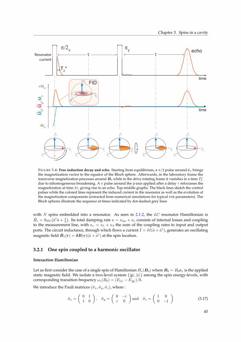
Chapter 3. Spins in a cavity
π/2x πyτ τ
ez
ey
ex~
~
ez
ey
ex~
~
ez
eyex~
~
echo
ez
ey
ex~
~~
ez
ey
ex
~
ez
ey
ex
+Mth
-Mth
Mx, M
y, Mz
Resonatorcurrent
~
~
FID
T2*
time
time
FIGURE 3.4: Free induction decay and echo. Starting from equilibrium, a π/2 pulse around ex bringsthe magnetization vector to the equator of the Bloch sphere. Afterwards, in the laboratory frame thetransverse magnetization precesses aroundB0 while in the drive rotating frame it vanishes in a time T ∗
2
due to inhomogeneous broadening. A π pulse around the y-axis applied after a delay τ refocusses themagnetization at time 2τ , giving rise to an echo. Top-middle graphs: The black lines sketch the controlpulses while the colored lines represent the induced current in the resonator as well as the evolution ofthe magnetization components (extracted from numerical simulations for typical ESR parameters). TheBloch spheres illustrate the sequence at times indicated by dot-dashed grey lines
with N spins embedded into a resonator. As seen in 2.1.2, the LC resonator Hamiltonian isHc = ~ω0
(a†a+ 1
2
). Its total damping rate κ = κint + κc consists of internal losses and coupling
to the measurement line, with κc = κ1 + κ2 the sum of the coupling rates to input and outputports. The circuit inductance, through which flows a current I = δI(a+ a†), generates an oscillatingmagnetic field B1(r) = δB(r)(a+ a†) at the spin location.
3.2.1 One spin coupled to a harmonic oscillator
Interaction Hamiltonian
Let us first consider the case of a single spin of Hamiltonian Hs(B0) whereB0 = B0ez is the appliedstatic magnetic field. We isolate a two-level system |g〉, |e〉 among the spin energy-levels, withcorresponding transition frequency ωs(B0) = (E|e〉 − E|g〉)/~.
We introduce the Pauli matrices (σx, σy, σz), where :
σx =
(0 11 0
), σy =
(0 −ii 0
)and σz =
(1 00 −1
)(3.17)
45

Chapter 3. Spins in a cavity
B0
κ1 spins κ2
ω0
βa
g
FIGURE 3.5: The interaction between spins and resonator is described quantum-mechanically by aspin-photon constant noted g, which is the product of the spin magnetic dipole moment and the magneticfield vacuum fluctuations at the spin location.
One can also define σ± = 12 (σx ± iσy), whose matrix forms are:
σ+ =
(0 10 0
)and σ− =
(0 01 0
)(3.18)
In the basis |e〉, |g〉, the spin Hamiltonian reduces to:
Hs(B0) =~ωs(B0)
2σz, (3.19)
The magnetic coupling of the spin to the resonator is described by the interaction Hamiltonian:
Hint = −~γeS · B1 = −~γeδB(r) · S(a+ a†) (3.20)
In the spin-basis restricted to |e〉, |g〉, H(eg)int =
∑i,j=e,g〈i
∣∣∣| Hint | j〉 |i〉〈j| ⊗ 1c , so that:
H(eg)int = ~(a+ a†)[gσ+ + g∗σ− + Diag(αe, αg)]
with:g = −γe〈e | δB(r) · S | g〉 (3.21)
and αe = −γe〈e | δB(r) · S|g〉 and similarly for αg. The above expression can be simplified furtherby the following procedure (see [62]). The eigenstates |e〉 and |g〉 are first redefined so as to haveg = g∗. Then, if the time-dependent Hamiltonian H
(eg)int is treated as a perturbation of the static
Hamiltonian H0 = Hc + Hs, its expression in the interaction picture is Hint = U0H(eg)int U†0 , where
U0 = exp(iH0t/~) is the interaction evolution operator. By expanding U0 in series, Hint develops in:
Hint(t) = g[σ+aei(ωs−ω0)t + σ+a
†ei(ωs+ω0)t (3.22)+σ−ae
−i(ωs+ω0)t + σ−a†e−i(ωs−ω0)t] (3.23)
+Diag(αe, αg)[aeiω0t + a†e−iω0t] (3.24)
Hint(t) =RWA
g[σ+aei(ωs−ω0)t + σ−a
†e−i(ωs−ω0)t] (3.25)
where we have applied the rotating wave approximation (RWA) to neglect terms in ±(ωs + ω0) be-cause they rotate much faster than those having frequency ±(ωs−ω0). Reverting to the Schrödingerpicture yields the well-known Jaynes-Cummings Hamiltonian [63]:
H(eg)int = ~g(σ+a+ σ−a
†) (3.26)
The two remaining terms in the Hamiltonian describe respectively the absorption of a photon by the
46

Chapter 3. Spins in a cavity
100 150 200
1
0.5
0
Pe(t)
Time t/4g
κ=50 gκ=g/5
T1 = 4g2/κ
FIGURE 3.6: Weak and strong regime for a single-spin. The population of state |e, 0〉, obtained by solv-ing Eqs. 3.30-3.33, presents oscillations when in the strong coupling regime (g > κ) and an exponentialdecay of characteristic rate 4g2/κ in the weak coupling regime.
spin, and its emission; those are the basic processes on which the whole field of CQED is built. Oneprominent phenomenon predicted by the Jaynes-Cummings Hamiltonian is that a spin placed in theexcited state can emit and re-absorb reversibly a single photon into an empty cavity at a frequencyg; this phenomenon is known as vacuum Rabi oscillations [39].
If the system were perfectly isolated from any environment, these oscillations could last indefinitely.However several mechanisms limit the duration of these coherent exchanges: the resonator has adamping rate κ, giving the characteristic lifetime for an intra-resonator photon of 1/κ and the spinlooses its coherence at a rate γ = 1/T2, as described in 3.1. Thus one distinguishes two regimes:
• Strong coupling regime when g κ, γ: the excitations in the system are long-lived comparedto the Rabi period and one may observe Rabi oscillations [39], as shown in Fig. 3.6.
• Weak coupling regime when g κ, γ: excitations decay faster than the coherent evolutionbetween spin and the cavity, thus Rabi oscillations are suppressed.
For an electronic spin-1/2 with γe/2π = 28 GHz/T located d = 10 µm away from a wire-likeinductance embedded in a resonator of frequency ω0/2π = 7 GHz and impedance Z0 = 50 Ω, g canbe estimated to:
g = γe|〈e | δB(r) · S|g〉| = γe2|δB⊥(r)| ≈ γe
2
µ0δi
2πd=γe2
µ0ω0
2πd
√~
2Z0⇒ g/2π ≈ 13Hz (3.27)
This is much smaller than the damping rates of typical ESR resonant circuits, so that ESR experimentsare in the weak coupling regime. In the following, we will see that even in the weak coupling regime,the quantum treatment of the spin-cavity interaction and of field relaxation via a transmission line(see 2.1.3) yields interesting new effects.
Dynamics of the spin-cavity system coupled to a bath
In an ESR experiment, the spin-cavity system is driven and probed via a transmission line coupledwith rate κ1 to the cavity mode. Assuming a coherent state drive sent on port 1, as shown in Fig. 3.5,the drive Hamiltonian is Hd/~ = i
√κ1(βa†e−iωdt + β∗aeiωdt), where β is the amplitude of the drive
and ωd the drive frequency. The Hamiltonian of the system in the frame rotating at ωd is:
H/~ = ∆0a†a+
∆s
2σz + g(σ+a+ σ−a
†) + i√κ1(βa† − β∗a) (3.28)
47

Chapter 3. Spins in a cavity
where ∆0 = ω0 − ωd and ∆s = ωs − ωd. The state of the system |ψ〉 at time t is described by a matrixdensity ρ(t). The system evolution can be described by a Lindblad equation written using ρ as:
ρ = − i~
[H, ρ] +∑
α
Lα[ρ] (3.29)
where Lα[ρ] are called superoperators and are defined as LαρL†α − 12L†αLα, ρ. Each superoperator
is used to describe an interaction with the environment. The cavity leakage due to coupling tothe measurement lines or to internal losses is described by Lr =
√κa. Spin energy relaxation is
described by L1 =√
Γ1σ− and spin decoherence by L2 =√γ/2σz [64].
Eq. 3.29 fully characterizes the evolution of the system. It is valid both in the strong and weakcoupling regimes. In the latter however, it can be simplified to retrieve the classical Bloch equations,supplemented by an additional effect of quantum origin : spin relaxation by the Purcell effect.
Purcell effect
To evidence cavity-enhanced spin relaxation by the Purcell effect, we now present a simple argumentfound in [39]. Consider the undriven spin-cavity system, with the spin prepared at time t = 0 inthe excited state |e〉 and no photon in the cavity, and at zero temperature. The system evolutioncan be written using only the basis composed of |g, 0〉, |g, 1〉 and |e, 0〉 states. Using Eq. 3.29 with∆ = ∆0 − ∆s and ∆s = 0 (and neglecting non-radiative spin decoherence processes, i.e. takingΓ1 = γ = 0) yields the following equations for the spin-cavity density matrix ρ:
ρe0,e0 = −ig(ρe0,g1 − ρg1,e0) (3.30)ρg1,g1 = −κρg1,g1 + ig(ρe0,g1 − ρg1,e0) (3.31)
ρe0,g1 = −(κ
2+ i∆
)ρe0,g1 − ig(ρe0,e0 − ρg1,g1) (3.32)
ρ = −(κ
2− i∆
)ρg1,e0 + ig(ρe0,e0 − ρg1,g1) (3.33)
In the weak-coupling regime g κ, the probability ρg1,g1 of finding a photon in the cavity decaysmuch faster than the rate at which the spin can transfer its excitation via Rabi oscillations. As a resultthe cavity is nearly always empty ρg1,g1 ≈ 0. In this regime, one can also assume that the coherenceterms ρe0,g1 and ρg1,e0 follow adiabatically the variations of the excited state population [39] suchthat ρg1,e0 ≈ 0 and ρe0,g1 ≈ 0. According to these three assumptions, Eqs. 3.32 & 3.33 yield:
ρe0,g1 =−ig
κ/2 + i∆ρe0,e0 (3.34)
ρg1,e0 =ig
κ/2− i∆ρe0,e0 (3.35)
We now replace ρe0,g1 and ρg1,e0 in Eq. 3.30, leading to:
ρe0,e0 = −g2
(1
κ/2 + i∆+
1
κ/2− i∆
)ρe0,e0 (3.36)
We thus obtain that ρe0,e0 is exponentially damped, at the so-called Purcell rate given by:
Γp(∆) =κg2
κ2/4 + ∆2(3.37)
48

Chapter 3. Spins in a cavity
This is illustrated in Fig. 3.6 where we show a numerical integration of Eqs. 3.30-3.33 both in thestrong and in the weak coupling regime. We stress that treating the resonator field quantum-mechanically is essential to derive this Purcell effect, which is a direct manifestation of the action ofquantum fluctuations on the spin dynamics.
Resonator adiabatic elimination
A more rigorous treatment of the Purcell effect in a quantum optics theoretical framework, whichalso takes into account the presence of a drive, relies on adiabatic elimination of the resonator-fieldvariables (see [64, 27, 65, 66] and references within). We summarize here the main results. First, oneseparates the field operator from its mean value by writing:
a = α+ c, with 〈c〉 = 0 (3.38)
In the absence of the spin, the steady-state value of α is given by the input-output relations (seeEq. 2.52): α = 2
√κ1β/(κ + 2i∆0). In the limit g κ, the adiabatic elimination of the resonator
operators c and c† then yields the following master equation in the drive rotating frame [65] for thereduced spin density matrix ρ:
ρ = −i[Heff , ρ] + L1[ρ] + L2[ρ] + Lp[ρ], (3.39)
with the effective Hamiltonian Heff being [64]:
Heff/~ =∆s − ξ
2σz + g(ασ+ + α∗σ−) (3.40)
where ξ = ∆g2
∆2+κ2/4 . The extra ξ term renormalizes slightly the spin frequency. As the correction isonly of order g2/κ, we neglect it in the following.
In addition to modifying Heff , the adiabatic elimination of the resonator operator is responsible forthe appearance of a new spin superoperator Lp =
√Γp(∆)σ− where Γp is the decay rate given in
Eq. 3.37 [64]. This novel relaxation channel is precisely the cavity-enhanced spontaneous emission,i.e. the Purcell effect.
Within this approximation, the semi-classical equations of motion for the spin observables and theintra-cavity field in the drive rotating frame can be derived from Eqs. 3.38-3.39. For the sake ofsimplicity, we consider here that α is a real number; we write ω1 = −2gα so that:
d
dt〈σx〉 = ∆s〈σy〉 − γ⊥〈σx〉 (3.41)
d
dt〈σy〉 = −∆s〈σx〉 − ω1〈σz〉 − γ⊥〈σy〉 (3.42)
d
dt〈σz〉 = ω1〈σy〉 − [Γ1 + Γp(∆)](〈σz〉+ 1) (3.43)
〈a〉 = α− i2g
κ+ 2i∆〈σ−〉 (3.44)
with γ⊥ = γ + Γ1
2 +Γp2 . Eqs. 3.41-3.43 are thus identical to the Bloch equations (see Eqs. 3.9-3.10)
with only in addition a new T1 relaxation channel given by the Purcell effect.
Note that in presence of a finite photon thermal population in the resonator nth the Lindbladoperator Lp is changed into the sum of Lp+ =
√Γpnthσ+ and Lp− =
√Γp(nth + 1)σ−, which
describes spontaneous and stimulated emission as well as absorption. If no other relaxation process
49

Chapter 3. Spins in a cavity
is present (Γ1 = 0), Eq. 3.43 is modified into [27]:
d
dt〈σz〉 = ω1〈σy〉 − (2nth + 1)Γp(∆)
[〈σz〉+
1
2nth + 1
](3.45)
This implies that the relaxation is enhanced by a factor (2nth + 1) while the polarization is decreasedby the same factor.
In addition to showing cavity-enhanced spin-relaxation, Eqs. 3.41-3.43 also provide a way to computethe signal emitted from the spin. We see that the intra-cavity field is changed by 2ig/(κ+ 2i∆)〈σ−〉in the presence of the spin; the output signal leaking from the cavity is readily computed thanks toinput-output theory as 〈aout〉 =
√κ〈a〉 (see Eq.2.50). We thus come to the conclusion that the spin
emits a microwave signal in the detection waveguide that is roughly given by 〈aout〉 = 2g〈σ−〉/√κ
at resonance (∆ = 0). This equation is the quantum-optics analog of the classical inductive detectiondescribed in 3.1.3. The output signal is proportional to the spin transverse magnetization, to thespin-photon coupling constant, and to 1/
√κ.
3.2.2 Collective effects
We have seen up to now that a spin weakly coupled to a resonator is well described by the classicalBloch equations, with an extra relaxation channel given by the Purcell spontaneous emission rate.In the following we discuss the validity of this description for an ensemble of spins.
N identical spins model
We consider first the ideal case of N identical spins-1/2 with frequency ωs coupled with samecoupling constant g to the resonator. The system Hamiltonian is the sum of the Jaynes-CummingsHamiltonians associated with each spin, and is known as the Tavis-Cummings Hamiltonian [67]:
HTC/~ = ω0(a†a) +ωs2
N∑
j=1
σ(j)z + g
N∑
j=1
(σ(j)+ a+ σ
(j)− a†) (3.46)
where (j) refers to the operators of spin j. This Hamiltonian acts on Es ⊗ Ec, where Es is the 2N -dimensional Hilbert state spanned by the states |ε1, . . . , εn〉, εi = gi, ei and Ec is the resonatorHilbert space. Introducing the collective spin operators Sk =
∑Nj=1 σ
(j)k , the Hamiltonian can be
rewritten as:HTC/~ = ω0(a†a) +
ωs2Sz + g(S+a+ S−a†) (3.47)
A remarkable property of this Hamiltonian is that the total spin angular momentum S2
= S2x + S2
y +
S2z is conserved in time since [HTC, S
2] = 0. It is therefore interesting to introduce the basis |S,m〉
of joint eigenstates of S2
and Sz , defined as:
S2|S,m〉 = S(S + 1)|S,m〉 (3.48)Sz|S,m〉 = m|S,m〉. (3.49)
S can take any positive values among N/2, N/2 − 1, ...; and m can take any values among−S,−S + 1, ..., S − 1, S. Since S is conserved in time, the system dynamics is restricted to stateshaving the same S as the initial state. Within one S subspace, m + S describes the number ofexcitations that can be exchanged with the resonator. For instance, emission of a photon takesthe system from |S,m〉 ⊗ |0〉 to |S,m− 1〉 ⊗ |1〉. Photon absorption or emission is thus impossiblefor all states for which S = 0, meaning that they are strictly dark states. For other states, the
50

Chapter 3. Spins in a cavity
κ
ω0
S=N/2
m=N/2
m=N/2-1
m=N/2-2
m=-N/2
m=-N/2+1
m=-N/2+2
S=N/2-1
...
S=N/2-2N-1 degenerate N(N-3)/2 degenerate
N√
g
〉E|
〉B|
〉G|trapped states
γ
Γp(S+m)(S-m+1)
FIGURE 3.7: N identical spins. For a system of N identical spins, the system dynamics are confined tofixed S manifolds, creating state-dependent coupling to the resonator and inducing non-exponentialrelaxation most often towards trapped states.
coupling is dependent of (S,m) and is maximal for states within the S = N2 manifold. In particular
this manifold comprises the ground state |G〉 = |g1, . . . , gn〉 and the one-excitation state |B〉 =1√N
∑j |g1, . . . , ej , . . . , gn〉. One can observe that:
〈B, 0∣∣∣HTC|G, 1〉 = ~g
√N (3.50)
thus |B〉 and |G〉 can exchange one excitation with the resonator at an enhanced rate g√N . This
collective enhancement of the vacuum Rabi oscillations has been observed first for atoms [68], andmore recently with superconducting qubits [69] and spins [70]. By considering |B〉 and |G〉 as atwo-level-system, it led to the implementation of quantum memories with ensemble of spins [71].The state of another qubit, such as a superconducting qubit, can be transferred to the ensemble so asto be stored and thus benefit from the spin ensemble longer coherence time.
Another direct consequence of this model is the deep modification of the radiative properties ofan ensemble of identical spins compared to the single spin spontaneous emission case ([72], seeFig. 3.7). Not only can |S,m〉 only relax towards |S,m − 1〉 but the emission takes place at a rateΓp(S +m)(S −m+ 1) which depends very strongly on S and m. For instance, if the spin ensembleinitially starts from the fully excited state |E〉 = |e1, . . . , en〉 which corresponds to
∣∣N2 ,
N2
⟩, it will
desexcite itself within the S = N2 manifold. As the transition probabilities are not constant (i.e.
for higher m the transition probabilities start as ∝ m but reach a maximum ∝ S2 when m goesthrough zero before decreasing again), the relaxation towards state |G〉 is not a simple exponentialof rate Γp, but a much faster super-radiant pulse whose shape and properties have been studied indetail [72, 73], and which corresponds to the operation of a maser in pulsed mode [74].
For other initial states comprised in manifolds S 6= N2 , the excitation is also non-exponential and
strongly dependent on S : the |E〉 state has a super-radiant relaxation, much faster than Γp, whereasstates S = 0 do not relax radiatively at all. More importantly, the ground state |G〉 cannot bereached any longer for any initial state within manifolds S 6= N
2 . They can only relax down to thelowest-energy states of their S manifold, which have the form |S,−S〉, and which in general still
51

Chapter 3. Spins in a cavity
0 1 2 3 4
−2
0
2
4
6
time (s)0 1 2 3 4
0
2
4
6
time (s)
a b
〉z
S 〈
〉z
S〈
∆ ∆
FIGURE 3.8: Spin relaxation simulated for 5 spins starting from a disordered state. Black: ideal exponen-tial Purcell relaxation (Γp = 1 s−1), blue 〈Sz〉. a Without inhomogeneous broadening, the relaxation goesto a trap state b whereas for sufficiently large inhomogeneous broadening (spins spaced by 1 Hz), a fullyexponential decay is observed. Adapted from [27].
contain many spins in their excited state. One can say that the system becomes trapped in thesehighly correlated states, instead of relaxing to its true ground state |G〉.Summing up, we see that the radiative relaxation of an ensemble of identical spins seems to becompletely different from the single-spin case, where an exponential relaxation of rate Γp is predicted.Since relaxation now depends on the initial state of the ensemble, and is in general not exponential,a description by the Bloch equations with a single relaxation time T1 seems clearly impossible.
Collective or individual relaxation ?
The conclusions reached above on the radiative properties of an ensemble of identical spins heavilyrely on symmetry properties of the system Hamiltonian. It should thus not come as a surprisethat these conclusions are strongly altered when one takes into account two phenomena : spindecoherence, and inhomogeneous broadening of the spin linewidth, both of them characterized bya finite ensemble spin linewidth γ.
The rigorous treatment of the effects of inhomogeneous broadening and decoherence on the radiativeproperties of a spin ensemble is a difficult theoretical problem, which has been addressed in a fewarticles [75, 27, 76]. The outcome of all these works is that in the limit of strong decoherenceor inhomogeneous broadening, collective radiative effects are suppressed, and one recovers thesituation of a collection of spins radiating independently at a rate Γp. As a result, the spin ensemblecan now truly relax to its ensemble ground state (at rate Γp), and trapping in correlated states doesnot occur any longer. To discriminate between the "independent" or "collective" radiative regime,one has to consider a dimensionless parameter called the ensemble cooperativity defined as:
C =2Ng2
κγ(3.51)
Collective effects are found in the so-called strong collective coupling regime C 1; independentradiation from each spin at rate Γp is obtained in the so-called weak collective coupling regimeC 1. In the remaining of this thesis, we will be in the latter regime.
52

Chapter 3. Spins in a cavity
A clear manifestation of these two situations is seen in Fig. 3.8, which is extracted from [27]. Acollection of 5 spins 1/2 is considered, starting at t = 0 from a fully unpolarized state. When all spinshave the same frequency, the spins relax towards a partially polarized state for which 〈Sz〉 ≈ 2.8,much less than the true ground state for which 〈Sz〉 = 5. When some frequency inhomogeneity istaken into account, the ensemble relaxes towards the true ground state, at a rate exactly given bythe single-spin Purcell rate, Γp.
Dynamics of the system
In the following, we will often need to simulate the dynamics of an ensemble of N spins whencoupled to the cavity. To treat numerically this problem, our collaborator Brian Julsgaard fromAarhus University has written a code [77, 78] that we will use, based on the equations that arepresented in the following. Consider a spin ensemble with an inhomogeneous linewidth andnon-identical coupling strengths. The spin ensemble is divided intoM sub-ensembles regardedeach as homogeneous with coupling strength gm, spin resonance frequency ωd + ∆m and containingNm spins for m = 1, . . . ,M [77]. For each sub-ensemble, collective spin observables S(m)
k can beintroduced. The Hamiltonian of Eq. 3.46 expressed in the rotating frame in presence of a drive istransformed into:
HTC/~ = ∆0(a†a) +M∑
m=1
∆m
2S(j)k +
M∑
m=1
gm(S(m)+ a+ S(m)
− a†) + i√κ1(βa† − β∗a) (3.52)
Rewriting the master equation of Eq. 3.29 for these collective variables and assuming identical T1
and T2 processes for each sub-ensemble allows to derive the following equations for the mean-valueof each operator:
d
dt〈a〉 =
√κ1β − i∆0〈a〉 −
κ
2〈a〉 − i
M∑
j=1
gm〈S(m)− 〉 (3.53)
d
dt〈a†〉 =
√κ1β
∗ + i∆0〈a†〉 −κ
2〈a†〉+ i
M∑
j=1
gm〈S(m)+ 〉 (3.54)
d
dt〈S(m)x 〉 = −∆s〈S(m)
y 〉 −√
2gm〈S(m)z 〉〈Y 〉 − γ⊥〈S(m)
x 〉 (3.55)
d
dt〈S(m)y 〉 = ∆s〈S(m)
x 〉 −√
2gm〈S(m)z 〉〈X〉 − γ⊥〈S(m)
y 〉 (3.56)
d
dt〈S(m)z 〉 =
√2gm〈Y 〉〈S(m)
x 〉+√
2gm〈X〉〈S(m)y 〉 − Γ1(〈S(m)
z 〉 −Nm) (3.57)
where X and Y are the intra-resonator quadrature operators. This set of equations can be used tocompute numerically the evolution of the mean values for each sub-ensemble. To solve the completebehavior of the system, spin ensemble and resonator, one needs to solve 3M + 2 differentialequations, three for each sub-ensemble and two for the resonator. Provided that M is not toolarge, this can be done numerically. We use this approach in ch. 7 to simulate a complete spin-echosequence in our experiment.
53

Chapter 4
Bismuth donors in silicon
In this third and last background part, we describe the spin system that we use throughout thisthesis: bismuth donors in silicon (Si:Bi). Group V donors in silicon were studied as early as 1954,with pioneering works from Honig and Feher [79, 80] focusing extensively on phosphorus andarsenic. The very long values reported for T1 (> 1000 s [81]) and T2 = 0.2 ms for Si:P lead alreadyin these early days to the idea of using the spin to store classical information [82]. Later on, Kaneextended this suggestion to building a quantum computer based on Si:P [83], triggering a renewedintense interest in these systems, seen as "spins living in a semiconducting vacuum”.
Indeed, in the quest for ideal qubit candidates, the thoroughly-studied silicon appears, alongwith carbon, as a promising host material since its main isotope 28Si has zero nuclear spin so thatan enriched 28Si sample would provide a magnetically-silent environment for donor spins. Theelectronic spin 1/2 of a donor in silicon is seen as a particularly promising qubit candidate dueto its long-lived coherence and fast manipulation time. Bismuth 209Bi is the heaviest group Vdonor in silicon (see Table 4.1); other donors include 31P, 33As, 121,123Sb. In early studies, bismuthgathered less attention than phosphorus due to the latter simplicity and use in modern CMOS devices.However, bismuth received renewed attention recently due to the existence of optimal workingpoints, where the Si:Bi frequency becomes insensitive to magnetic field fluctuations [84] leadingto the longest measured coherence times for electronic spins in the solid state [25]. In addition, itslarge zero-field splitting makes it attractive for coupling to superconducting resonators which couldbe useful for building a quantum memory for superconducting qubit states [85].
Donor 31P 33As 121Sb 121Sb 209BiED (meV) 45.6 53.8 42.8 42.8 71.0a0 (nm) 16.8 15.5 17.3 17.3 11.5∆E (meV) 13.0 22.5 12.3 12.3 41I 1/2 3/2 5/2 7/2 9/2A (MHz) 118 198 186 101 1475.4
TABLE 4.1: Group V donors characteristics: ionization energy (ED), apparent Bohr radius (a0), nuclearspin and hyperfine coupling constant (A). Extracted from [16, 86, 87, 88].
This chapter will present the essential information to understand the experimental work presentedin this thesis. When available we indicate references the reader may consult for more detailedderivations and explanations. In what follows, we briefly present the electronic structure of Si:Bi(see [89]) before describing its spin Hamiltonian, energy levels and ESR transitions (see the workof Mohammady et al. [84]). We list the known relaxation mechanisms (see [81, 90]) as well as theexpected sources of decoherence (see [91]). Last we present the characteristics of the sample used inour experiments.
54

Chapter 4. Bismuth donors in silicon
X
Ene
rgy
(eV
)
5
0 gap
k-pointΓ L X
Ec
209Bi
kx
kz
ky
Γ
X
L
0.54 nm
a b c
FIGURE 4.1: An atom in silicon. a Silicon diamond lattice with a single substitutional bismuth impurity.b Band diagram of silicon. c First Brillouin Zone, with the six-valley of the conduction band highlightedin yellow. Blue ellipsoids symbolize iso-energy surfaces. The Γ-point, center of the valence band isindicated in red.
4.1 A substitutional donor in silicon
Silicon is a group IV semi-conductor which crystallizes in a diamond structure (see Fig. 4.1a). EachSi atom forms a covalent bond with the four neighboring atoms in a tetrahedron geometry. Theassociated Brillouin zone is shown in Fig. 4.1c. The calculation of the band structure of siliconreveals it has an indirect band-gap Eg = 1.1eV at T = 300 K (see Fig. 4.1b). The conduction band issix-fold degenerate with each minimum offset from the maximum of the valence band occurringat the center of the first Brillouin Zone (Γ point) by ±0.85 2π/a along the vectors ±kx, ±ky , ±kz , abeing the lattice parameter (0.543 nm for silicon) as shown in Fig. 4.1c. Each minimum is referred toas a silicon valley.
Bismuth donors are substitutional impurities in silicon. A Bi atom replaces a Si atom and fourof its valence electrons form covalent bonds with the electrons of the neighboring Si atoms (seeFig. 4.1a). The fifth electron can be either ionized into the conduction band (state D+) or bound tothe Bi nucleus forming a “neutral donor” (state D0). The energy required to ionize the donor to theconduction band is ED = −71 meV [88].
4.1.1 Electronic states
As ED Eg, Si:Bi are shallow impurities. In this case, the donor wavefunction can be expressedusing combinations of the crystal Bloch wave functions using the framework of effective masstheory (EMT) (developed by Kohn and Luttinger [92], see also [93]). The attractive potential V(r)of the Bi nucleus is modeled as a Coulomb potential with V (r) = −e2/(εSir), where εSi is thesilicon dielectric constant. As it extends over many lattice sites, the donor electronic wavefunctionis only weakly confined (see Fig. 4.2a). EMT predicts a six-fold degenerate 1s ground state withequivalent wavefunctions expressed as a product of the conduction-band Bloch functions φkµ(r)and an hydrogen-like envelope function Fµ(r) at the µ-th conduction-band valley [94]:
Ψ(r) =∑
µ
αµFµ(r)φkµ(r) (4.1)
The spatial extension of the hydrogenic envelope Fµ(r) is given by a parameter a0 called the Bohrradius, shown in Table 4.1. The coefficients |αµ|2 give the probability of finding the donor electron
55

Chapter 4. Bismuth donors in silicon
|Ψ(r)|
V(r)
a b
Bi+
Conduction BandEc
Kohn-Luttinger(EMT)
1s(6)E(2)T2(3)
A1(1)
valley-orbitsplitting
alattice parameter
ED
FIGURE 4.2: Bismuth electronic states. a Illustrative schematic of the donor wave function and of theCoulomb potential compared to the lattice parameter. b Six-fold degenerate ground states predicted byeffective mass theory and with an additional valley-orbit interaction perturbation.
in the µ-th valley and are called valley population. In this simplistic picture, EMT produces identicalresults for all of the donors, with calculations indicating identical Bohr radii and ED = −31.3 meV.
This is in direct contradiction with the experimental results where instead of a single degeneratestate three distinct energy-levels are observed [87]. The discrepancy is explained by a break downof the EMT approach in the vicinity of the donor nucleus. To correct this effect and take into accountthe tetrahedral environment surrounding the donor in the central cell as well as the core andvalence electrons screening the Bi nucleus attractive potential, a phenomenological interaction called“valley-orbit” is added as a perturbation of EMT [94]. With this improved model, the degeneracyof the ground state is lifted, yielding three distinct 1s states labeled by their tetrahedral symmetrygroup designation : a symmetrical ground-state A1, a three-fold degenerate level T2 and a two-folddegenerate level E. The corresponding eigenstates may be written in the same manner as in Eq 4.1with envelope hydrogenic functions (see Fig. 4.1.1a). Written in the valley basis ±kx,±ky, ±kz,the states are:
A1 = 1√61, 1, 1, 1, 1, 1 T2z =
1√20, 0, 0, 0, 1,−1 (4.2)
T2x = 1√21,−1, 0, 0, 0, 0 Exy =
1
21, 1,−1,−1, 0, 0 (4.3)
T2y = 1√20, 0, 1,−1, 0, 0 Ez =
1√12−1,−1,−1,−1, 2, 2 (4.4)
This treatment yields different ionization energies and Bohr radii for the five silicon donors, inagreement with measurements (see Table 4.1). Bismuth is the deepest donor, and its wavefunctionsare correspondingly more confined with a smaller Bohr radius. In the remaining part of this chapter,we are mainly interested in the spin properties of the neutral Bismuth donor in its ground state A1,but the properties of higher-energy states do play a role in the donors physics, as will be clear later.
Charge state
The charge state of the bismuth donors in silicon is found by calculating the position of the Fermi-level as a function of temperature, see Neamen [95]. At zero temperature, for a n-type semiconductor,all donors retain their electrons and thus the Fermi level energy will be situated mid-way throughthe donor energy level A1 (see below) and the conduction band : EF = 1
2 (EC − EA1). At slightly
higher temperature, the donors electrons start being excited to the conduction band and the fractionof ionized donors is given by:
N+D
ND=
1
1 + 2e(EF−EA1)/kBT
(4.5)
56

Chapter 4. Bismuth donors in silicon
1
0 0 50 100 150 200Temperature (K)
Frac
tion o
f ioniz
ed do
nors
T=0 K T<400 K
a b
EC
EA1
EF
conduction band
Fermi level
FIGURE 4.3: Charge state of a bismuth donor. a At non-zero temperature, electrons bound to donorsare excited to the conduction band, resulting in a partial ionization of the donors and a lowering of theFermi energy level. b Fraction of ionized donors N+
D/ND as a function of temperature in the case ofbismuth, evaluated with ED = 71 meV and ND = 1016cm−3.
where ND is the total concentration of donors and N+D is the concentration of ionized donors. Since
the silicon gap is much larger than the ionization energy of the shallow donors, for low enoughtemperatures (T < 400 K) the valence electrons can not be excited to the conduction band and thusthe concentration of free carriers in the conduction band n is only given by the concentration ofionized donors: n = N+
D . The concentration of free carriers is also linked in case of non-degeneratesemi-conductors to the temperature by:
n = Nce(EF−EC)/kBT , (4.6)
where Nc = 2(2πm∗kBT/h2)3/2 is the effective density of states in the conduction band with m∗
being the effective mass of an electron. Thanks to these two relations, Eq 4.5 may be rewritten to de-termine n as a function of the temperature T , the donor ionization energy ED and the concentrationof donors:
n =ND
1 + 2n/Nξ(4.7)
where Nξ = Nce−ED/kBT .
As the electrons are moving from the donor level to the conduction band as a function of temperature,the Fermi energy tends to move downwards. Precise determination of the Fermi energy as a functionof n is given by Eq 4.6. One can then access the fraction of ionized donors by evaluating Eq 4.5. Withan ionization energy ED = 71 meV and for a concentration ND = 1016cm−3, bismuth donors are intheir neutral state up to T = 40 K, see Fig. 4.3b. In our experiments which take place at millikelvinstemperatures, all donors should be in their neutral state. However, note that other factors mayimpact the charge states of donors, such as internal electric fields [96, 97] or bending of the energylevels in presence of Schottky barriers; we will come back to this issue later in ch. 7.
57

Chapter 4. Bismuth donors in silicon
0.2 0.4 0.6
-10
-5
0
5
10
B0(T)
Ene
rgy
(GH
z)
mS=1/2, mI=9/2
mS=1/2, mI=-9/2
mS=-1/2, m
I=-9/2
mS=-1/2, m
I=9/2
9A/4
-11A/4
+, m=5
-, m=4
+, m=-5
-, m=-4
1 2 3 45678910
111213
20 19 18 17161514
FIGURE 4.4: Bismuth energy spectrum. Energy-levels computed from the diagonalisation of the Si:BiHamiltonian as a function of B0 (Eq 4.8). The coupled energy-levels E
±m are color-coded from purple to
red, the uncoupled energy-levels are in black. Figure adapted from [99, 84].
4.2 Spin levels and ESR-allowed transitions.
A neutral bismuth donor in silicon has spin properties arising from the coupling of the S = 1/2electronic spin to the 209Bi I = 9/2 nuclear spin. When placed in an external magnetic fieldB, itstwenty energy levels are described by the following spin Hamiltonian that includes a Zeeman effectfor electronic and nuclear spin and an isotropic hyperfine coupling [98]:
H/~ = B ·(γeS ⊗ 1− γn1⊗ S
)+AS · I (4.8)
where γe/2π = 27.997 GHz/T and γn/2π = 6.962 MHz/T are the electronic and nuclear gyromag-netic ratio and A/2π = 1.4754 GHz is the hyperfine coupling constant [26]. To understand thissystem, we will follow the analysis made by Mohammady at al. in [84]. Assuming a static magneticfield directed along z,B0 = B0ez , the Hamiltonian may be re-written as:
H0/~ = ASz Iz +A
2(S+I− + S−I+) + ω0(Sz − δIz) (4.9)
where ω0 = B0γe and δ = γn/γe ≈ 10−3. Due to the hyperfine coupling, the Hamiltonian is notdiagonal in the Zeeman basis spanned by |ms,mi〉 with ms = ± 1
2 and mi = −92 . . . 9
2 and itsenergy states are instead hybridized electro-nuclear states. The energy spectrum as a function ofmagnetic field obtained from the Hamiltonian diagonalization is shown in Fig. 4.4.
58

Chapter 4. Bismuth donors in silicon
Hybridized eigenstates
To understand the spectrum in Fig. 4.4 and the spin properties of the eigenstates, one can noticefirst that the projection m = mi + ms of the total angular momentum operator F = I + S ontoez is a good quantum number since [H, Sz + Iz] = 0. If we then consider the application of theHamiltonian on a state of the Zeeman basis:
H0/~|±1
2,mi〉 =
(±A
2mi ±
ω0
2+ ω0δmi
)|±1
2,mi〉+
A
2I±|∓
1
2,mi〉 (4.10)
it appears that | 12 , 92 〉 and |− 1
2 ,− 92 〉 are unmixed eigenstates of the Hamiltonian since I±|∓ 1
2 ,± 92 〉 = 0.
Their energies are:
E|± 12 ,± 9
2 〉 =9
4A± ω0
2(1 + 9δ) (4.11)
These states are the only ones in the spectrum (see Fig. 4.4) to have a linear energy dependence onB0. When |m| < 5, |± 1
2 ,mi〉 hybridizes with |∓ 12 ,mi±1〉. From these observations, the Hamiltonian
expressed in the Zeeman basis can be decomposed into two one-dimensional Hamiltonians actingon bases
|12,
9
2〉and|−1
2,−9
2〉 (4.12)
and nine two-dimensional Hamiltonians acting on subspaces labeled by m:
|±1
2,mi〉, |∓
1
2,mi ± 1〉 = |±1
2,m∓ 1
2〉, |m| 6 4 (4.13)
As explained in [84], the restriction of H0 to one of these two-dimensional bases is:
Hm/~ =A
2Rm[cos θmσz + sin θmσx]− A
2ε1 (4.14)
where:
R2m =
[m+
ω0
A(1 + δ)
]2+ (25−m2) (4.15)
tan θm =(25−m2)
1/2
m+ ω0
A (1 + δ)(4.16)
ε =1
2+ 2ω0δm (4.17)
Since cos θmσz + sin θmσx = σ0θm , where σ0θm is the Pauli spin matrix in the rotated basis, theeigen-energies are given by:
E±
m =A
2(−ε±Rm) (4.18)
This expression is exact for all magnetic fields and for all m and yields the energy spectrum ofFig. 4.4. The corresponding energy eigenstates are:
|±,m〉 = a±m|±1
2,m∓ 1
2〉+ b±m|∓
1
2,m± 1
2〉 (4.19)
where
a±m =1√2
(1 + cos θm)1/2 = cosθm2
and b±m = ± 1√2
sin θm(1 + cos θm)−1/2 = ± sinθm2
(4.20)
From this analysis, it appears that the eigenstates can be labeled in multiple ways: by order of
59

Chapter 4. Bismuth donors in silicon
increasing energy |i〉, i = 1, . . . .20, by the coupled basis |±,m〉 and in the high-field limit by theZeeman basis |ms,mi〉,ms = ± 1
2 ,mi = −92 . . . 9
2, see Fig. 4.4. The correspondence between theZeeman basis and the coupled basis is realized by noticing that in the high-field limit, tan θm → 0
(Eq 4.17). Thus a±
m → 1 and b±
m → 0, meaning that the electro-nuclear eigenstates |±,m〉 convergerespectively to the Zeeman eigenstates |ms = ± 1
2 ,mi = m ∓ 12 〉 as expected when the hyperfine
term can be neglected with respect to the Zeeman terms.
Eigen-energies at low magnetic field
The following simplified expressions are readily obtained in the “low-field limit” ω0 = B0γe A,which will be the one relevant for our experiments:
E+m = +
9
4A+
m
10ω0(1 + δ ∓ 10δ)B0 with m ∈ −5, ..5 (4.21)
E−m = −11
4A− m
10ω0(1 + δ ∓ 10δ)B0 with m ∈ −4, ..4 (4.22)
The field B0 is seen to lift linearly the nine-fold and eleven-fold degeneracy of the ground andexcited multiplet (see Fig. 4.4). Transitions from the ground to the excited multiplet have frequenciescentered on 5A/2π ≈ 7.37 GHz. In this low-field limit, the coefficients a
±
m and b±
m describing themixing of the eigenstates are strongly dependent on m.
ESR-allowed transitions
As explained in ch.3 (see Eq. 3.20 and following for instance), spin transitions can be driven if andonly if 〈i|S|j〉 6= 0; in the following, we compute these matrix elements for Si:Bi.
Sx transitions allowed at large magnetic field.
In the high-field limit, the Bismuth donor spin eigenstates are well approximated by the Zeemanbasis and the allowed transitions are thus given by the usual selection rules |∆ms|= 1 and ∆mi = 0.The 10 transitions |ms = 1
2 ,mi〉 ↔ |ms = − 12 ,mi〉 have a matrix element 〈1/2|Sx|−1/2〉 = 1/2, as
expected for an electronic spin 1/2 (see Figs. 4.5 & 4.6b).
Sx transitions allowed at low magnetic field.
At lower magnetic field, states |ms = 12 ,mi〉, |ms = − 1
2 ,mi〉 are progressively hybridized into|+,m〉, |−,m− 1〉 as depicted in Fig. 4.5. Correspondingly, the matrix element of these transitionsbecomes smaller than 1/2 (see Fig. 4.6b). Their matrix elements are:
〈+,m|Sx|−,m− 1〉 =1
2a+ma−m−1 =
1
2cos
θm2
cosθm−1
2
and depend strongly on m at low magnetic field.
In addition to these 10 transitions, transitions between |−,m〉 and |+,m−1〉 become allowed becauseof this hybridization due to the hyperfine interaction. The frequency and matrix-element of theseextra 9 transitions as a function of magnetic field have been plotted in Fig. 4.6c (blue arrows). Theirmatrix elements are:
〈−,m|Sx|+,m− 1〉 =1
2b−mb
+m−1 = −1
2sin
θm2
sinθm−1
2
and go to zero at high field, as expected.
60

Chapter 4. Bismuth donors in silicon
ms = 1/2
ms = -1/2
mi
mi
mi-1
mi-1
mi+1
mi+1
High-field Low-fielda b
+, m+1 +, m +, m-1
-, m-2-, m-1-, m
hyperfinecoupling
FIGURE 4.5: Transitions schematic. a At high-field, the usual ESR transitions between levels |ms =12,mi〉 ↔ |ms = − 1
2,mi〉 are allowed (brown arrows). At lower fields, the hyperfine coupling renders
the Zeeman basis (a) invalid to describe the hybridized electro-nuclear states (symbolized by the blueellipses) however an accurate description is given by the coupled basis |±,m〉 (b). b At low magneticfield, in the coupled basis |±,m〉, the high-field ESR transitions are now labeled |+,m〉 ↔ |−,m − 1〉.The mixing induced by the hyperfine term allows in addition the transitions |−,m〉 ↔ |+,m − 1〉, aswell as |+,m〉 ↔ |+,m− 1〉 and |−,m〉 ↔ |−,m− 1〉.
It is interesting to note that the transitions |+,m〉 ↔ |−,m−1〉 and |+,m−1〉 ↔ |−,m〉 (in the |m 6 4manifold) are quasi-degenerate in frequency and that their matrix elements are complementary:|a+ma−m−1|+|b+m−1b
−m|≈ 1/2. Thus, at any given magnetic field, only 10 transitions have a matrix
element greater than 1/4, see Fig. 4.6b & c (the associated pairs are denoted by a grey circle).
Sz transitions.
An unusual feature of Si:Bi (again, due to the hyperfine coupling) is the existence of 9 transitions thatcan be driven by a microwave fieldB1 parallel to the static fieldB0. These Sz transitions connectlevels |+,m〉 and |−,m〉 in the coupled basis and their matrix element is given by:
〈+,m|Sz|−,m〉 =sin θm
2.
Even if these transitions are forbidden in the high-field limit, they have a sizeable matrix element inthe range [0, 0.4 T] and can thus be observed at low-field. They are shown in pink in Fig. 4.6a, andtheir frequency and intensity dependence on B0 is shown in Fig. 4.6d. It is interesting to note thateach transition comes in-between two Sx transitions.
NMR transitions
In the above description, we have restricted ourselves to transitions whose frequencies lie in thegigaHertz range. In addition, transitions between |±,m〉 and |±,m − 1〉 (with frequencies in theMegaHertz range) are allowed, as shown in grey in Fig. 4.6a. At high fields, these transitions canonly be driven via the nuclear spin matrix element Ix; however at low field they acquire a sizeableSx matrix element:
〈+,m|Sx|+,m− 1〉 =1
2a+mb
+m−1 =
1
2cos
θm2
sinθm−1
2(4.23)
〈−,m|Sx|−,m− 1〉 =1
2a−m−1b
−m = −1
2cos
θm−1
2sin
θm2
(4.24)
These transitions can thus be driven faster than usual nuclear spin transitions, as demonstrated in[85]
61

Chapter 4. Bismuth donors in silicon
high B0
Magnetic field B0 (T) Magnetic field B0 (T) Magnetic field B0 (T)
+, m=5
0
5
10
15
0 0.1 0.2 0.3 0 0.1 0.2 0.3
Freq
uenc
y (G
Hz)
0 0.1 0.2 0.3 0 0.1 0.2 0.3
Sx transitions allowed at high-B0 Sx Transitions forbidden at high-B0
+, m -, m-1
5A
a
cb
0 0.1 0.2 0.3
Mat. El0 0.5
0.1 0.2 0.3
Sz transitions
d
-, m=4
+, m=-5
-, m=-4
+, 4 +, 3 +, 2 +, 1 +, 0 +,-1 +,-2 +,-3 +,-4
-, 3 -, 2 -, 1 -, 0 -,-1 -,-2 -,-3
+, m -, m+1 +, m -, m
12 3 4 5 6 7 8 9
111213
20 19 18 17 16 15 14
10
FIGURE 4.6: Allowed ESR transitions. a Energy levels diagram with ESR allowed transitions symbolizedwith arrows: Sx-transitions allowed at large B0 |+,m〉 ↔ |−,m − 1〉 (brown arrows, panel b), Sx-transitions forbidden at large B0 |+,m〉 ↔ |−,m+ 1〉 (blue square arrows, panel c) and Sz-transitions|+,m〉 ↔ |−,m〉 (pink circle arrows, panel d). NMR-like transitions are shown with grey triangle arrows.The additional grey level shows the position of the |+,−5〉 level at large B0. b-d Frequencies of ESRallowed transitions as a function of B0. The curves coloring indicates the transition matrix element value.The color scale is identical for all panels and given in inset of panel b. The grey circles in a and on theright-side of panels b-c frames indicate degenerate transitions (see main text).
Clock-transitions
A striking feature of some group V donors in silicon is the existence of multiple df/dB0 = 0 sweet-spots in their spectrum, due to the interplay between the hyperfine and Zeeman terms in theirHamiltonians. Mohamady at al. predicted theoretically the existence of I − 1/2 sweet-spots, calledclock-transitions [84, 100]. Bismuth has eight minima in the f −B space, occurring for transitions∆m = ±1 with m 6 0 as can be seen in Fig. 4.6b-c. These transitions are degenerate two-by-two,giving rise to four clock-transitions (see Table 4.2). They were observed experimentally by Wolfowiczet al. [25].
These features are very interesting for quantum information applications since the decoherencearising from classical magnetic field noise is reduced at a clock-transition [101]. Phosphorus doesnot possess any clock-transition due to its nuclear spin I = 1/2. While arsenic (75As, I = 3/2,A = 0.198 GHz) and antimony (121Sb, I = 5/2, A = 0.186 GHz and 123 As, I = 7/2, A = 0.101GHz)have the necessary nuclear spin to also possess clock-transitions, their weaker hyperfine couplingconstant implies that the clock-transitions occur at smaller frequencies (< 600 MHz)[25]. Thusamong the group V donors, Bismuth appears the optimal candidate for quantum information
62

Chapter 4. Bismuth donors in silicon
Transition label m m = −4 m = −3 m = −2 m = −1Magnetic field (mT) 187.8 133.3 79.8 26.6Frequency (GHz) 5.214 6.372 7.032 7.338
TABLE 4.2: Magnetic-field clock-transitions in Bismuth donors in silicon. The clock transitions occurfor transitions between pairs |+,m + 1〉 ↔ |−,m〉 and |+,m〉 ↔ |−,m + 1〉, with m < 0 for magneticfields lower than 0.2 mT and frequencies in the gigaHertz range. Adapted from [25].
storage, having four clock-transitions at gigaHertz frequencies.
4.3 Donors in strained silicon
We have so far discussed the spin Hamiltonian of bismuth donors in the case of an unperturbedsilicon lattice. The effect of strain on donors in Silicon has been first observed in [94] and hastriggered important theoretical work [94, 102, 103, 104, 105], with the perspective of providing aprecise control over the spin properties of donors in silicon [104, 106]. Here we provide a summaryof essential results needed for our experiments.
To understand the effect of stress, consider first a positive stress applied on the z-axis, which buildsa compressive strain in the z-axis and a tensile strain in the x-y axis. The influence of strain on thedonor eigenstates can be understood from their valley configurations: the valleys in the direction ofcompressive strain experience a reduction in energy, leading to a higher valley population whereasvalleys in the direction of tensile strain exhibit an increased energy, leading to a lower population.As a consequence, the ground state is no longer purely given by the singlet state A1 but should bedescribed as a mixture of the singlet with the doublet excited states Exy and Exyz [94]. The T2 statesare not involved since they involve combination of opposite pairs of valleys (see 4.1.1). This changeof ground state properties has two distinct effects on the spin Hamiltonian.
Hyperfine interaction
The hyperfine coupling between the electronic spin and the nuclear spin has two separate contri-butions: an isotropic component (also called Fermi contact) which is directly proportional to thequantum mechanical probability of finding the electron at the nucleus position ∝ |Ψ(rBi)|2, and ananisotropic part due to dipolar interactions between both spins. The latter can be shown to be alwayszero due to the 1s nature of states A1, E and T2 [107]. Due to the symmetry of the wavefunctionsdescribed in section 4.1.1, only the symmetric A1 state has a non-zero contact hyperfine coupling.Since strain mixes it with the other states, it leads to a reduced hyperfine interaction A. The exactreduction depends on the amount of stress applied and can be derived in the case of high-strain withdensity function theory [105] as well as a tight-binding model [105]. In the case of small strain, whenthe lattice deformation is negligible, the reduction may be approximated via a valley repopulationmodel based on EMT [94], giving:
A(x)
A(0)∼ 1− x2
9(4.25)
for small values of x, the so-called “valley strain” given by x = Ξus′/∆E. ∆E is the splitting
between A1 and E states, Ξu is the deformation potential and s′ is the shear strain. The reduction ofthe hyperfine parameter A has the overall effect of lowering the frequencies of the considered ESRtransitions.
Note also that the hyperfine coupling can be modified by Stark shift caused by applied electricfields [108, 97, 109], a promising technique for the local control of donor spins in silicon [83].
63

Chapter 4. Bismuth donors in silicon
Quadrupolar interaction
In addition to modifying the hyperfine term of the spin Hamiltonian, stress also contributes tothe appearance of a quadrupolar interaction term [110, 111]. Indeed, with a nuclear spin I = 9/2,Bismuth possesses an electric quadrupole moment Q. This quadrupole moment interacts with anelectric field gradient (EFG) generated by the electron wavefunction through the operator [112]:
Vαβ = 〈Ψ|HEFGαβ |Ψ〉 (4.26)
HEFGαβ =
e
4πε
3αβ − r2
r5(4.27)
where α or β = x, y, z are the crystal axis. In the absence of strain, the fully symmetric ground stateA1 produces no EFG and thus has a vanishing quadrupolar interaction. In the presence of stress, themixing of A1 with the non-symmetric Exyz state produces an EFG so that a quadrupolar interactionterm appears in the spin Hamiltonian. In the case of a magnetic field B0 applied on the z directionand a resulting EFG in the z direction, the quadrupolar Hamiltonian is:
HQI = I ·Q · I =eQVzz
4I(2I − 1)eQVzz(3Iz − I(I + 1)) (4.28)
This new term produces an energy shift of transitions between states having a different mi, whichis the case for all Sx-ESR transitions in the above discussion. Note that the sign of the energy shiftdepends on the sign of the EFG and thus on the sign of the applied strain.
4.4 Relaxation times
4.4.1 T1 relaxation
Spin relaxation of shallow donors in silicon has been studied extensively in the 1950s and 1960sexperimentally [79, 113, 114, 80, 81, 114, 94, 115, 116, 117]. The measured relaxation times at4 K surpassed tens of seconds, sparking strong theoretical efforts to understand and model theunderlying mechanisms [118, 119, 120, 121]. A variety of relaxation mechanisms were found to beeffective at different temperatures, magnetic field, impurity concentrations, and numbers of freecarriers. We only wish here to briefly summarize the known mechanisms and their dependence onthese parameters and give reported values in the case of bismuth donors.
Spin-lattice relaxation
The electronic spin of shallow donors can relax via exchange of energy with the lattice by emissionof phonons. As schematically shown in Fig. 4.7a, two types of processes are usually distinguished:relaxation with conservation of the nuclear spin (∆ms = ±1, ∆mi = 0) with a characteristic timelabeled Ts, and diagonal relaxation with an additional nuclear spin flip (∆ms = ±1, ∆mi = ∓1)with a characteristic time labeled Tx (see Fig. 4.7a). The "other” diagonal relaxation Tx′ involving adouble flip of the electron and of the nuclear spin (∆ms = ±1, ∆mi = ±1) is highly forbidden [114].
Consider two levels |g〉 and |e〉 from the Si:Bi energy spectrum and consider the relaxation between|e〉 and |g〉. The levels are split by ~ω0 with respective populations ne and ng. If the system is excited,the population difference n = ne−ng will progressively relax towards its thermal equilibrium valueNe −Ng due to interactions with the lattice, Ne and Ng being respectively the thermal equilibriumvalues of ne and ng. Defining We→g and Wg→e as the probabilities per second for a spin to relax
64

Chapter 4. Bismuth donors in silicon
ams = 1/2
ms = -1/2
mi
mi
mi-1
mi-1
mi+1
mi+1 ħω0
b
A1
Phon
on c
ontin
uum
Directprocess
eg
ħωm
Orbachprocess
Ramanprocess
virtual
cSpin system
Resonantphonons
Thermalphonons
Narrowband phonons
direct OrbachRaman
bath
scatt. scatt.
phonon
Ts
TX
TX’ ET2
virt
ual
FIGURE 4.7: Spin-lattice relaxation processes. a Subset of Si:Bi level schemes with the various spin-lattice relaxation processes. b Direct, Orbach and Raman phonon relaxation mechanisms. c Relaxationpaths available to the spin system.
from level |e〉 to level |g〉 and vice-versa, the change in the excited state population writes:
dnedt
= Wg→eng −We→gne (4.29)
(and a similar expression for ng ). The rate equation for the population difference n will then begiven by:
dn
dt= 2(Wg→eng −We→gne) = (Wg→e −We→g)N − (We→g +Wg→e)n, (4.30)
where N = Ne +Ng = ne + ng is the total spin population.
The phonon radiation bath of the lattice can be described as an infinite set of harmonic oscillators ofcharacteristic energy ~ω, whose thermal occupancy is given by the Bose-Einstein factor:
p(~ω) = [exp(~ω/kBTph)− 1]−1 (4.31)
where Tph is the temperature of the crystal lattice. When the lattice is well coupled to the environ-ment bath, the phonon equilibrium temperature is given by the system temperature T .
Direct-phonon process
If we consider the case of a resonant exchange of energy, where the system relaxes by emitting aphonon of energy ~ω0 into a lattice mode of the same frequency, see Fig. 4.7b, we can evaluate thetransition probabilities as
We→g = K[p(~ω0) + 1]Wg→e = Kp(~ω0)
(4.32)
where one can identify both spontaneous and stimulated emission, as well as absorption, K being acoefficient independent of temperature. Hence, from Eq 4.30:
dn
dt= KN −K[2p(~ω0) + 1]n (4.33)
At infinite time, the spin system is thermalized with the phonon bath, yielding the thermal popula-tion difference:
n0 = N tanh
(~ω0
2kBT
)
This allows to re-write Eq 4.30 in the well-known form dndt = −(n − n0)/T1 by identifying the
relaxation time T1 as T−11 = K coth
(~ω0
2kBT
). In the high-temperature limit (~ω0 kBT ) T−1
1 ∼2KkBT/~ω0.. This linear dependence of the relaxation rate with temperature is characteristic ofdirect phonon processes. At temperatures kBT < ~ω0 the relaxation rate saturates to T−1
1 = K.
65

Chapter 4. Bismuth donors in silicon
The value of K depends on the spin and material properties. In the case of shallow donors in silicon,both Roth [120] and Hasegawa [121] have estimated theoretically K based on two different modelswhere the spin-lattice relaxation arises from the modulation of the spin-orbit coupling by crystalstrain.
From the formula derived by Hasegawa [121, 122], one can extract the following dependency for Kin the case of a Ts-type process:
K = c(∆E)−2ω50 , (4.34)
where ∆E is the energy difference between the first excited valley state and the ground state andc is a coefficient factor expected to be similar for all shallow donors in silicon in the derivation ofHasegawa [121].
Two-phonon relaxation processes
At higher temperatures, other processes involving two phonons need to be taken into account. Theseprocesses are schematically shown in Fig. 4.7b. In the Orbach process, the two-phonon process ismediated by the first excited valley state. The spin relaxes by absorbing a phonon of energy ∆E andemitting a phonon of energy ∆E − ~ω0. In the case of a Raman process, the excited state is replacedby a virtual state. Any phonon may absorbed or emitted, the only maching condition being that|~ω1 − ~ω2| = ~ω0. At temperatures kBT ~ω0, the temperature and frequency dependence of T1
is:
Orbach process [90]: T−11 ∝ a exp(−∆E/kBT )
Raman process [90]: T−11 ∝ bT 9 + b′ω2
0T7
where a, b and b′ are temperature and frequency independent coefficients determined by theunderlying relaxation process [117] and are expected to be different for Ts or Tx processes. Thecharacteristic temperature dependence of the Orbach process on ∆E has been used to determineexperimentally its value in the case of shallow donors in silicon [115].
Depending on the coefficients a, b, b′ and c, the different processes are active in different temperatureranges. In the case of bismuth, experiments have determined for the Ts relaxation that an Orbachprocess is dominant down to 25 K [116, 26, 123]. At lower temperatures, a Raman process dominates,with reported T 7 [116, 26, 123, 98] and T 9 dependences [25, 124]. Wolfowicz et al. [25] reportedT1 = 9 s at T = 4.2 K. Since all reported measurements were performed at temperatures higher than4 K, the direct-phonon process has never been observed for bismuth.
On the other hand, phosphorus donors have been measured down to lower temperatures, wherethe direct-phonon process is expected to dominate. Feher and Gere measured T−1
1 ≈ 2× 10⁴ s−1 atT = 1.2 K. A. Morello et al. reported more recently T1 values with the expected ω5
0-dependence at40 mK: T−1
1 ≈ 0.015(ω0/γe)5s−1T−5, where γe is the gyromagnetic ratio for phosphorus [122]. From
those measurements, one can estimate the coefficient c to be c ≈ 1.5 − 3.2 × 10⁻¹³s−1GHz−5eV2
(with ∆E = 13 meV for phosphorus). This coefficient c is expected to be similar for all shallowdonors in silicon, according to Hasegawa theory [121] and could give a first rough estimate forthe direct phonon relaxation of bismuth donors, yielding at zero temperature and ω0/2π = 7 GHz,T1 ≈ 2× 10⁵ s.
Phonon bottleneck
Up to now, we have assumed that the lattice is well coupled to the environment so that thermalequilibrium is always ensured (see Fig. 4.7c). When this condition is not matched, the phononscreated by the spins relaxation will accumulate. This has the effect of slowing down the relaxationsince the spins see an effectively hotter lattice. This phenomenon is called a phonon bottleneck andgives rise to a T 2 dependence for T1 [90]. Considering the low concentration of our sample, we donot expect this effect to be relevant in our experiment.
66

Chapter 4. Bismuth donors in silicon
FIGURE 4.8: T1 dependence as a function of temperature. Above T = 25 K, an Orbach processdominates whereas for lower temperature, a Raman process is observed. The experiment is realizedat B0 = 0.57 T, on the highest frequency transition at f = 9.76 GHz with a sample of concentration[Bi] = 5× 1014cm−3. Extracted from [123].
Charge hopping and spin exchange mechanisms
Feher and Gere [81], in addition to measuring the dependence of Ts and Tx on temperature andmagnetic field for phosphorus donors in silicon, have studied the influence of donors and acceptorsconcentration and above band-gap light on spin relaxation.
Shining above band-gap light on the sample increases the number of free carriers. Pines et al. [118]proposed a spin-exchange mechanism where the conduction electrons collide with the impurity andexchange their spin during the process. The conduction electron would then relax by interactionwith the lattice. This process is rapidly limited by the phonon bottleneck, except in the case ofdouble spin exchange for which the the spin of the conduction electron remains unaffected and thusdoes not need to relax.
When the donor concentration is large, clusters of donor atoms form. In these clusters, the electronwavefunction is no longer well confined and an impurity conduction band appears [81]. Thespin-exchange mechanism can take place through this impurity band instead of the conductionband, making the clusters of donors fast relaxing impurities. Feher and Gere have observed that forconcentration of phosphorus donors higher than 1016cm−3, the relaxation time of the spin decreasesdue to those fast relaxing impurities [81]. For bismuth, this effect should take place for higherconcentrations since the electron wavefunction is more confined than for phosphorus.
Last, in a highly-concentrated sample, large numbers of acceptors also speeds up spin relaxation [81].The acceptors ionize a sizable fraction of the donors, allowing for electron hopping between donorsthrough the impurity band. This effect was predicted by Anderson and Mott [125] and is called animpurity conduction process.
4.4.2 Coherence times
As seen in ch. 3, the coherence of a spin describes how long a superposition of states retains itsphase. This phase information is lost via interaction with the environment. Even if a Hahn-echosequence (see Fig. 4.9a) perfectly suppresses the effect of static field inhomogeneities, dynamic
67

Chapter 4. Bismuth donors in silicon
τπ
echoτ
π/2
τRθ
echoτ
π/2
τπ
echoτπ/2
Repeating unit
x N
a
b
c
FIGURE 4.9: Measuring the coherence times. a Hahn-echo sequence. An intermediate π rotationensures the rephasing of the spins and the emission of an echo, it also refocus the dephasing due toslow fluctuations of the environment. b A sequence with small refocusing pulses limit the environmentfluctuations due to flip-flops of resonant spins. c Dynamical decoupling sequence. Successive π rotationsare performed to refocus the dephasing due to dynamic fluctuations.
fluctuations of the magnetic environment during the evolving times τ of the sequence ultimatelylead to the disappearance of the echo signal, with a characteristic time called the coherence timeT2. The values obtained for T2 are governed by the dynamics of nearby magnetic impurities. Forbismuth donors in silicon, the relevant species are other bismuth spins and silicon-29, which havea spin 1/2, present in 4.7% abundance in natural silicon (whereas 28Si has zero nuclear spin). Atsufficiently low temperatures (< 5 K), phonon-induced spin relaxation becomes so slow that itseffect on the bath dynamics can be neglected. Instead, the bath dynamics are governed by intra-bathflip-flops due to the dipolar interactions between spins. The flip-flops are either between silicon-29spins, non-resonant Bi spins or resonant Bi spins.
This last decoherence process deserves a separate discussion. During the Hahn-echo sequence, theπ pulse flips without distinction all resonant Bi spins. A given Si:Bi spin sees therefore its localenvironment (consisting in other Si:Bi spins) changed after the π pulse, which leads to decoherence.This effect is called "instantaneous diffusion”. The decoherence rate in this process depends linearlyon the donor concentration up to an intrinsic contribution T−1
2 int[5, 124]. This intrinsic contributionis determined experimentally by measuring T2 for decreasing tipping angles of the refocusing pulsewhich effectively flip increasingly smaller numbers of resonant spins (see Fig. 4.9b). At small donorconcentrations, other flip-flop processes become dominant. More details can be found in particularin [126].
In natural silicon, T2int is eventually limited by flip-flops in the 29Si bath to 0.8 ms [124]. The T2
sensitivity to these flip-flops is proportional to df/dB. At the clock-transitions where the sensitivityis canceled since df/dB = 0, the decoherence time is significantly increased. Wolfowicz et al. [25]measured an enhancement of T2 from 0.8 ms to 90 ms by working at a clock transition in naturalsilicon for a donor concentration [Bi] = 1× 1015cm−3). Instantaneous diffusion is also suppressedat the clock transition.
In isotopically purified 28Si samples, the 29Si bath is eliminated and coherence is limited by resonantBi spins. Flip-flops between pairs not involving the probed spins may be suppressed once again byworking at the clock-transition. Wolfowicz et al. [25] measured an impressive value of T2CT = 2.7 s
68

Chapter 4. Bismuth donors in silicon
FIGURE 4.10: T2 at a clock transition in a isotopically purified 28Si and b natural abundance siliconmeasured with a Hahn-echo sequence. Extracted from [25].
(once again with a low-concentrated sample [Bi] = 4 × 1014cm−3). The coherence in this case isfinally limited by flip-flops involving the probed spins. This process is not completely suppressed atthe clock-transition since it is a second order effect in d2f/dB2 and depends linearly on the donorconcentration [25].
The coherence time can also be improved by using dynamical decoupling sequences such asthe CPMG sequence [127, 128], see Fig. 4.9c. In natural silicon, Ma et al. [129] have measuredan enhancement by two orders of magnitude of the intrinsic coherence time T2int using a CPMGsequence with 128 pulses.
4.5 Optical transitions via donor-bound exciton states
Silicon’s indirect bandgap prevents coherent optical manipulation of Si:Bi such as used for instancein NV centers in diamond [130]. However, Yang et al. showed that optical photons can be usedto polarize and readout the spin state of donors in silicon, using bound exciton transitions [131].Absorption of a photon creates an electron-hole pair which remains bound to the donor (D0X).The D0X state decays back to the ionized donor state (D+) via Auger processes and comes back tothe neutral state (D0) via capture of another electron (see Fig. 4.11a). Frequency-selective opticalexcitation enables selective polarization of the nuclear and electronic spin states [132], especiallywhen isotopically purified 28Si samples are used so that the lines become very well-resolved [131].With phosphorus donors, Steger et al. achieved a remarkable electronic polarization of 97% andnuclear polarization of 90% at 4.2 K [133]. The ejected Auger electron can also be detected viaphoto-conductivity measurements, leading to very sensitive NMR experiments with low donorconcentrations [133].
Si:Bi possesses the same bound-exciton transitions as Si:P (see Fig. 4.11b). Using photoluminescencespectroscopy, Sekiguchi et al. [134] observed the expected transitions between D0 and D0X states(see Fig. 4.11c). They managed to resolve the zero-field hyperfine splitting, however the use ofa natural abundance sample prevented them from resolving the nuclear states. Repeating theexperiment with silicon-28 could provide a new way to initialize Si:Bi electronic and nuclear spins.
4.6 Fabrication
Bismuth impurities can be introduced during the silicon crystal growth to provide bulk-dopednatural silicon wafers or can be implanted in existing substrates, which is done in the case of alreadygrown isotopically enriched 28Si substrates. 28Si material can either be bulk samples (currentlyavailable only thanks to the Avogadro project [135]) or an epitaxial layer grown on top of a naturalabundance silicon wafer. Due to the high atomic mass of bismuth (atomic weight = 209), the
69

Chapter 4. Bismuth donors in silicon
a
Bi+
D0
D0X
Auger
–9/2
+9/2
+9/2
–9/2
Iz
1
2
34
5
6
|1
|10
|11
|20
Ener
gy
(meV
)
+3/2
+1/2 –1/2
–3/21146.7
1146.8
1146.9
1147.0
1147.1
J zD0X
–1/2
+1/2
S z
20 B-Field (T)
D0
-0.1
0.0
0.1
b c
D+
Bi+
Bi+
+ e-
e- ca
ptur
e
Opticaltransition
FIGURE 4.11: Bound-exciton optical transitions. a Sketch of the spins for states D0X , D0 and D+ andthe transitions in between. b Zeeman splitting for D0 and D0X along with the dipole allowed opticaltransitions c Observed stimulated photoluminescence spectrum for Si:Bi in a natural sample. b and c areextracted from [134].
implantation process creates many lattice defects. An annealing step above 600oC is required toheal the implantation damage and ensure that the implanted bismuth atoms are converted insubstitutional impurities. Studer et al. [136] reported a conversion yield of ≈ 100% with a two-stepannealing (3 min at 650oC followed by 10 min at 900oC).
Sample used in this work
The sample used in this thesis work is a 700 nm enriched 99.95% silicon-28 epitaxially grown layeron a natural silicon (100) wafer. Bismuth implantation and sample characterization were carried outby Weis et al. [137]. Bismuth atoms were implanted at different energies so as to obtain a box-likeprofile at a depth comprised between 20 nm and 150 nm, see Fig. 4.12a. The peak concentration is[Bi] = 9× 1016cm−3. Electrical activation measurements revealed a 60% conversion yield obtainedwith an annealing step at 800oC for 20 min. Weis et al. measured an ESR linewidth of 12.2 µTat B0 = 0.24 mT and a coherence time T2 = 0.7 ms measured on the |6〉 ↔ |15〉 transition (seeFig. 4.12b).
a b
FIGURE 4.12: Characteristics of the sample fabricated by Weis et al. [137]. a Implantation profileextracted by SIMS (Secondary ion mass spectroscopy). b T2 measured with a Hahn echo sequence atB0 = 0.243 T.
70

Part II
Magnetic resonance at the quantumlimit
71

Chapter 5
Design and realization of aspectrometer operating at thequantum limit of sensitivity
While inductively-detected ESR spectroscopy has a wide range of applications, this technique has alimited sensitivity since it relies on the detection of radiation emitted by the spins into the detection.As spins interact rather weakly with the electromagnetic field, a successful detection requires alarge number of spins for the collected signal to overcome the experimental noise. This prevents theuse of conventional ESR to study nanoscale samples containing only a few spins, such as a singleprotein molecule, or a nanoparticle. While alternative techniques such as STM tips [138], mechanicalresonators [139, 140], or more recently NV centers [141] have been developed to overcome this limit,there is still a strong interest to increase the sensitivity of spectrometers based on inductive detectiondue to their versatility [142, 143, 37, 15].
To enhance the signal of inductively detected ESR spectroscopy, resonator geometries maximizingthe coupling of the spins to the electromagnetic field are developed and when possible samples arecooled down to increase the equilibrium polarization of the spin ensemble. Working at cryogenictemperatures also allows to reduce considerably the part of the experimental noise arising from thethermal fluctuations in the detection waveguide. To benefit entirely from this reduction, cryogenicmicrowave amplifiers with improved noise figure can be used, such as the High Electron MobilityTransistor (HEMT) amplifiers.
In this chapter, we describe the design and experimental realization of an ESR spectrometer basedon inductive detection via a high-quality factor superconducting micro-resonator, operating atmillikelvin temperatures, with the spin signal amplified by a JPA. In this way, the dominantsource of noise is the quantum fluctuations of the microwave field at 20 mK. The sensitivity of thisspectrometer will be characterized in ch. 7.
5.1 Nanoscale ESR
5.1.1 State-of-the-art
A number of techniques are currently investigated to push the sensitivity of ESR to the nanoscale,using methods based on optically (ODMR) or electrically (EDMR) detected magnetic resonance, aswell as scanning probe setups.
ODMR relies on the spin-dependent photoluminescence occurring in certain systems, such as dopedpentacene single molecules [145] or individual NV centers in diamond [130]. Single spin sensitivitycan be reached, mainly thanks to the use of optical pumping creating a large spin polarization and
72

Chapter 5. Design and realization of a spectrometer operating at the quantum limit of sensitivity
100 nm
a b c d
FIGURE 5.1: Single-spin detection has been reached using alternative techniques to conventional ESRspectroscopy. a Fluorescence map of a diamond comprising single NV centers, allowing for single-spinODMR. b Single Si:P donor detection with a SET. c Imaging of four BDPA molecules using a STM. dSingle-spin detection using a MRFM setup. Figures are extracted respectively from [130, 122, 144, 140].
to the detection of optical rather than microwave photons. In turn, these single emitters can beused as very sensitive ESR sensors; for example NV centers were used to detect nearby spins with asub-nanometric precision [146].
In EDMR, the spin degree of freedom is converted to a charge degree of freedom. The chargecan then be very efficiently detected by charge sensors such as a quantum dot [147], a field-effecttransistor [148], a junction [149] or a single-electron transistor [122]. Since these sensors can detecta single charge, the sensitivity is limited by the efficiency of the spin to charge conversion, whichcan be of order unity for spins in semiconductors, as was demonstrated for electrostatically definedquantum dots in GaAs [147] or in silicon [150], as well as individual dopants in silicon [151].Transport measurements of a single molecular magnet inserted in a junction [149] or a transitor [152]have also shown that the detection and manipulation of the nuclear spin of an individual metalatom embedded in the single molecule magnet is possible.
The force acting on a spin placed in a magnetic field gradient can also be used to provide single-spindetection [140]. When the magnetic field gradient is generated by the magnetic tip of an atomic forcemicroscope (AFM) cantilever, the very sensitive measurement of the cantilever displacement can beharnessed to detect a single spin. Such a technique is called magnetic resonance force microscopy(MRFM).
Single-spin sensitivity has also been reached using scanning tunneling microscopy (STM) where thespin Larmor precession in a DC magnetic field induces a modulation in the tunneling current [138,144]. In addition, with this technique the spin position can be determined precisely.
5.1.2 Pulsed inductive detection at the nanoscale
While the above methods have reached sufficient sensitivity to detect a very small number of spins,they lack the versatility of conventional inductive detection discussed in ch. 3, relying either on aconversion to another degree of freedom or a scanning probe setup. In the following, we provide aquantitative analysis of the sensitivity of inductively detected ESR spectroscopy, and we show thatwith an appropriate design and setup this sensitivity can be considerably improved compared tothe state-of-the-art of inductive detection.
Sensitivity of inductively-detected ESR spectroscopy
Our analysis of the sensitivity of inductive detection ESR spectroscopy is based on the conceptspresented in ch. 3. As in ch. 3 (and as shown in Fig. 5.2), we consider an ensemble of N spinscoupled to a resonator of frequency ω0 with identical coupling constant g. The resonator, of totaldamping rate κ, is coupled to input and output transmission lines with coupling rate κ1 and κ2.
73

Chapter 5. Design and realization of a spectrometer operating at the quantum limit of sensitivity
B0
κ1 spins κ2
ω0
a
ainaout
G, TN I, Qπ /2π echo
FIGURE 5.2: ESR setup. A train of microwave pulses sent on port 1 of the resonator triggers the emissionof an echo by the spins. If κ1 κ2, the echo is mainly emitted into the detection waveguide before beingamplified and detected via an homodyne setup that yields the quadratures I and Q of the signal.
The spins are probed by a Hahn-echo sequence (π/2 − τ − π − τ ) sent via port 1 that ultimatelytriggers the emission of an echo. To maximize the efficiency of the emission into the detection lineconnected on port 2, we assume κ2/κ ∼ 1 implying κ1 κ2, approaching the situation frequentlyencountered in ESR spectrometers which are measured in reflexion, i.e. with κ1 = 0.
To describe the evolution of the spins during the Hahn-echo sequence, we make the assumption thatthe spins-resonator system is in the weak-cooperativity regime and we neglect transverse relaxation(also called decoherence or T2 processes in ch. 3). Similarly to ch. 3, the spin ensemble is divided inspin subsets (j) of detunings ∆(j) = ωs,(j) − ω0; for the sake of simplicity we assume here that theshape of the distribution is a Lorentzian :
ρ(∆) =w/2π
∆2 + w2/4(5.1)
of linewidth w and central frequency ωs. The spin evolution can be described in the following way.Starting from an equilibrium polarization p at time −2τ along the z-direction such that the collectivespin operators mean-values are:
〈Sx(−2τ − ε)〉 = 0
〈Sy(−2τ − ε)〉 = 0
〈Sz(−2τ − ε)〉 = −p(5.2)
an ideal π/2 around the x-axis creates the transversal magnetization state:
〈Sx(−2τ + ε)〉 = 0
〈Sy(−2τ + ε)〉 = p
〈Sz(−2τ + ε)〉 = 0
(5.3)
Due to the spin ensemble inhomogeneity, the transverse magnetization decays in a time 1/w, butthe refocusing π pulse applied at t = −τ ensures that rephasing occurs at time t = 0. As seen in3.1.1, for each spin subset, one has:
〈S(j)− (t)〉 = − ip
2e−i∆jt for t > −τ. (5.4)
The collective spin operator 〈S−〉 can be calculated from each spin contribution:
〈S−(t)〉 = −∫ρ(∆)
ip
2e−i∆jt = − ipN
2e−w|t|/2 (5.5)
The relation between the intra-resonator field and 〈S−〉 in the semi-classical approximation is given
74

Chapter 5. Design and realization of a spectrometer operating at the quantum limit of sensitivity
by Eq. 3.44. If the cavity resonance is matched to the spin frequency ω0 = ωs, it follows that theoutput field of port 2 is given by:
〈aout〉 =√κ2〈a〉 = −√κ2
∫
∆
2gi
κ+ 2i∆f(∆)〈S(j)
− 〉d∆ (5.6)
〈aout〉 = −√κ2gpN
κ+ w×ewt/2 t < 0κ+wκ−we
−wt/2 − 2wκ−we
−κt/2 t > 0(5.7)
Eq. 5.7 yields that the signal is emitted on the quadrature 〈Xout〉 at resonance. Assuming thatthe detection is achieved by a linear amplifier of power G and noise temperature TN followedby homodyne detection yielding the quadratures I(t) and Q(t), one can set the phase of the localoscillator so that the output field quadrature Xout corresponds to the I quadrature for instance. Asseen in ch. 2, the echo is emitted on a mode characterized by an envelope function u(t), normalizedsuch as
∫u(t)2dt = 1. To maximize the signal we choose u(t) ∝ 〈Xout(t)〉 and using Eq. 5.7, we
obtain:
〈Xout〉2 =
∫〈Xout(t)〉2dt =
2κ2g2p2N2(κ+ 2w)
(κ+ w)2wκ(5.8)
As seen in ch. 2, the noise n arises from both the electromagnetic fluctuations at thermal equilibriumgiven by Boltzmann statistics neq = 1
4 coth(~ω/2kBT ), and the noise added by the amplifier namp =12kBTN/~ω. In addition, the spins may also contribute to n due to their incoherent spontaneousemission [153] into the detection waveguide. Their exact contribution nSE depends on the spinsstate but an estimate is provided by nSE ≈ ΓpN/4. Overall one can write:
n = neq + namp + nSE. (5.9)
Finally, the signal-to-noise for the detection of a single-echo is characterized by:
SNR =〈Xout〉√
n=
2gpn
κ+ w
√1
w
√κ2(κ+ 2w)
w κ(5.10)
The sensitivity of the experiment can be defined as the number of spins detectable in a single-echowith a signal-to-noise ratio of 1 and is thus given by:
Nmin =SNR=1
√n
gp
√(κ+ w)2wκ
4κ2(κ+ 2w)
κw,κ≈κ2−−−−−−−→√n
2gp
√κ
TE(5.11)
where we have simplified the expression by assuming conventional ESR limit with κ w and thatthe echo duration was set by the inhomogeneity of the line TE ≈ 1/w as well as set κ2 ≈ κ.
Proposal for nanoscale sensitivity
For a conventional room-temperature spectrometer, where the resonators often have a three-dimensional geometry, Eq. 5.11 yields Nmin = 1013 (see Table 5.1). This number results fromthe weak spin-photon coupling achieved in the usual three-dimensional ESR resonators as well asthe low spin-polarization and large microwave noise inherent to room-temperature operation.
This figure of merit can be significantly improved by using micro-fabricated resonators [142, 143,37, 15], as shown in Fig. 5.3, because the two-dimensional confinement of the microwave field atthe spin location increases g by several orders of magnitude. Operation at lower temperaturesalso enhances considerably the sensitivity by increasing the spin polarization and allowing for theuse of better amplifiers. Sigillito et al. reported Nmin = 107 with a spectrometer built around athin-film superconducting resonator at 4 K and a HEMT amplifier ([15], see Table 5.1). The latter is
75

Chapter 5. Design and realization of a spectrometer operating at the quantum limit of sensitivity
a b
FIGURE 5.3: Examples of micro-resonators (a: extracted from [142], b: extracted from [37])
a commercially available low-noise amplifier operating at 4 K with reported noise temperaturesdown to TN = 1 K[154].
To improve the sensitivity beyond this figure, our approach is to push these ideas even further.We will work at temperatures T ~ω/kB , so that neq = 1/4, arising solely from the vacuumfluctuations of the field. In addition, we will use a JPA amplifier, for which namp = 1/4 in the case ofphase-preserving amplification and namp = 0 in the case of phase-sensitive amplification. Workingat X-band (7 GHz) and 20 mK, this results into a 2-orders of magnitude improvement on n comparedto the state-of-the-art.
Operating with higher quality factors also increases the sensitivity since Nmin ∝√κ. Thin-film
superconducting resonators can reach quality factors up to 105 − 106, and if they are made out ofNb or NbTiN can withstand magnetic fields up to ≈ 1T (Nb, NbN [155, 156], NbTiN [157]). In ourexperiment, we will use aluminum which can withstand only small magnetic fields up to ≈ 10 mT,with Q ≈ 105. Combined with a micro-resonator geometry allowing low-power and fast spinmanipulation [15], this results in two orders of magnitude improvement on the sensitivity.
With these parameters, Eq. 5.11 predicts that a sensitivity Nmin = 4 × 10² should be reached.While far from the sensitivities reached by the alternative methods discussed in 5.1.1, this wouldnevertheless represent an interesting development for inductively-detected ESR spectroscopy, goingin the direction of "ESR at the nanoscale" while preserving its versatility and high-bandwidth.Possible applications include ESR spectroscopy of single cells, nanoparticles and nanodevices.
T (K) p TN (K) nI g/2π (Hz) Q = ω0/κ Nmin
Conventionalspectrometer 300 7× 10⁻⁴ 300 103 5× 10⁻³ 2× 10³ 1013
Micro-resonator at4 K [15]
4 8× 10⁻² 4 10 20 5× 10³ 107
This work 0.02 1 0.35 1/4 50 1× 10⁵ 4× 10²
TABLE 5.1: Expected ESR sensitivities for a conventional spectrometer, a micro-resonator operated at4 K and the work reported here using Eq. 5.11. The frequency is assumed to be ω0/2π = 7 GHz andTE = 10µs.
76

Chapter 5. Design and realization of a spectrometer operating at the quantum limit of sensitivity
15-cm long µ-metalcylinder
connectioncables
thermalizationcopper braid
mounting bracket
a signal
ux pump
Al box
PCB
b
300K
4K
12mK
20dB
20dB20dB
50Ω
JPA
450 MH
z
HEMT
20dB20dB
VDC
72 dB
42 dB
INPUTJPA
70K
CN
Coax
SC
N C
oax
CN
Coax
CN
Coax
NbTi C
oax
NbTi C
oax
NbTi C
oax
NbTi C
oax
IRIR
450 MH
zOUTPUT
SQUIDs
50Ω50Ω
4-8 GHz
PUMPIR
20dB20dB
INPUTLC
CN
Coax
NbTi C
oaxIR
κ1
κ2
ESRresonator
1K0.1K
input characterization line
κ2
50Ω
output characterization line
κ1
FIGURE 5.4: ESR spectrometer at the quantum limit. a Flux-pumped JPA design with its PCB andmagnetic shielding. b Microwave setup connecting the room-temperature apparatus to the 12 mKexperimental stage, on which are mounted both the ESR resonator and the JPA. The grey dashed elementsindicate microwave lines added solely during the ESR resonator characterization.
5.2 Experimental setup
We describe in the following the experimental implementation of an ESR spectrometer with aquantum-limited sensitivity.
5.2.1 Low-temperature operation
The experiment is performed at 10 mK in a cryogen free dilution refrigerator fabricated by thecompany Cryoconcept. This refrigerator has five stages at different temperatures (70 K, 4 K, 1 K,100 mK and 12 mK) separated by radiation shields. Both the ESR resonator and the JPA are anchoredto the mixing chamber and thermalized at a temperature of 12 mK. The ESR resonator designand implementation are described in the following section. As seen in Fig. 5.4, the resonator isconnected via its port 2 to the JPA described in ch. 2. A micrograph view of the JPA resonator withits geometrical inductance and capacitance and its SQUIDs array patterned on top of a silicon chip is
77

Chapter 5. Design and realization of a spectrometer operating at the quantum limit of sensitivity
shown in Fig. 5.4a. The JPA chip is glued and bonded to a printed circuit board (PCB) inserted in analuminum box to protect the SQUIDs from stray magnetic fields and ensure the stability of the JPA,(see Fig. 5.4a). Additional protection is provided by a two-layer mu-metal shielding (Cryoperm),the first one having the same shape as the aluminum box, and the second one being a 15-cm longcylinder at the bottom of which the JPA is placed.
The ESR measurements are performed via the microwave setup shown in Fig. 5.4b, with transmissionlines linking the room-temperature measurement apparatus to the resonator and the JPA. To preventheat transfer from higher to lower temperature stages, the transmission lines are made of CuNi(or S-CN) coaxial cables from room-temperature to 4 K and of NbTi superconducting cables from4 K to 12 mK. An experimental challenge, which is encountered in all cQED experiments, is toprevent thermal or technical noise at microwave frequencies to reach the sample at 20 mK so thatthe microwave field at 20 mK is truly in its ground state, while still being able to measure the signaltransmission.
For input lines (green and brown lines), the solution is to cool the microwave field along thetransmission line by inserting attenuators at low temperatures. Consider a cable with a 50 Ωinput impedance at room-temperature, yielding a number of propagating noise photons nth(T ) =kBT/~ω = 900; inserting an attenuator A thermalized at a temperature T0 brings down the numberof propagating noise photons to nth/A while adding nth(T0) = coth(~ω/2kBT ) thermal photons.Thus for the input lines shown in Fig. 5.4 attenuated by 20 dB at 4 K and by 20 dB at 20 mK, thenumber of propagating noise photons incoming onto the resonator is nth = 0.2. In addition, theasymmetry of the coupling antennas κ1 κ2 ensures an additional attenuation (≈ 6 dB) leading tonth = 0.05. This figure could be improved by adding an extra 10 dB at 20 mK.
For the output lines (red lines) however the signal cannot be attenuated without degrading thesignal-to-noise ratio of the measurement. To nevertheless protect the sample from thermal photonsand noise photons emitted by the amplifiers, microwave circulators are placed at 20 mK. Used asshown in Fig. 5.4, they make it possible to let all the output signal propagate towards the amplifierat 4 K, whereas the noise coming from the opposite direction is channeled to a cold 50 Ω load thatabsorbs the noise. Commercial circulators have only 18 dB isolation, we thus use two circulators inseries (green and orange in Fig. 5.4) to isolate the JPA from the HEMT noise. As the noise temperatureof our HEMT is TH = 4.5 K, the number of propagating noise photons incoming onto the JPA isestimated to nth = 0.01.
In order to characterize the JPA response without having to pass through the ESR resonator, anadditional input microwave line (brown in Fig. 5.4) is coupled via a 20-dB directional coupler to theJPA input. The circulator shown in green in Fig. 5.4 is responsible for routing the signal outcomingfrom the ESR resonator to the JPA and from the JPA to the output line (red) in addition to providingthermal isolation. A double circulator (purple in Fig. 5.4) is inserted between the JPA and theESR resonator to protect the ESR resonator from the JPA amplified noise and prevent interferencesbetween the two devices.
The DC and AC bias lines needed to tune the JPA frequency and deliver the pump tone are shownin purple. The DC bias is provided by a stable voltage source (Yokogawa 7651) and is filtered atroom-temperature and 4 K, where in addition a voltage divider (÷10) is placed. The AC pump toneat ωp ≈ 2ωp (≈ 14 GHz in our experiment) is sent via a dedicated line attenuated by 20 dB at 4 Kand 20 mK, like the input signal line. Pump tone leakage to the ESR resonator is suppressed by a 4-8GHz bandpass filter.
Low-noise signal amplification is done in several steps, and relies on the fact that the dominantcontribution comes essentially from the first amplifier of the chain, regardless of the noise of follow-up amplifiers. Indeed two amplifiers of gain G1 and G2 with noise temperature TN,1 and TN,2 areequivalent to an amplifier of gain G1G2 with noise temperature T1 + T2/G1. In our case, the JPAprovides ≈ 25 dB gain; it is followed at 4 K by a HEMT amplifier (LNF amplifier) that providesGH = 42 dB with a noise temperature of TN,H = 4.5 K and finally at room-temperature by two
78

Chapter 5. Design and realization of a spectrometer operating at the quantum limit of sensitivity
VNA
S12 S21
S11 S22
1
2
FSP
Fast DACAcquiris
I
Q
RF
LO
splitter
JPAHEMT300 K
ω0
ωp
dB
ϕ
100 kHz
directionalswitch
variableattenuator
phase shifter
Low-temperature setup
FIGURE 5.5: Room-temperature setup.
microwave amplifiers providing in series a total gain GRT = 72 dB with a noise temperatureTRT = 1000 K, the overall noise temperature of the chain is:
TN = TN,JPA +TN,HGJPA
+TRT
GJPAGH(5.12)
In total, we see that the JPA contribution to the total noise figure of the amplification chain is close to95%.
5.2.2 Room-temperature setup
The room-temperature microwave setup is depicted in Fig. 5.5. The ESR resonator and the JPAcan be characterized either by a commercial Vector Network Analyzer (VNA), or direct homodynedemodulation followed by digitization with a rapid acquisition card. Microwave switches allow touse either the VNA or homodyne setup on-demand.
For homodyne detection, a microwave source provides both a coherent signal sent towards the ESRresonator or to the JPA as well as a continuous tone which serves as the local oscillator of an IQmixer to demodulate the output signal. The resulting I and Q quadratures are then amplified andfiltered in several stages before being recorded by a fast digitizer (Acqiris DC282) and transferredto a computer for processing. The phase of the homodyne detection is set manually via a tunablephase-shifter.
The microwave sources generating the JPA pump tone as well as the signal tone are synchronized viaa 1-GHz-synchronization loop in addition to the 10-MHz-synchronization loop running through ev-ery instrument to improve phase stability even further, which is essential in particular for operatingthe JPA in the degenerate mode.
5.2.3 JPA characterization
Phase-preserving and phase-sensitive gain.
We first study the dependence of the JPA resonator frequency on the DC magnetic flux Φ that threadsthe SQUIDs loops. At Φ = 0, the JPA reflexion coefficient has a constant amplitude with a 2π-phaseshift (see Fig. 5.6a&b), yielding ωJPA/2π = 8.02 GHz and Q = 200 (using Eq. 2.57). Passing current
79

Chapter 5. Design and realization of a spectrometer operating at the quantum limit of sensitivity
620VDC (V)
8
7
6Freq
uenc
y (G
Hz)
a 30
20
10
0
Gai
n (d
B)
-20 -10 0 10 20(ω−ω0)/2π (MHz)
1.7 MHzb c
f
Gai
n (d
B)
0Pump Phase (°)
d
πPin
(JPA) (dBm)
20
15
10
5
0-150 -140 -130 -120
Gai
n (d
B)
1dB
-20
0
20
0
8.1
8.0
7.9
π
-π
0arg(S11)
π-πarg(S11)
-60
-50
-40
|S21
|² (d
B)
-20 0 20(ω−ω0)/2π (MHz)
4
12840Time (h)
8
6
4
2
0
Pha
se (°
)e
FIGURE 5.6: Characterization of the flux-pumped JPA. a Linear response of the JPA as a function ofthe flux threaded through the SQUID loop, controlled by VDC. b Transmission with (red circles) andwithout JPA pump (black diamonds). c Phase-preserving gain in optimized settings. d Phase-sensitivegain. e Monitoring the phase-preserving gain set at φ = π/2 overnight evidences a 8phase stability. Fastoscillations are due to the lab air conditioner system. f Finite dynamic range of the JPA.
in the JPA flux line changes Φ and thus ωJPA, as seen in Fig. 5.6a, which allows tuning the JPA tothe desired frequency ω0.
We set ω0/2π ≈ 7.3 GHz. Turning on the JPA pump at ωp ≈ 2ω0 with power Pp, the previouslyflat reflexion coefficient now shows some amplification (see Fig. 5.6b). Taking the ratio of thetransmissions with the pump on and off yields a Lorentzian gain curve, with a measured gain of 17dB for these operating conditions. Fine tuning of the parameters (ωp, Pp,Φ) allows to increase thedevice gain up to 26 dB within a bandwidth of 1.7 MHz (see Fig. 5.6c).
Phase-sensitive amplification is measured by sending a continuous wave signal at ω0 and settingωp = 2ω0. Using the spectrum analyser, we record the output signal power with the JPA on andoff, with the gain given as G = Pout/Pout(JPAoff). Fig. 5.6d shows the dependence of G on thephase difference between the pump and signal tone, behaving as expected from Eq. 2.78 withdeamplification for one quadrature and amplification by an extra 6 dB compared to the phase-preserving amplification for the other quadrature.
The phase-stability of the setup and of the JPA is probed by monitoring overnight the gain indegenerate mode. The pump phase is chosen so that the phase-preserving gain lies around G ≈ 0,so that the gain is maximally sensitive to phase changes (see green arrow in Fig. 5.6d). Fig. 5.6eshows overall phase drifts of 8, clearly due to temperature variations of the room-temperaturecables and setup since 15 min oscillations synchronous to the air conditioner system can be seen.In the experiments, the gain is set to its maximal value, so that G is only quadratically sensitive tophase shifts; 8drifts are then acceptable for our measurements.
80

Chapter 5. Design and realization of a spectrometer operating at the quantum limit of sensitivity
5
4
3
2
1
0
SNR
2010
-50
-40
-30
-24
Out
put P
ower
(dB
m)
(ω−ωp/2)/2π (MHz)
b c
RT ampliers
HEMT
JPA
G
-0.5 -0.4-0.7
a
(ω−ωp/2)/2π (MHz)
-20
-360 1-1 2-2
-0.6
Out
put
Pow
er (d
Bm
)pump idlersignal
FIGURE 5.7: SNR enhancement brought by the JPA as measured by a spectrum analyser. a Outputpower spectrum with acquisition bandwidth 100 kHz for a coherent signal sent at ω while the JPA ispumped at ωp ≈ 2ω , evidencing signal and idler as well as the noise added by the JPA. b Zoom on thesignal showing the rise of the noise level compared to amplification with the HEMT and compared toamplification with the room-temperature amplifiers. It evidences a reduction of the noise referred to theinput of the amplification chain when turning on the JPA. b SNR as a function of the JPA gain.
Dynamic range
To measure the JPA dynamic range, we measure the gain as a function of the power of the incidentsignal in phase-preserving mode using the homodyne detection setup. Fig. 5.6f shows that theJPA provides a constant gain only for low input powers, with the 1 dB compression point lying at-132 dBm. Note that higher compression points have been obtained with different JPA designs andparameter choices [60, 52, 158]
Signal-to-noise ratio improvement
To characterize the signal-to-noise improvement brought by the JPA over the follow-up amplifiers, weperform measurements of the total output noise power in various configurations using a spectrumanalyzer. With both JPA and HEMT switched off, we measure -52 dBm. Switching the HEMT onyields -43 dBm, indicating that the output noise is dominated by the HEMT noise and not by theroom-temperature amplifiers. Then, switching the JPA on still yields a 13 dB increase in the noise,which confirms that the total output noise contribution is at 95% from the JPA, in agreement withour expectations based on Eq. 5.12.
A more precise characterization of the SNR enhancement is done in the following way. A continuousmicrowave signal at frequency ω0 is sent to the JPA. Fig. 5.7a shows the corresponding output powerspectrum (red curve) with both signal and idler mode visible. The JPA gain is given once again asG = Pout/Pout(JPAoff) and is measured separately with a measurement bandwidth taken as small aspossible to remove any contribution of the noise (in contrast to the data shown in Fig. 5.7a). Thesame experiment is then repeated without any input signal so as to obtain Pn, the noise power in
81

Chapter 5. Design and realization of a spectrometer operating at the quantum limit of sensitivity
the desired measurement bandwidth, chosen here to be 100 kHz. The amplitude signal-to-noiseratio is then evaluated by SNR =
√Pout/Pn and is shown in Fig. 5.7c.
The SNR can be related to the JPA gain in the following way. Consider the noise referred at the outputof the JPA: when the JPA is off, the noise arises from the HEMT, the room-temperature amplifiers (seeEq. 5.12) and from the signal noise. We denote this contribution as nbg. For a gain G, the JPA addsnoise (G− 1)n where n = neq + namp. As the signal is amplified by
√G, the SNR expressed at the
output of the JPA dependent on G according to:
SNR ∝√
G
(G− 1)n + nbg(5.13)
Fig. 5.7c shows that the measured SNR follow this expected dependence. The fit does not allow usto determine independently n and nbg; however we obtain their ratio, nbg/n = 36, as observed insimilar setups [159].
Absolute calibration of the mean photon number in the ESR resonator was performed in a later run(see Appendix A) and yields nth = 0.05± 0.05, which confirms that the dominant contribution ofnoise in the setup is of quantum origin.
5.3 Design of a superconducting ESR resonator with high qualityfactor and small mode volume
In the following, we describe the design of the high quality factor small-mode volume resonatorneeded to obtain a high sensitivity before describing its experimental implementation and charac-terization.
5.3.1 Design choices
Small mode volume
As explained in ch. 3, the spin-resonator coupling is given by:
g = γe|〈e|δB(r).S|g〉|, (5.14)
where |e〉 and |g〉 are the energy levels spanning the ESR transition to be probed and δB is generatedby the current fluctuations δI in the resonator inductance. We have δI = ω0
√~/(2Z0), Z0 being the
resonator impedance. Maximizing g thus requires minimizing Z0 and bringing the spins as close aspossible to the inductance.
We thus choose to implant bismuth atoms very close to the surface (more precisely between 20and 150 nm). One could also adopt a flip-chip configuration, where the sample containing thespins is stacked on top of the microwave resonator patterned on a different chip, but generally anincompressible gap of several hundreds of nanometers subsists at the interface.
To minimize the resonator impedance, a lumped-element geometry is particularly suited since itcan combine small inductors patterned in parallel with large interdigitated capacitors (see Fig. 5.8e);simulations indicate that impedances as low as 15 Ω can be reached. Even larger capacitances couldbe obtained by using conventional overlap capacitors, but they are in general more lossy thaninterdigitated capacitances [160].
82

Chapter 5. Design and realization of a spectrometer operating at the quantum limit of sensitivity
High-quality factor
In our quest for a high-quality factor resonator, it is indeed important to minimize the resonatorinternal losses, of associated damping rate κint. The value reached for κint is also key to determinethe choice of the coupling rates κ2 and κ1 since it is best to operate in the critical coupling regime.Indeed, using Eq. 5.11, the setup sensitivity Nmin can be shown to be maximum when κ2 = κint
(assuming κ1 κ2).
Owing to intensive research in the superconducting qubits community, the origin of the internallosses of lumped-element interdigitated resonators are relatively well known. Resonators withinternal quality factors in the 106 range have been obtained [161]. Four different physical phenomenaleading to resonator internal losses have been identified : the motion of magnetic vortices trappedin the superconducting thin films [162], the presence of out-of-equilibrium quasi-particles (i.e.,non-superconducting charge carriers) [163], dielectric losses in general [164], originating mostlyfrom dirty interfaces and in particular from the substrate-metal interface which contributes thestrongest [165], and finally radiation from the resonator [166]. The latter can be suppressed byenclosing the sample in a leak-tight metallic box, as shown in Fig. 5.8a [167]. The box is designedso that all its modes have frequencies well above the planar LC resonator frequency. The bestquality factors are obtained with superconducting boxes since losses through the box walls surfaceresistivity are then minimized [168]. However in the context of ESR measurements which necessitateto apply magnetic fields, we chose to have the box made of oxygen-free-high-conductivity copper.
The coupling of the planar resonator to the measurement lines is obtained via capacitive couplingto antennas fed through holes drilled in the box (see Fig. 5.8a). The resulting coupling rates κ1 andκ2 are the sum of two contributions. The first one is a direct capacitive coupling of the resonatorelectrical dipole to the antenna while the second one is an evanescent coupling mediated via thefirst TE101 mode of the copper box (see Fig. 5.8c & d). As a result, the rates κ1 and κ2 are set by theposition of each antenna relatively to the resonator as well as their coupling to the box mode.
To control κ1 and κ2, the frequency and the quality factor of the copper box TE101 mode thus has tobe carefully designed. The box mode quality factor should be kept low so as to be well below itsinternal quality factor. The internal quality factor of an OFHC copper box was found to be ≈ 6000;we thus limit ourselves to Qbox ≤ 1000. The larger the detuning between the LC resonator and thebox TE101 mode, the weaker the coupling mediated by the box mode is. To obtain quality factors onthe order of 105 for the LC with ωLC/2π ∼ 7.4 GHz, we choose the dimensions of the box so that itslowest-frequency mode mode is at ωTE101/2π = 8.9 GHz.
To be able to adjust the coupling rates κ1 and κ2 to κint at each run, we soldered the antennas onSMA throughs which are then screwed in the cavity wall (see Fig. 5.8a). Depending on the insertionof the SMA through in the wall, the antenna’s depth can be tuned over several millimeters, allowingto tune κ1 and κ2 by ≈ ×50.
Finally, the resonator is made in a 50-nm-thick aluminum film. We chose this metal because it is well-established that aluminum resonators can have quality factors reaching at least 106[161, 169, 170]and contrary to niobium films in particular, aluminum can be processed by lift-off techniques andremoved by wet etchants which are harmless for the underlying silicon substrate. This is particularlyimportant in our case given that the dopant atoms are very close to the surface.
Since Si:Bi spins have a large zero-field splitting, several of the ESR transitions can still be tuned atresonance with a static magnetic field below the 10 mT critical field of bulk aluminum provided thatthe resonator frequency lies within 200 MHz of ωZFS. In the future, to study the clock-transitionsof bismuth located at larger magnetic field (see ch. 4) or other spin systems, materials sustaininghigher fields while maintaining high-quality factors could be used.
83

Chapter 5. Design and realization of a spectrometer operating at the quantum limit of sensitivity
Frequency (GHz)
|S11
|²
8.568.527.33337.33317.19167.1914 7.27937.2792
|S21
|²
01
0.5
0.5
f
a
resonator A resonator B resonator C copper box
b Excitation port
sapphireplate
silicon chip
tunableantenna
LC
indium seal
copper box
κ1
κ2
C
A
B
c d
e C B
34 m
m
19 mm
6 mm
300 µm
lr
FIGURE 5.8: Microwave simulations. a Copper box with theLC oscillators coupled via tunable antennasmounted on SMA throughs. b CST model. c TE101 electrical mode. d TE101 magnetic mode. e ResonatorB electrical mode. The crosstalk with resonator C is extremely limited. f Frequency domain responsesimulated with CST yielding ω0, κ1 and κ2.
84

Chapter 5. Design and realization of a spectrometer operating at the quantum limit of sensitivity
Resonator A Resonator B Resonator C Copper boxlr 730 µm 720 µm 710 µmω0/2π 7.1915 GHz 7.2753 GHz 7.3332 GHz 8.52 GHzκ1/2π 0.77 kHz 0.7 kHz 2.6 kHz 0.96 MHzκ2/2π 16 kHz 5.8 kHz 24 kHz 8.1 MHz
TABLE 5.2: Simulated resonators characteristics.
5.3.2 Electromagnetic simulations
1.4 mm
1 m
ml r
50 µm
5 µm
FIGURE 5.9: Resonator layout
The resonator geometry and coupling to the measurement linesare designed using electromagnetic simulations realized with CSTmicrowave studio. A modeling tool allows to reproduce the geom-etry of the copper sample holder (assuming perfect conductivityfor the walls), the antennas, the substrate silicon chip (with relativedielectric constant εr = 11.5) as well as the superconducting res-onator (modeled by a perfect electrical conductor of zero-thickness),as shown in Fig. 5.8b. As the resonator is made of 50-nm-thickaluminum and has lateral dimensions > 1 µm, kinetic inductancecontribution is negligible [171] and is not included in the simulation.The sample holder and the resonator eigenmode frequencies can bedetermined in the software by exciting ports placed on the antennas and analyzing the frequencyresponse, given as a S-parameters matrix.
The final geometry of the LC resonator is a 5-µm-wide inductive wire of length lr in parallel withan interdigitated capacitance of 12 50-µm-wide fingers spaced by 50 µm (see Fig. 5.9). The widthand spacing of the fingers is chosen to minimize the dielectric losses [172]. The whole structurefits in a rectangle of 1 mm by 1.4 mm. The bismuth implanted silicon sample at our disposal is1-cm-long and 3-mm-wide, we can thus multiplex our measurements by placing 3 resonators ofslightly different frequencies, obtained by choosing three different values of lr: 710, 720 and 730 µm.The resonators are separated by 1 mm and visualizing the simulated microwave electrical field (seeFig. 5.8e) shows that there is very little cross-talk between them.
The simulated S-parameters are shown in Fig. 5.8f. Four resonances are visible, with the highest-frequency one being the box TE101 mode (see Fig. 5.8c & d) and the lowest three the planarresonators (see Fig. 5.8e). Fitting the simulated S-parameters for each resonator to the input-outputformulas (see Eq. 2.56), their frequency and coupling rates κ1and κ2 are extracted and given inTable 5.2 , with all resonators reaching quality factors above 105.
5.3.3 Coupling to bismuth donor spins
To estimate the coupling constant of the resonator to spins, it is necessary to know the magnitude ofthe magnetic field vacuum fluctuations. We proceed in three steps, explained below in details. Firstwe determine the resonator current fluctuations δI from CST simulations; then, we compute thegeometrical distribution of this current across the resonator inductance; finally, using the COMSOLmagnetic field solver, we compute the magnetic field. For this last step a magnetostatic solver issufficient since the length scales that come into play are very much smaller than the wavelength.
To estimate δI , we use CST to determine the magnitude of the AC current Isim cos(ω0t) that flowsthrough the resonator inductance for the simulated power Pin = 0.5 W. We find that Isim = 60 A.Based on our knowledge of all the resonator κi (obtained from CST as explained above), we can
85

Chapter 5. Design and realization of a spectrometer operating at the quantum limit of sensitivity
-0.5
0.0
0.5
-4 -2 0 2 4
|δB|302010 (nT)
rms
fluct
uatio
ns fi
eld
δB
(nT)
100 nm
100 nm
b a
c
d
40
20
0Cur
rent
den
sity
(n
A.µ
m-1)
-4 -2 0 2 4y (µm)
y (µm)
z (µ
m)
12
8
4
0-4 -2 0 2 4
y (µm)
e
θ B0
δB
eZ
eY
eXey
ex
ez
g/2π (Hz)
0.1µm[Bi]
8 1016 cm-3
020015010050
3.107
0
3.107
g2 ρ(g)
|δBy|
|δBz|
0
3.107
[s-2]
θ=0
θ=π/2
θ=π/2 SZ transition
SX transition
SX transition
f
g
g2 ρ(g) [
s-2]
g2 ρ(g) [
s-2]
FIGURE 5.10: Coupling between bismuth donor spin and LC resonator. a LC resonator coupled to Bidonor spins with implanted profile of [137]; the directions correspond to the text. The spins are tunedto resonance via an in-plane static magnetic fieldB0 forming an angle θ with ex and excited via an ACmagnetic field δB orthogonal to the wire. b Spatial distribution of the current rms vacuum fluctuationsflowing through the resonator, corresponding to an impedance of 44 Ω. c rms vacuum fluctuations ofthe magnetic field generated by the current density of panel a. d y (red) and z (blue) components forthe vacuum fluctuations of the magnetic field at z = −100 nm. e-g Coupling strength distribution ρ(g),plotted as g2ρ(g), extracted from magnetic field simulations and evaluated with γe = 28 GHz/T and|〈i|Sk|j〉| = 0.5 for a SX transition with θ = 0 (panel g) or π/2 (panel f) as well as for a SZ transitionwith θ = π/2 (panel e). Solid black line is the contribution from all spins whereas red (blue) line is thecontribution from spins located under (outside) the wire with |y| < 2.5 µm (|y| > 2.5 µm).
86

Chapter 5. Design and realization of a spectrometer operating at the quantum limit of sensitivity
derive the mean photon number corresponding to Pin using Eq. 2.55. This allows us to extract δI as:
δI = Isim/2√n = 49 nA (5.15)
corresponding to a resonator impedance Z0 = 44 Ω.
The current distribution over the cross-section of a superconducting wire (see Fig. 5.10b) is given bythe following formulas [173]:
δJ(y) =
δJ(0) [1− (2y/wr)2]−1/2 for |y| 6 |wr/2− λ2/(2b)|
δJ(wr/2) exp[−(wr/2− |y|)b/λ2] for |wr/2− λ2/(2b)| < |y| < wr/2(1.165/λ)
√wrb δJ(0) for y = wr/2
(5.16)
In these expressions y is the wire transversal coordinate indicated in Fig. 5.10a, wr = 5 µm is thewire width, b = 50 nm is its thickness and λ = 90 nm is the penetration depth of the aluminumfilm [174]. The normalization constant δJ(0) is determined by the condition
∫ wr/2−wr/2 δJ(x)dx = δI .
We finally use δJ(y) to compute δB0(r), using the COMSOL magnetostatic solver. The result isshown in Fig. 5.10c. The field δB(r) is located in the plane perpendicular to the resonator wire axis(δBx(r) = 0), and importantly Fig. 5.10d shows that it is essentially along y for spins under the wire,and essentially along z for spins outside the wire.
In our experiment, the static magnetic fieldB0 is applied parallel to the surface (see Fig. 5.10a) alongan axis eZ that can be decomposed along the orientations defined in Fig. 5.10a as:
B0 = B0eZ = B0 cos(θ)ex +B0 sin(θ)ey (5.17)
The field δB(r) can be decomposed in either basis:
δB(r) =
0δByδBz
(ex,ey,ez)
=
δBz− cos(θ)δBysin(θ)δBy
(eX ,eY ,eZ)
(5.18)
For Eq. 5.14 applied to bismuth donors, the coupling constant for a spin located at r = (x, y, z) isthus:
g = γe
∣∣∣∣∣∣
δBz− cos(θ)δBysin(θ)δBy
.
〈i|SX |j〉〈i|SY |j〉〈i|SZ |j〉
∣∣∣∣∣∣
(5.19)
where |i〉 and |j〉 are two of the twenty energy levels of bismuth donors. A bismuth donor in siliconpossesses both Sx transitions probed by an AC magnetic field transverse toB0 and Sz transitionsprobed by an AC magnetic field parallel toB0 (see ch. 4). Eq. 5.19 can be simplified in both cases:
• For Sx transitions, as |〈i|SX |j〉| = |〈i|SY |j〉| and |〈i|SZ |j〉| = 0, we have:
g =SX
γe|〈i|SX |j〉|√δB2
z + (cos θ)2δB2y (5.20)
• For Sz transitions, as |〈i|SX |j〉| = |〈i|SY |j〉| = 0, we have:
g =SZ
γe|〈i|SZ |j〉| sin θ δ|By| (5.21)
A spin located outside the wire (|y| > wr/2) is probed by a microwave field essentially along z(δBy ≈ 0) and thus its coupling to the resonator is only possible for a SX transition. In addition, thecoupling does not depend on θ sinceB0 is in any case orthogonal to δB.
87

Chapter 5. Design and realization of a spectrometer operating at the quantum limit of sensitivity
In contrast, a spin located below the wire (|y| 6 wr/2) is probed by a microwave field essentiallyalong y (δBz ≈ 0). As a result, the coupling to a SX transition is maximum when θ = 0 and fullysuppressed when θ = π/2, whereas the coupling to a SZ transition is suppressed when θ = 0 butmaximum for θ = π/2.
The coupling distribution for both transition types is computed using the bismuth implantationprofile and the δB(r) map and shown in Fig. 5.10e for a matrix element taken arbitrarily at 0.5 foreasy comparison. We show in red the contribution from spins located under the wire (|y| < wr/2)and in blue the contribution from spins located outside the wire.
5.3.4 Experimental implementation
Fabrication
To obtain a high internal quality factor resonator, dielectric losses should be minimized. Lossydielectrics are found most notably at the metal-substrate interface; our fabrication process thus triesto keep it as clean as possible. In particular it has been demonstrated that oxygen plasma cleaningbefore metal deposition is essential to reduce the losses [175]:
• Substrate cleaning: 2 hours in a Piranha acid mixture at 80C, followed by 5’ in acetone beforerinsing with isopropanol and blowing dry.
• Resist coating: bi-layer MAA(200 nm) - PMMA(100 nm) with a 7-nm-thick aluminum layerdeposited by metal evaporation for charge evacuation during the E-beam lithography.
• E-beam lithography: the entire pattern is drawn with a 25keV electron beam in 15’.
• Resist development: 30” in MF-319 to remove the Al layer, before developing the resist witha 40” dip in MIBK (dilution 2:1). Rinse in water and blow dry.
• Mask cleaning: 1’ in an oxygen plasma asher. The plasma parameters were chosen so that itcorresponds to the etching of 6-nm of the PMMA layer.
• Metal deposition: 50 nm of Al are deposited via a Plassys evaporator at a rate of 1 nm/s.
• Lift-off: 5’ in acetone before rinsing in isopropanol and blowing dry.
Other solutions to reduce the contribution of TLS is to deeply etch the substrate using the metallicresonator as a mask [176]. Doing so removes the TLS lying underneath the edges of the metal wherethe electrical field is the strongest and thus where the TLS contribute the most. However such asolution would damage our substrate permanently.
Sample mounting and microwave setup
After fabrication, the chip is inserted in the copper box by gluing it to a sapphire plate with smallamounts of vacuum grease. The sapphire plate is then glued in the copper box sample groove, alsousing vacuum grease (see Fig. 5.8a). The copper box is closed using an indium seal to ensure goodelectrical contact between both parts and reduce losses. Finally, the copper box is mounted in acouple of orthogonal Helmholtz coils that provide a 2D static magnetic fieldB0 (see Fig. 5.11) up to10 mT each.
The final step to ensure a high-quality factor is to protect the superconducting thin films fromlosses occurring through out-of equilibrium quasi-particles and vortices. Low-pass filters containinginfra-red absorptive material are put on each line to minimize the quasi-particles (see Fig. 5.4b).The Helmholtz coils are inserted in a 1-mm-thick cryoperm magnetic shielding to minimize stray
88

Chapter 5. Design and realization of a spectrometer operating at the quantum limit of sensitivity
copper box
mixing chamber plate
magnetic shielding
ey
ex
ez
B0
Helmholtz B0y
Helmholtz B0x
FIGURE 5.11: LC within its sample holder mounted inside a couple of Helmholtz coils
magnetic field which may introduce vortices in the film during cool down of the film through itscritical temperature.(see Fig. 5.11).
Microwave characterization
The characterization of the LC resonators is carried out in two steps. In the first step, we use twoextra microwave lines (see Fig. 5.4b) to measure all S-parameters and determine without ambiguityκ1 and κ2. The fit of the measured S21, S11 and S22 to the input and output formulas given inEqs. 2.57 & 2.56 is shown in Fig. 5.12 for resonator B and the extracted values for κ1 and κ2 aregiven in Table 5.3. The values are found to be approximately a factor 2 higher than estimated by theCST simulations (see Table 5.2), meaning that the antennas are inserted a little deeper in the copperbox than in the simulation. Similar results are obtained for resonators A and C.
In what follows, we use the simplified setup shown in black in Fig. 5.4b, without the extra microwavelines used for measuring the complete resonator S-parameters. Using only the transmission fromport 1 to port 2, we then can only determine the resonator frequency ω0 and total damping rate κ;using the previously determined values of κ1 and κ2 yields κint. The measured values for ω0, κ andκint determined in this setup and used in the following chapters are given in Table 5.3 for the threeresonators. All resonators are in the critical coupling regime, with Qint ≈ 2Q ≈ 5× 10⁵.
Contrary to most usual ESR spectrometers, our ESR resonator has in addition a response in magneticfield. When ramping the parallel static magnetic field applied on the resonator by one of theHelmholtz coils (see Fig. 5.13), the resonator quality factor remains flat whereas the frequency ofthe resonator decreases quadratically by nearly 1 MHz due to the increase of the thin-film kineticinductance, with in addition sudden jumps that we attribute to magnetic vortices entering the film.We measured the critical field of the Al resonators to be ≈ 14 mT for a parallel magnetic field. Thedependence of the resonator in B0 thus requires us to systematically fit the resonator transmissionat each B0 to determinate its frequency.
89

Chapter 5. Design and realization of a spectrometer operating at the quantum limit of sensitivity
Frequency (GHz)
1
0
1
0
0.5
0
7.2457 7.2458Frequency (GHz)7.2457 7.2458
Frequency (GHz)7.2457 7.2458
|S21
|
|S22
|
|S11
|
arg(
S21
)
arg(
S22
)
arg(
S11
)
-π
π
-π/2
π/2
-π
π
FIGURE 5.12: Characterization of ω0, κ1 and κ2 for resonator B.by measuring S21, S11 and S22 with theVNA.
Resonator A Resonator B Resonator Cω0/2π 7.14 GHz 7.246 GHz 7.305 GHzκ1/2π 2.1 kHz 2.1 kHz 5.7 kHzκ2/2π 31 kHz 9.2 kHz 50 kHzQ 1.4× 10⁵ 3.2× 10⁵ 1.1× 10⁵
Qint 4.0× 10⁵ 6.4× 10⁵ 6.8× 10⁵
TABLE 5.3: Measured ESR resonator characteristics with coupling values agreeing within a factor 2 tothe simulated values. The copper box mode cannot be measured since at 20 mK its frequency lies outsidethe circulator range.
Q (x
105 )
-0.2
-0.4
-0.6
-0.8
10864Magnetic field B0 (mT)
1.5
1.0
[ω0-ω
0(0)]
(MH
z)
FIGURE 5.13: ResonatorA responseto an applied magnetic field paral-lel to the resonator wire
Internal losses
We have investigated experimentally the mechanisms at the ori-gin ofQint in our experiment. If the dielectric losses are dominantdue to TLS lying at the metal-substrate interface, the internal qual-ity factor is expected to be significantly lower when measured forpowers corresponding to intra-resonator photon number n ∼ 1than at high-powers when the TLS are saturated. We indeed mea-sure a factor 2 reduction of Qint at low powers (see Fig. 5.14a),indicating that dielectric losses contribute for half of the totalinternal losses.
Fig. 5.14b shows that Qint can be improved if a non-zero mag-netic field is applied while the Al film is undergoing its metalto superconductor transition. This indicates that there is a smallresidual magnetic field orthogonal to the field which creates vor-tices in the film; its compensation thus reduces the number ofvortices and improves Qint [162].
To conclude, future improvements of Qint will take place bysimultaneously reducing dielectric losses, improving the magnetic shielding and removing any
90

Chapter 5. Design and realization of a spectrometer operating at the quantum limit of sensitivity
magnetic material close by the cavity and increasing the infra-red filtering.
Cooling magnetic field (mT)
ba
105
106
10-1 100 101 102 103 104 105
Qin
t, Q
tot
Mean intra-resonator photon number n
106
107
-0.5 0 0.5
Qin
t
-1.5 -1
FIGURE 5.14: Internal quality factor dependence on a the intra-resonator photon number, indicatingthat dielectric losses contribute for half of the internal losses; b Parallel magnetic field applied duringthe Al transition to superconductor using one of the Helmholtz coils. A possible misalignement of themechanical parts probably gives rise to a small orthogonal component of unknown amplitude responsiblefor the compensation of the stray magnetic field. The blue line is a polynomial fit to ω0/Qint.
91

Chapter 6
ESR spectroscopy of Bismuth donorsin silicon
In this chapter, we characterize the Si:Bi spins using our setup. The sample we are using was alreadystudied by Weis et al.[137] with a conventional ESR spectrometer at 25 K (see 4.6). We first detail theexperimental implementation of Hahn-echo pulse sequences in our setup, before presenting resultson Si:Bi. Last, we measure the Si:Bi relaxation times.
6.1 Hahn-echo detected ESR
In all that follows, the spin signal is obtained by spin echoes generated via Hahn-echo sequencesπ/2− τ − π − τ . We briefly outline here the main experimental specificities of our home-made highquality factor low-temperature spectrometer.
6.1.1 Experimental techniques
Pulse generation
The first requirement is to be able to send microwave drive pulses to the spins with a sufficienton/off ratio. The microwave setup of Fig. 5.5 modified to generate microwave pulses is shownin Fig. 6.1. The pulses are shaped by microwave switches with an on/off ratio of 80 dB, in serieswith the microwave source internal switch, which only allows square-shaped pulses to be sent. Therelative phases of the pulses are set by the analog phase modulation of the microwave source. Allthe control pulses are generated by an arbitrary waveform generator (AWG5014 from Tektronix).
Two pulses of different powers can be generated using two switches in parallel, each in series witha variable attenuator. By proper calibration of the microwave lines in our setup, we can estimatethe power incident on the ESR resonator Pin with an accuracy of 1 dB. In this setup we can deliverpulses of power Pin up to −50 dBm.
Echo acquisition
The transmitted pulses and the echo signals are demodulated at ω0 and their I and Q quadraturesare detected using the setup shown in Fig. 5.5. To suppress residual DC offsets and drifts on the Iand Q channel, every pulse sequence is repeated twice with opposite phases on the excitation pulseR±θ. This phase cycling protocol yields two echo signals with opposite phases taken in the sameconditions. The DC offset is then removed by taking the difference between the two time-tracesacquired on each sequence. The acquisition by the digitizer is also triggered by the AWG.
92

Chapter 6. ESR spectroscopy of Bismuth donors in silicon
dB dB10 dB
µW switch
to JPA pump
a bAWG generator
ω0
ωp
PhaseModulation
Gate
Gate
Pulse 1
Pulse 2
τ
π/2x echo
MW internal switch
MW phase modulation
MW JPA pump
Trigger acquisition
Pulse 1
Pulse 2
τAWG control signals
πy
Pin
JPA
echo
π/2π
to LO
to ESR resonator
IQ
ωp
12 mK
κ1
κ2
FIGURE 6.1: Pulsed ESR implementation. a Two independent microwave pulses can be generated viatwo microwave switches in parallel, each being in series with a tunable attenuator to control the pulseinput power Pin referred to port 1 of the resonator. The pulses’ phases are set via phase modulation ofthe microwave source. All signals are controlled via an AWG generator. b Control signals for a Hahn-echosequence. The JPA is switched on only during the echo emission.
We also switch the JPA on only during the echo emission by pulsing the pump signal via themicrowave source internal switch. This is done to minimize the cryostat heating due to the pumpsignal. The JPA is set for most of the data shown in the following chapter in phase-preservingmode with a gain G ≈ 20 dB. To ensure that the idler mode is properly filtered out, we takeωp/2− ω0 = 500 kHz and we set the detection bandwidth to be 100 kHz.
6.1.2 Hahn-echo sequence
Before moving on to the ESR spectroscopy, we first examine a single Hahn-echo sequence acquiredwith resonator B. The transition |9〉 ↔ |10〉 is tuned at resonance by applying a magnetic fieldB0 ≈ 5 mT. A π/2 pulse of power Pin and duration tπ/2 = 2.5 µs followed τ = 300 µs later by a πpulse of same power Pin but of duration tπ = 5 µs leads to the emission of an echo at time 2τ . Thecalibration of the power Pin for the π/2 and π pulses is realized by performing Rabi oscillations, aswill be explained in the following.
Fig. 6.2 shows the recorded amplitude for such a sequence. The output amplitude shows the twodrive pulses, followed after a time 2τ by an echo emitted by the spins. The drive pulse shape, farfrom being square as the input pulse, appears asymmetric with a long-time exponential decay, dueto filtering by the resonator. The echo shape, of duration TE ≈ 50 µs, is also not Gaussian, due tothe convolution of the spin response with the drive pulses and the resonator filtering. The I and Qquadratures of the echo are shown in the inset of Fig. 6.2, evidencing that the echo lies on a singlequadrature. In the following, we quantify the echo signal using either its integrated amplitude Ae
93

Chapter 6. ESR spectroscopy of Bismuth donors in silicon
τTE
I, Q
, A (
V)
Time (µs)
1
07006005004003002001000
A (
V)
tπ/2 tπ
-0.1
0
0.1
660620
FIGURE 6.2: Hahn-echo sequence. Recorded amplitude, showing the π/2 and π pulses (green linesindicates the microwave switch control pulses) with their long ESR resonator-induced decay. At time 2τ ,an echo of duration TE is detected, with its quadratures I andQ and amplitude shown in inset. (The datain the inset is different from the blue points by a factor 3 in the averaging.). Data taken with resonator Bat B0 = 5.13 mT, with JPA off to avoid its saturation by the control pulses.
or its integrated quadrature AQ defined as:
Ae =1
TE
∫ TE
0
A(t)dt (6.1)
AQ =1
TE
∫ TE
0
I(t)dt (6.2)
where I(t) is either the I(or Q) quadrature if the demodulation local oscillator phase was set sothat the echo is emitted solely on I (or Q). It may also be the result of a post-acquisition numericalrotation: I(t) = I(t) cosϕ+Q(t) sinϕ, where ϕ is chosen so that all signal lies on I(t).
6.1.3 Rabi oscillations
To calibrate drive pulses, we measure Hahn-echo detected Rabi oscillations. For that, we applya Hahn-echo sequence in which the tipping angle θp of the refocusing pulse is varied, either bysweeping tp or Pin (see Fig. 6.3a). This results in the appearance of oscillations in the echo integratedsignal, as shown in Fig. 6.3b-d.
Indeed, consider the same spin ensemble as in 5.1.2, divided in spin subsets whose frequency isdistributed according to a distribution ρ(∆). An ideal π/2 applied around the x-axis at time t = −2τcreates a transversal magnetization state aligned on the y-axis (see Eq. 5.3). The evolution of eachspin subset (j) of detuning ∆j at times −2τ 6 t < −τ is:
〈S(j)x (t)〉 = p sin(∆j(t+ 2τ))
〈S(j)y (t)〉 = p cos(∆j(t+ 2τ))
〈S(j)z (t)〉 = 0
(6.3)
94

Chapter 6. ESR spectroscopy of Bismuth donors in silicon
τ
1311931
40
0
Tim
e (µ
s)
Ae/A
e(π)
Pin1/2 (pW)1/2
1.0
0.5
06420
π/2 echo
Pin
π
tπ
τ
80
40
0Ti
me
(µs)
80
tp/tπ
Pin1/2 / Pin(π)1/2
5 7
d
a c0.120 A (V)
1311931 5 7
b
FIGURE 6.3: Rabi oscillations. a Rabi oscillations can be performed by varying either the amplitude orthe duration of the refocusing pulse. b They lead to the appearance of oscillations in the integrated echoamplitude Ae (red shade in a) whose well-defined frequency yields g (see text). Data was acquired withtπ/2 = 2.5 µs and tp = 5 µs. c Rabi oscillations performed by sweeping Pin leading to long-subsistingRabi oscillations whereas Rabi oscillations performed by sweeping tp (d) vanishes due to bandwidthmismatches. All data were acquired with resonator B at B0 = 5.13 mT and θ = 0.
Applying a pulse of tipping angle θp around the y-axis at time t = −τ leads to the followingevolution at times t > −τ for each spin subset:
〈S(j)x (t)〉 = p sin(∆j(t+ 2τ)) cos θp
〈S(j)y (t)〉 = p cos(∆j(t+ 2τ))
〈S(j)z (t)〉 = p sin(∆j(t+ 2τ)) sin θp
(6.4)
Assuming that the tipping angle is identical for all spin subsets, one can show that the transversemagnetization at time t = 0 is:
〈Sx(0)〉 = p
2 (1 + cos θp)∑j sin(2∆jτ)
〈Sy(0)〉 = p2 (1− cos θp) + p
2 (1 + cos θp)∑j cos(2∆jτ)
(6.5)
If 2τ T ∗2 , the sums∑j sin(2∆jτ) and
∑j cos(2∆jτ) average to zero and as a result the spin echo
signal is proportional only to:Ae ∝
p
2(1− cos θp) (6.6)
which describes the oscillations pattern that can be seen directly in the integrated echo signal (seeFig. 6.3a), allowing to determine the set of parameters Pin and tp corresponding to a π pulse.
Link between θp and g
The precise relation between the tipping angle θp, the incident power Pin and the spin-resonatorcoupling constant g can be worked out by considering the action of the intra-resonator field on thespins. For a coherent square pulse of duration tp applied at time t = 0 at resonance on port 1 of theESR resonator, the intra-resonator field evolution is given using Eq. 2.52 by:
〈a(t)〉 =
0 for t < 0√n(1− e−κt/2) for 0 6 t < tp√n(1− e−κtp/2)e−κ(t−tp)/2 for t > tp
(6.7)
95

Chapter 6. ESR spectroscopy of Bismuth donors in silicon
(see Fig. 6.2 & 6.4), where n is the steady-state intra-resonator photon number linked to Pin byn = 4κ1Pin/(~ω0κ
2) (see Eq. 2.53). The integrated field amplitude is:
∫
t
〈a(t)〉dt =√ntp (6.8)
The resulting action of the excitation microwave field B1 = δB(a+ a†) on the spins is given usingEqs. 3.41-3.44. In the semi-classical limit, for spins at resonance the rotation induced by a coherentdrive is given by ω1(t) = 2g〈a(t)〉. As a result, the spins undergo a Rabi oscillation of angle:
θp =
∫
t
ω1(t) = 2g√ntp. (6.9)
Fig. 6.3a shows very well-defined oscillations taken with resonator B , which show that θp = πis obtained for tp = 5 µs with Pin = 1.9 ± 0.2 pW. Using the relation between Pin and n and themeasured damping rates values given in Table 5.3, we can estimate g/2π = 50 Hz± 7 Hz, a value ingood agreement with the estimate given in 5.3.3. The precision on g is set by the 1 dB accuracy onPin.
In addition, the fact that well-defined oscillations are observed is a first clear indication that thespins are coupled with a narrow g distribution to the resonator. Otherwise, each spin subset ofcoupling gj would experience a different tipping angle θp,j . The measured Rabi oscillations wouldthen be a sum of oscillations largely spread in frequency and would thus lead to their averaging forlarge tipping angles.
Ae ∝p
2
∑
j
(1− cos θ(j)p )→ p
2(6.10)
Bandwidth issues
So far we have considered only spins at resonance. However, we will see below that in ourexperiment the ESR linewidth is considerably broader than the resonator linewidth. As a result,the pulse, whose bandwidth is eventually limited by the resonator, excites only a fraction of thespins. Indeed, the power response functionR(ω) of a pulse of length tp incident on a resonator withbandwidth κ at resonance is expressed as:
R(ω) =
[2
sin(tp(ω − ω0)/2)
tp(ω − ω0)
]2
×Rcav(ω) =
[2
sin(tp(ω − ω0)/2)
tp(ω − ω0)
]2
× 1
1 + 4(ω−ω0
κ
)2 (6.11)
For pulses of length tp 2/κ, the excitation linewidth is set by the pulse length ∆ω/2π ≈ 1.2/tp,whereas when tp 2/κ the linewidth is set by κ (see Fig. 6.4a & b). On the latter case, the spinsexcitation profile would have the same bandwidth were they a linear system. For large tipping angles
such an approximation is impossible, since the Rabi frequency varies in ΩR =√
(ω − ω0)2 + Ω2R,0
that makes an angle θ in the x-z plane, with tan θ = (ω − ω0)/ΩR,0 (see ch. 3). Therefore, thelarger is ΩR,0, the weaker is the tipping angle inaccuracy for spins whose frequency lies within theresonator bandwidth. The exact excitation profiles can be computed using the Bloch equations andare shown in Fig. 6.4c for a π tipping angle and considering different ratios of tpκ. Their bandwidthsappear similar to the corresponding pulse bandwidth and scale with the Rabi frequency ΩR,0, orequivalently with the power P 1/2
in .
96

Chapter 6. ESR spectroscopy of Bismuth donors in silicon
ω/κ
tpκ = 25tpκ = 5tpκ = 1
tpt
〈a〉1
a b c
ω/κ
tpκ = 0.2
−2 0 2
1ℛ(𝜔 )
−2 0 2
Spin excitation profile 1
FIGURE 6.4: Pulse bandwidths. a Normalized temporal and b spectral response for a square pulse ofduration tp incident on a resonator of bandwidth κ. c Spin excitation profile for a π pulse applied withdifferent values of the ratio tpκ.
In principle, the refocusing pulse bandwidth of the Hahn-echo sequence should exceed the excitationpulse bandwidth for the refocusing to be efficient. Otherwise, the spins whose frequency lies withinthe excitation pulse bandwidth and therefore contribute to the echo signal are refocused by differenttipping angles leading to an averaging in the measured echo signal. This is illustrated in Fig. 6.3b-c,where Rabi oscillations are performed by sweeping either the pulse power Pin or the refocusingpulse length tp. The Rabi oscillations performed by sweeping tp appear less robust than thoseperformed by sweeping Pin with less oscillations being visible, due to their weaker Rabi frequency.In the following we mainly use short pulses sequences with tpκ ∼ 1 such as shown in Fig. 6.2.
6.2 Strain-broadened transitions
Several ESR transitions can be tuned at resonance with the three resonators patterned on the Si:Bichip with a magnetic field B0 below the aluminum bulk critical field. The corresponding B0 andmatrix elements for all three resonators are given in Table. 6.1. We recall that, as explained earlier,an interesting feature of bismuth donor spins is that they possess both Sx transitions that can beprobed with aB1 field perpendicular toB0 and Sz transitions that are probed via aB1 field paralleltoB0. In the following, we present spectroscopic measurements of these transitions.
Resonator C Resonator B Resonator ATransitions Type B0 (mT) Mat. El. B0 (mT) Mat. El. B0 (mT) Mat. El.|9〉 ↔ |10〉 Sx 2.84 0.47 5.18 0.47 9.24 0.47|9〉 ↔ |11〉 Sz 3.20 0.30 5.85 0.30|8〉 ↔ |11〉∗ Sx 3.67 0.42 6.71 0.42|8〉 ↔ |12〉 Sz 4.30 0.41 7.88 0.41|7〉 ↔ |12〉∗ Sx 5.19 0.37 9.56 0.37|7〉 ↔ |13〉 Sz 6.56 0.46|6〉 ↔ |13〉∗ Sx 9.00 0.32
TABLE 6.1: Expected ESR transitions below Al critical field for resonators A, B, C. Transitions |i〉 ↔ |j〉noted with (∗) are doubly-degenerate with the corresponding transition |i+ 1〉 ↔ |j + 1〉 (see ch. 4). Inthe table and in all the text, we denote them using the transition |i〉 ↔ |j〉. Since the sum of both matrixelements is 0.5, only the matrix element corresponding to |i〉 ↔ |j〉 is given.
97

Chapter 6. ESR spectroscopy of Bismuth donors in silicon
a
Al wire
x
y
B0
B1
θ
0
10
8
6
4
2
Pin
1/2 (
pW)1/
2
θ (°)80400
θ (°)80400
θ (°)80400
Magnetic Field B0 (mT)
Echo
sig
nal A
e(V)
x
y
B0
B1
θ
b
c
x
y
B0
B1
θ
1.2
0.8
0.4
0.0
Echo
sig
nal A
e(V)
3.23.02.82.6
1.0
0.5
0
𝜃 = 𝜋/2P2 P3
P1 P2 P3
1.0
0.5
0
θ=0 P1
P2
ESRresonator
|9⟩ ↔ |10⟩
|9⟩ ↔ |11⟩
d e fB1
z
yx
2
1
g(θ)
/g0
FIGURE 6.5: First Sx and Sz ESR transitions for resonator C. a Frequency and power compensatedecho-detected field sweep for resonator C with θ = 0 and θ = π/2. The black line on top indicates theresonator linewidth as well as the transition linewidth measured by Weis et al. [137]. b Rabi oscillationsas a function of θ at magnetic fields P1, P2 and P3 indicated with black points in panel a. The color axisis the averaged echo amplitude Ae. Above the color-plots are extracted the ratio g(θ)/g0 (circles, squaresand diamond) from the Rabi oscillations, where g0 is taken to be g(θ = 0) for P1 and P2 but g(θ = π/2)for P3. The solid lines give the expected variation (see text). c. Schematic ofB1 for spins located underand outside the Al wire. d-f Schematic depicting the relative orientations ofB1 andB0 as a function of θwhile probing peak P1 (panel d), peak P2 (panel e) and peak P3 (panel f).
6.2.1 Doublet-shaped transitions
We start with the measurements performed using resonator C, whose frequency is closest to thezero-field splitting. Using a Hahn-echo sequence such as shown in Fig. 6.2, we record the echosignal Ae as a function of B0. Applying a magnetic field parallel to the superconducting resonatorincreases the film kinetic inductance which decreases the resonator frequency as seen in ch. 5.As a consequence, at each B0, the resonator transmission is measured, fitted, and the microwavesource adjusted to this frequency, using an automated routine; after that the echo sequence is runas explained earlier. The power of the excitation and refocusing pulses are calibrated via Rabioscillations to ensure they correspond to π/2 and π pulses for each B0. We also set the repetitionrate well below the spin energy relaxation rate.
Fig. 6.5a shows the data for θ = 0 around the magnetic field B0 = 2.84 mT expected for the first
encountered Sx transition |9〉 Sx←→ |10〉. The line appears much broader than observed by Weis et al.[137] with its FWHM linewidth being ∆B0 = 200 µT 12.2 µT. It is also considerably broader thanthe ESR resonator linewidth (which corresponds to ≈ 3 µT in magnetic field units). In addition, theline appears to be split: two well-defined asymmetric peaks appear on each side of the expectedB0 field. Such a line splitting has never been reported so far in Si:Bi samples, most remarkably
98

Chapter 6. ESR spectroscopy of Bismuth donors in silicon
in measurements performed on the exact same sample in a conventional ESR spectrometer. Wedenote P1 (P2) the low-field (high-field) peak, and we discuss the origin of this doublet shape in thefollowing.
To complement these data, we perform the exact same measurements but with θ = π/2, (pinkcurve in Fig. 6.5a). P1 is seen to be fully suppressed, whereas P2 remains unchanged. The spinscontributing to P1 are thus not excited anymore when B0 is orthogonal to the wire, while P2 spinsare probed identically. In addition, a new peak (noted P3) is visible, at a magnetic field B0 close
to the one expected for the |9〉 Sz←→ |11〉 transition, with a linewidth similar to the other peaks butremarkably without visible splitting.
To account for these experimental facts, our hypothesis is that the peaks P1 and P3 arise from spinslocated under the Al wire, probed by an excitation fieldB1 mainly aligned on y (see Fig. 6.5c). When
θ = 0,B0 is orthogonal toB1 (see Fig. 6.5d) and thus the spins can only contribute to |9〉 Sx←→ |10〉(i.e. P1); in reverse when θ = π/2, B0 is parallel to B1 (see Fig. 6.5f) and thus the spins can only
contribute to |9〉 Sz←→ |11〉 (i.e. P3). In contrast, spins located outside the wire are probed via anexcitation fieldB1 mainly aligned on z (see Fig. 6.5c), and thus whatever the orientation ofB0 they
systematically contribute to |9〉 Sx←→ |10〉 (i.e. P2) but never to the |9〉 Sz←→ |11〉 transition.
In order to test this hypothesis, we measure the Rabi oscillation frequency for varying angles θ. Asexplained in ch. 5, we expect different angular dependence of g (see Eqs. 5.20 & 5.21) on θ:
• for a Sx transition, for spins located under the wire as g(θ) ∝ cos(θ)
• for a Sx transition, for spins located outside the wire as g(θ) = g(0)
• for a Sz transition, for spins located under the wire as g(θ) ∝ sin(θ).
and thus the Rabi-oscillations frequency should follow the expected 1/g(θ) dependence. Fig. 6.5bshows the results. Very different angular dependences are indeed observed for the 3 peaks. On theP1 peak, a 1/ cos θ dependence is found, while P3 has a 1/ sin θ dependence and P2 does not dependon θ; this confirms our hypothesis for the peaks identification.
6.2.2 Rabi frequency dependence on B0
According to our previous discussion, there appears to be a correlation between the spins Larmorfrequency and their spatial location with respect to the resonator. Further insight in this direction isobtained by doing systematic measurements of the Rabi frequency as a function of B0 along the
spectroscopy peaks. Fig. 6.6 shows the Rabi oscillations performed for transition |9〉 Sx←→ |10〉 forresonator B with θ = 0: the recovered echo amplitude Ae is color-coded and plotted as a functionof the refocusing power Pin and the magnetic field B0. The overall amplitude of the oscillations(shown in the top panel of Fig. 6.6) resembles the lineshape already observed with resonator C,showing two very asymmetric peaks. The most remarkable feature however is the fact that thefrequency of the Rabi oscillations (see Fig. 6.6) shows a pronounced and non-trivial dependence onB0.
Our interpretation of the observed dependence of g on B0 is based on the fact that g is proportionalto the amplitude of the B1 field generated by the resonator, which itself depends on the spatialposition relative to the resonator wire (see for instance Fig. 5.10 in ch. 5). As already discussed forthe explanation of the two-peak structure of the line, we are thus led to the conclusion that thespin Larmor frequency is somehow correlated to their location relative to the resonator wire. Fromour knowledge ofB1(r), we can go further and actually assess that within the P1 peak, "low-field"spins are located closer to the wire edge where B1 is strongest (i.e. |y| just below wr/2) whereas"high-field" spins are located in the middle of the wire (i.e. |y| wr/2); for the P2 peak on the
99

Chapter 6. ESR spectroscopy of Bismuth donors in silicon
5.35.25.15.0
2
1
0
Magnetic Field B0 (mT)
Pin
1/2 (
nW)1/
2
020
40
60
80
g/2π
(Hz)
Ech
o am
p (a
.u.)
0
1
2
1
0
Echo signal Ae (V
)
τ
π/2 echo
Pin
τ
P1 P2
FIGURE 6.6: Rabi oscillations as a function of B0 for transition |9〉 Sx←→ |10〉 taken with resonatorB and θ = 0. The amplitude of the refocusing pulse in the Hahn-echo sequence is varied to revealoscillations in the integrated echo signal Ae. The frequency of the oscillations allows to extract thespin-resonator coupling g(B0). On top is shown the frequency and power compensated ESR spectrum,evidencing the same doublet-shape than resonator C.
other hand, "low-field" spins are located far from the wire whereB1 becomes vanishingly small (i.e.|y| wr/2) whereas "high-field" spins are closer to the wire edge (i.e. |y| just above wr/2).
Thus the physical mechanism that explains the line broadening causes the spins located near theedge of the aluminum wire to be far offset from their expected Larmor frequency, with positivedetuning for the spins lying below the edge of the wire (|y| < wr/2), and negative detunings for thespins located on the side of the edge of the wire (|y| > wr/2). Spins located either far from the wireor underneath its center lie closer in frequency to the expected ESR transition.
While we have not yet provided an explanation for the underlying physical mechanism causingthis effect, we can already note a beneficial consequence for our experiments. Since the resonatorline is much narrower than the overall spin distribution, we can effectively choose to drive andmeasure ensembles of spins with very different couplings to the resonator simply by changingB0. In particular, we can work with ensembles of spins with a coupling constant to the resonatorthat is much better defined than in the absence of the line broadening mechanism, where the Rabioscillation pattern would in fact be an average over all Rabi frequencies observed in Fig. 6.6 andthus lead to much less precise Rabi angles.
100

Chapter 6. ESR spectroscopy of Bismuth donors in silicon
Y (μm)0 2 4 6
Z (μ
m)
0.0
0.2
0.4
0.6
0.8
1
eyy x 10-4
-2
-1
0
1
2Al wire
Si:Bi
FIGURE 6.7: Induced strain. Diagonal strain tensor component εyy experienced by the donors as a resultof thermal expansion coefficient mismatch between silicon and the aluminum inductive wire, obtainedvia finite element simulation realized with COMSOL Multiphysics.
6.2.3 Induced strain, a likely suspect
Clearly, the physical mechanism responsible for these phenomena has to be linked to the presenceof the aluminum wire on top of the substrate. A thorough and quantitative analysis was performedby J. Pla and will be reported in [177]; as it is not the main topic of this thesis we will only brieflysummarize its main conclusions in the following.
The mechanisms at the origin of the broadening could be either:
• Magnetic field inhomogeneities: B0 could have a spatial dependence originating from itsexpulsion from the superconducting thin films forming the resonator, due to the Meissnereffect. However such inhomogeneities would be proportional to the applied magnetic field.As a similar or even slightly narrower linewidth is measured for resonator B and C for the
|9〉 Sx←→ |10〉 transition, this mechanism can be ruled out.
• Built-in electric fields: the aluminum/silicon interface beneath the resonator forms a Schottkybarrier which could lead to frequency shifts of the donor spin resonance. However inducedelectrical fields would only induce a Stark shift of the hyperfine interaction or electron γe-factor,altering only quadratically the spin frequency. As we observe simultaneously positive andnegative detunings, we can also rule out this mechanism.
• Induced strain. As aluminum and silicon have different coefficients of thermal expansion,cooling the device from room-temperature to 20 mK induces strain in the silicon. As discussedin ch. 4, strain can induced both hyperfine interaction shift as well as quadrupolar effects.While we can rule out broadening due to the hyperfine interaction, quadrupolar interaction isa likely candidate that can provide both positive and negative detunings [111] as observed inour experiment.
We thus retain only the latter hypothesis. Through finite elements simulations, the strain in thevicinity of the wire at 20 mK can be computed as shown in Fig. 6.7. The subsequent modification ofthe donor wave-functions A1, E and T2 is computed using an effective mass theory model [109]. Asexplained in ch. 4, the modification of the fully symmetric A1 ground state reduces the hyperfinecoupling A(ε) 6 A(0), but from the simulations only a small shift of the order of 0.8 µT is estimated.
The quadrupolar interaction, while zero in absence of stress, arises via the mixing ofA1 with the non-symmetric Exyz state that induces a non-zero electrical field gradient (EFG). Linking the quadrupolarfactorQ involved in the quadrupolar Hamiltonian (see Eq. 4.28) to the EFG accurately is non-trivial,due to the very complex structure of the donor and is the object of a detailed discussion in [177]. In
101

Chapter 6. ESR spectroscopy of Bismuth donors in siliconFr
eque
ncy
(GH
z)
7.36
7.34
7.24
7.26
7.28
7.30
7.32
Magnetic Field B0 (mT)3 4 5 6 7 8
Simulation
a
b
B
C
Freq
uenc
y (G
Hz)
7.36
7.34
7.24
7.26
7.28
7.30
7.32
|9⟩ ↔ |10⟩
|9⟩ ↔ |11⟩
|8⟩ ↔ |11⟩ |8⟩ ↔ |12⟩
|7⟩ ↔ |12⟩ |7⟩ ↔ |13⟩
|6⟩ ↔ |13⟩
𝜃 = 𝜋/2θ=0
FIGURE 6.8: Measured and simulated field ESR spectroscopy for resonator B and C. Top (bottom)panel corresponds to the frequency and power compensated echo-detected field sweep while the bottompanel corresponds to simulations described in the main text (extracted from [177]). Dashed grey linesindicate the resonator frequencies, while the light green (purple) lines indicate the Sx(Sz) transitions,with the notations of Table. 6.1 given in grey. Resonator A is not shown, but similar results are obtained
for transition |9〉 Sx←→ |10〉.
particular, a significant part of the imprecision arises from the Sternheimer anti-shielding effect [178].This phenomenon describes the re-arrangement of the inner electron shells in response to an externalEFG, with a resulting enhancement of the total EFG experienced by the nucleus. Q is thus multipliedby a factor that can be considerable (≈ ×46 for Bi5+ ions [179]) but that is undetermined up tonow for Si:Bi donors. In the following an extra proportional correction onQ is added as a fittingparameter to include this effect. Once the quadrupolar Hamiltonian is estimated (see Eq. 4.28), theexpected transition shift can be computed by adding the quadrupolar term to the Si:Bi Hamiltonianof Eq. 4.8.
At each point (x, y, z) of the sample relative to the wire, one can thus estimate via the strainsimulation the expected ESR spectrum. The global expected ESR spectrum can thus be modeled bysumming all spins contributions, weighted according to the implantation profile of the bismuth
102

Chapter 6. ESR spectroscopy of Bismuth donors in silicon
T
Inversion Readout
AQ(T)
π/2 ππ echo
t
T=0
T=
T=T1 ln 2
T1= 0.35±0.1 s
-0.5
0
Q quadrature (V)
0
1
604020Time (µs)
0
-0.5
0.5
Delay T (s)
AQ(T
) /A
Q(T
=
)
-1
0
1
3210
a
bc
π/2
π/2
FIGURE 6.9: Inversion recovery. a The sequence consists in sending a large bandwidth π pulse to invertthe spins. After a delay T , the remaining polarization is measured via a Hahn-echo sequence. b At veryshort times (T = 0), the echo measured on a single quadrature (Q for instance) has the opposite signthan at times T T1. c The integrated quadrature signal AQ as a function of the delay T is well-fit byan exponential (red solid line) yielding T1 = 0.35 s.
atoms extracted by SIMS (see Fig. 4.12) and to the coupling constant g extracted from the simulationof the δB excitation field.
The results of the full ESR spectroscopy of resonators B and C as well as the simulated ESR line-shapes is shown in Fig. 6.8. While the model fails to account precisely for the peak broadening andthe asymmetry of the Sz transitions, it does capture most of the features of the ESR spectroscopy,such as the Sx peak splitting and the θ-dependence. The best match between experimental data andsimulations required a correction factor of 400, it would be very interesting to test this determinationusing other configurations. Nevertheless, we can conclude that quadrupolar effects due to straininduced in the silicon by the aluminum wire is a very likely mechanism for the overall peakbroadenings observed in our experiment.
6.3 Relaxation times
We now characterize the relaxation and coherence times of the sample. For this purpose, we
concentrate on the transition |9〉 Sx←→ |10〉 tuned at resonance with resonatorB by applyingB0 = 5.13mT and θ = 0.
6.3.1 Energy relaxation
We first measure the energy relaxation time T1 using inversion-recovery [5] as described in Fig. 6.9.Starting from thermal equilibrium, a 5-µs-long π pulse is sent at resonance to invert the spinpolarization, after which the magnetization decays by T1 processes back to thermal equilibrium. To
103

Chapter 6. ESR spectroscopy of Bismuth donors in silicon
0.4
0 1051
T2 = 8.9 ms
πy
1.0
0.5
0.0
40200Time, 2τ (ms)
AQ(τ
) /A
Q(τ
=0)
τ τ
π/2x echo
AQ(T) πy
1/T 2 (k
Hz)
(2n+1)
FIGURE 6.10: Decoherence times. As the total time 2τ between the initial π/2 pulse and the echo isincreased, the recovered quadrature signal AQ(τ) decays with an exponential behavior (red curve is a fit),yielding a spin coherence time T2 = 8.9 ms. When the bandwidth of the refocusing pulse is increased,the decoherence time T2 decreases (see inset), indicating that the decoherence mechanism is partly dueto instantaneous diffusion.
readout the remaining polarization after a time T , we employ once again a Hahn-echo sequence, witha shorter bandwidth than the excitation pulse (tπ = 100 µs). At times T T1, the measured spinshave relaxed back to equilibrium, and thus a steady-state echo is recorded, yielding AQ(T =∞).At time T = 0, the polarization is fully inverted, thus the π/2 pulse of the Hahn-echo sequenceprojects the magnetization vector on the opposite direction compared to the steady-state situationso that the echo signal AQ(T = 0) has the opposite sign than AQ(T =∞). The T1 relaxation is thusobserved by measuring the decay from AQ(T = 0) to AQ(T =∞). For resonator B at B0 = 5.13 mTand θ = 0, the decay is exponential with a characteristic time T1 = 0.35 s, as shown in Fig. 6.9c.
The shortness of this measured time compared to the values obtained in the literature at even highertemperatures (see 4.4.1) is due to the Purcell effect induced by the high quality factor resonator, aswill be explained in ch. 8.
6.3.2 Coherence times
As already explained in ch. 4, the decoherence time T2 is characterized in ESR measurements bysweeping the delay time 2τ between the initial π/2 pulse and the echo emission. Fig. 6.10 showssuch a measurement for resonator B at B0 = 5.13 mT and θ = 0, well fitted by an exponential decayof characteristic time T2 = 8.9 ms. Whereas this value is characteristic of the long coherence timesreadily obtained for donors in isotopically purified silicon samples, it is nevertheless surprisinglylong given the sample concentration. Indeed, measurements performed by Weis et al. [137] on thesame sample report T2 = 500 µs, more than an order of magnitude shorter than the data in Fig. 6.10.
Our interpretation of this discrepancy is as follows. In Weis et al. measurements, T2 was shownto be limited by instantaneous diffusion, caused by the unwanted spin flips of the neighboringSi:Bi donors upon the application of the refocusing π pulse. In our experiment however, due tothe strain-induced line broadening discussed earlier and to the narrow resonator bandwidth, theπ pulses address only a small subset of the entire spin ensemble, which could lead to much lesspronounced instantaneous diffusion effects thus explaining the longer T2 measured. In order to testthis idea, we have performed T2 measurements using higher refocusing pulse powers, leading tohigher Rabi frequencies and thus larger number of spins being flipped. As qualitatively expected,we see a reduction in T2 (see inset of Fig. 6.10), which we have however not attempted to account forquantitatively. To conclude, it seems likely that our measured coherence time is at least partly limitedby instantaneous diffusion, as is often the case for measurements on ensembles of donors [126, 124].
104

Chapter 7
Spectrometer sensitivity
In this chapter, we estimate the sensitivity Nmin of our spectrometer defined as the number of spinsthat can be detected with a single Hahn-echo for a signal-to-noise ratio of 1. We first determinethe number of spins contributing to the signal, and we measure the SNR of an echo; this yields asensitivity of 2000 spins detectable with SNR= 1 in a single echo sequence. We also demonstratehow CPMG sequences can be used to enhance further the sensitivity by a factor ≈ 10.
7.1 Determining the number of spins
We define the number of spins contributing to the echo signal Nspins as the number of spins excitedby the π/2 pulse. We estimate Nspins using resonator B and concentrating on the low-field peakof transition |9〉 ↔ |10〉 tuned at resonance with B0 = 5.13 mT by two methods detailed in thefollowing.
7.1.1 Direct counting of the donors
A first method to evaluate the number of spins consists in using our knowledge of the bismuthatoms implantation profile to count the number of atoms in the detection volume. Let us call Ntot
the number of spins contributing to the low-field peak of transitions |9〉 ↔ |10〉. As the resonatorlinewidth is considerably smaller than the ESR linewidth (see Fig. 7.1), only a small fraction of thespins Nspins = ξNtot contributes effectively to the signal. The π/2 pulse of the Hahn-echo sequenceshown in Fig. 6.2 being 5 µs long, we make the assumption that it excites spins with a frequencyresponse similar to the resonator response (see 6.1.3) and thus ξ is approximately given by:
ξ =
∫ρLC(ω)ρESR(ω)dω (7.1)
where ρLC(ω) = 1/(1 + 4(ω − ω0)2/κ2) is the ESR resonator spectral response and ρESR(ω) is thespins density profile.
To determine ρESR(ω), we use the measured spin-echo line and more precisely we will focus on thelow-field peak (P1) which has the advantage of corresponding to a well-defined detection volume:the spins located exactly below the resonator wire. The measured spin-echo amplitude Ae(B0) doesnot provide directly the spin density ρESR, because, as explained earlier, the spin-resonator couplingis B0-dependent, which leads to a slight distortion of the curve since the detected signal is itselfproportional to g. Thus, ρESR is proportional to Ae(B0)/g(B0). B0 is converted to ω units usingthe the |9〉 ↔ |10〉 transition frequency dependence on B0. The spectrum computed using the ESRdata acquired for resonator B and normalized using
∫ρESR(ω)dω = 1 is shown in Fig. 7.1a. At
105

Chapter 7. Spectrometer sensitivity
0.4
0.2
0.0-10 -5 0
ρ ESR(ω
)
(ω-ω0)/2π (MHz)
resonator
Nsim
Ntot
FIGURE 7.1: Estimation of the number of spins. The spin density profile ρESR(ω) (red circles) isextracted from measuringAe(B0) and g(B0) to be compared to the resonator bandwidth (dark blue). Thegrey shade indicatesNtot the total number of spins comprising the low-field peak of transition |9〉 ↔ |10〉and the blue shade indicates Nnum the number of spins comprising the spin ensemble numerical model.
field B0 = 5.13 mT, using the resonator linewidth determined in Table 5.3, we find from Eq. 7.1ξ ≈ 1.6× 10⁻².
To go further we need to evaluate the total number of spins Ntot. We estimate Ntot using theimplantation profile [Bi](z) measured by SIMS by Weis et al. (see section 4.6 and [137]) by:
Ntot =1
9wrlr
∫
z
[Bi](z)dz (7.2)
where wr and lr are the wire dimensions. A factor 1/9 is added since we are probing via thetransition |9〉 ↔ |10〉 only one of the 9 ground states of Si:Bi that we assume to be equally populatedat 20 mK. We find Ntot = 4.7× 10⁶.
This estimate can be refined by considering that the number of spins may be less than the numberof implanted atoms for the following reasons. First, as explained in ch. 4, only 60% of the implantedatoms become converted as donors following the post-implant annealing, as measured by Weis etal. [137].
Second, the aluminum thin-film deposited directly on top of the silicon substrate can give rise to aSchottky barrier in which donors may be ionized (see Fig. 7.2). The difference in the work functionof aluminum and silicon causes a band-bending responsible for the ionization of the donors over anarea called the depletion region. A simple model to estimate the depth of the depletion region is tomake the full-depletion assumption[180]. In this model, the donors are assumed to be ionized on adepth zd and neutral for z > zd:
N+D (z) = [Bi](z), z 6 zd
N+D (z) = 0 z > zd
(7.3)
where N+D (z) is the number of ionized donors. To determine zd, one has then to solve the Poisson
equation:
− d2φ
dx2 = ρ/εSi (7.4)
106

Chapter 7. Spectrometer sensitivity
Aluminium [Si:Bi]8.1016 cm-3
depletion region
Silicon
Ef
ECED
+
++ +
φAl
φSi
85 nm
z
e-e-e-e- 0
FIGURE 7.2: Schottky barrier at the aluminum-silicon interface. A bending of the valence and conductionband of silicon is observed due to the work function difference φAl − φSi between aluminum and silicon.It is responsible for the ionization of the donors in the depletion region of depth 85 nm in our sample.
with ρ(z) = eN+D (z), taking as boundary condition that the electrical field E = −dφdz is zero for
z > zd. Solving numerically φ(zd)− φ(0) = φSi − φAl yields zd ≈ 85 nm for φSi − φAl = 0.5 V [181].Re-evaluating [Bi](z) using this estimate and taking into account the limited yield, we obtainNtot ≈ 1.5× 10⁶ and thus:
Nspins = 2.4× 10⁴ (7.5)
7.1.2 Estimate based on numerical simulations
To determine more accurately Nspins, we simulate numerically a Hahn-echo sequence and extractthe number of spins excited by the π/2 pulse, using the model described in ch. 3 and [77, 78, 182].The spin ensemble is divided intoM sub-ensembles where each subset (m) contains Nm spins withsubset-dependent coupling constant gm and detuning to the resonator ∆m = ωm − ω0. The spin-resonator dynamics can then be simulated by integrating numerically the equations of motion (seeEqs. 3.41-3.44) for the resonator field and the spins collective components of all of the sub-ensembles.We use for this purpose a Matlab code developed by our collaborator Brian Julsgaard.
As input to the simulation, we use the relaxation and decoherence times measured experimentally.An important point for our sensitivity analysis is to determine precisely the size Nm of each subset.For this purpose, we use the numerical simulations to reproduce the time-dependent absorption ofa microwave pulse, whose rich features are better suited than a simple echo sequence to assess themodel accuracy.
Modeling
While in our experiment strain induces a correlation between a spin frequency and its spatialposition and thus its coupling to the resonator (see ch. 5), we make the assumption that thespectral window and thus spatial window probed by the resonator is narrow enough to neglectthis correlation. The spin-ensemble is then simply modeled by the joint distribution of a couplingconstant distribution ρ(gi) and a spin detuning distribution ρ(∆j) of total number of bins Mg ×M∆.The two-dimensional distribution is weighted so that the sum of all the sub-ensembles (i, j) contains∑Mg
i=1
∑M∆
j=1Ni,j = Nnum spins.
107

Chapter 7. Spectrometer sensitivity
0.002
0
ρ(∆ j )
-200 -100 0 100 200(ωj - ω0) /2π (kHz)
1
0
Resonator Transm
ission
a b
0.02
0.01
01201008060
ρ(g)
g/2π (Hz)
0.04
0.02
0645648
FIGURE 7.3: Spin ensemble modeling a Coupling constant distribution extracted from δB(r) simula-tions for |y| < wr/2 weighted by the ionized spin concentration z-profile and normalized to unity (redline). The black circles show the discrete distribution used in the simulation, with Mg = 50. In inset isshown the equivalent Gaussian distribution. b Tilted square distribution used in the simulation, withM∆ = 450. The blue line indicates the resonator linewidth.
Determining the coupling constant distribution As the measurements we would like to repro-duce were performed with the magnetic field B0 aligned along the wire, on the low-field peak P1 ofthe transition |9〉 ↔ |10〉, the g distribution is extracted, similarly to section 6.1.3, from the simulationof δB(r) for spins under the wire (|y| < wr/2) with a Sx transition matrix element 〈9|Sx|10〉 = 0.47,taking into account the ionized spin concentration profile. The peak of the distribution now lies atg/2π = 56 Hz, close to the value determined experimentally by Rabi oscillations (see Fig. 6.3). Wechoose a discrete distribution with irregularly spaced Mg = 50 bins, as shown in Fig. 7.3a.
Simulations done in this chapter use this as-extracted distribution. Note that later on, in ch. 9, wesimulate the spin-echo at two different magnetic fields within P1 and thus probe spin subsets withdifferent Larmor frequency that have a different mean coupling constant g0 (see ch. 6). To capturethe difference in g when modeling the two different spin subsets, we simplify the as-extracteddistribution in a Gaussian distribution centered on g0 with a width ∆g that is phenomenologicallyadjusted.
Determining the spin frequency distribution Simulating sequences as long as 1 ms requires asmall bin size for the spin frequency distribution; we choose 1 bin per 1 kHz, over a 450 kHzrange. The resonator linewidth being two orders of magnitude smaller than the spin linewidth, thezero-order approximation would be to assume a square spin frequency distribution. We neverthelessintroduce a tilted square distribution to take into account more precisely the shape of the line, asshown in Fig. 7.3b. The relative slope is derived from ρESR(ω).
Spin-decoherence rate and energy relaxation rate Spin decoherence is treated by including botha spin dephasing rate γ⊥ = 1/T2 and a spin energy decay rate γ‖ = 1/T1. We use the experimentalmeasured coherence time T2 = 9 ms (see Fig. 6.10). The energy relaxation rate, on the other hand, isdue to Purcell relaxation (as will be explained ch. 8). As a result, spins detuned from the cavity havea longer relaxation rate. This is captured by defining for each sub-ensemble:
γ(i,j)‖ = κ
g2i
∆2j + κ
4
. (7.6)
108

Chapter 7. Spectrometer sensitivity
Since γ⊥ γ‖, the introduction of γ‖ is only important for describing the initial state of the ensemble.Indeed, every experimental sequence is repeated several times at rate γrep (with γ−1
rep ≈3 to 10 s)and the results are then averaged. This waiting time γ−1
rep is long enough compared to T1 to beneglected for spins at resonance, however detuned spins have a longer T1 and thus do not fully relaxbetween two consecutive sequences, contributing less to the signal than spins at resonance. To takeinto account this effect, we define an effective initial polarization S(i,j)
z (t = 0) for a sub-ensembledepending on its relaxation time:
S(i,j)z (t = 0) = −Ni,j ×
(1− e−γ
(i,j)
‖ /γrep
)(7.7)
Resonator and drive parameters The ESR resonators parameters κ1, κ2, κint and ω0 are takenequal to the measured values (see Table 5.3). We make the assumption that all drives pulses are sentat resonance. The incident power Pin is assumed identical to the value determined experimentallywithin a 1-dB-error margin.
Absolute calibration of the spin density
The only free parameter in the model is thus the absolute scaling factor Nnum, whose exact deter-mination is crucial to estimate the number of spins excited during the Hahn-echo sequence. Tocalibrate Nnum, we measure the time-dependent absorption by the spins of a 500-µs-long pulse ofpower Pin, as shown in Fig. 7.4a. The data are shown in Fig. 7.4b for unsaturated spins, and inFig.8.4c for saturated spins. When the spins are not saturated, the transmitted pulse shows twoprominent features that should be precisely reproduced by the simulations: the Rabi oscillationtransients at the beginning, which are characterized by an oscillation frequency ΩR, a decay timeand an initial amplitude, and the FID of the spins which gives rise to the emission of a microwavesignal even after the resonator field has decayed (see Fig. 7.4a). For comparison, and to providethe scaling factor between numerical and experimental data, the transmission of a second pulse Psent right after a strong microwave saturating pulse is also recorded. The sequence is acquired 1000times with a repetition time γ−1
rep = 5 s.
We perform a numerical simulation of this experiment using the model described above. We findthat for the as-extracted g-distribution, Nnum = 2.0× 10⁵ gives a good agreement with the FID decayas well as the Rabi oscillations amplitude. To obtain the accurate Rabi oscillation frequency, we hadto scale Pin by a factor 1.1. By adjusting only those two independent parameters, the spin absorptiondata is quantitatively reproduced (solid colored lines in Fig. 7.4b&c), which validates the model toestimate the number of spins contributing to the signal1.
Comparison with the atom-counting estimate We can use the absolute scaling determined nu-merically to evaluate the total number of spins Ntot that contribute to the low-field ESR peak P1.As the absolute scaling Nnum is evaluated for spins lying in a bandwidth ∆ω/2π = 450 kHz (seeFig. 7.1), we have:
Nnum = Ntot
∫ ∆ω/2
−∆ω/2
ρESR(ω)dω (7.8)
where ρESR(ω) is the spins spectrum determined from the ESR spectroscopy as explained in section .We find Ntot = 1.2× 10⁶, a value in very good agreement with the estimate Ntot = 1.5× 10⁶ givenby the "atom-counting" method.
1In the case of a Gaussian g-distribution, the parameters g/2π = 56 Hz, ∆g = 1.5 Hz and Nnum = 1.8 × 10⁵ withε = 0.85 gives a less but still correct agreement to the experimental data, with the Rabi oscillations damping not beingentirely captured (dashed line in Fig. 7.4b)
109

Chapter 7. Spectrometer sensitivity
n=4.9x10²
n=1.5x10³
n=4.9x10³
n=1.5x10⁴
n=4.9x10⁴
0.6
0.4
0.2
0.0
Tra
nsm
itted
Am
plitu
de (V
)
5000Time (µs)
0.6
0.4
0.2
0.0
Tra
nsm
itted
Am
plitu
de (V
)
5000Time (µs)
a
cb
Pin satu
ratin
gpu
lse
1/2
decay
FID
period
amplitude witness
3T1
time
FIGURE 7.4: Time-dependent absorption. a Experimental sequence consisting of a first 500-µs-longpulse at power Pin, followed by a strong microwave pulse immediately followed by a second 500-µs-longat same power Pin to remove the spins contribution. b-c Absorbed and saturated pulses taken withaverage number of photons n for the intra-resonator field, rescaled to the same amplitude as for thecurve corresponding to n = 4.9 × 10³(green) with additional offsets and averaged 1000 times. Opencircles: data. Solid-lines: numerical fit with as-extracted g-distribution. Black dashed line: numerical fitwith Gaussian g-distribution.
Reproducing a Hahn-echo sequence
We now simulate the full echo-sequence, keeping exactly the same model parameters. The inputpower of the simulated π/2 and π pulses are calibrated by simulating Rabi oscillations. We find thatin the simulation the π pulse power is only 1 dB away from the experimental one, which furtherconfirms the validity of our model.
The spin echo sequence was acquired with the JPA off, in order to avoid its saturation by the drivepulses. The output amplitude is scaled by comparing the theoretical and experimental decay ofthe two excitation pulses. With only this adjustment factor the simulated echo is found to be inquantitative agreement with the experimental data as shown in Fig. 7.5.
To evaluate the number of spins excited during the spin-echo sequence, we extract from the sim-ulation the time-dependent mean spin polarization 〈Sz〉, as shown in Fig. 7.5. We consider moreparticularly that the quantity 〈Sz(t > π/2)〉 − 〈Sz(t = 0)〉 is a direct estimate if the number of spinsexcited by the Hahn-echo sequence. We find2 Nspins = 1.2× 10⁴, confirming our previous estimateof ξ ≈ 1.6 × 10⁻². We thus come to the conclusion that Nspins participate to the echo shown inFig. 7.5.
2Using the Gaussian g-distribution, we find a similar number Nspins = 1.1× 10⁴
110

Chapter 7. Spectrometer sensitivity
1
0
Ampl
itude
(V)
0.70.60.50.40.30.20.10
Time (ms)
0.1
0.0 0.680.640.60Time (ms)
πy /2x π echo
-120
-100
-80
-60
0
20
40
x,
yz
(x 1
03 )(x
103 )
+ 1.2 104
0.25
0.30
0.35
0.40
X2,Y
2
FIGURE 7.5: Hahn-echo sequence simulation. (Top) The simulated Hahn-echo sequence (red lines)lies on top of the recorded experimental echo sequence (blue points) taken without JPA to avoid anysaturation effect and reproduces quantitatively the data. (Middle panels) Collective spin components〈Sk〉 =
∑m〈S
(m)k 〉 extracted from the simulation. The component 〈Sz〉 is used to determine the number
of spins Nspins excited during the π/2 pulse. (Bottom) Resonator field quadrature variances evidencingthat 30% extra-noise is added during the spin-echo sequence due to spin spontaneous emission.
111

Chapter 7. Spectrometer sensitivity
I (V
)
Time (µs)
5
4
3
2
1
0
SNR
2015105
a b 1.5
1.0
0.5
0.0
-0.5100806040200
FIGURE 7.6: Single-echo signal-to-noise ratio. a Echo SNR dependence on JPA gain (blue circles), witherror bars given in the text. Red-dashed line shows the JPA’s SNR for a coherent signal, rescaled to thesedata, showing that the spin-echo signal-to-noise increases as expected from the earlier characterizationof the JPA, until saturation. b Echo signal I(t) averaged 10 times without JPA (grey), with JPA in non-degenerate mode (orange), with JPA in degenerate mode (red). The grey (×38, SNR=2± 0.5) and orangecurve (×2.2, SNR=14± 1) were rescaled to the red (SNR=22± 3) for easy comparison.
7.2 Characterization of the sensitivity
7.2.1 Single-echo signal-to-noise ratio
To obtain the setup sensitivity, we also need to characterize the SNR of a single echo. We study theSNR for various JPA gains, using the homodyne detection setup and the JPA in phase-preservingmode. We evaluate separately the signal and the noise by the following procedure. First, we choosethe local oscillator phase so that the echo lies entirely on the I quadrature. We then average 10spin-echo signals yielding the averaged time-traces I(t) from which we compute the signal usingonly a simple top-hat integration window such that:
S =1
TE
∫ TE
0
I(t)dt. (7.9)
The noise is determined from 500 traces of the same duration acquired without any echo beingtriggered (microwave drive pulses turned off) as:
N 2 =1
TE
∫ TE
0
I2(t)dt. (7.10)
As shown in Fig. 7.6a, the resulting SNR= S/N follows the same dependence on the JPA gain asdetermined using only the JPA. For the JPA in phase-preserving mode, at the optimal SNR value, thesingle-echo SNR (orange curve in Fig. 7.6b) is increased by a factor ≈ ×7 compared to a single-echoacquired with only the HEMT (grey curve in Fig. 7.6b) and reaches SNR= 4.
We now use the JPA in phase-sensitive (degenerate) mode, with the pump phase chosen so that theI quadrature which is aligned with the echo is amplified. As the gain increases by 6 dB while onlyincreasing the noise power by 3 dB, the SNR is expected to increase by a factor
√2 compared to the
non-degenerate mode of the JPA. We find experimentally a factor 1.7, probably due to the fact thatwhen the JPA is operated in phase-preserving gain, the necessity to filter the idler requires working
112

Chapter 7. Spectrometer sensitivity
slightly detuned from the top of the JPA gain curve and thus the gain improves by a little more than6 dB when shifting to phase-sensitive operation.
Summing up, the best absolute SNR reached is 7± 1 (red curve in Fig. 7.6b) a factor ≈ ×11 betterthan without JPA. The sensitivity of the spectrometer is thus:
Nmin =Nspins
SNR= 1.7× 10³ (7.11)
spins detected in a single-echo with a SNR unity. As T1 was measured to be 0.3 s (see Fig. 6.9) inthese conditions, the SNR determination was done with the repetition rate set at γ−1
rep = 3T1 = 1 sand thus the overall absolute sensitivity of the spectrometer is 1.7× 10³ spins/
√Hz.
Spins spontaneous emission noise
The interest of determining separately the noise from the signal is to be able to determine moreaccurately the noise by accumulating more data, since every point can be acquired without having towait 3T1. The statistical uncertainty of the SNR thus comes solely from the signal with εSNR = 1/
√10
for the above determination.
However such a determination neglects any noise emitted by the spins such as the spontaneousemission noise nSE . To evaluate nevertheless this contribution, we perform once again numericalsimulations but include this time the quantum noise evaluation using the methods of [182]. Thenumerical results are shown in Fig. 7.5 and predict an excess noise of ≈ 30 % during the echoemission, that would scale down the measured SNR to 5.5 ± 1. Taking into account the fact thatthis noise is proportional to the number of spins Nspins(this assumption was checked numerically)being excited, the sensitivity reached with a SNR unity can be estimated to be Nmin = 1.8× 10³ orequivalently 1.8× 10³ spins/
√Hz.
Comparison to theoretical estimate
This experimentally determined sensitivity is in semi-quantitative agreement with the theoreticalestimate of section 5.1.2, which predicted Nmin = 400 for our parameters (see Eq. 5.11). The gainof four-orders of magnitude compared to the state-of-the-art is consistent with the improvementsmade on the spectrometer setup. Working at low-temperatures yields a complete polarization of thespin ensemble, giving a factor 12 enhancement, but also permit to cool-down the microwave field toits ground state. With a detection made by a JPA in phase-sensitive mode, the quantum fluctuationsare thus the dominant noise source, giving a factor ≈ 10 improvement on Nmin. Finally the choice ofa high-quality factor resonator, together with its small mode volume, gives a factor 20 improvement.
The remaining discrepancy between the theoretical estimate and our experimental determinationcan be traced to various origins. First, the derivation of section 5.1.2 assumed that κ w and thatthe drive pulses were ideal; this is not the case in our experiment as explained earlier. Then, ourexperiment suffers from microwave losses (resonator internal losses, circulators and filters insertionloss, ...). In addition, our JPA is not perfect; in particular the contribution of the follow-up amplifiersto the total output noise is not negligible. Finally, in the experiment the signal was defined with asquare time integration window (see Eq. 7.9), instead of the optimal output mode choice defined asin Eq. 5.8.
113

Chapter 7. Spectrometer sensitivity
τ/2
2.5µs 5µs
π y
τ
π y
ττ
π yπ yπ/2 x
a
x m
c
b
TCPMG = 71.2 ms
SNR
m /
SNR
1
Number m of averaged echoes
1.0
0.8
0.6
0.4
0.2
0.0
Ae (a
.u.)
12080400Delay, m τ (ms)
0.10
0.05
0.00Am
plitu
de (V
)
403020100Time (µs)
6004002000m CPMG
40
30
20
10
0
Tim
e(µs
)
d e
0.150
Amplitude (V)12
8
4
0 6004002000
FIGURE 7.7: CPMG sequence. a A spin-echo generated by any pulsed ESR experiment can be refocusedby a train of m π pulses with axis of rotation oriented along the echo phase direction. b Three time-traces(circles) of echoes mi = 1 (light blue), mi = 100 (dark blue) and mi = 600 (dark red). Solid line showsthe average over m = 650 echoes. c Color-plot giving the damping of echo mi up to m = 650. d Decayof the echo integrated amplitude as a function of the time elapsed between the initial π/2 pulse andthe echo (circle), well fit to an exponential of characteristic time TCPMG = 71.2 ms. e Experimentallydetermined SNR enhancement obtained by averaging m echoes as a function of the number m of echoesin the CPMG sequence (blue circles), showing a 12-fold improvement. In the absence of decoherence theSNR should follow a
√m-law (green curve). With damping (red, see text and Eq. 7.13), the SNR levels off
for higher m.
7.2.2 Sensitivity enhancement by CPMG echoes
The sensitivity can be further increased by using a Carr-Purcell-Meiboom-Gill (CPMG) sequence[183]. As shown in Fig. 7.7a, adding m πy pulses after the initial echo generated by a πx− τ − πy − τHahn-echo sequence allows to refocus the spins m more times and thus recover m extra-echoeswithin a single sequence; all the echoes can then be averaged out to improve the SNR. Fig. 7.7b-cshows that for our Si:Bi sample up to 650 echoes can be recovered. The echo signal is seen to decreaseexponentially with a characteristic damping time TCPMG = 71 ms, a value ten times bigger than thetime T2 measured in Fig.6.10.
In terms of sensitivity, the recovered echoes can simply be averaged to enhance the SNR. Whileaveraging m times the same signal yields a
√m-enhancement, the echo damping levels off the
enhancement at high m. Indeed, consider the accumulation of m echoes emitted at a a period Tdamped at rate TCPMG and acquired with the same noise N . The best SNR is obtained by weightingeach echo with an exponentially decreasing weight wi = αe−iT/TCPMG . The overall normalizationfactor α for each weight is found by expressing that N(m) =
√∑i w
2iN 2
(1) = N (1) and thus
α2 1− e−2mT/TCPMG
1− e−2T/TCPMG= 1. (7.12)
114

Chapter 7. Spectrometer sensitivity
It then comes that the signal is expressed as S(m) =∑i S(1)αe
−i2T/TCPMG so that the SNR enhance-ment reads:
SNRmSNR1
=
√1− e−2mT/TCPMG
1− e−2T/TCPMG−→
TTCPMG
√2T
TCPMG(1− e−2mT/TCPMG) (7.13)
Eq. 7.13 yields that for small m, the SNR increases as√m but is bounded at TCPMG/2T for larger
values. We applied this averaging method to our experiment, as shown in Fig. 7.7e, demonstratinga 12-fold improvement over the single-echo SNR. This has the direct consequence of improving thesensitivity to Nmin = 150. Moreover as this technique does not require waiting a time 3T1 betweeneach echo, the absolute sensitivity is also improved to 150 spins/
√Hz.
The sensitivity could be further increased if the CPMG damping was reduced, by for example usingmore complicated sequences alternating π±y and π±x such as the CPMG XY-8 sequence[184] upto the point where it becomes limited either by spin decoherence, or by pulse errors. We did notinvestigate such techniques in our ESR spectrometer.
7.3 Conclusion
The analysis above demonstrates that the combined use of low-temperatures, high-quality factors,small-mode volumes and quantum-limited amplifiers can dramatically enhance the sensitivity of anESR experiment, with a 4-orders of magnitude enhancement compared to the state-of-the-art. Thisexperiment places ESR in a new regime where the noise is no longer limited by thermal or technicalnoise but by the quantum fluctuations of the electromagnetic field.
The achieved sensitivity for our resonator detection volume of ∼ 0.02 nl already enables ESRexperiments at the nanoscale. More versatility could easily be obtained by patterning the resonatorout of superconductors able to sustain higher magnetic fields (such as niobium) which would thusallow to study a wider range of spin species. Applications include studying single cells, smallmolecular ensembles, nanoparticles and nanodevices.
Finally, the sensitivity can be improved even beyond the above results. While the spin polarizationis now maximum, the other quantities entering into play in the sensitivity can still be improved.Indeed, the quality factor can yet be increased by a factor of 2 or 3 if the losses were reduced tothe current state-of-the-art Qint > 106. A straightforward enhancement could also come from thespin-photon coupling. While we reached g/2π ∼ 50 Hz with a 5 µm wide wire, nano-fabricationtechniques easily allow to scale down the wire transverse dimensions by a factor 100, which wouldyield an enhancement of the same factor on g and thus allow to improve the sensitivity up to thelevel of being able to detect only a few spins. Last, even if quantum fluctuations have become theprimary noise source in our experiment, decreasing the noise beyond the standard quantum limit ispossible with the use of squeezed quantum states as we will see in ch. 9.
115

Part III
The Purcell effect applied to spins
116

Chapter 8
Controlling spin relaxation with acavity
Coupling with the radiation is hopelessly inadequate as a relaxation mechanism
A. Abragam, on nuclear spins [4].
Understanding and controlling spin relaxation is essential in applications such as spintronics,quantum information processing and magnetic resonance imaging. The energy relaxation timeT1 describes the return to equilibrium and has to be sufficiently long to permit coherent spinmanipulation since T2 6 2T1. However a too long T1 can become a major bottleneck, since thereturn to equilibrium will be prohibitively long and limit the repetition rate of an experiment,directly impacting factors such as the achievable sensitivity. An ideal situation would be to have theability to re-initialize the spins on-demand while having a long T1 to preserve the spin coherence.This can be achieved in particular systems by an active reset. For example,NV centers have astate-selective optical transition allowing to establish a spin polarization higher than 90% underlaser illumination [185]. Coupling to the environment via other degrees of freedom can also reset thesystem: a neutral phosphorus donor in silicon can be initialized via its charge state when coupled toa single-electron transistor [122] or by selective Auger photo-ionization when coupled to a donorbound exciton [133].
For other spin systems, such active re-initialization schemes may not be available. This is particularlyan issue at ultra-low temperature since the spin-lattice relaxation times can become very long due tothe vanishing phonon density (see 4.4.1). For instance, T1 reaches up to thousands of seconds forphosphorus donors at 1.2 K[16]. To shorten the spin relaxation times a number of in-situ methodshave been developed such as chemical doping [186] and gamma irradiation [187]. Neverthelesssuch methods are not tunable and a too fast T1 relaxation will ultimately affect the coherence timeT2. In short, for systems without an active reset, an efficient, universal and tunable initializationmethod for spin systems is still lacking.
In all listed spin relaxation phenomena, spontaneous emission of radiation is usually quicklydismissed as a possible spin relaxation mechanism due to the very weak coupling of spins to theirelectromagnetic environment. However, Purcell realized in 1946 that the spontaneous emission ratecan be dramatically enhanced by placing the quantum system in a resonant cavity [188]. This effecthas since then be used to control the lifetime of atoms [28] and semi-conducting heterostructures [29]coupled to microwave or optical cavities and is essential for the realization of high-efficiency single-photon sources [30]. In this chapter, we apply this idea to spins in solid to provide an on-demandre-initialization scheme. We first review cavity-enhanced spontaneous emission implementationsbefore demonstrating experimentally the Purcell effect for bismuth donors in silicon. The last partwill discuss how this effect can be harnessed to control in-situ the spin relaxation.
117

Chapter 8. Controlling spin relaxation with a cavity
8.1 Cavity-enhanced spontaneous emission
As we have seen in ch. 3, spontaneous emission of radiation is due to the coupling of a two-level-system (TLS) to the quantum fluctuations of the electromagnetic field. If the TLS is in freespace, an infinity of electromagnetic modes are available for the photon emission, resulting inan irreversible incoherent process. E. Purcell predicted in 1946 that by placing the TLS inside acavity [188], spontaneous emission can be greatly inhibited or enhanced due to the modification ofthe mode density. This effect is captured by the so-called Purcell rate whose expression was derivedin ch. 3 (see Eq. 3.37) and is a founding concept of the field of cavity Quantum Electrodynamics[189].In his pioneering article of 1946, Purcell considered a nuclear spin embedded in a resonant structure,such as the resonant RLC circuit used in NMR. Because nuclear spin spontaneous emission occursat a negligible rate due to the very weak coupling of the spin to the vacuum fluctuations, the firstexperimental observation was done instead with atoms in a microwave cavity [28].
Even if we have already derived the Purcell formula using the formalism of CQED in ch. 3, it isinteresting to derive it here using other arguments to understand why it has not be observed up tonow for spins. We thus first derive the theoretical expressions for spontaneous emission rates bothfor an electrical and a magnetic dipole before succintly recalling the Purcell effect. We review itsexperimental realizations in systems with an electrical dipole and then consider its application tospins.
8.1.1 Spontaneous emission into free space
The rate of spontaneous emission into free space Γ0 can be derived using the Weisskopf-Wignerapproximation, as explained for instance in [190]. Consider a spin with an energy splitting ~ωsbetween its ground |g〉 and excited |e〉 state. As we have seen in ch. 3, its interacting Hamiltonianwith the electromagnetic radiation is Hint = −µ · B(t). In the Heisenberg picture, the free-spacequantized magnetic field is the sum of the quantized field of each mode of wavevector k andpolarization state λ, B =
∑kλ Bkλ with Bk,λ being [38]:
Bkλ = i
√µ0~ωk
2Vekλ
(akλe
−iωkt − h.c.)
(8.1)
where ekλ are the two unit polarization vectors and V the quantization volume. We assumeimplicitly in this expression that the electromagnetic field is slowly varying at the spin locationso that we can realize the dipole approximation eik·r ≈ 1. Following the same steps than in 3.2.1for each mode (k, λ), the interaction Hamiltonian in the interaction picture after the rotating waveapproximation is:
Hint = ~∑
kλ
(gkλσ+akλe−i(ωk−ωs)t + h.c.) (8.2)
where the coupling strength for each mode is now gkλ = 〈e | µ · ekλ | g〉√µ0ωk/(2~V ). We next
assume that at time t = 0, the spin is in its excited state while the elecromagnetic field is in itsground state, so that the overall state of the system is written:
|Ψ(t)〉 = ce,0|e, 0〉+ cg,kλ|g, 1kλ〉 (8.3)
with ce,0(0) = 1 and cg,kλ. Using the Schrödinger equation |Ψ(t)〉 = − iHint
~ |Ψ(t)〉, one can show thatthe evolution of the coefficient ce,0 is given by the following differential-integral equation:
ce,0 = −∑
kλ
|gkλ|2∫ t
0
e−i(ωk−ωs)(t−t′)ce,0(t′)dt′ (8.4)
118

Chapter 8. Controlling spin relaxation with a cavity
Nuclear spin1/2[188] Electronic spin 1/2[5] Sodium atom [28]
|23S〉 ↔ |22P 〉ω0/2π 10 MHz 7 GHz 340 GHzInteraction µ = µN µ = ~γeS, γe = 28 GHz/T d = 570D
Γ0 (s−1) 3× 10⁻²⁸ 1× 10⁻¹² 145
Γ1 at T = 4 K (s−1) 5× 10⁻²⁴ 2.4× 10⁻¹¹ 150
Γ1 at T = 300K (s−1) 4× 10⁻²² 2× 10⁻⁹ 6× 10³
TABLE 8.1: Spontaneous emission rate at zero, helium and room temperature for various systemsemitting microwave radiation in free space. µN is the nuclear magneton, γe the electron gyromagneticratio.
The sum over the wavevectors may be replaced by an integral over k-space, spanned by sphericalcoordinates with the z-axis aligned on µ so that µ.k = dk cos θ:
ce,0 =
∫ ∞
ω=0
ρ(ω)dω
∫ π
θ=0
∫ 2π
ϕ=0
sin θ dθ dϕ∑
λ
|gωλ|2∫ t
0
e−i(ω−ωs)(t−t′)ce,0(t′)dt′ (8.5)
with the mode density ρ(ω) being ω2V8π3c3 . In this coordinate system, one can show that |gωλ|2
simplifies to µ2 sin2(θ)µ0ωk/(2~V ) where µ = |〈e | µ | g〉|. Next, as ce,0(t) is expected to decay at arate ∼ Γ0 much smaller than the frequency ω,
∫∞0e−i(ω−ωs)(t−t
′)ce,0(t′)dt′ can be approximated as≈ πδ(ω − ωs)ce,0(t), doing the so-called Weisskopf-Wigner approximation [190]. Performing theintegration over θ, φ and ω, Eq. 8.5 thus yields:
ce,0 = −µ0µ2ω3
s
6π~c3ce,0(t) (8.6)
Identifying the decay rate in Eq. 8.6 to Γ0/2, we find the usual expression of Γ0 for a magnetic dipoleinto free space [4]:
Γ(magn)0 =
µ0µ2ω3
s
3π~c3(8.7)
The derivation for an electrical dipole d is similar: the interacting Hamiltonian is given by Hint =
−d · E(t) and the free-space quantized electrical field E is linked to B by Ek,λ = Bk,λ × ek/√µ0ε0.Following the same steps, we obtain:
Γ(elec)0 =
d2ω3s
3πε0~c3(8.8)
Interestingly, if we consider a Bohr magneton µB and the dipole created by two elementary chargesseparated by a Bohr radius d ∼ ea0 the ratio of their spontaneous emission is Γ
(elec)0 /Γ
(magn)0 =
c2d2
µ2 = 1α2 where α is the fine structure constant, confirming that an electrical dipole is naturally
more strongly coupled to the field than a magnetic dipole.
These rates are derived under the assumption that there are no thermal photons populating theelectromagnetic field. If it is at thermal equilibrium at a temperature T , its thermal photon occupancyis nth(T ) (see Eq. 2.10). As we have seen in ch. 3 (see Eq. 3.45), the resulting relaxation rate is modifiedto Γ1(T ) = (2nth(T ) + 1)Γ0. Due to the ω3
s dependence and to the strength difference betweenelectric and magnetic dipole transitions, the spontaneous emission rates at 4 K and 300 K for aRydberg atom, an electronic spin, and a nuclear spin range from easily detectable values to the ageof the universe, as shown in Table 8.1.
119

Chapter 8. Controlling spin relaxation with a cavity
FIGURE 8.1: Experimental evidence of the Purcell effect with Rydberg atoms [28]. a Setup schematic. bRamp voltage tuning to detect |23S〉 or |22P 〉 levels. c Experimental signal showing the signal measuredwhen the cavity is off resonance (black) and on resonance (red). Figures extracted from [28, 192]
8.1.2 The Purcell effect
The Purcell effect dramatically enhances the spontaneous emission of a TLS since the resonantstructure in which it is embedded has a mode density peaked at ω0 which can be orders of magnitudelarger than the vacuum mode density. It can also inhibit the spontaneous emission when the cavityis non resonant with the two-level system and acts as a filter [191]. In ch. 3, using cavity QEDformalism, we have shown that the cavity-enhanced spontaneous emission rate was (see Eq. 3.37):
Γp(∆) = κg2
∆2 + κ2/4(8.9)
where κ is the cavity emission rate, ∆ the detuning between the cavity and the TLS, and g the couplingconstant. Instead of this formula, the Purcell effect is usually given by a parameter called the "Purcellfactor" defined by ηP = Γp(∆ = 0)/Γ0 and expressed as a function of a quantity called the resonatormode volume, defined as Veff =
∫V|f(r)|2dr with f(r) a dimensionless function proportional to the
field mode amplitude at location r with maximal value 1. Eq. 8.9 gives Γp(∆ = 0) = 4g2/κ, wherethe coupling constant can be expressed as g2 = µ2µ0ωs/2~Veff . Using Eq. 8.7, we then obtain that:
ηp =3
4π2
Qλ3
Veff(8.10)
where λ = 2πc/ωs, which precisely corresponds to the original Purcell formula [4]. At radiofrequencies, the Purcell factor can be very large. For a nuclear (electronic) spin inside an usualNMR(ESR) cavity (Q = 1000, Veff = 1mm3), it is as large as ηP = 8×10¹²(2×10⁴). Nevertheless, due tothe very weak values of the spontaneous emission rate in these systems, even the Purcell-enhancedspontaneous emission remains usually negligibly small. In the optical domain, the achievablePurcell factors are closer to unity because the cavity dimensions are usually larger than the emissionwavelength. However since relaxation times are already limited by spontaneous emission in freespace, the Purcell effect is readily observable.
8.1.3 Experimental realizations
The first experimental evidence of the Purcell effect came from the optical domain with observedintensity and rate alterations in the fluorescence of dye molecules deposited on a thin dielectric
120

Chapter 8. Controlling spin relaxation with a cavity
layer over a metal substrate with both magnetic and electric dipoles [193]. A more quantitativetest of Purcell-enhanced relaxation was performed with sodium Rydberg atoms flying througha microwave Fabry-Pérot cavity in 1983 in the Haroche group [28], see Fig. 8.1a. The transitionlabelled |23S〉 ↔ |22P 〉 occuring at 340 GHz is tuned to resonance with a superconducting cavityof quality factor Q ∼ 106. The experiment is realized at 4 K where the thermal occupation of theintra-cavity field is below 2% and the spontaneous emisison rate into free space is Γ1 = 150 s−1
due to the large electrical dipole of the targeted transition. The sodium atoms are prepared in the|23S〉 state and fly through the cavity one by one before being detected via state ionization. Bysweeping the voltage applied on the condenser plates realizing the ionization, the probabilitiesfor the atoms to be in the states |23S〉 or |22P 〉 are detected at different times, Fig. 8.1b. When thecavity is resonant with the transition, the Purcell effect increases the probability for the atom todecay to |22P 〉 during the time the atom spends in the mode. Thus a larger signal is detected at thecorresponding |22P 〉 voltage when the cavity is tuned at resonance, see Fig. 8.1c. The measuredspontaneous emission rate enhancement was in good agreement with the expected Purcell factorηP = 530. Purcell-inhibition was demonstrated a few years later also in the microwave domain witha single electron in a Penning trap [194] and with Rydberg atoms [195]. Those results were the firstexperimental milestones in the development of CQED.
Following this, cavity-enhanced and inhibited spontaneous emission were observed for systemsemitting radiation in the near-infrared and optical domains: caesium [196] and ytterbium [197]atoms as well as dye molecules [198]. This last experiment pioneered the control of spontaneousemission with microcavities, where the cavity characteristic size is comparable to the wavelengthof emission. Microcavities made out of semiconducting heterostructures [199] were then usedto control spontaneous emission of free excitons in GaAs quantum wells [29, 200] and later onof quantum dots in InAs [30]. It made possible the development of ultra-bright single photonsources by placing a single emitter in a nanostructure to increase both the spontaneous emissionrate and the collection efficiency. Various structures have been developed over the last fifteen yearsfor quantum-dots and optical defects based photon sources: micro-pillars [30], micro-disks [201],photonics crystals [202, 203], as well as plasmonic structures such as gold particles [204].
8.1.4 Spontaneous emission with spins
Due to the very weak coupling of their magnetic dipole to vacuum fluctuations, spins have neverreached a regime where their dominant relaxation mechanism was spontaneous emission – eventhough they are indeed placed in a cavity used for detection in magnetic resonance. Nevertheless
a b
FIGURE 8.2: Nuclear spin noise. a A sample of NaClO3 is embedded in a LCcircuit linked to a SQUIDamplifier. b Output power spectrum of the resonator showing the spin spontaneous emission noise.Figures extracted from [187, 153].
121

Chapter 8. Controlling spin relaxation with a cavity
a b
B0 ω0
κBi:Si
g
C/2 C/2L
B0
ω0 B1Al wire
100 nm
5 µm
ProbedBismuth donors
20mK
0.02
0 8060
ρ(g)
g/2π (Hz)
xy
z
FIGURE 8.3: Experimental scheme. a To implement the Purcell effect, an ensemble of bismuth donors insilicon is embedded in a cavity. b The cavity is implemented by a LC lumped element resonator (seeFig. 5.9), whose inductive wire couples to the spins with a coupling constant distribution peaked at56 Hz.
in 1985, Sleator et al. were able to detect the spontaneous emission of nuclear spins [187, 153]. Asample of NaClO3 containing 35Cl nuclei is embedded in a resonator of frequency 30 MHz andquality factor Q = 1000, Fig. 8.2a, yielding ηP = 1011 and a corresponding enhanced spontaneousemission rate Γp = 10−16s−1. Even in the absence of any external radiofrequency drive, the nuclearspins spontaneous emission results in voltage fluctuations in the readout circuit. When startingfrom a saturated spin ensemble where Nspins/2 spins are in their excited state, the power emittedby spontaneous emission is ~ωsΓpNspins/2. Due to the large number of spins N = 1021 in theexperiment, this power was large enough to be detected as an added bump in the resonator outputpower spectrum, see Fig. 8.2b. Nevertheless the associated radiative relaxation rate T1 ≈ 3000 yearsremained significantly larger than the non-radiative dominant relaxation times estimated to be onthe order of days in the experiment.
8.2 Experimental implementation for electronic spins
Here we reach the regime in which the Purcell effect is so strong that spontaneous emission becomesan efficient relaxation mechanism for the spins to return back to equilibrium [27]. Our experiment issuited to operate in this regime since on one hand Si:Bi are expected to have long phonon-limitedrelaxation times at 20 mK (of order 105 s, see ch. 4). On the other hand, the steps undertaken in theprevious chapters to increase the ESR sensitivity, namely a small resonator mode volume and a highquality factor, result in a large Purcell factor1 ηP ≈ 1× 10¹³ that lead to spontaneous emission timeson the order of seconds; thus making it possibly the dominant spin relaxation mechanism.
8.2.1 Cavity-spin system
The cavity is implemented by the aluminum superconducting resonators deposited at the surfaceof the bismuth implanted sample, designed and characterized in ch. 5. In this section, we onlyuse resonators B and C, whose quality factors are in the 105 range (see Table 8.2). The quantumfluctuations δB of the resonator field are responsible for the Purcell-enhanced spontaneous emission.Without any intra-cavity thermal state, the cavity-enhanced spontaneous emission rate is simplygiven by the Purcell formula at resonance Γp(∆ = 0) = 4g2/κ.
When a thermal state is present, the steady-state polarization of the ensemble is reduced and therelaxation rate is increased by 2nth +1 (see Eq. 3.45). Considering our setup and the microwave lines
1We consider Q = 105, ω0/2π = 7.3 GHz. To evaluate Veff , we use the microwave fields simulations of Fig. 5.10 todetermine f(r) and we obtain Veff = 5× 104 µm3 = 0.05 pL.
122

Chapter 8. Controlling spin relaxation with a cavity
ω0/2π Q B0 Pin(π) κ1 n(π) g/2π T1
GHz mT pW s−1 Hz sB 7.246 3.2× 10⁵ 5.13 1.9 5.8× 10⁴ 1.0× 10⁶ 50± 7 0.26± 0.08C 7.305 1.1× 10⁵ 2.78 4.6 3.1× 10⁵ 7.4× 10⁵ 58± 7 0.75± 0.15
TABLE 8.2: Experimental values for resonators B & C. Resonator X, with frequency ω0 and qualityfactor Q is resonant with transition |9〉 ↔ |10〉 at magnetic field B0. From Rabi oscillations, the inputpower of a π pulse of duration 5µs can be determined. Knowledge of Q and κ1 the input couplingrate allow to link Pin to n the intra-cavity mean photon number for a π pulse and to the spin-resonatorcoupling constant g0. The Purcell formula allows to estimate the expected enhanced spontaneousemission time at resonance.
shielding (see ch. 5), we expect nth = 0.05 and additional measurements (described in Appendix A)confirms nth = 0.05± 0.05. We can therefore expect T1 values given by:
T1 = Γ−1p (0)/(2nth + 1) (8.11)
The experiments are realised on the low-field peak of the transition |9〉 ↔ |10〉, with the appliedmagnetic field B0 aligned along the wire (θ = 0), see Table 8.2. As explained in ch. 6, this peakoriginates from spins located under the wire. An estimate of the spin-coupling constant over thisspin sub-ensemble yields a distribution sharply peaked on g/2π = 56 ± 1 Hz, (see Fig. 8.3b and5.3.3).
8.2.2 Experimental estimate of g
Rabi oscillations can be performed to obtain an independent estimate of g, see Fig. 8.4c. As explainedin 6.1.3, their frequency ΩR = 2g
√n directly yields g upon knowledge of the incident power Pin
and the measured input and output coupling rates. The precision of this determination is limited by
Ech
o am
p (a
.u.)
Pin1/2 (pW)1/2
1.0
0.5
06420
τ τ
π/2 echo
Pin
π π
a
κ1 κ2
ω0 , Pin
π/2
π
echo
copper box
T1= 1.0±0.2 s
T1= 0.35±0.1 s
Delay T (s)
AQ(T
) /A
Q(T
=
)
T
Inversion Readout
AQ(T)
-1
0
1
3210
b
π/2 ππ echo
FIGURE 8.4: Purcell-limited T1. a-b Data obtained with the static field B0 parallel to the inductor(θ = 0). The symbols represent data for resonator B (green squares) and resonator C (brown circles)a Rabi oscillations are driven by varying the cavity input power of the refocusing π pulse (5 µs-long)applied τ = 300 µs after the first π/2 pulse. Solid lines are exponentially damped sinusoidal fits. b Theinversion-recovery sequence is used to measure the spin relaxation time T1 (see 6.3.1). Solid lines areexponential fits to the data with time constant T1. The uncertainty is given by the standard deviation ofthe exponential fit parameters.
123

Chapter 8. Controlling spin relaxation with a cavity
Nor
mal
ized
resp
onse
(a.u
.) BW resonator
T1 as given by Purcell law (s)
Detuning (kHz)
BW Pulse 5us
BW Pulse 100us
1.0
0.8
0.6
0.4
0.2
0.0-100 -50 0 50 100
25
20
15
10
5
0
a b
-1.0
-0.5
0.0
0.5
1.0
6543210
Time T (s)
AQ(T
) /A
Q(T
=
)
Pulse π 5us, T1 = 0.65 s
Pulse π 100us, T1=0.35s
T
Inversion Readout
π/2 π
AQ(T)
π
T
Inversion Readout
π/2 π
AQ(T)
π
FIGURE 8.5: T1(∆ = 0) bandwidth. a Bandwidths (left axis) of resonator B(green) and applied readoutsequences with pulses of 5 µs (green) and 100 µs (blue) resulting in an averaging effect on the measuredT1 (right axis). b Comparison of T1 measured with readout pulses of 5 µs (red squares) and 100 µs (bluecircles). The spin energy relaxation time T1 being of order 1 s, we choose a repetition rate γrep =0.04 Hzsufficiently low to allow full relaxation of the spins in-between successive inversion recovery sequences.
the accuracy on Pin which we estimate to be of 30%. The values obtained for resonators B and C(see Table 8.2) are in good agreement with the numerical estimate.
From the experimental determination of g, the measured resonator quality factors and nth, theexpected spontaneous emission rate at resonance can be estimated to be T1 = 0.26 ± 0.08 s forresonator B and T1 = 0.74 ± 0.15 s for resonator C, see Table 8.2. We can also evaluate the spin-ensemble cooperativity (see Eq. 3.51) to evaluate the relevance of collective radiation effects. Usingthe numerical simulations of ch. 7 we find CB = 0.26 and CC = 0.09. Since both are below 1, wethus expect that spins will relax independently from each other, with an exponential decay at rateΓP .
8.2.3 T1 at resonance
As explained in section 6.3.1, T1 is measured by the inversion-recovery sequence shown in Fig. 8.4c,consisting in a π pulse followed after a varying delay T by a spin-echo readout sequence. Theresulting echo signal AQ(T ) comes from all spins whose frequency lies in the readout sequencepulse bandwidth. To avoid an averaging effect on the measured T1 arising from its dependence on∆, the detection bandwidth has to be small (see 6.1.3). For the narrowest bandwidth κ/2π = 23 kHzof resonator B, Fig. 8.5a shows that pulses of 5µs are heavily filtered by the resonator and have abandwidth of 40 kHz whereas 100µs-long pulses have a reduced bandwidth of ≈ 10 kHz. In thecase of 100µs-long pulses, only spins with |∆|/2π ≤ 5 kHz contribute to the signal, correspondingto a negligible dispersion of 5% for the Purcell relaxation times. Indeed, as illustrated in Fig. 8.5b,no averaging effect is observed for a T1 measured with 100 µs-long pulses whereas a T1 acquiredwith 5-µs–long pulses is 50% longer. Therefore we chose to use 100µs-long readout pulses althoughthe inversion pulse bandwidth is chosen to be large (tπ = 5µs) in order to maximize the inversionefficiency.
The relaxation curves measured for resonators B and C are shown in Fig. 8.4c and are well fitted byexponential decays. The extracted characteristic times yield T1 = 0.35± 0.1 s for resonator B andT1 = 1.0± 0.2 s for resonator C. This is in close agreement with the predicted values (see Table 8.2).Resonators B and C have a factor 3 difference in their quality factor, a factor that we retrieve in their
124

Chapter 8. Controlling spin relaxation with a cavity
relaxation times. From these results we can infer that cavity-enhanced emission is the dominantspin relaxation mechanism in our experiment.
8.3 Controlling spin relaxation
We now show how the Purcell effect can provide a method to tune T1 in-situ and on-demand.Indeed, the Purcell rate depends on three quantities that can be tuned experimentally:
• the cavity quality factor Q. At resonance, the Purcell rate is proportional to Q. This isevidenced in our experiment by the dependence of the relaxation times measured at resonancefor resonators B and C on their quality factors. A dynamic control of the quality factor couldbe achieved by using Josephson junction devices [205, 206]. We have not explored this option.
• the spin-cavity coupling constant g. At resonance, the Purcell rate is proportional to g2. Inour experiment, due to the strain applied by the aluminum wire on the silicon substrate, wecan access different subsets of spins coupled at different strengths to the resonator to probethis dependence (see 6.2.2). In our setup, the coupling constant can also be altered in-situ bychanging the angle between the static fieldB0 and the microwave field δB, as will be shownbelow.
• the spin-cavity detuning ∆. The Purcell rate is strongly dependent on the spin-cavity detun-ing which can be controlled by changingB0.
8.3.1 Tuning T1 via the spin-cavity coupling g0
Purcell-limited T1 dependence on B0
In our experiment, the spin frequency spread ∆ω is much larger than the resonator bandwidth κ.By applying various magnetic fieldsB0, different spin subsets are brought to resonance. Since theline inhomogeneity is due to the strain applied by the aluminum (see ch. 6), the spin frequency iscorrelated to their spatial position with respect to the wire, which is also correlated to the spatialdependence of δB(r) and thus to g. We evidenced this effect in 6.2.2 via the magnetic field B0
dependence of the Rabi oscillations frequency (see Fig. 8.6a). From this measurement, we estimate gwith values ranging from 20 to 90 Hz for B0 ranging from 4.9 to 5.4 mT for resonator B.
We measure T1 relaxation times with an inversion recovery sequence at various magnetic fieldsB0
on a range covering the entire spin frequency distribution (see Fig. 8.6b). As anticipated, we find astrong dependence of T1 onB0, with values ranging from 1 to 8 s. To verify that T1 scales as g−2, weplot (T1,i/T1,0) as a function of (gi/g0)−2 with T1,0 = T1(5.13 mT) and g0 = g(5.13 mT) and T1,i andgi the values at different magnetic fields. The corresponding experimental data shown in Fig. 8.6cdemonstrate quantitatively that within the experimental errors bars T1 depends linearly on g−2 asexpected from the Purcell law.
If we focus on a single magnetic field B0 = 5.13 mT, we note that T1,0 = 1.4 ± 0.2 s which is afactor 2 longer than expected for an estimated g0/2π = 56 Hz and a thermal photon occupancynth = 0.05. Two factors can explain this error. First, the measured quality factor was by mistake notdetermined at the single-photon limit and thus could be wrong by a factor 2 (see 5.3.4). Secondly, gis determined with two uncertainties: the input power Pin is known only at 1 dB precision and in
125

Chapter 8. Controlling spin relaxation with a cavity
Magnetic Field B0 (mT)5.0 5.1 5.2 5.3
100
0
20
40
60
80
g/2π
(Hz)
Pin
1/2 (
nW)1/
2
0.1
0.2
0.3
0.4
0.5
Ech
o am
p (a
.u.)
0
1
τ τ
π/2 echo
Pin
T 1 /T
1,0
AQ(T
) /A
Q(T
=
)
Delay T (s)
1
0
-10.1 1 10
TInversion Readout
AQ(T)π/2 ππ echo
a b
c
(g /g0)-²
1
10
1 10
FIGURE 8.6: Dependence of Purcell relaxation on spin-cavity coupling g0(B0). a (top) Rabi oscillationsas a function of the magnetic field. (middle) Hahn-echo magnetic field sweep (botttom) Couplingconstant distribution extracted from Rabi oscillations, with uncertainty solely estimated from the fit(neglecting the 30% uncertainty from the knowledge of the attenuation of the line). b T1-relaxationmeasured by inversion-recovery as a function of B0. For clarity, only three values of B0 are shown:5.06 mT (red circles), 5.29 mT (purple diamonds) and 5.22 mT (blue squares). c Measured T1/T1,0 as afunction of measured coupling constant (g/g0)−2, as evaluated from the Rabi oscillations (filled circles,color corresponds to B0, with arrows on a). The index 0 denotes data taken for B0 = 5.13 mT (greydashed line on a). The uncertainties are determined from the σ-values extracted from the T1 and Rabioscillations fits. The solid red line is the demarcation y=x. All data was collected with resonator B, withQ = 1.05× 10⁵ and θ = 0.
this particular run the couplings κ1 and κ2 for each resonator were not determined, leading us torely on assumptions2 to estimate the intra-cavity photon number n.
In spite of this remaining uncertainty, we can still harness the linear dependence of T1 on g2 tocontrol T1: here we show that we can access values of T1 ranging over one order of magnitude.We note that the spatial dependence of T1 could be evidenced more straightforwardly if the spinensemble was attached to the tip of a scanning probe, and could be displaced with respect to theresonator.
2Compared to the couplings presented in Table 8.2, the chip was oriented differently and resonators B & A have reversedpositions with respect to the input and output antennas whereas resonator C had the same spatial position. Assuming aposteriori that the losses were identical for each resonator, we can estimate κint = 3.1× 10⁵s−1 by supposing the couplingsfor resonator C are identical to Table 8.2. Then by assuming resonator B has the same asymmetry in coupling as resonator Ahad, we can evaluate κ1 = 9.4× 10³s−1 and are able to determine the intra-cavity photon number n and thus determineg0/2π = 56 Hz.
126

Chapter 8. Controlling spin relaxation with a cavity
Purcell-limited T1 dependence on θ
Our 2D coil magnet offers another method to control g in-situ. The experimental 2D-coils setupallows to tiltB0 within the resonator plane with an angle θ with respect to the resonator wire. As aconsequence of the spin system isotropy, the spin quantization axis is always aligned alongB0. Theparticular sub-ensemble of spins lying under the wire is excited by a fieldB1 mainly parallel to thesurface, with only a small out-of-plane component. By tuning θ, the quantization axis can be tunedfrom being perpendicular toB1, a geometry that maximizes the coupling to the resonator, to beingparallel toB1 which leads to a vanishing coupling to the field. This θ-dependence of g0 is capturedin the following relation (see Eq. 5.20):
[g(θ)]2 = g2y cos2(θ) + g2
z (8.12)
where gz ∝ δBz and gy ∝ δBy , see Fig. 8.7a. To experimentally test this expected θ-dependence, weperform Rabi-oscillations at varying angles θ, as shown in Fig. 8.7b. We performed this experimenton resonator C using the |9〉 ↔ |10〉 transition. The frequency of the Rabi oscillations is decreasing asa function of θ, which indicates decreasing values of g(θ), as seen in Fig. 8.7c. For large angles θ, thecoupling becomes too small to detect a signal, explaining the disappearance of the Rabi oscillations.A fit of g(θ) with Eq. 8.12 yields gy/2π = 55 Hz and gz/2π =17 Hz.
T1 relaxation curves as a function of θ are then measured with an inversion recovery sequence (seeFig. 8.7d). Smaller values of T1 are measured for larger θ as expected from the reduced couplingof the spin to the microwave field. Plotting 1/T1(θ) versus cos2(θ) shows a linear dependence (seeFig. 8.7e). It follows the theory line given by the Purcell relation evaluated with the g(θ)-fit fromFig. 8.7c (red solid line) and the measured quality factor for resonator C (given in Table 8.2).
Here, we have been able to control the relaxation time T1 by a factor 3 by tuning the spin-cavitycoupling constant. Larger tuning factors could be obtained with a betterB1 homogeneity over theprobed spin ensemble, which would allow to better alignB1 onB0 and thus to suppress completelythe spin-microwave coupling.
8.3.2 Tuning T1 via the spin-resonator detuning
Experimental protocol
According to Eq 8.9, T1 should strongly depend on the spin-cavity detuning if it is indeed limited bythe Purcell effect. To test this effect we introduce in the T1 measurement sequence a magnetic fieldpulse of amplitude B∆ and of duration T between the spin excitation and the readout spin-echosequence (see Fig. 8.9a), which results in a temporary detuning ∆ of the spins given by ∆ = dωs
dB B∆.As the spins are detuned from the resonator during this waiting period they have a smaller Purcelldecay rate leading to a reduced polarization decay during the time T . The decay of the echo signalamplitude AQ as a function of T yields the detuned spins energy relaxation time.
The magnetic field pulseB∆ is implemented by applying a current pulse on one of the Helmholtzcoils used to apply the static fieldB0, see Fig. 8.8a. The pulse is output by a pulse generator with50 Ω output impedance placed in parallel to the DC supply of one of the Helmholtz coils. To calibratethe additional magnetic field pulse, the generator is used in continuous mode to realize a field sweepecho spectroscopy yielding directly the voltage to B0 conversion factor, as seen in Fig. 8.8b. Notethat pulsing only one of the two coils also slightly modifies θ by less than 4o, which we neglect inthe following. The response time is determined to be on the order of 1 s by measuring the responseto a step pulse via the spin echo signal, see Fig. 8.8c.
To generate the magnetic field pulse, we use a square voltage biasing pulse, which generates amagnetic field B∆ with transient exponential rising and falling periods tup and td (Fig. 8.9, red).
127

Chapter 8. Controlling spin relaxation with a cavity
AQ(T
) /A
Q(T
=
)
θ (°) cos(θ)
b
0°30°40°50°60°
d
cos2(θ)
1/T 1
(s-1
)
80400
10
8
6
4
2
Pin
1/2 (
pW)1/
2
c
-1
0
1
108642Delay T (s)
g/2π
(Hz)
60
40
20
010.50
1.0
0.5
0.010.50
0 1Echo amp (a.u.)
e
aB1 Al wire
ProbedBismuth donors
x
y
z
y
B0
B1
x
y
B0
B1
θ
FIGURE 8.7: Dependence of Purcell relaxation on spin-cavity coupling g(θ).a Schematic: the probedspins (red shade) are aligned with respect toB0 and probed by the microwave field generated by thewire, whose direction for the concerned spins is along y. b Rabi oscillations measured as a function ofB0
field orientation θ; the colour scale indicates the echo amplitude in arbitrary units. c The Rabi oscillationsin a are used to extract the spin-cavity coupling strength g (blue symbols, error bars are determined bythe 30% uncertainty on Pin). These data are fit to Eq 8.12 (red line); the non-zero value of g(π/2) is due tothe finite out-of-plane component of the microwave magnetic field. d Inversion recovery measurements(error bars indicate the standard deviation of a measured echo) for different values of θ confirm that therelaxation time T1 shown in panel e (error bars are estimates of the standard deviation of the fit) varies asg2(θ). The red solid line in e is the Purcell rate predicted using the g(θ) dependence fitted from panel c.All data were collected using resonator C atB0 = 2.8 mT, with characteristics given in Table 8.2.
To take into account the slow coil response, buffer delays of 1 s are added after ramping the coilvoltages up and down. The relaxation rate given by the Purcell effect will take values ranging fromT1(0)−1 to Γp = T1(0)−1 × 1
1+4(∆/κ)2 with soft transitions (Fig. 8.9, green). Those soft transitionswill cause additional unwanted decays of the spin polarization (Fig. 8.9, purple). The overall decayfor the polarisation during the pulse may then be written as:
p(t) =
0 for t = 0
1− e−∫ t0
Γp[∆(t′)]dt′ for 0 < t 6 tup
1− e−∫ tup0 Γp[∆(t′)]dt′ × e−Γp(∆)(t−tup) for tup < t 6 tup + T
1− e−∫ tup0 Γp[∆(t′)]dt′ × e−Γp(∆)T × e−
∫ ttup+T
Γp[∆(t′)]dt′
for tup + T < t1 t =∞
The polarisation measured with the spin-echo sequence can be expressed without knowledgeof tup and tdown by writing pm(T ) = pm(∞) − [pm(∞) − pm(0)]e−Γp(∆)T since pm(T = ∞) = 1.The readout echo signal AQ(T ) being directly proportional to the polarization, it will decay asAQ(T ) = AQ(∞) − [AQ(∞) − AQ(0)]e−Γp(∆)T and gives the expected exponential decay to bemeasured. The quantity e−Γp(∆)T is accessed by computing [AQ(T )−AQ(∞)] / [AQ(0)−AQ(∞)].
128

Chapter 8. Controlling spin relaxation with a cavity
B1
B2
Delay T (s)
1.5
1.0
0.5
0.0
Ech
o si
gnal
(a.u
.)
32.92.82.7Magnetic Field B0 (mT)
-0.5 0.0 0.5DC biais V∆ (V)b
1.0
0.5
0Ech
o S
igal
(a.u
.)
10-3
0.1 10 2.82.72.6Magnetic Field (mT)
time
commandcoil response
spin echo readoutT
ca
DC 2
DC 1
Pulse generator
25Ω
25Ω
B0
B∆V∆ B
FIGURE 8.8: Coil calibration. a A comparison between the lineshape obtained by sweeping the outputof the pulse generator used in DC mode (blue points) with B0 = 2.82 mT to the lineshape obtained bysweeping the DC coil bias (red points) yield the calibration of the magnetic field pulse. b (top panel)The time response of the coil is probed by reading out the spin echo signal for various delay times T(left panel) after a step command pulse rising the magnetic field from B1 to B2. At very short timesT 0.01 s, an echo signal corresponding to the steady state A(B1) (right panel) is measured whereasfor longer times T >1 s the echo signal corresponds to the steady-state A(B2) signal. In-between, due tothe transient of the pulse, the readout does not occur at the same magnetic field as the excitation andthus we measure an echo signal less than the steady-state situation. From this a transient time of 1 s isinferred for the coils.
For the experiment to be successful, the loss of polarization during the buffer times should belimited: AQ(T = 0) should be significantly smaller than AQ(T =∞). This signal loss is minimizedby purposely increasing the T1 at resonance, thanks to its angular dependence demonstrated earlier.We set θ = π/4 and work on transition |9〉 ↔ |10〉 with resonator C so that T1(∆ = 0) = 1.68 s. Forvalues of ∆ ranging from 0.3 MHz to 4 MHz, AQ(0)/AQ(∞) varies from 0.2 to 0.5 since the coilresponse time is now on the order of T1(0)−1, which leaves enough signal for the T1 measurements.
Spectral spin diffusion
Inversion recovery is not an ideal method to observe the long relaxation times we expect. Indeed,when the spin linewidth is broader (∼ ×20) than the excitation bandwidth and the thermalizationtime is very long, one can observe polarization mixing mechanisms [207, 4], spectral and spatialspin diffusion being the most relevant to our case as the system is only constituted from one species.For ∆/2π = (ωs − ω0)/2π = 3.8MHz > ∆ω, an inversion recovery sequence including a detuningpulse (see Fig. 8.10a) yields a double exponential relaxation (Fig. 8.10d, green), which we attributeto the existence of a spectral spin diffusion mechanism.
One way to prevent spectral spin diffusion is to suppress any polarization gradient along the spinline by saturating the spins first to reach an incoherent mixed state with the population evenlyshared between excited and ground states [5]. This is difficult to achieve in our experiment since thespin linewidth ∆ω is 20 times larger than the resonator bandwidth. The simplest saturation recoveryscheme (Fig. 8.10b) consists of sending a strong microwave tone at resonance, but a T1-relaxationmeasured with this scheme still yields a double-exponential decay (Fig. 8.10d, orange), with time
129

Chapter 8. Controlling spin relaxation with a cavity
T
Saturation ReadoutMagnetic field pulse B∆
AQ(T)
π/2 π echo
a
t∆
t
4κ
Γp
0
0 t
1p
b
1/T1(0)
command
coil response
saturation relaxationbuffer time1s
buffer time1s
Spin echo readout
Ttup td
FIGURE 8.9: T1 (∆) measurement sequence. a Saturation recovery sequence. The spins are saturatedbefore being detuned by an amount ∆ for a time T . A Hahn echo sequence reads out the subsequentspin polarization. b Illustration of the evolution of the polarization during the sequence.
constants similar to the inversion recovery case. This implies that the saturation of the line is stillpartial. To improve the saturation, one can sweep the magnetic field during the saturation pulse soas to bring different subsets of the spin line to resonance and realize a full saturation. The adoptedsweep scheme is shown on Fig. 8.10c. The corresponding relaxation curve now fits well to a simpleexponential decay (Fig. 8.10d, blue), indicating the suppression of the spin diffusion effect.
One can further check the quality of the saturation by measuring the polarization across the fullspin linewidth immediately after saturation. To realize such scans (Fig. 8.10e), we apply the relevantsaturation pulse at ω0, then apply a magnetic field pulse B∆ = (ωs − ω0)/γe to measure the echosignal AQ(ωs) at a different frequency ωs. When no saturation pulse is applied, the measured echosignal AQ0(ωs) gives the full polarization −〈Sz(ωs)〉 = +1 (black curve) and shows the naturalspin linewidth. With an excitation pulse, the polarization is −〈Sz(ωs)〉 = AQ(ωs)/AQ0(ωs), whereAQ(ωs) is the measured echo signal. Thus −〈Sz(ωs)〉 = −1 indicates a full inversion, 〈Sz(ωs)〉 = 0saturation and −〈Sz(ωs)〉 = +1 return to thermal equilibrium. The green, orange and blue curvesare taken after respectively a π pulse (a) and a saturation without field sweep (b) and with fieldsweep (c). At resonance, one expects a change of Sz from -1 to +1 for a π pulse and from -1 to 0 fora saturation pulse. Due to the coil transient time, all three curves show partial relaxation. If thesaturation was optimal and no partial relaxation was occurring, one should observe Sz = 0 for alldetunings ∆. Among the three sequences studied here, scheme (c) is the closest to saturating the line.For scheme (b) the spin saturation bandwidth is of ≈ 250 kHz and for the inversion scheme (a) thebandwidth ≈ 82 kHz is set by the resonator. This confirms that only in scheme c can spin diffusionbe fully suppressed as confirmed by the observed simple exponential decay and we therefore use itto measure the ∆-dependent relaxation rates.
Experimental ∆-dependent relaxation
The magnetic field pulse is followed by a spin-echo sequence to readout the polarization of theensemble; the echo signal amplitude AQ as a function of T yields the spins energy relaxation timewhile they are detuned by ∆.
130

Chapter 8. Controlling spin relaxation with a cavity
π, 5µs Saturation
a c
ed 1.0
0.8
0.6
0.4
0.2
-1.0 -0.5 0.0 0.5 1.0
0.1
1
21.510.50Time (103s)
[AQ( i
f)-A
Q(T
)] / [
AQ( i
f)-A
Q(0
)]
8
8
Saturation 1sPin= - 35.8 dBm
b
Time (s)
-2-1012
6420
T1 = 1300sT1α = 1100s, T1β = 190sT1α = 800s, T1β = 110s
(ωs-
ω0)
/2π
(MH
z)
(ωs-ω0)/2π (MHz)
AQ(ω
s)/A
Q0(
ω0)
ReadoutMagnetic field pulse B∆
AQ(T)
π/2 π echoT1s 1s
ReadoutMagnetic field pulse B∆
AQ(T)
π/2 π echoT1s 1s
ReadoutMagnetic field pulse B∆
AQ(T)
π/2 π echoT1s 1s
FIGURE 8.10: Spectral spin diffusion. a-c T1 measurement sequence when spins are detuned fromthe cavity by applying a magnetic field B∆, providing a detuning ∆ = ωs − ω0 = 2πγeffB∆, withγeff = df/dB(B0). a uses a π = 5µs pulse to realize a so-called inversion recovery sequence, band c are saturation recovery sequences: b uses a 1-s-long strong microwave pulse sent at cavityresonance whereas c has in addition a magnetic field scan shown on the bottom part. Depicted inorange is the expected magnetic field profile due to the the coil filtering, assuming the coil to be anorder-1 low-pass filter of bandwidth 1-Hz. d T1 measurements for sequence a (green), b (orange), c(blue) for ∆/2π = 3.8 MHz. Fits (black lines): a & b have a double exponential decay whereas c is asimple exponential. We attribute this double-exponential decay to spin diffusion. e Spectral profiles ofexcitation pulses a (green), b (orange) & c (blue). The sequence is as follows: send the excitation pulse,detune the spins and measure AQ(ωs). Black line is the reference profile without any excitation pulse,yielding reference 〈Sz(ωs)〉 = −AQ0(ωs)/AQ0(ωs). When an excitation pulse is sent, one can access〈Sz(ωs)〉 = −AQ(ωs)/AQ0(ωs). Note that neither the π profile or the saturation profile reach either thefull inversion +1 or full saturation 0 at resonance. This is an artefact due to the coil transient time.
As evident in Fig. 8.11b, we find that the decay of the echo signal is well fit by a single exponentialwith a decay time increasing with |∆|. The extracted T1(∆) curve (see Fig. 8.11c) shows a remarkableincrease of T1 by up to 3 orders of magnitude when the spins are detuned away from resonance,until it becomes limited by a non-radiative energy decay mechanism. The error bars come from theaccuracy of the relaxation rates fits.
The global fit shown on Fig. 8.11c is obtained by using equation T1(∆)−1 = Γp + ΓNR which may beexpressed as:
131

Chapter 8. Controlling spin relaxation with a cavity
a
b
c
1
10
103
102
T 1 (s
)
(MHz)
0 MHz 0.38 MHz1 MHz
∆/2π = 3.8 MHz
10-2
1
21.510.50Delay T (103 s)
[AQ( i
f)-A
Q(T
)] / [
AQ( i
f)-A
Q(0
)]
10-1
8
8
∆/2π
T
Saturation ReadoutMagnetic field pulse B∆
AQ(T)
π/2 π echo
-4 -2 0 2 4
B∆=0.15 mT
FIGURE 8.11: Controlling Purcell relaxation by spin-cavity detuning. a In-between their saturation(see Figure 8.10c) and subsequent readout, the spins are detuned from the cavity by ∆ = dωs
dBB∆ by
applying a magnetic field pulse of amplitude B∆, with 12π
dωsdB' 25 GHz/T for this transition and
magnetic field. b Measured spin polarisation decays (dots) for four different detunings, well fit (lines) toexponential decays, with relaxation time constants T1 increasing with the detuning (Error bars: single-shot standard deviation (s.d.), n=2001). c Measured T1 as a function of detuning ∆, error bars are fits.d. estimates, using resonator C and with θ = π/4. Blue points correspond to data acquired on theleft peak of transition |9〉 ↔ |10〉 (spins under the wire), the green point, to data acquired on the rightpeak of transition |9〉 ↔ |10〉 (spins outside the wire) and the purple point, to data acquired on the leftpeak of transition |8〉 ↔ |11〉(spins under the wire). The solid red line is a fit to the blue data pointswith (Γp(∆) + ΓNR)−1, yielding Γ−1
NR = 1500± 100 s, grey area. These measurements are taken usingresonator C and with θ = π/4, which results in T1 = 1.68 s at ∆ = 0. In this experiment done in aseparate run, the quality factor of resonator C dropped from Q = 1.07 × 10⁵ to Q = 8.9 × 10⁴ due toslightly higher losses, yielding the resonator bandwidth κ/2π = 82 kHz.
T1(0)−1
(1 + 4
(∆
κ
)2)−1
+ ΓNR (8.13)
so that it involves only experimentally determined quantities. Indeed, κ is precisely determined bymeasuring the quality factor of the resonator3 at low power; T1(0) is determined accurately by aninversion recovery sequence, and ∆ has been determined by the precise calibration of the coil pulse.The only remaining free parameter in the fit is thus ΓNR, yielding Γ−1
NR = 1500± 100 s.
Non-radiative decay
We now discuss the possible non-radiative decay mechanisms in light of what is known about therelaxation of bismuth donors in silicon, as explained in ch. 4 (see 4.4.1). At the low temperatures ofour experiment, direct phonon relaxation should be the dominant process. As explained earlier, Si:Bienergy levels are in general highly hybridized electro-nuclear spin states; as a result, their phononrelaxation rates in general involve complex combinations of TS (electronic spin flip: ∆ms = ±1,∆mi = 0) and TX (∆ms = ±1, ∆mi = ∓1) processes. However, the |9〉 ↔ |10〉 transition issomewhat special from that respect, as the TX process is impossible and only the TS process cancontribute, which simplifies the discussion. In 4.4.1, we have derived by comparison to data on
3In this experiment done in a separate run, the quality factor of resonator C dropped from Q = 1.07 × 10⁵ (given inTable 8.2) to Q = 8.9× 10⁴ due to slightly higher losses, yielding the resonator bandwidth κ/2π = 82 kHz.
132

Chapter 8. Controlling spin relaxation with a cavity
Si:P donors that a Ts relaxation time on the order of 105 s is expected at zero-temperature, whichturns out to be much larger than the 1500 s measured in our experiment. This seems to indicatethat phonon relaxation is not likely to explain ΓNR. In addition, for transition |8〉 ↔ |11〉, as level|11〉 can relax to two ground states |7〉 and |9〉 with a different admixture of Tx and Ts processes,a different relaxation rate would likely be expected, instead of what we have measured the samenon-radiative decay time (purple point shown in Fig. 8.11c). Note that another signature would alsobe a minor dependence on strain, on the order of a factor unity. We can test this by measuring thenon-radiative decay for spins located outside the wire where the strain is different than under thewire. The measured decay Γ−1
NR = 1800± 200 s (green point) is only slightly different than the valueΓ−1
NR = 1500± 100 s measured for spins under the wire (blue point), with a too large uncertainty forthe test to be conclusive.
We next discuss whether charge hopping (see 4.4.1) could explain our measured ΓNR. Indeed, inter-estingly, for similar concentrations of Si:P as our sample concentration in Si:Bi, Feher et al. showedthat T1 at 1.25 K is decreased by several orders of magnitude compared to its low-concentrationvalue [16]. They have attributed the effect to the activation of a spin exchange mechanism by theformation of clusters of Si:P donors at higher concentrations. It is difficult to estimate if this effectis relevant in our experiment since on one hand Si:Bi is a deeper and more confined donor thanSi:P and thus the threshold concentration should be higher than for Si:P. On the other hand, chargehopping is enhanced in presence of ionized donors [16], as is the case in the experiment since thedonors are partially ionized nearby the wire due to the Schottky barrier created in contact with thealuminum (see Fig. 7.2). Charge hopping thus appears as one of the possible candidates to explainour data.
Last, as we have seen above with the imperfections of the inversion recovery sequence, spindiffusion mechanisms can occur. In the case of ΓNR, the mechanism would not be spectral spindiffusion but spatial spin diffusion. The spins outside the detection volume of the resonator remainpolarized even after the microwave saturation and thus a polarization transfer to the saturatedprobed ensemble of spins located near the wire could take place, appearing in the measurement as aspin relaxation process. One very naive way of estimating this process is by using the measurementswe have realized for spectral spin diffusion, as the underlying mechanism is identical. In ourexperiment, due to strain applied by the aluminum, the spatial and spectral distribution are linked:the ∆ω/2π = 2 MHz broad linewidth of the left side peak of transition |9〉 ↔ |10〉 correspondsapproximately to spins under the wire which occupy a volume of width 5 µm. With a π-pulse ofbandwidth 100 kHz, the spectral spin diffusion process takes place approximately in 100 s. Thus, ifwe were to saturate a spectral range of ∆ω/2π = 2 MHz one would roughly expect spin diffusion tooccur on a timescale of 2000 s, which is indeed of the same order of magnitude as Γ−1
NR.
To conclude, the lack of measured values for bismuth in conditions similar to our experiment, thein-built strain and consequent broad spin linewidth as well as the ionized donors present in ourexperiment make the identification of the non-radiative decay mechanism quite difficult. Giventhe above discussion, we tentatively attribute this non-radiative decay to charge hopping spinrelaxation, and(or) to spin diffusion.
8.4 Conclusion
We have brought three independent experimental demonstrations that T1 in our experiment islimited by spontaneous emission. T1 at resonance was found to quantitatively match the Purcellformula; T1 was found to linearly depend on g−2; and T1 was changed by 3 orders of magnitudeby changing the spin-resonator detuning by only 2 MHz, again in quantitative agreement withPurcell formula. This Purcell relaxation could be used as an efficient method to re-initialize anyspin in its ground state on-demand, which could be particularly useful in particular in QuantumInformation Processing. The Purcell effect could also be used for dynamic nuclear polarization
133
Chapter 8. Controlling spin relaxation with a cavity
in magnetic resonance[208, 209]. In such schemes, the polarization of a nuclear state is built bycross relaxation on a electron-nuclear flip-flop transition. Cavity-induced relaxation would be analternative to existing relaxation mechanisms or enhance the relaxation rate of this transition toimprove the efficiency of the nuclear polarization.
Even if our experiment takes place at low magnetic fields and low temperatures, such limits arenot intrinsic to this scheme and the Purcell effect could be observed with a variety of other spinsystems. Larger magnetic fields are possible if one uses superconductors with higher critical fieldsthan aluminum. Resonators of high intrinsic quality factors have been demonstrated in a variety ofmaterials (Nb, NbN[155, 156], NbTiN[157]) up to 1 T. On the other hand, temperature is importantbeyond the need for high quality factors. Spontaneous emission ensures relaxation to thermalequilibrium; low temperatures are required at the frequencies (7 GHz) used in this work for thermalequilibrium to correspond to a spin polarization higher than 99%. This limit could be lifted eitherby working at higher frequencies or at the price of reduced spin polarization. Note that operation athigher temperatures could make other relaxation mechanisms more efficient, reducing effectivelythe interest of cavity-enhanced spontaneous emission.
On a more fundamental level, it is interesting to note that we reach here for the first time a regimewhere the vacuum fluctuations of the microwave field can have a marked effect on spin dynamics. Inmany systems (Rydberg atoms, quantum dots, ...), the observation of the Purcell-enhanced relaxationof individual emitters was the first step towards the application of the full range of concepts andideas of cavity QED (strong coupling, ...), and it is tempting to assume that it will be the case as wellfor spins in solids [189]. To pursue this aim, a higher Purcell rate could be achieved by increasingthe coupling of the spins to the microwave cavity. The wire dimensions could be reduced by afactor 50, yielding an increase of g by the same factor and accessible T1 below the millisecond range.In addition to permitting faster repetition rates and a higher sensitivity, this would considerablyenhance the cooperativity and allow to reach the regime of high cooperativity needed to observecoherent interactions between cavity and spin [70].
134

Part IV
Squeezing-enhanced magneticresonance
135

Chapter 9
Squeezing-enhanced magneticresonance
Quantum mechanics, through the Heisenberg uncertainty principle, imposes a minimum amount ofnoise in a measurement. When this limit is set by the vacuum fluctuations of the electromagneticfield, the measurement is said to be performed at the standard quantum limit. Such performanceis routinely reached for optical measurements, and more recently for microwave measurementsthanks to the use of JPAs, as shown for example in ch. 7 for ESR measurements.
The standard quantum limit however is not as fundamental as the Heisenberg limits and can beovercome through the use of squeezed states for example. For these field states, whose propertieswere discovered in the 1970s by Stoler [210] and Yuen [211], the noise on one quadrature is reducedbelow the vacuum level, whereas the other one is correspondingly more noisy as required byHeisenberg uncertainty principle. In the optical frequency domain, where squeezing factors onthe order of 12 dB are now produced [212], squeezed states were first proposed by Caves [18] andrecently implemented [213, 31] to enhance the sensitivity of gravitational waves interferometricdetectors. They have also been used for increasing the sensitivity of a number of other experiments,such as atomic absorption spectroscopy [214], atom-based magnetometry [32] and particle trackingof living systems [215]. In the microwave domain, while squeezed states were generated as earlyas 1989[12], it is only through more recent developments in CQED than a sufficient amount ofsqueezing was observed [216] to realize fundamental studies of light-matter interaction [217, 34]and enhanced sensing of a mechanical resonators [35].
In this chapter, squeezed microwave states are used for enhancing the sensitivity of ESR measure-ments. We review briefly the applications of squeezed states before explaining how they can beharnessed to enhance the sensitivity of an ESR experiment. We finally demonstrate the generation ofsqueezed states via the flux-pumped JPA presented in ch. 5 and their use in our ESR spectroscopysetup.
9.1 Squeezing-enhanced measurements
9.1.1 State-of-the-art
Squeezing for enhanced measurement sensitivity
The noise reduction provided by a squeezed state can be harnessed to increase the sensitivity ofa measurement [40]. Depending on the purpose, several schemes have been put forward [218].A pioneering proposal due to Caves [18] suggests to use squeezed vacuum at one of the portsof an optical interferometer, in order to enhance the sensitivity of phase detection. A prominentmotivation is the application of this idea to gravitational wave detectors. In this scheme, a Michelson
136

Chapter 9. Squeezing-enhanced magnetic resonance
Laser
m
m
Squeezed stateX
Y
100
Obs
erva
tory
noi
se, c
alib
rate
d to
G
W-s
trai
n (H
z–1
/2)
Observatory noise, calibrated to
test mass displacem
ent (m H
z–1/2)
1k10 -22
10 -21
10 -20
10 -19
10 -18
10 -17
Frequency (Hz)
5k
FIGURE 9.1: Squeezing-enhanced interferometric gravitational detector. Schematic of Caves proposal(adapted from [18]) where a squeezed state sent on the dark port of the beam-splitter (in blue) can enhancethe detection of the floating mirrors displacement (green, see picture on the left for LIGO implementation).(right) Demonstration of squeezing enhanced detector sensitivity on the GEO600 instrument. [213]
interferometer is used to detect the relative displacement of two heavy masses m as depicted inFig. 9.1. A laser beam, split in two via a beam splitter, bounces a number of times in each armbetween two reflecting mirrors, one being fixed while the other is attached to a mass m. Detectingthe light outcoming of each arm via photo-detectors thus yields information on the relative massdisplacement. To understand where the usefulness of squeezed states arises, it is important torealize that the beam-splitter used to separate the laser in two coherent lights beams is actually afour-port device, connecting two input modes to two output modes. The first input port is usedfor the incoming light, while the second input port sees the vacuum state. Caves showed that thesensitivity of the measurement is heavily linked to the vacuum fluctuations arising at this secondport [18]. Replacing the vacuum state by a squeezed vacuum state could thus improve the sensitivityof the measurement, as was shown recently by the LIGO collaboration with ≈ 2.5 dB enhancementover a large frequency range (see Fig. 9.1).
The use of squeezed-states for interferometric measurements generally relies on decreasing thevacuum fluctuations at the dark port of a beam-splitter [19]. The general strategy in all measurementis to adopt a scheme that combines the measured signal to the squeezed-state reduced vacuumfluctuations without signal degradation. An interesting device in this context is the asymmetricbeam-splitter (known as directional coupler in microwave engineering), which allows to producearbitrarily displaced squeezed states with preserved noise reduction. In atomic-absorption mi-croscopy [214], atom-based magnetometry [32] and particle tracking of living systems [215], adisplaced squeezed state is created via such an asymmetric beam-splitter to probe the system ofinterest and improve the measurement sensitivity. Similarly, for enhanced mechanical resonatorsensing [35], a displaced microwave squeezed state is produced via a 20-dB coupler to probe theopto-mechanical system. More complex schemes also exist, such as the two-modes squeezingproposed for enhanced superconducting qubits readout [219, 220].
137

Chapter 9. Squeezing-enhanced magnetic resonance
Dec
ay ti
me
(μs
)
δ/2π (MHz)
1.5
1.0
0.5
0.0
Dec
ay ti
me
(μs
)
1.5
2.0
1.0
0.5
0.0–0.4 0.0 0.4
TxTy
Tz
b c
N
TxTy 2T1
Tz
δt
δt X1
X2
X1 X1
X1 X2 X2
X2
X1
X2
X1
X2
0.0 5.0 0.1 5.1 0.2 5.2
3D transmonPump
aX2
X1
φ
Squeezed vacuum
Parametric
amplier
FIGURE 9.2: Radiative decays in squeezed vacuum. Adapted from [217]. A squeezed-vacuum gener-ated by a JPA is shined on a transmon (panel a) whose longitudinal and transversal radiative lifetime aremodified according to Gardiner’s theory (panels b & c).
Squeezing effects in light-matter interaction
When a squeezed state field is incident on a two-level-system, Gardiner showed that the dampingrates of the TLS are largely modified in presence of squeezing [221]. Consider a TLS describedby the Pauli operators σi irradiated with a broad-band incident squeezed-state of parameters Nand M given in ch. 2. If the TLS decay is radiatively limited with a decay time γ in absence ofsqueezing, Gardiner showed that the equations of motion for 〈σx〉, 〈σy〉 and 〈σz〉 become in presenceof squeezing [221]:
〈 ˙σx〉 = −γ(N +M + 1
2
)〈σx〉 (9.1)
〈 ˙σy〉 = −γ(N −M + 1
2
)〈σy〉 (9.2)
〈 ˙σz〉 = −γ(2N + 1)〈σz〉 − γ (9.3)
The consequences are dramatic for the transverse decay rates γx and γy since they are respectivelyenhanced and inhibited by the same ratios than the amplified and squeezed quadratures. In thesame time, the longitudinal decay rate γz is increased by a factor 2N +1, with a reduced steady-statepolarization 1/(2N + 1), as would be the case if a thermal state with the same mean photon numberN was impinging on the TLS. These variations on the TLS fluorescence were recently observedexperimentally employing superconducting qubits [217, 34], as shown in Fig. 9.2.
9.1.2 Squeezed states for magnetic resonance
To understand how squeezed states can be harnessed to improve the sensitivity of an ESR mea-surement beyond the vacuum fluctuations limit, consider the scheme depicted in Fig 9.3a. It isvery similar to the setup described in earlier chapters: a sample containing an ensemble of spins isembedded inside a microwave resonator of frequency ω0 and cooled to millikelvin temperatures sothat the electromagnetic field reaches its ground state. By applying a static magnetic fieldB0, thespins can be tuned to resonance with the ESR resonator. The latter is coupled with rate κc to a singlemeasurement line supporting incoming (ain) and outgoing (aout) field modes. After application of aπ/2− τ − π sequence to the spins, an echo is emitted at time 2τ in the output measurement line. Theecho is then amplified and detected at frequency ω0 by homodyne detection with a local oscillatorphase chosen so that the echo lies only on one of the two field quadratures I and Q, for instance I .
As explained in ch. 5, the use of a JPA operated in phase-sensitive mode in the detection chainensures that a major part of the noise detected on the I quadrature arises from the fluctuations of
138

Chapter 9. Squeezing-enhanced magnetic resonance
20 mKt
t
I
Q
SQZ
bin
bout
50Ω
B0
π /2π
κcecho
Si:Bi
X
Y
AMP
X
Y
LO
X
Y
FIGURE 9.3: Proposal for squeezing enhanced ESR. A squeezed vacuum state is shined onto the cavitywith frequency ω0 containing the spins to be detected, which are tuned into resonance at ω0 by a dcmagnetic fieldB0. The spins are subjected to a Hahn echo sequence (π/2− τ − π − τ ), leading to theemission of an echo in the detection waveguide. This echo is noiselessly amplified by a JPA followedby amplification at higher temperatures and homodyne demodulation. With the squeezed quadraturealigned along the echo emission quadrature, the SNR is improved beyond shot-noise.
the JPA input field aout. These fluctuations can be seen as the fluctuations of the ain mode reflectedby the resonator into the output mode. If the input field is cooled to the vacuum state, the detectednoise reaches the quantum limit. If ain is instead prepared in a squeezed-state whose squeezedquadrature is aligned on the echo emission quadrature, the noise on the detected quadrature canthen be expected to be below the quantum limit (see Fig 9.3a), whereas the other quadrature onthe other hand, which has no spin signal at all, has increased noise. This results in an enhancedsensitivity for the echo detection.
Note that this argument is valid only if:
• the echo just acts as a displacement operator on the squeezed state without impacting its noiseproperties
• the squeezed state does not affect the average spin-echo signal.
Such a vision is valid for a weakly coupled spin ensemble. A more quantitative treatment can bedone by considering the spins-resonator coupling similarly to what is done in ch. 7. The followingderivation is the fruit of a collaboration with Aarhus University, with Alexander Holm-Kiilerichand Klaus Mølmer, and we give in the following only the main ideas.
We recall first the resonator field equation of motion (see Eq 2.49):
˙a(t) = −i[a, Hsys]−κ
2a(t) +
√κain(t) (9.4)
where Hsys is the Tavis-Cummings Hamiltonian of Eq. 3.46. We consider the simple case wherethe spin-cavity coupling is identical for each spin j so that gj = g. We treat the spin-echo sequencesimilarly to ch. 7, with the spins brought to the equator of the Bloch sphere by the initial π/2pulse at t = −2τ . Inhomogeneous broadening leads to the acquisition for each spin of a phase
139

Chapter 9. Squeezing-enhanced magnetic resonance
ϕj = ∆j(t+ 2τ), refocused by the π pulse applied at time t = −τ which then leads to the echo signalat time t = 0.
We shall now describe the spin lowering and raising operators as oscillator annihilation s†j andcreation sj operators obeying [sj , s
†k] = δk,j following the so-called Holstein-Primakov approxima-
tion [71, 222, 223, 224], valid when each spin of the ensemble is only weakly excited. Eq. 9.4 nowyields:
˙a(t) = −ig∑
j
sj −κ
2a(t) +
√κain(t) (9.5)
Following a similar treatment that the derivations of Eqs. 3.41-3.44, the spin equations of motion are:
˙sj = −(γ + i∆j)sj − iga+√
2γFj(t) + αe−i∆jτδ(t+ τ) (9.6)
where the term αe−i∆jτδ(t+ τ) describes the spins initial coherent excitation giving rise to the echoand Fj(t) is the quantum Langevin noise term associated to spin relaxation at the rate γ, with a zeromean-value. Fourier transforming both equations1 yields:
− iωa(ω) = −κ2 a(ω)− ig∑
j
sj(ω) +√κain (9.7)
− iωsj(ω) = −(γ + i∆j)sj(ω)− iga(ω) + αe−i∆jτ +√
2γFj(ω) (9.8)
These equations can be solved, which yields:
a(ω) =−ig∑j
αe−i∆jτ
γ+i∆j−iω − ig∑j
√2γFj(ω)
γ+i∆j−iω +√κain(ω)
κ2 − iω + g2
∑j
1γ+i∆j−iω
(9.9)
To simplify this equation, we consider a Lorentzian distribution of width w: ρ(∆) = w/2π∆2+w2/4 .
Replacing the sum by an integral, the denominator of Eq. 9.9 simplifies in:
κ
2− iω + g2 wNspins
ω2 + w2/4(9.10)
In the case of a spin ensemble such that is cooperativity C =2g2
ens
κw 1, the term g2 wNspins
ω2+w2/4 can beneglected. Using the input-output equation ain + aout =
√κa (neglecting any internal losses), we
can now express the output field as:
aout(ω) = −i g√κ
κ/2− iω
∫
∆
ρ(∆)αe−i∆τd∆
γ + i∆− iω −ig√κ
κ/2− iω Ftot(ω) +κ+ 2iω
κ− 2iωain(ω) (9.11)
where we have defined the total spin noise Langevin term as Ftot(ω) =∫
∆ρ(∆)
√2γF (ω,∆)d∆γ+i∆−iω . The
first term, being the only one with a non-zero expectation value, describes the emission of the echosignal into the measurement line. In the weak coupling limit, the spin noise term is also smallerthan the third term which describes the input field quantum fluctuations.
Eq. 9.11 confirms our earlier qualitative argument: the expectation value of the output field isthe echo signal unaffected by the quantum statistics of the input field ain; but its fluctuations aregoverned by the input field, be it in the vacuum or in a squeezed state. We stress that throughout thederivation we have used the weak coupling condition C 1. Properly expressing the enhancementof the SNR gained by having an incoming squeezed-state during the echo emission requires revertingto the time-domain and choosing a mode filter function, as explained in ch. 5. Nonetheless, Eq 9.11
1The chosen convention in this manuscript is : f(ω) =∫dteiωtf(t) and f(t) = 1
2π
∫dte−iωt f(ω).
140

Chapter 9. Squeezing-enhanced magnetic resonance
X
Ya
φ
4
+ 1thn2√
b
η 1
X
Y
X
Y
X
Y
1b
2b
outb
1
2√2
N +M cos(φ) +1
2
1√G
√2nth + 1
4
√G
√2nth + 1
4
FIGURE 9.4: Squeezed vacuum. a Squeezed state produced by a phase-sensitive amplifier of power gainG whose input is a thermal state of occupancy nth, fully characterized either by G and nth or by thenumbers N and M defined in Eqs. 2.17 & 2.18. b Attenuation of a squeezed state.
is sufficient to evidence that an input field with a quadrature squeezed by a factor ηS is expected toenhance of the SNR by a factor
√ηS .
9.2 Detecting and characterizing microwave squeezed states
9.2.1 Microwave squeezed-states
At microwave frequencies, a squeezed vacuum state can be generated by a parametric amplifierused in phase-sensitive mode, as explained in ch. 2. If the parametric amplifier input field is athermal vacuum state of occupancy nth, we recall that for a gain G the squeezed state variances are(see Fig. 9.4a):
〈∆X2φ〉 =
(2nth + 1)G−1
4(9.12)
〈∆Y 2φ 〉 =
(2nth + 1)G
4. (9.13)
where Xφ and Yφ are respectively the deamplified and amplified quadratures, relative to the choiceof the phase φ of the JPA pump tone compared to the detection quadratures X and Y .
Microwave squeezed states are well-known to be fragile, and in particular are susceptible to lossesencountered during their propagation. Attenuation by a factor η is generally modeled as the actionof a beam-splitter of finite transmission η, with the vacuum at the other port (see Fig. 9.4b). Therelations linking the input and output fields of a beam-splitter is:
bout = ηb1 + (1− η)b2. (9.14)
If on the port b2 is impinging a thermal state of occupancy nth identical to the squeezed state〈∆X2
2 〉 = (2nth + 1)//4, then the outcoming squeezed state has a reduced degree of squeezing:
〈∆X2φ,out〉/〈∆X2
2 〉 = G−1η + (1− η) < G−1η (9.15)
141

Chapter 9. Squeezing-enhanced magnetic resonance
I, QSQZ 300KHEMTAMP
signal
AMPSQZ
50 Ω 50 Ω
SQZ flux pump AMP flux pump
20 mK 4 K 300 K
c
a
b
Fast DACAcquiris
I
QRF
LO ω0,φLO
2ω0,φA2ω0,φS
ω0,φin
FIGURE 9.5: Experimental setup for SQZ characterization. a Two JPAs are mounted in series: the firstgenerates a squeezed vacuum state while the second ensures its noiseless detection b Circuit view of(panel a). c The detection is performed via homodyne detection. The bandwidth of the filters precedingthe acquisition card was chosen significantly smaller than the JPAs bandwidths (×10).
9.2.2 Characterization of the flux-pumped JPA as a squeezing generator
To generate a microwave squeezed-state, we use the flux-pumped JPA presented in ch. 2 andcharacterized in ch. 5. We first characterize the squeezed vacuum generated by the JPA with asimplified setup that does not include the ESR resonator nor the spins (see Fig. 9.5a), very similarto the one used in [216]. A second JPA device, noted SQZ, is operated in phase-sensitive mode togenerate a squeezed vacuum state (blue device), whose squeezed quadrature is set by its pumptone phase φs. To characterize the emitted radiation noise properties of this state, we use the sameamplification chain described and characterized in ch. 5, comprising the same JPA device, notedAMP (purple device) in the following, followed by amplification at 4 K and 300 K.
Using the AMP in phase-sensitive mode ensures noiseless amplification on one quadrature set by itspump phase φA (see ch. 2) . Using homodyne detection, with a local oscillator phase φLO chosenso that the amplified quadrature corresponds to the I quadrature, one can relate the quantumfluctuations of the input AMP field quadrature XφA,in to the I quadrature noise 〈∆I2〉, see ch. 2.
When the SQZ pump is turned on with no incident signal, a squeezed vacuum state is generated atthe AMP input, replacing the vacuum state. If the relative pump phase φS − φA = π/2, the squeezedquadrature is aligned on the amplification quadrature and thus I quadrature noise can be expectedto be below the quantum limit. For all phase settings, the noise is related to the variance of thesqueezed state by Eq. 2.14.
SQZ characterization
We first characterize the SQZ as explained earlier for the JPA, with the flux-tunability of its resonancefrequency and its average phase-dependent gain. Applying the same voltage to both flux-lines atthe same time, the reflexion coefficient shows the SQZ and AMP 2π phase shifts associated to theirrespective resonance frequencies (see Fig. 9.6a). In the remainder of this chapter, we choose their DCbias so that ω0/2π ≈ 7.3 GHz (grey dashed line in Fig. 9.6a).
142

Chapter 9. Squeezing-enhanced magnetic resonance
543210Voltage (V)
8.0
7.6
7.2
6.8
Freq
uenc
y (G
Hz) arg(S11)
-π πa
SQZ
AMP
Powe
r gain
GA, G
S (dB)
Cou
nts
(10
3 )
AMP oSQZ o
AMP onSQZ on
AMP onSQZ o
-20
-10
0
10
20
0
0.02
(V²)
δI²
Varia
nce
0 /2π
0 /2π
φS
Phase φS, φA(rad.)
Phase φS (rad.)
φA
b c
eX
Y
5
0
4
3
2
1
0-0.5 0.5
I quadrature (V)
0.04
200150100500Time (µs)
I qua
drat
ure
(V) 0.5
-0.5
0
d
FIGURE 9.6: Squeezed vacuum characterization. a DC flux-bias sweep. b SQZ and JPA phase-sensitivegains c Typical time trace recorded on the I quadrature allowing to extract the noise variance (panel d)as a function of the SQZ phase φS and noise histogram (panel e) when φS − φA = π/2.
In addition, the phase-sensitive gains of both JPAs GA and GS are calibrated by measuring theamplification of an input signal depending on its relative phase to the pump tone (see Fig. 9.6b).
Noise reduction characterization
We now wish to observe the noise reduction brought by the generated squeezed state. Time tracesof I(t) and Q(t) are obtained by digitizing the homodyne signal outputs. Without any input signal,white noise traces such as shown in Fig. 9.6c are recorded and characterized either via their variance〈∆I2〉 or a noise histogram. Similarly to ch. 2, we set the detection bandwidth to be significantlysmaller (300 kHz) than the JPA devices bandwidth (see Fig. 9.5c).
When the SQZ is on, 〈∆I2〉 is seen to depend on φS (see Fig. 9.6d) as expected from Eq. 2.14. It canbe reduced below the value measured in absence of squeezing, as shown by a narrower histogram(see Fig. 9.6e). The total noise reduction is given by:
ηtot =minφS [〈∆I2〉on]
〈∆I2〉off(9.16)
and reaches ηtot = −3.4 dB (see Fig. 9.6d). One can also characterize the degree of squeezing ηSachieved experimentally by subtracting the background noise 〈∆I2〉bg:
ηS =minφS [〈∆I2〉on]− 〈∆I2〉bg
〈∆I2〉off − 〈∆I2〉bg(9.17)
143

Chapter 9. Squeezing-enhanced magnetic resonance
0.30.20.10.0-0.1-0.2-0.3
-0.05
0
0.05
Pump OFF
Gs= 5.8 dBY
out (V
)
Xout (V)
Gs= 9.2 dB
Gs= 14.7 dB
Gs= 20 dB
X
Y
X
Y
SQZ
= -1.3 dB
1/G2S
ηS
Squ
eezi
ng fa
ctor
η0
1
0 1
a b
FIGURE 9.7: Squeezed vacuum distortion. a Squeezing factor ηS as a function of G−1S , allowing to
extract the setup microwave losses η by a linear fit. b Squeezed vacuum distortion at high gains. The datais acquired by varying the phase of a small input coherent signal and measuring the averaged outputfield quadratures. The corresponding measured squeezing factors are indicated by the arrows in panel a.
The background noise is measured by switching both SQZ and JPA off and is mainly set by the noiseof the HEMT amplifier, as shown in ch. 5. For the data shown in Fig. 9.6d, ηS = −4.1 dB.
Limitations to squeezing
The data shown in Fig. 9.6d correspond to the maximum amount of squeezing obtained, far fromthe 20 dB squeezing that one could naively expect from Eq.2.14, and we will now explain why.Repeating the experiment for several SQZ gains settings, we notice that the degree of squeezing issystematically smaller than the deamplification factor ηS 6 G−1
S , as shown in Fig. 9.7a. At low gains,ηS depends linearly on G−1
S , as expected from Eq. 9.15 for degradation due to attenuation. Fittingthe linear dependence according to Eq. 9.15 yields a total microwave attenuation of η = −1.3 dB.This value is compatible with the setup of Fig. 9.5b, where losses are mainly set by the circulatorinsertion losses (2× 0.4 dB), the 1-m-long copper coaxial cables linking SQZ and AMP (≈ 0.3 dB) andthe on-chip losses (≈ 0.1 dB).
At high gains, a departure from linearity is observed, with an increase of ηS that we attribute to non-linearity induced in the SQZ resonator by the Josephson junctions used to modulate the resonatorfrequency (see ch. 2 and [55]). To confirm this hypothesis, we measure the output quadratures〈Xout〉 and 〈Yout〉 of a small input signal amplified by the SQZ in phase-sensitive mode as a functionof its input phase (see Fig 9.7b). When the phase runs from 0 to 2π, plotting 〈Yout〉 versus 〈Xout〉emulates the shape of the produced squeezed vacuum. When the SQZ is off, a perfect circle isobserved. As long as the squeezing factor varies linearly as a function of G−1
S , the squeezed vacuumis ellipsoidal as expected (red curve). For higher gains, a progressive distortion of the ellipse (green,blue and purple curves) is observed which eventually leads to the increase of ηS . In the following,we thus choose moderate values of Gs which lead to the maximum ηS .
Noise reduction optimization
The total noise reduction factor ηtot is smaller than ηS because the total output noise is not onlydue to the amplified quantum noise, but also contains a small "background" contribution from theHEMT. This contribution can be minimized by working at high AMP gains. However, as shown inch. 5, the AMP eventually saturates at high intra-resonator photon number, once again due to thenon-linearity induced by the Josephson junctions. We have experimentally observed that even aweakly distorted squeezed state impinging on the AMP can lead to its saturation for high GA. Thebest achievable ηtot thus results from an exhaustive simultaneous optimization of GA and GS .
144

Chapter 9. Squeezing-enhanced magnetic resonance
d
a
c
Arg
(S22
)
7.30407.3025Frequency (GHz)
|S22
|2
-π
0
π
1
050 Ω
SQZ flux pump
κ1 κ2
B0
to HEMT
SQZ
AMP flux pump AMP
b
e
X
Y
π /2π
echo
X
Y
X
Yor
Powe
r gain
GA²,
G S² (dB
) 1
010
= -3.4 dB
1/GS²
η S
-20
-10
0
10
20 0.02
0
0.01
(V²)
δI²
Varia
nce
0 /2π 0 /2π
φS
Phase φS, φA(rad.) Phase φS (rad.)
φA
Squ
eezi
ng fa
ctorX
Y
η
FIGURE 9.8: Squeezed vacuum generation for an ESR resonator. a Setup including an ESR resonator.The port 1 is used to send coherent signals mimicking the echo emission. b The antennas 1 and 2 arechosen to minimize the losses in reflexion on port 2. c-e Squeezed vacuum characterization with an ESRresonator
The data shown in Fig. 9.6c-d are taken at the best settings found. It is comparable to other valuesobtained with different JPAs designs in similar setups: -4.9 dB [216], and -3.1 dB [34].
9.2.3 Noise reduction below the quantum limit with an ESR resonator
Having thus characterized the squeezed state noise reduction and determined its limitations, weinclude the ESR resonator in the setup. We place the ESR resonator between SQZ and AMP, asdepicted in Fig. 9.8a, so that the squeezed vacuum is sent on its second port, coupled to the inputline with rate κ2. We use the same sample and resonators as in the previous chapters. We chooseto perform all the following measurements with resonator C (ω0/2π = 7.305 GHz). As explainedabove, any losses in the setup matter and we have to minimize the resonator internal losses. Forthat purpose, we voluntarily largely over-couple the resonator via its port 2, with κ2 κ1 + κint
and κint κ1. The length of the coupling antennas is adjusted as shown in Fig. 9.8b to obtainκ1 = 3× 10³s−1, κ2 = 1.6× 10⁶s−1 and κint = 6× 10⁴s−1, values fitted from the measurement of
the full resonator scattering matrix. The losses in reflexion are thus∣∣∣κ2−κ1−κint
κ2+κ1+κint
∣∣∣2
= −0.7 dB (seeFig. 9.8b).
The same optimization procedure described above is used to determine the best operating pointfor SQZ and AMP with the spins detuned from resonance. For GS = 6 dB and GA = 18 dB, we findηS = −1.8 dB and ηtot = 0.77 (see Fig. 9.8c-d). Exploiting the linear dependence of ηS as a functionof G−1
S (see Fig. 9.8e), the losses between SQZ and AMP are estimated to η = −3.4 dB. This figure iscompatible with the higher complexity of the setup (comprising now 4 circulators, 2-m-long coaxialcables, the JPA devices and the ESR resonator).
145

Chapter 9. Squeezing-enhanced magnetic resonance
To ensure that the squeezed quadrature variance 〈X2〉φS=0 is reduced below the vacuum fluctuationslevel 〈X2
0 〉 = 14 , an absolute calibration of the unsqueezed field is needed. This calibration was
carried out by Philippe Campagne-Ibarcq using a transmon qubit, and is described in Appendix A.It yields nth = 0.05 ± 0.05. As seen in ch. 2, the thermal vacuum fluctuations level is givenby 〈X2
th〉 = 2nth+14 and thus the squeezed quadrature variance is reduced below the vacuum
fluctuations level by a factor:
〈X2〉φS=π/2
〈X20 〉
= ηS〈X2
th〉〈X2
0 〉= ηS(2nth + 1) (9.18)
Given that ηS = 0.66, we conclude that the field fluctuations are 0.73 ± 0.06 times the vacuumfluctuations, thus reaching the regime of true quantum squeezing. It is comparable to other valuesreached in the literature: for example Mallet et al. achieved a squeezing of 0.68 ± 0.09 times thevacuum fluctuations [216].
9.2.4 Detection of displaced squeezed states
Finally, to validate our experimental setup and parameters, we simulate the echo emission bysending a small coherent pulse through port 1 of the ESR resonator, as depicted in Fig. 9.9a. The phaseof the input pulse is set so that the detected signal lies entirely on the I quadrature, correspondingalso to the squeezed quadrature. The detected field amplitude with SQZ on and off for differentinput powers is shown in Fig. 9.9a. For moderate signal amplitude, the noise histogram shows thesame noise reduction ηtot = 0.77 as without a coherent signal (Fig. 9.9b), as expected.
However for larger input signals, the SQZ on amplitude is a few percents lower than the SQZ offone. We explain this signal degradation once again by the saturation of the JPA devices caused byits Josephson junctions, as already shown in Fig. 9.7. Here, the non-linearity manifests itself in aslightly different way: the output signal phase becomes dependent on the input field amplitude.
0.8
0.6
0.4
0.2
0
Ain (V)
20
10
0
∆χ (°
)
0.150.100.050
Aou
t (V)
0.10
0.05
0
I qua
drat
ure
(V)
5000Time (µs)
SQZ pump ON SQZ pump OFF
b
aAMP
X
Y
X
Y
A in
A out
X
Y
AMP
c
-0.5 0.5
5
0
031( stnuo
C)
I quadrature (V)0
4
3
2
1
∆χv
G A=12 dB
FIGURE 9.9: Displaced squeezed vacuum state. a Coherent pulses of varying powers sent through port1 are measured with (red) and without squeezing (blue). For low powers, the expected noise reductionis observed (panel b) but at large powers, the output amplitude is reduced when the SQZ is switchedon. c The effect is explained by the saturation of the AMP, with an important phase deviation due to theJosephson junctions non-linearities.
146

Chapter 9. Squeezing-enhanced magnetic resonance
The amplitude fluctuations of the displaced squeezed state being larger than the ones of a coherentstate of same average amplitude causes the observed difference. To avoid this detrimental effect inour experiment we thus intentionally choose to limit the spin-echo amplitude, as explained below.
9.3 An ESR signal emitted in squeezed vacuum
9.3.1 Squeezing-enhanced ESR: proof-of-principle
τ
π echo
τ
π/2
Magnetic field B0 (mT)
echo
sig
nal (
V)
0.6
0 3.23.02.82.6
FIGURE 9.10: Hahn-echo field sweep withcalibrated π/2 and π pulses.
We now proceed to the demonstration of squeezing-enhanced ESR detection. For this experiment, we use thelowest-frequency spin transition |9〉 ↔ |10〉 and first char-acterize the spin-echo with SQZ off. A Hahn-echo fieldsweep is shown in Fig. 9.10.
The spin-resonance is found at the expected field B0 ≈2.8 mT; however its shape is significantly different fromthe one reported in previous chapters. In particular, thedouble-peak structure is barely visible. This is due to acombination of several factors. The Purcell relaxation timeT−1
1 = (2nth + 1)(4g2/κ) is now one order of magnitudelonger due to the lower resonator quality factor used. Asexplained in ch. 8, T1 is longest on the upper field peak,where it now reaches≈ 70 s, thus necessitating a repetitiontime of ≈ 300 s to measure the whole spin resonance with-out distortion. For practical reasons, we decided to per-form this measurement with a shorter repetition time 15 s,which leaves the low-field peak undistorted but stronglyreduces the upper-field peak. To minimize the amplitudeof the emitted echo signal for the reasons explained earlier,we set B0 = 2.6 mT, on the "tails" of the low-field peak.
The experiment consists in repeating a spin-echo sequence (Rθ − τ − π − τ − echo) with the SQZ onand off. To limit the spin-echo amplitude even further, we choose a Rabi angle Rθ ≈ π/3 for theexcitation pulse instead of a π/2 pulse. The SQZ pump is switched on during a time window of200 µs around the expected echo emission at t = 2τ (see Fig. 9.11a-b). The phase of the excitationpulse is set such that the echo signal lies entirely on the I quadrature, on which is also aligned thesqueezed quadrature.
To minimize setup drifts during the six-hour-long acquisition, we alternate echos acquired with SQZon and off and we use phase-cycling as shown in Fig. 9.11b. We acquire Navg = 2500 echos with SQZon and 2500 SQZ off. The quadrature voltage I(t) is digitized at a sampling rate of 1 pt/µs with anacquisition bandwidth of 300 kHz. The data is recorded on a time window T = 200 µs centered onthe echo. The waiting time between each echo sequence is taken to be Trep ≈ 5T1 = 5 s. Time tracesof the digitized I(t) quadrature are shown in Fig. 9.11c with the echo barely visible in single-shotstraces. The averaged signals are computed as:
ION(t) =
Navg∑
i=1
I(1),i(t)− I(2),i(t)
2and IOFF(t) =
Navg∑
i=1
I(3),i(t)− I(4),i(t)
2(9.19)
where subscripts (j) are indicated in Fig. 9.11b. As can be seen in Fig. 9.11c, the averaged echoes forSQZ on and off are identical, showing that JPA saturation effects have been indeed avoided.
147

Chapter 9. Squeezing-enhanced magnetic resonance
b
0.1
0.0
-0.1
400Time t (µs)
I qua
drat
ure
(V)
5
0
01( stnuoC
3 )
-0.3 0.0 0.3
10d
420380
c
0.24
0.12
FWHM
FWH
M (V
)
I quadrature (V)
π echo
τ
π/3
X 5 T1 5 T1 5 T1
Y
pumpSQZ
5 T1
2
(1) RθSQZ on
(2) R−θ
SQZ on(3) Rθ
SQZ o(4) R−θ
SQZ o
X
Y
X
Y
πecho
tRθ
a
FIGURE 9.11: Squeezing enhanced echo emission. a-b Acquisition sequence representing the detectedfield quadratures. The excitation pulse Rθ followed by a π pulse τ = 200 µs later triggers the emission ofan echo at time 2τ . The SQZ is turned on just during the echo emission. The sequence is acquired fourtimes to use phase-cycling and compared echo with SQZ on and off. c (top) Echo signal with SQZ on (red)and off (blue). Dash-dotted lines show the single-shot signal. (bottom) Full-width half maximum foridentical time stamps. d Noise histograms of the I quadrature measured during the echo emission, withSQZ on (red curve) and on (blue curve), fitted with Gaussian distribution (grey dashed lines).
Noise histograms in Fig. 9.11d are computed from the bins I(1),i(t)− ION(t),∀i,∀t ∪ I(2),i(t) +ION(t),∀i,∀twhen the SQZ is on and I(3),i(t)− IOFF(t),∀i,∀t ∪ I(4),i(t) + IOFF(t),∀i,∀t andare very close to the ones displayed obtained in Fig. 9.9b for a displaced vacuum squeezed state. Inparticular the same noise reduction factor of ηtot = 0.77 is observed. To ensure the echo emissionis not affecting the noise properties, we have also computed the noise histograms and varianceskeeping only identical stamping times t and found no variations (see Fig. 9.11c).
To compute the SNR for both echoes, we use the same procedure explained in ch. 5 where the modefilter function u is chosen to be the echo signal u(t) ∝ [ION(t) + IOFF(t)]/2. For each echo (j) of eachsequence i, we can thus evaluate the signal and noise quantities as 〈I(j),i〉 and 〈∆I2
(j),i〉. Averagingover all recorded echoes yields the noise and echo signal shown in Table 9.1, demonstrating a rmsnoise reduction by 11%. Repeating the same procedure for the tophat u function of width 20 µscentered on the echo used in ch. 7 yields similar results.
9.3.2 Absolute sensitivity
Similarly to the analysis done in ch. 7, the number of spins contributing to the signal Nspins cande determined by numerical simulations. In ch. 7, the spin distribution at the peak of the spin
148

Chapter 9. Squeezing-enhanced magnetic resonance
u(t) Echo shape Tophat functionSQZ 〈I〉
√〈∆I2〉 SNR 〈I〉
√〈∆I2〉 SNR
OFF 0.179 0.202 0.886 0.161 0.202 0.797ON 0.177 0.181 0.973 0.160 0.181 0.884ON/OFF ratio 0.988 0.897 1.10 0.992 0.894 1.11
TABLE 9.1: Squeezing-enhanced SNR for the echo signal
-1
0
1
12840Time (s)
T
Inversion Readout
AQ(T)
π/2 ππ echo
T1= 2.5±0.1 sT1= 0.90±0.07 sA
Q(T
) /A
Q(T
=
)
a b
0.6
0.4
0.2
0.0
Am
plitu
de (V
)
210200190Time (us)
220
π
echo
π/2
FIGURE 9.12: Number of spins characterization. a Spin relaxation times measured using inversionrecovery at B0 = 2.6 mT (red circles) and B0 = 2.8 mT (blue squares), well fit by exponential decays(solid lines) allowing to extract g to perform numerical simulations. b Echo time traces for B0 = 2.6 mT(red circles) and B0 = 2.8 mT (blue squares), reproduced via numerical simulations (solid lines).
line (B0 = 2.8 mT) was found to be adequately modeled with a Gaussian distribution of g withmean value g0/2π = 56 Hz and FWHM ∆g/2π = 1.5 Hz, as well as a square distribution of thespin detuning of width largely exceeding the resonator bandwidth. Repeating the numericalsimulations for resonator B parameters, we find the number of excited spins at B0 = 2.8 mT to beNspins(2.8mT) = 1.2× 10⁵.
As discussed in ch. 6, g depends on the magnetic field B0 due to the strain exerted by the aluminumwire on the silicon introducing a correlation between the spin spectral distribution and the spinspatial distribution (see Fig. 6.6 for example). We estimate the difference in g between 2.6 and2.8 mT by comparing T1 at these two fields. As shown in Fig. 9.12a, we find T1(2.6 mT) = 0.9 sand T1(2.8 mT) = 2.5 s, implying that g0(2.6 mT)/g0(2.8 mT) =1.7. Calibrating g by comparingthe Rabi oscillation frequency for same input power yields the same factor (not shown). Runningonce again the numerical simulations with g0(2.6 mT)/2π = 93 Hz to simulate the echo emission atB0 = 2.6 mT, we find that Nspins(2.6 mT) = 4.7× 10³ reproduces the experimental echo amplitude(see Fig. 9.12b). Associated to the SNR estimation above, this analysis yields a minimal number ofdetectable spins in one echo sequence Nmin = 1.3× 10⁴ with SQZ off, improved to 1.1× 10⁴ withthe SQZ turned on. It corresponds equivalently to a reduction of the acquisition time by 24%.
Note that determining g using the Purcell relation with the experimentally determined nth andκ yields the value g(2.8 mT)/2π = 65 Hz, 10% larger than estimated in ch. 6. We attribute thisdifference to the better determination of κ due to the fact that we are now operating in the over-coupled regime where κint has a minor contribution. In the previous measurements, κint mayhave been under-estimated by a measurement at too high power that saturates the TLS lying at
149

Chapter 9. Squeezing-enhanced magnetic resonance
the metal-substrate interface and thus neglects their contribution to the resonator internal losses; ameasurement of κint at input powers corresponding to intra-cavity fields close to 1 photon wouldhave been preferable (see Fig. 5.14). With this newly determined value of g, the sensitivity reportedin ch. 7 becomes 1500 spins/
√Hz instead of 1700.
9.3.3 Theoretical limit of a squeezing-enhanced ESR spectrometer
In our experiment, the achieved gain in sensitivity is limited by the finite degree of squeezing, dueto the technical issues detailed in section 9.2.2 (JPA non-linearity and microwave losses along thesqueezed-state propagation path). It is however interesting to discuss which would be the achievableenhancement if ideal squeezing could be achieved, and propagation losses suppressed. In otherwords, what is the theoretical achievable sensitivity of this scheme in the absence of technicalimperfections ?
Squeezing backaction on spin dynamics
A first unavoidable and so far overlooked limitation is the impact that quantum squeezing canhave on spin dynamics. As already explained in 9.1.1, it was predicted by Gardiner [221] andrecently observed [217, 34] that the radiative damping rates of a TLS are modified in the presence ofsqueezing. As described by Eq. 9.3, shining a quantum squeezed state characterized by N and M(see Eq. 9.3) modifies the spin dynamics in the following ways:
• the radiative relaxation rate is increased by (2N + 1) with the steady-state polarization beingreduced by the same factor.
• the radiative decoherence time is also impacted.
To measure these effects in our experiment, we compare the spin coherence and relaxation timeswith and without squeezing. T2 is found to be unchanged by the squeezing, as shown in Fig. 9.13a,which is understandable by the fact that it is limited by non-radiative processes (see ch. 6). Incontrast, we measure T1 = 0.45 s with SQZ on whereas T1 = 0.9 s with SQZ off as already mentioned.This factor 2 reduction is explained by the fact that contrary to T2, T1 is limited by a radiative process(spontaneous emission via the resonator) and is thus affected by squeezing according to Gardiner’stheory. In addition, both measurements evidence a steady-state polarization reduction by the samefactor 2, again consistent with Gardiner’s theory. Interestingly, these observations provide us withan independent characterization of the degree of squeezing of the field inside the ESR resonator, incontrast with previous measurements which offer information of the squeezed state at the input ofthe AMP. We find 2N + 1 = 2.0, yielding a larger degree of squeezing for the intra-cavity field thanfor the field at the AMP input, qualitatively consistent with the additional losses occasioned by thefield propagation from the cavity to the AMP. Using Eq 9.13 with nth = 0.1, we find ηS = −4.8 dBfor the intra-cavity field, compatible with previous measurements. We can thus estimate the lossesbetween the resonator and the SQZ to be η1 = −0.5 dB and the losses between the resonator andthe AMP η2 = −2.9 dB. These asymmetric loss factors are somewhat surprising considering ourmicrowave setup; however we note that the relation between N and ηS is valid only for a perfectlyellipsoidal squeezed state, which is probably not the case in our experiment.
Squeezing-induced spin de-polarization is a major concern for the experiment, as it reduces thespin-echo signal by a factor 2, which would cause the signal-to-noise ratio to be in fact lower withSQZ on than with SQZ off ! In our experiment, this effect was avoided by switching the squeezing ononly during the echo emission. This was possible because of the very large difference between theduration of the echo (≈ 20µs) and the timescale on which the spin become de-polarized, which isgiven by T1/(1+2N) = 0.45 s. However this strategy would not hold for larger degree of squeezing,if the depolarization time becomes comparable to the echo emission time.
150

Chapter 9. Squeezing-enhanced magnetic resonance
a bτ
ππ/2 echo
τ T
ππ/2 echoπ
-1
0
1
6420Delay T (s)
T1 = 450 ± 40 ms
T1 = 900 ± 50 ms
echo
sig
nal (
a.u.
)
echo
sig
nal (
a.u.
)
1.0
0.5
0.0
86420Delay (ms)τ
T2 = 2.6 ± 0.4 msT2 = 2.5 ± 0.2 ms
FIGURE 9.13: Influence of squeezing on spin coherence times. Coherence time T2 measured with aHahn-echo sequence (panel a) and energy relaxation time T1 measured with inversion-recovery (panelb) for SQZ off (blue curves) and on (red curves). Solid lines are exponential fits. Both measurementsevidence a reduced steady-state polarization in presence of squeezing.
Spin spontaneous emission noise
Another effect limiting the efficiency of the scheme is the presence of extra-noise in the output fielddue to spontaneous emission of the spins, as measured by Sleator et al. [153]. We can evaluate bothexperimentally and numerically this noise for our parameters. Experimentally, its contribution canbe estimated by comparing the detected noise 〈∆I2〉AMP on − 〈∆I2〉bg when the spins are in theirground state (reached after relaxing for 5T1) to the noise after inversion by a π pulse. We were unableto measure a statistically significant difference to the level of 2%. Numerically, we use the codedeveloped by Brian Julsgaard and Kaus Mølmer [77] to compute the resonator operators second-moments using the spins distribution given in section 9.3.2 and find the spontaneous emission noiseto be 0.16% of the vacuum fluctuations noise. The spin-noise contribution is thus negligible in ourexperiment. However if larger degree of squeezing could be achieved, this contribution wouldbecome significant and thus again limit the achievable sensitivity.
Squeezing enhancement in weak cooperativity regime
To conclude on the application of squeezing for magnetic resonance, we quantify in the following theenhancement brought by the squeezing depending on the experiment parameters. The discussion islimited to the case of weak cooperativity C 1, which corresponds to the situation encountered inESR experiments.
We call E = N(off)min /N
(on)min the ratio of the achieved sensitivity without squeezing to the sensitivity
with squeezing. To express the sensitivity with SQZ on, we consider separately the signal andnoise terms for a Lorentzian spin distribution of width w, a valid approximation for C 1 (see
151

Chapter 9. Squeezing-enhanced magnetic resonance
1
10
103
102
104
105
ηS
1
10-1
10-5
10-4
10-3
10-2
10-9 10-510-610-710-8 10-410-10
c
E
E1 2010
E
1
2
3
+
FIGURE 9.14: Gain in ESR sensitivity with squeezing. Color plot represents the theoretical gain insensitivity brought by shining a squeezed state of parameter ηS on the resonator during the echoemission, for spins coupled with a single-spin cooperativity c = 4g2TE/κ. The top and right plots areline-cuts at the white dashed lines. Orange cross is the experiment operating point. The red long dashedline give the best E as a function of c, Emax ηS (c). The free parameters TE , τ , Nspins values needed toperform the analysis are taken similar to the experiment.
section 9.1.2). We neglect for the moment the ESR resonator losses, assuming κint = κ1 = 0. We alsoassume nth = 0 for simplicity.
From Eq. 5.7, assuming w κ, in absence of squeezing, the amplitude of an echo emitted at t = 0 isgiven by:
〈aout(t)〉 = −√κgpNspins
κ+ we−w|t|/2 (9.20)
We assume the dominant effect of squeezing on the echo signal to be the squeezing-induceddepolarization. To take into account this effect, we introduce a time dependent function p(t)describing the fraction of spins contribution to the echo. From its initial value p(0) = p0, p decaysexponentially under the energy relaxation process after the refocusing π pulse at a rate Γ1 = ΓPwithout squeezing and at rate Γ1 = ΓP (2N + 1) when squeezing is turned on during the echoemission window ∆T . We then compute the quantity 〈aout(t)〉 using Eq. 2.43 with u being definedas a tophat function of width ∆T around the echo emission time. To take into account the spinspontaneous emission noise, we assume 〈X2
out〉 to be given by:
〈X2out〉 =
1
4ηS+ nSE (9.21)
with nSE evaluated as∫tu(t)Γ1(t)p(t)
Nspins
2 . For this analysis, the interesting parameters are ηS
152

Chapter 9. Squeezing-enhanced magnetic resonance
the degree of squeezing, 2τ the sequence duration, TE the echo width, c = 4g2/κ the single-spin cooperativity and Nspins. We then evaluate numerically E as a function of c and ηS fromthe expressions derived for 〈X2
out〉 and 〈Xout〉 (see Fig. 9.14). τ and TE are chosen similar to theexperiment, and Nspins sufficiently small to ensure C = cNspins 1.
For small c, as the spontaneous emission and the squeezing back-action are negligible, E =√ηs as
expected. For larger values of c, their contribution becomes non-negligible, and the achievable gainin sensitivity can be shown to be limited by:
Emax ηS (c) ∼c1
1/√
2cNspins = 1/√
2C (9.22)
given at an optimal squeezing degree. At a given ηS , as nSE ∝ c, E decreases from√ηS to 1 for
increasing c values.
Squeezing and resonator losses
We now come back to the impact of losses in the ESR resonator. In practice, there is an upper boundto the internal quality factor achievable for the resonator Qint = ω0/κint and thus to maximize theenhancement brought by the squeezing, one should minimize the losses in reflection and thus pick
a large coupling rate κ2 = ακint so as to maximize η =(
1−α1+α
)2
. However in case of a radiativelylimited energy relaxation time, one would also like to minimize the repetition time and thus have asmall coupling rate κ = (1 + α)κint.
This is a non-trivial optimization problem with optimization conditions that depends on the contextof the experiment:
• If the bandwidth κ has to be kept large, for instance to excite the whole spin linewidth(κ w) or to implement fast-manipulating pulses, then its optimization compared to κint isunnecessary. The best enhancement brought by squeezing is then described by the previousanalysis, keeping in mind that ηS will be eventually limited by the resonator losses.
• If on the contrary no physical constraint exists on the choice of the resonator linewidth, then κshould be optimized in such a way as to maximize the experimental sensitivity. We addressthis optimization problem in the following.
We assume that the squeezing is always broadband compared to the ESR resonator. As the signal-to-noise ratio scales like the square root of the number of repeated experimental sequences, to take intoaccount the impact of κ on the emission efficiency, the noise reduction efficiency and the repetitionrate, the quantity that should be optimized is the absolute sensitivityH = N
(on)min /
√Γ1 with SQZ on.
In the case where w κ, we can distinguish several different limits:
• Without squeezing and Γ1 ΓP , then using Eq. 5.11 we getH1 =√nw
2gp√
Γ1
κ√κ2∝ (1+α)
α1/2 .
The minimum ofH is thus reached for α = 1, i.e. a critically-coupled resonator.
• Without squeezing and Γ1 = ΓP , thenH2 =√nw
4g2pκ3/2√κ2∝ (1+α)3/2
α1/2 .
The optimum is reached for α = 1/2, once again close to critical-coupling.
• With squeezing and Γ1 ΓP : There is no back-action from the squeezing on the spins. ThusinH1 only n = 1/4 should be replaced by n = 1
4 (η/ηS + 1−η) +nSE. The quantity to optimize
is then: H3 ∝[(
4nSE + 1− (α−1)2
(α+1)2
)(1+α)2
α
]1/2and thus the best choice is again α ∼ 1.
153

Chapter 9. Squeezing-enhanced magnetic resonance
• With squeezing and Γ1 = ΓP . In this case, one should take into account the squeezingback-action for the spins and use the above model. The sensitivity Nmin(ηS , c) is rescaled by√
1 + 1/α Nmin(ηs, c) in presence of losses. Knowing the intrinsic cint = 4g2TE/κint, one canoptimize the choice of κ2. For a given α, the cooperativity is expressed as c = cint/(1 + α)and the best achievable squeezing is 1 − η(α). The optimal choice of α given cint is thus tominimizeH(α, cint) =
√1 + α N
(on)min (cint/(1 + α), 1− η(α)).
For our experimental parameters, this optimization yields κ2 = 0.25 κint.
From this analysis, it appears that in most operating limits, the best choice is a critically coupledESR resonator. In that case, the resonator internal losses will unavoidably limit the noise reductionobtained by squeezing to at most 3 dB, implying that squeezing factors above 10 dB would beirrelevant for this application. As already stated, this conclusion is only valid if the resonatorlinewidth can be chosen without any physical constraint (such as a finite spin linewidth, or pulsebandwidth), in which case larger enhancement factors can be theoretically reached as discussed inthe previous paragraph.
9.4 Conclusion
We realized in this chapter a proof-of-concept demonstration that squeezed states can be used toenhance the sensitivity of a magnetic resonance experiment and reduce the acquisition time. Therms noise reduction achieved in our experiment is limited to 12%, due to a number of technicalissues. We note that intensive research in cQED aims at improving JPA devices [60] and developinglossless circulators [225, 226], which will be directly applicable to our scheme, with the perspectiveof gaining one order of magnitude on the acquisition time.
Without improving the efficiency of the restitution of the energy stored by the spins by the firstexcitation pulse, by using CPMG sequences for example, further spectrometer sensitivity improve-ments will then come from increases in the resonator-spin coupling constant, or smaller resonatorinternal losses. We also note that other types of non-classical states could be useful for enhancedmagnetic resonance: Fock states, Schrödinger-cat states [227], which are readily generated usingcircuit QED tools, are also known for their potential applications in quantum metrology. Furtherwork should aim at assessing their usefulness for magnetic resonance. Moreover, more elaborateanalysis than just measuring the variance could be useful, as was recently demonstrated in atomicspin squeezing [228]. In a broad perspective, our results indicate that the whole arsenal of quantummetrology deserves to be examined in view of its potential application in magnetic resonance.
154

Chapter 10
Conclusion and future directions
10.1 Magnetic resonance with quantum microwaves
In this thesis, we have reported three experiments in which we perform magnetic resonancespectroscopy in a novel regime where the microwave field, just like the spins, requires a quantum-mechanical description.
So far, the microwave signals detected during ESR experiments had always been treated classically,since the detected noise largely exceeded the field quantum fluctuations. In ch. 7, we demonstratedthat thanks to the use of low-temperatures and of a quantum-limited amplifier, the spectrometeroutput noise could arise mainly from these quantum fluctuations. Combining this quantum-limited sensitivity with high-quality-factor and small-mode-volume resonators, we demonstratedan unprecedented sensitivity for our home-built ESR spectrometer of 1700 spins/
√Hz using Si:Bi
spins. Using a CPMG sequence, we decreased this number to 150 spins/√
Hz.
Entering the regime of quantum-limited noise opens the door to the use of quantum optics tech-niques to increase the measurement sensitivity beyond the quantum-limit. In ch. 9, we realizeda proof-of-concept experiment where we used squeezed vacuum states to reduce the total spec-trometer output noise power by 25%. This translates into a 12% enhancement on the sensitivity orequivalently a 25% reduction in the acquisition time.
Besides being relevant for the spectrometer output noise, quantum microwave fluctuations canalso have a strong impact on the spin dynamics. In usual ESR experiments, the coupling constantbetween each spin and the microwave field is too small for the effect to be relevant. However, weshowed in ch. 8 that for a spin placed at resonance in a high-quality-factor small-mode-volumeresonator, the spin energy relaxation could be made faster via spontaneous emission of microwavephotons. While the non-radiative relaxation time of Si:Bi spins was measured to be on the orderof 20 minutes, the Purcell effect decreased T1 to a few seconds. More generally, cavity-enhancedspin relaxation can be used as a fast spin initialization method in several ESR experiments. Forfuture applications in quantum information, T1 can be controlled on-demand by changing thespin-resonator coupling or detuning. This provides a new way to combine long intrinsic T1 timeswith fast repetition rates.
10.2 Future research directions
The experimental results reported in this thesis open new possibilities both for magnetic resonanceand for quantum information.
155

Chapter 10. Conclusion and future directions
Beyond proof-of-concept quantum ESR
Our experimental setup reached record spin sensitivity, but with a very specific setup, since wemeasured implanted donors in silicon, and we use superconducting resonators, amplifiers, at ultra-low-temperatures, and with applied magnetic fields below 10 mT. An interesting research directionis to use our setup to measure "real-world" samples with comparable sensitivites.
A first point to note is that in order to detect a wider range of spin species, higher magnetic fieldsare required. A first objective would be to extend the setup to apply 0.2-0.3 T, which would enableto perform X-band ESR measurements. Such magnetic fields could be applied to the resonatorwithout degrading its quality factor if the superconducting film had a higher critical field. Recently,resonators made out of superconductors such as nobium, nobium nitride [155, 156] and nobiumtitanium nitride [157] have demonstrated high quality factors up to 1 T. Further improvements canbe expected since it is a subject of intense research in the cQED community, with the perspectiveof realizing hybrid devices combining superconducting qubits and for instance semiconductingnanowires [229], electrostatically quantum dots [230, 231] or Si:P spins [232].
Although we have used implanted donors in silicon, which are a well-known model spin system,other non-implanted spins could also be studied. The difficulty lies in having the spins a few tensof nanometers away from the resonator wire without using implantation. Some spins, such as thewell-known organic compound 2,2-diphenyl-1-picrylhydrazyl (DPPH), widely used as a field andsignal calibration marker in ESR spectrometers [233] or the stable free radical 1,3-bisdiphenylene-2-phenylallyl (BDPA), can be mixed with glassing mixtures and could be drop-cast on the chip [234] orvapor-deposited [235]. Measuring low-concentrated samples of these radicals would already be aproof-of-concept that our technique can be generalized.
Another topic where our experimental setup could be improved is the JPA. While the devices usedin this work suffered from limited bandwidth and dynamic range, recently developed devices havereached much higher dynamic ranges (−100 dBm) and considerably larger bandwidths (1 GHz) [60].Cascaded with HEMT amplifiers which have now demonstrated noise temperature of 1 K [154], theycould provide quantum-limited amplification without restricting the bandwidth or output powerlevel of the ESR spectrometer.
Low-temperatures are required both for having high spin polarization at gigaHertz frequencies andensuring that the microwave field is in its ground state. Commercial spectrometers already operateat 4 K, where the use of frequencies > 100 GHz could allow for quantum-limited ESR. Keeping anoperating temperatures of 20 mK would permit working at similar frequencies than used in thisthesis and use lower magnetic fields than required for operation at 100 GHz.
Cavity-assisted dynamic nuclear polarization
Another promising research direction is to explore the applications of Purcell-enhanced spin relax-ation to magnetic resonance. In particular, it seems interesting to envision how it could be appliedto Dynamical Nuclear Polarization (DNP) schemes [208, 209]. In such schemes, the polarization of anuclear state is built by cross-relaxation on a electron-nuclear flip-flop transition. Cavity-enhancedrelaxation could be an alternative to existing relaxation mechanisms or enhance the relaxation rateof this transition to improve the efficiency of the nuclear polarization.
To give an example of implementation of cavity-assisted DNP, we briefly discuss preliminary resultsobtained using our setup. As shown in Fig. 10.1, our goal was to transfer population from Si:Bistate |8〉 into |9〉, using cavity-enhanced relaxation. The scheme consists in exciting the |8〉 ↔ |11〉transition with the |9〉 ↔ |11〉 transition tuned at the resonator frequency so that spins undergoPurcell-enhanced relaxation. The population in |9〉 is finally probed by measuring spin-echoes onthe |9〉 ↔ |10〉 transition. Fig. 10.1b shows the echo signal as a function of the resonator detuning to
156

Chapter 10. Conclusion and future directions
a b
〉〉
〉
〉
1)∆(pΓ
2
Hahn-echodetection
3
Saturation
2
1
0-0.4 -0.2 0.0 0.2 0.4
(MHz)π2∆/
e)
(off
/A)∆(e
A
FIGURE 10.1: Cavity-assisted DNP using Si:Bi spins. a Working at θ = 45 , transitions |8〉 ↔ |11〉,|9〉 ↔ |11〉 and |9〉 ↔ |10〉 are allowed. To transfer population from |8〉 to |9〉, a saturation pulse is firstapplied on |8〉 ↔ |11〉. The population stored in |11〉 then relaxes via the Purcell effect down to |9〉. bMeasuring the echo signal on transition |9〉 ↔ |10〉 shows that when the Purcell relaxation is tuned atresonance, the echo signal is increased by 50%.
|9〉 ↔ |11〉. When it is at resonance, the Purcell rate is maximized and activates the transfer to |9〉.Our results demonstrate a cavity-assisted hyperpolarization of ≈ 50% in |9〉.Higher degrees of polarization are difficult to obtain in our setup. First, our device geometry withits high quality factor does not allow to apply strong off-resonant pulses. This problem is avoided inthe above scheme by pulsing the magnetic field in order to bring the various transitions successivelyin resonance with the resonator. However the slow response of the Helmholtz coils causes a partialdecay via the Purcell effect of any population stored in an excited state and thus limits the pumpingscheme efficiency. These issues could be solved with for example either a fast-tunable coil or afrequency-tunable resonator, or an ENDOR-type cavity enabling the application of rf pulses to controlthe nuclear states in addition to microwave pulses.
Beyond these technical considerations, the experiment described here is only one example for usingcavity-enhanced relaxation in DNP schemes. Depending on the spin systems, many others schemescould be realized, provided that the relaxation transition can be sufficiently coupled to the cavitymicrowave field to obtain Purcell-enhanced spontaneous emission.
Single-spin inductive detection
200 nm
iδB
FIGURE 10.2: Al nanowire constric-tion for single-spin sensitivity
A third promising perspective is to enhance the sensitivity ofour setup even further. Indeed, when the spin relaxation is setby cavity-enhanced relaxation, the absolute sensitivity is givenby Nmin
√Γp and thus scales as g2 instead of g. As explained
in this thesis, g is proportional to the magnetic field quantumfluctuations; reducing the lateral dimensions of our inductancewire by two orders of magnitude (down to 50 nm, see Fig. 10.2)would thus increase g by the same amount. Reaching such acoupling strength would put the detection of a single spin withinreach.
This goal is actively pursued in the group. Once achieved, suchexquisite sensitivity will enable for example the detection ofsingle magnetic entities, for instance individual molecular magnets.
157

Chapter 10. Conclusion and future directions
For quantum information purposes, achieving a ratio g/κ . 0.1 would allow the electronic spin tointeract strongly with incoming microwave photons. Applied to spin systems having both electronicand nuclear spins coupled by hyperfine interaction, such as Si:Bi spins or NV centers in diamond,the efficient detection of the electron spin opens the way to detection of the nuclear spin state.Indeed, the coupling between electronic and nuclear spin yields ESR transitions whose frequenciesare nuclear spin state dependent, as seen in ch. 4 for Si:Bi spins. If only one of these transitions iscoupled to the resonator, its efficient readout would then permit to non-destructively measure thenuclear spin state.
This enables in turn measurement-based entanglement schemes. Consider two spins coupled to tworesonators. If each nuclear spin state readout yields the same result when the spins are preparedin the same state, then the simultaneous readout of both nuclear spins will not distinguish onespin from the other, resulting into the creation of an entangled state. Such a scheme would be themicrowave transposition of the heralded entanglement scheme demonstrated on NV centers usingoptical readout [236].
Si:Bi spins for quantum memories
Finally, we note that Si:Bi spins have specific properties which make them particularly well suitedfor quantum memory implementation [71]. In this thesis we have already showed that they can bereadily coupled to superconducting resonators and that they have long coherence times. Additionalinteresting features include the electrical control of the donor spin frequency, which has beendemonstrated only for Si:P so far [237].
In quantum memory proposals [78], the state of a superconducting qubit is stored in a spin ensemble,mediated by an intermediate superconducting resonator. This requires that the spin ensemble isstrongly coupled to the resonator so that it can absorb efficiently the microwave field. Strongcollective coupling requires largely concentrated samples, which in general translates into lowerspin coherence times due to dipolar interactions, thus shortening possible storage times. The keyasset of Si:Bi is that seconds-long coherence times are possible even in highly concentrated samplesat the clock transitions. Memory reset could be achieved using the Purcell effect, as demonstrated inthis thesis.
158

Appendix A
Thermal occupancy calibration
Due to imperfect filtering of the microwave probe lines and to the refrigerator finite base temperature,one can never reach perfect electromagnetic vacuum. In this appendix, we describe the calibrationprocedure used to place an upper bound on the average excitation number of the input modes bin(ω)around the ESR resonator resonance frequency (typically |ω − ω0| 6 κc).
The method consists in replacing, in a separate cool-down of the refrigerator, the ESR resonator witha transmon superconducting qubit [238] coupled to a microwave readout resonator with resonancefrequency ω1. The resonator-qubit system is in the so-called strong dispersive regime of circuit QED inwhich photons in the resonator mode lead to dephasing of the qubit [239, 240]. Thus, by measuringthe dephasing rate of the qubit beyond the effect of population relaxation γφ = γ2 − γ1/2, whereγ2 = 1/T2 and γ1 = 1/T1, one can place an upper bound on the thermal photon number nth in thereadout resonator, and then on the occupation of the traveling modes bin.
Microwave setup and device
We calibrate the number of thermal photons using the squeezing experiment setup (see ch. 9) shownin Fig. A.1a. The ESR resonator is replaced by the following device, studied in [241]. On a sapphirechip, 4 lumped element microwave readout resonators, each one capacitively coupled to a transmonqubit (see Fig. A.1), are coupled to a single transmission feedline. In the following, we consider onlythe qubit-resonator system labeled cell 2 (the other ones are well out of resonance). The feedline isconnected to the setup depicted in Fig. A.1a at points A and B.
The readout resonator consists in an interdigitated capacitor made out of superconducting alu-minum in parallel of an array of Josephson junctions (Fig. A.1). This array behaves as a non-linearinductor and was originally designed to allow for a single-shot readout of the attached qubit. Thisnon-linearity is not relevant here and can anyway be neglected as the average photon number inthe resonator is well below one. Note that the readout resonator has a slightly different frequencyω1/2π = 7.62 GHz than the ESR resonators, but we assume that the thermal equilibrium is similarso that 〈b†in(ω)bin(ω)〉 = 〈b†in(ω1)bin(ω1)〉 for all relevant values of ω. This assumption is reasonablegiven that |ω − ω1| kBT , and the transmission of the microwave input lines is flat (±0.5 dBvariation) on this frequency range.
Note that in this geometry, the readout resonator thermal occupation is set by the average occupationof right propagating modes bin through A and left propagating modes cin through B (see Fig. A.1d).Internal losses of the readout resonator, that could act as a connexion to a fictitious cold reservoir,are shown to be negligible on Fig. A.3d. The blue input line connected at B in Fig. A.1a, whichwas originally designed to probe the ESR resonator in reflection on port 1, is less attenuated by 10dB than the green line connected to A so that left propagating modes tend to increase the thermal
159

Appendix A. Thermal occupancy calibration
500µ
cell 1 cell 2 cell 3 cell
4
cell 2
iφ
A Bd
b
c
300K
4K
12mK
20dB30dB
20dB20dB
κ1κ2
INPUT
WF
WF
50 Ω
SQZ IRH
EM
T50 Ω
AMP
HE
MT
IR
ESR OUTPUT
A B
Qubit OUTPUT
a
FIGURE A.1: a Microwave setup used during the squeezing experiment (see ch. 9) b Optical micrographof the device used for estimating the number of thermally excited photons in bin. Four cells, each onecomposed of a transmon qubit with an attached readout resonator are probed with a single microwavefeedline. c Zoom on one of the cells, showing the tunable transmon qubit (to the left) capacitively coupledto the readout resonator (to the right), itself capacitively coupled to the feedline (to the top). d Simplifiedelectric circuit of the cell used for the calibration. The qubit contains a split Josephson junction and itsresonance frequency can be tuned by threading the loop with a magnetic flux ϕ. The resonator, whichcontains an array of junctions, is slightly non linear. Thermal excitations in the resonator are due to bothright and left traveling modes bin and cin in the feedline.
occupation of the readout resonator. This issue does not arise with the ESR resonator since thecoupling rate through port 1 is negligible (κ1 κ2). Thus, the calibration made here is conservativeand the estimation of the thermal occupation of bin should be considered as pessimistic.
The transmon qubit is made out of a smaller interdigitated capacitor in parallel with a split Joseph-son junction that allows to tune its resonance frequency. A DC magnetic field is then appliedusing a superconducting coil in order to operate the device at its sweet spot, where its frequencyωq/2π = 6.23 GHz does not depend on the magnetic field fluctuations at first order (see Fig. A.2).
The coupling rate of the qubit and readout resonator is much smaller than the detuning ω1 − ωq sothat the system is described by the dispersive hamiltonian [240]
H = ~ω1(a†a+1
2) + ~ωq
σz2
+ ~χa†aσz. (A.1)
Here, σz is the Pauli operator of the qubit and χ is the qubit state dependent shift of the readout
160

Appendix A. Thermal occupancy calibration
6.215 6.220 6.225 6.230
2.5
3.5
3
4 6.2276 6.2280 6.2284 6.2288
3.4 B=0.472G
2.4
0.42 G0.43 G0.44 G0.45 G0.46 G0.47 G0.48 G0.49 G0.50 G0.51 G
0.42 GB
sweet spot
FIGURE A.2: Two-tone spectroscopy of the qubit. Starting from thermal equilibrium, the qubit is shinedwith a 5 µs-long saturating pulse (power -20 dBm referenced at refrigerator input) of frequency fexc andthen readout with an optimized pulse around ω1/2π (see text and Fig. A.3). The integrated signal Sreveals the qubit excited state occupation. One can vary the qubit resonance frequency by varying theamplitude of the applied B-field (encoded in color). Inset: desaturated qubit resonance (power -30 dBmat fridge input) at the sweet spot, showing that ωq/2π = 6.228 GHz.
resonator frequency, which provides us with a robust readout method of the transmon [242, 243].Indeed, by probing the resonator with a microwave nearby its resonance frequency and integratinga quadrature of the transmitted field, one gets a signal S depending linearly on 〈σz〉. In prac-tice, the power, length and frequency of the readout pulse was empirically adjusted to optimizesignal-to-noise ratio. It corresponds to few photons in the resonator (power 10 dB larger than for1 photon characterization of the resonator on Fig A.3 d). Note that the JPA was turned off during allmeasurements.
Thermal photon characterization
Rigetti et al. computed the dephasing rate of a qubit induced by thermally excited photons in thereadout resonator mode [244]. It reads
γphot =κ
2Re
((1 + 2iχ
κ)2 + 8i nth
χ
κ)1/2 − 1
, (A.2)
where κ is the photon exit rate from the readout resonator, and nth = 〈a†a〉 is the mean number ofphotons hosted by the resonator. Considering that γphot ≤ γφ = γ2 − γ1/2, we now measure thequbit population and coherence relaxation rates γ1 and γ2 as well as all parameters entering theexpression (A.2) in order to place an upper bound on nth.
By applying π and π/2 excitation pulses (calibrated by recording Rabi oscillations of the qubit), wefirst measure the qubit population relaxation rate γ1 = 0.41 µs−1 (see Fig. A.3 a) and coherencerelaxation rate γ∗2 = 1.1 µs−1 (see Fig. A.3 b). This last rate corresponds to a free-induction decaymeasurement, and includes the effect of low-frequency noise, such as second order perturbationof the fluctuations in the flux threading the qubit loop, along with high-frequency noise as in-duced by thermally induced photons in the readout resonator. A Hahn-echo measurement wouldrephase any low-frequency noise. As we measure γ2,echo ' γ∗2 (see Fig. A.3 c), we can state thatthe dominant contribution is thermal dephasing ad thus the qubit pure dephasing rate is simplyγφ = γ2 − γ1/2 = 0.9 µs−1.
161

Appendix A. Thermal occupancy calibration
a b
c0 108642 12
3
4
5
6
4.5
5
5.5
6
0 4 5321
5
6
7
5.5
6.5
7.5
0 4321
d 0
-5
-15
-10
7.620 7.624 7.628 7.632
FIGURE A.3: Qubit-resonator parameters characterization. For each measurement, the pulse sequenceis schematically represented at ωq (in purple, all rotations around σy of the qubit) and at ωreadout ' ω1 (inbrown). a Population relaxation measurement yielding T1 = 2.4 µs, b Free induction decay measurementyielding T ∗
2 = 0.9 µs (excitation pulses at ωq/2π+ 2 MHz). c Hahn-echo measurement yielding T2,echo =0.9 µs. d Measured transmission coefficient SAB when the qubit is at thermal equilibrium (red dots),right after an inverting π-pulse (yellow dots) and a qubit half-life later (green dots). Black lines: globalfit with parameters pπ = 0.66, χ/2π = 1.48 MHz and κint/κc = 0.14. For a, b and c the readout pulsepower is empirically adjusted to optimize signal to noise ratio and the transmitted field is integratedover 5 µs. Only the quadrature S containing information on the qubit state is plotted. For d the readoutpulse power is low enough that readout resonator non-linearity is neglected and the transmitted field isintegrated over 0.2 µs in the stationary regime.
The last quantity needed to evaluate nth is the anharmonicity χ. To have a precise estimate of itsvalue, we detect the transmitted signal through the feedline for a probe pulse of low amplitude(linear regime of the readout resonator) and integrate the signal over 0.2 µs T1 in the stationaryregime of the resonator (signal during ring-up is discarded in order to avoid distortion of the signal).The transmission coefficient from A to B then reads [245]
SBA(ω) = pκint + 2i(ω − ωres − χ)
κint + κc + 2i(ω − ωres − χ)+ (1− p) κint + 2i(ω − ωres + χ)
κint + κc + 2i(ω − ωres + χ), (A.3)
where κc (resp. κint) is the resonator photon exit rate into the feedline (resp. due to internal losses)and p = 〈1− σz〉/2 is the occupation of the ground state of the qubit. Note that the total photon exitrate from the resonator κ = κint + κc = 2π × 3.25 MHz is determined independently by measuringthe ringdown time of the resonator.We record this transmission coefficient at thermal equilibrium (p ' 1, red dots on Fig. A.3d), afterapplying a π-pulse (p = pπ , yellow dots) and, for better precision, a duration t1/2 = ln 2 T1 after thesame pulse (p = pπ/2, green dots). If pπ can be roughly estimated given the drive pulse durationand delay before signal integration, it is difficult to predict accurately its value due to the reductionof T1 in presence of a field in the readout resonator [246]. We rather estimate it along with theother parameters entering Eq. (A.3) by fitting these three curves altogether (black curves), whichyields pπ = 0.66, χ/2π = 1.48 MHz and κint/κc = 0.14. In this fit, we allow for a global scalingfactor accounting for the attenuation in the lines, and a small offset in the transmitted field complexamplitude, attributed to impedance mismatch. From this calibration and using Eq. (A.2), we findfor the readout resonator
162

Appendix A. Thermal occupancy calibration
nth = 0.5± 0.5. (A.4)
We thus conclude that the thermal occupancy of the transmission lines is also less than 0.1 and usethis number throughout the experimental results presented in ch. 5-9, since all are acquired withonly small changes in the microwave setup of Fig. A.1, with all probe lines having the same filtering.Improving this figure would certainly require increasing the attenuation of the input lines as well asadding extra-circulators on the output lines.
163

Bibliography
[1] I. I. Rabi, J. R. Zacharias, S. Millman, and P. Kusch. A new method of measuring nuclearmagnetic moment. Phys. Rev., 53:318–318, Feb 1938.
[2] F. Bloch, W. W. Hansen, and M. Packard. Nuclear induction. Phys. Rev., 69:127–127, Feb 1946.
[3] E. M. Purcell, H. C. Torrey, and R. V. Pound. Resonance absorption by nuclear magneticmoments in a solid. Phys. Rev., 69:37–38, Jan 1946.
[4] A. Abragam. Principles of Nuclear Magnetism. Oxford Science Publications, Clarendon Press,1986.
[5] A. Schweiger and G. Jeschke. Principles of Pulse Electron Paramagnetic Resonance. OxfordUniversity Press, 2001.
[6] M. Pellecchia, I. Bertini, D. Cowburn, C. Dalvit, E. Giralt, W. Jahnke, T. L. James, S. W.Homans, H. Kessler, C. Luchinat, B. Meyer, H. Oschkinat, J. Peng, H. Schwalbe, and GreggSiegal. Perspectives on NMR in drug discovery: a technique comes of age. Nat. Rev. Drug.Discov., 7(9):738–745, September 2008.
[7] R. M. Serra and I. S. Oliveira. Nuclear magnetic resonance quantum information processing.Philos. T. Roy. Soc. A, 370(1976):4615, 2012.
[8] H. Walther, B. T. H. Varcoe, B.-G. Englert, and T. Becker. Cavity quantum electrodynamics.Reports on Progress in Physics, 69(5):1325, 2006.
[9] A. Blais, R.-S. Huang, A. Wallraff, S. M. Girvin, and R. J. Schoelkopf. Cavity quantum electro-dynamics for superconducting electrical circuits: An architecture for quantum computation.Phys. Rev. A, 69:062320, 2004.
[10] A. Wallraff, D. I. Schuster, A. Blais, L. Frunzio, R.-S. Huang, J. Majer, S. Kumar, S. M. Girvin,and R. J. Schoelkopf. Strong coupling of a single photon to a superconducting qubit usingcircuit quantum electrodynamics. Nature, 431:162, 2004.
[11] C. M. Caves. Quantum limits on noise in linear amplifiers. Phys. Rev. D, 26(8):1817–1839,October 1982.
[12] B. Yurke, L. R. Corruccini, P. G. Kaminsky, L. W. Rupp, A. D. Smith, A. H. Silver, R. W.Simon, and E. A. Whittaker. Observation of parametric amplification and deamplification in aJosephson parametric amplifier. Phys. Rev. A, 39(5):2519–2533, March 1989.
[13] N. Bergeal, F. Schackert, M. Metcalfe, R. Vijay, V. E. Manucharyan, L. Frunzio, D. E. Prober,R. J. Schoelkopf, S. M. Girvin, and M. H. Devoret. Phase-preserving amplification near thequantum limit with a Josephson ring modulator. Nature, 465(7294):64–68, May 2010.
[14] A. Bienfait, J. J. Pla, Y. Kubo, M. Stern, X. Zhou, C. C. Lo, C. D. Weis, T. Schenkel, M. L. W.Thewalt, D. Vion, D. Esteve, B. Julsgaard, K. Mølmer, J. J. L. Morton, and P. Bertet. Reachingthe quantum limit of sensitivity in electron spin resonance. Nat. Nanotechnol., 11(3):253–257,December 2015.
[15] A. J. Sigillito, H. Malissa, A. M. Tyryshkin, H. Riemann, N. V. Abrosimov, P. Becker, H.-J. Pohl,M. L. W. Thewalt, K. M. Itoh, J. J. L. Morton, A. A. Houck, D. I. Schuster, and S. A. Lyon. Fast,
164

BIBLIOGRAPHY
low-power manipulation of spin ensembles in superconducting microresonators. Appl. Phys.Lett., 104(22):222407, June 2014.
[16] G. Feher. Electron Spin Resonance Experiments on Donors in Silicon. I. Electronic Structure ofDonors by the Electron Nuclear Double Resonance Technique. Phys. Rev., 114(5):1219–1244,June 1959.
[17] A. Bienfait, J. J. Pla, Y. Kubo, X. Zhou, M. Stern, C. C. Lo, C. D. Weis, T. Schenkel, D. Vion,D. Esteve, J. J. L. Morton, and P. Bertet. Controlling spin relaxation with a cavity. Nature,531(7592):74–77, 2016.
[18] C. M. Caves. Quantum-mechanical noise in an interferometer. Phys. Rev. D, 23(8):1693–1708,April 1981.
[19] P. Grangier, R. E. Slusher, B. Yurke, and A. LaPorta. Squeezed-light enhanced polarizationinterferometer. Phys. Rev. Lett., 59(19):2153–2156, November 1987.
[20] Min Xiao, Ling-An Wu, and H. J. Kimble. Precision measurement beyond the shot-noise limit.Phys. Rev. Lett., 59(3):278–281, July 1987.
[21] R. Vijay, D. H. Slichter, and I. Siddiqi. Observation of quantum jumps in a <superconductingartificial atom. Phys. Rev. Lett., 106(11):110502, mar 2011.
[22] J.D. Teufel, T. Donner, M.A. Castellanos-Beltran, J.W. Harlow, and K.W. Lehnert. Nanome-chanical motion measured with an imprecision below that at the standard quantum limit. Nat.Nanotechnol., 4(12):820–823, 2009.
[23] J. Stehlik, Y.-Y. Liu, C. M. Quintana, C. Eichler, T. R. Hartke, and J. R. Petta. Fast ChargeSensing of a Cavity-Coupled Double Quantum Dot Using a Josephson Parametric Amplifier.Appl. Phys. Lett., 4(1):014018, 2015.
[24] M. Hatridge, R. Vijay, D. H. Slichter, J. Clarke, and I. Siddiqi. Dispersive magnetometry with aquantum limited SQUID parametric amplifier. Phys. Rev. B, 83(13):134501, April 2011.
[25] G. Wolfowicz, A. M. Tyryshkin, R. E. George, H. Riemann, N. V. Abrosimov, P. Becker, H.-J.Pohl, M. L. W. Thewalt, S. A. Lyon, and J. J. L. Morton. Atomic clock transitions in silicon-basedspin qubits. Nat. Nanotechnol., 8(8):561–564, 2013.
[26] G. W. Morley, M. Warner, A. M. Stoneham, P. T. Greenland, J. van Tol, C. W. M. Kay, andG. Aeppli. The initialization and manipulation of quantum information stored in silicon bybismuth dopants. Nat. Mater., 9(9):725–729, 2010.
[27] M. C. Butler and D. P. Weitekamp. Polarization of nuclear spins by a cold nanoscale resonator.Phys. Rev. A, 84(6):063407, December 2011.
[28] P. Goy, J. M. Raimond, M. Gross, and S. Haroche. Observation of Cavity-Enhanced Single-Atom Spontaneous Emission. Phys. Rev. Lett., 50(24):1903–1906, June 1983.
[29] H. Yokoyama, K. Nishi, T. Anan, H. Yamada, S. D. Brorson, and E. P. Ippen. Enhancedspontaneous emission from GaAs quantum wells in monolithic microcavities. Appl. Phys.Lett., 57(26):2814–2816, December 1990.
[30] J. M. Gérard, B. Sermage, B. Gayral, B. Legrand, E. Costard, and V. Thierry-Mieg. Enhancedspontaneous emission by quantum boxes in a monolithic optical microcavity. Phys. Rev. Lett.,81(5):1110, 1998.
[31] Ligo Scientic Collaboration. Enhanced sensitivity of the LIGO gravitational wave detector byusing squeezed states of light. Nat Photon, 7(8):613–619, August 2013.
[32] V. G. Lucivero, R. Jiménez-Martínez, J. Kong, and M. W. Mitchell. Squeezed-light spin noisespectroscopy. Phys. Rev. A, 93(5):053802, May 2016.
165

BIBLIOGRAPHY
[33] B. Yurke. Squeezed-state generation using a Josephson parametric amplifier. JOSA B,4(10):1551–1557, 1987.
[34] M. Toyli, D. W. Eddins, A. S. Boutin, S. Puri, D. Hover, V. Bolkhovsky, D. Oliver, W. A. Blais,and I. Siddiqi. Resonance Fluorescence from an Artificial Atom in Squeezed Vacuum. Phys.Rev. X, 6(3), July 2016.
[35] J. B. Clark, F. Lecocq, R. W. Simmonds, J. Aumentado, and J. D. Teufel. Observation of strongradiation pressure forces from squeezed light on a mechanical oscillator. Nat. Phys., 3701,March 2016.
[36] T. Yoshimura, H. Yokoyama, S. Fujii, F. Takayama, K. Oikawa, and H. Kamada. In vivo EPRdetection and imaging of endogenous nitric oxide in lipopolysaccharide-treated mice. Nat.Biotechnol., 14(8):992–994, August 1996.
[37] H. Malissa, D. I. Schuster, A. M. Tyryshkin, A. A. Houck, and S. A. Lyon. Superconductingcoplanar waveguide resonators for low temperature pulsed electron spin resonance spec-troscopy. Rev. Sci. Instrum., 84(2):025116, February 2013.
[38] C. Gerry and P. Knight. Introductory Quantum Optics. Cambridge University Press, Cambridge,UK; New York, 1st edition, November 2004.
[39] S. Haroche and J.-M. Raimond. Exploring the Quantum. Oxford University Press, 2006.
[40] V. Giovannetti, S. Lloyd, and L. Maccone. Quantum-Enhanced Measurements: Beating theStandard Quantum Limit. Science, 306(5700):1330–1336, November 2004.
[41] M. H. Devoret. Quantum Fluctuations in Electrical Circuits. Elsevier, page 351, 1997.
[42] B. Yurke and J. S. Denker. Quantum network theory. Phys. Rev. A, 29:1419–1437, 1984.
[43] A. A. Clerk, M. H. Devoret, S. M. Girvin, F. Marquardt, and R. J. Schoelkopf. Introduction toquantum noise, measurement, and amplification. Rev. Mod. Phys., 82:1155, 2010.
[44] K. Kurokawa. Power waves and the scattering matrix. IEEE T. Microw. Theory, 13(2):194–202,Mar 1965.
[45] C. W. Gardiner and M. J. Collett. Input and output in damped quantum systems: Quantumstochastic differential equations and the master equation. Phys. Rev. A, 31:3761, 1985.
[46] H. A. Haus and J. A. Mullen. Quantum Noise in Linear Amplifiers. Phys. Rev., 128(5):2407–2413, December 1962.
[47] F. Schackert. A Practical Quantum-Limited Parametric Amplifier ased on the Josephson RingModulator. PhD thesis, University of Yale, Yale, 2013.
[48] E. Flurin. The Josephson Mixer, a Swiss army knife for microwave quantum optics. PhD thesis, EcoleNormale Supérieure, Paris, December 2014.
[49] M. A. Castellanos Beltran. Development of a Josephson parametric amplifier for the preparation anddetection of nonclassical states of microwave fields. PhD thesis, University of Colorado, 2010.
[50] C. Eichler, D. Bozyigit, C. Lang, M. Baur, L. Steffen, J. M. Fink, S. Filipp, and A. Wallraff.Observation of Two-Mode Squeezing in the Microwave Frequency Domain. Phys. Rev. Lett.,107(11):113601, 2011.
[51] C. M. Wilson, T. Duty, M. Sandberg, F. Persson, V. Shumeiko, and P. Delsing. Photon Gen-eration in an Electromagnetic Cavity with a Time-Dependent Boundary. Phys. Rev. Lett.,105(23):233907, December 2010.
[52] J. Y. Mutus, T. C. White, E. Jeffrey, D. Sank, R. Barends, J. Bochmann, Yu Chen, Z. Chen,B. Chiaro, A. Dunsworth, J. Kelly, A. Megrant, C. Neill, P. J. J. O’Malley, P. Roushan,
166

BIBLIOGRAPHY
A. Vainsencher, J. Wenner, I. Siddiqi, R. Vijay, A. N. Cleland, and John M. Martinis. De-sign and characterization of a lumped element single-ended superconducting microwaveparametric amplifier with on-chip flux bias line. Appl. Phys. Lett., 103(12):122602, September2013.
[53] Z. R. Lin, K. Inomata, W. D. Oliver, K. Koshino, Y. Nakamura, J. S. Tsai, and T. Yamamoto.Single-shot readout of a superconducting flux qubit with a flux-driven Josephson parametricamplifier. Appl. Phys. Lett., 103(13):132602, 2013.
[54] X. Zhou, V. Schmitt, P. Bertet, D. Vion, W. Wustmann, V. Shumeiko, and D. Esteve. High-gainweakly nonlinear flux-modulated Josephson parametric amplifier using a SQUID array. Phys.Rev. B, 89(21):214517, June 2014.
[55] W. Wustmann and V. Shumeiko. Parametric resonance in tunable superconducting cavities.Phys. Rev. B, 87(18):184501, May 2013.
[56] C. Eichler and A. Wallraff. Controlling the dynamic range of a Josephson parametric amplifier.EPJ Quantum Technology, 1(2), 2014.
[57] B. Josephson. Possible new effects in superconductive tunneling. Physics Letters, 1:251–253,1962.
[58] J. Clarke. The SQUID Handbook: Fundamentals and Technology of SQUIDs and SQUID Systems.Wiley-VCH, 2005.
[59] L. D. Landau and E. M. Lifshitz. Mechanics, Third Edition: Volume 1. Butterworth-Heinemann,3rd edition, 1976.
[60] C. Macklin, K. O’Brien, D. Hover, M. E. Schwartz, V. Bolkhovsky, X. Zhang, W. D. Oliver, andI. Siddiqi. A near–quantum-limited Josephson traveling-wave parametric amplifier. Science,350(6258):307–310, October 2015.
[61] E. L. Hahn. Spin Echoes. Phys. Rev., 80(4):580–594, November 1950.
[62] D. F. Walls and Gerard J. Milburn. Quantum Optics. Springer Science & Business Media, 2008.
[63] M. Fox. Quantum Optics: An Introduction. OUP Oxford, April 2006.
[64] B. Julsgaard and K. Mølmer. Measurement-induced two-qubit entanglement in a bad cavity:Fundamental and practical considerations. Phys. Rev. A, 85(3):032327, March 2012.
[65] J. Wang, H. M. Wiseman, and G. J. Milburn. Dynamical creation of entanglement by homodyne-mediated feedback. Phys. Rev. A, 71:042309, 2005.
[66] M. C. Butler. Novel methods for force-detected nuclear magnetic resonance. PhD thesis, CaliforniaInstitute of Technology, 2007.
[67] M. Tavis and F. W. Cummings. Exact Solution for an N-Molecule-Radiation-Field Hamiltonian.Phys. Rev., 170:379, 1968.
[68] P. F. Herskind, A. Dantan, J. P. Marler, M. Albert, and M. Drewsen. Realization of collectivestrong coupling with ion Coulomb crystals in an optical cavity. Nature Phys., 5:494, 2009.
[69] J. M. Fink, R. Bianchetti, M. Baur, M. Göppl, L. Steffen, S. Filipp, P. J. Leek, A. Blais, andA. Wallraff. Dressed Collective Qubit States and the Tavis-Cummings Model in Circuit QED.Phys. Rev. Lett., 103(8):083601, August 2009.
[70] Y. Kubo, C. Grezes, A. Dewes, T. Umeda, J. Isoya, H. Sumiya, N. Morishita, H. Abe, S. Onoda,T. Ohshima, V. Jacques, A. Dréau, J.-F. Roch, I. Diniz, A. Auffeves, D. Vion, D. Esteve, andP. Bertet. Hybrid Quantum Circuit with a Superconducting Qubit Coupled to a Spin Ensemble.Phys. Rev. Lett., 107:220501, 2011.
167

BIBLIOGRAPHY
[71] C. Grezes. Towards a spin-ensemble quantum memory for superconducting qubits. PhD thesis,Université Pierre-et-Marie-Curie, 2014.
[72] R. H. Dicke. Coherence in spontaneous radiation processes. Phys. Rev., 93:99, 1954.
[73] J. A. Mlynek, A. A. Abdumalikov, C. Eichler, and A. Wallraff. Observation of Dicke super-radiance for two artificial atoms in a cavity with high decay rate. Nat. Commun., 5(5186),2014.
[74] G. Feher, J. P. Gordon, E. Buehler, E. A. Gere, and C. D. Thurmond. Spontaneous Emission ofRadiation from an Electron Spin System. Phys. Rev., 109(1):221–222, January 1958.
[75] V. V. Temnov and U. Woggon. Superradiance and Subradiance in an InhomogeneouslyBroadened Ensemble of Two-Level Systems Coupled to a Low-Q Cavity. Phys. Rev. Lett.,95:243602, 2005.
[76] C. J. Wood and D. G. Cory. Cavity cooling to the ground state of an ensemble quantum system.Phys. Rev. A, 93(2):023414, February 2016.
[77] C. Grezes, B. Julsgaard, Y. Kubo, M. Stern, T. Umeda, J. Isoya, H. Sumiya, S. Abe, S. Onoda,T. Ohshima, V. Jacques, J. Esteve, D. Vion, D. Esteve, K. Moelmer, and P. Bertet. MultimodeStorage and Retrieval of Microwave Fields in a Spin Ensemble. Phys. Rev. X, 4:021049, 2014.
[78] B. Julsgaard, C. Grezes, P. Bertet, and K. Mølmer. Quantum Memory for Microwave Photonsin an Inhomogeneously Broadened Spin Ensemble. Phys. Rev. Lett., 110(25):250503, June 2013.
[79] A. Honig. Polarization of Arsenic Nuclei in a Silicon Semiconductor. Phys. Rev., 96(1):234–235,October 1954.
[80] G. Feher, R. C. Fletcher, and E. A. Gere. Exchange Effects in Spin Resonance of ImpurityAtoms in Silicon. Phys. Rev., 100(6):1784–1786, December 1955.
[81] G. Feher and E. A. Gere. Electron Spin Resonance Experiments on Donors in Silicon. II.Electron Spin Relaxation Effects. Phys. Rev., 114(5):1245–1256, June 1959.
[82] J. P. Gordon and K. D. Bowers. Microwave Spin Echoes from Donor Electrons in Silicon. Phys.Rev. Lett., 1(10):368–370, November 1958.
[83] B. E. Kane. A silicon-based nuclear spin quantum computer. Nature, 393(6681):133–137, May1998.
[84] M. H. Mohammady, G. W. Morley, and T. S. Monteiro. Bismuth Qubits in Silicon: The Role ofEPR Cancellation Resonances. Phys. Rev. Lett., 105(6):067602, August 2010.
[85] G. W. Morley, P. Lueders, M. H. Mohammady, S. J. Balian, G. Aeppli, C. W. M. Kay, W. M.Witzel, G. Jeschke, and T. S. Monteiro. Quantum control of hybrid nuclear–electronic qubits.Nat. Mater., 12(2):103–107, December 2012.
[86] E. B. Hale and R. L. Mieher. Shallow Donor Electrons in Silicon. I. Hyperfine Interactions fromENDOR Measurements. Phys. Rev., 184(3):739–750, August 1969.
[87] R. Kh. Zhukavin, K. A. Kovalevsky, V. V. Tsyplenkov, V. N. Shastin, S. G. Pavlov, H.-W. Hübers,H. Riemann, N. V. Abrosimov, and A. K. Ramdas. Spin-orbit coupling effect on bismuth donorlasing in stressed silicon. Appl. Phys. Lett., 99(17):171108, October 2011.
[88] A. K. Ramdas and S. Rodriguez. Spectroscopy of the solid-state analogues of the hydrogenatom: donors and acceptors in semiconductors. Rep. Prog. Phys., 44(12):1297, 1981.
[89] A. R. Stegner. Shallow dopants in nanostructered and in isotopically. PhD thesis, TechnischeUniversität München, January 2011.
[90] A. Abragam and B. Bleaney. Electron Paramagnetic Resonance of Transition Ions. OUP Oxford,June 2012.
168

BIBLIOGRAPHY
[91] G. Wolfowicz, J. J. L. Morton, and S. Benjamin. Quantum control of donor spins in silicon andtheir environment. PhD thesis, Oxford University, 2015.
[92] J. M. Luttinger and W. Kohn. Motion of Electrons and Holes in Perturbed Periodic Fields.Phys. Rev., 97(4):869, 1955.
[93] P. Y. Yu and M. Cardona. Fundamentals of Semiconductors. Graduate Texts in Physics. SpringerBerlin Heidelberg, Berlin, Heidelberg, 2010.
[94] D. K. Wilson and G. Feher. Electron Spin Resonance Experiments on Donors in Silicon. III.Investigation of Excited States by the Application of Uniaxial Stress and Their Importance inRelaxation Processes. Phys. Rev., 124(4):1068–1083, November 1961.
[95] D. A. Neamen. Semiconductor Physics And Devices: Basic Principles. McGraw-Hill, New York,NY, 4th edition, January 2011.
[96] M. J. Calderón, B. Koiller, and S. Das Sarma. External field control of donor electron exchangeat the Si / Si O 2 interface. Phys. Rev. B, 75(12):125311, March 2007.
[97] C. C. Lo, S. Simmons, R. Lo Nardo, C. D. Weis, A. M. Tyryshkin, J. Meijer, D. Rogalla, S. A.Lyon, J. Bokor, T. Schenkel, and J. J. L. Morton. Stark shift and field ionization of arsenicdonors in 28Si-silicon-on-insulator structures. Appl. Phys. Lett., 104(19):193502, May 2014.
[98] R. E. George, W. Witzel, H. Riemann, N. V. Abrosimov, N. Nötzel, M. L. W. Thewalt, and J. J. L.Morton. Electron Spin Coherence and Electron Nuclear Double Resonance of Bi Donors inNatural Si. Phys. Rev. Lett., 105(6):067601, August 2010.
[99] S. J. Balian. Quantum-Bath Decoherence of Hybrid Electron-Nuclear Spin Qubits. PhD thesis,University College London, 2015.
[100] M. H. Mohammady, G. W. Morley, A. Nazir, and T. S. Monteiro. Analysis of quantumcoherence in bismuth-doped silicon: A system of strongly coupled spin qubits. Phys. Rev. B,85(9):094404, March 2012.
[101] D. Vion, A. Aassime, A. Cottet, P. Joyez, H. Pothier, C. Urbina, D. Esteve, and M. H. Devoret.Manipulating the Quantum State of an Electrical Circuit. Science, 296(5569):886–889, 2002.
[102] E. B. Hale and T. G. Castner Jr. Ground-State Wave Function of Shallow Donors in Uniax-ially Stressed Silicon: Piezohyperfine Constants Determined by Electron-Nuclear DoubleResonance. Phys. Rev. B, 1(12):4763, 1970.
[103] B. Koiller, Xuedong Hu, and S. Das Sarma. Strain effects on silicon donor exchange: Quantumcomputer architecture considerations. Phys. Rev. B, 66(11):115201, September 2002.
[104] H. Huebl, A. R. Stegner, M. Stutzmann, M. S. Brandt, G. Vogg, F. Bensch, E. Rauls, andU. Gerstmann. Phosphorus Donors in Highly Strained Silicon. Phys. Rev. Lett., 97(16):166402,October 2006.
[105] M. Usman, C. D. Hill, R. Rahman, G. Klimeck, M. Y. Simmons, S. Rogge, and L. C. L. Hollen-berg. Strain and electric field control of hyperfine interactions for donor spin qubits in silicon.Phys. Rev. B, 91(24), June 2015.
[106] L. Dreher, T. A. Hilker, A. Brandlmaier, S. T. B. Goennenwein, H. Huebl, M. Stutzmann, andM. S. Brandt. Electroelastic Hyperfine Tuning of Phosphorus Donors in Silicon. Phys. Rev.Lett., 106(3):037601, January 2011.
[107] L. Dreher. Spin Mechanics in Paramagnetic and Ferromagnetic. PhD thesis, Verein zur Förderungdes Walter-Schottky-Inst. der Techn. Univ. München, April 2013.
[108] G. P. Lansbergen, R. Rahman, C. J. Wellard, I. Woo, J. Caro, N. Collaert, S. Biesemans,G. Klimeck, L. C. L. Hollenberg, and S. Rogge. Gate-induced quantum-confinement transitionof a single dopant atom in a silicon FinFET. Nat. Phys., 4(8):656–661, August 2008.
169

BIBLIOGRAPHY
[109] G. Pica, G. Wolfowicz, M. Urdampilleta, M. L. W. Thewalt, H. Riemann, N. V. Abrosimov,P. Becker, H.-J. Pohl, J. J. L. Morton, R. N. Bhatt, S. A. Lyon, and B. W. Lovett. Hyperfine Starkeffect of shallow donors in silicon. Phys. Rev. B, 90(19):195204, November 2014.
[110] P. A. Mortemousque, S. Rosenius, G. Pica, D. P. Franke, T. Sekiguchi, A. Truong, M. P. Vlasenko,L. S. Vlasenko, M. S. Brandt, R. G. Elliman, and others. Quadrupole Shift of Nuclear MagneticResonance of Donors in Silicon at Low Magnetic Field. arXiv preprint arXiv:1506.04028, 2015.
[111] D. P. Franke, M. P. D. Pflüger, P.-A. Mortemousque, K. M. Itoh, and M. S. Brandt. Quadrupolareffects on nuclear spins of neutral arsenic donors in silicon. Phys. Rev. B, 93(16):161303, April2016.
[112] C. P. Slichter. Principles of Magnetic Resonance. Springer Science & Business Media, March 1996.
[113] A. Abragam and J. Combrisson. Résonance paramagnétique des impuretés dans un semi-conducteur. Il Nuovo Cimento (1955-1965), 6(3):1197–1212, February 2008.
[114] A. Honig and E. Stupp. Electron Spin-Lattice Relaxation in Phosphorus-Doped Silicon. Phys.Rev., 117(1):69–83, January 1960.
[115] T. G. Castner Jr. Direct measurement of the valley-orbit splitting of shallow donors in silicon.Phys. Rev. Lett., 8(1):13, 1962.
[116] T. G. Castner Jr. Raman spin-lattice relaxation of shallow donors in silicon. Phys. Rev., 130(1):58,1963.
[117] T. G. Castner. Orbach spin-lattice relaxation of shallow donors in silicon. Phys. Rev., 155(3):816,1967.
[118] D. Pines, J. Bardeen, and C. P. Slichter. Nuclear Polarization and Impurity-State Spin RelaxationProcesses in Silicon. Phys. Rev., 106(3):489–498, May 1957.
[119] E. Abrahams. Donor Electron Spin Relaxation in Silicon. Phys. Rev., 107(2):491–496, July 1957.
[120] L. M. Roth. g Factor and Donor Spin-Lattice Relaxation for Electrons in Germanium andSilicon. Phys. Rev., 118(6):1534–1540, June 1960.
[121] H. Hasegawa. Spin-Lattice Relaxation of Shallow Donor States in Ge and Si through a DirectPhonon Process. Phys. Rev., 118(6):1523–1534, June 1960.
[122] A. Morello, J. J. Pla, F. A. Zwanenburg, Kok W. Chan, Kuan Y. Tan, H. Huebl, M. Möttönen,C. D. Nugroho, Changyi Yang, J. A. van Donkelaar, and others. Single-shot readout of anelectron spin in silicon. Nature, 467(7316):687–691, 2010.
[123] M. Belli, M. Fanciulli, and N. V. Abrosimov. Pulse electron spin resonance investigation ofbismuth-doped silicon: Relaxation and electron spin echo envelope modulation. Phys. Rev. B,83(23):235204, June 2011.
[124] G. Wolfowicz, S. Simmons, A. M. Tyryshkin, R. E. George, H. Riemann, N. V. Abrosimov,P. Becker, H.-J. Pohl, S. A. Lyon, M. L. W. Thewalt, and J. J. L. Morton. Decoherence mechanismsof 209Bi donor electron spins in isotopically pure 28Si. Phys. Rev. B, 86(24):245301, December2012.
[125] N. F. Mott. On the Transition to Metallic Conduction in Semiconductors. Can. J. Phys.,34(12A):1356–1368, December 1956.
[126] A. M. Tyryshkin, S. Tojo, J. J. L. Morton, H. Riemann, N. V. Abrosimov, P. Becker, H. JoachimPohl, T. Schenkel, M. L. W. Thewalt, K. M. Itoh, and S. A. Lyon. Electron spin coherenceexceeding seconds in high-purity silicon. Nat. Mater., 11(2):143–147, February 2012.
[127] H. Y. Carr and E. M. Purcell. Effects of Diffusion on Free Precession in Nuclear MagneticResonance Experiments. Phys. Rev., 94(3):630–638, May 1954.
170

BIBLIOGRAPHY
[128] S. Meiboom and D. Gill. Modified Spin-Echo Method for Measuring Nuclear RelaxationTimes. Rev. Sci. Instrum., 29(8):688–691, August 1958.
[129] W.-L. Ma, G. Wolfowicz, Shu-Shen Li, J. J. L. Morton, and Ren-Bao Liu. Classical nature ofnuclear spin noise near clock transitions of Bi donors in silicon. Phys. Rev. B, 92(16):161403,October 2015.
[130] A. Gruber, A. Dräbenstedt, C. Tietz, L. Fleury, J. Wrachtrup, and C. Von Borczyskowski.Scanning confocal optical microscopy and magnetic resonance on single defect centers. Science,276(5321):2012–2014, 1997.
[131] A. Yang, M. Steger, D. Karaiskaj, M. L. W. Thewalt, M. Cardona, K. M. Itoh, H. Riemann, N. V.Abrosimov, M. F. Churbanov, A. V. Gusev, A. D. Bulanov, A. K. Kaliteevskii, O. N. Godisov,P. Becker, H.-J. Pohl, J. W. Ager, and E. E. Haller. Optical Detection and Ionization of Donorsin Specific Electronic and Nuclear Spin States. Phys. Rev. Lett., 97(22), November 2006.
[132] A. Yang, M. Steger, T. Sekiguchi, M. L. W. Thewalt, T. D. Ladd, K. M. Itoh, H. Riemann,N. V. Abrosimov, P. Becker, and H.-J. Pohl. Simultaneous Subsecond Hyperpolarization ofthe Nuclear and Electron Spins of Phosphorus in Silicon by Optical Pumping of ExcitonTransitions. Phys. Rev. Lett., 102(25):257401, June 2009.
[133] M. Steger, K. Saeedi, M. L. W. Thewalt, J. J. L. Morton, H. Riemann, N. V. Abrosimov, P. Becker,and H.-J. Pohl. Quantum Information Storage for over 180 s Using Donor Spins in a 28SiSemiconductor Vacuum. Science, 336(6086):1280–1283, 2012.
[134] T. Sekiguchi, M. Steger, K. Saeedi, M. L. W. Thewalt, H. Riemann, N. V. Abrosimov, andN. Nötzel. Hyperfine Structure and Nuclear Hyperpolarization Observed in the BoundExciton Luminescence of Bi Donors in Natural Si. Phys. Rev. Lett., 104(13):137402, April 2010.
[135] P. Becker, D. Schiel, H.-J. Pohl, A. K. Kaliteevski, O. N. Godisov, M. F. Churbanov, G. G.Devyatykh, A. V. Gusev, A. D. Bulanov, S. A. Adamchik, V. A. Gavva, I. D. Kovalev, N. V.Abrosimov, B. Hallmann-Seiffert, H. Riemann, S. Valkiers, P. Taylor, P. De Bièvre, and E. M.Dianov. Large-scale production of highly enriched 28 Si for the precise determination of theAvogadro constant. Meas. Sci. Technol., 17(7):1854–1860, July 2006.
[136] P. Studer, S. R. Schofield, C. F. Hirjibehedin, and N. J. Curson. Studying atomic scale structuraland electronic properties of ion implanted silicon samples using cross-sectional scanningtunneling microscopy. Appl. Phys. Lett., 102(1):012107, 2013.
[137] C. D. Weis, C. C. Lo, V. Lang, A. M. Tyryshkin, R. E. George, K. M. Yu, J. Bokor, S. A. Lyon, J. J. L.Morton, and T. Schenkel. Electrical activation and electron spin resonance measurements ofimplanted bismuth in isotopically enriched silicon-28. Appl. Phys. Lett., 100(17):172104, 2012.
[138] Y. Manassen, R. J. Hamers, J. E. Demuth, and A. J. Castellano Jr. Direct observation of theprecession of individual paramagnetic spins on oxidized silicon surfaces. Phys. Rev. Lett.,62(21):2531–2534, May 1989.
[139] D. Rugar, C. S. Yannoni, and J. A. Sidles. Mechanical detection of magnetic resonance. Nature,360(6404):563–566, 1992.
[140] D. Rugar, R. Budakian, H. J. Mamin, and B. W. Chui. Single spin detection by magneticresonance force microscopy. Nature, 430(6997):329–332, 2004.
[141] J. M. Taylor, P. Cappellaro, L. Childress, L. Jiang, P. R. Hemmer, A. Yacoby, R. Walsworth, andM. D. Lukin. High-sensitivity diamond magnetometer with nanoscale resolution. Nat. Phys.,4:810, 2008.
[142] Y. Twig, E. Dikarov, W. D. Hutchison, and A. Blank. Note: High sensitivity pulsed electronspin resonance spectroscopy with induction detection. Rev. Sci. Instrum., 82(7):076105, 2011.
171

BIBLIOGRAPHY
[143] A. Blank, E. Dikarov, R. Shklyar, and Y. Twig. Induction-detection electron spin resonancewith sensitivity of 1000 spins: En route to scalable quantum computations. Physics Letters A,377(31):1937–1942, 2013.
[144] C. Durkan and M. E. Welland. Electronic spin detection in molecules using scanning-tunneling-microscopy-assisted electron-spin resonance. Appl. Phys. Lett., 80(3):458, 2002.
[145] J. Wrachtrup, C. Von Borczyskowski, J. Bernard, M. Orritt, and R. Brown. Optical detection ofmagnetic resonance in a single molecule. Nature, 363:244–245, 1993.
[146] M. S. Grinolds, M. Warner, K. De Greve, Y. Dovzhenko, L. Thiel, R. L. Walsworth, S. Hong,P. Maletinsky, and A. Yacoby. Subnanometre resolution in three-dimensional magnetic reso-nance imaging of individual dark spins. Nat. Nanotechnol., 9(4):279–284, 2014.
[147] J. Elzerman, R. Hanson, L. Willems van Beveren, B. Witkamp, L.M.K. Vandersypen, andL. Kouwenhoven. Single-shot read-out of an individual electron spin in a quantum dot.Nature, 430:431, 2004.
[148] M. Xiao, I. Martin, E. Yablonovitch, and H. W. Jiang. Electrical detection of the spin resonanceof a single electron in a silicon field-effect transistor. Nature, 430(6998):435–439, July 2004.
[149] R. Vincent, S. Klyatskaya, M. Ruben, W. Wernsdorfer, and F. Balestro. Electronic read-out of asingle nuclear spin using a molecular spin transistor. Nature, 488(7411):357–360, 2012.
[150] M. Veldhorst, J. C. C. Hwang, C. H. Yang, A. W. Leenstra, B. de Ronde, J. P. Dehollain, J. T.Muhonen, F. E. Hudson, K. M. Itoh, A. Morello, and A. S. Dzurak. An addressable quantumdot qubit with fault-tolerant control fidelity. Nat. Nanotechnol., 9(12):1–10, 2014.
[151] J. J. Pla, K. Y. Tan, J. P. Dehollain, W. H. Lim, J. J. L. Morton, D. N. Jamieson, A. S. Dzurak, andA. Morello. A single-atom electron spin qubit in silicon. Nature, 489(7417):541–545, 2012.
[152] S. Thiele, F. Balestro, R. Ballou, S. Klyatskaya, M. Ruben, and . Wernsdorfer. Electrically drivennuclear spin resonance in single-molecule magnets. Science, 344(6188):1135–1138, 2014.
[153] T. Sleator, E. L. Hahn, C. Hilbert, and J. Clarke. Nuclear-spin noise and spontaneous emission.Phys. Rev. B, 36(4):1969–1980, August 1987.
[154] J. Schleeh, G. Alestig, J. Halonen, A. Malmros, B. Nilsson, P. A. Nilsson, J. P. Starski, N. Wade-falk, H. Zirath, and J. Grahn. Ultralow-Power Cryogenic InP HEMT With Minimum NoiseTemperature of 1 K at 6 GHz. IEEE Electr. Device L., 33(5):664–666, May 2012.
[155] S. E. de Graaf, D. Davidovikj, A. Adamyan, S. E. Kubatkin, and A. V. Danilov. Galvanicallysplit superconducting microwave resonators for introducing internal voltage bias. Appl. Phys.Lett., 104(5):052601, February 2014.
[156] I. Wisby, S. E. de Graaf, R. Gwilliam, A. Adamyan, S. E. Kubatkin, P. J. Meeson, A. Y. Tza-lenchuk, and T. Lindström. Coupling of a locally implanted rare-earth ion ensemble to asuperconducting micro-resonator. Appl. Phys. Lett., 105(10):102601, 2014.
[157] N. Samkharadze, A. Bruno, P. Scarlino, G. Zheng, D. P. DiVincenzo, L. DiCarlo, and L. M. K.Vandersypen. High-Kinetic-Inductance Superconducting Nanowire Resonators for CircuitQED in a Magnetic Field. Appl. Phys. Lett., 5(4):044004, April 2016.
[158] T. Roy, S. Kundu, M. Chand, A. M. Vadiraj, A. Ranadive, N. Nehra, M. P. Patankar, J. Au-mentado, A. A. Clerk, and R. Vijay. Broadband parametric amplification with impedanceengineering: Beyond the gain-bandwidth product. Appl. Phys. Lett., 107(26):262601, December2015.
[159] M. A. Castellanos-Beltran, K.D. Irwin, G. C. Hilton, L. R. Vale, and K. W. Lehnert. Amplifi-cation and squeezing of quantum noise with a tunable Josephson metamaterial. Nat. Phys.,4(12):929–931, 2008.
172

BIBLIOGRAPHY
[160] K. Cicak, D. Li, J. A. Strong, M. S. Allman, F. Altomare, A. J. Sirois, J. D. Whittaker, J. D. Teufel,and R. W. Simmonds. Low-loss superconducting resonant circuits using vacuum-gap-basedmicrowave components. Appl. Phys. Lett., 96(9):093502, 2010.
[161] A. Megrant, C. Neill, R. Barends, B. Chiaro, Yu Chen, L. Feigl, J. Kelly, Erik Lucero, MatteoMariantoni, P. J. J. O’Malley, D. Sank, A. Vainsencher, J. Wenner, T. C. White, Y. Yin, J. Zhao,C. J. Palmstrom, John M. Martinis, and A. N. Cleland. Planar superconducting resonatorswith internal quality factors above one million. Appl. Phys. Lett., 100:113510, 2012.
[162] C. Song, M. P. DeFeo, K. Yu, and B. L. T. Plourde. Reducing microwave loss in superconductingresonators due to trapped vortices. Appl. Phys. Lett., 95(23):232501, 2009.
[163] R. Barends, J. Wenner, M. Lenander, Y. Chen, R. C. Bialczak, J. Kelly, E. Lucero, P. O’Malley,M. Mariantoni, D. Sank, H. Wang, T. C. White, Y. Yin, J. Zhao, A. N. Cleland, John M. Martinis,and J. J. A. Baselmans. Minimizing quasiparticle generation from stray infrared light insuperconducting quantum circuits. Appl. Phys. Lett., 99(11):113507, September 2011.
[164] Aaron D. O’Connell, M. Ansmann, R. C. Bialczak, M. Hofheinz, N. Katz, Erik Lucero,C. McKenney, M. Neeley, H. Wang, E. M. Weig, A. N. Cleland, and J. M. Martinis. Mi-crowave dielectric loss at single photon energies and millikelvin temperatures. Appl. Phys.Lett., 92(11):112903, 2008.
[165] D. S. Wisbey, J. Gao, M. R. Vissers, F. C. S. da Silva, J. S. Kline, L. Vale, and D. P. Pappas.Effect of metal/substrate interfaces on radio-frequency loss in superconducting coplanarwaveguides. J. Appl. Phys., 108(9):093918, November 2010.
[166] A. A. Houck, J. A. Schreier, B. R. Johnson, J. M. Chow, Jens Koch, J. M. Gambetta, D. I. Schuster,L. Frunzio, M. H. Devoret, S. M. Girvin, and R. J. Schoelkopf. Controlling the spontaneousemission of a superconducting transmon qubit. Phys. Rev. Lett., 101:080502, Aug 2008.
[167] H. Paik, D. I. Schuster, L. S. Bishop, G. Kirchmair, G. Catelani, A. P. Sears, B. R. Johnson, M. J.Reagor, L. Frunzio, L. I. Glazman, S. M. Girvin, M. H. Devoret, and R. J. Schoelkopf. Obser-vation of High Coherence in Josephson Junction Qubits Measured in a Three-DimensionalCircuit QED Architecture. Phys. Rev. Lett., 107(24):240501, December 2011.
[168] M. Reagor, H. Paik, G. Catelani, L. Sun, C. Axline, E. Holland, I. M. Pop, N. A. Masluk,T. Brecht, L. Frunzio, M. H. Devoret, L. Glazman, and R. J. Schoelkopf. Reaching 10 ms singlephoton lifetimes for superconducting aluminum cavities. Appl. Phys. Lett., 102(19):192604,2013.
[169] C. Wang, C. Axline, Y. Y. Gao, T. Brecht, Y. Chu, L. Frunzio, M. H. Devoret, and R. J.Schoelkopf. Surface participation and dielectric loss in superconducting qubits. Appl. Phys.Lett., 107(16):162601, October 2015.
[170] D. Ristè, S. Poletto, M.-Z. Huang, A. Bruno, V. Vesterinen, O.-P. Saira, and L. DiCarlo. Detectingbit-flip errors in a logical qubit using stabilizer measurements. Nat. Commun., 6:6983, April2015.
[171] J. W. C. De Vries. Temperature and thickness dependence of the resistivity of thin poly-crystalline aluminium, cobalt, nickel, palladium, silver and gold films. Thin Solid Films,167(1):25–32, December 1988.
[172] J. Wenner, R. Barends, R. C. Bialczak, Yu Chen, J. Kelly, Erik Lucero, Matteo Mariantoni,A. Megrant, P. J. J. O’Malley, D. Sank, A. Vainsencher, H. Wang, T. C. White, Y. Yin, J. Zhao,A. N. Cleland, and John M. Martinis. Surface loss simulations of superconducting coplanarwaveguide resonators. Appl. Phys. Lett., 99(11):113513, 2011.
[173] T. Van Duzer and C. Turner. Superconductive Devices and Circuits. Prentice Hall PTR, 1999.
173

BIBLIOGRAPHY
[174] J. Romijn, T. M. Klapwijk, M. J. Renne, and J. E. Mooij. Critical pair-breaking current insuperconducting aluminum strips far below tc. Phys. Rev. B, 26(7):3648–3655, October 1982.
[175] C. M. Quintana, A. Megrant, Z. Chen, A. Dunsworth, B. Chiaro, R. Barends, B. Campbell,Yu Chen, I.-C. Hoi, E. Jeffrey, J. Kelly, J. Y. Mutus, P. J. J. O’Malley, C. Neill, P. Roushan, D. Sank,A. Vainsencher, J. Wenner, T. C. White, A. N. Cleland, and John M. Martinis. Characterizationand reduction of microfabrication-induced decoherence in superconducting quantum circuits.Appl. Phys. Lett., 105(6):062601, August 2014.
[176] A. Bruno, G. de Lange, S. Asaad, K. L. van der Enden, N. K. Langford, and L. DiCarlo.Reducing intrinsic loss in superconducting resonators by surface treatment and deep etchingof silicon substrates. Appl. Phys. Lett., 106(18):182601, May 2015.
[177] J. J. Pla, A. Bienfait, G. Pica, J. Mansir, F. A. Mohiyaddin, A. Morello, T. Schenkel, B. W. Lovett,J. J. L. Morton, and P. Bertet. Strain-induced nuclear quadrupole splittings in silicon devices.arxiv, 2017.
[178] E. N. Kaufmann and R. J. Vianden. The electric field gradient in noncubic metals. Rev. Mod.Phys., 51(1):161, 1979.
[179] F. D. Feiock and W. R. Johnson. Atomic Susceptibilities and Shielding Factors. Phys. Rev.,187(1):39, 1969.
[180] B. V. Van Zeghbroeck. Principles of Semiconductor Devices and Heterojunctions. Prentice Hall,Upper Saddle River, N.J.; London, 1 edition edition, December 2009.
[181] R. E. Hummel. Electronic Properties of Materials. Springer New York, New York, NY, 2011.
[182] B. Julsgaard and K. Mølmer. Reflectivity and transmissivity of a cavity coupled to two-levelsystems: Coherence properties and the influence of phase decay. Phys. Rev. A, 85:013844, 2012.
[183] F. Mentink-Vigier, A. Collauto, A. Feintuch, I. Kaminker, V. Tarle, and D. Goldfarb. Increasingsensitivity of pulse EPR experiments using echo train detection schemes. J. Magn. Reson.,236:117–125, 2013.
[184] T. Gullion, D. B. Baker, and M. S. Conradi. New, compensated Carr-Purcell sequences. J.Magn. Reson. (1969), 89(3):479–484, October 1990.
[185] C. Santori, P. Tamarat, P. Neumann, Jörg Wrachtrup, D. Fattal, R. G. Beausoleil, J. Rabeau,P. Olivero, A. D. Greentree, S. Prawer, and others. Coherent population trapping of singlespins in diamond under optical excitation. Phys. Rev. Lett., 97(24):247401, 2006.
[186] M. G. Shapiro, G. G. Westmeyer, P. A. Romero, J. O. Szablowski, B. Küster, A. Shah, C. R. Otey,R. Langer, F. H. Arnold, and A. Jasanoff. Directed evolution of a magnetic resonance imagingcontrast agent for noninvasive imaging of dopamine. Nat. Biotechnol., 28(3):264–270, 2010.
[187] T. Sleator, E. L. Hahn, C. Hilbert, and J. Clarke. Nuclear-spin noise. Phys. Rev. Lett., 55(17):1742–1745, October 1985.
[188] E. M. Purcell. Spontaneous emission probabilities at radio frequencies. Phys. Rev., 69:681,1946.
[189] S. Haroche and D. Kleppner. Cavity Quantum Electrodynamics. Physics Today, 42(1):24, 1989.
[190] M. O. Scully and M. Suhail Zubairy. Quantum Optics. Cambridge University Press, 1997.
[191] D. Kleppner. Inhibited Spontaneous Emission. Phys. Rev. Lett., 47(4):233–236, July 1981.
[192] I. V. Hertel and C.-P. Schulz. Atoms, Molecules and Optical Physics 2: Molecules and Photons -Spectroscopy and Collisions. Springer, October 2014.
[193] K. H. Drexhage. Influence of a dielectric interface on fluorescence decay time. J. Lumin.,1:693–701, January 1970.
174

BIBLIOGRAPHY
[194] G. Gabrielse and H. Dehmelt. Observation of inhibited spontaneous emission. Phys. Rev. Lett.,55(1):67–70, July 1985.
[195] R. G. Hulet, E. S. Hilfer, and D. Kleppner. Inhibited Spontaneous Emission by a RydbergAtom. Phys. Rev. Lett., 55(20):2137–2140, 1985.
[196] W. Jhe, A. Anderson, E. A. Hinds, D. Meschede, L. Moi, and S. Haroche. Suppression ofspontaneous decay at optical frequencies: Test of vacuum-field anisotropy in confined space.Phys. Rev. Lett., 58(7):666–669, February 1987.
[197] D. J. Heinzen, J. J. Childs, J. E. Thomas, and M. S. Feld. Enhanced and inhibited visiblespontaneous emission by atoms in a confocal resonator. Phys. Rev. Lett., 58(13):1320–1323,March 1987.
[198] F. De Martini, G. Innocenti, G. R. Jacobovitz, and P. Mataloni. Anomalous SpontaneousEmission Time in a Microscopic Optical Cavity. Phys. Rev. Lett., 59(26):2955–2958, December1987.
[199] E. Yablonovitch. Inhibited Spontaneous Emission in Solid-State Physics and Electronics. Phys.Rev. Lett., 58(20):2059–2062, May 1987.
[200] Y. Yamamoto, S. Machida, Y. Horikoshi, K. Igeta, and G. Bjork. Enhanced and inhibitedspontaneous emission of free excitons in GaAs quantum wells in a microcavity. Opt. Commun.,80:337 – 342, 1991.
[201] B. Gayral, J.-M. Gérard, B. Sermage, A. Lemaıtre, and C. Dupuis. Time-resolved probing of thePurcell effect for InAs quantum boxes in GaAs microdisks. Appl. Phys. Lett., 78(19):2828–2830,May 2001.
[202] D. Englund, D. Fattal, E. Waks, G. Solomon, B. Zhang, T. Nakaoka, Y. Arakawa, Y. Yamamoto,and J. Vuckovic. Controlling the Spontaneous Emission Rate of Single Quantum Dots in aTwo-Dimensional Photonic Crystal. Phys. Rev. Lett., 95(1):013904, July 2005.
[203] J. Riedrich-Möller, L. Kipfstuhl, C. Hepp, E. Neu, C. Pauly, F. Mücklich, A. Baur, M. Wandt,S. Wolff, M. Fischer, S. Gsell, M. Schreck, and C. Becher. One- and two-dimensional photoniccrystal microcavities in single crystal diamond. Nat. Nanotechnol., 7(1):69–74, jan 2012.
[204] S. Schietinger, M. Barth, T. Aichele, and O. Benson. Plasmon-Enhanced Single Photon Emissionfrom a Nanoassembled Metal-Diamond Hybrid Structure at Room Temperature. Nano Letters,9(4):1694–1698, April 2009.
[205] R. C. Bialczak, M. Ansmann, M. Hofheinz, M. Lenander, E. Lucero, M. Neeley, A. D. O’Connell,D. Sank, H. Wang, M. Weides, J. Wenner, T. Yamamoto, A. N. Cleland, and J. M. Martinis. FastTunable Coupler for Superconducting Qubits. Phys. Rev. Lett., 106(6), February 2011.
[206] J. Kerckhoff, R. W. Andrews, H. S. Ku, W. F. Kindel, K. Cicak, R. W. Simmonds, and K. W.Lehnert. Tunable Coupling to a Mechanical Oscillator Circuit Using a Coherent FeedbackNetwork. Phys. Rev. X, 3:021013, 2013.
[207] N. Bloembergen. On the interaction of nuclear spins in a crystalline lattice. Physica, 15(3):386–426, May 1949.
[208] A. Abragam and M. Goldman. Principles of dynamic nuclear polarisation. Rep. Prog. Phys.,41(3):395, 1978.
[209] T. R. Carver and C. P. Slichter. Polarization of Nuclear Spins in Metals. Phys. Rev., 92(1):212–213,October 1953.
[210] D. Stoler. Equivalence Classes of Minimum Uncertainty Packets. Phys. Rev. D, 1(12):3217–3219,June 1970.
175

BIBLIOGRAPHY
[211] H. P. Yuen. Two-photon coherent states of the radiation field. Phys. Rev. A, 13(6):2226–2243,June 1976.
[212] T. Eberle, S. Steinlechner, J. Bauchrowitz, V. Händchen, H. Vahlbruch, M. Mehmet, H. Müller-Ebhardt, and R. Schnabel. Quantum Enhancement of the Zero-Area Sagnac InterferometerTopology for Gravitational Wave Detection. Phys. Rev. Lett., 104(25):251102, June 2010.
[213] The LIGO Scientific Collaboration. A gravitational wave observatory operating beyond thequantum shot-noise limit. Nat. Phys., 7(12):962–965, December 2011.
[214] E. S. Polzik, J. Carri, and H. J. Kimble. Spectroscopy with squeezed light. Phys. Rev. Lett.,68(20):3020–3023, May 1992.
[215] M. A. Taylor, J. Janousek, V. Daria, J. Knittel, B. Hage, H. A. Bachor, and W. P. Bowen. Biologicalmeasurement beyond the quantum limit. Nat. Photonicsics, 7(3):229–233, February 2013.
[216] F. Mallet, M. A. Castellanos-Beltran, H. S. Ku, S. Glancy, E. Knill, K. D. Irwin, G. C. Hilton, L. R.Vale, and K. W. Lehnert. Quantum State Tomography of an Itinerant Squeezed MicrowaveField. Phys. Rev. Lett., 106(22):220502, June 2011.
[217] K. W. Murch, S. J. Weber, K. M. Beck, E. Ginossar, and I. Siddiqi. Reduction of the radiativedecay of atomic coherence in squeezed vacuum. Nature, 499(7456):62–65, July 2013.
[218] D. F. Walls. Squeezed states of light. Nature, 306(5939):141–146, November 1983.
[219] N. Didier, A. Kamal, W. D. Oliver, A. Blais, and A. A. Clerk. Heisenberg-Limited QubitRead-Out with Two-Mode Squeezed Light. Phys. Rev. Lett., 115(9):093604, August 2015.
[220] N. Didier, J. Bourassa, and A. Blais. Fast Quantum Nondemolition Readout by ParametricModulation of Longitudinal Qubit-Oscillator Interaction. Phys. Rev. Lett., 115(20):203601,November 2015.
[221] C. W. Gardiner. Inhibition of Atomic Phase Decays by Squeezed Light: A Direct Effect ofSqueezing. Phys. Rev. Lett., 56(18):1917–1920, May 1986.
[222] T. Holstein and H. Primakoff. Field Dependence of the Intrinsic Domain Magnetization of aFerromagnet. Phys. Rev., 58:1098, 1940.
[223] Z. Kurucz, J. H. Wesenberg, and K. Mølmer. Spectroscopic properties of inhomogeneouslybroadened spin ensembles in a cavity. Phys. Rev. A, 83:053852, 2011.
[224] I. Diniz, S. Portolan, R. Ferreira, J. M. Gérard, P. Bertet, and A. Auffèves. Strongly coupling acavity to inhomogeneous ensembles of emitters: Potential for long-lived solid-state quantummemories. Phys. Rev. A, 84:063810, 2011.
[225] J. Kerckhoff, K. Lalumière, B. J. Chapman, A. Blais, and W. Lehnert, K.˙On-Chip Superconduct-ing Microwave Circulator from Synthetic Rotation. Appl. Phys. Lett., 4(3):034002, September2015.
[226] M. Sliwa, K. M. Hatridge, A. Narla, S. Shankar, L. Frunzio, J. Schoelkopf, R. and H. Devoret,M.˙ Reconfigurable Josephson Circulator/Directional Amplifier. Phys. Rev. X, 5(4):041020,November 2015.
[227] A. Facon, E.-K. Dietsche, D. Grosso, S. Haroche, J.-M. Raimond, M. Brune, and S. Gleyzes.A sensitive electrometer based on a Rydberg atom in a Schrödinger-cat state. Nature,535(7611):262–265, July 2016.
[228] H. Strobel, W. Muessel, D. Linnemann, T. Zibold, D. B. Hume, L. Pezzè, A. Smerzi, andM. K. Oberthaler. Fisher information and entanglement of non-Gaussian spin states. Science,345(6195):424–427, July 2014.
176

BIBLIOGRAPHY
[229] V. Mourik, K. Zuo, S. M. Frolov, S. R. Plissard, E. P. a. M. Bakkers, and L. P. Kouwenhoven. Sig-natures of Majorana Fermions in Hybrid Superconductor-Semiconductor Nanowire Devices.Science, 336(6084):1003–1007, May 2012.
[230] M. R. Delbecq, V. Schmitt, F. D. Parmentier, N. Roch, J. J. Viennot, G. Fève, B. Huard, C. Mora,A. Cottet, and T. Kontos. Coupling a Quantum Dot, Fermionic Leads, and a Microwave Cavityon a Chip. Phys. Rev. Lett., 107(25):256804, December 2011.
[231] Y.-Y. Liu, D. Petersson, K. J. Stehlik, M. Taylor, J. and R. Petta, J.˙ Photon Emission from aCavity-Coupled Double Quantum Dot. Phys. Rev. Lett., 113(3):036801, July 2014.
[232] G. Tosi, F. A. Mohiyaddin, H. Huebl, and A. Morello. Circuit-quantum electrodynamicswith direct magnetic coupling to single-atom spin qubits in isotopically enriched 28Si. AIPAdvances, 4(8):087122, August 2014.
[233] C. P. Poole. Electron Spin Resonance: A Comprehensive Treatise on Experimental Techniques. CourierCorporation, 1996.
[234] M. Mas-Torrent, N. Crivillers, C. Rovira, and J. Veciana. Attaching Persistent Organic FreeRadicals to Surfaces: How and Why. Chem. Rev., 112(4):2506–2527, April 2012.
[235] E. J. Hill and J. H. Burgess. Vapor deposition of thin films of DPPH and BDPA. Thin SolidFilms, 11(1):99–103, July 1972.
[236] H. Bernien, B. Hensen, W. Pfaff, G. Koolstra, M. S. Blok, L. Robledo, T. H. Taminiau,M. Markham, D. J. Twitchen, and R. Hanson. Heralded entanglement between solid-statequbits separated by three metres. Nature, 497:86, 2013.
[237] J. J. Pla, K. Y. Tan, J. P. Dehollain, W. H. Lim, J. J. L. Morton, F. Zwanenburg, D. N. Jamieson,A. S. Dzurak, and A. Morello. High-fidelity readout and control of a nuclear spin qubit insilicon. Nature, 496:334–8, 2013.
[238] J. Koch, T. M. Yu, J. Gambetta, A. A. Houck, D. I. Schuster, J. Majer, A. Blais, M. H. Devoret,S. M. Girvin, and R. J. Schoelkopf. Charge-insensitive qubit design derived from the Cooperpair box. Phys. Rev. A, 76:042319, 2007.
[239] J. Gambetta, A. Blais, D. I. Schuster, A. Wallraff, L. Frunzio, J. Majer, M. H. Devoret, S. M.Girvin, and R. J. Schoelkopf. Qubit-photon interactions in a cavity: Measurement-induceddephasing and number splitting. Phys. Rev. A, 74(4):042318, 2006.
[240] A. Blais, J. Gambetta, A. Wallraff, D. I. Schuster, S. M. Girvin, M. H. Devoret, and R. J.Schoelkopf. Quantum-information processing with circuit quantum electrodynamics. Phys.Rev. A, 75(3):032329, March 2007.
[241] V. Schmitt, X. Zhou, K. Juliusson, B. Royer, A. Blais, P. Bertet, D. Vion, and D Esteve. Mul-tiplexed readout of transmon qubits with Josephson bifurcation amplifiers. Phys. Rev. A,90(6):062333, 2014.
[242] A. Wallraff, D. I. Schuster, A. Blais, L. Frunzio, J. Majer, M. H. Devoret, S. M. Girvin, andR. J. Schoelkopf. Approaching Unit Visibility for Control of a Superconducting Qubit withDispersive Readout. Phys. Rev. Lett., 95(6):060501, August 2005.
[243] M.D. Reed, L. DiCarlo, B. R. Johnson, L. Sun, D. I. Schuster, L. Frunzio, and R. J. Schoelkopf.High-fidelity readout in circuit quantum electrodynamics using the Jaynes-Cummings nonlin-earity. Phys. Rev. Lett., 105(17):173601, 2010.
[244] C. Rigetti, J. M. Gambetta, S. Poletto, B. L. T. Plourde, J. M. Chow, A. D. Córcoles, J. A.Smolin, S. T. Merkel, J. R. Rozen, G. A. Keefe, M. B. Rothwell, M. B. Ketchen, and M. Steffen.Superconducting qubit in a waveguide cavity with a coherence time approaching 0.1 ms. Phys.Rev. B, 86(10):100506, September 2012.
177

BIBLIOGRAPHY
[245] D. M. Pozar. Microwave engineering. John Wiley & Sons, 2009.
[246] M. Boissonneault, J. M. Gambetta, and A. Blais. Dispersive regime of circuit QED: Photon-dependent qubit dephasing and relaxation rates. Phys. Rev. A, 79(1):013819, 2009.
178

Université Paris-Saclay Espace Technologique / Immeuble Discovery Route de l’Orme aux Merisiers RD 128 / 91190 Saint-Aubin, France
Titre : Résonance magnétique avec des champs micro-ondes quantiques
Mots clés : spins, RPE, détection, sensibilité, effet Purcell, états comprimés
Résumé : Dans une expérience classique de résonance paramagnétique électronique (RPE), le couplage entre les spins et leur environnement électromagnétique est faible, limitant considérablement la sensibilité de la mesure. Grâce à l’utilisation combinée d'un amplificateur paramétrique Josephson et de micro-résonateurs supraconducteurs de hauts facteurs de qualité refroidis à quelques millikelvins, ce travail rapporte la conception et la mise en œuvre d’un spectromètre RPE dont la sensibilité de détection est limitée par les fluctuations quantiques du champ électromagnétique au lieu d’un bruit d’origine thermique ou technique. Des mesures de RPE pulsée sur un ensemble de donneurs Bismuth dans le silicium permettent de démontrer une sensibilité de 1700 spins détectés par écho de Hahn avec un signal-sur-bruit unitaire. La sensibilité est encore améliorée en générant un état de vide comprimé dans le guide d'onde de
détection, ce qui réduit les fluctuations quantiques au-delà de la limite quantique. Le petit volume de mode du résonateur supraconducteur accroit également le couplage spin-résonateur jusqu'au point où les fluctuations quantiques ont un effet dramatique sur la dynamique des spins. En effet, l’émission spontanée de photons dans le résonateur micro-onde est considérablement renforcée par l'effet Purcell, ce qui en fait le mécanisme de relaxation de spin dominant. Le taux de relaxation est augmenté de trois ordres de grandeur lorsque les spins sont accordés à résonance, démontrant que la relaxation de spin peut-être contrôlée sur demande. Nos résultats fournissent une méthode nouvelle et universelle pour initialiser des systèmes de spin dans leur état fondamental, avec des applications en résonance magnétique et en information quantique.
Title : Magnetic resonance with quantum microwaves
Keywords : spins, ESR, detection, sensitivity, Purcell effect, squeezed-states
Abstract : In usual electron-spin resonance (ESR) experiments, the coupling between spins and their electromagnetic environment is quite weak, severely limiting the sensitivity of the measurements. Using a Josephson parametric microwave amplifier combined with high-quality factor superconducting micro-resonators cooled at millikelvin temperatures, this work reports the design and implementation of an ESR setup where the detection sensitivity is limited by quantum fluctuations of the electromagnetic field instead of thermal or technical noise. Pulsed ESR measurements on an ensemble of Bismuth donors in Silicon spins demonstrate a sensitivity of 1700 spins within a single Hahn echo with unit signal-to-noise (SNR) ratio. The sensitivity of the setup is improved one step further by generating squeezed vacuum in the detection waveguide, reducing the amount of
noise beyond the quantum limit. The small mode volume superconducting microwave ESR resonator also enhances the spin-resonator coupling up to the point where quantum fluctuations have a dramatic effect on the spin dynamics. As a consequence, the spin spontaneous emission of microwave photons in the resonator is dramatically enhanced by the Purcell effect, making it the dominant spin relaxation mechanism. The relaxation rate is increased by three orders of magnitude when the spins are tuned to resonance, showing that spin relaxation can be engineered and controlled on-demand. Our results provide a novel and general way to initialize spin systems into their ground state, with applications in magnetic resonance and quantum information processing.