7. MAGNETIC METHODS APPLIED TO BASE METAL EXPLORAnON

Peter J. Hood, M.T. Holroyd, and P.H. McGrathGeological Survey of Canada

Hood, Peter J., Holroyd, M.T., and McGrath, P.H., Magnetic methods applied to base metalexploration; in Geophysics and Geochemistry in the Search for Metallic Ores; Peter J. Hood, editor;Geological Survey of Canada, Economic Geology Report 31, p. 77-104, 1979.

Abstract

During the past decade, both ground and airborne magnetometers have been improvedconsiderably by miniaturization and made more reliable by the extensive use of integrated circuitdevices. For aeromagnetic surveys, proton precession magnetometers are now in common use forstandard-sensitivity surveys in inboard installations and their sensitivity is commonly 1.0 gammas orbetter. An inboard vertical gradiometer has been fabricated by the Geological Survey of Canada usingsingle-cell optical absorption magnetometers; results from test surveys clearly demonstrate thesuperior resolution of the gradiometer compared to total field results, although the line spacing forsuch surveys must consequently be somewhat closer. Presently a new generation of magnetometer isunder active development which utilizes superconducting quantum interference detectors (Squid). IfsuccessfuL, this development will result in a short-base three-component gradiometer system with amuch higher sensitivity than is possible with optical-absorption magnetometers.

Digital recording of aeromagnetic survey data is now standard procedure and except for theflight path recovery process, the compilation of aeromagnetic maps is now a completely automatedprocess. Computer contouring is more objective than hand contouring, and far less costly.

.Furthermore, the aesthetics of machine-produced contour maps are now almost as good as the manualproduct. The grid data generated for the machine contouring process also facilitate the production,efficiently and at low cost, of a variety of derived and processed maps, to any scale or map projectionfor use in the subsequent interpretation of the aeromagnetic data.

Quantitative interpretation methods of magnetic survey data have also been improvedconsiderably over the past decade. Several automated techniques for aeromagnetic profile data havebeen introduced which produce continuous depth-to-causative body profiles although the results of suchroutine procedures must be modified by the interpreter to take account of strike direction and thefinite lengths of the causative bodies. Several three-dimensional "best-fit" interpretation techniquesfor individual anomalies have been published in recent years which are quite general with regard to thegeometry and magnetization vector of the causative body. These techniques may also be programmedso that the results may be viewed on an interactive graphics terminal so that the interpreter canconstrain various parameters to conform to the known geological realities.

Resume

Au cours de la derniere decennie, on a ameliore de far;on considerable, grace a la miniaturisation,les magnetometres aeroportes et terrestres; de meme, on les a rendu plus fiables grace a l'utilisationpoussee de dispositifs a circuit intigre. En ce qui concerne les leves aeromagnetiques, lesmagnetometres a protons sont maintenant d'utilisation courante pour les leves a sensibilite normale abord des avions et leur niveau de sensibilite est habituellement de 1,0 gamma ou d'un niveau meilleur.Un gradiometre vertical embarque a ete construit par la Commission geologique du Canada: il utilisedes magnetometres a absorption optique a cellule simple. Les resultats des leves demontrentclairement que Ie gradiometre a une resolution superieure a l'ensemble des resultats sur Ie terrain,quoique l'espacement lineaire des leves soit necessairement un peu plus serre. A l'heure actuelle, onest a mettre au point une nouvelle generation de magnetometres utilisant des detecteurssuperconducteurs a interference quantique (Squid). S'ils s'averent un succes, il en resultera un systemea base courte de gradiometres a trois elements, d'une sensibilite plus elevee qu'il est possibled'atteindre avec les magnetometres aabsorption optique.

L'enregistrement numerique des donnees aeromagnetiques est maintenant chose courante, al'exception ill procede de correction de la trajectoire de vol, l'etablissement des cartesaeromagnetiques est entierement automatise. Le trar;age des courbes par ordinateur est plus objectifque Ie trar;age a la main, et de loin plus economique. Bien plus, la presentation des cartes en courbesproduites mecaniquement est maintenant presque aussi bonne que celie des cartes produites a la main.Les donnees de quadrillage fournies par Ie procede mecanique de trar;age des courbes facilitentegalement la production, de far;on plus efficace et a un COllt moindre, d'une gamme de cartes deriveeset traitees, a n'importe quelle echelle ou projection cartographique devant etre utilisees lors del'interpretation ulterieure des donnees aeromagnetiques.

Les methodes d'interpretation quantitative des donnees magnetiques ant aussi eteconsiderablement ameliorees au cours de la derniere decennie. Plusieurs techniques automatisees deprofilage aeromagnetique ont ete introduites; elles permettent de produire des profils continus deprofondeur des masses, bien que les resultats de tels procedes de routine doivent etre mOdifies parl'interprete afin de tenir compte de la direction de trace horizontale et des longueurs limites desmasses. Plusieurs techniques tridimensionnelles d'interpretation "ideales" d'anomalies individuelles ontete publiees au cours des dernieres annees; elles sont quelque peu generales du point de vue de lageometrie et du vecteur de magnetisation de la masse. Ces techniques peuvent egalement etreprogrammees de far;on a ce que les resultats puissent etre visionnes sur un terminal de dialogue desgraphiques; l'interprete peut ainsi rendre certains parametres conformes aux realites geologiquesconnues.

78 Peter J. Hood et al.

MAGNETIC SURVEY INSTRUMENTATION

and common usage is to express volume susceptibility inx 10- 3 51 units so that 1000 x 10- 6 emu/cc ~ 12.6 x 10- 351units.

-I

so th t k . k s J SI in mAm x 40011a 51 In appaT in gammas

Thus, a rock with 1 per cent magnetite by volume whichusually has a susceptibility of about 3000 x 10- 6 emu/cc, wouldhave a susceptibili ty of 37.7 kappas, which is a convenientsize number to deal with.

During the past decade, both ground and airbornemagnetometers have been improved considerably byminiaturization and made more reliable by the extensiveutilization of integrated circuit devices. The theory ofoperation of the various types of magnetometer and muchadditional background material was published in theproceedings volume for the 1967 symposium held in NiagaraFalls (Hood, 1970) and will not be repeated here.

411

10x

-IJ SI in mAm

T in gammas

Because volume susceptibility is the ratio between theinduced intensity of magnetization and applied magnetic fieldwhich are both expressed in Am-I, it results in the necessityof expressing susceptibility in the somewhat meaninglessterms of 51 units. Actually susceptibility (or ratherpermeabili ty) is a fundamental physical constant and shouldtherefore have its own units. Accordingly for explorationgeophysicists it would be convenient if the x 10- 3 51 suscepti­bility unit were called a kappa; then for the inducedmagnetization case

Units Used in Magnetic Surveying

In September 1973, the International Association ofGeomagnetism and Aeronomy recommended the adoption ofSysteme International (51) units in the field of geomagnetism.Of main interest to exploration geophysicists are the 51 unitsfor magnetic field (T), intensity of magnetization (J) andvolume susceptibility (k) and the changes are briefly reviewedin the following' discussion. For further elaboration thereader is referred to Hahn (1978) and to IAGA (1973); anunderstanding of the units used in geomagnetism appears tohave been somewhat obfuscated by the adoption of 51 units,and what follows, therefore, is mainly intended for theguidance of exploration geophysicists.

INTRODUCTION

More than 500 articles dealing with the magnetic surveytechnique have been published since the first symposium in1967 so it is possible to give more than a condensed overviewof the significant progress that has been made in the pastdecade in this review; we will, therefore, present what appearto us to be the highlights with a consequent but unavoidableomission of much important work.

There have been some important reviews published inthe last decade. A comprehensive review of aeromagneticsurvey instrumentation and techniques was published by Hoodand Ward (1969). For general reviews of data processing andinterpretation, the reader is referred to the articles bySteenland (1970) and by Grant (1972).

Magnetic Field (n

In practice, the 51 and cgs units of magnetic field arethe tesla and oersted respectively and their relationship is

1 tesla ~ 10 000 oersteds

which is, however, a rather large unit for magnetic surveyuse. The unit in common usage by exploration geophysicistsfor at least 50 years is the gamma (symbol y) and

1 gamma ~ 10-5 oersted

so that 1 gamma ~ 10- 9 teslas ~ 1 nanotesla (symbol nT)-2

~~ Am-I" 8xlo-"Am- 1

411In the IAGA resolution adopted at the 1973 meeting in Kyoto,Japan, it was perhaps anticipated that common usage wouldkeep the gamma ali ve for the following statement was made:"If it is desired to express values in gammas, a note should beadded stating that 'one gamma is equal to one nanotesla"'.

Intensity of Magnetization (J)

In the cgs system, the units of magnetization wereusually expressed in emu units. In 51, the units are ampereper metre and the relationship is 1 emu ~ 10 3 Am-I so that

Jemu

x 10- 6 emu ~ JSI

x 10- 3 Am- I ~ JSlmAm- 1

i.e. milliamp per metre.

Susceptibility (k)

Volume susceptibility was usually expressed indimensionless cgs units as x 10- 6 emu/cc or cgsu. For 51units, 1 cgsu of susceptibility ~ 1/411 51 unit of susceptibility,i.e.

Ground Survey Magnetometers

For ground magnetometers, the mechanical balancetype has been almost completely replaced in survey usethroughout the world by electronic magnetometers because ofthe higher rate of survey production that can be achievedwith the latter and the fact that electronic magnetometershave a higher sensitivity. There are two main types of groundmagnetometer in common survey use for mineral exploration,namely the. fluxgate and proton free-precessionmagnetometer (Table 7.1).

Ground Fluxgate Magnetometers

The typical fluxgate magnetometer weighs from 1.5 to4 kg (that is 3 to 9 lb), measures the vertical component ofthe earth's magnetic field and in survey use is carried by astrap worn around the operator's neck (see Fig. 7.1). Therange of a typical fluxgate instrument is ±100 000 Y which ismore than adequate for worldwide use except over verystrongly magnetized iron formation. The majority of groundfluxgate magnetometers have a meter as the readout devicewith the highest sensitivity selectable usually being 10 or 20 yper small division. However, Scintrex manufacture a one­

gamma digital fluxgate magnetometer, the MFD-4, in whichthe vertical component is read from a five-digit light­emitting diode display.

In 1977, Littlemore Scienti fie Engineering of Oxford,U.K. produced a flux gate gradiometer which has adifferential resolution of 0.5 y. The 4.6 kg Elsec 781 flux gategradiometer (Fig. 7.2) consists of two flux gate elementsmounted coaxially 1 m apart at the ends of a Pyrex glass tubewhich has a low coefficient of thermal expansion andtherefore negligible temperature effect. Thus the instrumentmeasures the vertical gradient of the vertical component ofthe earth's magnetic field with a resolution of 0.5 y/m. The

Magnetic Methods

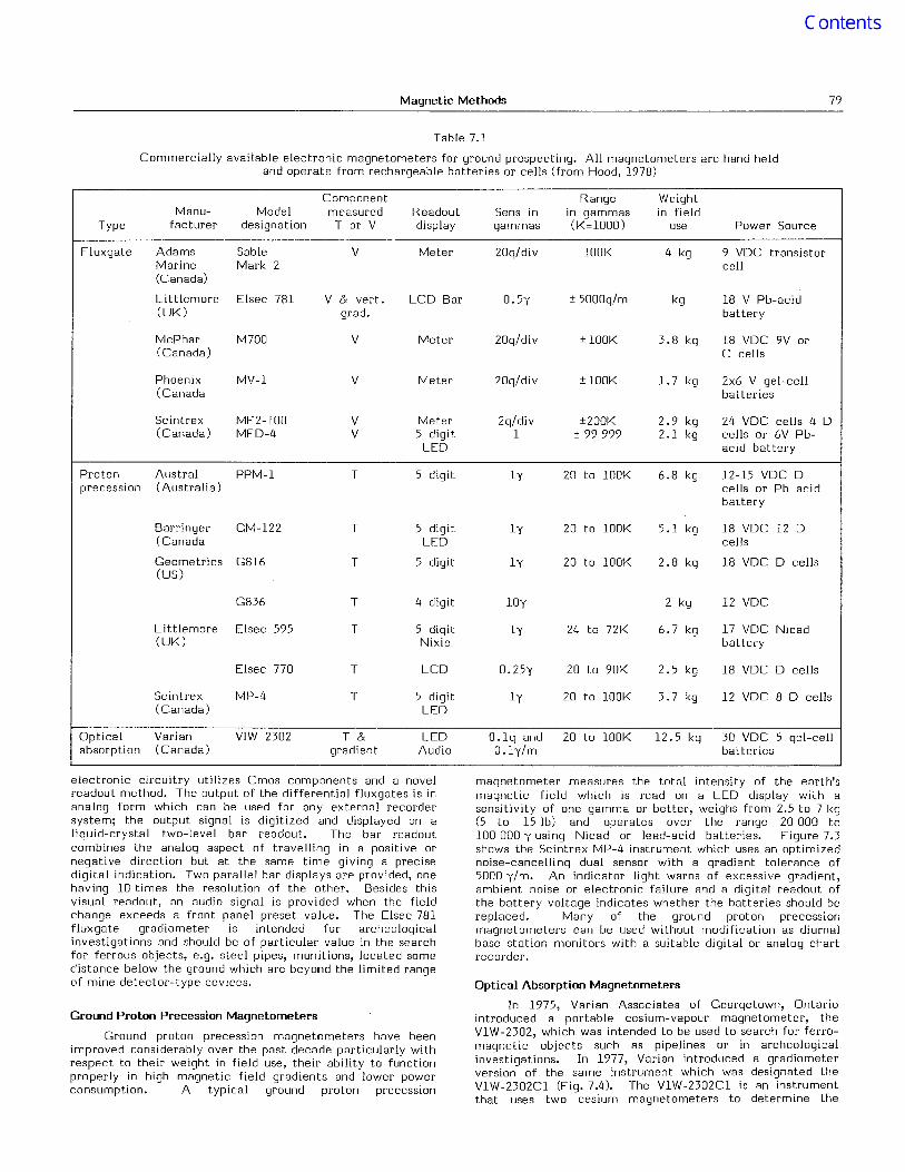
Table 7.1

Commercially available electronic magnetometers for ground prospecting. All magnetometers are hand heldand operate from rechargeable batteries or cells (from Hood, 1978)

79

Component Range WeightManu- Model measured Readout Sens in in gammas in field

Type facturer designation T or V display gammas (K=1000) use Power Source

Fluxgate Adams Sable V Meter 20q/div lOOK 4 kg 9 VDC transistorMarine Mark 2 cell(Canada)

Littlemore Elsec 781 V & vert. LCD Bar 0.5y ± 5000q/m kg 18 V Pb-acid(UK) grad. battery

McPhar M700 V Meter 20q/div ± lOOK 3.8 kg 18 VDC 9V or(Canada) C cells

Phoenix MV-l V Meter 20q/div ±100K 1.7 kg 2x6 V gel-cell(Canada batteries

Scintrex MF2-100 V Meter 2q/div ±200K 2.9 kg 24 VDC cells 4 D(Canada) MFD-4 V 5 digit 1 ± 99 999 2.1 kg cells or 6V Pb-

LED acid battery

Proton Austral PPM-l T 5 digit ly 20 to lOOK 6.8 kg 12-15 VDC Dprecession (Australia) cells or Pb acid

battery

Barringer GM-122 T 5 digit ly 20 to lOOK 5.1 kg 18 VDC 12 D(Canada LED cells

Geometries G816 T 5 digit ly 20 to lOOK 2.8 kg 18 VDC D cells(US)

G836 T 4 digit lOy 2 kg 12 VDC

Littlemore Elsec 595 T 5 digit ly 24 to 72K 6.7 kg 17 VDC Nicad(UK) Nixie battery

Elsec 770 T LCD 0.25y 20 to 90K 2.5 kg 18 VDC D cells

Scintrex MP-4 T 5 digit ly 20 to lOOK 3.7 kg 12 VDC 8 D cells(Canada) LED

Optical Varian VIW 2302 T & LED O.lq and 20 to lOOK 12.5 kg 30 VDC 5 gel-cellabsorption (Canada) gradient Audio O.ly/m batteries

electronic circuitry utilizes Cmos components and a novelreadout method. The output of the differential flux gates is inanalog form which can be used for any external recordersystem; the output signal is digitized and displayed on aliquid-crystal two-level bar readout. The bar readoutcombines the analog aspect of travelling in a positive ornegative direction but at the same time giving a precisedigital indication. Two parallel bar displays are provided, onehaving 10 times the resolution of the other. Besides thisvisual readout, an audio signal is provided when the fieldchange exceeds a front panel preset value. The Elsec 781flux gate gradiometer is intended for archeologicalinvestigations and should be of particular value in the searchfor ferrous objects, e.g. steel pipes, munitions, located somedistance below the ground which are beyond the limited rangeof mine detector-type devices.

Ground Proton Precession Magnetometers

Ground proton precession magnetometers have beenimproved considerably over the past decade particularly withrespect to their weight in field use, their ability to functionproperly in high magnetic field gradients and lower powerconsumption. A typical ground proton precession

magnetometer measures the total intensi ty of the earth'smagnetic field which is read on a LED display with asensitivity of one gamma or better, weighs from 2.5 to 7 kg(5 to 15 Ib) and operates over the range 20 000 to100 000 Y using Nicad or lead-acid batteries. Figure 7.3shows the Scintrex MP-4 instrument which uses an optimizednoise-cancelling dual sensor with a gradient tolerance of5000 y/m. An indicator light warns of excessive gradient,ambient noise or electronic failure and a digital readout ofthe battery voltage indicates whether the batteries should bereplaced. Many of the ground proton precessionmagnetometers can be used without modification as diurnalbase station monitors with a suitable digital or analog chartrecorder.

Optical Absorption Magnetometers

In 1975, Varian Associates of Georgetown, Ontariointroduced a portable cesium-vapour magnetometer, theVI W-2302, which was intended to be used to search for ferro­magnetic objects such as pipelines or in archeologicalinvestigations. In 1977, Varian introduced a gradiometerversion of the same instrument which was designated theVI W-2302Cl (Fig. 7.4). The VI W-2302Cl is an instrumentthat uses two cesium magnetometers to determine the

80 Peter J. Hood et at.

Figure 7.1. McPhar M700 fluxgate magnetometer withstrap around operator's neck, being operated on the Cavendishgeophysical test range, southwestern Ontario; McPharInstrument Corp., WiZZowdale, Ontario. (GSC 202228-G)

magnitude of the magnetic field intensity at two pointsspaced 2 m apart. By subtracting the two measured values, agradient of the total field intensity can be determined. Thesensitivity of the gradient measurement is ± 0.1 y/2 m andthe range is ± 9000 y/2 m. The instrument is also designed towork in the so-called variometric mode whereby one Cssensor is stationary while the other, connected via a singlecoaxial cable, is used as a mobile sensor. In this mode a verydetailed survey of an area may be conducted with the resultsbeing independent of time-varying components of the earth'smagnetic field, i.e. diurnal changes and micropulsations.Each of the two Varian cesium sensors can also be used forthe total field measurements. In this mode of operation, themagnitude of the magnetic field intensity can be measuredover the range of 20 000 to 100 000 y, which permits theinstrument to be used for magnetic surveys in any part of theworld. The sensitivity of the measurements is ±0.1 yand theabsolute accuracy is ± 0.5 y. In all three modes of operation(gradiometer/variometer/total field magnetometer) theresults are displayed in the form of a 6-digit number by a7 segment incandescent display on the 2.1 kg console. Thedisplay is updated 2 times per second. In addition to thevisual display, an audio output is available whose frequency is7 Hz/y in the total field mode and 7 Hz per 1 y/2 m in thegradiometric mode. The audio display permits a rapid surveyfor localized magnetic anomalies due to buried artifacts. The

Figure 7.2. Elsec 781 digital fZuxgate gradiometer;Littlemore Scientific Engineering Co., Oxford, U.K.(GSC 203492-0)

visual display update time is limited by the human response.The instrument takes measurements at the rate of 11 timesper second and each of the measurements takes0.045 seconds. This information is available in the digital(BCD) form or analog form (potentiometric or galvanometric)for the recording version of the instrument. The VarianVIW-2302Cl portable gradiometer is powered by 5 gelrechargeable batteries connected in series (providing 30 V)for periods of up to 6 hours before the batteries have to berecharged; the temperature operating range is 0° to 50°C.

Instrumentation for Magnetic Property Measurements

It is often useful to investigate the magnetic propertiesof a rock formation to ascertain whether it has sufficientmagnetization to produce a given anomaly or whether thedirection of the magnetization vector differs markedly fromthat of the present earth's field e.g. is reversed. Themagnetization (J) of a given rock formation is due to twocomponents, namely the' induced and the remanentmagnetization (R). These are vectors and the inducedmagnetization is accurately aligned in the direction of theearth's magnetic field (T).

Magnetic Methods 81

Figure 7.3. Scintrex MP-4 direct-reading proton precessionmagnetometer; Scintrex Ltd., Toronto, Ontario.(GSC 202228-E)

Thus "3 = kT + Rwhere k is the susceptibility of the rock formation. Thus inorder to ascertain the total magnetization of a rockformation it is necessary to measure both the susceptibilityand the remanent magnetization vector.

Susceptibility Meters

The preferred technique in measuring the susceptibilityof a given rock formntion is to carry out in situmeasurements because this physical parameter is somewhatvariable and a representative determination cannot normallybe made from a few hand specimens.

Table 7.2 lists the susceptibility meters which arepresently available. Several portable susceptibility metershave appeared in the last decade. One example is the ElliotPP-ZA instrument (Fig. 7.5) which weighs 0.5 kg and may beused to measure the susceptibility of hand and drill coresamples or for in situ measurements on outcropping rockformations. The direct digital readout of susceptibility totwo significant figures over the range 100 x 10- 6 to 99000x 10- 6 cgsu (1244 X 10- 3 SIu) maybe obtained with aresolution of 100 x 10- 6 cgsu (0.13 x 10- 3 SIu) by pushing abutton. The instrument may also be calibrated in percentagemagnetite equivalents for the direct logging of drill core formagnetite content.

Figure 7.4. V1W-2302Cl cesium gradiometer; VarianAssociates, Georgetown, Ontario. (GSC 203492-T)

Figure 7.5. Elliot PP-2A susceptibility meter; ElliotGeophysical Co., Tucson, Arizona. (GSC 203492-5)

Magnetic Methods 83

timess took only 10 minutes. The JR-2 had a sensitivity of 4x 10- Am-I. It did not require any special laboratoryconditions. The LAM-l astatic magnetometer was capable ofmeasuring the remanence, susceptibility, and susceptibilityanisotropy using irregular and large sized rock samples. Thesensitivity of the LAM-l was about 1.6 x 10-5 Am-I, i.e.2 x 10- 7 De. In 1973, the range of LAM astaticmagnetometers was increased by the introduction of threenew models. The basic, simplest version LAM-2 measures theastatic system deflection by a light beam spot on a graduatedscale with sensiti vity 4 x 10- 15 to 6 X 10- 6 Am-I scale division(5 x 10- 7 to 5 X 10- 8 De/scale division). The LAM-3incorporates an electronic negative feedback loop and systemdeflection is displayed on an analog indicator. This gives ashorter setting time, stabilizes the sensiti vit y and allowssimple range selection. A digital output device converts theLAM-3 to a LAM-3D which permits automatic data recordingfor computer handling. The LAM-4 has automatic rangingwhich further shortens the measuring time. The LAM-3 andLAM-4 have 7 sensitivity ranges from 8 x 10- 4 to 8 X 10- 1

Am-I (1 x 10- 5 to 1 X 10- 2 De/fsd). Each LAM is providedwith an orthogonal manipulator that will take irregularsamples of up to 10 cm diameter; a micro lamp for smallsamples is also provided so that measurements are quicklycarried out.

In 1974, the Institute of Applied Geophysics in Brno,Czechoslovakia commenced delivery of a digital version oftheir JR series (JR-2 and the subsequent JR-3) of spinnermagnetometers. The new instrument, designated UGF-JR4has digital indication of two simultaneous components ofremanent magnetic polarization and parallel BCD output fordirect computer processing of measured data. Samples maybe cubes 20 x 20 x 20 mm or cylinders 25.4 mm diameter by22 mm length. Cylinders are measurable with axis vertical orhorizontal. The major improvements incorporated in the JR- 4rock magnetometer include increased sensitivity, a widermeasuring range, simpler measuring procedure, automaticcompensation for magnetic moment of sample holder, higheraccuracy, and shorter measuring time. Some of the featuresof the new instrument are automatic compensation for themagnetic moment of the sample holder, use of phototransistors instead of permanent magnets to obtain thereference signal, and an automatic stopping of the samplerotation at the end of integration time. The most sensitivemeasuring range covers 0-9.99 picoteslas with a sensiti vity of1 pT for an inteqration time of 100 seconds.

Figure 7.7. Schonstedt PSM-l remanent magnetometer forfield measurements; Schonstedt Instrument Co., Reston,Virginia. (eSC 202228-F)

A portable instrument designated the PSM-l (Fig. 7.7)has been developed by Schonstedt Instrument Company ofReston, Virginia, in which the remanent magnetization ofirregularly-shaped rock specimens may be measured. Full­scale ranges of 10- 4 to 1 emu (10- 1 to 10 3 Am-I) permit themeasurement of virtually all igneous rocks and many types ofsediments with an accuracy of ± 10% of moment and ± 5%direction angle. Schonstedt also manufactures a range oflaboratory spinner magnetometers for more accurateremanent magnetism measurements.

Superconducting quantum interference device (Squid)sensors have also been developed for use in rock magnetismmeasurements. The interested reader is referred to anexcellent review of the topic by Goree and Fuller (1976) fordescriptions of the theory and design of the Squidinstrumentation.

Drillhole Logging Instrumentation

F or iron-ore prospecting, the measurement of themagnetic parameters of rock formations through whichdrillholes pass are carried out using susceptibility loggingequipment or by the use of three-component fiuxgatemagnetometers. In 1974, Zablocki described the magneticsusceptibility system being used by the U.S. Steel Corporationat the Minntac open-pit taconite mine in northern Minnesotafor short blast holes 40-60 feet (12-18 m) in depth with adiameter of 12.25 in. (31 cm). Figure 7.8 shows a schematicdiagram of the system which uses an air-cored multi-turninduction coil connected to one arm of an inductance bridgeand designed using an operational amplifier so that there wasconstant current through the induction coil. The system hada capability of measuring the Fe content in the drillholes witha standard error of ± 1.2 weight per cent Fe, and wasconsidered to be especially useful in establishing cut-offboundaries between ore and waste. In situ bulk measurementsare much preferable to laboratory measurements of muchsmaller volumes using drill core.

In recent years much effort has been devoted in Swedento the development of a reliable drillhole fiuxgatemagnetometer which would be useful for the detection ofiron-ore deposits. In 1969, ABEM introduced a new version ofthe Swedish three-component drillhole magnetometer for EX(36 mm) holes designated the HBM 4 (Fig. 7.9). Thistransistorized instrument measures three orthogonalmagnetic components as well as dip angle down to 1200 m(3600 ft.). The measurements have an accuracy of 50 y withinthe range ± 100 000 Y and 150 y in the range ± 300 000 y. Thedip of the hole is measurable from +90 0 (horizontal) to -40 0

with an accuracy of 0.5 0• The major difference from the

previous model is the electronic switching of fiuxgate probesinstead of servomotor changeover.

Lantto (1973) has presented a general interpretationprocedure for magnetic logging data called the characteristiccurve method. This method is based on the characteristicpoints of a profile where either the horizontal or verticalfield components are zero. Standard curves are given in thepaper for models which can be represented by two parallelinfinite line poles (long tubular bodies) or dipoles (rod-shapedbodies). The standard curves were applied to determining thedepth of the bottom of an iron ore deposit at the Dtanmakimine in Finland using characteristic points located on thesurface and in two boreholes.

Airborne Magnetometers

Table 7.3 shows the airborne magnetometers which arecommercially available at the time of writing. Direct­reading proton precession magnetometers are now in commonuse for standard sensitivity aeromagnetic surveys in inboard

Magnetic Methods 83

timess took only 10 minutes. The JR-2 had a sensitivity of 4x 10- Am-I. It did not require any special laboratoryconditions. The LAM-l astatic magnetometer was capable ofmeasuring the remanence, susceptibility, and susceptibilityanisotropy using irregular and large sized rock samples. Thesensitivity of the LAM-l was about 1.6 x 10-5 Am-I, i.e.2 x 10- 7 De. In 1973, the range of LAM astaticmagnetometers was increased by the introduction of threenew models. The basic, simplest version LAM-2 measures theastatic system deflection by a light beam spot on a graduatedscale with sensiti vity 4 x 10- 15 to 6 X 10- 6 Am-I scale division(5 x 10- 7 to 5 X 10- 8 De/scale division). The LAM-3incorporates an electronic negative feedback loop and systemdeflection is displayed on an analog indicator. This gives ashorter setting time, stabilizes the sensiti vit y and allowssimple range selection. A digital output device converts theLAM-3 to a LAM-3D which permits automatic data recordingfor computer handling. The LAM-4 has automatic rangingwhich further shortens the measuring time. The LAM-3 andLAM-4 have 7 sensitivity ranges from 8 x 10-" to 8 X 10- 1

Am-I (1 x 10- 5 to 1 X 10- 2 Oe/fsd). Each LAM is providedwith an orthogonal manipulator that will take irregularsamples of up to 10 cm diameter; a microlamp for smallsamples is also provided so that measurements are quicklycarried out.

In 1974, the Institute of Applied Geophysics in Brno,Czechoslovakia commenced delivery of a digital version oftheir JR series (JR-2 and the subsequent JR-3) of spinnermagnetometers. The new instrument, designated UGF-JR4has digital indication of two simultaneous components ofremanent magnetic polarization and parallel BCD output fordirect computer processing of measured data. Samples maybe cubes 20 x 20 x 20 mm or cylinders 25.4 mm diameter by22 mm length. Cylinders are measurable with axis vertical orhorizontal. The major improvements incorporated in the JR- 4rock magnetometer include increased sensitivity, a widermeasuring range, simpler measuring procedure, automaticcompensation for magnetic moment of sample holder, higheraccuracy, and shorter measuring time. Some of the featuresof the new instrument are automatic compensation for themagnetic moment of the sample holder, use of phototransistors instead of permanent magnets to obtain thereference signal, and an automatic stopping of the samplerotation at the end of integration time. The most sensitivemeasuring range covers 0-9.99 picoteslas with a sensiti vity of1 pT for an inteqration time of 100 seconds.

Figure 7.7. Schonstedt PSM-l remanent magnetometer forfield measurements; Schonstedt Instrument Co., Reston,Virginia. (eSC 202228-F)

A portable instrument designated the PSM-l (Fig. 7.7)has been developed by Schonstedt Instrument Company ofReston, Virginia, in which the remanent magnetization ofirregularly-shaped rock specimens may be measured. Full­scale ranges of 10-" to 1 emu (10- 1 to 10 3 Am-I) permit themeasurement of virtually all igneous rocks and many types ofsediments with an accuracy of ± 10% of moment and ± 5%direction angle. Schonstedt also manufactures a range oflaboratory spinner magnetometers for more accurateremanent magnetism measurements.

Superconducting quantum interference device (Squid)sensors have also been developed for use in rock magnetismmeasurements. The interested reader is referred to anexcellent review of the topic by Goree and Fuller (1976) fordescriptions of the theory and design of the Squidinstrumentation.

Drillhole Logging Instrumentation

For iron-ore prospecting, the measurement of themagnetic parameters of rock formations through whichdrillholes pass are carried out using susceptibility loggingequipment or by the use of three-component fiuxgatemagnetometers. In 1974, Zablocki described the magneticsusceptibility system being used by the U.S. Steel Corporationat the Minntac open-pit taconite mine in northern Minnesotafor short blast holes 40-60 feet (12-18 m) in depth with adiameter of 12.25 in. (31 cm). Figure 7.8 shows a schematicdiagram of the system which uses an air-cored multi-turninduction coil connected to one arm of an inductance bridgeand designed using an operational amplifier so that there wasconstant current through the induction coil. The system hada capability of measuring the Fe content in the drillholes witha standard error of ± 1.2 weight per cent Fe, and wasconsidered to be especially useful in establishing cut-offboundaries between ore and waste. In situ bulk measurementsare much preferable to laboratory measurements of muchsmaller volumes using drill core.

In recent years much effort has been devoted in Swedento the development of a reliable drillhole fiuxgatemagnetometer which would be useful for the detection ofiron-ore deposits. In 1969, ABEM introduced a new version ofthe Swedish three-component drillhole magnetometer for EX(36 mm) holes designated the HBM 4 (Fig. 7.9). Thistransistorized instrument measures three orthogonalmagnetic components as well as dip angle down to 1200 m(3600 ft.). The measurements have an accuracy of 50 y withinthe range ± 100 000 Y and 150 y in the range ± 300 000 y. Thedip of the hole is measurable from +90 0 (horizontal) to -40 0

with an accuracy of 0.5 0• The major difference from the

previous model is the electronic switching of fiuxgate probesinstead of servomotor changeover.

Lantto (1973) has presented a general interpretationprocedure for magnetic logging data called the characteristiccurve method. This method is based on the characteristicpoints of a profile where either the horizontal or verticalfield components are zero. Standard curves are given in thepaper for models which can be represented by two parallelinfinite line poles (long tubular bodies) or dipoles (rod-shapedbodies). The standard curves were applied to determining thedepth of the bottom of an iron ore deposit at the Otanmakimine in Finland using characteristic points located on thesurface and in two boreholes.

Airborne Magnetometers

Table 7.3 shows the airborne magnetometers which arecommercially available at the time of writing. Direct­reading proton precession magnetometers are now in commonuse for standard sensitivity aeromagnetic surveys in inboard

84 Peter J. Hood et al.

RECORDER

PHASEDETECTORSYSTEM

NULLCONDITIONS

Lx = R1R3C

Rx = R1R3R2

Figure 7.9. ABEM three-component {luxgatemagnetometer for drillhole logging; Atlas Copco ABEM AB,Stockholm, Sweden. (eSC 203492-U)

TOP VIEW

SIDE VIEW

TYPE I INDUCTION COIL

Figure 7.8. Magnetic susceptibility drillhole logging system(Zablocki, 1974).

installations and their sensitivity is mostly 1.0 gamma orbetter. However, the use of fluxgate magnetometers persistsperhaps because they produce a continuous analog outputinstead of a stepped one and this is preferred by manymagnetic interpreters who use graphical interpretation

techniques. The range of airborne proton precesslOn magnet­ometers is typically 20 000 to 100 000 Y and this permits theiruse worldwide except over the most strongly magnetized ironformations.

During 1969, Geometries introduced their Model G-803direct-reading airborne proton precession magnetometer(Fig. 7.10). The complete 22.3 kg aeromagnetic surveysystem consists of a 6.4 kg magnetometer console in astandard 19 inch rack, a 5.5 kg 13 em chart recorder, and abird and towing-system weighing 10.5 kg. The range of theinstrument is 20 000 to 100 000 Y in 10 manually-selectedoverlapping ranges. The sensitivity of the standardinstrument is 1 y at a sampling rate of 1 second controlledeither by external or internal automatic triggers or manually.Other options are available such as a 0.5 y magnetometer withan 0.8 second sampling rate. The total field output of theinstrument may be recorded digitally and/orpotentiometrically or galvanometric analog recordingemployed.

Gam Service Ltd. of Grenoble, France, which is part ofthe French Atomic Energy Commission, is manufacturing anOverhauser proton precession magnetometer, the MPPEIol,which has a 0.01 y sensitivity at a 1 second sampling interval.The range of the 27 kg magnetometer is 20 000 to80 000 y. Both analog and BCD digital outputs are provided.The instrument has been used for aeromagnetic surveys andas a differential magnetometer for archeologicalinvestigations (Collin et aI., 1973); it is readily apparent thatit would be well suited for use in a vertical gradiometeraeromagnetic survey system.

Magnetic Methods

Table 7.3

Airborne magnetometers available for purchase. All magnetometers measure the total intensity ofthe earth's magnetic field, have visual displays, and are direct reading

Magnet- Range in Sampling rate Readout Powerometer Manu- Max sens gammas for maximum A=Analog Require-

and type facturer Model No. in gammas (K=1000) sensitivity D=Digital ments Weight (kg)

Proton Barringer AM 123 ly 20-100K 1 sec A & D 12-30VDC 9.1 (incl. chartprecession- (Canada) 5A polarize recorder)directreading Geometrics G 803 ly 20-100K 1 sec A & D 22-32VDC 6.4

(US) 150Waverage

Littlemore Elsec 5951 ly 24-72K 1. 2 sec A & D 20-2BVDC 25(UK)

Elsec 7702 ly 20-90K 2 sec A 20-2BVDC 7

Sander NPM-5 o.1y 20-100K 1 sec A & D 2BVDC lA 5 (console)(Canada) + 7A

polarize

Scintrex MAP-4 ly 20-100K 0.5 sec A & D 24-30VDC 6 (console)(Canada) 3.5A max. 3 (sensor )

Sonotek IGSS/SDS 0.1Y 15-100K 1 sec A & D 2BVDC(Canada) systems

Varian V-85 0.1Y 20-100K 1 sec A & D 28VDC 4A 7.7(Canada polarize

Overhauser Gam Service MPPEI0l O.Dly 20-BOK A & D 12&2BVDC 27(France) 2.5A

85

Figure 7.10. Geometries G803 proton precession airbornemagnetometer; Geometries Inc., Sunnydale, California(GSC 203492-R)

Aeromagnetic Gradiometers

The use of optical absorption magnetometers foraeromagnetic surveying appears to have been mostly confinedto petroleum exploration with the exception of theexperimental airborne system installed inboard on aBeechcraft BBO aircraft of the Geological Survey of Canada.During the middle 70's the system was modified by theaddition of a second boom (Fig. 7.11) so that the verticalgradient of the earth's total field could be measured directly(Sawatzky and Hood, 1975). The successful development ofthis system was only made possible by the use of two acti vemagnetic compensation systems which are manufactured byCanadian Aviation Electronics of Montreal. The verticalseparation of the single-cell self-orienting optical absorptionmagnetometers in the two booms is approximately 2 metresand the system is designed for gradiometer surveys ofPrecambrian Shield areas rather than for petroleumexploration.

With regard to the desirable sensitivity formagnetometers to be used in an inboard vertical gradiometersystem, two main factors enter into the consideration: 1) thebasic sensitivity of the magnetometers themselves, and2) their vertical separation. It is clear from the results of thesurveys flown at 500 feet (152 m) over the CanadianPrecambrian Shield by the Geological Survey of Canada thata contour interval of at least 0.025 y/m should be utilized indelineating magnetic gradient anomalies. Anomalies of thisamplitude commonly extend across several flight lines (seeFig. 2 in Coope, 1979, where the spacing of the N-S flightlines is 1000 ft. (305 m)) and therefore reflect the presence ofunderlying geological features having a low magnetizationcontrast with respect to the surrounding rocks. The ratiobetween the basic sensitivity of the survey magnetometer and

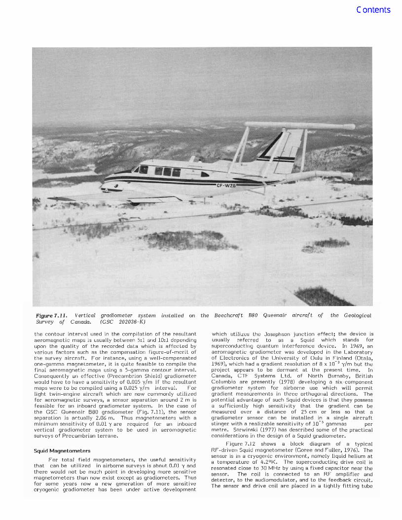
Figure 7.11.Survey of

Vertical gradiometer systemCanada. (GSC 202036-K)

install ed on the Beechcraj't BBO Queenair aircraft of the Geological

the contour interval used in the compilation of the resultantaeromagnetic maps is usually between 5:1 and 10:1 dependingupon the quality of the recorded data which is affected byvarious factors such as the compensation figure-of-merit ofthe survey aircraft. For instance, using a well-compensatedone-gamma magnetometer, it is quite feasible to compile thefinal aeromagnetic maps using a 5-gamma contour interval.Consequently an effective (Precambrian Shield) gradiometerwould have to have a sensitivity of 0.005 y/m if the resultantmaps were to be compiled using a 0.025 y/m interval. Forlight twin-engine aircraft which are now commonly utilizedfor aeromagnetic surveys, a sensor separation around 2 m isfeasible for an inboard gradiometer system. In the case ofthe GSC Queenair BBo gradiometer (Fig. 7.11), the sensorseparation is actually 2.06 m. Thus magnetometers with aminimum sensitivity of 0.01 yare required for an inboardvertical gradiometer system to be used in aeromagneticsurveys of Precambrian terrane.

Squid Magnetometers

For total field magnetometers, the useful sensitivitythat can be utilized in airborne surveys is about 0.01 y andthere would not be much point in developing more sensitivemagnetometers than now exist except as gradiometers. Thusfor some years now a new generation of more sensitivecryogenic gradiometer has been under active development

which utilizes the Josephson junction effect; the device isusually referred to as a Squid which stands forsuperconducting quantum interference device. In 1969, anaeromagnetic gradiometer was developed in the Laboratoryof Electronics of the University of Oulu in Finland (Otala,1969), which had a gradient resolution of B x 10- 3 y/m but theproject appears to be dormant at the present time. InCanada, CTF Systems Ltd. of North Burnaby, BritishColumbia are presently (197B) developing a six-componentgradiometer system for airborne use which will permitgradient measurements in three orthogonal directions. Thepotential advantage of such Squid devices is that they possessa sufficiently high sensitivity that the gradient can bemeasured over a distance of 25 cm or less so that agradiometer sensor can be installed in a single aircraftstinger with a realizable sensiti vity of 10- 5 gammas permetre. Sarwinski (1977) has described some of the practicalconsiderations in the design of a Squid gradiometer.

Figure 7.12 shows a block diagram of a typicalRF-driven Squid magnetometer (Goree and Fuller, 1976). Thesensor is in a cryogenic environment, namely liquid helium ata temperature of 4.2°K. The superconducting drive coil isresonated close to 30 MHz by using a fixed capacitor near thesensor. The coil is connected to an RF amplifier anddetector, to the audiomodulator, and to the feedback circuit.The sensor and drive coil are placed in a tightly fitting tube

Magnetic Methods 87

ERROR DETECTION AND CORRECTION ERROR DETECTION AND CORRECTION

l.m~,", "mu", ,"mm~M' me<J1

POST-FLIGHT RECOVERED TRACK DATA(line number. co-ordinates of pointson track and fiducial,)

1

DATA RECORDED IN-FLIGHT(line number,magnetic measurementand fi duci a1 numbers)

LOW- FREQUENCYAMPLIFIER ANDFIL TER

FEEDBACK CIRCUIToDRIVE ANDSENSE COIL

MAGNETOMETERSENSOR

- .CRYOGENIC ENVIRONMENT

OUTPUTSIGNAL

1

With the advent of the high sensitivity opticalabsorption magnetometer, the use of paper recording chartsbecame altogether impractical. Were a strip chart recorderto be calibrated so as to be readable at the full sensitivity ofan optical absorption magnetometer, then over a largeanomaly the datum on the chart would be reset as much as1000 times, producing an unusable record.

It therefore became necessary to employ a recordingmedium whose sensitivity matched that of the newmagnetometer, and one advantageous for the less sensitiveinstruments. A digital recording system has, for all practicalpurposes, an unlimited sensitivity. This phenomenon of aneed to change from analog to digital methods was not, ofcourse, restricted to aeromagnetic work. It was widespreadthroughout the whole of the science and technology sector.The reason was that, although the early digital systems weremore expensive than analog ones, each increase in sensitivityby an order of magnitude required a small fixed cost for adigital system ("add one more digit") whereas the increase foran analog system may require a corresponding order ofmagnitude increase in cost ("make the chart paper andrecorder ten times wider"). A further potential advantagewas offered by the lower weight, and fewer moving parts ofprincipally electronic devices. Thus direct inflight digitalrecording began to be adopted by the aerogeophysical surveyindustry and the need for digital compilation systems arose.

Figure 7.13 summarizes the main processes ofaeromagnetic compilation whether manual or digital. Thelevelling process removes the nongeological datum variationsfrom line to line caused by inexact flight altitude, diurnalvariation of the earth's magnetic field and other causes.

In the manual compilation process, magnetic values atthe intersection points of a "levelling network" formed by thecontrol and the main traverse lines were picked off theanalog chart. Levelling adjustments were determinedmanually and the adjustment values marked on the analogchart at the intersections of the control and traverse lines.These points were then joined by straight lines drawn on thechart to establish a corrected datum. The magnetic profileswere then intercepted at the map contour interval required,

Figure 7.12. Block diagram of the circuitry for a RF-driven Squid magnetometer (from Goree and Fuller, 1976).

on which the superconducting field coil is wound. Thisassembly is then placed in a superconducting shield to isolatethe sensor from all magnetic field changes except that fromthe field coil. The field coil of the standard sensor requires acurrent of about 0.3 jl A to change the flux linking theSquid by one flux quantum, which is a field change of1 y for a 1.6-mm diameter sensor. Typical sensors arecapable of a resolution of one part in 1500 of a flux quantum.Thus the peak-to-peak current resolution. is 0.2 nA, whichgives a field sensitivity at the sensor of 7 x 10- 4 y.

Digital Data Acquisition Systems

Digital recording on magnetic tape of the total fieldand doppler and altitude information is now the standard dataacquisition technique for aeromagnetic survey data, and thispermits the subsequent compilation of the digital data to becarried out using the computer.

For a description of the various digital data acquisitionsystems in current use in the industry, the reader is referredto the annual reviews published by Hood during the reviewperiod (see for instance Hood, 1972, 1973, 1976, 1977).

DIGITAL COMPILATION OF AEROMAGNETICSURVEY DATA

Great progress has been made in the last decade indigital compilation techniques and all the major airbornegeophysical survey companies now possess their own in-housecomputer hardware and software capability. This has comeabout partly as a result of the introduction of opticalabsorption magnetometers which required digital-recordingsystems to avoid the dynamic range recording problem withhigh resolution data, and of a general realization of the factthat digital compilation techniques would produce moreobjecti ve results and would permit much greater versatility indata processing operations.

Fifteen years ago with the fluxgate and protonprecession magnetometers then in use, a paper strip chartabout 25 cm in width provided adequate resolution forrecording the aeromagnetic field variations. However, withsuch a chart calibrated to allow the trace to be read to theprecision of the instrument, the chart datum would beautomatically reset perhaps 20 times in covering a very largeanomaly, making the chart difficult to read in high gradientareas.

Figure 7.13.

INTERPOLATE CONTOURS BETWEEN MAGNETICVALUES ALONG THE FLIGHT LINES

1MAP OF AEROMAGNETIC TOTAL FIELD

Basic processes of aeromagnetic compilation.

88 Peter J. Hood et al.

usually 10 y, using the datum. These intercepted values werethen transcribed onto a flight path manuscript and handdrawn contours visually interpolated between the flight lines.With the advent of digital recording, computer programs weredeveloped to carry out those manual operations previouslyperformed on the chart. A minimal software system wouldrequire a routine to retrieve the value of the magnetic fieldat the manually determined levelling network points, aroutine to make a linear interpolation between these points toproduce the computer equivalent of the chart datum, and aroutine to output corrected values as the difference betweenthe originally measured value and the datum at the requiredcontour interval. These values could then be transcribed ontothe flightpaUi manuscript and contoured manually as before.

Once having been required to employ the computer, theadvantages and indeed necessities of developing beyond thisminimal software system became obvious. An earlyrequirement was the need to be able to determine errors andaberrations in the digitally recorded data. Compared withthe highly visible trace on the strip chart, errors in thedigitally recorded data were less easy to detect.

The most direct and familiar way to present the datafor inspection being the form in which it had previously beenrecorded, namely, as an analog profile, development movedinto the field of computer graphics. This allowed the digitaldata to be output in analog form and inspected for obviouserrors in exactly the same manner that the strip chart hadbeen treated previously.

Access to computer graphics having been gained, theobvious next step was automation of the laborioustranscription process. This, however, would have resulted inan awkward hybrid process unless the base map of the flightpath could also be produced by computer.

Another necessity then presented itself, namely theneed to employ digitizing facilities. Although recovered bymanual methods, flight path data once digitized, can besubmitted to computer automated processes and thetranscription of the data to the flight path base map madecompletely automatic.

Up to this point the production of computer automatedcompilation software had been a relatively straightforwardprocess, the level of software sophistication required beingrelatively low. At this point however the required complexityof the software increased significantly.

The acquisition sequence of the in-flight data, andtherefore the order of the data on the magnetic tape, isdetermined by logistical and economic considerations. Linesare not flown all in the same direction and in strictgeographical order across the survey area as this wouldrequire a prohibitively high proportion of nonproductive flyingmerely to position the aircraft for each survey line. Thesequence of digitization of recovered flight path data islikewise governed by practical considerations. Unless themap area of the survey at the recovery scale is small enoughto fit onto the digitizing table, then flight lines must bedigitized map sheet by map sheet. Hence a line which existson the in-flight data tape as a continuous unbroken sequenceof records, will exist on the digitized flight path data tape asa series of map sheet-sized segments separated by segmentsof other lines. In order to bring the two data sets together, itis necessary to submit them, either or both, to a complex"sort-merge" process. Once software for this purpose hasbeen implemented, then automatic transcription of in-flightdata onto flight path base maps can be carried out.

All the previously mentioned processes, though complexin some cases, are eminently suited for computer automation,consisting as they do of a sequence of well defined andrepetitive processes. Such is not the case with the levellingand contouring stages.

Although the basics of the levelling process can be welldefined many further factors dependent upon the skill andexperience of the map compiler enter into the process as it isexecuted. The compiler will seek sources other than the dataimmediately at hand to explain and resolve dubious levellingcorrections. Certain results will not "feel right" to theexperienced compiler and special attention would be paid tothese cases. The computer is not, of course, capable of suchbeneficial digressions from the specified task.

Gridding and Contouring

Similarly in the case of contouring, although thecomputer is capable of doing an excellent job with properlysampled data, if the data are undersampled (e.g. if the flightline spacing is too wide for the chosen flight altitude) thenthe computer does its best to produce a map which bestrepresents the data as sampled - namely a poor map. Withhand contouring the draughtsman would decide upon anappropriate trend and string the contours along this trend asthough they were smoothly and well defined along theirlength. The resulting product has a pleasing, albeitpotentially deceiving, appearance.

Figures 7.14a, b, c demonstrate just how appearancescan be deceiving. All three maps are computer-contouredsegments of an aeromagnetic gradiometer survey flown at500 ft. (150 m) altitude with 500 ft. (150 m) line spacing.They all cover the same area of the survey but Figure 7.14awas contoured from all the original data. Figure 7.14b wascontoured from every second flight line only and Figure 7.14cwas contoured from every fourth flight line only. HenceFigures 7.14b and 7.14c represent the end product as it wouldappear had the survey been flown at 1000 (305 m) and 2000 ft.(610 m) line spacings respectively.

It must be noted that the gridding and contouringprograms employed ensure that the contour positions areexact to within 0.01 cm where the contours pass over theflight lines. The contour positions between flight lines aresomewhat conjectural whether contoured by man or machine,but with undersampled data, manual contours appear morereasonable. Figure 7.14c clearly exhibits the typical,undesirable features of m'achine-contoured, undersampleddata. Namely isolated "potato" anomalies (or magneticboudinage) elongated at right angles to the flight lines andthe tendency for contours which cross several flight lines toundulate between the flight lines rather than link up theflight line contour intersection points with a smoothcontinuous curve, as is the case with manual contours.

Figures 7.14a and 7.14b, however, do not clearly exhibitthe symptoms of undersampling. In both cases, contours crossthe flight lines as smooth continuous curves and elongatedtrends are shown at sharp angles to the flight line direction ­symptomatic of good sampling.

The interesting consequence is, however, that the500 ft. (150 m) line spacing, which we will regard as theaccurate depiction of the magnetic field variations, shows aseries of four-parallel "ridges" separated by "troughs" runningapproximately 15 0 east of north, whereas the less wellsampled data in Figure 7.14b exhibits only one such, butstronger, feature with a very emphatic cross-cutting troughoriented about 20 0 west of north. This feature is clearlyspurious, but so well defined by the data as sampled that bothman and machine would confidently depict it as such.

This example should leave no doubt as to the need foradequate sampling in aeromagnetic surveys. The presence ofsuch a cross-cutting feature could be very misleading to theinterpreter with potentially costly results, if, for example, itoccurred in an area where economic mineralization wasassociated with cross trend faulting and it became the subjectof exploratory drilling.

Magnetic Methods 89

A c

B

A) 500 ft. (150 m)B) 1000 ft. (305 m)C) 2000 ft. (610 m)

Figure 7.14. Computer-contoured segments of an aero­magnetic gradiometer survey flown at 500 ft. (150 m) altitudein southeastern Ontario.

Hence, the data must be well sampled if such pitfallsare to be avoided, and if the data are well sampled, mrlchinecontouring will produce the most objective and accurateresults from the recorded data. It should be borne in mindthat the term 'well sampled' not only refers to the flight linespacing but also includes the orientation of the flight lineswith respect to the strike of the magnetic anomrl1ies.

Contours are merely a means of depicting in twodimensions, a surface which has three dimensions. Foraeromagnetic surveys, the "surface" is an analogousrepresentation of the amplitude of the earth's magnetic fieldin a given horizontal plane above the earth's surface. Thecompiled aeromagnetic data may be considered as continuousin one dimension only - along thr; flight lines. It is thereforenecessary to generate a surface from this data beforecontours can be traced. This initial stage is in fact, the mostcritical. Once such a surface exists the positions of the (asyet untraced) contours are firmly fixed. The actualcontouring stage is mostly concerned with cosmetics (e.g.labelling contours and marking depressions).

1The surface could be represented as an analytical

algpbraic expression and if so, the contours could be definedalso as algebraic expressions by substitution of a constantvalue for the vertical (Z) variable. The contours could thenbe generated by solution and evaluation of this contourequation. Though theoretically possible, such a method isruled out in practice, as a typical aeromagnetic map wouldrequire an astronomically high order polynomial. A surfacecan be adequately defined however, by a set of points upon itif the points are sufficiently closely spaced. Such a"numerical surface" is a viable alternative to the impracticalalgebraic surface.

Holroyd and Bhattacharyya (1970) employed a hybridmethod which used a numerical surface to define the coarsefeatures of the data. Individual algebraic surfaces were thenfitted within each cell of the numeric surface for thedefinition of fine detail.

90 Peter J. Hood et al.

Most aeromagnetic maps currently produced in Canadafor the federal government by aerogeophysical explorationcompanies or by the Federal Government itself are nowmachine contoured. This is feasible because the surveyspecifications ensure adequate sampling of the magnctic fieldand hence allow a machine-contouring package to do its workwith little difficulty.

Figure 7.15 shows a flow chart of a digitalaeromagnetic compilation system similar to the one in use bythe Geological Survey of Canada.

Sevcral stages are annotated as being optional. Thedigital filter stage for example, need not be applied toaeromagnetic total field data except to remove highfrequency sampling noise (without distortion of the geologicalanomalies) if such is present. The extraction of the levellingdata set and the application of level adjustments, are notnecessary for aeromagnetic gradiometric data. Such data arepresently levelled using a digital filter which removes anylong-wavelength variation from the profiles. Thereafter thedata, as thcy are not subject to diurnal variation, should becontourable without further levelling adjustment.

The derivation of alternative data forms is also anoptional process. Some of the alternative forms that can beproduced are for example regional or residual maps,vertically continued maps, and derivative maps.

The potential advantage of this approach is a reductionin the amount of data required to define the surface. Onlythe coefficients of the polynomial defining the surface ineach coarse cell need be sorted. When a pair of points on thesurface are needcd to fix the position of a contour, thepolynomial is evaluated at these points only, thus obviatingthe storage of redundant surface points which will not berequired to define a contour position. Although this methodwas originally intended for application to aeromagnetic data,subsequent evaluation showed that it was in fact particularlyunsuited to aeromagnetic contouring due to the followingreasons:

i) In order to realize its potential advantage, the coarse gridof the numerical surface must be fairly large compared tothe fine grid that is eventwcl1ly evaluated to define thecontours.

ii) The coarse grid cells must be rectangular and as nearlysquare as possible.

iii) Aeromagnetic data are not sampled at points falling upona regular grid. They are sampled along approximatelyequispaced subparallel lines at intervals five to fifteentimes smaller than the line spacing.

Thus the coarse grid points will not normally fall upon asampled point and although the grid size may approximate tothe line spacing, it will have to be significantly larger thanthe sample interval along the lines. This means that a twostage interpolation process is required to create thecontourable surface - firstly to interpolate values at thecoarse grid points; secondly to interpolate the fine gridvalues. As a result the contours as traced generally willdeviate substantially from their correct flight line interceptpoint and furthermore, much fine detail will be lost.

Much more effective gridding systems have beensubsequently devised. The methods used by the GeologicalSurvey of Canada and those of the Canadian aerogeophysicalsurvey industry are essentially the same.

In general the method involves fitting smooth,continuous interpolation functions along parallel lines normalto the flight line direction. Each function has values equal tothe magnetic measurements on the flight lines at the pointswhere the two sets of lines intersect. The interpolationfunction lines are spaced apart at an interval equal to theultimately desired fine grid interval and the functions areevaluated along these lines at points separated by the sameinterval, thus producing the fine grid directly.

By this method the contours when traced pass within0.01 cm of their true flight line intercept position and all finedetail is preserved. The desirability of such a result faroutweighs the minor disadvantage of having to calculatevalues at every fine grid point even though many of suchvalues may not be required to fix a contour position. Eventhis necessity becomes an Cldvantage if further digitalprocessing, such as digital filtering, is to be applied as suchprocesses require values at all grid points.

As noted, once a numerical surface defined by a closelyspaced grid has been created, contour positions are fixed.The Geological Survey of Canada and the Canadianaero geophysical industry have adopted a general standardsquare grid interval of 0.25 cm measured on the contour map.

Thereafter the actual "contouring" programs are mainlyconcerned with matters such as contour labels, line weightsand feathering of lower order contours in high gradient areas.These cosmetic processes however should not beunderestimated as, in the better programs, the complexityand sophistication of the algorithms required exceed that ofmany other stages of the compilation and cartographyprocesses.

Figure 7.15. Flowcompilation system.

chart for digital aeromagnetic

Magnetic Methods 91

Levelling methods however are still not totallyautomated. Some Canadian companies and the FederalGovernment use entirely automatic methods, others rely uponmanual methods and yet others on a hybrid technique.Current trends in development in computer software andautomated methods however are making it easier to decidebetween fully automated and manual methods.

The trend referred to is the increasing use ofinteractive systems rather than the previous almostuniversally used batch system. With an interactive terminal(preferably a graphics terminal) on line to a computer servicebureau or as a peripheral of an in-house computer system,those parts of the work best done by the computer can beautomated, and those parts requiring human interaction canbe presented to the map compiler via the terminal. Such asystem obviates the time consuming need to switch from amanual to a batch process and back again with the attendantproblems of interfacing between the man and the machine.

With such a system, applied to levelling for example,the clearly defined processes of the levelling can be carriedout on the computer at its own very high speed. When aproblem arises that cannot be resolved by the computeralgorithm the computer can then present the information tothe compiler at the terminal for his inspection and decision asto the best course of action. After the decision is made thecomputer can continue until another similar decision point isreached.

Work currently in progress at the Geological Survey ofCanada includes investigation of methods which willeventually allow the interactive process to be applied tocontouring. The data will be contoured and the contourspresented to a compiler at a graphics terminal. If the dataappear to have been adequately sampled and theautomatically produced contours are acceptable, then noaction by the compiler will be required. If however the dataare undersampled and trends, which are visible to thecompiler, are inadequately depicted by the machinecontouring, then the compiler, by use of a graphics inputdevice, will be able to indicate to the machine the linkages tobe made between spuriously isolated anomalies. After thisthe machine will recontour the data enforcing the appropriatetrending of contours across the map. After every session ofautomatic contouring, the data will be presented to thecompiler until final acceptabili t y has been reached. Afterthis the contours can be output in final form on a digitalplotter.

Error Detection

The most time-consuming stages of the compilationprocess are the verification of the in-flight data and thetrack data. Identification and removal of data errors andabberations are vital if time-consuming reprocessing is to beavoided.

Both the in-flight and the recovered track data set aresubject to a great variety of types, and degree of severity, ofman and machine errors. If, for example, either the in-flightinstrument operator or the digitizer operator miskeys a linenumber, then a lack of correspondence between the two datasets will arise at the sort-merge stage. An even worsesituation is when line numbers are somehow transposed. Alllines of in-flight data would have a corresponding line oftrack data and thus the error could remain hidden up to thelevelling or even final contouring stage. As well as such grosslogical errors, many physical errors are encountered. Withflight path data, a recovered point may be inaccuratelypositioned on the recovery map or its position may beinaccurately digitized. Means exist, however, to detectautomatically severe cases of such errors (and also the logicalcorollary, where a track point is correctly positioned butmislabelled).

The principal error detection method is known as a"speed check", and was also employed in manual compilation;the technique has been adapted with much improvedsensitivity to digital compilation. The time at which eachrecovered track point was flown over is known. From thisinformation and the positional co-ordinates, the speed-checkprogram calculates the apparent speed of the aircraftbetween each pair of track points. The actual aircraft speedwill vary but this variation should be smooth i.e. no suddensignificant changes in speed. If a track point is misplaced,for example, some distance along the direction of flight thenthe track segment before this point will be lengthened andthe one after shortened. As the time of passage over thesepoints will not have changed this causes an apparent increasein speed before the point and a corresponding decrease afterit. If the positional error is significant, the apparent changein speed at the misplaced point is readily detectable and theerror clearly indicated. Without such a check, the contourswould be distorted in the vicinity of the misplaced point.

Physical errors in the in-flight data set stem from twoprincipal sources: malfunction of either the sensing or theencoding-multiplex-recording system and to such effects asmiscompensation of the airborne magnetometer system toaircraft motions. Figure 7.16a shows the four ways in whichthese errors manifest themselves in the data. The first three,spikes, steps or hash are high frequency features; the last,drift, is a medium to low frequency feature. At any givendistance from a magnetic body, there is a calculableminimum width to the anomaly it causes. This minimumwidth increases as the distance from the body. At the usualflight altitudes and with the usual measurement frequency,the minimum anomaly size is several measurement intervalswide since the measurements are normally spaced about 75 m(250 ft.) apart on the ground for aeromagnetic surveys.

Thus features in the magnetic field record defined by asingle point or several single point features in succession ­such as spikes, steps or hash - are clearly erroneous and canbe detected and corrected at the earliest stage ofcompilation.

Low or medium frequency drift, however, possesses thesame frequency characteristics as genuine anomalies andusually remains undetected until the levelling or evencontouring stage is reached. Even though detectable, verylittle can be done about it as the dri ft and the genuineanomalies upon which it is superimposed, are inseparable.The best that can be done is to discard that section of thedata containing it.

The high frequency errors present a much moretractable problem. High frequency noise detection programswere recently added to the ADAM system (Holroyd, 1974)which is employed by the Geological Survey of Canada for theautocompilation of aeromagnetic and airborne gradiometricdata. These programs are designed to find and remove spikes,the most common form of error, and to indicate the presenceof steps and hash. The kernel of the process is a routine torecognize general disturbances and certain specific patternsin the fourth difference of the data values.

As the values are equispaced the fourth differences,

about the ith

data element, d., is given by the expression (seeFig. 7.16b): [

d -4d. +6d.-4d. +d.i+2 1+1 [ [-I 1-2

As can be seen, the expression involves the five consecutive

data values centred upon the ith value and the error in d.would be amplified by a factor of 6 with the same signladjacent fourth differences would have error values fourtimes that of di but with the opposite sign. The fourth

92 Peter J. Hood et al.

00

0 00 0

0 0 00 0

0 0 e0 -e

0 e -4e AXIS-e 3e-e e -2e ee -OFe -3e SYMMETRY0 e -4e0 e

0 00 0

00

0 00

0 00

0ERROR SPIKE - - - - - loe - - - -

00

0 00 0

0 0 00 0

0 0 eAXIS0 -e

0 e -3e- - - - _ OF-e 2e

e -e 3eANTISYMMETRY-e- o -e

e 0 -e0 0

e 0 00 0

e 00

eERROR STEP ---ee---

Figure 7.16b. Amplification of errors by calculating fourthdifferences and the resultant waveforms of the plotted fourthdifferences.

RECORDED VALUES DIFFERENCES

from that on a batch system. With a batch systcm whcre nohuman interaction takes place, it is necessary to pre-definethe boundary between acceptable and unacceptable data. Asit is almost impossible to predict in advance exactly the typesof error to be encountered, it is necessary to make the error­detection routine "over zealous". That is, it is necessary toaccept misidentification of good data as bad, rather thanallow bad data to be accepted as good. This means that abatch system will not only correctly identify genuinelyerroneous values, but it will also identi fy a significantquantity of valid data as invalid. This then requires detailed,usually manual, work to separate the true errors from thespuriously identified ones.

The nature of interactive systems allows a much moreeffective method to be applied. Namely, three classes ofdata are defined. Firstly the data which are clearly wrong,lastly the data which are clearly correct, and in between thetwo extremes a grey area is defined where the data aresuspect but not clearly right or wrong. A batch-processingprogram can be used to separate the data into these threetypes. The clearly erroneous data may be processedautomatically, the clearly good data may be passed onwithout any further attention, but the data falling into thegrey area between the two may be reserved by the system forinteracti ve inspection. Thereafter a compiler seated at agraphic or other type of terminal can make the decisionsregarding acceptability or non-acceptability of the data, atask which the human being can do far more effectively thanthe computer.

Such a system, incorporating the above mentioned"spike finder" has been implemented at the Geological Surveyof Canada. A batch program detects disturbances in the

ANALOG DIGITALPLOT DATA I,t 2nd 3rd 4th PLOT OF FOURTH DIFFERENCES

_-o----~- I I_-0---

}-el2 2e -ee I-e 4e+e/2 - 2e ee Ie -4e

ISTEP -en 2e -ee-e 4e+e/2 e -2e -4e ee I-el2 2e 4e -ee I-e

I+el2 -2e eee -4e

I-e/2 2e -eeI I

-e- NOISE SWATH lee

ABERRANT DATA AS RECORDED•••••

." ..... e----o-__~ .....

.;

DRIFT&----<>----e--e---~--_e--il_CORRECT FORM OF DATA

SPIKE

Figure 7.16a. Commonly encountered types of error indigitally-recorded aeromagnetic survey data.

difference is employed specifically because a true spike needsfive consecutive points to define it. The first difference(slope) can be large on the sides of a spike but it could beeven steeper on a genuine anomaly. The second differencecan be large on the point of a spike but can also be largenaturally, similarly for the third difference. When the fourthdifference is reached, its value over all the correct andsmooth parts of the data tends to zero, but the value over aspike becomes very large.

With "hash" every point can be considered as a spike andconsequently the fourth difference tends to multiply the hashswath by a factor of 24

, i.e. 16 (see Fig. 7.16b). The actualfourth difference pattern would not be significant if theintent was merely to locate aberrant data of any of the highfrequency types. The intent, however, is to separatelyidenti fy spikes. This is because spikes are the most commonof the three types of high frequency aberrations, and unlikethe other two, are simple to correct automatically. To thisend, the program seeks not only for high values of the fourthdi fference but also for the special patterns of variationswithin the fourth difference which typify the spikes and step.For the spike, this pattern is fi ve consecutive fourthdifferences whose values are in the ratio +1:-4:+6:-4:+1 andthe waveform is symmetrical about the error point (seeFig.7.16b). To eliminate the spike in the original data usinga fourth-di fference table, the two fourth-difference(4 x error e) values on either side of the symmetrical peak arefirst averaged and then added to the fourth-difference peak(6 x error e) value to give a resultant which is ten times thespike error e in the original data. The appropriate value inthe original data corresponding to the position of the peak inthe fourth-difference values is then corrected using one tenthof the calculated 10 e value. For the step the pattern is fourconsecutive values in the ratio +1:-3:+3:-1 (see Fig. 7.16b) sothat the resultant waveform is anti symmetrical about theerror point. This test is extremely sensitive and in use it hasrevealed genuine spikes of such a low amplitude that theirpresence in the data was previously unsuspected. Due to theprecision and smoothness of high sensitivity data, it has beenpossible to detect spikes of 0.1 y in data with very highgradients and high frequency anomalies of over10 000 Y amplitude.

The advent of interactive processing systems hasgreatly speeded up quality control of the work. The practiceof verification on an interactive system varies significantly

Magnetic Methods

L~. 93330 ~p. 2109 SEC- 1 RANGE- 1 TO 2109 NOVL- 10ENTER OPTION R ENTER REPLOT RANGE loei -18

93

56700

56600

56583

66'100

SG300

SG211Q

o

-2il

Figure 7.17. Data inspection by interactive graphic:>.

fourth difference of the data, clearly defined spikes areautomatically removed, and those segments of the datacontaining disturbances, whether spikes or other types, arereserved on a disc file for later access by the interacti veprogram.

Figures 7.17 and 7.18 show examples of interactiveviewing of data set aside by the batch program. The graphs,axes and fine print text are a photograph of the actualgraphics terminal hard copy unit output, i.e. what wasactually displayed on the screen. Figure 7.17 shows theinitial display for a segment of data together with a graph ofthe fourth difference values above. The yaxes units arethose of the data or fourth difference values, the x axes unitsare simply the number of the data point with respect to thefirst data point in the displayed sequence. The data profilehas a range of over 400 y on the y axis and contains 2109 datapoints. It is as smooth as the resolution of the graphicsscreen permits. The fourth difference profile however showsseveral spikes, the largest of which according to its positionon the x axis, lies somewhere in the vicinity of the 1000thpoint in the sequence. After plotting the graphs, thecompiler may select that part of the data containing thespike and display it on the screen.

Figure 7.18 shows the resultant display in which 10points on either side of 1000 have been selected. Thespecified segment is replotted and as it covers only 20 pointswith a y axis range of only 17 y, the 1.6 y spike which causedthe original disturbance in the fourth difference becomesclearly visible. It should also be noted that the amplitude ofthe spike can be calculated from the upper trace inFigure 7.17 by dividing the peak-to-peak fourth differencesignature by 10. It should be noted that the basic noise levelof the aeromagnetic survey system can be calculated fromthe upper trace of Figure 7.17, by dividing its width by 16. Inthis example the noise swath is estimated to beapproximately 0.1 y.

As to future development, Dutton and Nisen (1978)noted that during the 1960's the emphasis was on hardware.This for the aerogeophysical survey industry meant the periodduring which the new magnetometers and digital recordingequipment plus the digitizing tables and computer graphicsdevices came into use. The writers stated that during the1970's the emphasis was on software. This for theaerogeophysical industry was the development of the digitalcompilation systems which are now almost universally in usethroughout the industry. Finally, the prediction for the 1980's

94 Peter J. Hood et al.

LINE ~333a R~?LOT. START POINT- 990 END POINT-IQleENTER 01'11 ON

S&465

56460

584SS

56.50

56445

56HG

10'13 1005 1008 1e1.

Figure 7.18. Amplified replot of that part of the aeromagnetic profile presented in Figure 7.17in which an error spike occurs.

-- IliT DATAAEROMAGNETIC AERCrvAGNL TIC

DAU>QUALITATIVE

';YN1HESIS6T DE RIVE 0 r-- PLANNI NG, )DATA DATA

INTER PRETATION POC ALL OF

DATA TREAT Mf.~T

STRUCTURAL r-- G flJSCI E NCE ADDITIONALFILTERFO 8

DeRIVED:1ETEt(\-1: ~,AT O'JS

~DATA GEOSCI ENCE

DATADELINEAT;ON 0"

tSURVEYS TO

ONTACTS,FALJ~TS INCREASE

STRIKE 8 DIP OFKNOWLEDGE

OTHER BODIESCU~RE~T r-

GEOPHYSICAL - tKNOWLEDGE

DATA OF

GEOLOGICAL

4- - EDIFICEDT DATA QUANTITATI V E

AERiAL -- INTE RPRETA liONACQUISITION

r- ALCULATIONS OFOF

PHOTOGRAPHYGEOMETRICAL B ADDITIONAl

MAGNETI? AT ION GEOSCIENCt

PARAMLTF RSDATA

GEOLOGICALGEOSCIENCE INFO

GEOSCIENCE IN FQDATA '------------

'l-fSURVEY PHASE"COMPILATION DATA TREATMENT INTERf-lRf-TI'lTION PHASE SYNTHESIS PHASE PLANNING VPHASE PHASE PHtlSE

Figure 7.19. General scheme for the interpretation of aeromagnetic data.

Magnetic Methods 95

AEROMAGNETIC INTERPRETATlON

Sloping StepHorizontal Bar Thm RibbonThick Sheet

Flight Poth---~--

if ,Flight Poth--l~

h

Thin Sheet

Flight Poth--1-

h

/

OIPii(~oII ! Vertical Prism : Vertical Prism

Thin Plate Thick Plate IWith Finite Depth ~ith Infinite ~plh Thin Sheet

I i Extent I Extent

Finite Strike

LengthBodies

Infinite StrikeLengthBodies

In 1973, Paterson, Grant and Watson Ltd. of Torontodeveloped a new technique for the interpretation ofaeromagnetic maps in which the magnetic susceptibilities ofthe underlying rock formations are calculated (Grant, 1974).Magnetic susceptibility mapping assumes that the bedrock iscomposed of a large number of homogeneous, verticalrectangular prisms whose upper surfaces follow the bedrocktopography. By generating a horizontal grid of total intensityvalues from the flight-line data, the magnetic susceptibilitiesof the prisms may be calculated directly from the griddeddata through an inversion. Tandem software provides for therectification of drape-flown surveys, for regional-residual(deep versus shallow) separation, and for final adjustment toflight-line observations if desired. The resultant magneticsusceptibility contour map is a useful tool for determininggeological boundaries. It is most effective when sufficientoutcrop information is available to identify the lithology ofthe various magnetic rock units. In such circumstances itmay be used with appropriate care and caution to extendgeological mapping into unmapped areas or beneathnonmagnetic cover. In the absence of such controls, themagnetic susceptibility map may be viewed as a contourpresentation of the volume concentration of magnetite (ormagnetite equivalent) in the bedrock. Such a map can beuseful in exploration studies for making preliminarygeological interpretations, and for solving special problemssuch as locating felsic/mafic contacts, outlining themetamorphic zones in an intrusion, etc.

Figure 7.21. Geometrical models that may be generatedfrom the thin plate model by numerical integration (fromMcGrath and Hood. 1973).

x It is axiomatic that the ultimate value of a givenaeromagnetic survey lies in the geological information thatcan be derived from an interpretation of the resultant data.Figure 7.19 is a block diagram showing ideally howaeromagnetic data should be interpreted to maximize theirvalue and this can only be done effectively by using the otherkinds of geoscience information available. On the left handside of Figure 7.19 are the information inputs into thesystem, namely aeromagnetic data, other kinds of geophysicaldata, aerial photography and the geological informationknown about the area. First the aeromagnetic data may betreated in some fashion to improve the resolving power of thetechnique. Such treatment will result in some form offiltered map being produced, for instance, a second verticalderivative or downward continuation map, which emphasizes

was that the emphasis will be on data bases. One couldinterpret this with respect to the aerogeophysical industry asmeaning that now the data are digitally recorded andprocessed by mainly automated means, the question remainsas to what to do with the ever increasing quantity of digitalinformation on hand. The aeromagnetic digital data bank ofthe Geological Survey of Canada already costs severalthousand dollars per annum merely for rental and storage ofthe digital tapes upon which it resides. It is evident that, asthe quantity of data continues to increase and more and moremethods are developed for further usage of this valuableresource, then more sophisticated means will have to bedeveloped to retrieve and further utilize this data.

y

DATA PROCESSING

Earth's MagneticField

z

Advances in data processing techniques during the pastdecade have mostly involved the application of digital datafiltering techniques and power spectrum analysis (see Spectorand Grant, 1970) in order to emphasize the higher frequencycomponents of the crustal field and remove the regionalgradient of the earth's magnetic field and the longerwavelengths of the crustal field. Because of spacerestrictions, the topic is left to the paper in this volume bySpector and Parker (1979) for a more comprehensive review.

Several techniques for determining the magnetizationor effective susceptibility of underlying rock formations weredeveloped during the past decade all of which may beconsidered to be a form of filtering. Bott and Hutton (1970)published a technique for use on profiles in which the depthsto the top of the magnetic formations had to be known.O'Brien (1970) has reported on an inverse filtering techniquewhich combined pole reduction with downward continuation inorder to transform the anomaly due to a magnetic dipole intoa narrow spike. It was claimed to be effective in locatingcontacts and in outlining areas of higher magnetizationcontrasts.

Figure 7.20. Oblique view of thin plate showingnomenclature used (from McGrath and Hood. 1973).

96 Peter J. Hood et aI.

rW GRID ANOMALY IN TERPRETER INTERPRETER INTERPRETER-- TO OBTAINI----

CHOOSESf--

SETS c-- LISTS PARAMETERSANOMALY OF I NPUT DATA GEOMETRICAL ITERATION TO BE VARIED

INTEREST LiTj MODEL CR ITERIA a ASSIGNS VALUES

ITERATIONPINPUTS TO COMPUTER LIT; CRITERIA

I- - - - - - - - - - - - - -,

CALCULATEII CALCULATE lITM MODEL CURVE P ITERA nON P PARAMETER

RESIDUAL -- VALUES VALUESCOMPUTE~I R"L<LlT,-LlTM)2 LlTM CRITERIA P IPROGRAM

IR 6ATIONI

LOOP P

I IUSE POWELL'S ALGORITHM CORRECTIONS

LIP II L...- TO CALCULATE CORRECTIONS

TO PARAMETERS TO OUTPUT BEST FIT

II MINIMIZE R VALUES OF PARAMETERS

- - - '- - - - - -

Figure 7.22. Automated least-squares multi-model method ofmagnet ic interpretation.

Quantitative Interpretation ofAeromagnetic Survey Data

We have count.ed 130 artirles on quantitativemagnetic interpretation which have been publishedduring the past decade so it. is impossible tocomprehensively review the interrretation literaturein the spac~ available for a general review. We willtherefore only attempt to summarize and highlightwhat appear to be some of the more significantadVAnces since 1967:

In general, the articles have been concernedwith four mAin types of interpretation method:

1) the more classical int.erpretation techniques inwhich special points on the anomalies, such as themAxima, half-maxima, minima, inflection pointsetc. are utilized together with a set of charts tocalculate the geometrical parameters;

2) computer depth-profiling techniques in whichdepth estimates are made along digitizedmagnetic profiles using a single or multigeometrycausative body model;

the mugnetic effects of the near-surface geo.logy andremoves the gradient effects of the main earth's field. Thenthe interpretation proper of the aeromagnetic data is carriedout and this important step may be divided into two phases.The first phase is a ~~!i tativ~ interpretation in which areasunderlain by a common rock type are delineated andstructural features such as faults am recognized. Then aguantitative interpretation is carried out in which thegeometrical shape and position of each causative bodyproducing an individual anomaly is calculated together withits intensity of magnetization; the latter being, of course, thediagnostic physical pmameter for the magnetic surveytechnique. The value obtained for the intensity ofmagnetization will be a guide to the lithology of thecausative body. However, as a control on the quant.itativeinterpretation, and to set permissible limits for the upper andlower values acceptable for the intensity of magnetization, it.is recommended procedure to obtain representative remanentmagnetization and susceptibility measurements of the mainformations in the survey area. The results emanating fromthe qualitative and quantitative interpretation should, ofcourse, be computible, which is the reason for the arrowsbetween these t.wo blocks on Figure 7.19. Now, at thesynthesis phase all types of geoscience information includingthat resulting from the interpretation of the aeromagneticdate! are combined in order to deduce t.he most probablegeological edifice for the area. At this stage it may becomeapparent that knowledge of the geological edifice is weak insome particular aspect and so the interpreter mayrecommend that additional geoscience surveys be carried outto fill in these gaps. There is a point that we particularlywish to emphasize, namely that there should be a feedbackloop in the interpretation sequence. After additionalgeoscience information is acquired 8nd subsequently fed backinto the synthesis phase, a further interpretation of theaeromagnetic data is often worthwhile. Thus the firstinterpretation of the aeromagnetic data should notnecessarily be considered the final one. There is alwaysadditional information which can be gleaned from the dutaand the acquisition uf other types of geoscience informationmay indicat.e what udditional facets of information can bederived from the aeromagnetic data. Thus the point of thisdiscussion is t.o bring out the interrelationship between all thekinds of geoscience information useful in the interpretation,and the fact that the results from a particular geosciencediscipline should not be interpreted in isolation.

3) computer curve-fi tting techniques in which a three­dimensional geometrical model is derived by anoptimization technique whose calculated anomaly best fi t.sa set of gridded data in a horizontal plane; and

L~) interactive computer graphics techniques utilizing curve­fitting methods in which the interpreter maycommunicate interactively with the computer through aCRT display and light. pencil to modify the interpretation.

An example of the first type of interpretation method whichdoes not utilize the computer, concerned the dipping-dykecase (Koulomzine et a1., 1970). Their algorithm involvesspli tting the anomaly curve int.o symmetrical andantisymmetrical parts by folding but more importantlypresents a quantitative technique for first ascertaining theposi tion of the origin for the anomaly so that 8n estimate ofthe background datum level is not required. The techniquethen utilizes maximum, three-quarter and half maximumabscissal distances and the maximum ampli tudes of thesymmetrical and antisymmetrical curves together with asingle master curve.

Anot.her notable article was that by Am (1972) whichpresented a mathematical review of the magnet.ic anomaliesof thin and thick dipping dykes and derives the characteristicpoints which can be utilized for depth estimation and presentsa set. of curves by which the parameters of the causative bodymay be calculated.

In the second group, one of the first notable articleswhich dealt with a computer depth-profiling technique waspublished by Hartman et al. (1971). They applied the so­called Werner deconvolution method to vertical gradient,horizontal gradient, and total field data in which t.heelemental models utilized were a single dipping sheet for abody with a t.hickness less t.han its depth or a stack of suchsheets to simulate the wide block or contact case. Becausethe Werner equation has four unknowns and in order to reducethe effects of interference, a set of six or severl equally­spaced points were taken in order to produce a set ofsimultuneous equations which are solved by the computer.The entire sequence of data points was then advanced by onepoint along the profile and the calculation repee!ted. Acorrection had to be made for each anomaly determination ifthe profile did not cross the strike of t.he causative body atright angles or if the strike of the body was not effectivelyinfinite.

Magnetic Methods 97

oI

2

I MILE

MAI::NIOTIC v" v " v+T:r+++ v "v /Iv

ZONE " " v "v+++++++CRYSTALLINE BASEMENT ROCKS

v" v"" vv v"

400

300

600To

500

t;:j 100~~~2000

3000

PART OF AEROMAGNETIc[ MAP 2293G, BELEC LAKES

60,700 NORTH SOUTH

l--~--

~URVEY

DAri

200 iAEROMAGNETIC PROFILE a COMPUTED BEST-FIT DATA

A FLlG~n LINE v B'" 1000feet

11

- ------PALEOzoic SEDIMENTS - -------- - - -_-_-_1_-_-_-_-_-_-_-_-_-_

INFERRED GEOLOGICAL CROSS-SECTION

Figure 7.23. Aeromagnetic and geological data for the Belec Lake anomaly caused bya magnetic zone in the basement rocks of the Hudson Bay Lowlands, northern Ontario(from McGrath and Hood, 1973).

Computer curve-fitting techniques for profiles haveundergone a great deal of development during the past decadeand techniques have been published by Johnson (1969) fortwo-dimensional structures, by McGrath and Hood (1970), an-dby Rao et al. (1973) for the dipping dyke. These techniquesdiffer from the Werner deconvolution technique in that asingle solution for the causative body is obtained from thewhole anomaly whereas in the computer curve-scanningtechnique a set of solutions is obtained as the computer scansalong the anomaly taking a relatively small number of datapoints for each individual calculation.

Naudy (1971) also described a computer depth-profilingtechnique which utilized the dipping dyke and lens models inwhich an individual anomaly was split into its symmetrical

and antisymmetrical components. The final result was aseries of symbols placed on the chart by the computer whichcorrespond to the depths to the tops of the correspondingmodel.

O'Brien (1971, 1972) developed a computer depthprofiling technique, called Compudepth, for determining theedges of and depths to two-dimensional prismatic bodies. Thecomputer algorithm employs the spatial equivalent of auto­regression in frequency space but the accuracy of thetechnique depends greatly upon the system noise level andmagnetization contrasts.

For the third group, several articles have been publishedwhich describe a computer algorithm for the derivation ofthree-dimensional models whose calculated anomalies best fit

98 Peter J. Hood et al.

Operation flow chart of interpretation by "IMIS".

the computer program varies each of these parameters inturn until the best-fit criterion is obtained. Thus theinterpreter has first to decide how the iteration procedureshould be stopped, for instance this decision may simply be anarbitrary number of iterations. It is also necessary for theinterpreter to decide the parameters that should be variedand then assign initial values which are usually obtained bysimple graphical methods. These initial parameter values arefed to the computer, inserted in the equation and theresultant model curve values, which correspond with each ofthe input data values, is generated. Then the sum of theleast-square differences between the anomaly and modelcurve values is calculated and an algorithm devised by Powellis used to calculate corrections to the parameters in order tominimize this least-square difference residual value. Thesecorrected parameter values are then fed back into theequation and the process continues until the iterationcriterion is reached, when the computer outputs the best-fitvalues obtained for the parameters. This means, of course,that the anomaly values have been fitted as closely aspossible with those generated by the geometrical model usingthe calculated parameters.

The example selected to illustrate the use of thecomputerized interpretation algorithm is located in theMoose River basin of the Hudson Bay Lowlands in northernOntario, which is underlain by Paleozoic sedimentary rocksresting on the Precambrian crystalline basement. The upperpart of Figure 7.23 shows the Belec Lakes magnetic anomalywhich appears on GSC Aeromagnetic Map 2293G. Thecontour interval is 10 y and the survey flight lines are spaced0.5 mile (0.8 km) apart; survey elevation was 1000 feet(305 m). The amplitude of the anomaly is approximately380 gammas. The second set of thicker solid lines shows theposition of the sampling grid which was placed over theanomaly. These consist of 5 profiles such as AB along each ofwhich 9 to 17 sampling points at 0.2 mile (322 m) intervalswere placed; the distance between each profile is tensampling intervals. Thus there are 63 sampling points used inthe interpretation of this anomaly. The thick dipping platemodel was chosen, and it was found that the least-squares fitwas insensitive to the vertical thickness of the model thusindicating that the depth extent of the causative body is atleast five times the depth to its upper surface. The computerdetermined that the best-fit width of the causative body was5670 feet (1728 m) and its strike length was 47000 feet(14 325 m). The calculated depth to the top of the causativebody was 2960 feet (900 m) which indicates a thickness of1960 feet (600 m) for the Paleozoic sedimentary formationsand the dip of the causative body was 82° to the north. Thebest-fit computer values for the total intensity ofmagnetization vector were a dip of 64° and a declination of107° east of magnetic north. The dip of the earth's magneticfield in this area is 79°, which means that the causative bodymust possess a significant remanent component ofmagnetization. The effective susceptibility contrast whichincludes the remanent component was calculated to be2300 x 10-6 cgsu (29 kappas) which is a typical value forigneous rocks. We think that the automatic computerinterpretation methods will prove of great value to theindustry geophysicist if applied judiciously and enable him tointerpret such anomalies more objectively than he has beenable to do in the past.

As an extension of the computer curve-fittingtechnique, it is now possible to adapt the method using aninteractive graphics terminal. Ogawa and Tsu (1976) havedescribed such a system in which a combination of eithermanual or automatic curve-matching procedures may be usedin interpreting profiles or contour maps (Fig. 7.24). Theirautomatic adjustment is based on a least-square minimizingtechnique which utilizes a modified form of the Marquardtalgorithm. .

CHANGE MODEL PARAMETERS

MANUALLY

,OPERATION BY INTERPRETER

ON SCREEN

OUTPUT ROUTINE

MANUAL

NO

BEST FIT MODEL

MANUAL FITTING

ORAUTOMATIC FITTING

SET UP AN INITIAL MODEL PARAMETERS MANUALLY

COMPUTE RESPONSE PROFILE DUE TO MODEL

INPUT AND RESPONSE PROFILE ARE DISPLAYED ON SCREEN

Figure 7 .24. Interactive computer graphics interpretationtechnique (from Ogawa and Tsu, 1976).

60,000

D.T t,I'L_­t

GAMMAS

COREFIELD

T

50.0000L---------.JIOLO------2..J.0-0------3.1..00-------'400

DISTANCE IN KILOMETRES

Figure 7.25. Typical aeromagnetic profile across the earth'ssurface in Canada showing the contribution due to the earth'score, the crustal rocks and diurnal variation.

the observed anomaly on a contour map. In 1973, McGrathand Hood published such a computerized curve-matchingtechnique which utilizes a numerical integration of theequation for the magnetic anomaly due to a thin rectangularplate (Fig. 7.20) to generate an anomaly for one of thegeometrical shapes shown in Figure 7.21. Figure 7.22 is ablock diagram for this automated least-squares interpretationmethod. After selecting the anomaly of interest, theanomaly is gridded to obtain the input data. The interpreterthen chooses the geometrical model that he thinks best fitsthe causative body based on the shape of the anomaly andother geoscience information that is available for the area.By selecting a geometrical model, the interpreter in essenceselects the mathematical equation to which the input dataare to be fitted by a least-squares iteration technique, andthis is of course a subjective judgment. The mathematicalequation for the model used contains the geometricalparameters such as the depth, width, vertical thickness andlength of the causative body and also its magnetizationcontrast with the surrounding country rock; themagnetization is a vector, that is, it has both magnitude anddirection. To obtain the values for the foregoing parameters,

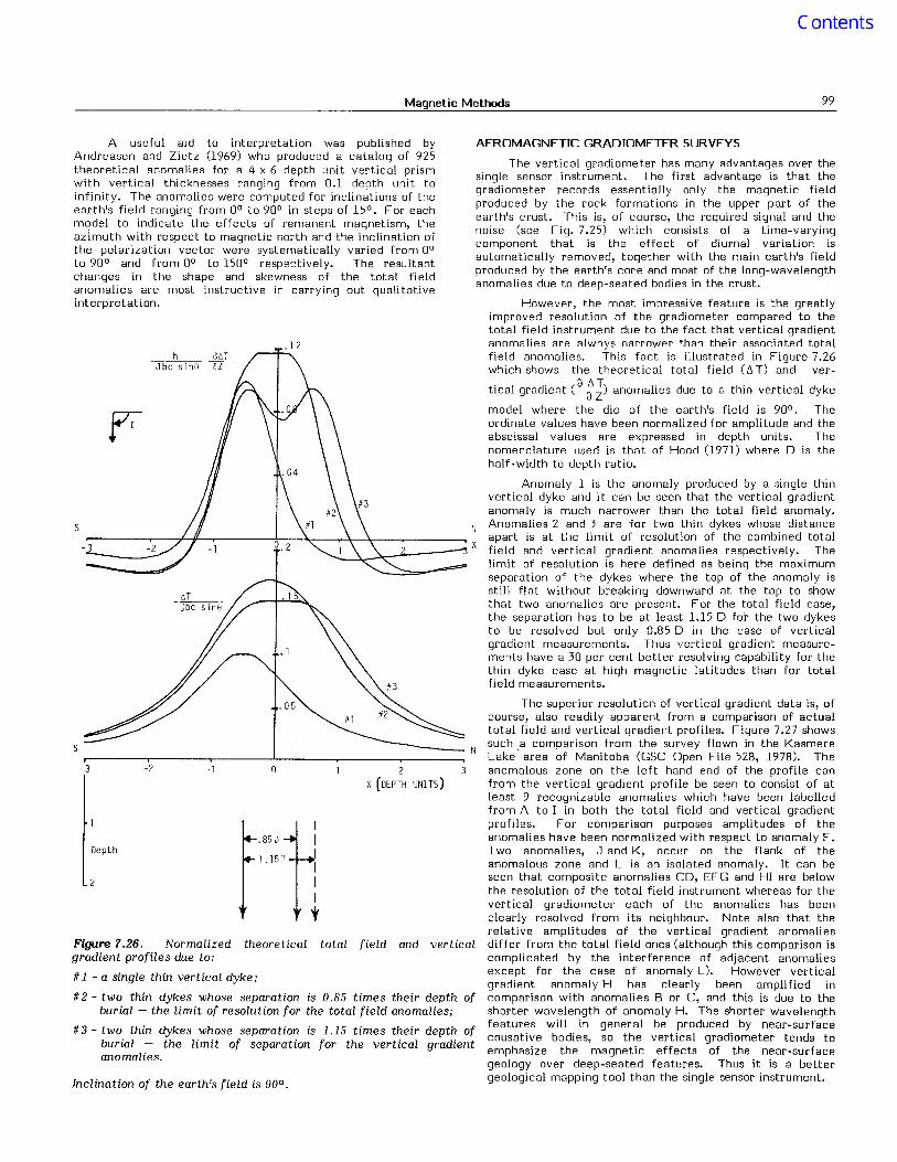
Magnetic Methods 99

AEROMAGNETIC GRADIOMETER SURVEYS

Jbc sinS

The vertical gradiometer has many advantages over thesingle sensor instrument. The first advantage is that thegradiometer records essentially only the magnetic fieldproduced by the rock formations in the upper part of theearth's crust. This is, of course, the required signal and thenoise (see Fig. 7.25) which consists of a time-varyingcomponent that is the effect of diurnal variation isautomatically removed, together with the main earth's fieldproduced by the earth's core and most of the long-wavelengthanomalies due to deep-seated bodies in the crust.

However, the most impressive feature is the greatlyimproved resolution of the gradiometer compared to thetotal field instrument due to the fact that vertical gradientanomalies are always narrower than their associated totalfield anomalies. This fact is illustrated in Figure 7.26which shows the theoretical total field (!:i T) and ver-

tical gradient (a ~i) anomalies due to a thin vertical dyke

model where the dip of the earth's field is 90 0 • Theordinate values have been normalized for amplitude and theabscissal values are expressed in depth units. Thenomenclature used is that of Hood (1971) where 0 is thehalf-width to depth ratio.

Anomaly 1 is the anomaly produced by a single thinvertical dyke and it can be seen that the vertical gradientanomaly is much narrower than the total field anomaly.

rl Anomalies 2 and 3 are for two thin dykes whose distance~----"T--:;hf--.-------k-::--~----.-\--"":~-~----... apart is at t:le limit of resolution of the combined total

~_~~.,-J-_---JX field and vertical gradient anomalies respectively. Thelimit of resolution is here defined as being the maximumseparation of the dykes where the top of the anomaly isstill flat without breaking downward at the top to showthat two anomalies are present. For the total field case,the separation has to be at least 1.15 0 for the two dykesto be resolved but only 0.850 in the case of verticalgradient measurements. Thus vertical gradient measure­ments have a 30 per cent better resolving capability for thethin dyke case at high magnetic latitudes than for totalfield measurements.

A useful aid to interpretation was published byAndreasen and Zietz (1969) who produced a catalog of 925theoretical anomalies for a 4 x 6 depth unit vertical prismwith vertical thicknesses ranging from 0.1 depth unit toinfinity. The anomalies were computed for inclinations of theearth's field ranging from 00 to 900 in steps of 150. For eachmodel to indicate the effects of remanent magnetism, theazimuth with respect to magnetic north and the inclination ofthe polarization vector were systematically varied from 00to 900 and from 00 to 1500 respectively. The resultantchanges in the shape and skewness of the total fieldanomalies are most instructive in carrying out qualitativeinterpretation.

-3 -2 -1 o 2X (DEPTH UNITS)

Depth.85 D

Figure 7.26. Normalized theoretical total field and verticalgradient profiles due to:

#1 - a single thin vertical dyke;

#2 - two thin dykes whose separation is 0.85 times their depth ofburial - the limit of resolution for the total field anomalies;

# 3 - two thin dykes whose separation is 1.15 times their depth ofburial - the limit of separation for the vertical gradientanomalies.

Inclination of the earth's field is 90 0 •

100 Peter J. Hood et aI.

NW·

L

J

K

2000 m'

J'"o~

62'J53.38

Be~T

y0

w Cl w 0

• :::J '0- 0........ -lIOO:

~a:a:~w~

1:" > o..J >:c "'--'2 '"a: a: wo ,0 ....- raJ "'_a: a:::: a: (I)

DOW...Jcr ~--' >WDWWD~'" :::J-"- /I • ...J "-

w:r:a: /I.-J...JU>...Ja:a:z wt-7U-a:roO(/)'I-a::f-X(f)cr:--J

60150.09

l..070 lO~ER BOOM

15·35 F

b~TH

bZx2·06 yIm

g A

>0,"'~

1.74

8070 OftROIENr

Figure 7.27. Aeromagnetic profiles demonstrating the superior resolution of vertical gradientover total field data. Kasmere Lake. Manitoba (eSC Open File 528, 1978).

In Figures 25.2 and 25.3 of Paper 25 of this volume,Coope and Davidson (1979) have presented the verticalgradient and total field maps of a survey flown over theWhite Lake granite pluton in southeastern Ontario.Figure 25.1 in the same paper is part of GSC geologicalmap 1046A (Quinn, 1952) covering the survey area. Theairborne results were also issued as Open File Report 339 bythe Geological Survey of Canada (Hood et al., 1976). It isreadily apparent from a comparison of the maps that agreater amount of geological information of a more precisenature may be derived from vertical gradient maps. Forinstance, the two diabase dykes that cut the granite plutonare much narrower on the vertical gradient map. It should benoted in those maps that there is evidence of zoning withinthe granite pluton itself in the vertical gradient map andseveral fault zones are evident. In fact, fault zones are muchmore readily apparent on vertical gradient than on total fieldmaps. Thus vertical gradient aeromagnetic surveys wouldappear to be of particular value in porphyry copperexploration programs. It should however be pointed out thata somewhat closer flight line spacing must be used inaeromagnetic gradiometer surveys because of the higherresolution of the technique in order to avoid coherencyproblems. We conclude that vertical gradient aeromagneticsurveys are a viable alternative to total or vertical fieldground magnetic surveys.

Another important property of vertical gradient data isits abili ty to delineate geological contacts becausePrecambrian Shield areas usually consist of rock formationsof relatively large areal extent separated from one anotherby steeply dipping contacts. Figure 7.28 shows the resultantvertical gradient (solid line) and total field (dashed line)curves over a wide elongated rock formation with slopingsides which is located at a high magnetic latitude such asCanada. For this particular geometric mode:, actually adyke, the half width to depth ratio is 5. For comparisonpurposes, the amplitude of the two curves has been madeapproximately equal. It can be seen that there are two cross­overs from positive to negative values for the verticalgradient profile with the zero gradient values occurring closeto either of the contacts. In contrast, the total field anomalyis much less definitive in delineating the edges of thecausative rock formation. Actually if the dip of the earth'sfield and the contacts were vertical, then the zero gradientvalue would accurately coincide with the position of thecontact. However, it can be shown mathematically that the ,line joining the maximum and minimum gradient valuescrosses the vertical gradient profile itself at the point wherethe contact is located. This important property has beenillustrated in Figure 7.28. Thus on vertical gradientaeromagnetic maps flown at high magnetic latitudes, the zerogradient contours will delineate the contacts of major rockformations having some measurable magnetization contrastwith adjacent formations in a reasonably accurate fashion.

Magnetic Methods 101

zero

thetool

--

-1·5

Figure 7.28. Vertical gradient and total field profiles over a widedipping dyke; inclination of the earth's magnetic field = 75°.

It follows therefore that vertical gradient aeromagneticsurvey results8l'e in fact a better tool for geological mappingprograms than the more conventional total field results.Moreover, because many orebodies are located at or nearcontacts, the vertical gradient technique should proveinvaluable in tracing such contacts using airborne techniques.

There is a great deal of aeromagnetic survey dataavailable throughout the world and it is possible to derive thefirst vertical gradient data from the total field results.Although there is some loss of accuracy when compared withthe measured vertical gradient data (Hood et al., 1976),nevertheless the resultant end product reflects the underlyinggeology much better than the total field map. McGrath et a1.(1976) has devised a compilation procedure for the purposewhich uses a two-dimensional vertical gradient operator(McGrath, 1975). It is necessary, however, that the totalfield data be of high quality without significant levellingerrors because these tend to be emphasized in the resultantmap.

Thus to summarize, the main advar;1tages ofaeromagnetic gradiometer as a geological mappingcompared to the single sensor (total field) technique are:

direct delineation of vertical contacts by thegradient contour value, i.e. vertical contact mapper;

superior resolution of anomalies produced by closely­spaced geological formations;

anomalies produced by near-surface features areemphasized with respect to those resulting from moredeeply-buried rock formations; and

regional gradient of the earth's magnetic field and diurnalvariation are automatically removed.

REGIONAL MAGNETIC ANOMALY MAPS

Recognition of the value of regional magneticcompilations has grown appreciably in the last decade sincethe first magnetic anomaly map of Canada, and probably thefirst such map of its kind in the world, was presented at the1967 symposium in Niagara Falls by Morley et a1. (1968). Athird edition of the Magnetic Anomaly Map of Canada waspublished by the Geological Survey of Canada (McGrathet aI., 1977) in time for the Exploration 77 Symposium. Themap was derived from approximately 8250 1:63 360 total­field aeromagnetic maps and was published at the scale of1:5 000 000 using a colour contour interval of 200 y. Seamagnetometer data were also included. For the compilation,

the main geomagnetic field which has its origin in theearth's core was subtracted from the map data by agraphical separation technique (McGrath et aI., 1978).Thus the residual magnetic features shown in this map arerelated mainly to sources within the crust of the earth.Because of the small scale of the map, magnetic featuresless than 8 km wide do not show up. Hence the map canbe regarded as reflecting large-scale near-surface andmajor deep-seated crustal features. The main uses of amap of this type are threefold. Firstly, as an index map itpresents an overview of the aeromagnetic survey coverageof Canada. Secondly, the map presents the major patternsproduced by the continental rocks in the Canadianlandmass and may be used both as an aid in theinterpretation of regional geological features in thebasement rocks as well as to help in the planning of moredetailed investigations. Lastly and probably the mostimportant use of the map is as a vehicle or medium toinitially stimulate comparisons of magnetic features withother types of geoscientific compilations.

Plate 1 shows part of the area extending from JamesBay on the east to the Province of Manitoba on the westfrom the Magnetic Anomaly Map of Canada. The large

magnetic high areas (red) correlate well with terrainunderlain by rocks of granitic composition. Also there is anobvious correspondence between greenstone belts and theirmetamorphic equivalents with the broad magnetic low areas(green). For example, the Wabigoon volcanic belt (WB) isassociated with a magnetic low. Thus it is within the broadmagnetic low areas in which most of the economic oredeposits occur. Locally magnetic highs in greenstone beltsare associated with iron formation, iron-rich tholeiitic basaltsand iron-rich basic intrusive rocks. Volcanic rocks of calc­alkaline and komatiitic affinities are generally nonmagnetic.

The continuity of the magnetic patterns over largeareas is particularly evident and contrast with the variationin the patterns from one area to another. Some of themagnetic anomaly pattern changes occur at geologicalprovince boundaries. For example, the trace of the changefrom the predominantly east-west trending anomalies in themagnetic high area over northwestern Ontario as compared tothe magnetic low northeast-southwest trends to thenorthwest in Manitoba delineates the edge of the Churchill­Superior province (CSB).

Other pattern changes occur within a given geologicalprovince. The Kapuskasing Lineament (KL) extending fromJames Bay to the eastern end of Lake Superior is a structuralzone within a geological province in which both the magneticbase level and the magnetic anomaly patterns change. On theother hand, the Quetico structural zone (QS) is associatedwith a linear magnetic low which transgresses through themagnetic anomaly pattern associated with the westernSuperior province.

It seems apparent from the examples presented in theforegoing discussion that in general a great deal ofcorrelation exists between the magnetic and geologiccompilations and that the production of such nationalmagnetic anomaly maps is worthwhile and should beencouraged by other nations.

A number of interesting regional magnetic studies havebeen carried out by workers in various countries and amongthe more interesting are those by McGrath and Hall, 1969;Hall and Oagley, 1970; Kornik, 1971; Zietz et al., 1971;Krutikhovskaya et al., 1973; Hood and Tyl, 1977.

International Geomagnetic Reference Field

As aeromagnetic coverage of large continental areaswas completed during the early sixties and the results were

102 Peter J. Hood et at.

Am, K.1972:

compiled into regional magnetic anomaly maps, the need toeliminate the dominating effect of the earth's main fieldbecame apparent. In a country such as Canada the earth'smagnetic field varies by an amount of 7000 y or so in goingfrom the east and west coasts to the centre of the country.The amplitude of anomalies due to crustal rocks exceptin the case of magnetic iron formation is less than1000 y. Consequently if the main field which is due to themagnetic properties of the earth's core were not removed,the resultant map would be dominated by a series of parallelcontours due to the main earth's field and there is aconsequent distortion of the crustal anomalies e.g. the peaksare displaced. If the main earth's field is removed, it ispossible to produce a coloured map utilizing four or fivecolours each representing a 200 y contour interval torepresent the crustal magnetic field. Accordingly amathematical model of the main earth's field called theInternational Geomagnetic Reference Field (IGRF 1965.0)was adopted at the Symposium on the Description of theEarth's Magnetic Field held in Washington from October 22­25, 1968. The 1965.0 IGRF was defined by a set of sphericalharmonic coefficients to degree and order 8, which requires80 coefficients, and a linear secular variation correction wasincorporated (F abiano and Peddie, 1969; Cain and Cain, 1971).It has transpired that the secular variation corrections chosenwere not particularly accurate and this has resulted in errorsof the IGRF of up to a few hundred gammas in fi ve years(Regan and Cain, 1975). At the Grenoble Assembly of theIUGG in 1975 it was resolved that IGRF 1965.0 be replaced byIGRF 1975.0 to be used until at least 1980. This new modelconsists of IGRF 1965.0 brought up to epoch 1975.0 for itsmain field coefficients plus new coefficients for secularchange (Barraclough and Fabiano, 1977). It is hoped that withthe launching of U.S. magnetic field satellite (Magsat) inSeptember 1979, that an analysis of the resultant data willresult in a more accurate mathematical model of the earth'smagnetic field (Cain, 1971; Langel et al., 1977).

SUMMARY AND CONCLUSIONS

During the past decade both ground and airbornemagnetometers have been improved considerably byminiaturization and made more reliable by the extensive useof integrated circuit devices. Digital-recording ofaeromagnetic survey data is now standard procedure andexcept for the flight recovery process, the compilation ofaeromagnetic maps is now a completely automated process.The resultant gridded data generated for the machinecontouring process also facilitate the production of a varietyof derived and processed maps to any scale or map projectionfor use in the subsequent interpretation of the aeromagneticdata. Aeromagnetic gradiometry has also been proven to be auseful tool in the mapping of Precambrian terrane.

Quantitative interpretation methods have seennoticeable advances during the past decade particularly thoseusing the computer to match observed and calculatedanomalies by a best-fit process.

Thus after more than a quarter century theaeromagnetic survey technique is still being improved inmany new and novel ways and it remains the most utilizedairborne survey technique in terms of the line kilometrageflown each year throughout the world. This continuedpopularity is due in part to a variety of reasons. Of all theairborne geophysical survey techniques, the aeromagneticmethod has by far the greatest depth penetration being ableto detect features down to the Curie point geotherm some20 km or so beneath the earth's surface. Moreover in contrastto other airborne techniques, the aeromagnetic method isunaffected by the presence of surficial material such asoverburden and tropical weathering or by the presence oflakes and swamps. Aeromagnetic surveys also provide a

continuity of information at low cost that is impossible toachieve in ground geophysical or geological surveys, and oneof the outstanding advantages of aeromagnetic surveysbecomes apparent when large areas are surveyed becauselarge regional geological features are often discovered.These may not be recognizable on the ground because theyare so large or are perhaps obscured by sedimentaryformations. Clearly further significant developments in theaeromagnetic survey technique can be expected in the nextdecade especially in the application of digital recording andprocessing techniques.

REFERENCES

The arbitrarily magnetized dyke: interpretationby characteristics; Geophys. Explor., v. 10 (2),p. 63-90.

Andreasen, G.E. and Zietz, I.1969: Magnetic fields for a 4 x 6 prismatic model; U.S.

Geol. Surv., Prof. Paper 666, 219 p.

Barraclough, D.R. and Fabiano, E.B.1977: Grid values and charts for the IGRF 1975.0; Int.

Assoc. Geomag. Aeron., Bull. 38, 134 p.

Bott, M.H.P. and Hutton, M.A.1970: A matrix method for interpreting oceanic

magnetic anomalies; Geophys. J. v. 20 (2),p. 149 157.

Cain, J.C.1971: Geomagnetic models from satellite surveys; Rev.

Geophys. Space Phys., v. 9, p. 259-273.

Cain, J.C. and Cain, S.J.1971: Derivation of the International Geomagnetic

Reference Field; NASA, Tech. Note D-6237(IGRF 10/68).

Collin, C.R., Salvi, A., Lemercier, D., Lemercier, P., andRobach, F.

1973: Magnetometre differentiel a haute sensibilite;Geophys. Prosp., v. 21 (4), p. 704-715.

Coope, J.A. and Davidson, M.J.1979: Some aspects of integrated exploration; in

Geophysics and Geochemistry in the Search forMetallic Ores, Geol. Surv. Can., Econ. Geol.Rep. 31, Paper 25.

Dutton, D.H. and Nisen, W.G.1978: The expanding realm of computer cartography;

Datamation, p. 134-142, June 1978.

Fabiano, E.B. and Peddie, N.W.1969: Grid values of total magnetic intensity IGRF­

1965; U.S. Env. Sci. Servo Admin., Tech. Rept. 38,55 p.

Geological Survey of Canada1978: Aeromagnetic gradiometer survey, Kasmere Lake

area, Manitoba; Geol. Surv. Can., Open File 528.

Goree, W.S. and Fuller, M.1976: Magnetometers using RF-driven Squids and their

applications in rock magnetism andpaleomagnetism; Rev. Geophys. Space Phys., V. 14(4), p. 591-608.

Grant, F.S.1972: Review of data processing and interpretation

methods in gravity and magnetics, 1964-1971;Geophysics, v. 37 (4), p. 647-661-

1974: Timmins magnetic susceptibility map; Geol. Surv.Can., Open File 229.

Magnetic Methods 103

on(4),

determination of depthprofiles; Geophysics, v. 36

Naudy, H.1971: Automatic

aeromagneticp.717-722.

O'Brien, D.P.

Lantto, V.1973: Characteristic curves for interpretation of highly

magnetic anomalies in borehole measurements;Geoexpl., v. 11 (2), p. 75-85.

McGrath, P .H.1975: A two-dimensional first vertical derivative

operator; in Report of Activities, Part A, Geol.Surv. Can.;-Paper 75-1A, p. 107-108.

McGrath, P.H., Haley, E.L., Reveler,D.A., andLetourneau, C.P.

1978: Compilation techniques employed in constructingthe Magnetic Anomaly Map of Canada; in CurrentResearch, Part A, Geol. Surv. Can., Paper 78-1A,p. 509-515.

McGrath, P.H. and Hall, D.H.1969: Crustal structure in northwestern Ontario:

regional magnetic anomalies; Can. J. Earth Sci.,v. 6 (1), p. 101-107.

McGrath, P.H. and Hood, P.J.1970: The dipping dike case: a computer curve-

matching method of magnetic interpretation;Geophysics, v. 35 (5), p. 831-848.

1973: An automatic least-squares multi-model methodfor magnetic interpretation; Geophysics, v. 38 (2),p. 349-358.

McGrath, P.H., Hood, P.J., and Darnley, A.G.1977: Magnetic anomaly map of Canada; Geol. Surv.

Can., Map 1255A C3rd Ed.).

McGrath, P.H., Kornik, L.J., and Dods, 5.D.1976: A method for the compilation of high quality

calculated first vertical derivative aeromagneticmaps; in Report of Activities, Part C, Geol. Surv.Can., Paper 76-1C, p. 9-17.

Morley, L.W., MacLaren, A.S., and Charbonneau, B.W.1968: Magnetic anomaly map of Canada; Geo!. Surv.

Can., Map 1255A (lst Ed.).

1970: Two-dimensional inverse convolution filters foranalysis of magnetic field; 40th Ann. Int. Meet.,Soc. Explor. Geophys., New Orleans (Abstr.).

1971: An automated method for magnetic anomalyresolution and depth-to-source computation; Proc.Symp. on Treatment and Interpretation ofAeromagnetic Data, Berkeley, California.

1972: Compudepth: a new method for depth-to-basement computation; 42nd Ann. Mtg., Soc.Explor. Geophys., Anaheim, California (Preprint).

Koulomzine, T., Lamontagne, Y., and Nadeau, A.1970: New methods for the direct interpretation of

magnetic anomalies caused by inclined dikes ofinfinite length; Geophysics, v. 35 (5), p. 812-830.

Krutikhovskaya, Z.A., Pashkevich, I.K., and Simonenko, T.N.1973: Magnetic anomalies of Precambrian Shields and

some problems of their geological interpretation;Can. J. Earth Sci., v. 10 (5), p. 629-636.

Langel, R.A., Regan, R.D., and Murphy, J.P.1977: Magsat: a satellite for measuring near earth

magnetic fields; Goddard Space Flight Center,Rep. X-922-77-199.

geomagnetism; Trans. 2ndInt. Assoc. Geomag.

Japan, 1973, Bull. 35,

1971:

1972:

1977:

1976:

1973:

1978:

Hood, P.1970:

Hahn, A.1978: Die Einheiten des internationalen Systems in der

Geomagnetik; J. Geophys., v. 44, p. 189-202.

Hall, D.H. and Dagley, P.1970: Regional magnetic anomalies: an analysis of the

smoothed aeromagnetic map of Great Britain andNorthern Ireland; Inst. Geo!. Sci., UK, Rep. 70/10,8 p.

Hartman, R.R., Teskey, D.J., and Friedberg, J.L.1971: A system for rapid digital aeromagnetic

interpretation; Geophys., v. 36 (5), p. 891-918.

Holroyd, M. T.1974: The aeromagnetic data automatic mapping

(ADAM) system; in Report of Activities, Part B,Geo!. Surv. Can., Paper 74-1B, p. 79-82.

Holroyd, M. T. and Bhattacharyya, B.K.1970: Automatic contouring of geophysical data using

bicubic spline interpolation; Geol. Surv. Can.,Paper 70-55,40 p.

IAGA1973:

Magnetic surveying instrumentation; a review ofrecent advances; in Mining and GroundwaterCeophysics 1967 (L-:W. Morley, Ed.), Geol. Surv.Can., Econ. Geo!. Rep. 26, p. 3-3I.

Geophysical applications of high resolutionmagnetometers; in Encyclopedia of Physics,Springer-Verlag, Berlin, v. 49 (3), p. 422-460.

Mineral exploration: trends and developments in1972; Can. Min. J., v. 93 (2), p. 175-199.

Mineral exploration: trends and developments in1972; Can. Min. J., v. 94 (2), p. 167-182.

Mineral exploration: trends and developments in1975; Can. Min. J., v. 97 (2), p. 163-197.

Mineral exploration: trends and developments in1976; Can. Min. J., v. 98 (1), p. 8-47.

Mineral exploration: trends and developments in1977; Can. Min. J., v. 99 (1), p. 8-53.

Hood, P., Sawatzky, P., Kornik, L.J., and McGrath, P.H.1976: Aeromagnetic gradiometer survey, White Lake,

Ontnrio; Geol. Surv. Can., Open File 339.

Hood, P. and Tyl, I.1977: Residual magnetic anomaly map of Guyana and its

regional geological interpretation; Mem. SecondLatin Amer. Cong., Caracas, v. 3, p. 2219-2235.

Hood, P. and Ward, S.H.1969: Airborne geophysical methods; in Advances in

Geophysics, Academic Press, New York, v. 13,p. 1-112.

Adoption of 51 units inGen. Sci. Assembly,Aeronomy, Kyoto,p. 148 15I.

Johnson, W. W.1969: A least-squares method of interpreting magnetic

anomalies caused by two-dimensional structures;Geophysics, v. 34 (1), p. 65-74.

Kornik, L.J.1971: Magnetic subdivision of Precambrian rocks in

Manitoba; Geol. Assoc. Can., Spec. Paper 9,p. 51 60.

104 Peter J. Hood et aI.

Ogawa, K. and Tsu, H.1976: Magnetic interpretation using interactive

computer graphics; Japan Pet. Dev. Corp., Tech.Res. Center, Rep. 3, p. 19-39.

Quinn, H.A.1952: Renfrew map area, Renfrew and Lanark Counties,

Ontario; Geo!. Surv. Can., Paper 51-27, 79 p.

Rao, B.S.R., Murthy, 1.V.R., and Rao, C.V.1973: Two methods for computer interpretation of

magnetic anomalies of dikes; Geophysics, v. 38(4), p. 710-718.

Regan, R.D. and Cain, J.C.1975: The use of geomagnetic field models in magnetic

surveys; Geophysics, v. 40 (4), p. 621-629.

Sarwinski, R.E.1977: Superconducting instruments; Cryogenics,

p. 671 679, Dec.

Sawatzky, P. and Hood, P.J.1975: Fabrication of an inboard digital-recording

vertical gradiometer system for aeromagneticsurveying: a progress report; in Report ofActivities, Part A, Geo!. Surv. Can.-;-Paper 75-1A,p. 139-140.

Otala, M.1969: The theory and construction of a proposed

superconducting aeromagnetic gradiometer; ActaPolytech. Scand., Helsinki, Elect. Eng. Ser. 21,55 p.

Spector, A. and Grant, F .5.1970: Statistical models for interpreting aeromagnetic

data; Geophysics, v. 35 (2), p. 293-302.

Spector, A. and Parker, W.1979: Computer compilation and interpretation of

geophysical data; in Geophysics and Geochemistryin the Search for Metallic Ores, Geol. Surv. Can.,Econ. Geol. Rep. 31, Paper 23.

Steenland, N.C.1970: Recent developments in aeromagnetic methods;

Geoexplor., v. 8 0/4), p. 185-204.

Zablocki, C.J.1974: Magnetite assays from magnetic susceptibility

measurements in taconite production blast holes;Geophysics, v. 39 (2), p. 174-189.

Zietz,1., Hearn, B.C., Higgins, M.W., Robinson, G.D., andSwanson, D.A.

1971: Interpretation of an aeromagnetic strip across thenorthwestern United States; Geo!. Soc. Am. Bull.,v. 82 (12), p. 3347-3372.