The Astrophysical Journal, 794:132 (12pp), 2014 October 20 doi:10.1088/0004-637X/794/2/132C⃝ 2014. The American Astronomical Society. All rights reserved. Printed in the U.S.A.

MAGNETIC EFFECTS IN HOT JUPITER ATMOSPHERES

T. M. Rogers and T. D. KomacekDepartment of Planetary Sciences, University of Arizona, Tucson, AZ 85721, USA; tami@lpl.arizona.edu

Received 2014 March 24; accepted 2014 August 22; published 2014 October 1

ABSTRACT

We present magnetohydrodynamic simulations of the atmospheres of hot Jupiters ranging in temperature from 1100to 1800 K. Magnetic effects are negligible in atmospheres with temperatures !1400 K. At higher temperatureswinds are variable and, in many cases, mean equatorial flows can become westward, opposite to their hydrodynamiccounterparts. Ohmic dissipation peaks at temperatures ∼1500–1600 K, depending on field strength, with maximumvalues ∼1018 W at 10 bars, substantially lower than previous estimates. Based on the limited parameter study done,this value cannot be increased substantially with increasing winds, higher temperatures, higher field strengths,different boundary conditions, or lower diffusivities. Although not resolved in these simulations, there is modestevidence that a magnetic buoyancy instability may proceed in hot atmospheres.

Key words: hydrodynamics – magnetohydrodynamics (MHD)

1. INTRODUCTION

Exoplanet research is an expeditiously changing field, drivenby the discovery of more than 1450 exoplanets to date. Asmany of these exoplanets are discovered by either the radialvelocity or transit technique, there is a natural bias towarddiscovering planets that both have large radii and are close totheir host star. These close-in extrasolar giant planets, or “hotJupiters,” are nominally assumed to be tidally locked to theirhost star and have strong atmospheric flows driven by theirhigh irradiation, 103–106 times the flux that Jupiter receives.This results in the unique atmospheric dynamics of these hotJupiters, with equatorial superrotation and strong day–nightflow predicted to occur from purely hydrodynamical numericalsimulations (Cho et al. 2003; Showman & Guillot 2002; Cooper& Showman 2005; Dobbs-Dixon & Lin 2008; Showman et al.2009; Rauscher & Menou 2010; Lewis et al. 2010; Thrastarson& Cho 2010; Heng et al. 2011; Mayne et al. 2014). Thesesimulations also predict eastward displacement of the hot spotfrom the substellar point, first predicted by Showman & Guillot(2002) and confirmed through observations of HD 189733bby Knutson et al. (2007, 2012). However, the extremely hightemperatures present in many hot Jupiter atmospheres point tohigh levels of ionization, which could lead to magnetic effects,which we discuss in this work.

The combination of radial velocity data, transit light curves,and spectrometry has enabled observations to place strongconstraints on the mass, radius, composition, temperature, andwind structure of hot Jupiters, leading them to be the most wellcharacterized planets outside our solar system. However, thereare still many unexplained observations, such as the extremevariability of the dayside–nightside circulation efficiency ofthese planets (Cowan & Agol 2011) and the larger-than-expected radii of many hot Jupiters (Bodenheimer et al. 2001,2003; Guillot & Showman 2002; Baraffe et al. 2003; Laughlinet al. 2005). The circulation efficiency of extrasolar giantplanet (EGPs) is determined by combining information frominfrared and visible phase curves, with some planets (e.g.,HD 209458b, HD 189733b) having very efficient circulationfrom dayside to nightside and hence small (<500 K) zonal(east–west) temperature variations (Cowan et al. 2007; Knutsonet al. 2007), and some (e.g., Ups And b, WASP-12b) having

weak circulation and large day–night temperature variations(Crossfield et al. 2010; Cowan et al. 2012). Using a statisticalapproach of 24 transiting exoplanets with light curves, Cowan& Agol (2011) conclude that hot Jupiters show a variety ofrecirculation efficiencies, with no clear trend with temperature.However, they do note that the hottest planets in their samplehave the lowest recirculation efficiencies, with a fairly sharptransition at Teff ≈ 2400 K. Reduced circulation efficienciesmight be expected at high temperatures where magnetic fieldsare able to reduce wind speeds.

The enhanced radii of many hot Jupiters are likely solvedby invoking an additional heat source in the giant planetinterior to counteract their gravitational contraction. A varietyof heating mechanisms have been proposed, e.g., tidal heating(Bodenheimer et al. 2001, 2003; Jackson et al. 2008), depositionof energy from waves (Guillot & Showman 2002), forcedturbulence (Youdin & Mitchell 2010), and, most recently, ohmicdissipation (Batygin & Stevenson 2010; Perna et al. 2010b;Laughlin et al. 2011). The exact amount of heating necessary toinflate these hot Jupiters is uncertain, but it is approximately10−2 to 10−6 of the stellar incident flux, depending on thecomposition of the planet and the depth at which this energyis deposited (Bodenheimer et al. 2001; Showman & Guillot2002). Using 90 well-characterized EGPs, Laughlin et al. (2011)found that the radius anomaly (the difference between theobserved radius and predicted radius from evolutionary models,∆R = Robs − Rpred) is positively correlated with the effectivetemperature of the planet. This points toward ohmic dissipationas a viable mechanism, which is supported by recent models(Batygin & Stevenson 2010; Perna et al. 2010b; Wu & Lithwick2013). Though other heating mechanisms may explain a portionof the observed radii (Baraffe et al. 2003), Batygin et al. (2011)claim that only ohmic dissipation coupled with metallicityvariations can explain the entire spectrum of hot Jupiter radiusobservations.

Coupling the effects of magnetic drag (which reduces windspeeds) and ohmic dissipation, Menou (2012a) showed thatohmic dissipation has a peak temperature beyond which itdecays owing to the strong influence of the Lorentz forceslowing wind speeds past a critical equilibrium temperature.For a 10 G field, Menou (2012a) finds that ohmic dissipationpeaks at ∼1600 K, remarkably close to the peak seen in the

1

The Astrophysical Journal, 794:132 (12pp), 2014 October 20 Rogers & Komacek

Laughlin et al. (2011) data for radius anomaly, adding furtherconfidence that ohmic dissipation is the explanation for inflatedhot Jupiter radii. However, more recently the viability of ohmicdissipation as the heating mechanism has been questioned.Adding the scaling laws of Menou (2012a) to a one-dimensional(1D) planetary evolution model, Huang & Cumming (2012)found ohmic dissipation to be too weak to explain the radii ofhot Jupiters with masses "0.4 MJup. Using a similar radiative-convective model but including the effects of nightside cooling(making the model 1+1D), Spiegel & Burrows (2013) foundthat ohmic dissipation cannot by itself produce a runaway inplanet radius as predicted by Batygin et al. (2011). Additionally,the recent general circulation models (GCMs) of HD 209458band HD 189733b by Rauscher & Menou (2013), using akinematic model for wind drag and a parameterization of ohmicdissipation, could not explain the inflated radii of those planetsfor dipole magnetic field strengths !10 G without assuming alarge interior heat flux and extrapolating using scalings fromWu & Lithwick (2013).

In the first self-consistent magnetohydrodynamic (MHD)simulations of a hot Jupiter atmosphere that included ohmic dis-sipation, Rogers & Showman (2014) showed that ohmic dissipa-tion fell short of explaining the inflated radius of HD 209458bby nearly two orders of magnitude. This is in stark contrastwith the results of Batygin & Stevenson (2010), Batygin et al.(2011) and Perna et al. (2010b), who find that the ohmic dissipa-tion at depth can explain, and even overpredict, the radii of thepopulation of hot Jupiters. However, the models of Batygin &Stevenson (2010) and Batygin et al. (2011) assumed that a fixedamount of the incident stellar flux went into ohmic dissipation,and Perna et al. (2010b) did not include feedback from magneticdrag in their GCMs. As a result of the variety of methodologiesused to explore ohmic dissipation and the extreme sensitivity ofeach model to parameters that vary from planet to planet, thereare large discrepancies in the literature on magnetic effects inhot Jupiter atmospheres and interiors.

Currently, many of the unexplained observations of hot EGPatmospheres have been attributed to planetary magnetic fields.However, only two self-consistent MHD models of the in-teraction of planetary magnetic fields with atmospheric dy-namics have been conducted (Batygin et al. 2013; Rogers &Showman 2014), and only one (Rogers & Showman 2014) in-cludes ohmic dissipation. Such models are necessary if thesetheories are to be made robust. Here we extend the workof Rogers & Showman (2014) to cover a range of atmo-spheric temperatures (and hence magnetic diffusivities) to un-derstand the breadth of possible magnetic effects in hot Jupiteratmospheres.

2. NUMERICAL METHODS

We use a three-dimensional (3D), MHD model in the anelasticapproximation. The model is based on the Glatzmaier dynamocode (Glatzmaier 1984, 1985) but has substantial differencesin the actual equations solved, the discretization, and theimplementation. A description of the axisymmetric version ofthis code can be found in Rogers (2011). The model solves thefollowing equations:

∇ · ρv = 0 (1)

∇ · B = 0 (2)

ρ =

⎡

⎣(

∂ρ

∂T

)

p

T +

(∂ρ

∂p

)

T

p

⎤

⎦ (3)

ρ∂v∂t

= − ∇ · (ρvv) − ∇p − ρgr (4)

+ 2ρv × ! + ∇ · (2ρν(eij − 13

(∇ · v)δij ))

+1µ0

(∇ × B) × B

∂B∂t

= ∇ × (v × B) − ∇ × (η∇ × B) (5)

∂T

∂t+ (v · ∇)T

= −vr

(∂T

∂r− (γ − 1)T hρ

)

+ (γ − 1)T hρvr

+ γ κ

[∇2T + (hρ + hκ )

∂T

∂r

]

+Teq − T

τrad+

η

µoρcp

|∇ × B|2. (6)

Equation (1) represents the continuity equation in the anelas-tic approximation (Ogura & Phillips 1962; Gough 1969;Glatzmaier 1984; Rogers & Glatzmaier 2005), where ρ is thereference state density and v is the gas velocity. The anelasticapproximation was developed for dealing with convection andwinds in Earth’s atmosphere and therefore does not fully cap-ture the large atmospheric wind velocities likely on hot Jupiters.While not ideal, the progress obtained by performing full MHDmodels (as opposed to the kinematic models previously exe-cuted) vastly outweighs the inaccuracy associated with slightlylower wind speeds.1 Equation (2) represents the conservationof magnetic flux, and Equation (3) is the equation of state,which we take here to be an ideal gas. The momentum equa-tion, including Coriolis and Lorentz forces, is represented byEquation (4), where p represents pressure, ! is the angular ve-locity of the rotating frame of reference, eij is the rate of straintensor, ν is the viscous diffusivity, and B is the magnetic field.

The magnetic induction equation is represented byEquation (5), where η is the magnetic diffusivity (see be-low for treatment of the magnetic diffusivity). The energyEquation (6) is written here as a temperature equation withT the reference state temperature, κ the thermal diffusivity, andhρ , hκ representing inverse density and thermal diffusivity scaleheights, respectively. We note that the thermal and viscous dif-fusivities in Equations (4) and (6) can be functions of radius.The first term on the right-hand side (rhs) of Equation (6) rep-resents the super- or subadiabaticity of the region and thereforeallows us to treat both convective and stably stratified regions,which is unnecessary in this work but may be necessary in thefuture. The fourth term on the rhs of Equation (6) represents the

1 Note that this form of the anelastic equations does not conserve energy forlinear perturbations (Durran 1989). In order to test whether this had an effectin the flows described here, we implemented the fix suggested by Brown et al.(2012) in our hydrodynamic models. After 1200 Prot we find that the flows arequalitatively virtually identical. Quantitatively, the energy-conservingformalism suggested in Brown et al. (2012) leads to maximum flow speeds thatare slightly larger (5%).

2

The Astrophysical Journal, 794:132 (12pp), 2014 October 20 Rogers & Komacek

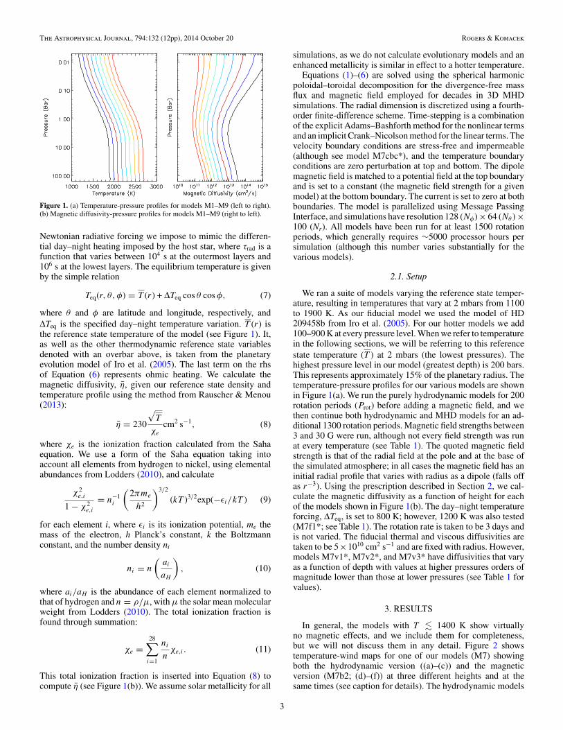
Figure 1. (a) Temperature-pressure profiles for models M1–M9 (left to right).(b) Magnetic diffusivity-pressure profiles for models M1–M9 (right to left).

Newtonian radiative forcing we impose to mimic the differen-tial day–night heating imposed by the host star, where τrad is afunction that varies between 104 s at the outermost layers and106 s at the lowest layers. The equilibrium temperature is givenby the simple relation

Teq(r, θ,φ) = T (r) + ∆Teq cos θ cos φ, (7)

where θ and φ are latitude and longitude, respectively, and∆Teq is the specified day–night temperature variation. T (r) isthe reference state temperature of the model (see Figure 1). It,as well as the other thermodynamic reference state variablesdenoted with an overbar above, is taken from the planetaryevolution model of Iro et al. (2005). The last term on the rhsof Equation (6) represents ohmic heating. We calculate themagnetic diffusivity, η, given our reference state density andtemperature profile using the method from Rauscher & Menou(2013):

η = 230

√T

χe

cm2 s−1, (8)

where χe is the ionization fraction calculated from the Sahaequation. We use a form of the Saha equation taking intoaccount all elements from hydrogen to nickel, using elementalabundances from Lodders (2010), and calculate

χ2e,i

1 − χ2e,i

= n−1i

(2πme

h2

)3/2

(kT )3/2exp(−ϵi/kT ) (9)

for each element i, where ϵi is its ionization potential, me themass of the electron, h Planck’s constant, k the Boltzmannconstant, and the number density ni

ni = n

(ai

aH

), (10)

where ai/aH is the abundance of each element normalized tothat of hydrogen and n = ρ/µ, with µ the solar mean molecularweight from Lodders (2010). The total ionization fraction isfound through summation:

χe =28∑

i=1

ni

nχe,i . (11)

This total ionization fraction is inserted into Equation (8) tocompute η (see Figure 1(b)). We assume solar metallicity for all

simulations, as we do not calculate evolutionary models and anenhanced metallicity is similar in effect to a hotter temperature.

Equations (1)–(6) are solved using the spherical harmonicpoloidal–toroidal decomposition for the divergence-free massflux and magnetic field employed for decades in 3D MHDsimulations. The radial dimension is discretized using a fourth-order finite-difference scheme. Time-stepping is a combinationof the explicit Adams–Bashforth method for the nonlinear termsand an implicit Crank–Nicolson method for the linear terms. Thevelocity boundary conditions are stress-free and impermeable(although see model M7cbc*), and the temperature boundaryconditions are zero perturbation at top and bottom. The dipolemagnetic field is matched to a potential field at the top boundaryand is set to a constant (the magnetic field strength for a givenmodel) at the bottom boundary. The current is set to zero at bothboundaries. The model is parallelized using Message PassingInterface, and simulations have resolution 128 (Nφ) × 64 (Nθ ) ×100 (Nr). All models have been run for at least 1500 rotationperiods, which generally requires ∼5000 processor hours persimulation (although this number varies substantially for thevarious models).

2.1. Setup

We ran a suite of models varying the reference state temper-ature, resulting in temperatures that vary at 2 mbars from 1100to 1900 K. As our fiducial model we used the model of HD209458b from Iro et al. (2005). For our hotter models we add100–900 K at every pressure level. When we refer to temperaturein the following sections, we will be referring to this referencestate temperature (T ) at 2 mbars (the lowest pressures). Thehighest pressure level in our model (greatest depth) is 200 bars.This represents approximately 15% of the planetary radius. Thetemperature-pressure profiles for our various models are shownin Figure 1(a). We run the purely hydrodynamic models for 200rotation periods (Prot) before adding a magnetic field, and wethen continue both hydrodynamic and MHD models for an ad-ditional 1300 rotation periods. Magnetic field strengths between3 and 30 G were run, although not every field strength was runat every temperature (see Table 1). The quoted magnetic fieldstrength is that of the radial field at the pole and at the base ofthe simulated atmosphere; in all cases the magnetic field has aninitial radial profile that varies with radius as a dipole (falls offas r−3). Using the prescription described in Section 2, we cal-culate the magnetic diffusivity as a function of height for eachof the models shown in Figure 1(b). The day–night temperatureforcing, ∆Teq, is set to 800 K; however, 1200 K was also tested(M7f1*; see Table 1). The rotation rate is taken to be 3 days andis not varied. The fiducial thermal and viscous diffusivities aretaken to be 5×1010 cm2 s−1 and are fixed with radius. However,models M7v1*, M7v2*, and M7v3* have diffusivities that varyas a function of depth with values at higher pressures orders ofmagnitude lower than those at lower pressures (see Table 1 forvalues).

3. RESULTS

In general, the models with T ! 1400 K show virtuallyno magnetic effects, and we include them for completeness,but we will not discuss them in any detail. Figure 2 showstemperature-wind maps for one of our models (M7) showingboth the hydrodynamic version ((a)–(c)) and the magneticversion (M7b2; (d)–(f)) at three different heights and at thesame times (see caption for details). The hydrodynamic models

3

The Astrophysical Journal, 794:132 (12pp), 2014 October 20 Rogers & Komacek

Table 1Model Parameters

Model T Bo ν κ η ∆Teq τmag Bφm OD WS EFF

M1 1100 0 5. 5. NA 800 NA NA NA 2.8 NAM1b1 1100 10 5. 5. 1260. 800 2.06 d9 0.78 0.12 2.8 3.6M1b2 1100 30 5. 5. 1260. 800 2.37 d8 2.3 1.0 2.8 30.3M2 1200 0 5. 5. NA 800 NA NA NA 2.9 NAM2b1 1200 10 5. 5. 580. 800 1.03 d8 2.2 0.33 2.9 10.0M2b2 1200 30 5. 5. 580. 800 1.4 d7 6.0 3.0 2.9 90.9M3 1300 0 5. 5. NA 800 NA NA NA 3.0 NAM3b1 1300 10 5. 5. 360. 800 3.6 d6 7.2 0.63 3.0 19.1M3b2 1300 30 5. 5. 360. 800 4.66 d5 20.1 4.8 3.0 145.5M4 1400 0 5. 5. NA 800 NA NA NA 3.1 NAM4b1 1400 10 5. 5. 150. 800 2.9 d5 18.6 3.7 3.1 112.1M4b2 1400 30 5. 5. 150. 800 5.0 d4 44.6 21.0 3.5 636.4M5 1500 0 5. 5. NA 800 NA NA NA 3.1 NAM5b1 1500 10 5. 5. 84. 800 2.1 d4 48.5 13. 3.3 393.9M5b2 1500 30 5. 5. 84. 800 7.5 d3 81.3 28. 2.9 848.5M5b3 1500 3 5. 5. 84. 800 2.0 d5 15.8 1.3 3.1 3.4M6 1600 0 5. 5. NA 800 NA NA NA 3.2 NAM6b1 1600 10 5. 5. 48. 800 2.1 d3 111. 26. 2.6 787.9M6b2 1600 30 5. 5. 48. 800 1.26 d3 144. 25. 2.2 757.6M6b3 1600 3 5. 5. 48. 800 1.05 d4 49.8 5.2 3.2 157.6M7 1700 0 5. 5. NA 800 NA NA NA 3.2 NAM7b1 1700 10 5. 5. 29. 800 263.8 234.5 20. 2.3 606.1M7b2 1700 30 5. 5. 29. 800 317. 213.9 22. 2.0 666.7M7b3 1700 3 5. 5. 29. 800 995.8 120.7 13. 3.0 393.9M7v1 1700 0 0.5 0.5 NA 800 NA NA NA 2.7 NAM7v1b1 1700 10 0.5 0.5 29. 800 320. 212.9 30.6 2.2 927.3M7v2 1700 0 0.05 0.05 NA 800 NA NA NA 2.9 NAM7v2b1 1700 10 0.05 0.05 29. 800 404.8 189.3 36. 2.0 1090.9M7v3 1700 0 0.02 0.02 NA 800 NA NA NA 2.9 NAM7v3b1 1700 10 0.02 0.02 29. 800 417. 186.5 38.5 2.5 1166.7M7f1 1700 0 5. 5. NA 1200 NA NA NA 3.6 NAM7f1b1 1700 10 5. 5. 29. 1200 228.4 239. 29. 2.6 878.8M7f1b2 1700 30 5. 5. 29. 1200 253.9 252. 30. 2.4 909.1M7cbc 1700 0 5. 5. NA 800 NA NA NA 2.3 NAM7cbcb1 1700 10 5. 5. 29. 800 335.3 208. 17. 1.5 515.2M8 1800 0 5. 5. NA 800 NA NA NA 2.9 NAM8b2 1800 10 5. 5. 18. 800 215.7 208.9 12. 2.3 363.6M8b3 1800 3 5. 5. 18. 800 195.7 199.0 23. 3.0 670.0M9 1900 0 5. 5. NA 800 NA NA NA 2.9 NAM9b3 1900 3 5. 5. 12. 800 69.1 278.2 17.5 3.2 530.3

Notes. T is the temperature of the reference state model, T , at 2 mbar in K; see Figure 1. Bo is the model field strength; “0” indicates ahydrodynamic model, whereas other values are in gauss and represent the radial field at the pole, at the bottom of the domain. Viscous (ν),thermal (κ), and magnetic (η) diffusivities are in units of 1010 cm2 s−1 and are values at 10 bars. ∆Teq is the day–night forcing described inEquation (7). The magnetic timescale is in seconds and is calculated using the maximum toroidal field strength, Bφm at 1500 Prot, and themagnetic diffusivity at 0.5 bars (the region where the toroidal field strength peaks). OD is the ohmic dissipation integrated below 10 bars in1018 W, and WS is the peak wind speed at 1500 Prot in km s−1. EFF is the efficiency of conversion from incident stellar flux to ohmic dissipationin parts per million.

show behavior similar to previous models of hot Jupiter winds:a chevron-like pattern that leads to predominantly eastwardflow at the equator. Weak westward flows are seen high inthe atmosphere and at some longitudes, but eastward flow isdominant at the equator. The hot spot is displaced eastward ofthe substellar point (which is at 0◦ longitude). Meridional flow ispoleward westward of the hot spot and equatorward eastward ofthe hotspot. There are also a couple of discrepancies comparedwith previous models. First, despite predominantly eastwardflow near the equator (and eastward flow on zonal average), wedo see some longitudes that show westward flow. Second, thetemperature structure at depth with cool equator and hot poles(Figure 2(c)) is opposite to that previously found. Both thesemay be due to the use of explicit thermal diffusivities, whichchanges slightly the overall thermal forcing.

Comparing the hydrodynamic flows to the magnetic models,we note several differences: (1) the magnetic model is hotteroverall, (2) the magnetic model shows smaller day–night tem-perature differences, (3) the magnetic model has predominantlywestward flow, (4) the magnetic model has weaker meridionalflow, and (5) the magnetic model is asymmetric about the equa-tor. We will address many of these differences in the followingsections.

3.1. Magnetic Field Evolution

For cooler models, the imposed field is virtually unaffectedby the flow, and there is no field evolution, virtually no inducedtoroidal field or current, and hence little Lorentz force and littleohmic dissipation. This can be seen in the top row of Figure 3,

4

The Astrophysical Journal, 794:132 (12pp), 2014 October 20 Rogers & Komacek

Latit

ude

Longitude Longitude

MHDHD(a)

(b)

(c)

(d)

(e)

(f)

Figure 2. Temperature perturbation (K), shown in color, and winds, shown with arrows as a function of longitude and latitude, for models M7 ((a)–(c)) and M7b2((d)–(f)) at 10 mbars ((a) and (d)), 70 mbars ((b) and (e)), and 10 bars ((c) and (f)).

which shows the evolution of magnetic field in models M2b2.There we see that the initially imposed dipole field is barelydistorted. For hot planets in which the field is sufficiently tied tothe flow, field lines are swept toward the nightside of the planetby winds flowing away from the substellar point (both eastwardand westward). Because eastward flow is favored, toroidal fieldinduction is predominantly positive in the northern hemisphere(NH) and negative in the southern hemisphere (SH) near theequator. Since the winds are dragged by the Lorentz force andthe field is swept both eastward and westward, the field is notcontinually wrapped around the circumference of the planet.Rather, fields of opposite signs meet on the nightside of theplanet, causing toroidal field strengths and currents to peakthere. The resulting large gradients in the toroidal field causestrong variation in the Lorentz force and unsteady flow and field,particularly for stronger fields and/or higher temperatures (notereversals in the bottom row of Figure 3). This leads to variabilityand asymmetry in the zonal flows and hence variability in hot-spot displacement; see Section 3.4.

In hotter models the induced toroidal field strength growsrapidly and peaks around 0.1–0.2 bars, as seen in Figure 4,where zonal wind shear is strong (see Figure 11). One can seethat the peak field amplitude grows in time and that the magneticlayer spreads. With maximum wind speeds of ∼km s−1, theequipartition field strength is of order 100–200 G dependingon the depth of the flow (density). In the hot models, toroidalfield strengths easily reach values in excess of this (Figure 4 andTable 1). Stated another way, the Alfven speed (vA = B/

√4πρ)

is as large as, or larger than, the peak wind speed.2The stability of the field to buoyancy instability is deter-

mined not only by the field strength but also by its radialstructure, the stabilizing effect of gravity (the Brunt–Vaisalafrequency, N), and the diffusion coefficients (thermal, viscous,and magnetic) (Silvers et al. 2009). In these models the Richard-son number, N2/(dU/dz)2, is approximately ∼10, so winds are

2 The magnetic pressure at these field strengths is equivalent to ∼1 mbar.

hydrodynamically stable. For hot, magnetic models the ideal(nondiffusive) instability criterion outlined in Acheson (1978)is satisfied at some times and in some locations and becomesmore frequent the hotter the model. However, diffusive effectsare likely very important in these models. For example, Silverset al. (2009) showed that if η < κ , then buoyancy instability isenhanced by double diffusive effects. Models just slightly hotterthan those presented would have η < κ , and we note that wewere not able to run such models with magnetic fields (hotterhydrodynamic models are possible) as an instability (of un-known nature) always developed. Further, the short timescalesassociated with Newtonian cooling at the surface are physicallyequivalent to much larger values of κ . For example, a coolingtime of 104 s is something like a κ of 1014 cm2 s−1, resultingin η ≪ κ , again possibly enhancing buoyancy instability in hotmodels. The resolution in these models is insufficient to capturea buoyancy instability if one were to develop. However, giventhe arguments above, a buoyancy instability appears probablein the hottest atmospheres. Turbulence arising from such aninstability may provide a downward flux of heat that could con-tribute to planetary radius inflation, as suggested by Youdin &Mitchell (2010). Therefore, more work should be done investi-gating buoyancy instability under these hot Jupiter conditions.

Because the magnetic diffusivity is not a function of all space,we are not able to investigate the instability proposed by Menou(2012b). However, it is possible that differential ohmic heatingaffects dynamics. Ohmic heating causes the temperature to risethroughout the atmosphere. However, because the current isstrongest on the nightside, ohmic heating is stronger there,causing the nightside to heat up more than the dayside, therebyreducing day–night temperature differences and hence reducingatmospheric forcing (see Figure 5). In the models presented here,this effect is relatively small and may not persist if the magneticdiffusivity were a function of all space. In that case, atmosphericflow-field coupling may be reduced on the nightside, whichcould lower the current (and hence ohmic heating). On the otherhand, the magnetic diffusivity would be locally higher, which

5

The Astrophysical Journal, 794:132 (12pp), 2014 October 20 Rogers & Komacek

Figure 3. Magnetic field evolution. The viewpoint is looking onto the nightside of the planet. Top row shows field lines for M2b2, with color representing the toroidalfield magnitude, with red/magenta positive (with maximum of 5 G), blue negative (with minimum of −5 G), and yellow representing values between ±1 G. Middleand bottom rows show field lines for M7f1b1 and M7f1b2, respectively. Again, color represents toroidal field strength, with red/magenta positive with maximum of260 G, blue negative with minimum −260 G, and yellow representing field strengths in the range ±20 G. Times are different for each model and are meant only togive a qualitative picture of magnetic field evolution.

Figure 4. Time evolution of horizontally averaged toroidal field as a function ofdepth for models M7b1 (solid lines) and M7b2 (dotted lines). Induced toroidalfield peaks around 0.1–0.2 bars, where vertical shear is large. The field strengthincreases with time starting at 330 Prot and increasing in increments of ∼115 Protto 1500 Prot.

Figure 5. Day–night temperature differential as a function of pressure. Thesolid line is the hydrodynamic version, dotted lines are 10 G MHD models,and dashed lines are 30 G MHD models. Red lines represent cool models, M2,M2b1, and M2b2, and black lines represent hot models, M7, M7b1, and M7b2.

6

The Astrophysical Journal, 794:132 (12pp), 2014 October 20 Rogers & Komacek

Figure 6. (a) Zonal-mean zonal winds at two heights (10 mbars, higher speeds,and 2 bars, lower speeds), averaged near the equator as a function of temperature.Black squares represent hydrodynamic models, cyan triangles represent 10 Gfield, red diamonds represent 30 G field, and blue asterisks represent 3 G fieldstrength. (b) Ohmic dissipation (W) at 10 bars as a function of temperature,shown with the same symbols.

would increase ohmic heating, and it is unclear how these twoeffects would interact. We will be addressing this in future work.

3.2. Magnetic Scaling Laws

Menou (2012a) developed scaling laws for magnetic effectscoupling both the effects of wind drag and ohmic dissipation. Heshowed that as the temperature of an atmosphere is increased,field-flow coupling is enhanced and a magnetic field can morereadily slow wind speeds, which, in turn, will reduce ohmicdissipation. His theory predicted a temperature at which ohmicdissipation peaks and furthermore predicted an anticorrelationbetween displacement of the hot spot on a planetary surfaceand the radius anomaly. With our suite of models we can testthose predictions in the context of this more complete model.In Figure 6 we show (a) zonal-mean zonal wind speeds as afunction of temperature at two different pressure levels (2 barsand 10 mbars) and (b) ohmic dissipation at 10 bars. The mostobvious result is that the overall behavior produced in our self-consistent MHD models is remarkably similar to that predictedby (Menou 2012a, see his Figures 1 and 3): magnetic effects havelittle effect on slowing cooler atmospheres, but wind speeds dropprecipitously above 1400–1500 K, and ohmic dissipation dropsabove 1500–1600 K, with larger field strengths peaking at lowertemperatures.

There are, however, a few interesting and important differ-ences. First, with respect to ohmic dissipation, the amplitudeof the ohmic heating is two to three orders of magnitude lowerthan that predicted by previous authors (Batygin & Stevenson2010; Batygin et al. 2011; Menou 2012a). Second, with regardto the magnetic effects on winds, hotter models show zonal-mean zonal winds that reverse sign and become retrograde (orwestward). That is, the effect of magnetic fields is not simply toslow the flow, but can act to change the overall structure of theflow (see Figure 2). These differences will be addressed in thenext sections.

3.3. Ohmic Dissipation

There are several reasons that the ohmic dissipation is lowerin these self-consistent simulations than previously predicted;most are physical limitations of the reduced equations employed

in previous attempts to include magnetic effects (Batygin &Stevenson 2010; Perna et al. 2010a, 2010b; Rauscher & Menou2013), and one may be a limitation of our anelastic model.

The first step in estimating ohmic dissipation in manyprevious models is estimating the current using a reduced formof Ohm’s law,

J = 14πη

((v × B) + E) ≈ 14πη

(v × B) , (12)

neglecting the electric field. Retaining only the latitudinalcurrent and assuming that the radial velocity is sufficiently small,the current is approximated as

Jθ = 14πη

(vrBφ − vφBr ) ≈ −vφBr

4πη. (13)

Using this current, the ohmic dissipation and Lorentz force canbe estimated:

P = 4πηJ2 ≈v2

φB2r

4πη, (14)

J × B ≈ −vφB2r

4πη. (15)

The validity of the first step in this estimate, calculating thecurrent, can be tested by comparing Equation (13) with thelatitudinal current calculated from Ampere’s law J = ∇ ×B/µ;this comparison is shown in Figure 7. For the approximation,we use velocities taken from this simulation and a constantmagnetic field strength, as has been done previously (Perna et al.2010a; Rauscher & Menou 2013). One can see there that theapproximation overestimates the peak current (note amplitudeson color bar) by two orders of magnitude and does not accuratelyreflect the spatial distribution of the current. This overestimatecarries over to the ohmic dissipation, where the approximation(shown in Figures 8(b) and (d)) overestimates the peak ohmicdissipation ((a) and (c)) by two to four orders of magnitudeand again fails to account for the spatial distribution. Uponintegration in radius, this leads to ohmic dissipation rates thatare generally two to three orders of magnitude smaller thanestimates using the prescription outlined in Equations (12)–(15)above (values at 10 bars can be seen in Figure 6, and integratedvalues can be seen in Table 1).

The inconsistency between our models and previous estimatesstems from neglecting the electric field in Ohms law, whichis only valid in the limit that ∂B/∂t is small. This is alsoequivalent to assuming the low magnetic Reynolds number limit(Rm ! 1). With horizontal flow speeds of order 105 cm s−1,length scales of order 109 cm, and magnetic diffusivities asseen in Figure 1(b), our hottest models have Rm of 100–1000,clearly in violation of the approximation. One can also see inFigures 3 and 4 that magnetic field evolution is substantial, andneglecting this evolution leads to large discrepancies betweenour self-consistent model and previous estimates.

Considering a rather hot model of HD 209458b with aninterior temperature of 2500 K leads to ∼1018 W of ohmicheating at 10 bars. There are many estimates for the amountof heating required to inflate the radius. Showman & Guillot(2002) state that 10% of stellar insolation is required at 5 bars,1% at 100 bars, and 0.08% if the energy is deposited atthe center. Batygin et al. (2011) find that 1%–3% of stellar

7

The Astrophysical Journal, 794:132 (12pp), 2014 October 20 Rogers & Komacek

Figure 7. Comparison of current calculated using the approximation encapsu-lated in Equations (13)–(15) (b, d, labeled “Prescription”) and current calculatedfrom Ampere’s law (a, c, labeled “Current”) at 0.5 bars (a, b) and at 100 bars(c, d); units are G cm−1. One can see that the spatial distribution is not wellrepresented by the approximation and, more importantly, the amplitude recov-ered using the approximation is two orders of magnitude larger than the actualcurrent.

insolation integrated throughout the planet is required. For astellar insolation of 3.3 × 1022 W, we find an efficiency ofconversion from incident stellar flux to ohmic dissipation (i.e.,the ratio of integrated ohmic dissipation to incident stellar flux)of 0.006% for the most favorable case with 2.2 × 1019 W ofdissipation integrated below 10 bars; see Table 1. Batygin &Stevenson (2010) require 4 × 1018 W in the convective interiorto inflate the radius for a solar-metallicity, no-core model ofHD 209458b. For HD 209458b 1% of stellar insolation wouldrequire ∼1020 W, so our peak atmospheric heating of ∼1018 Wwould appear too weak to explain the inflated radius by twoorders of magnitude. We can extrapolate our heating in the windzone of the planet to interior regions as in Rauscher & Menou(2013) by using the scalings of Wu & Lithwick (2013), assumingconservation of currents between the atmosphere and interior.To order-of-magnitude precision, Wu & Lithwick (2013) predictthat the ohmic dissipation in the interior (below the bottomboundary of our model) is a factor of ∼ zwind/Rp lower than thatin the atmosphere. The thickness of our modeled atmosphere,from 2 mbars to 200 bars, is ∼1.2 × 109 cm (about 14% of thestellar radius). Hence, given an integrated atmospheric ohmicheating of 1 × 1018 W, we expect a total ohmic heating ratebelow the bottom boundary of 1.4 × 1017 W. This estimate ismore than an order of magnitude below the necessary 4×1018 Winterior dissipation from Batygin & Stevenson (2010). Morerealistic models for HD 209458b, in terms of temperature,appear too weak by up to three orders of magnitude (1300 Ksurface temperature, 2000 K interior temperature, 10 G field).The effects of various parameters, as well as the possibility thatour lower wind speeds contribute to this shortcoming, will bediscussed in Section 3.5.

(a)

(b)

(c)

(d)

Figure 8. Comparison of ohmic dissipation calculated using Equation (14) (b, d,labeled “Prescription”) compared to that calculated in simulation (a, c, labeled“ohmic Dissipation”); units are W cm−2. In Equation (14) we use velocitiesfrom this simulation and a constant magnetic field strength of 30 G.

3.4. Zonal Winds

Previous work implementing the Lorentz force in GCMsof the atmospheres of hot Jupiters (e.g., Perna et al. 2010a;Rauscher & Menou 2013) did so by incorporating a Rayleighdrag, similar to the implementation of Schneider & Liu (2009)previously for Jupiter itself. This kinematic method slows thezonal wind through adding a drag term = −u/τmag to the zonalcomponent momentum equation, where the magnetic timescaleτmag (or the inverse relaxation coefficient for Rayleigh drag) isdefined as τmag = 4πρη/B2 (Rauscher & Menou 2013). ForJupiter, Schneider & Liu (2009) find that a reduced heat fluxcombined with strong drag can inhibit superrotation and intro-duce retrograde flow (subrotation). However, no previous workon hot Jupiter atmospheres has found this effect. Similar to thediscussion above, in treating the Lorentz force simply as a dragon the zonal component of the momentum equation, one mustneglect the evolution of the magnetic field because the Lorentzforce only acts like a drag on the fluid velocity perpendicularto the magnetic field. Therefore, one must assume a pure dipolein order to assume that the zonal flow is continuously perpen-dicular to it. As can be seen in Figure 3, this is not a goodassumption, particularly for hot models (high Rm).

Here we find that the effect of magnetic fields on zonal windscan be treated as drag only in a narrow range of temperatures,where Rm is low. At higher temperatures (higher Rm), theeffect of magnetic fields is not simply to act as drag. At thelowest temperatures the magnetic field has virtually no effecton the wind speeds or geometry; the magnetic diffusivity issufficiently high that the magnetic flow just slips past themagnetic field unimpeded. At 1400–1600 K, depending onthe field strength, the magnetic field starts to slow the windin the upper and lower atmosphere. For higher temperatures,and at larger field strengths, the zonal–mean zonal wind reverses

8

The Astrophysical Journal, 794:132 (12pp), 2014 October 20 Rogers & Komacek

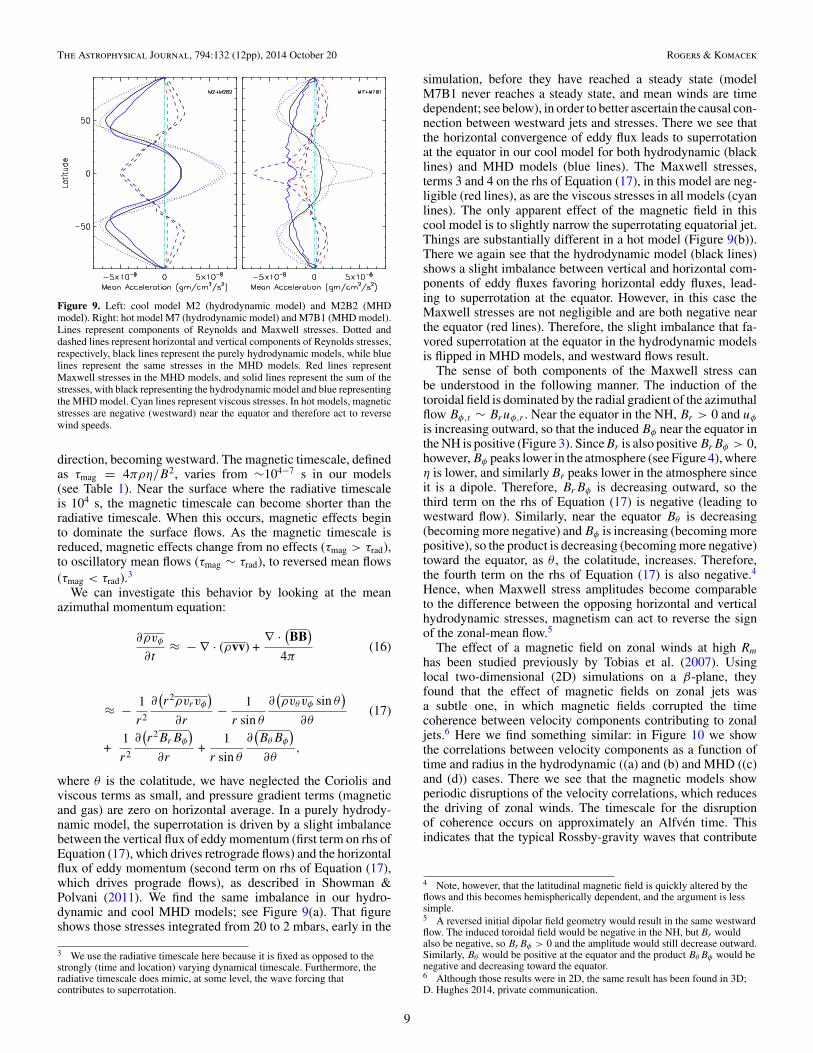
Figure 9. Left: cool model M2 (hydrodynamic model) and M2B2 (MHDmodel). Right: hot model M7 (hydrodynamic model) and M7B1 (MHD model).Lines represent components of Reynolds and Maxwell stresses. Dotted anddashed lines represent horizontal and vertical components of Reynolds stresses,respectively, black lines represent the purely hydrodynamic models, while bluelines represent the same stresses in the MHD models. Red lines representMaxwell stresses in the MHD models, and solid lines represent the sum of thestresses, with black representing the hydrodynamic model and blue representingthe MHD model. Cyan lines represent viscous stresses. In hot models, magneticstresses are negative (westward) near the equator and therefore act to reversewind speeds.

direction, becoming westward. The magnetic timescale, definedas τmag = 4πρη/B2, varies from ∼104−7 s in our models(see Table 1). Near the surface where the radiative timescaleis 104 s, the magnetic timescale can become shorter than theradiative timescale. When this occurs, magnetic effects beginto dominate the surface flows. As the magnetic timescale isreduced, magnetic effects change from no effects (τmag > τrad),to oscillatory mean flows (τmag ∼ τrad), to reversed mean flows(τmag < τrad).3

We can investigate this behavior by looking at the meanazimuthal momentum equation:

∂ρvφ

∂t≈ − ∇ · (ρvv) +

∇ ·(BB

)

4π(16)

≈ − 1r2

∂(r2ρvrvφ

)

∂r− 1

r sin θ

∂(ρvθvφ sin θ

)

∂θ(17)

+1r2

∂(r2BrBφ

)

∂r+

1r sin θ

∂(BθBφ

)

∂θ,

where θ is the colatitude, we have neglected the Coriolis andviscous terms as small, and pressure gradient terms (magneticand gas) are zero on horizontal average. In a purely hydrody-namic model, the superrotation is driven by a slight imbalancebetween the vertical flux of eddy momentum (first term on rhs ofEquation (17), which drives retrograde flows) and the horizontalflux of eddy momentum (second term on rhs of Equation (17),which drives prograde flows), as described in Showman &Polvani (2011). We find the same imbalance in our hydro-dynamic and cool MHD models; see Figure 9(a). That figureshows those stresses integrated from 20 to 2 mbars, early in the

3 We use the radiative timescale here because it is fixed as opposed to thestrongly (time and location) varying dynamical timescale. Furthermore, theradiative timescale does mimic, at some level, the wave forcing thatcontributes to superrotation.

simulation, before they have reached a steady state (modelM7B1 never reaches a steady state, and mean winds are timedependent; see below), in order to better ascertain the causal con-nection between westward jets and stresses. There we see thatthe horizontal convergence of eddy flux leads to superrotationat the equator in our cool model for both hydrodynamic (blacklines) and MHD models (blue lines). The Maxwell stresses,terms 3 and 4 on the rhs of Equation (17), in this model are neg-ligible (red lines), as are the viscous stresses in all models (cyanlines). The only apparent effect of the magnetic field in thiscool model is to slightly narrow the superrotating equatorial jet.Things are substantially different in a hot model (Figure 9(b)).There we again see that the hydrodynamic model (black lines)shows a slight imbalance between vertical and horizontal com-ponents of eddy fluxes favoring horizontal eddy fluxes, lead-ing to superrotation at the equator. However, in this case theMaxwell stresses are not negligible and are both negative nearthe equator (red lines). Therefore, the slight imbalance that fa-vored superrotation at the equator in the hydrodynamic modelsis flipped in MHD models, and westward flows result.

The sense of both components of the Maxwell stress canbe understood in the following manner. The induction of thetoroidal field is dominated by the radial gradient of the azimuthalflow Bφ,t ∼ Bruφ,r . Near the equator in the NH, Br > 0 and uφ

is increasing outward, so that the induced Bφ near the equator inthe NH is positive (Figure 3). Since Br is also positive BrBφ > 0,however, Bφ peaks lower in the atmosphere (see Figure 4), whereη is lower, and similarly Br peaks lower in the atmosphere sinceit is a dipole. Therefore, BrBφ is decreasing outward, so thethird term on the rhs of Equation (17) is negative (leading towestward flow). Similarly, near the equator Bθ is decreasing(becoming more negative) and Bφ is increasing (becoming morepositive), so the product is decreasing (becoming more negative)toward the equator, as θ , the colatitude, increases. Therefore,the fourth term on the rhs of Equation (17) is also negative.4Hence, when Maxwell stress amplitudes become comparableto the difference between the opposing horizontal and verticalhydrodynamic stresses, magnetism can act to reverse the signof the zonal-mean flow.5

The effect of a magnetic field on zonal winds at high Rmhas been studied previously by Tobias et al. (2007). Usinglocal two-dimensional (2D) simulations on a β-plane, theyfound that the effect of magnetic fields on zonal jets wasa subtle one, in which magnetic fields corrupted the timecoherence between velocity components contributing to zonaljets.6 Here we find something similar: in Figure 10 we showthe correlations between velocity components as a function oftime and radius in the hydrodynamic ((a) and (b) and MHD ((c)and (d)) cases. There we see that the magnetic models showperiodic disruptions of the velocity correlations, which reducesthe driving of zonal winds. The timescale for the disruptionof coherence occurs on approximately an Alfven time. Thisindicates that the typical Rossby-gravity waves that contribute

4 Note, however, that the latitudinal magnetic field is quickly altered by theflows and this becomes hemispherically dependent, and the argument is lesssimple.5 A reversed initial dipolar field geometry would result in the same westwardflow. The induced toroidal field would be negative in the NH, but Br wouldalso be negative, so BrBφ > 0 and the amplitude would still decrease outward.Similarly, Bθ would be positive at the equator and the product BθBφ would benegative and decreasing toward the equator.6 Although those results were in 2D, the same result has been found in 3D;D. Hughes 2014, private communication.

9

The Astrophysical Journal, 794:132 (12pp), 2014 October 20 Rogers & Komacek

vθvφhvrvφh

vrvφm vθvφm

(a) (b)

(c) (d)

Figure 10. Reynolds stresses contributing to zonal flow in hydrodynamic models (a,b, model M7) and MHD models (c, d, model M7b1) at the equator as a function oftime and pressure in the atmosphere. One can see that the velocity fluctuations are anticorrelated and steady in time in the hydrodynamic models, but this correlationis intermittently disrupted with opposite correlations in the MHD cases. This results in variability of the equatorial zonal wind.

to the eastward zonal jet are additionally influenced by Alfvenwaves in the high Rm limit.

Despite these effects, the reversed and severely dragged meanzonal winds are limited to the upper layers of the atmosphere(pressure levels below 0.1 bars, where the Rm is largest), whileat deeper levels (where Rm is small) the winds are merelydragged; see Figure 11. This results in a reduction of the hot-spotdisplacement eastward of the substellar point. Figure 12 showsthe hot-spot displacement at 60 mbars (a nominal depth forthe photosphere), as a function of temperature and magneticfield strength. Vertical lines on some data points indicate

the variability of the hot-spot displacement over 100Prot. Forhydrodynamic models (shown with plus signs), the hot-spotdisplacement increases with temperature from ∼35◦ to 60◦.If one considers reasonable field strengths (3 and 10 G), hot-spot displacement is affected significantly only at temperatureslarger than 1500 K, where it is reduced by as much as 20◦

but can vary by ∼10◦. Large observed hot-spot displacementstherefore imply either negligible magnetic field strength or lowsurface temperatures. High surface temperatures with large hot-spot displacements could therefore provide an upper limit onmagnetic field strength. Notably, the hot-spot displacement has

10

The Astrophysical Journal, 794:132 (12pp), 2014 October 20 Rogers & Komacek

Figure 11. Zonal-mean zonal wind, averaged over low latitudes, as a functionof pressure. Black lines represent model M7, blue lines represent M8, and redlines represent M6, with solid lines hydrodynamic models, dashed lines 10 Gmodels, and dotted lines 30 G models.

Figure 12. Hot-spot displacement as a function of temperature. Black plus signsdenote hydrodynamic models, blue diamonds represent 3 G magnetic models,cyan triangles represent 10 G models, and red squares represent 30 G models.Vertical lines represent the range over which the hot-spot displacement variesin 100Prot.

been measured on HD 209458b to be ∼40◦ (Zellem et al. 2014),consistent with our hydrodynamic and weak (!3 G) field results,which have negligible ohmic dissipation.7

7 Consistent with the reversed and oscillating winds higher in theatmosphere, the hot spot varies more wildly aloft, by as much as 30◦, and issometimes displaced westward of the substellar point.

Figure 13. (a) Zonal-mean zonal wind speeds in hydrodynamic models M7,M7v1, M7v2, M7v3, M7cbc, and M7f1 (vφh) vs. zonal-mean zonal wind speedsin their MHD counterparts M7b1, M7v1b1, M7v2b1, M7v3b1, M7cbcb1, andM7f1b1 (vφm). A 20 times increase in hydrodynamic model wind speeds resultsin only a 5 times increase in MHD model wind speeds. (b) Zonal-mean zonalwind speeds in the same hydrodynamic models as in (a) vs. ohmic dissipationin those models at 10 bars. A 20 times increase in hydrodynamic model windspeeds results in only a 2 times increase in ohmic dissipation.

3.5. Dependencies

Besides temperature and magnetic field strength, we investi-gated the effect of lowered diffusivities (viscous and thermal,M7v1*, M7v2*, M7v3*), velocity boundary conditions (no slipinstead of stress free, M7cbc*), and increased forcing (1200 Kinstead of 800 K, M7f1*), all at the same reference tempera-ture (1700 K) and field strength (10 G). Lowered diffusivitiesat depth and larger forcing lead to faster wind speeds at depthand increased ohmic dissipation. No-slip boundary conditionslead to reduced wind speeds and hence lower ohmic dissipa-tion. Figure 13(a) shows the zonal-mean zonal wind speeds inhydrodynamic models (vφh) versus the zonal-mean zonal windspeeds in their MHD counterparts (vφm). There we see thata 20 times increase in hydrodynamic wind speeds results inonly a 5 times increase in MHD wind speeds. Furthermore, this5 times increase in MHD wind speed results in only a 2 timesincrease in ohmic dissipation (Figure 13(b)). Therefore, it ap-pears that (1) the simple prescription in which ohmic dissipationis proportional to zonal wind speed squared is not an accuraterepresentation and (2) increased wind speeds are unlikely to beable to close the (large) gap between the ohmic dissipation cal-culated and the values typically considered necessary to explainthe inflated radii of massive hot Jupiters.

4. DISCUSSION

We have shown the basic effects of magnetism in the at-mospheres of hot Jupiters for a range of temperatures. At lowtemperatures, ionization is sufficiently low that the flow simplyslips past magnetic field lines unaffected. Around 1400–1500 K,the behavior changes. Temperatures are large enough to allowsufficient ionization for field-flow coupling and magnetic ef-fects, such as magnetic tension, magnetic pressure, and ohmicdissipation, to become relevant. This qualitative result has beenfound previously by Menou (2012a). We find that, even at itspeak, ohmic dissipation is substantially smaller than previouslycalculated and generally at least an order of magnitude lowerthan the requisite heating required to explain many hot Jupiterradii. We find that increasing wind speeds, changing boundaryconditions, increasing forcing, varying temperature, and varying

11

The Astrophysical Journal, 794:132 (12pp), 2014 October 20 Rogers & Komacek

field strength do not substantially alter this picture. However, toadequately evaluate whether ohmic dissipation is able to inflateindividual objects, it may be necessary to couple evolutionarymodels with the heating in a more sophisticated manner. It islikely that ohmic dissipation may be able to explain the radiiof lower-mass, inflated planets as found in Huang & Cumming(2012). Furthermore, since the most efficient heating (in termsof radius inflation) should occur deeper in the atmosphere, itmay be necessary to better resolve the dynamics of the deepatmosphere, where shallow, hydrostatic models are not optimal.

With regard to the magnetic effects on hot Jupiter windsand recirculation efficiency, we find a more complicated picturethan expected. As the magnetic timescale is progressivelydecreased (atmosphere becomes hotter and/or field becomesstronger), MHD effects progress from pure drag, to oscillatorymean flows, to stationary but westward mean flows. Therefore,high in the atmospheres of hot Jupiters with substantial fieldstrength, magnetic effects could cause the winds to vary on shorttimescales (timescales of an order of tens of rotation periods)and even cause mean flows and hot-spot displacements that arewestward. This leads to hot-spot displacements that are reducedcompared to their hydrodynamic counterparts and that can showsubstantial variability.

Additionally, we find that magnetic field evolution is morecomplicated than the simple kinematic picture. As temperaturesrise, magnetic diffusivity drops while induced fields and theirvertical gradients grow, resulting in more conducive conditionsfor magnetic buoyancy instability. Although we cannot resolvethe instability here, numerical instability coupled with favorableconditions indicates that such an instability may be possible inhot, magnetic atmospheres.

The models presented here have several shortcomings, whichshould be kept in mind when considering their results. First,these models are anelastic and hence preclude, at some level, thefast wind speeds commonly recovered in typical models of hotJupiter atmospheres. While this may have an effect on the degreeof ohmic heating, the winds at depths where ohmic dissipationis likely to be the most efficacious are highly uncertain. It isunclear at what level the dynamics of that region are drivenby the stellar insolation-driven winds aloft or the convectivemotions below, and more sophisticated models coupling thoseregions may be necessary to fully understand the dynamicsin that region and hence the ohmic dissipation there. Second,these models do not account for a fully time- and temperature-dependent magnetic diffusivity (which should be a functionof all space). While we doubt that this physics will have asubstantial effect on ohmic dissipation, it likely will affectthe wind structure, particularly high in the atmosphere, andit may affect the presence of instabilities that drive turbulence.We are working on including this effect, but we note that thelarge temperature variation (∼1000 K) seen in some planets islikely not computationally feasible, and similarly, extremely hotplanets will not be accessible without substantially increasedcomputational time and/or some extrapolation. Finally, ourreference state pressure-temperature profiles are rather crude,and more realistic profiles should be used in follow-up studies.This will be incorporated into future work looking at individualplanets.

With these caveats in mind, we have three main conclusions.1. Ohmic dissipation appears insufficient to explain all of the

inflated radii of observed hot Jupiters.2. Magnetic effects do not act simply to slow winds but

can have much more complicated, time-dependent effects,

which may be observable in phase curves (hot-spot dis-placement).

3. It appears probable, particularly in hot models, that amagnetic buoyancy instability could proceed, possiblyproducing turbulence in the atmosphere.

We are grateful to A. Cumming, G. Glatzmaier, D. Lin, A.Showman, and G. Vasil for helpful discussions. Support forthis research was provided by NASA grant NNG06GD44G.Computing was completed on Pleiades at NASA Ames.

REFERENCES

Acheson, D. J. 1978, R. Soc. (London), 289, 459Baraffe, I., Chabrier, G., Barman, T. S., Allard, F., & Hauschildt, P. H.

2003, A&A, 402, 701Batygin, K., Stanley, S., & Stevenson, D. J. 2013, ApJ, 776, 53Batygin, K., Stevenson, D., & Bodenheimer, P. 2011, ApJ, 738, 1Batygin, K., & Stevenson, D. J. 2010, ApJL, 714, L238Bodenheimer, P., Laughlin, G., & Lin, D. N. C. 2003, ApJ, 592, 555Bodenheimer, P., Lin, D. N. C., & Mardling, R. A. 2001, ApJ,

548, 466Brown, B. P., Vasil, G. M., & Zweibel, E. G. 2012, ApJ, 756, 109Cho, J. Y.-K., Menou, K., Hansen, B., & Seager, S. 2003, ApJL,

587, L117Cooper, C. S., & Showman, A. P. 2005, ApJ, 629, 45Cowan, N. B., & Agol, E. 2011, ApJ, 729, 54Cowan, N. B., Agol, E., & Charbonneau, D. 2007, MNRAS, 379, 641Cowan, N. B., Machalek, P., Croll, B., et al. 2012, ApJ, 747, 82Crossfield, I. J. M., Hansen, B. M. S., Harrington, J., et al. 2010, ApJ,

723, 1436Dobbs-Dixon, I., & Lin, D. N. C. 2008, ApJ, 673, 513Durran, D. R. 1989, JAtS, 46, 1453Glatzmaier, G. A. 1984, JCoPh, 55, 461Glatzmaier, G. A. 1985, ApJ, 291, 300Gough, D. O. 1969, JAtS, 26, 448Guillot, T., & Showman, A. P. 2002, A&A, 385, 156Heng, K., Menou, K., & Phillipps, P. J. 2011, MNRAS, 413, 2380Huang, X., & Cumming, A. 2012, ApJ, 757, 47Iro, N., Bezard, B., & Guillot, T. 2005, A&A, 436, 719Jackson, B., Greenberg, R., & Barnes, R. 2008, ApJ, 681, 1631Knutson, H. A., Charbonneau, D., Allen, L. E., et al. 2007, Natur,

447, 183Knutson, H. A., Lewis, N., Fortney, J. J., et al. 2012, ApJ, 754, 22Laughlin, G., Crismani, M., & Adams, F. C. 2011, ApJL, 729, L7Laughlin, G., Wolf, A., Vanmunster, T., et al. 2005, ApJ, 621, 1072Lewis, N. K., Showman, A. P., Fortney, J. J., et al. 2010, ApJ, 720, 344Lodders, K. 2010, in Principles and Perspectives in Cosmochemistry: Lecture

Notes of the Kodai School on ‘Synthesis of Elements in Stars’, ed. A.Goswani & B. E. Reddy (Berlin: Springer-Verlag), 347

Mayne, N. J., Baraffe, I., Acreman, D. M., et al. 2014, A&A, 561, 1Menou, K. 2012a, ApJ, 745, 138Menou, K. 2012b, ApJL, 754, L9Ogura, Y., & Phillips, N. A. 1962, JAtS, 19, 173Perna, R., Menou, K., & Rauscher, E. 2010a, ApJ, 719, 1421Perna, R., Menou, K., & Rauscher, E. 2010b, ApJ, 724, 313Rauscher, E., & Menou, K. 2010, ApJ, 714, 1334Rauscher, E., & Menou, K. 2013, ApJ, 764, 103Rogers, T. M. 2011, ApJ, 733, 12Rogers, T. M., & Glatzmaier, G. A. 2005, ApJ, 620, 432Rogers, T. M., & Showman, A. P. 2014, ApJL, 782, L4Schneider, T., & Liu, J. 2009, JAtS, 66, 579Showman, A. P., Fortney, J. J., Lian, Y., et al. 2009, ApJ, 699, 564Showman, A. P., & Guillot, T. 2002, A&A, 385, 166Showman, A. P., & Polvani, L. M. 2011, ApJ, 738, 71Silvers, L. J., Vasil, G. M., Brummell, N. H., & Proctor, M. R. E. 2009, ApJL,

702, L14Spiegel, D. S., & Burrows, A. 2013, ApJ, 772, 76Thrastarson, H. T., & Cho, J. Y.-K. 2010, ApJ, 716, 144Tobias, S. M., Diamond, P. H., & Hughes, D. W. 2007, ApJL,

667, L113Wu, Y., & Lithwick, Y. 2013, ApJ, 763, 13Youdin, A. N., & Mitchell, J. L. 2010, ApJ, 721, 1113Zellem, R. T., Lewis, N. K., Knutson, H. A., et al. 2014, ApJ, 790, 53

12