macroscopic models of collective motion with repulsion · many of such studies rely on a particle...
TRANSCRIPT

Macroscopic models of collective motion with repulsion
Pierre Degond1, Giacomo Dimarco2, Thi Bich Ngoc Mac3,4, Nan Wang 5
1- Department of Mathematics, Imperial college London,London SW7 2AZ, United Kingdom.
email:[email protected]
2-Department of Mathematics, University of Ferrara, 44100 Ferrara, Italyemail: [email protected]
3-Universite de Toulouse; UPS, INSA, UT1, UTM ;Institut de Mathematiques de Toulouse ;
F-31062 Toulouse, France.
4-CNRS; Institut de Mathematiques de Toulouse UMR 5219 ;F-31062 Toulouse, France.
email: [email protected]
5-National University of Singapore, Department of Mathematics,Lower Kent Ridge Road, Singapore 119076.
email: [email protected]
Abstract
We study a system of self-propelled particles which interact with their neighborsvia alignment and repulsion. The particle velocities result from self-propulsion andrepulsion by close neighbors. The direction of self-propulsion is continuously alignedto that of the neighbors, up to some noise. A continuum model is derived startingfrom a mean-field kinetic description of the particle system. It leads to a set ofnon conservative hydrodynamic equations. We provide a numerical validation ofthe continuum model by comparison with the particle model. We also providecomparisons with other self-propelled particle models with alignment and repulsion.
Acknowledgements: PD is on leave from CNRS, Institut de Mathematiques de Toulouse,France, and GD is on leave from Universite Paul Sabatier, Institut de Mathematiques deToulouse, France, where part of this research was conducted. TBNM wishes to thankthe hospitality of the Department of Mathematics, Imperial College London for its hos-pitality. NW wishes to thank the Universite Paul Sabatier, Institut de Mathematiquesde Toulouse, France, for its hospitality. This work has been supported by the French
1
arX
iv:1
404.
4886
v1 [
mat
h-ph
] 1
8 A
pr 2
014

’Agence Nationale pour la Recherche (ANR)’ in the frame of the contract ’MOTIMO’(ANR-11-MONU-009-01).
Key words: Fokker-Planck equation, macroscopic limit, Von Mises-Fisher distribution,Generalized Collision Invariants, Non-conservative equations, Self-Organized Hydrody-namics, self-propelled particles, alignment, repulsion.
AMS Subject classification: 35Q80, 35L60, 82C22, 82C70, 92D50
1 Introduction
The study of collective motion in systems consisting of a large number of agents, suchas bird flocks, fish schools, suspensions of active swimmers (bacteria, sperm cells ), etchas triggered an intense literature in the recent years. We refer to [32, 21] for recentreviews on the subject. Many of such studies rely on a particle model or IndividualBased Model (IBM) that describes the motion of each individual separately (see e.g in[2, 6, 7, 8, 9, 18, 22, 24, 29]).
In this work, we aim to describe dense suspensions of elongated self-propelled particlesin a fluid, such as sperm. In such dense suspensions, steric repulsion is an essential ingre-dient of the dynamics. A large part of the literature is concerned with dilute suspensions[19, 21, 25, 28, 33]. In these approaches, the Stokes equation for the fluid is coupledto the orientational distribution function of the self-propelled particles. However, theseapproaches are of “mean-field type” i.e. assume that particle interactions are mediatedby the fluid through some kinds of averages. These approaches do not deal easily withshort-range interactions such as steric repulsion or interactions mediated by lubricationforces. Additionally, these models assume a rather simple geometry of the swimmers,which are reduced to a force dipole, while the true geometry and motion of an actualswimmer, like a sperm cell, is considerably more complex.
In a recent work [26], Peruani et al showed that, for dense systems of elongated self-propelled particles, steric interaction results in alignment. Relying on this work, and owingto the fact that the description of swimmer interactions from first physical principlesis by far too complex, we choose to replace the fluid-mediated interaction by a simplealignment interaction of Vicsek type [31]. In the Vicsek model, the agents move withconstant speed and attempt to align with their neighbors up to some noise. Many aspectsof the Vicsek model have been studied, such as phase transitions [1, 6, 10, 11, 17, 31],numerical simulations [23], derivation of macroscopic models [4, 13].
The alignment interaction acting alone may trigger the formation of high particle con-centrations. However, in dense suspensions, volume exclusion prevent such high densitiesto occur. When distances between particles become too small, repulsive forces are gener-ated by the fluid or by the direct reaction of the bodies one to each other. These forcescontribute to repel the particles and to prevent further contacts. To model this behavior,we must add a repulsive force to the Vicsek alignment model. Inspired by [3, 18, 29]we consider the possibility that the particle orientations (i.e the directions of the self-propulsion force) and the particle velocities may be different. Indeed, steric interactionmay push the particles in a direction different from that of their self-propulsion force.
2

We consider an overdamped regime in which the velocity is proportional to the forcethrough a mobility coefficient. The overdamped limit is justified by the fact that thebackground fluid is viscous and thus the forces due to friction are very large compared tothose due to motion. Indeed, for micro size particles, the Reynolds number is very small(∼ 10−4) and thus the effect of inertia can be neglected. Finally, differently from [3, 18,29] we consider an additional term describing the relaxation of the particle orientationtowards the direction of the particle velocity. We also take into account a Browniannoise in the orientation dynamics of the particles. This noise may take into account thefluid turbulence for instance. Therefore, the particle dynamics results from an interplaybetween relaxation towards the mean orientation of the surrounding particles, relaxationtowards the direction of the velocity vector and Brownian noise. From now on we referto the above described model as the Vicsek model with repulsion.
Starting from the above described microscopic dynamical system we successively derivemean-field equations and hydrodynamic equations. Mean field equations are valid whenthe number of particles is large and describe the evolution of the one-particle distribution,i.e. the probability for a particle to have a given orientation and position at a given instantof time. Expressing that the spatio-temporal scales of interest are large compared to theagents’ scales leads to a singular perturbation problem in the kinetic equation. Takingthe hydrodynamic limit, (i.e. the limit of the singular perturbation parameter to zero)leads to the hydrodynamic model. Hydrodynamic models are particularly well-suited tosystems consisting of a large number of agents and to the observation of the system’s largescale structures. Indeed, the computational cost of IBM increases dramatically with thenumber of agents, while that of hydrodynamic models is independent of it. With IBM, itis also sometimes quite cumbersome to access observables such as order parameters, whilethese quantities are usually directly encoded into the hydrodynamic equations.
The derivation of hydrodynamic models has been intensely studied by many authors.Many of these models are based on phenomenological considerations [30] or derived frommoment approaches and ad-hoc closure relations [3, 4, 27]. The first mathematical deriva-tion of a hydrodynamic system for the Vicsek model has been proposed in [13]. We referto this model to as the Self-Organized Hydrodynamic (SOH) model. One of the maincontributions of [13] is the concept of “Generalized Collision Invariants” (GCI) whichpermits the derivation of macroscopic equations for a particle system in spite of its lackof momentum conservation. The SOH model has been further refined in [12, 16].
Performing the hydrodynamic limit in the kinetic equations associated to the Vicsekmodel with repulsion leads to the so-called “Self-Organized Hydrodynamics with Repul-sion” (SOHR) system. The SOHR model consists of a continuity equation for the densityρ and an evolution equation for the average orientation Ω ∈ Sn−1 where n indicates thespatial dimension. More precisely, the model reads
∂tρ+∇x · (ρU) = 0, (1.1)
ρ∂tΩ + ρ(V · ∇x)Ω + PΩ⊥∇xp(ρ) = γPΩ⊥∆x(ρΩ), (1.2)
|Ω| = 1, (1.3)
3

where
U = c1v0Ω− µΦ0∇xρ, V = c2v0Ω− µΦ0∇xρ, (1.4)
p(ρ) = v0dρ+ αµΦ0
((n− 1)d+ c2
)ρ2
2, γ = k0
((n− 1)d+ c2
). (1.5)
The coefficients c1, c2, v0, µ, Φ0, d, α, k0 are associated to the microscopic dynamics andwill be defined later on. The symbol PΩ⊥ stands for the projection matrix PΩ⊥ = Id−Ω⊗Ωof Rn on the hyperplane Ω⊥. The SOHR model is similar to the SOH model obtained in[12], but with several additional terms which are consequences of the repulsive force atthe particle level. The repulsive force intensity is characterized by the parameter µΦ0. Inthe case µΦ0 = 0, the SOHR system is reduced to the SOH one.
We first briefly describe the original SOH model. Inserting (1.4), (1.5) with µΦ0 = 0into (1.1), (1.2) leads to
∂tρ+ c1v0∇x · (ρΩ) = 0, (1.6)
ρ∂tΩ + c2v0ρ(Ω · ∇x)Ω + v0dPΩ⊥∇xρ = γPΩ⊥∆x(ρΩ), (1.7)
together with (1.3). This model shares similarities with the isothermal compressibleNavier-Stokes (NS) equations. Both models consist of a non linear hyperbolic part sup-plemented by a diffusion term. Eq. (1.6) expresses conservation of mass, while Eq. (1.7)is an equation for the mean orientation of the particles. It is not conservative, contraryto the corresponding momentum conservation equation in NS. The two equations aresupplemented by the geometric constraint (1.3). This constraint is satisfied at all times,as soon as it is satisfied initially. The preservation of this property is guaranteed by theprojection operator PΩ⊥ . A second important difference between the SOH model and NSequations is that the convection velocities for the density and the orientation, v0c1 andv0c2 respectively are different while for NS they are equal. That c1 6= c2 is a consequenceof the lack of Galilean invariance of the model (there is a preferred frame, which is thatof the fluid). The main consequence is that the propagation of sound waves is anisotropicfor this type of fluids [30].
The first main difference between the SOH and the SOHR system is the presence ofthe terms µΦ0∇xρ in the expressions of the velocities U and V . Inserting this term inthe density Eq. (1.1) results in a diffusion-like term −µΦ0∇x · (ρ(∇xρ)) which avoidsthe formation of high particle concentrations. This term shows similarities with the non-linear diffusion term in porous media models. Similarly, inserting the term µΦ0∇xρ inthe orientation Eq. (1.2) results in a convection term in the direction of the gradient ofthe density. Its effect is to force particles to change direction and move towards regionsof lower concentration. The second main difference is the replacement of the linear (withrespect to ρ) pressure term v0dPΩ⊥∇xρ by a nonlinear pressure p(ρ) in the orientationEq. (1.2). The nonlinear part of the pressure enhances the effects of the repulsion forceswhen concentrations become high.
To further establish the validity of the SOHR model (1.1)-(1.5), we perform numericalsimulations and compare them to those of the underlying IBM. To numerically solve theSOHR model, we adapt the relaxation method of [23]. In this method, the unit normconstraint (1.3) is abandonned and replaced by a fully conservative hyperbolic model
4

in which Ω is supposed to be in Rn. However, at the end of each time step of thisconservative model, the vector Ω is normalized. Motsch and Navoret showed that therelaxation method provides numerical solutions of the SOH model which are consistentwith those of the particle model. The resolution of the conservative model can takeadvantage of the huge literature on the numerical resolution of hyperbolic conservationlaws (here specifically, we use [14]). We adapt the technique of [23] to include the diffusionfluxes. Using these approximations, we numerically demonstrate the good convergence ofthe scheme for smooth initial data and the consistency of the solutions with those of theparticle Vicsek model with repulsion.
The outline of the paper is as follows. In section 2, we introduce the particle model,its mean field limit, the scaling and the hydrodynamic limit. In Section 3 we presentthe numerical discretization of the SOHR model, while in Section 4 we present severalnumerical tests for the macroscopic model and a comparison between the microscopic andmicroscopic models. Section 5 is devoted to draw a conclusion. Some technical proofswill be given in the Appendices.
2 Model hierarchy and main results
2.1 The individual based model and the mean field limit
We consider a system of N -particles each of which is described by its position Xk(t) ∈ Rn,its velocity vk(t) ∈ Rn, and its direction ωk(t) ∈ Sn−1, where k ∈ 1, · · · , N, n is thespatial dimension and Sn−1 denotes the unit sphere. The particle ensemble satisfies thefollowing stochastic differential equations
dXk
dt= vk, (2.1)
vk = v0 ωk − µ∇xΦ(Xk(t), t), (2.2)
dωk = Pω⊥k (ν ω(Xk(t), t) dt+ α vk dt+√
2DdBkt ). (2.3)
Eq. (2.1) simply expresses the spatial motion of a particle of velocity vk. Eq (2.2) showsthat the velocity vk is composed of two components: a self-propulsion velocity of constantmagnitude v0 in direction ωk and a repulsive force proportional to the gradient of apotential Φ(x, t) with mobility coefficient µ. Equation (2.3) describes the time evolutionof the orientation. The first term models the relaxation of the particle orientation towardsthe average orientation ω(Xk(t), t) of its neighbors with rate ν. The second term modelsthe relaxation of the particle orientation towards the direction of the particle velocityvk with rate α. Finally, the last term describes standard independent white noises dBk
t
of intensity√
2D. The symbol reminds that the equation has to be understood inthe Stratonovich sense. Under this condition and thanks to the presence of Pω⊥ , theorthogonal projection onto the plane orthogonal to ω (i.e Pω⊥ = (Id − ω ⊗ ω), where ⊗denotes the tensor product of two vectors and Id is the identity matrix), the orientation ωkremains on the unit sphere. We assume that v0, µ, ν α, D are strictly positive constants.
The repulsive potential Φ(x, t) is the resultant of binary interactions mediated by the
5

binary interaction potential φ. It is given by:
Φ(x, t) =1
N
N∑i=1
∇φ( |x−Xi|
r
)(2.4)
where the binary repulsion potential φ(|x|) only depends on the distance. We supposethat x 7→ φ(|x|) is smooth (in particular implying that φ′(0) = 0 where the prime denotesthe derivative with respect to |x|). We also suppose that
φ ≥ 0,
∫Rnφ(|x|) dx <∞,
in particular implying that φ(|x|) → 0 as |x| → ∞. The quantity r denotes the typicalrange of φ and the fact that φ ≥ 0 ensures that φ is repulsive. In the numerical testSection, we will propose precise expressions for this potential force.
The mean orientation ω(x, t) is defined by
ω(x, t) =J (x, t)
|J (x, t)|, J (x, t) =
1
N
N∑i=1
K( |x−Xi|
R
)ωi. (2.5)
It is constructed as the normalization of the vector J (x, t) which sums up all orientationvectors ωi of all the particles which belong to the range of the “influence kernel” K(|x|).The quantityR > 0 is the typical range of the influence kernelK(|x|/R), which is supposedto depend only on the distance. It measures how the mean orientation at the origin isinfluenced by particles at position x. Here, we assume that x→ K(|x|) is smooth at theorigin and compactly supported. For instance, if K is the indicator function of the ballof radius 1, the quantity ω(x, t) computes the mean direction of the particles which lie inthe sphere of radius R centered at x at time t.
Remark 2.1 (i) In the absence of repulsive force (i.e. µ = 0), the system reduces to thetime continuous version of the Vicsek model proposed in [13].(ii) The model presented is the so called overdamped limit of the model consisting of (2.1)and (2.3) and where (2.2) is replaced by:
εdvkdt
= λ1(v0ωk − vk)− λ2∇xΦ(Xk(t), t). (2.6)
with µ = λ2/λ1. Taking the limit ε → 0 in (2.6), we obtain (2.2). As already mentionedin the Introduction, for microscopic swimmers, this limit is justified by the very smallReynolds number and the very small inertia of the particles.
We now introduce the mean field kinetic equation which describes the time evolution ofthe particle system in the large N limit. The unknown here is the one particle distributionfunction f(x, ω, t) which depends on the position x ∈ Rn, orientation ω ∈ Sn−1 and timet. The evolution of f is governed by the following system
∂tf +∇x · (vff) + ν∇ω · (Pω⊥ωff) + α∇ω · (Pω⊥vff)−D∆ωf = 0, (2.7)
vf (x, t) = v0ω − µ∇xΦf (x, t), (2.8)
6

where the repulsive potential and the average orientation are given by
Φf (x, t) =
∫Sn−1×Rn
φ
(|x− y|r
)f(y, w, t) dw dy, (2.9)
ωf (x, ω, t) =Jf (x, t)|Jf (x, t)|
, (2.10)
Jf (x, t) =
∫Sn−1×Rn
K
(|x− y|R
)f(y, w, t)w dw dy. (2.11)
Equation (2.7) is a Fokker-Planck type equation. The second term at the left-hand sideof (2.7) describes particle transport in physical space with velocity vf and is the kineticcounterpart of Eq. (2.1). The third, fourth and fifth terms describe transport in orien-tation space and are the kinetic counterpart of Eq. (2.3). The alignment interaction isexpressed by the third term, while the relaxation force towards the velocity vf is expressedby the fourth term. The fifth term represents the diffusion due to the Brownian noise inorientation space. The projection Pω⊥ insures that the force terms are normal to ω. Thesymbols ∇ω· and ∆ω respectively stand for the divergence of tangent vector fields to Sn−1
and the Laplace-Beltrami operator on Sn−1. Eq. (2.8) is the direct counterpart of (2.2).Eq. (2.9) is the continuous counterpart of Eq. (2.4). Indeed, letting f be the empirical
measure
f =1
N
N∑i=1
δ(xi(t),ωi(t))(x, ω),
in (2.9) (where δ(xi(t),ωi(t))(x, ω) is the Dirac delta at (xi(t), ωi(t))) leads to (2.4). Simi-larly, Eqs. (2.10), (2.11) are the continuous counterparts of (2.5) (by the same kind ofargument). The rigorous convergence of the particle system to the above Fokker-Planckequation (2.7) is an open problem. We recall however that, the derivation of the kineticequation for the Vicsek model without repulsion has been done in [5] in a slightly modifiedcontext.
2.2 Scaling
In order to highlight the role of the various terms, we first write the system in dimensionlessform. We chose t0 as unit of time and choose
x0 = v0t0, f0 =1
xn0, φ0 =
v20 t0µ
,
as units of space, distribution function and potential. We introduce the dimensionlessvariables:
x =x
x0
, t =t
t0, f =
f
f0
, φ =φ
φ0
,
and the dimensionless parameters
R =R
x0
, r =r
x0
, D = t0D, ν = t0ν, α = αx0.
7

In the new set of variables (x, t), Eq. (2.8) becomes (dropping the tildes and the ˘ forsimplicity):
vf = ω −∇xΦf (x, t),
while f , Φf , ωf , Jfare still given by (2.8), (2.9), (2.10), (2.11) (now written in the newvariables).
We now define the regime we are interested in. We assume that the ranges R and rof the interaction kernels K and φ are both small but with R much larger than r. Morespecifically, we assume the existence of a small parameter ε 1 such that:
R =√εR, r = εr with R, r = O(1).
We also assume that the diffusion coefficient D and the relaxation rate to the meanorientation ν are large and of the same orders of magnitude (i.e. d = D/ν = O(1)), whilethe relaxation to the velocity α stays of order 1, i.e.
ν =1
ε, d =
D
ν= O(1), α = O(1).
With these new notations, dropping all ’hats’, the distribution function f ε(x, ω, t) (wherethe superscript ε now higlights the dependence of f upon the small parameter ε) satisfiesthe following Fokker-Plank equation
ε(∂tf
ε +∇x · (vεfεf ε))
+∇ω · (Pω⊥ωεfεf ε) + εα∇ω · (Pω⊥vεfεf ε)− d∆ωfε = 0, (2.12)
vεf = ω −∇xΦεf (x, t), (2.13)
where the repulsive potential and the average orientation are now given by
Φεf (x, t) =
∫Sn−1×Rn
φ( |x− y|
εr
)f ε(y, w, t) dw dy,
ωεf =J εf (x, t)
|J εf (x, t)|
, J εf (x, t) =
∫Sn−1×Rn
K( |x− y|√
εR
)f ε(y, w, t)w dw dy
Now, by Taylor expansion and the fact that the kernels K, φ only depend on |x|, weobtain (provided that K is normalized to 1 i.e.
∫RK(|x|) dx = 1) :
vεf (x, t) = ω − Φ0∇xρεf +O(ε2), (2.14)
ωεf (x, t) = G0f (x, t) + εG1
f (x, t) +O(ε2), (2.15)
G0f (x, t) = Ωf (x, t), G1
f (x, t) =k0
|Jf |PΩ⊥f
∆xJf ,
where the coefficients k0,Φ0 are given by
k0 =R2
2n
∫x∈Rn
K(|x|)|x|2dx, Φ0 =
∫x∈Rn
φ(x)dx. (2.16)
For example, if K is the indicator function of the ball of radius 1, then k0 = |Sn−1|/2n(n+2), where |Sn−1| is the volume of the sphere Sn−1. In the cases d = 2 and d = 3, we
8

respectively get k0 = π/8 and k0 = 2π/15. The local density ρf , the local current densityJf and local average orientation Ωf are defined by
ρf (x, t) =
∫Sn−1
f(x,w, t) dw, (2.17)
Jf (x, t) =
∫ω∈Sn−1
f(x,w, t)w dw, Ωf (x, t) =Jf (x, t)
|Jf (x, t)|. (2.18)
More details about this Taylor expansion are given in Appendix A . Let us observe thatthis scaling, first proposed in [12] is different from the one used in [13] and results in theappearance of the viscosity term at the right-hand side of Eq. (1.2).
Finally, if we neglect the terms of order ε2 and we define the so-called collision operatorQ(f) by
Q(f) = −∇ω · (Pω⊥Ωff) + d∆ωf,
the rescaled system (2.12), (2.13) can be rewritten as follows
ε(∂tf
ε +∇x · (vεff ε) + α∇ω · (Pω⊥vεff ε) +∇ω · (Pω⊥G1fεf
ε))
= Q(f ε), (2.19)
vfε(x, ω, t) = ω − Φ0∇xρfε , G1fε(x, t) =
k0
|Jfε|PΩ⊥f
∆xJfε (2.20)
2.3 Hydrodynamic limit
The aim is now to derive a hydrodynamic model by taking the limit ε→ 0 of system (2.19),(2.20) where the local density ρf , the local current Jf and the local average orientationΩf are defined by (2.17), (2.18).
We first introduce the von Mises-Fisher (VMF) probability distribution MΩ(ω) oforientation Ω ∈ Sn−1 defined for ω ∈ Sn−1 by:
MΩ(ω) = Z−1 exp
(ω · Ωd
), Z =
∫ω∈Sn−1
exp
(ω · Ωd
)dω
An important parameter will be the flux of the VMF distribution, i.e.∫ω∈Sn−1 MΩ(ω)ωdω.
By obvious symmetry consideration, we have∫ω∈Sn−1
MΩ(ω)ω dω = c1Ω,
where the quantity c1 = c1(d) does not depend on Ω, is such that 0 ≤ c1(d) ≤ 1 and isgiven by
c1(d) =
∫ω∈Sn−1
MΩ(ω) (ω · Ω) dω. (2.21)
When d is small, MΩ is close to a Dirac delta δΩ and represents a distribution of per-fectly aligned particles in the direction of Ω. When d is large, MΩ is close to a uniformdistribution on the sphere and represents a distribution of almost totally disordered orien-tations. The function d ∈ R+ 7→ c1(d) ∈ [0, 1] is strictly decreasing with limd→0 c1(d) = 1,limd→∞ c1(d) = 0. Therefore, c1(d) represents an order parameter, which corresponds toperfect disorder when it is close to 0 and perfect alignment order when it is close to 1.
We have following theorem:
9

Theorem 2.1 Let f ε be the solution of (2.19), (2.20). Assume that there exists f suchthat
f ε → f as ε→ 0, (2.22)
pointwise as well as all its derivatives. Then, there exist ρ(x, t) and Ω(x, t) such that
f(x, ω, t) = ρ(x, t)MΩ(x,t)(ω), (2.23)
Moreover, the functions ρ(x, t),Ω(x, t) satisfy the following equations
∂tρ+∇x · (ρU) = 0, (2.24)
ρ(∂tΩ + (V · ∇x)Ω
)+ PΩ⊥∇xp(ρ) = γPΩ⊥∆x(ρΩ), (2.25)
where
U = c1Ω− Φ0∇xρ, V = c2Ω− Φ0∇xρ, (2.26)
p(ρ) = dρ+ αΦ0
((n− 1)d+ c2
)ρ2
2, γ = k0
((n− 1)d+ c2
). (2.27)
and the coefficients c1, c2 will be defined in formulas (2.21), (2.35) below.
Going back to unscaled variables, we find the model (1.1)-(1.5) presented in the Intro-duction.Proof: The proof of this theorem is divided into three steps: (i) determination ofthe equilibrium states ; (ii) determination of the Generalized Collision Invariants ; (iii)hydrodynamic limit. We give a sketch of the proof for each step.
Step (i): determination of the equilibrium states We define the equilibria as theelements of the null space of Q, considered as an operator acting on functions of ω only.
Definition 2.2 The set E of equilibria of Q is defined by
E =f ∈ H1(Sn−1) | f ≥ 0 and Q(f) = 0
.
We have the following:
Lemma 2.3 The set E is given by
E =ρMΩ(ω) | ρ ∈ R+, Ω ∈ Sn−1
For a proof of this lemma, see [13]. The proof relies on writing the collision operator as
Q(f) = ∇ω ·(MΩf∇ω
( f
MΩf
)).
Step (ii): Generalized Collision Invariants (GCI). We begin with the definition ofa collision invariant.
10

Definition 2.4 A collision invariant (CI) is a function ψ(ω) such that for all functionsf(ω) with sufficient regularity we have∫
ω∈Sn−1
Q(f)ψ dω = 0.
We denote by C the set of CI. The set C is a vector space.
As seen in [13], the space of CI is one dimensional and spanned by the constants. Physi-cally, this corresponds to conservation of mass during particle interactions. Since energyand momentum are not conserved, we cannot hope for more physical conservations. Thusthe set of CI is not large enough to allow us to derive the evolution of the macroscopicquantities ρ and Ω. To overcome this difficulty, a weaker concept of collision invariant,the so-called “Generalized collisional invariant” (GCI) has been introduced in [13]. Tointroduce this concept, we first define the operator Q(Ω, f), which, for a given Ω ∈ Sn−1,is given by
Q(Ω, f) = ∇ω ·(MΩ∇ω
( f
MΩ
)).
We note thatQ(f) = Q(Ωf , f), (2.28)
and that for a given Ω ∈ Sn−1, the operator f 7→ Q(Ω, f) is a linear operator. Then wehave the
Definition 2.5 Let Ω ∈ Sn−1 be given. A Generalized Collision Invariant (GCI) associ-ated to Ω is a function ψ ∈ H1(Sn−1) which satisfies:∫
ω∈Sn−1
Q(Ω, f)ψ(ω) dω = 0, ∀f ∈ H1(Sn−1) such that PΩ⊥Ωf = 0. (2.29)
We denote by GΩ the set of GCI associated to Ω.
The following Lemma characterizes the set of generalized collision invariants.
Lemma 2.6 There exists a positive function h: [−1, 1]→ R such that
GΩ = C + h(ω · Ω)β · ω with arbitrary C ∈ R and β ∈ Rn such that β · Ω = 0.
The function h is such that h(cos θ) = g(θ)sin θ
and g(θ) is the unique solution in the space Vdefined by
V = g | (n− 2)(sin θ)n2−2g ∈ L2(0, π), (sin θ)
n2−1g ∈ H1
0 (0, π),
(denoting by H10 (0, π) the Sobolev space of functions which are square integrable as well
as their derivative and vanish at the boundary) of the problem
− sin2−n θ e−cos θd
d
dθ
(sinn−2 θ e
cos θd
dg
dθ(θ))
+n− 2
sin2 θg(θ) = sin θ.
The set GΩ is a n-dimensional vector space.
11

For a proof we refer to [13] for n = 3 and to [16] for general n ≥ 2. We denote by ψΩ thevector GCI
ψΩ = h(ω · Ω)PΩ⊥ω, (2.30)
We note that, thanks to (2.28) and (2.29), we have∫ω∈Sn−1
Q(f)ψΩf (ω) dω = 0, ∀f ∈ H1(Sn−1). (2.31)
Step (iii): Hydrodynamic limit ε → 0. In the limit ε → 0, we assume that (2.22)holds. Then , thanks to (2.19), we have Q(f) = 0. In view of Lemma 2.3, this impliesthat f has the form (2.23). We now need to determine the equations satisfied by ρ andΩ.
For this purpose, we divide Eq. (2.19) by ε and integrate it with respect to ω. Writing(2.19) as
(T1 + T2 + T3)f ε =1
εQ(f ε), (2.32)
where
T1f = ∂tf +∇x · (vff), T2f = α∇ω · (Pω⊥ vf f), T3f = ∇ω · (Pω⊥ G1f f), (2.33)
we observe that the integral of T2fε and T3f
εover ω is zero since it is in divergence formand the integral of the right-hand side of (2.32) is zero since 1 is a CI. The integral ofT1f
ε gives:
∂tρfε +∇x ·(∫
Sn−1
f ε(x, ω, t) vfε(x, ω, t) dω)
= 0.
We take the limit ε→ 0 and use (2.22) to get Eq. (2.24) with
U =
∫Sn−1
ρ(x, t)MΩ(x,t)(ω) vρMΩ(x, ω, t) dω.
Using (2.20), we get vρMΩ(x, ω, t) = ω − Φ0∇xρ(x, t). With (2.21), this leads to the first
equation (2.26).Multiplying (2.32) by ψΩfε , integrating with respect to ω and using (2.31), we get∫
Sn−1
(T1 + T2 + T3)f ε(x, ω, t)ψΩfε (x, ω, t) dω = 0.
and taking the limit ε→ 0, we get∫Sn−1
((T1 + T2 + T3)(ρMΩ))(x, ω, t)ψΩ(x,t)(ω) dω = 0. (2.34)
This equation describes the evolution of the mean direction Ω. The computations whichlead to (2.25) are proved in the Appendix B. The coefficient c2 in (2.25) is defined by
c2(d) =〈sin2 θ cos θ h〉MΩ
〈sin2 θ h〉MΩ
=
∫ π0
sinn θ cos θMΩ h dθ∫ π0
sinn θMΩ h dθ, (2.35)
12

where for any function g(cos θ), we denote 〈g〉 by
〈g〉MΩ=
∫ω∈Sn−1
MΩ(ω) g(ω · Ω) dω =
∫ π0g(cos θ) e
cos θd sinn−2 θ dθ∫ π
0e
cos θd sinn−2 θ dθ
.
Remark 2.2 The SOHR model (2.24), (2.25) can be rewritten as follows
∂tρ+ c1∇x · (ρΩ) = Φ0∆x
(ρ2
2
),
∂tΩ + (V · ∇x)Ω + PΩ⊥∇xh(ρ) = γPΩ⊥∆xΩ,
where the vectors V and the function h(ρ) are defined by
V = c2Ω− (Φ0 + 2γ)∇xρ, h′(ρ) =1
ρp′(ρ),
and where the primes denote derivatives with respect to ρ. This writing displays thissystem in the form of coupled nonlinear advection-diffusion equations.
3 Numerical discretization of the SOHR model
In this section, we develop the numerical approximation of the system (2.24)-(2.27) inthe two dimensional case. As mentioned above, this system is not conservative becauseof the geometric constraint |Ω| = 1. Weak solutions of non-conservative systems arenot unique because jump relations across discontinuities are not uniquely defined. Thisindeterminacy cannot be waived by means of an entropy inequality, by contrast to thecase of conservative systems. In [23] the authors address this problem for the SOH model.They show that the model is a zero-relaxation limit of a conservative system where thevelocity Ω is non-constrained (i.e. belongs to Rn). Additionally, they show that thenumerical solutions build from the relaxation system are consistent with those of theunderlying particle model, while other numerical solutions built directly from the SOHmodel are not. Here we extend this idea to the SOHR model. More precisely, we introducethe following relaxation model (in dimension n = 2):
∂tρη +∇x · (ρηUη) = 0, (3.1)
∂t(ρηΩη) +∇x · (ρηV η ⊗ Ωη) +∇xp(ρ
η)− γ∆x(ρηΩη) =
ρη
η(1− |Ωη|2)Ωη, (3.2)
Uη = c1Ωη − Φ0∇xρη, V η = c2Ωη − Φ0∇xρ
η, (3.3)
p(ρη) = dρη + αΦ0
(d+ c2
)(ρη)2
2, γ = k0
(d+ c2
). (3.4)
The left-hand sides form a conservative system. We get the following proposition:
Proposition 3.1 The relaxation model (3.1)-(3.4) converges to the SOHR model (2.24)-(2.27) as η goes to zero.
13

The proof of proposition 3.1 is given in Appendix C. This allows us to use well-establishednumerical techniques for solving the conservative system (i.e. the left-hand side of (3.1),(3.2)). The scheme we propose relies on a time splitting of step ∆t between the conser-vative part
∂tρη +∇x · (ρηUη) = 0, (3.5)
∂t(ρηΩη) +∇x · (ρηV η ⊗ Ω) +∇xp(ρ
η)− γ∆x(ρηΩη) = 0, (3.6)
and the relaxation part
∂tρη = 0, (3.7)
∂t(ρηΩη) =
ρη
η(1− |Ωη|2)Ωη. (3.8)
System (3.5-3.6) can be rewritten in the following form (we omit the superscript η forsimplicity)
Qt + (F (Q,Qx))x + (G(Q,Qy))y = 0,
where
Q =
ρρΩ1
ρΩ2
, F (Q,Qx) =
ρU1
ρΩ1V1 + p(ρ)− γ∂x(ρΩ1),ρΩ1V2 − γ∂x(ρΩ2)
,
G(Q,Qy) =
ρU2
ρΩ2V1 − γ∂y(ρΩ1)ρΩ2V2 + p(ρ)− γ∂y(ρΩ2)
.
We consider now the following numerical scheme where we denoted Q∗i,j the approximationof Q at time tn+1 = (n+ 1)∆t and position xi = i∆x, yj = j∆y:
Q∗i,j = Qni,j −
∆t
∆xF n
i+1/2,j − F ni−1/2,j −
∆t
∆yGn
i,j+1/2 −Gni,j−1/2,
where the numerical flux F ni+1/2,j is given by
F ni+1/2,j =
F n(Qni,j, Q
nxi,j) + F n(Qn
i+1,j, Qnx(i+1),j)
2− P i+ 1
22
(∂F∂Q
(Qni,j, Q
nxi,j)
)(Qn
i+1,j −Qni,j),
with
Qnxi,j =
(Qni+1,j −Qn
i,j)
∆x, Qn
i,j =Qni,j +Qn
i+1,j
2, Qn
xi,j =Qnxi,j +Qn
x(i+1),j
2,
and the analogous discretization holds for Gni,j+ 1
2
.
In the above formula, Pi+ 1
22 is a polynomial of matrices of degree 2 calculated with the
eigenvalues of the Jacobian matrices∂F
∂Qat an intermediate state depending on (Qn
i,j, Qnxi,j)
and (Qni+1,j, Q
nx(i+1),j) as detailed in [14]. To ensure stability of the scheme, the time step
14

∆t satisfies a Courant-Friedrichs-Lewy (CFL) condition computed as the minimum of theCFL conditions required for the hyperbolic and diffusive parts of the system.
Once the approximate solution of the conservative system is computed, equations (3.7)and (3.8) can be solved explicitly. In the limit η → 0 they give
ρn+1 = ρ∗, Ωn+1 =Ω∗
|Ω∗|
where (ρ∗,Ω∗) is the numerical solution of system (3.5-3.6). This ends one step of thenumerical scheme for the system (3.1-3.2).
4 Numerical tests
The goal of this section is to present some numerical solutions of the system (2.24)-(2.27) which validate the numerical scheme proposed in the previous section. We willfirst perform a convergence test. We then successively compare the solutions obtainedwith the SOHR model with those computed by numerically solving the individual basedmodel (2.1) in regimes in which the two models should provide similar results. We willfinally perform some comparisons between the SOH and the SOHR system to highlightthe difference between the two models. We will compare the SOHR model with anotherway to incorporate repulsion in the SOH Model, the so-called DLMP model of [12].
For all the tests, we use the model in uscaled variables as described in the Introduction(see (1.1)-(1.5). The potential kernel φ is chosen as
φ(x) =
(|x| − 1)2 if |x| ≤ 1,
0 if |x| > 1,(4.9)
which gives Φ0 =π
6, while for K, by assumption normalized to 1, we choose the following
form
K(|z|) =
1
πif |z| ≤ 1,
0 if |z| > 1.
This leads to k0 =1
8. The other parameters, which are fixed for all simulations if not
differently stated, are :
v0 = 1, µ =1
2, α = 1, d = 0.1, Lx = 10, Ly = 10,
which, in dimension n = 2, lead to (after numerically computing the GCI and the associ-ated integrals):
c1 = 0.9486, c2 = 0.8486.
In the visualization of the results, we will use the angle θ of the vector Ω relative to thex-axis, i.e. Ω = (cos θ, sin θ).
15

4.1 Convergence test
The first test is targeted at the validation of the proposed numerical scheme. For thispurpose, we investigate the convergence when the space step (∆x,∆y) tends to (0, 0),refining the grid and checking how the error behaves asymptotically. The initial meshsize is ∆x = ∆y = 0.25 while the time step is ∆t = 0.001. We repeat the computation for
(∆x
2,∆y
2), (
∆x
4,∆y
4), (
∆x
8,∆y
8). The convergence rate is estimated through the measure
of the L1 norm of the error for the vectors (ρ, cos θ) by using for each grid the next finergrid as reference solution. The initial data is
ρ0 = 1, θ0(x, y) =
arctan(
y1
x1
) +π
2sign(x1) if x1 6= 0,
π if x1 = 0 and y1 > 0,
0 if x1 = 0 and y1 < 0,
(4.10)
where
x1 = x− Lx2, y1 = y − Ly
2.
The boundary conditions are fixed in time on the four sides of the square : (ρn, θn) =(ρ0, θ0). The error curves for the density and for cos θ are plotted in figure 1 as a functionof the space step in log-log scale at time T = 1s. The slope of the error curves arecompared to a straight line of slope 1. From the figure, we observe the convergence of thescheme with accuracy close to 1.
Figure 1: L1-error for the density ρ and the flux direction cos θ as a function of ∆x inlog-log scale. A straight line of slope 1 is plotted for reference. This figure shows that thescheme is numerically of order 1.
16

4.2 Comparison between the SOHR and the Vicsek model withrepulsion
In this subsection, we validate the SOHR model by comparing it to the Vicsek model withrepulsion on two different test cases. We investigate the convergence of the microscopicIBM to the macroscopic SOHR model when the scaling parameter ε tend to zero. Thescaled IBM is written:
dXk
dt= vk, vk = ωk − ∇xΦ(Xk(t), t),
dωk = Pω⊥k (1
εω(Xk(t), t) dt+ α vk dt+
√2d
εdBk
t
).
Φ(x, t) =1
ε2N
N∑i=1
∇φ( |x−Xi|
ε r
),
ω(x, t) =J (x, t)
|J (x, t)|, J (x, t) =
1
N
N∑i=1
K( |x−Xi|√
εR
)ωi.
The solution of the individual based model (2.1-2.3) is computed by averaging differentrealizations in order to reduce the statistical errors. The coefficient of the IBM are fixedto r = 0.0625 for the repulsive range, R = 0.25 for the alignment interaction range, whileN = 105 particles are used for each simulation. The details of the particles simulationcan be found in [15, 20] for classical particle approaches or in [23] for a direct applicationto the SOH model.
Riemann problem: The convergence of the two models is measured on a Riemannproblem with the following initial data
(ρl, θl) = (0.0067, 0.7), (ρr, θr) = (0.0133, 2.3). (4.11)
and with periodic boundary condition in x and y. The parameters of the SOHR modelare: ∆t = 0.01, ∆x = ∆y = 0.25. In figure 2 we report the relative L1 norm of the errorfor the macroscopic quantities (ρ, θ) between the SOHR model and the particle modelwith respect to the number of averages for different values of ε : ε = 1 (x-mark), ε = 0.5(plus), ε = 0.1 (circle), ε = 0.05 (square) at time T = 1s. This figure shows, as expected,that the distance between the two solutions goes to zero when ε goes to zero. In figure 3we report the density ρ and the flux direction θ for the same Riemann problem along thex-axis for ε = 0.05 at time T = 1s, the solution being constant in the y-direction. Againwe clearly observe that the two models provide very close solutions, the small differencesbeing due to the different numerical schemes employed for their discretizations.
Taylor-Green vortex problem: In this third test case, we compare the numericalsolutions provided by the two models in a more complex case. The initial data are
ρ0 = 0.01, Ω0(x, y) =Ω0(x, y)
|Ω0(x, y)|, (4.12)
17
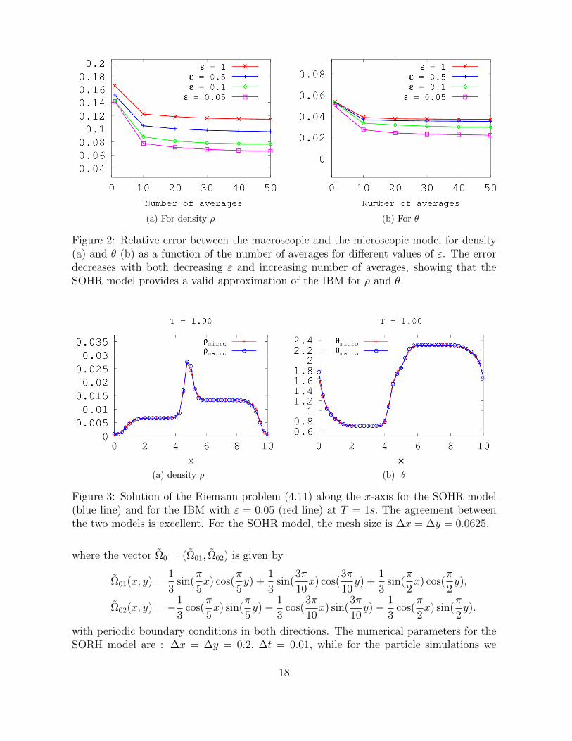
(a) For density ρ (b) For θ
Figure 2: Relative error between the macroscopic and the microscopic model for density(a) and θ (b) as a function of the number of averages for different values of ε. The errordecreases with both decreasing ε and increasing number of averages, showing that theSOHR model provides a valid approximation of the IBM for ρ and θ.
(a) density ρ (b) θ
Figure 3: Solution of the Riemann problem (4.11) along the x-axis for the SOHR model(blue line) and for the IBM with ε = 0.05 (red line) at T = 1s. The agreement betweenthe two models is excellent. For the SOHR model, the mesh size is ∆x = ∆y = 0.0625.
where the vector Ω0 = (Ω01, Ω02) is given by
Ω01(x, y) =1
3sin(
π
5x) cos(
π
5y) +
1
3sin(
3π
10x) cos(
3π
10y) +
1
3sin(
π
2x) cos(
π
2y),
Ω02(x, y) = −1
3cos(
π
5x) sin(
π
5y)− 1
3cos(
3π
10x) sin(
3π
10y)− 1
3cos(
π
2x) sin(
π
2y).
with periodic boundary conditions in both directions. The numerical parameters for theSORH model are : ∆x = ∆y = 0.2, ∆t = 0.01, while for the particle simulations we
18

choose : N = 105 particles, ε = 0.05, r = 0.04, R = 0.2. In figure 4 and 5, we report thedensity ρ and the flux direction Ω at time t = 0.6s. In both figures, the left picture is forthe IBM and the right one for the SOHR model. Again, we find a very good agreementbetween the two models in spite of the quite complex structure of the solution.
(a) density ρ for the IBM (b) density ρ for the SOHR model
Figure 4: Density ρ for Taylor-Green vortex problem 4.12 at time t = 0.6s. Left: IBM.Right: SOHR model.
(a) Ω for the IBM (b) Ω for the SOHR model
Figure 5: Mean direction Ω for Taylor-Green vortex problem 4.12 at time t = 0.6s. Left:IBM. Right: SOHR model.
4.3 Comparison between the SOH and the SOHR model
In this part, we show the difference between the SOH system (1.6), (1.7) and the SOHRone for different values of the repulsive force Φ0. We recall that the SOHR model reduces
19

to the SOH one in the case in which the repulsive force is set equal to zero. To this aim,we rescale the repulsive force Φ0 by
Φ0 = F0
∫x∈R2
φ(x)dx
and then we let F0 vary. The repulsive potential φ is still given by (4.9), so that Φ0 =F0π/6. The other numerical parameters are chosen as follows: d = 0.05, α = 0, k0 = 1/8,µ = 1, Lx = 10, Ly = 10, ∆x = ∆y = 0.15, ∆t = 0.001. The initial data are those of thevortex problem (4.10) except that we start with four vortices instead of only one. Periodicboundary conditions in both directions are used.
Figure (6) displays the solutions for the SOHR system for the density (left) and forthe flux direction (right) at T = 1.5s with F0 = 5. Figure (7) displays the solutions forF0 = 0.05. The results are almost undistinguishable to those of the SOH model (F0 = 0)and are not shown for this reason. These figures show that when the repulsive force islarge enough, the SOHR model can prevent the formation of high concentrations. Bycontrast, when this force is small, the SOHR model becomes closer to the SOH one andhigh concentrations become possible.
(a) density ρ for F0 = 5 (b) Ω for F0 = 5
Figure 6: Solution of the SOHR model for F0 = 5. Density ρ (fig 6a ), flux direction Ω(fig.6b ) at t = 1.5s.
4.4 Comparison between the SOHR and the DLMP model
In this final part, we want to compare the SOHR system to the hydrodynamic modelproposed by Degond, Liu, Motsch and Panferov in [12] (referred to as DLMP model).This model is derived, in a similar fashion as the SOHR model, starting from a system ofself-propelled particles which obey to alignment and repulsion. The main difference is thatin the DLMP model, the particle velocity is exactly equal to the self propulsion velocitybut the particles adjust their orientation to respond to repulsion as well as alignment.
20

(a) density ρ for F0 = 0.05 (b) Ω for F0 = 0.05
Figure 7: Solution of the SOHR model for F0 = 0.05. Density ρ (fig 6a ), flux direction Ω(fig.6b ) at t = 1.5s.
The resulting model is of SOH type and is therefore written (1.6), (1.7), but with anincreased coefficient in front of the pressure term PΩ⊥∇xρ, this coefficient being equalto v0 d(1 + d+c2
c1F0). The initial conditions and numerical parameters are the same as in
previous testIn figure 8, we report the density ρ (left) and the flux direction Ω (right) for F0 = 5
for the DLMP model. Comparing figures (6) with figure 8, we observe that the solutionsof the SOHR and of the DLMP model are different. The homogenization of the densityseems more efficient with the SOHR model than with the DLMP model. This can beattributed to the effect of the nonlinear diffusion terms that are included in the SOHRmodel but not in the DLMP model. Therefore, the way repulsion is included in the modelsmay significantly affect the qualitative behavior of the solution. In practical situations,when the exact nature of the interactions is unknown, some care must be taken to choosethe right repulsion mechanism.
5 Conclusion
In this paper, we have derived a hydrodynamic model for a system of self-propelled par-ticles which interact through both alignment and repulsion. In the underlying particlemodel, the actual particle velocity may be different from the self-propulsion velocity asa result of repulsion interactions with the neighbors. Particles update the orientation oftheir self-propulsion seeking to locally align with their neighbors as in Vicsek alignmentdynamics. The corresponding hydrodynamic model is similar to the Self-Organized Hy-drodynamic (SOH) system derived from the Vicsek particle model but it contains severaladditional terms arising from repulsion. These new terms consist principally of gradientsof linear or nonlinear functions of the density including a non-linear diffusion similar toporous medium diffusion. This new Self-Organized Hydrodynamic system with Repulsion
21

(a) density ρ (b) Ω
Figure 8: Solution of the DLMP model for F0 = 5. Density ρ (left) and flux direction Ω(right) at t = 1.5s.
(SOHR) has been numerically validated by comparisons with the particle model. It ap-pears more efficient to prevent high density concentrations than other approaches basedon simply enhancing the pressure force in the SOH model. In future work, this modelwill be used to explore self-organized motion in collective dynamics. To this effect, it willbe calibrated on data based on biological experiments, such as recordings of collectivesperm-cell motion.
References
[1] M. Aldana, V. Dossetti, C. Huepe, V. M. Kenkre, H. Larralde, Phase transitions insystems of self-propelled agents and related network models, Phys. Rev. Lett., 98(2007), 095702.
[2] I. Aoki, A simulation study on the schooling mechanism in fish, Bulletin of the JapanSociety of Scientific Fisheries, 48 (1982) 1081-1088.
[3] A. Baskaran, M. C. Marchetti, Nonequilibrium statistical mechanics of self-propelledhard rods, J. Stat. Mech. Theory Exp., (2010) P04019.
[4] E. Bertin, M. Droz and G. Gregoire, Hydrodynamic equations for self-propelled par-ticles: microscopic derivation and stability analysis, J. Phys. A: Math. Theor., 42(2009) 445001.
[5] F. Bolley, J. A. Canizo, J. A. Carrillo, Mean-field limit for the stochastic Vicsekmodel, Appl. Math. Lett., 25 (2011) 339-343.
[6] H. Chate, F. Ginelli, G. Gregoire, F. Raynaud, Collective motion of self-propelledparticles interacting without cohesion, Phys. Rev. E 77 (2008) 046113.
22

[7] Y-L. Chuang, M. R. D’Orsogna, D. Marthaler, A. L. Bertozzi and L. S. Chayes,State transitions and the continuum limit for a 2D interacting, self-propelled particlesystem, Physica D, 232 (2007) 33-47.
[8] I. D. Couzin, J. Krause, R. James, G. D. Ruxton and N. R. Franks, CollectiveMemory and Spatial Sorting in Animal Groups, J. theor. Biol., 218 (2002), 1-11.
[9] F. Cucker, S. Smale, Emergent behavior in flocks, IEEE Transactions on AutomaticControl, 52 (2007) 852-862.
[10] P. Degond, A. Frouvelle, J-G. Liu, Macroscopic limits and phase transition in asystem of self-propelled particles, J. Nonlinear Sci. 23 (2013), 427-456.
[11] P. Degond, A. Frouvelle, J-G. Liu, Phase transitions, hysteresis, and hyperbolicityfor self-organized alignment dynamics, preprint. arXiv:1304.2929.
[12] P. Degond, J-G. Liu, S. Motsch, V. Panferov, Hydrodynamic models of self-organizeddynamics: derivation and existence theory, Methods Appl. Anal., 20 (2013) 089-114.
[13] P. Degond, S. Motsch, Continuum limit of self-driven particles with orientation in-teraction, Math. Models Methods Appl. Sci., 18 Suppl. (2008) 1193-1215.
[14] P. Degond, P. F. Peyrard, G. Russo, Ph. Villedieu, Polynomial upwind schemes forhyperbolic systems, C. R. Acad. Sci. Paris, Ser I, 328 (1999) 479-483
[15] H.Fehske, R. Schneider and A. Weisse, Computational Many-Particle Physics,Springer Verlag, 2007.
[16] A. Frouvelle, A continuum model for alignment of self-propelled particles withanisotropy and density-dependent parameters, Math. Mod. Meth. Appl. Sci., 22(2012) 1250011 (40 p.).
[17] G. Gregoire, H. Chate, Onset of collective and cohesive motion, Phys. Rev. Lett., 92(2004) 025702.
[18] S. Henkes, Y. Fily, M. C. Marchetti, Active jamming: Self-propelled soft particles athigh density, Phys. Rev. E 84 (2011) 040301.
[19] J. P Hernandez-Ortiz, P. T Underhill, M. D. Graham, Dynamics of confined suspen-sions of swimming particles, J. Phys.: Condens. Matter 21 (2009) 204107.
[20] R. W Hockney and J. W Eastwood, Computer Simulation Using Particles. Instituteof Physics Publishing, 1988.
[21] D. L .Koch, G. Subramanian, Collective hydrodynamics of swimming microorgan-isms: Living fluids, Annu. Rev. Fluid Mech., 43 (2011) 637-59.
[22] A. Mogilner, L. Edelstein-Keshet, L. Bent and A. Spiros, Mutual interactions, po-tentials, and individual distance in a social aggregation, J. Math. Biol., 47 (2003)353-389.
23

[23] S. Motsch, L. Navoret, Numerical simulations of a non-conservative hyperbolic systemwith geometric constraints describing swarming behavior, Multiscale Model. Simul.,9 (2011) 1253-1275.
[24] S. Motsch, E. Tadmor, A new model for self-organized dynamics and its flockingbehavior, J. Stat. Phys., 144 (2011) 923-947.
[25] T. J. Pedley, N. A. Hill, J. O. Kessler, The growth of bioconvection patterns in auniform suspension of gyrotactic micro-organisms, J. Fluid. Mech., 195 (1988) 223-237.
[26] F. Peruani, A. Deutsch, M. Bar, Nonequilibrium clustering of self-propelled rods,Phys. Rev. E 74 (2006) 030904(R).
[27] V. I. Ratushnaya, D. Bedeaux, V. L. Kulinskii, A. V. Zvelindovsky, Collective be-havior of self propelling particles with kinematic constraints: the relations betweenthe discrete and the continuous description, Phys. A 381 (2007) 39-46.
[28] D. Saintillan, M.J. Shelley, Instabilities, pattern formation and mixing in active sus-pensions, Phys.Fluids 20 (2008) 123304.
[29] B.Szabo, G.J Szollosi, B. Gonci, Zs. Juranyi, D. Selmeczi, and T. Vicsek Phasetransition in the collective migration of tissue cells: Experiment and model, Phys.Rev. Lett, 74 (2006) 061908.
[30] J. Toner, Y. Tu and S. Ramaswamy, Hydrodynamics and phases of flocks, Annals ofPhysics, 318 (2005) 170-244
[31] T. Vicsek, A. Czirok, E. Ben-Jacob, I. Cohen, O. Shochet, Novel type of phasetransition in a system of self-driven particles, Phys. Rev. Lett., 75 (1995) 1226-1229.
[32] T. Vicsek, A. Zafeiris, Collective motion, Phys. Rep., 517 (2012) 71-140.
[33] F. G. Woodhouse, R. E. Goldstein, Spontaneous Circulation of Confined Active Sus-pensions, Phys. Rev. Lett. 109 (2012) 168105.
Appendix A Proof of formulas (2.14), (2.15)
By introducing the change of variable z = −x− y√εR
and using Taylor expansion, we get
1
(√εR)n
∫Sn−1×Rn
K( |x− y|√
εR
)f ε(y, ω, t)ω dω dy
=
∫Sn−1×Rn
K(|z|) f ε(x+√εRz, ω, t)ω dz dω
=
∫Sn−1×Rn
K(|z|)(f ε +
√εR∇xf
ε · z +εR2
2D2xf : (z ⊗ z) +O(
√ε
3))(x, ω, t)ω dz dω
=(J(x, t) + ε k0 ∆xJ(x, t) +O(ε2)
),
24

where k0 is given by (2.16) and D2xf is the Hessian matrix of f with respect to the variable
x. Here, we have used that the O(√ε) and O(ε3/2) terms vanish after integration in z by
oddness with respect to z.
By the same computation for the kernel φ, we have
1
(εr)n
∫Sn−1×Rn
φ(|x− y|εr
)f ε(y, ω, t)dydω
=
∫Sn−1×Rn
φ(|z|)f ε(x+ εrz, ω, t)dzdω
=
∫Sn−1×Rn
φ(|z|)(f ε + εr∇xf · z +O(ε2))(x, ω, t)dzdω
= Φ0
∫Sn−1
f ε(x, ω, t)dω +O(ε2),
with Φ0 =∫Rn φ(|z|)dz.
Appendix B Proof of Theorem 2.1
We prove that (2.34) leads to (2.25). Thanks to (2.30), Eq. (2.34) can be written:
PΩ⊥
∫ω∈S2
(T1(ρMΩ) + T2(ρMΩ) + T3(ρMΩ))h(ω · Ω)ωdω := T1 + T2 + T3 = 0, (B.1)
where T k, k = 1, 2, 3 are given by (2.33). Now, T1(ρMΩ) can be written:
T1(ρMΩ) = ∂t(ρMΩ) +∇x · (ωρMΩ)− Φ0∇x ·(∇x
(ρ2
2
)MΩ
). (B.2)
We recall that the first two terms of T1 at the right hand side of (B.2) and the corre-sponding terms in T1 have been computed in [13]. The computation for the third term ofT1 is easy and we get:
T1 = β1ρ∂tΩ + β2ρ(Ω · ∇x)Ω + β3PΩ⊥∇xρ+ β4(∇x
(ρ2
2
)· ∇x)Ω
where the coefficients are given by
β1 =1
d(n− 1)〈sin2 θ h〉MΩ
, β2 =1
d(n− 1)〈sin2 θ cos θ h〉MΩ
,
β3 =1
n− 1〈sin2 θ h〉MΩ
, β4 = − Φ0
d(n− 1)〈sin2 θ h〉MΩ
.
Now observe that for a constant vector A ∈ Rn, we have
∇ω(ω · A) = Pω⊥A, ∇ω · (Pω⊥A) = −(n− 1)ω · A. (B.3)
25

Thus, using (2.33), (B.3) and the chain rule, we get for T2(ρMΩ)
T2(ρMΩ) = αΦ0
((n− 1)ω · ∇x
(ρ2/2
)− d−1∇x
(ρ2/2
)· Ω
+d−1(ω · ∇x(ρ
2/2))(ω · Ω)
)MΩ
Finally, we obtain:
T2 = β5 PΩ⊥∇x
(ρ2
2
),
where
β5 = αΦ0
(〈sin2 θ h〉MΩ
+1
d(n− 1)〈sin2 θ cos θ h〉MΩ
).
The terms T3(ρMΩ) and T3 have been computed in [12]. In particular, it is easy to seethat we get them from the formulae for T2(ρMΩ) and T2 by changing −αΦ0∇x(ρ
2/2) intok0PΩ⊥∆x(ρΩ). Therefore, we get:
T3 = β6 PΩ⊥∆x(ρΩ),
where
β6 = −k0
(〈sin2 θ h〉MΩ
+1
d(n− 1)〈sin2 θ cos θ h〉MΩ
).
Inserting the expressions of T1, T2 and T3 into (B.1) we get (2.25).
Appendix C Proof of Proposition 3.1
We follow the lines of the proof of Proposition 3.1 of [23]. Assume that ρη → ρ0 andΩη → Ω0 as η tends to zero. Then, set
Rη := ρη(1− |Ωη|2)Ωη.
Multiplying equation (3.2) by η and then taking the limit η → 0 yields Rη → 0. It followsthat |Ω0|2 = 1. Since the vector Rη is parallel to Ωη, we have P(Ωη)⊥R
η = 0, which impliesthat
P(Ωη)⊥
(∂t(ρ
ηΩη) +∇x · (ρηV η ⊗ Ωη) +∇xp(ρη)− γ∆x(ρ
ηΩη))
= 0.
Therefore, letting η → 0, we obtain
∂t(ρ0Ω0) +∇x · (ρ0V 0 ⊗ Ω0) +∇xp(ρ
0)− γ∆x(ρ0Ω0) = βΩ0, (C.4)
where β is a real number, p(ρη)→ p(ρ0) = dρ0 +αΦ0(d+ c2)(ρ0)2/2, V 0 = c2Ω0−Φ0∇xρ0
and U0 = c1Ω0 − Φ0∇xρ0. By taking the scalar product of (C.4) with Ω0, we get
β = ∂tρ0 +∇x · (ρ0V 0) +∇xp(ρ
0) · Ω0 − γ∆x(ρ0Ω0) · Ω0.
Inserting this expression of β into (C.4) we find the equation for the evolution of theaverage direction (2.25) and thus the SOHR model (2.24)-(2.27).
26