October 2001

Macroeconomic Models of theInternational Monetary Fund andthe World Bank(Analysis of Theoretical Approaches andEvaluation of Their EffectiveImplementation in Bulgaria)

Vi c t o r Yo t z o v

BULGARIAN NATIONAL BANKdp

/1dp

/1dp

/1dp

/1dp

/1 4/2

000

4/20

004/

2000

4/20

004/

2000

DISC

USSIO

N PA

PERS

2

dp/

14/2

000

© Bulgarian National Bank, October 2001

ISBN 954 ≠ 9791 ≠ 50 ≠ 5

Printed in BNB Printing Center.

Views expressed in materials are those of the authors and do not necessarily

reflect BNB policy.

Send your comments and opinions to:Publications DivisionBulgarian National Bank1, Alexander Battenberg Square1000 Sofia, BulgariaTel.: 9145/1271, 1351, 1906Fax: (359 2) 980 2425e-mail: Dimova.L@bnbank.org

Website: www.bnb.bg

DISCUSSION PAPERSEditorial Board:Chairman: Garabed MinassianMembers: Roumen Avramov

Georgi PetrovSecretary: Lyudmila Dimova

3

Disc

ussion P

aper

s

Contents

1. The IMF Approach ........................................................................... 6

2. The World Bank Approach ............................................................ 12

3. The IMF and World Bank Merged Model ...................................18

Prices and Output ........................................................................... 19Monetary Sector ............................................................................. 19External Sector................................................................................ 20

4. Criticism of Applied Approaches .................................................. 22

5. Evaluation of the Results from ImplementedAdjustment Programs .................................................................24

References ............................................................................................34

4

dp/

14/2

000

Victor Yotzov is Head of Economic Research and Projections Directorate at BNB.The author thanks Prof. G. Minassian and colleagues from the Economic Research and

Projections Directorate for beneficial discussions.The author would welcome any comments. Yotzov.V@bnbank.org1 Polak, J. J. Monetary Analysis of Income Formation and Payments Problems. IMF

Staff Papers. Vol. 6, November 1957; Robichek, E. Walter. Financial Programming Exer-cises of the IMF in Latin America. Seminar in Rio de Janeiro, September 1967.

2 Currently the model is known as the RMSM-X (revised minimum standard model ≠extended). Here we will consider only its basic features so no difference will be made be-tween the two models, although they differ significantly in some aspects.

SUMMARY. IN THE PROCESS OF TRANSITION TO A MARKET ECONOMY BULGARIA ES-TABLISHED SUSTAINABLE RELATIONS WITH INTERNATIONAL FINANCIAL INSTITUTIONS,THE INTERNATIONAL MONETARY FUND AND THE WORLD BANK IN PARTICULAR. RE-LATIONS WITH THESE INSTITUTIONS ARE BASED ON IMPLEMENTATION OF SPECIFIC

PROGRAMS FOR ECONOMIC REFORMS. THIS PAPER PRESENTS AN ANALYSIS AND OVER-VIEW OF THE DIFFERENT APPROACHES TO ADJUSTMENT PROGRAM FORMULATION. IT

REVIEWS THE MACROECONOMIC MODELS OF THE IMF AND THE WORLD BANK,WHICH SERVE AS A BASIS FOR DEVELOPING SPECIFIC PROGRAMS. BASED ON THE STA-TISTICAL DATA FOR THE PERIOD SINCE THE START OF TRANSITION TO DATE AN AT-TEMPT IS MADE AT ASSESSING THE RESULTS AND EFFECTIVENESS OF ALL STANDBY

AGREEMENTS IMPLEMENTED BY BULGARIA OVER THE LAST TEN YEARS.

JEL classification: E41, F41, K42

The use of macroeconomic models in the process of designing,implementing and controlling programs supported by international fi-nancial institutions has a long history. Since their establishment in 1946the International Monetary Fund (IMF) and the World Bank (WB)have been called upon to provide financial support to their members.Credits are made after a comprehensive analysis of the reasons caus-ing the deficits (internal and/or external) and the necessary measuresto eliminate them. Based on the results from the analysis a specificprogram is developed aimed at restoring macroeconomic equilibrium.

The IMF approach to economic stabilization (generally referred toas financial programming) is based on the models designed in the1950s and 1960s by J. J. Polak and E. Walter Robichek.1 The theoreti-cal foundations of financial programming have remained generally un-changed for nearly 40 years. The RMSM model2 (revised minimum

5

Disc

ussion P

aper

s

standard model) is formulated by the World Bank in the late 1960s andearly 1970s and is based on contributions by Chenery, Strout, Weisskopfand Blomqvist3. Its theoretical background can be found in Harrod andDomarís two-gap growth model for an open economy.

Since the early 1970s, however, the conception and the structure ofadjustment programs have gradually evolved and expanded. In part,this reflects institutional and structural changes in the countries seekingsupport from international financial institutions. On the other hand,significant events occurred in the world economy4 that entailedchanges in the approach to program design. Since the early 1990s anew group of countries has emerged, collectively called ëtransitioneconomies.í It turned out that application of the standard model foranalysis and forecasting in transition economies produced weaker re-sults (according to the words of Polak himself).5

The IMF and WB models, though having different approaches toeconomic problems, have a common macroeconomic basis. Aneconomy is divided into four sectors, assuming that the private sectorhas all the factors of production. Revenue from sales of goods and ser-vices forms the income [Y] of the private sector, which is used for con-sumption [Cp], tax payment [T], and investment [∆K]. The remainingprivate sector income comprises accumulation of financial assets (sav-ings) which may take the form of money [∆M] and foreign assets [∆Fp]net of total banking system credits [∆Dp]. Therefore budgetary con-straints to the private sector are set by:

Y � T � Cp � ∆K ≡ ∆M + ∆F

p � ∆D

p(1).

The public sector uses resources collected from taxes for its ownconsumption [Cg], the remaining portion being financial assets in theform of foreign assets [∆Fg] net of banking system credits [∆Dg]:

T � Cg ≡ ∆F

g � ∆D

g(2).

3 Chenery, Hollis B., Alan M. Strout. Foreign Assstance and Economic Development.American Economic Review # 56, Sept. 1966; Weisskopf, Thomas E. The Impact of For-eign Capital Inflow on Domestic Savings in Underdeveloped Countries. Journal of Interna-tional Economics, Feb. 1972; Blomqvist, A. G. Empirical Evidence on the Two-Gap Hy-pothesis. Journal of Development Economics # 3, 1976.

4 Among the most important events are the end of the gold-dollar standard; the sharpprice rise in energy commodities and dramatic fluctuations in other goodsí prices; fast in-terest rate growth in international credit markets; reduced trade volumes and a slowdownin growth globally.

5 Polak J. J. The IMF Monetary Model at Forty. IMF Working Paper, WP/97/49.

6

dp/

14/2

000 The external sector receives income from imports6 of goods and ser-

vices [Z] and makes expenditure on exports of goods and services [X],the result being changes in net foreign assets of the private and publicsectors and in official foreign currency reserves [∆R]:

Z � X ≡ � (∆Fp

+ ∆F

g + ∆R) (3).

The banking system is represented only by the central bank which istreated as a financial intermediary acquiring assets in the form of offi-cial foreign currency reserves and loans to the private and public sec-tors, and liabilities in the form of money for the private sector:

∆M ≡ ∆R + ∆Dp +

∆D

g(4).

Combining budgetary constraints to the four sectors of the economy(1) ÷ (4), one obtains the generally known identity describing GDP fi-nal use:

Y � Cp � C

g � ∆K � X + Z ≡ 0 (5).

Based on these generally accepted macroeconomic relationshipsthe IMF and the World Bank have built two different approacheswhich, before being combined, need be summarized and distinguished.

1. The IMF ApproachSince IMF major goal is to support the balance of payments of

countries with chronic current account deficits, there is clearly the needto relate policy variables to foreign reserves dynamics. In this light, theIMF model sets an explicit relationship between variables controlledby the authorities and the balance of payments. This approach involvesexogenous setting of the nominal GDP:

Y = P y (6),

where

– is the price level, and y is real GDP7.In turn, a change in the nominal GDP [∆Y] is treated as resulting

from price and autonomous changes. Real GDP [y-1] and the pricelevel [P-1] in the previous period are known, the change in the pricelevel [∆P] is endogenous for the model, and growth [∆ y ] is set exog-

6 From external sector point of view imports represent income, while for the economythese are expenditures. The same approach applies to exports.

7 Although real GDP is set as an exogenous variable in the model, this does not meanthat in IMF programs it is treated likewise. Usually growth is derived from the simulta-neous assessment of structural changes and the external environment.

7

Disc

ussion P

aper

s

enously8:∆Y = ∆Py

-1 + P

-1∆ y (6').

Velocity of currency circulation [ν] is assumed as constant (or pre-dictable but outside the model framework) which gives ground to re-late money demand [Md] to income:

∆Md = ν∆Y (7).

It is also assumed that the money market is in equilibrium, whichmeans that money demand matches money supply [Ms], i.e.

∆Md = ∆Ms = ∆M (8).

Based on the last three equations and identity (4) the change in of-ficial foreign currency reserves can be presented as a function of exog-enous and policy variables:

∆R = ν∆Py-1

+ νP-1

∆ y � (∆ pD� + ∆ gD� ) (9),

where the sign ë^í above credits to private and public sectors definesthem as instrumental variables controlled by the monetary authorities.

Equation (9) illustrates the monetary approach to the balance ofpayments, presenting the change in official foreign currency reserves asthe difference between money supply and domestic credit. In formulat-ing a specific financial program the equation is resolved for a desiredvalue of the endogenous variable ∆R, and domestic credit growth is setas a ceiling. It is obvious that credit-ceiling setting depends to a largeextent on money supply. Therefore the sustainability of the money de-mand function is critical to the entire model.9

The inclusion of two endogenous variables [∆R and ∆P] in equation(9) means that by setting restrictions to domestic credit the solutionmay be found for any value of inflation, but this is not acceptable. In-cluding an additional behavioral equation relating GDP [Y] to imports[Z] solves the problem:

Z = αY = PyyPY D+D+--- 111 )( aa (10),

where α is the marginal propensity to import.

8 The combined impact of autonomous and price factors [∆P∆ y~ ] is considered negligi-bly small.

9 In order for changes in domestic credit to have a predictable effect on the balance ofpayments, money demand should be stable and be a function of a limited number of inde-pendent variables. However, this does not mean that the velocity of currency circulationshould be constant.

8

dp/

14/2

000

MM

BP

DRO

A

DR*B

∆R

∆P* ∆PO

∆P

Therefore reserves can also be derived from the combination ofequations (3), (6') and (10), and the relationship between reserves andchanges in the price level (inflation) is determined by another equa-tion:

∆R = PyyPYFX D-D+-D---- 111 )()( aa (11).

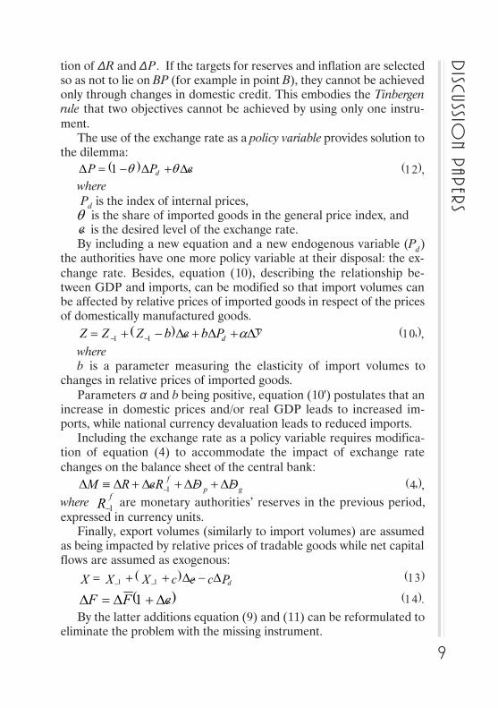
If the relationship between the balance of payments and monetaryand credit aggregates is presented graphically, assuming prices as anendogenous variable, it will look as follows:

Chart 1MONETARY APPROACH TO THE BALANCE OF PAYMENTS

(J. J. POLAK MODEL)

Equation (9) is described by ÃÃ line, and equation (11) is de-scribed by ¬– line. If we assume that equilibrium is achieved in point¿, domestic credit contraction will move ÃÃ upward left and the equi-librium point will move along the BP line in the same direction. Thismeans that forex reserves grow at lower values of inflation. The targetsfor reserves and inflation in this model cannot be taken independentlyof each other. Since changes in domestic credit can move the equilib-rium point only along ¬– line, D�D alone can influence the combina-

9

Disc

ussion P

aper

s

tion of ∆R and ∆ P . If the targets for reserves and inflation are selectedso as not to lie on ¬– (for example in point ¬), they cannot be achievedonly through changes in domestic credit. This embodies the Tinbergenrule that two objectives cannot be achieved by using only one instru-ment.

The use of the exchange rate as a policy variable provides solution tothe dilemma:

ePP d �)1( D+D-=D qq (12),

where Pd is the index of internal prices,q is the share of imported goods in the general price index, ande� is the desired level of the exchange rate.By including a new equation and a new endogenous variable (Pd)

the authorities have one more policy variable at their disposal: the ex-change rate. Besides, equation (10), describing the relationship be-tween GDP and imports, can be modified so that import volumes canbe affected by relative prices of imported goods in respect of the pricesof domestically manufactured goods.

yPbebZZZ d D+D+D-+=--

a�)( 11 (10'),

whereb is a parameter measuring the elasticity of import volumes to

changes in relative prices of imported goods.Parameters α and b being positive, equation (10') postulates that an

increase in domestic prices and/or real GDP leads to increased im-ports, while national currency devaluation leads to reduced imports.

Including the exchange rate as a policy variable requires modifica-tion of equation (4) to accommodate the impact of exchange ratechanges on the balance sheet of the central bank:

gpf DDReRM ��� 1 D+D+D+DºD-

(4'),

where fR 1- are monetary authoritiesí reserves in the previous period,

expressed in currency units.Finally, export volumes (similarly to import volumes) are assumed

as being impacted by relative prices of tradable goods while net capitalflows are assumed as exogenous:

dPcecXXX D-D++=--

�)( 11 (13)

)�1( eFF D+D=D (14).

By the latter additions equation (9) and (11) can be reformulated toeliminate the problem with the missing instrument.

10

dp/

14/2

000 )��(�)()1( 111 gp

fd DDyeRyPyR D+D-D+D-+D-=D

---nqnqn (9')

dPcbyecbFZXFZXR D+-D-D++D--+D--=D----

)(�)]([)( 1111 a (11').

This model is referred to as the expanded Polak model. It is ana-lyzed in the same way as the basic model, the only difference being thatthe abscissa in Chart 1 represents the change in domestic prices (∆Pd)alone. Essentially, controlling the change in the exchange rate )�( eDmakes it possible for BP line described by equation (11') to move sothat higher values of forex reserves can be achieved for a given level ofinflation. This allows for eliminating the requirement for setting re-straints to domestic credit and inflation only in combination so thatthey would always lie on BP line. Points outside BP (for example pointB) can be achieved through a change in the exchange rate so that BPpasses through point B, and control over domestic credit growth canmove MM to achieve the desired target.

The general structure of the model used by the IMF is given in thetable below.

Table 1STRUCTURE OF THE IMF MODEL

Targets Endogenous Exogenous Policy Parameters variables variables variables

∆ R ∆ Y ∆ y ∆D v ≠ velocity of currency in circulation

∆ Pd ∆M P f ∆ e a ≠ marginal propensity to import

∆ P X q ≠ share of imported goods in the price index

Z Z -1 b ≠ price elasticity of imports

∆ F ∆ Fp c ≠ price elasticity of exports

T ≠ Cg ∆F g

Constraints on domestic credit growth set by the policy variable(∆ D) usually take the form of ceilings. The IMF practice with standbyprograms has shown that instances of credit ceiling abuse are often dueto excessive growth in credit to the public sector. It is therefore com-mon practice to set constraints only to credit to the public sector,whereby credit to the private sector can be treated as an auxiliarypolicy variable )( *

pDD . This target is achieved by assuming public sec-

11

Disc

ussion P

aper

s

tor credit growth as a policy variable:*�pg DDD D-D=D (15).

Due to absent or underdeveloped stock markets in the countriesimplementing adjustment programs the relationship between GDP andcredit to private sector is generally positive and sufficiently strong. Thisgives grounds for assuming similar growth rates in nominal GDP andcredit to the private sector, making it possible to formulate a simplefunction of credit demand:

YYDD pp D=D-1

* )/( (16).

As regards budgetary restraints to the nonfinancial public sectorequation (16) fixes explicitly the admissible deficit since the modifica-tion (2') of equation (2):

ggg DFCT D-Dº- (2')means that the public sector will have to adjust to the fixed deficit byincreasing revenues and/or decreasing expenditures.

As the general structure of the model shows, it is focused on im-pacting demand rather than supply. Most IMF adjustment programsfocus on reducing absorption, considerable attention being paid to con-straining government expenditures. This approach is associated withexternalities ≠ restrictions on absorption affect income. Although theIMF is fully aware of the negative effects that a continuous contractionin demand may have, adjustment programs are still being applied by anumber of countries. Macroeconomic stabilization, being of decisiveimportance, is pointed out as a reason for applying adjustment pro-grams. It is assumed (although unproved) that favorable effects of in-ternal and external equilibrium are significantly greater than potentialincome losses.

The other approach in designing adjustment programs involves in-fluence on monetary aggregates. An understanding of the monetary na-ture of inflation underlies this approach. Provided aggregate spendingexceeds the production capacity of the economy (under the existingprice level) prices will increase to the equilibrium level. Usually this iseffected by decreasing the real value of financial assets. Conversely,the price level may decline (if prices are flexible tending downward),and (which is more likely) unemployment may rise or/and the degreeof production capacity utilization may fall, resulting in a reduced factorproductivity.

It is an elementary truth that two divergent targets cannot be

12

dp/

14/2

000 achieved employing one and the same instrument. Achievement of in-

ternal and external balance entails measures reducing internal spend-ing as well as measures aimed at restructuring general (internal andexternal) spending. Again, this is the real expression of the well-knownTinbergen rule10 that the number of employed instruments may not beless than the targets pursued. If absorption exceeds output, decreasedinternal demand releases inflationary pressure but this will hardly con-tribute to simultaneous internal and external balancing. The implemen-tation of the policy intended to both internal and external equilibriumwill result in a sizable income loss and increased social tension. In thiscase measures aimed to strengthen demand for local goods and ser-vices without increasing absorption should be taken. This can beachieved by implementing expenditure switching policy, particularly bya change in the exchange rate.

Combined implementation of restrictive and expenditure switchingpolicies poses the question of dichotomy between tradable and non-tradable goods which is considered an important analytical instrumentin studying depreciation or devaluation effects of the local currency11.Therefore, the philosophy of adjustment programs explains the reasonfor employing combined measures intended to reduce internal demandon the one hand, and measures encouraging exports and depressingimports, on the other hand. In turn, expenditure switching policy in-cludes various measures (a change in the exchange rate, price liberal-ization, lifting trade and nontrade constraints on foreign trade), in-tended to eliminate price discrimination of local goods and services.

In cases when GDP is smaller than targeted due to inefficient re-source allocation, the expenditure switching policy in respect of de-mand may also have a positive effect on the volume of output improv-ing output structure in terms of supply. Problems in designing and ap-plying growth-oriented programs are associated with the fact that ex-penditure switching policy entails a number of structural changes hav-ing uncertain effects and normally requiring a longer period of time.

10 Tinbergen, J. On the Theory of Economic Policy, North Holland, 1952.

11 The analysis aims at distinguishing tradable and nontradable goods rather than im-ported and exported goods as it is assumed that terms of trade are exogeniously set. SeeSwan, Trevor. Economic Control of Dependent Economy, Economic Record, vol. 36,1960.

13

Disc

ussion P

aper

s

2. The World Bank ApproachThe World Bank approach in applying expenditure switching policy

implies the use of effects from income reallocation. In contrast to IMFprograms focused primarily on achieving balance of payments equilib-rium, the World Bank is mostly involved in development projects ac-centing on medium-run economic growth. National accounts are tiedto the balance of payments. Concurrently, any emerging deficits andpossibilities for deficit financing should be carefully monitored. TheWorld Bank basic model focuses entirely on the real sector. Inflation isnot determined by the model itself (inflation is not an endogenous vari-able), and it is exogenously set. To simplify the presentation of themodel structure and comparison with the IMF model, it is assumedthat prices are constant (∆P = ∆ Pd = ∆P f = 0). In the context ofgeneral macroeconomic model, the World Bank approach requires in-clusion of four additional equations:

1. One of the major exogenous variables in the model is the ratio ofinvestment growth to GDP (ICOR ≠ incremental capital output ratio).

ICORt= 1

1

-

-

- tt

t

YY

I,

whereI is investment (gross capital formation), and Y is the gross domes-

tic product.This relationship is fundamental, as a significant deviation in its set-

ting predetermines the failure of the entire model. Simplicity is the ma-jor advantage of this approach, since no building of an individual in-vestment function is required in which capital stock occur as a vari-able12. However, simplification increases the risk of errors since impor-tant relationships are ignored:ï Increasing capacity utilization has a strong effect on ICOR forecast.

For example, other conditions being equal (i.e. if no increases incapital stock and investment occur) greater loading of existing ca-pacities will result in greater output volume and GDP respectively,prompting a decrease in ICOR values. Obviously, expectations fora change in intensity of utilizing existing production capacity shouldbe taken into account if ICOR is exogenously set.

12 Since evaluation of capital stock is difficult, it is recommendable to use informationon investments as it is much more reliable. If data on capital stock is comparatively reli-able, the relationship between capital stock and investments is expressed through theidentity K

t = K

t-1 + It ≠ A

t, where K is the capital stock, I investment and A amortization.

14

dp/

14/2

000 ï The structure of investment also has a strong effect on ICOR. Since

the dynamic relation between investment and GDP concerns onlytwo consecutive periods, it should not be expected that investment ininfrastructure projects, and that directed in output would equally re-late to growth. The same refers to the sectoral structure of invest-ment. Appropriate setting of ICOR necessarily entails distinguishinginvestment as its relationships to future growth significantly differ.It is assumed that the ratio of investment growth to output growth, i.

e. ICOR, is predetermined by past values or it may be forecast on thebasis of changes in the technological level of output. The concept ofICOR allows for expressing output volumes as a function of theamount of investment:

Ky D=D-1* r (17),

where∆  is investment (capital growth) and ρ is ICOR.This equation allows to determine growth based on available invest-

ment opportunities, or required investment to achieve the targetedgrowth rate.

2. Exports are set exogenously.3. The relationship between GDP and imports is assumed as

stable. The equation is similar to the IMF model equation (10) thoughexcluding price changes:

*yZ a= (10'')

4. The last equation supplementing the basic model includes thefunction of private sector savings. Under a set savings parameter thefunction of private sector consumption may be derived:

)�)(1( * TysC p --= ,where s is the ratio of private sector savings to disposable income.

Obviously, there are no significant differences between IMF andWorld Bank approaches regarding the external sector treatment. Majordifferences are as follows: the IMF uses the monetary approach ex-plaining balance of payments imbalances, while the World Bank fo-cuses on the real sector determining medium-term prospects for eco-nomic growth. The hypothesis of time constancy of investment growth/output growth ratio is based on a strongly restrictive assumption aboutthe nature of the aggregate production function. Commonly, treatmentof ICOR as a constant value is associated with the production function,with factors of production having constant weights, i. e. factor substitu-

15

Disc

ussion P

aper

s

tion is excluded. If factor substitution is assumed, ICOR will be a func-tion of the relationship between factor labor productivity and capitalproductivity, provided that general factor productivity is constant.

Problems associated with exogenously set ICOR resemble the prob-lems related to setting the velocity of currency circulation in the IMFmodel. Common in both cases is that constancy requirements are notabsolute, provided that the direction and intensity of changes in con-stancy requirements can be grounded and predicted to a large extent.The theory of economic growth factors is much richer than ICOR. Theeffects of technical progress and human capital are as important as in-vestment. Technically, the impact of these factors can be incorporatedinto ICOR. However, this requires precise evaluations and high degreeof economic intuition.

Based on the World Bank approach the basic identity (5) of incomecan be rewritten as

)()��()�( * XZCTCTyK gp -+-+--=D (19),

where internal investment is considered as a sum total of private andpublic sector savings plus the inflow (use) of external savings. Substi-tuting the private sector consumption function (18) and the import de-mand function (10'') in the latter equation, we obtain

)()��()�( ** XyCTTysK g -+-+-=D a (20).

Transforming the latter equation in order to outline growth, an al-ternative equation on investment based on the basic equation on in-come can be derived:

CTsysK g ---++=D ��)1()( *a X (5').

This equation shows the positive relationship between income andinvestment (parameters α and s are positive) through the aggregatedemand curve under exogenously set changes in the price level. In-come growth [y*] is accompanied both by increased domestic savings(under preset parameter s) and greater use of external savings, insofaras the marginal propensity to import [α] is positively linked to income.In other words, savings growth (both internal and external) results in aproportional increase in investment.

In respect of supply, income is determined by equation (17) on therelationship between production and investment which can be trans-formed as

1*

--=D yyK rr (17').

Consequently, we obtain one more equation expressing the positive

16

dp/

14/2

000 relationship between income (production) and investment which can

be graphically presented.Chart 2

PRODUCTION AND INVESTMENT ACCORDING TO THEWORLD BANK MODEL

AD

AS

B

A

DK

DK1

DKO

YO* Y1* Y

The slope of the line displaying aggregate supply (AS) is deter-mined by ICOR [ρ] from equation (17'), while the slope of aggregatedemand (AD) is determined by the sum total of (s + α) from equation(5'). As empirically obtained values of [ρ], based on a number of cross-country studies, vary between four and seven, and parameters s and αare positive but less than one, obviously the slope of the AS is largerthan the slope of AD. The government can move AD implementingparticular economic policy measures intended to change internal sav-ings. In the reviewed model (equation 5') the government has at its dis-posal only tax revenues and public sector expenditure. If point A is inequilibrium corresponding to a particular investment volume (∆Ko) un-der the targeted output volume ( *

0Y ), other conditions being equal, areduction in public sector expenditure will shift AD upward left, andthe new point of equilibrium (B) will correspond to a higher output vol-

17

Disc

ussion P

aper

s

ume ( *1Y ) and increased investment (∆K1). If the interest rate is also

included in the model, corresponding to a much greater degree to real-ity, the government will have one more instrument to influence aggre-gate demand. The eventual inclusion of the exchange rate as an instru-mental variable not only will move the aggregate demand curve up ordown but it will also change the curve slope, as any exchange ratemovement affects the marginal propensity to import (α). An increasein taxes prompts a growth in public sector savings and a fall in privatesector savings. The general effect on aggregate demand will tend todecline, since the private sector reacts to the lower disposable incomeby reducing consumption.

The policy variable of income growth (∆Y*) can be coordinatedwith the policy variable of foreign exchange reserves growth (∆ R*),provided that net capital flows are controlled or a trouble-free accessto capital markets is assumed. In this case net capital flows may betreated as an instrumental variable.

**� RyXF D--=D a (21).

The formulated model may be presented in accordance with thestandard classification of variables.

Table 2STRUCTURE OF THE WORLD BANK BASIC MODEL

Targets Endogenous Exogenous Policy Parameters variables variables variables

∆y* Z X Cg s ≠ private sectorsavings to disposable

income∆R* ∆ K T α ≠ marginal propensity

to importCp ∆ F ρ (ICOR)

As it has been already mentioned, the World Bank approach drawsits theoretical fundamentals from the two-gap growth model. Providedthere are any constraints on foreign financing, the latter equation (21)will actually present limited growth opportunities determined by equa-tions (5') and (17'). This group of models including constraints on netcapital flows, are known in theory as two-gap models. In this respectRMSM-X model is basically used to estimate the implications on eco-nomic growth under alternative levels of foreign financing.

However, from a technical point of view, inclusion of constraints on

18

dp/

14/2

000 net capital flows makes the model overdetermined,13 and the removal

of this defect requires inclusion of an additional policy variable: the ex-change rate. Similar to the IMF approach, import volumes depend notonly on income and marginal propensity to import but also on ex-change rate changes ( e� ) and elasticity of imports regarding changes inrelative prices.14 Exports are no longer a purely exogenous variable andare also dependent on exchange rate movements and elasticity of ex-ports to changes in relative prices.

ebyZ �*-=a (22)

and

ecX �= (23).

Therefore equation (21) describing net capital flows modifies into** �)( RecbyF D-++-=D a (24).

As a result, the model is entirely determined since exchange ratechanges can accommodate the income growth target and constraintson foreign financing. Prior to the inclusion of the exchange rate (underrestrictions on capital flows), the model contained only two endog-enous variables (Z and Cp) and three independent equations.

3. The IMF and World Bank Merged ModelBased on basic macroeconomic dependencies (equations 1 ÷ 5) and

divergent approaches applied by the IMF and the World Bank inspecifying particular macroeconomic models, Khan, Montiel andHague15 propose a model combining the advantages of both ap-proaches. The key relationship between the external sector and mon-etary and credit aggregates is sustained, while the disadvantage associ-ated with the lack of growth component and the impact of changes inrelative prices is removed.

13 Restriction on foreign financing (i.e. a deficit in respect of the external sector) resultsin overdetermination since internal savings can be obtained in two different ways. Undera set growth rate ICOR synonymously determines required investments. Provided the ac-cess to external savings is limited, internal savings appear as a residual value under al-ready determined investment volume. However, there is no guarantee that the obtainedinternal savings correspond to those obtained from equation (18).

14 As prices in the simplified model are assumed as constant, the change in the nominalexchange rate can also be interpreted as a change in the real exchange rate.

15 See Khan, M. S., P. Montiel and N. Haque (1990). Adjustment with Growth: Relatingthe Analytical Approaches of the IMF and the World Bank. Journal of Development Eco-nomics, #32, North-Holland, Khan, M. S., P. Montiel and N. Haque, eds. (1991) Macro-economic Models for Adjustment in Developing Countries. IMF, Washington, D.C.

19

Disc

ussion P

aper

s

The merged model includes three major segments.16

Prices and OutputGDP growth is set through its link with investments (ICOR) based

on equation (17):

P

Ky

D+

D=D

-

1

1* r

(17''),

where the nominal amount of investment is deflated by the increase inthe general price level and GDP growth is a policy variable.

Using identity (1) describing budget constraints on the private sec-tor, investment can be showed as:

ppd DFMTYYsK �)�( 1 D+D-D--D+ºD

-(1'),

where private sector savings are showed as a function of disposable in-come.

Budget constraints on the public sector are set using the basic iden-tity (2). The difference is that taxes [T] and government spending in thebasic model are considered as instrumental variables [Cg].

0)��( ºD+D-- ggg DFCT (2').

Similarly to the approach (6') used by the IMF, changes in thenominal amount of GDP include real and inflationary componentswith the real growth being a policy variable and not exogenously set asin the IMF approach:

1*

1 --D+DºD PyyPY (6'').

In the latter identity the change in the general price level is set simi-larly to equation (12), with the change in the internal price level consid-ered as a policy variable:

ePP d �)1( *D+D-=D qq (12').

Monetary SectorThe velocity of currency circulation [v] reflecting money demand is

assumed as an exogenously set parameter used to relate monetary ag-gregates to the nominal GDP:

∆Md = ν∆Y (7).

Money supply is obtained from the banking sector balance sheet(equation 4) under a targeted change in forex reserves and limited

16 The name of variables and numbering of equations are retained with a view to fol-lowing the economic logic in merging both models.

20

dp/

14/2

000 growth in credit to the private and public sectors.

gps

DDRM ��*D+D+DºD (4').

Money market equilibrium is set as an equation between money de-mand and money supply.

∆Ms = ∆Md = ∆M (8).

External SectorThe purpose of changing forex reserves is described by the balance

of payments as a balance between current and capital accounts:

)()(*gp FFZXR D+D--ºD (3').

Exports of goods and services are dependent on exchange ratechanges the internal price level and a parameter reflecting export elas-ticity to changes in relative prices, while changes in net capital flows inthe public and private sectors are exogenously set in units of foreigncurrency.

dPcecXXX D-D++=--

�)( 11 (13)

)�1( eFF pp D+D=D (14')

)�1( eFF gg D+D=D (14'').

Imports depend on GDP growth (income) as well as on the ex-change rate and relative prices:

**11 �)( yPbebZZZ d D+D+D-+=--

a (10'').

Table 3STRUCTURE OF THE IMF AND WORLD BANK MERGED

MODEL

Targets Endogenous Exogenous Policy Parameters variables variables variables

∆ y* ∆Y X-1

T (or Cg) ρ

∆ Pd* ∆P Z-1 pD�D θ∆ R* ∆ Ms

pFD gD�D v

∆ Md gFD e�D αX b

Z c

∆Fp

s

∆Fg

∆ K

T (or C g )

21

Disc

ussion P

aper

s

The merged model structure consists of 13 equations, including fiveidentities. Given the seven parameters set (estimated), these equationssynonymously determine the values of ten endogenous variables andthree policy variables depending on eight exogenous and instrumentalvariables. This is the so-called positive mode to solving the system ofequations used in building basic scenarios of the program which as-sumes stability in instrumental variables. The programming mode whichis used in formulating the programís final version starts with settingpolicy variables (which actually transform into exogenous). In this caseonly two instrumental variables can be set at random, the remaining in-strumental variables losing their independence, being determined bythe model.

As it has been already emphasized, IMF and World Bank ap-proaches have their own advantages and disadvantages. The attemptsto build a merged macroeconomic model are intended to remove dis-advantages while sustaining simplicity to a maximum degree. In thebasic IMF model also known as ëfinancial programming,í variablesconcerning the real sector are determined outside the model, while inthe World Bank model known as RMSM-X, inflation and changes inmonetary aggregates do not have direct effect on growth. The mergerof both approaches includes growth, inflation and forex reserves in thesystem of equations, formally transforming them into endogenous vari-ables, with the government having at its disposal (in the form of instru-mental variables) both fiscal and monetary variables. However, themerged model retains drawbacks and constraints typical of the modelístwo components. Some of these drawbacks, e.g. stability of the functionof money demand and ICOR, have been already discussed above. Prob-lems associated with the degree of conventionality and stability of otherparameters should not be underestimated. In principle, stability of pa-rameters in implementing any type of economic policy is a key factorfor reliability and forecasting strength of any macromodel (Lucas cri-tique). In addition to unavoidable problems associated with stability ofparameters, at least three more principle issues deserve attention.

The first refers to financial aspects of the model. Monetary sector(even in its extended version, i.e. including both the central and com-mercial banks) is presented only through variables concerning theamount of money, credit and forex reserves. No other forms of finan-cial assets are taken into account, and there is plenty of the financialsector of them in the economy. Therefore, the transmission mechanismof influence of the financial sector on the real sector is reduced to a

22

dp/

14/2

000

17 The lack of interest rates is even more surprising taking into account that one of themajor and traditional elements in IMF adjustment programs is the provision of positivereal interest rates used to influence the volume of internal savings.

level drifting it far away from the real functioning of the economy. Thelack of interest rates (an important element of the transmission mecha-nism) in the model is particularly sensitive among the set of instrumen-tal variables.17

The second issue is associated with the assumption that prices con-tinuously adjust thus maintaining money market equilibrium, that is atany moment money demand matches money supply. Unsoundness ofthis assumption is obvious as occurrence of lags in price adjustment isundoubtful.

The third issue stems from the fact that factors of production are notincluded in the function of growth. For instance, the lack of a wagelevel (change) is extremely sensible provided local currency devalua-tion is an important element of the implemented program. The objec-tive, that is the desired change in the exchange rate, proves impossibleto be realized using only fiscal and/or monetary instruments. This re-quires inclusion of additional equations establishing the relationshipbetween inflation and monetary incomes (wages) to make indicationsof the employment level, an essential element of the potential GDPamount.

4. Criticism of Applied ApproachesIt can be definitely concluded that IMF and World Bank models

and adjustment programs based on these models are often under thelash. The criticism sharpens in periods of international financial crises.A clear example of this was the Bretton-Woods financial system dis-ruption in the early 70s. The same happened as the debt crisis burst outin the early 80s and the socialist economic system disrupted at the endof the decade. As a result the ëclientsí of the IMF and World Bank dra-matically increased. After the financial crises in Mexico (1995) andAsia (1997 ≠ 1998), IMF and World Bank adjustment programs weremuch strongly criticized.

Most of the criticism has a populist character as it reflects the in-consistency between the public feeling and expectations, and the realresults from implemented adjustment programs. It is absolutely naturalfor the public to expect high growth rates, low inflation, increased em-ployment, social security, reduced taxes, etc. In the short run, realiza-

23

Disc

ussion P

aper

s

tion of public expectations prove impossible but the above goals are al-ways set in medium- and long-term programs. In a relatively short pe-riod adjustment programs can only overcome economic disequilibriumor at least reduce it. This can be achieved by:

ï providing external financing;ï pursuing conservative policy in respect of internal demand;ï implementing structural reform.These three elements constitute the core of any program, and the

models and their specification for a particular country are rather a mat-ter of technical skills.

Another critical trend concentrates on the theoretical ambiguity ofthe models. They cannot be synonymously associated with any moderntrend in the economic theory. Undoubtedly, the Keynessian spirit isdominating but there are also elements of neoclassicism, monetarismand even the theory of rational expectations. Eclecticism of modelscauses some problems, insofar as the models are of structural type.This requires indisputable causality relationship between variableswhich is not always available. However, the drawbacks of the eclecticapproach are offset by the goals set in programs. Macroeconomic mod-els of the IMF and World Bank are not intended to approve or reject aparticular economic theory. Therefore, no serious claims should be laidin respect of theoretical clearness.

Most often the models are criticized for insufficient specification ofany individual case which results in identical recommendations both bytype and ëdosageí. Unfortunately, it is impossible to check empiricallythe reliability of this hypothesis since no model specifications for othercountries are available. Regarding the complete identity of recommen-dations, this could hardly be the case. Studies carried out by the IMFand independent organizations reveal18 that ëdosageí depends both onthe type and degree of disequilibrium in the economy. For instance, theLatin American crisis in the early 80ís was characterized by huge fiscaldeficits resulting in chronically high inflation, slowdown, fast devalua-tion of the national currency and balance of payments deficits. Themeasures which had been taken in these countries were quite different

18 See for example, Dornbusch, R. Policies to Move from Stabilization to Growth, 1991,World Bank Research Report; Edwards, S. The IMF and the Developing Countries: ACritical Evaluation, 1989, Carnegie-Rochester Conference Series on Public Policy, #31,Elsevier, North-Holand; Dell, S. Stabilization: The Political Economy of Overkill, 1982,World Development, Oxford University Press; Mussa, M. and M. Savastano. The IMFApproach to Economic Stabilization. IMF Working Paper, WP/99/104, July 1999.

24

dp/

14/2

000 from those initiated against the financial crisis in some Asian countries.

In Asian countries the problems reflected mostly poor bank supervi-sion under conditions of a significant foreign investment inflow whichprompted a rapid increase in short-term liabilities and devaluationpressure.

In respect of the third important element in IMF and World Bankprograms (structural reforms) macromodels face serious difficulties inchoosing the most appropriate way of including the models in the sys-tem of equations. First of all the issue of the formal description of themodels should be solved. Some of required structural changes (liberal-ization or fixing of the exchange rate, providing positive interest rates,maximum admissible current account deficits and/or budget deficit,etc.) are comparatively easy to be carried out as this is a matter of ex-ogenous or endogenous setting. A number of structural changes (e.g.trade liberalization, improvement of bank supervision and accoun-tancy, establishment of market and nonmarket institutions, accelera-tion of privatization, etc.) are not subject to formal description. How-ever, these changes have a significant impact on the economy also inthe short run entailing their indirect inclusion in the models, whichmakes them highly vulnerable to criticism.

5. Evaluation of the Results from ImplementationAdjustment Programs

The history of economic reform in Bulgaria is closely tied to the his-tory of Bulgariaís relationships with the IMF and World Bank. Bul-garia has signed five standby agreements and one Extended Fund Fa-cility with the IMF. The general feeling is that experience and results ofimplemented IMF programs (at least until 1997) are not encouraging.This is clearly evidenced by the fact that only two (the first and thelast) of the five agreements were fully implemented. To this end, sev-eral important questions arise: the reason for the failure of most of theprograms; if the reason for the failure of these programs was due to aninadequately chosen approach (model) or the model was good but in-consistently implemented, with governments systemically failing to ful-fill undertaken commitments.

Special attention was paid to criticism that programs are stereo-typed based on restrictive monetary and fiscal policies, inconsistentwith the specificity of an individual country and disregarding growthproblems and social problems associated with them. Regarding gener-

25

Disc

ussion P

aper

s

ally unsatisfactory results entailing the introduction of a currency boardas an extreme measure to curb chronic inflation, it is quite easy to jointhe cohort of critics considering IMF models obsolete and inefficient.

In order to give adequate answers to the posed questions, it is nec-essary, though in brief, to review the major goals and results of allimplemented programs.

However, the following specifications should be made prior to thereview.

ï First, it is quite clear that there is no perfect model. Any model isbased on a number of assumptions associated with a particulareconomic theory. In this case the assumptions are based on theKeynnesian concepts of the government role and position ineconomic development. Perhaps, this is the bone of contentionas adherents of traditional Keynnesian theory have been pro-gressively losing ground in recent years.

ï Second, IMF and World Bank programs are related to theKeynnesian theory inasmuch as they seek to ensure governmentsupport in implementing required economic reforms. In this re-spect practical implementation of the programs proves impos-sible relying on monetary and fiscal policy instruments. As a rule(without any exceptions) countries requesting support from in-ternational financial institutions are underdeveloped, developingor transition economies with no experience in market economyand having no market-oriented institutions. No reliable statisti-cal information is available on most of the countries. Underthese conditions, design of macromodels taking into accountfluctuations in the business cycle as a result of technologicalshocks or including variables reporting changes in preferencesof economic agents and their rational expectations is absolutelyimpossible.

ï Third, IMF and World Bank models are based on generally ac-knowledged and indisputable economic interdependencies. Themodels are deliberately simplified and based on a limited num-ber of parameters, and rely to a great extent on instrumental andexogenous variables which should be treated as trends ratherthan as particular values.

ï Fourth, IMF and the World Bank are institutions with a specificpublic goal: supporting balance of payments of countries experi-encing serious temporary or chronicle deficits and promotingeconomic growth by implementing specific projects. It is quite

26

dp/

14/2

000 natural to extend loans under terms and conditions ensuring

loan repayment and avoiding recurrences. There is hardly agloomier prospective for a country than to become a permanentëclientí of international financial institutions. Despite seriouscriticism there is no other financial organization to propose abetter approach or more efficient programs. Recently there havebeen appeals to limit or even stop the IMF activity as the Fundísmeasures are always delayed and inadequately directed. It is of-ten heard that it would be more healthy for countries experienc-ing financial difficulties to overcome these difficulties by bor-rowing funds from financial markets.

The efficiency of implemented standby programs may be evaluatedby using various criteria and approaches:19

ï The before ≠ after approach used to evaluate countryís majormacroeconomic indicators prior to the launch of the programand those in the course of program implementation. However,the obvious simplicity of this approach is misleading as it as-sumes that all other parameters (i. e. macroeconomic variablesbeyond the scope of a particular program or set exogenously)stay unchanged. Since negative shocks can occur at any time(e.g. worsening terms of trade, increase in international financialmarket interest rates, unfavorable weather conditions), evalua-tions based on this approach may be (deliberately or not) inten-tional, in so far as all changes are associated with the imple-mented program. The problem with lags in program variablesíreaction is also essential.

ï The with ≠ without approach based on comparing economic re-sults of a particular country (or group of countries) implement-ing the program with results in another country (or group ofcountries) with similar problems which is not implementing sucha program. This approach overcomes the disadvantage of theprevious one where results from an implemented program arehard to be differentiated from autonomous and/or external fac-tors. However, the problem with unequal starting conditionsemerges, that is control country groups are not and may not beaccidentally chosen, since countries seeking financial support

19 This issue is thoroughly developed in: Haque, N., and M. Khan. Do IMF-SupportedPrograms Work? A Survey of the Cross-Country Empirical Evidence. IMF Working Pa-per, WP/98/169, Dec. 1998. Approaches for evaluating the efficiency of implementedprograms described below are based on the cited paper.

27

Disc

ussion P

aper

s

are generally in worse economic state. This also creates condi-tions for biased evaluations as far as it proves difficult to filterout program results from those due to different starting condi-tions. In such comparisons differences in the effect and directionof exogenous factors should also be taken into account.

ï The generalized evaluation approach includes comparison ofcountries or country groups implementing and not implementingprograms after the starting conditions and divergent effect ofexternal factors have been eliminated. This approach is compli-cated and its application limited as it is based on econometrictechniques intended to limit the model to equations (similar toequation [11']) representing the reduced form of the model. Theresults from solution of policy variable equations are compared,provided the government reaction in the countries not imple-menting the program is known on the basis of the reduced formof the model.

ï The comparison of simulations approach compares simulatedmacroeconomic indicators as a result of an implementedstandby program with the simulations resulting from the imple-mentation of another type of economic measures. This approachdirectly affects the quality of the applied model, since, unlike theprevious comparison approaches, simulations are used insteadof exact data considered as results from the implemented pro-gram. Difficulties in applying this approach are associated withthe need for a well approbated econometric model suitable forsimulation solutions, and the major problem relates to the well-known Lucas critique, postulating that parameters cannot staystable under significant changes in the economic policy pursued.

Evaluation of results from particular IMF and World Bank-sup-ported programs implemented in Bulgaria will be based on the first(before ≠ after approach) and partly on the fourth (the comparison ofsimulations) approach. The latter requires a review of the validity ofmajor assumptions and primarily of the correctness and stability ofused parameters. Based on statistical data for the 1990 ≠ 1998 periodthe following computations are made regarding:

ï the stability of money demand function (velocity of currency cir-culation);

ï the strength and stability of the relationship between import vol-umes and GDP;

28

dp/

14/2

000 ï inflation dependence on changes in the exchange rate and the

share of imported goods in the consumer basket;ï the validity of the hypothesis of a statistically important relation-

ship between real effective exchange rate indices and export vol-umes;

ï the accuracy of exogenous setting of GDP growth and net capi-tal inflow;

ï basic assumptions in compiling the state budget revenue side(buoyancy).

After reviewing the correctness of above computations, programsshould be compared with obtained results. Estimations should be madeof the extent to which discrepancies are due to incorrectly set exog-enous values, the extent to which they are due to violating preset re-quirements (instrumental variables) controlled by the government, aswell as of the extent to which these discrepancies reflect inherent andadmissible errors typical of any model. Only after that it can be arguedthat the model is wrong.

Evaluating the results from the implemented standby program, itshould be taken into account that programs do not coincide with calen-dar years which impedes the analysis of statistical data to a certain ex-tent.

The first standby agreement with the IMF was one-year, coveringthe period between 15 March 1991 and 15 March 1992. The agreementprovided for a purchase of SDR 279 million and SDR 60.6 million un-der the Compensatory and Contingency Financing Facility (CCFF) in-tended to compensate for the increased expenses on exports of energyinputs associated with the Persian crisis. As a result of nonfulfillment ofthe parameters under the agreement, the last tranche was not extended.

The second standby agreement was also one-year and provided fora purchase of SDR 155 million. The agreement became effective as of17 April 1992. The last tranche under this agreement was not disbursedas well.

The third standby agreement (one-year) was signed on 11 April1994, totaling SDR 69.7 million. In December 1994 the agreement wasrevised and extended by an additional SDR 69.7 million as a result ofthe agreement with the London Club creditors concluded in June 1994.The Systemic Transformation Facility (STF) of SDR 116.2 millionconcluded in April was also under the standby program implementedin this period. The last tranche of SDR 23.2 million was not disbursed.

The fourth agreement was signed on 19 July 1996 and provided for

29

Disc

ussion P

aper

s

a purchase of SDR 400 million for a period of 20 months (to 18 March1998). The agreement was terminated after the disbursement of thefirst tranche of SDR 80 million.

The fifth standby agreement was signed on 11 April 1997 and pro-vided for a purchase of SDR 371.9 million for a period of 14 months.The CCFF of SDR 107.6 million was also included in the fifth standbyagreement.

The last standby agreement with the IMF was signed on 25 Sep-tember 1998 for a three-year period. Financing under this agreement isexpected to total SDR 627.6 million. As the new agreement is inprogress, the results of its implementation have not been discussed.

Besides the agreements with the IMF between 1991 and 1998, theWorld Bank provided financing under special development projects.20

Funds disbursed by year and project are as follows:21

20 For a more detailed information about the World Bank projects in Bulgaria, see thewebsite of the World Bank representation in Bulgaria: http://www.worldbank.bg.

21 Besides these projects which have been finished, there are also programs underway,with funds under these programs still being utilized. Loans agreed under these programstotal USD 582 million, including USD 321 million until the end of 1998.

Project Effective Completed Amountas of on (million USD)

SAL I (Structural Adjustment Loan) IX.1991 IX.1994 250DDSR (Debt and Debt Servicing Loan) IX.1994 XII.1994 125ADP (Agricultural Development Loan) VII.1995 VI.1998 50PIEF (Private Investment and Export Finance) I.1994 VI.1998 55RL (Rehabilitation Loan) X.1996 VII.1997 30CIRL (Critical Imports Rehabilitation Loan) VIII.1997 VI.1998 40FESAL I (Financial and EnterpriseSector Adjustment Loan) I.1998 IV.1998 100TAL (Technical Assistance Loan) I.1992 VI.1999 17Telecommunications XII.1993 VI.1999 30

30

dp/

14/2

000 Table 4

EXOGENEOUS AND POLICY VARRIABLES IN STANDBYPROGRAMS

Projected Actual Projected Actual Projected Actual Projected Actual Projected Actual Projected Actual

First -11 -11.7 6.6 3.7 625 353.4 17 21.8 2.12 1.76 234 473.6Second -4 -7.3 3.9 3.9 1350 944.8 23.7 24.5 1.39 1.59 44 79.4Third -1÷ -2 1.8 4.2 3.9 1089 1006.4 59.6 66.0 1.62 1.59 74 121.9Fourth 0 -10.1 4.9 4.9 1327 488 150 487.4 1.83 1.33 105 310.8Fifth -7.4 -6.9 5 4.9 1947 2483 1700 1776.5 3.56 2.83 566 578.4

Agree-ment

GDP growth (%)

Exports(billion USD)

Forex reserves(million USD)

BGN/USDexchange rate

Velocity ofcurrency circulation

InflationDec. ≠ Dec. (%)

Table 6MAJOR ECONOMIC VARIABLES

Projected Actual Projected Actual Projected Actual Projected Actual

First -2 -1 -28.4 -56.2 24.1 24.7 8 3.8Second -1.4 -4.2 -1 18.9 33.9 50.1 4.3 4.2Third -4 -0.2 -18 -30.8 49.6 78.1 4.3 3.9Fourth 3.1 0.8 -13.5 -17.6 40.6 124.5 4.5 4.7Fifth 0.8 4.2 -23.5 -16.8 245.4 359.3 4.8 4.5

BOP current account(% of GDP) Real growth in wages (%) Broad money growth (%) Imports (billion USD)

Agreement

Agreement

Growth in bankingsystem NDA (%)

Real growth in creditto government

sector (%)

Real growth in creditto nongovernment

sector (%)Budget balance

(% of GDP)

Growth in BNBNFA

(million USD)

* Net domestic assets.** Net foreign assets.

Table 5PERFORMANCE CRITERIA

Projected Actual Projected Actual Projected Actual Projected Actual Projected Actual

First -103 -98 -65.0 -79.0 -48.4 -62.8 -3.5 -8.4 534 310.6Second - - 3.0 6.5 -9.7 -25.8 -4.2 -5.2 - -Third -27.4 -4.3 -24.0 -0.3 -24.1 -40.7 -6.3 -5.7 -600 -125.2Fourth 54.1 139.4 -36.0 -22.6 -45.0 -45.4 -4.7 -10.2 -235 -620Fifth 102.1 -24.8 -75.5 -73.2 -60.0 -32.2 -4.1 -2.9 620 1662

31

Disc

ussion P

aper

s

Statistical data displayed in Tables 4 ÷ 8 summarizes Bulgariaís ex-perience in implementing standby programs. All agreements imple-mented in Bulgaria are reviewed in chronological order with the excep-tion of the last three-year agreement concluded in September 1998which has not been completed yet. Since post-1989 transition to a mar-ket economy, 1994 and 1995 were the only two years when Bulgariadid not sign agreements with international financial institutions, and inboth cases the lack of financial support resulted in forex and financialcrises. Forex and financial crises burst out in the spring of 1994 and theautumn of 1996 and the government had to seek emergency support,signing imprecise agreements unable to settle the problems. Moreover,stopped financial support even worsened the existing problems. To thisend, it should be reminded that only the fifth agreement has been com-pleted, that is the total amount of funds provided under the agreementhas been disbursed to Bulgaria. The remaining agreements were un-timely terminated, as it was found during the regular quarterly reviewsthat Bulgaria failed to fulfill its commitments under the agreement, for-mulated as performance criteria. The fourth agreement was notlaunched practically, since it was terminated four months after its sign-ing, followed by a severe financial crisis. This evidenced again the cru-cial importance of external financing for Bulgariaís economy.

Table 4 displays exogenous and policy variables comparing the tar-gets set in the programs and actual results. It is easy to note that targetsand exogenously set values of major economic variables significantly

Table 7EFFECTIVENESS OF IMPLEMENTING PROGRAMS

AgreementInfaltion Forex GDP

Exports Velocity CGS*Exchange

Imports Ã3 CNS**reserves growth rate

First × × √ × × × × × √ ×Second × × × √ × × √ √ × ×Third × √ × × √ × × × × ×Fourth × × × √ × × × √ × √Fifth √ √ √ √ × √ √ √ × ×

** Credits to the government sector.** Credits to the nongovernment sector. × ≠ no effect from the program implementation. √ ≠ effect from program implementation.

Targets Exogeneous variables Policy variables Endogeneousvariables

32

dp/

14/2

000 diverge with few exceptions. This fact is of great importance as in this

case we are interested primarily in the principal ability of models togenerate forecasts during transition normally characterized by unstablemacroeconomic conditions rather than in the discrepancy between pro-jected and actual values. To this end, results summarized in Table 7 areindicative of the fact that preset goals were achieved only under thefifth standby agreement, that is performance criteria were strictly fol-lowed and exogenously set variables adequately selected.

Information contained in Table 8 is of particular interest as it dis-plays the effects of implemented programs both in the current and sub-sequent periods (after completion of the program). This evaluation ap-proach proves very important because standby programs are generallyintended to settle macroeconomic imbalances in the long run, not onlyfor the period of their implementation. Data suggests that an ad-equately designed program has also a favorable effect in the next pe-riod, while the programs which failed (clearly pronounced in the fourthstandby agreement) additionally worsen macroeconomic conditions.

The analysis of compliance with the performance criteria evidencesthe reasons behind the failure of all standby programs (except for thelast program). Even in cases of adequately selected policy and exog-enous variables, nonfulfillment of undertaken commitments con-demned these programs to failure. In most cases failures are associatedwith the programís (model) approach stating that it is unsuitable for thespecific Bulgarian conditions. However, data in Table 5 shows a differ-ent picture: due to various reasons (most often political, associatedwith pending elections and the ëneedí for saving the electorate the so-cial implications of reform) governments systemically escaped fromtheir responsibilities. Unfortunately, a number of important economicprerequisites (structural reform, legislation, institutional changes, etc.)which have no direct quantitative indicators but are crucially importantfor the implementation of the program cannot be included in the pub-lished tables. As a rule governments avoided painful decisions, thus re-ducing Bulgariaís chances for a faster completion of the delayed transi-tion.

33

Discussion PapersTable 8

MAJOR MACROECONOMIC VARIABLES BEFORE, DURING AND AFTER IMPLEMENTATION OF AD-JUSTMENT PROGRAMS

First, 1991 Second, 1992 Third, 1994 Fourth, 1996 Fifth, 1997Before Programs After Before Programs After Before Programs After Before Programs After Before Programs After

Growth (%) -11.8 -11.0 -7.3 -11.7 -4 -1.5 -1.5 -1 ∏ -2 2.1 2.1 0 -6.9 -10.1 -6.9 3.5Inflation (%) 64.5 234 79.4 473.6 44 63.8 63.8 74 32.9 32.9 105 578.4 310.8 566 1Forex reserves (million USD) 125 625 945 353.4 1350 655.3 655.3 1089 1241 1241 1327 2483 488 1947 3056Exports* (billion USD) 3.91 6.6 3.9 3.7 3.9 3.73 3.73 4.2 5.3 5.3 4.9 4.9 4.9 5 4.2Imports* (billion USD) 4.85 8.0 4.2 3.8 4.3 4.61 4.61 4.3 5.2 5.2 4.5 4.5 4.7 4.8 4.6Current account (% of GDP) -7.7 -2 -4.2 -1 -1.4 -8.7 -8.7 -4 2.1 2.1 3.1 4.2 0.8 0.8 -1

Budget balance (% of GDP) -8.5 -3.5 -5.2 -8.4 -4.2 -10.9 -10.9 -6.3 -6.4 -6.4 -4.7 -2.9 -10.2 -4.1 0.9Exchange rate (BGL/USD) 2.8 17 24.5 21.8 23.7 24.5 24.5 59.6 70.7 70.7 150 1776.5 487.4 1700 1675.1Real wage(real growth, %) 0.9 -28.4 18.9 -56.2 -1 1.1 1.1 -18 -5.5 -5.5 -13.5 -16.8 -17.6 -23.5 20.2Broad money/GDP 1.22 0.47 0.62 0.57 0.72 0.78 0.78 0.61 0.66 0.66 0.55 0.35 0.75 0.28 30.5

* Exports and imports for 1990 are recalculated at the exchange rate of 4.875 per 1 transferrable rouble.

34

dp/

14/2

000 References

Barth, R., and B. Chadha [1989] A Simulation Model for Financial Programming, IMF, WP/89/24.

Blomqvist, A. G. [1976] Empirical Evidence on the Two-Gap Hypothesis, Journal of Devel-opment Economics # 3.

Christoffersen, P., and P. Doyle [1998] From Inflation to Growth: Eight Years of Transition,IMF Working Paper, WP/98/100.

Edwards, S. [1989] The IMF and the Developing Countries: A Critical Evaluation, Carnegie-Rochester Conference Series on Public Policy, #31, Elsevier, North-Holland.

Fischer, S. [1997] Applied Economics in Action: IMF Programs, American Economic Asso-ciation (AEA) Papers and Proceedings, vol. 87, #2.

Fischer, S., R. Sahay and C. Végh [1998] From Transition to Market: Evidence and GrowthProspects, IMF Working Paper, WP/98/52.

Haque, N., and M. Khan [1998] Do IMF-Supported Programs Work? A Survey of the Cross-Country Empirical Evidence, IMF Working Paper, WP/98/169.

Havrylyshyn, O., I. Izvorski, and R. van Rooden [1998] Recovery and Growth in Transi-tion Economies 1990-97: A Stylized Regression Analysis, IMF Working Paper,WP/98/141.

IMF [1987] Theoretical Aspects of the Design of Fund-Supported Adjustment Programs,IMF, Occasional Paper 55.

IMF [1995] IMF Conditionality: Experience under Stand-By and Extended Arrangement. PartI: Key Issues and Findings, IMF. Occasional Paper 128, Washington D.C.

IMF [1995] IMF Conditionality: Experience under Stand-By and Extended Arrangement. PartII: Background Papers, IMF. Occasional Paper 129, Washington D.C.

Khan, M. S. and P. Montiel [1989] Growth-oriented Adjustment Programs: A ConceptualFramework, IMF Staff Papers, vol. 36, #2.

Khan, M. S., P. Montiel and N. Haque [1990] Adjustment with Growth: Relating the Analyti-cal Approaches of the IMF and the World Bank, Journal of Development Eco-nomics, #32, North-Holland.

Khan, M. S., P. Montiel and N. Haque (eds.) [1991] Macroeconomic Models for Adjustmentin Developing Countries, IMF, Washington D.C.

Leeper, E. M. and C. A. Sims [1994] Toward a Modern Macroeconomic Model Useable forPolicy Analysis, in O. Blanchard and S. Fischer (eds.) NBER MacroeconomicsAnnual, Cambridge, Mass.: MIT Press.

Lucas, R. E. [1976] Econometric Policy Evaluation: A Critique, in K. Bruner and A. Meltzer(eds.) The Phillips Curve and the Labor Market, Amsterdam: North-Holland.

Mussa, M. and M. Savastano [1999] The IMF Approach to Economic Stabilization. IMFWorking Paper, WP/99/104.

35

Disc

ussion P

aper

sPolak, J. J. [1957] Monetary Analysis of Income Formation and Payments Problems, IMF

Staff Papers, vol. 6.

Polak, J. J. and Victor Argy [1977] Credit Policy and the Balance of Payments, IMF StaffPapers, Vol.16.

Polak, J. J. [1997] The IMF Monetary Model at Forty, IMF Working Paper, WP/97/49.

Reinchart, C. [1991] A Model of Adjustment and Growth: An Empirical Analysis, in Macro-economic Models for Adjustment in Developing Countries, Khan M.,P. Montiel and N. Haque eds, IMF 1991.

Robichek, E. Walter [1967] Financial Programming Exercises of the IMF in Latin America,seminar in Rio de Janeiro.

Ìèíàñÿí, Ã., Ì. Íåíîâà è Â. Éîöîâ [1998] Ïàðè÷íèÿò ñúâåò â Áúëãàðèÿ, ÃîðåêñÏðåñ.

Ìèíàñÿí, Ã. [1999] Áúëãàðèÿ è Ìåæäóíàðîäíèÿò âàëóòåí ôîíä, Èêîíîìè÷åñêà ìèñúë,êí. 4.

Íåíîâñêè, Í. [1998] Òúðñåíåòî íà ïàðè â òðàíñôîðìèðàùèòå ñå èêîíîìèêè, Èçäàòåë-ñòâî íà ÁÀÍ, Ñîôèÿ.

Éîöîâ, Â. [1998] Âëèÿíèå íà âúíøíèÿ äúëã, ôèñêà è ïàðè÷íèòå àãðåãàòè âúðõóâàëóòíèÿ ñúâåò, â ñáîðíèêà „Áàíêîâèÿò ñåêòîð â óñëîâèÿòà íà âàëóòåíñúâåò“, Èíñòèòóò çà ïàçàðíà èêîíîìèêà, èçä. „Îòâîðåíî îáùåñòâî“.

36

dp/

14/2

000

DISCUSSION PDISCUSSION PDISCUSSION PDISCUSSION PDISCUSSION PAPERSAPERSAPERSAPERSAPERS

DP/1/1998 The First Year of the Currency Board in BulgariaVictor Yotzov, Nikolay Nenovsky, Kalin Hristov, Iva Petrova, Boris Petrov

DP/2/1998 Financial Repression and Credit Rationing under CurrencyBoard Arrangement for BulgariaNikolay Nenovsky, Kalin Hristov

DP/3/1999 Investment Incentives in Bulgaria: Assessment of the Net TaxEffect on the State BudgetDobrislav Dobrev, Boyko Tzenov, Peter Dobrev, John Ayerst

DP/4/1999 Two Approaches to Fixed Exchange Rate CrisesNikolay Nenovsky, Kalin Hristov, Boris Petrov

DP/5/1999 Monetary Sector Modeling in Bulgaria, 1913 – 1945Nikolay Nenovsky, Boris Petrov

DP/6/1999 The Role of a Currency Board in Financial Crises:The Case of BulgariaRoumen Avramov

DP/7/1999 The Bulgarian Financial Crisis of 1996 – 1997Zdravko Balyozov

DP/8/1999 The Economic Philosophy of Friedrich Hayek }(The Centenary of his Birth)Nikolay Nenovsky

DP/9/1999 The Currency Board in Bulgaria: Design, Peculiarities andManagement of Foreign Exchange CoverDobrislav Dobrev

DP/10/1999 Monetary Regimes and the Real Economy (Empirical Testsbefore and after the Introduction of the Currency Board in Bulgaria)Nikolay Nenovsky, Kalin Hristov

DP/11/1999 The Currency Board in Bulgaria: The First Two YearsJeffrey B. Miller

DP/12/1999 Fundamentals in Bulgarian Brady Bonds: Price DynamicsNina Budina, Tzvetan Manchev

DP/13/1999 Currency Circulation after Currency Board Introduction inBulgaria (Transactions Demand, Hoarding, Shadow Economy)Nikolay Nenovsky, Kalin Hristov