macroeconomic implications of the zero lower bound
TRANSCRIPT

Macroeconomic Implications of the Zero Lower Bound
by
Johannes Friedrich Wieland
A dissertation submitted in partial satisfaction of the
requirements for the degree of
Doctor of Philosophy
in
Economics
in the
Graduate Division
of the
University of California, Berkeley
Committee in charge:
Professor Yuriy Gorodnichenko, Chair
Professor Olivier Coibion
Professor Martin Lettau
Professor Maurice Obstfeld
Professor David Romer
Spring 2013


Abstract
Macroeconomic Implications of the Zero Lower Bound
by
Johannes Friedrich Wieland
Doctor of Philosophy in Economics
University of California, Berkeley
Yuriy Gorodnichenko, Chair
What policies are effective at combatting recessions when the zero lower bound(ZLB) binds? This dissertations contributes to this question in at least three ways.First, it examines several such policies in a standard macroeconomic framework.Second, it uses extensive robustness checks as well as macroeconomic and financialdata to validate or reject the key mechanisms that are at work in these models.Third, in the case of rejection, the standard framework is modified to match thedata and this improved framework is used to re-evaluate the policies in question.This produces new insights relative to existing literature that has largely remainedwithin the standard macroeconomic framework.
This dissertation first analyzes whether central banks should raise their infla-tion targets in light of the ZLB. It explicitly incorporates positive steady-state (or“trend”) inflation in standard macroeconomic models as well as the ZLB on nom-inal interest rates. For plausible calibrations with costly but infrequent episodesat the zero-lower bound, the optimal inflation rate is low, typically less than twopercent, even after considering a variety of extensions, including endogenous andstate-dependent price stickiness and downward nominal wage rigidities. The key in-tuition behind this result is that the unconditional cost of the zero lower bound issmall even though each individual ZLB event is quite costly. In short, raising theinflation target is too blunt an instrument to efficiently reduce the severe costs ofzero-bound episodes.
Second, this dissertation considers whether fiscal policy be effective in an openeconomy with flexible exchange rates. Standard open economy models suggest thatthe open economy fiscal multiplier is small when exchange rates are flexible. Thispremise is reassessed by explicitly incorporating the ZLB on nominal interest ratesin a small open economy New Keynesian model. It finds (1) when the ZLB bindsand uncovered interest rate parity (UIP) holds, then the open economy fiscal multi-plier is larger than 1 and bigger than the closed economy fiscal multiplier, (2) theseconclusions can be reversed given significant violations of UIP, and (3) for estimateddepartures from UIP, the open economy fiscal multiplier at the ZLB is above 1 butsmaller than the closed economy fiscal multiplier.
1

Third, this dissertation tests for a key propagation mechanism in standard macroe-conomic models — the inflation expectations channel. Accordingly, governmentspending multipliers are large and negative supply shocks are expansionary at theZLB because they lower expected real interest rates, which stimulates consumption.The second prediction is tested with oil supply shocks, an earthquake, and infla-tion risk premia, demonstrating that negative supply shocks are contractionary atthe ZLB despite also lowering expected real interest rates. These facts are rational-ized in a model with financial frictions. In this model demand-side policies, such asfiscal stimulus through government spending, are substantially less effective at theZLB than in standard sticky-price models, because raising inflation expectations byraising production costs is no longer a source of stimulus.
2

To my parents.
i

Contents
1 Introduction 11.1 Research Question . . . . . . . . . . . . . . . . . . . . . . . . . . . . 11.2 Methodology . . . . . . . . . . . . . . . . . . . . . . . . . . . . . . . 11.3 Contributions . . . . . . . . . . . . . . . . . . . . . . . . . . . . . . . 3
1.3.1 Should Central Banks Raise their Inflation Target? . . . . . . 31.3.2 How Large are Fiscal Multipliers? . . . . . . . . . . . . . . . . 41.3.3 Are Negative Supply Shocks Expansionary at the ZLB? . . . . 5
1.4 Overview of the dissertation . . . . . . . . . . . . . . . . . . . . . . . 7
2 The Optimal Inflation Rate in New Keynesian Models 82.1 Introduction . . . . . . . . . . . . . . . . . . . . . . . . . . . . . . . . 82.2 A New Keynesian Model with Positive Stead-State Inflation . . . . . 13
2.2.1 Model . . . . . . . . . . . . . . . . . . . . . . . . . . . . . . . 132.2.2 Steady-state and log-linearization . . . . . . . . . . . . . . . . 162.2.3 Shocks . . . . . . . . . . . . . . . . . . . . . . . . . . . . . . . 18
2.3 Welfare function . . . . . . . . . . . . . . . . . . . . . . . . . . . . . . 192.4 Calibration and Optimal Inflation . . . . . . . . . . . . . . . . . . . . 22
2.4.1 Parameters . . . . . . . . . . . . . . . . . . . . . . . . . . . . 222.4.2 Optimal Inflation . . . . . . . . . . . . . . . . . . . . . . . . . 252.4.3 Are the costs of business cycles and the ZLB too small in the
model? . . . . . . . . . . . . . . . . . . . . . . . . . . . . . . . 272.4.4 How does optimal inflation depend on the coefficient on the
variance of the output gap? . . . . . . . . . . . . . . . . . . . 282.5 Robustness of the Optimal Inflation Rate to Alternative Parameter
Values . . . . . . . . . . . . . . . . . . . . . . . . . . . . . . . . . . . 292.5.1 Pricing and Utility Parameters . . . . . . . . . . . . . . . . . 292.5.2 Discount Factor and Risk Premium Shocks . . . . . . . . . . . 312.5.3 Summary . . . . . . . . . . . . . . . . . . . . . . . . . . . . . 32
2.6 What could raise the Optimal Inflation Rate? . . . . . . . . . . . . . 332.6.1 Capital . . . . . . . . . . . . . . . . . . . . . . . . . . . . . . . 332.6.2 Model Uncertainty . . . . . . . . . . . . . . . . . . . . . . . . 34
ii

2.6.3 Downward Wage Rigidity . . . . . . . . . . . . . . . . . . . . 342.6.4 Taylor pricing . . . . . . . . . . . . . . . . . . . . . . . . . . . 352.6.5 Endogenous and State-Dependent Price Stickiness . . . . . . . 36
2.7 Normative Implications . . . . . . . . . . . . . . . . . . . . . . . . . . 382.7.1 Optimal Stabilization Policy . . . . . . . . . . . . . . . . . . . 382.7.2 Taylor Rule Parameters, Price-Level Targeting and the Opti-
mal Inflation Rate . . . . . . . . . . . . . . . . . . . . . . . . 392.8 Concluding Remarks . . . . . . . . . . . . . . . . . . . . . . . . . . . 40
3 Fiscal Multipliers at the ZLB: International Theory and Evidence 533.1 Introduction . . . . . . . . . . . . . . . . . . . . . . . . . . . . . . . . 533.2 An open economy model . . . . . . . . . . . . . . . . . . . . . . . . . 553.3 Fiscal Multipliers in the frictionless open economy . . . . . . . . . . . 583.4 Fiscal Multipliers in friction economy . . . . . . . . . . . . . . . . . . 623.5 Empirical Strategy & Results . . . . . . . . . . . . . . . . . . . . . . 65
3.5.1 Inflation Surprises . . . . . . . . . . . . . . . . . . . . . . . . 673.5.2 Exchange Rate Response to Inflation Surprises . . . . . . . . . 69
3.6 Quantitative analysis . . . . . . . . . . . . . . . . . . . . . . . . . . . 733.6.1 A model with capital . . . . . . . . . . . . . . . . . . . . . . . 75
3.7 Conclusion . . . . . . . . . . . . . . . . . . . . . . . . . . . . . . . . . 77
4 Are Negative Supply Shocks Expansionary at the ZLB? 794.1 Introduction . . . . . . . . . . . . . . . . . . . . . . . . . . . . . . . . 794.2 Predictions from Standard Sticky-Price Models . . . . . . . . . . . . 834.3 Negative Supply Shocks at the ZLB . . . . . . . . . . . . . . . . . . . 87
4.3.1 Oil Supply Shocks . . . . . . . . . . . . . . . . . . . . . . . . 874.3.2 The Great East Japan Earthquake . . . . . . . . . . . . . . . 91
4.4 Inflation Risk Premia at the ZLB . . . . . . . . . . . . . . . . . . . . 924.4.1 CCAPM Theory . . . . . . . . . . . . . . . . . . . . . . . . . 934.4.2 Estimated Inflation Risk Premia . . . . . . . . . . . . . . . . . 94
4.5 A Model with Financial Frictions . . . . . . . . . . . . . . . . . . . . 964.5.1 Households . . . . . . . . . . . . . . . . . . . . . . . . . . . . 974.5.2 Firms . . . . . . . . . . . . . . . . . . . . . . . . . . . . . . . 984.5.3 Banking Sector . . . . . . . . . . . . . . . . . . . . . . . . . . 994.5.4 Calibration . . . . . . . . . . . . . . . . . . . . . . . . . . . . 1014.5.5 Computation . . . . . . . . . . . . . . . . . . . . . . . . . . . 1024.5.6 Results . . . . . . . . . . . . . . . . . . . . . . . . . . . . . . . 103
4.6 Policy Implications . . . . . . . . . . . . . . . . . . . . . . . . . . . . 1054.7 Conclusion . . . . . . . . . . . . . . . . . . . . . . . . . . . . . . . . . 108
iii

A Appendix to Chapter 4 130A.1 Formal Solution . . . . . . . . . . . . . . . . . . . . . . . . . . . . . . 130
A.1.1 Case 1: No ZLB . . . . . . . . . . . . . . . . . . . . . . . . . . 131A.1.2 Case 2: The ZLB binds . . . . . . . . . . . . . . . . . . . . . . 131
A.2 Supply Shocks in the Smets-Wouters Model . . . . . . . . . . . . . . 133A.3 Inflation Expectations & Kalman Filter . . . . . . . . . . . . . . . . . 133
A.3.1 Data sources . . . . . . . . . . . . . . . . . . . . . . . . . . . . 135A.3.2 Kalman Filter . . . . . . . . . . . . . . . . . . . . . . . . . . . 137
A.4 Oil Shocks: Standard Error Correction . . . . . . . . . . . . . . . . . 140A.5 Oil Shocks: Robustness . . . . . . . . . . . . . . . . . . . . . . . . . . 141
A.5.1 4Q-Expectations Measured from Current Quarter . . . . . . . 141A.5.2 Inflation Expectations Measured from Inflation Swap Rates . . 141A.5.3 Eurozone . . . . . . . . . . . . . . . . . . . . . . . . . . . . . 143A.5.4 Additional Controls . . . . . . . . . . . . . . . . . . . . . . . . 143A.5.5 Lagged Dependent Variables . . . . . . . . . . . . . . . . . . . 143A.5.6 Outliers . . . . . . . . . . . . . . . . . . . . . . . . . . . . . . 147A.5.7 HP-filtered data . . . . . . . . . . . . . . . . . . . . . . . . . . 147A.5.8 NSA consumption . . . . . . . . . . . . . . . . . . . . . . . . . 147A.5.9 Excluding post-2006 data . . . . . . . . . . . . . . . . . . . . 150A.5.10 Lag Lengths . . . . . . . . . . . . . . . . . . . . . . . . . . . . 150
A.6 Oil Shocks: Event Study . . . . . . . . . . . . . . . . . . . . . . . . . 155A.7 Inflation Risk Premia . . . . . . . . . . . . . . . . . . . . . . . . . . . 158
A.7.1 s-year Inflation Risk Premia . . . . . . . . . . . . . . . . . . . 158A.7.2 Epstein-Zin Inflation Risk Premia . . . . . . . . . . . . . . . . 161
A.8 Swap Rate - Inflation Expectation Matching . . . . . . . . . . . . . . 163A.9 Supply Shocks and Credit Frictions . . . . . . . . . . . . . . . . . . . 163
A.9.1 Oil Supply Shocks . . . . . . . . . . . . . . . . . . . . . . . . 163A.9.2 Technology Shocks . . . . . . . . . . . . . . . . . . . . . . . . 166
A.10 Oil Shocks in Incomplete Markets . . . . . . . . . . . . . . . . . . . . 168A.10.1 Set-up . . . . . . . . . . . . . . . . . . . . . . . . . . . . . . . 168A.10.2 Equilibrium . . . . . . . . . . . . . . . . . . . . . . . . . . . . 170A.10.3 Computation . . . . . . . . . . . . . . . . . . . . . . . . . . . 171A.10.4 Foreign Economy . . . . . . . . . . . . . . . . . . . . . . . . . 172A.10.5 Home Economy . . . . . . . . . . . . . . . . . . . . . . . . . . 173
A.11 Model Solutions . . . . . . . . . . . . . . . . . . . . . . . . . . . . . . 175A.11.1 Accuracy of State Space Reduction . . . . . . . . . . . . . . . 175A.11.2 Accuracy of Non-linear Solution . . . . . . . . . . . . . . . . . 176
iv

B Appendix to Chapter 3 181B.1 Complete Model . . . . . . . . . . . . . . . . . . . . . . . . . . . . . . 181
B.1.1 Households . . . . . . . . . . . . . . . . . . . . . . . . . . . . 181B.1.2 Final Goods Firms . . . . . . . . . . . . . . . . . . . . . . . . 182B.1.3 Intermediate Goods Firms . . . . . . . . . . . . . . . . . . . . 184B.1.4 Government . . . . . . . . . . . . . . . . . . . . . . . . . . . . 184B.1.5 Prices and Market Clearing . . . . . . . . . . . . . . . . . . . 185
B.2 Backus-Smith with Wedge: An Example . . . . . . . . . . . . . . . . 186B.3 Solution Method for Baseline Model . . . . . . . . . . . . . . . . . . . 187B.4 Large Open Economy . . . . . . . . . . . . . . . . . . . . . . . . . . . 188B.5 The Nature of Inflation Surprises . . . . . . . . . . . . . . . . . . . . 189B.6 Supplemental Tables for Empirical Section . . . . . . . . . . . . . . . 194B.7 Taylor Rule Estimation . . . . . . . . . . . . . . . . . . . . . . . . . . 194
v

List of Tables
2.1 Baseline parameter values . . . . . . . . . . . . . . . . . . . . . . . . 422.2 Model fit at the baseline parameterization . . . . . . . . . . . . . . . 43
3.1 Correlation of Inflation Surprise with US Inflation. . . . . . . . . . . 683.2 Persistence of Inflation Surprise in Revised Inflation (Monthly Fre-
quency). . . . . . . . . . . . . . . . . . . . . . . . . . . . . . . . . . . 693.3 Exchange Rate Response to Inflation Surprises . . . . . . . . . . . . . 72
4.1 ZLB Dates . . . . . . . . . . . . . . . . . . . . . . . . . . . . . . . . . 1114.2 Parameterization of the Friction Model . . . . . . . . . . . . . . . . . 118
A.1 Inflation Expectations Data Sources . . . . . . . . . . . . . . . . . . . 136A.2 Impact of Oil Shocks on Macroeconomic Variables for Various Lags of
Oil Shocks in Equations (4.7) and (4.8). . . . . . . . . . . . . . . . . 154A.3 Swap Rate - Inflation Expectations Matching . . . . . . . . . . . . . 163A.4 Response of Japanese Bond Rate and Loan Spread to Oil Supply Shock167
B.1 Price Indices used for Inflation Surprises . . . . . . . . . . . . . . . . 194B.2 Inflation Surprises (YoY) . . . . . . . . . . . . . . . . . . . . . . . . 195B.3 Core Inflation Surprises (YoY) . . . . . . . . . . . . . . . . . . . . . 195B.4 Percentage Change in Exchange Rate after Inflation Announcements 196B.5 Episodes Classified as Liquidity Traps . . . . . . . . . . . . . . . . . . 197B.6 Taylor rule estimates . . . . . . . . . . . . . . . . . . . . . . . . . . . 198
vi

List of Figures
2.1 Frequency of being in the zero lower bound and steady-state nominalinterest rate. . . . . . . . . . . . . . . . . . . . . . . . . . . . . . . . . 44
2.2 Utility at different levels of steady-state inflation . . . . . . . . . . . . 452.3 The sources of utility costs of inflation . . . . . . . . . . . . . . . . . 462.4 The costs of business cycles . . . . . . . . . . . . . . . . . . . . . . . 472.5 Sensitivity: pricing parameters, habit, and labor supply elasticity . . 482.6 Sensitivity: risk premium shocks and the discount factor . . . . . . . 492.7 Robustness . . . . . . . . . . . . . . . . . . . . . . . . . . . . . . . . 502.8 Endogenous and state-dependent price stickiness . . . . . . . . . . . . 512.9 Positive implications: optimal policy . . . . . . . . . . . . . . . . . . 52
3.1 Fiscal multipliers for the baseline and friction model in normal timesand at the ZLB. . . . . . . . . . . . . . . . . . . . . . . . . . . . . . . 74
3.2 Fiscal multipliers for the capital model. . . . . . . . . . . . . . . . . . 76
4.1 Impact of negative supply shock in Euler equation framework of Sec-tion 4.2 . . . . . . . . . . . . . . . . . . . . . . . . . . . . . . . . . . 109
4.2 Impulse Response Functions to negative oil supply shocks . . . . . . . 1104.3 Change in nominal bond yield on impact of an oil supply shock . . . 1114.4 Impulse Response Functions to oil supply shocks 1985-present when
ZLB binds (“Baseline”) and when policy rates are unconstrained (“Nor-mal Times”). . . . . . . . . . . . . . . . . . . . . . . . . . . . . . . . 112
4.5 Consensus Economics forecasts from before Japanese Great Earth-quake (February 2011) and after (April 2011) . . . . . . . . . . . . . 112
4.6 Inflation Risk Premia for the U.K., Eurozone, and the U.S. . . . . . . 1134.7 Impact of negative supply shock at ZLB when these shocks have en-
dogenous negative demand effects, as in the friction model of Section 4.51144.8 Model solutions for log aggregate consumption lnC(a(t)) and inflation
π(a(t)) as a function of the technology shifter a(t). . . . . . . . . . . 1154.9 Model solutions for asset prices, marginal value of net worth, the bor-
rowing spread and the inflation risk premium as a function of thetechnology shifter a(t) . . . . . . . . . . . . . . . . . . . . . . . . . . 116
vii

4.10 Percentage change in output on impact for each basis point change inthe 10-year bond rate (left panel) and impact fiscal multiplier (rightpanel) . . . . . . . . . . . . . . . . . . . . . . . . . . . . . . . . . . . 117
A.1 Impulse response function for output to a one-standard-deviation tech-nology shock in the Smets and Wouters (2007) model. . . . . . . . . . 134
A.2 Impulse Response Functions to Oil Shocks for inflation expectationsderived from smoothed estimates (“Baseline”) and for inflation expec-tations derived from the one-sided filter. . . . . . . . . . . . . . . . . 139
A.3 Impulse Response Functions to Oil Shocks for 4-quarter ahead infla-tion expectations measured from the current quarter. . . . . . . . . . 142
A.4 Contemporaneous change in the inflation swap rate three months afteran oil supply shock has hit the economy (γ3 in Equation (4.7)). . . . 144
A.5 Impulse Response Functions to Oil Shocks excluding the Eurozonefrom the sample. . . . . . . . . . . . . . . . . . . . . . . . . . . . . . 145
A.6 Impulse Response Functions to Oil Shocks controlling for inflation andcorporate bond spreads. . . . . . . . . . . . . . . . . . . . . . . . . . 146
A.7 Impulse Response Functions to Oil Shocks excluding lagged dependentvariables in Equations (4.7) and (4.8). . . . . . . . . . . . . . . . . . 148
A.8 Impulse Response Functions to Oil Shocks excluding outliers based onjackknifed residual with 1% critical value. . . . . . . . . . . . . . . . 149
A.9 Impulse Response Functions to Oil Shocks for HP-filtered variables. . 150A.10 Impulse Response Functions to oil supply shocks over 1984-now when
ZLB binds (“Baseline”) and when policy rates are unconstrained (“Nor-mal Times”) for HP-filtered variables. . . . . . . . . . . . . . . . . . . 151
A.11 Impulse Response Functions of NSA consumption for Japan. . . . . . 152A.12 Impulse Response Functions to Oil Shocks excluding post-2006 data. 153A.13 Consensus Economics forecasts from before the Libyan uprising (Febru-
ary 2011) and after (March 2011). . . . . . . . . . . . . . . . . . . . 156A.14 Consensus Economics forecasts from before foreign intervention in the
Libyan civil war (March 2011) and after (April 2011). . . . . . . . . . 157A.15 Weight on inflation risk premia for various maturities and values of ρu, the
mean-reversion of supply shocks, when the state of the economy (ZLB or
non-ZLB) persists permanently. . . . . . . . . . . . . . . . . . . . . . . 159A.16 Inflation risk premia for various maturities and values of ρu (the mean-
reversion of supply shocks) when there is stochastic exit from the ZLB.. . . . . . . . . . . . . . . . . . . . . . . . . . . . . . . . . . . . . . . 161
A.17 Impact of oil shocks on credit standards in Japan. . . . . . . . . . . 165A.18 TFP Shocks and Credit Spreads . . . . . . . . . . . . . . . . . . . . . 169
viii

A.19 IRFs of Standard NK model, Friction Model with Three State Vari-ables, and Friction Model with One State Variable to a 1% TFP shock.. . . . . . . . . . . . . . . . . . . . . . . . . . . . . . . . . . . . . . . 177
A.20 IRFs of Friction Model with Three State Variables and Friction Modelwith One State Variable to a 1% TFP shock assuming that ZLB doesnot bind. . . . . . . . . . . . . . . . . . . . . . . . . . . . . . . . . . 178
A.21 IRFs of Friction Model with Three State Variables and Friction Modelwith One State Variable to a 1% TFP shock when the ZLB binds. . 179
A.22 Residuals of dynamic equations in non-linear solution. . . . . . . . . . 180
B.1 Domestic fiscal multipliers . . . . . . . . . . . . . . . . . . . . . . . . 190B.2 Predictive Power of Inflation Suprises . . . . . . . . . . . . . . . . . . 192B.3 Impulse Response Functions for inflation, unemployment, and central
bank nominal interest rates. . . . . . . . . . . . . . . . . . . . . . . . 193B.4 Predicted Policy Rates from Taylor Rule Estimates . . . . . . . . . . 199
ix

Acknowledgments
It is difficult to convey in words my gratitude towards my advisor, Yuriy Gorod-nichenko. Yuriy has spent countless hours giving me advice, encouragement, andsupport throughout my time at Berkeley, and this dissertation would not have beenpossible without him. I am also very much indebted to my committee membersOlivier Coibion, Pierre-Olivier Gourinchas, Martin Lettau, Maurice Obstfeld, andDavid Romer. They are truly exceptional teachers and mentors, and I have beenvery fortunate to benefit from their advice.
I owe much to my fellow graduate students at Berkeley. Especially DominickBartelme, Gabe Chodorow-Reich, Josh Hausman, Lorenz Kueng, John Mondragon,and Mu-Jeung Yang have not only been great friends but a constant source of en-couragement and advice. I have learned much from them, particularly during ourdaily lunch and office discussions, and I will very much miss them.
I would also like to thank Patrick Allen for his invaluable help in maneuveringthe Berkeley bureaucracy over the last five years.
Above all, I am grateful to my family. My parents, Gerlinde and Ulrich, havebeen patient and supportive throughout this endeavor. I only wish that I could haveseen them and Philipp more often. And I am deeply grateful to Lisa for always beingthere for me, during good and bad times.
x

Chapter 1
Introduction
1.1 Research Question
The zero lower bound (ZLB) on nominal interest rates has been a key constraint insome of the largest downturns in economic history — the Great Depression, the “LostDecade” in Japan, and the current economic crisis. With standard monetary policyrunning out of ammunition, different policies are required to mitigate the economicslump. But there is wide disagreement among policy makers and academics aboutwhat those policies should be and how effective they are. For instance, some policymakers and economists argue in favor of fiscal stimulus (e.g., Christiano, Eichenbaum,and Rebelo (2011), Eggertsson and Krugman (2011), Woodford (2012)), forwardguidance (e.g., Eggertsson and Woodford (2003, 2004), Bernanke (2012)), restrictingpotential output (Eggertsson (2011, 2012)), and allowing for permanently higherinflation targets (Blanchard, Dell’Ariccia, and Mauro (2010); Ball (2013)). However,others disagree that such discretionary policies are effective (e.g., Cochrane (2009))or desirable (Taylor (2012)). In this dissertation I attempt to contribute to thisdebate.
1.2 Methodology
This dissertation examines the macroeconomic implications of the ZLB both the-oretically and empirically. Similar to existing theoretical treatments of the ZLB Ilargely follow the New Keynesian framework of Eggertsson and Woodford (2003).Much of the aforementioned policy recommendations are based on models in thisframework, which I now briefly introduce. The very basic New Keynesian modelwith government consists of four equations. First, an Euler equation
c(t) = c(∞)−∫ ∞
0
(i(t+ s)− π(t+ s)− π − ρ)ds+ v(t), (1.1)
1

1.2. METHODOLOGY
where c(t) is today’s consumption, c(∞) is long-run consumption, i(t) the nominalinterest rate, π(t) is inflation, π is the central bank’s inflation target, ρ is the discountrate, and v(t) is a disturbance and this demand equation. Accordingly, when realinterest rates lie above the discount rate then consumption today is low relative tolong-run consumption and vice-versa.
Second, a Phillips Curve,
π(t) = π +
∫ ∞0
e−ρtκ[y(t)− y∗(t)], (1.2)
where y(t) is output and y∗(t) is the natural rate of output. Thus, when output isabove potential, i.e. the output gap [y(t) − y∗(t)] is positive, then inflation is alsoabove its long-run level π.
Third, an interest rate rule,
i(t) = maxρ+ π + φπ[π(t)− π] + φy[y(t)− y∗(t)] + ε(t), 0, (1.3)
where the central bank responds to deviations of inflation and output from theirtargets subject to the ZLB constraint.
Fourth, output produced has to equal output consumed by private agents andthe government,
y(t) = c(t) + g(t). (1.4)
When the central bank is unconstrained it can offset the demand disturbances v(t)through its interest rate policy, and thereby keep output close to potential y(t) ≈y∗(t). However if there is a sufficiently large negative demand shock, v(t) 0 thenthe ZLB will bind as the central bank has lowered nominal interest rates all the wayto zero. In that case interest rates will be too high, which depresses consumption asagents will want to save.
Aforementioned policies can be understood as means to deal with this distor-tion. For instance, higher government spending g(t) will raise output, which induceshigher inflation in Equation (1.2), lowers expected real interest rates at the ZLB andstimulates consumption. Forward guidance promises a lower future path of nominalinterest rates when the ZLB ceases to bind (lower ε(t+s)), which directly stimulatesconsumption by reducing the incentives to save. Reducing potential output is alsostimulative at the ZLB, since a lower y∗(t) in Equation (1.2) raises inflation, whichinduces higher consumption through lower real interest rates. Thus, in New Key-nesian models these policies work on the same mechanism – lowering expected realinterest rates by raising inflation expectations. I call this the “inflation expectationschannel.” In contrast, the main benefit of a higher inflation target is that steady-state nominal interest rates i = ρ + π are higher, which implies that it will take alarger shock to v(t) for the ZLB to bind.
2

1.3. CONTRIBUTIONS
Much research has been devoted to extending the basic structure of Equations(1.1)–(1.4) (e.g., Christiano, Eichenbaum, and Evans (2005), Smets and Wouters(2007)) for use in policy analysis. In present context, there is a presumption that suchmodels, designed and estimated to match data in normal times, will do a reasonablygood job at the ZLB as well.
However, we have very little empirical evidence about how well these modelscharacterize the ZLB, because of the rarity of such episodes. Systematic national ac-counts did not exist during the Great Depression. Even Japan has been at the ZLBfor less than 20 years, which is typically too short to use standard macroeconometricmethods. Nevertheless, while a systematic test of the model is currently not feasible,in this dissertation I make use of various real and financial data to test key impli-cations of the New Keynesian framework. This allows me whether mechanisms suchas the “inflation expectations channel” that underlie many policy recommendationsare born out in the data.
1.3 Contributions
This dissertation is organized into three chapters that deal with separate aspectsof the ZLB and their policy implications. In the following paragraphs I outline thecontributions of each chapter and relate it to the existing literature.
1.3.1 Should Central Banks Raise their Inflation Target?
In Chapter 2, Olivier Coibion, Yuriy Gorodnichenko, and I contribute to thisquestion by explicitly incorporating positive steady-state (or “trend”) inflation intoNew Keynesian models as well as the ZLB on nominal interest rates. We derivethe effects of non-zero steady-state inflation on the loss function, thereby layingthe groundwork for welfare analysis. The main trade-off we capture is that highertrend inflation imposes costs trough greater price dispersion and inflation volatilitybut reduces the incidence of the ZLB by raising steady-state nominal interest rates.While hitting the ZLB is very costly in the model, our baseline finding is that theoptimal rate of inflation is low, typically less than two percent a year, even when weallow for features that lower the costs or raise the benefits of positive steady-stateinflation.
The key intuition for this result is that the unconditional cost of the zero lowerbound is small even though each individual ZLB event is quite costly. In our baselinecalibration, an 8-quarter ZLB event at 2% trend inflation has a cost equivalent toa 6.2% permanent reduction in consumption, above and beyond the usual businesscycle cost. However, in the model such an event is also rare, occurring about onceevery 20 years assuming that ZLB events always last 8 quarters, so that the uncon-
3

1.3. CONTRIBUTIONS
ditional cost of the ZLB at 2% trend inflation is equivalent to a 0.08% permanentreduction in consumption. This leaves little room for further improvements in welfareby raising the long-run inflation rate and reducing the incidence of the ZLB. Thus,even modest costs of trend inflation, which must be borne every period, will implyan optimal inflation rate below 2%, despite reasonable values for both the frequencyand cost of the ZLB. This explains why our results are robust to a variety of settings,such as downward-nominal-wage-rigidity and state-dependent price stickiness, andsuggests that our results are not particular to the New Keynesian model. In short,raising the inflation target is too blunt an instrument to efficiently reduce the severecosts of zero-bound episodes.
This chapter is closely related to recent work that has also emphasized the effectsof the zero bound on interest rates for the optimal inflation rate, such as Walsh(2009), Billi (2011), and Williams (2009). A key difference between the approachtaken in this paper and such previous work is that we explicitly model the effects ofpositive trend inflation on the steady-state, dynamics, and loss function of the model.In Schmitt-Grohe and Uribe (2010) the chance of hitting the ZLB is practically zeroand therefore does not quantitatively affect the optimal rate of inflation, whereaswe focus on a setting where costly ZLB events occur at their historic frequency. Infact, our results go some way in resolving the “puzzle” pointed out by Schmitt-Groheand Uribe (2010) that existing monetary theories routinely imply negative optimalinflation rates, and thus cannot explain the size of observed inflation targets.
1.3.2 How Large are Fiscal Multipliers?
Since permanently higher inflation targets are not well-suited to deal with tem-porary ZLB episodes, policies conditional on hitting the ZLB may hold promise. Inthis chapter, I show that open economy fiscal multipliers can be large in New Key-nesian models when the economy is at the ZLB. I build a small open economy modelfollowing Gali and Monacelli (2005) and Clarida and Gertler (2001), and derive fiscalmultipliers in and outside the liquidity trap, assuming that uncovered interest rateparity (UIP) holds. I find that at the ZLB the fiscal multiplier is above one andincreasing in the import share. Thus, once the zero bound binds, the fiscal multi-plier in a closed economy (which has a zero import share) is smaller than the fiscalmultiplier in an open economy. Intuitively, the inflation generated by governmentspending shocks lowers real interest rates at the ZLB, which makes domestic realbonds less attractive. Thus, the real exchange rate depreciates, which raises netexports and the fiscal multiplier, particularly if the import share is large.
Next, I derive fiscal multipliers when UIP is violated. Departures from UIP arerationalized through a wedge in the Backus-Smith condition, which is assumed to bean increasing function of excess real returns of domestic bonds over foreign bonds. Ifind that for moderately sized friction in UIP, the open economy fiscal multiplier will
4

1.3. CONTRIBUTIONS
be decreasing in the import share, and for even larger frictions the multiplier will bebelow 1, thus overturning the results from the baseline model.
The chapter proceeds to estimate the size of the friction and thus determinethe likely properties of the open economy fiscal multiplier at the ZLB. The frictionis derived by comparing model-implied nominal exchange rate responses to genericinflation surprises with their empirical counterpart. Contrary the the large depreci-ation predicted by the New Keynesian model, I estimate that the nominal exchangerate appreciates by 0.021% after a 1% positive inflation surprise at the ZLB. Thisimplies that the friction to UIP is quantitatively important for fiscal multipliers atthe ZLB – In a calibrated model the fiscal multiplier at the ZLB is 2.5 in the fric-tionless baseline model, but “only” 1.5 in the model with UIP friction. Furthermore,unlike in the baseline model, the open economy fiscal multiplier in the friction modelis significantly smaller than in the closed economy.
However, even though exchange rate crowding out can be quantitatively signifi-cant in the data-consistent model, the fiscal multipliers remain large by the standardsof the open economy literature. In existing accounts, which ignore the ZLB, fiscalmultipliers tend to be close to zero, because a fiscal expansion is usually associ-ated with an appreciation in the real exchange rate and thus crowding out of netexports (Dornbusch (1976)). Nevertheless the fiscal multipliers I derive are sub-stantially smaller than closed-economy fiscal multipliers at the ZLB that have beenshown to be as large as three or four (e.g., Christiano, Eichenbaum, and Rebelo(2011), Eggertsson (2006), Eggertsson (2009), and Woodford (2011a)). Thus, my re-sults suggest that policy makers should be cautious in expecting such large positiveoutcome from fiscal policy.
1.3.3 Are Negative Supply Shocks Expansionary at theZLB?
The preceding chapter has highlighted that government spending at the ZLB canbe very effective. This is because it increases marginal costs of production, whichraises inflation expectations through the Phillips curve (1.2), lowers real interestrates and stimulates consumption. Thus, implicit in this argument is that negativesupply shocks, i.e. shocks that raise marginal costs and inflation expectations, areexpansionary through the inflation expectations channel. In this chapter, I test thisrobust prediction of New Keynesian models at the ZLB, and derive implications forthe effectiveness of demand-side policies.
First, I determine the macroeconomic impact of two negative supply shocks atthe ZLB: oil supply shocks, and the Japanese earthquake in 2011. My results showthat while inflation expectations rise and expected real interest rates fall as predictedby the theory, these negative supply shocks are still contractionary overall. I also
5

1.3. CONTRIBUTIONS
provide evidence against a weaker interpretation of the expectations channel. Be-cause expected future nominal rates rise less at the ZLB, supply shocks should beless contractionary than in normal times; however, I document that oil supply shocksappear to be, if anything, more contractionary at the ZLB.
Second, I argue that inflation risk premia can signal if generic negative supplyshocks are also contractionary at the ZLB. In standard models, higher expectedinflation raises consumption at the ZLB irrespective of its source, so nominal assetsbecome a hedge — they gain value in deflationary states when consumption is low.Conditional on the ZLB, the inflation risk premium should therefore be negative.However, empirically the one-year inflation risk premium at the ZLB is typicallypositive, suggesting that investors want to insure against shocks that raise inflationand lower consumption. This indicates that generic negative supply shocks are notonly contractionary at the ZLB, but also a significant contributor to inflation riskover this horizon.
I then show that incorporating financial frictions in the Euler equation reconcilesthe theory with the data. My model features a balance sheet constraint on financialintermediaries that generates an endogenous spread between the borrowing and thedeposit rate. Because a negative supply shock reduces profits and share values, thenet worth of financial intermediaries falls, tightening their balance sheet constraints.In turn, banks contract loan supply, the borrowing spread rises, and borrowers reduceconsumption such that negative supply shocks are contractionary at the ZLB. Whilemy model is more successful at matching the data at the ZLB, in normal timesit behaves similarly to a standard new Keynesian model because the central bankdampens the financial accelerator through its interest rate policy. This suggeststhat distinguishing between models is difficult in normal times because the centralbank attenuates differences between models. In contrast, the ZLB provides a uniquetesting ground, and the evidence favors the model with credit friction.
Because the inflation expectations channel is rejected in the data, demand-sidepolicies are much less effective in models that match these facts. Consequently, inthe calibrated model with credit frictions, demand-side policies are up to 50% lesseffective than in a standard new Keynesian model. This suggests that policy makersshould be cautious in expecting large positive outcomes from such policies at theZLB.
My empirical results suggest that the “Paradox of Toil” (Eggertsson (2010b, 2011,2012)), whereby negative supply shocks are expansionary at the ZLB, is not borne outin the data. This chapter also relates to an ongoing debate whether fiscal multipliersare large at the ZLB (e.g., Christiano, Eichenbaum, and Rebelo (2011); Woodford(2011a)) or small (e.g., Cogan, Cwik, Taylor, and Wieland (2010); Drautzburg andUhlig (2011)). I show that when negative supply shocks are contractionary at theZLB, then the inflation expectations channel cannot be a source of large multipliers.To the extent that multipliers may be large at the ZLB, my results suggest that
6

1.4. OVERVIEW OF THE DISSERTATION
these are due to other mechanisms such as consumption-labor complementarities(Nakamura and Steinsson (2011)), low capacity utilization (Christiano, Eichenbaum,and Rebelo (2011)), or high unemployment (Michaillat (2012)).
1.4 Overview of the dissertation
The dissertation proceeds as follows. Chapter 2 considers whether central banksshould raise their inflation targets in light of the ZLB. It finds little support for thisnotion in a wide range of macroeconomic models, because a permanent policy is ablunt tool to combat these very costly but also very rare events. Hence, Chapter 3focusses on a conditional policy: fiscal stimulus at the ZLB in open economies. Itshows that for empirically reasonable exchange rate behavior open-economy fiscalmultipliers are typically smaller at the ZLB than have been found in closed economymodels. However, they are still “large” because the expectations channel applies todomestic consumption. Chapter 4 tests for the presence of the inflation expectationschannel by examining whether negative supply shocks are expansionary at the ZLB.
7

Chapter 2
The Optimal Inflation Rate inNew Keynesian Models1
Olivier Coibion (College of William and Mary)Yuriy Gorodnichenko (UC Berkeley)Johannes Wieland (UC Berkeley)
“The crisis has shown that interest rates can actually hit the zero level,and when this happens it is a severe constraint on monetary policy thatties your hands during times of trouble. As a matter of logic, higheraverage inflation and thus higher average nominal interest rates beforethe crisis would have given more room for monetary policy to be easedduring the crisis and would have resulted in less deterioration of fiscalpositions. What we need to think about now is whether this could justifysetting a higher inflation target in the future.”
Olivier Blanchard, February 12th, 2010.
2.1 Introduction
Despite the importance of quantifying the optimal inflation rate for policy-makers,modern monetary models of the business cycle, namely the New Keynesian frame-work, have been strikingly ill-suited to address this question because of their nearexclusive reliance on the assumption of zero steady-state inflation, particularly inwelfare analysis. Our first contribution is to address the implications of positivesteady-state inflation for welfare analysis by solving for the micro-founded loss func-tion in an otherwise standard New Keynesian model with labor as the only factor of
1Published in the Review of Economic Studies, 2012(4), p.1371-1406. The text has been slightlyaltered to be incorporated into the larger argument of this dissertation.
8

2.1. INTRODUCTION
production. We identify three distinct costs of positive trend inflation. The first is thesteady-state effect: with staggered price setting, higher inflation leads to greater pricedispersion which causes an inefficient allocation of resources among firms, therebylowering aggregate welfare. The second is that positive steady-state inflation raisesthe welfare cost of a given amount of inflation volatility. This cost reflects the factthat inflation variations create distortions in relative prices given staggered pricesetting. Since positive trend inflation already generates some inefficient price dis-persion, the additional distortion in relative prices from an inflation shock becomesmore costly as firms have to compensate workers for the increasingly high marginaldisutility of sector-specific labor. Thus, the increased distortion in relative pricesdue to an inflation shock becomes costlier as we increase the initial price dispersionwhich makes the variance of inflation costlier for welfare as the steady-state level ofinflation rises. In addition to the two costs from relative price dispersion, a thirdcost of inflation in our model comes from the dynamic effect of positive inflationon pricing decisions. Greater steady-state inflation induces more forward-lookingbehavior when sticky-price firms are able to reset their prices because the gradualdepreciation of the relative reset price can lead to larger losses than under zero in-flation. As a result, inflation becomes more volatile which lowers aggregate welfare.This cost of inflation arising from the positive relationship between the level andvolatility of inflation has been well-documented empirically but is commonly ignoredin quantitative analyses because of questions as to the source of the relationship.2
As with the price-dispersion costs of inflation, this cost arises endogenously in theNew Keynesian model when one incorporates positive steady-state inflation.
The key benefit of positive inflation in our model is a reduced frequency of hittingthe zero bound on nominal interest rates. As emphasized in Christiano, Eichenbaum,and Rebelo (n.d.), hitting the zero bound induces a deflationary mechanism whichleads to increased volatility and hence large welfare costs. Because a higher steady-state level of inflation implies a higher level of nominal interest rates, raising theinflation target can reduce the incidence of zero-bound episodes, as suggested byBlanchard in the opening quote. Our approach for modeling the zero bound followsBodenstein, Erceg, and Guerrieri (2009) by solving for the duration of the zero boundendogenously, unlike in Christiano et al. (n.d.) or Eggertsson and Woodford (2004).This is important because the welfare costs of inflation are a function of the varianceof inflation and output, which themselves depend on the frequency at which the zerobound is reached as well as the duration of zero bound episodes.
After calibrating the model to broadly match the moments of macroeconomicseries and the historical incidence of hitting the zero lower bound in the U.S., we
2For example, Mankiw (2007) undergraduate Macroeconomics textbook notes that “in thinkingabout the costs of inflation, it is important to note a widely documented but little understood fact:high inflation is variable inflation.”
9

2.1. INTRODUCTION
then solve for the rate of inflation that maximizes welfare. While the ZLB ensuresthat the optimal inflation rate is positive, for plausible calibrations of the structuralparameters of the model and the properties of the shocks driving the economy, theoptimal inflation rate is quite low: typically less than two percent per year. Thisresult is remarkably robust to changes in parameter values, as long as these do notdramatically increase the implied frequency of being at the zero lower bound. Inaddition, we show that our results are robust if the central bank follows optimalstabilization policy, rather than the baseline Taylor rule. In particular, if the centralbank cannot commit to a policy rule, then the optimal inflation rate remains withinthe range of inflation rates targeted by central banks and is of qualitatively similarmagnitude as in our baseline calibration. Furthermore, we show that all three costsof inflationa€”the steady state effect, the increasing cost of inflation volatility, andthe positive link between the level and volatility of inflationa€”are quantitativelyimportant: each cost is individually large enough to bring the optimal inflation ratedown to 3.6% or lower when the ZLB is present.
The key intuition behind the low optimal inflation rate is that the unconditionalcost of the zero lower bound is small even though each individual ZLB event is quitecostly. In our baseline calibration, an 8-quarter ZLB event at 2% trend inflation hasa cost equivalent to a 6.2% permanent reduction in consumption, above and beyondthe usual business cycle cost. This is, for example, significantly higher than Williams(2009) estimate of the costs of hitting the ZLB during the current recession. However,in the model such an event is also rare, occurring about once every 20 years assumingthat ZLB events always last 8 quarters, so that the unconditional cost of the ZLBat 2% trend inflation is equivalent to a 0.08% permanent reduction in consumption.This leaves little room for further improvements in welfare by raising the long-runinflation rate. Thus, even modest costs of trend inflation, which must be borne everyperiod, will imply an optimal inflation rate below 2%, despite reasonable values forboth the frequency and cost of the ZLB. This explains why our results are robust toa variety of settings that we further discuss below and suggests that our results arenot particular to the New Keynesian model.
Furthermore, while the New Keynesian model implies that the optimal weighton the variance of the output gap in the welfare loss function is small, we showthat increasing the weight on the output gap to be more than ten times as largeas that on the annualized inflation variance would still leave the optimal inflationrate at less than 2.5%. Thus, it is unlikely that augmenting the baseline modelwith mechanisms which could raise the welfare cost of output fluctuations (such asinvoluntary unemployment or income disparities across agents) would significantlyraise the optimal target rate of inflation. Finally, while we use historical U.S. datato calibrate the frequency of hitting the ZLB, an approach which can be problematicwhen applied to rare events, we show in robustness analysis that even a tripling ofthe frequency of being at the ZLB (such that the economy would spend 15% of the
10

2.1. INTRODUCTION
time at the ZLB for an inflation rate of 3%) would raise the optimal inflation rateonly to 3% which is the upper bound of most central banks’ inflation targets.
To further investigate the robustness of this result, we extend our baseline modelto consider several mechanisms which might raise the optimal rate of inflation. First,in the presence of uncertainty about underlying parameter values, policy-makersmight want to choose a higher target inflation rate as a buffer against the possibil-ity that the true parameters imply more frequent and costly incidence of the zerobound. Incorporating this uncertainty only raises the optimal inflation rate from1.5% to 1.9% per year. Second, one might be concerned that our findings hinge onmodeling price stickiness as in Calvo (1983). Since this approach implies that somefirms do not change prices for extended periods of time, it could overstate the cost ofprice dispersion and therefore understate the optimal inflation rate. To address thispossibility, we reproduce our analysis using Taylor (1979) staggered price setting offixed durations. The latter reduces price dispersion relative to the Calvo assumptionbut raises the optimal inflation rate to only 2.2% when prices are changed everythree quarters. Another limitation of the Calvo assumption is that the rate at whichprices are changed is commonly treated as a structural parameter, yet the frequencyof price setting may depend on the inflation rate, even for low inflation rates likethose experienced in the U.S. As a result, we consider two modifications that allowfor price flexibility to vary with the trend rate of inflation. In the first specification,we let the degree of price rigidity vary systematically with the trend level of infla-tion. In the second specification, we employ the Dotsey, King, and Wolman (1999)model of state-dependent pricing, which allows the degree of price stickiness to varyendogenously both in the short-run and in the long-run, and thus we address one ofthe major criticisms of the previous literature on the optimal inflation rate. Bothmodifications yield optimal inflation rates of less than two percent per year. Finally,we incorporate downward nominal wage rigidity, which Tobin (1972) suggests mightpush the optimal inflation rate higher by facilitating the downward adjustment of realwages. This “greasing the wheels” effect, however, significantly lowers the optimalinflation rate by lowering the volatility of marginal costs and hence of inflation.
Our analysis abstracts from several other factors which might affect the optimalinflation rate. For example, Friedman (1969) argued that the optimal rate of infla-tion must be negative to equalize the marginal cost and benefit of holding money.Because our model is that of a cashless economy, this cost of inflation is absent, butwould tend to lower the optimal rate of inflation even further, as emphasized byKhan, King, and Wolman (2003),Schmitt-Grohe and Uribe (2007); Schmitt-Groheand Uribe (2010) and Aruoba and Schorfheide (2011). Similarly, a long literaturehas studied the costs and benefits of the seigniorage revenue to policymakers associ-ated with positive inflation, a feature which we also abstract from since seignioragerevenues for countries like the U.S. are quite small, as are the deadweight lossesassociated with it (Cooley and Hansen (1991), Summers (1991)). Feldstein (1997)
11

2.1. INTRODUCTION
emphasizes an additional cost of inflation arising from fixed nominal tax brackets,which would again lower the optimal inflation rate. Finally, because we do notmodel the possibility of endogenous countercyclical fiscal policy nor do we incorpo-rate the possibility of nonstandard monetary policy actions during ZLB episodes, itis likely that we overstate the costs of hitting the ZLB and therefore again overstatethe optimal rate of inflation. Nevertheless, our finding that the threat of the ZLBcoupled with limited commitment on the part of the central bank implies positivebut low optimal inflation rates, goes some way in resolving the “puzzle” pointedout by Schmitt-Grohe and Uribe (2010) that existing monetary theories routinelyimply negative optimal inflation rates, and thus cannot explain the size of observedinflation targets.
This chapter is closely related to recent work that has also emphasized the effectsof the zero bound on interest rates for the optimal inflation rate, such as Walsh (2009),Billi (2011), and Williams (2009). A key difference between the approach taken inthis chapter and such previous work is that we explicitly model the effects of positivetrend inflation on the steady-state, dynamics, and loss function of the model. Billi(2011) and Walsh (2009), for example, use a New Keynesian model log-linearizedaround zero steady-state inflation and therefore do not explicitly incorporate thepositive relationship between the level and volatility of inflation, while Williams(2009) relies on a non-microfounded model. In addition, these papers do not takeinto account the effects of positive steady-state inflation on the approximation tothe utility function and thus do not fully incorporate the costs of inflation arisingfrom price dispersion. Schmitt-Grohe and Uribe (2010) provide an authoritativetreatment of many of the costs and benefits of trend inflation in the context of NewKeynesian models. However, their calibration implies that the chance of hittingthe ZLB is practically zero and therefore does not quantitatively affect the optimalrate of inflation, whereas we focus on a setting where costly ZLB events occur attheir historic frequency. Furthermore, none of these papers consider the endogenousnature of price rigidity with respect to trend inflation.
An advantage of working with a micro-founded model and its implied welfarefunction is the ability to engage in normative analysis. In our baseline model, theendogenous response of monetary policy-makers to macroeconomic conditions is cap-tured by a Taylor rule. Thus, we are also able to study the welfare effects of alteringthe systematic response of policy-makers to endogenous fluctuations (i.e. the co-efficients of the Taylor rule) and determine the new optimal steady-state rate ofinflation. The most striking finding from this analysis is that even modest price-leveltargeting (PLT) would raise welfare by non-trivial amounts for any steady-state in-flation rate and come close to the Ramsey-optimal policy, consistent with the findingof Eggertsson and Woodford (2003) and Wolman (2005). In short, the optimal policyrule for the model can be closely characterized by the name of “price stability” astypically stated in the legal mandates of most central banks.
12

2.2. A NEW KEYNESIAN MODEL WITH POSITIVE STEAD-STATEINFLATION
Given our results, we conclude that raising the target rate of inflation is likelytoo blunt an instrument to reduce the incidence and severity of zero-bound episodes.In all of the New Keynesian models we consider, even the small costs associated withhigher trend inflation rates, which must be borne every period, more than offset thewelfare benefits of fewer and less severe ZLB events. Instead, changes in the policyrule, such as PLT, may be more effective both in avoiding and minimizing the costsassociated with these crises. In the absence of such changes to the interest rate rule,our results suggest that addressing the large welfare losses associated with the ZLBis likely to best be pursued through policies targeted specifically to these episodes,such as countercyclical fiscal policy or the use of non-standard monetary policy tools.
Section 2 presents the baseline New Keynesian model and derivations when allow-ing for positive steady-state inflation, including the associated loss function. Section3 includes our calibration of the model as well as the results for the optimal rateof inflation while section 4 investigates the robustness of our results to parametervalues. Section 5 then considers extensions of the baseline model which could po-tentially lead to higher estimates of the optimal inflation target. Section 6 considersadditional normative implications of the model, including optimal stabilization policyand price level targeting. Section 7 concludes.
2.2 A New Keynesian Model with Positive
Stead-State Inflation
We consider a standard New Keynesian model with a representative consumer, acontinuum of monopolistic producers of intermediate goods, a fiscal authority and acentral bank.
2.2.1 Model
The representative consumer maximizes the present discounted value of the utilitystream from consumption and leisure
maxEt∞∑j=0
βj
log(Ct+j − hGAt+jCt+j)−η
η + 1
∫ 1
0
Nt+j(i)1+ 1
η
di (2.1)
where C is consumption of the final good, N(i) is labor supplied to individual in-dustry i, GA is the gross growth rate of technology, η is the Frisch labor supplyelasticity, h the internal habit parameter and β is the discount factor.3 The budget
3We use internal habits rather than external habits because they more closely match the (lackof) persistence in consumption growth in the data. The gross growth rate of technology enters thehabit term to simplify derivations.
13

2.2. A NEW KEYNESIAN MODEL WITH POSITIVE STEAD-STATEINFLATION
constraint each period t is given by
ξt : Ct +StPt≤∫ 1
0
(Nt(i)Wt(i)
Pt)di+
St−1
Ptqt−1Rt−1 + Tt (2.2)
where S is the stock of one-period bonds held by the consumer, R is the gross nominalinterest rate, P is the price of the final good, W (i) is the nominal wage earned fromlabor in industry i, T is real transfers and profits from ownership of firms, q is arisk premium shock, and ξ is the shadow value of wealth. As discussed in Smetsand Wouters (2007), a positive shock to q, which is the wedge between the interestrate controlled by the central bank and the return on assets held by the households,increases the required return on assets and reduces current consumption. The shockq has similar effects as net-worth shocks in models with financial accelerators. Suchfinancial shocks have arguably played a major role in causing the zero lower boundto bind in practice. Amano and Shukayev (2012) also document that shocks like qare essential for generating a binding zero lower bound in the New Keynesian model.The first order conditions from this utility-maximization problem are then:
(Ct − hGAtCt−1)−1 − βhEtGAt+1(Ct+1 − hGAt+1Ct)−1 = ξt (2.3)
Nt(i)1η = ξt
Wt(i)
Pt(2.4)
ξtPt
= βEt[ξt+1
Pt+1
qtRt
](2.5)
Production of the final good is done by a perfectly competitive sector which combinesa continuum of intermediate goods into a final good per the following aggregator
Yt =
[∫ 1
0
Yt(i)θ−1θ
] θθ−1
(2.6)
where Y is the final good and Y (i) is intermediate good i, while θ denotes theelasticity of substitution across intermediate goods, yielding the following demandcurve for goods of intermediate sector i
Yt(i) = Yt
(Pt(i)
Pt
)−θ(2.7)
and the following expression for the aggregate price level
Pt =
[∫ 1
0
Pt(i)1−θ] 1
1−θ
(2.8)
14

2.2. A NEW KEYNESIAN MODEL WITH POSITIVE STEAD-STATEINFLATION
The production of each intermediate good is done by a monopolist facing a productionfunction linear in labor
Yt(i) = AtNt(i) (2.9)
where A denotes the level of technology, common across firms. Each intermediategood producer has sticky prices, modeled as in Calvo (1983) where 1 − λ is theprobability that each firm will be able to reoptimize its price each period. We allowfor indexation of prices to steady-state inflation by firms who do not reoptimize theirprices each period, with ω representing the degree of indexation (0 for no indexationto 1 for full indexation). Denoting the optimal reset price of firm i by B(i), re-optimizing firms solve the following profit-maximization problem
maxEt∞∑j=0
λjQt,t+j
[Yt+j(i)Bt(i)Π
jω −Wt+j(i)Nt+j(i)]
(2.10)
where Q is the stochastic discount factor and Π is the gross steady-state level ofinflation. The optimal relative reset price is then given by
Bt(i)
Pt=
θ
θ − 1
Et∑∞
j=0 λjQt,t+jYt+j
(Pt+jPt
)(
θ + 1)Π−jωθ(MCt+j(i)
Pt+j
)Et∑∞
j=0 λjQt,t+jYt+j
(Pt+jPt
)(
θ)Π−jω(θ−1)
(2.11)
where firm-specific marginal costs can be related to aggregate variables using
MCt+j(i)
Pt+j=
(ξ−1t+j
At+j
)(Yt+jAt+j
) 1η(Bt(i)
Pt
)− θη(Pt+jPtΠjω
) θη
. (2.12)
Given these price-setting assumptions, the dynamics of the price level are governedby
P 1−θt = (1− λ)B1−θ
t + λP 1−θt−1 Πω(1−θ). (2.13)
We allow for government consumption of final goods (G), so the goods market clear-ing condition for the economy is
Yt = Ct +Gt. (2.14)
We define the aggregate labor input as
Nt =
[∫ 1
0
Nt(i)θ−1θ
] θθ−1
(2.15)
15

2.2. A NEW KEYNESIAN MODEL WITH POSITIVE STEAD-STATEINFLATION
2.2.2 Steady-state and log-linearization
Following Coibion and Gorodnichenko (2011b), we log-linearize the model aroundthe steady-state in which inflation need not be zero. Since positive trend inflationmay imply that the steady state and the flexible price level of output differ, we adoptthe following notational convention. Variables with a bar denote steady state values,e.g. Yt is the steady state level of output. Lower-case letters denote the log of avariable, e.g. yt = log Yt is the log of current output. We assume that technologyis a random walk and hence we normalize all non-stationary real variables by thelevel of technology. We let hats on lower case letters denote log deviations fromsteady state, e.g. yt = yt − yt is the approximate percentage deviation of outputfrom steady state. Since we define the steady state as embodying the current levelof technology, deviations from the steady state are stationary. Finally, we denotedeviations from the flexible price level steady state with a tilde, e.g. yt = yt − yFt isthe approximate percentage deviation of output from its flexible price steady state,where the superscript F denotes a flexible price level quantity. Define the net steady-state level of inflation as π = log(Π). The log-linearized consumption Euler equationis
ξt = Et[ξt+1 + rt − πt+1 + qt] (2.16)
where the marginal utility of consumption is given by
ξt =h
(1− h)(1− βh)ct−1 −
1− βh2
(1− h)(1− βh)ct +
βh
(1− h)(1− βh)Etct+1 (2.17)
and the goods market clearing condition becomes
yt = cy ct + gygt (2.18)
where cy and gy are the steady-state ratios of consumption and government to out-put respectively. Also, integrating over firm-specific production functions and log-linearizing yields
yt = nt (2.19)
Allowing for positive steady-state inflation (i.e., π > 0) primarily affects the steady-state and price-setting components of the model. For example, the steady-state levelof the output gap (which is defined as the deviation of steady state output from itsflexible price level counterpart Xt = Yt
Y Ft) is given by
Xη+1η =
1− λβΠ(1−ω)θ(θ+1)η−1
1− λβΠ(1−ω)(θ−1)
(1− λ
1− λΠ(1−ω)(θ−1)
) η+θη(θ−1)
. (2.20)
Note that the steady-state level of the gap is equal to one when steady-state inflationis zero (i.e., Π = 1) or when the degree of price indexation is exactly equal to one. As
16

2.2. A NEW KEYNESIAN MODEL WITH POSITIVE STEAD-STATEINFLATION
emphasized by Ascari and Ropele (2009), there is a non-linear relationship betweenthe steady-state levels of inflation and output. For very low but positive trendinflation, X is increasing in trend inflation but the sign is quickly reversed so thatX is falling with trend inflation for most positive levels of trend inflation. Secondly,positive steady-state inflation affects the relationship between aggregate inflation andthe re-optimizing price. Specifically, the relationship between the two in the steadystate is now given by
B
P=
(1− λ
1− λΠ(1−ω)(θ−1)
) 1θ−1
(2.21)
and the log-linearized equation is described by
πt =
(1− λΠ(1− ω)(θ − 1)
λΠ(1− ω)(θ − 1)
)bt ⇒ bt = Mπt (2.22)
so that inflation is less sensitive to changes in the re-optimizing price as steady-state inflation rises because goods with high relative prices receive a smaller share ofexpenditures. Similarly, positive steady-state inflation has important effects on thelog-linearized optimal reset price equation, which is given by(
1 +θ
η
)bt =(1− γ2)
∞∑j=0
γj2
(1
ηEtyt+j − Etξt+j
)
+ Et∞∑j=1
(γj2 − γj1)(gyt+j + rt+j−1
)+∞∑j=1
[γj2
(1 +
θ(η + 1)
η
)− γj1θ
]Etπt+j + mt
(2.23)
where mt is a cost-push shock, γ1 = λβΠ(1−ω)(θ−1) and γ2 = γ1Π(1−ω)(1+θη−1) sothat without steady-state inflation or full indexation we have γ1 = γ2. When ω < 1,a higher π increases the coefficients on future output and inflation but also leads tothe inclusion of a new term composed of future differences between output growthand interest rates. Each of these effects makes price-setting decisions more forward-looking. The increased coefficient on expectations of future inflation, which reflectsthe expected future depreciation of the reset price and the losses associated withit, plays a particularly important role. In response to an inflationary shock, a firmwhich can reset its price will expect higher inflation today and in the future as otherfirms update their prices in response to the shock. Given this expectation, the moreforward looking a firm is (the higher π), the greater the optimal reset price must bein anticipation of other firms raising their prices in the future. Thus, reset pricesbecome more responsive to current shocks with higher π. We confirm numerically
17

2.2. A NEW KEYNESIAN MODEL WITH POSITIVE STEAD-STATEINFLATION
that this effect dominates the reduced sensitivity of inflation to the reset price inequation (2.22), thereby endogenously generating a positive relationship betweenthe level and the volatility of inflation.
To close the model, we assume that the log deviation of the desired gross interestrate from its steady state value (r∗t ) follows a Taylor rule
r∗t =ρ1r∗t−1 + ρ2r(t− 2)∗ + (1− ρ1 − ρ2)[φπ(πt − π∗) + φy(yt − y∗)
+ φgy(gyt − gy∗) + φp(pt − p∗t )] + εrt(2.24)
where φπ, φy, φgy, φp capture the strength of the policy response to deviations ofinflation, the output gap, the output growth rate and the price level from theirrespective targets, parameters ρ1 and ρ2 reflect interest rate smoothing, while εrt is apolicy shock. We set π∗ = π,p∗t = π∗t = πt,y∗ = y and gy∗ = gy so that the centralbank has no inflationary or output bias. The growth rate of output is related to theoutput gap by
gyt = yt − yt−1 (2.25)
Since the actual level of the net interest rate is bounded by zero, the log deviationof the gross interest rate is bounded by rt = log(Rt)− log(R) ≥ − log(R) = −r withthe dynamics of the actual interest rate given by
rt = maxr∗t ,−r. (2.26)
We consider the Taylor rule a reasonable benchmark, because it is likely to be theclosest description of the current policy process, and because suggestions to raise theoptimal inflation rate are not commonly associated with simultaneous changes in theway that stabilization policy is conducted. However, in section 6.1, we also derivethe optimal π given optimal stabilization policy under discretion and commitment.
2.2.3 Shocks
We assume that technology follows a random walk process with drift:
at = at−1 + µ+ εat . (2.27)
Each of the risk premium, government, and Phillips Curve shocks follow AR(1)processes
qt = ρq qt−1 + εqt , (2.28)
gt = ρggt−1 + g−1y εgt , (2.29)
mt = ρmmt−1 + εmt (2.30)
We assume that εat , εqt , ε
gt , ε
mt , ε
rt are mutually and serially uncorrelated.
18

2.3. WELFARE FUNCTION
2.3 Welfare function
To quantify welfare for different levels of steady-state inflation, we use a second-order approximation to the household utility function as in Woodford (2003).4 Themain result can be summarized by the following proposition, with all proofs in onlineappendix A.
Proposition 1 The 2nd order approximation to expected per period utility in eq.(2.1) is5
Θ0 + Θ1V(yt) + Θ2V(πt) + Θ3V(ct) (2.31)
where parameters Θi, i = 0, 1, 2 depend on the steady state inflation π and are givenby
4In our welfare calculations, we use the 2nd order approximation to the consumer utility functionwhile the structural relationships in the economy are approximated to first order. As discussedin Woodford (2011b), this approach is valid if distortions to the steady state are small so thatthe first order terms in the utility approximation are premultiplied by coefficients that can alsobe treated as first order terms. Since given our parameterization the distortions from imperfectcompetition and inflation are small (Woodford, 2003, as in), this condition is satisfied in our analysis.Furthermore, we show in online appendix F that the log-linear solution closely approximates thenonlinear solution, which implies that second order effects on the moments of inflation and outputare small and can be ignored in the welfare calculations.
5The complete approximation also contains three linear terms, the expected output gap, expectedconsumption and expected inflation. Since the distortions to the steady state are small for the levelsof trend inflation we consider, the coefficients that multiply these terms can be considered as firstorder so we can evaluate these terms using the first order approximation to the laws of motion asin Woodford (2003). We confirmed in numeric simulations that they can be ignored. Furthermore,second order effects on the expected output gap and expected inflation are likely to be quantitativelysmall since the linear solution closely approximates the nonlinear solution to the model (see onlineappendix F).
19

2.3. WELFARE FUNCTION
Θ0 =
[1− (1− Φ)
(1− gy)(1− βh)
(1− h)(1− (1 + η−1)Q0
y)
]log X
− (1− Φ)(1 + η−1)
2(1− gy)(1− βh)
(1− h)[log X]2
− (1− Φ)
(1− gy)(1− βh)
(1− h))
(1 + η−1)[Q0
y]2 −Q0
y +θ2(1 + η−1)
2∆
Θ1 = −(1 + η−1)
2(1− gy)(1− βh)
(1− h),
Θ2 = − θ2
2(1− gy)(1− βh)
(1− h)Γ3[Q1
y(θ−1 − 1)
+ (1 + η−1)(1 +θ − 1
θQ0yQ
1y)]− (1 + η−1)
θ − 1
θQ1y log X,
Θ3 = −h(1− ρc)(1− h)2
Γ0 = 1 + (θ − 1)Q1p[(1− λ)(b+Q0
p)− λ(1− ω)π]−1,
Γ1 = 1− (θ − 1)(1− ω)πQ1pΓ0, Γ3 =
Γ0
1− λΓ1
(1− λ)M2 + λ,
Q0y =
θ − 1
2θΥ[1 +
1
2
(1− θθ
)2
Υ]−2,
Q1y = [1− 1
2
(1− θθ
)2
Υ]/[1 +1
2
(1− θθ
)2
Υ]−3,
Q0p =
1− θ2
∆/[1 +1
2(1− θ)2∆]−2,
Q1p = [1− 1
2(1− θ)2∆]/[1 +
1
2(1− θ)2∆]−3,
∆ = π2λ(1− ω)2
(1− λ)2, Φ = − log
(θ − 1
θ
), and ρc = Cor(ct, ct−1).
(2.32)
This approximation of the household utility places no restrictions on the path ofnominal interest rates and thus is invariant to stabilization policies chosen by thecentral bank. The loss function in Proposition 1 illustrates the three mechanismsvia which trend inflation affects welfare: the steady-state effects, the effects on thecoefficients of the utility-function approximation, and the dynamics of the economyvia the second moments of macroeconomic variables.6 First, the term Θ0 capturesthe steady-state effects from positive trend inflation, which hinge on the increase
6When π = 0, equation (2.31) reduces to the standard second-order approximation of the utilityfunction as in Proposition 6.4 of Woodford (2003). There is a slight difference between our approx-
20

2.3. WELFARE FUNCTION
in the cross-sectional steady-state dispersion in prices (and therefore in inefficientallocations of resources across sectors) associated with positive trend inflation.7 Notethat as π approaches zero, Θ0 converges to zero. As shown by Ascari and Ropele(2009), when π = 0, ∂Θ0
∂π> 0, but the sign of the slope quickly reverses at marginally
positive inflation rates. In our baseline calibration, Θ0 is strictly negative and ∂Θ0
∂π< 0
when trend inflation exceeds 0.12% per annum. Thus for quantitatively relevantinflation rates, the welfare loss from steady-state effects is increasing in the steady-state level of inflation. This is intuitive since, except for very small levels of inflation,the steady state level of output declines with higher π because the steady statecross-sectional price dispersion rises. The steady-state cost of inflation from pricedispersion is one of the best-known costs of inflation and arises naturally from theintegration of positive trend inflation into the New Keynesian model. Consistentwith this effect being driven by the increase in dispersion, one can show that thesteady-state effect is eliminated with full indexation of prices and mitigated withpartial indexation.
Second, the coefficient on the variance of output around its steady state Θ1 < 0does not depend on trend inflation. This term is directly related to the increasingdisutility of labor supply. With a convex cost of labor supply, the expected disutilityrises with the variance of output around its steady state. However, even thoughΘ1 is independent of π, this does not imply that a positive π does not impose anyoutput cost. Rather, trend inflation reduces the steady state level of output, which isalready captured by Θ0. Once this is taken into account, then log utility implies thata given level of output variance around the (new) steady state is as costly as it wasbefore. Furthermore, the variance of output around its steady state depends on thedynamic properties of the model which are affected by the level of trend inflation.
The coefficient on the variance of inflation Θ2 < 0 captures the sensitivity ofthe welfare loss due to the cross-sectional dispersion of prices. One can also showanalytically that for π ≈ 0, ∂Θ2
∂π< 0 so that the cross-sectional dispersion of prices
becomes ceteris paribus costlier in terms of welfare. Because an inflationary shockcreates distortions in relative prices and positive trend inflation already generatessome price dispersion and an inefficient allocation of resources, firms operating atan inefficient level have to compensate workers for the increasingly high marginaldisutility of sector-specific labor. With this rising marginal disutility, the increaseddistortion in relative prices due to an inflation shock becomes costlier due to thehigher initial price dispersion making the variance of inflation costlier for welfare asthe trend level of inflation rises. This is a second, and to the best of our knowledgepreviously unidentified, channel through which the price dispersion from staggered
imation and the approximation in Woodford (2003) since we focus on the per-period utility whileWoodford calculated the present value.
7The parameter Φ measures the deviation of the flexible-price level of output from the flexible-price perfect-competition level of output. See Woodford (2003) for derivation.
21

2.4. CALIBRATION AND OPTIMAL INFLATION
price setting under positive inflation reduces welfare.Finally, the coefficient on the variance of consumption Θ3 < 0 captures the de-
sire of habit-driven consumers to smooth consumption. The greater the degree ofhabit formation, the more costly a given amount of consumption volatility becomes.Conversely, the greater the autocorrelation of consumption, the smaller are period-by-period changes in consumption, and the less costly consumption volatility be-comes. Trend inflation changes this coefficient only by affecting the persistence ofconsumption.
2.4 Calibration and Optimal Inflation
Having derived the approximation to the utility function, we now turn to solvingfor the optimal inflation rate. Because utility depends on the volatility of macroe-conomic variables, this will be a function of the structural parameters and shockprocesses. Therefore, we first discuss our parameter selection and then consider theimplications for the optimal inflation rate in the model.
2.4.1 Parameters
Our baseline parameter values are illustrated in Table 1. For the utility function,we set η, the Frisch labor supply elasticity, equal to one. The steady-state discountfactor β is set to 0.998 to match the real rate of 2.3% per year on 6-month commercialpaper or assets with similar short-term maturities given that we set the steady-stategrowth rate of real GDP per capita to be 1.5% per year (GY = 1.0150.25), as inCoibion and Gorodnichenko (2011b). We set the elasticity of substitution acrossintermediate goods θ to 7, so that steady-state markups are equal to 17%. This sizeof the markup is consistent with estimates presented in Burnside (1996) and Basuand Fernald (1997). The degree of price stickiness (λ) is set to 0.55, which amountsto firms resetting prices approximately every 7 months on average. This is midwaybetween the micro estimates of Bils and Klenow (2004), who find that firms changeprices every 4 to 5 months, and those of Nakamura and Steinsson (2008), who findthat firms change prices every 9 to 11 months. The implied sensitivity of inflation tomarginal costs is 0.11, consistent with estimates from Altig, Christiano, Eichenbaum,and Linde (2011).
The degree of price indexation is assumed to be zero in the baseline for three rea-sons. First, the workhorse New Keynesian model is based only on price stickiness,making this the most natural benchmark (Woodford, 2003). Second, any price in-dexation implies that firms are constantly changing prices, a feature strongly at oddswith the empirical findings of Bils and Klenow (2004) and more recently Nakamuraand Steinsson (2008), among many others. Third, while indexation is often included
22

2.4. CALIBRATION AND OPTIMAL INFLATION
to replicate the apparent role for lagged inflation in empirical estimates of the NewKeynesian Phillips Curve (NKPC; see Galı and Gertler, 1999), Cogley and Sbordone(2008) show that once one controls for steady-state inflation, estimates of the NKPCreject the presence of indexation in price setting decisions. However, we relax theassumption of no indexation in the robustness checks.
The coefficients for the Taylor rule are taken from Coibion and Gorodnichenko(2011b). These estimates point to strong long-run responses by the central bank toinflation and output growth (2.5 and 1.5 respectively) and a moderate response tothe output gap (0.43).8 The steady-state share of consumption is set to 0.80 so thatthe share of government spending is twenty percent. The calibration of the shocks isprimarily taken from the estimated DSGE model of Smets and Wouters (2007) withthe exception of the persistence of the risk premium shocks for which we consider alarger value calibrated at 0.947 to match the historical frequency of hitting the ZLBand the routinely high persistence of risk premia in financial time series.9
In our baseline model, positive trend inflation is costly because it leads to moreprice dispersion and therefore less efficient allocations, more volatile inflation, anda greater welfare cost for a given amount of inflation volatility. On the other hand,positive trend inflation gives policy-makers more room to avoid the ZLB on interestrates. Therefore, a key determinant of the tradeoff between the two depends on howfrequently the ZLB is binding for different levels of trend inflation. To illustrate theimplications of our parameter calibration for how often we hit the ZLB, Figure 1plots the fraction of time spent at the ZLB from simulating our model for differentsteady-state levels of the inflation rate. In addition, we plot the steady-state level ofthe nominal interest rate associated with each inflation rate, where the steady-statenominal rate in the model is determined by R = ΠGY β−1. Our calibration impliesthat with a steady-state inflation rate of approximately 3.5%, the average rate forthe U.S. since the early 1950’s, the economy should be at the ZLB approximately5 percent of the time. This is consistent with the post-WWII experience of theU.S.: with U.S. interest rates at the ZLB since late 2008 and expected to remainso by the end of 2011, this yields a historical frequency of being at the ZLB of5 percent (i.e. around 3 years out of 60), although we also consider much higherfrequencies in section 4.2.10 For example, we show that our results are qualitatively
8Because empirical Taylor rules are estimated using annualized rates while the Taylor rule inthe model is expressed at quarterly rates, we rescale the coefficient on the output gap in the modelsuch that φy = 0.43/4 = 0.11.
9This calibration is, e.g., consistent with the persistence of the spread between Baa and Aaabonds which we estimate to be 0.945 between 1920:1 and 2009:2 and 0.941 between 1950:1 and2009:2 at the quarterly frequency.
10Of possible concern may be that this calculation includes the high-inflation environment from1970-85. Excluding those years generates a historical frequency at the ZLB of 3/45=6.66% but nowat a lower trend inflation rate of 3% per year. Our baseline calibration generates approximatelythat frequency at 3% trend inflation.
23

2.4. CALIBRATION AND OPTIMAL INFLATION
robust to assuming that the current ZLB episode can last until 2017 (i.e. a ZLBfrequency of 15% at 3% trend inflation), thereby corresponding to a full “lost decade”far exceeding in length the current Fed commitment to sustain “exceptionally low”interest rates until at least mid-2013.
In addition, our baseline calibration agrees with the historical changes in interestrates associated with post-WWII U.S. recessions. For example, starting with the1958 recession and excluding the current recession, the average decline in the FederalFunds Rate during a recession has been 4.76 percentage points.11 The model predictsthat the average nominal interest rate with 3.5% steady-state inflation is around 6%,so the ZLB would not have been binding during the average recession, consistentwith the historical experience. Only the 1981-82 recession led to a decline in nominalinterest rates that would have been sufficiently large to reach the ZLB (8.66% dropin interest rates), but did not because nominal interest rates and estimates of trendinflation over this period were much higher than their average values. Thus, with3-3.5% inflation, our calibration (dotted line in Figure 1) implies that it would takeunusually large recessions for the ZLB to become binding. In addition, our calibrationindicates that at much lower levels of π, the ZLB would be binding much morefrequently: e.g. at π = 0, the ZLB would be binding 27% of the time. This seemsconservative since it exceeds the historical frequency of U.S. recessions. The modelpredicts a steady-state level of interest rates of less than 2.5% when π = 0, and sixout the last eight recessions (again excluding the current episode) were associatedwith decreases in interest rates that exceeded this value (specifically the 1969, 1973,1980, 1981, 1990 and 2001 recessions). Our calibration is also largely in line with thefrequency of the ZLB we would have observed given historical declines in nominalinterest rates during recessions and counterfactual levels of trend inflation (brokenline in Figure 1). Thus, our parameterization provides a reasonable representationof the likelihood of hitting the ZLB for different inflation rates given the historicalexperience of the U.S.
Our calibration also accounts for the key moments of output, inflation, interestrates and consumption. Table 2 presents the variance and autocorrelation of eachHP-filtered variable in the model and U.S. data from 1947Q1 to 2011Q1. The modelreproduces both the absolute and relative volatilities of these variables as well astheir persistence, although the persistence of consumption and output are slightlylower in the model than the data. The model also replicates the strong comovementof consumption with output and the much lower comovement of inflation and interestrates with output.
11This value is calculated by taking the average level of the Federal Funds rate (FFR) over thelast 6 months prior to the start of each NBER recession and subtracting the minimum level of theFFR in the aftermath of that recession.
24

2.4. CALIBRATION AND OPTIMAL INFLATION
2.4.2 Optimal Inflation
Having derived the dynamics of the model, parameterized the shocks, and ob-tained the second-order approximation to the utility function, we now simulate themodel for different levels of trend inflation π and compute the expected utility foreach π. We use the Bodenstein, Erceg, and Guerrieri (2009) algorithm to solve thenon-linear model and verify in online appendix F that this algorithm has very highaccuracy, even after large shocks leading to a binding ZLB. The results taking intoaccount the ZLB and in the case when we ignore the ZLB are plotted in Panel Aof Figure 2. When the ZLB is not taken into account, the optimal rate of inflationis zero because there are only costs to inflation and no benefits. Figure 2 also plotsthe other extreme when we include the ZLB but do not take into account the ef-fects of positive steady-state inflation on the loss function or the dynamics of themodel. In this case, there are no costs to inflation so utility is strictly increasing assteady-state inflation rises and the frequency of the ZLB diminishes. Our key resultis the specification which incorporates both the costs and benefits of inflation. Asa result of the ZLB constraint, we find that utility is increasing at very low levelsof inflation so that zero inflation is not optimal when the zero bound is present.Second, the peak level of utility is reached when the inflation rate is 1.5% at anannualized rate. This magnitude is close to the bottom end of the target range ofmost central banks, which are commonly between 1% and 3%. Thus, our baselineresults imply that taking into account the zero bound on interest rates raises theoptimal level of inflation, but with no additional benefits to inflation included in themodel, the optimal inflation rate is within the standard range of inflation targets.Third, the costs of even moderate inflation can be nontrivial: a 5% inflation ratewould lower utility by approximately 1% relative to the optimal level, which givenlog utility in consumption is equivalent to a permanent 1% decrease in the level ofconsumption. As we show later, the magnitude of the welfare costs of inflation varieswith the calibration and price setting assumptions, but the optimal rate of inflationis remarkably insensitive to these modifications.
Panel B of Figure 2 quantifies the importance of each of the three costs of inflation– the steady state effect, the increasing cost of inflation volatility, and the positivelink between the level and volatility of inflation – by calculating the optimal inflationrate subject to the ZLB when only one of these costs, in turn, is included. The firstfinding to note is that allowing for any of the three inflation costs is sufficient tobring the optimal inflation rate to 3.6% or below. Thus, all three inflation costsincorporated in the model are individually large enough to prevent the ZLB frompushing the optimal inflation rate much above the current target range of mostcentral banks. Second, the steady-state cost is the largest cost of inflation out ofthe three, bringing the optimal inflation rate down to 1.6% by itself. However, evenif we omit steady-state costs and include only the other two channels, the optimal
25

2.4. CALIBRATION AND OPTIMAL INFLATION
inflation rate would be less than 3%.To get a sense of which factors drive these results, the top row of Figure 3 plots the
coefficients of the second-order approximation to the utility function from Proposition1. First, higher π has important negative steady-state effects on utility, as theincreasing price dispersion inefficiently lowers the steady-state level of productionand consumption. Second, the coefficient on the variance of consumption becomesslightly smaller in absolute value for low levels of inflation then rises moderately athigher levels of inflation. Third, the coefficient on inflation variance is decreasingin π, i.e., holding the inflation variance constant, higher π raises the utility cost ofthe variance in inflation. This reflects the fact that when the steady state level ofprice dispersion is already high then a temporary increase in price dispersion dueto an inflation shock is even more costly. Moving from zero inflation to six percentinflation raises the coefficient on the inflation variance by almost 30% in absolutevalue. Thus, as π rises, policy-makers should place an increasing weight on thevariance of inflation relative to the variance of the output gap.
The middle row of Figure 3 plots the effects of π on the variance of inflation,consumption and the output gap, i.e. the dynamic effects of steady-state inflationand the ZLB. In addition, we plot the corresponding moments in the absence ofthe zero-bound on interest rates to characterize the contribution of the zero-boundon macroeconomic dynamics. A notable feature of the figure is how rapidly con-sumption, output and inflation volatility rise as π falls when the ZLB is present.Intuitively, the ZLB is hit more often at a low π. With the nominal rate fixed atzero, the central bank cannot stabilize the economy by cutting interest rates fur-ther and thus macroeconomic volatility increases. As we increase π, macroeconomicvolatility diminishes. This is the benefit of higher π in the model. The effect ofchanges in π, however, is non-linear for the variance of inflation when we take intoaccount the zero-bound on interest rates. At low levels of inflation, increasing πreduces the volatility of inflation for the same reason as for output: the reducedfrequency of hitting the zero bound. On the other hand, higher π also tends tomake pricing decisions more forward-looking, so that, absent the zero bound, in-flation volatility is consistently rising with π, a feature emphasized in Kiley (2011)and consistent with a long literature documenting a positive relationship betweenthe level and variance of inflation (Okun, 1971; Taylor, 1981). When π rises past aspecific value, the latter effect dominates and the variance of inflation rises with π.Given our baseline values, this switch occurs at an annualized trend inflation rate ofapproximately 3.5%. These results show the importance of modeling both the ZLBand the effects of π on the dynamics of the model.
The bottom row of Figure 3 then plots the contribution of these different effectson the welfare costs of inflation, i.e. each of the terms in Proposition 1. Theseinclude the steady-state effects of π as well as the interaction of the effects of πon the coefficients of the utility function approximation and the dynamics of the
26

2.4. CALIBRATION AND OPTIMAL INFLATION
economy. The most striking result is that the welfare costs and benefits of positiveπ are essentially driven by only two components: the steady-state effect and thecontribution of inflation variance to utility. In particular, the U-shape pattern ofthe inflation variance combined with decreasing Θ2 plays the key role in deliveringa positive level of the optimal inflation rate, while the effects of the ZLB on thecontribution of the output gap and consumption variability are an order of magnitudesmaller and therefore play a limited role in determining the optimal inflation rate.
2.4.3 Are the costs of business cycles and the ZLB toosmall in the model?
The minor contribution of output gap volatility to the optimal inflation rate mightbe interpreted as an indication that the model understates the costs of business cyclesin general and the ZLB in particular. For the former, the implied welfare costs ofbusiness cycles in our model are approximately 0.5% of steady-state consumptionat the historical trend inflation rate, in line with many of the estimates surveyedin Barlevy (2004) and much larger than in Lucas (1987). To assess the cost ofhitting the ZLB, we compute the average welfare loss net of steady-state effects fromsimulating the model under different inflation rates both with and without the zerobound. The difference between the two provides a measure of the additional welfarecost of business cycles due to the presence of the ZLB. We can then divide thiscost by the average frequency of being at the zero bound from our simulations, foreach level of steady-state inflation, to get a per-quarter average welfare loss measureconditional on being at the ZLB which is plotted in Panel A of Figure 4. As πrises, this per-period cost declines because the average duration of ZLB episodesgets shorter and the output losses during the ZLB are increasing non-linearly withthe duration of the ZLB (Christiano et al., n.d., see). For example, the averagecost of a quarter spent at the ZLB is approximately equivalent to a permanent1.4% reduction in consumption when inflation is 1% but declines to 0.4% at a 3.5%rate of inflation. The latter implies that the additional cost of being restrainedby the zero bound for 8 quarters is equivalent to a 3.2% permanent reduction inconsumption, or approximately $320 billion per year based on 2008 consumptiondata. For comparison, Williams (2009) uses the Federal Reserve’s FRB/US modelto estimate that the ZLB between 2009 and 2010 cost $1.8 trillion in lost outputover four years, or roughly $300 billion per year in lost consumption over four yearsif one assumes that the decline in consumption was proportional to the decline inoutput. Thus, the costs of both business cycles and the ZLB in the model cannot bedescribed as being uncharacteristically small.
However, while the conditional costs of long ZLB events are quite large, they alsooccur relatively infrequently. For example, if we assume that all ZLB episodes are 8
27

2.4. CALIBRATION AND OPTIMAL INFLATION
quarters long, then at 3.5% trend inflation an 8-quarter episode at the ZLB occurswith probability 0.007 each quarter, or about 3 times every 100 years. This impliesthat the expected cost of the ZLB is a 0.02% permanent reduction of consumption.Similar calculations for 2% trend inflation reveal that while the conditional cost ofan 8-quarter ZLB event is about a 6.2% permanent reduction of consumption, theunconditional cost of the ZLB is only a 0.08% permanent reduction in consumption.Thus, while the model implies that a higher inflation target can significantly reducethe cost of a given ZLB event, as suggested by Blanchard, taken over a long horizonthe expected gain in mitigating the ZLB from such a policy is small. As a result,even modest steady-state costs of inflation, because they must be borne every period,are sufficient to push the optimal inflation rate below 2%.
2.4.4 How does optimal inflation depend on the coefficienton the variance of the output gap?
Even though the costs of business cycles are significant and ZLB episodes areboth very costly and occurring with reasonable probability, one may be concernedthat these costs are incorrectly measured due to the small relative weight assignedto output gap fluctuations in the utility function. At π = 0, the coefficient onthe output gap variance in the loss function is less than one-hundredth that onthe quarterly inflation variance (or one-tenth for the annualized inflation variance),and this difference becomes even more pronounced as π rises. The low weight onoutput gap volatility is standard in New Keynesian models and could reflect thelack of involuntary unemployment, which inflicts substantial hardship to a fractionof the population and whose welfare effects may be poorly approximated by changesin aggregate consumption and employment, or the absence of distribution effects,as business cycles disproportionately impact low income/wealth agents with highermarginal utilities of consumption than the average consumer.
To assess how sensitive the optimal inflation rate is to the coefficient on theoutput gap variance, we increase this coefficient by a factor ranging from 1 to 100and reproduce our results for the optimal π for each factor (see Panel B of Figure 4).Raising the coefficient on the variance of the output gap pushes the optimal inflationrate higher, but the coefficient on the output gap variance needs to be very large toqualitatively affect our findings. For example, much of the traditional literature onoptimal monetary policy assumed equal weights on output and annualized inflationvariances in the loss function. With inflation being measured at an annualized rate,this equal weighting obtains at zero steady-state inflation when Θ1 is multiplied by afactor of approximately 10. Yet this weighting would push the optimal inflation rateup only modestly to 1.6% per year. Even if one increased the coefficient on outputgap volatility by a factor of 100, the optimal inflation rate would rise only to 2.4%.
28

2.5. ROBUSTNESS OF THE OPTIMAL INFLATION RATE TOALTERNATIVE PARAMETER VALUES
Placing such weight on output volatility would raise the implied per-quarter cost ofhaving the ZLB bind to an equivalent of a 3% permanent reduction in consumption,such that an episode of 8 consecutive quarters at the ZLB would deliver welfare lossesequivalent to roughly 24% of steady-state consumption, above and beyond the costsof the shock in the absence of the ZLB. Thus, while one can mechanically raise theoptimal inflation rate via larger weights on output fluctuations than implied by themodel, weighting schemes which meaningfully raise the optimal inflation rate pointto welfare costs of business cycles, and particularly episodes at the ZLB, that departfrom the conventional wisdom.
2.5 Robustness of the Optimal Inflation Rate to
Alternative Parameter Values
In this section, we investigate the robustness of the optimal inflation rate toour parameterization of the model. We focus particularly on pricing and utilityparameters, the discount factor, and the risk premium shock.
2.5.1 Pricing and Utility Parameters
Figure 5 plots the optimal inflation rates and associated welfare losses for differentlevels of π for alternative pricing and utility parameters. First, we consider the role ofthe elasticity of substitution θ (Panel A), which plays a critical role in determiningthe cost of price dispersion, and therefore costs of inflation, in the model. Notethat the welfare costs of inflation are larger when θ is high. This result capturesthe fact that a higher elasticity of substitution generates more steady-state outputdispersion and, through greater real rigidity, higher welfare cost of fluctuations forany π. However, the effects of this parameter on the optimal π are relatively small:even a value of θ = 3 yields an optimal π of less than 2%. Thus, the optimal inflationrate is robust to the range of values of θ commonly considered in the macroeconomicsliterature.
However, microeconomic estimates of demand elasticities commonly find muchlower values than those employed in macroeconomic models. Hausman, Leonard, andZona (1994), for example, document that while the elasticity of demand for individualbeer brands may be around 5, the overall elasticity of demand for beer is closer to1.5. To the extent that goods across industries may be less substitutable than goodswithin industries, our baseline model could overstate the amount of price and outputdispersion and therefore the steady-state costs of inflation. This effect would likelybe particularly pronounced if price changes within industries were synchronized sothat the relevant amount of price dispersion for welfare arises primarily from cross-industry substitution at low elasticities.
29

2.5. ROBUSTNESS OF THE OPTIMAL INFLATION RATE TOALTERNATIVE PARAMETER VALUES
We can assess the implications of these possibilities by introducing a few modifi-cations to our baseline model. Specifically, we can consider a two-tier model in whichthe elasticity of substitution within industries is given by θ and the elasticity of sub-stitution across industries is given by µ where we assume θ > µ. Prices are stickyat the firm level but not at the industry level – industries simply combine individualgoods and sell them off to consumers. In the absence of industry-specific shocks andprice-synchronization within industries, average price levels across industries mustbe equal since industries are symmetric and Calvo price-stickiness washes out at theindustry level. As a result, there would be no price dispersion across industries. Inaddition, if we assume that there is a continuum of firms that aggregate for a givenindustry i, then there is no industry mark-up. Thus the steady state mark-up ongoods would be θ
(θ−1)and this model would have exactly the same implications as
our baseline model with all of the results being driven by θ rather than µ. Thissuggests that, absent price synchronization, it is the elasticity of substitution withinindustries which is most relevant for our results. Intuitively, since all industries havethe same price index and the same intra-industry price dispersion, we can combinethem into a “representative” industry, thereby reducing this model to our baselinesetup.
An important potential caveat to this result, however, is if price changes aresynchronized within industries, as in Bhaskar (2002). Price synchronization withinindustries could significantly reduce price dispersion within industries while the re-maining price dispersion across industries would matter little for welfare under lowcross-industry elasticities of substitution. To quantify this possibility, we used amodel with Taylor pricing (as in section 5.4) with four industries, each of whichhad staggered pricing over four quarters, but in which disproportionate shares offirms within each industry reset their prices in the same quarter. We allowed for theelasticity of substitution within industries (θ = 7) to exceed that across industries(µ = 3). Even high levels of synchronization (i.e. 70% of firms in an industry reset-ting their prices in the same quarter) had only modest effects on steady-state levelsof price dispersion and thus on our welfare calculations.12 While these modificationssuggest that our results are robust to a number of alternative assumptions aboutindustrial structure and pricing assumptions, one should nonetheless bear in mindthat there is significant uncertainty about how best to model the substitution of and
12These results are available upon request. The empirical evidence on price synchronization ismixed. Dhyne and Konieczny (2007), for example, document that price synchronization withinindustries is larger than across industries but also document a remarkable degree of staggering ofprice changes within industries. For example, they observe (p. 11), “[...]price changes at the indi-vidual product category level are neither perfectly staggered nor synchronized, but their behavioris much closer to perfect staggering.” Likewise, a more recent study, Klenow and Malin (2010)use data from U.S. Bureau of Labor Statistics and find that the timing of price changes is littlesynchronized across sellers even within very narrow product categories.
30

2.5. ROBUSTNESS OF THE OPTIMAL INFLATION RATE TOALTERNATIVE PARAMETER VALUES
pricing goods across industries and that alternative specifications may quantitativelyaffect the predictions about the costs of price dispersion.
Second, we also investigate the role of price indexation. In our baseline, weassumed ω = 0, based on the fact that firms do not change prices every period inthe data, as documented by Bils and Klenow (2004) and Nakamura and Steinsson(2008), as well as the results of Cogley and Sbordone (2008) who argue that onceone controls for time-varying trend inflation, we cannot reject the null that ω = 0for the US. However, because price-indexation is such a common component of NewKeynesian models, we consider the effects of price indexation on our results. PanelB of Figure 5 indicates that higher levels of indexation lead to higher optimal ratesof inflation because indexation reduces the dispersion of prices. Yet with ω = 0.5,which is most likely an upper bound for an empirically plausible degree of indexationin low-inflation economies like the U.S., the optimal π remains less than 2.4%.13
Third, we examine the effects of price stickiness. Our baseline calibration, λ =0.55, is midway between the findings of Bils and Klenow (2004) of median pricedurations of 4-5 months and those of Nakamura and Steinsson (2008) of median pricedurations of 9-11 months. We now consider values of λ ranging from 0.50 to 0.75(Panel C), which imply inflation sensitivity to marginal cost ranging from 0.14 to 0.02(at zero trend inflation). With more price stickiness, price dispersion is greater, andthis effect is amplified at higher levels of steady-state inflation, thereby generatingmuch larger welfare losses. In addition, it limits the severity of deflationary spiralsat the ZLB, which reduces the benefits of higher trend inflation. Nonetheless, thishas only minor effects on the optimal inflation rate.
Finally, we consider variation in the levels of habit formation and the Frisch laborsupply elasticity in Panels D and E. The specific values applied to both parameterscan significantly affect the level of welfare losses at the optimal inflation rate butneither qualitatively alters the optimal inflation rate in the model.
2.5.2 Discount Factor and Risk Premium Shocks
We also consider the sensitivity of our results to the discount factor and theparameters governing the risk premium shocks (Figure 6). First, we reproduce ourbaseline welfare figure for different levels of the persistence to risk premium shocks.The results are quite sensitive to this parameter, which reflects the fact that theseshocks play a crucial role in hitting the zero lower bound. For example, Figure 6illustrates that when we raise the persistence of the shock from 0.947 to 0.96, theoptimal inflation rate rises from 1.5% to 3% because this increase in the persistence
13Standard estimates of the Phillips Curve without trend inflation (e.g., Galı and Gertler, 1999;Levin, Onatski, Williams, and Williams, 2006) suggest that the fraction of indexing firms is atmost 0.5 and more likely between 0.25-0.35. We also solved the model with dynamic indexationand found nearly identical results.
31

2.5. ROBUSTNESS OF THE OPTIMAL INFLATION RATE TOALTERNATIVE PARAMETER VALUES
of the shock has a large effect on the frequency and duration of being at the ZLB.At 3.5% inflation, this frequency more than doubles relative to our baseline scenario,thereby raising the benefit of higher steady-state inflation. The reverse occurs withlower persistence of risk premium shocks: the frequency of being at the ZLB declinessharply as does the optimal inflation rate. Second, similar results obtain when wevary the volatility of the risk premium shock. When we increase the standard devia-tion of these shocks to 0.0035 from our baseline of 0.0024, the optimal inflation rateagain rises to slightly over 3 percent. As with the persistence of the shocks, this isdriven by a higher frequency of being at the ZLB: at 3.5% inflation, this alternativeshock volatility implies the economy would be at the ZLB three times as often asunder our baseline calibration.
Third, we consider the sensitivity of our results to the steady-state level of thediscount factor β. This parameter is also important in determining the frequency atwhich the economy is at the ZLB since it affects the steady-state level of nominalinterest rates. As with the risk premium shock variables, a higher value of β isassociated with a lower steady-state level of nominal interest rates, so that the ZLBwill be binding more frequently. For example, with β = 0.9999 (which correspondsto a real rate of 1.54% per year), the ZLB is binding approximately 7% of the timewhen steady-state inflation is 3.5%. At the maximum, however, the optimal π is only0.6% higher than implied by our baseline results. These robustness checks clearlyillustrate how important the frequency at which the economy hits the ZLB is for ourresults. Naturally, parameter changes which make the ZLB binding more often raisethe optimal rate of inflation because a higher π lowers the frequency of hitting theZLB. Thus, the key point is not the specific values chosen for these parameters butrather having a combination of them that closely reproduces the historical frequencyof hitting the ZLB for the U.S. Nonetheless, even if we consider parameter valuesthat double or even triple the frequency of hitting the ZLB at the historical averagerate of inflation for the U.S., the optimal inflation rate rises only to about 3%. Thissuggests that the evidence for an inflation target in the neighborhood of 2% is robustto a wide range of plausible calibrations of hitting the ZLB.
2.5.3 Summary
These results indicate that the optimal inflation rate in the baseline model isrobust to reasonable variations in the parameters as calibrated to the U.S. economy.However, the fact that more persistent and volatile shocks could potentially raise thefrequency of the ZLB suggests that the optimal inflation rate is likely to vary acrosscountries. For example, smaller open economies are typically more subject to volatileterms of trade shocks than the U.S. and this increased volatility could justify highertarget rates of inflation if it increases the incidence of hitting the ZLB. Similarly,economies such as Japan in which the real interest rate has historically been very
32

2.6. WHAT COULD RAISE THE OPTIMAL INFLATION RATE?
low might also find it optimal to pursue higher inflation targets. More broadly, ourresults highlight the importance of carefully calibrating the model parameters to thespecifics of the economy before drawing general conclusions about optimal policies.
2.6 What could raise the Optimal Inflation Rate?
While our baseline model emphasizes the tradeoff between higher π to insureagainst the zero-bound on nominal interest rates versus the utility costs associatedwith higher trend inflation, previous research has identified additional factors be-yond the lower-bound on nominal interest rates which might lead to higher levels ofoptimal inflation. In this section, we extend our analysis to assess their quantitativeimportance. First, we include capital formation in the model. Second, we allow foruncertainty about parameter values on the part of policy-makers. Third, we inte-grate downward nominal wage rigidity, i.e. “greasing the wheels,” into the model.Fourth, we explore whether our results are sensitive to using Taylor pricing. Finally,we consider the possibility that the degree of price stickiness varies with π.
2.6.1 Capital
First, we consider how sensitive our results are to the introduction of capital. Wepresent a detailed model in online appendix B and only provide a verbal descriptionin this section. In this model, firms produce output with a Cobb-Douglas technology(capital share α = 0.33). All capital goods are homogeneous and can be equallywell employed by all firms. Capital is accumulated by the representative consumersubject to a quadratic adjustment cost to capital (ψ = 3 as in Woodford, 2003)and rented out in a perfectly competitive rental market. The aggregate capitalstock depreciates at rate δ = 0.02 per quarter. We calculate the new steady statelevel of output relative to the flexible price level output and derive the analogue ofProposition 1 in online appendix B with proofs in online appendix C.
By allowing capital to freely move between firms we reduce the steady statewelfare cost from trend inflation since firms that have a relatively low price cannow hire additional capital rather than sector-specific workers to boost their output.Capital also increases the likelihood of hitting the ZLB and therefore the benefits ofinflation because including capital permits disinvesment when agents prefer storingwealth in safe bonds rather than capital, so we are more likely to be in a situationwhere an increase in qt pushes interest rates to zero. We isolate the first channel bysetting ρq = 0.943 to match the historical frequency at the ZLB. As shown in PanelA of Figure 7, utility peaks at a trend inflation rate of 2.1% suggesting that capitaldoes not lower the cost of inflation substantially.
33

2.6. WHAT COULD RAISE THE OPTIMAL INFLATION RATE?
2.6.2 Model Uncertainty
An additional feature that could potentially lead to higher rates of optimal infla-tion is uncertainty about the model on the part of policy-makers. If some plausibleparameter values lead to much higher frequencies of hitting the ZLB or raise theoutput costs of being at the ZLB, then policy-makers might want to insure againstthese outcomes by allowing for a higher π. We quantify this uncertainty via thevariance-covariance matrix of the estimated parameters from Smets and Wouters(2007), placing an upper bound on parameter values to eliminate draws where theZLB binds unrealistically often, in excess of 10% at the historical average of annualtrend inflation.
To assess the optimal inflation rate given uncertainty about parameter values, wecompute the expected utility associated with each level of steady-state inflation byrepeatedly drawing from the distribution of parameter values. Panel B of Figure 7plots the implied levels of expected utility associated with each steady-state level ofinflation. Maximum utility is achieved with an inflation rate of 1.9% per year. Asexpected, this is higher than our baseline result, which reflects the fact that someparameter draws lead to much larger costs of being at the zero-bound, a featurewhich also leads to a much more pronounced inverted U-shape of the welfare lossesfrom steady-state inflation. Nonetheless, this optimal rate of inflation remains wellwithin the bounds of current inflation targets of modern central banks.
We also consider another exercise in which we repetitively draw from the param-eter space and solve for the optimal inflation rate associated with each draw. Thedistribution of optimal inflation rates has a 90% confidence interval ranging from0.3% to 2.9% per year, which again is very close to the target range for inflation ofmost central banks.
2.6.3 Downward Wage Rigidity
A common motivation for positive trend inflation, aside from the zero-lowerbound, is the “greasing the wheels” effect raised by Tobin (1972). If wages aredownwardly rigid, as usually found in the data (e.g., Dickens, Goette, Groshen,Holden, Messina, Schweitzer, Turunen, and Ward, 2007), then positive trend in-flation will facilitate the downward-adjustment of real wages required to adjust tonegative shocks. To quantify the effects of downward nominal wage rigidity in ourmodel, we integrate it in a manner analogous to the zero-bound on interest rates byimposing that changes in the aggregate nominal wage index be above a minimumbound ∆wt = max∆wmt ,∆w∗t where ∆w∗t is the change in wages that would occurin the absence of the zero-bound on nominal wages and ∆wmt is the lower-bound onnominal wage changes. Note that even with zero steady-state inflation, steady-statenominal wages grow at the rate of technological progress. Thus, we set ∆wmt to be
34

2.6. WHAT COULD RAISE THE OPTIMAL INFLATION RATE?
equal to minus the sum of the growth rate of technology and the steady state rateof inflation.
Panels C and D of Figure 7 present the utility associated with different π underboth the zero-bound on interest rates and downward-wage rigidity. The result isstriking: the optimal inflation rate falls to 0.3% per year with downward wage rigidity.With downward wage rigidity, marginal costs are less volatile, so the variance ofinflation is reduced relative to the case with flexible wages. In addition, the fact thatmarginal costs are downwardly rigid means that, in the face of a negative demandshock, inflation will decline by less and therefore interest rates will fall less, reducingthe frequency of the ZLB. With π = 0, the ZLB binds less than 20 percent of thetime with downward wage rigidity but over 27 percent of the time with flexible wages.This decrease in the frequency of binding ZLB at low π reduces the benefit of highertrend inflation and leads to lower estimates of the optimal inflation rate.14
2.6.4 Taylor pricing
Our baseline model relies on the Calvo (1983) price-setting framework. Whileanalytically convenient, this approach suffers from several drawbacks that could affectour estimates of the optimal inflation rate. One such factor is that with exogenousprobabilities of changing prices each period, there is always a fraction of firms usingvery outdated prices. With positive steady-state inflation, these prices will be verylow in relative terms, leading to high estimates of the cost of price dispersion even atmoderate inflation rates. To assess how important this factor is for the optimal rate ofinflation, we consider an alternative approach to Calvo pricing, namely the staggeredcontracts approach of Taylor (1979), in which firms set prices for a pre-determinedduration of time. With fixed durations of price stickiness, price dispersion should besmaller than under Calvo pricing for sufficiently high inflation rates. The derivationof the utility approximation as well as the structural log-linearized equations of themodel is similar to Calvo pricing (online appendix D contains details for the utilityapproximation when the duration of price spells is equal to three quarters).
Panels E and F of Figure 7 compare the results under Taylor pricing (using du-rations of price contracts equal to 3 and 4 quarters) with the results from Calvopricing. The optimal inflation rates for the Taylor model are 2.2 and 1.8 percentper year for price durations of 3 and 4 quarters respectively, which is close to the1.5 percent per year found for the baseline Calvo model. The models yield simi-lar volatilities of inflation and the output gap and frequencies of hitting ZLB (seeCoibion, Gorodnichenko, and Wieland, 2011 for more details) are approximately thesame in all models. Instead, the main difference is that the Taylor model has smaller
14Kim and Ruge-Murcia (2009) similarly find that downward wage rigidity, by itself, has littlepositive effect on the optimal inflation rate in an estimated DSGE model.
35

2.6. WHAT COULD RAISE THE OPTIMAL INFLATION RATE?
welfare losses as π increases above 2 percent because of the reduced steady-state pricedispersion. Intuitively, since firms under Calvo pricing may be stuck with a subop-timal price for a long time, the cost of positive steady state inflation is larger thanin the Taylor model where firms are guaranteed to change prices in a fixed numberof periods. The quantitative implications for the optimal inflation rate, however, arequite small.
2.6.5 Endogenous and State-Dependent Price Stickiness
Because theory implies that the cost to firms of not changing prices should in-crease as π rises (Romer, 1990), higher levels of inflation should be associated withlower levels of price stickiness, which would tend to lower the welfare costs of positivetrend inflation. Thus, by ignoring this endogeneity, we might be overstating the costsof positive inflation and thereby underestimating the optimal rate of inflation. Toaddress this possibility, we consider the sensitivity of our baseline results to a possiblesystematic link between the inflation rate and the degree of price stickiness in twoways. As a first approach, we follow Nakamura and Steinsson’s empirical approachand posit a linear relationship between the (monthly) frequency of price changes andthe steady state annual rate of inflation, with the coefficient on inflation denoted byβπ. The average estimate of Nakamura and Steinsson across price measures and timeperiods is approximately βπ = 0.5, and the upper bound of their confidence intervalsis approximately βπ = 1. We calibrate the degree of price rigidity such that λ = 0.55(our baseline value) at a steady-state level of annual inflation of 3.5%. In this setting,the degree of price stickiness varies with the steady-state rate of inflation but notwith business cycle conditions.
As a second approach, we consider state-dependent pricing in the spirit of Dotseyet al. (1999). Using the same model as in section II, we replace the exogenous prob-ability of changing prices with an explicit optimizing decision based on comparisonof menu costs and the gains from price adjustment. Specifically, we assume thateach period, firms draw from a uniform distribution of costs to changing prices and,conditional on their draw, decide whether or not to reset their price. Because allfirms are identical, every firm that chooses to reset its price picks the same price.As in the Taylor (1979) staggered contracts model, the distribution of prices in theeconomy depends only on past reset prices and the share of firms which changedtheir price in previous quarters, but, in contrast to time-dependent models, theseshares are time-varying. Derivations of the model and the associated welfare lossfunction are provided in online appendix E. Using the same parameter values as thebaseline model, we calibrate the average size of menu costs to yield the same degreeof price stickiness at a steady-state inflation rate of 3.5% as in the baseline case.Because this calibration implies strong strategic complementarity in price setting,large menu costs (approximately 7% of output) are necessary to match the duration
36

2.6. WHAT COULD RAISE THE OPTIMAL INFLATION RATE?
of price spells in the data.15 We therefore quantify the sensitivity of our results tothis parameterization by varying the elasticity of substitution across intermediategoods from θ = 10 to θ = 5 while simultaneously varying the menu costs from 11%to 4% of revenue to maintain the same average price duration at 3.5% inflation as inour baseline calibration.
Panels A and D in Figure 8 illustrate the implied variation in the degree of pricestickiness for both methods. In each case, higher steady state levels of inflation leadto more frequent updating of prices. Panels B and E plot the welfare associated withdifferent π and different parameters for each approach. In the first approach, moreendogeneity in the degree of price stickiness leads to slightly lower optimal levels ofinflation. The fact that the optimal inflation rate declines when the sensitivity ofprice stickiness to inflation rises may seem counterintuitive: higher inflation shouldlead to faster updating of prices and therefore less price dispersion. But the endoge-nous rate of price stickiness also implies that inflation volatility rises more rapidlywith average inflation than in the baseline case which raises the cost of inflation.Furthermore, a higher degree of price stickiness at low inflation rates reduces theseverity of deflationary spirals and thus the benefits of higher trend inflation. Givenour parameter values and the range of inflation rates that we consider, the latter twoeffects approximately offset the former at low levels of inflation so endogenous pricestickiness actually leads to slightly lower optimal inflation rates than the standardCalvo model. Second, the welfare costs of inflation at the optimal rate are risingwith endogenous price setting. This reflects the fact that, given the same low op-timal rate of inflation, more endogeneity is associated with higher degrees of pricestickiness and therefore a higher cost of inflation when π < 3.5%. Third, despite thefact that the optimal rate of inflation varies little with endogenous price stickiness,the costs of much higher π are significantly lower relative to our baseline, becausehigher inflation leads to more frequent price changes and therefore price dispersionrises less rapidly with steady state inflation than under constant price stickiness.
Similarly, allowing for state-dependent pricing lowers the optimal inflation raterelative to our baseline model as well as the welfare losses from higher inflation rates,with the latter reflecting the reduced sensitivity of price dispersion to inflation dueto endogenous pricing decisions, as in Burstein and Hellwig (2008).16 Reducing thesize of menu costs raises the optimal inflation rate, but the effects are quantitatively
15The size of the menu costs is in line with those reported in Zbaracki, Ritson, Levy, Dutta,and Bergen (2004) of approximately 6% of operating expenses. However, Zbaracki et al. (2004)emphasize that these costs appear to be largely associated with multiproduct pricing decisions,whereas in our model firms produce a single good. Unfortunately, there is little other direct empiricalevidence on the size of menu costs.
16For easier comparison with the other models, we present welfare results net of menu costs.Including the menu costs pushes the optimal inflation rate down by approximately 0.2%-0.5% peryear.
37

2.7. NORMATIVE IMPLICATIONS
small. In short, the state-dependent model confirms the results reached using theendogenous Calvo price durations: allowing for price stickiness to fall with inflationlowers the optimal inflation rate relative our baseline model, even as the costs ofhigher inflation are substantially reduced.
2.7 Normative Implications
We have so far been treating the question of the optimal inflation rate indepen-dently of the systematic response of the central bank to macroeconomic fluctuations.In this section, we investigate the implications of optimal stabilization policy, bothunder commitment and discretion, for the optimal rate of inflation. We then con-sider whether altering the parameters of the Taylor rule can lead to outcomes thatapproach those achieved using optimal stabilization policy with commitment.
2.7.1 Optimal Stabilization Policy
In the baseline model, stabilization policy follows a Taylor rule calibrated tomatch the historical behavior of the Federal Reserve. Following Giannoni and Wood-ford (2010) and Woodford (2011b), we derive the optimal policy rules under commit-ment and discretion, and simulate the model with our baseline parameter values.17
Panel A of Figure 9 plots expected utility under both policies. When the centralbank can commit to a particular policy rule then the optimal inflation rate is practi-cally zero (0.2%). This is not because the ZLB binds less frequently–it actually bindsmuch more frequently at the optimal inflation rate–but rather because the cost ofthe ZLB with commitment is negligible. This reflects the fact that in the event of alarge shock, the central bank will promise to keep interest rates low for an extendedperiod, which significantly reduces the impact of the shock and thus the cost of theZLB. Under discretionary policy, the reverse is true. The inability of the central bankto promise to keep interest rates low after the ZLB constraint ceases to bind yieldsvery large costs of the ZLB. As a result, optimal policy entails a higher level of trendinflation, reaching 2.7% in our baseline calibration, which is still within the targetrange of most central banks today.18 Thus, a positive but low optimal inflation ratedoes not hinge on the assumption that the central bank follows a Taylor rule, but
17We assume that the central bank can always commit to a long-run inflation target, even if itcannot commit to a particular stabilization policy rule. Therefore, there is no inflation bias underthis policy.
18Billi (2011) reports an optimal inflation rate of 13% under discretion in the presence of theZLB. The main differences between his approach and ours are that a) he assumes higher levels ofindexation (0.90) and b) he log-linearizes the New Keynesian model and performs welfare approxi-mations under the assumption of zero steady-state inflation so none of the three costs of inflationwhich we emphasize here are included in his model.
38

2.7. NORMATIVE IMPLICATIONS
also obtains with optimal policy under discretion. The commitment case suggeststhat an improved monetary policy could deliver important welfare gains by reducingthe costs of the ZLB when they occur rather than trying to avoid these episodes.
2.7.2 Taylor Rule Parameters, Price-Level Targeting andthe Optimal Inflation Rate
Given the size of the welfare differential between optimal policy with discre-tion/Taylor rule versus commitment, we investigate to what extent alternative mon-etary policy rules can improve outcomes in the face of the ZLB. Thus, we considerthe implications of alternative parameter values in the Taylor rule, illustrated inPanels C-F of Figure 9. Varying the long-run response to inflation from 2 to 5 hasunambiguous effects on welfare: stronger long-run responses to inflation φπ raisewelfare in the model for all inflation rates. Intuitively, this stronger systematic re-sponse reduces inflation and output volatility, thereby leading to a lower frequencyof being at the ZLB and higher utility. However, this has little effect on the optimalinflation rate, which ranges from 1.7% when φπ = 2 to 1.2% when φπ = 5. In termsof responses to the real side of the economy which are captured by coefficients φyand φgy, stronger responses to output growth generally lower welfare while higher re-sponses to the output gap are welfare-improving. However, the quantitative changesin welfare are small and neither measure plays a significant role in determining theoptimal inflation rate within the determinacy region of the parameter space.
While our baseline specification of the Taylor rule restricts the endogenous re-sponse of the central bank to inflation and the real side of the economy, an additionalfactor sometimes considered is price-level targeting (PLT). While the evidence forcentral banks actually following PLT remains scarce, PLT has nonetheless receivedsubstantial attention in the literature for several reasons. First, as emphasized inWoodford (2003), PLT guarantees determinacy under zero trend inflation for anypositive response to the price level gap. Second, Coibion and Gorodnichenko (2011b)show that PLT ensures determinacy for π > 0 as well, and is not subject to the de-terioration of the Taylor principle as a result of positive trend inflation which occurswhen the central bank responds only to inflation. Third, Gorodnichenko and Shapiro(2007) show that PLT robustly helps stabilize inflation expectations, thereby yield-ing smaller inflation and output volatility than would occur in inflation-targetingregimes.
We extend our baseline model to include PLT in the central bank’s reactionfunction (φp > 0). Panel F of Figure 9 shows the effects of PLT on welfare fordifferent π as well as its implications for the optimal rate of inflation. First, PLTstrictly increases welfare for any π, especially at low levels of inflation. Second, PLTleads to much lower levels of optimal inflation than inflation-targeting regimes. Even
39

2.8. CONCLUDING REMARKS
for moderate responses to the price level gap, the optimal level of inflation is lessthan 0.3 percent per year, which is close to the optimal 0.2 percent per year inflationrate in the Ramsey problem under commitment. This magnitude practically impliesprice level stability (rather than inflation stability) which is, in fact, the mandatedobjective for most central banks.
The intuition for why PLT delivers such a small optimal inflation rate is straight-forward. First, as observed in Gorodnichenko and Shapiro (2007), PLT stabilizesexpectations and has a profound effect on output and inflation volatility. In oursimulations, the reduction in inflation and output volatility is so substantial that thewelfare costs of inflation are almost exclusively driven by the steady-state effects.As a result of reduced volatility, the ZLB binds less frequently. For example, withφp = 0.3, the ZLB binds less than 1.4 percent of the time at a steady-state level ofinflation of 3.5%. Second, even if the nominal rate hits zero, the policy rule remains apotent factor in stimulating the economy despite the ZLB because agents know thatthe deflationary pressures during the ZLB will have to be offset by above-averageinflation in the future. This limits the downward movement in inflationary expecta-tions and therefore the associated increase in real interest rates. In short, PLT limitsthe extent of deflationary spirals so that the exit from a ZLB episode occurs morerapidly and the welfare costs of the ZLB are substantially reduced. To give a sense ofthe magnitude of the associated welfare change, we note that by increasing φp fromzero to 0.25 (combined with the appropriate change in the optimal rate of inflation),a policymaker could raise welfare by the equivalent to a permanent increase in con-sumption of 0.5 percent and approach the welfare gains for the optimal policy in theRamsey problem under commitment. Thus, these results provide a new justificationfor the consideration of PLT by monetary policymakers.
2.8 Concluding Remarks
If nothing else, the Great Recession has taught monetary economists one les-son: the zero lower bound (ZLB) is not a theoretical curiosity of interest only tohistorians of the Great Depression or as a precautionary tale against overly cau-tious policy-makers such as the Japanese monetary and fiscal authorities in the early1990s. Instead, the pervasiveness of the zero bound constraint among major indus-trial countries has demonstrated the necessity of incorporating this issue into modernmacroeconomic models. Indeed, the recent interest in raising the inflation targets ofcentral banks has resurrected a basic question for macroeconomists: what is the op-timal inflation rate? Strikingly, New Keynesian models, with their pervasive relianceon the assumption of zero steady-state inflation, have been ill-equipped to answerthis key question for central bankers.
We provide an integrated treatment of the effects of non-zero steady-state infla-
40

2.8. CONCLUDING REMARKS
tion in New Keynesian models. Most importantly, we derive an approximation tothe utility function of the representative agent which incorporates the various di-mensions along which steady-state inflation matters: the steady-state, the dynamicsof the model, and the coefficients of the utility-function approximation. This allowsus to study the optimal rate of inflation using a welfare criterion derived explicitlyfrom the microfoundations of the model. Combining this with the zero-bound onnominal interest rates, we are then able to study the costs and benefits of steady-state inflation and quantify the optimal rate of inflation in models with time andstate-dependent pricing. Our baseline result is that this optimal rate of inflation isfairly low: typically less than two percent a year. We show that this result is robustto a variety of parameter specifications and modifications of the model.
Given that most central banks are targeting inflation rates between 1% and 3%a year, our results can be interpreted as supporting the current regimes, while pro-viding little evidence in favor of raising these targets to provide additional insuranceagainst the zero-bound constraint on interest rates. Furthermore, our results gosome way in resolving the apparent disconnect between observed inflation targetsand prescriptions from standard monetary models. From a normative point of view,we also show that welfare could be substantially improved by introducing price-leveltargeting. The latter helps to stabilize economic fluctuations and reduces the prob-ability of hitting the zero-lower bound. As a result, the optimal inflation rate undera price level targeting regime would be close to zero. In other words, optimal mone-tary policy, characterized as a combination of a low inflation target and a systematicresponse of nominal interest rates to deviations of the price-level from its target,can be interpreted as being very close to the “price stability” enshrined in the legalmandates of most central banks.
In the absence of such a change in the interest rate rule, our results suggest thathigher inflation targets are likely too blunt an instrument to address the ZLB in away that significantly increases aggregate welfare. This is not because ZLB episodesare not costly, but rather because the perpetual costs of higher inflation outweigh thebenefits of more infrequent ZLB episodes. Addressing the very large costs associatedwith ZLB episodes is therefore likely to require alternative policies more explicitlyfocused on these specific episodes, such as countercyclical fiscal policies or the use ofnon-standard monetary policy tools. The lack of consensus on the efficacy of thesepolicy tools, however, suggests that they should be high on the research agenda ofmacroeconomists.
41

2.8.CONCLUDIN
GREMARKS
Table 2.1: Baseline parameter values
Parameters of Utility Function Steady-State Values
η: Frisch Labor Elasticity 1 gy: Growth Rate of RGDP/cap 1.5% p.a.
β: Discount factor 0.998 cy: Consumption Share of GDP 0.8
h: Habit in consumption 0.7 gy: Government Share of GDP 0.2
Pricing Parameters Shock Persistence
θ: Elasticity of substitution 7 ρg: Government Spending Shocks 0.97
λ: Degree of Price Stickiness 0.55 ρm: Cost-Push Shocks 0.9
ω: Price indexation 0 ρq: Risk Premium Shocks 0.947
Taylor Rule Parameters Shock Volatility
φπ: Long run response to inflation 2.5 σg: Government Spending Shocks 0.0052
φgy: Long run response to output growth 1.5 σm: Cost-Push Shocks 0.0014
φy: Long run response to output gap 0.11 σq: Risk Premium Shocks 0.0024
ρ1: Interest smoothing 1.05 σa: Technology Shocks 0.009
ρ2: Interest smoothing -0.13 σr: Monetary Policy Shocks 0.0024
Notes: The table presents the baseline parameter values assigned to the model in section 3.1 and used for solving for the optimalinflation rate in section 3.2. “p.a.” means per annum.
42

2.8.CONCLUDIN
GREMARKS
Table 2.2: Model fit at the baseline parameterization
Standard deviation AR(1) coefficient Corr(x,output)
Model Data Model Data Model Data
Consumption 0.0121 0.0128 0.75 0.81 0.82 0.78
Output 0.0124 0.0167 0.71 0.85 1 1
Inflation 0.0067 0.0065 0.77 0.76 0.1 0.19
Interest Rates 0.0081 0.007 0.96 0.97 0.1 0.17
Notes: The table presents moments of the data and simulated series from the model parameterized at baseline values. Consistent withGorodnichenko and Ng (2010), both model and data series are detrended with the Hodrick-Prescott (λ = 1600) filter to remove thetrending component in the series.
43

2.8. CONCLUDING REMARKS
Figure 2.1: Frequency of being in the zero lower bound and steady-state nominalinterest rate.
Notes: The figure plots the steady-state level of the annualized nominal interest rate (right axis)implied by the baseline model of section 3 for different steady-state inflation rates. In addition,the figure plots the frequency of hitting the zero bound on nominal interest rates (left axis) fromsimulating the baseline model at different steady-state inflation rates as well as historical frequenciesof ZLB for the U.S. for counterfactual inflation rates. See section 3.1 for details.
44

2.8. CONCLUDING REMARKS
(a) Effect of ZLB (b) Effects of positive trend inflation
Figure 2.2: Utility at different levels of steady-state inflation
Notes: The figures plot the approximation to the utility function in Proposition 1 from simulatingthe model for different levels of steady-state inflation. Panel A includes results for the baselinemodel, the baseline model without the ZLB, as well as the model with the ZLB but omitting thethree cost channels of inflation: steady-state effects, the changing coefficient on inflation variancein utility and the dynamic effects. Panel B reproduces our baseline with ZLB, then presents resultswhen we restrict the model to include only one cost of inflation and the ZLB. “Dynamic costonly” includes only the dynamic effects of positive inflation and keeps the rest of the model beingapproximated around zero trend inflation, “Steady-state cost only” includes only the steady-statecost of inflation and keeps the rest of the model being approximated around zero trend inflation,while “Changing inflation weight only” includes only the changing coefficients on inflation variancein the loss function and keeps the rest of the model being approximated around zero trend inflation.See section 3.2 for details.
45

2.8.CONCLUDIN
GREMARKS
Figure 2.3: The sources of utility costs of inflation
Notes: The first row of the figure plots the coefficients of the approximation to the utility function from Proposition 1 for different levelsof trend inflation. The second row plots the variance of macroeconomic variables that enter the approximation to the utility function inProposition 1 from simulating the model subject to the zero bound on nominal interest rates for different levels of steady-state inflationusing the baseline parameter values of the model. The dashed black lines are the corresponding moments without the zero-bound onnominal interest rates, while the dotted lines correspond to the moments of the model when the dynamics are approximated at zero trendinflation. The third row plots the contribution of the different components of the approximation to the utility function in Proposition 1.See section 3.2 for details.
46

2.8.CONCLUDIN
GREMARKS
Figure 2.4: The costs of business cycles
(a) The costs of the ZLB per episode (b) The costs of the ZLB per hit
(d) Output gap volatility weight
Notes: The top panel plots the average duration of ZLB episodes in the baseline calibration and the implied average welfare cost perquarter of being at the ZLB for different levels of trend inflation. The bottom panel plots the effects of changing the coefficient on thevariance of the output gap in the utility function approximation of Proposition 1 on the optimal inflation rate (left graph), the welfarecosts of business cycle fluctuations (middle graph), and the average welfare costs of hitting the ZLB (right graph). The latter two aremeasured using Proposition 1 net of the steady-state effects of trend inflation. See sections 3.3 and 3.4 for details.
47

2.8.CONCLUDIN
GREMARKS
Figure 2.5: Sensitivity: pricing parameters, habit, and labor supply elasticity
Notes: Figures plot the optimal level of steady-state inflation and the welfare loss at the optimal steady state level of inflation as afunction of a structural parameter. See section 4.1 for details.
48

2.8.CONCLUDIN
GREMARKS
Figure 2.6: Sensitivity: risk premium shocks and the discount factor
Notes: Figures in the left column plot the welfare loss as a function of steady state inflation for alternative values of structural parameters.The solid thick back line corresponds to the baseline parameterization. Figures in the middle column plot the frequency of hitting theZLB for different parameter values. Figures in the right column plot the optimal level of steady-state inflation and the welfare loss atthe optimal steady state level of inflation as a function of a structural parameter. See section 4.2 for details.
49

2.8. CONCLUDING REMARKS
Figure 2.7: Robustness
Notes: Panel A plots welfare in the baseline model and the model with capital. See section 5.1for details. Panel B plots the expected utility in the baseline model and model-uncertainty. Seesection 5.2 for details. Panel C plots the utility associated with different steady-state inflation ratesunder the baseline model as well as the model with downward nominal wage rigidity. Panel D plotsthe variance of inflation for different steady-state inflation rates using our baseline model and themodel with downward nominal wage rigidity. See section 5.3 for details. Panels E and F plot theimplications of Calvo vs. Taylor price setting for welfare. Taylor, X quarters corresponds to theduration of price contracts equal to X quarters. See section 5.4 for details.
50

2.8. CONCLUDING REMARKS
(e) Endogenous calvo parameter (f) State-dependent pricing (Dotsey et al.(1999))
Figure 2.8: Endogenous and state-dependent price stickiness
Notes: The figures plot the implications of endogenous and state-dependent price stickiness on themodel. βπ is the effect of steady state inflation on the frequency of price changes 1− λ. βπ = 0 isour baseline case of exogenous price stickiness. See section 5.5 for details.
51

2.8. CONCLUDING REMARKS
Figure 2.9: Positive implications: optimal policy
Notes: Panels A and B plot outcomes for three scenarios: optimal policy with commitment (Ram-sey); optimal policy without commitment (discretion); the baseline Taylor rule described in section3.1. Optimal policies with and without discretion are described in section 6.1. Panels C-F plot thewelfare loss as a function of π for alternative values of the monetary policy rule parameters. Thesolid thick blue line corresponds to the baseline parameterization. φπ is the long-run response ofinterest rates to inflation, φg is the response to output growth, φy is the response to the outputgap, and φp is the response to the price-level gap. See section 6.2 for details.
52

Chapter 3
Fiscal Multipliers at the ZLB:International Theory and Evidence
3.1 Introduction
In the preceding chapter, Olivier Coibion, Yuriy Gorodnichenko, and I have shownthat raising the target inflation rate is a blunt tool to deal with temporary, but verycostly ZLB episodes. This argument does not apply to temporary fiscal stimulus,whose efficacy I investigate in this section. In particular, I determine whether fiscalstimulus generates crowding out through the real exchange rate.
In recent work Christiano, Eichenbaum, and Rebelo (2011), Eggertsson (2006),Eggertsson (2009), and Woodford (2011a) have shown that fiscal multipliers – theincrease in output for each unit of government spending are generally above 1 in NewKeynesian models at the ZLB, and may even be as large as 3 or 4.1 However, thesemay be overestimates of the fiscal multipliers because they are derived in closedeconomy models. Fiscal multipliers tend to be smaller in open economy models,because a fiscal expansion is usually associated with an appreciation in the realexchange rate and thus crowding out of net exports.2
In my first contribution, I show that open economy fiscal multipliers can be large
1This contrasts with typical estimates from time series data when monetary policy is uncon-strained, which tend to be below 1 (see e.g. Barro (1981), Blanchard and Perotti (2002), Ramey(2011), Hall (2010a)). There has also been significant advances in measuring fiscal multipliers atthe state and local level (Nakamura and Steinsson (2011); Serrato and Wingender (2010)). How-ever, the latter ultimately require a theoretical model to determine the aggregate fiscal multipliersconsistent with these estimates.
2For example, in the (Dornbusch (1976)) model the decline in net exports is as large as theexpansion in government spending so that the fiscal multiplier is zero. Ilzetzki, Mendoza, and Vegh(2010) provide empirical evidence that the fiscal multiplier in open economies with flexible exchangerates is in fact statistically indistinguishable from zero. However, their dataset does not cover ZLBepisodes.
53

3.1. INTRODUCTION
when the economy is in a liquidity trap.3 I build a small open economy modelfollowing Gali and Monacelli (2005) and Clarida and Gertler (2001), and derivefiscal multipliers in and outside the liquidity trap, assuming that uncovered interestrate parity (UIP) holds. The resulting fiscal multiplier in normal times behaves asexpected: it is less than one and decreasing in the openness (import share) of theeconomy. However, at the ZLB, the fiscal multiplier is above one and increasing inthe import share. Thus, once the zero bound binds, the fiscal multiplier in a closedeconomy (which has a zero import share) is smaller than the fiscal multiplier in anopen economy.4
The intuition behind these results is as follows. A fiscal stimulus generates infla-tion, which, in normal times, precipitates the central bank to raise nominal interestrates such that real interest rates rise (the Taylor principle). Since the interest rateelasticity of output is strictly negative, i.e. the sum of consumption and net exportsdecline with rising real interest rates, the resulting fiscal multiplier is less than 1.For standard parameterizations, the closed economy will (in absolute value) have alower interest rate elasticity of output than the open economy, so that it will alsoenjoy a larger multiplier.
However, if the economy finds itself in a liquidity trap then the Taylor principle isviolated. The inflationary effect of government expenditures will not be met by highernominal rates, so that real interest rates fall. Given the strictly negative interest rateelasticity of output, the sum of consumption and net exports will rise, and the fiscalmultiplier will now exceed 1. Because the open economy has (in absolute value) ahigher interest rate elasticity of output than the closed economy, its fiscal multiplierwill be larger. Furthermore, assuming standard parameterizations, net exports risefollowing a fiscal expansion in the liquidity trap, so that fiscal policy becomes abeggar-thy-neighbour policy.
The second contribution of this paper is to derive fiscal multipliers when UIPis violated. Departures from UIP are rationalized through a wedge in the Backus-Smith condition, which is assumed to be an increasing function of excess real returnsof domestic bonds over foreign bonds. This friction limits movements of the termsof trade following a government spending shock, and can even change the sign of theterms of trade response. Depending on the size of the friction, the net export responsecan be very different compared to the baseline model. In fact, for moderately sizedfrictions, the open economy fiscal multiplier will be decreasing in the import share,and for even larger frictions the multiplier will be below 1, thus overturning theresults from the baseline model.
3I use the terms “zero lower bound” and “liquidity trap” interchangeably.4In independent work, Fujiwara and Ueda (2010) have found a qualitatively similar result under
more stringent conditions on the parameter space. Furthermore, they do not consider how sensitivethe results are to violations of UIP and thus do not provide results for empirically estimateddepartures from UIP.
54

3.2. AN OPEN ECONOMY MODEL
The third contribution of this paper is to estimate the size of the friction andthus determine the likely properties of the open economy fiscal multiplier at theZLB. To the best of my knowledge this is the first attempt to empirically test oneaspect of the large ZLB multipliers in the New Keynesian model. The friction isderived by comparing model-implied nominal exchange rate responses to genericinflation surprises with their empirical counterpart. I use generic inflation surprisesto identify the friction, because both demand and supply shocks are subject to thesame friction in the model. However, I also show that these inflation surprises behavelike demand shocks, and are thus likely to be subject to similar departures from UIPas a government spending shock.
Given the high frequency exchange rate response to these inflation surprises, Ifind that the friction to UIP is quantitatively significant at the ZLB. While thefrictionless baseline model predicts that the nominal exchange rate depreciates by atleast 1% for each 1% point of surprise inflation, I estimate that the nominal exchangerate appreciates by 0.021% after a 1% positive inflation surprise.
A calibrated model illustrates that this estimated friction can significantly lowerthe fiscal multiplier at the ZLB, even at moderate import shares. For example,at an import share of γ = 0.15 - typical of the US - the fiscal multiplier at theZLB is 2.5 in the frictionless baseline model, but “only” 1.5 in the model withfriction. Furthermore, the open economy fiscal multiplier in the friction model issignificantly smaller than in the closed economy. For example, for import sharestypical of European countries, the open economy fiscal multiplier is 30% smallerthan the closed economy fiscal multiplier. However, even though exchange ratecrowding out can be quantitatively significant, the fiscal multipliers remain large bythe standards of the open economy literature.
The rest of this paper proceeds as follows. In section 3.2, I develop a small openeconomy model that allows for government spending shocks and the zero lower bound.I derive the frictionless fiscal multiplier in normal times and at the ZLB in section 3.3,and I investigate its sensitivity to frictions to international asset markets in section3.4. In section 3.5 I test for the exchange rate responses following inflationary shocksto estimate the friction to the UIP equation. In section 3.6 I calibrate the model withthe estimated friction to explore quantitative implications for the fiscal multiplier atthe ZLB. Section 3.7 concludes.
3.2 An open economy model
I begin with a variant of the open economy models developed by Gali and Mona-celli (2005) and Clarida and Gertler (2001), which were designed for the purpose ofanalyzing monetary policy in the open economy. They lend themselves equally wellto the analysis of open economy fiscal policy at the ZLB. In this section, I only report
55

3.2. AN OPEN ECONOMY MODEL
the log-linearized equations with a detailed description relegated to Appendix B.1.There are two countries in this model: the home country denoted H and the
foreign country denoted F . The home agent consumes both a domestically producedgood cHt and a foreignly produced good cFt ,
ct = (1− γ)cHt + γcFt .
The weight on the foreign good in the consumption basket is γ, which is equalto the import share in the steady state. Since economies with higher γ import(and export) a greater fraction of their consumption, I interpret this parameter asa measure of “openness.” The price index corresponding to the domestic basketis pt = (1 − γ)pHt + γpFt . I abstract from nontradable goods as they significantlycomplicate derivations but provide little additional insight.5
The foreign representative agent purchases a basket with import share ψ,
c∗t = ψcH∗t + (1− ψ)cF∗t ,
I let ψ = γ/n where n is the relative size of the foreign economy.6 I will typicallyconsider the limit where n → ∞, so that the home economy is small. The price ofthe foreign consumption basket is p∗t = ψpH∗t + (1− ψ)pF∗t .
To satisfy the resource constraint, log domestic output yt is the sum of home andforeign consumption of the domestic good as well as the home government’s demandgt,
yt = sggt + (1− sg)[(1− γ)cHt + γcH∗t
],
where sg is the steady-state share of government in domestic output. A similarequation holds for the foreign country with the appropriate weights on the domesticand foreign good.
Given the Dixit-Stiglitz structure, the relative demand between home and foreignproduced goods depends only on the terms of trade st,
cHt − cFt = ηst, cH∗t − cF∗t = ηst,
where η is the elasticity of substitution between home and foreign goods. The termsof trade are here defined as the ratio of foreign to domestic prices, st = pFt − pHt =pF∗t − pH∗t , where the last equality follows from the Law of One Price.
It is typical in the literature to assume that financial markets are complete, whichimplies that the relative marginal utility levels of foreign and home residents must
5Intuitively, adding nontradable goods reduces the difference between open economy fiscal mul-tipliers and closed economy fiscal multipliers, both in normal times and at the ZLB. However,the terms of trade response in a model with tradables is still given by equation (3.3). Thus, theempirical test in section 3.5 remains valid in a model with tradables.
6The foreign disutility of work is decreasing in n to generate this result. See appendix B.1 fordetails.
56

3.2. AN OPEN ECONOMY MODEL
be proportional to the real exchange rate (the Backus and Smith (1993) condition).I consider a more general formulation which includes a friction ft between the realexchange rate and relative marginal utilities. With the wedge I can accommodatedepartures from uncovered interest rate parity (UIP), which will ultimately be im-portant to determine the size of the fiscal multiplier. I keep the friction in reducedform, because there is little agreement in the literature as to what mechanism ac-counts for deviations from UIP.7 However, in Appendix B.2 I also provide an examplefollowing Bodenstein (2008), where the Backus-Smith condition takes precisely thisform. In summary, the modified Backus-Smith condition of the model is,
σ(ct − c∗t ) = λt − ft, (3.1)
where λt = (1 − γ − ψ)st is the real exchange rate and σ is the inverse of theintertemporal elasticity of substitution (IES).
Intertemporal optimization by domestic residents yields an Euler equation
ct = Etct+1 −1
σEt[rt+1 − πht+1 − γ∆st+1 + βt+1],
where rt+1 is the current domestic nominal interest rate, πHt+1 the inflation rate of
domestically produced goods, and βt+1 a shock to the discount factor. An increase inthe discount factor raises the desire to save, which lowers consumption today relativeto tomorrow. If this shock is sufficiently large, then the only nominal interest ratethat is consistent with market clearing in the savings-investment market is zero.8
The foreign residents also satisfy an Euler equation akin to (3.2), with the obvioussubstitutions. Combining the two Euler equations with the Backus-Smith conditionalso generates an equation similar to UIP, but for the terms of trade
Et∆st+1 = (rt+1 − EtπHt+1)− (r∗t+1 − EtπF∗t+1)− (ft − Etft+1). (3.2)
Of course, this is equivalent to the typical UIP condition for the nominal exchangerate et,
Et∆et+1 = rt+1 − r∗t+1 − (ft − Etft+1). (3.3)
When there is no friction, ft = 0∀t, the above equation reduces exactly to UIP.Departures from UIP arise only if the friction is expected to change over time.
Calvo pricing of domestic and foreign varieties with Calvo probability θ, gives riseto a New Keynesian Phillips Curve for each country. The domestic Phillips Curve isgiven by,
πHt = βEtπHt+1 + κ[νyt + σct + γst].
7See Lustig and Verdelhan (2007) for a risk-based explanation and Burnside, Eichenbaum, andRebelo (2011) for a liquidity-based explanation.
8Technically, this market will be cleared by the real interest rate. However, with sticky prices,some of the adjustment of the real interest rate has to be brought about by changes in the nominalrate.
57

3.3. FISCAL MULTIPLIERS IN THE FRICTIONLESS OPEN ECONOMY
where κ = (1−θ)(1−βθ)/θ and ν is the inverse frisch elasticity of labor supply. Realmarginal cost for firms are also a function of the terms of trade, because workers careabout the CPI-deflated wage rate, which is affected by the price of foreign goods.
The final piece of the log-linear model is the Taylor rule. I first log-linearize theTaylor rule without the zero bound constraint and then impose this constraint onthe log-linear approximation. The lower bound on the log-linearized nominal interestrate is given by rt = log(1 +Rt)− log(1 +R) ≥ − log(1 +R) ≡ −r. The Taylor ruleof the domestic central bank is thus,
rt+1 = maxφπHt ,−r,
with the foreign central bank following a similar rule.
3.3 Fiscal Multipliers in the frictionless open
economy
To simplify derivations and build intuition, I consider the small open economywithout friction, where n → ∞, ψ → 0 and ft = 0 ∀t. The analysis of the largeopen economy is relegated to Appendix B.4 and the analysis of the economy withfriction is deferred to Section 3.4. In the frictionless model, I can then express outputexclusively in terms of government spending, the terms of trade, and now exogenousforeign consumption,
yt = sggt +1− sgσ
[1 + γ(2− γ)(ση − 1)]︸ ︷︷ ︸≡εys
st + (1− sg)c∗t , (3.4)
where εys > 0 is the elasticity of output with respect to the terms of trade. Thisequation tells us that a deterioration in the terms of trade (increase in st) is associatedwith an increase in domestic output. Intuitively, the deterioration in the terms oftrade captures both the behavior of net exports, and, through its association withdeclining real interest rates, the increase in domestic consumption (by the Eulerequation).
More precisely, solving the UIP condition (3.2) for the terms of trade forwardand setting ft = 0 yields,
st = −Et∞∑j=1
[(rt+j − πHt+j)− (r∗t+j − π∗t+j)]. (3.5)
This equation emerges as a no-arbitrage condition in the friction-less model.9 In-
9Nevertheless, this model is not isomorphic to an incomplete market model with two bonds. Thelatter is non-stationary (see e.g. Schmitt-Grohe and Uribe (2003)) so that the complete marketsassumption is necessary to guarantee limT→∞ sT = 0, which is embedded in equation (3.5).
58

3.3. FISCAL MULTIPLIERS IN THE FRICTIONLESS OPEN ECONOMY
tuitively, an increase in domestic real interest rates relative to foreign real interestrates makes domestic real bonds more attractive. As arbitrageurs purchase domesticreal bonds, the real exchange rate appreciates, which is reflected as an improvementin the terms of trade.
Substituting the solution for st condition into equation (3.4) yields,
yt = sggt + εyrEt
∞∑j=1
[(rt+j − πHt+j)− (r∗t+j − π∗t+j)] + (1− g)c∗t , (3.6)
where εyr = −εys < 0 is the real interest rate elasticity of output. According toequation (3.6), the effect of fiscal policy on output in this small open economy de-pends on the reaction of real interest rates. Differentiating (3.6) with respect todomestic government spending (taking foreign consumption and real interest ratesas exogenous) yields the fiscal multiplier,
∂Yt∂Gt
= 1 +εyssg
∂st∂gt
= 1 +εyrsg
∂∑∞
j=1[(rt+j − πHt+j)]∂gt
, (3.7)
According to equation (3.7), if real interest rates do not change with fiscal policy,then the fiscal multiplier is always equal to 1. This is independent of whether theeconomy is open (γ > 0) or closed (γ = 0). This result was proven by Woodford(2011a) for the closed economy without capital, and it also extends to the frictionlesssmall open economy.10 The fiscal multiplier will be less than 1 if the sum of expectedfuture interest rates increase with fiscal policy (∂Et
∑∞j=1[(rt+j − πHt+j)]/∂gt > 0),
and greater than 1 if the sum of expected future interest rates fall with fiscal policy(∂Et
∑∞j=1[(rt+j − πHt+j)]/∂gt < 0).11
The sum of expected future interest rate changes (and thus the terms of trade)are a sufficient statistic for the fiscal multiplier, because they determine the behaviorof both consumption and net exports. Solving the Euler equation forward, yields
ct = −1− γσ︸ ︷︷ ︸
≡εcr
Et
∞∑j=1
(rt+j − πHt+j)−γ
σEt
∞∑j=1
(r∗t+j − π∗t+j). (3.8)
Thus, higher expected domestic real interest rates are associated with lower con-sumption and vice versa, through standard intertemporal substitution. However,
10Similar isomorphisms between a closed economy and a complete markets small-open economyalso extend to monetary policy, as stressed by Clarida and Gertler (2001).
11Note that equation (3.7) yields a multiplier for each period. Thus a sequence of∂Et
∑∞j=1[(rt+j − πHt+j)]/∂gt∞t=0 will deliver a (potentially different) fiscal multiplier for each
time period, ∂Yt/∂Gt∞t=0. However, this does not imply that the contemporaneous fiscal mul-tiplier is independent of the expected path of future fiscal policy. Rather, these expectations arealready reflected in the current realization of ∂Et
∑∞j=1[(rt+j − πHt+j)]/∂gt.
59
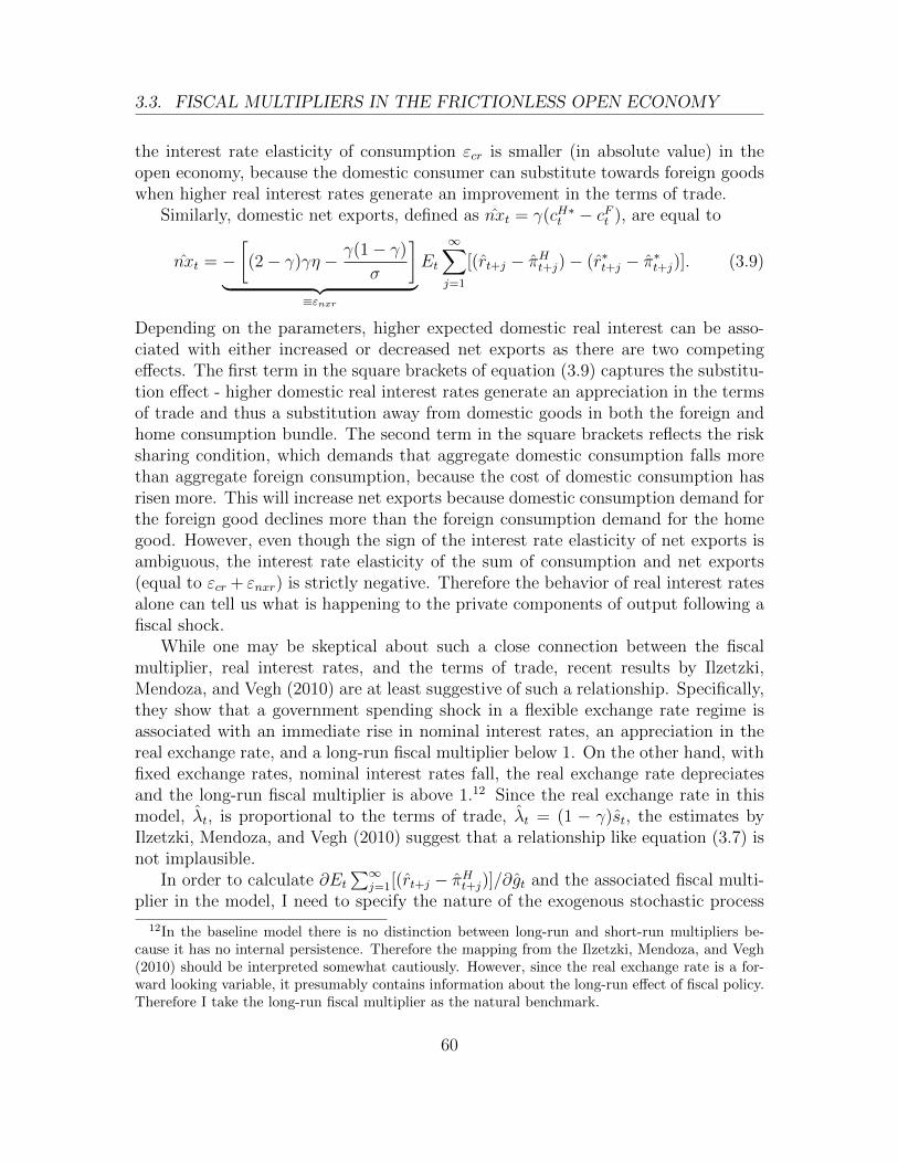
3.3. FISCAL MULTIPLIERS IN THE FRICTIONLESS OPEN ECONOMY
the interest rate elasticity of consumption εcr is smaller (in absolute value) in theopen economy, because the domestic consumer can substitute towards foreign goodswhen higher real interest rates generate an improvement in the terms of trade.
Similarly, domestic net exports, defined as nxt = γ(cH∗t − cFt ), are equal to
nxt = −[(2− γ)γη − γ(1− γ)
σ
]︸ ︷︷ ︸
≡εnxr
Et
∞∑j=1
[(rt+j − πHt+j)− (r∗t+j − π∗t+j)]. (3.9)
Depending on the parameters, higher expected domestic real interest can be asso-ciated with either increased or decreased net exports as there are two competingeffects. The first term in the square brackets of equation (3.9) captures the substitu-tion effect - higher domestic real interest rates generate an appreciation in the termsof trade and thus a substitution away from domestic goods in both the foreign andhome consumption bundle. The second term in the square brackets reflects the risksharing condition, which demands that aggregate domestic consumption falls morethan aggregate foreign consumption, because the cost of domestic consumption hasrisen more. This will increase net exports because domestic consumption demand forthe foreign good declines more than the foreign consumption demand for the homegood. However, even though the sign of the interest rate elasticity of net exports isambiguous, the interest rate elasticity of the sum of consumption and net exports(equal to εcr + εnxr) is strictly negative. Therefore the behavior of real interest ratesalone can tell us what is happening to the private components of output following afiscal shock.
While one may be skeptical about such a close connection between the fiscalmultiplier, real interest rates, and the terms of trade, recent results by Ilzetzki,Mendoza, and Vegh (2010) are at least suggestive of such a relationship. Specifically,they show that a government spending shock in a flexible exchange rate regime isassociated with an immediate rise in nominal interest rates, an appreciation in thereal exchange rate, and a long-run fiscal multiplier below 1. On the other hand, withfixed exchange rates, nominal interest rates fall, the real exchange rate depreciatesand the long-run fiscal multiplier is above 1.12 Since the real exchange rate in thismodel, λt, is proportional to the terms of trade, λt = (1 − γ)st, the estimates byIlzetzki, Mendoza, and Vegh (2010) suggest that a relationship like equation (3.7) isnot implausible.
In order to calculate ∂Et∑∞
j=1[(rt+j − πHt+j)]/∂gt and the associated fiscal multi-plier in the model, I need to specify the nature of the exogenous stochastic process
12In the baseline model there is no distinction between long-run and short-run multipliers be-cause it has no internal persistence. Therefore the mapping from the Ilzetzki, Mendoza, and Vegh(2010) should be interpreted somewhat cautiously. However, since the real exchange rate is a for-ward looking variable, it presumably contains information about the long-run effect of fiscal policy.Therefore I take the long-run fiscal multiplier as the natural benchmark.
60

3.3. FISCAL MULTIPLIERS IN THE FRICTIONLESS OPEN ECONOMY
υt = (gt βt c∗t )′. I assume that the exogenous shocks υt follows a stochastic process as
in Christiano, Eichenbaum, and Rebelo (2011). At time t, υt unexpectedly takes ona positive value, υt > 0 (some elements of υt may still be zeros). At time t+1, and allfuture dates, I assume the following transition probabilities: If at t+ j > t, υt+j > 0,then it remains at this level with probability p, Prob [υt+j+1 = υt+j|υt+j = υt] = p.With probability 1 − p, υt+j+1 = 0, which is an absorbing state. The transitionprobabilities imply that Etυt+j = pjυt.
I outline the solution procedure with this shock process in Appendix B.3. Thisstochastic process is particularly useful because it allows me to derive analytic so-lutions to the fiscal multiplier in and outside the liquidity trap. In particular, thefiscal multiplier in normal times is given by,
µG =(1− p)(1− βp) + κ(φ− p)
(1− p)(1− βp) + κ(φ− p)
1 + (1− sg) νσ [1 + γ(2− γ)(ση − 1)] , (3.10)
and satisfies 0 < µG < 1. The fiscal multiplier in normal times is decreasing inopenness, ∂µG
∂γ< 0, if and only if ση > 1.
If the duration of the liquidity trap remains unchanged, then the fiscal multiplierin the liquidity trap is given by,
µLTG =(1− p)(1− βp)− κp
(1− p)(1− βp)− κp
1 + (1− sg) νσ [1 + γ(2− γ)(ση − 1)] , (3.11)
and satisfies µLTG > 1.13 The fiscal multiplier in the liquidity trap is increasing in
openness,∂µLTG∂γ
> 0, if and only if ση > 1.The intuition behind these results is as follows. An increase in government spend-
ing will initially cause an equal increase in output. As output increases, firms have topay higher wages because of increasing disutility of labor. Since firms’ marginal costincrease, they will pass these costs onto consumers in form of higher prices. Thus, anincrease in government spending raises inflation. In normal times, the central bankwill raise nominal interest rates to fight this inflation. In fact, because of the Taylorprinciple, real interest rates will rise in response to inflation.
According to equation (3.8), higher domestic real interest rates will generate afall in consumption, whereas the effect on net exports (equation (3.9)) depends onthe interest rate elasticity of the terms of trade. However, the sum of domesticconsumption and net exports unambiguously falls. This offsets some of the increasein output due to fiscal policy and explains why the multiplier is less than one.
The condition on σ·η determines how the interest rate elasticity of output changes
13It is easy to show that in a liquidity trap the denominator must be positive. See also Christiano,Eichenbaum, and Rebelo (2011) and Eggertsson (2009).
61

3.4. FISCAL MULTIPLIERS IN FRICTION ECONOMY
with openness (γ).14 In standard calibrations15 ση > 1, which implies that the (ab-solute) interest rate elasticity of net exports rises sufficiently with γ, to compensatefor the reduced interest rate elasticity of domestic consumption. Thus, if ση > 1,then a higher value of γ implies that a given rise in real interest rates will have agreater negative impact on output. Since real interest rates increase following a fiscalshock in normal times, a greater interest rate elasticity of output will imply a lowerfiscal multiplier. Therefore, in normal times, the fiscal multiplier in an open economy(γ > 0) is smaller than in a closed economy (γ = 0).
However, if the economy is in a liquidity trap then nominal interest rates remainfixed at zero. The inflation generated by government spending will then reducereal interest rates. According to equations (3.8) and (3.9), the sum of domesticconsumption and net exports now expands, which amplifies the output response tothe fiscal policy shock and generates a fiscal multiplier above 1. If ση > 1, then theliquidity trap fiscal multiplier in an open economy (γ > 0) is larger than in a closedeconomy (γ = 0), because its interest rate elasticity of output is greater in absolutevalue.
In this example there need not be crowding out of net exports in a liquiditytrap. Indeed, if ση > 1, then the interest rate elasticity of net exports is negativeand there can be crowding in if real interest rates fall. Thus, at the ZLB, theopen economy dimension may actually support fiscal efforts to lift the economy. Ofcourse, if domestic net exports expand then foreign net exports must decline, so thata domestic fiscal expansion may actually reduce foreign output. This would makefiscal expansion in the liquidity trap a beggar-thy-neighbour policy, which will requirea different policy coordination than fiscal expansion in normal times (which is a free-rider problem). In particular, with uncoordinated fiscal policy, countries may expandgovernment spending too much, as they do not internalize the beggar-thy-neighboureffects of fiscal expansion.
3.4 Fiscal Multipliers in friction economy
The results in the preceding section have been derived assuming that UIP holds inthe data, at least conditional on a government spending shock. To see how the resultsmay be sensitive to departures from UIP, consider the exchange rate movements
14This condition is weaker than in Fujiwara and Ueda (2010) who assume η = 1.15For example, Ferrero, Gertler, and Svensson (2008) set σ = 1 and η = 2, while Bodenstein,
Erceg, and Guerrieri (2010a) set σ = 1 and η = 1.5. Obstfeld and Rogoff (2005) argue that η = 2is a reasonable calibration balancing micro and macro estimates. However, they suggest that microestimates (which imply higher elasticities) are likely less biased, and thus also experiment withhigher values of η.
62

3.4. FISCAL MULTIPLIERS IN FRICTION ECONOMY
implied by the model: In normal times the nominal exchange rate appreciates by
∂et∂gt
= − φ− 1
(1− p)(1− γ)
∂πt∂gt
< 0. (3.12)
However, even without any exchange rate response the terms of trade would improvein normal times, and there would have been some crowding out of domestic netexports (for reasonable parameters). This suggests that the qualitative results forthe fiscal multiplier in normal times would still hold, even if the nominal exchangerate fails to appreciate due to limits to arbitrage.
The results are more sensitive in the liquidity trap. In this case the nominalexchange rate depreciates by,
∂et∂gt
=1
(1− p)(1− γ)
∂πt∂gt
> 0, (3.13)
which generates a deterioration in the terms of trade even though domestic prices rise.Suppose that limits to arbitrage prevent the nominal exchange rate from adjustingat all. Then the terms of trade would improve and we would likely see a crowdingout of net exports. This suggests that the fiscal multiplier in the liquidity trap maybe particularly sensitive to departures from UIP.
To investigate this issue more formally, I determine the fiscal multiplier for variousdegrees of friction in the UIP condition. I assume that the friction is proportional tothe excess return on domestic real bonds,
ft =τ
1− p[(rt+1 − EtπHt+1)− (r∗t+1 − EtπF∗t+1)], (3.14)
where τ captures the size of the friction, which is scaled by (1−p) since the expectedfriction also enters the UIP condition. Typically in this model, Etft+1 = pft, andthe UIP condition becomes
Et∆st+1 = (1− τ)[(rt+1 − EtπHt+1)− (r∗t+1 − EtπF∗t+1)]. (3.15)
When τ > 0 the friction will limit the movement of the terms of trade and thus thenominal exchange rate relative to the baseline model. For example, τ = (φ−1)/(φ−p) > 0 corresponds to the case where the nominal exchange rate fails to appreciate innormal times, whereas τ = 1/p > 0 implies that the nominal exchange rate does notdepreciate at the ZLB. The functional form of ft may appear somewhat arbitrary,but since τ will be estimated conditional on it, it is more akin to a convenientnormalization.
The friction τ will affect the fiscal multiplier in two ways. First, by limiting themovement in the nominal exchange rate, it can reduce the effect of fiscal shock on
63

3.4. FISCAL MULTIPLIERS IN FRICTION ECONOMY
net exports, and even switch the sign of the net export response. For example, atthe ZLB when τ = 1/p, the nominal exchange rate is unchanged, so that the termsof trade improve. This will crowd out net exports, whereas in the baseline model(τ = 0) net exports were crowded in. Second, for a given terms of trade response thefriction now allows for a non-proportional consumption response, unlike the baselinemodel. Suppose that the friction is such that the terms of trade response is zerofollowing a government spending shock (τ = 1). If consumption falls (as it does innormal times), then a fraction of it will fall on foreign production, so the multiplierin normal times will be higher. Vice-versa, if consumption rises (as at the ZLB),then the increase in consumption will benefit foreign producers and the domesticfiscal multiplier is smaller. This behavior was absent in the baseline model, becausea zero terms of trade response implied a zero consumption response.
We can see both effects in action by calculating the fiscal multipliers as in section3.3. Incorporating the friction, fiscal multiplier in normal times is now given by,
µFG =(1− p)(1− βp) + κ(φ− p)
(1− p)(1− βp) + κ(φπ − p)
1 + (1− sg) νσ [(1− τγ) + (1− τ)γ(2− γ)(ση − 1)] .
The friction has only affected the last two terms in the denominator: The weight(1 − τ) on the second term reflects the first effect discussed above - by limitingthe change in the terms of trade, net exports become less sensitive to governmentspending. The first term, (1− τγ), captures the second effect noted in the precedingparagraph: When domestic consumption falls, for a given terms of trade response,then this is partly absorbed by net exports. This allows for a higher multiplier innormal times, so long as the import share γ is positive. Note that when γ = 0,we obtain the closed economy fiscal multiplier for all values of τ . Intuitively, netexports are always zero independent of the terms of trade, and consumption is entirelydetermined by domestic real interest rates, for which the friction is irrelevant.
For small to moderate frictions, the results derived in the preceding section alsohold in normal times. In particular, if τ < 1, then the multiplier is less than 1,0 < µFG < 1. In fact, for realistic calibrations of ση and the import share γ, muchlarger frictions can also satisfy this inequality. Thus, the upper bound on the fiscalmultiplier in normal times is quite robust to deviations from UIP. On the otherhand, the comparative static with respect to the import share can be quite sensitiveto τ . In the friction economy, the fiscal multiplier in normal times is decreasing in
openness,∂µFG∂γ
< 0, if ση > 1 and τ < τ = 2(1−γ)(ση−1)/[1+2(1−γ)(ση−1)] < 1.Depending on parameter values this expression can be quite small, although standardcalibrations will put τ in the upper half of the unit interval.
64

3.5. EMPIRICAL STRATEGY & RESULTS
The friction affects the multiplier at the ZLB symmetrically,
µLT,FG =(1− p)(1− βp)− κp
(1− p)(1− βp)− κp
1 + (1− sg) νσ [(1− τγ) + (1− τ)γ(2− γ)(ση − 1)] .
(3.16)where once again µLT,FG > 1 if τ < 1. However, even for larger τ the multiplier willbe above 1 for standard parameterizations. The fiscal multiplier in the liquidity trap
is increasing in openness,∂µLT,FG
∂γ> 0, if ση > 1 and τ < τ < 1. Thus, the friction is
more likely to affect the relative size of open and closed economy fiscal multipliers,rather than the relative size of the fiscal multiplier in normal times and at the ZLB.
3.5 Empirical Strategy & Results
Ultimately, the degree to which UIP fails and its influence on the size and prop-erties of the fiscal multiplier at the ZLB is an empirical question. While ideally onewould like to side track this issue and obtain direct estimates of fiscal multipliersthere is not enough data to use standard empirical tools such as SVARs or estimatedDSGE models. The aim of this paper is thus more modest: obtain estimates of thefriction in UIP and, through the lens of the model, ask if the results obtained in thefrictionless case are robust. In particular, given empirical departures from UIP,
1. is the fiscal multiplier at the ZLB above 1?
2. is the open economy fiscal multiplier at the ZLB larger than the closed economyfiscal multiplier?
To the best of my knowledge this is the first approach that tries to empirically testan aspect of the large fiscal multipliers that obtain in New Keynesian models at theZLB.
There is a long literature that has estimated unconditional departures from UIPby directly estimating equation (3.3) with realized exchange rate data (see e.g. Engel(1996)). However, determining the size of the fiscal multiplier requires knowledge ofthe conditional departures from UIP. In other words, we need to know the sizeof the friction conditional on a government spending shock. Typically conditionaldeviations tend to be smaller than unconditional departures (e.g. Faust, Rogers,Wang, and Wright (2007)), so this distinction can be quantitatively important.
To determine the conditional departures from UIP I examine the nominal ex-change rate response following generic inflationary shocks. If the inflation surprisewas due to a government spending shock, then the nominal exchange rate in thefrictionless model appreciates in normal times as in equation (3.12). As we increase
65

3.5. EMPIRICAL STRATEGY & RESULTS
the friction parameter τ , this appreciation will get smaller and smaller,
∂et∂gt
= −[φ− 1
1− p+ τ
φ− p1− p
]1
1− γ︸ ︷︷ ︸δNT
∂πt∂gt
, (3.17)
and may even turn into a depreciation for large values of τ . Similarly, at the ZLBthe nominal exchange rate depreciates in the frictionless model as in equation (3.13).However, a large enough friction can again switch the sign of the exchange rateresponse,
∂et∂gt
=
[1
1− p− τ p
1− p
]1
1− γ︸ ︷︷ ︸δZLB
∂πt∂gt
. (3.18)
The empirical strategy is to estimate the coefficient δ and, given estimates for φ, γand p, infer the value for τ . I allow the estimate for τ to differ in normal times and atthe ZLB, since the latter period featured more financial turmoil in international assetmarkets. The rest of this section will address some concerns about this empiricalstrategy.
First, it is unlikely that most generic inflation surprises are due to governmentspending shocks. However, equations (3.17) and (3.18) hold for any generic infla-tionary shock in the model, with the exception of ft which I will discuss below. Wecan simply replace gt by some other shock xt 6= ft, which could be either a demandor supply shock, and still use the estimated exchange rate response to determine thefriction parameter τ . I show in Appendix B.5 that the inflation surprises I use appearto be to hitherto unobserved demand shocks. Since there is little a priori reason whyconditional deviations from UIP should vary across different types of demand shocks,using these inflation surprises as proxy is unlikely to considerably bias an estimateof τ .
Second, when ft shocks are a major source of inflation surprises, then this willbias the estimation of τ . In particular, shocks to ft will add a shock to the estimatedexchange rate equation,
∆et = δ∆πt + εt
where εt is the shock to ft, and δ is δNT in normal times (equation (3.17)) or δZLB atthe ZLB (equation (3.18)). The estimated coefficient in this regression will be biaseddepending on the correlation between πt and the shock εt,
E(δ) = δ
(1 +
cov(πt, εt)
var(πt)
).
In the model, cov(πt, εt) ≥ 0 if ση > 1, which implies that ft shocks will bias theestimates δ away from zero and τ downwards. Thus, if the estimated τ is positive,then this is not a consequence of exogenous shocks to the UIP equation.
66

3.5. EMPIRICAL STRATEGY & RESULTS
Third, for a large open economy, there is also some pass-through to inflation ofgoods produced in the foreign country πFt , which will mitigate the movements innominal exchange rate. However, for plausible parameter values this effect is smalland can be ignored: With a domestic import share of γ = 0.15 and a relative size ofthe foreign country of n = 3 (plausible for the US), the foreign import share is justψ = 0.05. This limits the substitution by foreign consumers away or towards foreigngoods, and thus the spill-over from domestic inflation, which is typically less than10% for plausible parameter values. For parameters typical of European countries(γ ≈ 0.3 and n ≥ 9) the pass-through rate is even smaller. I also split the sample intolarge and small open economies and find little difference in the estimated exchangerate responses, suggesting that spill-overs do not bias the estimation.
Fourth, if generic inflation shocks are global then the exchange rate effects willbe very different from those derived above. When both countries face a simultaneousshock to the excess return of their bonds, the effects on the nominal exchange rateare ambiguous. I consider this possibility in to following section, where I show thatinflation surprises in other countries do not forecast current or future inflation in theUS, and thus appear to represent local shocks.
3.5.1 Inflation Surprises
I construct inflation surprises following Clarida and Waldman (2008): The an-nounced inflation values and the associated professional forecasts for inflation arefrom Bloomberg Financial Services. Bloomberg surveys numerous professional fore-casters on their expectations of the next inflation announcement and I take the me-dian of these expectations as the market expectation. The data covers eight countriesfrom February 2000 until January 2010: the US, Great Britain, the Eurozone, Japan,Sweden, Norway, Switzerland, and Canada. For most countries inflation forecastsare available for the CPI and the core CPI. The definitions of the price indices usedare tabulated in Appendix Table B.1 and summary statistics are tabulated in Ap-pendix Table B.2 for headline inflation and appendix Table B.3 for core inflation. Idefine inflation surprises as the difference between the announced and the expectedinflation rate.
Since the empirical test allows inflation surprises, both from demand or supplyshocks, I relegate a more detailed analysis to Appendix B.5 and provide only aninformal summary here. I show that they contain news about current and futuremacroeconomic conditions, and are largely exogenous with respect to past macroe-conomic conditions. However, contemporaneously and over the next two years, infla-tion surprises are associated with higher inflation, lower unemployment and (outsidethe ZLB) higher policy rates. This is consistent with inflation surprises being causedby hitherto unobserved demand shocks, a novel finding to the best of my knowledge.
In addition, neither lagged nor contemporaneous foreign inflation surprises pre-
67

3.5. EMPIRICAL STRATEGY & RESULTS
Table 3.1: Correlation of Inflation Surprise with US Inflation.
Timing: Current Lead Current Lead
Inflation Type: Headline Headline Core Core
Canada 0.330 0.535 -0.0849 -0.245
(0.522) (0.538) (0.223) (0.213)
Switzerland 0.997 1.107
(0.616) (0.659)
Eurozone 1.744 1.238 -0.312 -0.522
(2.370) (2.342) (0.365) (0.367)
Japan 1.804 1.609 -0.0635 -0.209
(1.365) (1.391) (0.310) (0.279)
Norway 0.241 0.0560 0.303 0.292
(0.467) (0.476) (0.233) (0.242)
Sweden 0.263 0.433
(0.652) (0.635)
UK -1.182 -1.274 -0.571∗ -0.590∗
(1.080) (1.150) (0.228) (0.288)
Constant 2.548∗∗∗ 2.543∗∗∗ 2.133∗∗∗ 2.126∗∗∗
(0.139) (0.140) (0.0446) (0.0445)
Observations 109 108 109 108
R2 0.070 0.071 0.042 0.054
F 0.980 1.085 1.491 1.436
p-value 0.450 0.379 0.200 0.218
Standard errors in parentheses, ∗ p < 0.05, ∗∗ p < 0.01, ∗∗∗ p < 0.001
Current = Inflation level in the Month of the Inflation surprise.
Lead = Inflation level in the Month following the Inflation surprise.
68

3.5. EMPIRICAL STRATEGY & RESULTS
dict the inflation levels in the US, the reference country in this analysis. In Table 3.1I regress current US inflation levels on current and lagged foreign inflation surprisesand find p-values that are consistently above 0.2. This suggests that the demandshocks are local in nature, and that have the exchange rate effects described in thepreceding section.
Table 3.2: Persistence of Inflation Surprise in Revised Inflation (Monthly Frequency).
Headline Inflation Core Inflation
AR(1) coefficient 0.930∗∗∗ 0.895∗∗∗
(0.012) (0.020)
Hansen’s J 14.68 15.82
p-value 0.91 0.86
Estimated by GMM. HAC standard errors in parentheses.
∗ p < 0.05, ∗∗ p < 0.01, ∗∗∗ p < 0.001
To infer an estimate of the friction, I need to determine the persistence of theinflation shock. As shown in Appendix B.5, the IRF of inflation to an inflationsurprise is close to an AR(1) process. In Table 3.2, I restrict the impulse to AR(1) ina GMM estimation, which easily satisfies the over-identification restrictions, with p-values of 0.91 and 0.86 respectively. The estimated persistence for headline inflationcorresponds to a value of p = 0.8 at quarterly frequency.
3.5.2 Exchange Rate Response to Inflation Surprises
Next, I examine the exchange rate response to inflation surprises by estimating
∆ei,t = δ0 + δ1πsi,t + δ2LTi,t + δ3LTi,t · πsi,t + εi,t, (3.19)
where ∆ei,t is the change in the natural logarithm of the nominal exchange rate ofcountry i, πsi,t is an inflation surprise,16 and LTi,t is a dummy variable equal to 1 ifthe economy is in a liquidity trap. The estimate of δ1 maps into δNT , while δ1 + δ3
maps into δZLB.
16Inflation that is not a surprise will already be reflected in the exchange rate.
69

3.5. EMPIRICAL STRATEGY & RESULTS
I classify a country to be a liquidity trap at time t as follows. First, I estimatea Taylor rule for all countries except Japan up to the fourth quarter of 2007 (ifavailable). I then use this rule to forecast the predicted unconstrained interest rateup to 2010Q1 and determine in which quarters the predicted rate is below zero.Second, I check if the nominal interest rate in those quarters is the lowest observedin the sample, so that there is no more room for the central bank to cut rates givenits implicit interest rate floor. If a quarter satisfies both conditions then I set theliquidity trap dummy for that quarter equal to 1. The details of the estimationprocedure are relegated to Appendix B.7. For Japan the zero bound constraint isbinding too frequently in the sample to estimate a Taylor rule. I therefore defineJapan to be in a liquidity trap, whenever its policy rate is less than or equal to 0.25.
The exchange rate changes ∆ei,t are high-frequency as in Clarida and Waldman(2008). For each inflation announcement from January 2005 until January 2010 Icalculate the percentage change of the exchange rate against the US Dollar from 5minutes before the announcement to 5 minutes after the announcement.17,18 I tabu-late summary statistics for the percentage change in the exchange rate in AppendixTable B.4. All exchange rates are expressed in terms of units of foreign currency soa negative percentage change corresponds to an appreciation (as in the model).
Since equation (3.19) is non-structural it may be helpful to provide some inter-pretation on its form. First, it is not necessary to include inflation announcements ofthe foreign country in equation (3.19). Inflation announcements are made at differenttimes across countries so whenever πsi,t 6= 0, then for all other countries j 6= i, πsj,t,within the 10-minute window that I consider. Thus, equation (3.19) will yield thesame result as if I was controlling for foreign inflation surprises within the 10-minutewindow.
Second, it is not necessary to control if the foreign country is in a liquidity trap ornot. Within the small open economy model of section 3.3 the exchange rate responsewill be the same irrespective of the foreign state. Intuitively, the domestic inflationsurprise does not spill over to the large foreign country, so there is no foreign interestrate response even if the foreign country was unconstrained. For plausible parametersof a large open economy such as the US, the spill-overs in a calibrated model are alsosmall. Nevertheless, as one robustness check I limit the estimation to small openeconomies.
I estimate equation (3.19) as a pooled regression with bootstrapped standarderrors corrected for the presence of estimated regressors. The estimates are tabulatedin Table 3.3. The first column contains the regression using year-on-year headlineinflation surprises. Accordingly, in normal times a one percent inflation surprise isassociated with a 0.876% appreciation of the home currency. The standard error of
17The data was supplied by Olsen Data and is recorded at 5-minute frequency.18I use the British Pound as a reference currency for the US Dollar.
70

3.5. EMPIRICAL STRATEGY & RESULTS
this estimate is 0.189, so the estimate is statistically significant at the 1% level. Withp = 0.8, γ = 0.15 and φ = 1.5 this estimate implies a moderate friction in normaltimes, τ = 0.50. Higher values for the import share do not affect his estimate verymuch, e.g. setting γ = 0.3 yields τ = 0.54.
The estimates for δ1 are very stable across the robustness checks I consider: Incolumn (2) I add country and time fixed effects, in column (3) I restrict the sample tosmall open economies (excluding the US and the Eurozone), in column (4) I excludeJapan, and in column (5) I use core inflation surprises instead of headline inflationsurprises. The estimate for δ1 ranges from -0.84 to -0.93 and is always significant atthe 1% level. This result confirms earlier estimates by Clarida and Waldman (2008),who find that a 1% point (quarterly) surprise inflation generates a 0.6% appreciationin the nominal exchange rate in a set of 10 countries using data from July 2001 untilDecember 2005.19 The implied range for τ is correspondingly tight - it ranges from0.48 to 0.51 across these estimates.
Turning now to the estimates for the liquidity trap, I tabulate the total exchangerate response (the sum of the first row and the third row) along with the standarderror in the two bottom rows of Table 3.3. Accordingly, the exchange rate appreciatesby 0.063% for each percentage point of the inflation surprise, with a standard errorof 0.366. This is significantly different from the exchange rate response outsidethe liquidity trap at the 10% level. However, the frictionless model predicted adepreciation in the domestic currency, which suggests that the friction to UIP musthave been particularly large at the ZLB. In fact, with p = 0.8 and γ = 0.15 I obtainan estimate of τ = 1.26, which is significantly larger than in normal times. Thisestimate is even less sensitive to the choice of γ than the estimate for normal times.
The robustness checks yield similar results, although less precisely estimated thanδ1. Reading across columns (1) through (5) in Table 3.3, the estimate ranges from-0.01 (column (5)) to -0.23 (column (4)). In all cases I can reject the hypothesisthat the domestic currency depreciates as predicted by the frictionless model. Theimplied range of τ for the ZLB estimates is 1.25 to 1.30.
The results are unlikely to be driven by measurement error: First, inflation sur-prises are followed by significant movements in macroeconomic aggregates, whichsuggests that they do contain useful information about shocks (see Appendix B.5).Second, the estimates at the ZLB would have been even more negative if there is
19Nevertheless, the implied appreciation in the real exchange rate contrasts with growing lit-erature, which estimates real exchange depreciations following fiscal shocks (Corsetti, Meier, andMuller (2009); Monacelli and Perotti (2010); Ravn, Schmitt-Grohe, and Uribe (2007)). However,Ilzetzki, Mendoza, and Vegh (2010) find that the real exchange rate appreciates following a fiscalshock for countries with flexible exchange rates. Furthermore, in robustness checks by Corsetti,Meier, and Muller (2009) the real exchange rate appreciates if fiscal shocks are identified using theRamey and Shapiro (1998) dates. Thus, a real exchange rate appreciation following a fiscal shocksdoes not appear to be implausible.
71

3.5. EMPIRICAL STRATEGY & RESULTS
Table 3.3: Exchange Rate Response to Inflation Surprises
Inflation Measure Headline Inflation Core
All Country SOE Excl. All
Countries &Time only Japan Countries
Pooled FE Pooled
(1) (2) (3) (4) (5)
Surprise Inflation (δ1) -0.867∗∗∗ -0.831∗∗∗ -0.936∗∗∗ -0.915∗∗∗ -0.861∗∗∗
(0.189) (0.165) (0.214) (0.195) (0.246)
Liquidity Trap (δ2) -0.012 0.147 -0.027 0.015 -0.027
cle (0.045) (0.087) (0.054) (0.054) (0.051)
Inflation-Liquidity 0.804∗ 0.675∗ 0.741 0.690 0.852
Trap Interaction (δ3) (0.417) (0.366) (0.519) (0.486) (0.543)
Country & Time FE No Yes No No No
Observations 485 485 363 426 356
R2 0.107 0.279 0.279 0.126 0.072
δ1 + δ3 -0.063 -0.156 -0.195 -0.225 -0.009
(0.366) (0.330) (0.471) (0.441) (0.479)
Bootstrapped standard errors in parentheses, ∗ p < 0.1, ∗∗ p < 0.05, ∗∗∗ p < 0.01
All regressions use CPI non-flash inflation announcements.
72

3.6. QUANTITATIVE ANALYSIS
bias towards zero, which would imply an even greater distortion to UIP. Therefore,measurement error in the data cannot explain the discrepancy between the estimatesand the predictions of the frictionless baseline model.
3.6 Quantitative analysis
Given estimates for τ in normal times and at the ZLB, I can calibrate the modelto assess the quantitative and qualitative importance of departures from UIP. I cali-brate the model with a set of standard parameters, which largely follow Christiano,Eichenbaum, and Rebelo (2011) and Bodenstein, Erceg, and Guerrieri (2009). Thediscount factor β is calibrated at 0.99 to match an average real interest rate of 4% peryear. The inverse Frisch elasticity ν is set to 0.5 and the IES σ−1 is set to 1 to allowfor sufficient output variation in a model without capital. The share of governmentin output sg is set to 0.2 and the import elasticity η to 2 as suggested by Obstfeldand Rogoff (2005). The Calvo probability θ is calibrated at 0.85 to accord with thesmall inflation response in this recession.20 The persistence of the shock is set top = 0.8 as estimated in Section 3.5.1.
In Figure 3.1 I display the baseline fiscal multiplier in normal times and at theZLB, as well as the multipliers in the friction model while varying the import shareγ from 0 to 0.5. As proven in section 3.3, in the baseline model the fiscal multiplieris less than 1 and decreasing in the import share in normal times, while it is greaterthan 1 and increasing in the import share at the ZLB. The estimated friction barelyaffects the multiplier much in normal times - it is still less than 1 and decreasing inthe import share. In fact, even much larger frictions, such as those estimated duringthe ZLB, will not push the fiscal multiplier above 1 during normal times. Smallfiscal multipliers appear to be a robust feature during normal times, irrespective ofweather UIP holds or not.
The same cannot be said for the ZLB. For small import shares as in the US(γ = 0.15), the fiscal multiplier in the friction model is “only” 1.5, whereas it assumesa value of 2.5 in the baseline model. Nevertheless, it is above 1 and it would requirean extremely large friction - τ = 3.5 - to push the multiplier below 1 for theseparameters. However, unlike the baseline model the multiplier in the friction modelis now decreasing in γ. The resulting difference between the closed economy fiscalmultiplier and the friction multiplier are quantitatively significant, particularly atimport shares relevant for European countries. For example, with γ = 0.3 thefriction multiplier is 30% smaller than the closed economy fiscal multiplier. Thissuggests that for empirically relevant departures from UIP, exchange rate crowding
20This calibration is equivalent to a model with firm-specific labor, where the Calvo probabilityis set to θ = 0.7 (as suggested by Nakamura and Steinsson (2008)) and the elasticity of substitutionacross goods equals ε = 10.
73

3.6. QUANTITATIVE ANALYSIS
Figure 3.1: Fiscal multipliers for the baseline and friction model in normal times andat the ZLB.
0 0.1 0.2 0.3 0.4 0.50
0.5
1
1.5
2
2.5
3
3.5
4
Import share γ
Fis
ca
l M
ultip
lier
Baseline Model: Normal Times
Friction Model: Normal Times
Baseline Model: ZLB
Friction Model: ZLB
74

3.6. QUANTITATIVE ANALYSIS
out can be quantitatively important even at the ZLB.
3.6.1 A model with capital
In this section I add capital to the model to check the robustness of the resultsin the previous section. I allow capital to be completely mobile across firms, thathave Cobb-Douglas technology with capital share α. Aggregate capital depreciates at
rate δ and is accumulated subject to a quadratic adjustment cost ψ2
(It
Kt−1− δ)2
Kt−1,
where Kt is capital and It is investment. Investment goods are produced using thesame weights on domestic and foreign goods as consumption in the baseline model,
it = (1− γ)iHt + γiFt (3.20)
and with elasticity of substitution η between home and foreign goods. Allowing forcapital results in two new (log-linearized) first order conditions, an Euler equationfor capital,
ct = Etct+1 −1
σ
[βR(1− α)(nt+1 − kt) + βqt+1 − qt + βt+1
](3.21)
and an equation for Tobin’s q,
qt = ψ(kt − kt−1) (3.22)
This model can no longer be solved analytically for the fiscal multiplier, so I solve thismodel using the algorithm from Bodenstein, Erceg, and Guerrieri (2009). Coibion,Gorodnichenko, and Wieland (2011) show that this algorithm remains accurate evenfor large shocks that will push the economy to the ZLB. To make the estimatescomparable to the baseline model, I let the ZLB bind for 5 quarters. I set the capitalshare α = 0.33, the depreciation rate at δ = 0.02 and the investment adjustment costat ψ = 7 as in Shapiro (1986). In addition the Frisch elasticity of labor supply ν−1 isreduced to 2/3, and the IES σ−1 to 0.5, since investment will now induce sufficientoutput variability.
Importantly, introducing capital does not invalidate the empirical analysis insection 3.5, as the friction enters the UIP relationship in exactly the same fashion.Thus, the same estimated friction can be used to calibrate the model with capital.21
The fiscal multipliers for the capital model, as well as the capital model with frictionare reported in Figure 3.2.
Adding capital does not change the qualitative behavior of fiscal multipliers innormal times: They are small, less than 0.5, both in the standard model and the
21Because the persistence of inflation is endogenous in the capital model I adjust p in equation(3.14) to hit the estimated exchange rate response in Table 3.3.
75

3.6. QUANTITATIVE ANALYSIS
Figure 3.2: Fiscal multipliers for the capital model.
0 0.1 0.2 0.3 0.4 0.50
0.5
1
1.5
2
2.5
3
3.5
4
Import share γ
Fis
ca
l M
ultip
lier
Capital Model: Normal Times
Capital Model with Friction: Normal Times
Capital Model: ZLB
Capital Model with Friction: ZLB
The fiscal multipliers are calculated for normal times, binding ZLB, normal timeswith friction, and binding ZLB with friction.
76

3.7. CONCLUSION
model with friction. More action occurs at the ZLB: Here, the fiscal multiplier isincreasing in the import share in the baseline model with capital, but this is reversedwhen I add the friction to international asset markets. The differences between thebaseline multiplier and the friction multiplier are smaller than in the model withoutcapital, but still quantitatively significant. Furthermore, letting γ = 0.3 in thefriction model again reduces the fiscal multiplier by about 30% relative to the closedeconomy, which confirms the earlier finding that exchange rate crowding out canbe quantitatively important. Finally, the friction fiscal multipliers remain above 1for reasonable import shares, and are significantly larger than fiscal multipliers innormal times.
In summary, incorporating the empirically estimated friction into the standardmodels significantly affects the properties of the fiscal multiplier at the ZLB. It will besmaller in the open economy than in the closed economy, because the friction preventsfavorable exchange rate adjustments that occur in the baseline model. However, ittypically remains above 1, which is large by the standards of the economy literature.This suggests that fiscal policy in the open economy is effective at the ZLB, althoughnot as much as our baseline models may lead us to believe.
3.7 Conclusion
In this paper I have provided both theory and evidence on the open economyfiscal multiplier in a liquidity trap. I show that in open economy New Keynesianmodels, the fiscal multiplier at the ZLB is greater than 1 and increasing in theimport share if there are no frictions to international asset markets. Intuitively, theopen economy’s interest rate sensitivity of output is greater (in absolute value), sothat it gets a larger boost from a given decline in real interest rates. Indeed, forstandard parameterization, the home countries’ net exports rise, so that domesticfiscal expansion in the liquidity trap has a beggar-thy-neighbour effect.
I then show that sufficiently large frictions in international asset markets thatmanifest themselves as departures from UIP, can overturn both conclusions. In thiscase, a large friction will prevent the nominal exchange rate depreciation that occursin the baseline model, so that the terms of trade improve. This can crowd out netexports sufficiently such that the open economy has a smaller multiplier than theclosed economy, and that this multiplier is below 1.
To distinguish between these conflicting predictions and determine the likelyproperties of the open economy fiscal multiplier at the ZLB, I estimate the sizeof the friction by examining the exchange rate response to generic inflation surprises.While the frictionless model predicts that the nominal exchange rate depreciates bymore than 1% for each 1% point of inflation at the ZLB, I estimate essentially a zeroresponse. Thus, large frictions are needed to rationalize this exchange rate response.
77

3.7. CONCLUSION
A model calibrated with the estimated friction shows quantitatively importantdeviations from the baseline model at the ZLB. The fiscal multipliers are significantlysmaller, even at moderate import shares, and decline as the import share rises.Nevertheless, the fiscal multipliers in the friction model are typically above 1, whichis large given the standards of an open economy (e.g. Dornbusch (1976), Ilzetzki,Mendoza, and Vegh (2010)).
As more data on ZLB episodes becomes available, more empirical work will berequired to sharpen our estimates of the fiscal multiplier in the current economicenvironment. In the meantime, as we resort to model-based analysis, the results ofthis paper suggest that frictions in international asset markets can have importantquantitative implications for the open economy fiscal multiplier, particularly at theZLB. Evidently, more research is needed to understand the sources of these frictionsand their connections to the real economy.
78

Chapter 4
Are Negative Supply ShocksExpansionary at the ZLB?
“As some of us keep trying to point out, the United States is in a liquiditytrap: [...] This puts us in a world of topsy-turvy, in which many of theusual rules of economics cease to hold. Thrift leads to lower investment;wage cuts reduce employment; even higher productivity can be a bad thing.And the broken windows fallacy ceases to be a fallacy: something thatforces firms to replace capital, even if that something seemingly makesthem poorer, can stimulate spending and raise employment.”
Paul Krugman, 3rd September 2011.
4.1 Introduction
The preceding chapter has highlighted that government spending at the ZLBcan be very effective. This has lead some economists to argue that demand-side poli-cies, such as fiscal stimulus and forward guidance, are well-suited to address the ZLBproblem (e.g., Bernanke (2012), Eggertsson and Krugman (2011), Woodford (2012)).However, these strong expansionary effects arise because such policies increases pro-duction costs, which raises inflation expectations through the Phillips curve (1.2),lowers real interest rates and stimulates consumption. Thus, implicit in this argu-ment is that negative supply shocks, i.e. shocks that raise inflation expectations, areexpansionary through the inflation expectations channel. As a result, opponents areskeptical whether these models, originally designed and estimated to match normaltimes, describe the ZLB accurately enough to justify such bold policy choices (e.g.,Cochrane (2009), Taylor (2012)).
This chapter contributes to this debate in three ways. First, using a variety of
79

4.1. INTRODUCTION
empirical tests I reject the prediction that negative supply shocks are expansionary atthe ZLB. Second, I show that incorporating credit frictions into sticky-price models isimportant to match this stylized fact. However, this necessity only becomes clear atthe ZLB when the central bank’s stabilization policy no longer dampens the financialaccelerator. Third, I demonstrate that fiscal policy and forward guidance at theZLB are significantly less effective in the model with credit friction than in standardsticky-price models, and that this is a robust feature of models where negative supplyshocks are contractionary at the ZLB. Thus, contrary to Krugman’s assertion, thebehavior of the ZLB economy can be quite similar to that in normal times.
Standard new Keynesian models emphasize the importance of expectations inthe propagation of shocks. With a standard Euler equation, consumption today isdetermined by expected future real interest rates and expected long-run consump-tion. Temporary, negative supply shocks do not affect long-run consumption, butraise inflation expectations when prices are sticky. In normal times (i.e., outside theZLB), the central bank raises nominal interest rates enough that expected real inter-est rates rise (the Taylor principle) and consumption contracts. In contrast, nominalinterest rates remain unchanged when the central bank is constrained by the ZLB, sothat higher inflation expectations reduce real interest rates and consumption todayexpands. I call this mechanism the “expectations channel,” since inflation expec-tations are the key quantity through which supply shocks affect real output at theZLB.
In my first contribution, I test for the inflation expectations channel by examiningtwo types of evidence. First, I determine the macroeconomic impact of two negativesupply shocks at the ZLB: oil supply shocks, and the Japanese earthquake in 2011.My results show that while inflation expectations rise and expected real interest ratesfall as predicted by the theory, these negative supply shocks are still contractionaryoverall. I also provide evidence against a weaker interpretation of the expectationschannel. Because expected future nominal rates rise less at the ZLB, supply shocksshould be less contractionary than in normal times; however, I document that oilsupply shocks appear to be, if anything, more contractionary at the ZLB. Thissuggests that the expectations channel plays only a limited role in the propagationof such shocks. To the best of my knowledge, this is the first paper to test directly forthe expansionary effects of negative supply shocks through the expectations channelat the ZLB.
Second, I argue that inflation risk premia can signal if generic negative supplyshocks are also contractionary at the ZLB. In standard models, higher expectedinflation raises consumption at the ZLB irrespective of its source, so nominal assetsbecome a hedge — they gain value in deflationary states when consumption is low.Conditional on the ZLB, the inflation risk premium should therefore be negative.However, empirically the one-year inflation risk premium at the ZLB is typicallypositive, suggesting that investors want to insure against shocks that raise inflation
80

4.1. INTRODUCTION
and lower consumption. This indicates that generic negative supply shocks are notonly contractionary at the ZLB, but also a significant contributor to inflation riskover this horizon.
These findings constitute a puzzle for any model with a standard Euler equation,since it predicts that consumption should expand given the lower real interest ratesin the data. As my second contribution, I show that incorporating financial frictionsin the Euler equation reconciles the theory with the data.1 Following Gertler andKiyotaki (2010) and Curdia and Woodford (2009), my model features a balancesheet constraint on financial intermediaries that generates an endogenous spreadbetween the borrowing and the deposit rate. Because a negative supply shock reducesprofits and share values, the net worth of financial intermediaries falls, tighteningtheir balance sheet constraints. In turn, banks contract loan supply, the borrowingspread rises, and borrowers reduce consumption such that negative supply shocksare contractionary at the ZLB.
While my model is more successful at matching the data, in normal times it be-haves similarly to a standard new Keynesian model. Intuitively, the central bankresponds more aggressively to amplified inflation and output responses, which en-dogenously dampens the financial accelerator. This suggests that differences betweenmodels are “smoothed-out” in normal times, allowing a variety of models to matchthese kinds of data. Since this mechanism is absent at the ZLB, many such modelswill be less successful at matching these data, even if they worked well in normaltimes. On the flip-side, the ZLB provides a unique testing ground, because one canmore easily discriminate among models when propagation mechanisms are uninhib-ited by central bank actions.
As my third contribution, I show that demand-side policies at the ZLB are lesseffective in models that match these data. For instance, in a new Keynesian modela government spending shock at the ZLB raises current and expected marginal cost,which increases expected inflation, lowers real interest rates, and stimulates con-sumption so that the fiscal multiplier exceeds one. Thus, ZLB multipliers are largebecause higher marginal costs raise consumption through the expectations channel— but this prediction is rejected in the data! In any data-consistent model the risein inflation expectations from higher marginal costs cannot be expansionary, so thatfiscal policy becomes much less effective. Consequently, in the calibrated model withcredit frictions, demand-side policies are up to 50% less effective than in a stan-dard new Keynesian model. This suggests that policy makers should be cautious inexpecting large positive outcomes from such policies at the ZLB.
This paper is closely related to literature that has explored how standard macroe-conomic models make very different, even paradoxical, predictions at the ZLB. My
1In Section 4.5, I discuss the reasons for this modeling choice as well as other (complementary)mechanisms.
81

4.1. INTRODUCTION
empirical results concern primarily the “Paradox of Toil:” Eggertsson (2010b, 2011,2012) showed how standard new Keynesian models robustly predict that negativesupply shocks (e.g., greater monopoly power, higher labor taxes) are expansionaryat the ZLB through the expectations channel. As such, increases in desired laborsupply (a positive supply shock) become self-defeating, because the resulting defla-tion reduces demand and equilibrium employment. In addition, according to the“Paradox of Thrift” a rise in the desire to save is also self-defeating at the ZLB, be-cause it reduces output so much that aggregate savings fall (Keynes (1936), Krugman(1998), Eggertsson and Woodford (2003), and Christiano (2004)). Finally, accordingto the “Paradox of Flexibility,” output volatility may rise at the ZLB if prices andwages become more flexible (e.g., Werning (2011), Eggertsson and Krugman (2011)).
Empirical validations of these paradoxes are scarce. In a first examination of the“Paradox of Toil,” Mulligan (2010, 2012) argues that seasonal labor inflows do notappear contractionary and higher minimum wages do not appear expansionary inthe data. However, Eggertsson (2010a) disputes that these tests are valid becausethe shocks are either forecastable or permanent, and therefore cannot raise inflationexpectations and work through the expectations channel. Second, Bachmann, Berg,and Sims (2011) show that consumers with above-average inflation expectations,i.e. below average expected real interest rates, have lower willingness to spend.However, in their cross-sectional analysis they cannot test whether aggregate inflationexpectations are expansionary at the ZLB as predicted by the expectations channel.My analysis is robust to these critiques, as the supply shocks I use raise aggregateinflation expectations and lower expected real interest, yet still are contractionary.
This stylized fact has important implications for the literature on fiscal multi-pliers. There is an ongoing debate whether fiscal multipliers are large at the ZLB(e.g., Christiano, Eichenbaum, and Rebelo (2011); Woodford (2011a)) or small (e.g.,Cogan, Cwik, Taylor, and Wieland (2010); Drautzburg and Uhlig (2011)). This pa-per shows that when negative supply shocks are contractionary at the ZLB, thenthe inflation expectations channel cannot be a source of large multipliers. To theextent that multipliers may be large at the ZLB, my results suggest that these aredue to other mechanisms such as consumption-labor complementarities (Nakamuraand Steinsson (2011)), low capacity utilization (Christiano, Eichenbaum, and Rebelo(2011)), or high unemployment (Michaillat (2012)).
This paper proceeds as follows. In Section 4.2, I show that temporary, negativesupply shocks are expansionary in standard sticky-price models when the ZLB binds.In Section 4.3, I reject this prediction for oil supply shocks and an earthquake. InSection 4.4, I calculate one-year inflation risk premia to determine if generic negativesupply shocks are also contractionary at the ZLB. In Section 4.5, I build a model withcredit frictions that can match these facts, and in Section 4.6 I derive implicationsfor demand-side policies. I conclude in Section 4.7.
82

4.2. PREDICTIONS FROM STANDARD STICKY-PRICE MODELS
4.2 Predictions from Standard Sticky-Price
Models
I derive predictions in the continuous-time adaptation of a standard new Key-nesian model from Woodford (2003).2 In Appendix A.2, I illustrate how the moreelaborate Smets and Wouters (2007) model also predicts that negative supply shocksare expansionary at the ZLB. Eggertsson (2012) shows further robustness of thisprediction in a number of extensions.
Consider a representative agent with separable utility U(t) = C(t)1−γ−1−1
1−γ−1 − L(t)1+ν
1+ν,
where C(t) is the consumption flow, L(t) is labor supply, γ is the intertemporalelasticity of substitution, and ν is the inverse Frisch elasticity. This agent can hold arisk-free nominal bond that pays an instantaneous nominal interest rate i(t), as wellas a complete set of Arrow-Debreu securities. The optimal allocation must satisfythe standard Euler equation,
Et[d lnC(t)] = γ[i(t)− π(t)− %− v(t)]dt, (4.1)
where π(t) is the instantaneous inflation rate, % the instantaneous discount rate, andv(t) is an exogenous demand shifter.
Solving the Euler equation forward illustrates that today’s consumption dependson the sum of expected real interest rates and expected consumption in the far future:
lnC(t) = −γEt∫ ∞
0
[i(t+ s)− π(t+ s)︸ ︷︷ ︸Expected Real Rates
−%− v(t+ s)]ds+ Et limT→∞
lnC(T )︸ ︷︷ ︸“Long-Run” Consumption
. (4.2)
Thus, consumption today is high relative to the long-run consumption level if theexpected path of real interest rates is relatively low, and vice-versa.
I assume that the supply side of the model is given by a standard new KeynesianPhillips curve,
dπ(t) = %π(t)− κ[(γ−1 + ν)(lnC(t)− lnC) + (1 + ν)u(t)] (4.3)
where lnC = Et limT→∞ lnC(T ) is the expected long-run consumption level andu(t) is a temporary, negative supply shifter (e.g., a temporary, negative technologyshock).
2Braun, Korber, and Waki (2012) demonstrate that the log-linear approximations used herecan become inaccurate at the ZLB, and that negative supply shocks may be contractionary in thetrue non-linear model. However, Christiano and Eichenbaum (2012) argue that the approximationsremain valid if output deviates by less than 20% from steady-state as is the case in my calibration.In addition, my findings in Sections 4.2 and 4.3 remain a puzzle in Braun, Korber, and Waki (2012),because even in the non-linear model lower real interest rates should stimulate consumption andthe inflation risk premium should be negative.
83

4.2. PREDICTIONS FROM STANDARD STICKY-PRICE MODELS
This paper employs the new Keynesian Phillips curve merely as a convenient wayto introduce price stickiness. For the purpose of this analysis the key property ofEquation (4.3) is that a temporary, negative supply shock raises expected inflation —a prediction that is verified in the empirical analysis below. This property is sharedby other sticky-price models (e.g., Taylor (1979)), and this paper does not take astand on the relative merits of these settings. However, this prediction contrasts withflexible-price economies where temporary, negative supply shocks trigger expecteddeflation, because firms immediately raise prices and then let them gradually fall asthe supply shock dissipates.
To analyze the effect of a negative supply shock I first differentiate Equation(4.2),
d lnC(t)
du(t)= −γ
dEt∫∞
0[i(t+ s)− π(t+ s)]ds
du(t)+
dEt limT→∞CTdu(t)
.
This reveals that the supply shock can affect consumption by changing either realinterest rates or long-run consumption. I restrict my attention to persistent, buttemporary supply shocks, so that the second term on the right-hand side (RHS) iszero. Thus, a temporary, negative supply shock can be expansionary if and only ifit lowers the expected sum of future real interest rates — the first term on the RHS.
Summary 2 Given the Euler equation (4.1), a temporary, negative supply shock —an increase in u(t)— is expansionary if and only if it lowers the sum of expected realinterest rates:
dEt∫∞
0[i(t+ s)− π(t+ s)]ds
du(t)< 0.
A crucial determinant of the real interest rate response is the interest rate rule ofthe central bank. I assume that it takes a standard linear form subject to the ZLB,
i(t) = maxi+ φππ(t) + φy(lnC(t)− lnC), 0. (4.4)
This rule encompasses inflation targeting as a special case (φπ → ∞), which is thetime-consistent optimal policy rule in this setting.
Suppose that the supply shifter u(t) follows a Poisson process as in Eggertssonand Woodford (2003). This stochastic process is popular because it is convenient foranalyzing the ZLB, but other stochastic processes yield similar results (e.g., Farhiand Werning (2012a)). Initially, the economy is subject to an unanticipated negativesupply shock, u(0) = u > 0, and u(t) subsequently evolves according to
du(t) = −udN(t), dN(t) =
1 with prob. λdt if N(t) = 0
0with prob. 1− λdt if N(t) = 0
with prob. 1 if N(t) = 1
84

4.2. PREDICTIONS FROM STANDARD STICKY-PRICE MODELS
where N(0) = 0. In other words, the system originally starts in the state s(0) =u(0) = u, N(0) = 0, and then stochastically reverts to the absorbing state s =u(t) = 0, N(t) = 1. Thus, the supply shock ceases with probability λdt over aninterval dt. In Appendix A.1, I formally solve the system of differential equations,whereas this section proceeds with a more intuitive discussion of the results.
Suppose first that the ZLB does not bind. Then the economy is split in tworegimes — while the supply shock is active lnC(t) and π(t) are a constant functionof u(t) = u > 0, whereas if the supply shock has ceased the economy returns tosteady-state where lnC(t) = lnC and π(t) = 0. Therefore, conditional on thefirst regime, Etd lnC(t) = −λC(t)dt, which I substitute into the Euler equation todetermine the impact of the supply shock
d lnC(t)
du= −γ (φπ − 1)
λ
dπ(t)
du− γφy
λ
d lnC(t)
du. (4.5)
The terms on the RHS are respectively the change in real interest rates from higherinflation and from movements in consumption. Conditional on a supply shock, Equa-tion (4.5) traces out a downward-sloping line in the (lnC(t), π(t))-space with sloped lnC(t)
dπ(t)= − φπ−1
λ+γφy, which is plotted in Figure 4.2(a). Intuitively, under the policy rule
(4.4) higher expected inflation from a supply shock translates into higher expectedreal interest rates, which reduces consumption today. Since this curve is derived fromthe consumer’s FOC, I label it the “Aggregate Demand” (AD) curve as is commonin the literature (e.g., Romer (2011)).
Using the supply side (4.3), I substitute dπ(t)du
= κ(γ−1+ν)λ+%
d lnC(t)du
+ κ(1+ν)λ+%
and obtain
that a negative supply shock (an increase in u) lowers consumption in normal times
d lnC(t)
du=
−κγ(φπ − 1)(1 + ν)
(λ+ γφy)(%+ λ) + (φπ − 1)κ(1 + γν)< 0.
This is illustrated in Figure 4.2(a), which plots the supply side (4.3) as an upward-sloping AS curve, because higher consumption triggers higher expected inflation byraising marginal costs. A negative supply shock raises expected and actual inflationceteris paribus, so that the AS curve shifts up to AS2. The central bank respondsby raising real interest rates, so that consumption contracts. Thus, consistent withSummary 2, negative supply shocks are contractionary in normal times because theyraise expected real interest rates.
While in normal times the central bank raises nominal interest rates enough toalso raise real rates, this may not occur when the central bank is constrained bythe ZLB. For example, if a negative supply shock raises the shadow nominal interestrate from −3% to −2%, then the actual nominal interest rate remains zero. To focuson this case, I follow Eggertsson and Woodford (2003) and introduce a negativedemand shock that makes the ZLB bind. In particular, I let v(0) = −v < 0 and
85

4.2. PREDICTIONS FROM STANDARD STICKY-PRICE MODELS
dv(t) = vdN(t). This splits the economy in a ZLB and a non-ZLB regime, and thesupply shock only affects the economy in the ZLB state.
At the ZLB, the Euler equation then yields
d lnC(t)
du= γ
1
λ
dπ(t)
du⇒ d lnC(t)
dπ(t)= γ
1
λ> 0. (4.6)
Compared to aggregate demand in normal times (Equation (4.5)) the persistence ofinflation λ enters analogously. However, there is no change in nominal interest ratesso that the terms involving the policy parameters φπ and φy drop out. The resultingAD curve is now upward-sloping, as shown in Figure 4.2(b), because at the ZLBhigher expected inflation lowers expected real interest rates so that consumptionexpands. The upward-shift in the AS curve from a negative supply shock thereforeraises consumption,
d lnC(t)
du=
κγ(1 + ν)
λ(%+ λ)− κ(1 + γν)> 0,
because — consistent with Summary 2 — expected real interest rates fall. As shownin Appendix A.1, determinacy at the ZLB requires that the denominator is positive,which implies that the AD curve is steeper than the AS curve in Figure 4.2(b).3
Summary 3 Consider an economy that satisfies the Euler equation (4.1), the supplyside (4.3), and let monetary policy be given by (4.4). Then, a temporary, negativesupply shock — an increase in u(t) — that does not persist after the ZLB binds isexpansionary because it lowers expected real interest rates.
The previous stochastic process implies that the supply shock does not affect theeconomy after the ZLB ceases to bind. However, if a negative supply shock persistsbeyond the duration of the ZLB, then the central bank may raise real interest ratesat those dates, which will impact today’s consumption through the Euler equation.I call these effects “spillovers.” For example, if exit from the ZLB is governed by anexogenous Poisson process with intensity λZLB, then the change in real interest ratesis given by
dEt∫∞
0[i(t+ s)− π(t+ s)]ds
du(t)=−
dEt∫∞
0[π(t+ s)]ds
du(t)︸ ︷︷ ︸<0 (supply shock raises inflation)
+dEt
∫∞0
(1− e−λZLBs)[i(t+ s)]ds
du(t)︸ ︷︷ ︸Exit from ZLB: Spillovers
.
3In important, recent work Aruoba and Schorfheide (2012), Braun, Korber, and Waki (2012),and Mertens and Ravn (2013) analyze the properties of an economy in the indeterminacy region.I focus on the determinacy case, because in that region a negative supply shock raises expectedinflation and lowers expected real interest rates as is empirically the case in Section 4.3.
86

4.3. NEGATIVE SUPPLY SHOCKS AT THE ZLB
If spillovers are zero (or negative), then negative supply shocks unambiguously lowerreal interest rates — a sufficient condition for negative supply shocks to be expan-sionary at the ZLB. However, if spillovers are large and positive, then a negativesupply shock might raise expected real interest rates and be contractionary at theZLB. In fact, large negative supply shocks such as extreme natural disasters and warswill remain contractionary at the ZLB because of such spillover effects. These shockssignificantly raise marginal costs of production and inflation expectations such thatthe economy exits from the ZLB, expected real interest rates rise, and consumptioncontracts.
Long-term bond yields can reveal whether spillovers are important. Accordingto the expectations hypothesis, long-term bond yields are an average of short-termrates, such that higher expected future policy rates will be reflected in higher long-term bond yields today,
dy(t, t+ s)
du(t)=
1
s
[∫ k
0
e−λZLBsdi(t+ k)
du(t)dk︸ ︷︷ ︸
ZLB ⇒=0
+
∫ s
0
(1− e−λZLBk)di(t+ k)
du(t)dk
]︸ ︷︷ ︸
Spillovers
,
where y(t, t+ s) is the annualized yield of a zero-coupon bond with a maturity of syears. Conversely, if long-term bond yields do not rise, then there are no spilloversand negative supply shocks should be expansionary at the ZLB.
Summary 4 Spillovers from temporary, negative supply shocks at the ZLB intonormal times will be reflected in higher long-term nominal interest rates. Withoutspillovers, negative supply shocks at the ZLB are expansionary in the baseline model.
This summary motivates the empirical strategy in the following section. I examinetwo temporary, negative supply shocks and show that they raise inflation expecta-tions but not expected future nominal rates. I then test whether these shocks are infact expansionary as predicted by standard sticky-price models.
4.3 Negative Supply Shocks at the ZLB
In this section, I examine the effects of two negative supply shocks at the ZLB.
4.3.1 Oil Supply Shocks
The challenge in uncovering oil supply shocks from production and price datais to separate demand from supply shocks. I follow Kilian’s (2009) identificationassumption, that oil supply does not respond to demand shocks within a month; this
87

4.3. NEGATIVE SUPPLY SHOCKS AT THE ZLB
allows oil supply shocks to be identified through a standard Cholesky decomposition.4
Using this methodology, I extend the original oil supply shock series to December2011.5 Similar to the original series, a one-standard-deviation negative oil supplyshock raises real oil prices by 0.65% for about 12 months. This is consistent with themeasure picking up reductions in supply rather than current or expected negativedemand shocks. Importantly, oil supply shocks do not have a permanent effect onreal oil prices in the VAR. Therefore, these constitute temporary shocks as requiredby the theory in Section 4.2.
Since this shock series extends into the current ZLB episode, I include the U.S.,the U.K., the Eurozone, Canada, Sweden, and Japan in my estimation. I restrictthe baseline estimation to dates when the ZLB binds, which are tabulated in Ta-ble 4.1. In practice the central bank interest rate floor is above zero, so dates aredetermined with the following interest rate cut-offs: 0.5 for Japan before 1998, and0.25 thereafter; 0.25 for the U.S., Canada, and Sweden; 0.5 for the U.K.; and 1.00for the Eurozone. Unlike the other countries, Eurozone policy rates have fluctuatedbelow this cut-off, so it is less clear that the ECB was constrained in responding tonegative supply shocks. In Appendix A.5, I therefore repeat my analysis excludingthe Eurozone and reach essentially unchanged results.
I first test whether negative oil supply shocks raise inflation expectations at theZLB. The inflation expectations data are taken primarily from Consensus Economics,and supplemented by various national consensus forecasts. Consensus Economicsprovides annual inflation forecasts at a monthly frequency, and quarterly inflationforecasts at a quarterly frequency. I combine these data sources in a Kalman filter toextract four-quarter-ahead inflation forecasts at a monthly frequency. For example,the March 4Q-ahead inflation forecast captures expected inflation from Q2 this yearto Q2 next year. In April the window moves forward to Q3-Q3, in July to Q4-Q4,and in October to Q1-Q1. This is a conservative choice, since it excludes changes inexpected inflation for the remainder of the quarter. The details of the data sourcesand the Kalman filter estimation are relegated to Appendix A.3.
In the baseline specification, I regress changes in 4Q-ahead inflation expectations6
∆πe,4t on lagged values, lagged oil shocks, and lagged controls,
∆πe,4t = α +12∑j=1
βj∆πe,4t−j +
24∑j=1
γjoilt−j +24∑j=1
δj∆controlst−j + επt . (4.7)
4Kilian and Murphy (2011) find that the short-run supply elasticity is small, thereby validat-ing the analysis in Kilian (2009). I do not follow their methodology, because they impose sign-restrictions on real activity.
5In Appendix A.5, I obtain similar results with data up to 2006, so the extension does not drivemy findings.
6The differencing accounts for the moving window of inflation forecasts.
88

4.3. NEGATIVE SUPPLY SHOCKS AT THE ZLB
Since inflation forecasts are published at the beginning of the month,7 I exclude con-temporaneous shocks from the regression because these are unlikely to be containedin the forecasters’ information sets. I include lagged forecast revisions because theyhave been shown to predict current forecast revisions (Coibion and Gorodnichenko(2011a)). I employ as additional controls changes in industrial production and long-term bond rates to proxy for changes in economic activity. Thus, the regressionestimates capture how an oil supply shock affects inflation expectations for a givenlevel of output — that is, the partial derivative ∂π(t)
∂u(t)= κ(1+ν)
(λ+%)in the Phillips curve
(4.3). All regressions include country fixed effects, and lag lengths are determinedby the Akaike Information Criterion (AIC).8
The baseline results are tabulated in Figure 4.3(a), along with 95% confidenceintervals based on Driscoll and Kraay (1998) standard errors, which are robust to het-eroscedasticity, temporal dependence, and cross-country dependence. The standardasymptotic covariance matrix remains valid even though the oil shock in Equation(4.7) is a generated regressor. This is because (a) the oil shocks are the OLS resid-uals of a first-stage and therefore orthogonal to first-stage sampling uncertainty and(b) even for generated regressors the standard errors are correct under the null ofγj = 0 ∀j (see Appendix A.4 for a proof).
In Figure 4.3(a) a one-standard-deviation negative oil supply shock has a posi-tive and statistically-significant short-run effect on 4Q-ahead inflation expectations,which peaks at about 2/5th of a standard deviation (5 basis points) after threemonths, and tails off thereafter. In Appendix A.5, I obtain larger responses in in-flation expectations when I use a less conservative estimate that includes changes ininflation expectations for the current quarter. In the same appendix, I also demon-strate that oil supply shocks raise inflation swap rates (risk-neutral inflation expec-tations) at the ZLB, but this regression excludes Japan because of data availability.Thus, for either of these measures oil shocks raise inflation expectations for a givenlevel of output, consistent with the discussion in Section 4.2.
My first measure of monthly economic activity is industrial production (IP). Iregress growth in IP on lagged values, and on both contemporaneous and lagged oilshocks:
∆yt = α +n∑j=1
βj∆yt−j +k∑j=0
γjoilt−j + εyt . (4.8)
While lagged dependent variables are not necessary if the shocks are well-identified,including these terms sharpens the estimates and ensures that the oil shock coeffi-cients do not capture dynamics of output induced by other shocks. In Appendix A.5,
7In my sample, Consensus Economics forecasts are published between the 4th and 15th, with amedian at the 11th of the month. Forecasts contained in this survey are likely to be older.
8Coibion (2012) shows that the AIC performs better than BIC lag selection given the shortsamples employed here. In Appendix A.5, I tabulate results for alternative lag lengths.
89

4.3. NEGATIVE SUPPLY SHOCKS AT THE ZLB
I obtain very similar results when these terms are excluded, i.e. the oil supply shocksare largely orthogonal to current economic conditions. This indicates that the iden-tification in Kilian (2009) successfully isolates exogenous supply shocks. As beforelag lengths are chosen by AIC.
In Figure 4.3(b) I plot the impulse response function (IRF) of log IP from theestimated Equation (4.8). Following a one-standard-deviation oil supply shock, thereis a marginally-significant decline in IP for about five months, with a peak decline ofapproximately 0.75%. In the following six months the IRF reverts back to zero, andis statistically insignificant. Thus, despite raising inflation expectations at the ZLB,a negative oil supply shock has contractionary effects on IP.
The same conclusion emerges when I estimate Equation (4.8) with the unemploy-ment rate instead of IP. The IRF in Figure 4.3(c) exhibits a statistically-significantincrease in the unemployment rate by 0.1 percentage points after a one-standard-deviation negative oil supply shock. This unemployment response begins to dissipateafter eleven months, and becomes statistically insignificant twelve months after theshock.
Since the economic contraction from an oil shock may work through investmentrather than consumption, it is not obvious that these results constitute a failure ofthe Euler equation. To address this, I estimate Equation (4.8) using consumptionexpenditure data for Japan and the U.S., which is available at a monthly frequency.There is strong seasonality in the Japanese data, so I adjust it using the X-12 ARIMAfilter from the U.S. Census Bureau. The IRF in Figure 4.3(d) is quite choppy becausethis series remains volatile, but nonetheless displays a statistically-significant declinein consumption expenditures four months after the oil shock hits. This evidencesuggests that the contractionary effects of oil shocks at the ZLB also reflect cut-backs by consumers.
These effects are consistent with the standard Euler equation framework in Sec-tion 4.2 only if there is a large increase in long-term nominal bond rates (Summary 4)or if the oil shocks have permanent effects. The latter can be plausibly ruled outbased on the temporary effect of supply shocks on real oil prices. In addition, theestimated impulse response functions are insignificant, and very close to zero afterfour years: -0.2% for IP, 0.04 percentage points for unemployment, and -0.15% forconsumption.
To assess whether long-term interest rates have risen, I estimate the impact ofoil shocks on bond rates at various maturities. Figure 4.3 shows that bond yieldsat maturities of three years and greater exhibit a significant decline following an oilsupply shock. Thus, spillovers of supply shocks into normal times cannot explain thecontractionary effects of negative supply shocks. This constitutes a puzzle in the stan-dard set-up of Section 4.2, because without spillovers a temporary, negative supplyshock should be expansionary through the expectations channel (Summary 4). Forexample, given log utility, the decline in ten-year bond yields alone should generate
90

4.3. NEGATIVE SUPPLY SHOCKS AT THE ZLB
a 0.5% rise in consumption following an oil supply shock. These results indicate thatother propagation mechanisms trump the expectations channel for negative supplyshocks, and that monetary policy responds to the contractionary effects by looseningfuture monetary policy.
Nevertheless, it is possible that the expectations channel mitigates contractionaryeffects of oil supply shocks at the ZLB, because a constrained central bank does notactively raise expected future nominal interest rates. I test this weaker hypothe-sis by estimating Equation (4.8) using non-ZLB data from 1985-2011, and I plotthe resulting IRFs in Figure 4.4.9 Contrary to the previous reasoning, the averagecontractionary effects of an oil shock are much stronger at the ZLB than in normaltimes. However, the confidence intervals for the ZLB response are large and typicallyshow substantial overlap with the IRF for normal times, so that one cannot rejectthe hypothesis that the responses are the same. Nonetheless, these outcomes provideevidence against this weaker prediction of the expectations channel.
In Appendix A.5, I show that these results are robust to controlling for inflationand corporate bond spreads, dropping lagged dependent variables, excluding out-liers, using HP-filtered IP and unemployment, using non-seasonally-adjusted con-sumption expenditures, excluding post-2006 data, and alternative lag lengths. InAppendix A.6, I further corroborate my findings with an event study of the oilproduction disruptions from the Libyan civil war.10 Despite using a very differentmethodology, I also find contractionary effects from this negative supply shock eventhough it raises inflation expectations at the ZLB.
4.3.2 The Great East Japan Earthquake
On March 11th 2011, a magnitude-9.0 earthquake off the Japanese eastern coast-line triggered a tsunami that caused extensive damage to Japanese structures, createdan electricity shortage, and disrupted global supply chains. This was an exogenous,negative supply shock — to produce the same quantity of output with less capital,producers had to incur higher costs. Consistent with this logic, the Japanese con-sensus inflation forecast for 2011 and 2012 rose respectively by 0.3 percentage pointsand 0.2 percentage points, as shown in Figure 4.5.11
While professional forecasters expected higher inflation following the earthquake,
9I apply 1985 as a cutoff for three reasons. First, this period broadly features a common monetaryregime. Second, it excludes the major oil shocks around and before 1980, so that my estimates donot pick up non-linearities from these events. Third, since unemployment is very persistent in thelate 1970s and early 1980s, this cut-off avoids possible non-stationary estimates. Estimates aresimilar for other cut-offs around 1985.
10I am grateful to James Hamilton for this suggestion.11I use February and April forecasts, because the March forecasts were released only shortly after
the earthquake so that some of them were outdated (e.g., the Morgan Stanley forecast).
91

4.4. INFLATION RISK PREMIA AT THE ZLB
they revised output forecasts down, as shown in Figure 4.6(a). Japanese output for2011 was forecasted to be about 1.2% below pre-earthquake predictions. These an-nual forecasts also mask the severe output losses that occurred during the quarter ofthe earthquake, when Japanese real output declined at an annualized rate of 7.2%,and real consumption contracted by 4.4%. Japan recovered to its pre-earthquakepeak only by the first quarter of 2012. Thus, this negative supply shock had con-tractionary effects despite raising inflation expectations at the ZLB.
To apply the results from the previous section, this supply shock must be tempo-rary and must not significantly raise expected future nominal interest rates. A priori,the first condition seems reasonable — the capital stock destroyed by the earthquakewill be rebuilt as the economy converges to its balanced growth path. In fact, theApril survey’s GDP growth forecast for 2012 was revised upward, making up half ofthe loss from the forecast revision for 2011, as shown in Figure 4.6(a). This suggeststhat the Japanese economy is catching up to its balanced growth path and that —at most — half of the decline in output could be due to reductions in permanentincome. The second condition is also satisfied, as the yield on 10-year governmentbonds fell from 1.27% on March 10th to 1.19% on March 14th.
As such, the earthquake was a temporary, negative supply shock that reducedexpected future real interest rates. However, it was not expansionary, as predictedby the Euler equation framework in Section 4.2, which emphasizes the expectationschannel.12
4.4 Inflation Risk Premia at the ZLB
The previous section has shown that oil supply shocks and an earthquake arecontractionary at the ZLB. This section calculates inflation risk premia, to showthat generic negative supply shocks are also contractionary at the ZLB.
12The absence of precautionary savings motives in the baseline model is unlikely to be the sourceof this discrepancy. In the standard model the first order effect of a negative supply shock atthe ZLB is to raise consumption today. Since variations around a higher consumption level areless costly, consumers are likely to reduce their precautionary savings, which further amplifies thefirst order effects. Thus, endogenous precautionary savings may in fact aggravate the empiricalpuzzle that the earthquake is not expansionary. Furthermore, the Nikkei VIX index (a measure ofuncertainty) was elevated for only one month after the earthquake, so that increases in uncertaintycannot explain the persistence of the contraction.
92

4.4. INFLATION RISK PREMIA AT THE ZLB
4.4.1 CCAPM Theory
The inflation risk premium is the conditional covariance of marginal utility andinflation,
rpπ(t) = Covt
(dV (t)
V (t), dπ(t)
).
where V (t) is the marginal utility of consumption. If marginal utility is high wheninflation is high, then the inflation risk premium is positive. In that case, agentsdislike nominal assets because they tend to be of low value just as the desire toconsume is high. These assets must therefore pay an inflation risk premium toinduce agents to hold them. As in Section 4.2, I assume that the marginal utilityof consumption is equal to V (t) = ζC(t)−γ
−1, so that the inflation risk premium is
proportional to the covariance of consumption and inflation:13
rpπ(t) = −γ−1Covt
(dC(t)
C(t), dπ(t)
).
Thus, the inflation risk premium is positive if inflation is associated with low con-sumption, because then the marginal utility of consumption is high. A positiveinflation risk premium then signals that consumers perceive higher-than-expectedinflation as bad. Conversely, if the inflation risk premium is negative, then higherinflation is considered good news.14
The risk premium is determined by the sources of risk in the economy. Considertwo independent types of shock: demand shocks, dBv(t), raise log consumption andinflation, cv(t) > 0 and πv(t) > 0, and supply shocks, dBu(t), lower log consumptionand raise inflation, cu(t) < 0 and πu(t) > 0 (subscripts denote partial derivatives).The risk premium is then
rpπ(t) = −γ−1σ2ucu(t)πu(t)− γ−1σ2
vcv(t)πv(t), (4.9)
where σ2v and σ2
u are the variances of the shocks. The first term is positive, sincesupply shocks imply that high inflation is associated with low consumption. Thesecond term is negative, as demand shocks induce the opposite pattern. A priori, thesign of the inflation risk premium is ambiguous, but with data on the risk premium wecan determine what kind of shocks are quantitatively more important. In particular,a positive risk premium suggests that investors primarily want to insure againstcontractionary, negative supply shocks.
However, if the theory in Section 4.2 is correct and negative supply shocks aretypically expansionary at the ZLB, then we would expect the inflation risk premium
13Allowing for shocks to ζ does not alter the results in this section.14This intuition is similar to the Phillips Curve logic in by Campbell, Sunderam, and Viceira
(2013).
93

4.4. INFLATION RISK PREMIA AT THE ZLB
to be unambiguously negative in this state of the world — when cZLBu (t) > 0, bothsupply shocks and demand shocks should generate a positive covariance of inflationand consumption. Intuitively, in a standard Euler equation framework inflation isalways good at the ZLB, because it lowers real interest rates today so that consump-tion expands through the expectations channel. In contrast, if the standard theorydoes not hold and negative supply shocks are predominantly contractionary at theZLB, cZLBu (t) < 0, then we may still observe a positive inflation risk premium. Infact, positive inflation risk premia are evidence that contractionary, negative supplyshocks (such as oil supply shocks) are quantitatively important at the ZLB.
Summary 5 The standard theory predicts that inflation risk premia should be neg-ative at the ZLB. If instead the inflation risk premium is positive, then this suggeststhat the standard model is incorrect and that negative supply shocks are typicallycontractionary at the ZLB.
In Appendix A.7, I show that this intuition from the instantaneous inflationrisk carries over to longer-horizon risk premia, and is robust to using Epstein-Zinpreferences.
4.4.2 Estimated Inflation Risk Premia
I estimate inflation risk premia from one-year inflation swap contracts. Theseare financial instruments where one party pays the ex ante known swap rate and theother party pays the realized inflation rate over the contract duration. By comparingthe inflation swap rate with ex ante inflation expectations, I derive the inflation riskpremium over this horizon.
I use inflation swap rates rather than break-even inflation rates for reasons out-lined in Fleckenstein, Longstaff, and Lustig (2012). They show that differencesbetween the Treasury-TIPS spread and swap rates generate persistent, sizable arbi-trage opportunities, and that this mispricing originates in the Treasury-TIPS market.This renders the Treasury-TIPS spread an incorrect measure of risk-neutral inflationexpectations. In addition, Fleckenstein (2012) shows that these mispricings are typ-ically much less severe in the UK than in the US — UK mispricings are on averagezero before the financial crisis and beginning in 2010. These results suggests thatinflation swaps are more appropriate measures of risk-neutral inflation expectations,and that market-based inflation expectations for the UK may be more reliable.
I focus on the one-year inflation risk premium to avoid confounding the ZLB,where the inflation risk premium should be negative, with normal times, where thesign is ambiguous. In Appendix A.7, I show that the short end of the risk-premiumcurve loads relatively more on transient shocks, which are less likely have spillovereffects from the ZLB into normal times. In addition, over a one-year horizon exit
94

4.4. INFLATION RISK PREMIA AT THE ZLB
from the ZLB is unlikely to have occurred, so that any negative supply shocks shouldbe expansionary in the baseline model. Positive one-year inflation risk premia thenindicate that negative supply shocks have contractionary effects at the ZLB, whichare not due to spillovers or a high probability of exit.
Due to the illiquidity of the Japanese one-year inflation swap market and theabsence of matching inflation expectations data, I restrict my attention to the U.S.,the U.K., and the Eurozone. For these countries, I match inflation swap rates withconsensus inflation forecasts taking into account the indexation lag in swaps. Forexample, in the U.K. the indexation lag is two months, so that a December 2010inflation swap contract pays the realized inflation rate from October 2010 to October2011. I relegate the details of matching inflation swaps with inflation expectationsto Appendix A.8.
With matched one-year inflation swap rates sπ(t, t+1) and inflation expectationsπe(t, t + 1), I calculate the inflation risk premium as the simple difference of thetwo,15
rpπ(t, t+ 1) = sπ(t, t+ 1)− πe(t, t+ 1), (4.10)
Thus, I assume that the consensus forecasts correctly measures market inflationexpectations. This is likely for at least two reasons. First, Ang, Bekaert, and Wei(2007) show that consensus inflation forecasts beat the forecasts of time-series modelsand term structure models, so that investors are likely to conduct trades based onthis superior information. Second, a large fraction of forecasters in the consensussurvey are banks that likely participate in inflation swap markets.
I plot the resulting risk premia in Figure 4.7(a) for the U.K., in Figure 4.7(b) forthe Eurozone, and in Figure 4.7(c) for the U.S. I do find positive risk premia for theU.K. and the Eurozone at the ZLB, whereas the inflation risk premia for the U.S.are consistently negative. The U.K. one-year inflation risk premia at the ZLB is 25basis points on average, which is larger than during normal times. This suggeststhat investors are now more concerned about the contractionary effects of negativesupply shocks, perhaps because of greater risk aversion at the ZLB. In the Eurozoneinflation risk premia at the ZLB are consistently positive except for two quarters,and on average are equal to 18 basis points. Importantly, these positive inflation riskpremia cannot be explained with spillovers or high ZLB-exit-probabilities alone. Inthe baseline model, inflation risk premia at the ZLB are more negative than in normaltimes, so a convex combination should be smaller than normal-times-risk-premia.Instead, ZLB-inflation-risk-premia in the U.K. and the Eurozone are similar-sized orlarger.
One explanation for persistent negative risk premia in the U.S. is that largemispricings in the TIPS-Treasury market also affect the inflation swap market. Sup-pose that mispricing is caused by large investors that obtain a convenience yield
15This ignores uncertainty over inflation, but this is negligible for reasonable calibrations.
95

4.5. A MODEL WITH FINANCIAL FRICTIONS
from treasuries as in Krishnamurthy and Vissing-Jorgensen (2012). However, othercapital-constraint investors do not value treasury convenience and conduct limitedarbitrage via the swap market, pushing down inflation swap rates, and depressing themeasured inflation risk premium. This suggests that inflation risk premia are morereliably measured when mispricing is small, such as in the U.K. However, whateverthe explanation for the U.S. data, the standard model predicts that inflation riskpremia should be negative in all countries, which is rejected for the U.K. and theEurozone. This suggests that negative supply shocks are not only contractionaryat the ZLB, but are also quantitatively important to the marginal investor in thesecountries.
4.5 A Model with Financial Frictions
The previous two sections have shown that temporary, negative supply shocks arecontractionary at the ZLB despite lowering real interest rates, and that these shocksare a quantitatively-important part of inflation risk. These results are inconsistentwith any model that features a standard Euler equation (Summary 2 and 5), so thata less restrictive Euler equation is needed to match the data.
Therefore, I allow supply shocks to directly impact the Euler equation (4.1) byendogenously affecting the demand shifter v(t). The consumption response to thesupply shock u(t) is then
d lnC(t)
du(t)= −γ
dEt∫∞
0[i(t+ s)− π(t+ s)]ds
du(t)+ γ
dEt∫∞
0[v(t+ s)]ds
du(t).
To match the contraction of consumption in the data, the response of the demandshifter v(t) must offset the decline in real interest rates from higher expected inflation.This is illustrated in Figure 4.7, where a negative supply shock endogenously shiftsthe AD curve to the left, which generates contractionary effects at the ZLB.
There are several mechanisms that can generate this dependency. For example,if nominal wages are sticky and a large fraction of consumers are hand-to-mouth,then a negative supply shock can be contractionary because it lowers real income forthese consumers. Another possibility is that negative supply shocks endogenouslyraise uncertainty in the economy, which will raise precautionary savings for a givenreal interest rate. A third mechanism is that negative supply shocks transfer wealthabroad, which induces domestic consumers to cut back. I focus on a fourth mech-anism where a negative supply shock lowers firm profits and asset values, whichreduces net worth at banks. These banks then reduce loan supply, which raisesborrowing costs so that borrowers’ consumption contracts.
While other mechanisms may be complementary in explaining my empirical find-ings, I focus on credit frictions for five reasons. First, credit frictions have arguably
96

4.5. A MODEL WITH FINANCIAL FRICTIONS
played a prominent role in ZLB episodes such as the Japanese lost decade (Fried-man (2000)), the current crisis (Hall (2010b) and Woodford (2010)), and the GreatDepression (Bernanke (1983)).
Second, in Appendix A.9 I show that oil supply shocks raise borrowing rates andtighten credit standards in Japan. This is prima facie evidence for credit frictions. Ifborrowers and lenders were only constrained by their long-run wealth then a tempo-rary supply shock should not impede the capacity of banks to lend and of consumersto borrow.
Third, empirically-reasonable credit frictions are sufficient to rationalize my em-pirical findings. In Appendix A.9 I verify that the calibrated model is quantitativelyconsistent with the empirical response of assets spreads to supply shocks. The cali-brated credit frictions in turn suffice to generate contractionary effects from negativesupply shocks at the ZLB.
Fourth, the financial friction generates positive inflation risk premia at the ZLB,so that a single microfounded mechanism allows the model to match the data inthe previous two sections. This contrasts with the hand-to-mouth and sticky-wagemodel, where assets are still priced by unconstrained Euler equation agents thatbenefit from higher inflation.
Fifth, wealth-based explanation are not sufficient to explain my findings. In im-portant, recent work Farhi and Werning (2012a,b) investigate the role of incompletemarkets, where negative supply shocks can be contractionary by transferring wealthabroad. In Appendix A.10, I show that this wealth transfer generates an immedi-ate, permanent contraction in consumption. Simultaneously, lower real interest ratesat the ZLB trigger intertemporal substitution towards the present, which producessmaller contractionary effects in the short-run than in the long-run, contrary to thehump-shaped response in Figure 4.2. Therefore, this mechanism still requires thecredit friction to match the larger short-run contraction in the data.
4.5.1 Households
Households are modeled as in Curdia and Woodford (2009). There is a contin-uum of households of two types, b and l, which split into borrowers and lenders inequilibrium. With probability δdt a household draws a new type over an interval dt— either type l with probability p or type b with probability 1 − p, which are alsothe frequencies of each type. Whenever a new (but not necessarily different) typeis drawn, an insurance contract resets household wealth to the average wealth level.This intermittent consumption insurance guarantees that all households of the sametype behave identically in equilibrium.
Each household can deposit at a nominal interest rate i(t), or borrow at a nominalrate i(t) + ω(t), where ω is a borrowing spread over the deposit rate. Householdscannot engage in any other financial contract, so that financial intermediaries price
97

4.5. A MODEL WITH FINANCIAL FRICTIONS
and hold all risky assets. Intertemporal optimization implies an Euler equation foreach type,
EtdV l(t) = [%− i(t) + π(t)]V l(t)dt− δ(1− p)[V b(t)− V l(t)]dt,
EtdV b(t) = [%− i(t) + π(t)− ω(t)]V b(t)dt− δp[V l(t)− V lb (t)]dt,
where V x = ζx
Cxis the marginal utility of type x ∈ l, b assuming log-utility, and ζx is
a constant marginal utility shifter. The marginal utility of borrowers and lenders willdiffer, because they face different interest rates due to the borrowing spread ω(t).Agents also incorporate that they change type with intensity δ, which yields thecapital gain terms in both Euler equations. Setting ζb > ζ l makes consumption byb-households more valuable, which induces them to borrow if the borrowing spreadis not too large.
Households supply perfectly-substitutable labor in a competitive market. Thecommon real wage, W (t)
P (t), is then equal to the marginal rate of substitution between
consumption and leisure for both households, χx Lx(t)ν
V x(t)= W (t)
P (t), where ν is the inverse
Frisch elasticity, and χx is a scalar such that the steady-state labor supply equalsone for both household types.
4.5.2 Firms
The supply side of the model features standard new Keynesian price setting.A continuum of monopolistically-competitive firms produces output with a linearproduction function, y(i, t) = ea(t)l(i, t), where a(t) is technology and l(i, t) is laborinput. Technology follows an exogenous Ornstein-Uhlenbeck process with mean-reversion ρa and volatility σa,
da(t) = −ρaa(t)dt+ σadBa(t).
Given a Calvo intensity α, producers will choose current prices to maximize the shareprice. For easier comparison with the existing literature, I restrict the supply sideto first-order effects, which eliminates price dispersion as a state variable. Thus,aggregate output is linear in labor, Y (t) = ea(t)L(t), and the continuous-time newKeynesian Phillips Curve is
Etdπ(t) = %π(t)dt− κ(
lnW (t)
P (t)− ln
W
P
)dt+ κ(1 + ν)a(t)dt,
where % is the discount rate of bankers (who own firm shares), and ln WP
is the realwage in the stochastic steady state. Intuitively, when marginal costs are above steadystate, inflation is high and falling — that is, Etdπ(t) < 0. The real profits of firms
98

4.5. A MODEL WITH FINANCIAL FRICTIONS
are the output net of labor costs, F (t) = Y (t) − W (t)L(t)P (t)
, which are distributed toshareholders.
As is standard, the central bank follows an interest rate rule that responds toinflation and the output gap, while being subject to the ZLB constraint,
i(t) = maxi+ φππ(t) + φy(lnY (t)− a(t)), 0.
4.5.3 Banking Sector
As in Gertler and Kiyotaki (2010), I assume that each lending household consistsof a continuum of agents of two types. A measure f are workers earning labor in-come and a measure (1 − f) are bankers managing financial intermediaries. Thereis complete consumption risk sharing among household members, and at each in-stant λ(1− f)dt workers switch roles with λfdt bankers. When bankers switch, theaccumulated net worth is paid back to the household, while new-born bankers areendowed with start-up funds. This ensures that bankers will not accumulate enoughnet worth to void the financial frictions in the model. To the same effect householdassets must be spread evenly over banks managed by other households. Finally, whena lending household becomes a borrower its banks are taken over by a household thathas become a lender, so that the lender SDF prices the bank.
Only bankers can hold risky assets and intermediate between households. Eachbanker’s balance sheet is
Q(t)s(t) + b(t) = n(t) + d(t),
where the lower-case variables are bank-specific deposits d(t), net worth n(t), realloans to borrowers b(t), and shares s(t). Q(t) is the real price of shares, which payfirm profits F (t) as dividends. While bankers have specific financial skills, they aresubject to an incentive compatibility constraint — they can walk away and divert afraction θ of all assets, at which point the intermediary is wound down and depositorsrecover the remaining assets. To ensure that bankers do not walk away, the valueof the bank must exceed the value of divertible assets. As in Gertler and Kiyotaki(2010), I assume that this incentive constraint is always binding in equilibrium.16
The optimization problem for the bank is therefore
maxs(z),b(z),d(z)z≥t
V l(t)VB(t) =
∫ ∞s=0
λe−(λ+%)tV l(t+ s)n(t+ s)ds
s.t. dn(t) = s(t)[dQ(t) + F (t)] + [i(t)− π(t) + ω(t)]b(t)− [i(t)− π(t)]d(t)
VB(t) = θ[Q(t)s(t) + b(t)] ∀t,16Subsets of the state space where this assumption is violated occur with negligible probability in
the stationary equilibrium of my calibration and are unlikely to affect the quantitative propertiesof the model.
99

4.5. A MODEL WITH FINANCIAL FRICTIONS
where VB(t) is the value of the financial intermediary.Following Gertler and Kiyotaki (2010) and Maggiori (2011), I guess and verify
that the value of the intermediary is a linear function of its net worth, VB(t) =Ω(t)n(t), where Ω(t) is the marginal value of net worth. This constrains the leverage
of financial intermediaries to φ(t) = Ω(t)θ
. Thus, when the marginal value of net worthis high then banks are allowed to lever up more, because high bank values reducethe incentives to steal.
The optimality conditions for banks determine the excess return of stocks overbonds,
EtERQ(t) = Et(dQ(t) + F (t)
Q(t)− r(t)
)= −Et
dQ(t)
Q(t)
dV l(t)
V l(t)− Et
dQ(t)
Q(t)
dΩ(t)
Ω(t)+µ(t)
φ(t),
(4.11)
where µ(t) is the shadow value on the banks’ incentive constraint. The RHS showsthat excess returns arise for three reasons. First, there is a risk premium if stocksare worth less just as agents want to consume more. Second, as in Maggiori (2011),there is balance sheet risk if stocks lose value when the marginal value of net worthrises. Third, and specific to this model, stocks are cheap if the incentive constraintprevents further stock purchases.17
Because assets are priced by banks the inflation risk premia now incorporates thebalance sheet risk. In particular, the instantaneous inflation risk premium is now
rp(t) = Covt
(dV l(t)
V l(t), dπ(t)
)+ Covt
(dΩ(t)
Ω(t), dπ(t)
),
where the first term is the familiar CCAPM risk from Section 4.4, and the new secondterm captures the exposure of bank balance sheets to inflation.
The FOCs for banks also pin down the borrowing spread over the deposit rate:
ω(t) =µ(t)
φ(t). (4.12)
Because lending to borrowers is risk-free, the spread depends only on the tightnessof the incentive constraint and not on any covariances. If the incentive constraintis very tight due to low net worth, then µ(t) is high and the spread is large, asdepositors do not permit more bank lending. The endogenous demand effects ofsupply shocks unfold through this channel. As I further discuss below, a negative
17Consistent with equation (4.11), Adrian, Etula, and Muir (2011) show that broker-dealer lever-age (equivalent to φ(t) and Ω(t)) can price a wide range of excess returns in the data.
100

4.5. A MODEL WITH FINANCIAL FRICTIONS
supply shock lowers profits and asset values, which reduces net worth, tightens theincentive constraint, and raises the borrowing spread.
Verifying the guess for VB(t) yields the law of motion for the marginal value ofnet worth,
λ1− Ω(t)
Ω(t)dt+ Et
dΩ(t)
Ω(t)+ Et
dΩ(t)
Ω(t)
dΛl(t)
Λl(t)− δ(1− p)
(V b(t)
V l(t)− 1
)dt+ µ(t)dt = 0.
For example, Ω(t) = 1 is the unique bounded solution when there are no frictions,µ(t) = 0 and V b(t)/V l(t) = 1. Intuitively, in a frictionless world the marginal valueof inside funds should equal the marginal value of outside funds (=1). However, ifthe banks’ incentive constraint binds, then µ(t) > 0 and the marginal value of networth will be higher, Ω(t) > 1.
The banking sector adds two state variables to the standard model. First, ag-gregate net worth is the sum of net worth from surviving banks and newly-foundedbanks,
dN(t) = [i(t)− π(t)− λ]N(t)dt+ ERQ(t)Q(t)S(t)dt+ ω(t)B(t)dt+ dNn(t),
where uppercase letters denote aggregate variables. New banks start with net worthdNn(t) = ψQ(t)S(t), while existing banks accumulate net worth through depositinterest and excess returns on stocks and lending. The second new state variable isaggregate real borrowing,
dB(t) = [i(t)− π(t) + ω(t)− δ]B(t)dt+ (1− p)[Cb(t)−W b(t)− δS(t)Q(t)]dt
which rises when the consumption of borrowers Cb(t) exceeds their wage rate W b(t),and declines when inflation reduces the real value of nominal debt. In addition,the insurance agency nets out debt B(t) and equalizes asset holdings S(t)Q(t) for afraction δ of borrowers and lenders.
4.5.4 Calibration
The calibrated parameters are listed in Table 4.2. The household parameters aretaken from Curdia and Woodford (2009). The share of lenders is p = 0.5, the type-switching intensity is δ = 0.1, the discount rate is % = 0.0125, and the steady-stateborrowing spread is ω = 0.02. The discount rate is lower than in typical calibrationsto make the ZLB bind for small shocks. The marginal utility shifters are ζ l = 0.72and ζb = 1.34, which implies that steady-state debt equals 80% of GDP as in theircalibration.
I calibrate the elasticity of substitution across goods at ε = 40, to generate a 2.5%steady-state profit share as in Basu and Fernald (1997). This value is relatively high,
101

4.5. A MODEL WITH FINANCIAL FRICTIONS
but its only function is to match the profit share. The slope of the Phillips Curveis separately parameterized at κ = 0.15 based on estimates from Altig, Christiano,Eichenbaum, and Linde (2011).18 Erceg and Linde (2010) show that DSGE modelsrequire very rigid prices and wages at the ZLB to match the small decline in inflationin the recent crisis, which suggests that the estimate from Altig et al. (2011) — whichwas estimated on data for normal times — is likely an upper bound. Since lowervalues for κ weaken the inflation expectations channel, a calibration along the linesof Erceg and Linde (2010) will strengthen my results.
The average banking horizon λ−1 is set to 10 years, and the steady-state leverageratio to φ = 2, similar to Gertler and Kiyotaki (2010). As in their calibration, I usea relatively high Frisch elasticity of ν = 2 to compensate for the lack of labor-marketfrictions. The fraction of divertible assets, θ = 0.7, is determined by steady-stateborrowing spread, and the infusion of net worth to new banks, ν = 0.05, is determinedby the steady-state leverage ratio. The interest rate rule parameters for inflation andthe output gap are set to standard values, φπ = 1.5 and φy = 0.5.
To validate the calibration of the financial accelerator, I verify in Appendix A.9that the spread in the model and asset spreads in the data exhibit quantitatively sim-ilar responses to technology shocks. Thus, the calibrated credit friction is empiricallyreasonable.
4.5.5 Computation
To make the non-linear solution and mechanics of the model at the ZLB asintuitive as possible, I use an approximation to reduce the state space from threestate variables, a(t),N(t),B(t), to one, a(t). Specifically, I impose that the marginalvalue of net worth is inversely related to asset prices,
Ω(t)
Ω=
(Q(t)
Q
)−ξ. (4.13)
where ξ > 0. For example, with this approximation I can plot consumption and othervariables as global functions of the supply shock, which is more transparent thanillustrating local results through partial derivatives or impulse-response functions.
Importantly, it is the economics of the problem that makes Equation (4.13) a verygood approximation for a judiciously-chosen ξ, which I discuss below. In particular,Equation (4.13) captures the following logic in the three-state-variable model. Adecline in asset prices Q(t) reduces net worth more than proportionally because
18Altig et al. (2011) estimate the discrete-time Phillips Curve slope κ = 0.014 at quarterlyfrequency. Using κ = (1 − α)(1 − βα)/α I back out the implied price stickiness α and calculateits continuous-time counterpart α = (1 − α4). The continuous-time parameter κ is then set toκ = α(α+ i+ φω) ≈ 0.15.
102

4.5. A MODEL WITH FINANCIAL FRICTIONS
banks are levered up. Thus, without any change in asset-holdings, leverage at banks,φ(t), will rise. But, in equilibrium, banks are only permitted a higher leverage if the
marginal value of net worth is high, as φ(t) = Ω(t)θ
. Hence, banks have to reduce theirasset holdings, which will raise expected excess returns on assets and the marginalvalue of net worth Ω(t). Note that the change in asset prices is still endogenous —the marginal value of net worth will decline only if a negative supply shock lowersasset prices. Thus, the simplification in Equation (4.13) can capture the logic of amore complicated model without sacrificing the economics of the problem.
The parameter ξ controls the strength of this financial accelerator. Higher valuesof ξ accentuate the financial friction, because a given change in asset prices results ina larger change in the marginal value of net worth. I calibrate ξ at a value such thatthe one-state-variable model closely mimics the three-state-variable model. First, Idetermine the linearized solution for the three-state-variable model, and calculate theIRF for output following a technology shock. Second, I set ξ such that the one-state-variable model best matches this IRF. In my baseline calibration, I set ρa = 0.69 andσa = 0.005, which results in ξ = 0.6 (see Appendix A.11.1). This persistence impliesa half-life of one year, which is similar to the transient nature of the oil shocks inSection 4.3.1.
For this calibration I also calculate the non-linear solution to the three-state-variable model in Appendix A.11.1, and find that the approximation (4.13) performsvery well in normal times and at the ZLB. Since this simplification performs well, Ifocus on the one-state-variable model and compare it with a standard new Keynesianmodel. Details of the computational methods are relegated to Appendix A.11.2.
4.5.6 Results
Figure 4.9(a) plots output as a function of the technology shifter a(t) for fourcases: the standard new Keynesian model without ZLB, the standard model withZLB, the one-state-variable model with credit frictions but without ZLB (the “fric-tion model”), and the one-state-variable model with both credit frictions and ZLB.Without ZLB, the standard model has an (almost) linear solution, in which con-sumption rises in response to technology shocks. Intuitively, the central bank lowersreal interest rates in response to the deflation generated by a positive supply shock(Figure 4.9(b)), which raises consumption today. In contrast, when the ZLB binds,the decline in inflation from improved technology raises real interest rates, so thatconsumption today contracts – the “Paradox of Toil.” Conversely, negative technol-ogy shocks are expansionary in the ZLB region because they raise expected inflationand lower real interest rates.
Aggregate consumption in the friction model is more responsive than in the stan-dard model because of the financial friction. For reasonable calibrations, a positivetechnology shock raises profits by lowering average costs. Intuitively, given a profit
103

4.5. A MODEL WITH FINANCIAL FRICTIONS
share of 2.5% (Basu and Fernald (1997)), a 2.5% increase in sales raises profits by2.5% whereas reducing average costs by 2.5% doubles profits. Thus, technologyshocks affect profits primarily through average costs, while any sales effects are neg-ligible. Higher profits lead to higher asset prices (Figure 4.10(a)), such that themarginal value of net worth falls (Figure 4.10(b)) and the borrowing spread declines(Figure 4.10(c)). Hence, in normal times both real interest rates and spreads fallfollowing a positive technology shock, so that consumption rises more than in thebaseline model where only the former effect is present. Nevertheless, the financial ac-celerator only has modest effects in normal times, as it makes aggregate consumptionapproximately 31% more sensitive to technology.
Positive supply shocks remain expansionary when the ZLB binds in the frictionmodel, unlike in the baseline model. In this case, the decline in real borrowing ratesfrom a lower borrowing spread raises consumption by borrowers, which dominatesthe fall in consumption by lenders from higher real deposit rates. The financialaccelerator now has a very large effect on equilibrium outcomes (Figure 4.9(a)): whenTFP is 5% above steady state then output in the friction model is almost 3% higherthan in the baseline model. Thus, financial accelerator effects that are moderatelysized in normal times can have a significant impact at the ZLB. Intuitively, if positivesupply shocks lower borrowing spreads in normal times, then output is closer topotential and the central bank lowers real interest rates less. Thus, the central bankdampens the financial accelerator through its interest rate policy. At the ZLB thisstabilizing force is absent and the financial accelerator can have large effects.
Since differences between models are “smoothed-out” in normal times, these re-sults suggests that a variety of models can match these data. In contrast, at the ZLBthe same models may behave very differently to one another, so that many of themwill be empirically less successful. This argues for caution when using models thathave only been tested with normal-times data for policy analysis at the ZLB. On theother hand, the ZLB provides a good testing ground to discriminate among modelsbecause propagation mechanisms are no longer attenuated by the central bank.
The friction model is also more successful at matching the positive inflation riskpremia at the ZLB in the data, as shown in Figure 4.10(d). Intuitively, higherinflation coincides with lower technology, profits, and net worth, and thus a highermarginal value of net worth in banks; this makes banks unwilling to hold assets thatload on inflation unless they pay a positive risk premium. In my calibration, thispositive balance-sheet risk premium dominates the negative CCAPM inflation riskpremium, allowing the model to match the data for the U.K. and the Eurozone. Incontrast, the instantaneous inflation risk premium in the standard model becomesnegative when the ZLB binds, because it features only the negative CCAPM inflationrisk premium.
While the friction model can generate contractionary effects from negative supplyshocks at the ZLB, these are attenuated compared to normal times. In contrast, in
104

4.6. POLICY IMPLICATIONS
the data negative supply shocks appear to be more contractionary at the ZLB (Fig-ure 4.4). But there are plausible extensions that can likely correct this shortcoming.For example, ZLB episodes typically feature large disruption in financial markets aswell as a larger-than-usual number of credit-constrained agents. Since these aspectsmake financial frictions quantitatively more important, the contractionary effects ofnegative supply shocks through the credit channel are likely to be amplified relativeto normal times. Thus, a more detailed model of the ZLB would also match thismoment, but at the cost of additional complexity.
In summary, the calibrated credit friction model can qualitatively rationalizecontractionary effects of negative supply shocks and positive inflation risk premia atthe ZLB. However, the necessity of these credit frictions only becomes apparent whenthe ZLB binds, because in normal times the central bank endogenously dampens thefinancial accelerator.
4.6 Policy Implications
Since the friction model is more successful at matching the data than the standardnew Keynesian model, I explore how the credit friction propagates two prominentpolicies: forward guidance, and fiscal stimulus through government spending. Icapture the former with a disturbance εi in the interest rate rule,
i(t) = maxi+ φππ(t) + φy(lnY (t)− a(t)) + εi(t), 0,
which follows an autoregressive process, dεi(t) = −ρiεi(t)dt + σidBi(t). This corre-lated shock is a simple way to capture persistent deviations from standard policy.A negative value for εi at the ZLB implies that interest rates are kept low for anextended period, which has a stimulative effect by reducing long-term bond yields.I set the mean-reversion of the shock as ρi = 0.9, which is equivalent to a quarterlypersistence of 0.8 as is typically assumed.
Similarly, I model government spending as G(t) = Geg(t), where G is the steady-state value of government spending and g(t) also follows an autoregressive processdg(t) = −ρgg(t)dt + σgdBg(t). I set the mean-reversion for these processes to ρg =
0.69, and the share of government spending in output to GY
= 0.2.19 I calculate theperfect-foresight outcomes for these policies and calibrate the volatilities of dBi(t)and dBg(t) as negligible.
Figure 4.11(a) illustrates the effectiveness of forward guidance, by displaying thepercentage change in output on impact at various durations of the ZLB for each basis
19This is midway between Christiano, Eichenbaum, and Rebelo (2011) and Woodford (2011a). Iadjust the marginal utility shifters ζ such that the debt/GDP ratio equals 80%, as in the baselinemodel.
105

4.6. POLICY IMPLICATIONS
point reduction in the 10-year bond yield. In both the standard model and the frictionmodel, forward guidance raises output and becomes increasingly more effective thelonger the ZLB binds. The logic behind this result is the following: Fix the exit datefrom the ZLB at T1 < 10, and note that the monetary policy shock
∫ 10
T1∆i(t)dt =
−0.1 is the same for all T1. By the Euler equation (4.1), this alone raises consumption
at each point in time from [0, T1] by ∆ lnC(t ∈ [0, T1]) = −γ∫ 10
T1∆i(t)dt = 0.1γ.
Thus, the larger T1 the more persistent is the rise in consumption. From the Phillipscurve (4.3) the more persistent the increase in marginal cost (wages) from higherconsumption, the greater the rise inflation, and the greater the decline in real interestrates. This creates a feedback loop whereby lower real interest rates further stimulateconsumption, raise inflation, and lower real interest rates. The longer the interval[0, T1], i.e. the longer the ZLB binds, the stronger is the initial impulse and thus thelarger is the equilibrium stimulus.
In the friction model, this policy is much less effective than in the standard model.In the standard model the initial increase in consumption raises labor demand andthus wages. This increase in marginal costs then has stimulative effects by raisingexpected inflation and lowering real interest rates — but this prediction is rejected inthe data! Since the credit friction is designed to match this fact, the rise in marginalcosts from increased consumption must be contractionary. Specifically, higher wagesreduces profit margins at firms, which depresses asset prices, lowers net worth, andraises the borrowing spread. These effects are quantitatively important as forwardguidance in the friction model is 50% less effective than in the standard model whenthe ZLB binds for four years (Figure 4.11(a)).
The results for fiscal policy are similar (Figure 4.11(b)). Fiscal stimulus is moreeffective for longer durations of the ZLB, because the spillovers to normal times be-come smaller. Fiscal policy is also more stimulative in the standard new Keynesianmodel, where increasing production costs raises inflation expectations, which stimu-lates consumption through the expectations channel. In contrast, in the model withcredit frictions raising production costs is no longer beneficial because it raises creditspreads, which pushes the multiplier below one. In my calibration, this renders fiscalpolicy 20% less effective than in a standard new Keynesian model when the ZLBbinds for four years.
The fiscal multipliers in Figure 4.11(b) are small compared to most of the ZLBliterature (Christiano, Eichenbaum, and Rebelo (2011), Woodford (2011a)), becauseprices in my model are relatively rigid, which weakens the effect of governmentspending on real interest rates. Erceg and Linde (2010) also show that calibrationswith very sticky prices and wages generate a fiscal multiplier close to one even whenthe ZLB lasts four years (see their Figure 6). In addition, I abstract from investment,variable capacity utilization, and labor-consumption complementarities, which raisethe fiscal multiplier (Christiano, Eichenbaum, and Rebelo (2011)). However, while
106

4.6. POLICY IMPLICATIONS
these aspects affect the absolute magnitudes of the fiscal multiplier, they are unlikelyto alter the attenuation of fiscal multipliers in the friction model relative to thebaseline model, which rests on the contractionary effects of raising production costs.
In fact, the reduced efficacy of demand-side policies at the ZLB is a robust featureof sticky-price models where negative supply shocks are contractionary at the ZLB. Insuch models the inflation expectations channel cannot be a source of large demand-side multipliers, because higher inflation is a symptom of higher current and expectedmarginal costs, which are contractionary in the data. More formally, consider howa temporary government spending shocks impacts the Euler equation (4.2) at theZLB,
d lnC(t)
dg(t)= −γ
dEt∫∞
0i(t+ s)ds
dg(t)︸ ︷︷ ︸=0 (ZLB)
+γdEt
∫∞0
[π(t+ s) + v(t+ s)]ds
dg(t)
= γEt∫ ∞
0
∂[π(t+ s) + v(t+ s)]
∂mc(t+ s)︸ ︷︷ ︸<0 (Supply shocks contractionary)
dmc(t+ s)
dg(t)︸ ︷︷ ︸>0
ds
+ γEt∫ ∞
0
∂v(t+ s)
∂g(t)︸ ︷︷ ︸S0 (ambiguous)
ds.
(4.14)
In any model where negative supply shocks are contractionary at the ZLB, the firstterm is negative because v(t) endogenously falls as marginal costs rise. Thus, theinflation expectations channel cannot be a source of large multipliers, because thestimulative effect of inflation expectations is offset by an endogenous response inv(t) (e.g., a credit spread). This renders fiscal stimulus and forward guidance lesseffective than in standard new Keynesian models, where they have stimulative effectsby raising marginal costs.
The best-case scenario for these policies is when the first term in Equation (4.14)is zero, i.e. when real wages do not respond to demand-side policies. Thus, inFigure 4.10 I also plot the impact of forward guidance and fiscal stimulus when realwages are fixed at their steady-state values. In this scenario, such policies becomemore effective in the friction model than in a new Keynesian model with rigid wages— with fixed marginal cost, higher output raises profits and asset prices, resultingin lower borrowing spreads. This is reflected in the second term of Equation (4.14).However, even in this setting demand-side policies are much less effective than in thebaseline flexible-wage model. Thus, reduced policy effectiveness is a robust featureof models where negative supply shocks are contractionary at the ZLB, because theinflation expectations channel can no longer be a source of large multipliers.
In summary, the friction model reduces policy effectiveness at the ZLB relative
107

4.7. CONCLUSION
to a standard model. This is a direct consequence of matching the contractionaryeffects of negative supply shocks in the data, and suggests that policy makers shouldbe cautious in expecting large positive outcomes through the inflation expectationschannel.
4.7 Conclusion
This paper shows that negative supply shocks are contractionary at the ZLB. Thismay sound tautological, but it contradicts the prediction of many macroeconomicmodels with a standard Euler equation and sticky prices. These models emphasizethat negative supply shocks reduce expected real interest rates at the ZLB, whichraises consumption today through standard intertemporal substitution. In this pa-per, I examine two negative supply shocks — oil supply shocks and an earthquake— and show that these shocks are contractionary at the ZLB despite lowering ex-pected future real interest rates. In addition, positive one-year inflation risk premiaindicate that generic negative supply shocks are also contractionary at the ZLB andthat such shocks are quantitatively important over this horizon. In short, contraryto Krugman’s claim, the ZLB world may not be so “topsy-turvy” after all, and manyof the usual rules of economics continue to hold.
The key to reconciling these empirical facts with the theory is to allow sup-ply shocks to have endogenous, negative demand effects. In my model, a negativesupply shock reduces net worth of banks, which raises borrowing costs, and thusreduces consumption by borrowers. In addition, the desire of banks to insure againstbalance-sheet contractions from negative supply shocks generates a positive infla-tion risk premium. However, the importance of these credit frictions only becomesapparent at the ZLB, because in normal times the central bank “smooths-out” thefinancial accelerator. Thus, the ZLB also presents a unique opportunity to discrimi-nate between models, which is likely to be a fruitful area for future research.
These findings have very important policy implications. Demand-side policies atthe ZLB are very effective in standard sticky-price models because negative supplyshocks are also expansionary. For instance, government spending shocks in such mod-els raise current and expected marginal costs, which raises expected inflation, lowersreal interest rates at the ZLB, and stimulates consumption. The fact that raisingproduction costs is contractionary in the data (despite increasing inflation expecta-tions) casts doubt on the quantitative importance of the expectations channel. Inany data-consistent model the rise in inflation expectations from higher marginalcost cannot be stimulative, so that demand-side policies are much less effective thanin new Keynesian models that build on this mechanism. For example, in the modelwith credit frictions, demand side policies are up to 50% less stimulative than in astandard new Keynesian model. This suggests that policy makers should not take
108

4.7. CONCLUSION
large positive outcomes from the expectations channel for granted. To the extentthat such policy multipliers may be large in the data, my results suggest that thisis due to other mechanisms. Thus, more research is needed to understand the prop-agation of fiscal policy and forward guidance, in addition to determining the size ofpolicy multipliers in the data.
Figure 4.1: Impact of negative supply shock in Euler equation framework of Sec-tion 4.2
πe
lnC
AS1AS2
ADNT
c1
πe1
c2
πe2
(a) Normal Times
πe
lnC
AS1
ADZLB
c1
πe1
AS2
c2
πe2
(b) ZLB
Notes: Left panel shows impact for normal times when the central bank is unconstrained.Right panel shows impact when the ZLB binds. The kink in the AD curve is the exit pointfrom the ZLB.
109

4.7. CONCLUSION
Figure 4.2: Impulse Response Functions to negative oil supply shocks
0 2 4 6 8 10 12 14 16
−0.06
−0.04
−0.02
0
0.02
0.04
0.06
0.08
0.1
0.12
Month
Infla
tion
Exp
ecta
tion
s (
% p
oin
ts)
Baseline
95% CI
(a) 4Q Ahead Expected Inflation
0 2 4 6 8 10 12 14 16
−1.5
−1
−0.5
0
0.5
1
1.5
2
Month
Indu
str
ial P
rod
uctio
n (
% d
evia
tio
n)
Baseline
95% CI
(b) Log Industrial Production
0 2 4 6 8 10 12 14 16
−0.1
−0.05
0
0.05
0.1
0.15
0.2
Month
Une
mplo
ym
en
t (%
poin
ts)
Baseline
95% CI
(c) Unemployment
0 2 4 6 8 10 12 14 16
−0.8
−0.6
−0.4
−0.2
0
0.2
0.4
Month
Co
nsu
mptio
n E
xp
end
itu
re (
% d
evia
tio
n)
Baseline
95% CI
(d) Consumption Expenditures
Notes: IRFs are constructed from autoregressive distributive lag estimates in changesor growth rates and aggregated to levels. 95% confidence intervals are derived by Monte-Carlo draws from a normal distribution with variance equal to the estimated Driscoll-Kraaycovariance matrix. Lag lengths are set according to AIC: For the dependent variable theyare set to 12 for expected inflation, 48 for industrial production, and 36 for unemploymentand consumption. Lag lengths for oil shocks are set to 24 for expected inflation, industrialproduction, and unemployment, and to 36 for consumption. See Section 4.3.1 for details.
110

4.7. CONCLUSION
Figure 4.3: Change in nominal bond yield on impact of an oil supply shock
0 2 4 6 8 10 12−0.1
−0.08
−0.06
−0.04
−0.02
0
0.02
Change in B
ond Y
ield
on Im
pact
Maturity
Notes: Point estimates are solid circles. Error bars show the 95% Driscoll-Kraay confidenceinterval around the point estimates. Estimated based on an autoregressive distributive lagequation, where the dependent variable enters with 36 lags based on the AIC criterion. SeeSection 4.3.1 for details.
Table 4.1: ZLB Dates
Country Start Date End Date
Japan October 1995 July 2006
December 2008 -
U.S. December 2008 -
U.K. March 2009 -
Eurozone January 2009 -
Canada May 2009 May 2010
Sweden July 2009 June 2010
111

4.7. CONCLUSION
Figure 4.4: Impulse Response Functions to oil supply shocks 1985-present when ZLBbinds (“Baseline”) and when policy rates are unconstrained (“Normal Times”).
Month
Ind
ustr
ial P
rod
uctio
n (
% d
evia
tion
)
0 2 4 6 8 10 12 14 16−2
−1.5
−1
−0.5
0
0.5
1
1.5
2
2.5
ZLB (Baseline) 95% CI
ZLB (Baseline)
Normal Times
95% CI
(a) Log Industrial Production
Month
Un
em
plo
ym
ent
(% p
oin
ts)
0 2 4 6 8 10 12 14 16−0.15
−0.1
−0.05
0
0.05
0.1
0.15
0.2
0.25
ZLB (Baseline) 95% CI
ZLB (Baseline)
Normal Times
95% CI
(b) Unemployment
Notes: IRFs are constructed from autoregressive distributive lag estimates in changesor growth rates and aggregated to levels. 95% confidence intervals are derived by Monte-Carlo draws from a normal distribution with variance equal to the estimated Driscoll-Kraaycovariance matrix. See Section 4.3.1 for details.
Figure 4.5: Consensus Economics forecasts from before Japanese Great Earthquake(February 2011) and after (April 2011)
2010 2010Q4 2011Q2 2012Q1 2012−0.03
−0.02
−0.01
0
0.01
0.02
0.03
0.04
Year
log
GD
P
February2011 Forecasts
April 2011 Forecasts
Data
(a) Japan: GDP
2010 2011 2012
−0.6
−0.4
−0.2
0
0.2
0.4
0.6
Year
CP
I In
fla
tio
n
February2011 Forecasts
April 2011 Forecasts
Data
(b) Japan: Inflation
Notes: Forecasts are for annual GDP and year-on-year inflation. GDP data is annual for2010 and 2012 and quarterly from 2010Q4 until 2012Q1. CPI data is annual year-on-yearinflation. See Section 4.3.2 for details.
112

4.7. CONCLUSION
Figure 4.6: Inflation Risk Premia for the U.K., Eurozone, and the U.S.
2006 2007 2008 2009 2010 2011 2012−1
−0.5
0
0.5
% P
oin
ts
p−value of equality = 0.016
(pre−11/2008 and post−6/2009)
ZLB binds
UK 1−Year Inflation Risk Premium
(a) U.K.
2006 2007 2008 2009 2010 2011 2012−0.3
−0.2
−0.1
0
0.1
0.2
0.3
0.4
0.5
0.6
0.7
% P
oin
ts
p−value of equality = 0.381
ZLB binds
Eurozone 1−Year Inflation Risk Premium
(b) Eurozone
2006 2007 2008 2009 2010 2011−3
−2.5
−2
−1.5
−1
−0.5
0
0.5
1
% P
oin
ts
p−value of equality = 0
(pre−11/2008 and post−6/2009)
ZLB binds
US 1−Year Inflation Risk Premium
(c) U.S.
Notes: Calculated as the difference in inflation swap rates and expected inflation rates.For the U.K. and the U.S. monthly risk premia are averaged over a quarter to accountfor seasonalities. Shaded areas indicate time periods were the ZLB binds as defined inTable 4.1. P-values are calculated over the sub-samples in brackets (U.K. and U.S.) orover pre- and post-ZLB (Eurozone) based on Newey-West standard errors. See Section 4.4for details.
113

4.7. CONCLUSION
Figure 4.7: Impact of negative supply shock at ZLB when these shocks have endoge-nous negative demand effects, as in the friction model of Section 4.5
πe
lnC
AS1
ADZLBADZLB,2
c1
πe1
AS2
c2
πe2
12
1 2
Notes: The standard shift in the AS is marked by “1” and the endogenous demand effect- the induced shift in the AD curve - is marked by “2.”
114

4.7. CONCLUSION
Figure 4.8: Model solutions for log aggregate consumption lnC(a(t)) and inflationπ(a(t)) as a function of the technology shifter a(t).
−0.05 −0.04 −0.03 −0.02 −0.01 0 0.01 0.02 0.03 0.04 0.05−0.04
−0.03
−0.02
−0.01
0
0.01
0.02
0.03
0.04
Co
nsum
ptio
n
Technology Level a(t)
ZLB Binds
Standard Model
Standard Model with ZLB
Friction Model
Friction Model with ZLB
(a) Log Aggregate Consumption (Output).
−0.05 −0.04 −0.03 −0.02 −0.01 0 0.01 0.02 0.03 0.04 0.05−0.02
−0.015
−0.01
−0.005
0
0.005
0.01
Inflatio
n
Technology Level a(t)
ZLB Binds
Standard Model
Standard Model with ZLB
Friction Model
Friction Model with ZLB
(b) Inflation.
Notes: Shaded areas are intervals of the state space where the ZLB binds. “StandardModel” denotes the standard new Keynesian model, and “Standard Model with ZLB”the same model explicitly incorporating the ZLB constraint. “Friction Model” denotesthe model in Section 4.5, where borrowing agents face an endogenous credit spread. SeeSection 4.5 for details.
115

4.7. CONCLUSION
Figure 4.9: Model solutions for asset prices, marginal value of net worth, the bor-rowing spread and the inflation risk premium as a function of the technology shiftera(t)
−0.05 −0.04 −0.03 −0.02 −0.01 0 0.01 0.02 0.03 0.04 0.051.08
1.1
1.12
1.14
1.16
1.18
1.2
1.22
1.24
1.26
1.28
Asse
t P
rice
s
Technology Level a(t)
ZLB Binds
Friction Model
Friction Model with ZLB
(a) Asset Prices.
−0.05 −0.04 −0.03 −0.02 −0.01 0 0.01 0.02 0.03 0.04 0.051.34
1.36
1.38
1.4
1.42
1.44
1.46
1.48
Marg
inal V
alu
e o
f N
et
Wo
rth
Technology Level a(t)
ZLB Binds
Friction Model
Friction Model with ZLB
(b) Marginal Value of Net Worth.
−0.05 −0.04 −0.03 −0.02 −0.01 0 0.01 0.02 0.03 0.04 0.050
0.005
0.01
0.015
0.02
0.025
0.03
0.035
0.04
Spre
ad
Technology Level a(t)
ZLB Binds
Standard Model
Standard Model with ZLB
Friction Model
Friction Model with ZLB
(c) Borrowing Spread.
−0.05 −0.04 −0.03 −0.02 −0.01 0 0.01 0.02 0.03 0.04 0.05−6
−4
−2
0
2
4
6x 10
−6
Ris
k P
rem
ium
Technology Level a(t)
ZLB Binds
Standard Model
Standard Model with ZLB
Friction Model
Friction Model with ZLB
(d) Instantaneous Inflation Risk Premium.
Notes: Shaded areas are intervals of the state space where the ZLB binds. “StandardModel” denotes the standard new Keynesian model, and “Standard Model with ZLB”the same model explicitly incorporating the ZLB constraint. “Friction Model” denotesthe model in Section 4.5, where borrowing agents face an endogenous credit spread. SeeSection 4.5 for details.
116

4.7. CONCLUSION
Figure 4.10: Percentage change in output on impact for each basis point change inthe 10-year bond rate (left panel) and impact fiscal multiplier (right panel)
0 0.5 1 1.5 2 2.5 3 3.5 40
0.1
0.2
0.3
0.4
0.5
0.6
0.7
% C
han
ge
in
Ou
tpu
t o
n I
mp
act
/B
asis
Poin
t D
ecre
ase
in
10
−Y
ea
r Y
ield
Expected Duration of ZLB (Years)
Standard Model (Flexible Wages)
Friction Model (Flexible Wages)
Standard Model (Rigid Wages)
Friction Model (Rigid Wages)
(a) Forward Guidance.
0 0.5 1 1.5 2 2.5 3 3.5 40.8
0.85
0.9
0.95
1
1.05
1.1
1.15
1.2
1.25
Imp
act
Fis
ca
l M
ultip
lier
Expected Duration of ZLB (Years)
Standard Model (Flexible Wages)
Friction Model (Flexible Wages)
Standard Model (Rigid Wages)
Friction Model (Rigid Wages)
(b) Fiscal Multiplier.
Notes: “Standard Model (Flexible Wages)” denotes the standard new Keynesian modelwith competitive labor market, “Friction Model (Flexible Wages)” denotes the model inSection 4.5 with a competitive labor market, “Standard Model (Rigid Wages)” denotesthe standard new Keynesian model with real wages fixed at their steady-state value, and“Friction Model (Rigid Wages)” denotes the model in Section 4.5 with real wages fixed attheir steady-state value. See Section 4.6 for details.
117

4.7. CONCLUSION
Table 4.2: Parameterization of the Friction Model
Param. Definition Value Source
Households
% Discount Rate 0.012 Own calculations
ν Labor Supply Elasticity 2 Gertler and Kiyotaki (2010)
p Share of Lenders 0.5 Curdia and Woodford (2009)
δ Type-switching Intensity 0.1 Curdia and Woodford (2009)
ζ l Lender Marginal Utility 0.7 Curdia and Woodford (2009)
ζb Borrower Marginal Utility 1.34 Curdia and Woodford (2009)
Firms
ε Elasticity of Substitution 40 Basu and Fernald (1997)
κ Slope of Phillips Curve 0.15 Altig et al. (2011)
Banking Sector
λ Payout Intensity 0.1 Gertler and Kiyotaki (2010)
ξElasticity of Marginal Value of
0.6 Own calculationsNet Worth w.r.t. Asset Prices
φ Steady-State Leverage 2 Gertler and Kiyotaki (2010)1
θ Fraction of Divertible Assets 0.70 Gertler and Kiyotaki (2010)
ψ Infusion of Net Worth 0.05 Gertler and Kiyotaki (2010)
Central Bank
φπ Inflation Response 1.5 Standard Parameters
φy Output Gap Response 0.5 Standard Parameters
Shocks
ρa Persistence of Technology 0.5 Own calculations
σa SD of Technology Shock 0.005 Own calculations
1 φ = 2 matches their steady-state marginal value of net worth.
118

Bibliography
Adrian, Tobias, Erkko Etula, and Tyler Muir, “Financial intermediaries and thecross-section of asset returns,” Federal Reserve Bank of New York Staff Reports,2011, (464).
Altig, D., L.J. Christiano, M. Eichenbaum, and J. Linde, “Firm-specific capital,nominal rigidities and the business cycle,” Review of Economic Dynamics, 2010.
Altig, David, Lawrence J Christiano, Martin Eichenbaum, and Jesper Linde, “Firm-specific capital, nominal rigidities and the business cycle,” Review of EconomicDynamics, 2011, 14 (2), 225–247.
Amano, Robert and Malik Shukayev, “Risk premium shocks and the zero boundon nominal interest rates,” Journal of Money, Credit and Banking, 2012, 44 (8),1475–1505.
Ang, Andrew, Geert Bekaert, and Min Wei, “Do macro variables, asset markets, orsurveys forecast inflation better?,” Journal of Monetary Economics, 2007, 54 (4),1163–1212.
Aruoba, Boragan and Frank Schorfheide, “Sticky Prices versus Monetary Frictions:An Estimation of Policy Trade-offs,” American Economic Journal: Macroeco-nomics, 2011, 3 (1), 60–90.
Aruoba, S Boragan and Frank Schorfheide, “Macroeconomic dynamics near the ZLB:A tale of two equilibria,” mimeo, 2012.
Ascari, Guido and Tiziano Ropele, “Trend inflation, taylor principle, and indetermi-nacy,” Journal of Money, Credit and Banking, 2009, 41 (8), 1557–1584.
Bachmann, R., T.O. Berg, and E.R. Sims, “Inflation Expectations and Readiness toSpend: Cross-Sectional Evidence,” 2011.
Backus, D.K. and G.W. Smith, “Consumption and real exchange rates in dynamiceconomies with non-traded goods,” Journal of International Economics, 1993, 35(3-4), 297–316.
119

BIBLIOGRAPHY
Ball, L., “The Case for Four Percent Inflation,” mimeo, 2013.
Barlevy, Gadi, “The cost of business cycles and the benefits of stabilization: Asurvey,” Technical Report, National Bureau of Economic Research 2004.
Barro, R.J., “Output effects of government purchases,” The Journal of PoliticalEconomy, 1981, 89 (6), 1086–1121.
Basu, Susanto and John G Fernald, “Returns to scale in US production: Estimatesand implications,” Journal of political economy, 1997, 105 (2), 249–283.
Bernanke, Ben, “Monetary Policy since the Onset of the Crisis,” in “Federal ReserveBank of Kansas City Economic Symposium, Jackson Hole, Wyoming,” Vol. 312012.
Bernanke, B.S., “Nonmonetary Effects of the Financial Crisis in the Propagation ofthe Great Depression,” The American Economic Review, 1983, 73 (3), 257–276.
Bhaskar, Venkataraman, “On endogenously staggered prices,” The Review of Eco-nomic Studies, 2002, 69 (1), 97–116.
Billi, Roberto M, “Optimal inflation for the US economy,” American Economic Jour-nal: Macroeconomics, 2011, 3 (3), 29–52.
Bils, Mark and Peter J Klenow, “Some Evidence on the Importance of Sticky Prices.,”Journal of Political Economy, 2004, 112 (5), 947.
Blanchard, O. and R. Perotti, “An Empirical Characterization of the Dynamic Effectsof Changes in Government Spending and Taxes on Output*,” Quarterly Journalof Economics, 2002, 117 (4), 1329–1368.
Blanchard, Olivier, Giovanni Dell’Ariccia, and Paolo Mauro, “Rethinking macroeco-nomic policy,” Journal of Money, Credit and Banking, 2010, 42 (s1), 199–215.
Bodenstein, M., “International asset markets and real exchange rate volatility,” Re-view of Economic Dynamics, 2008, 11 (3), 688–705.
, C.J. Erceg, and L. Guerrieri, “Oil shocks and external adjustment,” Journal ofInternational Economics, 2010.
Bodenstein, Martin, Christopher Erceg, and Luca Guerrieri, “The effects of foreignshocks when interest rates are at zero,” 2010.
, Christopher J Erceg, and Luca Guerrieri, “The Effects of Foreign Shocks WhenInterest Rates Are at Zero,” 2009.
120

BIBLIOGRAPHY
Braun, R Anton, Lena Mareen Korber, and Yuichiro Waki, “Some unpleasant prop-erties of log-linearized solutions when the nominal rate is zero,” 2012.
Burnside, C., M.S. Eichenbaum, and S. Rebelo, “Carry trade and momentum incurrency markets,” Technical Report, National Bureau of Economic Research 2011.
Burnside, Craig, “Production function regressions, returns to scale, and externali-ties,” Journal of Monetary Economics, 1996, 37 (2), 177–201.
Burstein, Ariel and Christian Hellwig, “Welfare costs of inflation in a menu costmodel,” The American Economic Review, 2008, 98 (2), 438–443.
Calvo, Guillermo A, “Staggered prices in a utility-maximizing framework,” Journalof monetary Economics, 1983, 12 (3), 383–398.
Campbell, J.Y., A. Sunderam, and L.M. Viceira, “Inflation bets or deflation hedges?the changing risks of nominal bonds,” 2013.
Christiano, L., “The zero bound, low inflation, and output collapse,” NorthwesternUniversity, 2004.
and M. Eichenbaum, “Notes on linear approximations, equilibrium multiplicityand e-learnability in the analysis of the zero lower bound,” manuscript, North-western University, 2012.
, , and S. Rebelo, “When Is the Government Spending Multiplier Large?,” Jour-nal of Political Economy, 2011, 119 (1), 78–121.
Christiano, Lawrence, Martin Eichenbaum, and Sergio Rebelo, “When Is the Gov-ernment Spending Multiplier Large?,” Journal of Political Economy, 119 (1).
Christiano, L.J., M. Eichenbaum, and C.L. Evans, “Nominal Rigidities and the Dy-namic Effects of a Shock to Monetary Policy,” Journal of Political Economy, 2005,113 (1).
Clarida, R. and D. Waldman, “Is Bad News About Inflation Good News for theExchange Rate?,” 2008.
and M. Gertler, “Optimal monetary policy in open versus closed economies: anintegrated approach,” The American Economic Review, 2001, 91 (2), 248–252.
Cochrane, John, “Fiscal stimulus, fiscal inflation, or fiscal fallacies?,” University ofChicago Booth School of Business. Manuscript, February, 2009.
121

BIBLIOGRAPHY
Cogan, John F, Tobias Cwik, John B Taylor, and Volker Wieland, “New Keyne-sian versus old Keynesian government spending multipliers,” Journal of Economicdynamics and control, 2010, 34 (3), 281–295.
Cogley, Timothy and Argia M Sbordone, “Trend inflation, indexation, and inflationpersistence in the New Keynesian Phillips curve,” The American Economic Review,2008, pp. 2101–2126.
Coibion, O. and Y. Gorodnichenko, “Information rigidity and the expectations for-mation process: A simple framework and new facts,” 2011.
Coibion, Olivier, “Are the Effects of Monetary Policy Shocks Big or Small?,” Amer-ican Economic Journal: Macroeconomics, April 2012, 4 (2), 1–32.
and Yuriy Gorodnichenko, “Monetary Policy, Trend Inflation, and the GreatModeration: An Alternative Interpretation,” American Economic Review, 2011,101 (1), 341–70.
, , and Johannes F Wieland, “The optimal inflation rate in new keynesian mod-els,” 2011.
, , and Johannes Wieland, “The Optimal Inflation Rate in New Keynesian Mod-els: Should Central Banks Raise Their Inflation Targets in Light of the Zero LowerBound?,” The Review of Economic Studies, 2012, 79 (4), 1371–1406.
Cooley, Thomas F and Gary D Hansen, “The welfare costs of moderate inflations,”Journal of Money, Credit and Banking, 1991, 23 (3), 483–503.
Corsetti, G., A. Meier, and G. Muller, “Fiscal Stimulus with Spending Reversals,”IMF Working Papers, 2009, 9106 (200), 1–39.
Curdia, V. and M. Woodford, “Credit frictions and optimal monetary policy,” 2009.
Dhyne, Emmanuel and Jerzy Konieczny, “Temporal distribution of price changes:Staggering in the large and synchronization in the small,” Technical Report, Na-tional Bank of Belgium 2007.
Dickens, William T, Lorenz Goette, Erica L Groshen, Steinar Holden, Julian Messina,Mark E Schweitzer, Jarkko Turunen, and Melanie E Ward, “How Wages Change:Micro Evidence from the International Wage Flexibility Project,” Journal of Eco-nomic Perspectives, 2007, 21 (2), 195–214.
Dornbusch, R., “Expectations and exchange rate dynamics,” The Journal of PoliticalEconomy, 1976, 84 (6), 1161.
122

BIBLIOGRAPHY
Dotsey, Michael, Robert G King, and Alexander L Wolman, “State-dependent pric-ing and the general equilibrium dynamics of money and output,” The QuarterlyJournal of Economics, 1999, 114 (2), 655–690.
Drautzburg, Thorsten and Harald Uhlig, “Fiscal stimulus and distortionary taxa-tion,” 2011.
Driscoll, J.C. and A.C. Kraay, “Consistent covariance matrix estimation with spa-tially dependent panel data,” Review of Economics and Statistics, 1998, 80 (4),549–560.
Eggertsson, Gauti, “A comment on Casey Mulligan’s test of the Paradox of Toil,”2010.
Eggertsson, Gauti B and Michael Woodford, “Zero bound on interest rates andoptimal monetary policy,” Brookings Papers on Economic Activity, 2003, 2003(1), 139–233.
and , “Policy options in a liquidity trap,” The American Economic Review,2004, 94 (2), 76–79.
Eggertsson, G.B., “Fiscal multipliers and policy coordination,” Federal Reserve Bankof New York, 2006.
, “What fiscal policy is effective at zero interest rates?,” Federal Reserve Bank ofNew York, 2009.
, “The paradox of toil,” Staff Reports, 2010.
, “What Fiscal Policy Is Effective at Zero Interest Rates?,” NBER MacroeconomicsAnnual, 2011, 25 (1), 59–112.
, “Was the New Deal Contractionary?,” The American Economic Review, 2012,102 (1), 524–555.
and P. Krugman, “Debt, deleveraging, and the liquidity trap: a Fisher-Minsky-Koo approach,” Federal Reserve Bank of New York, unpublished manuscript,February, 2011.
Engel, C., “The forward discount anomaly and the risk premium: A survey of recentevidence,” Journal of Empirical Finance, 1996, 3 (2), 123–192.
Erceg, C.J. and J. Linde, Is there a fiscal free lunch in a liquidity trap?, Centre forEconomic Policy Research, 2010.
123

BIBLIOGRAPHY
Farhi, E. and I. Werning, “Fiscal Multipliers: Liquidity Traps and Currency Unions,”2012.
Farhi, Emmanuel and Ivan Werning, “Dealing with the Trilemma: Optimal CapitalControls with Fixed Exchange Rates,” 2012.
Faust, J., J.H. Rogers, S.Y.B. Wang, and J.H. Wright, “The high-frequency responseof exchange rates and interest rates to macroeconomic announcements,” Journalof Monetary Economics, 2007, 54 (4), 1051–1068.
Feldstein, Martin S, “The costs and benefits of going from low inflation to pricestability,” in “Reducing inflation: Motivation and strategy,” University of ChicagoPress, 1997, pp. 123–166.
Fernald, J., “A quarterly, utilization-adjusted series on total factor productivity,”Manuscript, Federal Reserve Bank of San Francisco, 2009.
Ferrero, A., M. Gertler, and L.E.O. Svensson, “Current account dynamics and mon-etary policy,” NBER Working Paper, 2008.
Fleckenstein, Matthias, “The inflation-indexed bond puzzle,” mimeo, 2012.
, Francis Longstaff, and Hanno Lustig, “Why Does the Treasury Issue TIPS? TheTIPS-Treasury Bond Puzzle,” Journal of Finance, Forthcoming, 2012.
Friedman, B., “Japan now and the United States then: Lessons from the parallels,”Japan’s Financial Crisis and Its Parallels to US Experience, 2000, pp. 37–56.
Friedman, Milton, The Optimum Quantity Theory of Money: And Other Essays,Aldine, 1969.
Fujiwara, Ippei and Kozo Ueda, “The fiscal multiplier and spillover in a global liquid-ity trap,” Globalization and Monetary Policy Institute Working Paper 51, FederalReserve Bank of Dallas 2010.
Gali, J. and T. Monacelli, “Optimal monetary policy and exchange rate volatility ina small open economy,” Review of Economic Studies, 2005, 72 (3), 707–734.
Galı, Jordi and Mark Gertler, “Inflation dynamics: A structural econometric analy-sis,” Journal of monetary Economics, 1999, 44 (2), 195–222.
Gertler, M. and N. Kiyotaki, “Financial intermediation and credit policy in businesscycle analysis,” Handbook of Monetary Economics, 2010, 3, 547.
Giannoni, Marc P and Michael Woodford, “Optimal target criteria for stabilizationpolicy,” Technical Report, National Bureau of Economic Research 2010.
124

BIBLIOGRAPHY
Gorodnichenko, Yuriy and Matthew D Shapiro, “Monetary policy when potentialoutput is uncertain: Understanding the growth gamble of the 1990s,” Journal ofMonetary Economics, 2007, 54 (4), 1132–1162.
and Serena Ng, “Estimation of DSGE models when the data are persistent,”Journal of Monetary Economics, 2010, 57 (3), 325–340.
Hall, R.E., “By How Much Does GDP Rise If the Government Buys More Output?,”Brookings Papers on Economic Activity, 2010, 2009 (2), 183–249.
, “Why does the economy fall to pieces after a financial crisis?,” The Journal ofEconomic Perspectives, 2010, 24 (4), 3–20.
, “The Long Slump,” Technical Report, National Bureau of Economic Research2011.
Hamilton, J.D., Time series analysis, Vol. 2, Cambridge Univ Press, 1994.
Hausman, Jerry, Gregory Leonard, and J Douglas Zona, “Competitive analysis withdifferenciated products,” Annales d’Economie et de Statistique, 1994, pp. 159–180.
Ilzetzki, E., E.G. Mendoza, and C.A. Vegh, “How big (small?) are fiscal multipli-ers?,” Technical Report, National Bureau of Economic Research 2010.
Keynes, J.M., The general theory of interest, employment and money, London:Macmillan, 1936.
Khan, Aubhik, Robert G King, and Alexander L Wolman, “Optimal monetary pol-icy,” The Review of Economic Studies, 2003, 70 (4), 825–860.
Kiley, Michael T, “Is Moderate-to-High Inflation Inherently Unstable?,” Interna-tional Journal of Central Banking, 2011, 3 (2), 173–201.
Kilian, L., “Not all oil price shocks are alike: Disentangling demand and supplyshocks in the crude oil market,” The American Economic Review, 2009, 99 (3),1053–1069.
and D.P. Murphy, “The Role of Inventories and Speculative Trading in the GlobalMarket for Crude Oil,” 2011.
Kim, Jinill and Francisco J Ruge-Murcia, “How much inflation is necessary to greasethe wheels?,” Journal of Monetary Economics, 2009, 56 (3), 365–377.
Klenow, Peter J and Benjamin A Malin, “Microeconomic Evidence on Price-Setting,”Handbook of Monetary Economics, 2010, 3, 231–284.
125

BIBLIOGRAPHY
Krishnamurthy, A. and A. Vissing-Jorgensen, “The aggregate demand for treasurydebt,” Journal of Political Economy, 2012, 120 (2), 233–267.
Krugman, P.R., “It’s baaack: Japan’s slump and the return of the liquidity trap,”Brookings Papers on Economic Activity, 1998, 1998 (2), 137–205.
Levin, Andrew T, Alexei Onatski, John Williams, and Noah M Williams, “Monetarypolicy under uncertainty in micro-founded macroeconometric models,” in “NBERMacroeconomics Annual 2005, Volume 20,” MIT Press, 2006, pp. 229–312.
Lucas, Robert E, Models of business cycles, Vol. 26, Basil Blackwell Oxford, 1987.
Lustig, H. and A. Verdelhan, “The Cross Section of Foreign Currency Risk Premiaand Consumption Growth Risk,” The American Economic Review, 2007, 97 (1),89–117.
Maggiori, M., “Financial Intermediation, International Risk Sharing, and ReserveCurrencies,” 2011.
Mankiw, NG, “Macroeconomics, 2007 edn,” Chaterine Woods and Craig Bleyer, NewYork, USA, 2007.
Mertens, Karel and Morten Ravn, “Fiscal Policy in an Expectations Driven LiquidityTrap,” mimeo, 2013.
Michaillat, Pascal, “Do matching frictions explain unemployment? Not in badtimes,” The American Economic Review, 2012, 102 (4), 1721–1750.
Monacelli, T. and R. Perotti, “Fiscal Policy, the Real Exchange Rate and TradedGoods*,” The Economic Journal, 2010, 120 (544), 437–461.
Mulligan, Casey B, “Simple Analytics and Empirics of the Government SpendingMultiplier and Other “Keynesian” Paradoxes,” 2010.
, The redistribution recession: How labor market distortions contracted the econ-omy, Oxford University Press, 2012.
Nakamura, E. and J. Steinsson, “Fiscal stimulus in a monetary union: Evidence fromUS regions,” Technical Report, National Bureau of Economic Research 2011.
Nakamura, Emi and Jon Steinsson, “Five facts about prices: A reevaluation of menucost models,” The Quarterly Journal of Economics, 2008, 123 (4), 1415–1464.
Obstfeld, M. and K.S. Rogoff, “Global current account imbalances and exchange rateadjustments,” Brookings papers on economic activity, 2005, 2005 (1), 67–123.
126

BIBLIOGRAPHY
Okun, Arthur M, “The mirage of steady inflation,” Brookings Papers on EconomicActivity, 1971, 1971 (2), 485–498.
Piazzesi, M. and M. Schneider, “Equilibrium Yield Curves,” NBER MacroeconomicsAnnual, 2006, pp. 389–472.
Ramey, V.A., “Identifying Government Spending Shocks: It’s all in the Timing,”The Quarterly Journal of Economics, 2011, 126 (1), 1–50.
and M.D. Shapiro, “Costly capital reallocation and the effects of governmentspending,” in “Carnegie-Rochester Conference Series on Public Policy,” Vol. 48Elsevier 1998, pp. 145–194.
Ravn, M.O., S. Schmitt-Grohe, and M. Uribe, “Explaining the effects of governmentspending shocks on consumption and the real exchange rate,” NBER workingpaper, 2007.
Romer, D., “Short-run fluctuations,” 2011.
Romer, David, “Staggered price setting with endogenous frequency of adjustment,”Economics Letters, 1990, 32 (3), 205–210.
Schmitt-Grohe, S. and M. Uribe, “Closing small open economy models,” Journal ofInternational Economics, 2003, 61 (1), 163–185.
Schmitt-Grohe, Stephanie and Martin Uribe, “Optimal inflation stabilization in amedium-scale macroeconomic model,” Monetary policy under inflation targeting,2007, pp. 125–186.
Schmitt-Grohe, Stephanie and Martın Uribe, “The Optimal Rate ofInflation,′′HandbookofMonetaryEconomics ,Volume3B , 2010, 3 , 653.
Serrato, J.C.S. and P. Wingender, “Estimating Local Fiscal Multipliers,” University ofCalifornia at Berkeley, mimeo, 2010.
Shapiro, M.D., “The dynamic demand for capital and labor,” The Quarterly Journalof Economics, 1986, 101 (3), 513.
Sims, C.A., “Solving linear rational expectations models,” Computational Economics,2002, 20 (1), 1–20.
Smets, Frank and Rafael Wouters, “Shocks and Frictions in US Business Cycles: ABayesian DSGE Approach,” The American Economic Review, 2007, 97 (3), 586–606.
127

BIBLIOGRAPHY
Summers, Lawrence, “Panel Discussion: Price Stability: How Should Long-Term Mon-etary Policy Be Determined?,” Journal of Money, Credit and Banking, 1991, 23 (3),625–631.
Taylor, John B, “Staggered wage setting in a macro model,” The American EconomicReview, 1979, 69 (2), 108–113.
, “On the relation between the variability of inflation and the average inflation rate,”in “Carnegie-Rochester Conference Series on Public Policy,” Vol. 15 Elsevier 1981,pp. 57–86.
, “Monetary Policy Rules Work and Discretion Doesn’t: A Tale of Two Eras,” Jour-nal of Money, Credit and Banking, 2012, 44 (6), 1017–1032.
Tobin, James, “Inflation and unemployment,” American Economic Review, 1972, 62(1), 1–18.
Walsh, Carl E, “Using monetary policy to stabilize economic activity,” Financial Sta-bility and Macroeconomic Policy, 2009, pp. 245–296.
Werning, I., “Managing a Liquidity Trap: Monetary and Fiscal Policy,” 2011.
Wieland, Johannes, “Fiscal Multipliers in the Liquidity Trap: International Theoryand Evidence,” mimeo, 2012.
Williams, John C, “Heeding daedalus: Optimal inflation and the zero lower bound,”Brookings Papers on Economic Activity, 2009, 2009 (2), 1–37.
Wolman, Alexander L, “Real implications of the zero bound on nominal interest rates,”Journal of Money, Credit and Banking, 2005, pp. 273–296.
Woodford, M., “Financial intermediation and macroeconomic analysis,” The Journalof Economic Perspectives, 2010, 24 (4), 21–44.
, “Simple Analytics of the Government Expenditure Multiplier,” American EconomicJournal: Macroeconomics, 2011, 3 (1), 1–35.
, “Methods of Policy Accommodation at the Interest-Rate Lower Bound,” 2012.
Woodford, Michael, Interest and prices: foundations of a theory of monetary policy,Princeton University Press, 2003.
, “Optimal Monetary Stabilization Policy,′′HandbookofMonetaryEconomics , 2011, 3 , 723.
Wooldridge, Jeffrey M, Econometric analysis of cross section and panel data, MITpress, 2001.
128

BIBLIOGRAPHY
Zbaracki, Mark J, Mark Ritson, Daniel Levy, Shantanu Dutta, and Mark Bergen,“Managerial and customer costs of price adjustment: direct evidence from industrialmarkets,” Review of Economics and Statistics, 2004, 86 (2), 514–533.
129

Appendix A
Appendix to Chapter 4
A.1 Formal Solution
In this section I derive analytical expressions for the effects of supply shocks in astandard new Keynesian model outlined in Section 4.2. The Euler equation is givenby
Et[d lnC(t)] = γ[i(t)− π(t)− %− v(t)]dt.
The new Keynesian Phillips curve is given by
dπ(t) = %π(t)− κ[(γ−1 + ν)(lnC(t)− ln C) + (1 + ν)u(t)].
For convenience I set ln C = 0.I let the Central Bank follow a standard interest rate rule
i(t) = max%+ φππ(t) + φy lnC(t), 0.
This encompasses as a special case the time-consistent optimal policy (as φπ →∞).The disturbances v(t) and u(t) follow continuous-time poisson processes similar
to their discrete-time analogues in Eggertsson and Woodford (2003). Their initialconditions are given by u(0) = u and v(0) = −v, and they evolve according to
du(t) = −udN(t), dv(t) = vdN(t),
where N(0) = 0 and
dN(t) =
1 with probability λdt if N(t) = 0
0 with probability 1− λdt if N(t) = 0 or with probability 1 if N(t) = 1
Thus, the system originally starts in the state s(0) = u(0) = u, v(0) = −v, N(0) =0, and then stochastically reverts to the state s = u(t) = 0, v(t) = 0, N(t) = 1,which is an absorbing state.
130

A.1. FORMAL SOLUTION
A.1.1 Case 1: No ZLB
When the ZLB is not a binding constraint in either the original state s(0) or inthe absorbing state s, then the system of equations is a set of linear ODEs that canbe solved with standard methods. The unique bounded solution is,
lnC(t) =−κγ(1 + ν)(φπ − 1)
(λ+ γφy)(λ+ %) + κ(1 + γν)(φπ − 1)u(t)
+γ(λ+ %)
(λ+ γφy)(λ+ %) + κ(1 + γν)(φπ − 1)v(t),
π(t) =κ(1 + ν)(λ+ γφy)
(λ+ γφy)(λ+ %) + κ(1 + γν)(φπ − 1)u(t)
+κ(1 + γν)
(λ+ γφy)(λ+ %) + κ(1 + γν)(φπ − 1)v(t)
(A.1)
The coefficient on u(t) in the consumption equation is negative, so that negativesupply shocks are contractionary in normal times. Since the coefficient on v(t) ispositive, positive demand shocks are expansionary in normal times. Note that φπ →∞ (optimal policy) and κ → ∞ (flexible prices) both implement the flexible price
allocation lnC(t) = −γ(1+ν)(1+γν)
u(t).
A.1.2 Case 2: The ZLB binds
Let v > 0 be sufficiently large s.t. the ZLB binds. Upon exit from the ZLB (whichoccurs with probability λdt), the system reverts to Case 1 with all disturbances set tozero. Thus, upon exit at the (stochastic) time T , lnC(t ≥ T ) = 0 and π(t ≥ T ) = 0.This allows me to rewrite the set of equations as,
lnC(t) = γ
∫ ∞t
e−λ(s−t)[−π(s)− %− v]ds,
π(t) = κ
∫ ∞t
e−(λ+%)(s−t)[(γ−1 + ν) lnC(s)− u]ds.
Note that this system is deterministic, since the only uncertainty was over the exitdate from the ZLB. We are thus looking for solutions for c : R→ R and π : R→ Rconditional on the ZLB binding.1 These are deterministic functions, although theyneed not be constant over time.
We can now rewrite the system of differential equations as,
d lnC(t) = λ lnC(t)dt+ γ[−π(t)− %− v]dt,
dπ(t) = (%+ λ)π(t)dt− κ[(γ−1 + ν) lnC(t) + (1 + ν)u]dt.
1The following results can also be derived as in Werning (2011).
131

A.1. FORMAL SOLUTION
Uniqueness of a bounded solution requires that the eigenvalues of the system areboth positive. The eigenvalues of this system are
µ1,2 =2λ+ %
2±
√(2λ+ %
2
)2
+ κ(1 + γν)− λ(λ+ %),
so that uniqueness requires
Θ ≡ κ(1 + γν)
λ(λ+ %)< 1. (A.2)
The unique solution when Θ < 1 can be then be found through standard methods,
lnC(t)ZLB =κγ(1 + ν)
λ(λ+ %)− κ(1 + γν)u(t) +
γ(λ+ %)
λ(λ+ %)− κ(1 + γν)v(t) +
γ
λ%,
π(t)ZLB =κ(1 + ν)λ
λ(λ+ %)− κ(1 + γν)u(t) +
κ(1 + γν)
λ(λ+ %)− κ(1 + γν)v(t).
(A.3)
The denominators are positive since Θ < 1. Thus, negative supply shocks are nowexpansionary – the coefficient on u(t) in the consumption equation is positive. Theimpact of demand shocks has only changed in magnitude. Note that κ → ∞ againimplements the flexible price allocation lnC(t) = −γ(1+ν)
(1+γν)u(t). However, there are
multiple equilibria in this case, since it violates the condition Θ < 1. For example,in one equilibrium the ZLB does not bind and π(t) is given by (A.1), whereas inanother the ZLB binds and π(t) is given by (A.3).
When Θ > 1 we can characterize a set of bounded ZLB equilibria as,
lnC(t)ZLB[A] = lnC(t)ZLB +γ
λ− µ1
Aeµ1t,
π(t)ZLB[A] = π(t)ZLB + Aeµ1t.(A.4)
where, without loss of generality, µ1 < 0. Equilibria are indexed by A. Note thatA must lie in a subset of the real numbers such that the ZLB constraint binds fort ≥ t0 where t0 is the starting date.
When Θ = 1 a set of bounded ZLB equilibria is given by,
lnC(t)ZLB[A] =γ
λA,
π(t)ZLB[A] = A.(A.5)
where A is such that the ZLB binds.
132

A.2. SUPPLY SHOCKS IN THE SMETS-WOUTERS MODEL
A.2 Supply Shocks in the Smets-Wouters Model
The model in Section 4.2 is deliberately simple to analytically characterize re-sponses to supply shocks in normal times and at the ZLB. While it abstracts frommany complications, I use the Smets-Wouters model to illustrate that negative sup-ply shocks are also expansionary at the ZLB when many such features are added.For instance, this model incorporates capital, investment adjustment costs, variablecapacity utilization, fixed costs in production, habits, consumption-labor comple-mentarities, wage stickiness, and indexation in wage- and price-setting. Given thelarge number of state variables, Smets and Wouters (2007) solve it using a log-linearapproximation around the steady-state. I use their estimated parameter values butimpose the ZLB on nominal interest rates in the interest rate rule. Since the ZLBmakes the model non-linear, I solve it with the algorithm in Bodenstein, Erceg,and Guerrieri (2010b) and Coibion, Gorodnichenko, and Wieland (2012), which canhandle the large state space.
In Appendix Figure A.1 I plot the impulse response function for output to aone-standard-deviation negative technology shock in the Smets-Wouters model innormal times and at the ZLB. As in Section 4.2 a negative technology shock iscontractionary in normal times but expansionary at the ZLB. Thus, even with thesemore complicated DSGE models share the same prediction as the standard newKeynesian model.
I conclude by providing some intuition for this result. As in Section 4.2, a neg-ative technology shock raises marginal costs of production, which raises expectedinflation and lowers real interest rates at the ZLB. Even with habits, this will raiseconsumption (albeit more slowly) through the Euler equation. Thus, additionaldemand must be met with higher labor input and increased capacity utilization.Consumption-labor complementarities will reinforce this expansionary mechanism.With higher labor input, the marginal product of capital also rises, which, in ad-dition to lower real interest rates on bonds, makes investment into capital moreattractive. Since both consumption and investment rise the negative supply shock isstimulative. Investment adjustment costs, wage rigidity, and indexation merely slowdown this adjustment.
A.3 Inflation Expectations & Kalman Filter
This appendix details the inflation expectations data sources and the Kalmanfilter used to infer four-quarter ahead inflation expectations from available data.
133

A.3. INFLATION EXPECTATIONS & KALMAN FILTER
Figure A.1: Impulse response function for output to a one-standard-deviation tech-nology shock in the Smets and Wouters (2007) model.
0 2 4 6 8 10 12 14 16 18 20−0.01
−0.005
0
0.005
0.01
0.015
0.02
0.025
Outp
ut in
Sm
ets
and W
oute
rs (
2007)
Quarters
Normal Times
8 Quarter ZLB
“Normal times” denotes the IRF when the central bank is constrained. “8 Quarter ZLB”denotes the IRF when the ZLB binds for eight quarters.
134

A.3. INFLATION EXPECTATIONS & KALMAN FILTER
A.3.1 Data sources
The data sources and their frequency are tabulated in Appendix Table A.1.
135

A.3.
INFLATIO
NEXPECTATIO
NS&
KALMAN
FILTER
Table A.1: Inflation Expectations Data Sources
Country Source Reference PriceForecast Frequency
Q4-Q4 Forecasts Annual Forecast
Japan Consensus Economics CPI Quarterly Monthly
U.S. Blue-Chip Economic Indicators CPI Monthly Monthly
U.K.1 Consensus Economics RPIX Quarterly Monthly
HM Treasury RPIX - Monthly
HM Treasury RPI - Monthly
Eurozone Consensus Economics CPI Quarterly Monthly
Sweden Consensus Economics CPI Quarterly Monthly
Canada Consensus Economics CPI Quarterly Monthly
1 RPIX forecasts are used in oil shock regressions, and RPI forecast to derive inflation risk premia.
136

A.3. INFLATION EXPECTATIONS & KALMAN FILTER
A.3.2 Kalman Filter
As in Hamilton (1994), the state space representation of the system is given by,
ξt = Fξt−1 + M + vt
yt = H′tξt + wt
where the first equation is the evolution of the state and the second equation isthe observation equation. Time units are monthly. The state vector ξt consists oflagged and future one-quarter-ahead inflation forecasts. Let πs,s+xt denote the time tinflation forecast from quarter s to quarter s+ x. For example π0,4
t denotes the 4Q-ahead inflation forecast from the current quarter s = 0. I measure inflation forecastin log points, so that 4Q-ahead inflation forecasts can be calculated as,
π0,4t = π0,1
t + π1,2t + π2,3
t + π3,4t .
The state vector ξt is then equal to,
ξt =(π−1,0t π0,1
t π1,2t . . . π7,8
t
)′.
The transition matrix F is defined as follows:
F =
I9 if quarter unchanged0 I8
0 ζ
if new quarter begins
Thus, if there is no change in the quarter, the state space evolves (in expectations)as πs,s+xt = πs,s+xt−1 , which is consistent with rational expectations. Whenever a new
quarter begins, the inflation forecast from two quarters ago π−1,0t−1 drops out of the
state space and gets replaced with the inflation forecast from last quarter Etπ−1,0t =
π0,1t−1. The same procedure is repeated for all inflation forecasts in the state space.
The 1Q-ahead forecast seven quarters from today, π7,8t was not in the lagged state
space. It is therefore set to be proportional to its counterpart from last quarter,Etπ7,8
t = ζπ7,8t−1. I capture the mean of these new expectations in the vector M,
which equals
M =
0 if quarter unchanged 0
(1− ζ)µ
if new quarter begins
137

A.3. INFLATION EXPECTATIONS & KALMAN FILTER
I allow errors in the state equation to be correlated to be capture the notion thatshocks affect inflation expectations for several quarters. Specifically, I let the (i, j)element of vt be equal to,
vij = ρ|i−j|σ2ξ .
In the observation equation, I let the observation vector be
yt =(πy1t πy0
t π−1,0t π0,1
t π1,2t . . . π7,8
t
)′.
where πs,s+xt denotes the observed inflation forecasts from quarter s to quarter s+x.The first two elements of yt are annual forecasts for next year (first element) andthe current year (second element), which are a tent-shaped function of the 1Q-aheadinflation forecasts in the state space. As inflation becomes published, I remove itfrom the current year forecast to ensure that it can be expressed in terms of thestate vector.
The observation matrix H′t will be time varying depending on what forecastsare available. Annual forecasts are available at monthly frequency, but quarterlyforecasts are typically only available every 3 months. Nevertheless, this can be easilyhandled by the Kalman filter. I also allow for white noise errors in the observationequation (correlations are already built into the state space equation). In particular, Ilet the observation error for annual and quarterly forecasts be σ2
a and σ2q respectively,
so that
wii =
σ2a if i ≤ 2
σ2q if i > 2
The parameters estimated in the Kalman filter are Ω = (ρ, ζ, µ, σ2ξ , σ
2a, σ
2q ). I use the
standard estimation procedures outlined in Hamilton (1994). With the estimatedparameters, I calculate smoothed estimates for the state vector ξt and derive the4Q-ahead inflation forecast
π1,5t = π1,2
t + π2,3t + π3,4
t + π4,5t .
The results are robust to using the unsmoothed (one-sided) inflation expectations.In Appendix Figure A.2 I plot the baseline impulse response function from Section4.3.1 using inflation expectations both filters. The results are nearly identical.
The basic set-up is slightly modified for the U.S. and the U.K. In the U.S. I useboth Consensus Economics and Blue Chip forecasts, which have correlated errors inthe observation equation. In the U.K. I also use HM Treasury forecasts to determineRPI inflation. While I use RPIX forecasts in the oil shock estimates, I need the RPIestimates to calculate inflation risk premia. In this case the state space includes twoadditional variable that capture the difference between the current 4Q-ahead RPI
138

A.3. INFLATION EXPECTATIONS & KALMAN FILTER
Figure A.2: Impulse Response Functions to Oil Shocks for inflation expectationsderived from smoothed estimates (“Baseline”) and for inflation expectations derivedfrom the one-sided filter.
0 2 4 6 8 10 12 14 16−0.1
−0.05
0
0.05
0.1
0.15
Month
Infla
tio
n E
xp
ecta
tion
s (
% p
oin
ts)
Baseline
One−sided Kalman Filter
95% CI
Two-standard-error confidence intervals are constructed by Monte-Carlo draws from a nor-mal distribution with variance equal to the estimated covariance matrix.
139

A.4. OIL SHOCKS: STANDARD ERROR CORRECTION
and RPIX forecasts, sz,z+4t and sz+4,z+8
t , where z is the first quarter of this year. Ithen calculate RPI forecasts by rpis,s+xt = rpixs,s+xt + w1s
z,z+4t + (1 − w1)sz+4,z+8
t
where w1 is the fraction of quarters in (s, s+ x) that lie in the current year.
A.4 Oil Shocks: Standard Error Correction
This section derives the standard error correction when the generated regressoris the residual of a first stage. I consider a univariate setting, but with more cumber-some notation, this derivation can also be extended to a multivariable setting wherethe same results obtain (see Wooldridge (2001) p.139-142). The true model is givenby
y = xβ + u, (A.6)
where y is the outcome variable (e.g., unemployment), x is the true oil supply shock,and u is a residual. The oil supply shock x is unobserved but can be obtained in afirst stage
z = wδ + x. (A.7)
With z (global oil supply) and w (lagged real economic activity) known, δ is estimatedby OLS,
δ = (w′w)−1w′z (A.8)
Thus, the estimated residuals are
x = (I − Pw)z. (A.9)
where Pw = w(w′w)−1w′. Note that these residuals are orthogonal to w by definitionof OLS.
We can rewrite the second stage as
y = xβ + (x− x)β + u, (A.10)
and we are interested in the distribution of β = (x′x)−1x′y – the estimated im-pact of an oil supply shock on unemployment. Substituting this into the equation,rearranging and multiplying by
√N yields,
√N(β − β) = (x′x)−1 1√
Nx′[(x− x)β + u]
= (x′x)−1[ 1
Nx′wβ︸ ︷︷ ︸≡G
√N(δ − δ)︸ ︷︷ ︸
sampling uncertainty
+1√Nx′u] (A.11)
140

A.5. OIL SHOCKS: ROBUSTNESS
Focussing on the first term we obtain
G = β1
Nx′w = 0, (A.12)
because x (the estimated oil shock) is orthogonal to w (lagged real activity) byconstruction. Thus, by Slutsky Theorem the sampling uncertainty in the first stagedoes not affect the asymptotic variance in the second stage. Hence no correction isnecessary.
More generally, so long as one is interested in the hypothesis β = 0 samplinguncertainty also does not affect the asymptotic variance under the null.
A.5 Oil Shocks: Robustness
This appendix investigates the robustness in economic responses to oil shocks.In the following sections I conduct the following checks: letting 4-quarter aheadinflation expectations be measured from the current quarter, measuring inflationexpectations using inflation swap rates, excluding the Eurozone, adding controls forinflation and spreads, dropping lagged dependent variables, excluding outliers, usingHP-filtered data, using non-seasonally-adjusted consumption, excluding post-2006data, and using various lag lengths for oil shocks.
A.5.1 4Q-Expectations Measured from Current Quarter
In Section 4.3.1 the change in inflation expectations was calculated ignoring thecurrent quarter. Thus, if an oil shock occurs in April of a given year, I only mea-sured the change in inflation expectations from July onwards. In this subsection, Icalculate the 4-quarter ahead inflation expectation starting in the current quarter.For example, for April this will be from Q2 this year until Q2 next year, ratherthan from Q3 this year to Q3 next year as in the baseline. Thus, this measure willalso capture if the oil shock raises inflation expectations from April until June. Onthe other hand, at the end of a quarter, say in June, it will also capture higherinflation expectations for past two months, thus potentially overstating the total in-crease in inflation expectations from today. I plot the resulting IRF from Equation(4.7) in Appendix Figure A.3. As expected, it displays a larger increase in inflationexpectations than the baseline since the latter is a conservative estimate.
A.5.2 Inflation Expectations Measured from Inflation SwapRates
This subsection demonstrates that market-based inflation expectations also risefollowing an oil supply shock by using inflation swap rates. The detailed workings
141

A.5. OIL SHOCKS: ROBUSTNESS
Figure A.3: Impulse Response Functions to Oil Shocks for 4-quarter ahead inflationexpectations measured from the current quarter.
0 2 4 6 8 10 12 14 16−0.1
−0.05
0
0.05
0.1
0.15
0.2
0.25
Month
Infla
tio
n E
xp
ecta
tion
s (
% p
oin
ts)
Baseline
4Q Expectations Measured from Current Quarter
95% CI
“Baseline” refers to 4-quarter ahead inflation expectations measured from the next quar-ter. Two-standard-error confidence intervals are constructed by Monte-Carlo draws froma normal distribution with variance equal to the estimated covariance matrix.
142

A.5. OIL SHOCKS: ROBUSTNESS
of an inflation swap contract are discussed in Section 4.4.2. Notably, inflation swaprates feature an indexation lag, so that the current swap rates measure inflationexpectations based on prices two or three months ago. However, in the Euler equation(4.2) only changes in future prices relative to today matter, so it is important toisolate these changes. To do so, I estimate Equation (4.7) and focus on the coefficientsγ3, i.e. the impact of an oil shock on inflation swap rates three months from now.Since the three-month-ahead inflation swap takes the current month as a basis, thiscoefficient will only capture the changes in future prices relative to today – exactlythe price changes that matter for an Euler equation consumer.
A downside of using inflation swap data is that Japan does not have a very liquidinflation swap market, so that the only reliable data exists for the U.S., the U.K.,and the Eurozone. Since this significantly constrains the sample, I estimate Equation(4.7) without controlling for the bond rate or industrial production. The resultingestimates for γ3 at various maturities are plotted in Appendix Figure A.4. I find thatan oil supply shock raises inflation expectations at all maturities, although only theone-year rate is significant. The implied forward rates for expected inflation are 0.3%over the first year and zero afterwards. The magnitudes here are somewhat higherthan with survey data because the inflation-swap calculation excludes Japan whereinflation is less sensitive to shocks. Nevertheless, similarly to the survey data, theseresults show that oil supply shocks raise inflation expectations for about a year.
A.5.3 Eurozone
I exclude the Eurozone from the sample and repeat the earlier analysis. Since I didnot have data on consumption expenditures for the Eurozone, this plot is unchangedand not reported. For the remaining variables the IRFs are essentially identical.
A.5.4 Additional Controls
I include contemporaneous values and twelve lags of changes in inflation andchanges in corporate bond spreads in Equation (4.8). The resulting IRFs for oilshocks are plotted in Appendix Figure A.7(c) and are very similar to the baselineresults in Section 4.3.1. This suggests that the results are not driven by small-samplecovariance of oil shocks with financial shocks or inflation dynamics.
A.5.5 Lagged Dependent Variables
If the oil supply shocks in Kilian (2009) are well-identified, then they wouldbe orthogonal to the current state of the economy, so that excluding lagged de-pendent variables from Equations (4.7) and (4.8) should yield similar results. InAppendix Figure A.7 I plot the IRFs from this estimation. The results for inflation
143

A.5. OIL SHOCKS: ROBUSTNESS
Figure A.4: Contemporaneous change in the inflation swap rate three months afteran oil supply shock has hit the economy (γ3 in Equation (4.7)).
0 2 4 6 8 10 12−0.1
0
0.1
0.2
0.3
0.4
0.5
0.6
Change in C
urr
en
t In
flation S
wap R
ate
fro
m 3
−M
onth
−Lagged O
il S
hock
Maturity
Point estimates are solid circles. Error bars show the 95% Driscoll-Kraay confidence in-terval around the point estimates. Estimated based on an autoregressive distributive lagequation, where the dependent variable enters with 36 lags based on the AIC criterion. SeeSection 4.3.1 for details.
144

A.5. OIL SHOCKS: ROBUSTNESS
Figure A.5: Impulse Response Functions to Oil Shocks excluding the Eurozone fromthe sample.
0 2 4 6 8 10 12 14 16−0.1
−0.05
0
0.05
0.1
0.15
Month
Inflation
Expecta
tions (
% p
oin
ts)
Baseline
Excluding Eurozone
95% CI
(a) 4Q Ahead Expected Inflation
0 2 4 6 8 10 12 14 16−2
−1.5
−1
−0.5
0
0.5
1
1.5
2
2.5
Month
Indu
str
ial P
roduction (
% d
evia
tion
)
Baseline
Excluding Eurozone
95% CI
(b) Log Industrial Production
0 2 4 6 8 10 12 14 16−0.1
−0.05
0
0.05
0.1
0.15
0.2
0.25
Month
Un
em
plo
ym
ent
(% p
oin
ts)
Baseline
Excluding Eurozone
95% CI
(c) Unemployment
Two-standard-error confidence intervals are constructed by Monte-Carlo draws from a nor-mal distribution with variance equal to the estimated covariance matrix.
145

A.5. OIL SHOCKS: ROBUSTNESS
Figure A.6: Impulse Response Functions to Oil Shocks controlling for inflation andcorporate bond spreads.
0 2 4 6 8 10 12 14 16−2
−1.5
−1
−0.5
0
0.5
1
1.5
2
Month
Indu
str
ial P
roduction (
% d
evia
tion
)
Baseline
Controlling for Inflation & Spreads
95% CI
(a) Log Industrial Production
0 2 4 6 8 10 12 14 16−0.2
−0.15
−0.1
−0.05
0
0.05
0.1
0.15
0.2
0.25
Month
Une
mplo
ym
en
t (%
poin
ts)
Baseline
Controlling for Inflation & Spreads
95% CI
(b) Unemployment
0 2 4 6 8 10 12 14 16−1.2
−1
−0.8
−0.6
−0.4
−0.2
0
0.2
0.4
0.6
0.8
Month
Consum
ption E
xpenditure
(%
devia
tion)
Baseline
Controlling for Inflation & Spreads
95% CI
(c) Consumption Expenditures
Two-standard-error confidence intervals are constructed by Monte-Carlo draws from a nor-mal distribution with variance equal to the estimated covariance matrix.
146

A.5. OIL SHOCKS: ROBUSTNESS
expectations, unemployment, and industrial production are very similar to the base-line results, which suggests that the oil shock is not picking up dynamics induced byother shocks. If anything, the weakened responses for IP and unemployment indicatethat negative oil supply shocks are correlated with improving economic dynamics.
More troubling is that consumption expenditure expand after a negative oil sup-ply shock when I exclude the lagged dependent variables, whereas in the base-line model they contracted (Appendix Figure A.8(d)). However, when I use non-seasonally-adjusted consumption, then the estimated response without lagged depen-dent variables become more contractionary relative to the baseline (Appendix Fig-ure A.8(e)). With lagged dependent variables included both series agree that negativeoil supply shocks reduce consumption expenditures (Figure 4.3(d) and Appendix Fig-ure A.12(a)), which suggests that the noise in consumption expenditure series makesit necessary to control for the lagged state of the economy. Thus, excluding laggeddependent variables does not appear to be informative in this instance.
A.5.6 Outliers
Outliers are determined by jackknifed residuals in the estimated ADLs. Residualsthat exceed the 1% critical value are then removed from the sample and the ADLsare re-estimated. The resulting IRFs are plotted in Appendix Figure A.8, togetherwith the baseline results. Typically, the baseline IRF lies within the 95% confidenceinterval of the outlier-corrected IRF. Quantitatively, the only significant difference isthe IRF for industrial production, which now displays less mean-reversion.
A.5.7 HP-filtered data
For industrial production and unemployment I also estimate equation (4.8) usingHP-filtered data. The resulting IRFs and 95% confidence intervals are plotted inAppendix Figure A.9. As in the case for outliers the baseline IRF lies within twostandard deviations of the HP-filtered IRF. The magnitudes are somewhat smaller,but the contractionary effects of oil shocks remain significant.
I also check if oil shocks affect the economy differently at the ZLB compared tonormal times using HP-filtered data. The IRFs in Appendix Figure A.10 displaysimilar results as in the main text, namely that average contractionary effects arestronger at the ZLB, but that uncertainty over these effects is large.
A.5.8 NSA consumption
In Appendix Figure A.11 I plot the IRF for non-seasonally adjusted consumptionexpenditures in Japan. As with the X-12 adjusted series, the IRF displays a sta-tistically significant contraction in consumption expenditures following an oil shock.
147

A.5. OIL SHOCKS: ROBUSTNESS
Figure A.7: Impulse Response Functions to Oil Shocks excluding lagged dependentvariables in Equations (4.7) and (4.8).
0 2 4 6 8 10 12 14 16−0.08
−0.06
−0.04
−0.02
0
0.02
0.04
0.06
0.08
0.1
Month
Infla
tion
Exp
ecta
tion
s (
% p
oin
ts)
Baseline
No Lagged Dependent Variable
95% CI
(a) 4Q Ahead Expected Inflation
0 2 4 6 8 10 12 14 16−1.5
−1
−0.5
0
0.5
1
1.5
2
2.5
3
Month
Ind
ustr
ial P
rod
uctio
n (
% d
evia
tio
n)
Baseline
No Lagged Dependent Variable
95% CI
(b) Log Industrial Production
0 2 4 6 8 10 12 14 16−0.25
−0.2
−0.15
−0.1
−0.05
0
0.05
0.1
0.15
0.2
Month
Une
mplo
ym
en
t (%
poin
ts)
Baseline
No Lagged Dependent Variable
95% CI
(c) Unemployment
0 2 4 6 8 10 12 14 16−1
−0.5
0
0.5
1
1.5
Month
Co
nsu
mptio
n E
xp
end
itu
re (
% d
evia
tio
n)
Baseline
No Lagged Dependent Variable
95% CI
(d) Consumption Expenditures (SA)
0 2 4 6 8 10 12 14 16−8
−6
−4
−2
0
2
4
Month
Co
nsu
mption E
xpenditure
(%
de
via
tion)
Baseline
No Lagged Dependent Variable
95% CI
(e) Consumption Expenditures (Non-SA)
Two-standard-error confidence intervals are constructed by Monte-Carlo draws froma normal distribution with variance equal to the estimated covariance matrix.
148

A.5. OIL SHOCKS: ROBUSTNESS
Figure A.8: Impulse Response Functions to Oil Shocks excluding outliers based onjackknifed residual with 1% critical value.
0 2 4 6 8 10 12 14 16−0.08
−0.06
−0.04
−0.02
0
0.02
0.04
0.06
0.08
0.1
0.12
Month
Inflation
Expecta
tions (
% p
oin
ts)
Baseline
Excluding Outliers
95% CI
(a) 4Q Ahead Expected Inflation
0 2 4 6 8 10 12 14 16−1.4
−1.2
−1
−0.8
−0.6
−0.4
−0.2
0
0.2
0.4
0.6
Month
Indu
str
ial P
roduction (
% d
evia
tion
)
Baseline
Excluding Outliers
95% CI
(b) Log Industrial Production
0 2 4 6 8 10 12 14 16−0.1
−0.05
0
0.05
0.1
0.15
0.2
0.25
Month
Un
em
plo
ym
ent
(% p
oin
ts)
Baseline
Excluding Outliers
95% CI
(c) Unemployment
0 2 4 6 8 10 12 14 16−1
−0.8
−0.6
−0.4
−0.2
0
0.2
0.4
0.6
Month
Consum
ption E
xpenditure
(%
devia
tion)
Baseline
Excluding Outliers
95% CI
(d) Consumption Expenditures
Two-standard-error confidence intervals are constructed by Monte-Carlo draws from a nor-mal distribution with variance equal to the estimated covariance matrix.
149

A.5. OIL SHOCKS: ROBUSTNESS
Figure A.9: Impulse Response Functions to Oil Shocks for HP-filtered variables.
0 2 4 6 8 10 12 14 16−1.5
−1
−0.5
0
0.5
1
1.5
2
Month
Indu
str
ial P
rod
uctio
n (
% d
evia
tion
)
Baseline
HP−filtered
95% CI
(a) Log Industrial Production
0 2 4 6 8 10 12 14 16−0.2
−0.15
−0.1
−0.05
0
0.05
0.1
0.15
Month
Une
mp
loym
en
t (%
poin
ts)
Baseline
HP−filtered
95% CI
(b) Unemployment
Two-standard-error confidence intervals are constructed by Monte-Carlo draws from a nor-mal distribution with variance equal to the estimated covariance matrix.
This result is also robust to excluding outliers. Thus, the measured contraction inconsumption is not due to the particular seasonal adjustment mechanism.
A.5.9 Excluding post-2006 data
In Appendix Figure A.12 I plot the impulse response functions when the financialcrisis is dropped from the sample. Thus, these IRFs are constructed based only onJapanese data. The results are very similar to the baseline, so the contractionaryeffects of oil supply shocks are not drive by particularities of recent events. This alsoshows that extending the Kilian series to include the recent ZLB episode is not adriver of my results.
A.5.10 Lag Lengths
I investigate the sensitivity of my results to changes in lag lengths on the oilshocks. (I already checked for sensitivity to lagged dependent variable lag lengthabove.) In Appendix Table A.2 I tabulate the values of the IRF one month and fourmonths after the shock for 12, 24, and 36 lags of oil shocks. The results are verysimilar across all these lag lengths and similar to the baseline. In particular, inflation,IP, and unemployment show significant responses one month out, and unemployment
150

A.5. OIL SHOCKS: ROBUSTNESS
Figure A.10: Impulse Response Functions to oil supply shocks over 1984-now whenZLB binds (“Baseline”) and when policy rates are unconstrained (“Normal Times”)for HP-filtered variables.
Month
Ind
ustr
ial P
roductio
n (
% d
evia
tion)
0 2 4 6 8 10 12 14 16−1.5
−1
−0.5
0
0.5
1
1.5
2
ZLB (HP−filtered) 95% CI
ZLB (HP−filtered)
Normal Times (HP−filtered)
95% CI
(a) Log Industrial Production
Month
Un
em
plo
ym
ent
(% p
oin
ts)
0 2 4 6 8 10 12 14 16−0.2
−0.15
−0.1
−0.05
0
0.05
0.1
0.15
ZLB (HP−filtered) 95% CI
ZLB (HP−filtered)
Normal Times (HP−filtered)
95% CI
(b) Unemployment
IRFs are constructed from autoregressive distributive lag estimates in changes or growthrates and aggregated to levels. 95% confidence intervals are derived by Monte-Carlo drawsfrom a normal distribution with variance equal to the estimated covariance matrix. SeeSection 4.3.1 for details.
151

A.5. OIL SHOCKS: ROBUSTNESS
Figure A.11: Impulse Response Functions of NSA consumption for Japan.
0 2 4 6 8 10 12 14 16
−1.5
−1
−0.5
0
0.5
Month
Co
nsu
mp
tion
Expe
nditure
(%
devia
tion
)
Baseline
95% CI
(a) Baseline
0 2 4 6 8 10 12 14 16−2
−1.5
−1
−0.5
0
0.5
1
Month
Co
nsu
mp
tion
Expe
nditure
(%
devia
tion
)
Baseline
Excluding Outliers
95% CI
(b) Excluding Outliers
Two-standard-error confidence intervals are constructed by Monte-Carlo draws from a nor-mal distribution with variance equal to the estimated covariance matrix.
and consumption expenditures display significant movements after four months as inthe baseline.
152

A.5. OIL SHOCKS: ROBUSTNESS
Figure A.12: Impulse Response Functions to Oil Shocks excluding post-2006 data.
0 2 4 6 8 10 12 14 16−0.1
−0.05
0
0.05
0.1
0.15
Month
Inflation E
xpecta
tion
s (
% p
oin
ts)
Baseline
Pre−2008
95% CI
(a) 4Q Ahead Expected Inflation
0 2 4 6 8 10 12 14 16−2.5
−2
−1.5
−1
−0.5
0
0.5
1
Month
Ind
ustr
ial P
roduction
(%
devia
tio
n)
Baseline
Pre−2008
95% CI
(b) Log Industrial Production
0 2 4 6 8 10 12 14 16−0.15
−0.1
−0.05
0
0.05
0.1
0.15
0.2
0.25
0.3
Month
Une
mplo
ym
en
t (%
poin
ts)
Baseline
Pre−2008
95% CI
(c) Unemployment
0 2 4 6 8 10 12 14 16−1.5
−1
−0.5
0
0.5
1
1.5
Month
Consum
ption E
xpenditure
(%
devia
tion)
Baseline
Pre−2008
95% CI
(d) Consumption Expenditures
Two-standard-error confidence intervals are constructed by Monte-Carlo draws from a nor-mal distribution with variance equal to the estimated covariance matrix.
153

A.5.
OIL
SHOCKS:ROBUSTNESS
Table A.2: Impact of Oil Shocks on Macroeconomic Variables for Various Lags of Oil Shocks in Equations (4.7) and(4.8).
Lags Dependent Variable
Inflation Expectations Industrial Production Unemployment Consumption Expenditure
1 Month 4 Months 1 Month 4 Months 1 Month 4 Months 1 Month 4 Months
120.027 0.006 -0.462 -0.717 0.032 0.096 -0.31 -0.411
[0.009,0.044] [-0.029,0.043] [-0.838,-0.023] [-1.459,-0.002] [-0.000,0.062] [0.032,0.155] [-0.618,0.012] [-0.808,-0.027]
240.031 0.025 -0.444 -0.698 0.038 0.089 -0.239 -0.483
[0.012,0.048][-0.012,0.067][-0.811,-0.042][-1.474,0.047][0.005,0.069][0.030,0.151] [-0.593,0.115] [-0.898,-0.046]
360.032 0.039 -0.498 -0.766 0.038 0.086 -0.141 -0.459
[0.010,0.056] [0.001,0.082] [-0.894,-0.078] [-1.502,-0.064] [0.002,0.074] [0.030,0.145] [-0.462,0.191][-0.866,-0.033]
N 299 299 299 299 299 299 163 163
95% Confidence intervals in brackets based on Driscoll-Kraay s.e. “1 Month” and “4 Months” are the impact and associated 95% CI
at 1 month and 4 months after the shock. Baseline specifications are marked in bold font. Dependent variable lags are as
in the baseline regressions (12 for inflation, 48 for IP, 36 for unemployment and consumption).
154

A.6. OIL SHOCKS: EVENT STUDY
A.6 Oil Shocks: Event Study
This appendix provides corroborating evidence for Section 4.3.1. Rather thanconstructing oil shocks based on a statistical model as in Kilian (2009), in this sectionI use an event study methodology around the Libyan civil war. Before the civilwar, Libya produced approximately 2% of global oil supply. The beginning of thecivil war is typically dated on February 15th 2011. Foreign intervention officiallycommenced on March 19th. This conflict caused a significant contraction in Libyanoil production, which by April had declined by almost 90% relative to pre-war levels.Thus, the Libyan civil war constituted a relatively large and exogenous shock toglobal oil production. Consistent with this interpretation the Kilian (2009) seriesalso displays a 1.4 standard deviation oil shocks over February 2011 and March2011. This suggests that the Kilian (2009) series does indeed successfully identifyexogenous supply shocks. However, while this oil shock is plausibly exogenous, tothe extend that foreign governments increase military spending it may be correlatedwith a positive demand shock. Thus, this event study will be biased against findingcontractionary effects from negative supply shocks.
To determine the effects of this oil shock on expected inflation and real economicactivity I proceed as in Section 4.3.2. The timing of the oil supply disruptions asso-ciated with Libyan civil war are less precise than the timing of the Japanese earth-quake – it could plausibly be dated on February 15th 2011 or the beginning of foreignintervention on March 19th. Thus, I use both these dates in the event study thatcomprises the U.S., the U.K., and the Eurozone. In Appendix Figure A.13 I comparepre-February 15th forecasts with post-February 15th forecasts, and in Appendix Fig-ure A.14 I compare pre-March 19th forecasts with post-March 19th forecasts. Bothfigures also display ex-post data.
In all six cases there are significant increases in expected inflation, and even higherex-post inflation outcomes, consistent with there being a negative supply shock. Inaddition, in all countries ex-post real output was below the February/March 2011forecast, and in four out of six cases output forecasts were revised downwards. Thesenegative comovoments between expected inflation and output, as well as actual infla-tion and output, suggest that the Libyan civil war and associated oil supply disrup-tion did indeed constitute have contractionary effects at the ZLB. This is remarkablesince this war likely triggered greater military spending, i.e. a positive demand shock.Thus, this event study corroborates the findings from Section 4.3.1 – that oil supplyshocks are contractionary at the ZLB despite lowering real interest rates.
155

A.6. OIL SHOCKS: EVENT STUDY
Figure A.13: Consensus Economics forecasts from before the Libyan uprising (Febru-ary 2011) and after (March 2011).
2010 2010Q4 2011Q2 2012Q1 20120
0.01
0.02
0.03
0.04
0.05
0.06
0.07
Year
log
GD
P
February2011 Forecasts
March 2011 Forecasts
Data
(a) U.S.: GDP
2010 2011 2012
2
2.5
3
3.5
Year
CP
I In
fla
tio
n
February2011 Forecasts
March 2011 Forecasts
Data
(b) U.S.: Inflation
2010 2010Q4 2011Q2 2012Q1 20120
0.005
0.01
0.015
0.02
0.025
0.03
0.035
0.04
0.045
Year
log
GD
P
February2011 Forecasts
March 2011 Forecasts
Data
(c) U.K.: GDP
2010 2011 20122
2.5
3
3.5
4
4.5
5
Year
CP
I In
fla
tio
n
February2011 Forecasts
March 2011 Forecasts
Data
(d) U.K.: Inflation
2010 2010Q4 2011Q2 2012Q1 20120
0.005
0.01
0.015
0.02
0.025
0.03
0.035
Year
log
GD
P
February2011 Forecasts
March 2011 Forecasts
Data
(e) Eurozone: GDP
2010 2011 20121.6
1.8
2
2.2
2.4
2.6
2.8
3
3.2
Year
CP
I In
fla
tio
n
February2011 Forecasts
March 2011 Forecasts
Data
(f) Eurozone: Inflation
Forecasts are for annual GDP and year-on-year inflation. GDP data is annual for 2010 and2012 and quarterly from 2010Q4 until 2012Q1.
156

A.6. OIL SHOCKS: EVENT STUDY
Figure A.14: Consensus Economics forecasts from before foreign intervention in theLibyan civil war (March 2011) and after (April 2011).
2010 2010Q4 2011Q2 2012Q1 20120
0.01
0.02
0.03
0.04
0.05
0.06
0.07
Year
log
GD
P
March2011 Forecasts
April 2011 Forecasts
Data
(a) U.S.: GDP
2010 2011 2012
2
2.5
3
3.5
Year
CP
I In
fla
tio
n
March2011 Forecasts
April 2011 Forecasts
Data
(b) U.S.: Inflation
2010 2010Q4 2011Q2 2012Q1 20120
0.005
0.01
0.015
0.02
0.025
0.03
0.035
0.04
Year
log
GD
P
March2011 Forecasts
April 2011 Forecasts
Data
(c) U.K.: GDP
2010 2011 20122
2.5
3
3.5
4
4.5
5
Year
CP
I In
fla
tio
n
March2011 Forecasts
April 2011 Forecasts
Data
(d) U.K.: Inflation
2010 2010Q4 2011Q2 2012Q1 20120
0.005
0.01
0.015
0.02
0.025
0.03
0.035
Year
log
GD
P
March2011 Forecasts
April 2011 Forecasts
Data
(e) Eurozone: GDP
2010 2011 20121.6
1.8
2
2.2
2.4
2.6
2.8
3
3.2
Year
CP
I In
fla
tio
n
March2011 Forecasts
April 2011 Forecasts
Data
(f) Eurozone: Inflation
Forecasts are for annual GDP and year-on-year inflation. GDP data is annual for 2010 and2012 and quarterly from 2010Q4 until 2012Q1.
157
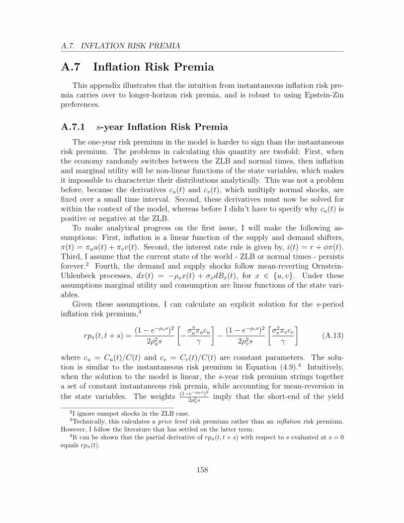
A.7. INFLATION RISK PREMIA
A.7 Inflation Risk Premia
This appendix illustrates that the intuition from instantaneous inflation risk pre-mia carries over to longer-horizon risk premia, and is robust to using Epstein-Zinpreferences.
A.7.1 s-year Inflation Risk Premia
The one-year risk premium in the model is harder to sign than the instantaneousrisk premium. The problems in calculating this quantity are twofold: First, whenthe economy randomly switches between the ZLB and normal times, then inflationand marginal utility will be non-linear functions of the state variables, which makesit impossible to characterize their distributions analytically. This was not a problembefore, because the derivatives cu(t) and cv(t), which multiply normal shocks, arefixed over a small time interval. Second, these derivatives must now be solved forwithin the context of the model, whereas before I didn’t have to specify why cu(t) ispositive or negative at the ZLB.
To make analytical progress on the first issue, I will make the following as-sumptions: First, inflation is a linear function of the supply and demand shifters,π(t) = πuu(t) + πvv(t). Second, the interest rate rule is given by, i(t) = r + φπ(t).Third, I assume that the current state of the world - ZLB or normal times - persistsforever.2 Fourth, the demand and supply shocks follow mean-reverting Ornstein-Uhlenbeck processes, dx(t) = −ρxx(t) + σxdBx(t), for x ∈ u, v. Under theseassumptions marginal utility and consumption are linear functions of the state vari-ables.
Given these assumptions, I can calculate an explicit solution for the s-periodinflation risk premium,3
rpπ(t, t+ s) =(1− e−ρus)2
2ρ2us
[−σ
2uπucuγ
]− (1− e−ρvs)2
2ρ2vs
[σ2vπvcvγ
](A.13)
where cu = Cu(t)/C(t) and cv = Cv(t)/C(t) are constant parameters. The solu-tion is similar to the instantaneous risk premium in Equation (4.9).4 Intuitively,when the solution to the model is linear, the s-year risk premium strings togethera set of constant instantaneous risk premia, while accounting for mean-reversion in
the state variables. The weights (1−e−ρus)22ρ2us
imply that the short-end of the yield
2I ignore sunspot shocks in the ZLB case.3Technically, this calculates a price level risk premium rather than an inflation risk premium.
However, I follow the literature that has settled on the latter term.4It can be shown that the partial derivative of rpπ(t, t+ s) with respect to s evaluated at s = 0
equals rpπ(t).
158

A.7. INFLATION RISK PREMIA
curve loads relatively more on transient shocks than the long-end as shown in Ap-pendix Figure A.15. For example, at a maturity of 4.75 years, corresponding to a5-year inflation swap with three month indexation lag, permanent shocks have about10 times the loading than shocks with a half-life of one year. In contrast, at a matu-rity of 0.75 years the relative weight is only 1.5. Thus, on the short-end we are morelikely to pick up ZLB effects rather than spillovers.
Figure A.15: Weight on inflation risk premia for various maturities and values of ρu, themean-reversion of supply shocks, when the state of the economy (ZLB or non-ZLB) persistspermanently.
0 0.1 0.2 0.3 0.4 0.5 0.6 0.70
0.5
1
1.5
2
2.5
Weig
ht o
n I
nfla
tion
Ris
k P
rem
ia (
Pe
rsis
tent
Sta
te)
Mean−Reversion of Supply Shock
Maturity = 0.75 years
Maturity = 1.75 years
Maturity = 2.75 years
Maturity = 4.75 years
When the ZLB persists forever, there are no spillovers into normal times andsupply shocks are contractionary in the baseline model, cu(t) > 0 (Proposition 4).This is problematic, because it will make inflation risk premia unambiguously nega-tive at the ZLB, so that empirical evidence of positive risk premia becomes hard tointerpret. To address this issue, I allow supply shocks dBu(t) to be correlated withdemand shocks dBv(t). If this correlation is negative, then negative supply shocksmay be (on average) contractionary at the ZLB because they coincide with nega-tive demand shocks, and this can rationalize a positive risk premia at the ZLB. Tosimplify the algebra, I assume that the demand and supply shifters are identicallydistributed, σu = σv = σx and ρu = ρv = ρx, and that the correlation between theBrownian Motions is given by ϕ.
159

A.7. INFLATION RISK PREMIA
Given these assumptions, the s-period inflation risk premium is given by,
rpπ(t, t+ s) =(1− e−ρxs)2
2ρ2xs
[−σ
2xπu(cu + ϕcv)
γ− σ2
xπv(cv + ϕcu)
γ
](A.14)
In normal times, the sign of risk premium in Equation (A.14) is ambiguous whenϕ = 0, because negative supply shocks are contractionary and will generate positiverisk premia, whereas demand shocks will generate negative risk premia. Thus, ifcontractionary supply shocks are the most important source of inflation volatility,then the inflation risk premium will be positive.
At the ZLB, negative supply shocks are expansionary in standard models whenthere are no spillovers, so that the risk premium is unambiguously negative if ϕ = 0.However, if the correlation ϕ is negative, then negative supply shocks will be (onaverage) paired with negative demand shocks, which allows negative co-movementbetween inflation and consumption, effectively mimicking the behavior of contrac-tionary negative supply shocks. This will be the case when cu + ϕcv < 0, makingthe first term in brackets positive. If, in addition, supply shocks dominate inflationvolatility, πu πv, then the overall inflation risk premium is positive. Thus, theconclusions are qualitatively similar to the instantaneous case, which is summarizedas follows.5
Summary 6 In the standard CCAPM, s-year inflation risk premia are positive, innormal times or at the ZLB, if and only if negative supply shocks have contractionaryeffects on average, and this constitutes a significant fraction of aggregate inflationrisk.
In addition, inflation risk premia also capture supply shocks that occur after theeconomy has exited from the ZLB, which raises the observed inflation risk premium.Since the probability of exit over a one-year horizon is relatively small, these ef-fects are less likely to show up at short maturities. This intuition is confirmed inAppendix Figure A.16. In this exercise, I let a standard linearized new Keynesianmodel start at the ZLB and revert permanently to normal times with probability λdtover an interval dt. In addition, I abstract from demand shocks and only considersupply shocks. While the solutions for consumption and inflation can be analyticallycharacterized as in Appendix A.1, this is not true for the inflation risk premium.Thus, these results are calculated by numerically integrating over the stochasticZLB duration. I set λ = 0.5 implying an expected duration of the ZLB of two years.
5Another possibility to rationalize positive inflation risk premia at the ZLB is to make positivedemand shocks deflationary so that cv(πv + ϕπu) < 0. In fact, if inflation risk premia are positiveand cu+ϕcv < 0, then it must also be the case that cv(πv +ϕπu) < 0, because ϕ < 0 and πu πv.This is the consequence of assuming a statistical correlation between demand and supply shocks: ifnegative supply shocks are paired with negative demand shocks, then positive demand shocks mustbe paired with positive supply shocks.
160

A.7. INFLATION RISK PREMIA
In Appendix Figure A.16, the inflation risk premia exhibit hump-shapes at allmaturities. These occur as the inflation risk premium is zero at ρu = 0 becausethe long-run Phillips curve is vertical and zero at ρu → ∞ because such temporaryshocks to not affect consumption or inflation. At a nine-month horizon inflation riskpremia are predominantly negative as most negative supply shocks over this intervalwill be expansionary – the only exception being close-to-permanent shocks for whichthe “Paradox of Toil” does not apply. In contrast, at longer maturities risk premiarise and are predominantly positive as the probability of exit is (cumulatively) higher.Note also that this figure now includes jump risk from the ZLB into normal times.
Figure A.16: Inflation risk premia for various maturities and values of ρu (the mean-reversion of supply shocks) when there is stochastic exit from the ZLB.
0 0.1 0.2 0.3 0.4 0.5 0.6 0.7−3
−2
−1
0
1
2
3
4x 10
−3
Inflatio
n R
isk P
rem
ia
Mean−Reversion of Supply Shock
Maturity = 0.75 years
Maturity = 1.75 years
Maturity = 2.75 years
Maturity = 4.75 years
The calibration is as in Table 4.2, except that φy = 0, ν = 0, % = 0, and σu = 0.1.
Summary 7 In the standard CCAPM, s-year inflation risk premia at the ZLB aremore likely to be negative the smaller s. This is because over a shorter interval exitfrom the ZLB becomes less likely.
A.7.2 Epstein-Zin Inflation Risk Premia
Piazzesi and Schneider (2006) show that Epstein-Zin utility is a key ingredient
161

A.7. INFLATION RISK PREMIA
for rationalizing an upward sloping yield curve given the historical correlations ofconsumption and inflation. Thus, in this subsection I show that my results arerobust to this particular preference specification.
I use the simplifying assumption from the beginning of the previous section andconsider a consumer with Epstein-Zin utility with IES equal to 1 and risk aversionγ−1. Then the continuous time limit of the recursive definition of the value functionimplies,
Etd lnV (t) = −% lnC(t) + % lnV (t)− (1− %)(1− γ−1)
2σ2v , (A.15)
where σ2v is the variance of lnV (t), which is constant in this linear set-up as the
current state of the economy persists forever. Solving forward and substitutinglnC(t) = cuu(t) + cvv(t) yields,
d lnV (t)− Etd lnV (t) =%
%+ ρucuσudBu(t) +
%
%+ ρvcvσvdBv(t). (A.16)
The continuous time limit of the SDF is in turn given by,
d ln Λ(t)− Etd ln Λ(t) =− [d lnC(t)− Etd lnC(t)]
+ (1− γ−1)[d lnV (t)− Etd lnV (t)],(A.17)
where the second term captures the utility recursion, i.e. deviations from CRRA.Substituting the solution from the previous equation and for consumption yields,
d ln Λ(t)− Etd ln Λ(t) =− cu[1 +
(γ−1 − 1)%
%+ ρu
]σudBu(t)
− cv[1 +
(γ−1 − 1)%
%+ ρv
]σvdBv(t),
(A.18)
so that the price of inflation risk is given by,
rpt = −cuπu[1 +
(γ−1 − 1)%
%+ ρu
]σ2u − cvπv
[1 +
(γ−1 − 1)%
%+ ρv
]σ2v . (A.19)
This is similar to Equation (4.9) except for the additional term in square bracketsinvolving γ−1. Standard calibration set γ−1 ≥ 6, so that EZ utility amplify riskpremia, but do not change their sign. Intuitively, EZ utility also punishes assets thatlose value when there is bad news about the future. Due to persistence of shocks inmy setting (ρx <∞), bad news today is also bad news for the future, so risk premiaget amplified (relative to the log utility case) when risk aversion exceeds one.
162

A.8. SWAP RATE - INFLATION EXPECTATION MATCHING
A.8 Swap Rate - Inflation Expectation Matching
Appendix Table A.3 illustrates the reference price levels, inflation lags, and in-flation expectations sources for inflation swap rates. I match inflation expectationsto risk premia as follows: For the Eurozone the ECB releases quarterly 12 monthahead consensus inflation expectations exactly when the previous month’s inflationdata is released. For example, in January the forecast horizon is from December toDecember. The appropriate match for the inflation swap is the October to Octoberexpected inflation rate. I therefore add (known) CPI inflation of the previous twomonths to the forecast, while proportionally downweighting the original 12 monthforecast. This procedure is appropriate, if the last two months of the 12 month in-flation forecast have a similar inflation rate than the first 10 months. For the U.K.and the U.S. I use the estimates obtained from the Kalman filter procedure in theprevious section. For the U.K., I match the December, January, and February swaprates to the Q4-Q4 forecast, which is appropriate given the two month lag, and av-erage over these months to account for seasonal effects. For the U.S. the matchedforecast is calculated as the weighted average of the 4-quarter forecasts originating2 and 3 months back.
Table A.3: Swap Rate - Inflation Expectations Matching
Country Reference Price Inflation Lag Inflation Expectations Source
U.S. CPI 2-3 Months Kalman filter (Blue-Chip)
U.K. RPI 2 Months Kalman filter (HM Treasury)
Eurozone CPI 3 Months ECB
A.9 Supply Shocks and Credit Frictions
This section shows (a) that oil supply shocks tighten credit availability and raiseborrowing rates, and (b) that technology shocks raise asset spreads in a manner thatis quantitatively consistent with the model in Section 4.5.
A.9.1 Oil Supply Shocks
First, I determine the effect of oil supply shocks on credit standards for firms andhouseholds in Japan. I regress credit standards yt (reported at quarterly frequency
163

A.9. SUPPLY SHOCKS AND CREDIT FRICTIONS
in the Japanese loan officer survey) on four of its own lags, on oil shocks, and onrecession/recovery dummies,
yt = α +4∑j=1
βjyt−j +4∑j=0
γjoilt−j + I(recessiont == 1) + I(recoveryt == 1) + εt,
164

A.9.
SUPPLY
SHOCKSAND
CREDIT
FRIC
TIO
NS
Figure A.17: Impact of oil shocks on credit standards in Japan.
0 1 2 3 4 5 6 7 8 9 10 11
−8
−6
−4
−2
0
2
Quarter
Sm
all F
irm
s
(a) Credit Standards: Small Firms.
0 1 2 3 4 5 6 7 8 9 10 11
−9
−8
−7
−6
−5
−4
−3
−2
−1
0
1
Quarter
Me
diu
m F
irm
s
(b) Credit Standards: Medium Firms.
0 1 2 3 4 5 6 7 8 9 10 11
−6
−5
−4
−3
−2
−1
0
1
2
Quarter
Larg
e F
irm
s
(c) Credit Standards: Large Firms.
0 1 2 3 4 5 6 7 8 9 10 11
−6
−5
−4
−3
−2
−1
0
1
2
Quarter
House
hold
s
(d) Credit Standards: Households.
Negative IRFs indicate a tightening of credit standards. 95% confidence intervals are derived by Monte-Carlo draws from anormal distribution with variance equal to the estimated Driscoll-Kraay covariance matrix. Units are calculated as (percentageof respondents selecting “eased considerably” + percentage of respondents selecting “eased somewhat” * 0.5 ) -( percentageof respondents selecting “tightened considerably” + percentage of respondents selecting “tightened somewhat” * 0.5).
165

A.9. SUPPLY SHOCKS AND CREDIT FRICTIONS
Note that I conduct the regression in levels because the data is already reportedas changes in credit conditions.
I plot the resulting impulse response functions in Appendix Figure A.17. Thetightening of credit availability persists for about two years for both firms and house-holds, and (consistent with this interpretation) credit tightens more for small firmsthan for medium firms, which in turn are more affected than large firms. Theseresults indicate that a decline in credit supply is contributing to the contractionfollowing negative supply shocks.
Second, I investigate the effect of oil shocks at the intensive margin. Columnone of Appendix Table A.4 replicates the estimate from Figure 4.3 for the 10-yearbond rate in Japan. Column two conducts the same regression but with the loanspread as a dependent variable. This spread is calculated as the differences betweenlong-term borrowing rates at Japanese commercial banks and the 10-year bond rate.The results show the decline in bond yields is more than fully offset by the rise in theborrowing spread, i.e. private borrowing becomes more expensive after an oil supplyshock. Thus, an Euler equation consumer, who faces these interest rates, wouldcontract her consumption given the rise in borrowing rates. This suggests that boththe intensive and extensive margin of loan supply contribute to the contractionaryeffects of oil supply shocks.
A.9.2 Technology Shocks
Since the model’s forcing process is the technology shock a(t), I verify the quan-titative properties of the model utilization-adjusted TFP series for the U.S. fromFernald (2009). This is a closer match with a(t) in the model than using oil supplyshocks. The Fernald-series is only available for the U.S., and unfortunately similarseries are not available for the other countries in my sample.
I determine the effect of technology shocks on the three-month TED spread, i.e.the spread between the three-month interbank borrowing rate and the three-monthTreasury-Bill. While the baseline model in Section 4.5 does not contain an interbankmarket, it can be easily extended along this dimension following Gertler and Kiyotaki(2010). In such an extension, the TED spread corresponds to the spread ω(t) in themodel – i(t) is the government bond yield and loans to other banks are subject tothe incentive constraint and must earn i(t) +ω(t). Thus, by using the Fernald-seriesand the TED spread I stay as close to the model as possible.
In Appendix Figure A.19(a) I report the effect of a 1% negative TFP shock on theTED spread, estimated from an ADL equation with 12 lags. The TFP shock raisesthe TED spread by up to 24 basis points after eight quarters. I compute the corre-sponding model statistic by linearizing the model around the non-stochastic steadystate, setting ρa = 0 as in the Fernald-series. The IRF is plotted in Appendix Fig-ure A.19(b), and shows that a 1% permanent TFP shock raises the borrowing-lending
166

A.9. SUPPLY SHOCKS AND CREDIT FRICTIONS
Table A.4: Response of Japanese Bond Rate and Loan Spread to Oil Supply Shock
Change in Bond RateChange in Loan Spread
(Loan Rate - Bond Rate)
Oil Shock -0.0416** 0.0588**
(0.0207) (0.0233)
Dep. Var. Lags 36 36
Observations 154 154
Driscoll-Kraay standard errors in parentheses
∗ p < 0.1, ∗∗ p < 0.05, ∗∗∗ p < 0.01
167

A.10. OIL SHOCKS IN INCOMPLETE MARKETS
spread by 25 basis points on impact, which subsequently declines to zero. This sug-gests that the credit frictions in this calibration are empirically reasonable.
A.10 Oil Shocks in Incomplete Markets
This appendix shows how oil shocks propagate in an open economy with incom-plete markets. The set-up builds on Farhi and Werning (2012a) and Wieland (2012).There are two countries home (H) and the rest of the world (F). The home economyis small and must import oil from the rest of the world.
A.10.1 Set-up
Home agents maximize the stream of utility,∫ ∞0
e−ρt[C(t)1−σ
1− σ− χN(t)1+ν
1 + ν
],
where C(t) is domestic consumption and N(t) is labor. The inverse of the intertem-poral elasticity of substitution is σ, the inverse of the Frisch elasticity is ν, and χ isa parameter that determines steady-state labor supply.
Consumption is an aggregate of domestically produced goods CH(t) and foreignproduced goods CF (t)
C(t) =[(1− α)
1ηCH(t)
η−1η + α
1ηCF (t)
η−1η
] ηη−1
,
which are themselves aggregates of individual varieties,
Cx(t) =
(∫ 1
0
Cx(t, j)ε−1ε dj
) εε−1
, x ∈ H,F.
The price of home consumption in home currency is given by
P (t) =[(1− α)PH(t)1−η + αPF (t)1−η] 1
1−η .
Home asset holdings of the risk-free bond D(t) evolve according to
D(t) = i(t)D(t)− P (t)C(t) +W (t)N(t) + Π(t),
where i(t) is the nominal interest rate, W (t) the wage rate, and Π(t) are profits fromfirms.
Firms produce output Y (t, j) of variety j according to a CES technology,
Y (t, j) =[(1− γ)
1ψN(t, j)
ψ−1ψ + γ
1ψX(t, j)
ψ−1ψ
] ψψ−1
168

A.10. OIL SHOCKS IN INCOMPLETE MARKETS
Figure A.18: TFP Shocks and Credit Spreads
0 2 4 6 8 10 12 14 16 18
−0.1
0
0.1
0.2
0.3
0.4
0.5
0.6
Quarters
LIB
3−
TB
3 S
pre
ad (
% p
oin
ts)
(a) TED Spread.
0 0.5 1 1.5 2 2.5 3 3.5 4 4.5 50
0.5
1
1.5
2
2.5
3x 10
−3
Bo
rrow
ing
−Le
nd
ing S
pre
ad
Years
(b) Model Borrowing Spread.
Left Panel: Impact of 1% permanent, negative TFP Shock on TED Spread (3 monthLIBOR - 3 month Treasury Bill). Estimated using an ADL equation with 12 lags of theTED spread and 12 lags of TFP shock. Newey-West standard error bands are drawn fromthe Variance-Covariance matrix using Monte-Carlo methods. Right Panel: Model impactof a 1% permanent, negative TFP shock on the borrowing-lending spread given the baselinecalibration with ρa = 0.
169

A.10. OIL SHOCKS IN INCOMPLETE MARKETS
where X(t, j) is oil input, γ the steady-state share of oil in production, and ψ itselasticity of substitution with labor input. Firms face standard Calvo pricing frictionswhere prices can be reset with probability (ρδdt over an interval dt.
The foreign economy is large relative to the domestic economy. Thus, the shareof home goods in foreign consumption is close to zero α∗ → 0. Otherwise the foreigneconomy is set-up as the home economy. I denote foreign quantities with a ∗, i.e.C∗(t) is foreign consumption. In addition the foreign economy is endowed with astochastic supply of oil X(t), that evolves according to
d ln X(t) = −ρx ln X(t) + σxdBx(t).
The shock dBx(t) is the only disturbance in the model. The initial condition isln X(0) = 0. I consider a situation where dBx(0) < 0, i.e. a negative oil supply shock,and dBx(t) = 0 for all t > 0. Thus, as in Farhi and Werning (2012a), I compute aperfect foresight equilibrium. This makes the computation of the incomplete marketmodel more convenient as the Pareto weight (defined below) only changes once invalue.
I define the following relative prices. The real exchange rate Q(t) is equal to
Q(t) =E(t)P ∗(t)
P (t),
where E(t) is the nominal exchange rate. The terms of trade equal
S(t) =PF (t)
PH(t),
and the relative price of oil equals
O(t) =PX(t)
PH(t).
I assume that the law of one price holds.The central bank follows a standard interest rate rule subject to the zero bound
constraint.i(t) = maxρ+ φπ(t), 0.
A.10.2 Equilibrium
In equilibrium the following first order conditions must be satisfied. Both homeand foreign satisfy an Euler equation,
σdC(t)
C(t)= (i(t)− π(t)− ρ)dt.
170

A.10. OIL SHOCKS IN INCOMPLETE MARKETS
Labor is supplied allocated according to
χC(t)σN(t)ν =W (t)
P (t)
where the RHS equals the real wage. Domestic and foreign consumption are relatedby
C(t) = ΘC∗(t)Q(t)1σ ,
where Θ is the relative Pareto weight. Relative demands for varieties are given bythe standard Dixit-Stiglitz relationships.
The first order condition for the firms reset price P r(t) is given by,∫ ∞0
e−ρδs−∫ s0 i(t+s)
[(1− ε) + ε(1− τL)
W (t+ s)/P (t+ s)
MPL(t+ s)P r(t)
]Y (t+ s, i)ds = 0,
where MPL(t+ s) is the marginal product of labor and τL is a labor input subsidy.In addition an equilibrium must satisfy the feasibility conditions. Domestic and
foreign output must be equal to domestic and foreign consumption respectively
Y (t) = CH(t) + C∗H(t), Y ∗(t) = CF (t) + C∗F (t) = C∗(t),
where the last two equality follows from the fact that the foreign economy is large.In addition the quantity of oil supplied must equal the quantity of oil demanded,
X(t) = XF (t) +XH(t) = XF (t).
Finally, net foreign assets (denominated in home currency) evolve according to
dNFA(t) = (PH(t)C∗H(t)− PF (t)CF (t)− PX(t)XH(t)) + i(t)NFA(t),
so the home country accumulates assets through exports and draws down assets byimporting either consumption goods or oil.
The equilibrium under complete markets features Θ = 1, whereas in the equilib-rium under incomplete markets NFA(0) is given.
A.10.3 Computation
To solve for the equilibrium I log-linearize the equilibrium conditions. Small capsletters denote these log-linearized quantities. I then proceed in two steps. First,I solve for the allocation in the foreign economy. Since this economy is large itsallocation is independent of the behavior of the home economy. Next, taking theallocation for the foreign economy as given, I compute the allocation for the homeeconomy.
171

A.10. OIL SHOCKS IN INCOMPLETE MARKETS
A.10.4 Foreign Economy
The solution to the foreign economy under complete and incomplete markets isidentical. When the ZLB does not bind, then it is given by,
y∗(t) = c∗(t) =σ−1(φ− 1)γµ
σ−1λ(φ− 1) + (1− γ)ρx(ρ+ ρx)x(t),
π∗(t) =−ρxγµ
σ−1λ(φ− 1) + (1− γ)ρx(ρ+ ρx)x(t),
n∗(t) = −γκ(φ− 1)(σψ)−1(σψ − 1) + γρx(ρ+ ρx)
σ−1λ(φ− 1) + (1− γ)ρx(ρ+ ρx)x(t),
where the parameters µ and λ are defined as
µ =κ
ψ(1 + νψ), λ = µ+
κ
ψ(1− γ)(σψ − 1),
and κ is the slope of the new Keynesian Phillips curve. Note that a negative supplyshock lowers consumption and output, but may raise GDP (here equal to labor input)depending on parameters.
The price of oil abroad is equal to,
o∗(t) = − 1
ψ
(φ− 1)σ−1κ(ν + σ)(1− γ) + ρx(ρ+ ρx)(1 + γνψ)
σ−1λ(φ− 1) + (1− γ)ρx(ρ+ ρx)x(t).
It is immediate that negative oil supply shocks lower consumption, raise inflation,and raise real oil prices.
To illustrate the effects of the ZLB, I follow Farhi and Werning (2012a) andconsider the case where the central bank interest rate is exogenous with respect tothe oil shock (e.g., fixed at zero). In this case, the allocation for the foreign economyis given by,
c∗,ZLB(t) = − σ−1γµ
−σ−1λ+ (1− γ)ρx(ρ+ ρx)x(t),
π∗,ZLB(t) =−ρxγµ
−σ−1λ+ (1− γ)ρx(ρ+ ρx)x(t),
n∗,ZLB(t) =γκ(σψ)−1(σψ − 1)− γρx(ρ+ ρx)
−σ−1λ+ (1− γ)ρx(ρ+ ρx)x(t),
Note that (1 − γ)ρx(ρ + ρx) > σ−1λ is a necessary condition for a unique boundedequilibrium to exist (see also Appendix A.1). The same condition also guaranteesthat real GDP and real oil prices rise following a negative supply shock,
o∗,ZLB(t) = − 1
ψ
−σ−1κ(ν + σ)(1− γ) + ρx(ρ+ ρx)(1 + γνψ)
−σ−1λ+ (1− γ)ρx(ρ+ ρx)x(t).
Thus negative oil supply shocks raise consumption at the ZLB, raise real GDP (laborinput), raise inflation, and raise real oil prices.
172

A.10. OIL SHOCKS IN INCOMPLETE MARKETS
A.10.5 Home Economy
In a complete market setting, home and foreign are affected symmetrically by theoil shock. Thus the allocation for the home country are the same as abroad, both innormal times,
cCM(t) = c∗(t), πCM(t) = π∗(t),
oCM(t) = o∗(t), nCM(t) = n∗(t),
and at the ZLB,
cZLB,CM(t) = c∗,ZLB(t), πZLB,CM(t) = π∗,ZLB(t),
oZLB,CM(t) = o∗,ZLB(t), nZLB,CM(t) = n∗,ZLB(t).
Note in particular, that these solutions are independent of the import share α.When markets are incomplete I consider the case where α → 0 and ν = 0. This
significantly simplifies the computation of the new Pareto weight θ = log Θ. Asin Farhi and Werning (2012a) the incomplete market allocation is the sum of twocomponents – the complete market allocation and an additional term,
cIM(t) = cCM(t) + δIMc , πIM(t) = πCM(t) + δIMπ ,
oIM(t) = oCM(t) + δIMo , nIM(t) = nCM(t) + δIMn
These additional δIM -terms are independent of time because the home economy isforward looking and thus instantaneously adjusts according to the new wealth level.
With zero initial net financial assets, NFA(0) = 0, I use the evolution of the netfinancial asset position to solve for the new Pareto weight θ. Since the no-ZLB andZLB region generate different consumption paths, the Pareto weight will also varyaccordingly,
θ =ρ
(ρ+ ρx)
σγρx(ρ+ ρx)/(1− γ) + (φ− 1)µ(1− ψ)
[λ(φ− 1) + σ(1− γ)ρx(ρ+ ρx)][1 + σ(ψ − 1) + (1− γ)(ση − 1)]dB(0),
and,
θZLB =ρ
(ρ+ ρx)
σγρx(ρ+ ρx)/(1− γ)− µ(1− ψ)
[−λ+ σ(1− γ)ρx(ρ+ ρx)][1 + σ(ψ − 1) + (1− γ)(ση − 1)]dB(0).
Note that the Pareto weights may be of different signs if the oil share in productionγ is sufficiently small. For instance, suppose that ψ < 1 so labor and oil are not verysubstitutable. In normal times a decline in oil supply raises oil prices, which increasesimport costs for domestic suppliers. In addition, the decline in foreign demand forhome goods further deteriorates the home net foreign asset position. Thus, in normaltimes θ < 0 as the foreign country accumulates net assets relative to the domestic
173

A.10. OIL SHOCKS IN INCOMPLETE MARKETS
economy. At the ZLB, however, foreign consumption increases after a negative oilsupply shock, which raises foreign demand for home goods. The increase in exports islarger than the increase in input costs if γ is small, so the home country accumulatesnet foreign assets and θ > 0. Thus, at the ZLB, a decline in foreign oil productiondoes not necessarily transfer resources from the home country to the foreign country.
Given θ, we can calculate the incomplete market component of the home alloca-tion as follows
δIMc = γθ, δIMπ = 0, δIMo = −(1− γ)σθ, δIMn = −γ[(1− γ)(ση − 1) + σψ]θ. (A.20)
We can now assess whether incomplete markets are sufficient to explain the estimatedIRFs in Section 4.3.1. First, temporary negative supply shocks are expansionary inthe complete market solution at the ZLB, cZLB,CM(t) > 0 and nZLB,CM(t) > 0.Since these expansionary effects are temporary, we have cZLB,IM(t) > δZLB,IMc =cZLB,IM(∞) and nZLB,IM(t) > δZLB,IMn = nZLB,IM(∞). Thus, in the short-run anegative oil supply shock at the ZLB should be more expansionary than in the long-run. However, in Figure 4.2 we see the opposite pattern — negative supply shocksare more contractionary in the short-run. Intuitively, in the short-run the economybenefits from higher inflation and lower real interest rates, irrespective of the wealthtransfers that matter for the long-run equilibrium. This very general result suggeststhat incomplete markets by themselves are not sufficient to account for the empiricalfindings. One still needs a model where the short-run effect of negative supply shocksis contractionary at the ZLB, such as the model in Section 4.5.
Furthermore, there are other aspects of this allocation that suggest that incom-plete markets are not sufficient to match the data. First, irrespective of whetherthe home country becomes a net debtor or creditor, Equation (A.20) shows thatconsumption and GDP (labor input) move in opposite directions. For example, ifwealth declines then consumption falls but real GDP rises to produce the exportsnecessary to pay down the debt. This contrasts with the empirical results whereboth consumption and labor input fall following a negative supply shock.
Second, in this allocation θ and θZLB have opposite signs. Thus, if the incompletemarket effects are strong we should see that negative supply shocks have qualitativelydifferent effects in normal times than at the ZLB. However, in the data oil shocksare contractionary in both settings and only differ in their quantitative magnitude.
In summary, the results from this section show that incomplete markets by them-selves cannot explain the contractionary effects of oil supply shocks at the ZLB andin normal times. While they may explain part of the contractionary effect, the creditfriction is still necessary to match the data. Of course, it is possible that the creditfriction and the incomplete market effects reinforce each other, thereby contributingto the contractionary effects of oil supply shocks at the ZLB. I leave the investigationof such interaction effects for further research.
174

A.11. MODEL SOLUTIONS
A.11 Model Solutions
This appendix examines the computational properties of the model. In the firstsubsection, I examine how closely Equation (4.13) captures the solution in the lin-earized model with three state variables. In the second subsection, I lay out thecomputational strategy for the non-linear model with one state variable and com-pute Euler equation residuals.
A.11.1 Accuracy of State Space Reduction
This section examines how closely equation (4.13) captures the solution to thethree state variable model in Section 4.5. First, the model equation of the three-state-variable model and the one-state-variable model are linearized and solved usingthe Matlab code described in Sims (2002). This code is available for download onChris Sims’ website. Appendix Figure A.19 displays the resulting impulse responsefunctions of the standard New Keynesian model, the three state variable model,and the one state variable friction model to a 1% TFP shocks. Overall, the modelsdisplay very similar behavior in the responses of output, consumption, inflation, andthe banking variables. While the dynamics of the interest rate spread are somewhatdifferent in the two models, what matters for a borrower’s consumption choice is theintegral over the spread IRF. The integrals are very similar across the two modelsso there is little difference in consumption behavior of borrowers. Thus the one-state-variable model delivers essentially the same results, but greatly simplifies thenon-linear computation.
Second, I solve the three-state-variable model using projection methods as out-lined in the following section. Since the state space is significantly larger in thismodel I use polynomials up to degree 5 for each state variable, for a total of 53 = 125polynomials. While this grid is coarse, it can provide insight if the one-state-variablemodel also provides a good approximation to the three-state-variable model at theZLB. In addition, in order to solve this model I have to raise the discount rate slightlyto % = 0.01275 (compared to % = 0.0125 in the baseline) and lower the volatility toσa = 0.0001 (compared to σa = 0.005 in the baseline). In Appendix Figure A.20 Iplot IRFs from a 1% positive technology shock without the ZLB. As in the linearizedcase, the IRFs of the one-state-variable model and the three-state-variable model arevery close. Appendix Figure A.21 shows that equation (4.13) also provides a verygood approximation at the ZLB. In particular, output expands by similar magnitudesin the one-state-variable model and the three-state-variable model.
175

A.11. MODEL SOLUTIONS
A.11.2 Accuracy of Non-linear Solution
The model is computed by iterating over the FOCs, while using Chebychev poly-nomials to approximate equilibrium objects. I use polynomials up to degree 33 inthe computation. The initial guess is the (linear) solution to the standard NewKeynesian model. Convergence is fast, taking about 20 seconds using the baselinecalibration.
The residuals from the two Euler equations (lender and borrower) as well as fromthe Phillips Curve are plotted in Appendix Figure A.22. The errors in the PhillipsCurve are of trivial magnitude (10−14) and can be ignored. Similarly, the Eulerequation errors ignoring the ZLB are very small (10−13). The ZLB introduce largererrors because the approximation will not perfectly capture when the ZLB starts tobind. Thus, the errors are largest at the border of the ZLB and non-ZLB regions.However, the maximum errors are still small: at most 3.5 basis points in the standardmodel and 1.2 basis points in the friction model.
176

A.11.
MODELSOLUTIO
NS
Figure A.19: IRFs of Standard NK model, Friction Model with Three State Variables, and Friction Model with OneState Variable to a 1% TFP shock.
0 2 4−15
−10
−5
0
5x 10
−3Supply Shock
0 2 40
2
4
6x 10
−3Consumption: Lender
0 2 40
0.005
0.01Consumption: Borrower
0 2 40
2
4
6
8x 10
−3 Output
0 2 4−2
−1.5
−1
−0.5
0x 10
−3 Inflation
0 2 4−6
−4
−2
0x 10
−3Interest Rate
0 2 4−2
0
2
4
6x 10
−3 Borrowing
0 2 40
0.005
0.01
0.015
0.02Asset Prices
0 2 4−0.01
−0.005
0MV of Net Worth
0 2 40
0.005
0.01
0.015
0.02Net Worth
0 2 4−4
−3
−2
−1
0x 10
−3 Spread
Standard NK
Friction Model
Friction w/ Approximation
IRFs are calculated from linearized solution to each model.
177

A.11.
MODELSOLUTIO
NS
Figure A.20: IRFs of Friction Model with Three State Variables and Friction Model with One State Variable to a1% TFP shock assuming that ZLB does not bind.
0 1 2 3 4 50
0.002
0.004
0.006
0.008
0.01Technology Shock
0 1 2 3 4 50
2
4
6
8x 10
−3 Output
0 1 2 3 4 5−1.5
−1
−0.5
0x 10
−3 Inflation
0 1 2 3 4 5−4
−3
−2
−1
0x 10
−3 Interest Rates
0 1 2 3 4 5−4
−3
−2
−1
0x 10
−3 Spread
Friction Model
Friction Model w/ Approx.
IRFs are calculated from non-linear model using projection methods.
178

A.11.
MODELSOLUTIO
NS
Figure A.21: IRFs of Friction Model with Three State Variables and Friction Model with One State Variable to a1% TFP shock when the ZLB binds.
0 1 2 3 4 50
0.002
0.004
0.006
0.008
0.01Technology Shock
0 1 2 3 4 50
1
2
3
4
5
6x 10
−3 Output
0 1 2 3 4 5−1.5
−1
−0.5
0x 10
−3 Inflation
0 1 2 3 4 5−20
−15
−10
−5
0
5x 10
−4 Interest Rates
0 1 2 3 4 5−4
−3
−2
−1
0x 10
−3 Spread
Friction Model
Friction Model w/ Approx.
IRFs are calculated from non-linear model using projection methods.
179

A.11.
MODELSOLUTIO
NS
Figure A.22: Residuals of dynamic equations in non-linear solution.
−0.05 −0.04 −0.03 −0.02 −0.01 0 0.01 0.02 0.03 0.04 0.05−3
−2
−1
0
1
2
3
4
5x 10
−4
Eu
ler
Eq
ua
tion
Resid
uals
: Le
nd
er
Technology Level a(t)
ZLB Binds
Standard Model
Standard Model with ZLB
Friction Model
Friction Model with ZLB
(a) Euler Equation: Lender
−0.05 −0.04 −0.03 −0.02 −0.01 0 0.01 0.02 0.03 0.04 0.05−3
−2
−1
0
1
2
3
4
5x 10
−4
Eule
r E
quation R
esid
uals
: B
orr
ow
er
Technology Level a(t)
ZLB Binds
Standard Model
Standard Model with ZLB
Friction Model
Friction Model with ZLB
(b) Euler Equation: Borrower
−0.05 −0.04 −0.03 −0.02 −0.01 0 0.01 0.02 0.03 0.04 0.05−4
−3
−2
−1
0
1
2x 10
−14
Phill
ips C
urv
e R
esid
uals
Technology Level a(t)
ZLB Binds
Standard Model
Standard Model with ZLB
Friction Model
Friction Model with ZLB
(c) Phillips Curve
180

Appendix B
Appendix to Chapter 3
B.1 Complete Model
B.1.1 Households
Each country is populated by a representative household. The objective functionfor the household in the home country is given by,
maxCt,Nt∞t=0
E0
∞∑t=0
(t∏
s=0
βs
)[C1−σt
1− σ− χt
N1+νt
1 + ν
], (B.1)
where Ct is domestic consumption and Nt is domestic labour supply. The discountfactor βt follows a stationary stochastic process with steady state value β. At time t,the household knows next period’s value of the stochastic discount factor, βt+1, as wellas its history, but it does not know any other future values with certainty. Discountfactor shocks are a standard method to generate a liquidity trap (see Christiano,Eichenbaum, and Rebelo (2011) and Eggertsson and Woodford (2003)). σ is theinverse of the elasticity of substitution and ν is the inverse of the Frisch elasticityof labour supply. Finally, χt > 0 governs the steady state labour supply and alsofollows a stationary stochastic process. For the foreign country, I let χ∗ = n−(σ+ν)χ,to make it produce n times as much output than the home country. The homecountry becomes a small open economy as I take the limit n→∞.
The domestic household maximizes its objective (B.1), subject to its budget con-straint each period,
PtCt + Et[Qt,t+1Dt+1] ≤ Dt +WtNt + Tt ∀ t = 0, 1, ... (B.2)
where Pt is the price of the domestic consumption good, Wt is the wage rate fordomestic labor and Tt are net transfers from the government and firms. Dt+1 is avector of payoffs from the portfolio held from time t until t+1. I assume that financial
181

B.1. COMPLETE MODEL
markets are complete, which implies that the stochastic discount factor Qt,t+1 is theunique asset pricing kernel for the vector of payoffs Dt+1.
The optimality conditions for the domestic households are as follows. (For theforeign household there exists an analogous set of first order conditions.) First, themarginal utility of consumption multiplied by the real wage rate must equal themarginal disutility of labor,
C−σtWt
Pt= χtN
νt . (B.3)
Second, the household satisfies the Euler equation,
βtRt+1Et
[(Ct+1
Ct
)−σ (PtPt+1
)]= 1, (B.4)
where Rt+1 is the gross nominal interest rate on the domestic one-period risklessbond.
The asset pricing equations for the home and foreign safe bonds imply that theexcess return of domestic over foreign bonds has a price of zero,
Et
[Qt,t+1
(Rt+1 −
Et+1
EtR∗t+1
)]= 0. (B.5)
Here R∗t+1 is the gross nominal interest rate on the foreign bond and Et is the nominalexchange rate between the home and the foreign currency. The latter is defined asthe quantity of domestic currency for each unit of foreign currency, so that a fallin Et corresponds to an appreciation of the domestic currency. Equation B.5 willbecome an uncovered interest rate parity (UIP) condition in the log-linearized smallopen economy.
The household in the foreign country also satisfied an Euler equation,
βtR∗t+1Et
[(C∗t+1
C∗t
)−σ (P ∗tP ∗t+1
)]= 1, (B.6)
where C∗t is foreign consumption, and P ∗t the foreign price level. Foreign consumptionC∗t is exogenous with respect to the domestic economy, due to the large size of theforeign country.
B.1.2 Final Goods Firms
The production structure in the economy is as follows. In each country there is acontinuum of firms that produce intermediate goods with local labor inputs. Theseintermediate goods are then assembled by final goods firms into the final consumptiongood.
182

B.1. COMPLETE MODEL
For both countries, there are two types of perfectly competitive firms. In the homecountry, one set of firms produces an aggregate CH
t by combining a continuum of
home-produced varieties CHt (j), CH
t =(∫ 1
0CHt (j)
ε−1ε dj
) εε−1
, where ε is the elasticity
of substitution between different domestically-produced varieties. The firms’ costminimization problem implies that home-produced varieties are demanded accordingto the standard Dixit-Stiglitz demands,
CHt (j) =
(PHt (j)
PHt
)−εCHt ,
where PHt (j) is the price of a given variety and PH
t =(∫ 1
0PHt (j)1−εdj
) 11−ε
is the
price of the aggregate CHt . Analogous equations apply to the set of firms in the
foreign country that produce CFt .
The remaining domestic final good firms then combine the aggregates CHt and
CFt into the desired consumption good. In particular, for the home country,
Ct =[(1− γ)
1η (CH
t )η−1η + γ
1η (CF
t )η−1η
] ηη−1
,
where γ is the share of imports in aggregate home consumption and η the elasticityof substitution between home and foreign goods. I define the degree of openness ofan economy to be equal to γ. Intuitively, when γ = 0 the home country will neverimport any goods and it effectively becomes a closed economy.1 When γ = 1, thenthe economy only consumes foreign goods, so it will have to export all its productionto finance this consumption. Since the gross amount of trade increases in γ, I willtreat this parameter as measuring the degree of “openness:” Economies with highervalues for γ are more “open” because they will trade more goods.
Given this particular final consumption good, the optimal choice between thehome produced composite and the foreign goods satisfy the standard Dixit-Stiglitzdemand equations, so that the price of domestic consumption is given by Pt =[(1− γ)(PH
t )1−η + γ(P Ft )1−η] 1
1−η , where P Ft is the domestic price of the foreign con-
sumption aggregate CFt .
To ensure that larger foreign production does not depress the relative price offoreign goods, I assume that the foreign country consumes primarily its own goods.Thus, I let share of imports of domestic output in foreign consumption be decreasingin n, ψ = γ/n. This ensures that the terms of trade in the steady state equal 1.In the small open economy case, where n → ∞, the share of home goods in foreignconsumption approaches zero, ψ → 0.
1In this case the home economy is equivalent to the model in Christiano, Eichenbaum, andRebelo (2011).
183

B.1. COMPLETE MODEL
B.1.3 Intermediate Goods Firms
In each country there is continuum of local firms, producing a differentiatedproduct using local labor. In the home country, these firms produce the varietiesY Ht (j) according to the production function,
Y Ht (j) = AtNt(j),
where Nt(j) is domestic labour input into the production of good j and At is ag-gregate technology, which I assume to be stationary. Each firm sets its prices ona staggered basis: With probability θ its current price remains fixed at last peri-ods price and with probability 1 − θ it is optimally reset. The profit maximizationproblem of firm i is therefore,
maxPHt (i)
Et
∞∑j=0
θjQt,t+j
[PHt (i)− (1− τ)WH
t+j(i)]Yt+j(i), (B.7)
where τ = ε−1 is an employment subsidy designed to offset the inefficiently lowoutput from monopolistic competition. Qt,t+j is the stochastic discount factor ofdomestic residents.
I assume that labour is perfectly substitutable between sectors, which impliesthat the wage paid in each sector, WH
t (j), must be the same in equilibrium. I define
aggregate domestic output analogously to consumption Y Ht =
(∫ 1
0Y Ht (j)
ε−1ε dj
) εε−1
.
B.1.4 Government
Similar to the Dornbusch model, I assume that the government spends money ondomestically produced goods only. In particular, government spending is the same
composite good as CHt , Gt =
(∫ 1
0Gt(j)
ε−1ε dj
) εε−1
. Furthermore, I assume that the
government chooses among varieties to maximize the aggregator Gt. This assumptiongreatly simplifies the derivation of the New Keynesian Phillips Curve.
Government purchases are financed by lump-sum taxation and Ricardian equiv-alence holds in this economy. Subject to the no-Ponzi scheme condition, the govern-ment must satisfy the budget constraint,
B0 =∞∑t=0
(t∏
s=0
1
Rs
)Gt −
∞∑t=0
(t∏
s=0
1
Rs
)Tt, (B.8)
where Tt are lump-sum taxes and B0 are initial government assets. The steady-stateshare of government spending in output is given by g = G/Y .
184

B.1. COMPLETE MODEL
The central bank conducts monetary policy according to a simple Taylor rule,subject to the zero interest rate floor,
Rt+1 = max
β−1Et
(PHt
PHt−1
)φπ, 1
, (B.9)
where φπ > 1 to satisfy the Taylor principle. Note that the central bank is respondingto the inflation of domestically produced goods (the PPI), not the inflation rate ofconsumption goods (the CPI).
B.1.5 Prices and Market Clearing
The terms of trade are defined as the ratio between import prices (in domesticcurrency) and export prices,
St =P Ft
PHt
. (B.10)
I assume that the the law of one price holds among individual goods. This definesthe nominal exchange rate as ratio of the domestic currency price of good j to theforeign currency price of good j,
Et =PHt (j)
PH∗t (j)
=P Ft
P F∗t
. (B.11)
The Backus-Smith condition (Backus and Smith (1993)) in this model is subjectto a reduced form friction Ft. Thus, consumption at home relative to abroad isproportional to the ratio of the real exchange rate λt and the friction Ft,(
C∗tCt
)−σ= λt/Ft. (B.12)
In equilibrium the market clearing conditions for home goods,
Yt(j) = CHt (j) + CH∗
t (i) +Gt(j) ∀ j, (B.13)
as well as for foreign goods have to be satisfied. The definition of the equilibrium inthis model is then as follows.
Definition 8 (Equilibrium) The equilibrium is a sequence,
CHt (i), CF
t , Nt(i), Yt(i), Dt, Gt(i), Tt,WHt , P
Ht (i), PH∗
t , P Ft , P
∗t , Rt+1, R
∗t+1, St, Et∞t=0,
such that for given C∗t , Gt, βt, χt, At∞t=0 and given initial assets D0, B0 the max-imization problems for the domestic and foreign households and firms are satisfied;
185

B.2. BACKUS-SMITH WITH WEDGE: AN EXAMPLE
the government satisfies its budget constraint (B.8) and allocates spending to maxi-mize Gt; the domestic nominal interest rate follows the Taylor rule (B.9); the foreignreal interest rate is determined by the foreign Euler equation (B.6); the Backus-Smithcondition (B.12) is satisfied; domestic and foreign prices satisfy the law of one price(B.11); and the market clearing conditions for the home and foreign goods are satis-fied.
B.2 Backus-Smith with Wedge: An Example
Following Bodenstein (2008), consider a two country economy with limited en-forcement of international contracts. In particular, they can only be enforced throughthreat of exclusion from asset markets in the future. Let Vt denote the home coun-tries value from financial autarky. Then the incentive compatibility constraint mustsatisfy,
Et
∞∑s=0
βsu(ct+s) ≥ Vt ∀t
Denote the Lagrange multiplier on this constraint by µt. Then the objective functionof the home agent can be rewritten as
E0
∞∑t=0
βt
[u(ct) + µtEt
∞∑s=0
βsu(ct+s)− Vt
]= E0
∞∑t=0
βt [Mtu(ct) + µt (u(ct+s)− Vt)]
where Mt+1 = Mt + µt and M0 = 1. The first order conditions for the domestichousehold are,
λtPt = [Mt + µt]u′(ct)
where Pt is the price of consumption, and
Qt,t+1 = βλt+1
λt
is the home agents SDF. Absent arbitrage opportunities, the home and foreign SDFare equal, which implies (given symmetric initial conditions)
u′(c∗t )
u′(ct)= λt
Mt+1
M∗t+1
where λt is the real exchange rate and M∗t+1 analogously defined for the foreign
country. Log-linearizing this equation yields,
σ(ct − c∗t ) = λt − ft
where ft = mt+1 − m∗t+1, which is the expression (3.1) in the baseline model.
186

B.3. SOLUTION METHOD FOR BASELINE MODEL
B.3 Solution Method for Baseline Model
The zero lower bound on nominal interest rates makes this model piecewise linear.
In particular, let xt =(yt ct πt st rt+1
)′be the vector of endogenous variables
and υt =(gt βt c∗t
)′be the vector of exogenous variables. So long as the liquidity
trap does not bind, we can write the system of equations as
Axt = BEtxt+1 + Fυt. (B.14)
Given the stochastic process in Example 1, its unique solution when the zerolower bound does not bind is
xt = Dυt,
where D = (I − A−1Bdiag(p))−1A−1F . Because there are no endogenous statevariables in this model, a shock in period t causes an immediate jump in xt to thenew equilibrium. If at t + 1 the shock disappears then the economy jumps back tothe steady state. On the other hand, if the shock remains at the same value, thenxt+1 = xt. In particular, the fiscal multiplier outside the liquidity trap is the D11
element in the matrix D scaled by g−1, the inverse of the government’s share inoutput. Because the system of equations is linear, this multiplier is independent ofthe size of government spending.
The liquidity trap is somewhat more difficult to handle. When the economy is atthe zero lower bound at time t, the system of equations may be written as follows,
A∗xt = BEtxt+1 + C∗ + Fυt, (B.15)
where A∗ is the same matrix as A except that the A∗53 entry is equal to zero whereasA53 = −φ. This reflects that in the liquidity trap, the nominal interest rate isbounded at zero and does respond to changes in the inflation rate. Instead, the log-linearized nominal interest rate is equal to −r, which is captured in the C∗51 elementof the vector C∗. All other elements of this vector are zero.
If the law of motion is given by equation (B.15) for all t = 0, 1, ..., then thereis no unique solution to this system of equations because the economy violatesthe Taylor principle. To avoid this case I require that the economy must ulti-mately exit the liquidity trap with probability 1. This will imply that in thelimit, the law of motion must satisfy equation (B.14) (rather than (B.15)), whichwe know has a unique solution. Given the stochastic process I have assumed,limj→∞ Prob [υt+j = 0|υt 6= 0] = 1. We therefore know that, in the limit, any shockthat causes the zero bound to bind will disappear with probability one. Since we exitthe liquidity trap with probability 1, the Taylor principle will hold asymptoticallyand there will be a unique solution to this problem.
187
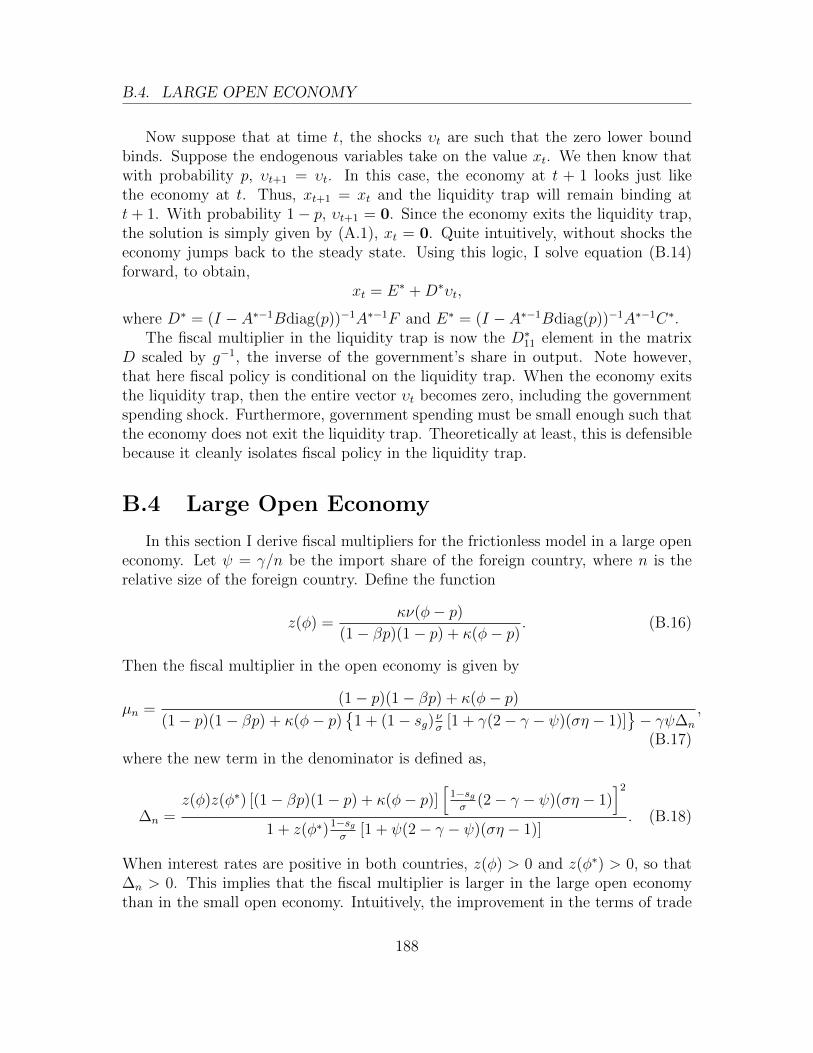
B.4. LARGE OPEN ECONOMY
Now suppose that at time t, the shocks υt are such that the zero lower boundbinds. Suppose the endogenous variables take on the value xt. We then know thatwith probability p, υt+1 = υt. In this case, the economy at t + 1 looks just likethe economy at t. Thus, xt+1 = xt and the liquidity trap will remain binding att + 1. With probability 1− p, υt+1 = 0. Since the economy exits the liquidity trap,the solution is simply given by (A.1), xt = 0. Quite intuitively, without shocks theeconomy jumps back to the steady state. Using this logic, I solve equation (B.14)forward, to obtain,
xt = E∗ +D∗υt,
where D∗ = (I − A∗−1Bdiag(p))−1A∗−1F and E∗ = (I − A∗−1Bdiag(p))−1A∗−1C∗.The fiscal multiplier in the liquidity trap is now the D∗11 element in the matrix
D scaled by g−1, the inverse of the government’s share in output. Note however,that here fiscal policy is conditional on the liquidity trap. When the economy exitsthe liquidity trap, then the entire vector υt becomes zero, including the governmentspending shock. Furthermore, government spending must be small enough such thatthe economy does not exit the liquidity trap. Theoretically at least, this is defensiblebecause it cleanly isolates fiscal policy in the liquidity trap.
B.4 Large Open Economy
In this section I derive fiscal multipliers for the frictionless model in a large openeconomy. Let ψ = γ/n be the import share of the foreign country, where n is therelative size of the foreign country. Define the function
z(φ) =κν(φ− p)
(1− βp)(1− p) + κ(φ− p). (B.16)
Then the fiscal multiplier in the open economy is given by
µn =(1− p)(1− βp) + κ(φ− p)
(1− p)(1− βp) + κ(φ− p)
1 + (1− sg) νσ [1 + γ(2− γ − ψ)(ση − 1)]− γψ∆n
,
(B.17)where the new term in the denominator is defined as,
∆n =z(φ)z(φ∗) [(1− βp)(1− p) + κ(φ− p)]
[1−sgσ
(2− γ − ψ)(ση − 1)]2
1 + z(φ∗)1−sgσ
[1 + ψ(2− γ − ψ)(ση − 1)]. (B.18)
When interest rates are positive in both countries, z(φ) > 0 and z(φ∗) > 0, so that∆n > 0. This implies that the fiscal multiplier is larger in the large open economythan in the small open economy. Intuitively, the improvement in the terms of trade
188

B.5. THE NATURE OF INFLATION SURPRISES
(due to domestic fiscal expansion) raises demand for foreign products and thus foreigninflation. In response, the foreign central bank raises nominal interest rates such thatreal rates rise, which mitigates the improvement in the terms of trade. As a result,there is less crowding out of domestic production and the multiplier is higher. Thisis illustrated in Figure B.2(a).
Figure B.2(a) also shows that the fiscal multiplier is smaller when the homecountry is unconstrained but the foreign country is at the ZLB. The logic follows fromthe preceding argument, except that the foreign central bank does not raise nominalinterest rates. Consequently, foreign real rates will fall which further amplifies theimprovement in the terms of trade and crowds out domestic production.
Figure B.2(b) illustrates the case when both countries are at the ZLB. In thiscase, z(φ) < 0 and z(φ∗) < 0, so that ∆n > 0, and the fiscal multiplier is largerthan in the baseline model. The logic is similar to above, except that at the ZLBa fiscal expansion generates a deterioration in the terms of trade and thus deflationin the foreign country. If the foreign country is at the ZLB, then its real rates risewhich precipitates a further deterioration in the terms of trade and amplifies thefiscal multiplier. Only if the foreign country is unconstrained will domestic real ratesfall and cushion the deterioration in the terms of trade, which will result in a smallerfiscal multiplier.
Note that for reasonable parameters the spillovers are small. Intuitively, ∆n ismultiplied by γψ which is very small for reasonable import shares and country sizes.Figure B.1 illustrates this for the baseline calibration when n = 3 and γ = 0.15, whichis reasonable for the US. (European parameters generate even smaller spillovers giventheir smaller country size.)
B.5 The Nature of Inflation Surprises
To investigate the nature of inflation surprises, I first test whether they add pre-dictive power to a simple autoregressive model. In particular, denote the forecastedvalue for inflation by πft , the announced value by πat , and the revised value for infla-tion by πrt .
2 The inflation surprise is then defined as πst = πat−πft . In Figure B.2 I plot
the residuals from a regression of revised inflation, πrt , on 24 of its own lagged valuesagains the residuals from a regression of inflation surprises πst on 24 lagged valuesof revised inflation.3 If inflation surprises added all the missing information to makea perfect forecast for inflation then these residuals should be perfectly correlated,i.e. line up on the 45 degree line. If however, inflation surprises are contaminatedby measurement error, then there will be an attenuation bias, which will reduce thecorrelation. I find that the correlation between the residuals are 0.71 for headline
2Not all countries in this sample revise initial CPI releases. For these countries, πrt = πat .3The regressions also include country and time fixed effects.
189

B.5. THE NATURE OF INFLATION SURPRISES
Figure B.1: Domestic fiscal multipliers
1 2 3 4 5 6 7 8 9 100.854
0.855
0.856
0.857
0.858
0.859
0.86
0.861
0.862
0.863
0.864
Relative Size of Foreign Country n
Fis
ca
l M
ultip
lier
Baseline Model: Normal Times
Large Economy: Foreign Unconstrained
Large Economy: Foreign at ZLB
(a) Domestic Fiscal Multiplier: Normal Times
1 2 3 4 5 6 7 8 9 102.35
2.4
2.45
2.5
2.55
2.6
2.65
2.7
Relative Size of Foreign Country n
Fis
ca
l M
ultip
lier
Baseline Model: ZLB
Large Economy: Foreign Unconstrained
Large Economy: Foreign at ZLB
(b) Domestic Fiscal Multiplier: ZLB
In normal times (left panel) and at the ZLB (right panel). Both panels show resultsfrom (a) the baseline model (small open economy), (b) when the foreign country isunconstrained and (c) when the foreign country it is at the ZLB. The import shareγ is set to 0.15.
190

B.5. THE NATURE OF INFLATION SURPRISES
inflation and 0.65 for core inflation, which is consistent with the notion that inflationsurprises contains news about macroeconomic conditions, and are only somewhatcontaminated by measurement error.
Headline inflation surprises over this sub-sample are somewhat predictable basedon past levels of (revised) headline inflation: The p-value on the Wald exclusion testof 24 lags of headline inflation is 0.036. While this may reflect some information inrevised headline inflation that wasn’t available at the time the forecast is made, Imake the conservative choice and purge headline inflation surprises of this correlation.In addition, I control for time and country fixed effects from both headline andcore inflation surprises to derive a series of “true,” uncorrelated surprises, which Idenote πst . The correlation between the true inflation surprises, πst , and the originalinflation surprise series, πst , is 0.85 for both headline inflation and core inflation, whichsuggests that the economic difference between these two series is small. Indeed, allresults reported in this section are quantitatively robust to using the original inflationsurprise series.4
To determine the likely source of inflation surprises, I construct impulse responsefunctions for inflation, unemployment, and central bank nominal interest rates, givena 1% point true inflation surprise. I first regressed true inflation surprises on 24 lagsof past inflation, true inflation surprises, unemployment, and central bank rates, andI could not reject that true inflation surprises are unpredictable at the 5% significancelevel. This is consistent with true inflation surprises being exogenous with respectto past realizations these variables, which allows me to construct IRFs by regressingthe outcome variables on 24 lags of true inflation surprises, controlling for countryand time fixed effects,
yi,t = γi + δt +24∑k=0
βkπsi,t−k + ei,t, (B.19)
and then plotting the coefficients βk24k=0 and associated HAC two-standard-error
bands in Figure B.3. The impulse responses for inflation display a significant increasein inflation for at least a year, and appear to follow an AR(1) process.
Unemployment is also below average after the inflation surprise occurred. Thepeak response is a 0.5% points decline in unemployment after a 1% point headlineinflation surprise and a 1.5% point decline after a 1% point core inflation surprise.This suggests that the source of the inflation surprise is in fact an unexpected demandshock. While the effect may seem large, it requires a large real shock to generate a1% point inflation surprise, given the flatness of the Phillips curve in recent times.5
4For headline inflation surprises, the 95% confidence intervals will be larger, but the effectsdescribed below are still significant at the 5% level. For core inflation surprises the results reportedbelow strengthen in both magnitude and significance.
5See e.g. Altig, Christiano, Eichenbaum, and Linde (2010) and Hall (2011).
191

B.5. THE NATURE OF INFLATION SURPRISES
Figure B.2: Predictive Power of Inflation Suprises
-1.5
-1-.5
0.5
11.
5In
nova
tion
toH
eadl
ine
Infla
tion
-1.5 -1 -.5 0 .5 1 1.5Innovation to Headline Inflation Surprises
(a) Headline Inflation Surprises
-1-.5
0.5
1In
nova
tion
to C
ore
Infla
tion
-1 -.5 0 .5 1Innovation to Core Inflation Surprises
(b) Core Inflation Surprises
Correlation between residuals from a regression of inflation, πrt , on 24 of its laggedvalues and residuals from a regression of inflation surprises, πst = πat − πft , on 24lagged values of inflation, πrt . The left panel shows the correlation when headlineinflation is used, the right panel when core inflation is used.
192

B.5. THE NATURE OF INFLATION SURPRISES
Figure B.3: Impulse Response Functions for inflation, unemployment, and centralbank nominal interest rates.
0 5 10 15 20−0.5
0
0.5
1
1.5
2
Months
Perc
enta
ge p
oint
sHeadline Inflation
Restriced GMMImpulse95% CI
(a) Headline Infl. Surprise→ HeadlineInflation
0 5 10 15 20−1
−0.5
0
0.5
1
1.5
2
Months
Perc
enta
ge p
oint
s
Core Inflation
Restriced GMMImpulse95% CI
(b) Core Infl. Surprise → Core Infla-tion
0 5 10 15 20−1.5
−1
−0.5
0
0.5
1
Months
Perc
enta
ge p
oint
s
Unemployment Rate
Impulse95% CI
(c) Headline Infl. Surprise → Unem-ployment
0 5 10 15 20−2.5
−2
−1.5
−1
−0.5
0
Months
Perc
enta
ge p
oint
sUnemployment Rate
Impulse95% CI
(d) Core Infl. Surprise → Unemploy-ment
0 5 10 15 20−0.5
0
0.5
1
1.5
2
2.5
3
Months
Perc
enta
ge p
oint
s
Central Bank Policy Rate
Impulse95% CI
(e) Headline Infl. Surprise → Nom.Policy Rates
0 5 10 15 20−2
−1
0
1
2
3
4
5
Months
Perc
enta
ge p
oint
s
Central Bank Policy Rate
Impulse95% CI
(f) Core Infl. Surprise → Nom. Pol-icy Rates
Left side shows impulses for headline inflation surprises, right side shows impulsesfor core inflation surprises.
193

B.6. SUPPLEMENTAL TABLES FOR EMPIRICAL SECTION
The increase of central bank policy rates after inflation surprises further supportsthe demand shock hypothesis, since unemployment falls even though the central banktightens monetary policy.6 I therefore conclude, that the evidence is consistent withinflation surprises being caused by demand shocks, a novel finding to the best of myknowledge.
B.6 Supplemental Tables for Empirical Section
Table B.1: Price Indices used for Inflation Surprises
Economy Headline Core
USA CPI Headline NSA CPI Core NSA
UK CPI EU Harmonized NSA CPI Ex Energy Food Alcohol &
Tobacco NSA
EUZ Eurozone MUICP All Items NSA Eurozone MUICP Core NSA
JAP CPI Nationwide CPI Nationwide Ex Fresh Food
CAN STCA Canada CPI NSA STCA Canada CPI Ex the 8
Most Volatile Components and
Indirect Taxes NSA
SWE Sweden CPI Headline -
NOR Norway CPI Norway CPI Underlying (ATE)
CHE Switzerland CPI -
B.7 Taylor Rule Estimation
I estimate the following quarterly regression model for each country in my sample(except for Japan) via OLS:
r∗t = α + ρr∗t−1 + φππet+1 + φgy∆y
et+1 + φxx
et + εt.
6Estimation of the central bank response excludes periods marked as liquidity trap.
194

B.7. TAYLOR RULE ESTIMATION
Table B.2: Inflation Surprises (YoY)
Variable Mean Std. Dev. Min. Max. N
Pooled -0.003 0.199 -0.9 1 925
USA 0.021 0.198 -0.4 0.5 84
UK 0.032 0.181 -0.4 0.6 80
EUZ -0.002 0.061 -0.1 0.2 110
EUZ (flash) -0.004 0.109 -0.3 0.3 95
JAP 0.012 0.107 -0.3 0.2 99
CAN -0.01 0.242 -0.75 0.6 120
CHE -0.04 0.213 -0.55 0.6 120
SWE -0.016 0.21 -0.8 0.5 120
NOR 0 0.325 -0.9 1 97
Table B.3: Core Inflation Surprises (YoY)
Variable Mean Std. Dev. Min. Max. N
Pooled -0.014 0.178 -0.8 0.9 476
USA -0.06 0.193 -0.8 0.3 84
UK -0.005 0.184 -0.3 0.55 53
EUZ -0.032 0.123 -0.4 0.2 61
JAP 0.016 0.12 -0.3 0.9 99
CAN 0.01 0.191 -0.5 0.775 97
NOR -0.023 0.223 -0.55 0.5 82
195

B.7. TAYLOR RULE ESTIMATION
Table B.4: Percentage Change in Exchange Rate after Inflation Announcements
Variable Mean Std. Dev. Min. Max. N
Pooled 0.003 0.145 -0.812 0.796 486
USD 0.015 0.119 -0.365 0.398 61
GBP 0.004 0.132 -0.352 0.357 61
EUR -0.001 0.061 -0.213 0.17 61
JPY -0.019 0.107 -0.545 0.101 60
CAD 0.032 0.137 -0.378 0.616 61
CHF 0.01 0.07 -0.158 0.201 60
SEK -0.015 0.201 -0.812 0.796 61
NOK 0 0.238 -0.503 0.688 61
Here πet , ∆yet , and xet are real time forecasts on year-on-year inflation, output growthand the output gap respectively. The former two data series are from ConsensusEconomics, the latter from the OECD. The OECD output gap data is in real timeonly from 2003 onwards. Since the purpose of these equation is to forecast it ispermissible to use the OLS estimates.
While the baseline model did not feature interest rate smoothing or a responseto the output gap, the relationship between the fiscal multiplier and the terms oftrade response in the liquidity trap is independent of the monetary policy rule. Thusmy identification strategy for the fiscal multiplier in the liquidity trap is unaffectedby the switch to the above rule, which better matches the data (see Coibion andGorodnichenko (2011b)).
I estimate this equation using data from the first quarter in 1992, up until thefourth quarter of 2007 (if available). The results are tabulated in Appendix TableB.6. I then generate dynamic forecast up until the first quarter of 2010, which I plotin Appendix Figure B.4. I then set the liquidity trap dummy equal to 1 if
1. based on historical Central Bank behavior, the predicted unconstrained interestrate at t, r∗t , is below zero, r∗t < 0.
2. the policy rate at t is the minimum among all observed policy rates in thesample rt = min(rsTs=1).
The additional second condition is necessary, because it rules out that interest rates
196
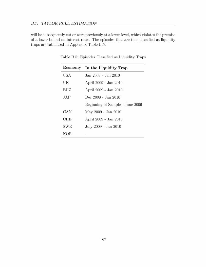
B.7. TAYLOR RULE ESTIMATION
will be subsequently cut or were previously at a lower level, which violates the premiseof a lower bound on interest rates. The episodes that are thus classified as liquiditytraps are tabulated in Appendix Table B.5.
Table B.5: Episodes Classified as Liquidity Traps
Economy In the Liquidity Trap
USA Jan 2009 - Jan 2010
UK April 2009 - Jan 2010
EUZ April 2009 - Jan 2010
JAP Dec 2008 - Jan 2010
Beginning of Sample - June 2006
CAN May 2009 - Jan 2010
CHE April 2009 - Jan 2010
SWE July 2009 - Jan 2010
NOR -
197

B.7.
TAYLOR
RULEESTIM
ATIO
N
Table B.6: Taylor rule estimates
(1) (2) (3) (4) (5) (6) (7)
USA UK EUZ CAN CHE SWE NOR
Lagged Interest Rate 0.931∗∗∗ 0.973∗∗∗ 0.846∗∗∗ 0.914∗∗∗ 0.905∗∗∗ 0.938∗∗∗ 0.958∗∗∗
(0.0410) (0.0404) (0.0808) (0.0510) (0.0397) (0.0373) (0.0764)
Inflation Forecast 0.275∗∗∗ 0.150 0.175 -0.0717 -0.0585 0.303∗∗∗ 0.239∗∗
(0.0813) (0.110) (0.187) (0.141) (0.0895) (0.0555) (0.117)
Growth Forecast 0.234∗∗∗ 0.302∗∗∗ 0.349∗∗∗ 0.299∗∗∗ 0.425∗∗∗ 0.222∗∗∗ 0.107
(0.0642) (0.0701) (0.0831) (0.102) (0.0716) (0.0504) (0.190)
Contemporaneous Output Gap 0.119∗∗ 0.0861 0.0229 0.0502 -0.0729 0.0117 0.156∗∗
(0.0463) (0.0526) (0.0812) (0.0730) (0.0429) (0.0278) (0.0698)
Constant -1.114∗∗∗ -0.834∗∗∗ -0.587 -0.369 -0.571∗∗∗ -0.904∗∗∗ -0.760
(0.275) (0.265) (0.388) (0.526) (0.150) (0.201) (0.840)
Observations 63 42 35 63 35 53 38
R2 0.968 0.970 0.969 0.819 0.967 0.978 0.932
Robust standard errors in parentheses
∗ p < 0.1, ∗∗ p < 0.05, ∗∗∗ p < 0.01
198

B.7. TAYLOR RULE ESTIMATION
Figure B.4: Predicted Policy Rates from Taylor Rule Estimates
-4
-4
-4-2
-2
-20
0
02
2
24
4
46
6
61992q1
1992q1
1992q11996q3
1996q3
1996q32001q1
2001q1
2001q12005q3
2005q3
2005q32010q1
2010q1
2010q1time
time
timeInterest Rate
Interest Rate
Interest RatePredicted Values
Predicted Values
Predicted Values
(a) USA
-5
-5
-50
0
05
5
510
10
101992q1
1992q1
1992q11996q3
1996q3
1996q32001q1
2001q1
2001q12005q3
2005q3
2005q32010q1
2010q1
2010q1time
time
timeInterest Rate
Interest Rate
Interest RatePredicted Values
Predicted Values
Predicted Values
(b) UK
-4
-4
-4-2
-2
-20
0
02
2
24
4
41992q1
1992q1
1992q11996q3
1996q3
1996q32001q1
2001q1
2001q12005q3
2005q3
2005q32010q1
2010q1
2010q1time
time
timeInterest Rate
Interest Rate
Interest RatePredicted Values
Predicted Values
Predicted Values
(c) EUZ
-2-2
-200
022
244
466
688
81992q1
1992q1
1992q11996q3
1996q3
1996q32001q1
2001q1
2001q12005q3
2005q3
2005q32010q1
2010q1
2010q1time
time
timeInterest Rate
Interest Rate
Interest RatePredicted Values
Predicted Values
Predicted Values
(d) CAN
-4
-4
-4-2
-2
-20
0
02
2
24
4
41992q1
1992q1
1992q11996q3
1996q3
1996q32001q1
2001q1
2001q12005q3
2005q3
2005q32010q1
2010q1
2010q1time
time
timeInterest Rate
Interest Rate
Interest RatePredicted Values
Predicted Values
Predicted Values
(e) CHE
0
0
010
10
1020
20
2030
30
3040
40
401992q1
1992q1
1992q11996q3
1996q3
1996q32001q1
2001q1
2001q12005q3
2005q3
2005q32010q1
2010q1
2010q1time
time
timeInterest Rate
Interest Rate
Interest RatePredicted Values
Predicted Values
Predicted Values
(f) SWE
199