Macroeconomic Determinants of International Housing Markets

ABSTRACT

This paper examines the long-term impact and short-term dynamics of macroeconomic

variables on international housing prices. Since adequate housing market data are generally

not available and usually of low frequency, a panel cointegration analysis consisting of 15

countries over a period of thirty years is applied. Pooling the observations allows us to

overcome the data restrictions which researchers face when testing long-term relationships

among single real estate time series. This study does not only confirm results from previous

studies but also allows for a comparison of single country estimations in an integrated

equilibrium framework. The empirical results indicate positive effects on house prices

arising from an increase in economic activity, construction costs, and the short-term interest

rate and negative effects stemming from an increase in the long-term interest rate. Deviations

from the long-term equilibrium result in a dynamic adjustment process that can take several

years.

Keywords: Housing market, macroeconomy, panel cointegration, FMOLS, DOLS

JEL-Classification: C33, G15

1. Introduction

In the past, long-run equilibrium models of housing markets and the macroeconomy have been

restricted to countries that offer a high availability of long time series of housing market data.

The reason for this is that cointegration techniques such as the Engle-Granger or the Johansen

approach require a sufficiently large time period in order to test on long-run relationships.

Accordingly, such studies so far have been restricted to the US (Catte 2004, Case 2000), the UK

(Meen 1996, Bowen 1994) and a few other countries.1 To overcome this restriction this study

uses macroeconomic and housing market data from 15 OECD countries and applies the panel

cointegration approach proposed by Pedroni (1999, 2000, 2004). This method makes use not

only of the T observations of a time series of a single country but pools the observable data over

all N countries so that in effect real observations are available for estimation. This results

in a higher robustness of the estimation process since the effects of large sample asymptotics are

more likely to apply in this environment. The main advantage however lies in the existence of an

international housing market result which can be obtained by weighting the individual country

estimations. Finally, in recent literature variables of panel data were found to be cointegrated

even where there was no cointegration between them in individual time series. Hence, this study

does not only confirm results from earlier studies but also highlights the differences between

countries in an integrated long-run equilibrium framework.

N T⋅

The study is organized as follows: the next section discusses a theoretical long-run

equilibrium model of the housing market which is used as a theoretical foundation for the

empirical investigation. Section three applies the panel cointegration technique for non-

stationary panel data which is used to test and estimate long-term equilibrium relationships

between the housing market and macroeconomic variables. Furthermore, an error correction 1 For a recent and comprehensive literature overview see Leung (2004).

2

model is estimated to describe the adjustment process to this long-term equilibrium. Some

conclusions are drawn in section four.

2. Macroeconomic Effects and their propagation mechanism on the Housing Market

In contrast to other capital market assets, real estate prices do not change immediately after

economic news has been released and generally exhibit low price fluctuation. Residential

housing prices in particular show strong downward price stickiness since house owners have

high reservation prices or simply resist to sell their house under a certain price during recessions.

Price inertia, however, also influences the behaviour of housing prices during economic booms

since exuberant expectations of house owners facilitate the formation of housing bubbles.2 The

propagation of macroeconomic shocks on US house prices have been discussed in the literature,

e.g. Catte (2004) and Case (2000). Macroeconomic shocks such as unexpected changes in the

money supply, industrial production or changes in the interest rate effect house prices with a lag

depending on the speed of the propagation mechanism. The speed of propagation is determined

by the efficiency of the institutional framework such as zoning regulations, the speed of

administrative processes, credit supply, transaction costs or the mortgage market. If for example

changes in the interest rates propagate quickly into changes of mortgage market interest rates,

then an increase in the money supply affects the housing market more quickly compared to a

situation where most mortgage rates are fixed and the mortgage market in general is inefficient.

The credit supply for housing financing can also vary between countries depending on the real

estate valuation methods. If the valuation method reacts sensitively to changes in real estate

2 Furthermore, price information in the real estate market is often limited and inaccurate as real estate is sold only

infrequently and information about prices is often specific to the respective local market. For this reason, price

forecasts are usually simple extrapolations from the past. This leads to endogeneous dynamics of real estate prices

and thus facilitates the formation of housing bubbles. The contribution of those endogeneous dynamics can be

substantial and varies between 70 % and 40 % depending on the country under consideration (Zuh 2003).

3

prices and if the loan-to-value (LTV) ratio3 is high, rising house prices increase the credit supply

more strongly and vice versa, decreasing house prices lead to a shortage in the credit supply. A

higher credit supply in turn increases the importance of interest rate changes as more firms and

households rely on debt financing. Lower transaction costs on the other hand lead to more

transactions and thus to a faster response of house prices in face of a macroeconomic shock.

Furthermore, housing supply inelasticities lead to a stronger weight on price reactions relative to

supply reactions.

However, there might also be a feedback reaction from housing prices to the

macroeconomy. Rising house prices make homeowners feel richer.4 The value of their houses

increases, and thus, the size of the collateral that people can borrow on. For liquidity constrained

households, an increase in house price may be the only opportunity to borrow at all. This wealth

effect then increases consumption. A decline in house prices leads to a negative effect on

consumption since decreasing house prices lead to more mortgage defaults and thus reduce the

supply of bank credit as banks loose part of their bank capital (Parker 2000). Here, the mortgage

market also plays an important role for the propagation of real house prices to the

macroeconomy. Higher mortgage debt means a higher leverage through which changes in the

interest rate can affect consumer spending. The effect of house prices on consumption is

especially strong in the US as shown in Case (2000), where two thirds of all occupants are also

owner-occupants so that the wealth effect has a strong impact on consumer spending.5 Real

3 Loan-to-value (LTV) is defined as ratio of the value of the loan to the value of the collateral. 4 For instance, in the United States, about two thirds of the population are house owners. The increase in house

prices is of course disadvantageous for the other one third of the population who rent houses as rents increase as

well. 5 Case et al. (2005) show that the consumption effect of housing wealth is even larger than the effect stemming from

financial wealth.

4

house prices even have a stronger effect on consumption than stock market prices which might

be due to the fact that house ownership is more evenly distributed across households than stock

market wealth. Stock market wealth is mainly held by rich households and since the propensity

to consume declines with increasing wealth, an increase in house prices has a stronger effect on

consumption than an increase in stock prices.6

Global macroeconomic effects on real estate prices have been discussed in Case (2000).

Real estate markets appear to show high correlations internationally even though they are not

substitutes since they are bound to a specific place. However, fundamentals like GDP which

drive real estate markets are internationally correlated.7 The strength of those global factors

depend on the openness of the country and GDP correlations were found to range on average

between 0.33 and 0.44 (Case 2000).8

The slow propagation of macroeconomic effects on the one hand and endogenous

feedback effects on the other hand ask for a long-run equilibrium analysis and a model of short-

run dynamics to model deviations from this long-run equilibrium.

In order to provide a theoretically based motivation for our choice of variables in the

empirical part of this study we briefly present a simple supply and demand model. In this

context, we build on the theoretical equilibrium model of DiPasquale and Wheaton (1996).

Central to this model in Figure 1 is the distinction between the asset and the property market as

well as their interaction:9

6 Some economists, however, do not believe in the existence of such wealth effects, see e.g. Glaeser (2000). 7 The real estate crash of office prices in the early 1990s e.g. was felt by nearly every country around the world. 8 Other, non-macroeconomic effects have been studied as well. See e.g. Parker (2000) for the effect of population

growth on house prices and Cocco (2005) for real estate in the portfolio context. 9 For a more detailed discussion the reader is referred to DiPasquale and Wheaton (1996).

5

One the one side is the asset market which determines the price of real estate and leads to

an equilibrium of the demand to own houses, and the supply of houses. The supply of houses

depends on house prices relative to the construction costs of building a new house. Since one

important aspect of real estate is its short-term inelasticity of supply, a sudden increase in

demand will increase prices. For given construction costs, this increase in the price acts as an

incentive for investors to build new houses until the price decreases to its long-term relation of

replacement costs and the costs of land, at which point the investor has no incentive to build

more houses. The demand to own houses depends negatively on house prices but positively on

the rental income that houses earn as an asset.

On the other side is the property market which equates demand and supply of real estate

and housing use or space. Individuals, whether owners or tenants , require space for living. For a

tenant, space is part of overall consumption spending and the demand for space, i.e. the use of

real estate, depends on the rent relative to the price of other consumer goods and on economic

factors like disposable income. For a house owner, the rents are the annualized opportunity costs

of using the space instead of renting it to other individuals. The supply of real estate space is

given by the asset market. The rent is determined by the property market where demand for

space equals supply of space. For a given inelastic supply, an increase in economic activity, e.g.

an increase in household’s disposable income or a higher level of production, lead to higher

rents.

<< Figure 1 about here >>

Within this framework we implement the following long-run model of supply and

demand:

(1) D Dt t tD x z tα β δ ε′ ′= + + +

6

Dtx is a vector of macroeconomic variables affecting demand and D

tz is a vector of country-

specific factors affecting housing demand on the micro level such as mortgage market

characteristics, tax regulations, and depreciation laws. Since we focus in this study on the

macroeconomic impacts on housing markets the vector Dtz is incorporated in the error term and

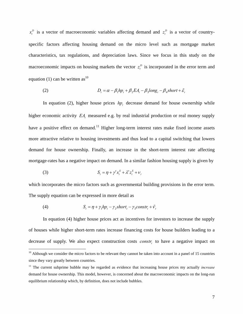
equation (1) can be written as10

(2) 1 2 3 4t t t tD hp EA long short tα β β β β ε= − + − − +

In equation (2), higher house prices decrease demand for house ownership while

higher economic activity measured e.g. by real industrial production or real money supply

have a positive effect on demand.

thp

tEA

11 Higher long-term interest rates make fixed income assets

more attractive relative to housing investments and thus lead to a capital switching that lowers

demand for house ownership. Finally, an increase in the short-term interest rate affecting

mortgage-rates has a negative impact on demand. In a similar fashion housing supply is given by

(3) S St t tS x z tη γ λ′ ′ ν= + + +

which incorporates the micro factors such as governmental building provisions in the error term.

The supply equation can be expressed in more detail as

(4) 1 2 3t t t tS hp short constr tη γ γ γ= + − − +ν

decrease of supply. We also expect construction costs to have a negative impact on

In equation (4) higher house prices act as incentives for investors to increase the supply

of houses while higher short-term rates increase financing costs for house builders leading to a

tconstr

10 Although we consider the micro factors to be relevant they cannot be taken into account in a panel of 15 countries

since they vary greatly between countries. 11 The current subprime bubble may be regarded as evidence that increasing house prices my actually increase

demand for house ownership. This model, however, is concerned about the macroeconomic impacts on the long-run

equilibrium relationship which, by definition, does not include bubbles.

7

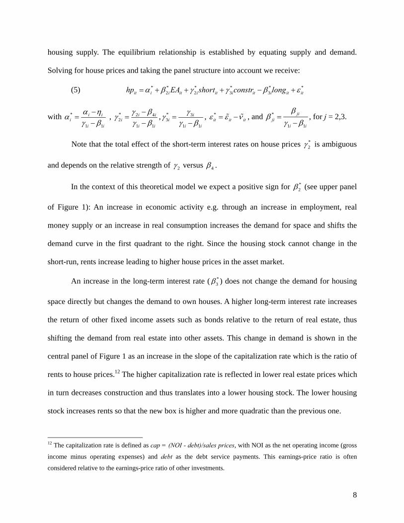
housing supply. The equilibrium relationship is establis equating supply and demand.

Solving for house prices and taking the panel structure into account we receive:

(5) * * * * * *2 2 3 3it i i it i it i it i it ithp EA short constr long

hed by

α β γ γ β ε= + + + − +

*with 1 1

i ii

i i

α ηαγ β

−−

, = * 2 42

1 1

i ii

i i

γ βγγ β

−=

−, * 3

31 1

ii

i i

γγγ β

=−

, *it it itε ε ν= − , and *

1 1

jiji

i i

ββ

γ β=

−, for j = 2,3.

Note that th l effect of est rates on house prices e tota the short-term inter * is ambiguous2γ

and depends on the relative strength of 2γ versus 4β .

In the context of this theoretical odel we xp m e ect a positive sign for *2β (see upper panel

of Figure 1): An increase in economic activity e.g. through an increase in employment, real

money supply or an increase in real consumption increases the demand for space and shifts the

demand curve in the first quadrant to the right. Since the housing stock cannot change in the

short-run, rents increase leading to higher house prices in the asset market.

An increase in the long-term interest rate ( *3β ) does not change the demand for housing

space d es

stock increases rents so that the new box is higher and more quadratic than the previous one.

irectly but changes the demand to own hous . A higher long-term interest rate increases

the return of other fixed income assets such as bonds relative to the return of real estate, thus

shifting the demand from real estate into other assets. This change in demand is shown in the

central panel of Figure 1 as an increase in the slope of the capitalization rate which is the ratio of

rents to house prices.12 The higher capitalization rate is reflected in lower real estate prices which

in turn decreases construction and thus translates into a lower housing stock. The lower housing

12 The capitalization rate is defined as cap = (NOI - debt)/sales prices, with NOI as the net operating income (gross

income minus operating expenses) and debt as the debt service payments. This earnings-price ratio is often

considered relative to the earnings-price ratio of other investments.

8

The third effect, which is likely to have an impact on the supply schedule of new

construction is a change in the short-term interest rate or in the construction costs. Higher short-

term in

short-term interest rate making the theoretical outcome more

compli

irst, we test the

onarity using panel unit-root tests. Afterwards, we apply panel cointegration

tests to detect the long-term equilibrium relationships, and finally we estimate the short-term

terest rates and generally all factors that increase the costs of construction such as an

increase in the price of construction materials or stricter building regulations increase the

financing costs of construction. This effect is shown in the bottom panel of Figure 1 as a shift of

the construction line to the left. The higher construction costs lead to a decrease in construction

and thus to a lower level of the housing stock. The lower housing stock also means less housing

space which increases rents. Higher rents then generate higher house prices in the asset market.

As evident, the location of the new box is higher and more to the left relative to the previous box.

Rents and house prices are higher but construction and the housing stock are lower than without

the increase in the short-term interest rate. The exact position of the box depends on the

elasticities of the individual curves.

In reality, the effects described above often occur at the same time, e.g. an increase in

economic activity also increases the

cated. Furthermore, the model is a static equilibrium model, whereas the propagation of

the various effects would also be interesting to investigate. In the next section we apply a panel

cointegration approach with the associated error correction model for modeling long-run

equilibria and the corresponding short-run dynamics.

4. Long-Term Equilibrium Relationships between Housing Markets and the

Macroeconomy

Cointegration analysis for non-stationary panel data is conducted in three steps: F

variables for stati

9

dynamics.13 For the following estimation, house prices for fifteen countries ranging from

1975Q1 to 2007Q2 are used. The 15 countries are Australia, Belgium, Canada, Denmark,

Finland, France, Ireland, Italy, Netherlands, New Zealand, Norway, Spain, Sweden, the UK, and

the USA.14 Figure 2 shows the development of the log real house prices since 1975.15

<< Figure 2 about here >>

4.1 Panel Unit Root Tests

Early work on non-stationary panel data include Quah (1994) or Levin and Lin (1993) who study

unit root tests under the null hypot ing homogeneous parameters of

riable. Im, Pesaran and Shin (1997) and Maddala and Wu (1999)

hesis of non-stationarity assum

the lagged endogenous va

propose unit root tests which also allow for heterogeneous autoregressive roots. The Levin and

Lin (LL) test, the Im, Pesaran and Shin (IPS) test and the Fisher Phillips-Perron (Fisher-PP) test

have been the most popular in the literature (see Maddala and Wu 1999). The main drawback of

the LL test is that the autoregressive root ρ is assumed to be the same for all i :

0...:0 21 ===== ρρρρ NH against the alternative hypothesis

0...:1 <==== 21 ρρρρ N

Although the LL test allows for heterogeneity in the variance and serial correlation

structure of the error terms, the restricti o clearly too strong

and the alternative hypothesis is thus of no practical interest. The IPS test in contrast is a

generalization of the LL test that combines the test statistics of the individual unit root tests for

H

on f homogeneous slope parameters is

13 Cointegration methodology for testing long-term equilibrium relationships between single time series have been

developed by Engle and Granger (1987) for the univariate case and by Johansen and Juselius (1990) for the

multivariate case. 14 Germany and Japan were excluded from the data set due to inaccurate housing price data. 15 Although we are aware of the potential impact of the housing bubble on our analysis, we decided to include the

recent years in order to include recent relevant information and to increase the total number of observations.

10

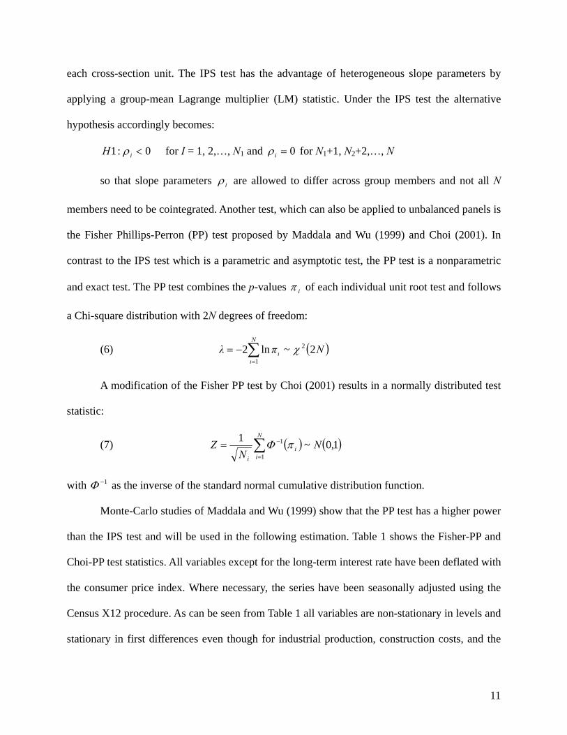
each cross-section unit. The IPS test has the advantage of heterogeneous slope parameters by

applying a group-mean Lagrange multiplier (LM) statistic. Under the IPS test the alternative

hypothesis accordingly becomes:

0:1 <iH ρ for I = 1, 2,…, N1 and 0=iρ for N1+1, N2+2,…, N

so that slope parameters iρ are allowed to differ across group members and not all N

members need to be cointegrated. Another test, which can also be applied to unbalanced panels is

the Fisher Phillips-Perron (PP) test proposed by Maddala and Wu (1999) and Choi (2001). In

contrast to the IPS and a etric

and exa

test which is a parametric symptotic test, the PP test is a nonparam

ct test. The PP test combines the p-values iπ of each individual unit root test and follows

a Chi-square distribution with 2N degrees of freedom:

Ν

ι

2

1

(6) ι 2~ln2 χ∑ ( )Nπλ=

−=

A modification of the Fisher PP test by Choi (2001) results in a normally distributed test

statistic:

( ) ( )1(7) ,0~11

1 NN

ZN

ii

i∑=

−= πΦ

with 1−Φ as the inverse of the standard normal cumulative distribution function.

Monte-Carlo studies of Maddala and Wu (1999) show that the PP test has a higher power

than the IPS test and will be used in the following estimation. Table 1 shows the Fisher-PP and

Choi-PP test statistics. All variables except for the long-term interest rate have been deflated with

justed using the

Census

the consumer price index. Where necessary, the series have been seasonally ad

X12 procedure. As can be seen from Table 1 all variables are non-stationary in levels and

stationary in first differences even though for industrial production, construction costs, and the

11

interest rates the evidence of a unit root is rather weak. The fact that almost all variables seem to

be stationary when considering both individual intercepts and individual trends seems puzzling.

When tested individually, the variables are non-stationary. Furthermore, Pedroni (2000) suggests

omitting the individual trends and only to include individual intercepts. After concluding that the

variables are integrated of order 1, I(1) in levels but I(0) in differences, the next step is to test if a

cointegration relationship between the variables exists.

<< Table 1 about here >>

4.2. Panel Cointegration Test

If the macroeconomic and housing market variables are I(1) but a linear relationship between

those variables is I(0), the variables are cointegrated. In order to test for cointegration, a

cointegration test for heterogeneou sors developed by Pedroni (2000)

ll hypothesis of no cointegration and also allows for unbalanced

s panels with multiple regres

is applied. This test has the nu

panels. In this test the regression residuals are computed from the following regression:

(8) titMiMitiitiiiiti exxxty ,,,22,11, ... +⋅++⋅+⋅++= ρρρδα

for t = 1,…, T ; I = 1,…, N ; m = 1,…, M

with individual fixed effects iα and individual time trend tiδ , although such individual

time trends are often omitted. In some cases common time dummies can also be included.16 In

this equation, m regressors are allowed and the slope coefficients tmix , miρ and thus the

cointegration vectors are heterogeneous for all i. The residuals from equation (8) are then

tested on unit roots:

(9)

tie ,

titiiti ee ,1,, ˆˆ ερ += −

16 In the following analysis time dummies have not been subtracted since common time effects are almost certainly

macroeconomic and thus directly controlled for in the model.

12

Including fixed effects and time trends changes the asymptotic distribution and increases

the critical values of the unit root statistic. This is because in the presence of a unit root, the

sample average of a variable with a stochastic trend ∑=

=T

ttii y

Ty

1,

1 does not converge to the

population mean with increasing T.17 In Pedroni (1999) seven test statistics are proposed. For our

purpose

in the case of

hypothesis of cointegration. Pedroni (2000, 2004) shows that under general requirements the test

short-term and the long-term interest rate, and construction costs.

we decided to use the multivariate extensions of the Phillips-Perron Roh (PPr) and

Phillips-Perron t (PPt) statistic which are both nonparametric and do not require the slope

coefficients of the regression residuals to be homogeneous for all the alternative

statistics follow a normal distribution as T and N grow large. We test two models, both include

supply and demand variables but focus on different aspects of the theoretical model.

i

18 The

smaller model (model I) tests on cointegration between house prices, industrial production as

well as short-run and long-run interest rates. This model therefore concentrates on the

relationships of the two interest rates. The second model (model II) confirms the effects of

economic activity by including money supply and employment as economic activity variables

but also includes the long-run interest rate and construction costs. Table 2 shows the

cointegration test results from the PPr and PPt test.

<<Table 2 about here >>

All values are larger than 1.65 so that the null hypothesis of no cointegration is rejected

and house prices are cointegrated with the industrial production, money supply, employment, the

17 In fact, it can be shown that the sample mean diverges at a rate T . 18 Our experience was that the regression estimations below produce bad results for more than 4 variables.

Multicollinearity, which is strong e.g. between economic activity variables such as industrial production and money

supply may be a reason.

13

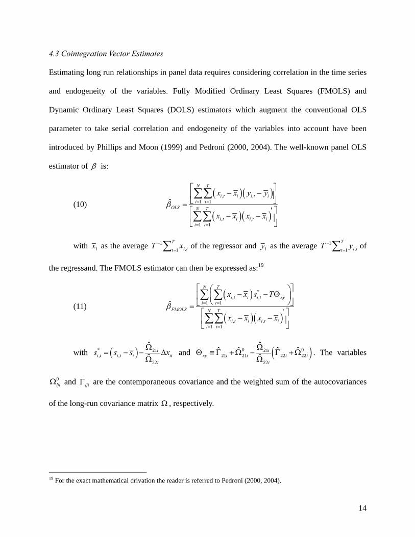
4.3 Cointegration Vector Estimates

Estimating long run relationships in panel data requires considering correlation in the time series

and endogeneity of the variables. Fully Modified Ordinary Least Squares (FMOLS) and

Dynam

). The well-known panel OLS

ic Ordinary Least Squares (DOLS) estimators which augment the conventional OLS

parameter to take serial correlation and endogeneity of the variables into account have been

introduced by Phillips and Moon (1999) and Pedroni (2000, 2004

estimator of β is:

( )( )

( )( )

, ,1 1

, ,1 1

ˆ

N T

i t i i t ii t

OLS N T

i t i i t ii t

(10) x x y y

x x x xβ = =

= =

⎡ ⎤− −⎢ ⎥

⎣ ⎦=′⎡ ⎤

− −⎢ ⎥⎣ ⎦∑∑

with

∑∑

ix as the average ∑− T xT 1 of the regressor and =t ti1 , iy as the average ∑− T yT 1 of

19

=t ti1 ,

the regressand. The FMOLS estimator can then be expressed as:

(11) ( )

( )( )

*, ,

1 1

, ,1 1

ˆ

N T

i t i i t xyi t

FMOLS N T

i t i i t ii t

x x s T

x x x xβ = =

= =

⎡ ⎤⎛ ⎞− − Θ⎢ ⎥⎜ ⎟

⎝ ⎠⎣ ⎦=′⎡ ⎤

− −⎢ ⎥⎣ ⎦

∑ ∑

∑∑

with ( )* 21, , ˆi t i t is s= − −

Ω

22

ˆi

iti

s xΩ∆ and ( )0 021

21 21 22 22ˆxy i i i ii

Θ ≡ Γ +Ω − Γ +ΩΩ

. T

0ljiΩ and ljiΓ are the contemporaneous covariance and the weight

22

ˆˆ ˆˆ ˆiΩ he variables

ed sum of the autocovariances

of the long-run covariance matrix , respectively.

Ω

19 For the exact mathematical drivation the reader is referred to Pedroni (2000, 2004).

14

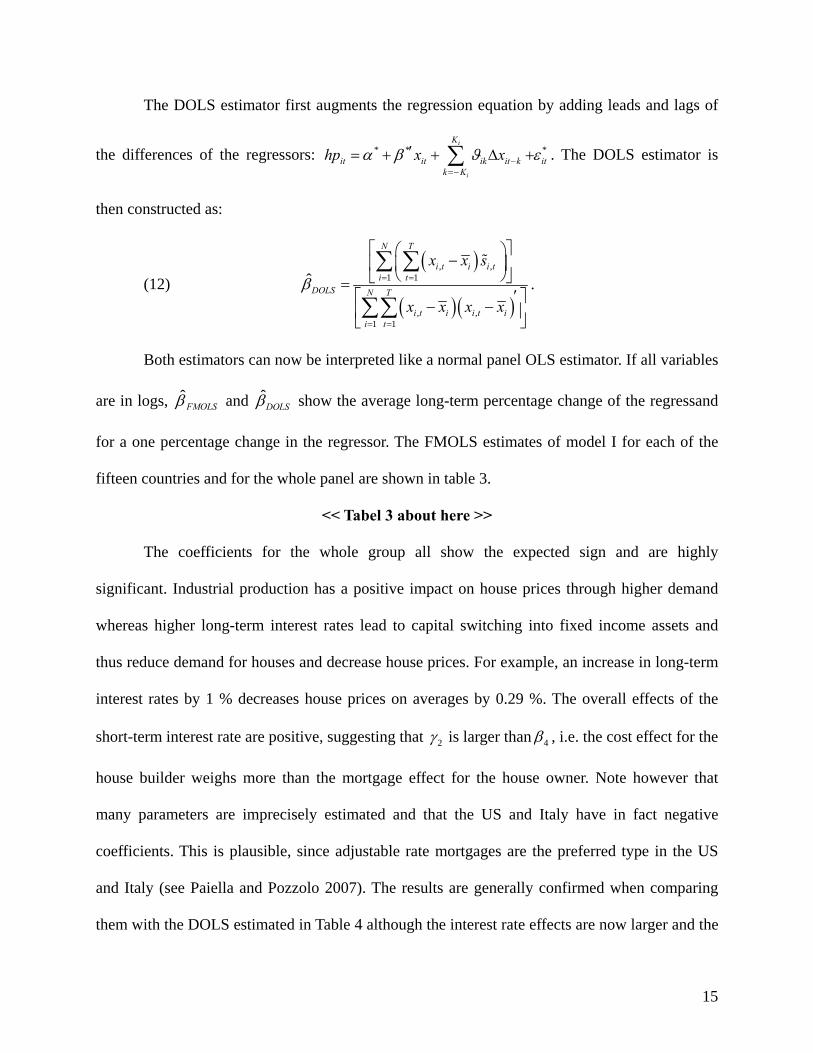
The DOLS estimator first augments the regression equation by adding leads and lags of

the differences of the regressors: *K

it it ik it k ithp x x* *i

ik K

α β ϑ ε−′

=−

= + + ∆ +∑ . The DOLS estimator is

(12)

then constructed as:

( )

( )( )

, ,

N T

i t i i tx x s1 1

, ,1 1

ˆ i tDOLS N T

i t i i t ii t

x x x xβ = =

= =

⎡ ⎤⎛ ⎞−⎢ ⎥⎜ ⎟

⎝ ⎠⎣ ⎦=′⎡ ⎤

− −⎢ ⎥⎣ ⎦∑∑

.

rs can now be interpreted like a normal panel OLS estimator. If all variables

are in logs, and

∑ ∑

Both estimato

FMOLSβ ˆDOLSβ show the average long-term percentage change of the regressand

for a one percentage change in the regressor. The FMOLS estimates of model I for each of the

fifteen countries and for the whole panel are shown in table 3.

coeffic for

ing into fixed income assets and

thus reduce demand for houses and example, an increase in long-term

interest

<< Tabel 3 about here >>

The ients the whole group all show the expected sign and are highly

significant. Industrial production has a positive impact on house prices through higher demand

whereas higher long-term interest rates lead to capital switch

decrease house prices. For

rates by 1 % decreases house prices on averages by 0.29 %. The overall effects of the

short-term interest rate are positive, suggesting that 2γ is larger than 4β , i.e. the cost effect for the

house builder weighs more than the mortgage effect for the house owner. Note however that

many parameters are imprecisely estimated and that the US and Italy have in fact negative

coefficients. This is plausible, since adjustable rate mortgages are the preferred type in the US

and Italy (see Paiella and Pozzolo 2007). The resul are generally nfirmed when comparing

them with the DOLS estimated in Table 4 although the interest rate effects are now larger and the

ts co

15

impact of industrial production appears to be very low. The panel group results for the DOLS

estimates are not the averages of the individual results as in the case of the FMOLS method but

are weighted by the precision of its estimate, thus giving more weight to the more stable

estimates.

<< Table 4 about here >>

In Table 5, economic activity measured by money supply and employment have much

higher effects on housing prices compared to model I. Instead of the monetary costs from

increasing short-term interest rates we now model the costs of labor and material by the

construction cost index.

seen in Table 6 which shows the DOLS results of model II. Except for

the interest rate effect of -0.36 wh ms than the FMOLS estimates of

-0.05, a

4.4 Err

ng it would take for the housing market to reach the equilibrium

position e it has deviated from equilibrium due to an exogeneous shock to the economy. For

<< Table 5 about here >>

As expected, an increase in construction costs leads to an increase in house prices as the

supply of houses decreases. The effects of the long-term interest rate are somewhat lower than in

model I. This can also be

ich is larger in absolute ter

ll other parameters are estimated somewhat lower than in the FMOLS equation.

<< Table 6 about here >>

Despite the differences in parameter values between methods, model specifications, and

individual countries the overall performance is satisfying and the theoretical model is strongly

supported by all four models.

or Correction Model

After having analyzed the long run impact of the macroeconomic variables on the housing

market, one could ask how lo

onc

16

this reason, an Error Correction Model (ECM) which models the adjustment process to

Where the

equilibrium has been estimated. The deviations from the equilibrium can be expressed as:

(13) 11 2 3it it it it itecm hp rip short longβ β β= − − − (model I)

(13)’ 2ecm hp rmoney employ constr longδ δ δ δ= − − − − (model II) 1 2 3 4it it it it it it

iβ and the iδ are the corresponding FMOLS and DOLS parameter estimates

of model I and model II, respectively. If the variables are in equilibrium, the error correction

term is zero. If the variables deviate from equilibrium, for example if the house prices

are too high relative to their equilibrium position, then the error term is positive. In this situa

w

s.20 S les

14 log log log log 1it i ij it j in it n is it shp hp prod short− −

jitecm ithp

tion,

ithp ill decrease in the following periods until the equilibrium is reached. This adjustment

process can be estimated by including the lagged error term in a panel regression with random

effect ince the panel regression has to be estimated with stationary variables, all variab

except the error term are included as dlogs:

( ) ( )1 0 0

ˆ ˆ ˆ ˆK N S

j n sα α α α0 1 2 3 −

= = =

∆ = + ∆ + ∆ + ∆ +

4 5 10

M

im i it tit mm

∑ ∑ ∑

ˆ ˆlog 1 long ecm( ) 1α α ε+ ∆ + + +∑ (model I)

ˆ ˆlog logN S

it i ij it j in it n is it sj n s

hp rmoney employγ γ

−−=

( ) ˆ ˆ14 ' log logK

hp γ γ0 1 2 31 0 0

− − −= = =

+ ∆ + ∆∑ ∑

1 + (model II)

Lagged house prices can also be included on the right hand side of the equation. The

error term has to be included with lag 1 since the deviation from equilibrium in the period t-1

∆ = + ∆∑

( ) 24 5 5

0 0

ˆ ˆ ˆlog 1M P

im it m ip i it tit pm p

constr long ecm eγ γ α− −−= =

+ + + +∑ ∑

ithp

20 Individual effects αi represent country specific regulatory variables and mortgage market characteristics which

can be regarded as being uncorrelated with the macroeconomic variables. Therefore, we use random effects rather

than fixed effects although for large T (130 in our case) both estimators give similar results. See Hsiao (2003).

17

starts the adjustment process in period t. The other exogeneous variables can be included in any

combination of different lag settings. Table 7 shows the error correction model for both models

and both estimation procedures.

.011 and -0.043 indicating that deviations from equilibrium are

quite persistent. Calculating the ap y

<< Table 7 about here >>

As can be seen, the error correction term has the right sign and is highly significant. If

house prices are too high reflected by a positive error term, the negative coefficient reduces

house prices in the following periods until they are in equilibrium. The value of the error term,

however, ranges only between -0

proximate adjustment time b 1 (ecm 1)− this corresponds to a

range o

also sig

30 years allows for the robust estimation of long-term macroeconomic impacts.

this context standard theoretical equilibrium models are clearly supported by the

ts and suggest that macroeconomic variables do have a significant impact on

house prices. In particular, economic activity variables such as employment, industrial

f 23 to 6 years. The long adjustment periods are probably due to the general downward

price stickiness and differences among countries may arise due to differences in micro factors.

Considering that the time period from the planning and permission stage until completion can

take quite a few years, 6 years seem to be reasonable whereas adjustment periods of more than 9

years are not. Most of the coefficients of the other variables are nificant and have the

expected sign.

5. Conclusion

This study examines the impact of the macroeconomy on house prices. Housing market data is

often not easily available or covers only short time periods. By using a panel of 15 countries over

a period of over

In

empirical resul

18

production, and money supply increase the demand for houses and thus house prices. An increase

in the short-term interest rate also affects house prices positively by increasing financing costs

and thus reducing housing construction, leading to an increase in rents and thus in house prices.

An increase in the long-term interest rate makes other fixed income assets more attractive

relative to residential property investment, reducing the demand for this kind of investment

which in turn lowers house prices.

Although the results are similar over different estimation equations and methods there is

also a high degree of variation in the findings for individual countries. This can be generally

traced back to differences that exist on the micro level such as different regulatory settings and

mortgage market characteristics. Short-run deviations from the long-run equilibrium result in

several years of adjustment until all variables are back in equilibrium.

19

References

Bowen, A. (1994), “Housing and the Macroeconomy in the United Kingdom”, Housing Policy

Debate, 5(3), 241-251.

Case, K.E. (2000), “Real Estate and the Macroeconomy”, Brookings Papers on Economic

Activity, Wellesley College.

Case, K.E., Quigley, J.M., and Shiller, R.J. (2000), “Comparing Wealth Effects: The Stock

Market versus the Housing Market.”, Advances in Macroeconomics, 5(1), 1-32.

Catte. P., N. Girouard, R. Price, and C. Andre (2004), “Housing Markets, Wealth and the

Business Cycle”, OECD Working Paper, No. 394.

Cocco, J.F. (2005), “Portfolio Choice in the Presence of Housing”, The Review of Financial

Studies, 18(2), 535-567.

Choi, I. (2001), “Unit Root Tests for Panel Data”, Journal of International Money and Finance,

20, 294-272.

DiPasquale, D., and W.C. Wheaton (1996), “Urban Economics and Real Estate Markets“,

Prentice Hall, Englewood Cliffs, New York.

Engle, R.F., and C.W.J. Granger (1987), “Co-Integration and Error-Correction: “Representation,

Estimation and Testing”, Econometrica, 55, pp. 251-276.

Glaeser, L.E. (2000), Comments and Discussion on: Case, K.E. (2000), “Real Estate and the

Macroeconomy”, Brookings Papers on Economic Activity, Wellesley College.

Hsiao, C. (2003), “Analysis of Panel Data”, 2nd ed., Cambridge University Press, Cambridge.

Im, K., H. Pesaran, and Y. Shin (1997), “Testing for Unit Roots in Heterogeneous Panels”,

Discussion Paper, University of Cambridge, June.

20

Johansen, S., and K. Juselius (1990), “Maximum Likelihood Estimation and Inference: On

Cointegration- with Applications to the Demand for Money”, Oxford Bulletin of

Economics and Statistics, 52, 162-210.

Leung, C. (2004), “Macroeconomics and Housing: a Review of the Literature”, Journal of

Housing Economics, 13, 249-267.

Levin, A., and C. Lin (1993), “Unit Root Tests in Panel Data: Asymptotic and Finite-

SampleProperties”, University of California, San Diego Discussion Paper, December.

Maddala, G..S., and S. Wu (1999), “A Comparative Study of Unit Root Tests with Panel Data and

a New Simple Test”, Oxford Bulletin of Economics and Statistics, 22, 631–652.

Meen, G. (1996), “Ten Propositions in UK Housing Macroeconomics: An Overview of the 1980s

and Early 1990s”, Urban Studies, 33(3), 425–444.

Paiella, M., and A.P. Pozzolo (2007), “Choosing between Fixed and Adjustable Rate Mortgages”,

Unpublished Working Paper at

http://papers.ssrn.com/sol3/Delivery.cfm/SSRN_ID976346

_code193151.pdf?abstractid=976346&mirid=3.

Parker, J.A. (2000), Comments and Discussion on: Case, K.E. (2000), “Real Estate and the

Macroeconomy”, Brookings Papers on Economic Activity, Wellesley College

Pedroni, P. (1999), “Critical Values for Cointegration Tests in Heterogeneous Panels with

Multiple Regressors”, Oxford Bulletin of Economics and Statistics, 22, 653-670.

Pedroni, P. (2000),”Fully Modified OLS for Heterogeneous Cointegrated Panels”, Advances in

Econometrics, 15, 93-130.

21

22

Pedroni, P. (2004), “Panel Cointegration; Asymptotic and Finite Sample Properties of Pooled

Time Series Tests, with an Application to the PPP Hypothesis”, Econometric Theory, 20,

325-597.

Phillips, P.C.B., and H. Moon (1999), “Linear Regression Limit Theory for Nonstationary Panel

Data”, Econometrica, 67, 1057-1111.

Quah, D. (1994), “Exploiting Cross-Section Variation for Unit Root Inference in Dynamic

Data”, Economics Letters, 44, 9-19.

Zuh, H. (2003), “The Importance of Property Markets for Monetary Policy and Financial

Stability”, BIS Working Paper 21.

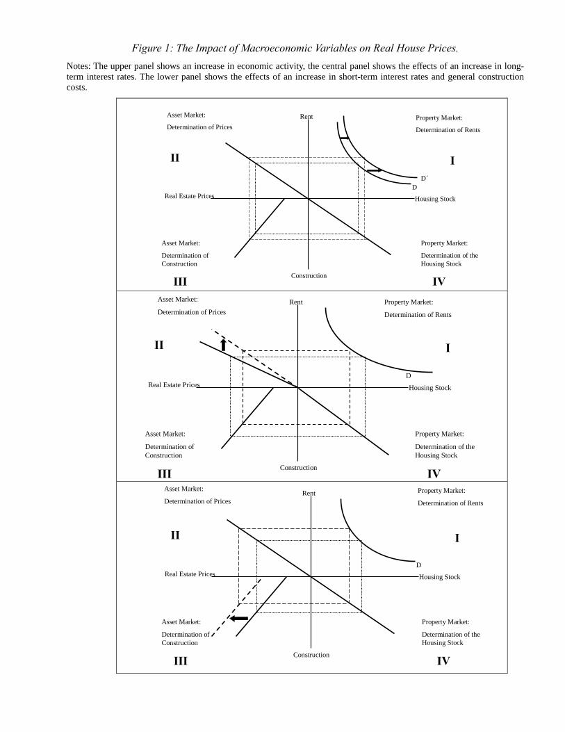
Figure 1: The Impact of Macroeconomic Variables on Real House Prices. Notes: The upper panel shows an increase in economic activity, the central panel shows the effects of an increase in long-term interest rates. The lower panel shows the effects of an increase in short-term interest rates and general construction costs.

Housing Stock

Rent

Real Estate Prices

Construction

Property Market:

Determination of Rents

Property Market:

Determination of theHousing Stock

Asset Market:

Determination of Prices

Asset Market:

Determination of Construction

DD´

III

III IV

Housing Stock

Rent

Real Estate Prices

Construction

Property Market:

Determination of Rents

Property Market:

Determination of theHousing Stock

Asset Market:

Determination of Prices

Asset Market:

Determination of Construction

D

III

III IV

Housing Stock

Rent

Real Estate Prices

Construction

Property Market:

Determination of Rents

Property Market:

Determination of theHousing Stock

Asset Market:

Determination of Prices

Asset Market:

Determination of Construction

D

III

III IV

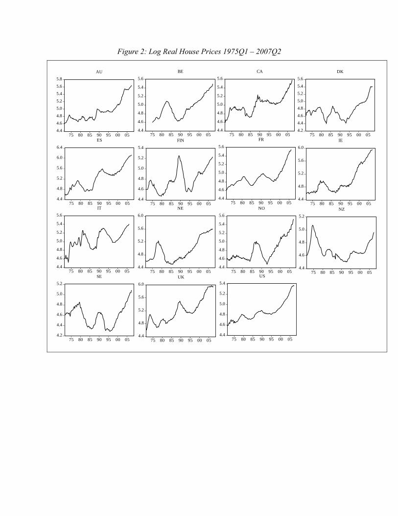
Figure 2: Log Real House Prices 1975Q1 – 2007Q2

4.4

4.6

4.8

5.0

5.2

5.4

75 80 85 90 95 00 05

US

4.4

4.6

4.8

5.0

5.2

5.4

5.6

75 80 85 90 95 00 05

FR

4.4

4.8

5.2

5.6

6.0

75 80 85 90 95 00 05

UK

4.4

4.6

4.8

5.0

5.2

5.4

5.6

75 80 85 90 95 00 05

IT

4.4

4.6

4.8

5.0

5.2

5.4

5.6

75 80 85 90 95 00 05

CA

4.4

4.8

5.2

5.6

6.0

6.4

75 80 85 90 95 00 05

ES

4.4

4.6

4.8

5.0

5.2

5.4

5.6

5.8

75 80 85 90 95 00 05

AU

4.4

4.8

5.2

5.6

6.0

75 80 85 90 95 00 05

NE

4.4

4.6

4.8

5.0

5.2

5.4

5.6

75 80 85 90 95 00 05

BE

4.2

4.4

4.6

4.8

5.0

5.2

75 80 85 90 95 00 05

SE

4.2

4.4

4.6

4.8

5.0

5.2

5.4

5.6

75 80 85 90 95 00 05

DK

4.4

4.6

4.8

5.0

5.2

5.4

5.6

75 80 85 90 95 00 05

NO

4.4

4.6

4.8

5.0

5.2

5.4

75 80 85 90 95 00 05

FIN

4.4

4.6

4.8

5.0

5.2

75 80 85 90 95 00 05

NZ

4.4

4.8

5.2

5.6

6.0

75 80 85 90 95 00 05

IE

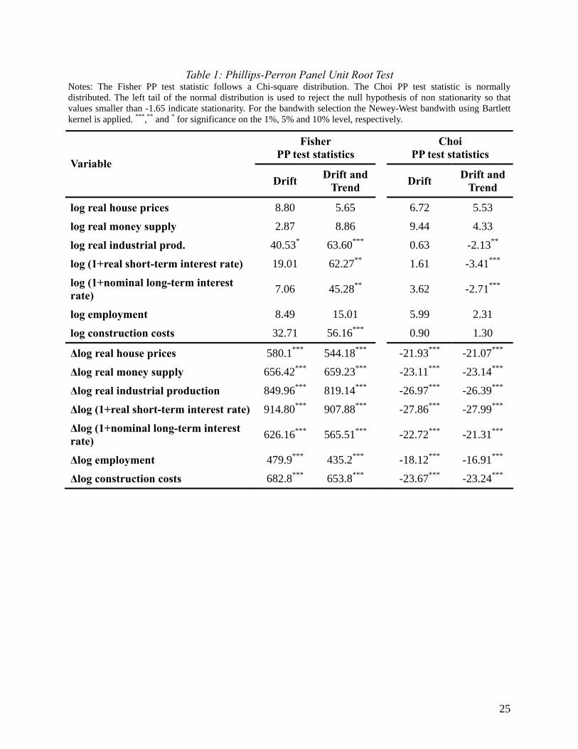
Table 1: Phillips-Perron Panel Unit Root Test Notes: The Fisher PP test statistic follows a Chi-square distribution. The Choi PP test statistic is normally distributed. The left tail of the normal distribution is used to reject the null hypothesis of non stationarity so that values smaller than -1.65 indicate stationarity. For the bandwith selection the Newey-West bandwith using Bartlett kernel is applied. ***,** and * for significance on the 1%, 5% and 10% level, respectively.

Fisher PP test statistics

Choi PP test statistics

Variable Drift Drift and

Trend Drift Drift and Trend

log real house prices 8.80 5.65 6.72 5.53

log real money supply 2.87 8.86 9.44 4.33

log real industrial prod. 40.53* 63.60*** 0.63 -2.13**

log (1+real short-term interest rate) 19.01 62.27** 1.61 -3.41***

log (1+nominal long-term interest rate) 7.06 45.28** 3.62 -2.71***

log employment 8.49 15.01 5.99 2.31

log construction costs 32.71 56.16*** 0.90 1.30

∆log real house prices 580.1*** 544.18*** -21.93*** -21.07***

∆log real money supply 656.42*** 659.23*** -23.11*** -23.14***

∆log real industrial production 849.96*** 819.14*** -26.97*** -26.39***

∆log (1+real short-term interest rate) 914.80*** 907.88*** -27.86*** -27.99***

∆log (1+nominal long-term interest rate) 626.16*** 565.51*** -22.72*** -21.31***

∆log employment 479.9*** 435.2*** -18.12*** -16.91***

∆log construction costs 682.8*** 653.8*** -23.67*** -23.24***

25

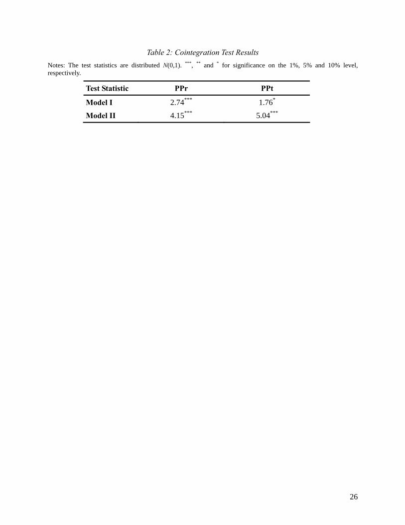
Table 2: Cointegration Test Results Notes: The test statistics are distributed N(0,1). ***, ** and * for significance on the 1%, 5% and 10% level, respectively.

Test Statistic PPr PPt

Model I 2.74*** 1.76*

Model II 4.15*** 5.04***

26

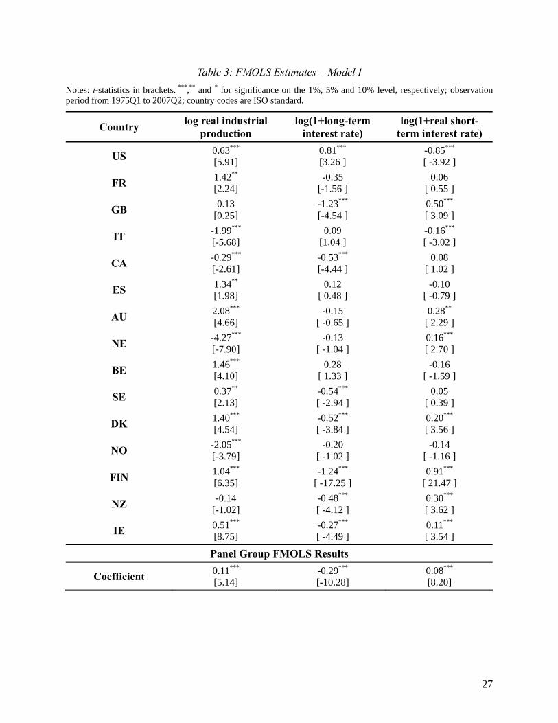
Table 3: FMOLS Estimates – Model I Notes: t-statistics in brackets. ***,** and * for significance on the 1%, 5% and 10% level, respectively; observation period from 1975Q1 to 2007Q2; country codes are ISO standard.

Country log real industrial production

log(1+long-term interest rate)

log(1+real short-term interest rate)

US 0.63*** [5.91]

0.81*** [3.26 ]

-0.85*** [ -3.92 ]

FR 1.42** [2.24]

-0.35 [-1.56 ]

0.06 [ 0.55 ]

GB 0.13 [0.25]

-1.23*** [-4.54 ]

0.50*** [ 3.09 ]

IT -1.99*** [-5.68]

0.09 [1.04 ]

-0.16*** [ -3.02 ]

CA -0.29*** [-2.61]

-0.53*** [-4.44 ]

0.08 [ 1.02 ]

ES 1.34** [1.98]

0.12 [ 0.48 ]

-0.10 [ -0.79 ]

AU 2.08*** [4.66]

-0.15 [ -0.65 ]

0.28** [ 2.29 ]

NE -4.27*** [-7.90]

-0.13 [ -1.04 ]

0.16*** [ 2.70 ]

BE 1.46*** [4.10]

0.28 [ 1.33 ]

-0.16 [ -1.59 ]

SE 0.37** [2.13]

-0.54*** [ -2.94 ]

0.05 [ 0.39 ]

DK 1.40*** [4.54]

-0.52*** [ -3.84 ]

0.20*** [ 3.56 ]

NO -2.05*** [-3.79]

-0.20 [ -1.02 ]

-0.14 [ -1.16 ]

FIN 1.04*** [6.35]

-1.24*** [ -17.25 ]

0.91*** [ 21.47 ]

NZ -0.14 [-1.02]

-0.48*** [ -4.12 ]

0.30*** [ 3.62 ]

IE 0.51*** [8.75]

-0.27*** [ -4.49 ]

0.11*** [ 3.54 ]

Panel Group FMOLS Results

Coefficient 0.11*** [5.14]

-0.29*** [-10.28]

0.08*** [8.20]

27

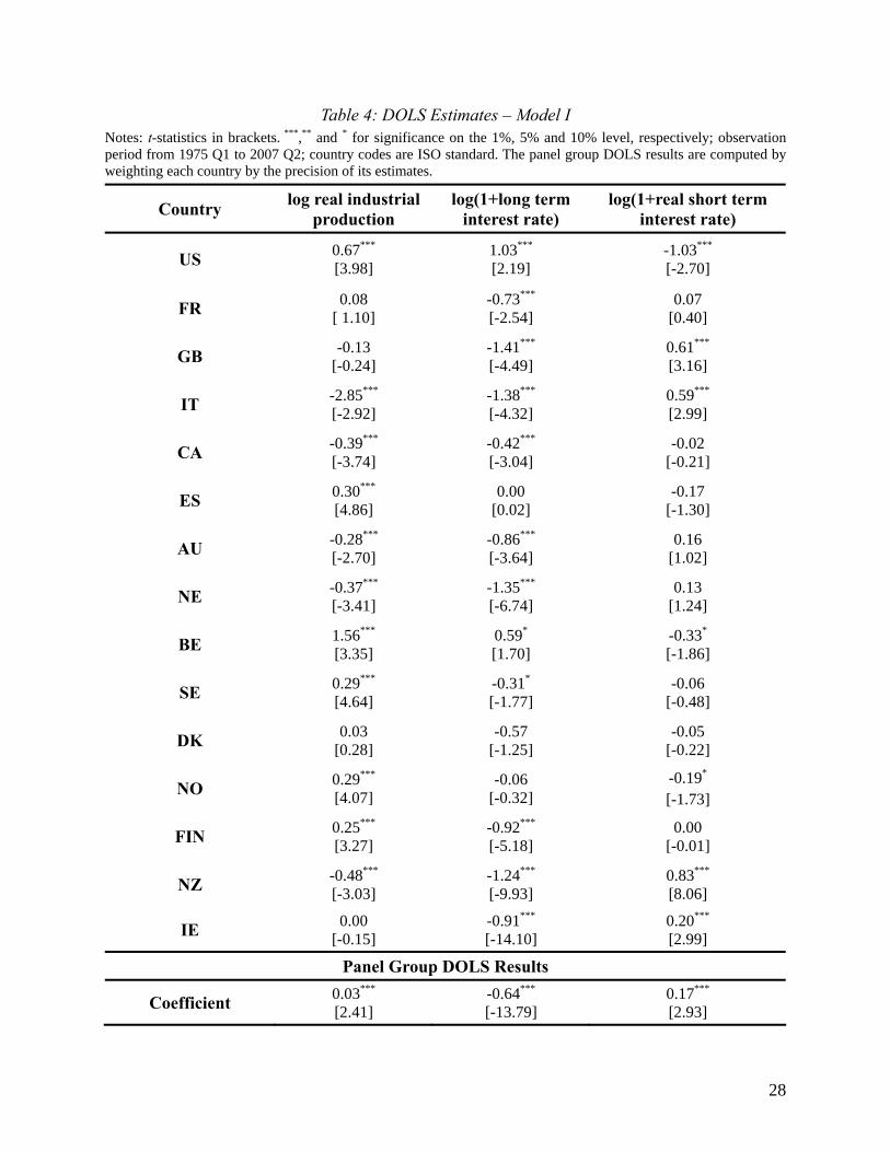
Table 4: DOLS Estimates – Model I Notes: t-statistics in brackets. ***,** and * for significance on the 1%, 5% and 10% level, respectively; observation period from 1975 Q1 to 2007 Q2; country codes are ISO standard. The panel group DOLS results are computed by weighting each country by the precision of its estimates.

Country log real industrial production

log(1+long term interest rate)

log(1+real short term interest rate)

US 0.67*** [3.98]

1.03*** [2.19]

-1.03*** [-2.70]

FR 0.08 [ 1.10]

-0.73*** [-2.54]

0.07 [0.40]

GB -0.13 [-0.24]

-1.41*** [-4.49]

0.61*** [3.16]

IT -2.85*** [-2.92]

-1.38*** [-4.32]

0.59*** [2.99]

CA -0.39*** [-3.74]

-0.42*** [-3.04]

-0.02 [-0.21]

ES 0.30*** [4.86]

0.00 [0.02]

-0.17 [-1.30]

AU -0.28*** [-2.70]

-0.86*** [-3.64]

0.16 [1.02]

NE -0.37*** [-3.41]

-1.35*** [-6.74]

0.13 [1.24]

BE 1.56*** [3.35]

0.59* [1.70]

-0.33* [-1.86]

SE 0.29*** [4.64]

-0.31* [-1.77]

-0.06 [-0.48]

DK 0.03 [0.28]

-0.57 [-1.25]

-0.05 [-0.22]

NO 0.29*** [4.07]

-0.06 [-0.32]

-0.19*

[-1.73]

FIN 0.25*** [3.27]

-0.92*** [-5.18]

0.00 [-0.01]

NZ -0.48*** [-3.03]

-1.24*** [-9.93]

0.83*** [8.06]

IE 0.00 [-0.15]

-0.91*** [-14.10]

0.20*** [2.99]

Panel Group DOLS Results

Coefficient 0.03*** [2.41]

-0.64*** [-13.79]

0.17*** [2.93]

28

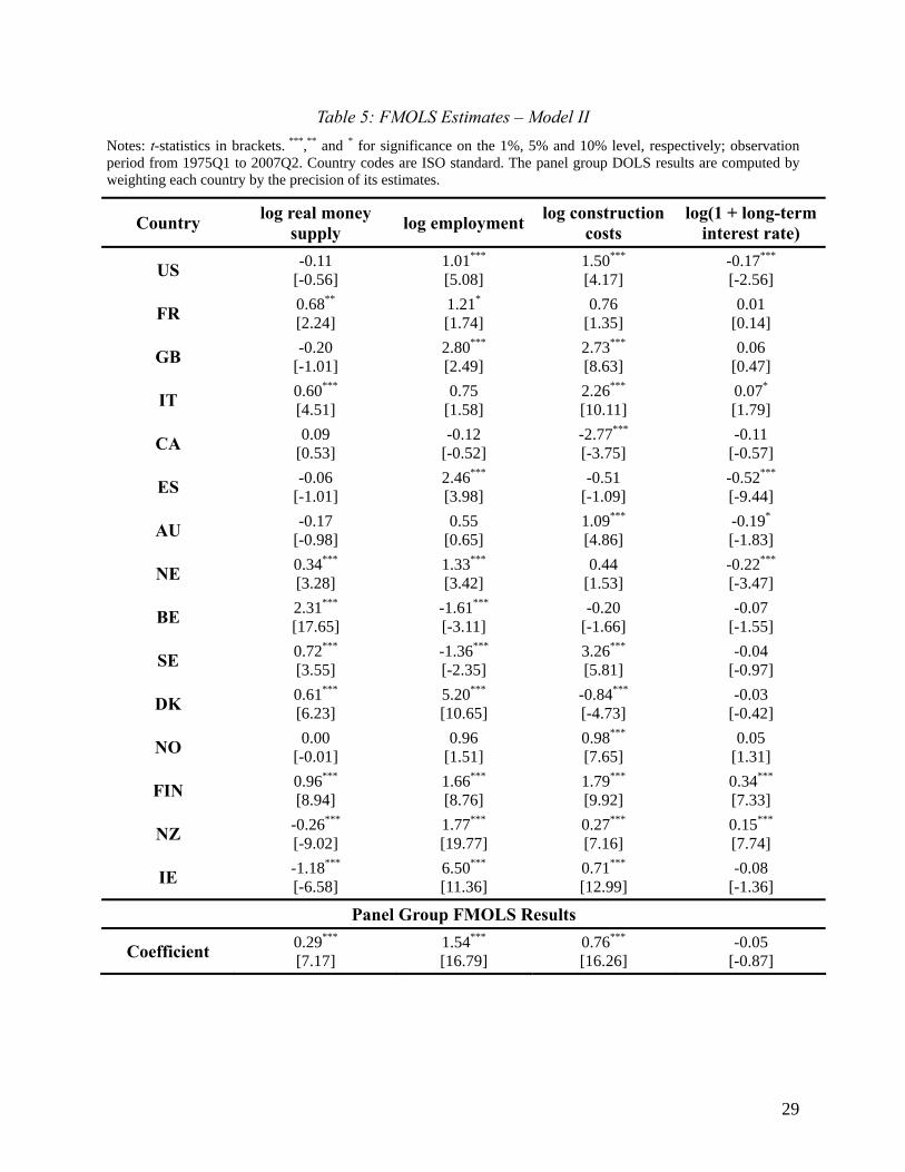
Table 5: FMOLS Estimates – Model II Notes: t-statistics in brackets. ***,** and * for significance on the 1%, 5% and 10% level, respectively; observation period from 1975Q1 to 2007Q2. Country codes are ISO standard. The panel group DOLS results are computed by weighting each country by the precision of its estimates.

Country log real money supply log employment log construction

costs log(1 + long-term

interest rate)

US -0.11 [-0.56]

1.01*** [5.08]

1.50*** [4.17]

-0.17*** [-2.56]

FR 0.68** [2.24]

1.21* [1.74]

0.76 [1.35]

0.01 [0.14]

GB -0.20 [-1.01]

2.80*** [2.49]

2.73*** [8.63]

0.06 [0.47]

IT 0.60*** [4.51]

0.75 [1.58]

2.26*** [10.11]

0.07* [1.79]

CA 0.09 [0.53]

-0.12 [-0.52]

-2.77*** [-3.75]

-0.11 [-0.57]

ES -0.06 [-1.01]

2.46*** [3.98]

-0.51 [-1.09]

-0.52*** [-9.44]

AU -0.17 [-0.98]

0.55 [0.65]

1.09*** [4.86]

-0.19* [-1.83]

NE 0.34*** [3.28]

1.33*** [3.42]

0.44 [1.53]

-0.22*** [-3.47]

BE 2.31*** [17.65]

-1.61*** [-3.11]

-0.20 [-1.66]

-0.07 [-1.55]

SE 0.72*** [3.55]

-1.36*** [-2.35]

3.26*** [5.81]

-0.04 [-0.97]

DK 0.61*** [6.23]

5.20*** [10.65]

-0.84*** [-4.73]

-0.03 [-0.42]

NO 0.00 [-0.01]

0.96 [1.51]

0.98*** [7.65]

0.05 [1.31]

FIN 0.96*** [8.94]

1.66*** [8.76]

1.79*** [9.92]

0.34*** [7.33]

NZ -0.26*** [-9.02]

1.77*** [19.77]

0.27*** [7.16]

0.15*** [7.74]

IE -1.18*** [-6.58]

6.50*** [11.36]

0.71*** [12.99]

-0.08 [-1.36]

Panel Group FMOLS Results

Coefficient 0.29*** [7.17]

1.54*** [16.79]

0.76*** [16.26]

-0.05 [-0.87]

29

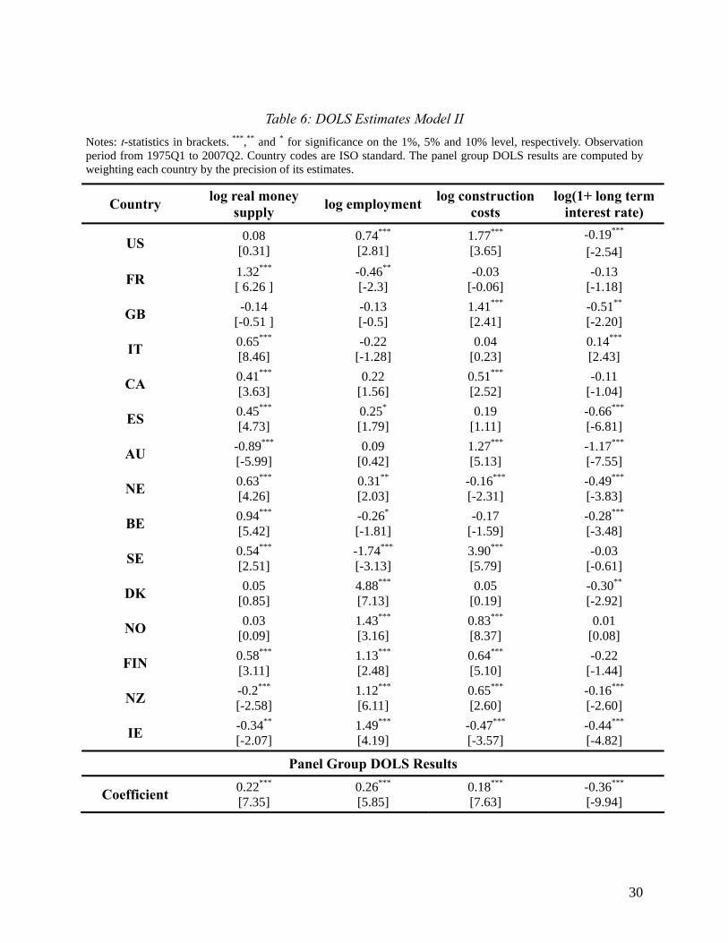
Table 6: DOLS Estimates Model II Notes: t-statistics in brackets. ***,** and * for significance on the 1%, 5% and 10% level, respectively. Observation period from 1975Q1 to 2007Q2. Country codes are ISO standard. The panel group DOLS results are computed by weighting each country by the precision of its estimates.

Country log real money supply log employment log construction

costs log(1+ long term

interest rate)

US 0.08 [0.31]

0.74*** [2.81]

1.77*** [3.65]

-0.19***

[-2.54]

FR 1.32*** [ 6.26 ]

-0.46** [-2.3]

-0.03 [-0.06]

-0.13 [-1.18]

GB -0.14 [-0.51 ]

-0.13 [-0.5]

1.41*** [2.41]

-0.51** [-2.20]

IT 0.65*** [8.46]

-0.22 [-1.28]

0.04 [0.23]

0.14*** [2.43]

CA 0.41*** [3.63]

0.22 [1.56]

0.51*** [2.52]

-0.11 [-1.04]

ES 0.45*** [4.73]

0.25* [1.79]

0.19 [1.11]

-0.66*** [-6.81]

AU -0.89*** [-5.99]

0.09 [0.42]

1.27*** [5.13]

-1.17*** [-7.55]

NE 0.63*** [4.26]

0.31** [2.03]

-0.16*** [-2.31]

-0.49*** [-3.83]

BE 0.94*** [5.42]

-0.26* [-1.81]

-0.17 [-1.59]

-0.28*** [-3.48]

SE 0.54*** [2.51]

-1.74*** [-3.13]

3.90*** [5.79]

-0.03 [-0.61]

DK 0.05 [0.85]

4.88*** [7.13]

0.05 [0.19]

-0.30** [-2.92]

NO 0.03 [0.09]

1.43*** [3.16]

0.83*** [8.37]

0.01 [0.08]

FIN 0.58*** [3.11]

1.13*** [2.48]

0.64*** [5.10]

-0.22 [-1.44]

NZ -0.2*** [-2.58]

1.12*** [6.11]

0.65*** [2.60]

-0.16*** [-2.60]

IE -0.34** [-2.07]

1.49*** [4.19]

-0.47*** [-3.57]

-0.44*** [-4.82]

Panel Group DOLS Results

Coefficient 0.22*** [7.35]

0.26*** [5.85]

0.18*** [7.63]

-0.36*** [-9.94]

30

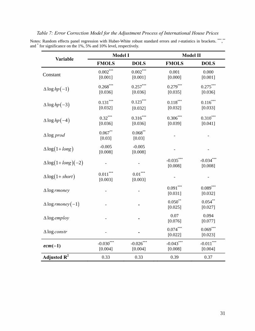
Table 7: Error Correction Model for the Adjustment Process of International House Prices Notes: Random effects panel regression with Huber-White robust standard errors and t-statistics in brackets. ***,** and * for significance on the 1%, 5% and 10% level, respectively.

Model I Model II Variable

FMOLS DOLS FMOLS DOLS

Constant 0.002*** [0.001]

0.002*** [0.001]

0.001 [0.000]

0.000 [0.001]

( )log 1hp∆ − 0.268*** [0.036]

0.257*** [0.036]

0.279*** [0.035]

0.275*** [0.036]

( )log 3hp∆ − 0.131*** [0.032]

0.123***

[0.032] 0.118***

[0.032] 0.116*** [0.033]

( )log 4hp∆ − 0.32*** [0.036]

0.316*** [0.036]

0.306*** [0.039]

0.310*** [0.041]

log prod∆ 0.067** [0.03]

0.068** [0.03]

- -

( )log 1 long∆ + -0.005 [0.008]

-0.005 [0.008]

- -

( )(log 1 2long∆ + − ) - - -0.035*** [0.008]

-0.034*** [0.008]

( )log 1 short∆ + 0.011*** [0.003]

0.01*** [0.003]

- -

log rmoney∆ - - 0.091*** [0.031]

0.089*** [0.032]

( )log 1rmoney∆ − - - 0.050** [0.025]

0.054** [0.027]

log employ∆ - - 0.07

[0.076] 0.094

[0.077]

log constr∆ - - 0.074*** [0.022]

0.069*** [0.023]

( 1)ecm − -0.030*** [0.004]

-0.026*** [0.004]

-0.043*** [0.008]

-0.011*** [0.004]

Adjusted R2 0.33 0.33 0.39 0.37

31