Macroeconomic Conditions and Capital Structure: Evidence

from Taiwan

Hsien-Hung Yeh and Eduardo Roca

No. 2010-14

ISSN 1836-8123

Series Editor: Dr. Alexandr Akimov

Copyright © 2010 by author(s). No part of this paper may be reproduced in any form, or stored in a retrieval system, without prior permission of the author(s).

1

Macroeconomic Conditions and Capital Structure: Evidence

from Taiwan

Hsien-Hung Yeh1

and Eduardo Roca2

1Department of Business Administration, National Pingtung University of Science and Technology,

Taiwan (Corresponding author)

2Department of Accounting, Finance and Economics, Griffith University, Nathan, Queensland 4111,

Australia

Abstract:

Using the partial adjustment model with the financial constraint of over-leverage and under-leverage

taken into account, this study investigates the impact of macroeconomic conditions and their

interactions with firm-specific factors on the determination of capital structure in the context of the

textile, plastics and electronics industries in Taiwan. The empirical results show that macroeconomic

conditions have a positive effect on capital structure decisions for firms with the financial constraint

of under-leverage relative to the target debt ratio. In addition, the interaction between

macroeconomic conditions and firm-specific variables also affects capital structure decisions;

however, this effect depends upon whether the firms are over-leveraged or under-leveraged relative

to their target debt ratios. Further, we also find the variation in the rate of adjustment toward their

target debt ratios that is dependent on whether the firms are over-leveraged or under-leveraged vis-

à-vis their debt-ratio target. This finding on adjustment rate is consistent with Byoun (2008) but does

not support Flannery and Rangan (2006).

Keywords: capital structure, macroeconomic conditions, financial constraint, partial adjustment

model.

1 Address for correspondence: Department of Business Administration, National Pingtung University of Science and Technology,

Nei-Pu, Pingtung 91207, Taiwan. Email: hhyeh@mail.npust.edu.tw, TEL: 886 8 7703202 Extension 7685, FAX: 886 8 7740367

2

1. Introduction

Over the last several decades, there has been a voluminous amount of studies on capital structure.

Focusing mainly on the effects of factors at the firm and industry levels, these studies have

documented common determinants of capital structure. Among these prior studies, some firm-

specific factors, namely firm size, growth opportunities, profitability, non-debt tax shields and asset

tangibility, affect the determination of capital structure. However, some of these firm-level

determinants of capital structure, for example growth opportunities, may vary with macroeconomic

conditions. In particular, there are more future investment and growth opportunities available at

economic trough than at economic peak. This suggests that firms would adjust their capital structure

in response to the change in growth opportunities arising from the fluctuations of macroeconomic

conditions, in particular at economic trough and peak. Thus, firms have to determine their capital

structure with macroeconomic conditions taken into account. However, based on different models of

capital structure, conflicting theoretical conclusions can be drawn on the impact of macroeconomic

conditions on capital structure, as discussed later in Literature Review. In spite of these, very few

studies have directly investigated the role of macroeconomic conditions in the determination of

capital structure. Thus, there is a need for further research on the effect of macroeconomic conditions

on capital structure.

Further, prior studies on capital structure have mostly been conducted based on developed countries

rather than on emerging economies. Glen and Singh (2004) find that capital structure in emerging

countries is different from that observed in developed countries. Taiwan has a successful experience

of economic transition from being an emerging country to becoming a developed one. The textile,

plastics and electronics industries played an important role in the economy of Taiwan during the

period from the 1960s to the mid-1990s. In addition, the textile, plastics and electronics industries

have labor-intensive, capital-intensive and technology-intensive characteristics, respectively.

Therefore, the study is conducted within the context of the textile, plastics and electronics industries

of Taiwan. In doing so, this study provides a new perspective on the impact of macroeconomic

conditions and their interactions with firm-specific variables on capital structure over the business

cycles.

This study utilizes the partial adjustment model of capital structure in examining the impact of

macroeconomic conditions on capital structure. In the application of the partial adjustment model,

financial constraint of over-leverage and under-leverage is not considered by prior studies. As

discussed later in the section of Methodology, the partial adjustment model permits us to neatly

investigate the effect of macroeconomic conditions on capital structure and to have a better

understanding of the adjustment behavior of capital structure decisions of firms with financial

constraint of over-leverage and under-leverage over the business cycles. This paper could provide

evidence of the following issues: (1) Does macroeconomic conditions affect the adjustment behavior

3

of capital structure? (2) Is capital structure influenced by the interactions between macroeconomic

conditions and firm-specific factors? and (3) Does the adjustment behavior of capital structure vary

with the financial constraint of over-leverage and under-leverage relative to the target capital

structure? The rest of the paper is organised as follows: Section 2 provides a literature review;

Section 3 discusses the methodology; the empirical results and analyses are presented in Section 4;

and finally, Section 5 concludes the study.

2. Literature Review

After the fundamental work of Modigliani and Miller (1958), extensive studies have been conducted

on capital structure decisions, as summarized by Harris and Raviv (1991). In addition, as stated

earlier, these previous studies have addressed the issue at the firm and industry levels and some

common determinants of capital structure at these levels have been identified. However, these

studies have rarely included macroeconomic conditions. Further literature review is discussed as

follows.

2.1 Macroeconomic Conditions and Capital Structure

Economic output and growth fall during the period of recession but increase during the period of

expansion, particularly at economic trough and peak. Some determinants of capital structure, for

example growth opportunities, may also vary with the current state of the economy over the business

cycles. There are more future growth opportunities at economic trough but less growth opportunities

at economic peak available to firms. The connection among macroeconomic conditions, firm-level

factors and capital structure suggests that capital structure will be related to macroeconomic

conditions.

Stulz (1990) analyzes the problem of managerial discretion and capital structure in his model and

contends that financing policy, by influencing the resources under management’s control, can reduce

the costs of overinvestment and underinvestment arising from the agency problem between

management and shareholders. Stulz argues that management always benefits from increasing

investment even when the firm invests in a negative net present value (NPV) project. Thus, when

cash flow is high, management will have the incentive to invest too much in negative NPV investment

opportunities, i.e. overinvestment. On the other hand, when cash flow is low, managers may not

have sufficient funds to invest in positive NPV projects, thus resulting in underinvestment. This is

because shareholders cannot believe management pronouncements that cash flows are insufficient

and may therefore not be willing to provide additional funding.

Consequently, Stulz argues that firms’ financial policy could reduce the agency cost of managerial

discretion. Issuing debt that forces management to pay out funds when cash flow is high can reduce

the overinvestment cost but it can exacerbate the underinvestment cost when cash flow decreases.

On the other hand, issuing equity that increases the resources under management’s control reduces

4

the underinvestment cost but it can worsen the overinvestment when cash flow increases. To reduce

the cost of overinvestment and underinvestment, firms finance with more debt when cash flow

increases but finance with less debt when cash flow decreases. Jensen’s free cash flow theory (1986)

also asserts that debt can be used to motivate managers and their organizations to be efficient in the

case of large free cash flow. Thus, firms would tradeoff the benefit of increasing leverage against the

cost of bankruptcy arising from the increase in debt to determine their optimal leverage. Stulz (1990)

concludes that optimal face value of debt increases if cash flow increases. This implies that, in order

to reduce the agency problem between management and shareholders, firms would finance with

more debt at economic peak due to the increase in cash flow but with less debt at economic trough

due to the decrease in cash flow. Therefore, capital structure will be positively related to

macroeconomic conditions.

However, the asymmetric information models arrive at opposite conclusion about the impact of free

cash flow and profitability on capital structure due to the asymmetric information problem between

management and outside investors. The asymmetric information models assume that investors are

less well informed than the inside management about the value of the firm’s assets. The information

asymmetry attributes to the under-pricing of firms’ equity and then firm’s underinvestment occurs.

Ross (1977) argues that firms tend to issue debt to be taken as a valid signal of a more productive

firm. In addition, Myers and Majluf (1984) argue that there is a pecking order of financing: firms will

finance new investment first with internal funds, then with debt, and finally with equity. Further,

Narayanan (1988), assuming that debt is risky rather than assumedly risk-free in the model of Myers

and Majluf (1984), analyzes this issue further in his model and concludes that debt is always better

than equity which is therefore consistent with the pecking order theory of financing. Narayanan also

contends that, in a world of asymmetric information regarding the new investment opportunity, firms

tend to finance with debt rather than its undervalued equity to avoid underinvestment. This implies

that, based on the asymmetric information theory, firms tend to finance with debt rather than equity

to avoid passing up valuable investment opportunities at economic trough. Therefore, capital

structure will be negatively correlated with macroeconomic conditions according to the asymmetric

information models.

Miller (1977) reported that debt ratios of the typical non-financial companies varied with the business

cycles between 1920 and 1960 and, in addition, debt ratios tended to fall during economic

expansions. Ferri and Jones (1979) examined the determinants of capital structure for the years

during expansion and recession, respectively. Their results suggest that capital structure seems to

vary with macroeconomic conditions. However, Ferri and Jones (1979) did not provide clear-cut

evidence on the impact of macroeconomic conditions on capital structure. Korajczyk and Levy (2003)

examine the impact of macroeconomic conditions on capital structure. They split their sample into

two sub-samples, financially constrained and financially unconstrained, which allows them to test

whether the tradeoff theory and the pecking order theory can explain the effects of financial

5

constraints and macroeconomic conditions on capital structure decisions. Korajczyk and Levy find

that corporate leverage is counter-cyclical for financially unconstrained firms. Hackbarth, Miao and

Morellec (2006) present a contingency-claims model and analyze credit risk and capital structure.

They argue that shareholders’ value-maximization default policy is characterized by a different

threshold for each state and, in addition, default thresholds are countercyclical. Their model predicts

that market leverage should be countercyclical. Further, Levy and Hennessy (2007) develop a general

equilibrium model for corporate financing over the business cycles. Levy and Hennessy argue that

managers would hold a proportion of their firm’s equity, i.e. managerial equity shares, in order to

avoid agency conflicts. Firms finance less debt due to the increases in managerial wealth and in risk

sharing during expansions than during contractions. Based on their simulations, Levy and Hennessy

find a counter-cyclical variation in leverage for less constrained firms. Their finding on a negative

effect of macroeconomic conditions on capital structure is consistent with Korajczyk and Levy (2003).

Based on the above discussion, it appears therefore that, theoretically, there is no agreement as to

the impact of macroeconomic conditions on capital structure. Thus, this paper addresses this gap for

further evidence from Taiwan, a newly industrialized country.

2.2 Interactions between Macroeconomic Conditions and Firm-Level Factors

As suggested by prior studies, capital structure is related to firm-specific variables such as growth

opportunities, profitability and the level of firm sales. In addition, as discussed earlier in the last

subsection, firm-specific variables such as growth opportunities and profitability vary with

macroeconomic conditions over the business cycles. These suggest that the relationship between

capital structure and its firm-level determinants is influenced by macroeconomic conditions.

However, rarely did previous studies address the impact of interactions between macroeconomic

conditions and firm-level factors on capital structure. As stated previously, Ferri and Jones (1979) find

that the relationship between firm size and capital structure is positive during economic expansion

but not significant during economic recession. Nonetheless, no studies provide evidence on the

impact of interactions between firm-level variables and macroeconomic conditions. Thus, this paper

addresses the issue to provide evidence of the interaction effect on capital structure decisions.

3. Methodology

This section discusses the econometric model for the adjustment behavior of capital structure first,

followed by the research sample and period and the operational definitions for the variables. Finally,

the empirical models for the capital structure adjustment and the actual level of capital structure of

firms with financial constraint of over-leverage and under-leverage relative to the target capital

structure over business cycles in the study is discussed.

3.1 Econometric Model of Capital Structure

6

As suggested by previous studies (Byoun 2008; Flannery & Rangan 2006; Hovakimian et al. 2001;

Marsh 1982; Taggart 1977), firms adjust toward the target capital structure over time. Following the

related studies, in particular Flannery and Rangan (2006) and Byoun (2008), this study utilizes the

model to examine the impact of macroeconomic conditions and their interactions with firm-specific

variables on the adjustment behavior of capital structure over the business cycles. The extent of the

capital structure adjustment or the change in capital structure from the previous level to the current

one can be expressed as a proportion (ρ) of the difference between the target capital structure ( *itY )

and the previous capital structure ( 1−itY ). In the application of the partial adjustment model, the

capital structure adjustment can be expressed as follows:

ititittitit YYYY ερ +−=− −− )( 1*

1 (1)

where, itY : the actual capital structure of firm i at the end of year t, 1−itY : the actual capital structure

of firm i at the beginning of year t, ρ: the adjustment speed or the proportion of the difference

between the target capital structure and the actual capital structure of previous year, Yit*: the target

capital structure of firm i at year t and itε : error term. It is worth noting that the rate of adjustment

toward the target level is between 0 and 1 according to most of the application of the partial

adjustment model.

The capital structure adjustment depends upon whether financial constraint of a positive or a

negative adjustment gap exists between the target capital structure and the previous capital

structure. Firms have the financial constraint of under-leverage relative to the target capital structure

if the gap between the target capital structure and the previous capital structure is positive. The

greater the adjustment speed, the greater is the increase in capital structure and the smaller is the

spare debt capacity that can be reserved for future investment and growth opportunities. On the

other hand, firms have the financial constraint of over-leverage relative to the target capital structure

if the gap between the target capital structure and the previous capital structure is negative. The

greater the adjustment speed, the greater is the decrease in capital structure and the smaller is the

probability that firms get into financial distress or go bankrupt. In brief, the relationship between the

adjustment rate and the capital structure adjustment varies according to whether the financial

constraint is over-leverage or under-leverage relative to the target capital structure. Therefore, this

paper takes the financial constraint of over-leverage and under-leverage into account in the

application of the partial adjustment model to investigate the impact of macroeconomic conditions

and the interactions of macroeconomic conditions and firm-specific factors on capital structure over

the business cycles.

However, the target capital structure is unobservable in the partial adjustment model. As suggested

by prior studies (Ferri & Jones 1979; Flannery & Rangan 2006; Harris & Raviv 1991; Hovakimian et al.

7

2001; Korajczyk & Levy 2003), we assume that the target capital structure is a linear function of firm-

specific variables, industry type, macroeconomic conditions and the interactions between firm-

specific variables and macroeconomic conditions. This study includes these variables in the partial

adjustment model through *itY to examine the significance of macroeconomic conditions and their

interactions with firm-specific variables in the determination of capital structure over business cycles.

The firm-specific factors, namely firm size, growth opportunities, profitability, non-debt tax shields

and asset tangibility, and industry type are used as control variables to capture the firm-specific and

industry effects in examining the impact of macroeconomic conditions and their interactions with

firm-specific variables on capital structure. Consequently, the equation for the target capital

structure )( *itY can be expressed as follows:

∑∑=

+=

×+++=k

jit

FCjitjtkit

ECtit

INDt

k

j

FCjitjtit ECXECINDXY

11

* ββββ (2)

where, Yit*: the target capital structure of firm i at the end of year t, β: regression coefficient, FC

jitX :

the firm-specific variable j at firm i at year t and j = 1 to k, IND: industry type, EC: macroeconomic

conditions and itFCjit ECX × : interactions between firm-specific variables and macroeconomic

conditions for firm i at year t. The former two items in the right side of Equation 2 are control

variables, namely firm-specific factors and industry type. The latter two items in the right side of

Equation 2 are test variables, namely macroeconomic conditions and their interactions with firm-

specific factors.

Substituting *itY in Equation 2 into Equation 1, we derive the equation for the determination of

capital structure adjustment )( 1−− itit YY as follows:

itit

c

jit

FCjit

ECFCjtit

ECtit

INDt

c

j

FCjitjttitit YECXECINDXYY εββββρ +−×+++=− −

=

×

=− ∑∑ )( 1

111 (3)

Incorporating the firm-specific variables, as suggested by prior studies, into Equation 3, we rewrite

the equation as follows:

itittitittititt

itittititt

ititttitEC

ttitIND

ttitt

ittittittitttitit

YECYTANGIBILITECNDTSECITYPROFITABILECGROWTH

ECSIZEECINDYTANGIBILITNDTSITYPROFITABILGROWTHSIZEYY

ερββββ

βρβρβρβ

ββββρ

+−×+×+×+×+

×++++

+++=−

−

−

1109

87

65

43211

)

()

(

(4)

where, itY : the actual capital structure of firm i at the end of year t, 1−itY : the actual capital structure

of firm i at the beginning of year t, ρ: the adjustment speed or the proportion of the gap of

8

( 1*

−− itit YY ), β: regression coefficient, SIZE: firm size, GROWTH: growth opportunities, PROFITABILITY:

profitability, NDTS: non-debt tax shields, TANGIBILITY: asset tangibility, EC: macroeconomic

conditions, SIZE×EC, GROWTH×EC, PROFITABILITY×EC, NDTS×EC and TANGIBILITY×EC: interactions

between firm-specific variables and macroeconomic conditions and ε: error term.

Rearranging Equation 4, then Equation 5 for the determination of the actual capital structure

)( itY can be obtained as written as follows:

itittitittititt

itittititt

ititttitEC

ttitIND

ttitt

ittittittitttit

YECYTANGIBILITECNDTSECITYPROFITABILECGROWTH

ECSIZEECINDYTANGIBILITNDTSITYPROFITABILGROWTHSIZEY

ερββββ

βρβρβρβ

ββββρ

+−+×+×+×+×+

×++++

+++=

−1109

87

65

4321

)1()

()

(

(5)

Equations 4 and 5 represent the econometric models used for the determination of capital structure

adjustment and actual capital structure for firms with financial constraints of over-leverage and

under-leverage taken into account to examine the significance of macroeconomic conditions and their

interactions with firm-specific variables in the determination of capital structure in this study.

Equations 4 and 5 reflect the adjustment behavior of capital structure of firms. Firms may deviate

away from their target capital structure over the business cycles when the adjustment rate is not

equal to 1. When the adjustment rate is equal to 1, then the actual capital structure is exactly same as

the target capital structure and no gap exists between them. In other words, the partial regression

coefficient of the precious actual capital structure will be significantly greater than 0 and different

from 1 whenever the deviation away from the target capital structure occurs.

3.2 Research Sample and Period

This study is conducted within the industries of textile, plastics and electronics that are labor-

intensive, capital-intensive and technology-intensive, respectively. The sample firms in these

industries are listed on the Taiwan Stock Exchange and have complete financial data in the research

period. However, we exclude the firms that experienced financial distress or trade suspension on the

Taiwan Stock Exchange.

The research period starts from 1983 and ends in 1995. The year 1983 is chosen as the starting point

for the study due to the reason of data availability, particularly in relation to the electronics industry

that started to take off only in the 1980s in Taiwan. The choice of 1995 as the end of the sample

period risks judgment of the study as being “dated”; doing so, however, allows the study to control

for and avoid a number of other intervening and complicating factors which occurred after 1995 such

as the Asian Financial Crisis in 1997 and the implementation of a tax integration in Taiwan on January

1, 1998. Thus, given these considerations, the sample period from 1983 to 1995 allows the study to

9

examine in a robust and reliable manner the impact of macroeconomic conditions on capital structure

decisions in the context of Taiwan over three business cycles.

Further, the research period covering three business cycles allows an examination on the effect of

macroeconomic conditions on capital structure decisions and a better understanding of the

adjustment behavior of capital structure decisions. The research is conducted at the years of

economic peak and trough during the period from 1983 to 1995. According to the reference dates

shown in the Business Indicators published by the Council for Economic Planning and Development of

Executive Yuan of Taiwan, the years at the economic peak and trough are used to represent the shifts

in macroeconomic conditions. Therefore, the years of 1983, 1988 and 1994 closest to the reference

dates of economic peak and the years of 1985, 1990 and 1995 closest to the reference dates of

economic trough, respectively, are selected to represent the shifts in macroeconomic conditions over

three business cycles.

3.3 Operational Definitions

The dependent variable of corporate capital structure and the explanatory variables at the firm level,

except the dummy variables, are calculated at book value. The operational definitions for the

dependent variable, the test variables including macroeconomic conditions and interactions between

macroeconomic conditions and firm-specific variables as well as the control variables are described as

follows:

Following most of prior empirical studies, the ratio of total debts to total assets, i.e. total debt ratio

(DR), and the change in the debt ratios (dDR) are used as a proxy for the dependent variable of the

actual capital structure and the capital structure adjustment, respectively. Further, we use binary

dummy variable (EC) as a proxy for macroeconomic conditions with a value of 0 for years at economic

trough and 1 for years at economic peak. In order to control for the effect of business cycle, the

dummy variables, BC7 and BC8, with a value of 1 are used to indicate Business Cycle 7 and 8,

respectively. The dummy variables, BC7 and BC8, with a value of 0 are used to indicate Business Cycle

6. Furthermore, we use the product of firm-specific variables and macroeconomic conditions as a

proxy for the interactions of macroeconomic conditions and firm-specific variables (Jaccard & Turrisi

2003).

As suggested by prior studies, this study include the firm-specific and industry variables as control

variables in the model to avoid model misspecification and to control for the firm-specific and

industry effects as well. The major firm-specific determinants of capital structure such as firm size,

growth opportunity, profitability, non-debt tax shields and asset tangibility are used to control for

firm-specific effects. We utilize the natural logarithm of net sales (lnS) as a proxy for firm size (Booth

2001; Chu et al. 1992; Huang & Song 2006; Rajan & Zingales 1995; Titman & Wessels 1988;

Wiwattanakantang 1999). The annual growth rate of total assets (gTA) is used as the proxy for

10

growth opportunity (Bevan & Danbolt 2002; Titman & Wessels 1988). The ratio of net operating

income to total assets (OITA) is used to represent profitability (Titman & Wessels 1988). We use the

ratio of depreciation to total assets (DEPTA) as a proxy for non-debt tax shields (Chu et al. 1992; Kim

& Sorensen 1986; Titman & Wessels 1988; Wald 1999; Wiwattanakantang 1999). The ratio of

inventory plus net fixed asset to total assets (INVFATA) is used as a proxy for asset tangibility (Chu et

al. 1992; Downs 1993; Titman & Wessels 1988; Wald 1999). Further, to control for industry effect, the

dummy variables, IND13 and IND14, with a value of 1 are used to indicate the plastics and textile

industries, respectively. The dummy variables, IND13 and IND14, with a value of 0 are used to indicate

the electronics industry.

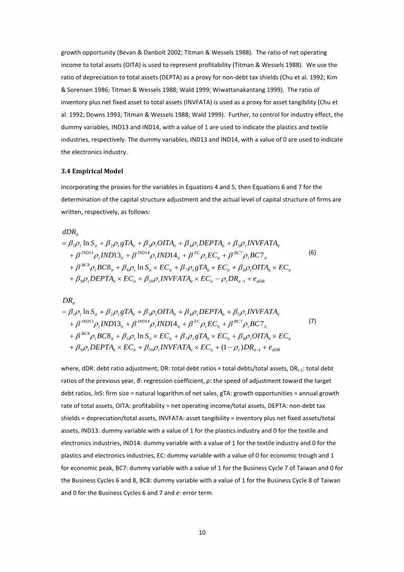
3.4 Empirical Model

Incorporating the proxies for the variables in Equations 4 and 5, then Equations 6 and 7 for the

determination of the capital structure adjustment and the actual level of capital structure of firms are

written, respectively, as follows:

dDRittitittititt

itittitittitittittBC

ittBC

ittEC

ittIND

ittIND

ittittittittitt

it

eDRECINVFATAECDEPTAECOITAECgTAECSBC

BCECINDINDINVFATADEPTAOITAgTAS

dDR

+−×+×+×+×+×++

++++

++++=

−1109

8768

7141354321

ln8

71413

ln

ρρβρβρβρβρβρβ

ρβρβρβρβ

ρβρβρβρβρβ (6)

dDRittitittititt

itittitittitittittBC

ittBC

ittEC

ittIND

ittIND

ittittittittitt

it

eDRECINVFATAECDEPTAECOITAECgTAECSBC

BCECINDINDINVFATADEPTAOITAgTAS

DR

+−+×+×+×+×+×++

++++

++++=

−1109

8768

7141354321

)1( ln8

71413

ln

ρρβρβρβρβρβρβ

ρβρβρβρβ

ρβρβρβρβρβ (7)

where, dDR: debt ratio adjustment; DR: total debt ratios = total debts/total assets, DRt-1: total debt

ratios of the previous year, β: regression coefficient, ρ: the speed of adjustment toward the target

debt ratios, lnS: firm size = natural logarithm of net sales, gTA: growth opportunities = annual growth

rate of total assets, OITA: profitability = net operating income/total assets, DEPTA: non-debt tax

shields = depreciation/total assets, INVFATA: asset tangibility = inventory plus net fixed assets/total

assets, IND13: dummy variable with a value of 1 for the plastics industry and 0 for the textile and

electronics industries, IND14: dummy variable with a value of 1 for the textile industry and 0 for the

plastics and electronics industries, EC: dummy variable with a value of 0 for economic trough and 1

for economic peak, BC7: dummy variable with a value of 1 for the Business Cycle 7 of Taiwan and 0 for

the Business Cycles 6 and 8, BC8: dummy variable with a value of 1 for the Business Cycle 8 of Taiwan

and 0 for the Business Cycles 6 and 7 and e: error term.

11

To investigate the adjustment behavior of capital structure of firms with financial constraints of over-

leverage and under-leverage taken into account over the selected business cycles according to

Equations 6 and 7, the study classifies the research sample into two subsamples based on negative

and positive adjustments: one subsample with a negative adjustment to represent the case of firms

with the financial constraint of over-leverage relative to the target debt ratio and another subsample

with a positive adjustment to represent the case of firms with the financial constraint of under-

leverage relative to the target debt ratio, as discussed earlier in Section 3.1. It is expected that, based

on the argument of Stulz (1990), macroeconomic conditions (EC) will have a positive effect on the

dependent variables (dDR and DR) in Equations 6 and 7. In addition, the regression coefficients of the

interactions between macroeconomic conditions and firm-specific variables will not be totally equal

to zero.

4. Empirical Results and Analyses

4.1 Data Analysis

The sample consists of the listed firms with the standard industrial classification (SIC) codes from 1301

to 1399, 1401 to 1499 and 2301 to 2399 in the textile, plastics and electronics industries of Taiwan.

The sample includes 627 observations of the listed firms in these industries during the years of

economic peak (i.e. 1983, 1988 and 1994) and trough (i.e. 1985, 1990 and 1995) over Business Cycles

6 to 8 in Taiwan. The debt ratios of the firms in the sample are less than 0.9. This suggests that no firm

in the sample is in financial distress. The descriptive statistics of the full sample are shown in Table 1.

In addition, no observations of ‘zero’ debt ratio adjustment are found in the sample. This shows that

the sample data allows the application of the partial adjustment model to investigate the adjustment

behavior of capital structure. Further, high correlation is found amongst the explanatory variables;

therefore, the centering technique suggested by Cronbach (1987) is utilized to avoid the problem of

multi-collinearity.

Table 1. Descriptive Statistics for the Full Sample

Variable

N

Mean

Standard Deviation

Minimum

Maximum

dDR 627 -0.02276 0.09831 -0.46459 0.32244 DRt 627 0.45062 0.17005 0.01396 0.87985 DRt-1 627 0.47338 0.17620 0.02426 0.89139 EC 627 0.46411 0.49911 0 1.00000 BC7 627 0.37321 0.48404 0 1.00000 BC8 627 0.50399 0.50038 0 1.00000 IND13 627 0.14514 0.35252 0 1.00000 IND14 627 0.38437 0.48683 0 1.00000 lnS 627 21.48528 1.20916 15.99580 25.23950 gTA 627 0.31132 0.47841 -0.30866 4.93033 OITA 627 0.08304 0.08064 -0.16390 0.59860 DEPTA 627 0.03618 0.02387 0 0.18216 INVFATA 627 0.55177 0.17214 0.02850 0.89525

Notes:

12

dDR = debt ratio adjustment; DRt = the debt ratio at time t; DRt-1 = the previous debt ratio at time t; EC = 0 for economic trough and 1 for economic peak; BC7 = 0 for Business Cycles 6 and 7, and 1 for Business Cycle 7; BC8 = 0 for Business Cycles 6 and 7, and 1 for Business Cycle 8; IND13 = 0 for the textile and electronics industries and 1 for the plastics industry; IND14 = 0 for the plastics and electronics industries and 1 for the textile industry; lnS = natural logarithm of net sales; gTA = annual growth rate of total assets; OITA = net operating income/total assets; DEPTA = depreciation/total assets; INVFATA = inventory plus net fixed assets/total assets.

4.2 Regression Results

Based on Equations 6 and 7, the regression results for the determination of the debt ratio adjustment

and the actual debt ratio in the subsamples with a negative and a positive adjustment gap are shown

in Tables 2 and 3, respectively. As shown in Note 4 of Table 2, the explanatory power, i.e. adjusted R-

square, of the models for the determination of the debt ratio adjustment and the actual debt ratio in

the subsample with a negative adjustment gap is 43.41% and 79.61%, respectively. In addition, no

serious residual auto-correlation problems are found according to the Durbin-Watson D value that is

close to 2, i.e. 1.957 as also shown in Note 4 of the table. Further, as can be seen in the VIF column of

Table 2, the values of variance inflation factor (VIF) much less than the critical value of 10 are often

regarded as indicating no problematic multi-collinearity (Chatterjee & Price 1991). Furthermore, no

sample observations with values of DFFITS are greater than 1.02 that indicates no outlier effect in the

subsample with a negative adjustment gap (Belsey et al. 1980).

Table 2. Regression Results in the Subsample with a Negative Adjustment Gap

Variables

(1) Dependent variable: Debt Ratio Adjustment (dDR)

(2) Dependent variable: Actual Debt Ratio (DR)

Coefficient

t Value

VIF5

Coefficient

t Value

VIF5

DRt-1 -0.14831 -5.81a 1.24180 0.85169 33.38a 1.24180 EC 0.01955 1.54 4.62215 0.01955 1.54 4.62215 BC7 -0.03833 -3.77a 2.75424 -0.03833 -3.77a 2.75424 BC8 -0.02832 -2.71a 3.25398 -0.02832 -2.71a 3.25398 IND13 0.00894 0.69 1.48972 0.00894 0.69 1.48972 IND14 -0.00279 -0.29 2.44645 -0.00279 -0.29 2.44645 lnS 0.00974 2.78a 1.14516 0.00974 2.78a 1.14516 gTA 0.00842 0.58 3.12928 0.00842 0.58 3.12928 OITA -0.18957 -2.65a 5.34009 -0.18957 -2.65a 5.34009 DEPTA -0.36932 -2.02b 4.36228 -0.36932 -2.02b 4.36228 INVFATA 0.06859 2.16b 1.88959 0.06859 2.16b 1.88959 lnS×EC -0.00474 -0.69b 1.09215 -0.00474 -0.69 1.09215 gTA×EC -0.06379 -2.69a 3.26808 -0.06379 -2.69a 3.26808 OITA×EC 0.12082 1.23 5.43026 0.12082 1.23 5.43026 DEPTA×EC -0.27691 -0.71 1.53247 -0.27691 -0.71 1.53247 INVFATA×EC 0.06152 1.06 1.58520 0.06152 1.06 1.58520

Notes: 1. dDRt = total debt ratio adjustment in the current year; DRt = total debt ratio at the end of the current year; DRt-1 = total debt ratio at the end of the previous year; EC = 0 for economic trough and 1 for economic peak; BC7 = 0 for Business Cycles 6 and 8 and 1 for Business Cycle 7; BC8 = 0 for Business Cycles 6 and 7 and 1 for Business Cycle 8;

13

IND13 = the dummy variable with a value of 1 for the plastics industry; IND14 = the dummy variable with a value of 1 for the textile industry; lnS = natural logarithm of net sales; gTA = annual growth rate of total assets; OITA = net operating income/total assets; DEPTA = depreciation/total assets; INVFATA = inventory plus net fixed assets/total assets; lnS×EC, gTA×EC, OITA×EC, DEPTA×EC and INVFATA×EC = interactions between firm-specific variables and macroeconomic conditions. 2. a, b and c indicate the significance level of 1%, 5% and 10%, respectively.

3. The value of the coefficient is the product of the rate of adjustment (ρ) and the regression coefficient (β) of each independent variable except the previous actual debt ratio (DRt-1) as shown in Equations 5-5 and 5-5A. 4. N Adj. R-square F value Durbin-Watson D value (1) 365 0.4341 18.56a 1.957 (2) 365 0.7961 90.05a 1.957 5. VIF: Variance Inflation Factor

Table 3. Regression Results in the Subsample with a Positive Adjustment Gap

Variables

(1) Dependent variable: Debt Ratio Adjustment (dDR)

(2) Dependent variable: Actual Debt Ratio (DR)

Coefficient

t Value

VIF5

Coefficient

t Value

VIF5

DRt-1 -0.03474 -1.63 1.52995 0.96526 45.39a 1.52995 EC 0.02614 2.79a 4.43960 0.02614 2.79a 4.43960 BC7 0.05854 6.30a 2.81518 0.05854 6.30a 2.81518 BC8 0.04836 5.61a 4.27679 0.04836 5.61a 4.27679 IND13 -0.00140 -0.14 1.55342 -0.00140 -0.14 1.55342 IND14 0.01052 1.37 2.16445 0.01052 1.37 2.16445 lnS -0.00284 -0.91 1.47421 -0.00284 -0.91 1.47421 gTA 0.05348 5.66a 4.23168 0.05348 5.66a 4.23168 OITA -0.09458 -1.42 4.33455 -0.09458 -1.42 4.33455 DEPTA 0.07070 0.45 4.31468 0.07070 0.45 4.31468 INVFATA 0.02752 1.11 1.91207 0.02752 1.11 1.91207 lnS×EC -0.00532 -0.90 1.32431 -0.00532 -0.90 1.32431 gTA×EC -0.03602 -2.80a 4.49244 -0.03602 -2.80a 4.49244 OITA×EC -0.01229 -0.13 4.43071 -0.01229 -0.13 4.43071 DEPTA×EC -0.49382 -1.43 1.52787 -0.49382 -1.43 1.52787 INVFATA×EC 0.10742 2.39b 1.58020 0.10742 2.39b 1.58020

Notes: 1. dDRt = total debt ratio adjustment in the current year; DRt = total debt ratio at the end of the current year; DRt-1 = total debt ratio at the end of the previous year; EC = 0 for economic trough and 1 for economic peak; BC7 = 0 for Business Cycles 6 and 8 and 1 for Business Cycle 7; BC8 = 0 for Business Cycles 6 and 7 and 1 for Business Cycle 8; IND13 = the dummy variable with a value of 1 for the plastics industry; IND14 = the dummy variable with a value of 1 for the textile industry; lnS = natural logarithm of net sales; gTA = annual growth rate of total assets; OITA = net operating income/total assets; DEPTA = depreciation/total assets; INVFATA = inventory plus net fixed assets/total assets; lnS×EC, gTA×EC, OITA×EC, DEPTA×EC and INVFATA×EC = interactions between firm-specific variables and macroeconomic conditions. 2. a, b and c indicate the significance level of 1%, 5% and 10%, respectively.

3. The value of the coefficient is the product of the rate of adjustment (ρ) and the regression coefficient (β) of each independent variable except the previous actual debt ratio (DRt-1) as shown in Equations 5-5 and 5-5A. 4. N Adj. R-square F value Durbin-Watson D value (1) 262 0.7210 43.32a 2.138 (2) 262 0.9161 179.75a 2.138 5. VIF: Variance Inflation Factor

14

On the other hand, the explanatory power, i.e. adjusted R-square, of the models for the

determination of the debt ratio adjustment and the actual debt ratio in the subsample with a positive

adjustment gap is 72.10% and 91.61%, respectively, as shown in Note 4 of Table 3. In addition, no

serious residual auto-correlation problems are found according to the value of Durbin-Watson D that

is close to 2, i.e. 2.138, as also shown in Note 4 of Table 3. Further, no serious multi-collinearity

problem is found according to the values of variance inflation factor (VIF) shown in the VIF column of

Table 3 that are much less than the critical value of 10. Furthermore, no sample observations with

values of DFFITS are greater than 1.02 that indicates no outlier effect in the subsample with a positive

adjustment gap (Belsey et al. 1980). Further analyses on the regression results in the subsamples with

a negative and a positive adjustment gap over Business Cycles 6 to 8 shown in Tables 2 and 3 are now

discussed.

4.2.1 Macroeconomic Conditions and Their Interactions with Firm-Specific Variables

According to the t-value shown in the t-value columns in Table 2 in the subsample with a negative

adjustment gap, the dummy proxy for macroeconomic conditions, i.e. EC, in the subsample with a

negative adjustment gap is not significantly related to the debt ratio adjustment and the actual debt

ratio of the listed firms in the textile, plastics and electronics industries during the period from 1983

to 1995 over Business Cycles 6 to 8 in Taiwan. On the other hand, according to the t-value shown in

Table 3 in the subsample with a positive adjustment gap, the dummy proxy for macroeconomic

conditions is statistically significant and positively related to the debt ratio adjustment and the actual

debt ratio of the listed firms in the textile, plastics and electronics industries over Business Cycles 6 to

8 in Taiwan. The result in the subsample with a positive adjustment gap is consistent with the

conclusion of Stulz (1990) that firms finance with less debt at economic trough in response to future

investment and growth opportunities. In addition, the findings in the subsamples with a negative or a

positive adjustment gap suggest that the effect of macroeconomic conditions on the debt ratio

adjustment and the debt ratios varies according to whether the adjustment gap between the target

debt ratio and the previous actual debt ratio is positive or negative.

Further, according to the t-value shown in the t-value columns in Table 2, the interaction between

growth opportunities and macroeconomic conditions (gTA×EC) is statistically significant and

negatively related to the debt ratio adjustment and the actual debt ratio in the subsample with a

negative adjustment gap. The results show that the effect of growth opportunities on the debt ratio

adjustment and the actual debt ratio is augmented by macroeconomic conditions although

macroeconomic conditions do not have a direct effect on the debt ratio adjustment and the actual

debt ratio in the subsample with a negative adjustment gap. On the other hand, according to the t-

value shown in Table 3, the interaction between growth opportunities and macroeconomic conditions

(gTA×EC) is statistically significant and negatively related to the debt ratio adjustment and the actual

debt ratio in the subsample with a positive adjustment gap. As can be seen in Table 3, growth

opportunities have a positive main effect on debt ratio but the effect is diminished by the negative

15

interaction with macroeconomic conditions. In addition, the interaction between asset tangibility and

macroeconomic conditions is statistically significant and positively related to the debt ratio

adjustment and the actual debt ratio in the subsample with a positive adjustment gap. The findings on

the interaction effect in the subsamples with negative and positive adjustment gaps illustrate the

variation in the effect of interactions between firm-specific variables and macroeconomic conditions

on the debt ratio adjustment and the actual debt ratio.

As a whole, the findings above suggest that the effects of macroeconomic conditions and their

interaction with firm-specific variables vary according to whether firms have the financial constraint

of over-leverage or under-leverage, i.e. a negative or a positive adjustment gap between the target

debt ratio and the previous actual debt ratio.

4.2.2 Adjustment Rate

Looking at the t-value shown in column t-value of Tables 2 and 3, regression coefficient of the

previous actual debt ratio (DRt-1) is significantly different from 0 in the case of a negative and a

positive gap over Business Cycles 6 to 8 for the listed firms in the textile, plastics and electronics

industries of Taiwan. The regression coefficient of the previous actual debt ratio in the empirical

model for the determination of actual debt ratio, i.e. Equation 7, is exactly equal to 1 minus the

adjustment rate of debt ratio adjustment (1−ρ). Therefore, the adjustment rate of debt ratio is

0.14831 (i.e. 1−0.85169) according to the regression coefficients of the previous actual debt ratio for

the determination of the debt ratio adjustment and the actual debt ratio in Table 2. On the other

hand, as shown in Table 3, the adjustment rate of debt ratio is 0.03474 (i.e. 1−0.96526) according to

the regression coefficient of the previous actual debt ratio for the determination of the debt ratio

adjustment and the actual debt ratio in the subsample with a positive adjustment gap. It is worth

noting that the effect of the explanatory variables, except the previous actual debt ratio, on the debt

ratio adjustment is a proportion of the regression coefficients of these variables in Equations 6 and 7.

The proportion depends upon the adjustment rate, as shown in Equations 6 and 7.

The findings above suggest that the adjustment rate of debt ratio for firms with a negative adjustment

gap, i.e. a financial constraint of over-leverage, is faster than for those with a positive adjustment gap,

i.e. a financial constraint of under-leverage. Firms with the financial constraint of over-leverage tend

to gear down their leverage due to the high risk of bankruptcy and adjust faster to rebalance their

debt ratio toward the target level. This suggests that firms adjust at a different rate of debt ratio

adjustment over time when they have a negative or a positive adjustment gap between the target

debt ratio and the previous actual debt ratio. This finding does not support the constant adjustment

rate of Flannery and Rangan (2006) but is consistent with Byoun (2008).

Moreover, in order to contrast the difference when negative and positive adjustment gaps are or are

not taken into account in the estimation of the modified partial adjustment model utilized in the

study, the regression results for the determination of the debt ratio adjustment and the actual debt

16

ratio in the full sample when negative and positive adjustment gaps are not taken into account are

shown in Table 4.

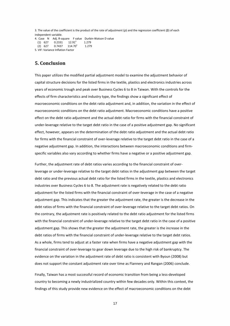
As shown in Note 4 in Table 4, the adjusted R-square for the model without negative and positive

adjustment gaps taken into account is much lower than that for the model used in the study, as

shown in Tables 2 and 3. There is residual auto-correlation problem due to the Durbin-Watson D

value (1.279) close to 1, as shown in Table 4. In addition, based on Equations 6 and 7, the regression

coefficient of the previous actual debt ratio is respectively equal exactly to the negative value of the

adjustment rate (−ρ) and to 1 minus the adjustment rate (1−ρ). The adjustment rate of debt ratio

(0.21824 or 1−0.78176) shown in Table 4 is overestimated without the adjustment gaps taken into

account. It is much higher than the adjustment rates of 0.14831 and 0.03474 shown respectively in

Tables 2 and 3 with negative and positive adjustment gaps taken into account. These additional

regression results reflect the fact that, in the application of the partial adjustment model for capital

structure adjustment, the estimation should take into account whether the adjustment gap between

the target capital structure and the previous actual capital structure is negative or positive.

Table 4. Regression Results in the Full Sample without Adjustment Gap Taken into Account

Variables

(1) Dependent variable: Debt Ratio Adjustment (dDR)

(2) Dependent variable: Actual Debt Ratio (DR)

Coefficient

t Value

VIF5

Coefficient

t Value

VIF5

DRt-1 -0.21824 -10.22a 1.19843 0.78176 36.60a 1.19843 IND13 0.03679 3.48a 4.38644 0.03679 3.48a 4.38644 IND14 -0.00448 -0.49 2.67337 -0.00448 -0.49 2.67337 EC -0.00201 -0.22 3.44276 -0.00201 -0.22 3.44276 BC7 0.00632 0.58 1.47378 0.00632 0.58 1.47378 BC8 -0.00321 -0.39 2.24711 -0.00321 -0.39 2.24711 lnS 0.00823 2.60a 1.23850 0.00823 2.60a 1.23850 gTA 0.05414 4.76a 3.56325 0.05414 4.76a 3.56325 OITA -0.29697 -4.61a 4.70518 -0.29697 -4.61a 4.70518 DEPTA -0.19678 -1.21 4.20475 -0.19678 -1.21 4.20475 INVFATA 0.08935 3.32a 1.81068 0.08935 3.32a 1.81068 lnS×EC -0.00921 -1.50 1.16342 -0.00921 -1.50 1.16342 gTA×EC -0.02852 -1.75c 3.66214 -0.02852 -1.75c 3.66214 OITA×EC 0.00751 0.08 4.76297 0.00751 0.08 4.76297 DEPTA×EC -0.55087 -1.58 1.48393 -0.55087 -1.58 1.48393 INVFATA×EC 0.12555 2.56b 1.50778 0.12555 2.56b 1.50778

Notes: 1. dDRt = total debt ratio adjustment in the current year; DRt = total debt ratio at the end of the current year; DRt-1 = total debt ratio at the end of the previous year; EC = 0 for economic trough and 1 for economic peak; BC7 = 0 for Business Cycles 6 and 8 and 1 for Business Cycle 7; BC8 = 0 for Business Cycles 6 and 7 and 1 for Business Cycle 8; IND13 = the dummy variable with a value of 1 for the plastics industry; IND14 = the dummy variable with a value of 1 for the textile industry; lnS = natural logarithm of net sales; gTA = annual growth rate of total assets; OITA = net operating income/total assets; DEPTA = depreciation/total assets; INVFATA = inventory plus net fixed assets/total assets; lnS×EC, gTA×EC, OITA×EC, DEPTA×EC and INVFATA×EC = interactions between firm-specific variables and macroeconomic conditions. 2. a, b and c indicate the significance level of 1%, 5% and 10%, respectively.

17

3. The value of the coefficient is the product of the rate of adjustment (ρ) and the regression coefficient (β) of each independent variable. 4. Case N Adj. R-square F value Durbin-Watson D value (1) 627 0.2331 12.91a 1.279 (2) 627 0.7437 114.70a 1.279 5. VIF: Variance Inflation Factor

5. Conclusion

This paper utilizes the modified partial adjustment model to examine the adjustment behavior of

capital structure decisions for the listed firms in the textile, plastics and electronics industries across

years of economic trough and peak over Business Cycles 6 to 8 in Taiwan. With the controls for the

effects of firm characteristics and industry type, the findings show a significant effect of

macroeconomic conditions on the debt ratio adjustment and, in addition, the variation in the effect of

macroeconomic conditions on the debt ratio adjustment. Macroeconomic conditions have a positive

effect on the debt ratio adjustment and the actual debt ratio for firms with the financial constraint of

under-leverage relative to the target debt ratio in the case of a positive adjustment gap. No significant

effect, however, appears on the determination of the debt ratio adjustment and the actual debt ratio

for firms with the financial constraint of over-leverage relative to the target debt ratio in the case of a

negative adjustment gap. In addition, the interactions between macroeconomic conditions and firm-

specific variables also vary according to whether firms have a negative or a positive adjustment gap.

Further, the adjustment rate of debt ratios varies according to the financial constraint of over-

leverage or under-leverage relative to the target debt ratios in the adjustment gap between the target

debt ratio and the previous actual debt ratio for the listed firms in the textile, plastics and electronics

industries over Business Cycles 6 to 8. The adjustment rate is negatively related to the debt ratio

adjustment for the listed firms with the financial constraint of over-leverage in the case of a negative

adjustment gap. This indicates that the greater the adjustment rate, the greater is the decrease in the

debt ratios of firms with the financial constraint of over-leverage relative to the target debt ratios. On

the contrary, the adjustment rate is positively related to the debt ratio adjustment for the listed firms

with the financial constraint of under-leverage relative to the target debt ratio in the case of a positive

adjustment gap. This shows that the greater the adjustment rate, the greater is the increase in the

debt ratios of firms with the financial constraint of under-leverage relative to the target debt ratios.

As a whole, firms tend to adjust at a faster rate when firms have a negative adjustment gap with the

financial constraint of over-leverage to gear down leverage due to the high risk of bankruptcy. The

evidence on the variation in the adjustment rate of debt ratio is consistent with Byoun (2008) but

does not support the constant adjustment rate over time as Flannery and Rangan (2006) conclude.

Finally, Taiwan has a most successful record of economic transition from being a less-developed

country to becoming a newly industrialized country within few decades only. Within this context, the

findings of this study provide new evidence on the effect of macroeconomic conditions on the debt

18

ratio adjustment and the determination of the actual debt ratios for firms with financial constraint of

over-leverage and under-leverage relative to the target debt ratios. Future research might address the

adjustment behaviour of capital structure decisions across the Asian countries to provide further

evidence on the effect of macroeconomic conditions and on the variation in the adjustment rate of

capital structure decisions. In particular, further evidence on the differences in the adjustment

behavior of capital structure between developing and developed countries leaves for future research.

Acknowledgements

An earlier version of the paper was presented at a refereed international scholarly conference hosted

by the Accounting and Finance Association of Australia and New Zealand held at the Gold Coast,

Queensland, Australia from July 1 to 3, 2007 and in the Queensland University of Technology – Griffith

University Finance Symposium organized by Professor of Finance, Michael Drew, and held at Griffith

University in November 2006. The authors are grateful for the helpful comments and suggestions

from the conference and symposium participants.

19

References

Belsey, D. A., Kuh, E., Welsch, R. E. (1980) Regression Diagnostics: Identifying Influential Data and

Sources of Collinearity. John Wiley and Sons, New York.

Bevan, A. A., Danbolt, J. (2002) Capital Structure and its Determinants in the UK: A Decompositional

Analysis. Applied Financial Economics, 12, pp. 159-70.

Booth, L., Aivazian, V., Demirguc-Kunt, A., Maksimovic, V. (2001) Capital Structures in Developing

Countries. Journal of Finance, 56, pp. 87-130.

Byoun, S. (2008) How and When Do Firms Adjust Their Capital Structures toward Targets? Journal of

Finance, 63, pp. 3069-96.

Chatterjee, S., Price, B. (1991) Regression Analysis by Example. John Wiley & Sons, New York.

Chu, P. Y., Wu, S., Chiou, S. F. (1992) The Determinants of Corporate Capital Structure Choice: Taiwan

Evidence. Journal of Management Science, 9, pp. 159-77.

Cronbach, L. (1987) Statistical Tests for Moderator Variables: Flaws in Analysis Recently Proposed.

Psychological Bulletin, 102, pp. 414-17.

Downs, T. W. (1993) Corporate Leverage and Nondebt Tax Shields: Evidence on Crowding-Out.

Financial Review, 28, pp. 549-83.

Ferri, M. G., Jones, W. H. (1979) Determinants of Financial Structure: A New Methodological

Approach. Journal of Finance, 34, pp. 631-44.

Flannery, M. J., Rangan, K. P. (2006) Partial Adjustment toward Target Capital Structures. Journal of

Financial Economics, 79, pp. 469-506.

Glen, J., Singh, A. (2004) Comparing Capital Structures and Rates of Return in Developed and

Emerging Markets. Emerging Markets Review, 5, pp. 161-92.

Hackbarth, D., Miao, J., Morellec, E. (2006) Capital Structure, Credit Risk, and Macroeconomic

Conditions. Journal of Financial Economics, 82, pp. 519-50.

Harris, M., Raviv, A. (1991) The Theory of Capital Structure. Journal of Finance, 46, pp. 297-355.

Hovakimian, A., Opler, T., Titman, S. (2001) The Debt-Equity Choice. Journal of Financial and

Quantitative Analysis, 36, pp. 1-24.

Huang, G., Song, F. M. (2006) The Determinants of Capital Structure: Evidence from China. China

Economic Review, 17, pp. 14-36.

20

Jaccard, J., Turrisi, R. (2003) Interaction Effects in Multiple Regression. Sage, Thousand Oaks.

Jensen, M. C. (1986) Agency Costs of Free Cash Flow, Corporate Finance, and Takeovers. American

Economic Review, 76, pp. 323-29.

Kim, W. S., Sorensen, E. H. (1986) Evidence on the Impact of the Agency Costs of Debt on Corporate

Debt Policy. Journal of Financial and Quantitative Analysis, 21, pp. 131-44.

Korajczyk, R. A., Levy, A. (2003) Capital Structure Choice: Macroeconomic Conditions and Financial

Constraints. Journal of Financial Economics, 68, pp. 75-109.

Levy, A., Hennessy, C. (2007) Why Does Capital Structure Choice Vary with Macroeconomic

Conditions? Journal of Monetary Economics, 54, pp. 1545-64.

Marsh, P. (1982) The Choice Between Equity and Debt: An Empirical Study. Journal of Finance, 37, pp.

121-44.

Miller, M. H. (1977) Debt and Taxes. Journal of Finance, 32, pp. 261-75.

Modigliani, F., Miller, M. H. (1958) The Cost of Capital, Corporation Finance and the Theory of

Investment. American Economic Review, 48, pp. 261-97.

Myers, S. C., Majluf, N. S. (1984) Corporate Financing and Investment Decisions When Firms Have

Information That Investors Do Not Have. Journal of Financial Economics, 13, pp. 187-221.

Narayanan, M. P. (1988) Debt versus Equity under Asymmetric Information. Journal of Financial and

Quantitative Analysis, 23, pp. 39-51.

Rajan, R. G., Zingales, L. (1995) What Do We Know about Capital Structure? Some Evidence from

International Data. Journal of Finance, 50, pp. 1421-60.

Ross, S. A. (1977) The Determination of Financial Structure: The Incentive-Signalling Approach. The

Bell Journal of Economics, 8, pp. 23-40.

Stulz, R. M. (1990) Managerial Discretion and Optimal Financing Policies. Journal of Financial

Economics, 26, pp. 3-27.

Taggart, R. A., Jr. (1977) A Model of Corporate Financing Decisions. Journal of Finance, 32, pp. 1467-

84.

Titman, S., Wessels, R. (1988) The Determinants of Capital Structure Choice. Journal of Finance, 43,

pp. 1-19.

Wald, J. K. (1999) How Firm Characteristics Affect Capital Structure: An International Comparison.

Journal of Financial Research, 22, pp. 161-87.

21

Wiwattanakantang, Y. (1999) An Empirical Study on the Determinants of the Capital Structure of Thai

Firms. Pacific-Basin Finance Journal, 7, pp. 371-403.