The views expressed in the article are those of the authors and do not necessarily represent the views of the Office of the Comptroller of the Currency, or the U.S. Department of Treasury, or the International Monetary Fund. The authors are responsible for all errors

Macroeconomic Changes as Drivers of Asset and Portfolio Performance

Alexander P. Attié

International Monetary Fund

Zheng-Feng Guo

Office of the Comptroller of the Currency

Zhenchang Xie

International Monetary Fund

January 2014

Abstract

In this paper, we first inverstigate the nonlinear relationship between asset class performance and forecasted macroeconomic factors, using a semiparametric multi-factor multivariate adaptive regression spline method(MARS). We then assess the varying impact of multipe macroeconomic factors, to which investors typically react, on asset performance. Finally, we propose an investment framework that the investors, both passive and active ones, can incorporate the dynamic relationship as a guide for strategic asset allocation decisions across different economic scenerios.

JEL Classification: C14, G11, G12

Keywords: Asset Returns, Macroeconomic Factors, Nonliearity, MARS, Portfolio Performance, Strategic Asset Allocation

Author’s E-Mail Address: aattie@imf.org, zhengfeng.guo@occ.treas.gov, zxie@imf.org

2

I. INTRODUCTION

Dynamics and changes in the business cycle and the resulting impact on capital markets are integral to the decision-making process of short and long-term investors, whether passive or active. Asset returns react to both financial and non-financial factors. For example, equity prices tend to increase to strong future corporate earnings (a financial factor) but also to future economic growth prospects (a macro-economic factor). From an investor’s perspective, the business cycle has always carried a critical importance, but the downturn of many economies in the wake of the global financial crisis, and the recovery since the trough of the crisis, have strengthened the importance of macroeconomic factors in the toolset of investors.

This paper investigates the dynamic relationship between asset returns and macroeconomic factors that are key drivers of the business cycle. These includes measures of growth (e.g. industrial production, business confidence indices, price indexes), unemployment, leading indicators, and the behavior of prices, which are an important causative factor in the cycle for the cost of labor per unit of output and levels of consumption. As such, these factors are exogenous to capital markets.

It is worth noting, however, that our analysis does not rely on the classic definition of the business cycle. Economic theory traditionally defines the business cycle as a fluctuation in aggregate economic activity that could be classified in one of four stages; expansion, crisis, recession, and recovery (Burns, 1980). From an investor’s point of view, fluctuations in the growth rate of the aggregate economy without a true recession could be sufficient to trigger a new set of investment behavior, or opportunity, therefore resulting in changes in asset prices. Hence, we prefer a definition of the business cycle that would not be too restrictive. For simplicity, it is assumed that a business cycle, or macroeconomic regime, is a period of time characterized by a set of distinct features falling within one of four categories: rising growth and inflation; rising growth and falling inflation; falling growth and rising inflation; and falling growth and falling inflation. Ignoring these regimes can expose an investor to periods of significant draw downs, even though an adequately diversified portfolio tends to recover in the long run. Conversely, recognizing them can offer opportunities to investors.

Our paper is closely related to the literature on nonlinear relationships between asset returns and macroeconomic factors. Early work in the literature includes Fama (1981), Geske and Roll (1983) and Asprem (1989), who explained the relationship between asset returns and one macroeconomic factor, inflation. In contrast, more recent literature has focused on multiple macroeconomic factors. For example, Schaller and Norden (1997) and Perez-Quiros and Timmermann (2000) implemented regime switching models to capture nonlinearity. McMillan (2001), Bredin and Hyde (2007) and Bradley and Jansen (2004) used the smooth transition autoregressive (STAR) model, which allows continuous regimes to capture the nonlinearity to model nonlinearity.

3

Our paper is also related to the vast literature on strategic asset allocation (SAA) with regime shifts. Ang and Bakaert (2002) investigated the dynamic asset allocation problem with regime-dependent correlations and volatilities in international equity markets. Vliet and Blitz (2009) identified four regimes in the economic cycles and proposed an investment approach for dynamic asset allocation across different economic regimes. Other works include Bredin, Hyde, and O’Reilly (2008), and Brière and Signori (2012).

Our work builds on a nonparametric method, a multi-factor multivariate adaptive regression spline (MARS) model, to identify the magnitude of change beyond which the impact on asset returns accelerates. This methodology is chosen because it offers more flexibility to model nonlinearity. Our work extends the work of Sheikh and Sun (2012), which used the same methodology, but differs from that in many important aspects. First, we attempt to overcome one of the shortcomings of many similar research pieces, namely the assumption of perfect foresight, so we rely on forecasted rather than realized macroeconomic factors to examine the relationship. We believe this is closer to the mindset of investors. Second, we show that incorporating the interaction terms in the MARS model is a critical improvement since the correlation between macro factors also contributes to explaining asset returns, which is another extension of their work. Finally, we examine the time-varying relationship between asset returns and macroeconomic factors and propose an investment strategy that can be easily implemented for both passive and active investors.

In this paper, a comprehensive quantitative process is applied to capture the complexity of the relationship between asset returns and a number of macroeconomic factors that are typically tracked by investors. We show that, like many others, the relationship between assets and forecasted macroeconomic factors are frequently non-linear, meaning that financial markets do not always react to changes in the economy in an orderly fashion. In light of the overabundance of information to which investors are confronted, we answer the following questions: (1) which factors matter most to investors? (2) How do they matter? (3) Do they always matter?

The simplicity and robustness of the MARS model offers a number of opportunities to investors. Key investment implications are illustrated through a tactical asset allocation model in which we show that re-optimizing a portfolio annually based on MARS signals helps improve total return and the Sharpe ratio of a portfolio. We embrace the idea that a selective approach within each broad asset class is necessary to best take advantage of macroeconomic signals, so we look at sub asset classes and equity styles and test results on U.S. Market.

The remainder of the paper is organized as follows. Section 2 presents our statistical methodology. Section 3 presents our data, followed by the empirical results in section 4. Section 5 applies our findings to investment decisions and concludes that changes in macroeconomic regimes provide a rationale for tactical tilts around a longer term strategic asset allocation. Section 6 concludes.

4

II. THE MODEL

Multivariate Adaptive Regression Splines (MARS) is a non-parametric regression procedure popularized by Friedman (1991). The MARS model offers the advantage of the flexibility of nonparametric models but without a curse of dimensionality. The MARS model can be viewed as a generalization of additive models and a recursive partitioning strategy.

The objective of the MARS model is to determine the relationship between a dependent variable y , e.g. asset returns, and one or more dependent variables x , e.g. macroeconomic

factors, where 1 2( , , )px x x x , given N observations of 1 2 1{ , , , }N

i i i pi iy x x x . The

relationship between y and x is described by

1 2( , , )p ty f x x x

Where t is the error term that captures the dependence of y other than 1 2( , , )px x x . t is

assumed to follow an i.i.d normal distribution with zero mean and unit variance. The goal is

to use the data to construct a function 1 2( , , )pf x x x to approximate the true functional form

1 2( , , )pf x x x.

Without further assumption on the functional form of f , the fully nonparametric

approximation of 1 2( , , )pf x x x to the true relationship 1 2( , , )pf x x x deteriorates, as the

dimension p increases, due to the curse of dimensionality issue. The additive model of Friedman and Silverman (1989) was introduced into the literature to circumvent this issue, which takes the form of

1

( ) .p

m m tm

y g x

Additive models are a very useful tool for approximating the multi-dimensional function

1 2( , , )pf x x x . The functions 1, pg g are univariate and can be estimated as well as the one-

dimensional nonparametric regression problems.

However, performance and computational consideration limit the number of variables that can be entered in additive models. Methods that approximate general functions in high dimensionality are proposed based on adaptive computation, which dynamically adjusts its strategy to take into account the function to be approximated. The MARS method applies the widely known recursive partition regression method with additive models. In other terms, the key idea is to split the entire region into several disjoint regions and use the simple additive model to approximate the functions in each sub region. The starting point is to approximate the function 1 2( , , )pf x x x in a set of basis functions

1

( ) ( ) .k

i i i ti

y f x I x R

5

where iR are disjoint sub regions representing a partition of the full domain D and ix is a

subset of x . The objective here is to use the data to simultaneously estimate a good set of sub region and the if s in each sub region.

To impose continuity at subregion boundaries, the continuity assumption is imposed on if s.

More specifically, the two-sided truncated power basis function of qth order is imposed, which is described as:

( )( )

( )

q

q q

t x if x tf x t

x t if x t

where q is the order of the spline and t is the knot location.

In the MARS, we specially restrict each function if to be a smooth function and we allow

the interaction terms between the basis functions. The MARS model can be written as

0( ) ( ) ( , ) ( , , )i i ij i j ijk i j kf x a f x f x x f x x x .

In the above equation, ( )i if x is the sum over all single variable basis functions involving

only ix . The second sum is a bivariate function that describes the interaction between two

variables. The third sum represents a sum over all three-variable basis functions. In this paper, however, we exclude the third sum because we only consider the interactions between our macro factors.

The central idea of the MARS model is to combine both the additive structure and modified regression partition to impose the continuity assumption. In terms of the partition of the sub regions, both forward searching and backward searching are implemented. To evaluate the model fitness, MARS uses the modified form of the generalized cross validation (GCV) first proposed by Craven and Wahba (1979). The GCV criterion of MARS can be written as

2

12

( )1

( )( )

1

N

i M ii

y f xGCV M

N C MN

Where M is the number of nonconstant basis functions and ( )C M is a complexity cost function, increasing with M, which accounts for increasing model complexity due to the inclusion of the basis functions. The GCV can be viewed as the average-squared residual of the fit to the data times a penalty to account for the increased variance associated with increasing model complexity(number of basis function M ).

III. THE DATA

This study uses data starting in the 1970s. The data are retrieved from the Global Financial Data, Barclays Capital, Datastream, and the Survey of Professional Forecasters, which

6

enables us to back test out the outcomes of our model against macroeconomic data forecasted as far back as in the 1970s.

For the U.S. market, we focus on traditional core assets, such as U.S. Treasuries, investment-grade corporate bonds, equities, a basket of commodities proxied by the Standard & Poor’s GSCI index, and marketable real estate investment trusts (REITs). We also look at different categories of bonds (agency mortgage-backed securities and high yield bonds), the 10 Global Industry Classification Standard (GICS) equity sectors, different equity styles (value and growth) and size. Whenever possible, we use indices that are actually tracked by investors. In some cases, we have stitched together different comparable indices to maximize the number of observations, provided that this does not introduce significant inconsistencies. For example, we use a 10-year government bond total return index sourced from Global Financial Data from 1970 until 1973, when the widely-used Barclays Capital U.S. Treasury index becomes available.

In this study, asset class returns data are year-over-year returns, sampled quarterly. The independent variables are year-over-year change of the macro factors, also sampled quarterly. In addition, we also standardize the change of the macro factors such that every data point is a degree measured in standard deviation from historical mean values.

Table 1 presents the descriptive statistics for the forecasted macroeconomic factors and asset returns. The hierarchy of returns is the following: U.S. government bond has the smallest return, followed by commodities, U. S. credit, growth stocks, value stocks, U.S. aggregate equities and small cap. Skewness and kurtosis are also different: negative skewness is pronounced for value stocks and growth stock, whereas REITs and U.S. credit exhibit high kurtosis.

IV. EMPIRICAL RESULTS

Our empirical results deliver a number of interesting messages. More specifically, we found that assets and macroeconomic factors exhibit a non-linear relationship, using forcasted macroeconomic factors; the importance of macroeconomic factors varies with time; finally, measuring the acceleration in the relationship is the key for tactical asset allocation decisions. We elaborate on these findings in the following subsections.

A. Result #1: evidence non-linearity

As is well documented in the literature, we find strong evidence of the non-linearity between most asset returns and forcasted changes in macroeconomic factors. In other terms, asset returns may overreact to changes in macroeconomic factors when the magnitude of this change, and sometimes its level, could herald the start of a new regime. In a first series of tests , we assess assets and factors’ properties jointly, using 4 main asset groups, U.S. treasuries, equities, REITs, and commodities, and 13 factors.1 However, rather than

1 These are: the international value of the dollar, the U.S. and world industrial production, the U.S. leading indicator index (LEI), the U.S. headline consumer price index (CPI) and personal consumption expenditures price index (PCE), the U.S. rate of unemployment, the Institute for Supply Management index (ISM), the level

(continued…)

7

presenting results for realized data, we opt for discussing the interaction with forecasted data instead. The reader may refer to Sheikh and Sun (2012) for empirical evidence on broad asset classes based on ex-post historical factors. In a second panel (Section B), we expand the number of assets to include different categories of bonds and equity sectors, style, and size, against these same factors. To compute results detailed below, we estimate MARS basis functions based on year-on-year changes in asset returns and levels of macroeconomic factors, with a quarterly frequency.

U.S. government bonds Figure 1 in the Appendix presents selected MARS basis functions and knots for U.S. government bonds. Results of MARS basis equations first reveal that the performance of U.S. government bonds (U.S. Treasuries) responds only to some factors while others matter perhaps less. For example, and somewhat surprisingly, U.S. Treasuries respond poorly to signals from U.S. corporate bond spreads and to changes in the level of mortgage delinquencies. This can be seen through the absence of a knot and the near-zero coefficient of MARS basis functions. These results do not suggest that such factors do not matter. Rather, they imply that the response is not systematic enough through time to define distinct regimes (i.e. no knot), and to identify an acceleration in the relationship (i.e. zero coefficient). For asset allocation decisions, this implies the signal is not material enough to be reliably used. Secondly, the relationship between U.S. Treasuries and our set of factors is, in most cases, asymmetrical. In other terms, the macroeconomic signal is stronger on one side of the knot than on the other. To illustrate this point, we find that returns of U.S. Treasuries rise when industrial production, but the response is less conclusive when industrial production rises. Findings are very similar with nominal GDP and a world industrial production index. Responses to changes in the leading indicator index are the mirror effect, with a non-zero and significant coefficient to the right of the knot. Focusing on inflation indicators, we find, along with previous studies discussed above, that bond returns are negatively affected by an increase in the rate of inflation, but we also conclude that U.S. Treasuries react negatively to falling prices if the magnitude of the drop exceeds a two-standard deviation move. The inverse relationship between nominal bonds and inflation is well documented: the real value of fixed nominal coupons diminishes over time; rising inflation triggers expectations of tighter monetary conditions which in turn push yields up and nominal bond prices down. The adverse reaction to rapidly falling prices, with possibly risks of deflation, is perhaps more surprising. In theory, deflation should make safe nominal government bonds more attractive, for instance to pension funds and investors seeking to match their long-term liabilities. But in fact, during the period under review, the U.S. economy never really experienced a sustained period of deflation. At most, the year-on-year CPI fell to -2.1 percent in 2009 and remained negative for 8 months, in the midst of the global financial crisis and unconventional stimulus measures implemented by the FOMC. While the latter boosted the returns of front-end maturities, longer-dated ones reacted

of the Federal Funds rate, U.S. corporate bond spreads, the level of U.S. housing starts, the level of U.S. mortgage delinquencies, and the U.S. nominal GDP index.

8

negatively.2 Investors started pricing in the risk that, ultimately, the unwinding of quantitative easing measures could push inflation higher. This risk is captured by the approximately 6-year duration index selected in this paper.

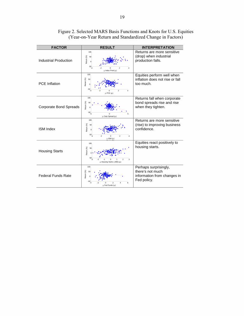
U.S. equities Figure 2 in the Appendix presents selected MARS basis functions and knots for U.S. equities. As in the case of U.S. Treasuries, results are asymmetrical in most cases; in some, such as changes in the Federal Funds rate, MARS basis functions yield relatively poor outcomes. Focusing first on growth factors, equity returns strongly react (negatively) to sharp downturns in lagging indicators, such as industrial production, whether domestic or global, and nominal GDP, but a rise in those factors is statistically less significant, as shown by the near-zero coefficient of MARS basis functions. Conversely, equities appear to be more responsive to an improvement, rather than a drop, in leading indicators. The same is true in the case of the housing market: a rise in housing starts triggers a stronger response than a drop, as it announces future improvements in construction, consumption, and corporate earnings; a drop in housing starts bears less significance; a sharp deterioration in the level of mortgage delinquencies is also an important driver of (negative) future performance, while an recovery in this factor appears to be less important. With respect to inflation indicators, we find that equities perform best when prices remain generally stable: a rise and a fall in prices both have a negative impact on equity returns. The strength of the signal is greater with the PCE index. Conventional finance theory holds that equities should provide an effective hedge against rising prices as they represent a claim on the dividend stream of real assets. In other words, at the aggregate level and in the long run, the corporate sector should pass on inflation in the form of higher prices, as noted by Mishkin (1992) and Boudoukh and Richardson (1993). In fact, however, empirical evidence shows that this is not the case: inflation shocks and periods of rising prices, as in the 1970s, tend to push equity prices down.3 In a similar fashion, rapidly falling prices also hurt equity returns, as they could lead to a deflationary regime and thus weigh on future corporate earnings.

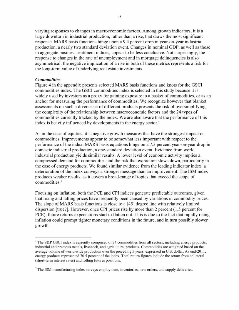
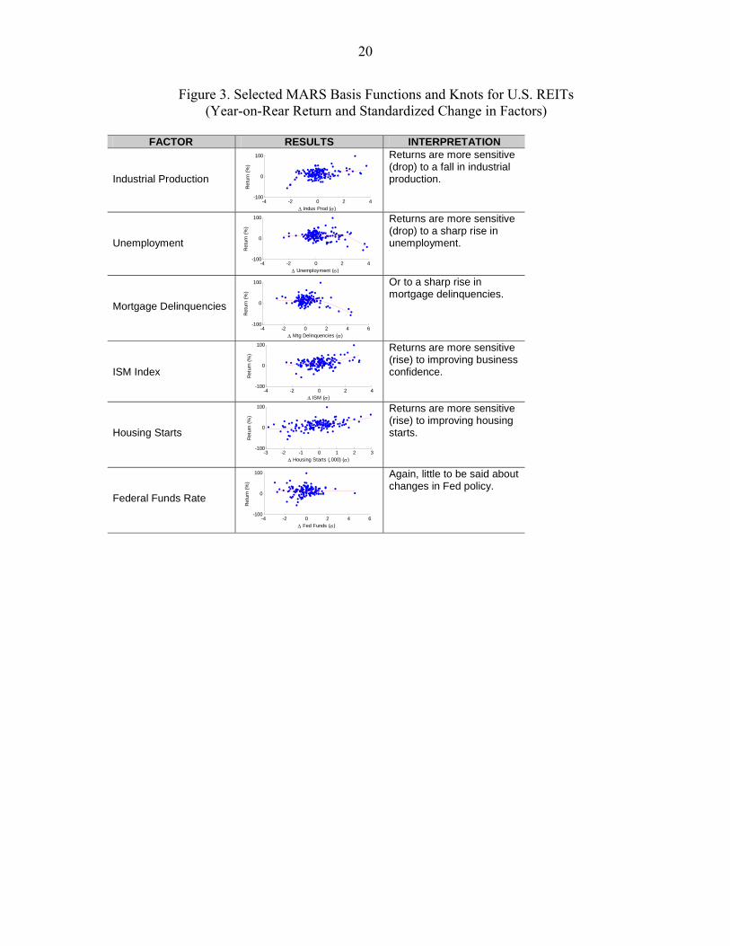
U.S. REITs Figure 3 in the appendix presents selected MARS basis functions and knots for U.S. REITS. Like the two preceding asset classes, REITs, a proxy for real estate investments, exhibit

2 From December 2008 to July 2009, the year-on-year headline CPI index fell from 0.1 percent to -2.1 percent, the lowest level since 1970. At the same time, the yield on the 30-year U.S. Treasury bond rose from 2.5 percent to about 4.5 percent, thus recording a sharp negative return. Shorter maturities, such as 2-year notes, remained little changed with yields at about 1 percent.

3 As noted by Bodie (1976), “this negative correlation [between equity prices and inflation] leads to the surprising and somewhat disturbing conclusion that to use common stocks as a hedge against inflation, one must sell them short”; see Bodie, Zvie, 1976, “Common Stocks as a Hedge Against Inflation,” Journal of Finance, Vol. 31, No. 2, pp. 459–470.

9

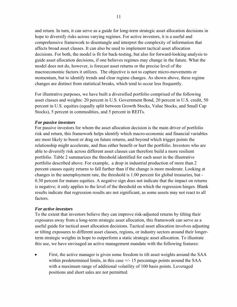
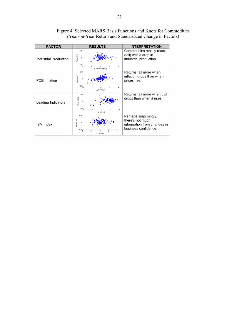
varying responses to changes in macroeconomic factors. Among growth indicators, it is a large downturn in industrial production, rather than a rise, that draws the most significant response. MARS basis functions hinge upon a 9.4 percent drop in year-on-year industrial production, a nearly two standard deviation event. Changes in nominal GDP, as well as those in aggregate business sentiment indices, appear to be less conclusive. Not surprisingly, the response to changes in the rate of unemployment and in mortgage delinquencies is also asymmetrical: the negative implication of a rise in both of these metrics represents a risk for the long-term value of underlying real estate investments. Commodities Figure 4 in the appendix presents selected MARS basis functions and knots for the GSCI commodities index. The GSCI commodities index is selected in this study because it is widely used by investors as a proxy for gaining exposure to a basket of commodities, or as an anchor for measuring the performance of commodities. We recognize however that blanket assessments on such a diverse set of different products presents the risk of oversimplifying the complexity of the relationship between macroeconomic factors and the 24 types of commodities currently tracked by the index. We are also aware that the performance of this index is heavily influenced by developments in the energy sector.4 As in the case of equities, it is negative growth measures that have the strongest impact on commodities. Improvements appear to be somewhat less important with respect to the performance of the index. MARS basis equations hinge on a 7.3 percent year-on-year drop in domestic industrial production, a one-standard deviation event. Evidence from world industrial production yields similar results. A lower level of economic activity implies a compressed demand for commodities and the risk that extraction slows down, particularly in the case of energy products. We found similar evidence from the leading indicator index: a deterioration of the index conveys a stronger message than an improvement. The ISM index produces weaker results, as it covers a broad-range of topics that exceed the scope of commodities.5

Focusing on inflation, both the PCE and CPI indices generate predictable outcomes, given that rising and falling prices have frequently been caused by variations in commodity prices. The slope of MARS basis functions is close to a [45] degree line with relatively limited dispersion [true?]. However, once CPI prices rise by more than 2 percent (1.5 percent for PCE), future returns expectations start to flatten out. This is due to the fact that rapidly rising inflation could prompt tighter monetary conditions in the future, and in turn possibly slower growth.

4 The S&P GSCI index is currently comprised of 24 commodities from all sectors, including energy products, industrial and precious metals, livestock, and agricultural products. Commodities are weighted based on the average volume of world-wide production over the preceding 5 years, expressed in U.S. dollar. As end-2011, energy products represented 70.5 percent of the index. Total return figures include the return from collateral (short-term interest rates) and rolling futures positions.

5 The ISM manufacturing index surveys employment, inventories, new orders, and supply deliveries.

10

B. Result # 2: which factors matter most and when: time-varying importance of factors

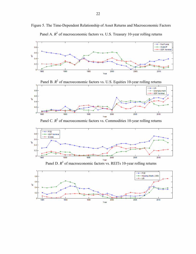
Results presented in the charts above are one-dimensional in order to provide a clear message to the reader, but in fact, historical evidence distilled through MARS basis functions estimated on past asset and factor data show that the relative importance of macroeconomic factors varies greatly with time and across different growth and inflation regimes. To estimate time dependent relationship, we measure explanatory attributes of macroeconomic factors on asset returns with a rolling window, where we use both rolling correlation and the square of the correlation coefficient between realized and modeled annual returns (R2) with a quarterly frequency with the window length being fixed for 10 years period. From an investor’s perspective, results have important practical implications. With abundant information available to investors, it is worth assessing which macroeconomic factors matter most, which of those matter perhaps less, and to what extent their relative explanatory power varies across different regimes. To explore the correlation dynamics between macroeconomic factors and asset returns, we study the time series properties of R-squared in the nonlinear regression of different asset returns on the macroeconomic factors we discussed above. It is noteworthy that in this subsection, we still focus on the one-to-one relationship. However, we plot the one-to-one relationship in one figure so we can show the correlation dynamics and the relative explanatory power of different factors across time. For simplicity and to better show our results, we will present the top three most important factors for the four asset groups, U.S. treasuries, equities, REITs, and commodities. We follow a moving window approach with a fixed window length of 10 years. First, we calculate the R-squared using the quarterly data from 1976 to 1985. Next, we move the window forward by one year, and we calculate the R-squared for the period 1977 through 1986. We use this 10-year moving window procedure to construct the time series of R-squared across three key macroeconomic factors. Figure 5 in the Appendix shows the dynamic correlation between and U. S. government bond and the three key macroeconomic factors. The top three most important factors for government bond are the Fed funds, industrial production and GDP growth. Not surprisingly, the correlation changes over time. For example, in the first regression, the R-squared of U.S. government bond versus Fed Funds is 0.66. In contrast, the R-squared in the last regression is 0.39. The correlation changes over time depending on different economic scenario. Most importantly, the figure shows the relative explanatory power of macroeconomic factors across time. We can observe similar time dependent properties for U.S. equities, commodities and REITS, see Panel B, Panel C and Panel D in Figure 5.

V. INVESTMENT IMPLICATIONS

The nonparametric nature of the MARS framework offers a lot of flexibility for investors, whether they are active or passive. For passive investors tracking one or several benchmark indices, it offers a systematic structure to understand which macroeconomic factors drive risk

11

and return. In turn, it can serve as a guide for long-term strategic asset allocation decisions in hope to diversify risks across varying regimes. For active investors, it is a useful and comprehensive framework to disentangle and interpret the complexity of information that affects broad asset classes. It can also be used to implement tactical asset allocation decisions. For both, the model is fit for back-testing, but also for forward-looking analysis to guide asset allocation decisions, if one believes regimes may change in the future. What the model does not do, however, is forecast asset returns or the precise level of the macroeconomic factors it utilizes. The objective is not to capture micro-movements or momentum, but to identify trends and clear regime changes. As shown above, these regime changes are distinct from statistical breaks, which tend to occur less frequently.

For illustrative purposes, we have built a diversified portfolio comprised of the following asset classes and weights: 20 percent in U.S. Government Bond, 20 percent in U.S. credit, 50 percent in U.S. equities (equally split between Growth Stocks, Value Stocks, and Small Cap Stocks), 5 percent in commodities, and 5 percent in REITs.

For passive investors For passive investors for whom the asset allocation decision is the main driver of portfolio risk and return, this framework helps identify which macro-economic and financial variables are most likely to boost or drag on future returns, and beyond which trigger points the relationship might accelerate, and thus either benefit or hurt the portfolio. Investors who are able to diversify risk across different asset classes can therefore build a more resilient portfolio. Table 2 summarizes the threshold identified for each asset in the illustrative portfolio described above. For example, a drop in industrial production of more than 2 percent causes equity returns to fall further than if the change is more moderate. Looking at changes in the unemployment rate, the threshold is 1.00 percent for global treasuries, but -0.30 percent for mature equities. A negative sign does not indicate that the impact on returns is negative; it only applies to the level of the threshold on which the regression hinges. Blank results indicate that regression results are not significant, as some assets may not react to all factors.

For active investors To the extent that investors believe they can improve risk-adjusted returns by tilting their exposures away from a long-term strategic asset allocation, this framework can serve as a useful guide for tactical asset allocation decisions. Tactical asset allocation involves adjusting or tilting exposures to different asset classes, regions, or industry sectors around their longer-term strategic weights in hope to outperform a static strategic asset allocation. To illustrate this use, we have envisaged an active management mandate with the following features:

First, the active manager is given some freedom to tilt asset weights around the SAA within predetermined limits, in this case +/- 15 percentage points around the SAA with a maximum range of additional volatility of 100 basis points. Leveraged positions and short sales are not permitted.

12

Second, the mandate encourages avoiding high frequency trading, meaning that the strategy aims at benefiting from meaningful regime changes rather than short-term momentum trends. This implies that tactical portfolio reallocations could occur rather infrequently, perhaps quarterly or annually.

Third, the intent of the tactical tilt is to improve the risk-adjusted return of the portfolio.

The algorithm for tactical asset allocation is relatively conventional, and in line with the approach used by Sheikh and Sun (2012). Where we differ however is with respect to the inputs. While MARS equations have a superior fit if historical (realized) data are employed, we find it useful to base our analysis on forecasted macroeconomic factors rather than realized ones, in order to remain close to the mindset of actual investors. As perfect foresight is an unrealistic assumption in real life, our framework requires a set of simple beliefs: based on current levels of macroeconomic factors, and one-year forward-looking expectations of these factors sourced from the Federal Reserve Bank of Philadelphia’s Survey of Professional Forecasters, investors only need to forecast the future direction of these variables rather than their exact level. For example, will inflation increase or decrease over the next 12 months? The OECD or the IMF World Economic Outlook (WEO) projections could also serve as useful inputs.

Turning to the algorithm, first we rank asset classes based on their ability to perform well against various expected changes in macro factors, using MARS equations with interaction terms. This is done by using the R2 of MARS equations. We have used other variables to rank the responses, including OLS and correlation, but found that the R2 works best in most cases. The ranking serves as a guide to over or underweight the portfolio versus the static SAA. Starting with the initial portfolio allocation, we re-optimize the portfolio holdings using a generic constrained optimization framework with the following constraints: exposure can fluctuate with +/- 15 percentage points around the target asset class allocation; there can be long-only positions with no leverage; the tracking error active risk budget envelope is set at 100 basis points; tilts aim at maximizing returns. We re-optimize the portfolio at various frequencies, quarterly, semi-annually, and annually, to evaluate optimal portfolio reweighting frequencies. The shape of the hinged relationship between assets and factors shown above provides an insight of how an active manager might interpret these linkages. Looking for instance at the relationship between U.S. equities and industrial production (see Figure 6 in the Appendix), the relationship is similar to the payoff of a covered call option strategy, where a call is sold on equities and the portfolio manager anticipates either stable or higher prices. In the case of corporate bonds and inflation (see Figure 6 in the Appendix), the relationship takes the form of a triangle: taking a position on corporate bond pays off if inflation remains within a range, akin a short straddle where a call and a put are sold. The association with options terminology was usefully made by Sheikh and Sun (2012) and is common in the investment industry, so we find it valuable to convey it here as well.

13

Could a regime-change inspired strategy add value vs. a static SAA? One way to answer the question is to back-test historical data to identify how an active manager might have reallocated the portfolio. Back-testing follows the following rules and assumptions:

The model for measuring the impact of factor changes on asset returns is defined once and for all at the beginning of the period. The period covered is 1986-present due to limited data for some assets. More recent information is progressively integrated by the model.

The model assesses asset returns and driving factors once a year. This frequency is chosen arbitrarily, but has the advantage of capturing meaningful regime shifts rather than short-lived trends. This infrequent readjustment risks missing the start of a new regime but, with this data sample, results are superior to a semi-annual or quarterly frequency.

The portfolio is optimized along the lines outlined above.

Tactical deviations, with limits for each asset class and constraints on overall risk tolerance, occur concurrently with signals provided by the model. Positions are kept for one year.

With no doubt, back-tested results of this hypothetical dynamic portfolio are higher than they would be in practice. We assumed that new positions are taken at the time factors express a significant change. In practice, some delay may occur. Manager may doubt signals and decide to wait and see. Moreover, transaction costs are excluded, while they could be material in some asset classes such as emerging markets, REITs, and corporate bonds. Nevertheless, the common sense underpinning the strategy is appealing to investors and explains, in part, the popularity of regime-aware investment strategies in the asset management industry. 6 This strategy is best thought, however, as a way to improve the risk-return features of a static SAA, not as an asset allocation tool or an absolute return strategy.

6 Regime-aware investment strategies are popular in the asset management industry. The framework used in this note is inspired from models and strategies employed in a number of firms: JP Morgan (A. Sheikh and J. Sun, 2011, Regime Change, JP Morgan Asset Management), Goldman Sachs (A. Timcenko and N. Weisberger, 2012, Acceleration Matters: Asset returns and the Business Cycle, Goldman Sachs ECS Research), State Street (F. Dodard, C. Goolgasian, J. Lépine, and S. Tadesse, 2011, A Case for Regime-Aware Dynamic Investment Process), Morgan Stanley (G. Peters et al., 2012, Correlation Regime Change, MS Cross Asset Strategy), Citi (K. Miller et al., 2011, Rising Influence of Macro-Economic Factors), Natixis (P. Artus, 2011, Asset Allocation, Inflation, and Macroeconomic Regimes, Natixis Corporate Banking), Deutsche Bank (S. Mesomeris et al., 2011, Style Performance in Different Macro Regimes), Robeco (P. Vliet and D. Blitz, 2009, Dynamic Strategic Asset Allocation: Risk and Return across Economic Regimes, Robeco Asset Management), and also Wellington, Blackrock, and a number of academic articles.

14

VI. CONCLUSION

In this paper, we provide a comprehensive framework to evaluate on the nonlinear relationship between asset returns and macroeconomic factors. We show that the impact of macroeconomic factors on asset returns and asset returns themselves are better forecasted when the relationship between macroeconomic factors is included (MARS with interaction terms). We finally propose an investment framework that the investors, can incorporate the dynamic relationship as a guide for strategic asset allocation decisions across different economic scenarios.

15

REFERENCES Ang, A. and G. Bekart, 2002, “International Asset Allocation with Regime Shift,” Review of Financial Studies, 15, pp. 1137-1187. Asprem, M. 1989, “Stock Prices, Asset Portfolio and Macroeconomic Variables in Ten European Countries,” Journal of Banking and Finance, 13, pp. 589-612. Biere, M. and O. Signori, 2012, “Inflation-Hedging Portfolios: Economic Regimes Matter,” Forthcoming in Journal of Portfolio Management. Blitz, D. and P. V. Vliet, 2009, “Dynamic Strategic Asset Allocation: Risk and Return across Economic Regimes”, Working paper. Bradley, M.D. and D.W. Jansen, 2004, “Forecasting with a Nonlinear Dynamic Model of Stock Returns and Industrial Production,” International Journal of Forecasting, Vol. 20, pp.321-342. Bredin, D. and S. Hyde, 2007, “ Regime Change and the Role of International Markets on the Stock Returns of Small Open Economies,” European Financial Management, Vol. 14, Issue 2, pp.315-346. Bredin, D., S. Hyde and G. O’Reilly, 2008, “Regime Changes in the Relationship between Stock Returns and the Macroeconomy”, working paper. Bodie, Z., 1976, “Common Stocks as a Hedge against Inflation,” Journal of Finance, Vol. 31, No. 2, pp. 459–470.

Boudoukh, J. and Richardson, M., 1993, “Stock Returns and Inflation: A Long-Horizon Perspective,” The American Economic Review, Vol.83, No.5, pp. 1346-1355. Burns, A .F. , 1980, “Measuring business cycles”, New York, National Bureau of Economic Research. Fama, E.,1981, “Stock Returns, Real Activity, Inflation, and Money,” The American Economic Review, Vol.71, 1981, pp.545-65. Friedman, J. H., 1991, “Multivariate Adaptive Regression Splines,” The Annal of Statistics, Vol.19, No.1, pp.1-503.

Friedman, J. H. and B. W. Silverman, 1989, “Flexible Parsimonious Smoothing and Additive Modeling,”Technometrics, Vol. 31, No. 1., pp. 3-21. Geske, R. and R. Roll, 1983 , “The Fiscal and Monetary Linkage Between Stock Returns and Inflation,” The Journal of Finance, Vol. 38, No.1, pp.1-33.

16

Guidolin, M. and A. Timmermann, 2008, “International Asset Allocation under Regime Switching, Skew, and Kurtosis Preferences,” The Review for Financial Studies, Vol. 21, No.2, pp.889-935. McMillan, D.G. 2001, “Nonlinear Predictability of Stock Market Returns: Evidence from Nonparametric and Threshold Models,” Journal of International Money and Finance, Vol. 4, pp.267-268. Mishkin, F. S., 1992, “Is the Fisher Effect for Real?” Journal of Monetary Economics, Vol. 30, No. 2, pp. 195–215. Perez-Quiros, G. and A. Timmermann, 2000, “Firm Size and Cyclical Variations in Stock Returns,” The Journal of Finance, Vol. 55, pp.1229-1292. Schaller, H. and S.V., Norden, 1997, "Regime Switching in Stock Market Returns," Applied Financial Economics, vol. 7(2), pp. 177-191. Sharpe, W.F, 1992, “Asset Allocation: Management Style and Performance Measurement,” The Journal of Portfolio Management, Winter 1992, pp.7-19. Sheikh, A.Z. and J. Sun, 2012, “Regime Change: Implications of Macroeconomic Shifts on Asset Class and Portfolio Performance,” The Journal of Investing, Vol. 21, No. 3, pp. 36-54.

17

Appendix

Table 1.Summary Statistics for Annual Returns

 U.S. Government bond 

US Credit  US Equities Growth Stocks 

Value Stocks 

Small Cap 

mean  8.2%  10.0% 12.5%  12.3% 12.8%  13.8%median  7.3%  8.7% 13.6%  12.3% 14.5%  14.7%min  ‐4.1%  ‐17.1% ‐38.0%  ‐41.2% ‐41.1%  ‐37.5%max  30.5%  46.1% 59.4%  62.5% 55.7%  97.5%skewness  0.92  1.00 ‐0.36  ‐0.31 ‐0.42  0.47kurtosis  4.40  5.22 3.18  3.02 3.50  4.17

Table 2. Summary of Thresholds and Robustness of the Results (R2) (YoY change in σ)

Note: units correspond to the way each factor is published. Headline PCE takes the form of a YoY percentage, so the hinge should be read as -1.56 percent for global treasuries, and -1.24 percent for linkers. In the case of IP, the hinge varies between -7 percent and -2 percent (yoy), in most cases. For spreads, changes are expressed in percentage form, rather than basis points. In the case of ISM, publications take the form of an index; hinges are read as YoY changes in the index level. GDP values are based on a real G7 GDP index level.

Threshold US Government bond US Credit US Equities Growth Stocks Value Stocks Small Cap Commodities REITs

Dollar Index ‐1.68 ‐1.68 ‐1.68 ‐1.68 1.83 1000000.00 1.36 0.45

Industrial Production 0.52 1.57 ‐1.11 ‐0.71 ‐1.44 ‐1.11 ‐1.11 ‐1.44

World IP ‐0.41 1.74 ‐0.63 ‐0.26 ‐0.75 ‐0.75 ‐0.69 ‐1.12

Leading Indicator 0.19 0.39 ‐0.62 ‐0.54 ‐0.78 0.72 ‐2.19 0.62

PCE ‐2.16 ‐1.19 ‐1.19 ‐1.19 ‐1.19 ‐1.19 0.89 ‐1.51

Unemployment Rate 2.42 1000000.00 0.00 0.00 0.19 1.30 1.12 2.42

ISM 1.10 1.10 1.23 2.22 1.23 ‐0.64 1000000.00 1.10

Fed Funds Rate 0.23 0.00 1000000.00 1000000.00 0.00 1000000.00 1.16 1000000.00

Corp Spread 1000000.00 1.61 0.12 1.61 0.12 1.61 1.61 1.61

Housing Starts 1.60 1.15 1.60 1.60 1.37 1.60 ‐0.63 ‐1.83

Nominal GDP 0.37 ‐1.68 ‐0.11 ‐0.11 ‐0.57 1.81 0.49 ‐1.68

Mortgate Delinquencies 0.85 1000000.00 0.85 0.71 0.85 0.71 2.20 1.50

R2 0.78 0.87 0.81 0.79 0.72 0.73 0.50 0.81

18

Figure 1. Selected MARS Basis Functions and Knots for U.S. Government Bonds (Year-on Year Return and Standardized Change in Factors)

FACTOR RESULTS INTERPRETATION Industrial Production

Returns increase when industrial production falls; Increase in IP is less significant.

PCE Inflation

Treasuries perform well when inflation does not rise or fall too much.

Federal Funds Rate

Treasuries perform in line with changes in Fed Funds.

Nominal GDP

Treasuries react more to a drop than to a rise in GDP

Leading Indicators

Treasuries react mainly to a sharp rise in LEI

Dollar

Treasury returns rise when the dollar strengthens

-4 -2 0 2 4-20

0

20

40

Indus Prod ()

Ret

urn

(%)

-4 -2 0 2 4-20

0

20

40

PCE ()

Ret

urn

(%)

()

-4 -2 0 2 4 6-20

0

20

40

Fed Funds ()

Ret

urn

(%)

()

-4 -2 0 2 4-20

0

20

40

GDP Nominal ()

Ret

urn

(%)

-6 -4 -2 0 2-20

0

20

40

LEI ()

Ret

urn

(%)

-3 -2 -1 0 1 2 3-20

0

20

40

$ Index ()

Ret

urn

(%)

19

Figure 2. Selected MARS Basis Functions and Knots for U.S. Equities (Year-on-Year Return and Standardized Change in Factors)

FACTOR RESULT INTERPRETATION Industrial Production

Returns are more sensitive (drop) when industrial production falls.

PCE Inflation

Equities perform well when inflation does not rise or fall too much.

Corporate Bond Spreads

Returns fall when corporate bond spreads rise and rise when they tighten.

ISM Index

Returns are more sensitive (rise) to improving business confidence.

Housing Starts

Equities react positively to housing starts.

Federal Funds Rate

Perhaps surprisingly, there’s not much information from changes in Fed policy.

-4 -2 0 2 4-50

0

50

100

Indus Prod ()

Ret

urn

(%)

-4 -2 0 2 4-50

0

50

100

PCE ()

Ret

urn

(%)

-5 0 5-50

0

50

100

Corp Spread ()

Ret

urn

(%)

-4 -2 0 2 4-50

0

50

100

ISM ()

Ret

urn

(%)

ISM ()

-3 -2 -1 0 1 2 3-50

0

50

100

Housing Starts (,000) ()

Ret

urn

(%)

-4 -2 0 2 4 6-50

0

50

100

Fed Funds ()

Ret

urn

(%)

20

Figure 3. Selected MARS Basis Functions and Knots for U.S. REITs (Year-on-Rear Return and Standardized Change in Factors)

FACTOR RESULTS INTERPRETATION Industrial Production

Returns are more sensitive (drop) to a fall in industrial production.

Unemployment

Returns are more sensitive (drop) to a sharp rise in unemployment.

Mortgage Delinquencies

Or to a sharp rise in mortgage delinquencies.

ISM Index

Returns are more sensitive (rise) to improving business confidence.

Housing Starts

Returns are more sensitive (rise) to improving housing starts.

Federal Funds Rate

Again, little to be said about changes in Fed policy.

-4 -2 0 2 4-100

0

100

Indus Prod ()

Ret

urn

(%)

-4 -2 0 2 4-100

0

100

Unemployment ()

Ret

urn

(%)

-4 -2 0 2 4 6-100

0

100

Mtg Delinquencies ()

Ret

urn

(%)

-4 -2 0 2 4-100

0

100

ISM ()

Ret

urn

(%)

-3 -2 -1 0 1 2 3-100

0

100

Housing Starts (,000) ()

Ret

urn

(%)

-4 -2 0 2 4 6-100

0

100

Fed Funds ()

Ret

urn

(%)

21

Figure 4. Selected MARS Basis Functions and Knots for Commodities (Year-on-Year Return and Standardized Change in Factors)

FACTOR RESULTS INTERPRETATION Industrial Production

Commodities mainly react (fall) with a drop in industrial production.

PCE Inflation

Returns fall more when inflation drops than when prices rise.

Leading Indicators

Returns fall more when LEI drops than when it rises.

ISM Index

Perhaps surprisingly, there’s not much information from changes in business confidence.

-4 -2 0 2 4-100

0

100

Indus Prod ()

Ret

urn

(%)

-4 -2 0 2 4-100

0

100

PCE ()

Ret

urn

(%)

-6 -4 -2 0 2-100

0

100

LEI ()

Ret

urn

(%)

-4 -2 0 2 4-100

0

100

ISM ()

Ret

urn

(%)

22

Figure 5. The Time-Dependent Relationship of Asset Returns and Macroeconomic Factors

Panel A. R2 of macroeconomic factors vs. U.S. Treasury 10-year rolling returns

Panel B. R2 of macroeconomic factors vs. U.S. Equities 10-year rolling returns

Panel C. R2 of macroeconomic factors vs. Commodities 10-year rolling returns

Panel D. R2 of macroeconomic factors vs. REITs 10-year rolling returns

23

Figure 6. Back-testing results Figure 6a. Asset allocation of the regime-aware dynamic portfolio

(first bar=1987)

Figure 6b. Cumulative portfolio value, static SAA (blue), dynamic (red)

(index 100 at end 1986)

Figure 6c. Excess return vs. the SAA (percent)

Figure 6d. YoY Returns of the Static (actual and modeled) and Dynamically Adjusted

Portfolios

Figure 6e. Dynamic portfolio key statistics

Portfolio statisticsAverage excess return 0.9%Tracking error 2.1%Information ratio 0.4# of positive years 18# of negative years 8% positive years 69%Max excess gain over single period 7.3%Max excess loss over single period -3.9%Information coefficient 0.65

24