Finance and Economics Discussion SeriesDivisions of Research & Statistics and Monetary Affairs

Federal Reserve Board, Washington, D.C.

Machines vs. Machines: High Frequency Trading and HardInformation

Yesol Huh

2014-33

NOTE: Staff working papers in the Finance and Economics Discussion Series (FEDS) are preliminarymaterials circulated to stimulate discussion and critical comment. The analysis and conclusions set forthare those of the authors and do not indicate concurrence by other members of the research staff or theBoard of Governors. References in publications to the Finance and Economics Discussion Series (other thanacknowledgement) should be cleared with the author(s) to protect the tentative character of these papers.

Machines vs. Machines:

High Frequency Trading and Hard Information

Yesol Huh∗

Federal Reserve Board

First draft: November 2012

This version: March 2014

Abstract

In today’s markets where high frequency traders (HFTs) both provide and take liquidity, what influ-

ences HFTs’ liquidity provision? I argue that information asymmetry induced by liquidity-taking HFTs’

use of machine-readable information is important. Applying a novel statistical approach to measure

HFT activity and using a natural experiment of index inclusion, I show that liquidity-providing HFTs

supply less liquidity to stocks that suffer more from this information asymmetry problem. Moreover,

when markets are volatile, this information asymmetry problem becomes more severe, and HFTs supply

less liquidity. I discuss implications for market-making activity in times of market stress and for HFT

regulations.

∗I would like to thank Stefan Nagel, Arthur Korteweg, and Paul Pfleiderer for their feedback and discussions on thispaper. I would also like to thank Shai Bernstein, Darrell Duffie, Sebastian Infante, Heather Tookes, Clara Vega, and theseminar participants at the Stanford GSB, Federal Reserve Board, Vanderbilt University, and University of Rochester forhelpful suggestions, and NASDAQ for providing the limit order book data. The views expressed in this article are soley thoseof the author and should not be interpreted as reflecting the views of the Federal Reserve Board or the Federal Reserve System.All comments and suggestions are welcome. email: yesol.huh@frb.gov

1

1 Introduction

Financial markets are much faster and more automated than they were a decade ago. There has been a rise

in a new type of algorithmic trading called high frequency trading (I use HFT to denote both high frequency

trading and high frequency trader), which employs very fast connection and computing speed. In the last 5–8

years, HFTs have exploded in growth and are estimated to account for anywhere between 40 to 85% of daily

volume in equity markets.1 In light of the 2010 Flash Crash, HFT has been a subject of intense public debate,

with various controversial aspects such as price manipulation, order anticipation, fairness, and liquidity. In

this paper, I study what influences HFTs’ liquidity provision. HFTs have taken over the market-making

business to a large extent, raising concerns that since HFTs have no market making obligations, they might

flee when needed the most.2 Thus, understanding the determinants of HFTs’ liquidity provision is important.

While we know from a long-standing empirical microstructure literature much about what affects liquidity,

given the differences between HFTs and traditional market makers, an interesting question is whether there

are additional factors that are now relevant. In particular, I focus on how liquidity-taking HFTs affect

liquidity-providing HFTs, and show that the information asymmetry induced by liquidity-taking HFTs’ use

of machine-readable information is an important factor.

To illustrate the intuition, let’s consider a simple example of the Apple stock. Assume there is a liquidity-

providing HFT that quotes in the Apple stock and a liquidity-taking HFT that trades in this stock. I define

liquidity-providing HFTs as HFTs that supply limit orders and liquidity-taking HFTs as those that submit

market orders.3,4 Assume the two HFTs have same reaction speed on average, the liquidity-providing HFT

is faster 50% of the time, and the liquidity-taking HFT is faster other 50% of the time. Assume further that

the liquidity-taking HFT uses the NASDAQ-100 ETF price as an input, and the liquidity-providing HFT,

knowing this, also watches the ETF closely. When the ETF price moves, half of the time, the liquidity-taking

HFT sees this first and submits market orders before the liquidity-providing HFT has a chance to adjust

his quotes. At those times, the liquidity-providing HFT is adversely selected. If he takes this into account

ex ante, he will increase spreads and decrease liquidity. Therefore, the higher the information asymmetry

associated with ETF price information, the less liquidity HFTs provide.

1For example, TABB Group estimates that 73% of volume comes from HFTs. Table 1 of Brogaard et al. (2012) indicatesthat HFTs participate in somewhere between 43 and 85% of trades in NASDAQ.

2“One of the primary complaints of traditional, slower investors, like mutual funds, is that high-speed trading firms floodthe market with orders except in times of crisis, when the orders are most needed.”, The New York Times, ‘To Regulate RapidTraders, S.E.C. Turns to One of Them’, Oct 7, 2012

3Marketable limit orders will be referred to as market orders throughout the paper.4Hagstromer and Norden (2012) document that some HFTs act mostly as market makers while other act mostly as liquidity

takers or opportunistic traders. If a same entity sometimes submit limit orders and use market orders at other times, he isthought of as liquidity provider when he uses limit orders, and a liquidity taker when he uses market orders.

2

In the above example, two defining characteristics of HFTs are important. First, HFTs can receive market

data and can submit, cancel, and replace orders extremely quickly, in order of milliseconds or even faster.

Secondly, HFTs utilize machine-readable information that are relevant for prices. This type of information

is referred to as hard information. A common example of hard information for HFTs are prices of indexed

products such as index futures or ETFs (Jovanovic and Menkveld (2011) and Zhang (2012)), as they tend

to lead the cash market.

In this paper, I use a specific example of hard information, the price of the NASDAQ-100 ETF (QQQ),

and show that the associated information asymmetry problem exists and that the market-making HFTs

supply less liquidity to stocks that are more prone to this problem. Moreover, I show that when market

volatility increases, this information asymmetry increases and HFTs supply less liquidity. Liquidity supply by

HFTs is estimated using Hawkes’ self-exciting model, and the degree of information asymmetry is measured

as the fraction of transactions triggered by ETF price movement. My results also indicate that stocks with

low spreads, high beta, and low volatility have a greater information asymmetry.

Another contribution of this paper is the methodology used to measure HFT activities. By directly

estimating reaction time, the Hawkes self-exciting model characterizes limit order book dynamics in a way

that easily separates the activities of HFTs from those of slower traders. An advantage of this method is

that it does not require any trader classification data, which is not readily available. Moreover, this method

also allows the liquidity-providing and the liquidity-taking HFT activities to be identified and measured

separately, whereas many of the existing empirical studies may capture more of the liquidity-providing

HFTs or more of the liquidity-taking HFTs depending on the event or the measure used. Because HFTs

play a major role in liquidity provision in today’s markets, isolating and studying liquidity provided by HFTs

is relevant. Although the Hawkes self-exciting model has been used in a few other papers to study liquidity

replenishment (Large (2007), Toke (2011)), to the best of my knowledge, this is the first paper to utilize a

model of this sort to study HFT activities.

The information asymmetry studied here differs from the usual information asymmetry based on private

information in that most hard information is generally considered public. However, during the brief period of

time in which some traders observe a particular piece of hard information and others do not, that information

can effectively be thought of as private. Given that virtually all models of information asymmetry require the

private information be at least partially revealed at a later or terminal period, mechanisms for this particular

type of information asymmetry are not different.

However, this specific type of information asymmetry is distinct and important for a couple of reasons.

3

The degree of this information asymmetry increases when markets are volatile, as indexed products experience

more frequent price changes during such periods. Therefore, the information asymmetry associated with hard

information will increase, and market-making HFTs will supply less liquidity. Empirically validating this is

important since as mentioned before, a major concern about HFTs dominating the market making business

the quality of liquidity they provide at times of market stress. I show that when market volatility increases

by one standard deviation, the information asymmetry measure increases by 0.86 standard deviations and

liquidity replenishment decreases by 0.67 standard deviations, or alternatively, increases by 19% and decreases

by 10%, respectively. In contrast, with the traditional information asymmetry studied in the literature,

whether it increases with market volatility is unclear.

Even before the advent of HFTs, there were traders who used hard information to trade in individual

stocks,5 but the information asymmetry stemming from this activity has rarely been studied. Today, with

the growth of HFTs, the information asymmetry associated with hard information is much more important.

Moreover, the usual measures of information asymmetry (the PIN measure of Easley et al. (1996), etc.)

are not equipped to measure this specific type of information asymmetry. Fortunately, the fact that the

aggressive HFTs are the ones that engage in exploiting hard information allows one to measure the degree

of this information asymmetry directly.

Finally, many governments around the world are considering regulating HFTs. Analyzing how each

proposal might affect this type of information asymmetry is important, as it would influence the liquidity

provision by HFTs. For example, a regulation that handicaps liquidity providers without affecting liquidity

takers may have the unintended consequence of increasing information asymmetry and decreasing liquidity

provision.

This paper is organized as follows. Section 2 reviews the relevant literature, and Section 3 introduces

the Hawkes model and the data, as well as providing the baseline results of the Hawkes model. In Section

4, I construct the information asymmetry measures and the liquidity replenishment measure, and study

the relationship between the two in Section 5. Section 6 studies which stock characteristics are important

determinants of information asymmetry. Section 7 concludes.

5It has been empirically well documented that index futures lead the spot market, and a large amount of capital is involvedin the arbitrage between futures and spot market. Although this futures-spot arbitrage does not necessarily mean traders areusing futures information to trade in individual stocks, arbitrage activity combined with the lead-lag relationship will implicitlyentail such behavior.

4

2 Literature Review

A growing body of research directly models a trading game between slow human traders and fast HFTs to

study the effect of HFTs’ speed advantage. Most directly relevant to this paper are Jovanovic and Menkveld

(2011), Foucault et al. (2012), and Martinez and Rosu (2011), which study how HFTs’ speed advantage in

reading hard information affects liquidity. In these papers, as well as most other papers studying HFTs,

HFTs are modeled to be liquidity providers or liquidity takers, but not both.6 Interestingly, depending

on whether HFTs are modeled as liquidity providers or takers, one reaches an opposite conclusion about

whether they increase liquidity.

One side argues that speed gives HFTs a natural advantage in market-making: HFTs can adjust their

quotes faster when hard information comes out and consequently are less subject to adverse selection (Jo-

vanovic and Menkveld (2011)). For example, an HFT with the best outstanding ask quote in a stock can

cancel the quote when he observes an increase in index futures price before others have a chance to transact

against his quote. Therefore, market-making HFTs increase liquidity and decrease bid-ask spreads. On the

other hand, if HFTs are modeled as liquidity takers, they submit market orders when they receive hard

information (as in Foucault et al. (2012)), thereby imposing an adverse selection problem on limit order

providers.7 For instance, when an HFT sees an increase in futures price, he can submit a market buy order

in a stock before the ask quote gets cancelled. If limit order providers incorporate this ex ante, then spreads

will be higher and liquidity will be lower. In sum, HFTs can either solve or impose the exact same problem of

adverse selection associated with hard information, and increase or decrease liquidity depending on whether

they are liquidity providers or takers.

In reality, however, neither scenario completely captures the effects of HFTs since some HFTs act as

liquidity providers and others act as liquidity takers. Instead, liquidity-taking HFTs exacerbate the infor-

mation asymmetry problem, while liquidity-providing HFTs mitigate it. Then, the question is whether the

information asymmetry problem still exists, and if so, whether the liquidity-providing HFTs take this into

account when providing liquidity. Intuitively, if the liquidity-providing HFTs were always faster than the

liquidity-taking HFTs, this information asymmetry problem would be completely resolved. However, if no

6For example, Jovanovic and Menkveld (2011) and Gerig and Michayluk (2010) models HFT as a liquidity provider, andFoucault et al. (2012) and Martinez and Rosu (2011) models it as a liquidity taker. Empirical papers with trader identitiesdistinguish between liquidity-providing and liquidity-taking HFTs, but they mostly focus on the aggregate game between HFTsand non-HFTs.

7In some of the papers in this category, HFTs are assumed to get more precise information. This both increases and decreasesliquidity, because in the static sense, it induces adverse selection and decreases liquidity, but it also makes prices dynamicallymore informative, so market makers quote a tighter spread (Martinez and Rosu (2011)). Foucault et al. (2012) compares amodel where HFTs are both faster and receive more precise information to a model where they only receive more preciseinformation, and find that liquidity is lower in the first model.

5

one type of trader is necessarily faster,8 market-making HFTs have to be aware of being adversely selected by

aggressive HFTs. This paper can be thought of as an empirical test of whether this information asymmetry

problem exists and whether the market-making HFTs are sensitive to it, explicitly taking into account both

types of HFTs.

Although bound by data availability, the empirical literature on HFT has been steadily growing in recent

years, and it has yielded a few themes pertinent for this paper. Jovanovic and Menkveld (2011) and Zhang

(2012) are especially relevant, who find that HFTs act on hard information faster than non-HFTs. Also

related are Brogaard et al. (2012) and Menkveld (2012), who show that when HFTs provide liquidity, on

average, their limit orders are adversely selected and yet they do make a positive profit. Hagstromer and

Norden (2012) empirically document that there are diverse types of HFTs, some that act mostly as market

makers and others that engage in statistical arbitrage or momentum strategies.

Using different natural experiments, Riordan and Storkenmaier (2012) and Hendershott et al. (2011) find

that an increase in algorithmic trading decreased adverse selection cost. On the other hand, Hendershott

and Moulton (2011) finds that increase in speed and automation at the New York Stock Exchange increased

adverse selection cost. These seemingly opposite conclusions may be the result of each ‘natural experiment’

increasing different types of algorithmic trading. In general, in most of the empirical studies on HFT

mentioned above, the same issue appears: depending on the data or the HFT classification used, these

studies might be capturing more of liquidity-providing or -taking HFTs. Hagstromer and Norden (2012) do

look at the two types separately, but do not consider how they affect each other. In contrast, I capture the

liquidity-providing and liquidity-taking HFT activities separately and study their joint dynamics. Also, this

paper empirically tests a specific channel by which HFTs affect the market.

Most empirical papers use proprietary data provided by exchanges that identify HFTs in some way.

Several papers (Brogaard et al. (2012), Zhang (2012), and Hirschey (2011)) use a dataset from NASDAQ

that identifies each side of the trade as HFT or non-HFT. Menkveld (2012) and Jovanovic and Menkveld

(2011) use data from Chi-X with anonymous IDs, and Hagstromer and Norden (2012) use similar data from

the NASDAQ OMX Stockholm. One advantage of the methodology used in this paper is that it does not

require knowing the trader type, but simply infers it using data. Limit order book data is more readily

available than trader identity data, which are not only proprietary and rarely available, but also rely on

8One scenario is that there are multiple HFTs of different types in the fastest group. Given that HFT companies investheavily to gain comparative advantage over other HFTs, this scenario is very likely. For example, Spread Networks, a networkprovider that caters to HFTs, built a new route from Chicago to New York to shave a couple milliseconds off the latency ofthe original cable line. Another company is building an undersea transatlantic cable from New York to London to decrease thelatency by 5 milliseconds.

6

the data provider (usually the exchange) to correctly identify which traders are HFTs. Hasbrouck and Saar

(2012) is an exception: they construct a measure of HFT that uses the same limit order book data as in this

paper, by detecting a particular HFT order submission strategy. But their measure does not separate out

the liquidity-providing and liquidity-taking HFT activities, and my measure most likely captures a broader

set of activities than theirs.

The empirical methodology used here can be thought of as an extension of studying the conditional event

frequencies which has often been employed to study limit order book dynamics (Biais et al. (1995), Ellul

et al. (2007)). These empirical papers have mostly found that after an order, the next order is likely to

be of the same type, and that the limit order book moves in the direction of restoring its balance in the

longer term (Biais et al. (1995), Ellul et al. (2007)). As Gould et al. (2010) point out, most of the studies

in this area use older data, mostly from the 1990s, so it is unclear the extent to which their results hold

true today. Moreover, the Hawkes model has the added benefit of measuring reaction time, allowing one to

explicitly account for HFTs. Thus, comparing the baseline results of the Hawkes model presented in Section

3 with the results from older literature can provide us an insight as to how the limit order book dynamics

have changed. For example, while the existing studies show that market buy order is most likely after a

market buy, in today’s markets, improvement in bid and improvement in ask are both more likely. Results

are discussed further in Section 3.4 and Appendix D.

3 Model and Data

3.1 Intuition

Figure 1 illustrates the basic idea of measuring HFT activity. Let’s say we are interested in the degree to

which HFTs replenish liquidity. The idea is to look at how likely it is and how long it takes the best bid or

ask to revert back towards the original level after a market order moves it. Initially, the stock in this figure

has a best bid of 37.92 and a best ask of 38. Let’s say a market buy transacted against the best ask and

exhausted the liquidity at that price, so the best ask is now 38.05. We want to answer the question of how

fast the best ask comes back down towards 38, and how likely it is. To do so, we need to know how fast and

likely will a new sell limit order be submitted below the current best ask of 38.05. As long as the new sell

limit order is below 38.05, I count it as liquidity replenishment. Thus, all three scenarios <1>, <2>, and

<3> in the figure qualify. If and only the new sell limit order is submitted very soon and changes the best

ask, I label it as liquidity being replenished by HFTs. Hawkes’ self-exciting model in the following section

7

37.92

38.00

38.05

initial

37.92

38.05

mkt buy

37.92

38.00

<1>

37.92

37.98

<2>

37.92

38.02

<3>

Figure 1: Illustration of measuring HFT liquidity replenishment

Blue ticks are bids, and brown ticks are asks. After a market buy, the limit order book looks like the secondfigure. All three figures on the right count as liquidity replenishment.

will let us formalize the intuition outlined here.

3.2 Hawkes’ self-exciting process

The goal in this section is to statistically model limit order book dynamics in a way that can identify HFT

activities. Also, the model should be able to incorporate ETF events to study the particular information

asymmetry in question. Limit order book events happen at irregular intervals, sometimes multiple events

in the same millisecond, and sometimes as far apart as a few minutes. If we want to divide data by regular

intervals, we have to use very fine intervals in order to study HFTs, which is highly impractical. On the

other hand, using event time does not let us incorporate the ‘wall-clock’ time (‘real’ time), which is crucial

for thinking about HFTs.

Thus, I treat the data as a realization of a point process and model the intensity in continuous time.9

This allows me to preserve both the ordering of events and the wall-clock time. The intensity is parametrized

as a function of all past events and the duration between now and each past event (‘backward recurrence

time’). This model, first proposed by Hawkes (1971), allows us to directly measure the following: when an

event of type m happens, how likely and how fast will an event of type r happen as a reaction.

There are M types of limit order events, and each point (‘event’) is of a particular type. For example, “a

9Generally speaking, the dynamic intensity of a point process (PP) can be formulated as an autoregressive conditionalintensity (ACI) model or as a self-exciting model. The former approach, proposed by Russell (1999), specifies the intensity asan autoregressive process with covariates updated when an event occurs. The one used here is the latter approach.

8

new sell order that decreases the best ask” is an event type. I specify the intensity of the arrival of type r as

λr(t) = µr(t) +

M∑m=1

∫(0,t)

Wrm(t− u)dNm(u)

= µr(t) +

M∑m=1

∑tmi <t

Wrm(t− tmi ), (1)

where Nm(t) is the counting process for event type m, Wrm(t − u) captures the effect of event m that

happened on time u < t on the intensity of event r at time t, and tmi is the ith occurrence of type m event.

Wrm is parametrized as

Wrm(u) = a(1)rmb(1)rme

−b(1)rmu + a(2)rmb(2)rme

−b(2)rmu, (2)

where b(1)rm > b

(2)rm > 0 and a

(1)rm, a

(2)rm > 0.10 µr(t) is the baseline intensity and is modeled as a piecewise linear

function with knots at 9:40, 10:00, 12:00, 1:30, 3:30, and 3:50 to capture intraday patterns. A version of this

model with M = 1 and a constant µ(t) was first proposed by Hawkes (1971). Bowsher (2007) studies the

Hawkes model with M > 1, and Large (2007) uses a specification similar to the one proposed here to study

the resiliency of the limit order book. Conditions for existence and uniqueness are discussed in Appendix A.

The parameters a and b have an intuitive interpretation. For simplicity, first consider a case in which

the function Wrm(u) has only one term, thus Wrm(u) = armbrme−brmu. Let’s say type m event occurred at

time s. Then the intensity of type r will jump up by armbrm and this jump will decay exponentially at a

rate brm. Figure 2 illustrates this effect. This model is called self-exciting because when there is only one

type of event (M = 1), when an event happens, its intensity increases, thus it is more likely to happen again.

In the above scenario, what is the difference in the expected number of event r occurrences with respect

to the counterfactual world in which the event m did not occur at time s? Define Fs as the natural filtration

up to, but not including s, and F+s as the filtration including s. Then the value in question is

Grm(t− s) = λ(t|F+s )− λ(t|Fs), (3)

where t > s. G can be defined as a M ×M matrix where the element (r,m) is Grm(t − s) from the above

equation. Then, as shown in Proposition 4.1 of Large (2007), this is a function of (t − s) (invariant of s),

10One restriction is that a’s cannot be negative, thus we cannot allow event m to hinder event r. Bowsher (2007) extendsthe model to allow for negative a’s while ensuring that intensity stays non-negative. I do not adopt this approach because itmakes estimations more difficult and time-consuming, and it is unlikely that a temporary decrease would reverse very quickly.

9

λr

t

arm

s

armbrm

Figure 2: Illustration of a Hawkes model

and can be written as

G(u) = W (u) +

∫(0,u)

W (u− z)G(z) dz. (4)

The first term in the above equation is the direct effect, and the second term captures the chain reaction. I

focus on the direct effect because the value in interest is the immediate reaction to each event. Since

∫(0,∞)

W (u) du = arm, (5)

the expected number of event r happening directly because of a specific occurrence of event m is arm. I loosely

also call this “probability” (“After an event of type m occurs, event r will occur with arm probability.”11) or

the “size of the effect.” The half life of the effect is log(2)/brm due to exponential decay. Because b(1)rm > b

(2)rm,

the first term in Wrm(u) (in (2)) captures the faster reaction. I thus focus on the first term in the analysis

later to study HFTs. The second term is included to capture the actions of slower agents; without it, the

first term might be confounded by the actions of non-HFTs.12

11Precisely speaking, this is not a correct statement because in some states of the world, event r might occur twice due to thespecific occurrence of event m, so the probability of r occurring will actually be less than arm. However, since this statementcaptures the main intuition and makes the interpretation easier and less wordy, I use it in a loose sense.

12It is also possible to include more than two terms in Wrm(u) (in (2)) to capture additional speed differences, for instance,if we believe there are three different speed groups. Preliminary analysis with three terms show similar a(1) and b(1) estimates.Adding more terms can make the interpretation tricky as the half-life of the fastest group and the second fastest group maybecome too close, so that the second term may also pick up HFT actions. Wrm(u) can also be other functional forms, butexponential decay is the easiest to estimate and gives the most natural interpretation. One can also think about slightlymodifying the functional form to incorporate minimum latency, but this requires a good estimate of what the minimum latencyis.

10

If we observe data points in (0, T ], the log likelihood function is

l(θ) =

M∑r=1

{∫(0,T ]

(1− λr(s|θ)) ds+

∫(0,T ]

log λr(s|θ) dNr(s)

}, (6)

where θ is the vector of model parameters defined as θ = (θ1, · · · , θM ) and θr = {ar1, · · · , arM , br1, · · · , brM , µr(t)}.

Since λr is independent of all θr′ for r 6= r′, the log likelihood function can be rewritten as

l(θ) =

M∑r=1

lr(θr) =

M∑r=1

{∫(0,T ]

(1− λr(s|θr)) ds+

∫(0,T ]

log λr(s|θr) dNr(s)

}. (7)

This brings down the number of variables to be estimated jointly as we can estimate θr separately by max-

imizing lr(θr). Ogata (1978) establishes that, under certain regularity conditions, the maximum likelihood

estimator is consistent and asymptotically normal for a univariate Hawkes process with a constant base

intensity of µ(t) = µ. Bowsher (2007) extends it to multivariate and non-stationary processes. Expression

of lr(θr) in terms of a and b is in Appendix B. For derivation of likelihood function and the asymptotic

convergence of the maximum likelihood estimator, also see Appendix B and citations within.

This approach allows conditioning on all past events, but because the effects are additive, it does not

allow for a more complicated conditioning such as “if event 1 follows event 3.” Such a possibility might

be useful as many HFTs use “fleeting orders” (see Hasbrouck and Saar (2009), for example), in which a

trader submits a limit order and cancels it quickly. In the current framework, it is impossible to distinguish

the effect of a limit order addition that is not cancelled quickly from the one that is cancelled quickly. To

consider such effects, one can expand the event space.

3.3 Data

NASDAQ TotalView-ITCH is a comprehensive datafeed from NASDAQ that many market participants,

especially algorithmic and high frequency traders, subscribe to in order to receive limit order book information

in real time with low latency. I use the historical record of this datafeed. It contains all order additions,

cancellations, executions, and modifications, as well as trades of hidden orders and other system messages.

Each action is time stamped in milliseconds during my sample period. Because each order can be tracked

throughout the day using the order reference number, the visible limit order book can be reconstructed for

any point in time. Whether a transaction was initiated by a buyer or a seller is clear, thus eliminating

the need to sign each trade. Data structure and order book matching rules are similar to those described

11

in Hasbrouck and Saar (2009).13 Orders are matched in price-visibility-time priority basis. This is an

extremely active market; on a random day (September 9th, 2008) in the sample, there were 530 million

electronic messages.

I use a sample period of 43 trading days between August 15 and October 15, 2008. This period is

specifically chosen for its large variation in market volatility. I use 92 stocks in the NASDAQ 100 index that

continuously traded throughout the sample period and did not experience any major events such as stock

splits or merger announcements. Index member stocks are used because ETF price information will certainly

matter for these stocks. For the ETF, I use QQQ, the most popular ETF that tracks the NASDAQ-100

index.

I reconstruct the limit order book and record the best bid and ask throughout the trading day for the

sample stocks, and for each change in the best bid or ask price, I record whether it was caused by a market

order, a cancellation, or a new limit order. I also include the market orders that did not change the best bid

or ask. In sum, there are 8 types of events:

1. MB (Market Buy): Market buy that increases the ask

2. MS (Market Sell): Market sell that decreases the bid

3. AB (Add Bid): Incoming buy limit order that increases the bid

4. AA (Add Ask): Incoming sell limit order that decreases the ask

5. CB (Cancel Bid): Cancellation of an outstanding buy limit order that decreases the bid

6. CA (Cancel Ask): Cancellation of an outstanding sell limit order that increases the ask

7. MB2: Market buy that does not move the ask

8. MS2: Market sell that does not move the bid

A single market order that is transacted against multiple limit orders show up as multiple observations

in the original data; I combine them into one observation.14 Events that have the same millisecond time

stamp are evenly spaced out over the same millisecond.15

13Hasbrouck and Saar (2009) use the limit order book data from INET. NASDAQ merged with INET and Brut in 2006 andintegrated the platform; the current platform is based on the INET system. The ITCH data have finer time stamps and finerdata categories in my sample period, but the core remains the same.

14I am able to do this quite accurately because a single market order transacted against multiple limit orders appear asconsecutive observations in the data with the same time stamp. ITCH data is sequenced in time order for all securities thattrade in the NASDAQ platform; thus it is unlikely that there are multiple consecutive observations for the same security unlessthey are truly consecutive.

15One exception is when a marketable limit order with a size larger than the current best bid/ask depth executes against thecurrent best bid or ask and the remainder is added as a limit order. See Appendix C for details.

12

Often large market orders are thought to be informed, whereas smaller orders are considered uninformed.

Biais et al. (1995) find evidence consistent with this. However, in line with Farmer et al. (2004), preliminary

analysis using a subset of the data shows that a single market order that transacts at multiple price levels

(‘walk up the book’) is quite rare. Therefore, I do not distinguish between them and market orders that

only take out the best bid or ask.

To observe the effects that the ETF has on individual stocks, I add four ETF events to the earlier list:

9. ETF↑: Increase in ETF ask

10. ETF↓: Decrease in ETF bid

11. ETF2↑: Increase in ETF bid

12. ETF2↓: Decrease in ETF ask

Event types will be referred to by their acronyms.

3.4 Estimation of Hawkes self-exciting model

The effect of event m on event r has two dimensions: the size of the effect, arm, and the speed of the effect,

which is characterized by its half-life log 2/brm. However, comparisons are difficult if both dimensions vary

across stocks, so I fix the half-lives to be the same across stocks and days in the following way. First, for

each stock, I estimate the full model for each r.16 I take the cross-sectional median of the half-life log 2/b(j)rm

for each (r,m, j) combination, and set all b(j)rm’s such that the half-life equals the median value. The model

is then reestimated for each stock-day pair to obtain a(j)rm and the base intensities.

Here I fix the half-lives to be constant across stocks and days and look at how the size of the effect

changes. But what if the size of the effect stays constant but the effect happens more slowly? Intuitively, in

this scenario, if we estimate the misspecified model of constant half-lives, it will appear as if the size of the

effect decreases because I have assumed that the half-life is shorter than the true value. Appendix E confirms

this using simulations. Since both the decrease in the size of the effect and the increase in the half-life can

be thought of as a decrease in the effect overall, inferences using the current specification should be robust.

16Since this step involves calculating a likelihood value for a point process spanning over multiple days, I assume that eachday is an independent realization of a multivariate Hawkes process with the same parameters.

13

3.5 Other variables

Market capitalization and price are taken from CRSP as of the end of July 2008, and beta and volatility are

calculated using daily stock return data from CRSP between August 2007 and July 2008. Quoted spreads

are calculated as time-weighted bid-ask spreads and constructed for each stock daily using the limit order

book data. Panel A of Table 1 provides the summary statistics of various stock characteristics for the sample.

3.6 Results of the baseline model

Estimates from the Hawkes model are presented in Table 2a and 2b. Table 2a presents the estimates of

the faster effect (first term), Table 2b the slower effect. Each row represents the triggering event type, and

each column represents the affected event type. For each pair, I present the mean estimated half-life, mean

estimated a (effect size), and the percentage of the observations that are significant at the 5% level. Since I

am interested in HFT activities, I mostly focus on the faster effect.

Rows represent triggering event types, and columns are affected event types. For example, mean a(1)AA,MB

is 19.9% with half life of 1.7ms. In other words, after an event of type MB (market buy) happens, event of

type AA happens with half life of 1.7ms roughly 19.9% of the time.

From Table 2a, we can see that reactions to market buys and sells that change the best price tend to be

fastest and strongest. After a market buy order increases the ask, there is 19.9% probability that the ask

comes back down very fast (event type AA), 21.9% likelihood that bid increases very fast (event type AB),

7% likelihood that there is another market buy although slightly slower (event type MB), and 5% likelihood

that the ask increases further due to a cancellation (event type CA).17

Appendix D discusses the results in more detail and compares to the results from the existing literature

on limit order book dynamics.

4 Measures of information asymmetry and liquidity replenish-

ment

In this section, I first verify that HFTs use ETF price information to trade in individual stocks, and that

this use induces an information asymmetry problem. I then measure the degree of information asymmetry

and HFTs’ liquidity provision.

17As noted before, these are roughly close to probabilities, but not quite, and thus doesn’t necessarily sum up to 100%.

14

4.1 ETF price as hard information

Price of index futures is a natural candidate for an example of hard information that HFTs might use in

individual stocks, since index futures tend to lead price discovery. Kawaller et al. (1987) and Stoll and

Whaley (1990) confirm that index futures generally lead the cash index, and Jovanovic and Menkveld (2011)

and Zhang (2012) show that HFTs use index futures price information to quote and trade in individual

stocks.

Unfortunately, because the exact sequencing and relative time difference are crucial in my analysis, using

futures can be problematic since futures and stocks trade on different platforms and thus have unsynchronized

timestamps. For this reason, I use ETF data instead of futures. QQQ is listed and mostly traded on

NASDAQ,18 whereas the NASDAQ-100 E-mini futures trades on Chicago Merchandise Exchange’s Globex

platform.

One concern in using the ETF price is that unlike index futures, ETFs might not lead individual stocks

in price discovery, especially since it has been documented that ETFs generally lag index futures (Hasbrouck

(2003)). However, Tse et al. (2006) find that while E-mini futures do lead price discovery most frequently,

but that ETFs also do lead price discovery a significant fraction of the time and more frequently than the

cash index. Even if the futures often lead ETFs, using ETF data should work as long as ETFs generally react

faster to price changes in futures than individual stocks do. Unfortunately, there are no empirical studies

I am aware of that directly looks at whether ETFs lead the cash index, but it seems plausible that ETFs

respond to futures price changes before stocks do, because ETFs are more closely related to index futures.

To verify that the ETF price is indeed a good example of hard information, I show first that traders

can benefit from using ETF information when trading in individual stocks (thus, liquidity providers that do

not condition on ETF information sufficiently fast face higher adverse selection costs), and secondly that

liquidity-taking HFTs do indeed trade on ETF information. I first divide all trades that change the best bid

or ask into ETF-driven and non-ETF-driven trades, as illustrated in Figure 3. For each price change in ETF,

I characterize the market orders of individual stocks that are in the same direction within 50 milliseconds

after the ETF price change as ‘ETF-driven’, all others as ‘non-ETF-driven’.19

In order to measure the adverse selection cost for each trade, I use the standard spread decomposition

18QQQ was originally listed on the American Stock Exchange under the ticker QQQ (hence often called “cubes”), but inDecember 2004 it moved to NASDAQ and changed the ticker to QQQQ. In March 2011 it changed the ticker back to QQQ.

19Table 2a indicates that after ETF price changes, a market order of same direction follows in a stock with 2% probabilityand 33.8ms half-life. 50ms is chosen to let the interval be comparable to but slightly longer than the half-life.

15

ETF ↑ ETF-driven

non-ETF-driven

non-ETF-driven

non-ETF-driven

buy sell sell buy

50ms

Figure 3: Characterizing ETF-driven ordersEach “X” marks a market order, with the “buy” and “sell” above it indicating the direction.

and calculate the permanent price impact for the j’th transaction of stock i that occurs at time t as

PImpact(k)i,j,t = qi,j(mi,t+k −mi,t)/mi,t, (8)

where qi,j is 1 for buyer-initiated and -1 for seller-initiated transactions. mi,t is the midpoint at time t−

(right before the transaction j), and mi,t+k is the prevailing midpoint at time t+k. For example, if the trade

was a buy and the midpoint increased by 1% permanently after the trade, that is how much the trader who

provided the limit order lost if he held the position permanently. Typically, 5 or 30 minutes are used for k,

the measurement duration, but since HFTs tend to have a shorter holding period, I calculate the measure

using various shorter durations (50ms, 100ms, 500ms, 1s, 5s, 10s, 1m, 5m). The effective half spread is

measured as

ESpreadi,j,t = qi,j(pi,j,t −mi,t)/mi,t, (9)

where pi,j,t is the transaction price.

For each stock and day, I separately calculate the mean permanent price impact and the mean effective

half spread for ETF-driven transactions and for non-ETF-driven transactions. To test whether ETF-driven

trades pose an adverse selection problem for the limit order providers, I run

PImpact(k)i,l,τ = γ1 1(l is ETF-driven) +Ai +Bτ + εi,τ , (10)

ESpreadi,l,τ = γ2 1(l is ETF-driven) +Ai +Bτ + εi,τ , (11)

where l is either ETF-driven or non-ETF-driven. For each stock i and day τ , there are two observations:

one is the mean of ETF-driven market orders and another is that of non-ETF-driven ones. Ai and Bτ are

stock and day fixed effects. Results are presented in Table 3.

ETF-driven orders have larger permanent price impact, both statistically and economically, over all

16

measurement durations. The permanent price impact is 3–24% higher for ETF-driven orders, and the

difference is largest when measured over a 5-second window. ETF-driven orders are a bigger problem for

liquidity-providing HFTs than for slower market makers—when the holding period increases, the difference

decreases. Thus, ETF-driven orders make a profit and pose an adverse selection problem for liquidity-

providing HFTs.

The second aspect to be tested is whether HFTs actually act on ETF price information. In other words,

if ETF price changes, do HFTs trade in the same direction in individual stocks right away, above and beyond

their normal frequency? To analyze this, I return to the estimates from the Hawkes model that are presented

in Table 2a. aMB,ETF↑, aMB,ETF2↑, aMS,ETF↓, and aMS,ETF2↓ correspond to this effect. For example,

the first term, aMB,ETF↑ measures the probability that event ETF↑ (increase in ETF ask) triggers event

MB (market buy). aMB,ETF↑ and aMS,ETF↓ are fast and statistically significant with an average value of

2.2% and a half-life of 34ms, and 83% of the values are significant at a 5% level. An average value of 2.2%

is fairly low, but given that the ETF price changes much more frequently than most stocks, this is not too

surprising.

4.2 Measures of information asymmetry

ETF ↑ ETFdriven

opposite

buy sell sell buy

50ms

Figure 4: Characterizing market orders for PET calculation

With the validity of ETF price as hard information established, I now construct measures of information

asymmetry associated with aggressive HFTs using ETF price information. For each stock-day pair, I calculate

the probability of ETF-driven trading (PET), that is, the probability that a market order that changes the

best bid or ask is an ETF-driven trade. As before, I characterize the market orders of underlying stocks

that are in the same direction within 50 milliseconds after an ETF price change as ‘ETF-driven’, but I

additionally characterize the ones that move in the opposite direction as ‘opposite’. Figure 4 illustrates this

classification. PET is calculated as the difference in the fraction of market orders that are ETF-driven and

the fraction of opposite ones. The difference is taken to control for the mechanical effect that can arise from

the number of ETF price changes. A single market order can be counted as both ETF-driven and opposite

17

if the ETF moved in both directions during the last 50 milliseconds. In sum, PET is measured as

PETi,τ =# of ETF-driven mkt orders−# of opposite mkt orders

# of total price-changing mkt orders. (12)

The PET measure, unfortunately, may present some measurement issues. Imagine a situation in which

ETF buys and individual stock buys are correlated for some other reason. In this case, the PET measure

is positive, although ETF information is not driving the trades in the stock. A likely scenario is that

futures price changes represent an unobserved common factor that leads HFTs to trade in the ETF and the

underlying stocks with about the same response time. This is not much of a concern, since I can rename

the futures price to be the hard information, and the economic mechanism will remain the same. More

worrisome is a case in which the common driver of the ETF and the stock trade is not hard information.

For instance, a possible source of such “soft” information could be news about company fundamentals. To

address this issue, I introduce another information asymmetry measure that is not affected by such sources

and check the PET measure against it.

Reaction to ETF change (REC) is measured as

REC =a(1)MB,ETF↑ + a

(1)MS,ETF↓

2, (13)

where a(1)MB,ETF↑ and a

(1)MS,ETF↓ are estimates from the Hawkes model. As mentioned before, this measures

the probability of a same-direction price-changing market order happening in a stock after an ETF price

change. a(1)MB2, ETF↑ and a

(1)MS2, ETF↓ are excluded since they are slower and weaker, but the results are

similar when they are included. Both the PET and REC measures are constructed for each stock for each

day. Panel B of Table 1 provides summary statistics for these measures.

Theoretically, PET is a more correct measure for my purposes than REC. Because I want to study how

the information asymmetry affects the amount of liquidity provided by market-making HFTs, measuring the

information asymmetry from the point of view of the liquidity provider would be most appropriate. Since

PET measures the probability that a given price-changing market order is driven by an ETF price change,

PET better fits this description. In contrast, for two stocks with the same REC value, if one stock has much

less uninformed trading, then adverse selection cost will be higher in that stock for the liquidity provider.

However, REC serves two useful purposes: checking PET against the concerns listed above and decomposing

PET into two components, which will be described later.

The REC measure is derived from the Hawkes model, and the estimates for the fast term in the Hawkes

18

model are robust to the concerns on correlated latent intensity. The intuition is that the only scenario that

a common latent driver of ETF and market orders is captured in the a(1), the fast term in the Hawkes

model, is when the common latent intensity process is mean-reverting rapidly, in a similar speed as the mean

reversion of the fast process measured in the Hawkes model. If the common latent process does mean-revert

in milliseconds, what drives that common intensity process must also be hard information. The unobserved

hard information can be relabeled as the new hard information, and REC will still measure the information

asymmetry associated with such hard information. Appendix F further formalizes and shows this intuition

through simulations.

I confirm that PET is a sensible measure by looking at whether PET is higher for stocks with a higher

REC measure.

PETi = γ0 + γ1RECi + εi (14)

I take the average PET and REC values for each stock i, winsorize them at a 5% level to control for outliers,

and then standardize them by subtracting the cross-sectional mean and dividing by the cross-sectional

standard deviation to get PETi and RECi. As a result, both of them have a sample mean of zero and a

standard deviation of one.

I get γ1 = 0.44 with t value of 3.97. (Similar result with non-winsorized, non-standardized PET is

presented in the fourth column of Table 9.) In other words, for a stock with a RECi one standard deviation

higher, PETi is 0.44 standard deviations higher. Therefore, the concerns about correlated latent intensity

are somewhat mitigated. Appendix G provides another robustness check.

Another advantage of constructing the REC measure is that it allows a natural decomposition of the

PET measure that will come in handy later for understanding where the variation in PET comes from. If

we define ϕq,τ as the intensity of the ETF price change on day τ (q index stands for QQQ), and ϕi,τ as

non-ETF-driven trading intensity on stock i on day τ , the ETF-driven trading intensity in stock i will be

ϕq,τ RECi,τ . The PET measure should then theoretically be

PETi,τ =ϕq,τ RECi,τ

ϕq,τ RECi,τ + ϕi,τ. (15)

Thus, holding everything else equal, stocks with a high REC and low non-ETF-driven trading will have

a higher PET. Non-ETF-driven trading includes uninformed trading, informed trading on soft information,

and informed trading on other hard information.

19

4.3 Liquidity replenishment by HFTs

In this section, I measure HFTs’ liquidity provision. While liquidity can be defined and measured in various

ways, I focus on liquidity replenishement. Here liquidity replenishment is defined somewhat narrowly as the

probability of a bid (ask) coming back up (down) after a market sell (buy) that changes the best bid (ask).

Under this definition, aAA,MB and aAB,MS measure liquidity replenishment in the Hawkes model. Figure 1

presented earlier is an example of liquidity replenishment, and aAA,MB measures the size of this reaction.

Since the terms a(1)AA,MB and a

(1)AB,MS capture the fast response, liquidity replenishment of HFT market

makers (LR) is defined as

LR =1

2(a

(1)AA,MB + a

(1)AB,MS). (16)

LR is calculated daily for each stock. Summary statistics for the cross-section are provided in Panel B of

Table 1.

Liquidity replenishment is closely related to the concept of “resiliency,” which is “the speed with which

prices recover from a random, uninformative shock” (Kyle (1985)). While resiliency is less studied than

the other dimensions of liquidity such as spread and depth, Foucault et al. (2005) and others focus on this

particular dimension. However, my definition of liquidity replenishment is different in that it does not include

an increase in bid after a market buy as liquidity replenishment whereas in Foucault et al. (2005) and others,

they count it towards resiliency. In a Glosten and Milgrom (1985)-type model, a market buy order has

positive information, and thus after a market buy, the bid will increase to reflect the revealed information.

Since the increasing of bid after a market buy may be mostly due to revelation of information than liquidity

provision, I do not include it.

5 Relationship between liquidity replenishment and information

asymmetry

5.1 Cross-sectional relationship

The main objective of this paper is to examine the relationship between the adverse selection problem that

liquidity-taking HFTs pose and the liquidity provided by market-making HFTs. Here I test the cross-sectional

relationship on whether HFTs provide less liquidity to stocks that face greater information asymmetry. As

noted earlier, PET is the more relevant measure because it directly measures the probability that a limit

20

order is adversely selected. I thus use PET as a measure of information asymmetry.

I run the cross-sectional regression

LRi = γ0 + γ1PETi + γ2 lmktcapi + γ3 betai + γ4 volatilityi + γ5 pricei + γ6 spreadi + εi. (17)

LRi and PETi are the average LR and PET values for stock i, respectively. PET, price, and spread are

winsorized at a 5% level (summary statistics in Table 1 indicate that these variables have large outliers in

the cross section), and all right-hand-side variables are standardized to have a mean of zero and a standard

deviation of one to make interpretation easier.

If HFTs provide less liquidity to stocks with higher information asymmetry of this particular type, γ1,

the coefficient for PET, should be negative. Table 4 presents the results. LR is 0.199 on average, and one

standard deviation increase in PET decreases LR by 0.027, which is 12.7% of the mean value. This effect

persists after controlling for other stock characteristics, and the incremental R2 is 5.2%. Therefore, liquidity

replenishment is indeed lower for stocks with a higher PET measure, and the effect is both economically and

statistically significant.

5.2 Natural experiment using index inclusions

Although the above tests have controlled for various stock characteristics, it still is possible that the results

are driven by correlations due to missing variables. I thus use the rebalancing of the NASDAQ-100 index

as a natural experiment to test for causality. The NASDAQ-100 index is rebalanced every December in the

following way. All non-financial stocks listed on NASDAQ are ranked by market value. For the stocks that

are currently in the index, they have to satisfy the following criteria to remain in the index: they should

either be ranked in the top 100, or currently ranked in 101–125 and have ranked in the top 100 in the

previous year. Stocks that do not satisfy either are replaced with those that are not yet in the index and

highest in the rank. After market close on December 12, 2008, NASDAQ announced that it would replace

11 securities, and the change went into effect before the market opened on December 22.

When a stock is newly added in the index, its price will have a direct mechanical relationship with the

index value and consequently the ETF price, thus increasing the REC measure. Whether it will increase

PET is unclear. Index inclusion will tend to also increase uninformed trading, so as is evident from the PET

decomposition in (15), PET could move in either direction depending on which effect dominates. Ultimately,

it therefore is an empirical question.

21

I construct data for the period 12/15/2008–12/31/2008, the 10 days surrounding the index change, for

stocks that ranked 10th to 109th in market capitalization as of the end of November. This size range is

chosen to exclude the stocks that leave the index since the majority of them were already very small and

thinly traded before the rebalancing. The nine largest stocks are excluded in an attempt to keep the newly

joined stocks and existing index stocks comparable in size. Since the sample period starts after the index

rebalancing was announced, there are no information effects related to the news about the change. REC,

PET, and LR are constructed daily for each stock as before.

The first stage is to confirm that REC increases when a stock has been added, and to test whether PET

increases as well. I run the regression

yi,τ = Ai +Bτ + γ1 1(i newly included)1(τ after inclusion) + εi,τ , (18)

where y is REC or PET, 1(i newly included) is an indicator variable that is 1 if i is a newly included stock,

and 1(τ after inclusion) is an indicator variable that is 1 if τ is after the rebalance date. I use three different

normalizations for the y’s: one uses raw values (‘level’), one subtracts the stock-specific mean and divides by

the stock-specific mean (‘proportional’), and one subtracts the stock-specific mean and divides by the stock-

specific standard deviation (‘standardized’). Results are presented in Panel A of Table 5. REC increases

80% or 58% depending on the measure used, and PET increases 25–44% and is statistically significant.

Since PET does increase with index inclusion, I now progress to the 2SLS estimation

LRi,τ = Ai +Bτ + γ2 PETi,τ + ξi,τ , (19)

where the first stage is (18). Panel B of Table 5 presents the results. An increase of 0.1 in PET decreases LR

by 0.126, or equivalently, a one standard deviation increase in PET decrease LR by 0.23 standard deviations.

Thus, information asymmetry is not merely negatively correlated with HFT liquidity supply, but does indeed

cause HFTs to supply less liquidity.

5.3 Time series relationship with market volatility

Since the ETF or other securities that are sources of hard information are based on broad market indices,

their prices will change more frequently when the market is volatile. Hard information, in turn, will arrive

more often, increasing information asymmetry.

This more frequent arrival of hard information corresponds to an increase in ϕq, the intensity of ETF

22

price change, from the PET decomposition (15), which increases PET if all other variables stay the same.

However, ϕi, the non-ETF-driven trading, is likely to increase when markets are volatile, as trading volume

in general increases during those times. REC may decrease as some of the increase in hard information

may actually be uninformative for the stocks, or it simply may not be feasible to respond to all ETF price

changes with the same probability. Both of these move in the direction of decreasing PET, although it seems

unlikely that these effects will completely counteract the increase in PET driven by the increase in ϕq. If

information asymmetry increases, market-making HFTs should respond and decrease liquidity supply.

I first study whether information asymmetry increases and liquidity replenishment decreases on average,

when markets become volatile. Market volatility on day τ is measured as the standard deviation in one-

minute returns of the ETF. This has direct connections to both market volatility and the number of price

changes in the ETF. Figure 5 shows the relationship between the daily average PET and market volatility,

and Figure 6 shows the relationship between the daily average LR and market volatilty. These graphs

strongly suggest that on average, PET increases and LR decreases with volatility.

To statistically confirm the above results, I run the following regression

yτ = γ0 + γ1 ETFvolτ + ετ , (20)

where yτ is the average PET or LR on day τ , and ETFvol is the standardized ETF volatility (subtract the

mean and divide by the standard deviation). I present two sets of results in Table 6, one using raw values

for y and another using standardized values. Since the latter one is just a scaled version of the former one,

the two sets are statistically equivalent, but I present both for interpretation.

Regression results presented in Table 6 is consistent with the hypothesis. A one standard deviation

increase in ETF volatility increases PET by 0.86 standard deviation, or from 7.9% to 9.4%. It also decreases

LR by 0.67 standard deviations, or from 19.9% to 18.0%. Although this does not necessarily prove that

the decrease in LR during volatile markets is caused by the increase in PET, it seems to be the most likely

explanation, and, extrapolating from the natural experiment in Section 5.2, a reasonable one. In the following

section, I aim to establish causality in a somewhat indirect manner by utilizing cross-sectional differences.

5.4 Sensitivity to market volatility

If market volatility increases information asymmetry, and information asymmetry in turn decreases liquidity

replenishment, it must be the case that stocks subject to a greater increase in information asymmetry

23

experience a greater decrease in liquidity replenishment.

I first estimate each stock’s sensitivity of PET to ETF volatility. For each stock i, I run the following

regression to estimate the sensitivity γ1i.

PETi,τ = γ0i + γ1i ETFvolτ + εi,τ . (21)

I run three different specifications: one using raw (level) values for PET, one using proportional values

(subtract the stock-specific mean and divide by the stock-specific mean), and the last one using standardized

values (subtract the stock-specific mean and divide by the stock-specific standard deviation). After obtaining

γ1i values for all 92 stocks, I standardize them by subtracting the mean and dividing by the standard

deviation. Standardized values are named γ1i. Then I run the main regression

LRi,τ = Ai + (δ0 + δ1γ1i)ETFvolτ + ξi,τ . (22)

Since γ1 has a mean of zero, δ0 measures how much LR moves for an average γ1 stock for a one unit change

in ETF vol. We should get δ0 < 0 in line with results from the previous time-series regression. If stocks

with higher γ1 experience a larger decrease in liquidity replenishment when markets become more volatile,

δ1 is negative. To be consistent, if γ1 is estimated using level values in (21), I use level values for LR in (22),

proportional values if the first stage used proportional values, and standardized values if the first stage used

standardized values. Standardized values are used for ETF vol.

Results are presented in Table 7. δ0 and δ1 are both negative and statistically significant. The second

column tells us, for example, that a one standard deviation increase in market volatility decreases LR by 8.5%

on average, and that stocks with γ1 one standard deviation higher experience an additional 4.8% decrease.

For which stocks is information asymmetry more sensitive to market volatility? Also, consistent with

the above results, do stocks with greater sensitivity also encounter a larger decrease in LR? To check this, I

estimate

yi,τ = γ0 + (γ1 + γ2 xi)ETFvolτ + εi,τ , (23)

where y is PET, REC, or LR measured for each stock for each day. xi’s are stock characteristics (standardized

cross-sectionally) such as size, beta, volatility, and ex ante REC and PET. For the latter two, I use the first

five days of the sample to calculate the average ex ante values. (23) is estimated using data from day 6

onwards. Two variables arise as significant: size and REC. I present the results with these two variables in

24

Table 8.

Large stocks and low REC stocks experience a greater increase in PET when markets become volatile.

REC decreases on average when volatility increases, as hypothesized before, but the decrease is smaller for

large stocks and low REC stocks. Consistent with the notion that stocks with higher PET sensitivity to

market volatility should see a greater decrease in LR, large stocks and low REC stocks do see a greater

decrease in LR. Investigating why PET increases more for these stocks is left for future work.

6 Cross-sectional determinants of information asymmetry

So far I have established that the information asymmetry problem associated with hard information is

an important determinant of HFTs’ liquidity provision. While I have treated the degree of information

asymmetry mostly as given, it is actually determined endogenously. Thus, in this section I study which

stocks have a greater information asymmetry problem of this particular type.

In general, information asymmetry is greater for stocks of companies with less disclosure (Welker (1995)),

higher insider holdings, larger number of shareholders (Glosten and Harris (1988)), and lower institutional

ownership (Jennings et al. (2002)). However, for the specific type of information asymmetry studied here,

different set of variables are likely to matter. Let’s say the ETF price increased by one tick. Which stock

would aggressive HFTs buy? In other words, which stocks have a higher REC measure? I hypothesize that

they would buy large, active, high-priced, liquid stocks and stocks that closely follow the index. Larger

stocks have a bigger weight in the index, and thus have a stronger mechanical relationship with the ETF.

Also, HFTs will have an easier time unwinding the trades later in more active stocks, and transaction costs

will be lower in stocks with smaller bid-ask spreads. Because the tick size is discrete, they should be less

likely to buy low-priced stocks; a one-cent increase in a $10 stock is fractionally much higher than the same

one-cent increase in a $50 stock, so a one-cent increase in the ETF may be enough to buy the $50 stock but

not the $10 stock.

Stocks that track the index closely are another natural candidate, as HFTs bear less idiosyncratic risk

due to higher predictability using ETF prices. “Tracking the index closely” is equivalent to a smaller

idiosyncratic volatility and a higher beta, or a higher “R2 in one-factor CAPM regression” as in Jovanovic

and Menkveld (2011). A debatable point is what frequency data should be used to measure this. Given that

HFTs rarely hold positions for longer than a day, the more relevant data might be intraday data (Jovanovic

and Menkveld (2011) use intraday data in this spirit), but there can also be reverse causality in which the

25

stocks that aggressive HFTs act on more often track the index more closely. The finer the data used, the

more severe this problem will become. For example, if one uses 1 millisecond data, it will precisely pick up

the stocks that HFTs buy after ETF price increases. Since I am more interested in which stock fundamentals

determine HFTs’ decisions, I use beta and stock volatility calculated from daily data.

The above predictions pertain directly to the REC measure, but also have implications for the PET

measure since PET and REC are positively correlated. On the other hand, the decomposition in (15)

indicates that after controlling for REC, PET is higher for stocks with low non-ETF-driven trading. Thus,

holding REC equal, PET should be higher for stocks with low uninformed trading—small, low-spread stocks.

It is not clear what the predictions are for beta, volatility, and price. For example, uninformed trading might

be low in stocks with volatile fundamentals, but it might also be that some stocks are volatile because trading

volumes are high. The effect of price is most likely non-linear; stocks with very high price are illiquid, but

stocks with very low price also trade infrequently.

These predictions are tested in the following cross-sectional regressions

RECi = γ0 + γ1 lmktcapi + γ2 betai + γ3 volatilityi + γ4 pricei + γ5 spreadi + εi, (24)

PETi = δ0 + δ1 lmktcapi + δ2 betai + δ3 volatilityi + δ4 pricei + δ5 spreadi + δ6RECi + ξi. (25)

RECi and PETi are the average value of REC and PET for stock i over the sample period. As in Section

5.1, price and spread are winsorized at a 5% level, and REC is winsorized at a 5% level for (25) to control

for outliers,20 and all explanatory variables are standardized (subtract the mean and divide by standard

deviation) to make interpretation easier.

Results are presented in Table 9. One standard deviation increase in size increases REC by 29%

(=0.0058/0.0199), but once I control for beta and volatility, this becomes insignificant. As predicted, stock

with higher beta, lower volatility, higher price, and lower spreads have a higher REC.

The last three columns of Table 9 present the results from (25). As expected, PET is higher for high REC

stocks. Controlling for REC, higher beta, lower volatility, lower price, and lower spread stocks have a lower

PET. The coefficient for size is marginally significant, with larger stocks having lower PET. The last column

shows the results for the PET regression with REC omitted. Stocks with higher beta, lower volatility, lower

price, and lower spread have higher PET. Compared to the REC regression in the third column, one possible

explanation for why the coefficient for price has the opposite sign is that the effect through non-ETF-trading

20Results are qualitatively same when PET and REC are winsorized at a 5% level when they appear as a dependent variableas well.

26

dominates. Information asymmetry, measured either as REC or PET, is higher for stocks that track the

index closely.

The fact that the stocks with lower spreads have greater information asymmetry seems contrary to the

usual notion of information asymmetry (think back to Glosten and Milgrom (1985), where information

asymmetry is a determinant of bid-ask spread) and almost counter-intuitive. One way to think about this

is to first assume that the spreads vary cross-sectionally for reasons unrelated to information asymmetry

associated with hard information. Then, since liquidity-taking HFTs are more likely to act on stocks with

lower spreads, those will have greater information asymmetry of this specific type. The feedback loop, in

which liquidity providers quote higher spreads for stocks with greater information asymmetry, will mitigate

the original magnitude. If anything, then, the coefficients on spread in the cross-sectional regressions (24)

and (25) are underestimated.

This has interesting implications for liquidity replenishment; stocks with lower spreads have lower liquidity

replenishment, as can be seen from the third and fifth columns of Table 4. This also may seem counter-

intuitive; since liquidity replenishment decreases spreads, holding all else equal, spreads must be higher

for stocks with lower liquidity replenishment. However, this is reconciled by the fact that stocks with low

liquidity replenishment tend to have high opposite replenishment. In other words, for those stocks, after a

market buy that increases the ask, it is less likely for the ask to come back down but more likely for the bid

to go up.

7 Conclusion and Discussion

In this paper, I show that the specific type of information asymmetry that arises due to speed and the use of

hard information is important in today’s markets. This problem becomes more severe with market volatility.

These results have interesting implications for the ongoing HFT debate and regulations.

A major concern about HFTs replacing traditional market makers is that since HFTs do not have market

making obligations, they might leave the market when market makers are needed the most. Although my

sample period does not cover certain extreme events such as the 2010 Flash Crash (the market turmoil in

2008 is arguably quite extreme as well, albeit in a different way), I do document that the market-making

HFTs provide less liquidity replenishment when markets are volatile. However, it is the aggressive HFTs that

impose higher adverse selection cost on the market-making HFTs; even if market making were solely done

by humans, they would still face the same information asymmetry problem and provide less liquidity during

27

volatile times. Human market makers would be even more adversely selected, because they are unlikely to

observe hard information before the aggressive HFTs do.

Another implication is that the information asymmetry associated with hard information should be

considered when we think about potential HFT regulations. For instance, various parties, including the SEC

and the European Commission, have put forward a proposal for imposing a minimum quote duration.21,22

The main logic behind this suggestion is that HFTs intentionally or unintentionally overflow the exchange

system and datafeed by submitting and canceling a large number of orders that do not benefit anyone.

Adopting this proposal might have an unintended consequence of increasing information asymmetry, as it

would disadvantage the liquidity-providing HFTs’ ability to quickly adjust their quotes for hard information

without handicapping the aggressive HFTs. If the sole purpose of the proposal is to limit the amount of

data flooding caused by HFTs, other measures such as imposing a fine for a low executions-to-orders ratio

might be a better idea.

More broadly, in both modeling and empirically studying HFTs, we should think about what changes

HFTs’ incentives for liquidity provision and for liquidity taking. While much of the literature has focused

on the game between computers and humans, the speed of computers have far surpassed that of human

cognition. Thus, when new technology enables computers to become faster, the increase in their relative

speed to humans have no material impact anymore; it is the relative speed difference amongst computers

that changes. Thus, an interesting question is, when a faster technology becomes available, who would be

the first to adopt? That in turn will determine what the impact is on non-HFTs.

Finally, the Hawkes model can also be used to study other questions related to HFTs. For example,

although only briefly touched upon in this paper, limit order book dynamics in the presence of HFTs are

not yet well understood — how certain HFT strategies affect the limit order book, why HFTs sometimes use

a long chain of fleeting orders that make prices oscillate, how cancellations are used, etc. The methodology

presented and used in this paper will hopefully be a useful tool for future research in addressing such

questions.

21Securities and Exchange Commission, Concept Release on Equity Market Structure, January 2010.22European Commission – Directorate General Internal Market and Services. Public Consultation: Review of the markets in

financial instruments directive (MiFID). December 2010.

28

References

Biais, B., Hillion, P. and Spatt, C. (1995), ‘An empirical analysis of the limit order book and the order flow

in the Paris Bourse’, Journal of Finance 50(5), 1655–1689.

Bowsher, C. (2007), ‘Modelling security market events in continuous time: Intensity based, multivariate

point process models’, Journal of Econometrics 141(2), 876–912.

Brogaard, J., Hendershott, T. and Riordan, R. (2012), ‘High frequency trading and price discovery’, Working

Paper .

Easley, D., Kiefer, N., O’Hara, M. and Paperman, J. (1996), ‘Liquidity, information, and infrequently traded

stocks’, Journal of Finance 51(4), 1405–1436.

Ellul, A., Holden, C., Jain, P. and Jennings, R. (2007), ‘Order dynamics: Recent evidence from the NYSE’,

Journal of Empirical Finance 14(5), 636–661.

Embrechts, P., Liniger, T. and Lin, L. (2011), ‘Multivariate hawkes processes: An application to financial

data’, Journal of Applied Probability 48, 367–378.

Farmer, J., Gillemot, L., Lillo, F., Mike, S. and Sen, A. (2004), ‘What really causes large price changes?’,

Quantitative Finance 4(4), 383–397.

Foucault, T., Hombert, J. and Rosu, I. (2012), ‘News trading and speed’, Working Paper .

Foucault, T., Kadan, O. and Kandel, E. (2005), ‘Limit order book as a market for liquidity’, Review of

Financial Studies 18(4), 1171–1217.

Gerig, A. and Michayluk, D. (2010), ‘Automated liquidity provision and the demise of traditional market

making’, Working Paper .

Glosten, L. and Harris, L. (1988), ‘Estimating the components of the bid/ask spread’, Journal of Financial

Economics 21(1), 123–142.

Glosten, L. and Milgrom, P. (1985), ‘Bid, ask and transaction prices in a specialist market with heteroge-

neously informed traders’, Journal of Financial Economics 14(1), 71–100.

Gould, M., Porter, M., Williams, S., McDonald, M., Fenn, D. and Howison, S. (2010), ‘The limit order book:

A survey’, Arxiv preprint arXiv10120349 .

29

Griffiths, M., Smith, B., Turnbull, D. and White, R. (2000), ‘The costs and determinants of order aggres-

siveness’, Journal of Financial Economics 56(1), 65–88.

Hagstromer, B. and Norden, L. (2012), ‘The diversity of high frequency traders’, Working Paper .

Hasbrouck, J. (2003), ‘Intraday price formation in U.S. equity index markets’, Journal of Finance

58(6), 2375–2400.

Hasbrouck, J. and Saar, G. (2009), ‘Technology and liquidity provision: The blurring of traditional defini-

tions’, Journal of Financial Markets 12(2), 143–172.

Hasbrouck, J. and Saar, G. (2012), ‘Low-latency trading’, Working Paper .

Hawkes, A. (1971), ‘Spectra of some self-exciting and mutually exciting point processes’, Biometrika

58(1), 83–90.

Hendershott, T., Jones, C. and Menkveld, A. (2011), ‘Does algorithmic trading improve liquidity?’, The

Journal of Finance 66(1), 1–33.

Hendershott, T. and Moulton, P. (2011), ‘Automation, speed, and stock market quality: The nyse’s hybrid’,

Journal of Financial Markets 14(4), 568–604.

Hendershott, T. and Riordan, R. (2012), ‘Algorithmic trading and the market for liquidity’, Working Paper

.

Hirschey, N. (2011), ‘Do high-frequency traders anticipate buying and selling pressure?’, Working Paper .

Jennings, W., Schnatterly, K. and Seguin, P. (2002), ‘Institutional ownership, information and liquidity’,

Advances in Financial Economics 7, 41–71.

Jovanovic, B. and Menkveld, A. (2011), ‘Middlemen in limit order markets’, Manuscript, VU University

Amsterdam .

Kawaller, I., Koch, P. and Koch, T. (1987), ‘The temporal price relationship between S&P 500 futures and

the S&P 500 index’, Journal of Finance 42(5), 1309–1329.

Kyle, A. (1985), ‘Continuous auctions and insider trading’, Econometrica 53(6), 1315–1335.

Large, J. (2007), ‘Measuring the resiliency of an electronic limit order book’, Journal of Financial Markets

10(1), 1–25.

30

Martinez, V. and Rosu, I. (2011), ‘High frequency traders, news and volatility’, Working Paper .

Menkveld, A. (2012), ‘High frequency trading and the new-market makers’, Working Paper .

Ogata, Y. (1978), ‘The asymptotic behaviour of maximum likelihood estimators for stationary point pro-

cesses’, Annals of the Institute of Statistical Mathematics 30, 243–261.

Ogata, Y. (1981), ‘On Lewis’ simulation method for point processes’, IEEE Transactions on Information

Theory 27(1), 23–31.

Parlour, C. (1998), ‘Price dynamics in limit order markets’, Review of Financial Studies 11(4), 789–816.

Ranaldo, A. (2004), ‘Order aggressiveness in limit order book markets’, Journal of Financial Markets

7(1), 53–74.

Riordan, R. and Storkenmaier, A. (2012), ‘Latency, liquidity and price discovery’, Journal of Financial

Markets 15(4), 416–437.

Rosu, I. (2009), ‘A dynamic model of the limit order book’, Review of Financial Studies 22(11), 4601–4641.

Russell, J. (1999), ‘Econometric modeling of multivariate irregularly-spaced high-frequency data’,

Manuscript, GSB, University of Chicago .

Stoll, H. and Whaley, R. (1990), ‘The dynamics of stock index and stock index futures returns’, Journal of

Financial and Quantitative Analysis 25(04), 441–468.

Toke, I. (2011), “‘Market making” in an order book model and its impact on the spread’, Econophysics of

Order-driven Markets pp. 49–64.

Tse, Y., Bandyopadhyay, P. and Shen, Y. (2006), ‘Intraday price discovery in the DJIA index markets’,

Journal of Business Finance & Accounting 33(9-10), 1572–1585.

Welker, M. (1995), ‘Disclosure policy, information asymmetry, and liquidity in equity markets’, Contemporary

Accounting Research 11(2), 801–827.

Yeo, W. (2006), ‘Persistence in limit order flow’, Working Paper .

Zhang, S. (2012), ‘Need for speed: An empirical analysis of hard and soft information in a high frequency

world’, Working Paper .

31

Tab

le1:

Su

mm

ary

stat

isti

cs

Th

eta

ble

bel

owp

rovid

esth

esu

mm

ary

stat

isti

csfo

rth

esa

mp

leu

sed

inth

em

ajo

rity

of

the

an

aly

sis.

Pan

elA

pre

sents

the

stock

chara

cter

isti

cs,

and

Pan

elB

pre

sents

the

info

rmat

ion

asym

met

rym

easu

res

an

dth

eH

FT

liqu

idit

yre

ple

nis

hm

ent

mea

sure

.I

pre

sent

mea

n,

med

ian

,st

an

dard

dev

iati

on,

asw

ell

as5t

han

d95

thp

erce

nti

lefo

rea

chva

riab

le.

Pan

elA

.st

ock

char

acte

rist

ics

vari

able

des

crip

tion

un

its

per

iod

use

dm

inp

ctl5

med

ian

mea

np

ctl9

5m

ax

std

lmktc

aplo

gm

ktc

aplo

g10

end

of

Ju

l’0

89.3

19.4

79.9

010.0

311.0

511.3

70.4

5ld

vol

log

dol

lar

volu

me

log1

0A

ug

’07–Ju

l’0

89.8

09.9

510.5

410.5

911.5

212.1

20.4

5lv

ollo

gsh

are

volu

me

log1

0A

ug

’07–Ju

l’0

88.1

58.4

18.9

49.0

29.8

910.2

00.4

5p

rice

shar

epri

ce$

end

of

Ju

l’0

83.4

011.4

431.3

945.4

681.0

0473.7

560.0

3b

eta

stock

bet

aA

ug

’07–Ju

l’0

80.2

80.5

00.9

20.9

51.3

91.7

10.2

8vo

lati

lity

dai

lyvo

lati

lity

%A

ug

’07–Ju

l’0

81.5

11.6

62.4

72.6

64.2

05.0

40.7

7d

qsp

read

dol

lar

qu

oted

spre

adce

nts

8/15–10/15

1.8

61.8

82.0

64.0

67.2

149.3

06.4

1qsp

read

pro

por

tion

alsp

read

b.p

.8/15–10/15

3.7

94.6

99.3

911.1

123.1

174.6

28.1

7es

pre

adeff

ecti

veh

alf

spre

adb

.p.

8/15–10/15

1.3

71.7

32.8

33.4

16.5

919.5

12.1

4

Pan

elB

.H

FT

acti

vit

ies

vari

able

des

crip

tion

per

iod

use

dm

inp

ctl5

med

ian

mea

np

ctl9

5m

ax

std

LR

liqu

idit

yre

ple

nis

hm

ent

8/15–10/15

0.1

086

0.1

156

0.1

900

0.1

986

0.3

261

0.3

762

0.0

621

RE

Cre

acti

onto

ET

Fch

ange

8/15–10/15

0.0

001

0.0

022

0.0

157

0.0

199

0.0

470

0.1

052

0.0

165

PE

Tp

rob

abilit

yof

ET

F-d

rive

ntr

ad

ing

8/15–10/15

0.0

116

0.0

435

0.0

792

0.0

791

0.1

101

0.1

317

0.0

215

N=

92

32

Tab

le2:

Est

imat

esfr

omth

eH

awke

sm

od

el

Th

etw

ofo

llow

ing

tab

les

pre

sent

the

esti

mat

esfr

om

the

Haw

kes

mod

el

λr(t

)=µr(t

)+

M ∑ m=1

∑ tm i<t

{ a(1

)rmb(

1)

rme−

b(1)

rm(t−tm i

)+a(2

)rmb(

2)

rme−

b(2)

rm(t−tm i

)} .

ris

the

affec

ted

even

t,an

dm

isth

etr

igge

rin

gev

ent.

Tab

le2a

pre

sents

the

esti

mate

sfo

ra(1

)rm

an

db(

1)

rm

,an

dT

ab

le2b

pre

sents

the

esti

mate

s

fora(2

)rm

andb(

2)

rm

.F

orea

ch(r

,m

)p

air,

the

mea

nva

lue

ofarm

an

dth

efr

act

ion

of

ob

serv

ati

on

sw

ith

ast

ati

stic

ally

posi

tivearm

,as

wel

las

the

med

ian

hal

f-li

fe,log2

brm

,ar

ep

rese

nte

d.

Det

ails

onth

ees

tim

ati

on

pro

ced

ure

are

exp

lain

edin

Sec

tion

3.4

.

33

Tab

le2a:

Fast

ereff

ect

Aff

ecte

dev

ent

Tri

gger

ing

even

t1

(MB

)2

(MD

)3

(AB

)4

(AA

)5

(CB

)6

(CA

)7

(MB

2)

8(M

S2)

1M

B(M

ark

etB

uy)

half

life

0.0

5569

394.8

4500

0.0

0132

0.0

0165

0.0

0294

0.0

0229

0.0

1096

0.0

0709

mea

na

0.0

7000

0.0

4844

0.2

1864

0.1

9926

0.0

0417

0.0

5017

0.0

2828

0.0

3259

%oft>

1.9

681.0

%27.8

%99.1

%99.8

%26.9

%82.4

%93.0

%55.5

%

2M

S(M

ark

etS

ell)

half

life

356.5

7500

0.0

5624

0.0

0166

0.0

0129

0.0

0224

0.0

0325

0.0

0663

0.0

0944

mea

na

0.0

4511

0.0

7002

0.1

9789

0.2

2380

0.0

5030

0.0

0433

0.0

3308

0.0

2538

%oft>

1.9

625.4

%80.5

%100.0

%98.9

%81.7

%28.0

%54.4

%89.0

%

3A

B(A

dd

Bid

)h

alf

life

0.0

0518

0.0

0125

0.0

0480

0.0

0155

0.0

0624

0.0

0383

0.0

0469

0.0

0150

mea

na

0.0

1387

0.0

5948

0.0

1237

0.0

0323

0.0

5015

0.0

2842

0.0

1204

0.0

3552

%oft>

1.9

679.9

%99.9

%56.2

%34.7

%88.9

%80.6

%84.5

%93.6

%

4A

A(A

dd

Ask

)h

alf

life

0.0

0131

0.0

0520

0.0

0293

0.0

0490

0.0

0386

0.0

0645

0.0

0145

0.0

0583

mea

na

0.0

5898

0.0

1351

0.0

0232

0.0

1249

0.0

2886

0.0

5020

0.0

3494

0.0

1500

%oft>

1.9

699.9

%80.0

%30.6

%56.5

%81.3

%89.1

%95.1

%92.0

%

5C

B(C

an

cel

Bid

)h

alf

life

0.0

0316

0.0

0357

0.0

0579

0.0

0221

mea

na

0.2

6289

0.0

8238

0.0

8598

0.0

0536

%oft>

1.9

697.7

%92.8

%78.4

%39.3

%

6C

A(C

an

cel

Ask

)h

alf

life

0.0

0367

0.0

0332

0.0

0234

0.0

0586

mea

na

0.0

8463

0.2

6366

0.0

0505

0.0

8758

%oft>

1.9

693.4

%97.8

%36.7

%79.0

%

7M

B2

half

life

0.0

0271

0.0

0260

0.0

0186

0.0

0647

0.9

2939

mea

na

0.1

2897

0.0

3568

0.0

4092

0.1

6431

0.0

0718

%oft>

1.9

6100.0

%97.1

%97.4

%99.9

%17.0

%

8M

S2

half

life

0.0

0265

0.0

0268

0.0

0183

0.8

6197

0.0

0593

mea

na

0.1

2831

0.0

3501

0.0

3995

0.0

0874

0.1

6419

%oft>

1.9

6100.0

%96.7

%97.0

%23.0

%99.9

%

9E

TF↑

half

life

0.0

3388

10823.0

0000

0.0

6397

498.4

3000

1356.3

0000

0.0

7041

0.0

3807

135.1

4000

mea

na

0.0

2054

0.0

0118

0.0

2230

0.0

1315

0.0

0601

0.0

1129

0.0

2961

0.0

0597

%oft>

1.9

683.4

%0.3

%61.0

%4.2

%4.4

%50.5

%90.6

%4.6

%

10

ET

F↓

half

life

836.5

3000

0.0

3384

389.1

5000

0.0

6925

0.0

6172

954.0

0000

87.7

7400

0.0

3644

mea

na

0.0

0509

0.0

1932

0.0

1146

0.0

2130

0.0

1066

0.0

0517

0.0

0635

0.0

2794

%oft>

1.9

64.5

%83.5

%3.2

%57.1

%50.6

%3.6

%6.0

%90.1

%

11

ET

F2↑

half

life

0.0

6224

5093.3

0000

0.1

9682

335.0

0000

911.5

1000

0.0

9115

0.0

5819

133.9

9000

mea

na

0.0

0790

0.0

0209

0.0

1174

0.0

1280

0.0

0935

0.0

0520

0.0

1128

0.0

0673

%oft>

1.9

645.6

%1.7

%37.9

%6.2

%9.7

%31.7

%51.5

%4.7

%

12

ET

F2↓

half

life

7430.4

0000

0.0

6742

427.4

3000

0.1

1763

0.0

7937

576.9

1000

1020.8

0000

0.0

7352

mea

na

0.0

0122

0.0

0762

0.0

0867

0.0

0949

0.0

0462

0.0

0959

0.0

1074

0.0

1316

%oft>

1.9

60.7

%44.3

%3.1

%36.4

%27.2

%9.8

%7.0

%53.8

%

34

Tab

le2b

:S

low

ereff

ect

Aff

ecte

dev

ent

Tri

gger

ing

even

t1

(MB

)2

(MD

)3

(AB

)4

(AA

)5

(CB

)6

(CA

)7

(MB

2)

8(M

S2)

1M

B(M

ark

etB

uy)

half

life

10.6

0250

0.0

6136

0.0

8357

0.0

4857

13.2

4200

0.2

4751

mea

na

0.1

4462

0.2

8196

0.0

6447

0.0

3016

0.0

8280

0.0

4063

%oft>

1.9

698.2

%100.0

%96.4

%70.8

%72.6

%64.3

%

2M

S(M

ark

etS

ell)

half

life

10.5

3950

0.0

8328

0.0

6123

0.0

4751

0.2

0933

7.6

4620

mea

na

0.1

4336

0.0

6359

0.2

8743

0.0

3001

0.0

5632

0.0

5812

%oft>

1.9

698.2

%95.6

%100.0

%70.3

%75.7

%61.0

%

3A

B(A

dd

Bid

)h

alf

life

0.1

5489

0.0

8300

21.2

1250

0.6

8833

0.3

5341

0.1

2994

0.1

0777

mea

na

0.0

1149

0.0

2782

0.0

6504

0.1

0156

0.0

2664

0.0

1599

0.0

3335

%oft>

1.9

659.1

%91.2

%69.6

%88.4

%72.6

%71.0

%76.0

%

4A

A(A

dd

Ask

)h

alf

life

0.0

9322

0.1

3700

23.8

4850

0.3

5047

0.6

8275

1045.5

2500

3.6

7875

mea

na

0.0

2779

0.0

1148

0.0

6276

0.0

2670

0.0

9918

0.0

3206

0.0

0620

%oft>

1.9

690.4

%59.9

%68.7

%71.5

%88.5

%9.6

%8.6

%

5C

B(C

an

cel

Bid

)h

alf

life

0.3

5040

0.1

5663

0.0

8814

mea

na

0.1

5376

0.1

5009

0.0

3535

%oft>

1.9

690.9

%96.9

%51.9

%

6C

A(C

an

cel

Ask

)h

alf

life

0.1

5778

0.3

7629

0.0

8610

mea

na

0.1

4775

0.1

5763

0.0

3584

%oft>

1.9

696.7

%90.4

%51.7

%

7M

B2

half

life

0.1

1108

0.7

8765

0.0

7698

0.5

9298

506.9

4000

mea

na

0.0

8398

0.0

6043

0.0

2633

0.1

6325

0.0

5774

%oft>

1.9

699.8

%94.4

%89.5

%99.9

%23.5

%

8M

S2

half

life

0.1

0810

0.8

2783

0.0

8169

0.0

0000

465.5

0000

0.5

9782

mea

na

0.0

8120

0.0

6144

0.0

2586

0.0

0000

0.0

4732

0.1

6737

%oft>

1.9

699.9

%94.1

%89.9

%19.1

%99.9

%

9E

TF↑

half

life

0.4

4706

0.8

8654

2457.0

0000

4268.4

0000

0.5

7458

0.3

2252

0.0

0000

mea

na

0.0

2218

0.0

3234

0.0

1938

0.0

0243

0.0

1006

0.0

3489

0.0

0000

%oft>

1.9

665.4

%58.4

%5.0

%0.5

%33.0

%74.3

%

10

ET

F↓

half

life

0.4

5248

503.5

2000

0.8

6569

0.5

7714

4107.0

0000

0.0

0000

0.3

4013

mea

na

0.0

2255

0.0

0814

0.0

3535

0.0

1113

0.0

0141

0.0

0000

0.0

3824

%oft>

1.9

667.2

%1.1

%64.7

%35.6

%0.4

%79.2

%

11

ET

F2↑

half

life

0.5

0578

45103.0

0000

1.5

2900

766.4

7000

2098.0

0000

1.4

2970

0.4

9302

0.0

0000

mea

na

0.0

0867

0.0

0054

0.0

2373

0.0

0844

0.0

0482

0.0

0906

0.0

1487

0.0

0000

%oft>

1.9

617.0

%0.0

%40.7

%2.4

%1.2

%22.9

%28.4

%

12

ET

F2↓

half

life

149000.0

0000

0.6

5043

677.6

0000

1.5

1000

0.7

0166

2624.3

0000

0.0

0000

0.5

3545

mea

na

0.0

0041

0.0

0777

0.0

1028

0.0

2208

0.0

0751

0.0

0524

0.0

0000

0.0

1273

%oft>

1.9

60.0

%14.5

%3.2

%39.9

%17.6

%2.3

%22.3

%

35

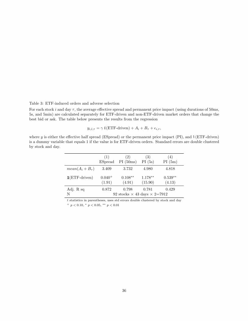
Table 3: ETF-induced orders and adverse selection

For each stock i and day τ , the average effective spread and permanent price impact (using durations of 50ms,5s, and 5min) are calculated separately for ETF-driven and non-ETF-driven market orders that change thebest bid or ask. The table below presents the results from the regression

yi,l,τ = γ 1(ETF-driven) +Ai +Bτ + εi,τ ,

where y is either the effective half spread (ESpread) or the permanent price impact (PI), and 1(ETF-driven)is a dummy variable that equals 1 if the value is for ETF-driven orders. Standard errors are double clusteredby stock and day.

(1) (2) (3) (4)ESpread PI (50ms) PI (5s) PI (5m)

mean(Ai +Bτ ) 3.409 3.732 4.980 4.818

1(ETF-driven) 0.040+ 0.108∗∗ 1.178∗∗ 0.539∗∗

(1.91) (4.91) (15.90) (4.13)

Adj. R sq 0.872 0.798 0.781 0.429N 92 stocks × 43 days × 2=7912

t statistics in parentheses, uses std errors double clustered by stock and day+ p < 0.10, ∗ p < 0.05, ∗∗ p < 0.01

36

Table 4: Cross-sectional relationship between liquidity replenishment and information asymmetry

This table presents the results from the cross-sectional regression

LRi = γ0 + γ1PETi + γ2 lmktcapi + γ3 betai + γ4 volatilityi + γ5 pricei + γ6 spreadi + εi.

LRi is the average LR value for stock i. All explanatory variables are standardized to have a mean of 0 anda standard deviation of 1. t values are calculated using heteroskedasticity-consistent standard errors.

(1) (2) (3) (4) (5)LR LR LR LR LR

constant 0.199∗∗ 0.199∗∗ 0.199∗∗ 0.199∗∗ 0.199∗∗

(33.79) (48.35) (49.39) (41.91) (46.34)

PET -0.027∗∗ -0.028∗∗ -0.021∗∗

(-4.38) (-5.94) (-3.49)

lmktcap 0.034∗∗ 0.036∗∗ 0.036∗∗ 0.040∗∗

(6.69) (7.21) (6.96) (7.98)

beta -0.003 -0.004 -0.013+ -0.011(-0.37) (-0.54) (-1.67) (-1.50)

volatility 0.019∗ 0.017∗ 0.041∗∗ 0.027∗∗

(2.62) (2.58) (5.22) (4.32)

price -0.034∗∗ -0.030∗∗ -0.028∗∗ -0.024∗∗

(-5.98) (-5.37) (-4.78) (-4.60)

spread 0.013∗ 0.024∗∗

(2.17) (5.74)

Adj. R sq 0.177 0.598 0.615 0.465 0.563N 92 92 92 92 92

t statistics in parentheses+ p < 0.10, ∗ p < 0.05, ∗∗ p < 0.01

37

Table 5: Natural experiment using index inclusion

Panel A presents the results from the first stage regression testing whether information asymmetry increaseswhen a stock is newly included in the index. y is REC or PET.

yi,τ = Ai +Bτ + γ 1(i newly included)1(τ after inclusion) + εi,τ .

Using 1(i newly included)1(τ after inclusion) as an excluded instrument, I run the 2SLS regression

LRi,τ = Ai +Bτ + γ PETi,τ + εi,τ .

Panel B presents the results. t values are calculated from standard errors clustered by stock.

Panel A: First stage regressions

level proportional standardized

(1) (2) (3) (4) (5) (6)REC PET REC PET REC PET

mean(Ai +Bτ ) 0.015 0.048 -0.032 -0.014 -0.044 -0.034

1(i new)1(τ after) 0.012∗∗ 0.021∗∗ 0.580∗∗ 0.247∗∗ 0.797∗∗ 0.614∗∗

(7.57) (6.12) (6.47) (3.97) (9.20) (4.41)

stock f.e. Yes Yes No No No No

day f.e. Yes Yes Yes Yes Yes Yes

Adj. R sq 0.839 0.764 0.053 0.200 0.082 0.400N 990 990 990 990 990 990

Panel B: Second stage regressions

(1) (2) (3)level proportional standardized

mean(Ai +Bτ ) 0.266 -0.000 -0.000

PET -1.261∗ -0.225∗ -0.227+

(-1.97) (-1.98) (-1.71)

stock f.e. Yes No No

day f.e. Yes Yes Yes

N 990 990 990

t statistics in parentheses+ p < 0.10, ∗ p < 0.05, ∗∗ p < 0.01

38

Table 6: Market volatility and liquidity replenishment

The table below presents how daily average information asymmetry and liquidity replenishment change withmarket volatility. I run

yτ = γ0 + γ1 ETFvolτ + ετ ,

where y is the cross-sectional average of PET or LR. ETF volτ is the standard deviation of 1-minute returnsof QQQ on day τ . t values are calculated using Newey-West standard errors with 5 lags.

level standardized

(1) (2) (3) (4)PET LR PET LR

constant 0.079∗∗ 0.199∗∗ 0.000 -0.000(66.02) (45.72) (0.00) (-0.00)

ETF vol 0.015∗∗ -0.019∗∗ 0.860∗∗ -0.667∗∗

(13.33) (-7.82) (13.33) (-7.82)

Adj. R sq 0.733 0.432 0.733 0.432N 43 43 43 43

t statistics in parentheses+ p < 0.10, ∗ p < 0.05, ∗∗ p < 0.01

39

Table 7: Information asymmetry sensitivity and market volatility

Below presents the results from the regression

LRi,τ = Ai + (δ0 + δ1γ1i)ETF volτ + ξi,τ .

γ1i are standardized value of γ1i, the sensitivity of stock i’s PET to market volatility. γ1i is estimated bythe following stock-by-stock regression

PETi,τ = γ0i + γ1i ETFvolτ + εi,τ

t values are calculated from standard errors that are clustered by stock and day.

(1) (2) (3)level proportional standardized

mean(Ai) 0.159 0.000 0.000

ETF vol -0.019∗∗ -0.085∗∗ -0.238∗∗

(-8.27) (-7.23) (-7.15)

γ1 × ETF vol -0.014∗∗ -0.048∗∗ -0.127∗∗

(-6.51) (-4.28) (-5.16)

stock f.e. Yes No NoAdj. R sq 0.464 0.065 0.072N 3956 3956 3956

t statistics in parentheses+ p < 0.10, ∗ p < 0.05, ∗∗ p < 0.01

40

Table 8: Stock characteristics and sensitivity to market volatility

I run the following regressionyi,τ = γ0 + (γ1 + γ2 xi)ETFvolτ + εi,τ ,

where y is PET or LR, xi are size and REC0. REC0 is calculated using data from the first five days ofthe sample, and the regression is estimated over the rest of the sample period. t values are calculated usingstandard errors clustered by stock and day.

standardized proportional

(1) (2) (3) (4) (5) (6)LR PET REC LR PET REC

ETF vol -0.244∗∗ 0.627∗∗ -0.124∗ -0.089∗∗ 0.206∗∗ -0.014(-6.79) (6.78) (-2.26) (-6.62) (7.20) (-0.59)

log mktcap × ETF vol -0.082∗∗ 0.037∗∗ 0.245∗∗ -0.017∗ 0.022∗∗ 0.152∗∗

(-3.82) (20.38) (6.11) (-2.25) (2.84) (6.39)

REC0× ETF vol 0.100∗∗ -0.053∗ -0.269∗∗ 0.031∗∗ -0.060∗∗ -0.134∗∗

(3.26) (-2.52) (-6.19) (2.81) (-6.00) (-6.38)

Adj. R sq 0.072 0.396 0.121 0.060 0.388 0.142N 3496 3496 3496 3496 3496 3496

t statistics in parentheses+ p < 0.10, ∗ p < 0.05, ∗∗ p < 0.01

41

Table 9: Cross-sectional determinants of information asymmetry

I study the cross-sectional determinants of REC and PET using the following cross-sectional regressions

RECi = γ0 + γ1 lmktcapi + γ2 betai + γ3 volatilityi + γ4 pricei + γ5 spreadi + εi

PETi = δ0 + δ1 lmktcapi + δ2 betai + δ3 volatilityi + δ4 pricei + δ5 spreadi + δ6RECi + ξi.

RECi and PETi are the average REC and PET values for stock i. All explanatory variables are standardizedto have a mean of 0 and a standard deviation of 1. t values are calculated using heteroskedasticity-consistentstandard errors.

(1) (2) (3) (4) (5) (6) (7)REC REC REC PET PET PET PET

constant 0.0199∗∗ 0.0199∗∗ 0.0199∗∗ 0.0791∗∗ 0.0791∗∗ 0.0791∗∗ 0.0791∗∗

(15.01) (17.00) (22.75) (39.47) (50.08) (52.43) (51.13)

lmktcap 0.0058+ 0.0026 0.0010 -0.0022 -0.0032+ -0.0036∗

(1.98) (1.13) (0.51) (-1.24) (-1.89) (-2.28)

beta 0.0073∗∗ 0.0065∗∗ 0.0041 0.0053+ 0.0071∗∗

(2.63) (2.76) (1.43) (1.96) (2.84)

volatility -0.0077∗∗ -0.0021 -0.0122∗∗ -0.0103∗∗ -0.0109∗∗

(-4.33) (-1.41) (-3.56) (-3.66) (-4.07)

price 0.0068∗∗ 0.0054∗∗ -0.0079∗∗ -0.0070∗∗ -0.0052∗∗

(3.24) (3.37) (-4.71) (-3.90) (-3.11)

spread -0.0099∗∗ -0.0078∗ -0.0118∗∗

(-6.01) (-2.59) (-5.58)

REC 0.0098∗∗ 0.0106∗∗ 0.0057∗

(3.96) (5.90) (2.32)

Adj. R sq 0.113 0.309 0.542 0.199 0.502 0.546 0.522N 92 92 92 92 92 92 92

t statistics in parentheses+ p < 0.10, ∗ p < 0.05, ∗∗ p < 0.01

42

Figure 5: Information asymmetry and market volatility

Daily average PET and ETFvol are plotted over the sample period. ETF volatility are calculated using1-minute ETF returns, and are rescaled to daily values.

43

Figure 6: Liquidity replenishment and market volatility

Daily average LR and ETFvol are plotted over the sample period. ETF volatility are calculated using1-minute ETF returns, and are rescaled to daily values.

44

Appendix

A Existence and Uniqueness

The Hawkes self-exciting model is determined by an intensity function of the form

λr(t) = µr(t) +

M∑m=1

∑tim<t

(a(1)rmb(1)rme

−b(1)rm(t−tim) + a(2)rmb(2)rme

−b(2)rm(t−tim)). (26)

As Embrechts et al. (2011) note, this leaves the existence and the uniqueness questions open.

Theorem 3.1 of Bowsher (2007) establishes that if, for a given parameter vector θ = (θ1, · · · , θM ) where

θr = {ar1, · · · , arM , br1, · · · , brM , µr(t)}

M∑r=1

∫ T

0

λr(t; θ) dt <∞, (27)

there exists a unique point process for the limit order book arrival process with the intensity λr(t; θ) for each

order type r. Intuitively, the sufficient condition (27) ensures that events do not happen infinitely many

times over a bounded interval.

For proof, see Bowsher (2007) and papers cited within. Embrechts et al. (2011) also show the existence

and uniqueness of DGP if the matrix (arm)r,m=1,2,··· ,M has a spectral radius smaller than 1. They only look

at cases with constant µr(t), but we can easily see that this is a sufficient condition for (27) to hold.

B Maximum Likelihood Estimation

Ogata (1978) proves that the maximum likelihood estimator is consistent and asymptotically normal for a

univariate stationary Hawkes process with a constant base intensity of µ(t) = µ. However, the Hawkes process

I use is nonstationary because µr(t) is not a constant as in the original Hawkes model (Hawkes (1971)) but a

time-deterministic function. Bowsher (2007) extends the results to nonstationary and multivariate processes

using simulations.

45

Plugging appropriate expressions into (7), the log likelihood function of event r is

lr(θr) =

∫(0,T ]

(1− λr(s|θr) ds+

∫(0,T ]

log λr(s|θr) dNr(s) (28)

= T −∫(0,T ]

µr(s) ds−M∑m=1

∑tmi

2∑j=1

a(j)rm(1− exp(−b(j)rm(T − tmi )))

+∑trl

log

µr(trl ) +

M∑m=1

2∑j=1

a(j)rmb(j)rmR

(j)rm(trl )

, (29)

where tmi is the ith event of type m and

R(j)rm(trl ) =

∑tmk <t

rl

exp(−b(j)rm(trl − tmk )). (30)

If there are multiple days, as noted in Section 3.4, each day is assumed to be an independent realization,

thus the log likelihood will be the average of all days. (30) is calculated recursively. I use a modified

Newton-Raphson method with an analytical gradient and Hessian to maximize the likelihood function.

If a(j)rm is zero or very close to zero, or if b

(j)rm is small (in other words, if the half life is too long — typically

longer than the trading day), then it complicates the estimation as the likelihood function becomes flat in

that dimension. It generally is not problematic for the point estimates, but it confounds the asymptotics.

Therefore, after the preliminary estimation, I take out the terms with a very small median a(j)rm or b

(j)rm.

Empty cells in Table 2a and 2b are terms that are taken out.

C Simultaneous events

Existence, uniqueness, and maximum likelihood estimation all require the point process (PP) to be a simple

PP, i.e., there is zero probability that two events, whether they are of the same type or not, happen at the

exact same time. This is a concern when PPs are used to study limit order book data as time stamps are

often not fine enough and many events have the same time stamp. For example, Large (2007) has 1-second

time stamps, and 40% of the observations have another event falling in the same second. Some papers thin

the data so that no two events have the same time stamp; some add random variation in time to the events

that happen in the same time stamp; and others keep it as is but with no concurrent excitations.

Fortunately, in the NASDAQ TotalView-ITCH data, observations are not only time stamped in millisec-

onds but are also sequenced. They are in the same sequence that each order was processed and also what

46

investors (or machines) that subscribe and use the feed saw. Thus, even for different tickers I can perfectly

order which observation came first. For observations that fall in the same millisecond, I equally space them

out over the millisecond. This might lead to slight overestimation of half-lives if there is clustering within

the millisecond, but the effect will be minimal.

One issue, however, is true concurrent events. For example, if a marketable limit buy order has an order

size larger than the current best ask depth but a price lower than the second best ask, it will deplete the

current best ask and the remaining order will be added to the book as a buy limit order. This type of event

is quite rare (less than 3% of market orders that change the best bid/ask, less than 0.5% of total events), so

results are not sensitive to how this issue is dealt with. Similar to Large (2007), I keep the data as is.

D Did the limit order book dynamics change?

The Hawkes model estimation also allows us to reexamine the limit order book dynamics using recent data

and to compare it to the results from the existing literature. Market microstructure has changed significantly,

yet it is not clear how the limit order book dynamics have changed. Are today’s markets just the “old markets

on steroids,” where the dynamics are mostly the same but just faster? Or are there fundamental differences?

To study conditional event frequencies, there are two different sets of state variables that we can condition

on. First are events such as changes in the limit order book. Second are those that are generally thought

of as state variables, such as bid-ask spread or volatility. The methodology in this paper naturally relates

to the first approach, but given that most state variables in the second approach change as a result of limit

order book events, the two approaches are related. For example, bid-ask spreads change if and only if there

are changes in the best bid or ask, which are considered “events” in the first framework.

Papers along the first dimension (Biais et al. (1995) and Ellul et al. (2007)) condition on the last order

type and examine the conditional probability of the next order being a particular type. They find that

there is a diagonal effect in general — market buy tends to be followed by a market buy, limit buy that is

within the best quotes tends to be followed by another such order, etc. In addition, Ellul et al. (2007) find a

liquidity exhaustion-replenishment cycle in the longer term (from couple seconds to couple minutes). Both

papers attribute the diagonal effect in market orders to follow-on strategies rather than order-splitting, since

another market order tends to arrive before liquidity is replenished. In contrast, I find that, on average,

after a market order exhausting liquidity, liquidity replenishment happens faster than another market order

coming in. For example, a market buy that increases the best ask is followed by a limit sell order that

47

decreases the ask with a 20% probability and a 1.7ms half-life; another market buy that increases the ask

with a 7% probability and a 55.7ms half-life; and a market buy that doesn’t move the ask with a 2.8%

probability and a 11ms half-life. This difference is driven by faster liquidity provision — perhaps liquidity

provision became fast enough that it is now optimal for follow-on strategies to wait slightly before submitting

orders, or order-splitting might have become more prevalent relative to follow-on strategies as depth became

lower.

The diagonal effect in limit order submission that changes the best quotes found in Biais et al. (1995)

and Ellul et al. (2007) is not as strong in the recent data. This is somewhat surprising if the diagonal effect

in limit order addition is due to multiple limit order providers undercutting each other for price priority (as

in Yeo (2006)), as we would think that computers made undercutting much easier. One possible explanation

is that bid-ask spreads are smaller today, making undercutting in succession more difficult, as a limit order

that changes the best price by definition decreases the spread.

On the other hand, the diagonal effect in limit order cancellation that changes the best quotes is quite

strong. This has not been directly studied in earlier research, as all cancellations are generally grouped into

one category regardless of whether they change the best quote.

Another distinct result that emerges is a pattern of order submissions and cancellations, especially on

the same side, exciting each other. This is not completely new, as many papers (Biais et al. (1995), Ranaldo

(2004), Griffiths et al. (2000)) show that large bid-ask spreads attract limit orders. What is new, however, is

that this effect is very fast and that cancellation (submission) is more likely to excite same-side submission

(cancellation) than the opposite-side one. For example, if there a bid improvement, it is quite likely (5%) to

be cancelled quickly (a 6.2ms half life), less so for an ask to be cancelled (2.7% with a 3.8ms half life); and

if there is a cancellation on the bid side, it is likely (26%) to be re-filled quickly (a 3.2ms half life) on the

bid side compared to the ask side (8.2% with a 3.6ms half life). This phenomenon is likely due to the use of

fleeting orders by HFTs.

After a market buy that increases the ask, the best bid tends to increase. Biais et al. (1995) also document

this “comovement” effect (as termed by Rosu (2009)), and this effect is quite strong in their results, although

slightly less so than the diagonal effect (a market buy is more likely to be followed by a market buy than

by an increase in the bid). In my results, if the slower reaction term is included (the half-life of the slower

term of this comovement effect is still quite fast at 61ms), a market buy is followed by an increase in bid

in 50% of the cases; this is the strongest reaction to a market buy. Biais et al. (1995) argue that this

comovement effect is due to the information content of the trade, similar to the market maker updating in

48

Glosten and Milgrom (1985). Parlour (1998) and Rosu (2009), however, argue that this can be explained

without information asymmetry. Although cancellations are not modeled, since the effect arises from the

number of outstanding bid and ask quotes in both papers, a cancellation of a limit sell order that increases

the ask (CA) should have the same effect as a market buy that increases the ask (MB). However, in my

results, a bid increases much more in reaction to action MB than to action CA; the comovement effect is

thus more naturally interpreted as a consequence of the information content of market orders, and market

orders must contain more information than cancellations.

Finally, liquidity takers also seem to monitor the market closely and submit market buy orders right after

ask decreases and market sells after bid increases. This is consistent with Hendershott and Riordan (2012),

who finds that algorithmic traders consume liquidity when it is cheap.

What emerges is a fast, complicated, and dynamic process, in which both positive and negative feedback

forces are present, and reactions to market orders are strongest. Both the liquidity providers and takers

seem to monitor the market actively and react quickly. Most dynamic models of limit order book assume

a constant arrival rate of buyers and sellers. Consequently, many of their predictions on dynamics are

implicitly derived from the arithmetic identity in which an increase in market buys must mean that limit

buy submissions decrease. Although this paper does not offer a formal statistical test, my results suggest

that this assumption does not hold for HFTs.

E Incorrect Half-life

In Section 3.4, I fix the half-lives to be the same across all stocks and days and let the size of the effect (arm)

vary. The size and the half-life of the effect are two separate dimensions, and I fix the half-life to be constant,

assuming that the size of the effect is the only dimension that changes. If the probability of effect happening

stays the same but the effect becomes slower, will this make the interpretations of the estimations from the

incorrectly specified model invalid? Intuitively, if the probability of the effect happening remains constant

at 10% and the half-life increases from 1s to 3s, but if I assume a 1s constant half-life, the probability of the

effect happening would seem smaller because I am looking at a shorter period of time than I should. Thus,

arm would be estimated to be smaller than 10%. Results from the paper could still be interpreted similarly

as if I used the true model to estimate, since a longer half-life and a lower probability of the effect happening

both point to less involvement by the HFTs.

I test the above idea using simulations. I simulate a simple case with two actions (M = 2) and J = 1.

49

For the first set of simulations, I use the parameters

a =

0.1 0

0.1 0.1

, b =

log(2)2 0

log(2)4

log(2)2

, λ0 =

0.1

0.1

, (31)

where element a(r,m) refers to arm and b(r,m) refers to brm. The half-lives of both self-excitations are 2,

the half-life of event 1 precipitating event 2 is 4, and event 2 does not precipitate event 1. b1,2 is written

as 0 for convenience, but the value does not matter as a1,2 = 0. Now if we have incorrectly assumed that

b2,1 = log(2)2 (i.e., that the half-life of event 1 precipitating event 2 is 2), thus

b =

log(2)2 0

log(2)2

log(2)2

, (32)

and estimated a using b, this means that we have assumed a shorter half-life than the true value. I assume

a length of 5,000 for each simulation (T = 5, 000) and simulate 10,000 times using the above parameters. I

also do the same using a different set of parameters that are closer to the estimates from the data.

a =

0.1 0.05

0.2 0.01

, b =

log(2)4 log(2)× 10

log(2)× 2 log(2)

, λ0 =

0.1

0.1

(33)

and

b =

log(2)4 log(2)× 10

log(2)× 10 log(2)

. (34)

In this case, the half-life of the cross-excitation of event 1 on 2 is mistaken as 0.1 instead of 0.5, the true

value. Simulations are done using a modified version of Ogata (1981)’s thinning algorithm. A modified

version of the algorithm for a multivariate Hawkes process is outlined and proved in Bowsher (2007).

Figure 7 presents the distribution of estimated a2,1 for both parameters. Comparing (a) with (b) and

(c) with (d), we can observe that under the incorrect assumption of shorter half-life, a’s are estimated to be

smaller than the true values.

50

Figure 7: Histogram of a2,1 estimates from simulated data

Panel (a) and (b) are estimates from simulated data using parameters in (31), (c) and (d) are using (33).Panel (a) and (c) are estimated using incorrect b values, (32) and (34), respectively. Panel (b) and (d) areestimates using correct b values for comparison. True a2,1 is 0.1 for (a) and (b), and 0.2 for (c) and (d).

51

F Potential issues with the Hawkes model and the REC measure

One issue with the Hawkes model is that it might seem as if event m excites event r if their intensity processes

are correlated even without one really causing the other. If the intensity of event type 1 and 2 are

λ1(t) = d1 ψc(t) + ψ1(t) (35)

λ2(t) = d2 ψc(t) + ψ2(t), (36)

where ψc(t) is a common latent process, a1,2 and a2,1 appear positive in the Hawkes model. We thus would

incorrectly interpret the estimates from the Hawkes model as event 1 and 2 mutually exciting each other.

Here I divide all possible scenarios by whether the two events are of the same direction and by how fast the

ψc(t) mean reverts, and address them one by one.

If event 1 and 2 are both events in the stock, and if the two events are in the opposite direction (one

increases price, another decreases), then it seems unlikely that they would be governed by a common latent

process unless they directly affect each other. For example, event MB (market buy) tends to be followed by

AA (add ask), and vice versa, but it would not make sense to think that when traders tend to submit market

buys, traders also tend to improve the ask. Rather, it is because someone submitted a market buy that

increased the ask that someone else submits a limit sell order that brings the ask back down, or it is because

someone submitted an ask that is below the current best ask that someone else seized the opportunity and

transacted against the new, better ask quote.

If the events are in the same direction, it is plausible that there would be a common latent component.

If, in the estimation results, event 1 excites event 2, but not the other way around, it is unlikely that the

results are due to a common component. For example, event MB (market buy) triggers event CA (cancel

ask), but not the other way around. However, if it is merely the case that one effect is larger than the other,

it may be because d1 and d2 from (35) and (36) are different.

In the case where event 1 and 2 appears to mutually excite each other, we can divide the cases by the

speed of mean reversion in the common component ψc(t). Recall the Hawkes model specification

λr(t) = µr(t) +

M∑m=1

∑tmi <t

(a(1)rmb(1)rme

−b(1)rm(t−tmi ) + a(2)rmb(2)rme

−b(2)rm(t−tmi )), (37)

where the intensity has three components: slowly changing base intensity µr(t) (in hours), very fast com-

ponent (in milliseconds), and slower component (usually in seconds or minutes). Therefore, if the mean

52

reversion rate of ψc(t) is very slow (in hours) or is not mean reverting at all, it will be captured in the base

intensity. If it is faster, it will appear in one of the two interaction terms. Intuitively, if the model specified

by (35) and (36) is correct but we estimate the Hawkes model instead, the estimated half-life would be of a

similar magnitude to that implied by the speed of mean reversion of ψc(t). (This point will be shown later

via simulations.) If the mean reversion rate is thus moderate (minutes or seconds), it will appear in the

second interaction term a(2)rmb

(2)rme−b

(2)rm(t−tmi ). Only if it is in milliseconds will it appear in the first interaction

term a(1)rmb

(1)rme−b

(1)rm(t−tmi ), which is the only one that would be relevant since I mostly focus on a

(1)rm and b

(1)rm.

When would it be the case that ψc(t) mean reverts very fast, in milliseconds? Since virtually all stories of

real news or sentiment would predict a much slower mean reversion, it must also be hard information, such

as futures index prices, that is driving ψc(t). For example, it may be the case that both event MB (market

buy) and ETF↑ (increase in ETF ask) are driven by futures price increase, but neither of the two drives the

other nor is one faster than the other. In this case, it will still seem as if ETF↑ excites MB, and vice versa,

according to the Hawkes model. However, I can redefine the futures price to be the hard information, and

the size of the effect estimated would be an underestimate of the true value. In this sense, I can relax the

assumption made in Section 4.1 that the information from futures must flow first into ETF and then into

stocks. Therefore, the intuition for the REC measure stays the same since the estimates from the Hawkes

model measure the reaction to some other hard information, most likely futures price.

To show that the common component ψc(t) has to be extremely quickly mean-reverting in order for

the estimated half-life of the Hawkes model to be in milliseconds, I simulate a simple case of the scenario

described above by (35) and (36) with two processes having the same intensity

λ1(t) = λ2(t) = ψc(t), (38)

where ψc(t) has Poisson-arriving jumps that decay exponentially at a rate b

ψc(t) = µ+∑τi<t

abe−b(t−τi). (39)

τi is the ith jump time, and τ is a Poisson process with intensity π. We can interpret this setting as an event

happening at each jump time τ , in which the events are observable to the traders but not to the researcher.

Traders react to these events with action 1 or 2, and we only observe these actions in the data.

53

I simulate using parameters

a = 0.5, µ = 0.1, π = 0.2 (40)

b = log 2 or log 2/10. (41)

b of log 2 implies that the half-life of each jump is 1, and log 2/10 implies a half-life of 10. I estimate the

Hawkes model on each simulation, and present the half-life of cross-excitation (event 1 exciting event 2) in

Table 10 based on 1,000 simulations. Results show that the slower the mean-reversion of the latent common

component, the longer the estimated half-life of the cross-excitation, and that they are of the same magnitude.

This result, of course, may also depend on the parameter values or the functional form of the latent common

process ψc(t). However, it is generally difficult to get a very short half-life with other functional forms of

ψc(t) with a reasonable mean intensity.

Table 10: Estimated half-life of cross-excitation in the Hawkes model

10% 25% 50% 75% 90%

b = log 2 0.41 0.62 0.91 1.34 2.59b = log 2/10 1.96 4.56 10.24 29.12 157.15

G Potential issues with the PET measure

The PET measure faces a similar problem as above: if, for example, the intensities of event MB (market

buy) and ETF↑ (increase in ETF ask) are

λMB(t) = d1ψc(t) + ψMB(t) (42)

λETF↑(t) = d2ψc(t) + ψETF↑(t), (43)

PET will be positive although ETF↑ does not excite MB. Unfortunately, it is not possible to make the same

argument as in the REC measure, because the PET measure is not constructed from the Hawkes model.

Even if the mean reversion rate for the common latent process ψc(t) is slow, it will still make PET positive.

One robustness test is to check against the REC measure since REC is not subject to this issue, as shown

in Appendix F. As shown in Section 4.1, PET and REC are positively correlated in the cross section, thus

mitigating this concern.

54

Checking against the REC measure in the time series, however, is troublesome. When hard information

comes out more frequently, aggressive HFTs may act on fractionally less of the information (i.e., REC

decreases), but from the point of view of the liquidity provider, a higher fraction of market orders may be

informed (i.e., PET increases). I thus present another robustness test using an alternative PET measure

that is significant if and only if the mean reversion of the common latent component ψc(t) is very fast.

If we plot the distribution of event MB around event ETF↑, the distribution would look different, depend-

ing on the mean reversion rate of ψc(t). As in Figure 8, the distribution would be flat if ψc(t) mean-reverts

slowly or does not mean revert but would exhibit a much stronger hump-shaped pattern if ψc(t) mean-reverts

rapidly. Therefore, I measure À−Á in Figure 8 to distinguish the two cases. The PET measure used in the

paper corresponds to À in Figure 8.

ETF↑ 0.05 0.1

À Á

ETF↑ 0.05 0.1

À Á

(a) Slow or moderate (b) Fast

Figure 8: Illustration of distribution of event MB around event ETF↑(a) illustrates the case when the common latency component ψc(t) mean-reverts slowly, and (b) when itmean-reverts fast. Units are in seconds, thus 0.05 and 0.1 are 50ms and 100ms, respectively.

Recall from (12) how PET was measured, and define longPET in the same manner but using a 100ms

window to define “ETF-driven” and “opposite” from Figure 4. To measure À−Á, I define PET2 as

PET2i,τ = PET − longPETi,τ . (44)

If ψc(t) is not driven by hard information, PET2 should be zero on average and independent of PET. If

it is largely driven by hard information, PET and PET2 will be strongly correlated. Figure 9 confirms that

the latter is the case.

55

Figure 9: PET and PET2

Panel (a) is the pooled level data using raw values of PET and PET2. Panel (b) focuses on within dayvariation, where I subtract the daily mean and divide by the daily standard deviation. Panel (c) presentswithin-stock variation, where I subtract the stock-specific mean and divide by the stock-specific standarddeviation.

56