machine learning to improve natural gas reservoir simulations

Machine Learning to Improve Natural Gas Reservoir Simulations

Abouzar Choubineh

[Corresponding Author]

Department of Applied Mathematics, Xi'an Jiaotong-Liverpool University, Suzhou, P. R. China

Department of Computer Science, University of Liverpool, Liverpool, United Kingdom

[email protected] – [email protected]

Jie Chen


[email protected]

Frans Coenen

Department of Computer Science, University of Liverpool, Liverpool, United Kingdom

[email protected]

Fei Ma


[email protected]

David A. Wood

DWA Energy Limited, Lincoln, United Kingdom

[email protected]

ORCID: 0000-0003-3202-4069

mailto:[email protected]




Banner headline [75 words]

Reservoir simulation methods applied to gas reservoirs are reviewed and the key influencing

variables identified. Machine Learning (ML) methods can be applied in various ways to improve

the performance of gas reservoir simulations, especially in respect to history matching and proxy

modeling. Additionally, ML can assist the CO2 sequestration and enhanced gas recovery, well

placement optimization, production optimization, estimation of gas production, dew point

prediction in gas condensate reservoirs, and pressure and rate transient analysis.

Abstract

Natural gas reservoir simulation, as a physics-based numerical method, needs to be carried out

with a high level of precision. If not, it may be highly misleading and cause substantial losses, poor

estimation of ultimate recovery factor, and wasted effort. Although simple simulations often

provide acceptable approximations, there is a continued desire to develop more sophisticated

simulation strategies and techniques. Given the capabilities of Machine Learning (ML) and their

general acceptance in recent decades, this chapter considers the application of these techniques to

gas reservoir simulations. The aspiration ML technics should be capable of providing some

improvements in terms of both accuracy and speed. The simulation of gas reservoirs (dry gas, wet

gas and retrograde gas-condensate) is introduced along with its fundamental concepts and

governing equations. More specific and advanced concepts of applying ML in modern reservoir

simulation models are described and justified, particularly with respect to history matching and

proxy models. Reservoir simulation assisted by machine learning is becoming increasingly applied

to assess suitably of reservoirs for carbon capture and sequestration associated with enhanced gas

recovery. Such applications, and the ability to improve reservoir performance via production

efficiency, make ML-assisted reservoir simulation a valuable approach for improving the

sustainability of natural gas reservoirs. The concepts are reinforced using a case study applying

two ML models providing dew point pressure predictions for gas condensate reservoirs.

Keywords: Reservoir simulation; Natural gas; Machine learning; Reservoir characterization;

Mathematical models; History matching; Proxy modeling; Optimization; Dew point pressure.

1. Introduction

Petroleum reservoirs can be classified into oil and gas reservoirs with respect to their phase

behavior; typically illustrated on a pressure-temperature (P-T) diagram. If the reservoir

temperature exceeds the critical temperature of the hydrocarbon fluid, it is regarded as a natural

gas reservoir. Gas reservoirs are separated into three groups: (i) dry gas, (ii) wet gas, and (iii)

retrograde gas-condensate reservoirs. To distinguish these three distinctive reservoirs, the

cricondentherm point is defined. It is the maximum temperature above which no liquid is produced

no matter how high the pressure becomes. In both dry gas and wet gas, the reservoir temperature

is more than the hydrocarbon system cricondentherm. Dry gas reservoirs always remain in the gas

phase. However, some liquid is formed at the surface conditions when fluids are produced from

wet gas reservoirs. When the reservoir temperature is between critical temperature and

cricondentherm, the reservoir is considered as a special case, i.e., described as a retrograde gas-

condensate reservoir [1].

Reservoir simulation is a strategy, or set of techniques, by which a numerical model of the

geophysical and geological characteristics of a subterranean resource, and the (single phase or

multiphase) fluid system is used to investigate and predict how the available fluids flow through a

porous and permeable medium into the stock tank. It is very hard to perceive the fluid behavior in

a reservoir, describe the physical and chemical processes, and measure or estimate variables that

affect the flow behavior. Forecasting how fluid flow from a reservoir proceeds under various drive

mechanisms over time, and how it reacts to the application of various improved and enhanced

recovery techniques is always associated with a degree of uncertainty. Reservoir simulation began

in 1936 by developing the Material Balance Equation (MBE) for petroleum reservoirs. The MBE

remains a standard tool for the prediction of the fluid flow inside many types of petroleum reservoir

[2].

Machine learning algorithms search for complex patterns among large numbers of data records.

Whilst other industries, such as telecommunication, banking, and automotive have experienced

considerable benefits, the utilization of ML in the petroleum engineering has only been exploited

by larger operators and service companies on commercial scales over the past decades or so. In

our context, the use of ML technology along with an astounding increase in computer power can

provide far more sophisticated reservoir simulations with a high degree of granulation than was

possible just a few years ago. Well-constructed ML models help to reduce the uncertainty

associated with the simulation process and consequently, produce more accurate predictions of

fluid flow and ultimate resource recovery.

In Section 2, we present the basic concepts concerning reservoir simulation. Section 3 summarizes

the importance of ML techniques in modern reservoir simulation models and highlights some of

the challenges and more advanced approaches and strategies that help to overcome them. Section

4 describes the case study addressing the simulation of a substantial gas-condensate reservoir.

2. Fundamental concepts and key principles

We begin by describing the five stages involved in constructing a gas reservoir simulation model.

The governing equations typically used in the simulation process are then reviewed and explained.

2.1. Reservoir simulation

Why do we need to create reservoir simulation models? There are in fact several benefits from

doing so. The main purpose is to forecast the performance of reservoirs (here natural gas) at any

future point in time and to optimize the petroleum fluid recovery factors under different operating

conditions and with development and injection wells potentially drilled at different locations and

at different times over the production life of a reservoir. To this end, inputs from experts in geology

with three-dimensional perspectives, physics, drilling, petroleum and reservoir engineering,

mathematics and computer science are needed (Figure 1). From a specific point of view and based

on [3], reservoir simulation is commonly conducted in five stages: (i) define the simulation

objectives, (ii) collect and validate the required data, (iii) design the reservoir simulator using

appropriate software, (iv) tune and validate the developed model(s) using techniques such as

history matching to ensure that it is robust and reliable, and (v) apply the models to make accurate

predictions and test various field development plans.

Figure 1 (a) Multi-dimensional inputs required to develop a three-dimensional reservoir

simulation model and progress it from static to a dynamic analysis of fluid movement.

Figure 1 (b) The initial static reservoir model has to capture, with high granularity via its dense

arrangement of cellular components, the three-dimensional structure, porosity and permeability

of the mapped reservoir.

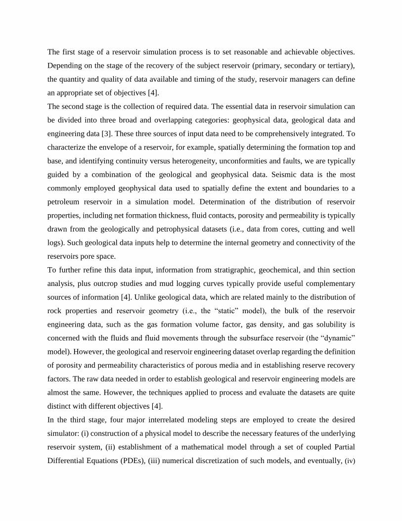
The first stage of a reservoir simulation process is to set reasonable and achievable objectives.

Depending on the stage of the recovery of the subject reservoir (primary, secondary or tertiary),

the quantity and quality of data available and timing of the study, reservoir managers can define

an appropriate set of objectives [4].

The second stage is the collection of required data. The essential data in reservoir simulation can

be divided into three broad and overlapping categories: geophysical data, geological data and

engineering data [3]. These three sources of input data need to be comprehensively integrated. To

characterize the envelope of a reservoir, for example, spatially determining the formation top and

base, and identifying continuity versus heterogeneity, unconformities and faults, we are typically

guided by a combination of the geological and geophysical data. Seismic data is the most

commonly employed geophysical data used to spatially define the extent and boundaries to a

petroleum reservoir in a simulation model. Determination of the distribution of reservoir

properties, including net formation thickness, fluid contacts, porosity and permeability is typically

drawn from the geologically and petrophysical datasets (i.e., data from cores, cutting and well

logs). Such geological data inputs help to determine the internal geometry and connectivity of the

reservoirs pore space.

To further refine this data input, information from stratigraphic, geochemical, and thin section

analysis, plus outcrop studies and mud logging curves typically provide useful complementary

sources of information [4]. Unlike geological data, which are related mainly to the distribution of

rock properties and reservoir geometry (i.e., the “static” model), the bulk of the reservoir

engineering data, such as the gas formation volume factor, gas density, and gas solubility is

concerned with the fluids and fluid movements through the subsurface reservoir (the “dynamic”

model). However, the geological and reservoir engineering dataset overlap regarding the definition

of porosity and permeability characteristics of porous media and in establishing reserve recovery

factors. The raw data needed in order to establish geological and reservoir engineering models are

almost the same. However, the techniques applied to process and evaluate the datasets are quite

distinct with different objectives [4].

In the third stage, four major interrelated modeling steps are employed to create the desired

simulator: (i) construction of a physical model to describe the necessary features of the underlying

reservoir system, (ii) establishment of a mathematical model through a set of coupled Partial

Differential Equations (PDEs), (iii) numerical discretization of such models, and eventually, (iv)

design of corresponding computer algorithms to solve the algebraic equations and optimize their

performance and aid their interpretation [4].

The fourth stage of the reservoir simulation process is the tuning of the model created to better

replicate reservoir conditions. Unlike a forward-looking forecasting type of exercise, which

engages a set of reservoir model parameters to predict its performance, backward-looking history

matching provides a useful benchmark to validate a reservoir simulation; i.e., to confirm that it can

replicate the production performance (i.e., volumes and flow rates from specific reservoir

compartments) actually recorded and observed. This is the inverse of a forecasting exercise. In

other words, it is an essential stage to modify uncertain model variables, such as porosity,

permeability and water: gas ratio, and reservoir spatial heterogeneities, drive mechanisms, etc., in

a way that the final model(s) are able to appropriately reproduce the past dynamic response of a

real reservoir. More specifically, basic factors like historical production rates, water cuts, fluid

saturations and pressures are matched as closely as possible. If a model is unable to do this

accurately, its credibility is undermined before forward-looking analysis commences.

Following the history matching and performance validation, the prediction of the future

performance of a reservoir can begin (Stage 5). Among the available operating strategies and infill

drilling programs, assessing their benefits and drawbacks, reservoir managers have to select

options that would likely to the most profitable and sustainable performance ensuring that

petroleum fluid recovery is maximized over the production life of the reservoir.

Reservoir performance prediction is also achievable applying classical techniques that exploit

analogues, conduct experiments and evaluate mathematical models [4]. The first uses properties

of mature reservoirs similar to the specified reservoir. Experimental methods use measured

properties, such as pressure, flow rate and fluid saturation(s) and then scale them up to approximate

the entire petroleum accumulation. The third category employs material balance, statistical

analysis, decline curve fitting and other analytical techniques, these methods have similar

objectives to reservoir simulation and, indeed some are used to help verify some of the outputs of

simulation models (e.g., decline curve fitting for well flow rates and fluid reservoirs). For instance,

permeability can be estimated via a pressure build-up analysis, or acquiring some information on

water encroachment over time and the size of the aquifer during history matching. It is also

possible to apply material balance calculations to estimate resource recovery volumes to compare

with reservoir simulation model forecasts [4].

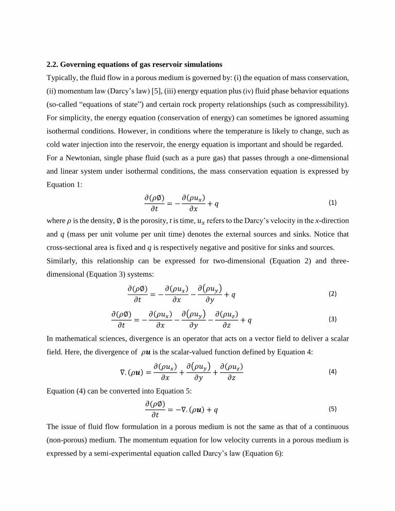
2.2. Governing equations of gas reservoir simulations

Typically, the fluid flow in a porous medium is governed by: (i) the equation of mass conservation,

(ii) momentum law (Darcy’s law) [5], (iii) energy equation plus (iv) fluid phase behavior equations

(so-called “equations of state”) and certain rock property relationships (such as compressibility).

For simplicity, the energy equation (conservation of energy) can sometimes be ignored assuming

isothermal conditions. However, in conditions where the temperature is likely to change, such as

cold water injection into the reservoir, the energy equation is important and should be regarded.

For a Newtonian, single phase fluid (such as a pure gas) that passes through a one-dimensional

and linear system under isothermal conditions, the mass conservation equation is expressed by

Equation 1:

𝜕(𝜌∅)

𝜕𝑡= −

𝜕(𝜌𝑢𝑥)

𝜕𝑥+ 𝑞 (1)

where 𝜌 is the density, ∅ is the porosity, t is time, 𝑢𝑥 refers to the Darcy’s velocity in the x-direction

and q (mass per unit volume per unit time) denotes the external sources and sinks. Notice that

cross-sectional area is fixed and q is respectively negative and positive for sinks and sources.

Similarly, this relationship can be expressed for two-dimensional (Equation 2) and three-

dimensional (Equation 3) systems:

𝜕(𝜌∅)

𝜕𝑡= −

𝜕(𝜌𝑢𝑥)

𝜕𝑥−

𝜕(𝜌𝑢𝑦)

𝜕𝑦+ 𝑞 (2)

𝜕(𝜌∅)

𝜕𝑡= −

𝜕(𝜌𝑢𝑥)

𝜕𝑥−

𝜕(𝜌𝑢𝑦)

𝜕𝑦−

𝜕(𝜌𝑢𝑧)

𝜕𝑧+ 𝑞 (3)

In mathematical sciences, divergence is an operator that acts on a vector field to deliver a scalar

field. Here, the divergence of 𝜌𝒖 is the scalar-valued function defined by Equation 4:

∇. (𝜌𝒖) =𝜕(𝜌𝑢𝑥)

𝜕𝑥+

𝜕(𝜌𝑢𝑦)

𝜕𝑦+

𝜕(𝜌𝑢𝑧)

𝜕𝑧 (4)

Equation (4) can be converted into Equation 5:

𝜕(𝜌∅)

𝜕𝑡= −∇. (𝜌𝒖) + 𝑞 (5)

The issue of fluid flow formulation in a porous medium is not the same as that of a continuous

(non-porous) medium. The momentum equation for low velocity currents in a porous medium is

expressed by a semi-experimental equation called Darcy’s law (Equation 6):

𝑢𝑥 = −𝑘𝑥

𝜇(𝜕𝑝

𝜕𝑥− 𝜌𝑔

𝜕ℎ

𝜕𝑥)

𝑢𝑦 = −𝑘𝑦

𝜇(𝜕𝑝

𝜕𝑦− 𝜌𝑔

𝜕ℎ

𝜕𝑦)

𝑢𝑧 = −𝑘𝑧

𝜇(𝜕𝑝

𝜕𝑧− 𝜌𝑔

𝜕ℎ

𝜕𝑧)

(6)

where k, 𝜇 and p are permeability, viscosity and pressure, respectively. It is common to ignore the

term containing density (𝜌), gravitational acceleration (g) and depth (h).

The gradient operator for p is marked with ∇p in the form of Equation 7:

∇p = (𝜕𝑝

𝜕𝑥,𝜕𝑝

𝜕𝑦,𝜕𝑝

𝜕𝑧) (7)

As a more general form this is expressed as Equation 8:

𝒖 = −𝒌

𝜇∇p (8)

where 𝒖 = (𝑢𝑥, 𝑢𝑦, 𝑢𝑧) and k is a diagonal tensor (𝑘𝑥, 𝑘𝑦, 𝑘𝑧). At least initially, we suppose the

porous medium is isotropic i.e., 𝑘𝑥 = 𝑘𝑦 = 𝑘𝑧, which leads to Equation 9:

𝜕(𝜌∅)

𝜕𝑡= ∇. (

𝜌

𝜇𝒌∇p) + 𝑞 (9)

Equation 9 can then be expressed as Equation 10:

(∅𝜕𝜌

𝜕𝑝+ 𝜌

𝜕∅

𝜕𝑝)

𝜕𝑝

𝜕𝑡= ∇. (

𝜌

𝜇𝒌∇p) + 𝑞 (10)

However, it is typically not reasonable to assume that gas compressibility remains constant.

Instead, Equation 11 is required:

𝐶𝑔 =1

𝜌

𝑑𝜌

𝑑𝑝=

1

𝑝−

1

𝑍

𝑑𝑍

𝑑𝑝 (11)

By taking into consideration the real gas law, and molecular weight, gas compressibility factor,

universal gas constant and temperature respectively by MW, Z, R and T, pressure can be usefully

established with Equation 12:

𝜌 =𝑝𝑀𝑊

𝑍𝑅𝑇 (12)

Where more than one phase is involved, 𝑆𝛼 the fluid phase saturation is defined as the fraction of

the whole void volume of a porous medium occupied by that specific fluid. All the available fluids

together fill the entire void spaces leading to Equation 13:

∑ 𝑆𝛼 = 1 𝛼 = 𝑔𝑎𝑠 (𝑔), 𝑤𝑎𝑡𝑒𝑟 (𝑤) 𝑎𝑛𝑑 𝑐𝑜𝑛𝑑𝑒𝑛𝑠𝑎𝑡𝑒 (𝑙) (13)

Another term related to multiphase flow is capillary pressure derived in terms of Equation 14:

𝑝𝑐𝑔𝑤 = 𝑝𝑔 − 𝑝𝑤

𝑝𝑐𝑙𝑤 = 𝑝𝑙 − 𝑝𝑤 (14)

To model the phase velocity, Darcy’s law for single phase system is expanded to consider

multiphase flow by applying Equation 15:

𝒖𝛼 = −𝒌𝛼

𝜇𝛼∇𝑝𝛼 (15)

where 𝒌𝛼 is the phase permeability, which is equal to the phase relative permeability multiplied

by the absolute permeability i.e., 𝑘𝑟𝛼𝒌, resulting in Equation 16:

𝜕(𝜌𝛼∅𝑆𝛼)

𝜕𝑡= −∇. (𝜌𝛼𝒖𝛼) + 𝑞𝛼

𝜕(𝜌𝛼∅𝑆𝛼)

𝜕𝑡= ∇. (

𝜌𝛼

𝜇𝛼𝒌𝛼∇𝑝𝛼) + 𝑞𝛼

(16)

To solve the mathematical models described, it is necessary to specify boundary and initial

conditions. Boundary Conditions (BCs) exert a set of extra constraints to the problem on prescribed

boundaries. There are typically three types of BC: Dirichlet (the first kind), Neumann (the second

kind) and Robin or Dankwerts (the mixed or third kind). In the first type, a value is assigned to the

dependent parameter(s) (for example, pressure) while the derivative of the dependent variable(s)

is known in Neumann’s condition. Robin’s boundary condition is a weighted combination of the

first two BCs. An Initial Condition (IC) refers to a value of a parameter at t=0 in the dynamic

simulation models.

Analytical solutions for this system of equations can be determined for relatively simple reservoirs

(i.e., by making multiple assumptions). An alternative is to make use of numerical solutions, such

as the finite difference method, finite element method, finite volume method, spectral method and

meshless method. For details of these numerical solutions, see [3].

3. Advanced research / field applications

As a subset of Artificial Intelligence (AI), Machine Learning (ML) is a field of study that aims to

enable systems (namely computers and robots) to learn appropriate responses and/or

interpretations directly from data. Machine learning algorithms involve computational methods to

find patterns in datasets with many thousands of data records. The most prevalent ML tool for

modelling non-linear systems is the Artificial Neural Network (ANN) [6]. Adaptive Neuro Fuzzy

Inference System (ANFIS) [7], Support Vector Machine (SVM) [8] and Least-Squares Support

Vector Machine (LSSVM) [9] are other commonly used neural-network-exploiting ML

algorithms.

Machine learning algorithms are commonly categorized by how the algorithm learns from the

available data. There are four general methods: supervised, unsupervised, semi-supervised, and

reinforcement. Using supervised learning, the training is conducted via labeled instances, while in

the case of unsupervised learning unlabelled data is used. ANN, ANFIS, SVM and LSSVM are all

supervised ML algorithms. Semi-supervised learning uses a small amount of labelled data from

which further labelled data is extrapolated. Reinforcement learning uses a generate and test

approach to maximize some reward and tends to be concerned more with optimization. Notice that

the labelling can comprise either continuous or/and discrete values. Machine learning is

penetrating many fields, including many technical and commercial applications in the gas and oil

industry [10-16].

In the context of gas reservoir simulations, ML has application in four different areas: (i) data

preprocessing, (ii) governing equations and numerical solutions, (iii) history matching and (iv)

proxy modeling. Each is discussed in further detail in the following four subsections.

3.1. Application of ML in data preprocessing and prediction of properties

The successful application of ML in reservoir simulation begins with correctly collecting,

compiling and preprocessing the raw data. Both field (geophysical and petrophysical) and

experimental (geological and engineering) data are required. However, data-collecting

methodologies are somewhat loosely controlled in gas reservoir simulations. This can lead to

producing out-of-range, duplicate, missing and unstructured data records. Entering such data into

a simulator are likely to yield misleading results. The application of ML to data preprocessing

assists in improving the quality of data to promote the extraction of better insights from the data.

Furthermore, multiple sources of data sometimes need to be integrated to best estimate a variable’s

value. Rolon et al. [17] provide a useful example of how raw data can be effectively preprocessed

in this manner. The researchers applied a generalized regression neural network to develop

synthetic well logs using information from four natural gas wells in the Upper Devonian of

Southern Pennsylvania, taking input data from gamma ray, neutron, density and resistivity well

logs. Three scenarios were considered. The only output of the first scenario was the resistivity log

while the inputs were density, neutron and gamma ray logs, the coordinates and depths. In the

second, the output of the previous stage was replaced with the density log. The neutron log was

selected as the output for the third scenario. The results confirmed the development of synthetic

logs with a reasonable degree of precision.

In addition to quality, the availability of sufficient data is also necessary for conducting a high-

quality simulation study. Modern data recording technologies during drilling (i.e., sensing while

drilling, logging while drilling and measurement while drilling) have paved the way for acquiring

massive datasets with often high dimensionality during drilling operations. It is a necessity, for the

purpose of extracting helpful and practical knowledge from these data, to successfully characterize

reservoir properties. Despite partly solving some complicated problems of reservoir engineering,

the issue of optimal features selection still remains a basic challenge. Engineers and geologists are

often willing to apply linear assumptions to select features, replacing the suspected absence of

non-linear data. As a specific example, consider the existence of different “expert opinions” on the

features needed for the prediction of reservoir rock properties. For instance, researchers propose

various sets of features for a specific output, for example nine input variables were used in [18],

while only three in [19] for the estimation of permeability. The optimality achieved therefore local

to the dataset and cannot be applied globally.

Ensemble learning can be helpful in this regard. Ensemble learning is a ML paradigm which takes

advantage of several base (or weak) learners to train a model. Unlike common ML methods that

learn only one hypothesis from a training data set, ensemble techniques attempt to develop multiple

hypotheses and then to combine them [20]. Specific to our topic, ensemble learning is capable of

incorporating the result of various base learners fed with distinct locally optimal features to

construct a single ensemble hypothesis with a global flavor. For instance, an ensemble model for

the prediction of natural gas reservoir properties was developed to choose the optimal input

features by Anifowose et al. [21]. Various instances of the ensemble learner were fed with

variables chosen from multiple bootstrap samplings of the real field data. Based on the results, the

novel model outperformed existing techniques.

In the absence of field and experimental data, ML techniques can be effectively applied to extract

fluid and rock properties. For example, Zendehboudi et al. in [22] presented a particle swarm

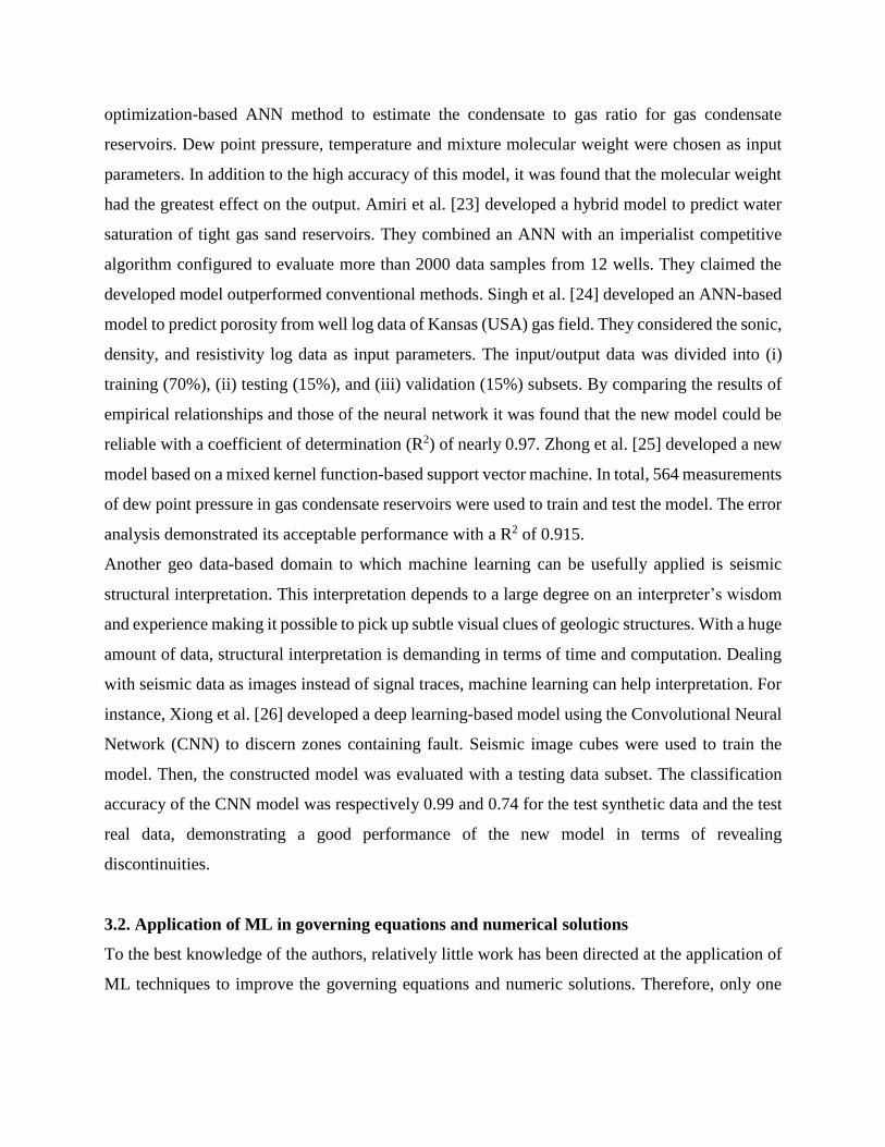
optimization-based ANN method to estimate the condensate to gas ratio for gas condensate

reservoirs. Dew point pressure, temperature and mixture molecular weight were chosen as input

parameters. In addition to the high accuracy of this model, it was found that the molecular weight

had the greatest effect on the output. Amiri et al. [23] developed a hybrid model to predict water

saturation of tight gas sand reservoirs. They combined an ANN with an imperialist competitive

algorithm configured to evaluate more than 2000 data samples from 12 wells. They claimed the

developed model outperformed conventional methods. Singh et al. [24] developed an ANN-based

model to predict porosity from well log data of Kansas (USA) gas field. They considered the sonic,

density, and resistivity log data as input parameters. The input/output data was divided into (i)

training (70%), (ii) testing (15%), and (iii) validation (15%) subsets. By comparing the results of

empirical relationships and those of the neural network it was found that the new model could be

reliable with a coefficient of determination (R2) of nearly 0.97. Zhong et al. [25] developed a new

model based on a mixed kernel function-based support vector machine. In total, 564 measurements

of dew point pressure in gas condensate reservoirs were used to train and test the model. The error

analysis demonstrated its acceptable performance with a R2 of 0.915.

Another geo data-based domain to which machine learning can be usefully applied is seismic

structural interpretation. This interpretation depends to a large degree on an interpreter’s wisdom

and experience making it possible to pick up subtle visual clues of geologic structures. With a huge

amount of data, structural interpretation is demanding in terms of time and computation. Dealing

with seismic data as images instead of signal traces, machine learning can help interpretation. For

instance, Xiong et al. [26] developed a deep learning-based model using the Convolutional Neural

Network (CNN) to discern zones containing fault. Seismic image cubes were used to train the

model. Then, the constructed model was evaluated with a testing data subset. The classification

accuracy of the CNN model was respectively 0.99 and 0.74 for the test synthetic data and the test

real data, demonstrating a good performance of the new model in terms of revealing

discontinuities.

3.2. Application of ML in governing equations and numerical solutions

To the best knowledge of the authors, relatively little work has been directed at the application of

ML techniques to improve the governing equations and numeric solutions. Therefore, only one

example of previous work is presented here. However, we do present two suggestions where ML

could be usefully applied to the challenges of this area.

The only example we have found where ML has been used for governing equations and numeric

solutions is with respect to the issue that Pressure-Volume-Temperature (PVT) experimental data

is not directly fed into the simulator. Equations of State (EOSs) are normally used to model the

phase behavior of a reservoir fluid. These equations have some inherent deficiencies and need to

be tuned with respect to the measured data. Procedures available to reach an acceptable agreement

are tiresome and resource intensive. By way of example, one has to try in a trial and error fashion

many times in the “Regression Panel” of the PVTi module of the Eclipse reservoir simulation

software. To mitigate against this problem, Zarafi & Daryasafar [27] presented a systematic

approach based on gas condensate data. In order to recognize the most effective tuning variables,

they applied a Monte Carlo algorithm. The intended parameters then were fed into the PVT

analyzer coupled with a genetic algorithm. The measured and predicted results for saturation

pressure, the constant composition expansion test and the constant volume depletion test confirmed

the high performance of the developed method.

In the majority of cases, the fluid flow in porous media is expressed with a linear relationship

between pressure gradient and velocity applying Darcy’s law. This is reliable only at low flow

rates. In natural gas reservoirs where the flow rate is often high, this can lead to deceptive results.

In 1901, Forchheimer [28] suggested the inclusion of a new term, which is a multiplication of the

second power of velocity, fluid density and the non-Darcy coefficient (𝛽) to Darcy’s law as

expressed in Equation 17:

−𝑑𝑝

𝑑𝑥=

𝜇𝑢𝑥

𝑘→ −

𝑑𝑝

𝑑𝑥=

𝜇𝑢𝑥

𝑘+ 𝛽𝜌𝑢𝑥

2 (17)

Although determination of the non-Darcy coefficient is mainly performed by laboratory

measurements and analysis of multi-rate well tests, these methods are not always accessible. Some

theoretical equations and empirical correlations have also been proposed. They can fall into two

categories: one-phase and multi-phase systems. Models for the first category employ only

permeability [29], permeability and porosity [30] or permeability, porosity and the tortuosity of

the porous medium [31]. The first formula in a two-phase system of gas and immobile water was

presented by Geertsma in 1974 [32]. After that, other researchers [33, 34] developed new

correlations. Such experimental tests are usually expensive and operating companies prefer to

avoid performing them if possible. On the other hand, the formulae available have their own

limitations depending on the pore geometry, number of parameters involved and lithology. A

suggestion is to develop a comprehensive model for the estimation of the non-Darcy coefficient

using machine learning techniques. To achieve this, large amounts of data covering all conditions

would be required.

The second suggestion is in the context of the generalized multiscale finite element method

introduced by Efendiev et al. in 2013 [35]. This approach includes both fine grids and coarse grids.

It can handle effectively multiscale phenomenon, which widely exist in gas reservoir simulations

(e.g. multiple scales in permeability due to the presence of fractures). For instance, in the case of

the multiscale properties of heterogeneous porous media, standard polynomial basis functions are

replaced with multiple solutions of local cell problems, which are named multiscale basis

functions. To produce these bases, it is traditionally necessary to solve some PDEs locally. Instead

of these PDE solvers, we can implement advanced techniques, such as deep neural networks and

convolutional neural networks to predict basis functions. Chen et al. [36] provide useful insight to

this challenge.

3.3. Application of ML in history matching

Without achieving a good history match, a simulation model cannot be applied practically with

confidence and reliability. History matching serves as a validation tool of the developed model

prior to proceeding with the evaluation of various production schemes and generating forward-

looking flow predictions. In this regard, there are multiple options. History matching is

traditionally done in a trial and error fashion. In such a method, doubtful variables are manually

updated over a long period of time and its success mainly depends on an engineer’s knowledge

and experience. This process does not seem sufficiently robust. An alternative is using computers

to automatically alter the parameters. We can consider two broad categories for automated (or

assisted) history matching: (i) data assimilation methods and (ii) optimization algorithms.

The Ensemble Kalman Filter (EnKF) [37] is one of the most widely applied methods of data

assimilation. Only model variables are traditionally estimated in the history matching process.

However, in the EnKF both model parameters and responses are estimated. Model parameters are

static properties such as porosity and permeability that are held constant, while responses, such as

pressure and fluid saturation change with time. Filters in the EnKF signify the uncertainties

prevailing in a reservoir model. The static model and its uncertainties are propagated over time in

keeping with a dynamic system representing fluid flow in porous media. As long as the required

data is available, a new estimation can be performed via a variance minimization procedure [37].

Algorithms for history matching can be divided into four classes: gradient-based methods [38],

gradual deformation techniques [39], neighborhood algorithms [40] and evolutionary algorithms,

such as genetic and particle swarm algorithms [41].

Gradient-based techniques use optimization methods, including Gauss-Newton and Levenberg-

Marquardt to minimize an Objective Function (OF) that measures the difference between historical

data and outputs from the simulation process [38]. An objective function strives to quantify the

overall quality of the match of different responses corresponding to several objects, such as field,

regions and wells. A positive point is that there are usually a large number of data corresponding

to the measurements taken at broad ranges of date/depth. If an OF considers all responses/objects

that need to be tuned, it is referred to as a global objective function. Otherwise, it is marked as a

partial objective function. There are a wide variety of formulations for the OF and Bouzarkouna

& Nobakht [42] provide more information.

In one of the most prevalent forms of gradual deformation, a combination of two Gaussian

reservoir models 𝑅1 and 𝑅2 with the same mean M and covariance C is defined to develop a novel

model 𝑅𝑛𝑒𝑤 [39]. This new model (Equation 18) has the same statistical parameters of mean and

covariance as the initial models but fits data more suitably:

𝑅𝑛𝑒𝑤 = 𝑀 + (𝑅1 − 𝑀) cos(𝜋𝛼) + (𝑅2 − 𝑀) sin (𝜋𝛼) (18)

where 𝛼 is the gradual deformation parameter. Equation 18 is periodic in 𝛼, the gradual

deformation parameter, within the range of -1 to +1. This correlation can be extended to any

number of Gaussian models.

The neighborhood algorithm approximates the posterior probability density function by dividing

the model parameter space into areas of nearly uniform probability density. In the first place,

history matched models are developed by randomly producing multiple models. The next step is

to identify the models that achieve high accuracy. Eventually, new models are created by applying

the uniform random walk techniques in the Voronoi cell for each of the best matched models. All

steps are repeated several times to meet the acceptable results [40].

Evolutionary algorithms are population-based optimization methods that use mechanisms inspired

by biological evolution. They are mostly applied when the number of uncertain parameters is not

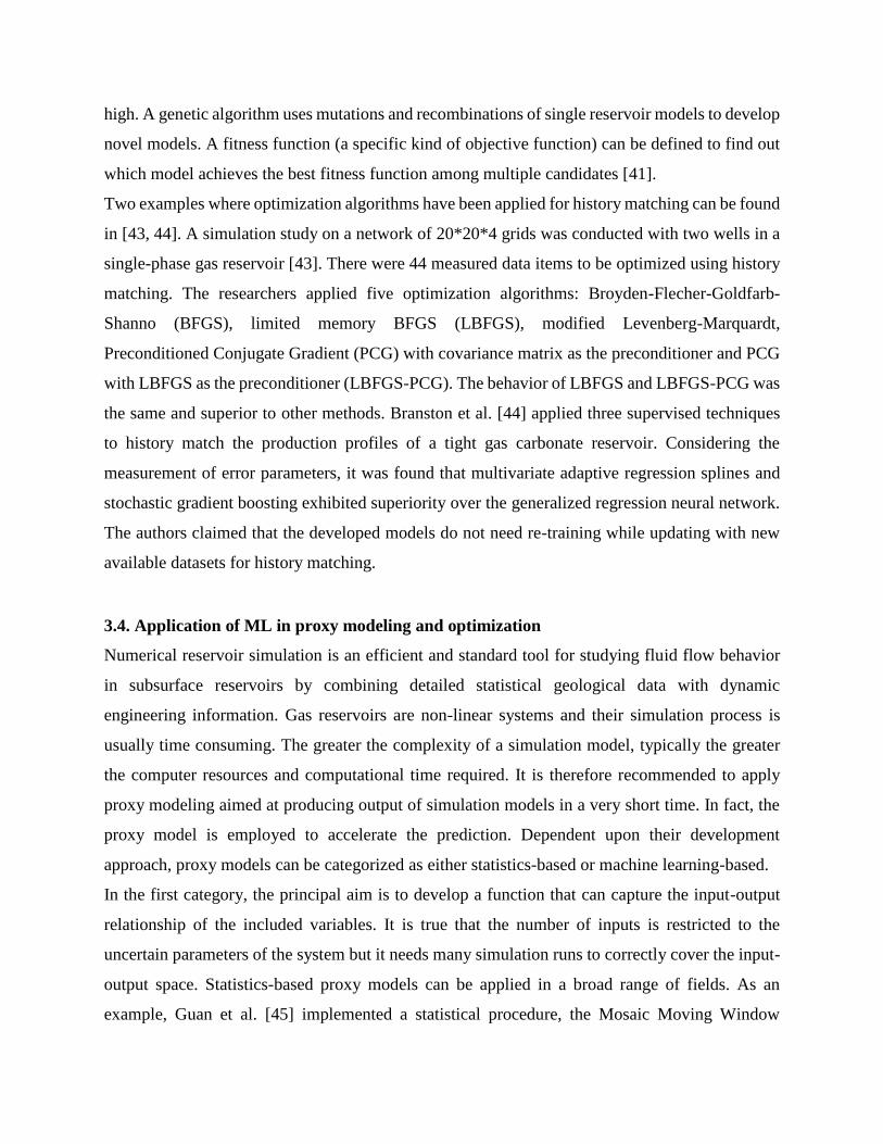
high. A genetic algorithm uses mutations and recombinations of single reservoir models to develop

novel models. A fitness function (a specific kind of objective function) can be defined to find out

which model achieves the best fitness function among multiple candidates [41].

Two examples where optimization algorithms have been applied for history matching can be found

in [43, 44]. A simulation study on a network of 20*20*4 grids was conducted with two wells in a

single-phase gas reservoir [43]. There were 44 measured data items to be optimized using history

matching. The researchers applied five optimization algorithms: Broyden-Flecher-Goldfarb-

Shanno (BFGS), limited memory BFGS (LBFGS), modified Levenberg-Marquardt,

Preconditioned Conjugate Gradient (PCG) with covariance matrix as the preconditioner and PCG

with LBFGS as the preconditioner (LBFGS-PCG). The behavior of LBFGS and LBFGS-PCG was

the same and superior to other methods. Branston et al. [44] applied three supervised techniques

to history match the production profiles of a tight gas carbonate reservoir. Considering the

measurement of error parameters, it was found that multivariate adaptive regression splines and

stochastic gradient boosting exhibited superiority over the generalized regression neural network.

The authors claimed that the developed models do not need re-training while updating with new

available datasets for history matching.

3.4. Application of ML in proxy modeling and optimization

Numerical reservoir simulation is an efficient and standard tool for studying fluid flow behavior

in subsurface reservoirs by combining detailed statistical geological data with dynamic

engineering information. Gas reservoirs are non-linear systems and their simulation process is

usually time consuming. The greater the complexity of a simulation model, typically the greater

the computer resources and computational time required. It is therefore recommended to apply

proxy modeling aimed at producing output of simulation models in a very short time. In fact, the

proxy model is employed to accelerate the prediction. Dependent upon their development

approach, proxy models can be categorized as either statistics-based or machine learning-based.

In the first category, the principal aim is to develop a function that can capture the input-output

relationship of the included variables. It is true that the number of inputs is restricted to the

uncertain parameters of the system but it needs many simulation runs to correctly cover the input-

output space. Statistics-based proxy models can be applied in a broad range of fields. As an

example, Guan et al. [45] implemented a statistical procedure, the Mosaic Moving Window

Method (MMWM), to appraise infill production potential in mature, tight gas formations. This

method did not require significant amounts of data and was also efficient. The results achieved by

MMWM and the subsequent simulation demonstrated the high accuracy of MMWM , but only for

a group of infill candidates, meaning that it was not appropriate for individual wells.

Machine learning-based proxy models are directed at understanding the complex dependency

between input and output parameters in the numerical simulation. A proxy model with the aid of

machine learning was developed for a real case carbon dioxide sequestration to investigate the

effect of pressure, saturation and CO2 mole fraction under different conditions [46]. The

underlying case was a depleted gas reservoir located 6561 ft underground with a thickness of 110

ft. The proxy model was able to generate results more quickly than common simulators.

An important point is that each proxy model is constructed based upon a corresponding specific

reservoir. In other words, the proxy model is not comprehensive and can only be utilized with

respect to the corresponding reservoir. To overcome this issue, the Deep Net Simulator (DNS) was

developed as a more general tool to instantly predict the pressure of hydraulically fractured tight

gas reservoirs using 140 case studies and applying deep learning [47]. Compared to conventional

simulators, the DNS depends only on a few factors, such as the properties of the focused grid cell,

its distance to the wellbore, production settings and initial condition; meaning that this procedure

is independent of other cells.

In addition to the application of ML in proxy modeling, it can also be very helpful to reservoir

simulation in other ways when the governing equations are appropriately understood and the

simulated model tuned. For instance, ML can be applied in the context of enhanced gas recovery,

well placement optimization, production optimization, estimation of gas production and pressure

and rate transient analysis, and examples of such applications are provided in the following

paragraphs.

In addition to deep saline formations and depleted oil reservoirs, depleted natural gas reservoirs

seem to be suitable locations for geologic carbon sequestration because of the integrity of their

reservoir seals and low risk of gas escape / leakage, provided there is enough information available

for their historic gas production and the necessary infrastructure (i.e., wells and flowlines) are in

place. Additionally, the average gas recovery factor for depleted gas fields is approximately 75%,

implying that enhanced gas recovery methods would be able to mobilize at least some of the 25%

or so of the gas remaining in a reservoir [46]. Carbon sequestration can hence be linked to enhanced

gas production by injecting CO2 into gas reservoirs and thereby enhancing natural gas recovery.

Zangeneh et al. [49] attempted to optimize the key parameters of enhanced gas recovery and carbon

dioxide storage using a genetic algorithm based on a selected sector of a real gas field in Asia. The

impact of CO2 solubility in the connate water was also analyzed. The results confirmed the

possibility of both the production of residual gas and the permanent storage of substantial amounts

of CO2. The dissolution of CO2 in reservoir connate water could also postpone/delay CO2

breakthrough in parts of the reservoir.

Determination of ideal horizontal well trajectories in the Frobisher gas field was performed using

the well length, azimuth, location and inclination inputs [50]. The optimization approach required

some manual analysis using a non-fully automatic technique. Schulze-Riegert et al. [51] addressed

the problem of horizontal well placement optimization considering the statistical geological

uncertainty for a case study on a North Sea gas condensate field. The authors parameterized the

search space based on the angular coordinates and selected the start and end point of the well

trajectory as design variables. A Monte Carlo-based sampling algorithm and a genetic algorithm

were used respectively for screening purposes and optimization.

A compositional reservoir simulation in order to optimize the production from gas condensate

reservoirs was presented by Udosen et al. [52]. To this end, three scenarios of water alternative

gas, cycling and pressure depletion were considered. After the simulation, it was understood that

the suggested methods could lead to considerable improvement in the recovery.

The goal of Al-Fattah & Startzman [53] was to develop a three-layer neural network-based model

to predict natural gas production in the USA from 1998 to 2020. They forecasted that the 1998 gas

supply would decrease at a rate of 1.8% per year in 1999 continued to the year 2001. Then, the

production would increase with an average rate of around 0.5% annually from 2002 to 2012. The

growth would be approximately 1.3% per year during the period of 2013 to 2020. We cannot

unfortunately assess the effectiveness and robustness of such a framework because of our limited

access to the real data. Jin [54] applied several machine learning methods to predict the expected

ultimate gas recovery of multiple shale gas wells. Jin analyzed 200 Barnett shale gas wells and

predicted the production profile of each well through the Arps hyperbolic decline model.

Comparisons of neural network, support vector machine and random forest models revealed that

neural network achieved the highest accuracy. Lee et al. [55] developed a deep learning-based

algorithm to estimate shale gas production using just two input parameters (i.e., production volume

and the shut-in period) from 315 wells located in Canada. The results indicated that the two-feature

case had a better performance in comparison with the case that only considered gas production

volumes as input. Ipeka et al. [56] applied two machine learning methods, an ANN and a

generalized linear model to predict the initial gas production rate of tight gas formations. The

former resulted in a mean squared error of 1.24, while the latter achieved a mean squared error of

1.57.

The principal goal of Gaw [57] was to construct an ANN with the capability of pressure and rate

transient analyses for dry, wet, and condensate gas reservoirs with a fixed composition. Production

profiles, well parameters and reservoir characteristics were input to the networks and each variable

was then predicted by the other two. There was a good match between the output of networks and

the real data.

4. Case study: dew point prediction for gas condensate reservoirs

This case applies ML to the simulation of natural gas reservoirs operation, focusing on dew point

pressure (Pd) prediction. Two ML models are described and their performances compared.

4.1. Dew point pressure

Dew point pressure (Pd) is a significant parameter for characterizing gas condensate reservoirs. It

is defined as the pressure at which the first liquid condenses from the gas at a fixed temperature.

The proper calculation of this property is essential to meet the optimal development and

management of these reservoirs. The experimental determination of Pd is typically conducted by

the constant volume depletion and/or constant composition expansion tests [58, 59]. Such tests are

authentic, but time-consuming and costly. The empirical equations [60], and graphical and matrix

methods for estimating Pd [61] cover limited operational conditions and are useful for only a few

specific cases. Equations of state require tuning against experimental data, which is usually done

in a trial and error manner. In this context, the incorrect characterization of the heptane plus (C7+)

fraction and the convergence problem may be encountered [62]. The case study presented here

considers two models to predict Pd over a wide range of conditions. The first model is an Artificial

Neural Network (ANN) which is trained using the Teaching-Learning-Based Optimization

(TLBO) algorithm. The second is constructed with a Convolutional Neural Network (CNN), a

class of deep neural networks. The performance of both models is evaluated using graphical and

statistical analyses.

4.2. Data analysis

The input parameters for a neural network should be selected carefully and with high sensitivity

so as to construct a trustworthy model. It is generally accepted [58, 59] that the mole fraction of

hydrocarbon and non-hydrocarbon components, characteristics of C7+, as well as temperature

influence the dew point pressure. For this case study, 632 data records over a wide temperature

range of [40 – 320 ˚F] were compiled from the literature [58, 59]. Table 1 presents details of the

dependent and independent variables considered.

Table 1 Statistical summary of the data variables associated with 632 data records from

several gas condensate fields evaluated in the case study.

Parameter Type Unit Minimum Average Maximum

Pd Output Psia 1405 4668.23 10500

T Input Fahrenheit 40 204.34 320

C1 Input Mole fraction 0.0349 0.8009 0.967




C5 Input Mole fraction 0 0.012 0.123

C6 Input Mole fraction 0 0.009 0.111

C7+ Input Mole fraction 0 0.035 0.136

N2 Input Mole fraction 0 0.013 0.432

CO2 Input Mole fraction 0 0.0155 0.919

H2S Input Mole fraction 0 0.006 0.3

SGC7+ Input Unitless 0 0.775 1

MWC7+ Input Gr/mol 0 144.48 235

4.3. ANN-TLBO model design

Seven basic steps were employed in the development of the ANN-TLBO model coded using

MatLab software. Step 1 involves data loading in the form of an ‘xlsx’ Microsoft Excel file. Step

2 normalizes the loaded data with each variable scaled into the range of [0 – 1]. Step 3 divides the

data into three subsets: (i) training (70%), (ii) validation (5%) and (iii) testing (25%). The model

learns based on the information contained in the training subset. The validation subset is utilized

to appraise the model during training process; it indirectly influences the given model. The testing

subset data is only used to evaluate the model’s accuracy once the model has been trained. Step 4

constructed a four-layer neural network comprising of (i) an input layer with 13 neurons

(independent variables), (ii) two hidden layers with 8 and 6 neurons respectively and (iii) an output

layer with one neuron (representing the dependent variable Pd). The activation functions applied

to the input to first hidden layer, first to second hidden layers, and second hidden layer to output

layer were respectively ‘tansig’, ‘logsig’, and ‘purelin’. Step 5 was the training phase conducted

using the TLBO algorithm [63]; comprising two main elements, teacher and learners, which

together train the ANN. TLBO, like other evolutionary algorithms, is initialized by a set of random

solutions; for this case study 400 solutions and maximum iteration of 1000 were selected.

However, TLBO has no tuning parameters, unlike other network training algorithms. Steps 6 and

7 evaluate the model’s performance by calculating various prediction accuracy parameters and

data visualization.

4.4. CNN model design

The CNN model [64] used is available with the Anaconda Distribution of the Python programing

language. Although CNN was designed for problems with two-dimensional arrays such as image

data, it is also applicable for one-dimensional regression-type problems. Before coding, the

‘numpy’, ‘pandas’, ‘sklearn’ and ‘keras (using tensorflow backend)’ libraries were loaded into the

‘Spyder’ module of Anaconda. The first three steps of the ANN-TLBO model were repeated after

loading the required libraries. Note that the input data has two dimensions consisting of the number

of samples (i.e., 632) and the number of features (i.e., 13). A third dimension was added to

represent the number of the single input row, resulting in an input data array in the form [632, 13,

1]. Step 4 defines a sequential model by adding (i) a one-dimensional convolutional layer

(‘Conv1D’), (ii) a ‘Flatten’ layer and (iii) three ‘Dense’ layers with 10, 14 and 1 neurons,

respectively. The single neuron in the dense layer represents the estimate of the dependent variable

Pd. Then, the model was compiled with mean squared error as the loss (objective) function, and

‘Adam’ [65] as the optimizer. The intuition behind the Adam optimization algorithm comes from

the concept of adaptive moment estimation. It is a combination of Root Mean Square Propagation

(RMSProp) and Stochastic Gradient Descent (SGD) with momentum. Like RMSProp, Adam

utilizes the squared gradients to scale the learning rate. Rather than using gradient alone, it

simultaneously makes use of the momentum via the moving average of the gradient, in a similar

way to SGD but with the additional aid of momentum. Step 5 trains the model with the training

subset evaluating 1000 epochs. Steps 6 and 7 evaluate prediction accuracy and visualize the results.

The latter was achieved using the Microsoft Excel.

4.5 Overfitting and Appropriate Remedies

The statistical term of ‘goodness of fit’ refers to how well a model’s predicted values fit the

measured (actual) ones. A predictive model that performs unfavorably on a training data set is

considered to ‘under-fit’ that data, because it is not able to establish a sufficiently accurate

relationship between predicted and actual values. On the other hand, a model that fits the noise in

present in the training data records, typically does not generalize very well when applied to other

data points (e.g. an independent validation or testing subset), because it has over-fitted the training

subset data records. Inspection of the prediction errors obtained for the different subsets evaluated

in this case study (Table 2) indicate that neither under-fitting (under-training) nor over-fitting

(over-training) is an issue for the ANN-TLBO and CNN models applied to the dataset considered..

However, if over-fitting occurs with other data sets, there are some techniques that can be applied

to reduce its impacts. The performance of a model can be, in some cases, influenced by the number

of data records being too few, especially when applying deep learning algorithms. Hence,

expanding the number of data records evaluated, if possible, is a solution to improve a model’s

accuracy in such cases. Another strategy to mitigate over-fitting is to initiate early stopping criteria

during the execution of the algorithm. The training process proceeds iteratively, and it is possible

to measure how well a model performs on different data subsets in each iteration. The accuracy

that can be achieved by a model on independent testing data records (i.e. those data records not

considered as part of the training subset) might be limited beyond a certain point. Early stopping

rules can provide guidance as to the maximum number of iterations that should be run, thereby

preventing the algorithm from over-fitting the training dataset. An over-fitted model usually takes

all input variables into account, while some have a limited effect on output(s). Determining and

removing less-important features (feature selection) is another way to prevent overfitting and

simplify models but is not always feasible. Alternatively regularization methods can be applied,

such as minimizing the complexity of a model by penalizing its loss (cost) function.

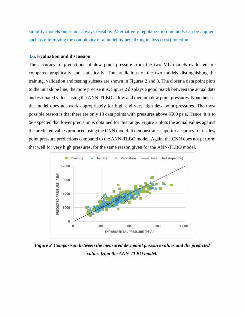
4.6. Evaluation and discussion

The accuracy of predictions of dew point pressure from the two ML models evaluated are

compared graphically and statistically. The predictions of the two models distinguishing the

training, validation and testing subsets are shown in Figures 2 and 3. The closer a data point plots

to the unit slope line, the more precise it is. Figure 2 displays a good match between the actual data

and estimated values using the ANN-TLBO at low and medium dew point pressures. Nonetheless,

the model does not work appropriately for high and very high dew point pressures. The most

possible reason is that there are only 13 data points with pressures above 8500 psia. Hence, it is to

be expected that lower precision is obtained for this range. Figure 3 plots the actual values against

the predicted values produced using the CNN model. It demonstrates superior accuracy for its dew

point pressure predictions compared to the ANN-TLBO model. Again, the CNN does not perform

that well for very high pressures, for the same reason given for the ANN-TLBO model.

Figure 2 Comparison between the measured dew point pressure values and the predicted

values from the ANN-TLBO model.

0

3000

6000

9000

12000

0 3 0 0 0 6 0 0 0 9 0 0 0 1 2 0 0 0

PR

EDIC

TED

PR

ESSU

RE

(PSI

A)

EXPERIMENTAL PRESSURE (PSIA)

Training Testing Validation Linear (Unit slope line)

Figure 3 Comparison between the measured dew point pressure values and the predicted

values from the CNN model.

In Figure 4, the cumulative frequency versus the absolute relative error (%) (Equation 19) for the

ANN-TLBO is depicted with respect to the training, validation and testing data subsets. The graph

indicates the same trend for all data subsets. More specifically, approximately 60% of the data

points achieve an absolute relative error of less than 10%. Roughly 30% have an error between

10% and 20%. Only 2 data records of the training subset have an error higher than 70%. This is

also the case for the testing data set. A comparison of Figures 4 and 5 highlights the superior

performance, in terms of frequency distribution, of the CNN model compared to the ANN-TLBO.

More than 85% of the validation data has an absolute relative error of less than 10%. In the case

of the training set, only two points have an error above 30%. This analysis also indicates that the

CNN model accurately predicts all of the testing subset data records, except for five records.

𝑎𝑏𝑠𝑜𝑙𝑢𝑡𝑒 𝑟𝑒𝑙𝑎𝑡𝑖𝑣𝑒 𝑒𝑟𝑟𝑜𝑟 (%) = 100 ∗ 𝑎𝑏𝑠((𝑝𝑑,𝑖/𝑃 − 𝑝𝑑,𝑖/𝑀)/𝑝𝑑,𝑖/𝑀) (19)

where ‘abs’ refers to the absolute value.

0

3000

6000

9000

12000

0 3 0 0 0 6 0 0 0 9 0 0 0 1 2 0 0 0

PR

EDIC

TED

PR

ESSU

RE

(PSI

A)

EXPERIMENTAL PRESSURE (PSIA)

Training Testing Validation Linear (Unit slope line)

Figure 4 Cumulative frequency versus absolute relative error (%) for the ANN-TLBO model.

Figure 5 Cumulative frequency versus absolute relative error (%) for the CNN model.

Analysis of a range of extensively used prediction error accuracy parameters provides further

insight into the performance of two models. The error statistics considered are:

𝐴𝑣𝑒𝑟𝑎𝑔𝑒 𝑅𝑒𝑙𝑎𝑡𝑖𝑣𝑒 𝐸𝑟𝑟𝑜𝑟 (𝐴𝑅𝐸 %) =

100 × ∑(𝑝𝑑,𝑖/𝑃 − 𝑝𝑑,𝑖/𝑀)

𝑝𝑑,𝑖/𝑀

𝑁𝑖=1

𝑁

(20)

0

0.1

0.2

0.3

0.4

0.5

0.6

0.7

0.8

0.9

1

0 1 0 2 0 3 0 4 0 5 0 6 0 7 0 8 0 9 0 1 0 0 1 1 0 1 2 0

CU

MU

LATI

VE

FREQ

UEN

CY

ABSOLUTE RELATIVE ERROR (%)

Training Validation Testing

0

0.1

0.2

0.3

0.4

0.5

0.6

0.7

0.8

0.9

1

0 1 0 2 0 3 0 4 0 5 0 6 0 7 0

CU

MU

LATI

VE

FREQ

UEN

CY

ABSOLUTE RELATIVE ERROR (%)

Training Validation Testing

𝑅𝑜𝑜𝑡 𝑀𝑒𝑎𝑛 𝑆𝑞𝑢𝑎𝑟𝑒 𝐸𝑟𝑟𝑜𝑟 (𝑅𝑀𝑆𝐸) = √∑ [(𝑝𝑑,𝑖/𝑃 − 𝑝𝑑,𝑖/𝑀)]2𝑛

𝑖=1

𝑁

(21)

𝑐𝑜𝑒𝑓𝑓𝑖𝑐𝑖𝑒𝑛𝑡 𝑜𝑓 𝑑𝑒𝑡𝑒𝑟𝑚𝑖𝑛𝑎𝑡𝑖𝑜𝑛 (𝑅2) = 1 −∑ (𝑝𝑑,𝑖/𝑃 − 𝑝𝑑,𝑖/𝑀)2𝑁

𝑖=1

∑ (𝑝𝑑,𝑖/𝑃 − 𝑝𝑑,𝑎𝑣𝑔/𝑀)2𝑁𝑖=1

(22)

𝑝𝑑,𝑖/𝑀, 𝑝𝑑,𝑖/𝑃 and 𝑝𝑑,𝑎𝑣𝑒/𝑀 are measured 𝑝𝑑, predicted 𝑝𝑑 and average of measured 𝑝𝑑,

respectively. In all cases, 𝑝𝑑 is expressed in psia. These three error parameters calculated for the

training, validation, and testing data subsets and the total dataset are listed in Table 2. According

to the last column, there is a slight improvement in R2 when the CNN model is applied to the entire

data set, and considerable improvement with respect to the RMSE value as it decreases from 646

to 455. However, Table 1 reveals the superior performance of the ANN-TLBO model, compared

to the CNN, in terms of the ARE error parameter. Considering all the error parameters calculated,

it is concluded that the accuracy of both models is satisfactory for all data subsets evaluated with

the CNN model outperforming the ANN-TLBO overall.

Table 2 Performance of the developed models based upon three statistical error metrics.

Error statistic Model Training set Validation set Testing set Total

ARE(%) ANN-TLBO 1.86 -0.69 2.72 1.948

CNN 4.29 1.72 5.09 4.36

RMSE ANN-TLBO 643.5 803.7 616 646

CNN 424 490 528 455

R2 ANN-TLBO 0.983 0.971 0.983 0.982

CNN 0.993 0.99 0.989 0.992

In summary, comparison between the two models using the measured Pd values and their

corresponding estimated values showed that, although both models could yield satisfactory results,

the CNN model had better performance overall with an ARE of 4.36, RMSE of 455 and R2 of

0.992. Ensuring there are sufficient numbers of data records across the entire Pd data range of

interest is essential for establishing a model with R2 of very close to 1. The addition of data points

to the dataset with Pd > 8500 psi could further improve the accuracy achieved by these two models.

Retrograde gas condensate reservoirs are thermodynamically more complex than other types of

subsurface gas reservoir. When the bottom-hole pressure falls below the dew point pressure (Pd),

condensate begins to condense in the reservoir zone surrounding the well bore. That condensed

liquid does not flow and remains trapped in the reservoir as long as its saturation remains the

critical saturation level. In order to design effective production schemes for gas condensate

reservoirs production and accurately simulate the behavior of such reservoirs as pressure changes,

accurate determination of Pd using the two models of ANN-TLBO and CNN should be beneficial.

Accurate Pd measurements help to maximize gas production and condensate recovery in such

reservoirs.

5. Summary

This chapter describes how the tools and techniques of machine learning can be employed to

support and enhance natural gas reservoir simulations. The fundamental concepts and key

principles involved in reservoir simulation are well established and the basic governing equations

applicable for gas reservoir simulations are described. Applying machine learning methods to gas

reservoir simulations adds enhancements and advanced benefits. In this context, the benefits fall

into four distinct areas of application: (i) the preparation of the data required to realize reservoir

simulation, (ii) the tuning of the governing equations, (iii) the application of ML techniques to

history matching, and (iv) the support that ML can provide for proxy modeling. Additionally, ML

can assist reservoir simulation analysis in assessing CO2 sequestration and enhanced gas recovery,

well placement optimization, production optimization, estimation of gas production, dew point

prediction in gas condensate reservoirs and pressure and rate transient analysis. Achieving

improvements in many aspects of reservoir performance make ML-assisted reservoir simulation a

useful tool in ensuring the long-term sustainability of natural gas reservoirs. A case study directed

at dew point pressure prediction reinforces the benefits that ML can bring to reservoir simulation

analysis. Two learning models are compared in the case study, (i) an Artificial Neural Network

trained using Teaching-Learned-Based Optimization, ANN-TLBO model, and (ii) a Convolutional

Neural Network (CNN) model. The CNN model was found to provide more accurate and reliable

prediction performance.

Acknowledgements

This work is partially supported by the Key Program Special Fund at Xi'an Jiaotong-Liverpool

University (XJTLU) (KSF-E-50, KSF-P-02) and XJTLU Research Development Funding (RDF-

19-01-15).

Declaration

The authors confirm that they have no conflicts of interest in regards to the content of this study.

References

[1] Katz DL, Lee RL. Natural gas engineering: production and storage. McGraw-Hill Economics

Department; 1990.

[2] Schilthuis RJ. Active oil and reservoir energy. Transactions of the AIME. 1936;118(01):33-

52.

[3] Ertekin T, Abou-Kassem JH, King GR. Basic applied reservoir simulation. Richardson, TX:

Society of Petroleum Engineers; 2001.

[4] Chen Z. Reservoir simulation: mathematical techniques in oil recovery. Society for Industrial

and Applied Mathematics; 2007.

[5] Darcy HP. Les Fontaines publiques de la ville de Dijon. Exposition et application des principes

à suivre et des formules à employer dans les questions de distribution d'eau, etc. V. Dalamont;

1856.

[6] Bishop CM. Neural networks for pattern recognition. Oxford university press; 1995.

[7] Jang JS. ANFIS: adaptive-network-based fuzzy inference system. In: IEEE transactions on

systems, man, and cybernetics; 1993;23(3):665-85.

[8] Vapnik V. Statistical learning theory; 1998 New York, NY.

[9] Espinoza M, Suykens JA, De Moor B. Least squares support vector machines and primal space

estimation. In: 42nd IEEE International Conference on Decision and Control (IEEE Cat. No.

03CH37475); 2003;4:3451-56.

[10] Ghorbani H, Wood DA, Choubineh A, Tatar A, Abarghoyi PG, Madani M, Mohamadian N.

Prediction of oil flow rate through an orifice flow meter: Artificial intelligence alternatives

compared. Petroleum. 2018.

[11] Ghorbani H, Wood DA, Moghadasi J, Choubineh A, Abdizadeh P, Mohamadian N. Predicting

liquid flow-rate performance through wellhead chokes with genetic and solver optimizers: An oil

field case study. Journal of Petroleum Exploration and Production Technology. 2019;9(2):1355-

73.

[12] Razavi R, Sabaghmoghadam A, Bemani A, Baghban A, Chau KW, Salwana E. Application

of ANFIS and LSSVM strategies for estimating thermal conductivity enhancement of metal and

metal oxide based nanofluids. Engineering Applications of Computational Fluid Mechanics.

2019;13(1):560-78.

[13] Menad NA, Noureddine Z, Hemmati-Sarapardeh A, Shamshirband S. Modeling temperature-

based oil-water relative permeability by integrating advanced intelligent models with grey wolf

optimization: application to thermal enhanced oil recovery processes. Fuel. 2019;242:649-63.

[14] Sousa AL, Ribeiro TP, Relvas S, Barbosa-Póvoa A. Using machine learning for enhancing

the understanding of bullwhip effect in the oil and gas industry. Machine Learning and Knowledge

Extraction. 2019;1(3):994-1012.

[15] Choubineh A, Wood DA, Choubineh Z. Applying separately cost-sensitive learning and

Fisher's discriminant analysis to address the class imbalance problem: A case study involving a

virtual gas pipeline SCADA system. International Journal of Critical Infrastructure Protection.

2020:100357.

[16] Hosseini AH, Ghadery-Fahliyany H, Wood DA, Choubineh A. Artificial intelligence-based

modeling of interfacial tension for carbon dioxide storage. Gas Processing Journal. 2020;8(1):83-

92.

[17] Rolon L, Mohaghegh SD, Ameri S, Gaskari R, McDaniel B. Using artificial neural networks

to generate synthetic well logs. Journal of Natural Gas Science and Engineering. 2009;1(4-5):118-

33.

[18] Elphick RY, Moore WR. Permeability calculations from clustered electrofacies, a case study

in Lake Maracaibo, Venezuela. InSPWLA 40th Annual Logging Symposium 1999. Society of

Petrophysicists and Well-Log Analysts.

[19] Xu C, Richter P, Russell D, Gournay J. Porosity partitioning and permeability quantification

in vuggy carbonates using wireline logs, Permian Basin, West Texas. Petrophysics. 2006;47(01).

[20] Zhou ZH. Ensemble Learning. Encyclopedia of biometrics. 2009:270-3.

[21] Anifowose FA, Labadin J, Abdulraheem A. Ensemble model of non-linear feature selection-

based extreme learning machine for improved natural gas reservoir characterization. Journal of

Natural Gas Science and Engineering. 2015;26:1561-72.

[22] Zendehboudi S, Ahmadi MA, James L, Chatzis I. Prediction of condensate-to-gas ratio for

retrograde gas condensate reservoirs using artificial neural network with particle swarm

optimization. Energy & Fuels. 2012;26(6):3432-47.

[23] Amiri M, Ghiasi-Freez J, Golkar B, Hatampour A. Improving water saturation estimation in

a tight shaly sandstone reservoir using artificial neural network optimized by imperialist

competitive algorithm–A case study. Journal of Petroleum Science and Engineering.

2015;127:347-58.

[24] Singh S, Kanli AI, Sevgen S. A general approach for porosity estimation using artificial neural

network method: a case study from Kansas gas field. Studia Geophysica et Geodaetica.

2016;60(1):130-40.

[25] Zhong Z, Liu S, Kazemi M, Carr TR. Dew point pressure prediction based on mixed-kernels-

function support vector machine in gas-condensate reservoir. Fuel. 2018;232:600-9.

[26] Xiong W, Ji X, Ma Y, Wang Y, AlBinHassan NM, Ali MN, Luo Y. Seismic fault detection

with convolutional neural network. Geophysics. 2018;83(5):O97-103.

[27] Zarifi A, Daryasafar A. Auto-tune of PVT data using an efficient engineering method:

Application of sensitivity and optimization analyses. Fluid Phase Equilibria. 2018;473:70-9.

[28] Forchheimer P. Wasserbewegung durch boden. Z. Ver. Deutsch, Ing. 1901;45(50):1782-8.

[29] Pascal H, Quillian RG. Analysis of vertical fracture length and non-Darcy flow coefficient

using variable rate tests. In: SPE Annual Technical Conference and Exhibition 1980. Society of

Petroleum Engineers.

[30] Li D, Svec RK, Engler TW, Grigg RB. Modeling and simulation of the wafer non-Darcy flow

experiments. In: SPE Western Regional Meeting 2001. Society of Petroleum Engineers.

[31] Thauvin F, Mohanty KK. Network modeling of non-Darcy flow through porous media.

Transport in Porous Media. 1998;31(1):19-37.

[32] Geertsma J. Estimating the coefficient of inertial resistance in fluid flow through porous

media. Society of Petroleum Engineers Journal. 1974;14(05):445-50.

[33] Kutasov IM. Equation predicts non-Darcy flow coefficient. Oil and Gas Journal;(United

States). 1993;91(11).

[34] Frederick Jr DC, Graves RM. New correlations to predict non-Darcy flow coefficients at

immobile and mobile water saturation. In: SPE Annual Technical Conference and Exhibition 1994.

Society of Petroleum Engineers.

[35] Efendiev Y, Galvis J, Hou TY. Generalized multiscale finite element methods (GMsFEM).

Journal of Computational Physics. 2013;251:116-35.

[36] Chen J, Chung ET, He Z, Sun S. Generalized multiscale approximation of mixed finite

elements with velocity elimination for subsurface flow. Journal of Computational Physics.

2020;404:109133.

[37] Evensen G, Hove J, Meisingset H, Reiso E, Seim KS, Espelid Ø. Using the EnKF for assisted

history matching of a North Sea reservoir model. In: SPE reservoir simulation symposium 2007.

Society of Petroleum Engineers.

[38] Anterion F, Eymard R, Karcher B. Use of parameter gradients for reservoir history matching.

In: SPE Symposium on Reservoir Simulation 1989. Society of Petroleum Engineers.

[39] Hu LY. Gradual deformation and iterative calibration of Gaussian-related stochastic models.

Mathematical Geology. 2000;32(1):87-108.

[40] Sambridge M. Geophysical inversion with a neighbourhood algorithm—II. Appraising the

ensemble. Geophysical Journal International. 1999;138(3):727-46.

[41] Schulze-Riegert RW, Axmann JK, Haase O, Rian DT, You YL. Evolutionary algorithms

applied to history matching of complex reservoirs. SPE Reservoir Evaluation & Engineering.

2002;5(02):163-73.

[42] Bouzarkouna Z, Nobakht B. A Better Formulation of Objective Functions for History

Matching Using Hausdorff Distances. In:EUROPEC. 2015. Society of Petroleum Engineers.

[43] Zhang F, Reynolds AC. E48: Optimization algorithms for automatic history matching of

production data. In:Proc. 8th Eur. Conf. Math. Oil Recovery 2002 (pp. 1-11).

[44] Brantson ET, Ju B, Omisore BO, Wu D, Selase AE, Liu N. Development of machine learning

predictive models for history matching tight gas carbonate reservoir production profiles. Journal

of Geophysics and Engineering. 2018;15(5):2235-51.

[45] Guan L, McVay DA, Jensen JL, Voneiff GW. Evaluation of a statistical method for assessing

infill production potential in mature, low-permeability gas reservoirs. J. Energy Resour. Technol..

2004;126(3):241-5.

[46] Amini S, Mohaghegh S. Application of machine learning and artificial intelligence in proxy

modeling for fluid flow in porous media. Fluids. 2019;4(3):126.

[47] Ghassemzadeh S, Perdomo MG, Abbasnejad E, Haghighi M. Modelling hydraulically

fractured tight gas reservoirs with an Artificial Intelligence (AI)-based simulator, Deep Net

Simulator (DNS). In: First EAGE Digitalization Conference and Exhibition 2020 (Vol. 2020, No.

1, pp. 1-5). European Association of Geoscientists & Engineers.

[48] Laherrère J. Distribution and evolution of “recovery factor,”. In: Oil Reserves Conference,

Paris, France 1997.

[49] Zangeneh H, Jamshidi S, Soltanieh M. Coupled optimization of enhanced gas recovery and

carbon dioxide sequestration in natural gas reservoirs: Case study in a real gas field in the south of

Iran. International Journal of Greenhouse Gas Control. 2013;17:515-22.

[50] Seifert D, Lewis JJ, Hern CY, Steel NC. Well placement optimisation and risking using 3-D

stochastic reservoir modelling techniques. In: European 3-D Reservoir Modelling Conference

1996. Society of Petroleum Engineers.

[51] Schulze-Riegert R, Ma D, Heskestad KL, Krosche M, Mustafa H, Stekolschikov K, Bagheri

M. Well path design optimization under geological uncertainty: Application to a complex North

Sea field. In: SPE Russian Oil and Gas Conference and Exhibition 2010. Society of Petroleum

Engineers.

[52] Udosen EO, Ahiaba OO, Aderemi SB. Optimization of gas condensate reservoir using

compositional reservoir simulator. In: Nigeria Annual International Conference and Exhibition

2010. Society of Petroleum Engineers.

[53] Al-Fattah SM, Startzman RA. Predicting natural gas production using artificial neural

network. In: SPE hydrocarbon economics and evaluation symposium 2001. Society of Petroleum

Engineers.

[54] Jin L. Machine learning aided production data analysis for estimated ultimate recovery

forecasting (Doctoral dissertation); 2018.

[55] Lee K, Lim J, Yoon D, Jung H. Prediction of shale-gas production at Duvernay Formation

using deep-learning algorithm. SPE Journal. 2019.

[56] Ikpeka PM, Amaechi UC, Xianlin M, Ugwu JO. Application of machine learning models in

predicting initial gas production rate from tight gas reservoirs. Rudarsko-geološko-naftni zbornik.

2019;34(3).

[57] Gaw H. Development of an artificial neural network for pressure and rate transient analysis

of horizontal wells completed in dry, wet and condensate gas reservoirs of naturally fractured

formations; 2014.

[58] Nemeth LK. A correlation of dew-point pressure with reservoir fluid composition and

temperature (Doctoral dissertation, Texas A&M University. Libraries); 1966.

[59] Nowroozi S, Ranjbar M, Hashemipour H, Schaffie M. Development of a neural fuzzy system

for advanced prediction of dew point pressure in gas condensate reservoirs. Fuel Processing

Technology. 2009;90(3):452-7.

[60] Elsharkawy AM. Predicting the dew point pressure for gas condensate reservoirs: empirical

models and equations of state. Fluid phase equilibria. 2002;193(1-2):147-65.

[61] Potsch KT, Braeuer L. A novel graphical method for determining dewpoint pressures of gas

condensates. In: European Petroleum Conference 1996. Society of Petroleum Engineers.

[62] Danesh A. PVT and phase behaviour of petroleum reservoir fluids. Elsevier; 1998.

[63] Rao RV, Savsani VJ, Vakharia DP. Teaching–learning-based optimization: an optimization

method for continuous non-linear large scale problems. Information sciences. 2012;183(1):1-5.

[64] LeCun Y, Haffner P, Bottou L, Bengio Y. Object recognition with gradient-based learning.

In: Shape, contour and grouping in computer vision 1999 (pp. 319-345). Springer, Berlin,

Heidelberg.

[65] Kingma DP, Ba J. Adam: A method for stochastic optimization. arXiv preprint

arXiv:1412.6980. 2014.

machine learning to improve natural gas reservoir simulations

Documents